Embed Size (px)
Citation preview

Training & testing
Based upon Chapter 5 of Data Mining

2Data Mining: Practical Machine Learning Tools and Techniques (Chapter 5)
Credibility: Evaluating what’s been learned
● Issues: training, testing, tuning● Predicting performance: confidence limits● Holdout, crossvalidation, bootstrap● Comparing schemes: the ttest● Predicting probabilities: loss functions● Costsensitive measures● Evaluating numeric prediction● The Minimum Description Length principle

3Data Mining: Practical Machine Learning Tools and Techniques (Chapter 5)
Evaluation: the key to success
● How predictive is the model we learned?● Error on the training data is not a good
indicator of performance on future data♦ Otherwise 1NN would be the optimum classifier!
● Simple solution that can be used if lots of (labeled) data is available:
♦ Split data into training and test set● However: (labeled) data is usually limited
♦ More sophisticated techniques need to be used

4Data Mining: Practical Machine Learning Tools and Techniques (Chapter 5)
Issues in evaluation
● Statistical reliability of estimated differences in performance (→ significance tests)
● Choice of performance measure:♦ Number of correct classifications♦ Accuracy of probability estimates ♦ Error in numeric predictions
● Costs assigned to different types of errors♦ Many practical applications involve costs

5Data Mining: Practical Machine Learning Tools and Techniques (Chapter 5)
Training and testing I
● Natural performance measure for classification problems: error rate
♦ Success: instance’s class is predicted correctly♦ Error: instance’s class is predicted incorrectly♦ Error rate: proportion of errors made over the
whole set of instances● Resubstitution error: error rate obtained
from training data● Resubstitution error is (hopelessly)
optimistic!

6Data Mining: Practical Machine Learning Tools and Techniques (Chapter 5)
Training and testing II
● Test set: independent instances that have played no part in formation of classifier● Assumption: both training data and test data are
representative samples of the underlying problem● Test and training data may differ in nature
● Example: classifiers built using customer data from two different towns A and B● To estimate performance of classifier from town A in completely
new town, test it on data from B

7Data Mining: Practical Machine Learning Tools and Techniques (Chapter 5)
Note on parameter tuning
● It is important that the test data is not used in any way to create the classifier
● Some learning schemes operate in two stages:● Stage 1: build the basic structure● Stage 2: optimize parameter settings
● The test data can’t be used for parameter tuning!● Proper procedure uses three sets: training data,
validation data, and test data● Validation data is used to optimize parameters

8Data Mining: Practical Machine Learning Tools and Techniques (Chapter 5)
Making the most of the data
● Once evaluation is complete, all the data can be used to build the final classifier
● Generally, the larger the training data the better the classifier (but returns diminish)
● The larger the test data the more accurate the error estimate
● Holdout procedure: method of splitting original data into training and test set● Dilemma: ideally both training set and test set should be
large!
9Data Mining: Practical Machine Learning Tools and Techniques (Chapter 5)
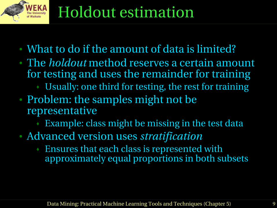
Holdout estimation
● What to do if the amount of data is limited?● The holdout method reserves a certain amount
for testing and uses the remainder for training♦ Usually: one third for testing, the rest for training
● Problem: the samples might not be representative
♦ Example: class might be missing in the test data● Advanced version uses stratification
♦ Ensures that each class is represented with approximately equal proportions in both subsets

10Data Mining: Practical Machine Learning Tools and Techniques (Chapter 5)
Repeated holdout method
● Holdout estimate can be made more reliable by repeating the process with different subsamples
♦ In each iteration, a certain proportion is randomly selected for training (possibly with stratificiation)
♦ The error rates on the different iterations are averaged to yield an overall error rate
● This is called the repeated holdout method● Still not optimum: the different test sets overlap
♦ Can we prevent overlapping?

11Data Mining: Practical Machine Learning Tools and Techniques (Chapter 5)
Crossvalidation
● Crossvalidation avoids overlapping test sets♦ First step: split data into k subsets of equal size♦ Second step: use each subset in turn for testing,
the remainder for training● Called kfold crossvalidation● Often the subsets are stratified before the
crossvalidation is performed● The error estimates are averaged to yield an
overall error estimate

12Data Mining: Practical Machine Learning Tools and Techniques (Chapter 5)
More on crossvalidation
● Standard method for evaluation: stratified tenfold crossvalidation
● Why ten?♦ Extensive experiments have shown that this is the best
choice to get an accurate estimate♦ There is also some theoretical evidence for this
● Stratification reduces the estimate’s variance● Even better: repeated stratified crossvalidation
♦ E.g. tenfold crossvalidation is repeated ten times and results are averaged (reduces the variance)

13Data Mining: Practical Machine Learning Tools and Techniques (Chapter 5)
LeaveOneOut crossvalidation
● LeaveOneOut:a particular form of crossvalidation:
♦ Set number of folds to number of training instances♦ I.e., for n training instances, build classifier n times
● Makes best use of the data● Involves no random subsampling ● Very computationally expensive
♦ (exception: NN)

14Data Mining: Practical Machine Learning Tools and Techniques (Chapter 5)
LeaveOneOutCV and stratification
● Disadvantage of LeaveOneOutCV: stratification is not possible
♦ It guarantees a nonstratified sample because there is only one instance in the test set!
● Extreme example: random dataset split equally into two classes
♦ Best inducer predicts majority class♦ 50% accuracy on fresh data ♦ LeaveOneOutCV estimate is 100% error!

15Data Mining: Practical Machine Learning Tools and Techniques (Chapter 5)
The bootstrap● CV uses sampling without replacement
● The same instance, once selected, can not be selected again for a particular training/test set
● The bootstrap uses sampling with replacement to form the training set● Sample a dataset of n instances n times with replacement
to form a new dataset of n instances● Use this data as the training set● Use the instances from the original
dataset that don’t occur in the newtraining set for testing

16Data Mining: Practical Machine Learning Tools and Techniques (Chapter 5)
The 0.632 bootstrap
● Also called the 0.632 bootstrap♦ A particular instance has a probability of 1–1/n
of not being picked♦ Thus its probability of ending up in the test
data is:
♦ This means the training data will contain approximately 63.2% of the instances
1− 1n n≈e−1≈0.368

17Data Mining: Practical Machine Learning Tools and Techniques (Chapter 5)
Estimating error with the bootstrap
● The error estimate on the test data will be very pessimistic
♦ Trained on just ~63% of the instances● Therefore, combine it with the
resubstitution error:
● The resubstitution error gets less weight than the error on the test data
● Repeat process several times with different replacement samples; average the results
err=0.632×etest instances0.368×etraining_instances

18Data Mining: Practical Machine Learning Tools and Techniques (Chapter 5)
More on the bootstrap
● Probably the best way of estimating performance for very small datasets
● However, it has some problems♦ Consider the random dataset from above♦ A perfect memorizer will achieve
0% resubstitution error and ~50% error on test data
♦ Bootstrap estimate for this classifier:
♦ True expected error: 50%
err=0.632×50%0.368×0%=31.6%

19Data Mining: Practical Machine Learning Tools and Techniques (Chapter 5)
Comparing data mining schemes
● Frequent question: which of two learning schemes performs better?
● Note: this is domain dependent!● Obvious way: compare 10fold CV estimates● Generally sufficient in applications (we don't
loose if the chosen method is not truly better)● However, what about machine learning research?
♦ Need to show convincingly that a particular method works better

20Data Mining: Practical Machine Learning Tools and Techniques (Chapter 5)
Comparing schemes II● Want to show that scheme A is better than scheme B in a
particular domain♦ For a given amount of training data♦ On average, across all possible training sets
● Let's assume we have an infinite amount of data from the domain:
♦ Sample infinitely many dataset of specified size♦ Obtain crossvalidation estimate on each dataset for
each scheme♦ Check if mean accuracy for scheme A is better than
mean accuracy for scheme B

21Data Mining: Practical Machine Learning Tools and Techniques (Chapter 5)
Paired ttest● In practice we have limited data and a limited
number of estimates for computing the mean● Student’s ttest tells whether the means of two
samples are significantly different● In our case the samples are crossvalidation
estimates for different datasets from the domain● Use a paired ttest because the individual samples
are paired♦ The same CV is applied twice
William GossetBorn: 1876 in Canterbury; Died: 1937 in Beaconsfield, EnglandObtained a post as a chemist in the Guinness brewery in Dublin in 1899. Invented the ttest to handle small samples for quality control in brewing. Wrote under the name "Student".

22Data Mining: Practical Machine Learning Tools and Techniques (Chapter 5)
Counting the cost
● The confusion matrix:
There are many other types of cost!● E.g.: cost of collecting training data
Actual class
True negativeFalse positiveNo
False negativeTrue positiveYes
NoYes
Predicted class

23Data Mining: Practical Machine Learning Tools and Techniques (Chapter 5)
Aside: the kappa statistic● Two confusion matrices for a 3class problem:
actual predictor (left) vs. random predictor (right)
● Number of successes: sum of entries in diagonal (D) ● Kappa statistic:
measures relative improvement over random predictor
Dobserved−Drandom
Dperfect−Drandom

24Data Mining: Practical Machine Learning Tools and Techniques (Chapter 5)
Classification with costs
● Two cost matrices:
● Success rate is replaced by average cost per prediction
♦ Cost is given by appropriate entry in the cost matrix

25Data Mining: Practical Machine Learning Tools and Techniques (Chapter 5)
Costsensitive classification
● Can take costs into account when making predictions♦ Basic idea: only predict highcost class when very
confident about prediction● Given: predicted class probabilities
♦ Normally we just predict the most likely class♦ Here, we should make the prediction that minimizes
the expected cost● Expected cost: dot product of vector of class probabilities
and appropriate column in cost matrix● Choose column (class) that minimizes expected cost

26Data Mining: Practical Machine Learning Tools and Techniques (Chapter 5)
Costsensitive learning
● So far we haven't taken costs into account at training time
● Most learning schemes do not perform costsensitive learning● They generate the same classifier no matter what
costs are assigned to the different classes● Example: standard decision tree learner
● Simple methods for costsensitive learning:● Resampling of instances according to costs● Weighting of instances according to costs
● Some schemes can take costs into account by varying a parameter, e.g. naïve Bayes

27Data Mining: Practical Machine Learning Tools and Techniques (Chapter 5)
Lift charts
● In practice, costs are rarely known● Decisions are usually made by comparing
possible scenarios● Example: promotional mailout to 1,000,000
households• Mail to all; 0.1% respond (1000)• Data mining tool identifies subset of 100,000
most promising, 0.4% of these respond (400)40% of responses for 10% of cost may pay off
• Identify subset of 400,000 most promising, 0.2% respond (800)
● A lift chart allows a visual comparison
28Data Mining: Practical Machine Learning Tools and Techniques (Chapter 5)
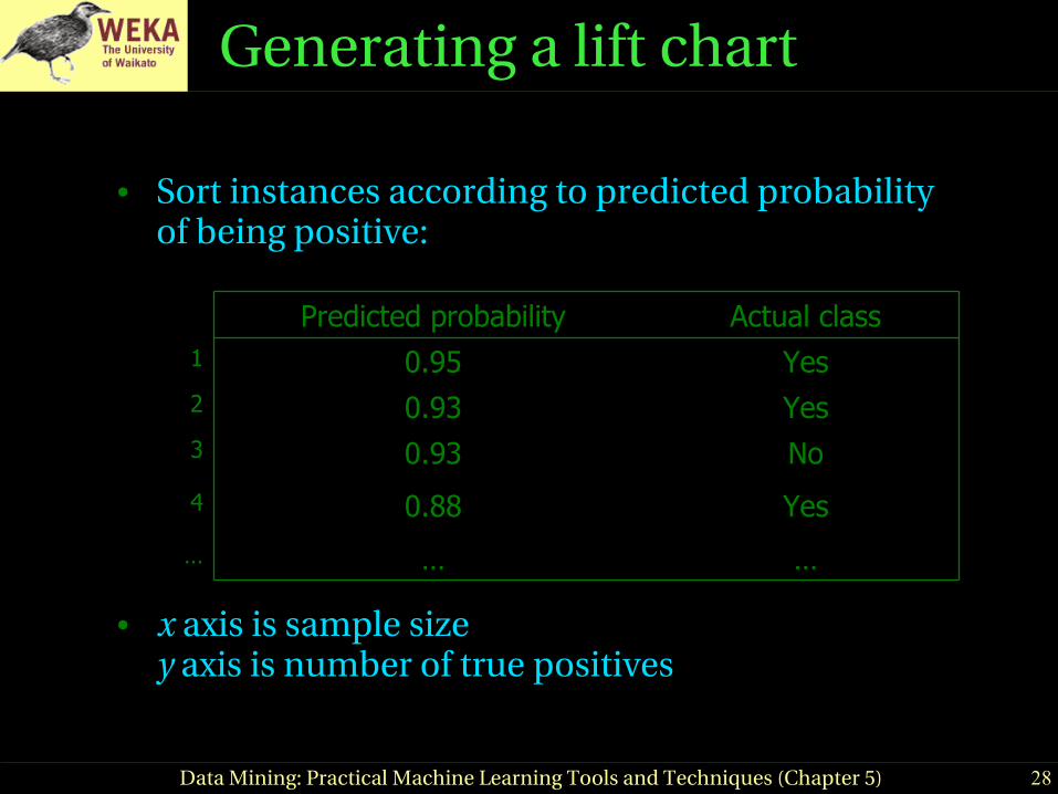
Generating a lift chart
● Sort instances according to predicted probability of being positive:
● x axis is sample sizey axis is number of true positives
………
Yes0.884
No0.933
Yes0.932
Yes0.951
Actual classPredicted probability

29Data Mining: Practical Machine Learning Tools and Techniques (Chapter 5)
A hypothetical lift chart
40% of responsesfor 10% of cost
80% of responsesfor 40% of cost

30Data Mining: Practical Machine Learning Tools and Techniques (Chapter 5)
ROC curves
● ROC curves are similar to lift charts♦ Stands for “receiver operating characteristic”♦ Used in signal detection to show tradeoff between
hit rate and false alarm rate over noisy channel● Differences to lift chart:
♦ y axis shows percentage of true positives in sample rather than absolute number
♦ x axis shows percentage of false positives in sample rather than sample size

31Data Mining: Practical Machine Learning Tools and Techniques (Chapter 5)
A sample ROC curve
● Jagged curve—one set of test data● Smooth curve—use crossvalidation

32Data Mining: Practical Machine Learning Tools and Techniques (Chapter 5)
Crossvalidation and ROC curves
● Simple method of getting a ROC curve using crossvalidation:
♦ Collect probabilities for instances in test folds♦ Sort instances according to probabilities
● This method is implemented in WEKA● However, this is just one possibility
♦ Another possibility is to generate an ROC curve for each fold and average them

33Data Mining: Practical Machine Learning Tools and Techniques (Chapter 5)
More measures...
● Percentage of retrieved documents that are relevant: precision=TP/(TP+FP)
● Percentage of relevant documents that are returned: recall =TP/(TP+FN)
● Precision/recall curves have hyperbolic shape● Summary measures: average precision at 20%, 50% and 80%
recall (threepoint average recall)● Fmeasure=(2 × recall × precision)/(recall+precision)● sensitivity × specificity = (TP / (TP + FN)) × (TN / (FP + TN))● Area under the ROC curve (AUC):
probability that randomly chosen positive instance is ranked above randomly chosen negative one

34Data Mining: Practical Machine Learning Tools and Techniques (Chapter 5)
Summary of some measures
ExplanationPlotDomain
TP/(TP+FN)TP/(TP+FP)
RecallPrecision
Information retrieval
Recall-precision curve
TP/(TP+FN)FP/(FP+TN)
TP rateFP rate
CommunicationsROC curve
TP(TP+FP)/(TP+FP+TN+FN)
TP Subset size
MarketingLift chart

35Data Mining: Practical Machine Learning Tools and Techniques (Chapter 5)
Evaluating numeric prediction
● Same strategies: independent test set, crossvalidation, significance tests, etc.
● Difference: error measures● Actual target values: a1 a2 …an
● Predicted target values: p1 p2 … pn
● Most popular measure: meansquared error
● Easy to manipulate mathematically
p1−a12...pn−an
2
n

36Data Mining: Practical Machine Learning Tools and Techniques (Chapter 5)
Other measures
● The root meansquared error :
● The mean absolute error is less sensitive to outliers than the meansquared error:
● Sometimes relative error values are more appropriate (e.g. 10% for an error of 50 when predicting 500)
p1−a12...pn−an
2
n
∣p1−a1∣...∣pn−an∣
n

37Data Mining: Practical Machine Learning Tools and Techniques (Chapter 5)
Improvement on the mean
● How much does the scheme improve on simply predicting the average?
● The relative squared error is:
● The relative absolute error is:
p1−a12...pn−an
2
a−a12...a−an
2
∣p1−a1∣...∣pn−an∣
∣a−a1∣...∣a−an∣

38Data Mining: Practical Machine Learning Tools and Techniques (Chapter 5)
Correlation coefficient
● Measures the statistical correlation between the predicted values and the actual values
● Scale independent, between –1 and +1● Good performance leads to large values!
SPA
SPSA
SP=∑i pi−p2
n−1 SA=∑i ai−a2
n−1SPA=
∑i pi−pai−a
n−1

39Data Mining: Practical Machine Learning Tools and Techniques (Chapter 5)
Which measure?
● Best to look at all of them● Often it doesn’t matter● Example:
0.910.890.880.88Correlation coefficient
30.4%34.8%40.1%43.1%Relative absolute error
35.8%39.4%57.2%42.2%Root rel squared error
29.233.438.541.3Mean absolute error
57.463.391.767.8Root mean-squared error
DCBA
● D best● C second-best● A, B arguable

40Data Mining: Practical Machine Learning Tools and Techniques (Chapter 5)
The MDL principle
● MDL stands for minimum description length● The description length is defined as:
space required to describe a theory + space required to describe the theory’s mistakes
● In our case the theory is the classifier and the mistakes are the errors on the training data
● Aim: we seek a classifier with minimal DL● MDL principle is a model selection criterion

41Data Mining: Practical Machine Learning Tools and Techniques (Chapter 5)
Model selection criteria
● Model selection criteria attempt to find a good compromise between:● The complexity of a model● Its prediction accuracy on the training data
● Reasoning: a good model is a simple model that achieves high accuracy on the given data
● Also known as Occam’s Razor :the best theory is the smallest onethat describes all the facts
William of Ockham, born in the village of Ockham in Surrey (England) about 1285, was the most influential philosopher of the 14th century and a controversial theologian.

42Data Mining: Practical Machine Learning Tools and Techniques (Chapter 5)
Elegance vs. errors
● Theory 1: very simple, elegant theory that explains the data almost perfectly
● Theory 2: significantly more complex theory that reproduces the data without mistakes
● Theory 1 is probably preferable● Classical example: Kepler’s three laws on
planetary motion♦ Less accurate than Copernicus’s latest refinement of
the Ptolemaic theory of epicycles

43Data Mining: Practical Machine Learning Tools and Techniques (Chapter 5)
MDL and compression
● MDL principle relates to data compression:● The best theory is the one that compresses the data
the most● I.e. to compress a dataset we generate a model and
then store the model and its mistakes● We need to compute
(a) size of the model, and(b) space needed to encode the errors
● (b) easy: use the informational loss function● (a) need a method to encode the model

44Data Mining: Practical Machine Learning Tools and Techniques (Chapter 5)
MDL and Bayes’s theorem
● L[T]=“length” of the theory● L[E|T]=training set encoded wrt the theory● Description length= L[T] + L[E|T]● Bayes’s theorem gives a posteriori probability of
a theory given the data:
● Equivalent to:
constant
Pr [T|E]=Pr [E|T]Pr [T ]
Pr [E]
−logPr[T|E]=−logPr[E|T]−logPr [T ]logPr [E]

45Data Mining: Practical Machine Learning Tools and Techniques (Chapter 5)
MDL and MAP
● MAP stands for maximum a posteriori probability● Finding the MAP theory corresponds to finding the
MDL theory● Difficult bit in applying the MAP principle:
determining the prior probability Pr[T] of the theory● Corresponds to difficult part in applying the MDL
principle: coding scheme for the theory● I.e. if we know a priori that a particular theory is
more likely we need fewer bits to encode it