8 TRANSPORTATION RESEARCH RECORD 1308

Train Operations Computer Simulation Case Study: Single-Tracking Operations for Philadelphia's Market-Frankford Subway Elevated Rail Rapid Transit Line

ERIC BRUUN AND p. TAKIS SALPEAS

The graphical portrayal of train operations using time-distance diagrams has long been used to develop schedules and for other analyses. The availability, however, of relatively simple , practi­cal, user-friendly computerized tools to do the related calculations and plots is limited. The development and application of a pack­age of PC-driv n programs that accurately simulnte train oper­ations, plots bidirectional operations charts and schedules, and allows sensitivity testing of various operating parameters are dis­cus ed . The package was te. Led using data derive from the op­erations of Philade lphia s Market -Frankford ubway elevated rail rapid tra nsit line. It thc11 successfully generated graphical sched­ule (string-chart) diagrams for this two-tra k line under a series of operating assumptions. f special inreres t was the IC. Ling of the pr ent chedulc while a ·cction of track 599 m (1,964 ft) long between two stations was taken out of service. Such a package can be easily developed and used for a variety of sensitivity anal­yses , graphical scheduling, and other operational tests .

Philadelphia's Market-Frankford subway elevated (MFSE) rail rapid transit line spans 21.24 km (13 .2 mi) and serves Center City through seven subway stations. This two-track line with 9 stations on the western elevated portion (Market El) and 12 stations on the eastern elevated portion (frankfurd El) carries nearly 200,000 passengers per day. Nearly one of every four Center City jobs is reached via this line. Its reliability and high-performance service are instrumental in the city's daily functioning. The Southeastern Pennsylvania Transpor­tation Authority (SEPTA) provides maximum service of up to 35 trains eastbound during the 2-hr p.m. peak period.

The eastern elevated portion is undergoing reconstruction. To minimize passenger disruption, SEPT A solicited compet­itive bids for the reconstruction of an elevated section on the basis of a one-track-at-a-time construction method. Bidirec­tional passenger service was to be continued on the basis of a single-tracking operations plan.

The PC-based simulation program described in this paper was an important tool in testing whether a single-tracking schedule could be developed to operate the number of trains that is normal when both tracks are in service. The formal scheduling for MFSE operations, however, was beyond the scope of this work . This schedule may be influenced by ad-

E. Bruun, University of Pennsylvania, 113 Towne Building, Phila­delphia, Pa. 19104. P. T. Salpeas, Southeastern Pennsylvania Trans­portation Authority , 5800 Bustleton Ave., Philadelphia, Pa. 19149.

ditional factors that can best be assessed by SEPT A's sched­uling and operations departments.

BACKGROUND

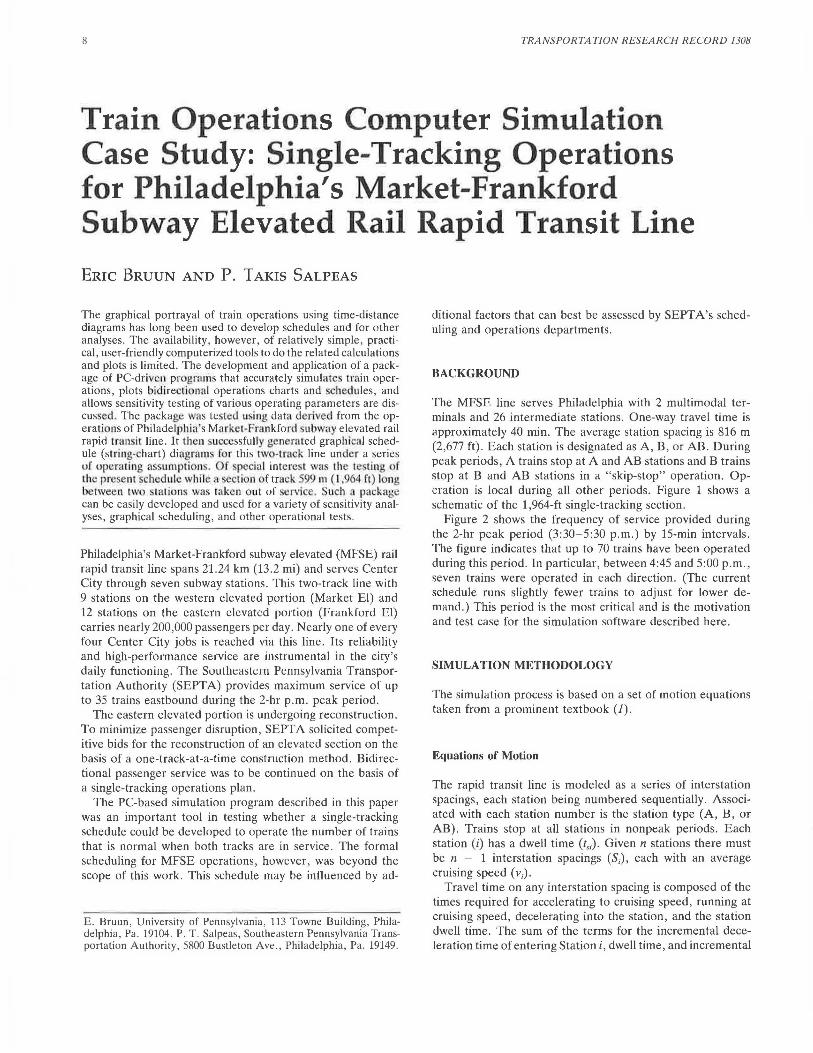
The MFSE line serves Philadelphia with 2 multimodal ter­minals and 26 intermediate stations. One-way travel time is approximately 40 min. The average station spacing is 816 m (2,677 ft). Each station is designated as A, B, or AB. During peak periods, A trains stop at A and AB stations and B trains stop at B and AB stations in a "skip-stop" operation. Op­eration is local during all other periods. Figure 1 shows a schematic of the 1,964-ft single-tracking section .

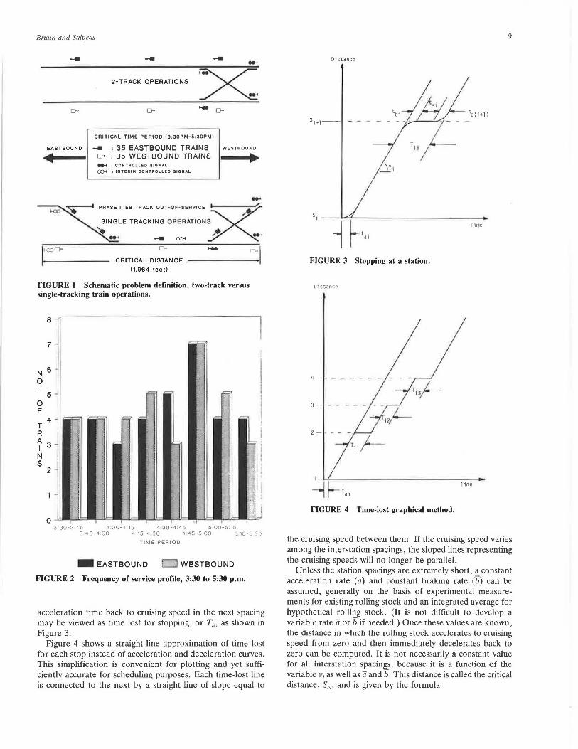
Figure 2 shows the frequency of service provided during the 2-hr peak period (3:30-5:30 p.m.) by 15-min intervals. The figure indicates that up to 70 trains have been operated during this period. In particular, between 4:45 and 5:00 p.m., seven trains were operated in each direction. (The current schedule runs slightly fewer trains to adjust for lower de­mand.) This period is the most critical Clnd is the motivation and test case for the simulation software described here .

SIMULATION METHODOLOGY

The simulation process is based on a set of motion equations taken from a prominent textbook (1).

Equations of Motion

The rapid transit line is modeled as a series of interstation spacings, each station being numbered sequentially. Associ­ated with each station number is the station type (A, H, or AB). Trains stop at all stations in nonpeak periods. Each station (i) has a dwell time (t,;) . Given n stations there must be n - 1 interstation spacings (S;), each with an average cruising speed (v;).

Travel time on any interstation spacing is composed of the times required for accelerating to cruising speed, running at cruising speed, decelerating into the station, and the station dwell time. The sum of the terms for the incremental dece­leration time of entering Station i , dwell time , and incremental

Bruun and Sa/peas

- -2-TRACK OPERATIONS x

[)o [)o ... [)o

CRITICAL TIME PERIOD (3 ,30PM-5,30PM)

EASTBOUND - : 35 EASTBOUND TRAINS WESTBOUND

~ o- : 35 WESTBOUND TRAINS .. ~ : CONTROLLED SIGNAL

a:H : INTERIM CONTROLLED SIGNAL

... ~ PHASE 1, EB TRACK OUT·OF•-SERVICE ~

SINGLE TRACKING OPERATIONS

:::.. ~ ... .... - co-<

[)o

CRITICAL DISTANCE

(1,964 feet)

0-1

FIGURE 1 Schematic problem definition, two-track versus single-tracking train operations.

8

7

N 6 0

0 F

T R

5

4

A 3 I N s

2

0 3 30-3:45 4:00-4:15 4 30-4:45 5:00-5:15

3:45 - 4 :00 4 15 - 4 30 4 45-5:00 5 15·o 2G

TIME PERIOD

-EASTBOUND LJ WESTBOUND

FIGURE 2 Frequency of service profile, 3:30 to 5:30 p.m.

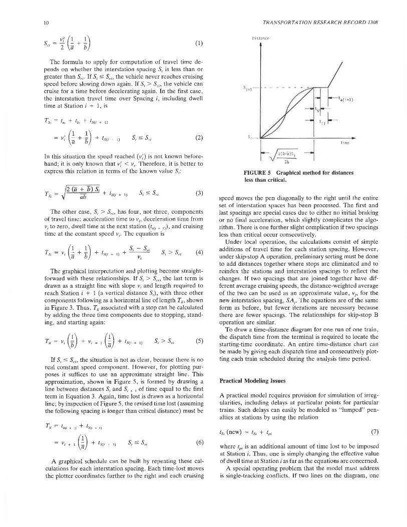
acceleration time back to cruising speed in the next spacing may be viewed as time lost for stopping, or T,,, as shown in Figure 3.

Figure 4 shows a straight-line approximation of time lost for each stop instead of acceleration and deceleration curves. This simplification is convenient for plotting and yet suffi­ciently accurate for scheduling purposes. Each time-lost line is connected to the next by a straight line of slope equal to

9

:Ji s ta nee

ta( i + 1) S; +1 - - - - - -

FIGURE 3 Stopping at a station.

Distance

FIGURE 4 Time-lost graphical method.

the cruising speed between them. If the cruising speed varies among the interstation spacings, the sloped lines representing the cruising speeds will no longer be parallel.

Unless the station spacings are extremely short, a constant acceleration rate (a) and constant braking rate (b) can be assumed, generally on the basis of experimental measure­ments for existing rolling stock and an integrated average for hypothetical rolling stock. (It is not difficult to develop a variable rate a orb if needed.) Once these values are known, the distance in which the rolling stock accelerates to cruising speed from zero and then immediately decelerates back to zero can be computed. It is not necessarily a constant value for all interstation spacings, because it is a function of the variable v, as well as a and b. This distance is called the critical distance, s ci > and is given by the formula

10

v2 (1 1)

sci= i ~ + 'b (1)

The formula to apply for computation of travel time de­pends on whether the interstation spacing S; is less than or greater than Sc;· If S; s Sc;, the vehicle never reaches cruising speed before slowing down again. If S1 > Sc1, the vehicle can cruise for a time before decelerating again. In the first case, the interstation travel time over Spacing i, including dwell time at Station i + 1, is

= v; ( ~ + ~) + lsu + 1) (2)

In this situation the speed reached (v;) is not known before­hand; it is only known that v; < v1• Therefore, it is better to express this relation in terms of the known value S1:

J2 (a+ b) s, Ts1 = ab + lsc1 + 1) (3)

The other case, S1 > Sc1, has four, not three, components of travel time: acceleration time to V;, deceleration time from V; to zero , dwell time at the next station (t,u + 1i) , and cruising time at the constant speed v1• The equation is

(1 1) S, - S" Ts, = V; ~ + b + fsc; + 1) + v, (4)

The graphical interpretation and plotting become straight­forward with these relationships. If S; > Sc;, the last term is drawn as a straight line with slope V; and length required to reach Station i + 1 (a vertical distance S;), with three other components following as a horizontal line of length Tli, shown in Figurt: 3. Thus, T1; assodatt:<l with a stop can be calculated by adding the three time components due to stopping, stand­ing, and starting again:

Tli = V; (~) + V; + 1 G) + lsu + 1) (5)

If S1 s Sci, the situation is not as clear , because there is no real constant speed component. However, for plotting pur­poses it suffices to use an approximate straight line. This approximation, shown in Figure 5, is formed by drawing a line between distances S1 and S; + 1 of time equal to the first term in Equation 3. Again, time lost is drawn as a horizontal line; by inspection of Figure 5, the revised time lost (assuming the following spacing is longer than critical distance) must be

V; + 1 G) + fsc; + 1) (6)

A graphical schedule can be built by repeating these cal­culations for each interstation spacing. Each time-lost moves the plotter coordinates further to the right and each cruising

TRANSPORTATION RESEARCH RECORD 1308

Di~ tance

FIGURE S Graphical method for distances less than critical.

speed moves the pen diagonally to the right until the entire set of interstation spaces has been processed . The first and last spacings are special cases due to either no initial braking or no final acceleration, which slightly complicates the algo­rithm . There is one further slight complication if two spacings less than critical occur consecutively.

Under local operation, lht: calculations consist of simple additions of travel time for each station spacing. However, under skip-stop A operation, preliminary sorting must be done to add distances together where stops are eliminated and to reindex the stations and interstation spacings to reflect the changes. If two spacings that are joined together have dif­ferent average cruising speeds, the distance-weighted average of the two can be used as an approximate value, vi, for the new interstation spacing, SAi. The equations are of the same form as before, but fewer iterations are necessary because there are fewer spacings. The relationships for skip-stop B operation are similar.

To draw a time-distance diagram for one run of one train, the dispatch time from the terminal is required to locate the starting-time coordinate. An entire time-distance chart can be made by giving each dispatch time and consecutively plot­ting each train scheduled during the analysis time period.

Practical Modeling Issues

A practical model requires provision for simulation of irreg­ularities, including delays at particular points for particular trains. Such delays can easily be modeled as "lumped" pen­alties at stations by using the relation

t51 (new) = t5 ; + Ip; (7)

where tp; is an additional amount of time lost to be imposed at Station i. Thus, one is simply changing the effective value of dwell time at Station i as far as the equations are concerned.

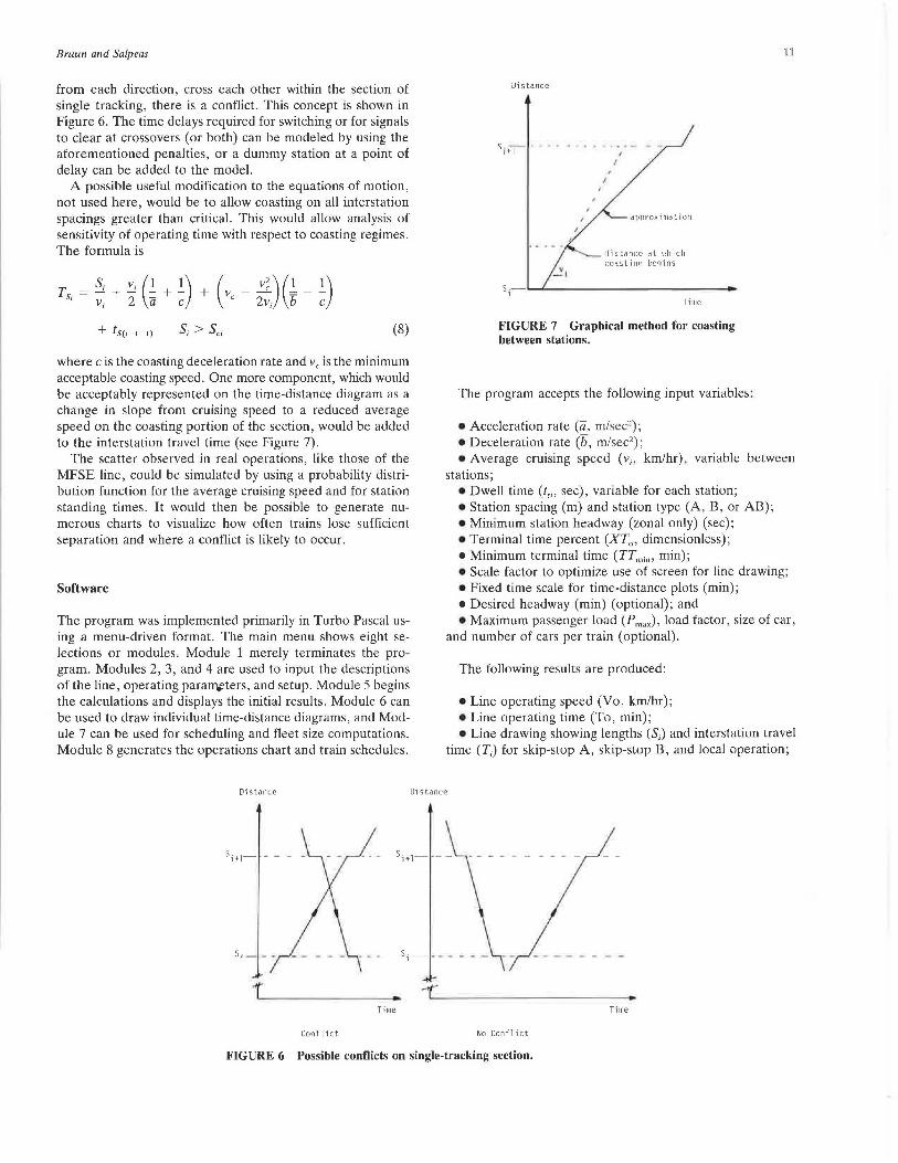
A special operating problem that the model must address is single-tracking conflicts. If two lines on the diagram, one

Bruun and Sa/peas

from each direction, cross each other within the section of single tracking, there is a conflict. This concept is shown in Figure 6. The time delays required for switching or for signals to clear at crossovers (or both) can be modeled by using the aforementioned penalties, or a dummy station at a point of delay can be added to the model.

A possible useful modification to the equations of motion, not used here, would be to allow coasting on all interstation spacings greater than critical. This would allow analysis of sensitivity of operating time with respect to coasting regimes. The formula is

+ lsu + i) (8)

where c is the coasting deceleration rate and v c is the minimum acceptable coasting speed. One more component, which would be acceptably represented on the time-distance diagram as a change in slope from cruising speed to a reduced average speed on the coasting portion of the section, would be added to the interstation travel time (see Figure 7).

The scatter observed in real operations, like those of the MFSE line, could be simulated by using a probability distri­bution function for the average cruising speed and for station standing times. It would then be possible to generate nu­merous charts to visualize how often trains lose sufficient separation and where a conflict is likely to occur.

Software

The program was implemented primarily in Turbo Pascal us­ing a menu-driven format. The main menu shows eight se­lections or modules. Module 1 merely terminates the pro­gram. Modules 2, 3, and 4 are used to input the descriptions of the line, operating param&ters, and setup. Module 5 begins the calculations and displays the initial results. Module 6 can be used to draw individual time-distance diagrams, and Mod­ule 7 can be used for scheduling and fleet size computations. Module 8 generates the operations chart and train schedules.

Oi s ta nee

Time

Conf I ict

Lli s ta nee

s - · .... .. . i+I

~ I

I

I

apnroximation

1iistance rit \.1hicll coastinri bc'lins

Si_..._,,__ ________ ____ __

Tillie

FIGURE 7 Graphical method for coasting between stations.

The program accepts the following input variables:

•Acceleration rate (a, m/sec2);

•Deceleration rate (b , m/sec2);

11

•Average cruising speed (v,, km/hr), variable between stations;

•Dwell time (ts,, sec), variable for each station; •Station spacing (m) and station type (A, B, or AB); •Minimum station headway (zonal only) (sec); •Terminal time percent (XT0 , dimensionless); •Minimum terminal time (TTm;n, min); • Scale factor to optimize use of screen for line drawing; • Fixed time scale for time-distance plots (min); •Desired headway (min) (optional); and •Maximum passenger load (P max), load factor, size of car,

and number of cars per train (optional).

The following results are produced:

•Line operating speed (Vo, km/hr); •Line operating time (To, min); •Line drawing showing lengths (S,) and interstation travel

time (T,) for skip-stop A, skip-stop B, and local operation;

Distance

Time

No Conflict

FIGURE 6 Possible conflicts on single-tracking section.

12

• Operating speed (Vo) and operating time (To) for both zones during zonal operation ;

•The minimum zonal headway (hzmin, min); •Time-distance diagrams for local, skip-stop A, skip-stop

B, or any combination overlaid; and •Time-distance diagram for both zones simultaneously.

The following additional results are available:

• Terminal time based on tt = max {XT0 , TT"''"} (min); •The adjusted cycle time (T,) by rounding Tlh (min); • The adjusted terminal time (11 1 , min); •Number of trains (Ntu) for steady-state operation; and • The required headway (h , min), if P"'"' and other related

parameters are specified.

Each module is briefly described below. Module 2, Rolling Stock Characteristics, is used to input

the acceleration, deceleration, interstation cruising speeds, and station dwell times.

Module 3, Station Spacings and Types, is used to input the distance between stations and the type of station (A, B , or AB) . A line schematic with lengths proportional to intersta­tion distances is drawn as the data are entered.

Module 4, Setup and Default Values, allows for a variety of adjustments, including scaling of the line drawing and plots, choice of operating type, saving and recalling setups, and other options.

Module 5, Travel Times and Spacings, shows the travel time along the line schematic for each spacing as well as the overall operating time and operating speed.

Module 6, Time-Distance Plots, generates the time-distance plots. It is possible to superimpose skip-stop and local op­erations on the same plot. Changing "direction" to "2" in Module 4 will draw the mirror images. When two-zone op­eration is selected, both zones will be plotted together.

Module 7, Scheduling, calculates steady-state fleet size for a given headway and desirable headway for a given passenger flow. Nonclock headways will be neither computed nor per­mitted for any headway greater than 6 min.

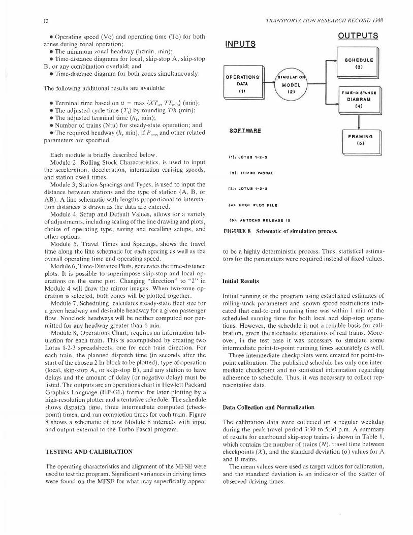
Module 8, Operations Chart, requires an information tab­ulation for each train. This is accomplished by creating two Lotus 1-2-3 spreadsheets, one for each train direction. For each train, the planned dispatch time (in seconds after the start of the chosen 2-hr block to be plotted) , type of operation (local , skip-stop A, or skip-stop 8) , and any station to have delays and the amount of delay (or negative delay) must be listed . The outputs are an operations chart in Hewlett Packard Graphics Language (HP-GL) format for later plotting by a high-resolution plotter and a tentative schedule. The schedule shows dispatch time, three intermediate computed (check­point) times, and run completion times for each train. Figure 8 shows a schematic of how Module 8 interacts with input and output external to the Turbo Pascal program.

TESTING AND CALIBRATION

The operating characteristics and alignment of the MFSE were used to test the program. Significant variances in driving times were found on the MFSE for what may superficially appear

TRANSPORTATION RESEARCH RECORD 1308

INPUTS

OPERATIONS

DATA

(1)

SOFTWARE

(1), LOTUS 1·2-3

f2h TURBO PASCAL

f3) , LOTUS 1·2-3

(•J , HPQL PLOT FILE

15) : AUTOCAD RELEASE 10

FIGURE 8 Schematic of simulation process.

OUTPUTS

SCHEDULE

(3)

TIME-DISTANCE

DIAGRAM

(4)

FRAMING

(6)

to be a highly deterministic process. Thus, statistical estima­tors for the parameters were required instead of fixed values.

Initial Results

Initial running of the program using established estimates of rolling-stock parameters and known speed restrictions indi­cated that end-to-end running time was within 1 min of the scheduled running time for both local and skip-stop opera­tions. However, the schedule is not a reliable basis for cali­bration, given the stochastic operations of real trains. More­over, in the test case it was necessary to simulate some intermediate point-to-point running times accurately as well.

Three intermediate checkpoints were created for point-to­point calibration. The published schedule has only one inter­mediate checkpoint and no statistical information regarding adherence to schedule . Thus , it was necessary to collect rep­resentative data .

Data Collection and Normalization

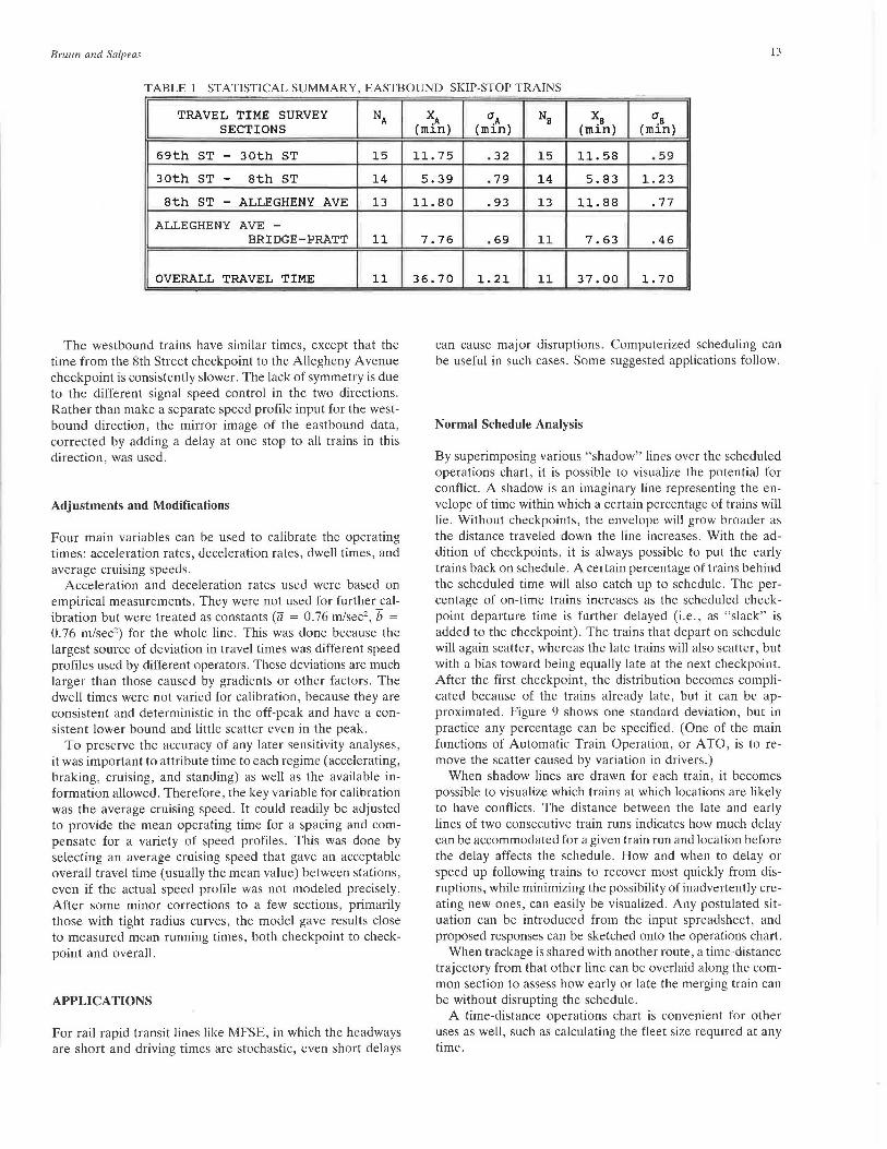
The calibration data were collected on a regular weekday during the peak travel period 3:30 to 5:30 p.m. A summary of results for eastbound skip-stop trains is shown in Table 1, which contains the number of trains (N), travel time between checkpoints (X) , and the standard deviation (rr) values for A and B trains.

The mean values were used as target values for calibration, and the standard deviation is an indicator of the scatter of observed driving times.

Bruun and Sa/peas 13

TABLE 1 STATISTICAL SUMMARY, EASTBOUND SKIP-STOP TRAINS

TRAVEL TIME SURVEY NA SECTIONS

69th ST - 30th ST 15

30th ST - 8th ST 14

8th ST - ALLEGHENY AVE 13

ALLEGHENY AVE -BRIDGE-PRATT 11

OVERALL TRAVEL TIME 11

The westbound trains have similar times, except that the time from the 8th Street checkpoint to the Allegheny Avenue checkpoint is consistently slower. The lack of symmetry is due to the different signal speed control in the two directions. Rather than make a separate speed profile input for the west­bound direction, the mirror image of the eastbound data, corrected by adding a delay at one stop to all trains in this direction, was used.

Adjustments and Modifications

Four main variables can be used to calibrate the operating times: acceleration rates, deceleration rates, dwell times, and average cruising speeds.

Acceleration and deceleration rates used were based on empirical measurements. They were not used for further cal­ibration but were treated as constants (a = 0.76 m/sec2

, b = 0. 76 m/sec2) for the whole line. This was done because the largest source of deviation in travel times was different speed profiles used by different operators. These deviations are much larger than those caused by gradients or other factors. The dwell times were not varied for calibration, because they are consistent and deterministic in the off-peak and have a con­sistent lower bound and little scatter even in the peak.

To preserve the accuracy of any later sensitivity analyses, it was important to attribute time to each regime (accelerating, braking, cruising, and standing) as well as the available in­formation allowed. Therefore, the key variable for calibration was the average cruising speed. It could readily be adjusted to provide the mean operating time for a spacing and com­pensate for a variety of speed profiles. This was done by selecting an average cruising speed that gave an acceptable overall travel time (usually the mean value) between stations, even if the actual speed profile was not modeled precise! y. After some minor corrections to a few sections, primarily those with tight radius curves, the model gave results close to measured mean running times, both checkpoint to check­point and overall.

APPLICATIONS

For rail rapid transit lines like MFSE, in which the headways are short and driving times are stochastic, even short delays

-

XA (min)

GA (min)

NB XB (min)

GB (min)

11. 75 .32 15 11. 58 . 59

5.39 . 79 14 5.83 1. 23

11. 80 .93 13 11. 88 . 77

7.76 . 69 11 7.63 .46

36.70 1. 21 11 37.00 1. 70

can cause major disruptions. Computerized scheduling can be useful in such cases. Some suggested applications follow.

Normal Schedule Analysis

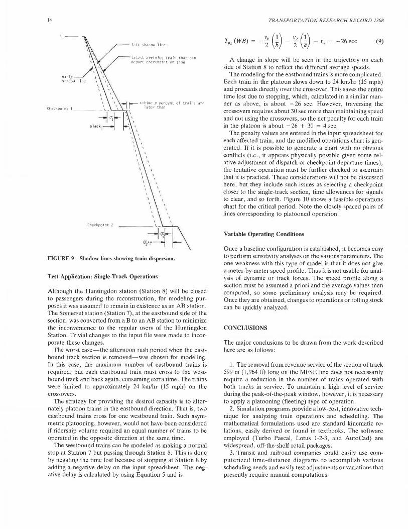
By superimposing various "shadow" lines over the scheduled operations chart, it is possible to visualize the potential for conflict. A shadow is an imaginary line representing the en­velope of time within which a certain percentage of trains will lie. Without checkpoints, the envelope will grow broader as the distance traveled down the line increases. With the ad­dition of checkpoints, it is always possible to put the early trains back on schedule. A certain percentage of trains behind the scheduled time will also catch up to schedule. The per­centage of on-time trains increases as the scheduled check­point departure time is further delayed (i.e., as "slack" is added to the checkpoint). The trains that depart on schedule will again scatter, whereas the late trains will also scatter, but with a bias toward being equally late at the next checkpoint. After the first checkpoint, the distribution becomes compli­cated because of the trains already late, but it can be ap­proximated. Figure 9 shows one standard deviation, but in practice any percentage can be specified. (One of the main functions of Automatic Train Operation, or ATO, is to re­move the scatter caused by variation in drivers.)

When shadow lines are drawn for each train, it becomes possible to visualize which trains at which locations are likely to have conflicts. The distance between the late and early lines of two consecutive train runs indicates how much delay can be accommodated for a given train run and location before the delay affects the schedule. How and when to delay or speed up following trains to recover most quickly from dis­ruptions, while minimizing the possibility of inadvertently cre­ating new ones, can easily be visualized. Any postulated sit­uation can be introduced from the input spreadsheet, and proposed responses can be sketched onto the operations chart.

When trackage is shared with another route, a time-distance trajectory from that other line can be overlaid along the com­mon section to assess how early or late the merging train can be without disrupting the schedule.

A time-distance operations chart is convenient for other uses as well, such as calculating the fleet size required at any time.

14

Q __

Checkpoint Z

late shadow line

latest arrivinq train thJt can depart checkooint on time

FIGURE 9 Shadow lines showing train dispersion.

Test Application: Single-Track Operations

Although the Huntingdon station (Station 8) will be closed to passengers during the reconstruction, for modeling pur­poses it was assumed to remain in existence as an AB station. The Somerset station (Station 7), at the eastbound side of the section, was converted from a B to an AB station to minimize the inconvenience to the regular users of the Huntingdon Station. Trivial changes to the input file were made to incor­porate these changes.

The worst case-the afternoon rush period when the east­bound track section is removed-was chosen for modeling. In this case, the maximum number of eastbound trains is required, but each eastbound train must cross to the west­bound track and back again, consuming extra time. The trains were limited to approximately 24 km/hr (15 mph) on the crossovers.

The strategy for providing the desired capacity is to alter­nately platoon trains in the eastbound direction. That is, two eastbound trains cross for one westbound train. Such asym­metric platooning, however, would not have been considered if ridership volume required an equal number of trains to be operated in the opposite direction at the same time.

The westbound trains can be modeled as making a normal stop at Station 7 but passing through Station 8. This is done by negating the time lost because of stopping at Station 8 by adding a negative delay on the input spreadsheet. The neg­ative delay is calculated by using Equation 5 and is

TRANSPORTATION RESEARCH R ECORD 1308

Tµ 8 (WB) = -~ (~) ~ (~) - t = -26 sec 2u 2a sg (9)

A change in slope will be seen in the trajectory on each side of Station 8 to reflect the different average speeds.

The modeling for the eastbound trains is more complicated. Each train in the platoon slows down to 24 km/hr (15 mph) and proceeds directly over the crossover. This saves the entire time lost due to stopping, which , calculated in a similar man­ner as above, is about - 26 sec. However, traversing the crossovers requires about 30 sec more than maintaining speed and not using the crossovers, so the net penalty for each train in the platoon is about - 26 + 30 = 4 sec.

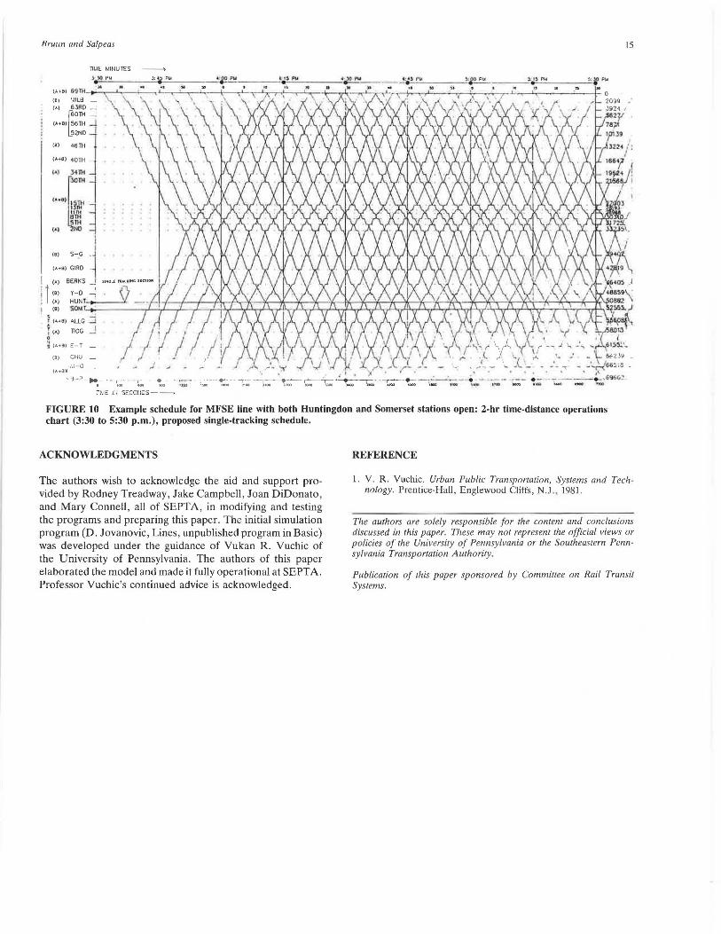
The penalty values are entered in the input spreadsheet for each affected train , and the modified operations chart is gen­erated. If it is possible to generate a chart with no obvious conflicts (i.e., it appears physically possible given some rel­ative adjustment of dispatch or checkpoint departure times), the tentative operation must be further checked to ascertain that it is practical. These considerations will not be discussed here, but they include such issues as selecting a checkpoint closer to the single-track section, time allowances for signals to clear, and so forth. Figure 10 shows a feasible operations chart for the critical period. Note the closely spaced pairs of lines corresponding to platooned operation.

Variable Operating Conditions

Once a baseline configuration is established, it becomes easy to perform sensitivity analyses on the various parameters. The one weakness with this type of model is that it does not give a meter-by-meter speed profile. Thus it is not usable for anal­ysis of dynamic or track forces. The speed profile along a section must be assumed a priori and the average values then computed, so some preliminary analysis may be required. Once they are obtained, changes to operations or rolling stock can be quickly analyzed.

CONCLUSIONS

The major conclusions to be drawn from the work described here are as follows:

1. The removal from revenue service of the section of track 599 m (1,964 ft) long on the MFSE line does not necessarily require a reduction in the number of trains operated with both tracks in service. To maintain a high level of service during the peak-of-the-peak window, however, it is necessary to apply a platooning (fleeting) type of operation.

2. Si111ulaliu11 programs provide a low-cost, innovative tech­nique for analyzing train operations and scheduling. The mathematical formulations used are standard kinematic re­lations, easily derived or found in textbooks . The software employed (Turbo Pascal, Lotus 1-2-3, and AutoCad) are widespread, off-the-shelf retail packages.

3. Transit and railroad companies could easily use com­puterized time-distance diagrams to accomplish various scheduling needs and easily test adjustments or variations that presently require manual computations.

Bruun and Sa/peas

Til.IE MINUTES

.) lO Pt.I

(A+.B) 69fH....-· "~-(Bl ~.l!L8 -(A) 6JRD --'

~OTH --'

::· :::~

:::~:~ ~'81 5TH

(A) 0

(B) S-G

(A+BI CIRO

:-'UE 1:1 SECotliJS - -

15

FIGURE IO Example schedule for MFSE line with both Huntingdon and Somerset stations open: 2-hr time-distance operations chart (3:30 to 5:30 p.m.), proposed single-tracking schedule.

ACKNOWLEDGMENTS

The authors wish to acknowledge the aid and support pro­vided by Rodney Treadway, Jake Campbell, Joan DiDonato, and Mary Connell, all of SEPT A, in modifying and testing the programs and preparing this paper. The initial simulation program (D. Jovanovic, Lines, unpublished program in Basic) was developed under the guidance of Vukan R. Vuchic of the University of Pennsylvania. The authors of this paper elaborated the model and made it fully operational at SEPTA. Professor Vuchic's continued advice is acknowledged.

REFERENCE

1. V. R. Vuchic. Urban Public Transportation, Systems and Tech­nology. Prentice-Hall, Englewood Cliffs, N.J .. 1981.

The authors are solely responsible for the content and conclusions discussed in this paper. These may not represent the official views or policies of the University of Pennsylvania or the Southeastern Penn­sylvania Transportation Authority.

Publication of this paper sponsored by Committee on Rail Transit Systems.