Train and Test Tightness of LP Relaxations inStructured Prediction

Ofer Meshi† Mehrdad Mahdavi† Adrian Weller‡ David Sontag§

Abstract

Structured prediction is used in areas such as computer vision andnatural language processing to predict structured outputs such as seg-mentations or parse trees. In these settings, prediction is performedby MAP inference or, equivalently, by solving an integer linear pro-gram. Because of the complex scoring functions required to obtainaccurate predictions, both learning and inference typically require theuse of approximate solvers. We propose a theoretical explanation tothe striking observation that approximations based on linear program-ming (LP) relaxations are often tight on real-world instances. In par-ticular, we show that learning with LP relaxed inference encouragesintegrality of training instances, and that tightness generalizes fromtrain to test data.

1 Introduction

Many applications of machine learning can be formulated as prediction prob-lems over structured output spaces (Bakir et al., 2007; Nowozin et al., 2014).In such problems output variables are predicted jointly in order to take intoaccount mutual dependencies between them, such as high-order correlationsor structural constraints (e.g., matchings or spanning trees). Unfortunately,the improved expressive power of these models comes at a computationalcost, and indeed, exact prediction and learning become NP-hard in general.

†Toyota Technological Institute at Chicago‡University of Cambridge§New York University

1

Despite this worst-case intractability, efficient approximations often achievevery good performance in practice. In particular, one type of approximationwhich has proved effective in many applications is based on linear program-ming (LP) relaxation. In this approach the prediction problem is first cast asan integer LP (ILP), and then the integrality constraints are relaxed to ob-tain a tractable program. In addition to achieving high prediction accuracy,it has been observed that LP relaxations are often tight in practice. That is,the solution to the relaxed program happens to be optimal for the originalhard problem (an integral solution is found). This is particularly surprisingsince the LPs have complex scoring functions that are not constrained to befrom any tractable family. A major open question is to understand why thesereal-world instances behave so differently from the theoretical worst case.

This paper aims to address this question and to provide a theoreticalexplanation for the tightness of LP relaxations in the context of structuredprediction. In particular, we show that the approximate training objective,although designed to produce accurate predictors, also induces tightness ofthe LP relaxation as a byproduct. Our analysis also suggests that exact train-ing may have the opposite effect. To explain tightness of test instances, weprove a generalization bound for tightness. Our bound implies that if manytraining instances are integral, then test instances are also likely to be inte-gral. Our results are consistent with previous empirical findings, and to ourknowledge provide the first theoretical justification for the wide-spread suc-cess of LP relaxations for structured prediction in settings where the trainingdata is not linearly separable.

2 Related Work

Many structured prediction problems can be represented as ILPs (Roth andYih, 2005; Martins et al., 2009a; Rush et al., 2010). Despite being NP-hard in general (Roth, 1996; Shimony, 1994), various effective approximationshave been proposed. Those include both search-based methods (Daume IIIet al., 2009; Zhang et al., 2014), and natural LP relaxations to the hardILP (Schlesinger, 1976; Koster et al., 1998; Chekuri et al., 2004; Wainwrightet al., 2005). Tightness of LP relaxations for special classes of problems hasbeen studied extensively in recent years and include restricting either thestructure of the model or its score function. For example, the pairwise LPrelaxation is known to be tight for tree-structured models and for super-

2

LP is often tight for structured prediction!Non-Projective Dependency Parsing

*0 John1 saw2 a3 movie4 today5 that6 he7 liked8

*0 John1 saw2 a3 movie4 today5 that6 he7 liked8

Important problem in many languages.

Problem is NP-Hard for all but the simplest models.

For example, in non-projective dependency parsing, we found that the LP relaxation is exact for over 95% of sentences

(Martins et al. ACL ’09, Koo et al., EMNLP ’10)

How often do we exactly solve the problem?

90

92

94

96

98

100

CzeEng

DanDut

PorSlo Swe

Tur

I Percentage of examples where the dual decomposition findsan exact solution.

Language

Percentage of integral solutions

Even when the local LP relaxation is not tight, often still possible to solve exactly and quickly (e.g., Sontag et al. ‘08, Rush & Collins ‘11)

Figure 1: Percentage of integral solutions for dependency parsing from Kooet al. (2010).

modular scores (see, e.g., Wainwright and Jordan, 2008; Thapper and Zivny,2012), and the cycle relaxation (equivalently, the second-level of the Sherali-Adams hierarchy) is known to be tight both for planar Ising models withno external field (Barahona, 1993) and for almost balanced models (Welleret al., 2016). To facilitate efficient prediction, one could restrict the modelclass to be tractable. For example, Taskar et al. (2004) learn supermodularscores, and Meshi et al. (2013) learn tree structures.

However, the sufficient conditions mentioned above are by no means nec-essary, and indeed, many score functions that are useful in practice do notsatisfy them but still produce integral solutions (Roth and Yih, 2004; Sontaget al., 2008; Finley and Joachims, 2008; Martins et al., 2009b; Koo et al.,2010). For example, Martins et al. (2009b) showed that predictors that arelearned with LP relaxation yield integral LPs on 92.88% of the test data ona dependency parsing problem (see Table 2 therein). Koo et al. (2010) ob-served a similar behavior for dependency parsing on a number of languages,as can be seen in Fig. 1 (kindly provided by the authors). The same phe-nomenon has been observed for a multi-label classification task, where testintegrality reached 100% (Finley and Joachims, 2008, Table 3).

Learning structured output predictors from labeled data was proposed invarious forms by Collins (2002); Taskar et al. (2003); Tsochantaridis et al.(2004). These formulations generalize training methods for binary classifiers,such as the Perceptron algorithm and support vector machines (SVMs), tothe case of structured outputs. The learning algorithms repeatedly performprediction, necessitating the use of approximate inference within training as

3

well as at test time. A common approach, introduced right at the inceptionof structured SVMs by Taskar et al. (2003), is to use LP relaxations for thispurpose.

The most closely related work to ours is Kulesza and Pereira (2007),which showed that not all approximations are equally good, and that it isimportant to match the inference algorithms used at train and test time.The authors defined the concept of algorithmic separability which refers tothe setting when an approximate inference algorithm achieves zero loss on adata set. The authors studied the use of LP relaxations for structured learn-ing, giving generalization bounds for the true risk of LP-based prediction.However, since the generalization bounds in Kulesza and Pereira (2007) arefocused on prediction accuracy, the only settings in which tightness on testinstances can be guaranteed are when the training data is algorithmicallyseparable, which is seldom the case in real-world structured prediction tasks(the models are far from perfect). Our paper’s main result (Theorem 4.1),on the other hand, guarantees that the expected fraction of test instancesfor which a LP relaxation is integral is close to that which was estimatedon training data. This then allows us to talk about the generalization ofcomputation. For example, suppose one uses LP relaxation-based algorithmsthat iteratively tighten the relaxation, such as Sontag and Jaakkola (2008);Sontag et al. (2008), and observes that 20% of the instances in the trainingdata are integral using the pairwise relaxation and that after tightening usingcycle constraints the remaining 80% are now integral too. Our generalizationbound then guarantees that approximately the same ratio will hold at testtime (assuming sufficient training data).

Finley and Joachims (2008) also studied the effect of various approximateinference methods in the context of structured prediction. Their theoreticaland empirical results also support the superiority of LP relaxations in thissetting. Martins et al. (2009b) established conditions which guarantee algo-rithmic separability for LP relaxed training, and derived risk bounds for alearning algorithm which uses a combination of exact and relaxed inference.

Finally, recently Globerson et al. (2015) studied the performance of struc-tured predictors for 2D grid graphs with binary labels from an information-theoretic point of view. They proved lower bounds on the minimum achiev-able expected Hamming error in this setting, and proposed a polynomial-timealgorithm that achieves this error. Our work is different since we focus onLP relaxations as an approximation algorithm, we handle the most generalform without making any assumptions on the model or error measure (ex-

4

cept score decomposition), and we concentrate solely on the computationalaspects while ignoring any accuracy concerns.

3 Background

In this section we review the formulation of the structured prediction prob-lem, its LP relaxation, and the associated learning problem. Consider aprediction task where the goal is to map a real-valued input vector x to adiscrete output vector y = (y1, . . . , yn). A popular model class for this taskis based on linear classifiers. In this setting prediction is performed via alinear discriminant rule: y(x;w) = argmaxy′ w

>φ(x, y′), where φ(x, y) ∈ Rd

is a function mapping input-output pairs to feature vectors, and w ∈ Rd isthe corresponding weight vector. Since the output space is often huge (ex-ponential in n), it will generally be intractable to maximize over all possibleoutputs.

In many applications the score function has a particular structure. Specif-ically, we will assume that the score decomposes as a sum of simpler scorefunctions: w>φ(x, y) =

∑cw>c φc(x, yc), where yc is an assignment to a

(non-exclusive) subset of the variables c. For example, it is common touse such a decomposition that assigns scores to single and pairs of out-put variables corresponding to nodes and edges of a graph G: w>φ(x, y) =∑

i∈V (G)w>i φi(x, yi) +

∑ij∈E(G)w

>ijφij(x, yi, yj). Viewing this as a function

of y, we can write the prediction problem as: maxy∑

c θc(yc;x,w) (we willsometimes omit the dependence on x and w in the sequel).

Due to its combinatorial nature, the prediction problem is generally NP-hard. Fortunately, efficient approximations have been proposed. Here wewill be particularly interested in approximations based on LP relaxations.We begin by formulating prediction as the following ILP:1

maxµ∈MLµ∈{0,1}q

∑c

∑yc

µc(yc)θc(yc) +∑i

∑yi

µi(yi)θi(yi) = θ>µ

where ML =

{µ ≥ 0 :

∑yc\i

µc(yc) = µi(yi) ∀c, i ∈ c, yi∑yiµi(yi) = 1 ∀i

}.

Here, µc(yc) is an indicator variable for a factor c and local assignment yc,and q is the total number of factor assignments (dimension of µ). The set

1For convenience we introduce singleton factors θi, which can be set to 0 if needed.

5

ML is known as the local marginal polytope (Wainwright and Jordan, 2008).First, notice that there is a one-to-one correspondence between feasible µ’sand assignments y’s, which is obtained by setting µ to indicators over lo-cal assignments (yc and yi) consistent with y. Second, while solving ILPsis NP-hard in general, it is easy to obtain a tractable program by relax-ing the integrality constraints (µ ∈ {0, 1}q), which may introduce fractionalsolutions to the LP. This relaxation is the first level of the Sherali-Adamshierarchy (Sherali and Adams, 1990), which provides successively tighter LPrelaxations of an ILP. Notice that since the relaxed program is obtained byremoving constraints, its optimal value upper bounds the ILP optimum.

In order to achieve high prediction accuracy, the parameters w are learnedfrom training data. In this supervised learning setting, the model is fit tolabeled examples {(x(m), y(m))}Mm=1, where the goodness of fit is measuredby a task-specific loss ∆(y(x(m);w), y(m)). In the structured SVM (SSVM)framework (Taskar et al., 2003; Tsochantaridis et al., 2004), the empiricalrisk is upper bounded by a convex surrogate called the structured hinge loss,which yields the training objective:2

minw

∑m

maxy

[w>(φ(x(m), y)− φ(x(m), y(m))

)+ ∆(y, y(m))

]. (1)

This is a convex function of w and hence can be optimized in various ways.But, notice that the objective includes a maximization over outputs y for eachtraining example. This loss-augmented prediction task needs to be solved re-peatedly during training (e.g., to evaluate subgradients), which makes train-ing intractable in general. Fortunately, as in prediction, LP relaxation canbe applied to the structured loss (Taskar et al., 2003; Kulesza and Pereira,2007), which yields the relaxed training objective:

minw

∑m

maxµ∈ML

[θ>m(µ− µm) + `>mµ

], (2)

where θm ∈ Rq is a score vector in which each entry represents w>c φc(x(m), yc)

for some c and yc, similarly `m ∈ Rq is a vector with entries3 ∆c(yc, y(m)c ),

and µm is the integral vector corresponding to y(m).

2For brevity, we omit the regularization term, however, all of our results below stillhold with regularization.

3We assume that the task-loss ∆ decomposes as the model score.

6

4 Analysis

In this section we present our main results, proposing a theoretical justifica-tion for the observed tightness of LP relaxations used for inference in modelslearned by structured prediction, both on training and held-out data. Tothis end, we make two complementary arguments: in Section 4.1 we arguethat optimizing the relaxed training objective of Eq. (2) also has the effectof encouraging tightness of training instances; in Section 4.2 we show thattightness generalizes from train to test data.

4.1 Tightness at Training

We first show that the relaxed training objective in Eq. (2), although designedto achieve high accuracy, also induces tightness of the LP relaxation. In orderto simplify notation we focus on a single training instance and drop the indexm. Denote the solutions to the relaxed and integer LPs as:

µL ∈ argmaxµ∈ML

θ>µ µI ∈ argmaxµ∈MLµ∈{0,1}q

θ>µ

Also, let µT be the integral vector corresponding to the ground-truth outputy(m). Now consider the following decomposition:

θ>(µL − µT )relaxed-hinge

= θ>(µL − µI)integrality gap

+ θ>(µI − µT )exact-hinge

(3)

This equality states that the difference in scores between the relaxed optimumand ground-truth (relaxed-hinge) can be written as a sum of the integralitygap and the difference in scores between the exact optimum and the ground-truth (exact-hinge) (notice that all terms are non-negative). This simpledecomposition has several interesting implications.

First, we can immediately derive the following bound on the integralitygap:

θ>(µL − µI) = θ>(µL − µT )− θ>(µI − µT ) (4)

≤ θ>(µL − µT ) (5)

≤ θ>(µL − µT ) + `>µL (6)

≤ maxµ∈ML

(θ>(µ− µT ) + `>µ

), (7)

7

where Eq. (7) is precisely the relaxed training objective from Eq. (2). There-fore, optimizing the approximate training objective of Eq. (2) minimizes anupper bound on the integrality gap. Hence, driving down the approximateobjective also reduces the integrality gap of training instances. One casewhere the integrality gap becomes zero is when the data is algorithmicallyseparable. In this case the relaxed-hinge term vanishes (the exact-hinge mustalso vanish), and integrality is assured.

However, the bound above might sometimes be loose. Indeed, to get thebound we have discarded the exact-hinge term (Eq. (5)), added the task-loss(Eq. (6)), and maximized the loss-augmented objective (Eq. (7)). At thesame time, Eq. (4) provides a precise characterization of the integrality gap.Specifically, the gap is determined by the difference between the relaxed-hingeand the exact-hinge terms. This implies that even when the relaxed-hingeis not zero, a small integrality gap can still be obtained if the exact-hinge isalso large. In fact, the only way to get a large integrality gap is by settingthe exact-hinge much smaller than the relaxed-hinge. But when can thishappen?

A key point is that the relaxed and exact hinge terms are upper boundedby the relaxed and exact training objectives, respectively (the latter addition-ally depend on the task loss ∆). Therefore, minimizing the training objectivewill also reduce the corresponding hinge term (see also Section 5). Usingthis insight, we observe that relaxed training reduces the relaxed-hinge termwithout directly reducing the exact-hinge term, and thereby induces a smallintegrality gap. On the other hand, this also suggests that exact training mayactually increase the integrality gap, since it reduces the exact-hinge withoutalso reducing directly the relaxed-hinge term. This finding is consistent withprevious empirical evidence. Specifically, Martins et al. (2009b, Table 2)showed that on a dependency parsing problem, training with the relaxedobjective achieved 92.88% integral solutions, while exact training achievedonly 83.47% integral solutions. An even stronger effect was observed by Fin-ley and Joachims (2008, Table 3) for multi-label classification, where relaxedtraining resulted in 99.57% integral instances, with exact training attainingonly 17.7% (‘Yeast’ dataset).

In Section 5 we provide further empirical support for our explanation,however, we next also show its possible limitations by providing a counter-example. The counter-example demonstrates that despite training with arelaxed objective, the exact-hinge can in some cases actually be smaller thanthe relaxed-hinge, leading to a loose relaxation. Although this illustrates the

8

limitations of the explanation above, we point out that the correspondinglearning task is far from natural; we believe it is unlikely to arise in real-world applications.

Specifically, we construct a learning scenario where relaxed training ob-tains zero exact-hinge and non-zero relaxed-hinge, so the relaxation is nottight. Consider a model where x ∈ R3, y ∈ {0, 1}3, and the prediction isgiven by:

y(x;w) = argmaxy

(x1y1 + x2y2 + x3y3

+ w [1{y1 6= y2}+ 1{y1 6= y3}+ 1{y2 6= y3}]).

The corresponding LP relaxation is then:

maxµ∈ML

(x1µ1(1) + x2µ2(1) + x3µ3(1) + w[µ12(01) + µ12(10)

+ µ13(01) + µ13(10) + µ23(01) + µ23(10)]).

Next, we construct a trainset where the first instance is: x(1) = (2, 2, 2), y(1) =(1, 1, 0), and the second is: x(2) = (0, 0, 0), y(2) = (1, 1, 0). It can be verifiedthat w = 1 minimizes the relaxed objective (Eq. (2)). However, with thisweight vector the relaxed-hinge for the second instance is equal to 1, whilethe exact-hinge for both instances is 0 (the data is separable w.r.t. w = 1).Consequently, there is an integrality gap of 1 for the second instance, andthe relaxation is loose (the first instance is actually tight).

Finally, note that our derivation above (Eq. (4)) holds for any integral µ,and not just the ground-truth µT . In other words, the only property of µT weare using here is its integrality. Indeed, in Section 5 we verify empirically thattraining a model using random labels still attains the same level of tightnessas training with the ground-truth labels. On the other hand, accuracy dropsdramatically, as expected. This analysis suggests that tightness is not relatedto accuracy of the predictor. Finley and Joachims (2008) explained tightnessof LP relaxations by noting that fractional solutions always incur a loss duringtraining. Our analysis suggests an alternative explanation, emphasizing thedifference in scores (Eq. (4)) rather than the loss, and decoupling tightnessfrom accuracy.

9

4.2 Generalization of Tightness

Our argument in Section 4.1 concerns only the tightness of train instances.However, the empirical evidence discussed above pertains to test data. Tobridge this gap, in this section we show that train tightness implies testtightness. We do so by proving a generalization bound for tightness basedon Rademacher complexity.

We first define a loss function which measures the lack of integrality (or,fractionality) for a given instance. To this end, we consider the discrete setof vertices of the local polytope ML (excluding its convex hull), denotingby MI and MF the sets of fully-integral and non-integral (i.e., fractional)vertices, respectively (so MI ∩ MF = ∅, and MI ∪ MF consists of allvertices of ML). Considering vertices is without loss of generality, sincelinear programs always have a vertex that is optimal. Next, let θx ∈ Rq bethe mapping from weights w and inputs x to scores (as used in Eq. (2)), andlet I∗(θ) = maxµ∈MI θ>µ and F ∗(θ) = maxµ∈MF θ>µ be the best integral andfractional scores attainable, respectively. By convention, we set F ∗(θ) = −∞whenever MF = ∅. The fractionality of θ can be measured by the quantityD(θ) = F ∗(θ)− I∗(θ). If this quantity is large then the LP has a fractionalsolution with a much better score than any integral solution. We can nowdefine the loss:

L(θ) =

{1 D(θ) > 0

0 otherwise. (8)

That is, the loss equals 1 if and only if the optimal fractional solution has a(strictly) higher score than the optimal integral solution.4 Notice that thisloss ignores the ground-truth y, as expected. In addition, we define a ramploss parameterized by γ > 0 which upper bounds the fractionality loss:

ϕγ(θ) =

0 D(θ) ≤ −γ1 +D(θ)/γ −γ < D(θ) ≤ 0

1 D(θ) > 0

, (9)

For this loss to be zero, the best integral solution has to be better thanthe best fractional solution by at least γ, which is a stronger requirementthan mere tightness. In Section 4.2.1 we give examples of models that areguaranteed to satisfy this stronger requirement, and in Section 5 we also show

4Notice that the loss will be 0 whenever the non-integral and integral optima are equal,but this is fine for our purpose, since we consider the relaxation to be tight in this case.

10

this often happens in practice. We point out that ϕγ(θ) is generally hard tocompute, as is L(θ) (due to the discrete optimization involved in computingI∗(θ) and F ∗(θ)). However, here we are only interested in proving thattightness is a generalizing property, so we will not worry about computationalefficiency for now. We are now ready to state the main theorem of thissection.

Theorem 4.1. Let inputs be independently selected according to a probabilitymeasure P (X), and let Θ be the class of all scoring functions θX with ‖w‖2 ≤B. Let ‖φ(x, yc)‖2 ≤ R for all x, c, yc, and q is the total number of factorassignments (dimension of µ). Then for any number of samples M and any0 < δ < 1, with probability at least 1− δ, every θX ∈ Θ satisfies:

EP [L(θX)] ≤ EM [ϕγ(θX)] +O

(q1.5BR

γ√M

)+

√8 ln(2/δ)

M(10)

where EM is the empirical expectation.

Proof. Our proof relies on the following general result from Bartlett andMendelson (2002).

Theorem 4.2 (Bartlett and Mendelson (2002), Theorem 8). Consider a lossfunction L : Y × Θ 7→ [0, 1] and a dominating function ϕ : Y × Θ 7→ [0, 1](i.e., L(y, θ) ≤ ϕ(y, θ) for all y, θ). Let F be a class of functions mappingX to Θ, and let {(x(m), y(m))}Mm=1 be independently selected according to aprobability measure P (x, y). Then for any number of samples M and any0 < δ < 1, with probability at least 1− δ, every f ∈ F satisfies:

E[L(y, f(x))] ≤ EM [ϕ(y, f(x))] +RM (ϕ ◦ f) +

√8 ln(2/δ)

M,

where EM is the empirical expectation, ϕ◦f = {(x, y) 7→ ϕ(y, f(x))−ϕ(y, 0) :f ∈ F}, and RM(F) is the Rademacher complexity of the class F .

To use this result, we define Θ = Rq, f(x) = θx, and F to be the class of all

such functions satisfying ‖w‖2 ≤ B and ‖φ(x, yc)‖2 ≤ R. In order to obtain ameaningful bound, we would like to bound the Rademacher term RM(ϕ◦f).Theorem 12 in Bartlett and Mendelson (2002) states that if ϕ is Lipschitzwith constant L and satisfies ϕ(0) = 0, then RM(ϕ ◦ f) ≤ 2LRM(F). In

addition, Weiss and Taskar (2010) show that RM(F) = O( qBR√M

). Therefore,

it remains to compute the Lipschitz constant of ϕ, which is equal to the Lip-schitz constant of ϕ. For this purpose, we will bound the Lipschitz constant

11

of D(θ), and then use L(ϕγ(θ)) ≤ L(D(θ))/γ (from Eq. (9)).Let µI ∈ argmaxµ∈MI θ>µ and µF ∈ argmaxµ∈MF θ>µ, then:

D(θ1)−D(θ2)

= (µ1F − µ1I) · θ1 − (µ2F − µ2I) · θ2

= (µ1F · θ1 − µ2F · θ2) + (µ2I · θ2 − µ1I · θ1)= (µ1F · θ1 − µ2F · θ2) + (µ1F · θ2 − µ1F · θ2)

+ (µ2I · θ2 − µ1I · θ1) + (µ2I · θ1 − µ2I · θ1)= µ1F · (θ1 − θ2) + (µ1F − µ2F ) · θ2

+ µ2I · (θ2 − θ1) + (µ2I − µ1I) · θ1

≤ (µ1F − µ2I) · (θ1 − θ2) [optimality of µ2F and µ1I ]

≤ ‖µ1F − µ2I‖2‖θ1 − θ2‖2 [Cauchy-Schwarz]

≤ √q‖θ1 − θ2‖2

Therefore, L =√q/γ.

Combining everything together, and dropping the spurious dependenceon y, we obtain the bound in Eq. (10). Finally, we point out that whenusing an L2 regularizer at training, we can actually drop the assumption‖w‖2 ≤ B and instead use a bound on the norm of the optimal solution (asin the analysis of Shalev-Shwartz et al. (2011)).

Theorem 4.1 shows that if we observe high integrality (equivalently, lowfractionality) on a finite sample of training data, then it is likely that in-tegrality of test data will not be much lower, provided sufficient number ofsamples.

Our result actually applies more generally to any two disjoint sets ofvertices, and is not limited to MI and MF . For example, we can replaceMI by the set of vertices with at most 10% fractional values, andMF by therest of the vertices of the local polytope. This gives a different meaning tothe loss D(θ), and the rest of our analysis holds unchanged. Consequently,our generalization result implies that it is likely to observe a similar portionof instances with at most 10% fractional values at test time as we did attraining.

4.2.1 γ-tight relaxations

In this section we study the stronger notion of tightness required by oursurrogate fractionality loss (Eq. (9)), and show examples of models that

12

satisfy it. We use the following definition.

Definition An LP relaxation is called γ-tight if I∗(θ) ≥ F ∗(θ) + γ (soϕγ(θ) = 0). That is, the best integral value is larger than the best non-integral value by at least γ.5

We focus on binary pairwise models and show two cases where the modelis guaranteed to be γ-tight. Proofs are provided in Appendix A. Our firstexample involves balanced models, which are binary pairwise models thathave supermodular scores, or can be made supermodular by “flipping” asubset of the variables (for more details, see Appendix A).

Proposition 4.3. A balanced model with a unique optimum is (α/2)-tight,where α is the difference between the best and second-best (integral) solutions.

This result is of particular interest when learning structured predictorswhere the edge scores depend on the input. Whereas one could learn su-permodular models by enforcing linear inequalities, we know of no tractablemeans of restricting the model to be balanced. Instead, one could learn overthe full space of models using LP relaxation. If the learned models are bal-anced on the training data, Prop. 4.3 together with Theorem 4.1 tell us thatthe pairwise LP relaxation is likely to be tight on test data as well.

Our second example regards models with singleton scores that are muchstronger than the pairwise scores. Consider a binary pairwise model6 inminimal representation, where θi are node scores and θij are edge scoresin this representation (see Appendix A for full details). Further, for eachvariable i, define the set of neighbors with attractive edges N+

i = {j ∈Ni|θij > 0}, and the set of neighbors with repulsive edges N−i = {j ∈ Ni|θij <0}.

Proposition 4.4. If all variables satisfy the condition:

θi ≥ −∑j∈N−i

θij + β, or θi ≤ −∑j∈N+

i

θij − β

for some β > 0, then the model is (β/2)-tight.

Finally, we point out that in both of the examples above, the conditionscan be verified efficiently and if they hold, the value of γ can be computedefficiently.

5Notice that scaling up θ will also increase γ, but our bound in Eq. (10) also growswith the norm of θ (via BR). Therefore, we assume here that ‖θ‖2 is bounded.

6This case easily generalizes to non-binary variables.

13

0 50 100 150 2000

0.5

1Relaxed Training

Relaxed−hingeExact−hingeRelaxed SSVM objExact SSVM obj

0 50 100 150 2000

0.5

1

Training epochs

Train tightnessTest tightnessRelaxed test F

1Exact test F

1

0 50 100 150 200 2500

0.5

1

1.5Exact Training

Training epochs0 50 100 150 200 250

0

0.5

1

−0.4 −0.2 00

100

200

Relaxed Training

−0.4 −0.2 00

100

200

Exact Training

I*−F*

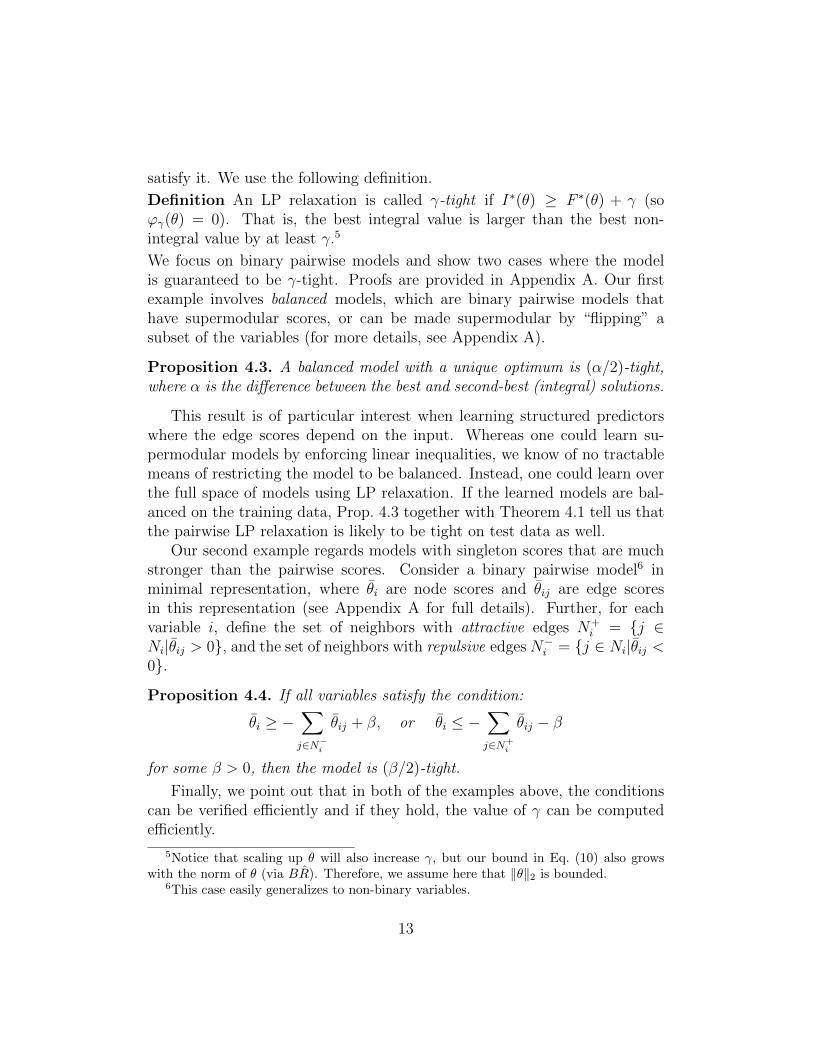
Figure 2: Training with the ‘Yeast’ dataset. Various quantities of interest areshown as a function of training iterations. (Left) Training with LP relaxation.(Middle) Training with ILP. (Right) Integrality margin (bin widths are scaleddifferently).

5 Experiments

In this section we present some numerical results to support our theoreticalanalysis. We run experiments for both a multi-label classification task andan image segmentation task. For training we have implemented the block-coordinate Frank-Wolfe algorithm for structured SVM (Lacoste-Julien et al.,2013), using GLPK as the LP solver.7 In all of our experiments we use astandard L2 regularizer, chosen via cross-validation.

Multi-label classification For multi-label classification we adopt the ex-perimental setting of Finley and Joachims (2008). In this setting labels arerepresented by binary variables, the model consists of singleton and pairwisefactors forming a fully connected graph over the labels, and the task loss isthe normalized Hamming distance.

Fig. 2 shows relaxed and exact training iterations for the ‘Yeast’ dataset(14 labels). We plot the relaxed and exact hinge terms (Eq. (3)), the exactand relaxed SSVM training objectives8 (Eq. (1) and Eq. (2), respectively),fraction of train and test instances having integral solutions, as well as testaccuracy (measured by F1 score). Whenever a fractional solution was foundwith relaxed inference, a simple rounding scheme was applied to obtain a valid

7http://www.gnu.org/software/glpk8The displayed objective values are averaged over train instances and exclude regular-

ization.

14

0 100 200 300 400 5000

0.5

1Relaxed Training

Relaxed−hingeExact−hingeRelaxed SSVM objExact SSVM obj

0 100 200 300 400 5000

0.5

1

Training epochs

Train tightnessTest tightnessRelaxed test F

1Exact test F

1

0 50 100 150 200 250 3000

0.5

1Exact Training

Training epochs0 50 100 150 200 250 300

0

0.5

1

−0.2 0 0.2 0.4 0.60

100

200

300

Relaxed Training

−0.2 0 0.2 0.4 0.60

100

200

300

Exact Training

I*−F*

Figure 3: Training with the ‘Scene’ dataset. Various quantities of interest areshown as a function of training iterations. (Left) Training with LP relaxation.(Middle) Training with ILP. (Right) Integrality margin.

prediction. First, we note that the relaxed-hinge values are nicely correlatedwith the relaxed training objective, and likewise the exact-hinge is correlatedwith the exact objective (left and middle, top). Second, observe that withrelaxed training, the relaxed-hinge and the exact-hinge are very close (left,top), so the integrality gap, given by their difference, remains small (almost0 here). On the other hand, with exact training the exact-hinge is reducedmuch more than the relaxed-hinge, which results in a large integrality gap(middle, top). Indeed, we can see that the percentage of integral solutionsis almost 100% for relaxed training (left, bottom), and close to 0% withexact training (middle, bottom). To get a better understanding, we showa histogram of the difference between the optimal integral and fractionalvalues, i.e., the integrality margin (I∗(θ) − F ∗(θ)), under the final learnedmodel for all training instances (right). It can be seen that with relaxedtraining this margin is positive (although small), while exact training resultsin larger negative values. Third, we notice that train and test integralitylevels are very close to each other, almost indistinguishable (left and middle,bottom), which provides some empirical support to our generalization resultfrom Section 4.2.

We next train a model using random labels (with similar label counts asthe true data). In this setting the learned model obtains 100% tight traininginstances (not shown), which supports our claim that any integral solutioncan be used in place of the ground-truth, and that accuracy is not importantfor tightness. Finally, in order to verify that tightness is not coincidental,

15

we tested the tightness of the relaxation induced by a random weight vectorw. We found that random models are never tight (in 20 trials), which showsthat tightness of the relaxation does not come by chance.

We now proceed to perform experiments on the ‘Scene’ dataset (6 labels).The results, in Fig. 3, are quite similar to the ‘Yeast’ results, except forthe behavior of exact training (middle) and the integrality margin (right).Specifically, we observe that in this case the relaxed-hinge and exact-hingeare close in value (middle, top), as for relaxed training (left, top). As aconsequence, the integrality gap is very small and the relaxation is tightfor almost all train (and test) instances. These results show that sometimesoptimizing the exact objective can reduce the relaxed objective (and relaxed-hinge) as well. Further, in this setting we observe a larger integrality margin(right), which means that the integral optimum is strictly better than thefractional one.

We conjecture that the LP instances are easy in this case due to thedominance of the singleton scores.9 Specifically, the features provide a strongsignal which allows label assignment to be decided mostly based on the localscore, with little influence coming from the pairwise terms. To test thisconjecture we repeat the experiment while injecting Gaussian noise into theinput features, forcing the model to rely more on the pairwise interactions.We find that with the noisy singleton scores the results are indeed similarto the ‘Yeast’ dataset, where a large integrality gap is observed and fewerinstances are tight (see Appendix B in the supplement).

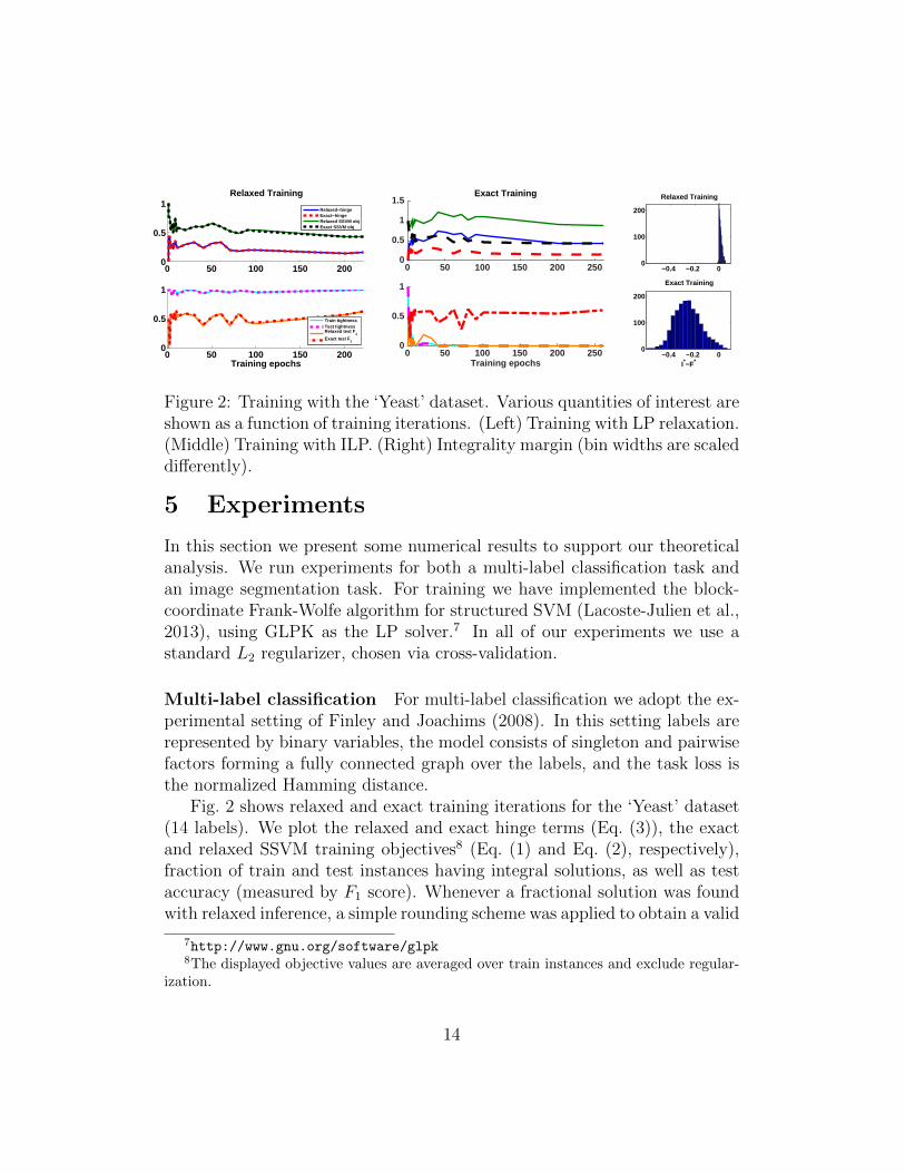
Image segmentation Finally, we conduct experiments on a foreground-background segmentation problem using the Weizmann Horse dataset (Boren-stein et al., 2004). The data consists of 328 images, of which we use the first50 for training and the rest for testing. Here a binary output variable is as-signed to each pixel, and there are ∼ 58K variables per image on average. Weextract singleton and pairwise features as described in Domke (2013). Fig. 4shows the same quantities as in the multi-label setting, except for the accu-racy measure – here we compute the percentage of correctly classified pixelsrather than F1. We observe a very similar behavior to that of the ‘Scene’multi-label dataset (Fig. 3). Specifically, both relaxed and exact trainingproduce a small integrality gap and high percentage of tight instances. Un-

9With ILP training, the condition in Prop. 4.4 is satisfied for 65% of all variables,although only 1% of the training instances satisfy it for all their variables.

16

0 200 400 600 800 10000

1

2

3x 10

4 Relaxed Training

Relaxed−hingeExact−hingeRelaxed SSVM objExact SSVM obj

0 200 400 600 800 10000

0.5

1

Training epochs

Train tightnessTest tightnessRelaxed test accuracyExact test accuracy

0 200 400 600 800 10000

1

2

3x 10

4 Exact Training

0 200 400 600 800 10000

0.5

1

Training epochs

Figure 4: Training for foreground-background segmentation with the Weiz-mann Horse dataset. Various quantities of interest are shown as a functionof training iterations. (Left) Training with LP relaxation. (Right) Trainingwith ILP.

like the ‘Scene’ dataset, here only 1.2% of variables satisfy the condition inProp. 4.4 (using LP training). In all of our experiments the learned modelscores were never balanced (Prop. 4.3), although for the segmentation prob-lem we believe the models learned are close to balanced, both for relaxed andexact training.

6 Conclusion

In this paper we propose an explanation for the tightness of LP relaxationswhich has been observed in many structured prediction applications. Ouranalysis is based on a careful examination of the integrality gap and its re-lation to the training objective. It shows how training with LP relaxations,although designed with accuracy considerations in mind, also induces tight-ness of the relaxation. Our derivation also suggests that exact training maysometimes have the opposite effect, increasing the integrality gap.

To explain tightness of test instances, we show that tightness general-izes from train to test instances. Compared to the generalization bound ofKulesza and Pereira (2007), our bound only considers the tightness of the in-stance, ignoring label errors. Thus, for example, if learning happens to settleon a set of parameters in a tractable regime (e.g., supermodular potentialsor stable instances (Makarychev et al., 2014)) for which the LP relaxation

17

is tight for all training instances, our generalization bound guarantees thatwith high probability the LP relaxation will also be tight on test instances. Incontrast, in Kulesza and Pereira (2007)’s bound, tightness on test instancescan only be guaranteed when the training data is algorithmically separable(i.e., LP-relaxed inference predicts perfectly).

Our work suggests many directions for further study. Our analysis inSection 4.1 focuses on the score hinge and ignores the task loss ∆. It wouldbe interesting to further study the effect of various task losses on tightnessof the relaxation at training. Next, our bound in Section 4.2 is intractableto compute due to the hardness of the surrogate loss ϕ. It is thereforedesirable to derive a tractable alternative which could be used to obtaina useful guarantee in practice. The upper bound on integrality shown inSection 4.1 holds for other convex relaxations which have been proposed forstructured prediction, such as semi-definite programming relaxations (Kumaret al., 2009). However, it is less clear how to extend the generalization resultto such non-polyhedral relaxations. Finally, we hope that our methodologywill be useful for shedding light on tightness of convex relaxations in otherlearning problems.

Appendix

A γ-Tight LP Relaxations

In this section we provide full derivations for the results in Section 4.2.1.We make extensive use of the results in Weller et al. (2016) (some of whichare restated here for completeness). We start by defining a model in mini-mal representation, which will be convenient for the derivations that follow.Specifically, in the case of binary variables (yi ∈ {0, 1}) with pairwise fac-tors, we define a value ηi for each variable, and a value ηij for each pair. Themapping between the over-complete vector µ and the minimal vector η is asfollows. For singleton factors, we have:

µi =

(1− ηiηi

)Similarly, for the pairwise factors, we have:

µij =

(1 + ηij − ηi − ηj ηj − ηij ,

ηi − ηij ηij

)18

The corresponding mapping to minimal parameters is then:

θi = θi(1)− θi(0) +∑j∈Ni

(θij(1, 0)− θij(0, 0))

θij = θij(1, 1) + θij(0, 0)− θij(0, 1)− θij(1, 0)

In this representation, the LP relaxation is given by (up to constants):

maxη∈L

f(η) :=n∑i=1

θiηi +∑ij∈E

θijηij

where L is the appropriate transformation of ML to the equivalent reducedspace of η:

0 ≤ ηi ≤ 1 ∀imax(0, ηi + ηj − 1) ≤ ηij ≤ min(ηi, ηj) ∀ij ∈ E

If θij > 0 (θij < 0), then the edge is called attractive (repulsive). If alledges are attractive, then the LP relaxation is known to be tight (Wainwrightand Jordan, 2008). When not all edges are attractive, in some cases it ispossible to make them attractive by flipping a subset of the variables (yi ←1− yi).10 In such cases the model is called balanced.

In the sequel we will make use of the known fact that all vertices of thelocal polytope are half-integral (take values in {0, 1

2, 1}) (Wainwright and

Jordan, 2008). We are now ready to prove the propositions (restated herefor convenience).

A.1 Proof of Proposition 4.3

Proposition 4.3 A balanced model with a unique optimum is (α/2)-tight,where α is the difference between the best and second-best (integral) solu-tions.

Proof. Weller et al. (2016) define for a given variable i the function F iL(z),

which returns for every 0 ≤ z ≤ 1 the constrained optimum:

F iL(z) = max

η∈Lηi=z

f(η)

10The flip-set, if exists, is easy to find by making a single pass over the graph (see Weller(2015) for more details).

19

Given this definition, they show that for a balanced model, F iL(z) is a linear

function (Weller et al., 2016, Theorem 6).Let m be the optimal score, let η1 be the unique optimum integral vertex

in minimal form so f(η1) = m, and any other integral vertex has valueat most m − α. Denote the state of η1 at coordinate i by z∗ = η1i , andconsider computing the constrained optimum holding ηi to various states.By assumption, any other integral vertex has value at most m−α, therefore,

F iL(z∗) = m

F iL(1− z∗) ≤ m− α

(the second line holds with equality if there exists a second-best solution η2

s.t. η2i 6= η1i ). Since F iL(z) is a linear function, we have that:

F iL(1/2) ≤ m− α/2 (11)

Next, towards contradiction, suppose that there exists a fractional vertexηf with value f(ηf ) > m− α/2. Let j be a fractional coordinate, so ηfj = 1

2

(since vertices are half-integral). Our assumption implies that F jL(1/2) >

m − α/2, but this contradicts Eq. (11). Therefore, we conclude that anyfractional solution has value at most f(ηf ) ≤ m− α/2.

It is possible to check in polynomial time if a model is balanced, if ithas a unique optimum, and compute α. This can be done by computing thedifference in value to the second-best. In order to find the second-best: onecan constrain each variable in turn to differ from the state of the optimalsolution, and recompute the MAP solution; finally, take the maximum overall these trials.

A.2 Proof of Proposition 4.4

Proposition 4.4 If all variables satisfy the condition:

θi ≥ −∑j∈N−i

θij + β, or θi ≤ −∑j∈N+

i

θij − β

for some β > 0, then the model is (β/2)-tight.

20

Proof. For any binary pairwise models, given singleton terms {ηi}, the opti-mal edge terms are given by (for details see Weller et al., 2016):

ηij(ηi, ηj) =

{min(ηi, ηj) if θij > 0

max(0, ηi + ηj − 1) if θij < 0

Now, consider a variable i and let Ni be the set of its neighbors in the graph.Further, define the sets N+

i = {j ∈ Ni|θij > 0} and N−i = {j ∈ Ni|θij < 0},corresponding to attractive and repulsive edges, respectively. We next focuson the parts of the objective affected by the value at ηi (recomputing optimaledge terms); recall that all vertices are half-integral:

ηi = 1 ηi = 1/2 ηi = 0

θi +∑

j∈N+i

ηj=1

θij + 12

∑j∈N+

i

ηj=12

θij +∑

j∈N−iηj=1

θij + 12

∑j∈N−iηj=

12

θij12 θi + 1

2

∑j∈N+

i

ηj∈{ 12 ,1}

θij + 12

∑j∈N−iηj=1

θij 0

It is easy to verify that the condition θi ≥ −∑

j∈N−iθij + β guarantees that

ηi = 1 in the optimal solution. We next bound the difference in objectivevalues resulting from setting ηi = 1/2.

∆f =1

2

θi +∑j∈N+

iηj=1

θij +∑j∈N−i

ηj∈{ 12 ,1}

θij

≥ 1

2

θi +∑j∈N−i

θij

≥ β/2

Similarly, when θi ≤ −∑

j∈N+iθij−β, then ηi = 0 in any optimal solution.

The difference in objective values from setting ηi = 1/2 in this case is:

∆f = −1

2

θi +∑j∈N+

i

ηj∈{ 12 ,1}

θij +∑j∈N−iηj=1

θij

≥ −1

2

θi +∑j∈N+

i

θij

≥ β/2

Notice that for more fractional coordinates the difference in values canonly increase, so in any case the fractional solution is worse by at leastβ/2.

21

0 1000 2000 3000 40000

0.5

1Relaxed Training

Relaxed−hingeExact−hingeRelaxed SSVM objExact SSVM obj

0 1000 2000 3000 40000

0.5

1

Training epochs

Train tightnessTest tightnessRelaxed test F

1Exact test F

1

0 1000 2000 3000 40000

0.5

1Exact Training

0 1000 2000 3000 40000

0.5

1

Training epochs

−1 0 10

200

400

600Relaxed Training

−1 0 10

200

400

600Exact Training

I*−F*

Figure 5: Training with a noisy version of the ‘Scene’ dataset. Variousquantities of interest are shown as a function of training iterations. (Left)Training with LP relaxation. (Middle) Training with ILP. (Right) Integralitymargin (bin widths are scaled differently).

B Additional Experimental Results

In this section we present additional experimental results for the ‘Scene’dataset. Specifically, we inject random Gaussian noise to the input featuresin order to reduce the signal in the singleton scores and increase the role ofthe pairwise interactions. This makes the problem harder since the predictionneeds to account for global information.

In Fig. 5 we observe that with exact training the exact loss is minimized,causing the exact-hinge to decrease, since it is upper bounded by the loss(middle, top). On the other hand, the relaxed-hinge (and relaxed loss) in-crease during training, which results in a large integrality gap and fewer tightinstances. In contrast, with relaxed training the relaxed loss is minimized,which causes the relaxed-hinge to decrease. Since the exact-hinge is upperbounded by the relaxed-hinge it also decreases, but both hinge terms de-crease similarly and remain very close to each other. This results in a smallintegrality gap and tightness of almost all instances.

Finally, in contrast to other settings, in Fig. 5 we observe that with exacttraining the test tightness is noticeably higher (about 20%) than the traintightness (Fig. 5, middle, bottom). This does not contradict our boundfrom Theorem 4.1, since in fact the test fractionality is even lower than thebound suggests. On the other hand, this result does entail that train andtest tightness may sometimes behave differently, which means that we mightneed to increase the size of the trainset in order to get a tighter bound.

22

ReferencesG. H. Bakir, T. Hofmann, B. Scholkopf, A. J. Smola, B. Taskar, and S. V. N.

Vishwanathan. Predicting Structured Data. The MIT Press, 2007.

F. Barahona. On cuts and matchings in planar graphs. Mathematical Program-ming, 60:53–68, 1993.

P. L. Bartlett and S. Mendelson. Rademacher and gaussian complexities: Riskbounds and structural results. The Journal of Machine Learning Research, 3:463–482, 2002.

E. Borenstein, E. Sharon, and S. Ullman. Combining top-down and bottom-upsegmentation. In CVPR, 2004.

C. Chekuri, S. Khanna, J. Naor, and L. Zosin. A linear programming formulationand approximation algorithms for the metric labeling problem. SIAM J. onDiscrete Mathematics, 18(3):608–625, 2004.

M. Collins. Discriminative training methods for hidden Markov models: Theoryand experiments with perceptron algorithms. In EMNLP, 2002.

H. Daume III, J. Langford, and D. Marcu. Search-based structured prediction.Machine Learning, 75(3):297–325, 2009.

J. Domke. Learning graphical model parameters with approximate marginal in-ference. Pattern Analysis and Machine Intelligence, IEEE Transactions on, 35(10), 2013.

T. Finley and T. Joachims. Training structural SVMs when exact inference isintractable. In Proceedings of the 25th International Conference on Machinelearning, pages 304–311, 2008.

A. Globerson, T. Roughgarden, D. Sontag, and C. Yildirim. How hard is inferencefor structured prediction? In ICML, 2015.

T. Koo, A. M. Rush, M. Collins, T. Jaakkola, and D. Sontag. Dual decompositionfor parsing with non-projective head automata. In EMNLP, 2010.

A. Koster, S. van Hoesel, and A. Kolen. The partial constraint satisfaction prob-lem: Facets and lifting theorems. Operations Research Letters, 23:89–97, 1998.

A. Kulesza and F. Pereira. Structured learning with approximate inference. InAdvances in Neural Information Processing Systems 20, pages 785–792. 2007.

M. P. Kumar, V. Kolmogorov, and P. H. S. Torr. An analysis of convex relaxationsfor MAP estimation of discrete MRFs. JMLR, 10:71–106, 2009.

S. Lacoste-Julien, M. Jaggi, M. Schmidt, and P. Pletscher. Block-coordinate Frank-Wolfe optimization for structural SVMs. In ICML, pages 53–61, 2013.

23

K. Makarychev, Y. Makarychev, and A. Vijayaraghavan. Bilulinial stable instancesof max cut and minimum multiway cut. Proc. 22nd Symposium on DiscreteAlgorithms (SODA), 2014.

A. Martins, N. Smith, and E. P. Xing. Concise integer linear programming formu-lations for dependency parsing. In ACL, 2009a.

A. Martins, N. Smith, and E. P. Xing. Polyhedral outer approximations withapplication to natural language parsing. In Proceedings of the 26th InternationalConference on Machine Learning, 2009b.

O. Meshi, E. Eban, G. Elidan, and A. Globerson. Learning max-margin treepredictors. In UAI, 2013.

S. Nowozin, P. V. Gehler, J. Jancsary, and C. Lampert. Advanced StructuredPrediction. MIT Press, 2014.

D. Roth. On the hardness of approximate reasoning. Artificial Intelligence, 82,1996.

D. Roth and W. Yih. A linear programming formulation for global inference innatural language tasks. In CoNLL, The 8th Conference on Natural LanguageLearning, 2004.

D. Roth and W. Yih. Integer linear programming inference for conditional randomfields. In ICML, pages 736–743. ACM, 2005.

A. M. Rush, D. Sontag, M. Collins, and T. Jaakkola. On dual decomposition andlinear programming relaxations for natural language processing. In EMNLP,2010.

M. I. Schlesinger. Syntactic analysis of two-dimensional visual signals in noisyconditions. Kibernetika, 4:113–130, 1976.

S. Shalev-Shwartz, Y. Singer, N. Srebro, and A. Cotter. Pegasos: Primal estimatedsub-gradient solver for svm. Mathematical programming, 127(1):3–30, 2011.

H. D. Sherali and W. P. Adams. A hierarchy of relaxations between the continuousand convex hull representations for zero-one programming problems. SIAM J.on Disc. Math., 3(3):411–430, 1990.

Y. Shimony. Finding the MAPs for belief networks is NP-hard. Aritifical Intelli-gence, 68(2):399–410, 1994.

D. Sontag and T. Jaakkola. New outer bounds on the marginal polytope. InJ. Platt, D. Koller, Y. Singer, and S. Roweis, editors, Advances in Neural Infor-mation Processing Systems 20, pages 1393–1400. MIT Press, Cambridge, MA,2008.

D. Sontag, T. Meltzer, A. Globerson, T. Jaakkola, and Y. Weiss. Tightening LPrelaxations for MAP using message passing. In UAI, pages 503–510, 2008.

24

B. Taskar, C. Guestrin, and D. Koller. Max-margin Markov networks. In Advancesin Neural Information Processing Systems. MIT Press, 2003.

B. Taskar, V. Chatalbashev, and D. Koller. Learning associative Markov networks.In Proc. ICML. ACM Press, 2004.

J. Thapper and S. Zivny. The power of linear programming for valued CSPs. InFOCS, 2012.

I. Tsochantaridis, T. Hofmann, T. Joachims, and Y. Altun. Support vector ma-chine learning for interdependent and structured output spaces. In ICML, pages104–112, 2004.

M. Wainwright and M. I. Jordan. Graphical Models, Exponential Families, andVariational Inference. Now Publishers Inc., Hanover, MA, USA, 2008.

M. Wainwright, T. Jaakkola, and A. Willsky. MAP estimation via agreement ontrees: message-passing and linear programming. IEEE Transactions on Infor-mation Theory, 51(11):3697–3717, 2005.

D. Weiss and B. Taskar. Structured Prediction Cascades. In AISTATS, 2010.

A. Weller. Bethe and related pairwise entropy approximations. In Uncertainty inArtificial Intelligence (UAI), 2015.

A. Weller, M. Rowland, and D. Sontag. Tightness of LP relaxations for almostbalanced models. In AISTATS, 2016.

Y. Zhang, T. Lei, R. Barzilay, and T. Jaakkola. Greed is good if randomized: Newinference for dependency parsing. In EMNLP, 2014.

25