TRAFFIC PROJECTION AND ASSIGNMENT

RESEARCH REPORT 119-3F Final Report

by

Vergil G. Stover Study Supervisor

and

J. D. Benson Assistant Research Planner

Prepared in cooperation with the Texas Highway Department

and the U. S. Department of Transportation, Federal Highway Administration

Study No. 2-10-68-119

Texas Transportation Institute Texas A&M University

College Station, Texas

September 1971

TABLE OF CONTENTS

ABSTRACT . • . . . • • . . ." . . • • . . • • • • . • • • • • • • ii

SUJ:-1}1A.RY . . . . • . . • • . • . . • • . . . . • • . • • • • • • • iii

IMPLEMENTATION STATEMENT . . . • • . • . •. • • • • • . • • • . • iv

INTRODUCTION • •

Significant Accomplishments •

SUMMARY OF STUDY ACTIVITIES .•••

Traffic Assignment Packages •

Trip Distribution . • . • •

Other Computer Programming .•

Accuracy of Employment and Non-Home Trip Ends from Home Interviews .••

Accuracy of All-Or-Nothing Assignments in Estimating Turn Movements •••.• ·

One-Hundred Percent Home Interview Data .

APPENDIX • • . . • . . . . •

1

2

3

3

6

18

19

38

46

68

The opinions, findings, and conclusions expressed in this publication

are those of the authors and are not necessarily those of the Federal

Highway Administration.

i

ABSTRACT

Two traffic assignment packages were developed for use on the Texas

Highway Department's IBM 360/50 Computer System. The Texas Small Network

Package, which will accommodate small networks of up to 4,000 nodes,

implements a new algorithm which allows the trees to be built and the

network simultaneously loaded. The Texas Large Network Package, which

will accommodate a network of up to about 16,000 nodes, uses a new minimum

path algorithm which is considerably more efficient than any previously

used. A battery of computer programs for trip distribution was also

developed and adopted by the Texas Highway Department.

The accuracy of employment and non-home trip ends from home interviews

was investigated. The accuracy of all-or-nothing traffic assignments

in estimating turn movements was also investigated.

Home interviews were conducted by the Texas Highway Department in

100 percent of the dwelling units in three adjacent zones in San Antonio.

A preliminary analysis of the 100 percent data indicates that very high

sampling rates are necessary in order to estimate the number of trips with

a small confidence limit.

Key words: Traffic assignment, trip distribution, trip generation,

accuracy in estimating trip-ends.

ii

SUMHARY

Two traffic assignment packages were developed for use on the Texas

Highway Department's IBM 360/50 Computer System. The Texas Small Network

Package (see Research Report 119-1), which will accommodate a network

of up to 4,000 nodes, implements a new algorithm which allows the trees

to be built and the network simultaneously loaded. The Texas Large

Network Package (see Research Report 119-2), which will accommodate a

network of up to about 16,000 nodes, uses a new minimum path algorithm

which is considerably more efficient than any previously used.

A battery of computer programs for trip distribution was developed

and adopted by the Texas Highway Department. This package has the

capability of performing several different types of trip distributions

including distributions using a newly developed constrained interactarice

model.

The accuracy of employment and non-home trip ends from home interviews

was investigated. Three methods for estimating employment were compared.

It was concluded that the origin-destination survey does not yield

an acceptable estimate of the employment for zones, districts,

or census tracts. The accuracy of ali-or-nothing traffic assignments

in estimating turn movements was also investigated.

Home interviews were conducted by the Texas Highway Department in

100 percent of the dwelling units in three adjacent zones in San Antonio.

An analysis of the 100 percent data was initiated. The preliminary

results of this analysis indicate that unexpectedly high sampling rates

would be needed in order to estimate the total number of trip ends with

desirable accuracy.

iii

IMPLEMENTATION STATEMENT

The Texas Large Network Package, the Texas Small Network Package,

and the Texas Trip Distribution Package have been adopted by the Texas

Highway Department and are currently being used in their urban transportation

studies.

The results of the analysis of the accuracy of horne interview data

in estimating employment and non-horne trip ends and the results of the

preliminary analysis of the 100 percent data from San Antonio were used

by the Texas Highway Department as the basis for their decision to

abandon the traditional origin-destination survey and perform a "synthetic"

urban transportation study for the Houston-Galveston area.

INTRODUCTION

Study Number 2-10-68-119 is a component of the continuing cooperative

research effort between the Texas Transportation Institute and the Texas

Highway Department. This three-year study was based upon research previously

conducted under Study Number 2-8-63-60 and continued a number of research

elements undertaken but not completed under this previous study. It also

interfaces with Study Number 2-10-71-167 which began September 1, 1970;

a number of research elements initiated under Study 119 are to be completed

in this follow-on study.

The primary concern of Study Number 2-10-68-119 (as with its predecessor

and follow-on studies) was to provide technical support for the continuing

activities of the Texas Highway Department in the conduct of the several

urban transportation studies throughout the State of Texas. Therefore,

the project objectives were formulated and a work program was executed

so as to be of maximum value in the conduct of the several urban transporta­

tion studies in the State. Since the project was to be attuned to the

day-to-day performance of urban transportation studies, the study was funded

and administered as a planning study rather than research study.

The close liaison between the research staff and personnel of the

Planning-Survey Division of the Texas Highway Department throughout the

course of the study was an essential ingredient. Through this contact,

the research staff was continually aware of the operational problems and

practices of the Highway Department. Similarly, the operational staff

was involved in the research, development and evaluation from the time work

1

on individual tasks was initiated. This relationship has led to exception-

ally high implementation and utilization of the study findings; in most

instances research findings were applied and used in the Highway Department's

operation well before drafts of the reports were developed. Indeed, most

of those activities carried over into Study Number 2-10-71-167 involved the

preparation of reports concerning the development and evaluation of

procedures which have been adopted and ~omputer programs which are in

use by the Texas Highway Department.

Significant Accomplishments

The more important accomplishments under this study are:

1. The Texas Highway Planning Survey Division was provided with such support that normal operational activities relative to the processing of Urban Transportation study data were maintained with almost no disruption during the changeover from the IBM 7094 to the IBM 360/50 computer.

2. A traffic assignment package which will accomodate a network ~p to 4,000 nodes and which will operate in the normal job stream was developed for the Texas Highway Department. This package was based upon a new algorithm which allows trees to be built and the network simultaneously loaded; in addition to being convenient this procedure is exceptionally fast.

3. A new m1n1mum path algorithm, which is considerably more efficient than any previously used, was developed and incorporated into a traffic assignment package for large networks (up to approximately 16,000 nodes).

4. The Texas Highway Department was able to continue processing urban transportation study data and to make assignments to networks already coded without the necessity for expensive and time consuming re-ceding of networks for disruptive changes in procedures.

5. A battery of computer programs for trip distribution was developed and adopted by the Texas Highway Department.

2

SUMMARY OF STUDY ACTIVITIES

A primary activity conducted under Study 2-10-68-119 was to maintain

operational capability on the part of the Texas Highway Department in the

conduct of on-going urban transportation studies. The importance of this

activity was dictated by the changeover from the IBM 7094 to the IBM 360

computer during the term of the study.

A second major activity was the development of a computerized

trip distribution procedure that would avoid the extensive man-hour •

requirements of the manual Texas Pattern Trip Procedure while avoiding the

shortcomings of the conventional gravity model. These and other study

activities are summarized in the following sections.

Traffic Assignment Packages

The development and maintenance of the computer programs required in

the conduct of the several urban transportation studies in Texas was a

major component of Study 2-10-68-119. The Texas Highway Department had

been using a battery of programs developed by the Texas Transportation

Institute for the IBM 7094. With the acquisition of an IBM 360/50 system

by the Texas Highway Department and the replacement of the IBM 7094 at

Texas A&M University with an IBM 360/65 system it was necessary to

undertake the development of a battery of programs for the IBM 360 system.

Two sets of traffic assignment programs were developed. One, designated

the Texas Small Network Package, operates under HASP and provides for

convenience and fast turn-around. Traffic assignment jobs using the

Small Network Package can be submitted in a regular job stream of the

3

computer facilities operated by the Texas Highway Department's Division

of Automation. The other set of programs, designated the Texas Large

Network Package, was designed to accommodate very large networks;

because of the core capacity necessary for the programs in this package,

traffic assignment j~bs must be run "stand alone." The network capabilities

of the two packages are summarized in Table 1.

Table 1

SUMMARY OF CAPACITIES OF TRAFFIC ASSIGNMENT PACKAGES

Texas Small Texas Large Network Package Network Package

Centroid Capacity 1,200 4,800

Node Capacity (including centroids) 4,000 16,000

Link Capacity (nondirectional) 8,000 20,000

Node Connection Capacity 6 links 6 links

Individual programs perform the basic functions in the traffic

assignment process. Simplicity and ease of operat~on have been stressed

in the two packages and their component programs. Each program is

referenced by name:

Texas Small* Network Package

PREP ARE NET1vORK

OUTPUT NETWORK

PREPARE TRIP VOLUMES

Texas Large* Network Package

PREPARE NETWORK

PREPARE BIG SUBNET

OUTPUT NETWORK

*Operating instructions are contained in Research Reports 119-1 and 119-2 for the small and large packages respectively. Internal computer program documentation will be included in Research Reports 167-3 and 167-4.

4

OUTPUT TRIP VOLUMES PREPARE TRIP VOLUMES

BUILD TREES OUTPUT TRIP VOLUMES

ASSIGN BUILD TREES

ASSIGN SELECTED LINKS LOAD NETWORK

OUTPUT SELECTED LINKS LOAD SELECTED LINKS

FRATAR FORECAST OUTPUT SELECTED LINKS

SUM TRIP ENDS FRATAR FORECAST

MERGE SUM TRIP ENDS

PREPARE SPIDER NETWORK MERGE

OUTPUT SPIDER NETWORK

ASSIGN SPIDER NETWORK

RESTRAINED ASSIGNMENT

It should be mentioned that several features (e.g., BCD descriptions,

vehicle-hour and vehicle-mile summaries, separation matrices, etc.)

are standard output and do not constitute separate programs as is conven-

tional practice in other traffic assignment packages.

As is suggested by the program names in the above listing, some of

the programs are identical in both packages(e.g., PREPARE TRIP VOLUMES,

OUTPUT TRIP VOLUMES, SUM TRIP ENDS, and MERGE). Others perform similar

functions but differ in operation due to a difference in techniques.

The Texas Large Network Package accepts partitioned* or unpartitioned

networks, and utilizes intermediate operating stages in order to achieve

its large capacity. The Texas Small Network Package applies a simultaneous

build trees and load network technique for maximum efficiency, and does

*The capability of accommodating partitioned networks was included in order to provide convenient processing of assignments to the Dallas-Ft. Worth network which was coded in four subnets as required for large networks using the TEXAS-BIGSYS assignment package written for the IBM 7094 (see Research Report 60-6).

5

not accept partitioned networks. Both packages utilize a streamlined,

efficient, high speed minimum path routine that resulted from recent

research conducted by the Texas Transportation Institute.

Both sets of programs are designed for an IBM 360 computer with the

full Operating System (OS). A 512K core storage capacity is necessary

since regions of 280K or 440K are required. Both packages will operate

in the HVT environment; however, sufficient storage is not available for

operation of the Texas Large Network Package under HASP in a 512K

computer. The Texas Large Network Package needs three extra tape drives.

A minimum of one tape drive and one disk drive must be available to the

Texas Small Network Package, in addition to what is required by OS.

The restrained assignment and selected link programs are two of the

latest additions to the assignment packages. The restrained assignment

technique permits allocating a variable proportion of trips to multiple

paths between origin and destination combinations to achieve volume

balances or to produce ass.igned volumes that conform to capacity· restraints.

The selected links option produces detailed interchange for trip traversing

any specified links.

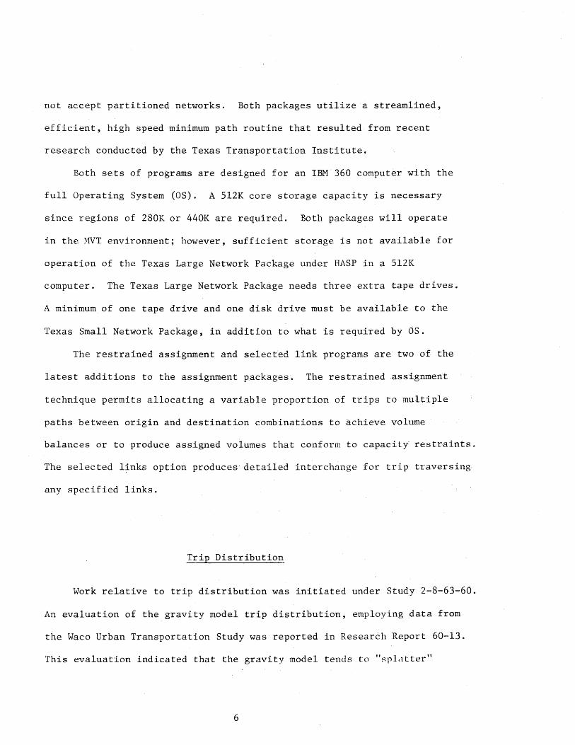
Trip Distribution

Work relative to trip distribution was initiated under Study 2-8-63-60.

An evaluation of the gravity model trip distribution, employing data from

the Waco Urban Transportation Study was reported in Research Report 60-13.

This evaluation indicated that the gravity model tends to "splatter"

6

trips between nearly every possible combination of zone pairs. Such

a travel pattern is not observable in the real world - unless a very

small number of extremely large zones are employed.

Gravity Model Evaluation

The following comparisons were made using the gravity model distri-

bution of the Waco 0-D Survey data:

(1) The trip table resulting from the gravity model distribution of observed trip ends was compared with the observed trip table (zone to zone movements as obtained by the expanded Home Interview Survey).

(2) The gravity model distributed trips were assigned to the existing network (E-2) and the assigned volumes compared with the assignment of the D.U. Survey data.

A single purpose, three purpose, and seven purpose gravity model was

calibrated for internal auto-driver trips. It was concluded that the

three purpose (home base work, home base non-work, and non-home base)

gave somewhat better results than the single purpose; and, that the seven

purpose did not show significant improvement over the three purpose model~

Gravity models were calibrated with and without a ''time barrier'' on

the Brazos River crossings. It was found that a two (2.0) minute time

barrier was appropriate.

Models (single, three, and seven purpose) were calibrated with intrazonal trip ends both included and excluded.

Models were calibrated for the three purpose {HBW, HBNW, NHB) both with and without terminal times.

The following discussion is based on the three purpose model, using

a two minute time barrier, without terminal times, and with the intrazonal

trips being distributed by the model.

7

The number of zone pairs having various levels of trip interchanges

are shown in Table 2. It will be noted that the dwelling unit survey

produced what might be considered to be an unrealistically low estimate

of zone pairs (512) having one to four trip interchanges. Analysis of

the survey data would suggest that about 1,500 to 2,000 zone pairs might

logically fall within this range. This "underestimate" is to be expected

since expansion factors of 4 or less can occur only with a sampling rate

of about 25 percent or higher. Such a small expansion factor will occur

only in sparsely developed zones where the sampling rate is very high.

On the other hand, the gravity model produces an unacceptable high

number of zone pairs with trip interchanges in the one to four stratum.

Further, it yields a totally unrealistically low estimate of the zone

pairs with no trip interchanges.

Further review of the cumulative totals and cumulative percentages

shown in Table 2 suggests that the survey trip table and the gravity

model trip table agree quite well beginning with the 12 to 20 trip

interchange stratum. This, however, is misleading as may be seen from

the data shown in Table 3. This table shows the comparisons of the survey

and the gravity model results for those zone-to-zone movements for

which either the survey data or the gravity model had more than 300

internal auto-driver interchanges. Although some of the comparisons

agree quite well, the bulk of them show that the gravity model is

severely underestimating the larger volume zone interchanges.

Other specialized summary tabulations indicated that there were

84 zone pairs for which the gravity model under or overestimated

8

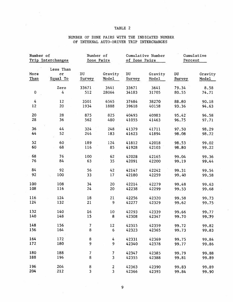
TABLE 2

NUMBER OF ZONE PAIRS WITH THE INDICATED NUMBER OF INTERNAL AUTO-DRIVER TRIP INTERCHANGES

Number of Number of Cumulative Number Cumulative Trip Interchanges Zone Pairs of Zone Pairs Percent

Less Than More or DU Gravity DU Gravity DU Gravity Than Equal To Survey Model Survey Model Survey Model

Zero 33671 3641 33671 3641 79.34 8.58 0 4 512 28064 34183 31705 80.55 74.71

4 12 3501 6565 37684 38270 88.80 90.18 12 20 1934 1888 39618 40158 93.36 94.63

20 28 875 825 40493 40983 95.42 96.58 28 36 562 480 41055 41463 96.75 97.71

36 44 324 248 41379 41711 97.50 98.29 44 52 244 183 41623 41894 98.08 98.72

52 60 189 124 41812 42018 98.53 99.02 60 68 116 85 41928 42103 98.80 99.22

68 76 100 62 42028 42165 99.04 99.36 76 84 63 35 42091 42200 99.19 99~44

84 92 56 42 42147 42242 99.31 99.54 92 100 33 17 42180 42259 99.40 99.58

100 108 ~4 20 42214 42279 99.48 99.63 108 116 24 20 42238 42299 99.53 99.68

116 124 18 21 42256 42320 99.58 99.73 124 132 21 9 42277 42329 99.62 99.75

132 140 16 10 42293 42339 99.66 99.77 140 148 15 8 42308 42347 99.70 99~?9

148 156 7 12 42315 42359 99.72 99.82 156 164 8 6 42323 42365 99.73 99.83

164 172 8 4 42331 42369 99.75 99.84 172 180 9 9 42340 42378 99.77 99.86

180 188 7 7 42347 42385 99.79 99.88 188 196 8 3 42355 42388 99.81 99.89

196 204 8 2 42363 42390 99.83 99.89 204 212 3 3 42366 42393 99.84 99.90

9

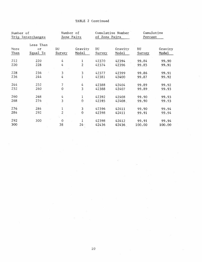
TABLE 2 Continued

Number of Number of Cumulative Number Cumulative Trip Interchanges Zone Pairs of Zone Pairs Percent

Less Than More or DU Gravity DU Gravity DU Gravity Than Equal To Survey Model Survey Model Survey Model

212 220 4 1 42370 42394 99.84 99.90 220 228 4 2 42374 42396 99.85 99.91

228 236 3 3 42377 42399 99.86 99.91 236 244 4 1 42381 42400 99.87 99.92

244 252 7 4 42388 42404 99.89 99.92 252 260 0 3 42388 42407 99.89 99.93

260 268 4 1 42392 42408 99.90 99.93 268 276 3 0 42395 42408_ 99.90 99.93

27·6 284 1 3 42396 42411 99.90 99.94 284 292 2 0 42398 42411 99.91 99.94

292 300 0 1 42398 42412 99.91 99.94 300 38 24 42436 42436 100.00 100.00

10

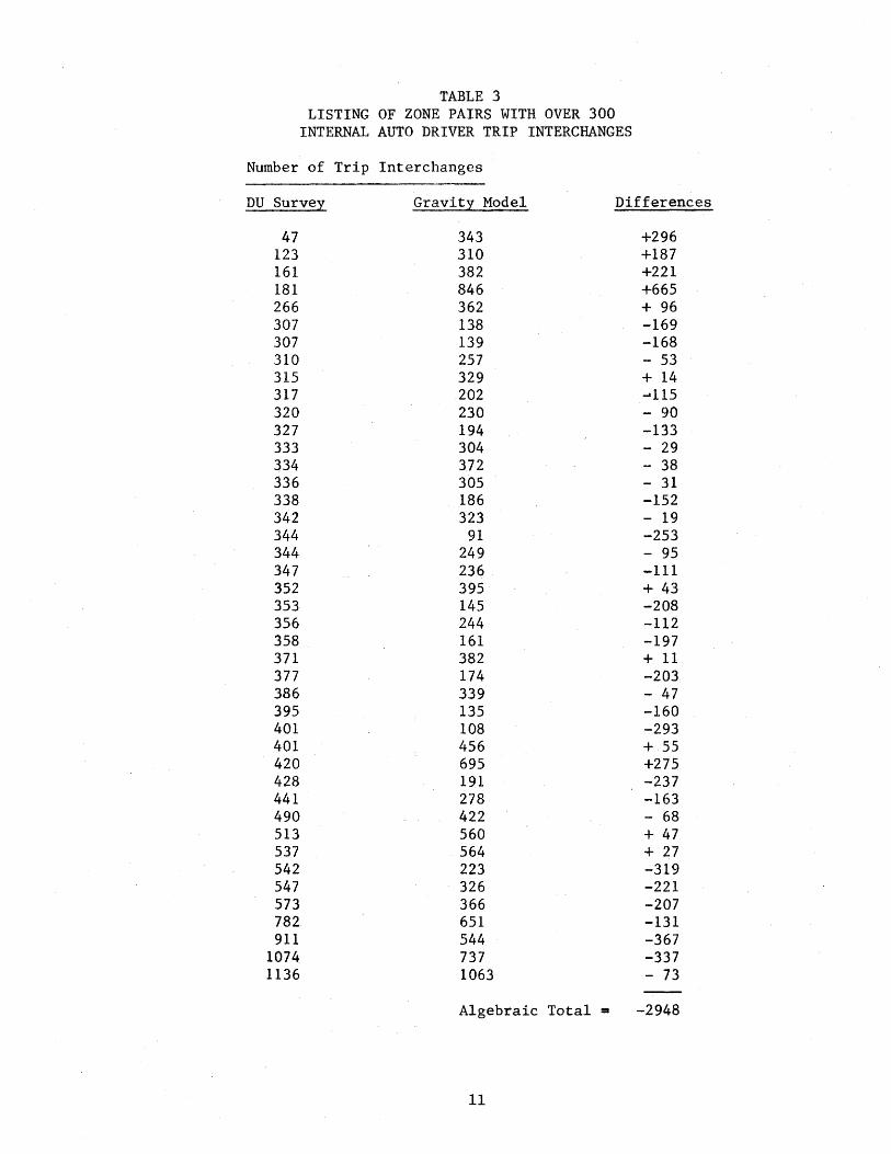
TABLE 3 LISTING OF ZONE PAIRS WITH OVER 300

INTERNAL AUTO DRIVER TRIP INTERCHANGES

Number of Trip Interchanges

DU Survey Gravity Model Differences

47 343 +296 123 310 +187 161 382 +221 181 846 +665 266 362 + 96 307 138 -169 307 139 -168 310 257 - 53 315 329 + 14 317 202 ...al15 320 230 - 90 327 194 -133 333 304 - 29 334 372 - 38 336 305 - 31 338 186 -152 342 323 - 19 344 91 -253 344 249 - 95 347 236 -111 352 395 + 43 353 145 -208 356 244 -112 358 161 -197 371 382 + 11 377 174 -203 386 339 - 47 395 135 -160 401 108 -293 401 456 +55 420 695 +275 428 191 -237 441 278 -163 490 422 - 68 513 560 + 47 537 564 + 27 542 223 -319 547 326 -221 573 366 -207 782 651 -131 911 544 -367

1074 737 -337 1136 1063 - 73

Algebraic Total = -2948

11

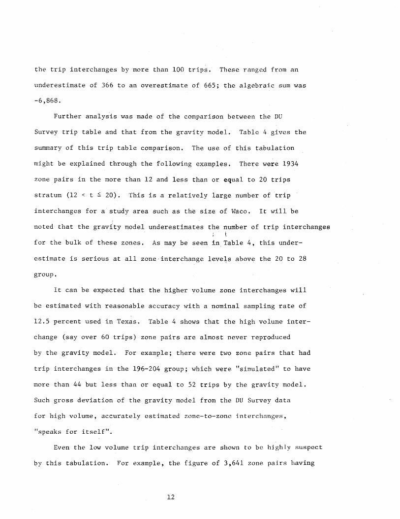
the trip interchanges by more than 100 trips. These ranged from an

underestimate of 366 to an overestimate of 665; the algebraic sum was

-6,868.

Further analysis was made of the comparison between the DU

Survey trip table and that from the gravity model. Table 4 gives the

summary of this trip table comparison. The use of this tabulation

might be explained through the following examples. There were 1934

zone pairs in the more than 12 and less than or equal to 20 trips

stratum (12 < t S 20). This is a relatively large number of trip

interchanges for a study area such as the size of Waco. It will be

noted that the gravity model underestimates the number of trip interchanges (

for the bulk of these zones. As may be seen in Table 4, this under-

estimate is serious at all zone,interchange leve~s above the 20 to 28

group.

It can be expected that the higher volume zone interchanges will

be estimated with reasonable accuracy with a nominal sampling rate of

12.5 percent used in Texas. Table 4 shows that the high volume inter-

change (say over 60 trips) zone pairs are almost never reproduced

by the gravity model. For example; there were two zone pairs that had

trip interchanges in the 196-204 group; which were "simulated" to have

more than 44 but less than or equal to 52 trips by the gravity model.

Such gross deviation of the gravity model from the DU Survey data

for high volume, accurately estimated zone-to-zone interchanges,

"speaks for itself".

Even the low volume trip interchanges are shown to be highly suspect

by this tabulation. For example, the figure of 3,641 zone pairs having

12

!-I w

Table 4

Comparison of Trip Interchanges FromDU Survey and Gravity Model

i ... >

5 Zero 0 < t..:.. 4 12

.. 12 < t .: 20

... .c

~ 20 28 .. 28 < t .: 36 ~ 36 44 !! 44 < t !. 52 .:: 52 60 c. 60 < t !. 68 .... '68 76 ~ 76 < t!. 84 ... 0 84 92

n <t!.1oo

~ 100 108 ... 108 < t ::. 116

j g~ < t.: g; " 132 140 il 140 < t !. 148

~ i~: <t !. i;~ ; ll,4 172 .: 172 < t :. 180 !! 180 ' 188 ;:; 1~8 t .::. 196 -= 196 204 .::: 204 t .::. 212

~ ~;(~ t ~ ;;~

i m :~m. 2bll ~~8 2&8 t ::... ~70 :.76 284 ~84 t .:. 29~ :9: . t . 300

over 300

1-e"o

3617 25i.32

3921 676 185

82 28 11

7 4 4 2 1 0 0 0 0 1 0

TOTAL 3367]

o""<t.';... ~.~, 10

383 li1

27 6 1 2 0 0

51:

~.~r..:.~:... )..l 10

1682 1198 "'366

137 53 22 19

6

3501

:;;umber of Zone Pairs with the Indicated ~umber (t) of Trip Interchanges by DL Su1vey

').()

\.'1.:..t.:...

2 594 722 319 156

75 34 15

6 3 4 1 1 0 1 1 0

!934

' '}.'0 C:. ')b L ~Lit l. ")'!. '}.O.t.'t.,... ...:!!!:_\."' ---2~<-'L,..... -~.:..t....-

2 151 308 193

83 57 33 22 ll

6 4 2 1 0 0 1 1 0 0 0 0 0 0 0 0 0 0 0 0 0

875

0 68

160 119

81 51 24 19 14 10

5 4 3 1 1 0 1 0 1 0 0 0 0 0 0 0 0 0 0 0

562

0 31 84 62 43 35 25 TI 14

6 0

324

0 16 35 39 48 39 14 20 lo

8 5

244

,,'oil ~o<o ,~o <o" o,'l. .._r:§l ,/.._o<o .-..-..'o .. ,-..'!.~> .;;'>'!. <-'':::"o ,_,.<':::"<t. ~1..:..\. _..., bQ'-'t.:,_ ioro._•</;, b'-1(..:,... 'OVtt..'t::... ~.:.~'/ \,.f:J:,'- .,. \.{)ro'-"(,/ '\.),.bi... ,. \.t.l.A.:.t.,.... "\.")"!-'" \..lAC TOTAL

-- -~-~----~- --0 0 0 0 0 0 0 0 0 0 0 0 3641 2 3 1 1 0 0 0 0 0 0 0 0 28064

32 7 9 2 5 1 0 0 0 0 0 0 6%5 32 15 19 7 3 6 1 2 2 0 0 0 1888 35 15 12 8 4 4 2 2 0 2 1 0 825 21 19 13 12 6 1 6 2 3 2 1 0 480 18 13 12 5 6 4 2 1 1 l 0 1 248 16 8 8 7 10 1 1 2 1 3 1 0 183 11 7 3 7 6 2 4 1 1 3 1 2 124 s 7 6 2 5 4 3 3 0 0 2 2 85

5 5 2 1 3 4 2 2 1 2 1 1 62 3 2 3 2 1 1 2 2 0 2 1 1 35 2 5 1 4 1 2 0 2 1 1 3 0 42 l 0 2 0 2 1 2 1 2 1 0 0 17

3 2 2 (J 0 3 0 1 0 0 1 20

89

4 0 0 3 0 0 0 0 1 1 4 20 l 2 0 1 0 1 0 1 0 2 2 21 0 0 0 0 0 2 0 0 0 0 0 9 0 0 0 0 0 0 1 0 1 0 0 10 0 10 0 0 0 21110 8 1 2 1 0 0 0 0 0 0 0 0 12 o o 1 o o o 1 o o o· o 6

116 100

0 010 0 0 0 0 0 4 0 0 0 0 01 l 01 9 0 0110 0 0 0 0 7 0 0 0 0 0 0 010 3 0 0 0 0 0 0 0 0 0 0 010 0 0 0 0 0 0 0 0 0 0 0 0 0 0

0 0 0 0 0 0 0 0 0 0 0 0 0 0 0 0 0 0 0 0

63 56 33 34 24 18 21 16 15

u 3 0 1

24

1-' .p..

Zero 0 < t < 4 -

12 < t c 20 -28 < t < 36 -44 < t .!.

12 20 28 36 44 52

~~<t.!_:~ 68 76 76 < t .!. 84

:~ < t .!. 1~~ ig~ < t .!. i~: 116 124 124 < t .!. 132 132 140 hO < t.!. 148 148 156 156 < t .!. 164

i~~ < t .!. ~~~ 180 188

. 188 < t .!. 196

;~~ c t .!. ~~~ 212 220 220 < t.!. 228 228 236 236 c t .!. 244 244 252 252 < t .!. 260

~:~ c t .!. ;~: 276 28/o 284 c t .!. 292 292 < t < 300

over- 300

Table 4 Continued

•/O t}oo '\. '1.0 '1.'1; ~b \> ... '), L'\.'),0 L'\.".'!1 L'\.">b .......... L'),'>'\. _.,_<oO L'\.fo'!l L'\.'\b L'\.'I:J... • ... ~... _..,o0 00 'I;L'I.~ !oL'I.~ L .. .;:'\ '),L .. .;: f)L._L; 'I;L .. .; <.L .. <JQ \>,L .. <J ....... L .. -' ft'\.f:::tL"--' n'I:JL'<./ ">foL'<./ ...... L'<./ .,,.,-.. ,. bf:::t"'<./ fo'!.'-'<./ '\foL .. / ~-..-"'-' o.'\.L'(./ ..,_f.~ "j ~ 2._ ~ ..,, ~ L ~~., ').0 .2:_ ..:__ ~ 1._ _'l:_ .:;_ ..2:_ .2._ .:!:....._ 1:._ .,_., . .,- TOTAL

o o o--o o o o---o o o o .J o o o o o o--o--o.w:r 0 0 0 0 0 0 0 0 0 0 0 0 0 0 0 0 0 0 0 0 28064 0 0 0 0 0 0 0 0 0 0 0 0 0 0 0 0 0 0 0 0 6565 0 0 0 0 0 0 0 0 0 0 0 0 0 0 0 0 0 0 0 0 1888 0 1 0 0 0 0 0 0 0 0 0 0 0 0 0 0 0 0 0 0 825 0 1 0 0 0 0 0 0 0 0 0 0 0 0 0 0 0 0 0 0 480 0 1 0 0 0 0 0 0 0 0 0 0 1 0 0 0 0 0 0 0 248 1 0 0 0 1 0 2 0 1 0 0 1 0 0 0 0 0 0 0 0 183 0 0 0 3 1 1 1 0 0 1 0 0 0 0 0 1 0 0 0 0 124 1 1 2 1 1 0 0 0 0 1 0 0 0 0 0 0 0 0 0 0 85 1 0 2 0 0 0 2 Q 0 0 0 0 0 0 1 . 0 0 0 0 0 62 0 0 0 0 0 0 0 1 0 0 0 0 1 0 0 0 0 0 0 0 35 3 0 0 0 0 1 0 1 0 0 0 0 0 0 0 0 0 0 0 1 42

. 0 0 0 0 1 0 0 0 0 0 0 0 1 0 0 0 0 0 0 0 17 0 1 0 2 0 0 0 0 0 0 0 0 0 0 0 1 0 0 0 0 20 0 0 1 0 0 0 1 0 0 0 0 0 0 0 0 1 0 0 0 1 20 0 2 0 2 0 0 0 0 0 1 0 l 0 0 0 0 0 0 0 0 2l 0 0 0 0 0 1 0 0 0 0 0 0 0 0 0 0 0 0 0 0 9 0 0 0 1 0 0 0 0 0 0 0 0 0 0 1 0 0 0 0 3 10 0 0 0 0 0 0 0 0 0 0 0 0 0 0 0 0 01 018 1 0 2 0 0 0 0 0 1 0 0 0 0 0 0 0 I} 1 0 0 12

0 0 0 0 01 0 0 0 01 0 0 0 0 0 0 0 01 6 0 0 0 0 0 0 010 01 0 0 01 0 0 0 0 0 4 o o o_Q_ 1 o o o 1 o 1 1 o o o o 1 o o 1 9 0 0 0 0 0 I 0 0 0 I 0 0 0 0 0 0 0 0 0 1 7 0 0 0 0 0 0 0 0 0 0 0 0 0 0 0 0 0 0 0 2 3 o o 1 o o o_Q_ o o o o o o o o o o o o 1 2 o o o o 1 o 1 o ·o o o o o o o o o o o o 3 o o o o o o o o.JL o o o o o o o o o o o 1 0 0 0 0 0 0 0 0 0 _Q_ 0 0 1 0 0 0 0 0 0 1 2 0 0 0 0 0 0 1 0 0 0 0 0 1 0 0 0 0 0 0 1 3 o o o o o o o o o o o_Q_ o o o o o o o 1 1 0 0 0 0 0 1 0 0 0 0 0 0 _Q_ 0 0 0 0 0 0 2 4 0 0 0 0 0 0 0 0 0 0 0 1 1 _Q_ 0 0 0 0 0 1 3 0 0 0 0 0 0 0 0 0 0 0 0 0 0 0 0 0 0 0 01 o o o o o o o o o o o o o o -o__j)_ o o o o o 0 0 0 0 0 0 0 01 0 0 0 0 0 0 0 0 0 0 l 3 0 0 0 0 0 0 0 0 0 0 0 0 0 0 0 0 0 c 0 0 0 0 0 0 0 0 0 0 0 0 0 0 01 0 0 0 0 0 0 01 0 1 0 0 1 0 0 0 0 0 0 0 0 0 l 0 0 0 0 !.2_ 24

38 42436

no trip interchanges by the gravity model is only about eight percent

of the 42,436 total possible zone-to-zone interchanges. Conversely,

38,795 (42,436 minus 3,641) or 92 percent of all zone pairs have one

or more trips by the gravity model. Thus, the gravity model distributed

one or more trips between the vast majority of possible zone pairs.

It seems unrealistic to suppose that anything approaching this dispersion

of travel ever occurs in the real world.

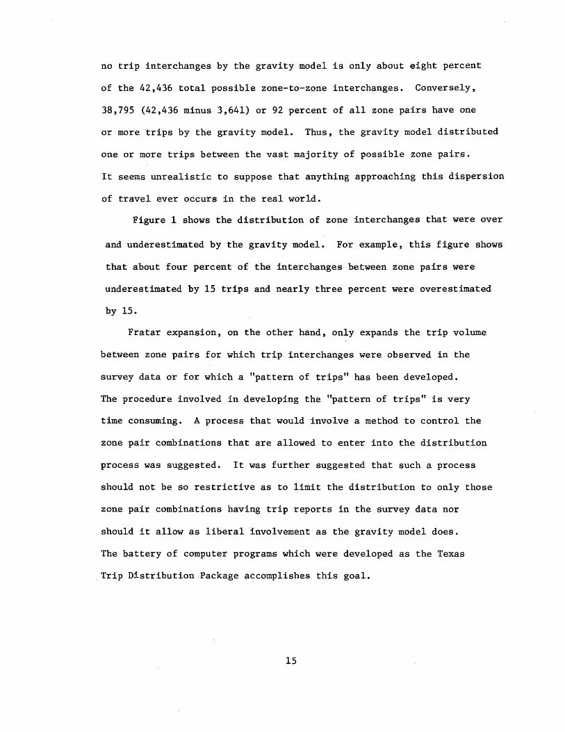
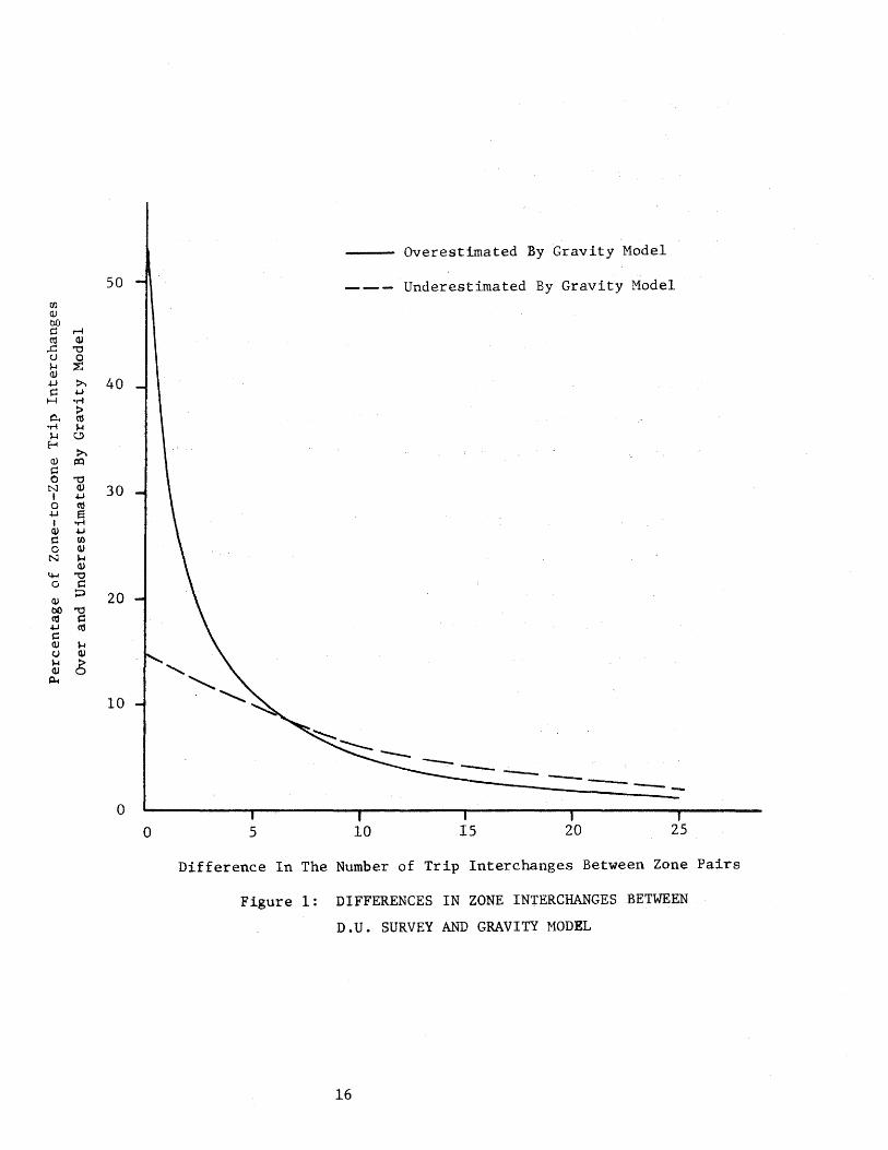
Figure 1 shows the distribution of zone interchanges that were over

and underestimated by the gravity model. For example, this figure shows

that about four percent of the interchanges between zone pairs were

underestimated by 15 trips and nearly three percent were overestimated

by 15.

Fratar expansion, on the other hand, only expands the trip volume

between zone pairs for which trip interchanges were observed in the

survey data or for which a "pattern of trips" has been developed.

The procedure involved in developing the "pattern of trips" is very

time consuming. A process that would involve a method to control the

zone pair combinations that are allowed to enter into the distribution

process was suggested. It was further suggested that such a process

should not be so restrictive as to limit the distribution to only those

zone pair combinations having trip reports in the survey data nor

should it allow as liberal "involvement as the gravity model does.

The battery of computer programs which were developed as the Texas

_Trip Distribution Package accomplishes this goal.

15

rn Q) bJ)

~ ...-l ro QJ

...c: "'0 (.) 0 H ~ QJ ~ >. ~ 4..J

H •rl

~ :> (13

•rl ""' H c.!>

H >.

Q) j:Q ~ 0 "'0 N QJ I 4..J 0 ro ~ !l I Q) ~

r:: tll 0 Q)

N ""' C1J

\.j..j "'0 0 r::

0 (1)

bO "'0 ro r:: ~ (13 r:: QJ

""' (.) Q) .... 6 Q) ~

50

40

30

20

10

0

0

Overestimated By Gravity Model

--- Underestimated By Gravity Model

-----5 10 IS 20 25

Difference In The Number of Trip Interchanges Between Zone Pairs

Figure 1: DIFFERENCES IN ZONE INTERCHANGES BETWEEN

D.U. SURVEY AND GRAVITY MODEL

16

Texas Trip Distribution Package

The Texas Trip Distribution Package is a collection of computer

programs having considerable flexibility in performing trip distributions.

The methods range from directionally expanding existing trip matrices

to new totals, to performing synthetic distributions using a constrained

interactance model.

The basic interactance model applies trip lengths directly in the

distribution process and, consequently, needs no calibration. Other

properties of the interactance model are similar to a gravity model

without 'F-factors'. By applying a constraint, derived from a

concept related to intervening opportunities and supported by analysis

of interchange propensity, only selected zone pairs enter into the dis­

tribution rather than all possible zone pair combinations as with the

gravity model. This limit function is the essential element that differ­

entiates the Texas trip distribution procedure from the conventional

gravity models in concept.

A sector structure may be imposed to.permit a statistical analysis

for, and correction of, sector interchange bias created by socio­

economic-topographical travel barriers·. Movements having external

terminals may be processed simultaneously with the synthetic distribution

of internal trips.

The Texas Trip Distribution Package is designed to interface with

the Texas Small and Large Network Traffic Assignment Packages. It

has been prepared for an IBM 360 computer system, but is programmed

almost entirely in FORTRAN (except for an entry into the system sorting

17

program) and, therefore, is not highly machine dependent. The coding

in the programs has been optimized for processing efficiency in order

to· minimize execution time. For benefit of the user, simplicity and ease

of operation have been emphasized rather than superflexibility due

to its accompanying operational complexities. However, a feature has

been provided to permit the exercising of options to satisfy abnormal

flexibility needs.

The package is capable of accommodating trip tables having up to 4800

zones using a computer with 512,000 bytes of core storage available.

By making a simple change, the capacity can be varied to conform to any

partition or region size in excess of about 110,000 bytes.

Completion of this research activity was carried over on Study

2-10-71-167 which is the sequel to Study 2-10-68-119. Operating

instructions for the Texas Trip Distribution Package was published as

Research Report 167-1; internal documentation will be reported in

Research Report 167-2.

Other Computer Programming

Adoption of the IBM 360 computer by both the Texas Highway Depart­

ment and Texas A&M University, of course, required that the computer

programs used in Urban Transportation Planning be rewritten. In addition

to the substantial programming effort required to develop a small and

large traffic assignment packages, an unusually large programming

18

effort was required to maintain operational capability. This unusually

large required programming effort was due to the fact that numerous

versions of the IBM 360 Operating System were adopted during the course

of study no. 2-10-68-119. These changes of the Operating System fre-

quently required the complete reprogramming of the small and large

traffic assignment packages. The changes in the operating system caused

an even greater repeat of programming effort for the Trip Distribution

Package since this package was in the development stage. It is

estimated that over two man years was expended in regaining operational

capability on the three program packages.

Accuracy of Employment and Non-Home Trip Ends from Home Interviews

Comparisons were made of employment as estimated from the home

interview survey data with the reported employment obtained by field

listing (interview) of each employer in the study area. A comparison

was also made for non-home trip ends for six selected zones in the McAllen-

Pharr Urban Transportation Study area where manual cordon counts were made.

Study Area

The McAllen-Pharr Urban Transportation Study was conducted by the

Texas Highway Department in 1968. The study area was roughly rectangular

with sides six and twelve miles in length and included the towns of

Mission, McAllen, and Pharr. The total population of the study area

was estimated at 79,400; of these, 70,800 persons were over five years of

19

age. In addition, there are an estimated 300,000 persons living in

the surrounding area including the city of Reynosa, Mexico.

Data Collection

The data involved in this report were collected by the Planning

Survey Division of the Texas Highway Department during the data collection

phase of the McAllen-Pharr Urban Transportation Study. The number

of employees who worked in a particular zone was determined by contacting

each employer within the study area. These employers were asked for the

total number of persons he employed full-time (three or more days per

week) and part time at that particular work site. These employment

data were collected at an average cost of 0.31 man hours per employer.

No information was obtained on domestic employees.

The total number of vehicles which entered each of the six

zones was obtained by manual cordon counts. These counts were made by

hourly periods beginning before the morning peaks and continuing until

the traffic had subsided that evening. The six survey zones were chosen

because there were no dwelling units in these zones and the internal

street pattern prohibited through trips.

Data Compatibility

Table 5 lists the employment data totals for the study area as

tabulated from the data tape and before any adjustments for absenteeism

were made to the Type 2 and Type 3 card data.

In order to use the external data as a guide to the number of

employees who cross the study area cordon, some adjustment must be

made for the absentee rate. If it is assumed that this rate is the same

20

TABLE 5

EMPLOYMENT TOTALS BEFORE ADJUSTING TYPE 2 AND 3 CARD DATA FOR ABSENTEEISM

(all survey data expanded to population)

Source Number of Employees

Employer Survey

Dwelling Unit Survey:

Employment Raport (Type 6 card):

Total Employed Labor Force

Total Labor Force, worked on previous day

Internally Employed Labor Force

Internally Employed Labor Force, worked on previous day

Trip Report (Type 2 card):

First Work Trip

External Data (Type 3 card) :

a) Live out of area Entering to work 3,736

Leaving from work 3,520

b) Live in area Entering from work 4,128

Leaving to work 3,979

21

Avg.

Avg.

16,910

20,415

17,334

16,963

14,616

17,475

3,628

4,054

for employed persons residing outside the study area as it is for those

employees residing inside the study area, the information on the Type

6 cards, Employment Report, may be used as a basis for estimating

absentees for the Type 3, External Survey cards.

The number of employees in the total employed labor force (that

is, those persons who live within the study area and are employed)

is 20,415 persons. Of this 20,415 persons, only 17,334 reported having

gone to work on the interview day. This indicates an absentee rate of

14.7 percent; calculated as follows:

20,415 - 17,334 --~--2-0-,~4-1-5~-- x 100 = 14.7 percent absent.

The number of persons working within the area and living outside was

extracted from the Type 3, External Survey cards. It was necessary to

assume that the trip purpose of all passengers was the same as that of

the driver. Any adverse affect of this assumption should be minimal

since the occupancy of vehicles entering the area to work was only 1.4

persons.

The employment from the Type 3 cards was obtained by multiplying

the expansion factor (24-Hour Factors) by the number of persons in the

car for each Type 3 card with one trip end "home" or "serve passenger" and

the other "work" and summing the resulting product for each zone of

employment. For purpose of a check, the data were tabulated as sub-totals

by zones of employment for persons entering the area to work, leaving

the area from work; and leaving the area to work and entering the area from

work. No significant difference was found in the inbound and the outbound

22

volumes.* Consequently, the average was used in the analysis. It

was necessary to assume that all persons who left the area from work

within the area lived outside the area. Because of the rigid grid street

arrangement, this appears to be a reasonable assumption.

Estimation of Internal Employment

Three different approaches were taken in order to obtain an estimate

of the number of persons employed within the study area. These methods were:

method 1: estimate from total employed labor force: The total employed

labor force obtained in the home interview survey includes all persons

who claim to be employed regardless of place of employment. Therefore

adjustments must be made for persons who live in the area and work

outside as well as those who live outside of the area and work within

the area. The calculations involved in this adjustment are as follows:

Total Employed L~bor Force (from Type 6 card)

Entering area to work (from Type 3 card) = +3,628

Adjusted for absentees = 3,628 100 - 0.147

Leaving area to work (from Type 3 card) = -4,054

Adjusted for absentees = -4,054 1.00 - 0.147

Estimated Internal Employment

20,415

+ 4,241

- 4,759

19,897

method 2: estimate from internally employed labor force: The internally

employed labor force data as determined from the Type 6 card, Employ-

ment Report, reflect ~he numbe~ of employees who live and work within the

study area. Therefore, in order to establish a total which could be

*A'sign test was conducted on the inbound employees as listed by zone of employment. From this test it was concluded that there is no statistical difference in the average inbound or outbound trips. How­ever, the reader might notice that the totals are lower for trips from work. This is to be expected due to after work shopping trips.

23

compared to the employer survey, the number of_ employees entering the

area to work was added to the number of persons employed in each zone

as obtained from the internally employed labor force data.

Internally Employed Labor Force (Type 6 card) 16,963

Entering Area to Work (Type 3 card) +3,628

3,628 Adjusted for absentees = ------~--~ 1.00 - 0.147 + 4,241

Estimated Internal Employment 21,204

method 3: estimate from first work trip·: The first work trip data provide

an estimate of the total of the employees who went to work on an average

day regardless of the location of their employment. In order to get an

estimate of the total employment from this, the number of persons who enter

the area to work must be added and the number persons who leave must

be subtracted. The total, factored for absentee persons, becomes:

First Work Trip (Type 2 card) 17,476

Entering Area to Work + 3,628

Leaving Area to Work - 4,054

17,050

Estimated Internal Employmen~ Adjusted for Absentees

17,050 1.00- 0.147 = 19 ' 988

Comparisons of Estimates: It should be noted that in the "estimate

from the total employed labor force" and in the "estimate from the first

work trip", the external survey data are used to estimate both the number

24

of persons leaving and entering the area to work. In the "estimate by

the internally employed labor force", the number of persons leaving the

area to work is estimated by the dwelling unit survey.

The final estimates of internal employment differ by about 1300

employees, with the estimates from the total employed labor force and

the first work trip about the same and the estimate from the internally

employed labor force higher. After considering the possible sources

of error in data collection as well as the assumptions in each of the

estimates, it is concluded that method 2 is potentially the most

reliable. Therefore, the estimate from the internally employed labor

force was considered the best estimate of the employment in the McAllen­

Pharr Study; this estimate was 21,200 employees.

The employment found from the employer survey was 16,910 employees.

The obvious discrepancy of nearly 4,300 more employees is probably due

to several sources. The major portion of this difference is believed

to be the domestic personnel not reported in the employer survey and

for which no estimate is possible. Other sources which might contribute

to the difference are persons who claim to be employed, but who, in

truth, are not employed; employers who do not report all of their

employees because some are Mexican nationals working illegally; and

problems of obtaining detailed information, without misunderstanding,

in any external survey.

comparison of employment estimates by smaller geographical areas

Comparisons of employment estimates were performed by zones, districts,

and census tracts. As a basis of comparison, the employer survey was

25

assumed as the standard to which the zone by zone data based on the

internally employed labor force are compared. Again, one should realize

that the employer survey does not include domestic help. Consequently,

if there was any domestic employment in a particular zone, the employer

survey would underestimate the employment for that zone. Further, the

employment estimate from the home interview should be expected to exceed

that from the field listing of employment (employer survey) since the

total estimates of the employment from the 0-D Survey are greater t~an

the employment from the employer data. In no case should the employment

estimate from the home interview be expected to be less than that obtained

by the employer survey.

Similar adjustments were made to the data by zones, districts, and

census tracts, as were made to the totals in the preceding section.

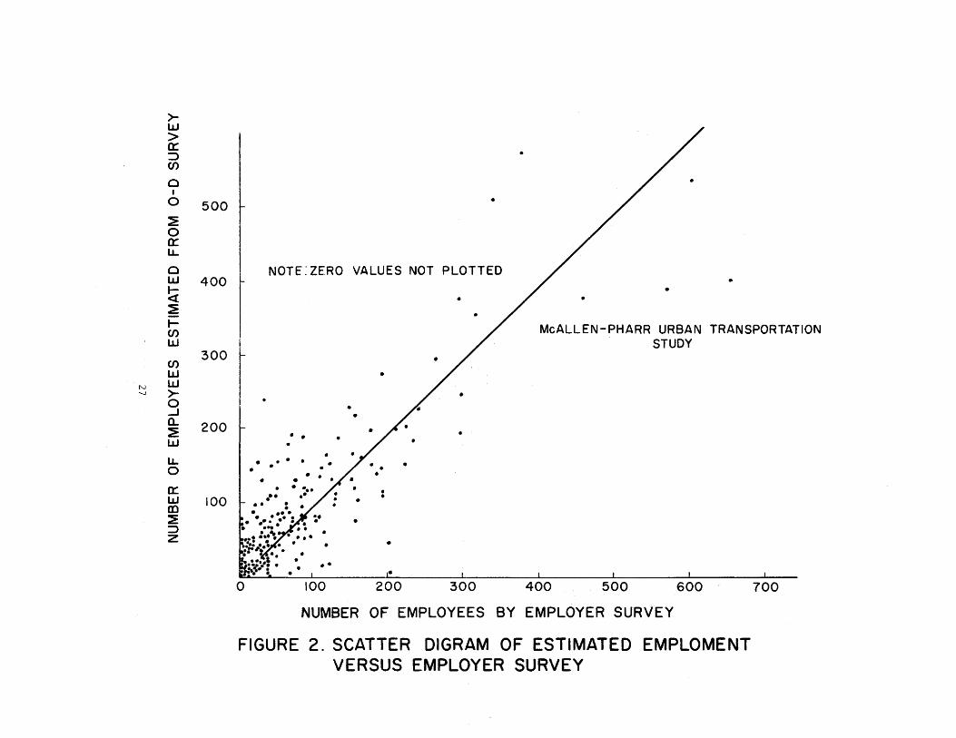
serial zones: There are 363 serial zones in the McAllen-Pharr study area;

a scatter diagram of the data is shown in Figure 2. This plot indicates

substantial variation between the 0-D Survey data and the employer

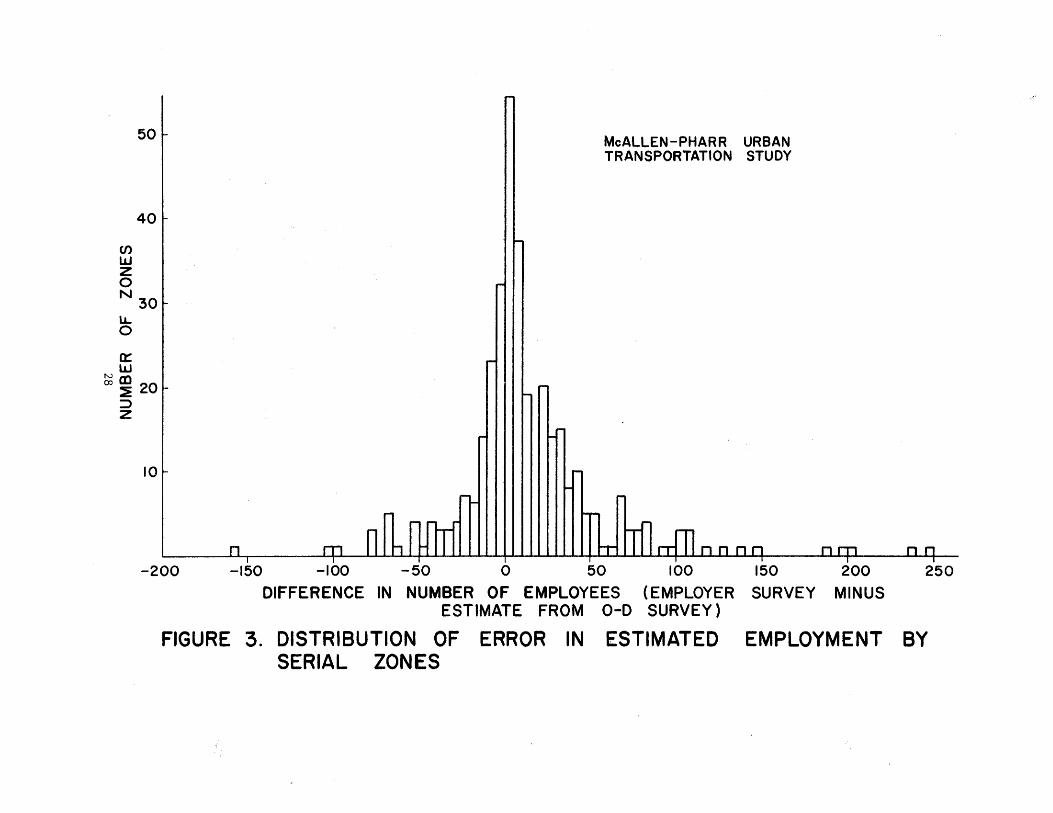
survey data. The distribution of error (employer survey minus 0-D

Survey) is shown in Figure 3. Zones which had zero employment from

both the 0-D Survey and the employer survey are not shown in this graph.

As discussed above, these differences are expected to be zero or positive

but not negative. However, Figure 3 shows that a number of zones (113)

which are estimated to have fewer employees by the 0-D Survey data than

by the Employer Survey. This raises a question as to the reliability of using

.home interview data to estimate activities of the non-home end.

Figure 4 shows the distribution of the number of zones with a

given percent error for different zone size groups. This figure indicates

26

>-UJ > a:: :::) (J)

0 I

0

:E 0 a:: LL

0 UJ

~ :E .,_ (J) UJ

(J) UJ

N w -....! >-

0 ...J a.. :E w LL 0

a:: w CD :E :::) z

500

400 I 300 ~

200

100

0

•

•

NOTE:ZERO VALUES NOT PLOTTED

• • . • • • •

•

.. 100

• •

•

•

• •

•

• 200

•

•

•

300

•

McALLEN-PHARR URBAN TRANSPORTATION STUDY

400 500 600 700

NUMBER OF EMPLOYEES BY EMPLOYER SURVEY

FIGURE 2. SCATTER DIGRAM OF ESTIMATED EMPLOMENT VERSUS EMPLOYER SURVEY

(/) w z 0

50

40

N 30 LL 0

a:: w

~ ~ 20 => z

10

McALLEN-PHARR URBAN TRANSPORTATION STUDY

-200 -150 -100 -50 0 50 100 150 200 250

DIFFERENCE IN NUMBER OF EMPLOYEES (EMPLOYER SURVEY MINUS ESTIMATE FROM 0-D SURVEY)

FIGURE 3. DISTRIBUTION OF ERROR IN ESTIMATED EMPLOYMENT BY SERIAL ZONES

N \0

CJ)

l.&J 10 t­z 0 N LL 0 ~ l.&J 5 1-m ~ :;:)

z

(/)

l.&J z 010 N LL. 0

~ w m 5 ~ :::> z

r-T'"

,...... ~

ZONES WITH 0-10

EMPLOYEES

r""T"1 r""'T""

I'"'T""' I I ...,...

rn I ffirllll [II rn I""'T""

r I

-100 0 100 200 300 400 500

PERCENT ERROR EMPLOYEE DATA

ZONES WITH 10-50

EMPLOYEES

n_ -

-100 0 100 200 300 400 500

PERCENT ERROR EMPLOYEE DATA

FIGURE 4

CJ)

w z 10 0 N

LL. 0

ffi 5 m :E :::> z

ZONES WITH 50-100

EMPLOYEES

-100 0 100 200

PERCENT ERROR EMPLOYEE DATA

CJ)

w z

ZONES WITH. MORE THAN

100 EMPLOYEE s 0 10 N

LL. 0

~ w m 5 ::e :::> z

-100 0 100 200

PERCENT ERROR EMPLOYEE DATA

that the 0-D Survey data tend to underestimate the employment in

serial zones, regardless of zone size. More significantly, the employment

estimates from the 0-D Survey data have a high percentage error even

in the larger zones (over 100 employees).

It is concluded that acceptable estimates of employment by serial

zones are not provided by the 0-D Survey for the .size zone used in the

McAllen-Pharr Urban Transportation Study.

districts: An analysis similar to that for serial zones was also made

for districts and census tracts in order to evaluate the effect of larger

aggregations. Figures 5 through 7 present a summary of the employment

comparisons by the 102 districts.

As expected, the 0-D Survey does a better job of estimating employment

at district level than it does at the serial zone level. However, it is

concluded that the 0-D Survey data do not yield acceptable estimates of

employment for districts of the size used in the McAllen-Pharr Study.

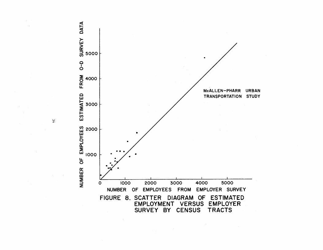
census tracts: Results of the comparison of estimated employment and

that obtained from the employer survey for the 20 census tracts which

are partially or wholly within the study area are given in Figures 8

through 9.

It is concluded that the origin-destination survey does not yield

an acceptable estimate of the employment by zones, districts, or census

tracts.

30

>-LI.J > a: ~ C/)

0 I

0

~ 0 a: lL

0 LLJ

!i ~ t-C/) IJ.J

C/) w ....... IJ.J

IJ.J >-0 ....J (l.

:E w lL 0 a: IJ.J m :E :::> z

2000

1500

1000

900

800

700

600

500

400

300

·/ /

/.

/ /

NOTE: ZEROS NOT PLOTTED /

:. / . . . . .. . . 7 •

/

/ /

/ / -McALLEN-PHARR URBAN TRANSPORTATION

• STUDY

~­/

. /• 200 1- • • •••• , • . : . . .. . . / .. . . :: . . . 100 1:-,. J ~ • ... /•· .

•• • • • • ••••

NUMBER OF EMPLOYEES BY EMPLOYER SURVEY

FIGURE 5. SCATTER DIAGRAM OF ESTIMATED EMPLOYMENT VERSUS EMPLOYER SURVEY BY DISTRICTS

20

en .... u 0:: ..... en cs LL. 10 0

v.> a:: N LLI

m ~ ::::> z

1-

1-

I""'-

McALLEN-PHARR URBAN

TRANSPORTATION STUDY

11--o

r--

1--

1--

r--

I--

...-t-- nn r--1 ,.-, 1"1

I I I I

-300 -200 -100 0 100 200 300

DIFFERENCE IN NUMBER OF EMPLOYEES (EMPLOYER SURVEY MINUS ESTIMATE FROM 0-D SURVEY)

FIGURE 6. DISTRIBUTION OF ERROR IN ESTIMATED EMPLOYMENT BY DISTRICTS

(J)

I­(._)

0:: 1-(f)

0

l1.. 0

a::: L&.J m ~ ~ z

(f)

I-u a:: 1-(f)

0

l1.. 0

a::: w m ~ ::> z

I 0 ,_

5 .._

-100 0

.--

20 -

15 r-

~

10 i-

~

--5 1-

.--

1--r--

DISTRICTS WITH FEWER THAN 100 EMPLOYEES

100 200 300

PERCENT ERROR

DISTRICTS MORE EMP

WITH 100 OR LOYEES

McALLEN- PHA RR URBAN

ON STUDY TRANSPORTATI

.--

I

I

400

-100 0 100 200

PERCENT ERROR

FIGURE 7. DISTRIBUTION OF PERCENT ERROR FOR DISTRICTS

33

~ c

>-LLJ > a:: ~ 5000

c I

0

~ 4000 a:: LL

0 LLJ

~ 3000 ::E ~ CJ)

w LLJ ~

~ 2000 LLJ >-9 a.. ::E LLJ 1000 LL 0

0::: LLJ m ::E ::> z 0

•

•

•

McALLEN-PHARR URBAN TRANSPORTATION STUDY

1000 2000 3000 4000 5000

NUMBER OF EMPLOYEES FROM EMPLOYER SURVEY

FIGURE 8. SCATTER DIAGRAM OF ESTIMATED EMPLOYMENT VERSUS EMPLOYER SURVEY BY CENSUS TRACTS

CJ) ..._ (.) <( a: ..._

CJ)

::l CJ)

z w (.)

w lL V1 0 a: w m :E ::l z

4r McALLEN-PHARR URBAN

TRANSPORTATION STUDY I I I I

31-

2t-

II-

I

-300-200 -100 0 100 200 300 400 500 600 700 800

DIFFERENCE IN NUMBER OF EMPLOYEES (EMPLOYER SURVEY MINUS ESTIMATE FROM 0-D SURVEY)

FIGURE 9. DISTRIBUTION OF ERROR IN ESTIMATED EMPLOYMENT BY CENSUS TRACTS

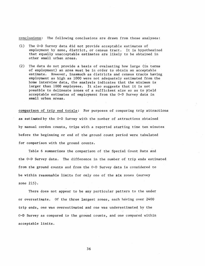
conclusions: The following conclusions are drawn from these analyses:

(1) The 0-D Survey data did not provide acceptable estimates of employment by zone, district, or census tract. It is hypothesized that equally unacceptable estimates are likely to be obtained in other small urban areas.

(2) The data do not provide a basis of evaluating how large (in terms of employment) an area must be in order to obtain an acceptable estimate. However, inasmuch as districts and census tracts having employment as high as 1000 were not adequately estimated from the home interview data, the analysis indicates that the minimum is larger than 1000 employees. It also suggests that it is not possible to delineate zones of a sufficient size so as to yield acceptable estimates of employment from the 0-D Survey data in small urban areas.

comparison of trip end totals: For purposes of comparing trip attractions

as estimatedby the 0-D Survey with the number of attractions obtained

by manual cordon counts, trips with a reported starting time ten minutes

before the beginning or end of the ground count period were tabu~ated

for comparison with the ground counts.

Table 6 summarizes the comparison of the Special Count Data and

the 0-D Survey data. The difference in the number of trip ends estimated

from the ground counts and from the 0-D Survey data is considered to

be within reasonable limits for only one of the six zones (survey

zone 215).

There does not appear to be any particular pattern to the under

or overestimate. Of the three largest zones, each having over 2400

trip ends, one was overestimated and one was underestimated by the

0-D Survey as compared to the ground counts, and one compared within

acceptable limits.

36

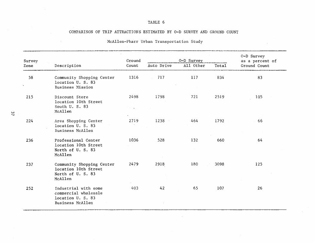
TABLE 6

COMPARISON OF TRIP ATTRACTIONS ESTIMATED BY 0-D SURVEY AND GROUND COUNT

McAllen-Pharr Urban Transportation Study

0-D Survey Survey Ground 0-D Survey as a percent of Zone Description Count Auto Drive All Other Total Ground Count

58 Community Shopping Center 1316 717 117 834 83 location U. S. 83 Business Mission

215 Discount Store 2498 1798 721 2519 105 location lOth Street South U. s. 83

w McAllen -.....1

224 Area Shopping Center 2719 1238 464 1792 66 location U. S. 83 Business McAllen

236 Pr.ofessional Center 1036 528 132 660 64 location lOth Street North of U. S. 83 McAllen

237 Community Shopping Center 2479 2918 180 3098 125 location lOth Street North of U. S. 83 McAllen

252 Industrial with some 403 42 65 107 26 commercial wholesale location U. S. 83 Business McAllen

Although a small number of zones were included in this study, it is

believed that the data are sufficient to indicate that trip attractions

are not estimated with an acceptable degree of accuracy by the 0-D

Survey for the size of zone that must be used in small urban areas.

The Accuracy of All-Or-Nothing Assignments In Estimating Turn Movements

The accuracy of the traffic volume estimates resulting from traffic

assignments has been considered sufficient for system planning purposes.

However designers, confronted with a need for design data, have also

employed these results. As turning movements are furnished as a routine

portion of traffic assignment output, these results have been considered

a logical source of turning volume estimates for proposed transportation

facilities. The adequacy of assigned turning volumes is cause for concern

if these estimates are to be employed in design.

A preliminary analysis of turn movements was performed as a

satellite to the study on the effect of network detail on the all-or-

nothing traffic assignment using information from the Waco Urban

Transportation Study.

Comprehensive ·turning movement count data for the express purpose

of detailed analysis of turn movements was not collected during the

origin-destination .survey. Hence, there were only 25 intersections,

scattered throughout the study area which could be included in the

38

analysis using all three coded networks. These three networks were:

• The operational (E-2) network having 410 nodes.

• An intermediate density network with 1930 nodes.

• A detailed network with 5629 nodes.

The following count data were available for the 25 intersections.

(1) A.M. peak period count.

(2) P.M. peak period count.

(3) One hour off-peak count, usually 10-11 A.M.

Twenty-four turn movement counts, however, were not available

for the same 25 intersections for which there were counts for peak and

off-peak periods. Thus, the short period counts had to be expanded to

twenty-four hour estimates for comparison with the twenty-four traffic

assignment results.

This was accomplished by adding the two peak period counts to

sixteen times the off-peak hour count on the assumption that turns,

in percent of approach volume, remains constant throughout the day. The

expansion factor of sixteen was selected based on an analysis of volumes

of all roadway sections in the study area with both peak period, off-

peak period and twenty-four hour counts.

An expansion factor was calculated for each of these roadway

sections on the following basis:

24 Hr. Count - (A.M. + P.M. Peak Period Counts) Off Peak Hour Count

The average value of the expansion factor was found to be approximately

sixteen.

39

In order to obtain twenty-four hour turn volume estimates, the

expansion factor was used in the following manner:

Estimated 24 hour volume (Expansion Factor) (Off Peak Hour Count) + (A.M. + P.M. Peak Period Count)

The expanded counts were compared with the turning movements

obtained from the assignment of the observed 0-D trip matrix to the

three coded networks. The assignments were made without turn penalties.

The assigned values were first to be consistently below the estimated

twenty-four hour volumes for all three degrees of network detail.

In an attempt to minimize any influence of the off-peak period

expansion factor, the percent turning movements were compared.

This was done because the percent turns are not as drastically affected

by errors in estimating the expansion factor as are the actual number

of turns.

Left turns, as a percent of approach volume, obtained from expanded

peak period counts were plotted against assigned left turn volumes as

a percent of total assigned approach volume for the 25 intersections

for which there were turn movement counts available. This analysis

suggested that the percentage of turns obtained through an ali-or­

nothing traffic assignment are approximately randomly distributed.

In an attempt to provide a comparative evaluation of the accuracy

of turning assignment for different degree of network detail an accu­

mulated frequency distribution of each of the three networks was prepared.

40

This was done by plotting the accumulated percent of approaches,

for which there were data available, against the difference in percent

between assigned and counted volumes. Percent differences were accumulated

in the direction from large toward smaller algebraic values (i.e.

any negative value is considered smaller than zero; the smallest differ-

ence was thus -100 percent for a turn movement with zero assigned volume).

Only approaches where counts for through or individual turn movements ,f

exceeded 500 vpd. were included in the analysis.

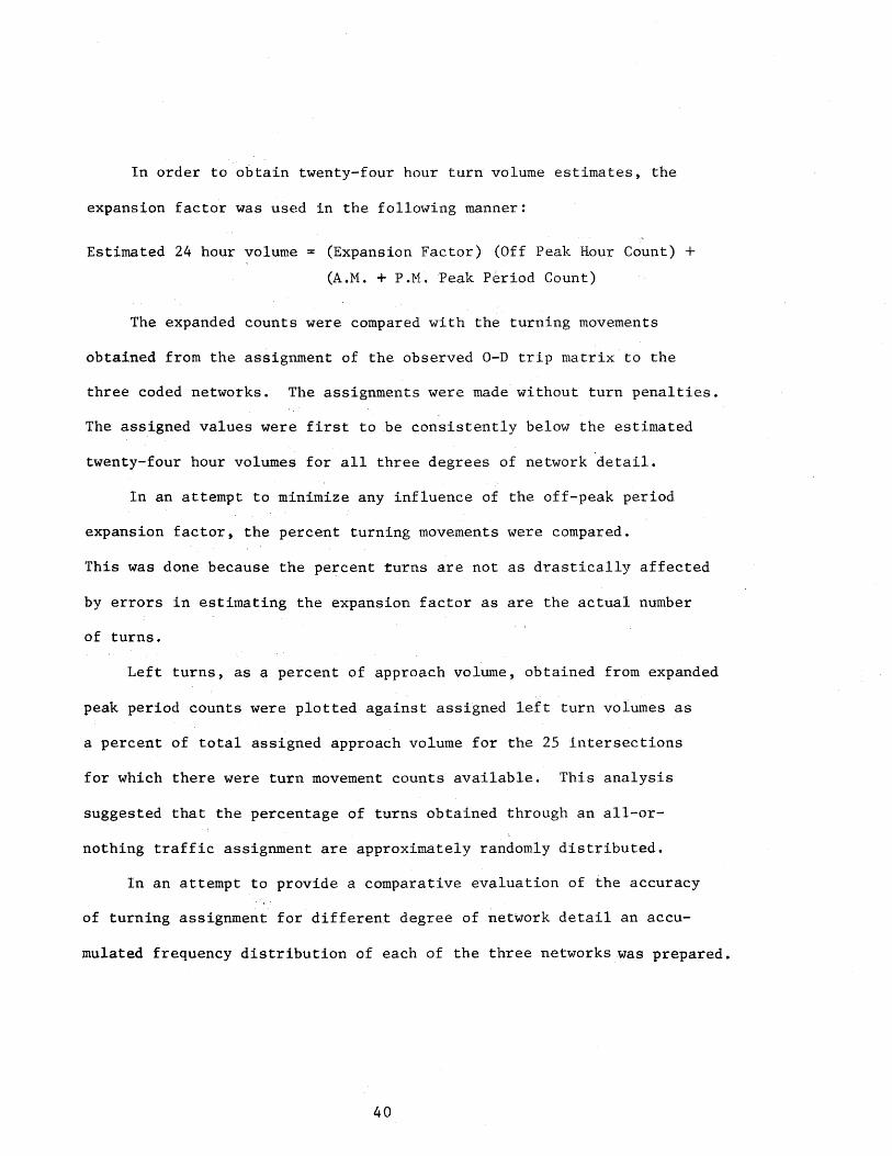
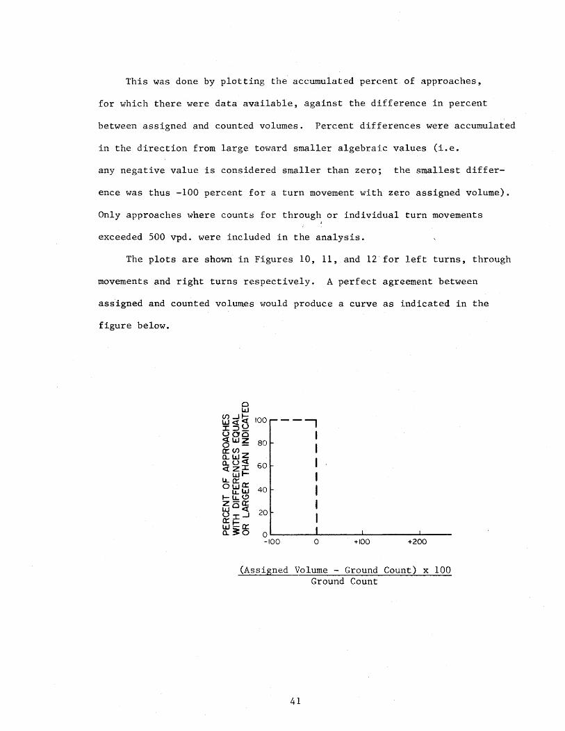
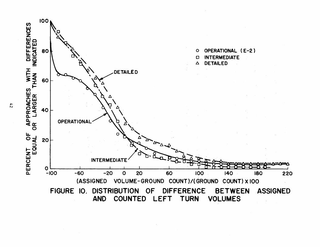
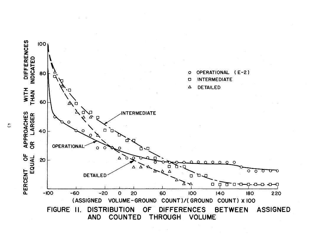
The plots are shown in Figures 10, 11, and 12 for left turns, through

movements and right turns respectively. A perfect agreement between

assigned and counted volumes would produce a curve as indicated in the

figure below.

0 w (J)...Jti 100 ----, w~u :I:::>_

I uoo ~w~ 80

I Q:(J)z a..w<t I a..u:J: 60 <(~t- I LLO::O:: o~w 40 I ..... LL.(!) z-a:: I wo<t U:x:::...J 20 I ffit:a:: a. !to 0

-100 0 +100 +200

(Assigned Volume - Ground Count) x 100 Ground Count

41

U}

~ z We Q:IJJ IJJ LL~ ~(.) co z :I: t:z ~<[

:I: (1)1-LIJ :J:O::

+="-uLaJ

N <[(!) oa:: a::<[ a.....J a.. <[a::

0 LL o-' <[

::> 1-0 zw IJJ (.) £t: LIJ 0..

100

,o

' 801- -~

~-

o OPERATIONAL ( E -2 ) o INTERMEDIATE A DETAILED

·~~" /DETAILED

t~ \ \

~\ \ fl.

~ \~ ,. ~ 0~ ' fl.~

~I::J.~

60

40

OPERATIONAL

20

I . /o'b~ INTERMEDIATE ~!f-Ia:t:s . _ _ _

0 I I I I . · -~:8:~ -100 -60 -20 0 20 60 100 140 180 220

(ASSIGNED VOLUME-GROUND COUNT)/( GROUND COUNT) X 100

FIGURE 10. DISTRIBUTION OF DIFFERENCE BETWEEN ASSIGNED AND COUNTED LEFT TURN VOLUMES

~ w

C/) 100 liJ

0 z L&Jo B::w IJJ~ LL 0 80 lL_ -a 0~

:I:z !::c:~: ~:I: 60 .....

U'Ja::: L&JLLI ::J:(!) Oa::: <( <( 40 o_, Q: 0.. O..o:: <to

lL. _, 20 0<(

:::> .... s z LLI 0 0::

\ \ 0\ ~-o '" ~\D

~ ~ D /INTERMEDIATE

0 ~L\'V o' o 'o 0~ ~

o OPERATIONAL ( E-2)

o INTERMEDIATE

a DETAILED

~ &"' OPERA TIONA~ o ~o ~ ,o

7'~,

~~ o Cl'CL . ~A .~

DETAILED ~- o '0--Q.._ A'- -f5t. "'-6 0 OCr 0 -Q--{J- -0-0- -o--o

LIJ a.. -100 -60 -20 0 20 60 100 140 180 220

(ASSIGNED VOLUME-GROUND COUNT)/( GROUND COUNT) X 100

FIGURE II. DISTRIBUTION OF . DIFFERENCES BETWEEN ASSIGNED AND COUNTED THROUGH VOLUME

~ ~

en w oo Zw UJI-Cl:c:r:

100 ~ ,,

6 0~,

w LL ~ 80 LLO D'~' ~~ o OPERATIONAL ( E -2)

-z 0-

:I:Z 1-C -::r:: ~ ..... 60

en a: UJIJJ

' :I: (!) oa:: <(C( 0'...J 40 a:: a.. a: ~0

' 0 ~~

\ \ 0

\ b .

, \~DETAILED .

~ 6~ ........._~0 'A ._

~"A ' " OPERATIONAl ' .,.

o INTERMEDIATE

6 DETAILED

LL...J 0 <( 20 't ).'6 :::)

t-O zW lJ.J 0 a:: w ~

INTERMEDIATE~' ..... J'\- -

-100 -60 -20 0 20 60 100 140 180 220

(ASSIGNED VOLUME- GROUND COUNT)/( GROUND COUNT) X 100

. FIGURE 12. DISTRIBUTION OF DIFFERENCES BETWEEN ASSIGNED AND COUNTED RIGHT TURN VOLUMES

The resulting curves do not indicate any significant difference

in accuracy of assignment of turn and through volumes between the

three networks. More importantly, the relative difference in accuracy

of the three networks is insignificant compared to the complete lack

of correspondence between counts and assigned volumes.

conclusions & comment

The following conclusions are based upon the limited analysis

that could be made with the data available.

1. The turning movement obtained through an all-or-nothing

traffic assignment bears little, if any, direct relationship

to the expanded counts.

2. There appears to be no tendency for improvement in the

assigned turn movements with increasing volume.

3. There appears to be no significant improvement in the

assigned turn movements with increasing degrees of detail

in network representation.

It is believed that the differences are so gross that these conclusions are

basically valid in spite of all weaknesses inherent in the limited analysis.

Even though there appears to be little or no direct comparison

between assigned and counted turn movements, it is possible that the

total number of, say, left turns along some reasonably long segment

might compare reasonably well. The type of information needed to test

such a hypothesis was not available from the Waco study.

45

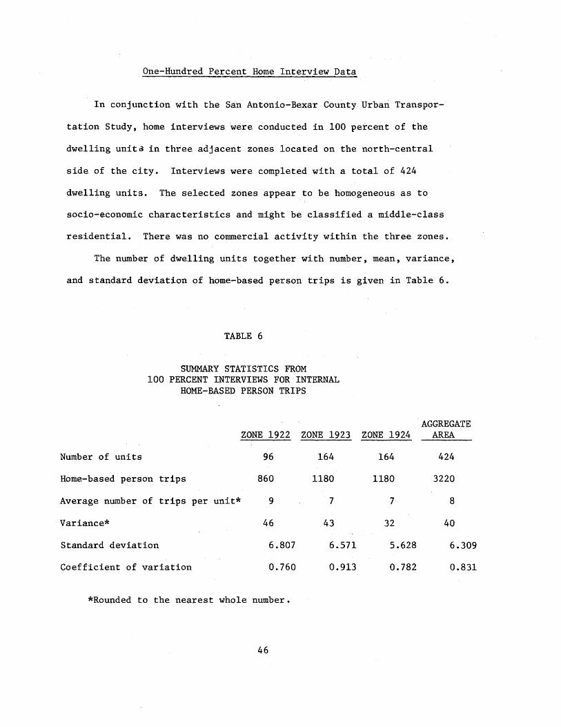
One-Hundred Percent Home Interview Data

In conjunction with the San Antonio-Bexar County Urban Transpor-

tation Study, home interviews were conducted in 100 percent of the

dwelling unit-a in three adjacent zones located on the north-central

side of the city. Interviews were completed with a total of 424

dwelling units. The selected zones appear to be homogeneous as to

socio-economic characteristics and might be classified a middle-class

residential. There was no commercial activity within the three zones.

The number of dwelling units together with number, mean, variance,

and standard deviation of home-based person trips is given in Table 6.

TABLE 6

SUMMARY STATISTICS FROM 100 PERCENT INTERVIEWS FOR INTERNAL

HOME-BASED PERSON TRIPS

ZONE 1922 ZONE 1923

Number of units 96 164

Home-based person trips 860 1180

Average number of trips per unit* 9 7

Variance* 46 43

Standard deviation 6.807 6.571

Coefficient of variation 0.760 0.913

*Rounded to the nearest whole number.

46

AGGREGATE ZONE 1924 AREA

164 424

1180 3220

7 8

32 40

5.628 6.309

0.782 0.831

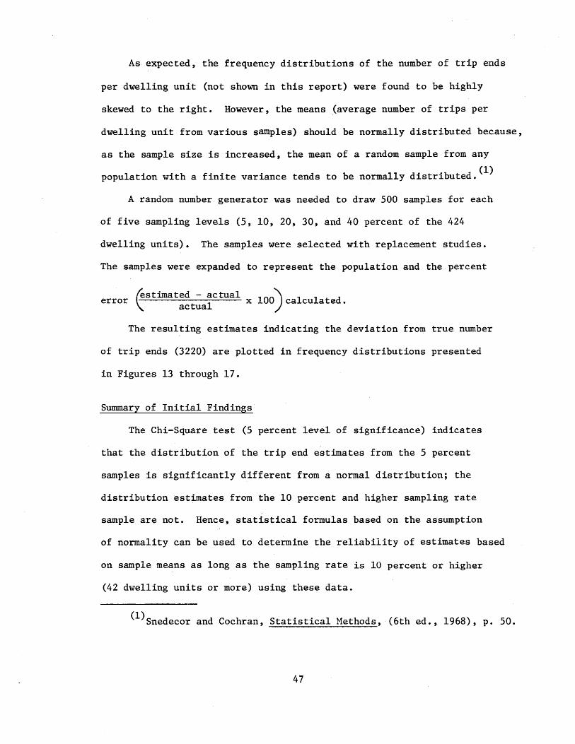
As expected, the frequency distributions of the number of trip ends

per dwelling unit (not shown in this report) were found to be highly

skewed to the right. However, the means (average number of trips per

dwelling unit from various samples) should be normally distributed because,

as the sample size is increased, the mean of a random sample from any

population with a finite variance tends to be normally distributed. (l)

A random number generator was needed to draw 500 samples for each

of five sampling levels (5, 10, 20, 30, and 40 percent of the 424

dwelling units). The samples were selected with replacement studies.

The samples were expanded to represent the population and the percent

~stimated - actual ) error 1

x 100 calculated. actua

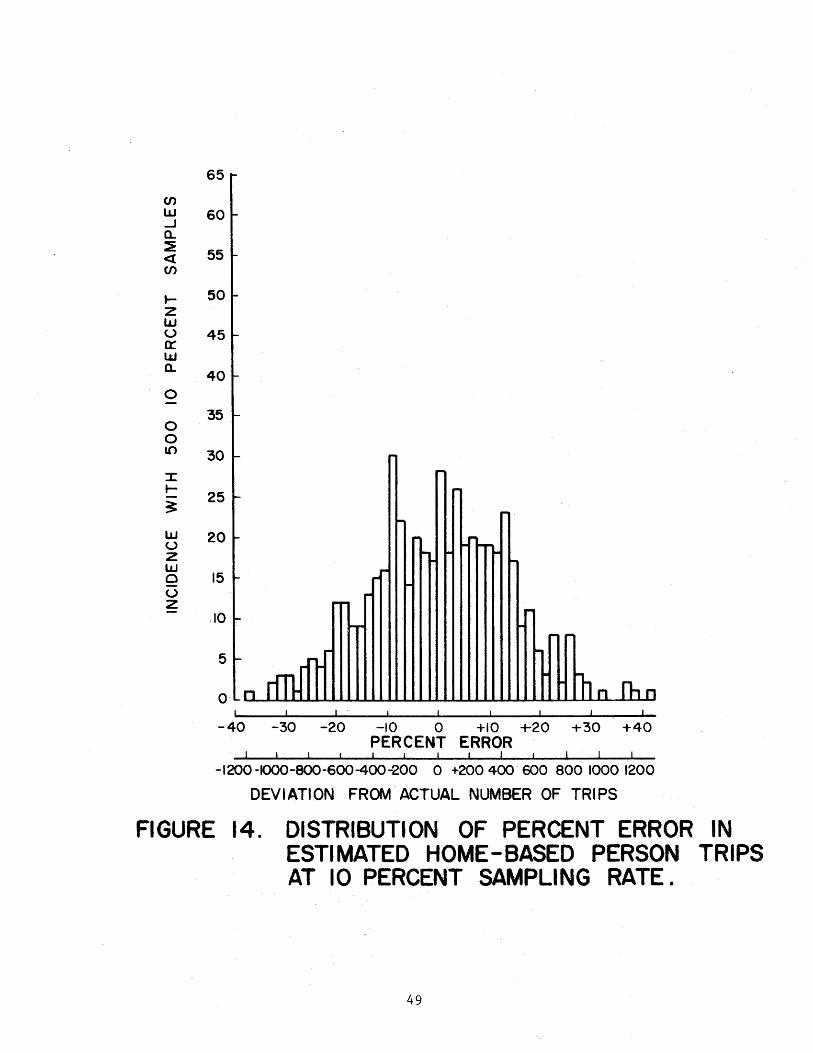
The resulting estimates indicating the deviation from true number

of trip ends (3220) are plotted in frequency distributions presented

in Figures 13 through 17.

Summary of Initial Findings

The Chi-Square test (5 percent level of significance) indicates

that the distribution of the trip end estimates from the 5 percent

samples is significantly different from a normal distribution; the

distribution estimates from the 10 percent and higher sampling rate

sample are not. Hence, statistical formulas based on the assumption

of normality can be used to determine the reliability of estimates based

on samplemeans as long as the sampling rate is 10 percent or higher

(42 dwelling units or more) using these data.

(l)Snedecor and Cochran, Statistical Methods, (6th ed., 1968), p. 50.

47

CJ)

UJ 45 _. Q. :E <( 40 CJ)

~ 35

Lt: 30 ~ It) 25

~ 20

:I: 1- 15 ~

UJ 10 0 z ~ 5 u z

0

-50 -40 -30 -20 -10 0 +10 +20 +30 +40 +50 +60 PERCENT ERROR

-1400-1200-1000-800-600-400-200 0 +200 400 600 800 1000 1200 1400 1600 1800

DEVIATIONS FROM ACTUAL NUMBER OF TRIPS

FIGURE 13. DISTRIBUTION OF PERCENT ERROR IN ESTIMATED HOME -BASED PERSON TRIPS AT 5 PERCENT SAMPLING RATE.

48

U)

lLJ ...J Q.

~ <t U)

...... z lLJ u 0:: lLJ Q.

0

0 0 lO

:c ...... ~

LU u z lLJ 0 u z

65

60

55

50

45

40

35

30 ~

P-

.. 25

~

~

20 I'" P"'

"" .,.. - - ~

~

15 P"'

I'" ~ -P"'-

P"'

-- "" - P"'

5

0

~ ~ -nrmf

~

"" rhn fh n

-40 -30 -20 -10 0 +10 +20 +30 +40 PERCENT ERROR

-1200-1000-800-600-400-200 0 +200 400 600 800 1000 1200

DEVIATION FROM ACTUAL NUMBER OF TRIPS

FIGURE 14. DISTRIBUTION OF PERCENT ERROR IN ESTIMATED HOME-BASED PERSON TRIPS AT 10 PERCENT SAMPLING RATE.

49

65

60

55 V> IJJ ...J Cl. 50 :E ~

45 1-z lLJ u 40 a: ~

lLJ ~

0... -35 r-

0 C\1

-1-

0 30 0

"' :r: t--~ IJJ u z IJJ 0 0 ~

~

- ""' "'" 25

20 ~ •r-

15 ... "" -

10 ~ .. ~ -

""' ~

5 ~ !"" 1- -

0 rf 1m, -30 -20 -10 0 +10 .+20 +30

PERCENT ERROR

-1000-800-600-400-2 00 0 200 400 600 800 I 000

OEVtATION FROM ACTUAL NUMBER OF TRIPS

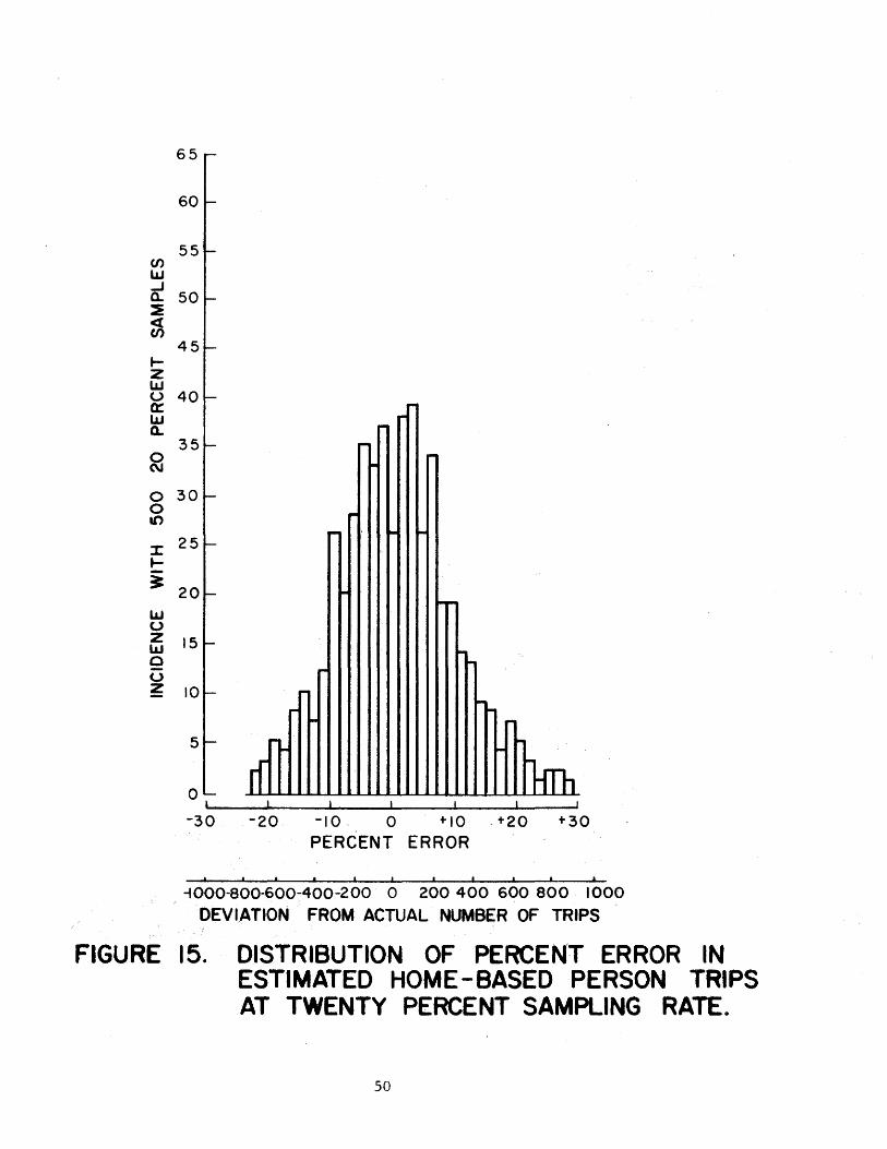
FIGURE 15. DISTRIBUTION OF PERCENT ERROR IN ESTIMATED HOME-BASED PERSON TRIPS AT TWENTY PERCENT SAMPLING RATE.

50

(/) UJ ..J

65

60

55

Q. 50 :E <[. CJ)

45 t-z UJ ~40 UJ Q.

0 35 rt)

g 30

iE 25

~

UJ 20 u z ~ 15 u ~

10

5

0

1--

1--

I-

1--

~

I--

~

I--

1--

I--

:- n r I

I"'

r-

1-

,.

... ...

1-

- 1-

·- --

-,..

"' ... ""

mh,n I I I I I

-30 -20 -10 0 + 10 +20 -t30

PERCENT ERROR

-800 -600-400 -200 0 +200 -t-400 1'600 +800

DEVIATION FROM ACTUAL NUMBER OF TRIPS

FIGURE 16. DISTRIBUTION OF PERCENT ERROR IN ESTIMATED HOME-BASED -PERSON TRIPS AT THIRTY PERCENT SAMPLING RATE.

51

CJ) w _J a.. ::E <( CJ)

t-z w u 0::: l&J a..

0 v 0 0 l{)

:I: t-~

w u z w 0 u z

65

60 ~

55 -..

50 i-

45

40 i-

35 ,... r""'

30

-25 ~ ..

-20 ~

1-

15 ~

1-

10 ~

- -5 ~

0 rf lh n

-30 -20 -10 0 -10 -20 -30 PERCENT ERROR

I I I I I I I -soo~4oo-2oo o +200+4oo+soo

DEVIATIONS FROM ACTUAL NUMBER OF TRIPS

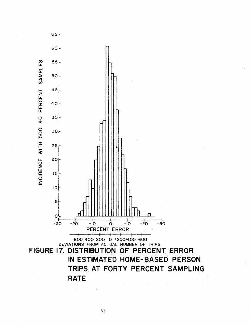
FIGURE 17. DISTRIBUTION OF PERCENT ERROR IN ESTIMATED HOME-BASED PERSON TRIPS AT FORTY PERCENT SAMPLING

RATE

52

The hypotheses of equal means and equal variances for the three

zones were also tested (home based person trips, home based auto driver

trips, home based work auto driver, and home based nonwork auto driver).

Statistical tests indicated that the hypotheses can be accepted and the

95 percent confidence level for all except the variances for homebased work

auto driver trips.

Based on the assumption of normality, the following formulas( 2)

were used to calculate the sample size needed to accurately estimate

the total number of trip ends:

n = 0

where, N t

s d n

0 n

=

=

=

(NtS) 2

(d)2 and

the size of the zone being sampled

n n

0

n 1 + __ o_

N

the value from the normal table which corresponds to the desired level of confidence, eg., 1.96 for 95% standard deviation desired degree of accuracy, eg., ± 322 trips. uncorrected sample size sample size after correction

The second formula corrects for finite populations. The sample size

needed to attain the desired degree of accuracy is given by n. For

example, in order to be 95 percent confident that the estimated total

number of trip ends will be within 10 percent of the actual number

generated by the 424 .dwelling units interviewed, a sample of 163

(40%) interviews would be needed.

n = 0

n =

(424 X 1.96 X 6.309) 2

(322) 2

265 ---= 163 1 + 265

424

265

(2)William G. Cochran, Sampling Techniques, John Wiler & Sons, 1963, p. 76.

53

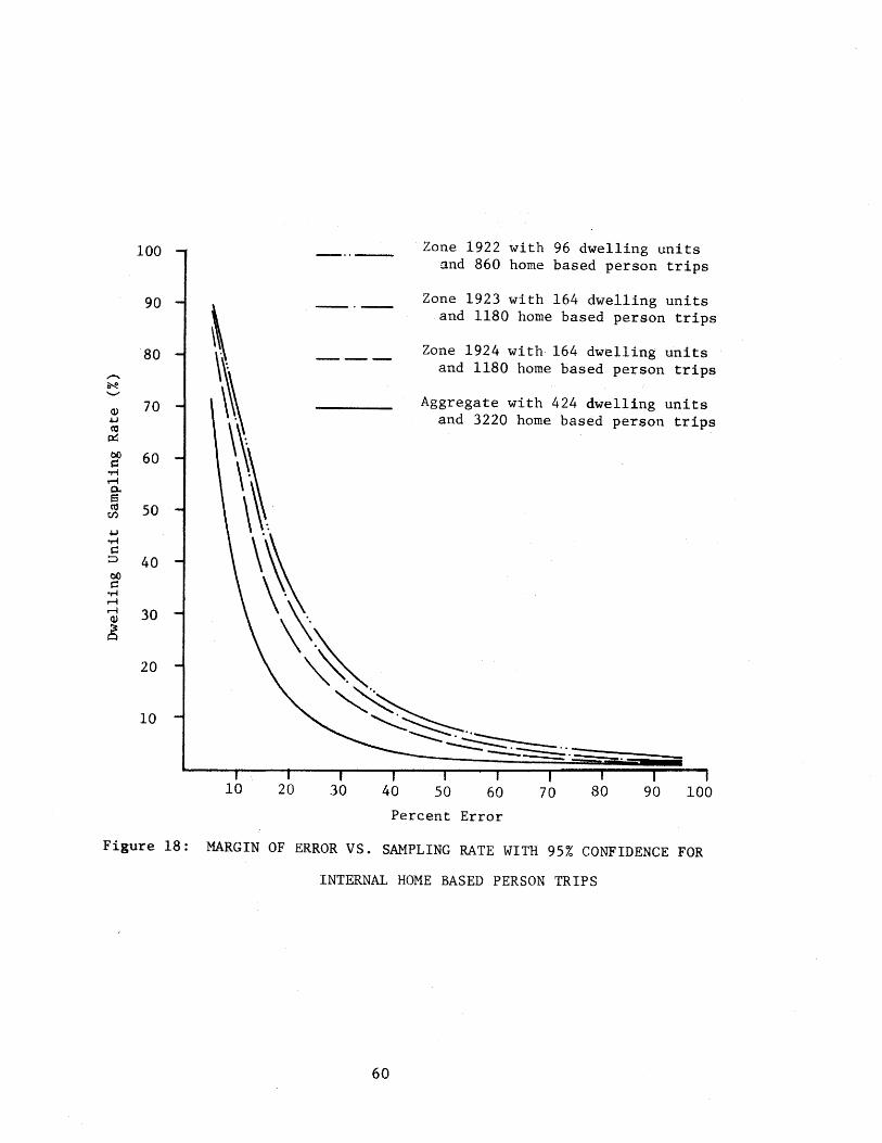
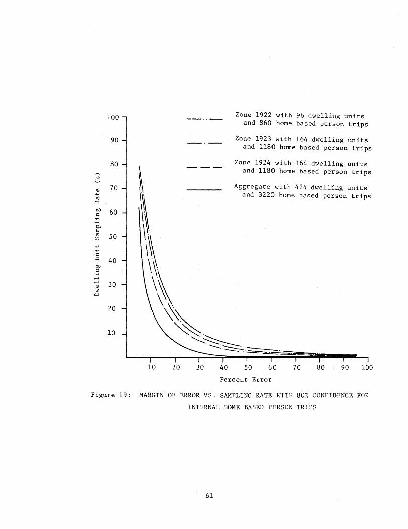
Calculations were made for each of the zones and for the aggregate,

at confidence levels of 95% and 80%; results are represented graphically

in Figures 18 and 19 respectively. These figures indicate that unexpect­

edly high sampling rates would be needed in order to estimate the total

number of trip ends with desirable accuracy. For example, a sampling

rate of over 20 percent is required in order to estimate the total number

of trip ends within plus/minus 10 percent at the 80 percent confidence

level.

A similar analysis was performed for internal home based auto driver

trips, internal home based work auto driver trips, and internal home

based nonwork auto driver trips. Tables 7, 8, and 9 contain the summary

statistics for these trips. Figures 20 through 26 illustrate the margin

of error versus the sampling rate for these trips _at confidence levels

of 95% and 80%.

Again, these figures indicate that unexpectedly high sampling rates

would be needed in order to estimate the total number of trip ends with

desirable accuracy. For example, a sample of nearly 20 percent would

be required to estimate the total number of horne based auto driver trip

ends within plus/minus 10 percent at the 80 percent confidence level.

Likewise, with the desired accuracy of plus/minus 10 percent at the 80

percent confidence level, a sampling rate of just under 20 percent would

be required to estimate the total number of horne based work auto driver trip

ends and the total number of horne based nonwork trip ends.

It is interesting to note .that a smaller sampling rate is required

to estimate the horne based auto driver trip ends than the home based

54

person trips. This indicates that, at any given sampling rate, the home-

based auto driver trip ends can probably be more accurately estimated than

the home-based person trip ends.

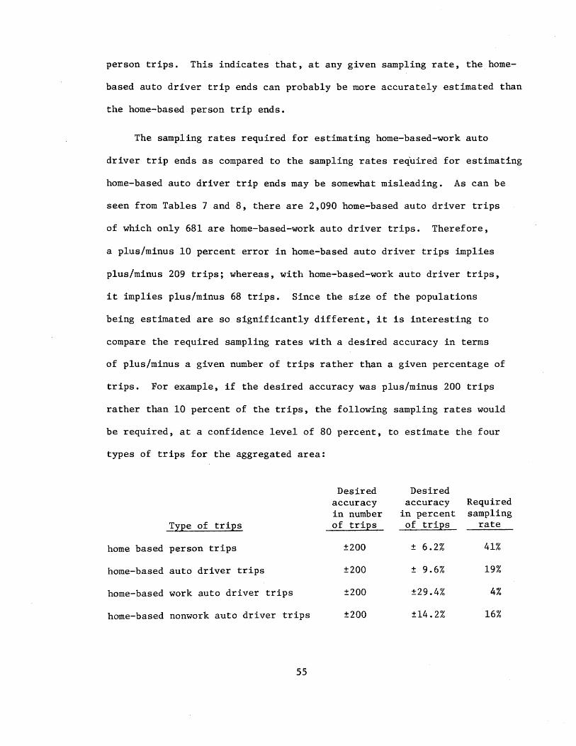
The sampling rates required for estimating home-based-work auto

driver trip ends as compared to the sampling rates required for estimating

home-based auto driver trip ends may be somewhat misleading. As can be

seen from Tables 7 and 8, there are 2,090 home-based auto driver trips

of which only 681 are home-based-work auto driver trips. Therefore,

a plus/minus 10 percent error in home-based auto driver trips implies

plus/minus 209 trips; whereas, with home-based-work auto driver trips,

it implies plus/minus 68 trips. Since the size of the populations

being estimated are so significantly different, it is interesting to

compare the required sampling rates with a desired accuracy in terms

of plus/minus a given number of trips rather than a given percentage of

trips. For example, if the desired accuracy was plus/minus 200 trips

rather than 10 percent of the trips, the following sampling rates would

be required, at a confidence level of 80 percent, to estimate the four

types of trips for the aggregated area:

Desired Desired accuracy accuracy Required in number in percent sampling

Type of trips of trips of trips rate

home based person trips ±200 ± 6.2% 41%

home-based auto driver trips ±200 ± 9.6% 19%

home-based work auto driver trips ±200 ±29.4% 4%

home-based nonwork auto driver trips ±200 ±14.2% 16%

55

A comprehensive analysis of the 100 percent data relative to both

trip ends and travel patterns is continuing under study 2-10-71-167.

conclusion

The preliminary findings of the 100 percent interviews and other

analyses suggest that the conduct of urban transport~tion studies might

be made more cost effective through the employment of "synthetic" study

techniques combined with data collection procedures designed to answer

specific questions and/or to fill particular "data gaps 11• (Such an

approach has been approved for and is being implemented with the Houston­

Galveston Area Urban Transportation Study.)

56

TABLE 7

SUMMARY STATISTICS FROM 100 PERCENT INTERVIEWS FOR INTERNAL

HOME-BASED AUTO DRIVER TRIPS

ZONE 1922 ZONE 1923

Number of units 96 164

Home-based auto driver trips 563 764

Average number of trips per unit* 6 5

Variance* 15 14

Standard deviation 3.911 3.760

Coefficient of variation 0.667 0.807

*Rounded to nearest whole number.

57

AGGREGATE ZONE 1924 AREA

164 424

763 2090

5 5

12 14

3.500 3.723

0.752 0.755

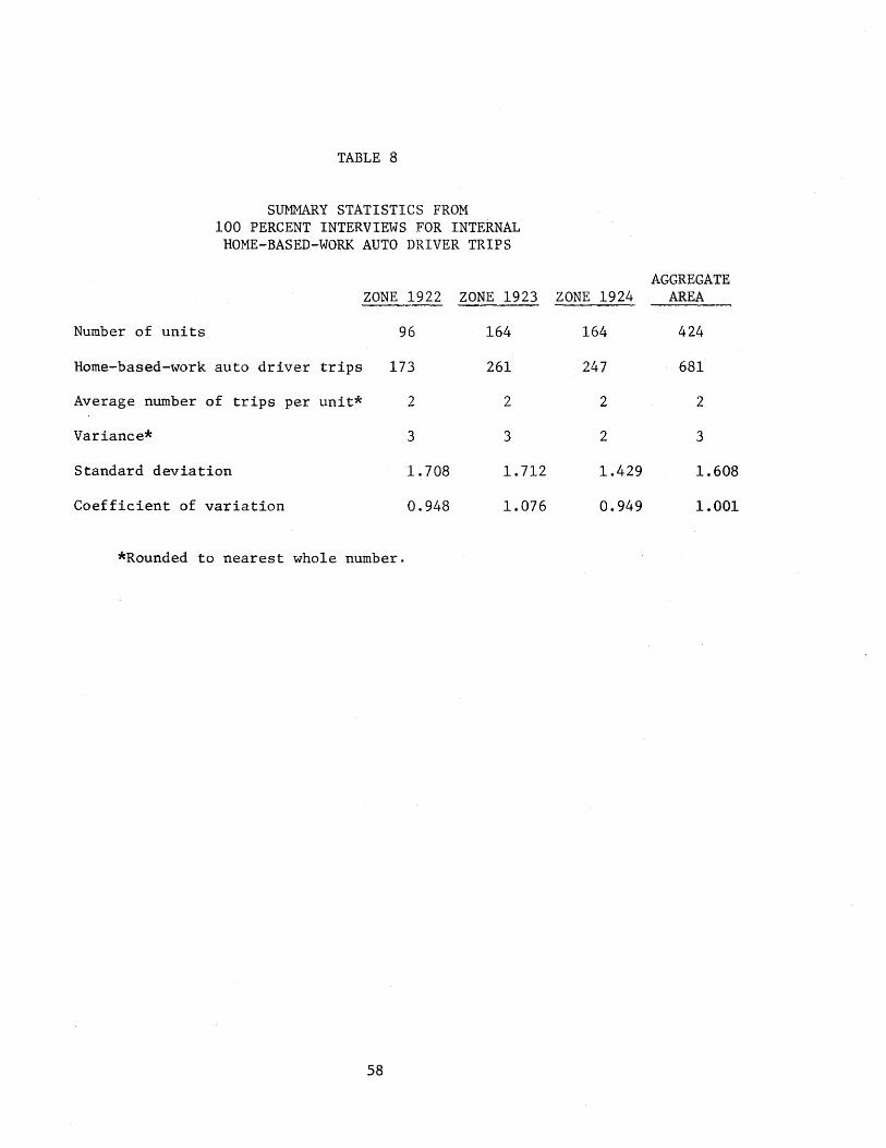
TABLE 8

SUMMARY STATISTICS FROM 100 PERCENT INTERVIEWS FOR INTERNAL

HOME-BASED-WORK AUTO DRIVER TRIPS

AGGREGATE ZONE 1922 ZONE 1923 ZONE 1924 AREA

Number of units 96 164 164 424

Home-based-work auto driver trips 173 261 247 681

Average number of trips per unit* 2 2 2 2

Variance* 3 3 2 3

Standard deviation 1.708 1.712 1.429 1.608

Coefficient of variation 0.948 1.076 0.949 1.001

*Rounded to nearest whole number.

58

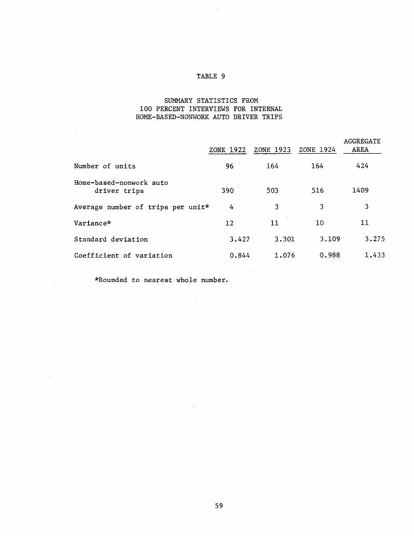
TABLE 9

SUMMARY STATISTICS FROM 100 PERCENT INTERVIEWS FOR INTERNAL

HOME-BASED-NONWORK AUTO DRIVER TRIPS

AGGREGATE ZONE 1922 ZONE 1923 ZONE 1924 AREA

Number of units 96 164 164 424

Home-based-nonwork auto driver trips 390 503 516 1409

Average number of trips per unit* 4 3 3 3

Variance* 12 11 10 11

Standard deviation 3.427 3.301 3.109 3.275

Coefficient of variation 0.844 1.076 0.988 1.433

*Rounded to nearest whole number.

59

100

90

80 ,....... il'-!! '-"

Q) 70 .u Cd

,:X:

bO 60 c:: "r'l ...-4 0.. s Cd 50 en .u ~ c::

:;::l 40 bO c:: ·~ ...-4 ...-4 30 Q)

~

20

10

10 20 30 40

Zone 1922 with 96 dwelling units and 860 home based person trips

Zone 1923 with 164 dwelling units and 1180 home based person trips

Zone 1924 with 164 dwelling units and 1180 home based person trips

Aggregate with 424 dwelling units and 3220 home based person trips

50 60 70 80 90 100

Percent Error

Figure 18: MARGIN OF ERROR VS. SAMPLING RATE WITH 95% CONFIDENCE FOR

INTERNAL HOME BASED PERSON TRIPS

60

100

90

80 ,......., b~ ..._...

(l) 70 +J C1:l ~

bO 60 c:: •.-i rl 0.. s ('lj 50 C/)

+J •.-i c::

;:J 40 bO c::

•.-i rl rl 30 (l)

~ 0

20

10

10 20 30 40

Zone 1922 with 96 dwelling units and 860 home based person trips

Zone 1923 with 164 dwelling units and 1180 home based person trips

Zone 1924 with 164 dwelling units and 1180 home based person trips

Aggregate with 424 dwelling units and 3220 home based person trips

50 60 70 80 90 100

Percent Error

Figure 19: MARGIN OF ERROR VS. SAMPLING RATE HITH 80% CONFIDENCE FOR

INTERNAL HOME BASED PERSON TRIPS

61

Zone 1922 with 96 dwelling units 100 --··-- and 563 home based auto driver trips

Zone 1923 with 164 dwelling units and 90 -·- 764 home based auto driver trips

\ Zone 1924 with 164 dwelling units

80 -'-- and 763 home based auto driver trips "'""" IN! '-"

Aggregate with 424 dwelling units QJ 70 and 2090 home based auto driver trips ~

~ ctl ~

bO

~: ~ 60 .,.... rl 0.. s (lj lfj 50

\~ ~ •.-I ~

;::J 40 bO

\~ ~ ·.-I .....-!

~. .....-! QJ 30 ~

Cl \\ 20 \~ ~~ 10 ~-. ~---===-·

10 20 30 40 50 60 70 80 90 100

Percent Error

Figure 20: ~~RGIN OF ERROR VS. SAMPLING RATE WITH 95% CONFIDENCE FOR

INTERNAL HOME BASED AUTO DRIVER TRIPS

62

100 Zone 1922 \vith 96 dwelling units and 563 home based auto driver trips

90 Zone 1923 with 164 dwelling units -·- and 764 home based auto driver trips

80 Zone 1924 with 164 dwelling units ,-.. and 763 home based auto driver trips N '-"

Q) 70 Aggregate with 424 dwelling units +J m and 2090 home based auto driver trips

p::

0.0 60 ~ -r1 ......., 0.. s m 50 C/)

+J •ri ~

:::> 40 b.()

~ •ri ......., .......,

30 Q)

~ ~

20

10

10 20 30 40 50 60 70 80 90 100

Percent Error

Figure 21: MARGIN OF ERROR VS. S&~PLING RATE WITH 80% CONFIDENCE FOR

INTERNAL HOME BASED AUTO DRIVER TRIPS

63

Zone 1922 with 96 dwelling units and 100 --··-- 173 home based work auto driver

90 }. Zone 1923 with 164 dwelling units --·-- 261 home based work auto driver

Zone 1924 with 164 dwelling units 80 ~ --- 247 home based work auto driver ,...._ ~ ............

~' Aggregate with 424 dwelling units 70 <1l 681 home based work auto driver +J

a:!

~\ ex: ()()

60 c ·r-l ~

~-\ p,. s m

50 U)

+.J •r-l s:: \\ :.::>

40 ()()

t:: \·~ •r-l ~ ~

<1l 30 ) \-~ 0

20 ~~ ~-~-- .

10 ~-~ ~-·· -----;:;;:.:;;.

Percent Error

Figure 22: MARGIN OF ERROR VS. SAMPLING RATE WITH·95% CONFIDENCE FOR

INTERNAL HOME BASED WORK AUTO DRIVER TRIPS

64

trips

and trips

and trips

and trips

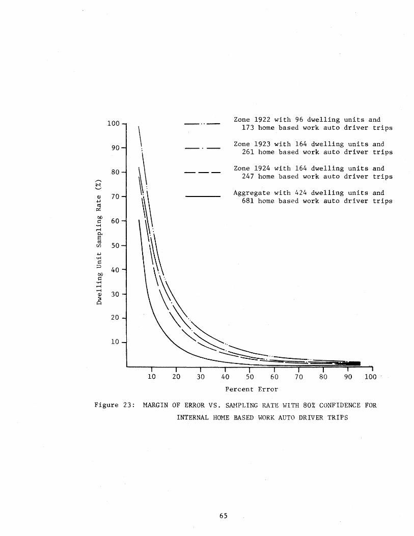
100 Zone 1922 with 96 dwelling units and _._,..... .. --

173 home based work auto driver trips

\ 90 Zone 1923 with 164 dwelling units and --·-- 261 home based work auto driver trips

~\ 80 Zone 1924 with 164 dwelling units and --- 247 home based work auto driver trips .......... ~ '-"

70

~ Aggregate with 424 dwelling units and

Cll 681 home based work auto driver trips +J ~ ~

bO 60 l=l

•ri .-I 0.. s C'O

50

~ U)

.1-J ·ri l=l

;::::l 40

bO

\~ l=l ·r-1 .-I .-I Cll 30 \\ ~ 0

20 ~ "'~ 10 ~··

~·· ~.

10 20 30 40 so 60 70 80 90 100

Percent Error

Figure 23: MARGIN OF ERROR VS. SA}1PLING RATE WITH 80% CONFIDENCE FOR

INTERNAL HOHE BASED WORK AUTO DRIVER TRIPS

65

Zone 1922 with 96 dwelling units and 100 390 home based nonwork auto driver trips

Zone 1923 with 164 dwelling units and 90 503 home based nonwork auto driver trips

Zone 1924 with 164 dwelling units and 80 516 home based nonwork auto driver trips

"""" ~ ..._

Aggregate with 424 dwelling units and Q) 70

.j..J 1409 home based nonwork auto driver trips cO

0:: ()()

~ 60 ·.-4 r-f 0.. s cO

CJ) 50 .j..J

"1""4 1=l ~

()() 40 ~

·.-4 r-f r-f Q) 30 ~ 0

20

10

10 20 30 40 50 60 70 80 90 100

Percent Error

Figure 24: }~RGIN OF ERROR VS. SAMPLING RATE WITH 95% CONFIDENCE FOR

INTERNAL HOME BASED NONWORK AUTO DRIVER TRIPS

66

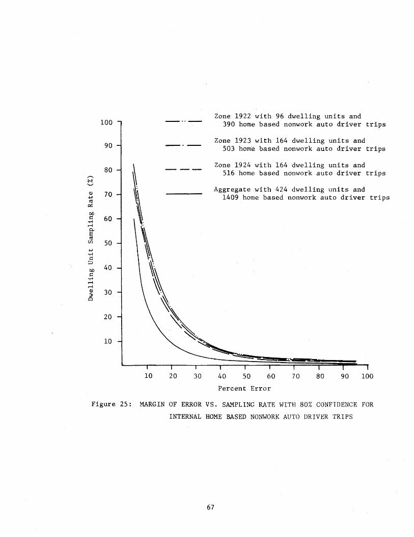
Zone 1922 with 96 dwelling units and 100 390 home based nonwork auto driver trips

90 Zone 1923 with 164 dw.elling units and

S03 home based nonwork auto driver trips

80 ,-...

Zone 1924 with 164 dwelling units and S16 home based nonwork auto driver trips

~ ........

<l) 70 +J (1j

Aggregate with 424 dwelling units and 1409 home based nonwork auto driver trips

~

bO ~ 60 ·~ r-1 p.. s (1j

(/) so +J ·~ ~ ~

bO 40 ~ ·~ r-1 r-1 <l) 30 6

20

10

10 20 30 40 so 60 70 80 90 100

Percent Error

Figure 2S: MARGIN OF ERROR VS. SAMPLING RATE WITH 80% CONFIDENCE FOR

INTERNAL HOME BASED NONWORK AUTO DRIVER TRIPS

67

APPENDIX

Study Objectives and Summary of Accomplishments

The objectives of Study 2-10-68-119, are stated below together

with a summary of the work accomplished and the status of each objective

at the end of August, 1970.

OBJECTIVE #1: Investigate techniques and develop procedure for making Traffic Assignments to small portions of large networks for the purpose of evaluating alternative route locations and/or designs that are relatively localized in terms of the size of the entire study area.

Accomplishments/Status:

Work was initiated on this objective in the first year of the study (1967-68). The procedures and computer programs were based upon programs that were originally developed under research sponsored by the Bureau of Public Roads. These programs would assemble small coded areas (with the desired degree of detail in each) into an assignment network. However, work was temporarily halted shortly after initial conversion of the IBM 7094 programs to the IBM 360 System was undertaken. Decision to halt work was based on the fact that this program capability was not then essential whereas other computer program capabilities were immediately needed for the day-to-day operation of the Planning Survey Division. No work was performed on the objective in Fiscal Year 1968-69. During this time, analysis of the San Antonio and Houston/Galveston Transportation Network indicated critical problems in the establishment of partition lines necessary for small area coding in these two study areas. It was, therefore, agreed to permanently suspend work on this objective with the recommendation that the objective be officially terminated and removed from the scope of work.

Completion: The objective was terminated.

68

OBJECTIVE #2: Test and evaluate the capacity/volume restrained program developed under Study Number 2-8-63-60.

Accomplishments/Status:

The restrained assignment procedure was developed as a set of stand alone programs to facilitate development and testing independent of the assignment packages being used by the Texas Highway Department. Restrained assignment capability was added to the Small Network and Large Network Assignment Packages after the initial evaluation by the Highway Department indicated that the procedure provided acceptable and useful results. Two versions of the draft of the research report concerning the development of the restrained assignment procedure were reviewed by the Texas Highway Department Planning Survey Division. However, this report has not been finalized because substantial effort needed to be diverted to more critical problems relative to continued day-to-day operation of the Highway Department. Further, the documentation was not considered essential due to the fact that Highway Department personnel were familiar with the procedure by virtue of close liaison throughout the development.

First application of the restrained assignment procedure was made in conjunction with the McAllen-Pharr Urban Transportation Study.

Completion: Writeups for executing the restrained assignment procedure were incorporated in the operating manuals for the two traffic assign­ment reports (119-1 and 119-2). Documentation of the development and evaluation will be completed under Study Number 2-10-71-167.

OBJECTIVE /13: Program, Test, and evaluate the THD trip distribution forecasting procedure outlined under Study Number 2~8-63-60.

Accomplishments/Status:

The THD Trip Distribution Model was developed as a package of computer programs and subroutines. Initial use of the package by the Texas Highway Department led to a variety of modifications and numerous programming corrections. The McAllen-Pharr Urban Transportation Study was used as the primary basis for test and evaluation of the THD Trip Distribution Procedure. Satisfactory performance led to its general adoption by the Highway Department as the trip distribution procedure used in urban transportation studies in Texas and was first applied in an operational manner in the El Paso Urban Transportation Study.

Completion: A manual for executing the package together with a report concerning the development and testing of the procedure will be prepared under Study Number 2-10-71-167.

69

OBJECTIVE #4: Evaluate the accuracy of nonhome trip end (attraction) information.

Accomplishments/Status:

The accuracy of nonhome trip information from the conventional 0-D Survey was evaluated using data from the McAllen-Pharr Urban Transportation Study. The results and evaluation of the comparisons made were reported in a technical memorandum. It was further concluded that little, if any, benefit might be gained from more extensive work using additional data from other urban transportation studies, and that more valuable results might be obtained from other analyses such as that of the 100% home interview data collected in the San Antonio-Bexar County Urban Transportation Study.

Completion: Issuance of a technical memorandum entitled, "Accuracy of Employment and Nonhome Trip End Estimates From the Home Interview" dated 15 September 1969. Correspondence from D-8 Research dated 12 December, 1969 stated that the technical memorandum satisfactorily completed this objective and that no further report(s) was necessary.

OBJECTIVE #5: Investigate techniques for analyzing and/or statistically evaluating the data collection projection and assignment phases of transportation studies separately or in combination.

Accomplishments/Status:

At the outset of the research it was hopeful that statistical measurement techniques applicable to urban transportation studies might be developed from statistical theory. However, continued contact and inquiry with members of the staff of the Institute of Statistics at Texas A&M University failed to develop potentially successful avenues of research. It was therefore decided to dis­continue further attempts in this direction and to concentrate on the application of existing statistical procedures. A variety of comparisons and applications of statistical tests were incorporated into the output of the Assignment Packages and the Trip Distribution Package. The potential value of this output is still in question and can probably be determined only through attempts at application in the day-to-day conduct of several urban transportation studies.

Completion: Agreement to not pursue the theoretical approach further and to incorporate· routines to provide statistical summary data into the appropriate computer programs and packages developed under Objectives 3 and 6.

70

OBJECTIVE #6: Investigate and develop a partition- simultaneous tree building and network coding procedure.

Accomplishments/Status:

Two Traffic Assignment Packages were developed for the IBM 360 System for use by the Texas Highway Department. Both packages were designed to use input and provide output similar to that for the IBM 7094 Package previously used by the Texas Highway Department; problems that resulted from changing from the IBM 7094 to the IBM 360 System were therefore minimized. Development of what has become known as the Small Network Assignment Package was developed and tested by the end of December, 1967; this package was adopted as the Operational Traffic Assignment Program Package of the Texas Highway Department in January, 1968. This package of programs is for application with study areas having networks of less than 4,000 nodes; it uses a procedure whereby minimum paths are searched and the network is loaded simultaneously.

A battery of programs were then developed to enable the Texas Highway Department to continue making the necessary assignments to the Dallas/Ft. Worth Network. These programs were initially a conversion of the IBM 7094 programs together with a program required to assemble the four separately coded subnets into a single network. Continued revisions and modifications have led to a package of programs called the Large Network Assignment Package which is used by the Highway Department for all coded networks containing more than 4,000 nodes.

This objective also includes the prov1s1on of such report as may be required to maintain and improve the computer programs used by the Texas Highway Department. In the course of the project numerous changes in the several programs were required to either correct errors or problems found in the operational use of the programs or to regain operational capability which was lost due to changes in the IBM 360 Operating System. Reprogramming necessitated because of changes in the IBM 360 Operating System were especially troublesome and time consuming.

Completion: Adoption of the program packages by the Planning Survey Division of the Texas Highway Department for operational use; and, the preparation of an operating manual for each package (Research Reports 119-1 and 119-2).

OBJECTIVE #7: Supply computer programming and analysis support to the Texas Highway Department concerning procedures developed and/or evaluated on Study Numbers 2-8-63-60 and 2-10-68-119.

71

Accomplishments/Status:

This objective was added in the third and final year of the study and was directed towards the identification of alternatives and less costly study procedures with particular interest in application to small study areas. Prior to the termination of Study Number 2-10-68-119 the possibility of applying less costly study procedures in large urban areas was seriously considered by the Texas Highway Department. Particular interest and concern centered on the proposed Houston/Galveston Urban Transportation Study. The decision to proceed with a significantly revised study design for the Houston/Galveston Study led t9 the continuation and transfer of this work to Study Number 2-10~71-167.

Completion: Transfer and continuation as Objective #3 of Study Number 2-10-71-167

72