Traffic: Monitoring, Estimation, and Engineering

Nick Feamster

CS 7260February 14, 2007

2

Administrivia

• Syllabus redux– More time for traffic monitoring/engineering– Simulation vs. emulation pushed back (Feb. 21)

• Workshop deadlines (6-page papers)– Reducing unwanted traffic: April 17– Large scale attacks: April 21– Network management: April 26– Include in your proposal whether you will aim for one

of these.

3

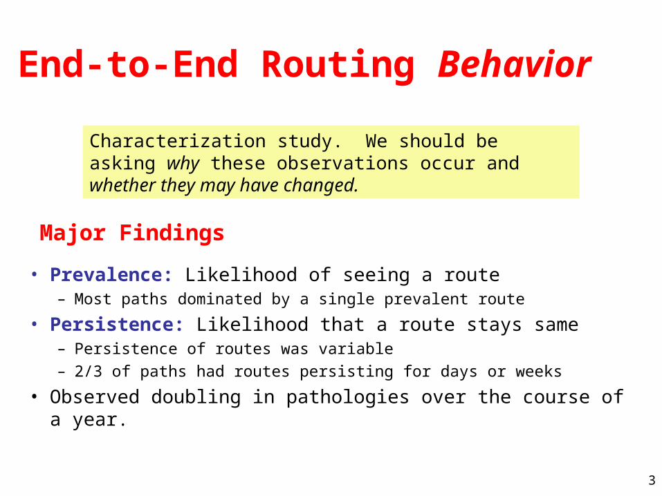
End-to-End Routing Behavior

• Prevalence: Likelihood of seeing a route– Most paths dominated by a single prevalent route

• Persistence: Likelihood that a route stays same– Persistence of routes was variable– 2/3 of paths had routes persisting for days or weeks

• Observed doubling in pathologies over the course of a year.

Major Findings

Characterization study. We should be asking why these observations occur and whether they may have changed.

4

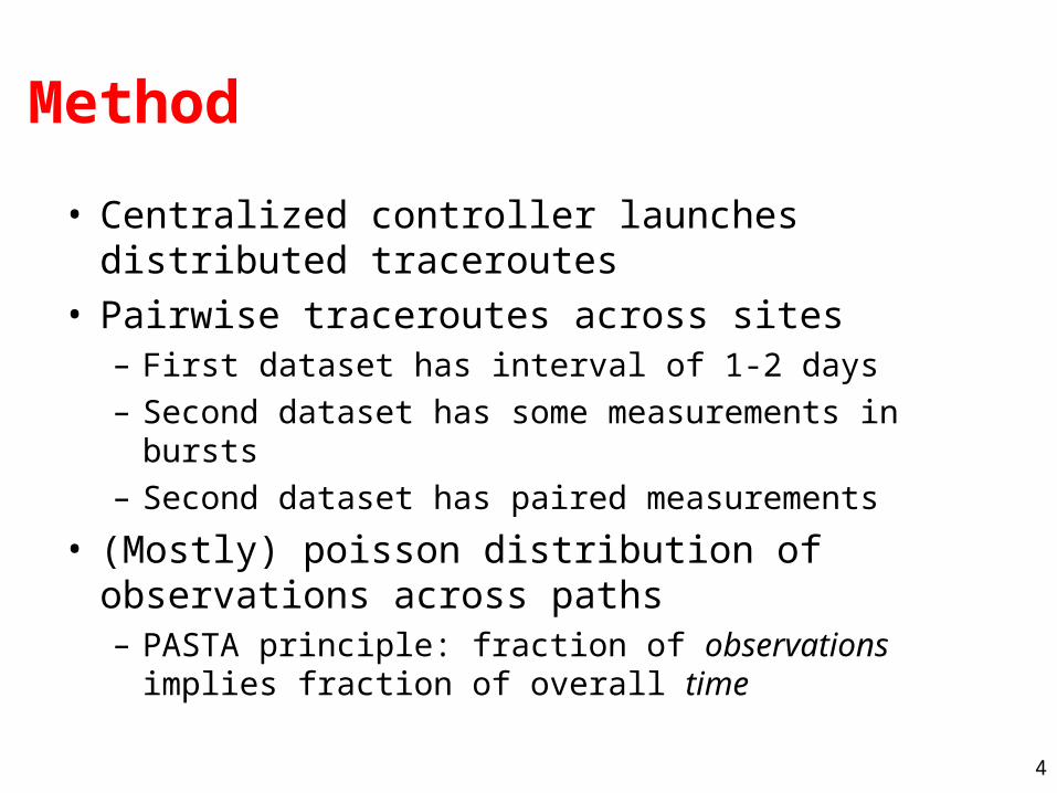
Method

• Centralized controller launches distributed traceroutes

• Pairwise traceroutes across sites– First dataset has interval of 1-2 days– Second dataset has some measurements in bursts– Second dataset has paired measurements

• (Mostly) poisson distribution of observations across paths– PASTA principle: fraction of observations implies

fraction of overall time

5

Arguing “Representativeness”

• Always tricky business…• This paper: fraction of ASes traversed by the

pairwise paths (8% “cross section”)• D1: ~ 7k traceroutes; D2: ~38k traceroutes• Assigning pathologies to a particular AS is

challenging

• No explanation of why or where.• Centralized controller limits flexibility• Traceroute issues

Limitations

6

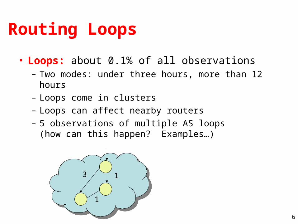
Routing Loops

• Loops: about 0.1% of all observations– Two modes: under three hours, more than 12 hours– Loops come in clusters– Loops can affect nearby routers– 5 observations of multiple AS loops

(how can this happen? Examples…)

1

1

3

7

Erroneous Routing

• Packets clearly taking wrong path (e.g., through Israel)

• One example of erroneous routing

8

Changing Paths

• Connectivity altered mid-stream– Between 0.16% and 0.44%– Recovery times bimodal– Cause

• Fluttering– Rapidly oscillating routing

• Load balance/splitting– Distinct from fluttering caused by routing oscillations?

9

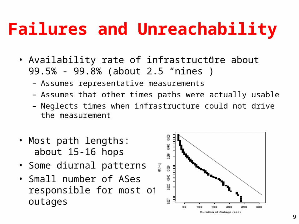
Failures and Unreachability

• Availability rate of infrastructure about 99.5% - 99.8% (about 2.5 “nines”)– Assumes representative measurements– Assumes that other times paths were actually usable– Neglects times when infrastructure could not drive the

measurement

• Most path lengths: about 15-16 hops

• Some diurnal patterns• Small number of ASes

responsible for most ofoutages

10

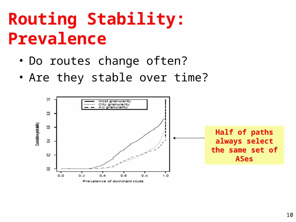
Routing Stability: Prevalence

• Do routes change often?• Are they stable over time?

Half of paths always select the same set

of ASes

11

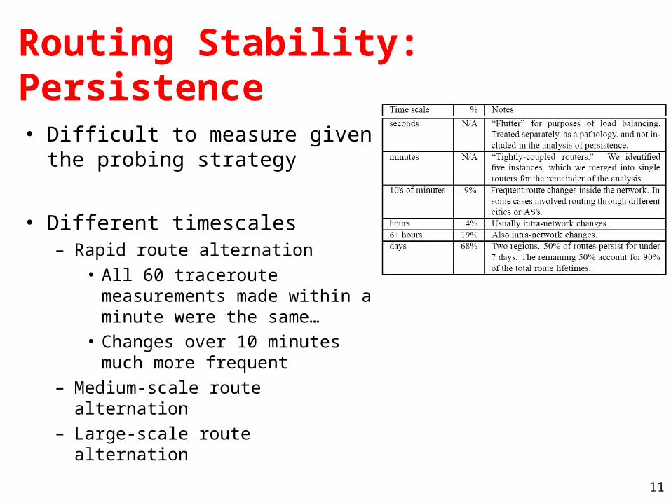
Routing Stability: Persistence

• Difficult to measure given the probing strategy

• Different timescales– Rapid route alternation

• All 60 traceroute measurements made within a minute were the same…

• Changes over 10 minutes much more frequent

– Medium-scale route alternation– Large-scale route alternation

12

Routing Symmetry

• Finding: 49% of measurements exhibit path asymmetry

• Causes– Hot-potato routing– Policy routing

• Hypothesis: Multihoming has increased the degree of routing symmetry

13

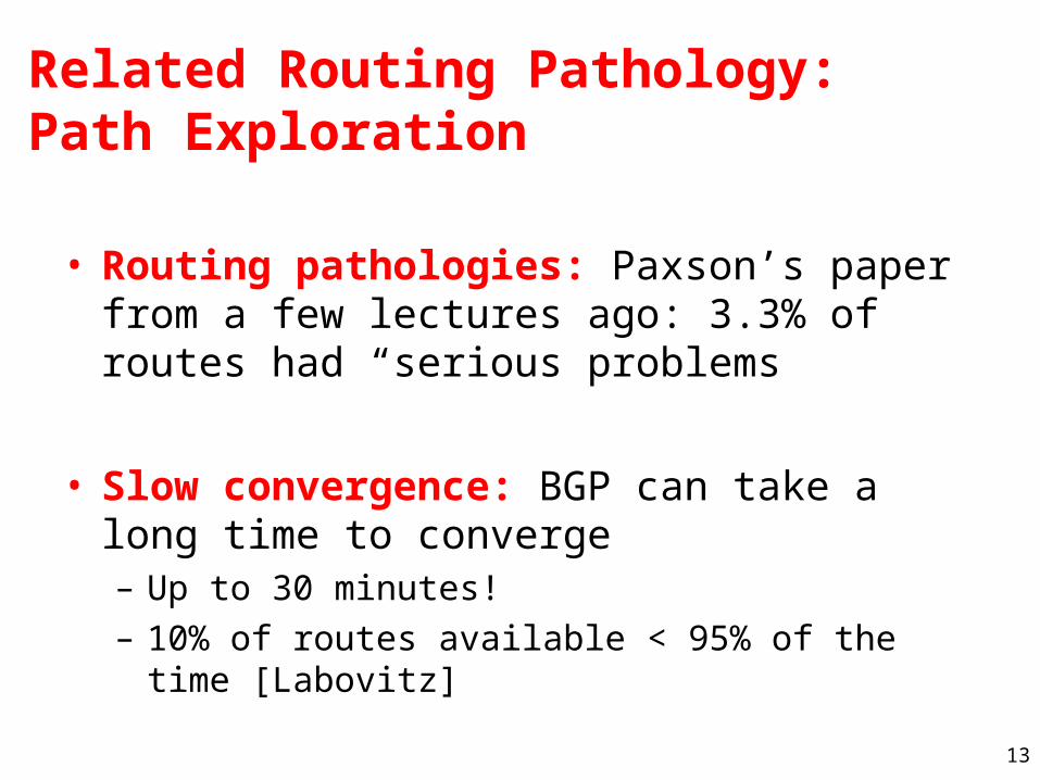
Related Routing Pathology: Path Exploration

• Routing pathologies: Paxson’s paper from a few lectures ago: 3.3% of routes had “serious problems

• Slow convergence: BGP can take a long time to converge– Up to 30 minutes!– 10% of routes available < 95% of the time [Labovitz]

14

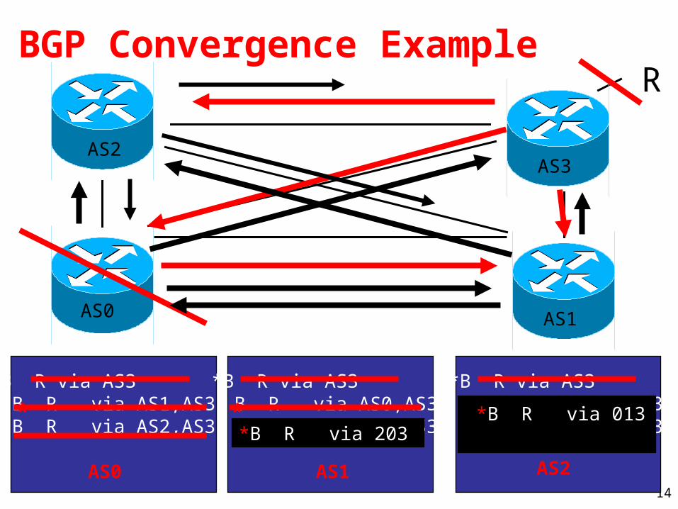
BGP Convergence ExampleR

AS0 AS1

AS2AS3

*B R via AS3 B R via AS0,AS3 B R via AS2,AS3

*B R via AS3 B R via AS0,AS3 B R via AS1,AS3

*B R via AS3 B R via AS1,AS3 B R via AS2,AS3

AS0 AS1 AS2

** **B R via 203

*B R via 013

15

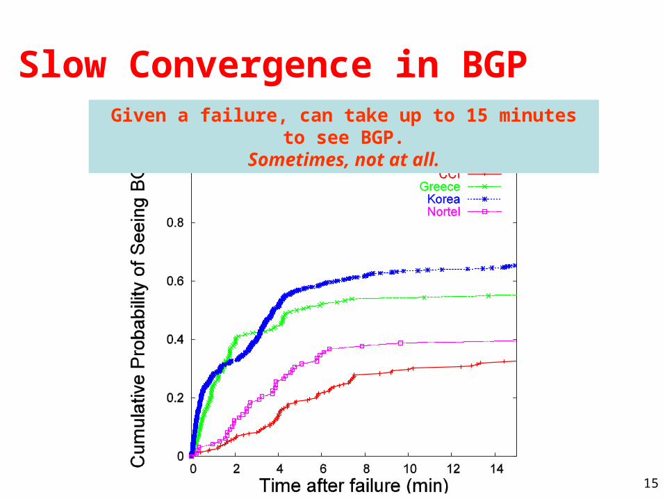
Slow Convergence in BGPGiven a failure, can take up to 15 minutes to see BGP.

Sometimes, not at all.

16

Intuition for Delayed BGP Convergence

• There exists a message ordering for which BGP will explore all possible AS paths

• Convergence is O(N!), where N number of default-free BGP speakers in a complete graph

• In practice, exploration can take 15-30 minutes• Question: What typically prevents this exploration

from happening in practice?

• Question: Why can’t BGP simply eliminate all paths containing a subpath when the subpath is withdrawn?

17

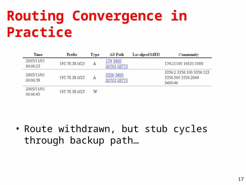
Routing Convergence in Practice

• Route withdrawn, but stub cycles through backup path…

18

Passive Measurement

19

Two Main Approaches

• Packet-level Monitoring– Keep packet-level statistics– Examine (and potentially, log) variety of packet-level

statistics. Essentially, anything in the packet.– Timing

• Flow-level Monitoring– Monitor packet-by-packet (though sometimes

sampled)– Keep aggregate statistics on a flow

20

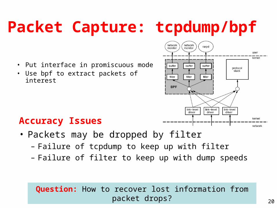
Packet Capture: tcpdump/bpf

• Put interface in promiscuous mode• Use bpf to extract packets of interest

• Packets may be dropped by filter– Failure of tcpdump to keep up with filter– Failure of filter to keep up with dump speeds

Question: How to recover lost information from packet drops?

Accuracy Issues

21

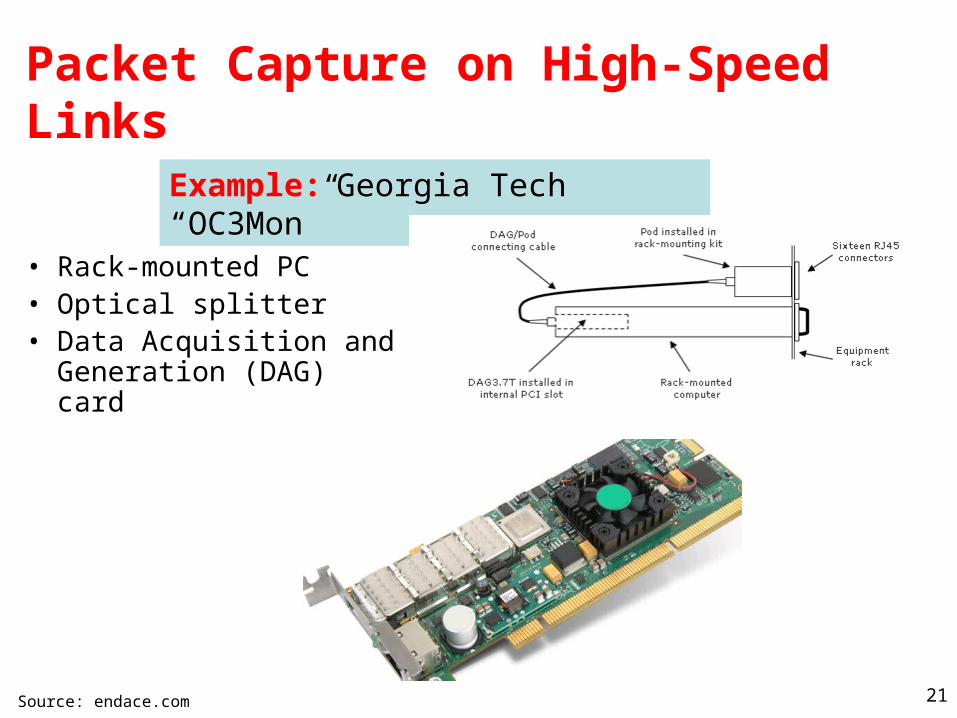
Packet Capture on High-Speed Links

Example: Georgia Tech “OC3Mon”

• Rack-mounted PC• Optical splitter• Data Acquisition and

Generation (DAG) card

Source: endace.com

22

Characteristics of Packet Capture

• Allows inpsection on every packet on 10G links

• Disadvantages– Costly– Requires splitting optical fibers– Must be able to filter/store data

23

Traffic Flow Statistics

• Flow monitoring (e.g., Cisco Netflow)– Statistics about groups of related packets (e.g., same

IP/TCP headers and close in time)– Recording header information, counts, and time

• More detail than SNMP, less overhead than packet capture– Typically implemented directly on line card

24

What is a flow?

• Source IP address• Destination IP address• Source port• Destination port• Layer 3 protocol type• TOS byte (DSCP)• Input logical interface (ifIndex)

25

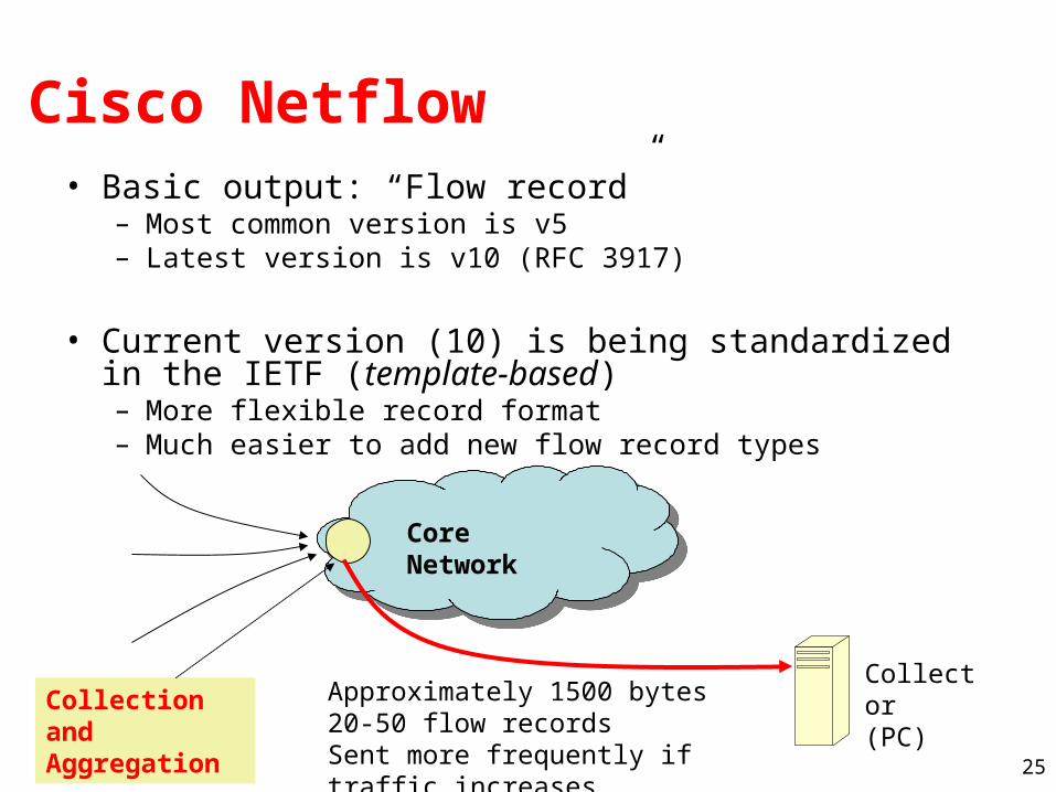
Cisco Netflow• Basic output: “Flow record”

– Most common version is v5– Latest version is v10 (RFC 3917)

• Current version (10) is being standardized in the IETF (template-based)– More flexible record format– Much easier to add new flow record types

Core Network

Collection and Aggregation

Collector (PC)Approximately 1500 bytes

20-50 flow recordsSent more frequently if traffic increases

26

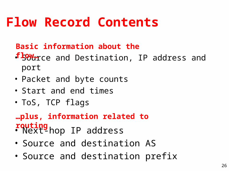
Flow Record Contents

• Source and Destination, IP address and port• Packet and byte counts• Start and end times• ToS, TCP flags

Basic information about the flow…

…plus, information related to routing

• Next-hop IP address• Source and destination AS• Source and destination prefix

27

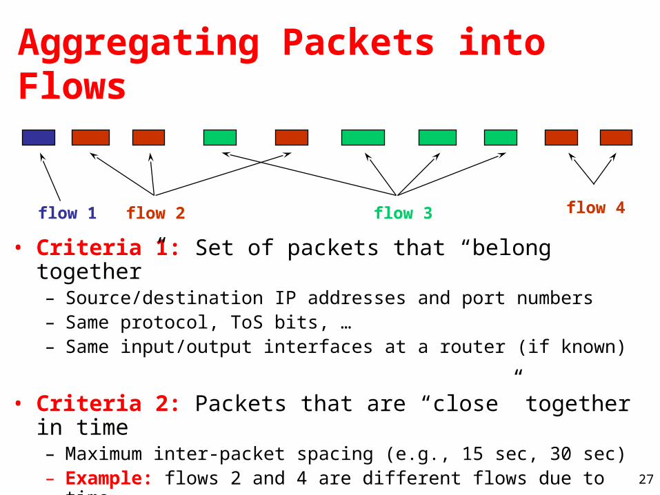
flow 1 flow 2 flow 3 flow 4

Aggregating Packets into Flows

• Criteria 1: Set of packets that “belong together”– Source/destination IP addresses and port numbers– Same protocol, ToS bits, … – Same input/output interfaces at a router (if known)

• Criteria 2: Packets that are “close” together in time– Maximum inter-packet spacing (e.g., 15 sec, 30 sec)– Example: flows 2 and 4 are different flows due to time

28

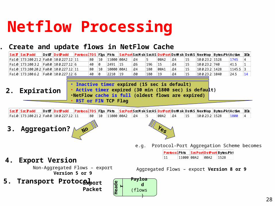
Netflow Processing1. Create and update flows in NetFlow Cache

• Inactive timer expired (15 sec is default)• Active timer expired (30 min (1800 sec) is default)•NetFlow cache is full (oldest flows are expired)• RST or FIN TCP Flag

He

ad

er

ExportPacket

Payload(flows)

2. Expiration

3. Aggregation?

Protocol Pkts SrcPort DstPort Bytes/Pkt

11 11000 00A2 00A2 1528

SrcIf SrcIPadd DstIf DstIPadd Protocol TOS Flgs Pkts SrcPort SrcMsk SrcAS DstPort DstMsk DstAS NextHop Bytes/Pkt Active Idle

Fa1/0 173.100.21.2 Fa0/0 10.0.227.12 11 80 10 11000 00A2 /24 5 00A2 /24 15 10.0.23.2 1528 1800 4

e.g. Protocol-Port Aggregation Scheme becomes

4. Export Version

SrcIf SrcIPadd DstIf DstIPadd Protocol TOS Flgs Pkts SrcPort SrcMsk SrcAS DstPort DstMsk DstAS NextHop Bytes/Pkt Active Idle

Fa1/0 173.100.21.2 Fa0/0 10.0.227.12 11 80 10 11000 00A2 /24 5 00A2 /24 15 10.0.23.2 1528 1745 4

Fa1/0 173.100.3.2 Fa0/0 10.0.227.12 6 40 0 2491 15 /26 196 15 /24 15 10.0.23.2 740 41.5 1

Fa1/0 173.100.20.2 Fa0/0 10.0.227.12 11 80 10 10000 00A1 /24 180 00A1 /24 15 10.0.23.2 1428 1145.5 3

Fa1/0 173.100.6.2 Fa0/0 10.0.227.12 6 40 0 2210 19 /30 180 19 /24 15 10.0.23.2 1040 24.5 14

YesNo

Aggregated Flows – export Version 8 or 9Non-Aggregated Flows – export Version 5 or 9

5. Transport Protocol

29

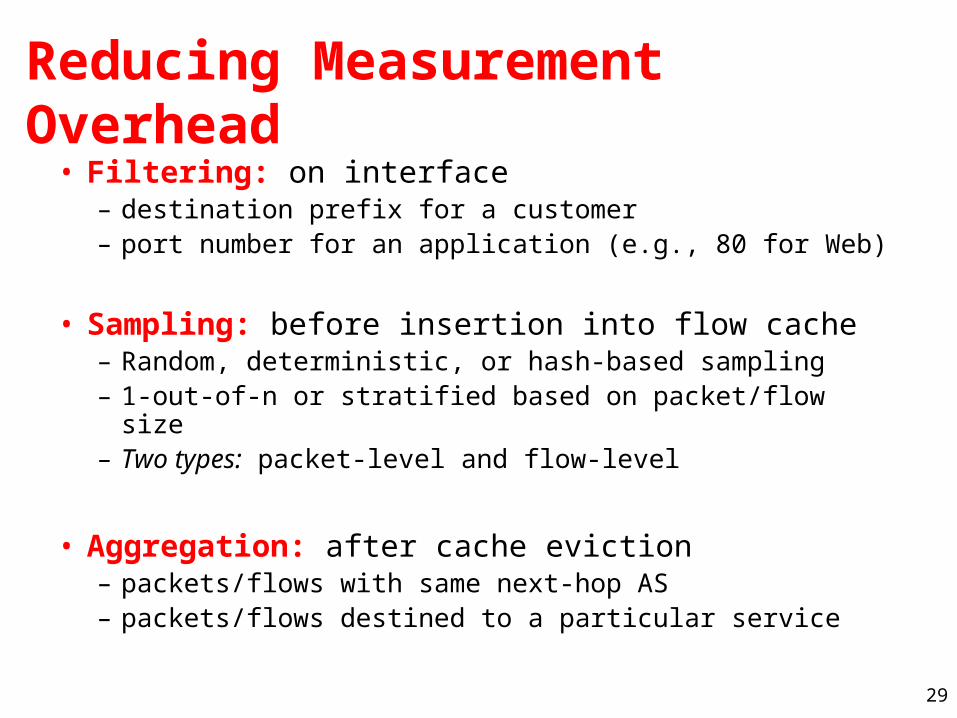
Reducing Measurement Overhead

• Filtering: on interface– destination prefix for a customer– port number for an application (e.g., 80 for Web)

• Sampling: before insertion into flow cache– Random, deterministic, or hash-based sampling– 1-out-of-n or stratified based on packet/flow size– Two types: packet-level and flow-level

• Aggregation: after cache eviction– packets/flows with same next-hop AS– packets/flows destined to a particular service

30

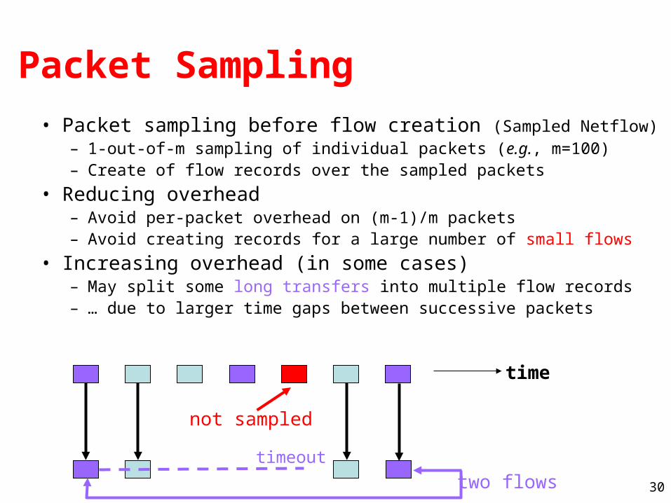
Packet Sampling

• Packet sampling before flow creation (Sampled Netflow)– 1-out-of-m sampling of individual packets (e.g., m=100)– Create of flow records over the sampled packets

• Reducing overhead– Avoid per-packet overhead on (m-1)/m packets– Avoid creating records for a large number of small flows

• Increasing overhead (in some cases)– May split some long transfers into multiple flow records – … due to larger time gaps between successive packets

time

not sampled

two flowstimeout

31

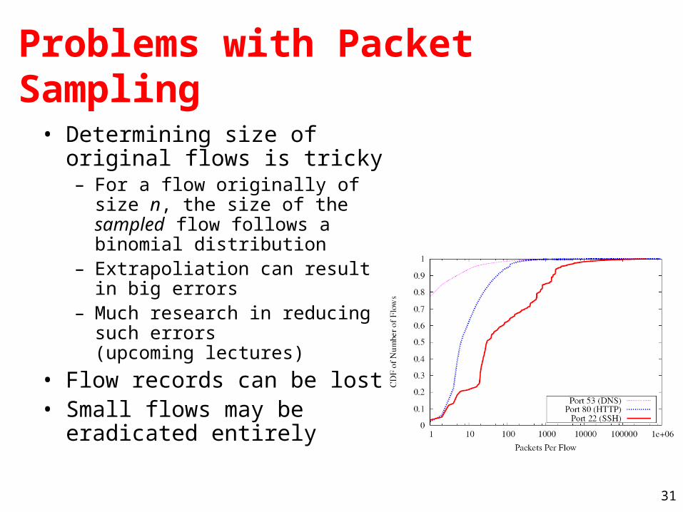
Problems with Packet Sampling

• Determining size of original flows is tricky– For a flow originally of size n, the

size of the sampled flow follows a binomial distribution

– Extrapoliation can result in big errors

– Much research in reducing such errors (upcoming lectures)

• Flow records can be lost• Small flows may be eradicated

entirely

32

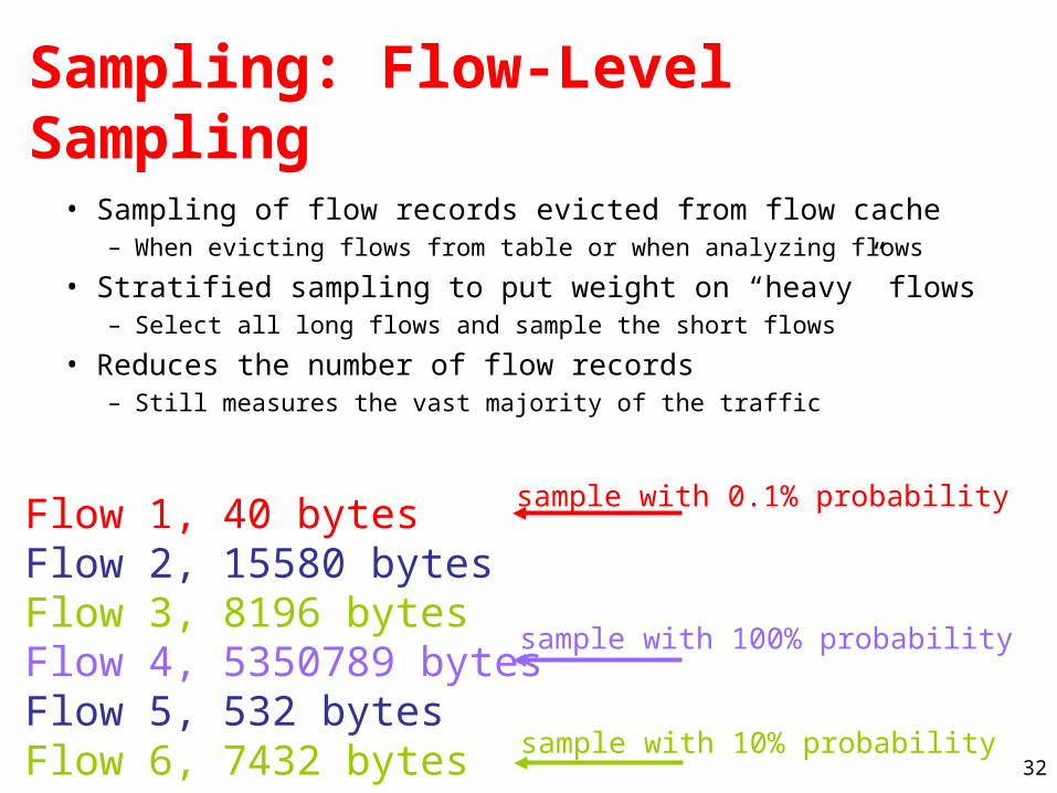
Sampling: Flow-Level Sampling

• Sampling of flow records evicted from flow cache– When evicting flows from table or when analyzing flows

• Stratified sampling to put weight on “heavy” flows– Select all long flows and sample the short flows

• Reduces the number of flow records – Still measures the vast majority of the traffic

Flow 1, 40 bytesFlow 2, 15580 bytesFlow 3, 8196 bytesFlow 4, 5350789 bytesFlow 5, 532 bytesFlow 6, 7432 bytes

sample with 100% probability

sample with 0.1% probability

sample with 10% probability

33

Accuracy Depends on Phenomenon

• Even naïve random sampling probably decent for capturing the existence of large flows

• Accurately measuring other features may require different approaches– Sizes of large flows – Distribution of flow sizes– Existence of small flows (coupon collection)– Size of small flows– Traffic “matrix”

34

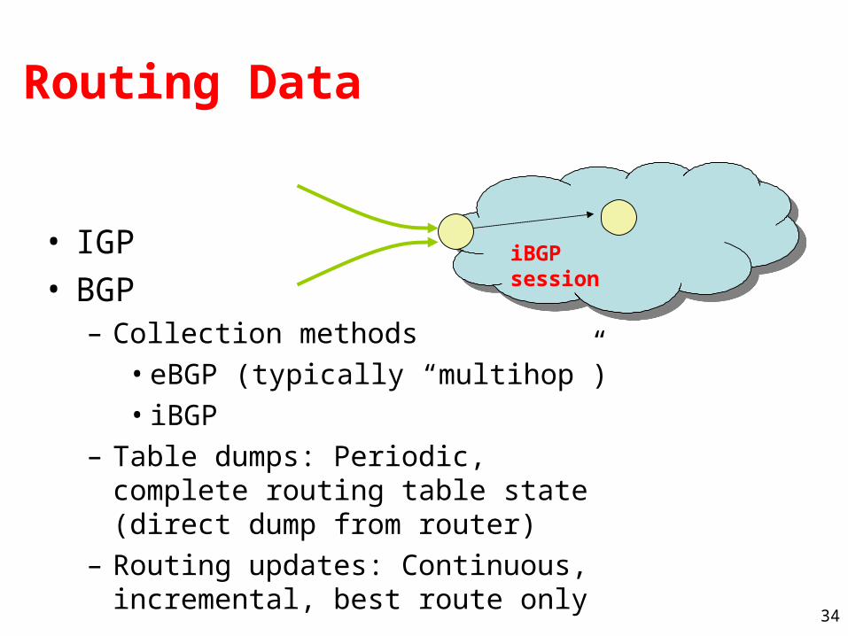
Routing Data

• IGP• BGP

– Collection methods• eBGP (typically “multihop”)• iBGP

– Table dumps: Periodic, complete routing table state (direct dump from router)

– Routing updates: Continuous, incremental, best route only

iBGP session

Evaluation Strategies and Platforms

36

Other Measurement Tools

• Scriptroute (http://www.scriptroute.org/)– Write new probing tools/techniques, etc.– More on PS 2

37

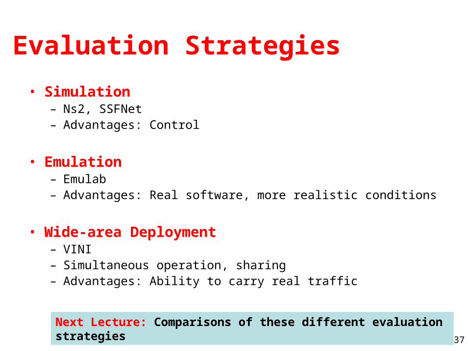
Evaluation Strategies

• Simulation– Ns2, SSFNet– Advantages: Control

• Emulation– Emulab– Advantages: Real software, more realistic conditions

• Wide-area Deployment– VINI– Simultaneous operation, sharing– Advantages: Ability to carry real traffic

Next Lecture: Comparisons of these different evaluation strategies

38

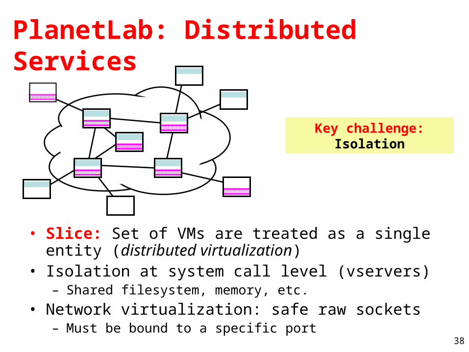
PlanetLab: Distributed Services

• Slice: Set of VMs are treated as a single entity (distributed virtualization)

• Isolation at system call level (vservers)– Shared filesystem, memory, etc.

• Network virtualization: safe raw sockets– Must be bound to a specific port

Key challenge: Isolation

39

Virtualization

• Advantages– Simultaneous access to shared physical resources

• Disadvantages– Requires scheduling– Not running on “raw” hardware. May not see similar

performance as the “real” network/system

40

PlanetLab for Network Measurement

• Nodes are largely at academic sites– Other alternatives: RON testbed (disadvantage:

difficult to run long running measurements)

• Repeatability of network experiments is tricky– Proportional sharing

• Minimum guarantees provided by limiting the number of outstanding shares

– Work-conserving CPU scheduler means experiment could get more resources if there is less contention

41

PlanetLab for Network Architecture

• New components must be virtualized– Interfaces– Links

• Support for forwarding traffic over virtual links

• Stock and custom routing software