Embed Size (px)
Citation preview

Traffic Management and Control
in Intelligent Vehicle Highway Systems
L.D. Baskar

.

Traffic Management and Control
in Intelligent Vehicle Highway Systems
Proefschrift
ter verkrijging van de graad van doctoraan de Technische Universiteit Delft,
op gezag van de Rector Magnificus prof. dr. ir. J.T. Fokkema,voorzitter van het College van Promoties,
in het openbaar te verdedigen op woensdag 18 november 2009 om 12.30 uurdoor Lakshmi Dhevi BASKAR,
master of science in computer science, Otto-von-Guericke Universität Magdeburg,geboren te Erode, Tamil Nadu, India.

Dit proefschrift is goedgekeurd door de promotoren:Prof.dr.ir. J. HellendoornProf.dr.ir. B. De Schutter
Samenstelling promotiecommissie:
Rector Magnificus voorzitterProf.dr.ir. J. Hellendoorn Technische Universiteit Delft, promotorProf.dr.ir. B. De Schutter Technische Universiteit Delft, promotorDr. Z. Papp TNO Science and Industry, DelftProf.dr.ir. S.P. Hoogendoorn Technische Universiteit DelftProf.dr. C. Witteveen Technische Universiteit DelftProf.dr.ir. B. van Arem Technische Universiteit DelftProf.Dr.-Ing. F. Busch Technische Universität München
The research described in this thesis was supported by the VIDI project “Multi-Agent Con-trol of Large-Scale Hybrid Systems” (DWV.6188) of the Dutch Technology FoundationSTW and the BSIK project “Transition to Sustainable Mobility (TRANSUMO)”
TRAIL Thesis Series T2009/12, the Netherlands TRAIL Research School
P.O. Box 50172600 GA Delft, The NetherlandsT: +31 (0) 15 278 6046T: +31 (0) 15 278 4333E: [email protected]
Published and distributed by: L.D. BaskarE-mail: [email protected]
ISBN 978-90-5584-120-2
Keywords: intelligent vehicle highway systems, intelligent transportation systems, intelli-gent vehicles, model predictive control
Copyright c© 2009 by L.D. Baskar
All rights reserved. No part of the material protected by this copyright notice may be re-produced or utilized in any form or by any means, electronic or mechanical, including pho-tocopying, recording or by any information storage and retrieval system, without writtenpermission of the author.
Printed in the Netherlands

Preface
Hurray, I made it! This is first impression I got when I completed my thesis writing. Thiswas not an easy task for a person who comes from a different educational background. MyPhD research involved learning of new technical skills as well discovering myself. I hadthis research opportunity, which many people as deserving as me did not get. So I workedhard to achieve it. I owe a lot of thanks to many people who made this research career, firstpossible and also an experience to hold on.
It is usual to say that I thank my supervisors Hans and Bart for believing in me and fortheir support, guidance, positively told criticisms, and reviews provided during my PhD.But for me, this is not just meant to be in words. Apart from motivating me, stream liningthe ideas to carry out the research in a proper direction, I thank Hans for his simplicity andhis easily approachable character. Hans never forgets to appreciate the person for what theyhave done, for instance, even if it is a presentation or after every thesis chapter is completed.Hans makes a point to ask how my research is going as well as to ask how my vacation was.
I am really grateful to my daily supervisor Bart for his persistent support during bothbad and good times of my profession and in my personal life. Bart, I thank you for makingme comfortable by stating that the research is a team work. Though he is occupied thewhole day, Bart has always time to answer my doubts, even at late nights. All I can say is,Bart as a supervisor and as an understanding human gave a helping hand in all professionalways to encourage me to do my research. He drops in my office just to ask me if I am in arelaxed mind to carry out the research.
I thank my PhD committee members Dr. Zoltan Papp, Prof. Bart van Arem, Prof. SergeHoogendoorn, Prof. Cees Witteveen, Prof. Fritz Busch, Prof. Hans Hellendoorn and Prof.Bart De Schutter for their valuable time and suggestions provided to improvise my thesis.
I also thank the students Mernout Burger and Berend de Graaf, whom I supervisedduring their final work. Their work provided a substantial contribution to this thesis.
My special thanks to my beloved parents Baskaran and Shanthi Baskaran, my brotherSantosh, and my best, adorable friends Prasanna in Brussels, and Mani and Shanthi Bas-karan in India. Other important personalities are Mrs. Arsha Timmermans, Mrs. AlettaWubben, and Mrs. Tineke Holkema. I greatly appreciate them for their interests in makingme realise the need for a balance in my research and personal life. I take this opportunity tothank my all DCSC colleagues and my friends. In particular, I wish to thank Alina, Amol,Andreas, Dang, Jianfei, Monique, Navin, Ronald, Rudy, Samira, Solomon, Shu, Mrs. Kittyand Mrs. Ellen from DCSC and Mrs. Conchita from TRAIL, and Gayatri, Sampath, Rohini,Raghu, Joe and Abhijeet in Delft.
L.D. Baskar, Delft, November 2009.
v

vi

Contents
Preface v
1 Introduction 1
1.1 Motivation and goals . . . . . . . . . . . . . . . . . . . . . . . . . . . . . 21.2 General overview of the thesis . . . . . . . . . . . . . . . . . . . . . . . . 6
1.2.1 Outline of the thesis . . . . . . . . . . . . . . . . . . . . . . . . . 61.2.2 Main contributions . . . . . . . . . . . . . . . . . . . . . . . . . . 81.2.3 Road map . . . . . . . . . . . . . . . . . . . . . . . . . . . . . . . 9
2 Traffic Management and Intelligent Vehicle Highway Systems: State-of-the-
Art 11
2.1 Introduction . . . . . . . . . . . . . . . . . . . . . . . . . . . . . . . . . . 112.2 Control design methods . . . . . . . . . . . . . . . . . . . . . . . . . . . . 13
2.2.1 Static feedback control . . . . . . . . . . . . . . . . . . . . . . . . 142.2.2 Optimal control and model predictive control . . . . . . . . . . . . 162.2.3 Artificial intelligence techniques . . . . . . . . . . . . . . . . . . . 192.2.4 Comparison . . . . . . . . . . . . . . . . . . . . . . . . . . . . . . 22
2.3 Intelligent vehicles and traffic control . . . . . . . . . . . . . . . . . . . . 242.3.1 Intelligent vehicles . . . . . . . . . . . . . . . . . . . . . . . . . . 242.3.2 IV-based traffic management . . . . . . . . . . . . . . . . . . . . . 252.3.3 IV-based control measures . . . . . . . . . . . . . . . . . . . . . . 26
2.4 Control frameworks and architectures for IVHS . . . . . . . . . . . . . . . 272.4.1 PATH framework . . . . . . . . . . . . . . . . . . . . . . . . . . . 272.4.2 Dolphin framework . . . . . . . . . . . . . . . . . . . . . . . . . . 292.4.3 Auto21 CDS framework . . . . . . . . . . . . . . . . . . . . . . . 302.4.4 CVIS . . . . . . . . . . . . . . . . . . . . . . . . . . . . . . . . . 322.4.5 SafeSpot . . . . . . . . . . . . . . . . . . . . . . . . . . . . . . . 322.4.6 PReVENT . . . . . . . . . . . . . . . . . . . . . . . . . . . . . . 33
2.5 Comparison of the IVHS frameworks . . . . . . . . . . . . . . . . . . . . 342.6 Outlook . . . . . . . . . . . . . . . . . . . . . . . . . . . . . . . . . . . . 36
2.6.1 Application to IVHS . . . . . . . . . . . . . . . . . . . . . . . . . 362.6.2 Challenges and open issues . . . . . . . . . . . . . . . . . . . . . . 37
2.7 Summary . . . . . . . . . . . . . . . . . . . . . . . . . . . . . . . . . . . 39
vii

viii Contents
3 A New Traffic Management Framework for IVHS 41
3.1 Introduction . . . . . . . . . . . . . . . . . . . . . . . . . . . . . . . . . . 413.2 IV-based control framework . . . . . . . . . . . . . . . . . . . . . . . . . 41
3.2.1 Proposed control framework . . . . . . . . . . . . . . . . . . . . . 423.3 Main improvements and extensions . . . . . . . . . . . . . . . . . . . . . 43
3.3.1 Integrated in-vehicle and roadside control measures . . . . . . . . . 443.4 Contributions of our approach . . . . . . . . . . . . . . . . . . . . . . . . 453.5 Open problems . . . . . . . . . . . . . . . . . . . . . . . . . . . . . . . . 453.6 Summary . . . . . . . . . . . . . . . . . . . . . . . . . . . . . . . . . . . 46
4 Roadside Controller 47
4.1 Introduction . . . . . . . . . . . . . . . . . . . . . . . . . . . . . . . . . . 474.2 A hierarchical framework for IV-based traffic management . . . . . . . . . 484.3 Model Predictive Control (MPC) . . . . . . . . . . . . . . . . . . . . . . . 504.4 MPC for IVHS . . . . . . . . . . . . . . . . . . . . . . . . . . . . . . . . 51
4.4.1 States and control inputs . . . . . . . . . . . . . . . . . . . . . . . 514.4.2 Performance criterion and constraints . . . . . . . . . . . . . . . . 514.4.3 Optimisation methods . . . . . . . . . . . . . . . . . . . . . . . . 524.4.4 Prediction models for IVHS . . . . . . . . . . . . . . . . . . . . . 524.4.5 Platoon-based prediction model . . . . . . . . . . . . . . . . . . . 55
4.5 Case study . . . . . . . . . . . . . . . . . . . . . . . . . . . . . . . . . . . 564.5.1 Set-up . . . . . . . . . . . . . . . . . . . . . . . . . . . . . . . . . 564.5.2 Scenario . . . . . . . . . . . . . . . . . . . . . . . . . . . . . . . . 574.5.3 Models . . . . . . . . . . . . . . . . . . . . . . . . . . . . . . . . 574.5.4 Control problem . . . . . . . . . . . . . . . . . . . . . . . . . . . 584.5.5 Results and analysis . . . . . . . . . . . . . . . . . . . . . . . . . 61
4.6 Summary . . . . . . . . . . . . . . . . . . . . . . . . . . . . . . . . . . . 67
5 Area Controller 69
5.1 Introduction . . . . . . . . . . . . . . . . . . . . . . . . . . . . . . . . . . 695.2 Intelligent vehicle highway systems (IVHS) . . . . . . . . . . . . . . . . . 715.3 Optimal route choice control in IVHS using mixed-integer linear programming 72
5.3.1 Approach . . . . . . . . . . . . . . . . . . . . . . . . . . . . . . . 725.3.2 Set-up . . . . . . . . . . . . . . . . . . . . . . . . . . . . . . . . . 735.3.3 Static case with sufficient network capacity . . . . . . . . . . . . . 745.3.4 Static case with queues at the boundaries of the network only . . . . 745.3.5 Dynamic case with queues at the boundaries of the network only . . 755.3.6 Dynamic case with queues inside the network . . . . . . . . . . . . 775.3.7 Approximation based on mixed-integer linear programming . . . . 795.3.8 Case study . . . . . . . . . . . . . . . . . . . . . . . . . . . . . . 81
5.4 Optimal routing for IVHS using a macroscopic traffic flow model . . . . . . 835.4.1 Macroscopic traffic flow characteristics . . . . . . . . . . . . . . . 845.4.2 Macroscopic traffic flow for IVs . . . . . . . . . . . . . . . . . . . 855.4.3 A METANET-like macroscopic model for IVs . . . . . . . . . . . 865.4.4 Model predictive route choice control . . . . . . . . . . . . . . . . 925.4.5 Case study . . . . . . . . . . . . . . . . . . . . . . . . . . . . . . 93

Contents ix
5.5 Interface between area and roadside controllers . . . . . . . . . . . . . . . 955.6 Summary . . . . . . . . . . . . . . . . . . . . . . . . . . . . . . . . . . . 96
6 Traffic Management with Semi-Autonomous Intelligent Vehicles 99
6.1 Introduction . . . . . . . . . . . . . . . . . . . . . . . . . . . . . . . . . . 996.2 Preliminaries . . . . . . . . . . . . . . . . . . . . . . . . . . . . . . . . . 100
6.2.1 Model Predictive Control (MPC) . . . . . . . . . . . . . . . . . . . 1006.2.2 In-vehicle measures . . . . . . . . . . . . . . . . . . . . . . . . . 101
6.3 MPC for semi-autonomous traffic . . . . . . . . . . . . . . . . . . . . . . 1016.3.1 Prediction model . . . . . . . . . . . . . . . . . . . . . . . . . . . 1016.3.2 Performance criteria and constraints . . . . . . . . . . . . . . . . . 104
6.4 Simulation model - Paramics . . . . . . . . . . . . . . . . . . . . . . . . . 1046.5 Coupling Paramics and Matlab . . . . . . . . . . . . . . . . . . . . . . . . 107
6.5.1 Interface plugin . . . . . . . . . . . . . . . . . . . . . . . . . . . . 1076.5.2 ISA plugin . . . . . . . . . . . . . . . . . . . . . . . . . . . . . . 109
6.6 Case study . . . . . . . . . . . . . . . . . . . . . . . . . . . . . . . . . . . 1116.6.1 Set-up . . . . . . . . . . . . . . . . . . . . . . . . . . . . . . . . . 1116.6.2 Scenario . . . . . . . . . . . . . . . . . . . . . . . . . . . . . . . . 1126.6.3 Models . . . . . . . . . . . . . . . . . . . . . . . . . . . . . . . . 1136.6.4 Control problem . . . . . . . . . . . . . . . . . . . . . . . . . . . 1166.6.5 Results and analysis . . . . . . . . . . . . . . . . . . . . . . . . . 116
6.7 Summary . . . . . . . . . . . . . . . . . . . . . . . . . . . . . . . . . . . 122
7 Conclusions and Recommendations 125
7.1 Main contributions . . . . . . . . . . . . . . . . . . . . . . . . . . . . . . 1257.2 Conclusions . . . . . . . . . . . . . . . . . . . . . . . . . . . . . . . . . . 126
7.2.1 Main conclusions . . . . . . . . . . . . . . . . . . . . . . . . . . . 1267.2.2 Conclusions per chapter . . . . . . . . . . . . . . . . . . . . . . . 126
7.3 Open problems and recommendations for future research . . . . . . . . . . 128
Bibliography 133
Glossary 145
Samenvatting 149
Summary 151
Curriculum vitae 153
TRAIL Thesis Series 155

x Contents

Chapter 1
Introduction
Most of the problems faced by today’s traffic networks are caused by the ever-increasingusage of the traffic system. Traffic congestion is considered to be one of the prominentissues that needs attention. Traffic control and management experts and policy makers havecome up with many possible solutions to solve the traffic congestion problem. Some ofthese solutions focused either on increasing the number of roads or lanes to cope with thedemand, or on limiting the traffic demand by levying tolls and raising taxes for using thesystem. Also, due to political concerns and feasibility constraints, both of these optionsdid not offer a promising solution. Another solution is to use the current system in a moreefficient way. This option offers high benefits and potential both on the short term and thelong term. This approach is worked out in this thesis, with a particular focus on the longterm.
In terms of conventional traffic control approaches, efficient utilisation is made possibleby controlling and managing the roadside infrastructure intelligently, which in turn can im-prove the traffic performance. Currently, this intelligence is introduced in the traffic systemsby means of roadside based measures and control handles such as dynamic route guidancepanels, ramp metering systems, dynamic speed limits, and also by means of infrastructureequipment such as sensors and actuators. Meanwhile, the other important element in thetraffic system — i.e., the vehicles — have become much more intelligent. By this intelli-gence, we mean that the vehicles are equipped with a number of on-board sensors that helpin gathering information such as their position and speed, and with many fast devices thatprocess and present the obtained information in a meaningful and usable form [21]. Thesetechniques can then assist or control the driver actions to sustain a safe and better drivingoperation.
The traffic management industry thus recognised the importance of the technologiesfrom the fields of telecommunication, control, and information sciences, and decided to putthem to use along with the current roadside infrastructure and equipment. This resulted in anIntelligent Vehicle Highway System (IVHS) – a basic medium to distribute the intelligencebetween vehicles and the roadside infrastructure, and to improve the traffic performancein a reliable and efficient manner. This performance can be expressed in terms of safety,throughput, travel time, fuel emissions, etc.
An IVHS is not a newly developed system, but a next level of traffic control and man-
1

2 1 Introduction
agement approach that efficiently combines and coordinates systems in both the roadsideinfrastructure and in the vehicles. In general, IVHS includes roadside-based activities suchas controlling and managing the traffic network, and vehicle-based activities such as con-trolling and steering individual vehicles.
Intelligent Vehicles (IVs) in the IVHS can sense the driving environment using sensorsand can provide assistance to the driver (via warnings or advisories) or can take completecontrol of the vehicle itself to achieve an efficient vehicle operation. These vehicle con-trol systems can thus shift driving tasks such as steering, braking, and throttle control fromdrivers to the on-board controllers in the vehicles. This complete control of driving tasksleads to an automated driving, which in turn allows the vehicles’ activities to be fully con-trolled by the traffic control and management systems. Such IVs with complete automationalso reduce the negative effects of driver delays and errors.
This fully automated handling of IVs allows the vehicles to be arranged in a closelyspaced group called platoons. In a platoon, the first vehicle is called a leader and the re-maining are followers. In this approach, the vehicles travel as platoons on the highways withhigh speeds. For safety reasons, larger distances are maintained between the platoons. Thevehicles inside the platoon maintain a small safety distance to avoid crashes between them.By travelling at a high speed and with short distances between vehicles, more vehicles canbe accommodated on the network, which in turn also yields an improvement in the trafficflow. Although the platooning approach offers a significant improvement in the traffic flow,the implementation of this approach in practice was considered to be impossible in the1990s. Due to the increasing penetration of advanced in-vehicle technologies in the marketand the availability of faster computers, we believe that the difficulties regarding safety, ac-ceptance of automation, and legal issues can be handled in a much better way in course oftime, so that ultimately IVHS can actually be implemented and widely deployed in practice.
Till now, much attention has been given to the development of advanced vehicle controlsystems and to conventional traffic control approaches. Although IVHS contain both road-side infrastructure and IVs, the link that connects these elements has obtained less attention.In this thesis we will address this issue and bridge this gap between the roadside infra-structure and the automated IVs by developing a framework and approach for IVHS-basedtraffic management and control that integrates roadside-based and IV-based traffic controlmeasures.
1.1 Motivation and goals
In this thesis, we will investigate the possibilities to implement a next generation trafficcontrol and management approach. This approach shifts away from a global roadside trafficmanagement to a more vehicle-based and user-specific network-based traffic management.The primary areas of interest that served as a basis to our research involve the followingelements:
• IV-based traffic control measures,
• Control structure,
• Control methodology.
Based on this discussion, we will then formulate the objectives of this thesis.

1.1 Motivation and goals 3
IV-based traffic control measures
Currently applied traffic control methods influence the traffic system solely using roadside-based control tools. Although these conventional approaches are striving to improve theperformance of traffic systems, there is still plenty of room for new contributions.
On the other hand, a slow but steady deployment of IVs into the market has shown theiracceptance by the users and their effectiveness in assisting the driving operations in a moresafe and robust manner [22, 111, 151]. Some functionalities that currently exist and that areavailable on the market are Adaptive Cruise Control (ACC) and dynamic route guidance.As more and more vehicle support technologies that are intelligent enough are introducedinto the current system, we believe that IV techniques — when chosen and utilised properlyalong with the conventional traffic control measures such as dynamic speed limits, routeguidance, ramp metering, lane closures, etc — have the potential to bring significant im-provements to the existing traffic system.
Since we opt to use the IVHS approach, we will work with automated IVs in com-bination with the platooning approach. Full automation of driving tasks in platoons canenhance the performance of the traffic system. This envisioned improvement in the systemperformance motivated us to use IV-based control handles and measures for traffic man-agement and control purposes. These IV-based control measures will then act as a controlinterface between the roadside infrastructure and the platoons of IVs. The roadside trafficcontrollers will use IV control measures such as route guidance systems, Intelligent SpeedAdaptation (ISA) along with the conventional traffic control measures to control platoonsof IVs. In particular, every platoon leader is controlled by the on-board controller andthe rest of the vehicles in platoons follow their respective leaders. By this approach, theintelligence is distributed between roadside traffic control measures and in-vehicle techno-logies, and is integrated to provide a roadside-vehicle-specific management rather than justa roadside-infrastructure management. Also, the IV measures should be selected such thattheir functionality does not counteract with each other and also with the existing conven-tional roadside control measures. Hence, the new set of all possible control measures shouldbe coordinated so as to serve the same objective.
Control structure
Having discussed the use of IV-based measures for traffic control and management pur-poses, the next question that arises is how to develop a control methodology that can handleand coordinate these control measures, and that can be implemented in a large-scale trafficnetwork. To obtain a tractable methodology, we should first select an appropriate controlstructure to tackle a large-scale traffic problem [4]. In general, appropriateness of any con-trol structure for a large-scale system can be analysed in terms of scalability, computationalcomplexity, communication overhead, and etc. Scalability refers to the ability of the struc-ture to handle the growing size of the problem both in space and in time. The computationalcomplexity is analysed through the amount of memory and time required to solve the prob-lem. Communication overhead is determined by the bandwidth requirements and by thetime involved in communications rather than in finding a solution for the problem. We willclassify the most commonly used control structures as follows:
• Centralised,

4 1 Introduction
agent 1
agent 2
supervisor 1 supervisor 2
high−level supervisor
agent 4
agent 3
agent 5
Figure 1.1: General representation of a hierarchical, distributed control structure
• Distributed,
• Hierarchical
Up to now, most control methods are based on a centralised control paradigm. However,in practice, centralised control of large-scale traffic systems is often infeasible due to lackof scalability, computational complexity, and communication overhead. For these reasons,we prefer a distributed approach, which can overcome the shortcomings of the centralisedapproach [52, 134]. In a distributed approach, the control problem is divided into manysubproblems, with each subproblem being managed by a local controller. The local con-troller is responsible for the problems that occur in its area and it has the complete freedomto choose the ways to solve the problems. Finally, all these subproblem solutions can besummed up to yield the global solution. An additional advantage of a distributed controlapproach us that it results in a controlled system that is more robust to system failures.
To control a large-scale traffic system, a distributed approach with hierarchical or multi-layered structure can make the task of controlling manageable and can deal with the increas-ing complexity of the system by adding layers, without changing the complete structure.The key factors such as coordination and system tractability, offered by the hierarchical anddistributed control structure motivated us to use this approach for controlling a large-scaletraffic system. Such an approach is based on the principle of “divide and conquer” and al-lows us to split the task of controlling the network into several subproblems (either at thesame level (for a distributed approach) or at several levels (for a hierarchical approach).Thus, by deploying this structure, the activities of the local traffic centres can be coordin-ated by a supervisory traffic centre and this will result in managing the traffic system in afeasible manner. Such a multi-level control structure with local control agents at the lowestlevel, and one or more higher supervisory control level, is shown in Figure 1.1.
For illustration purposes, let us apply these approaches to a communication network.Consider a client-server system for watching online movies on the Internet based on a cent-ralised design. As the number of users accessing the web site increases, the server getsoverloaded, faces buffering problems, and becomes too busy for further access. Thus the

1.1 Motivation and goals 5
centralised system cannot serve the users when the demand is large. To solve this, onecan make use of peer-to-peer networks, and this network can be viewed as a distributedsystem. This approach provides a reliable operation even when the number of users thatsimultaneously access the system increases, as the resource can be found in various peerswithout relying on a centralised server. In a distributed approach, the failures that occur inone subsystem can be dealt with without causing much problems to the other subsystems inthe network that are coupled to the faulty subsystem. Hence, a single point of failure in thesystem is avoided in the distributed system.
While applying these approaches to control and to manage a large-scale traffic system,a centralised approach will face similar problems as in the client-server system and mightproduce infeasible solutions. Hence, we prefer to use a distributed control approach. Thisapproach will then have local traffic control centres operating at main cities and these centresare responsible for controlling the traffic activities in their respective areas. However, whena local controller has an unresolved problem, or two traffic control centres have to sharethe same resources, then the involved control centres should not affect other neighbourswith their adverse effects. In these cases, coordination plays a key role to obtain a peacefuland fruitful agreement among the neighbours, and this process can be carried out by asupervisory controller through communications and negotiations.
Control methodology
Now moving on to the actual control methodology, the control design should be flexible andadaptable to dynamic changes in the demands and working conditions, and in the structureof the system. The changes in the system behaviour can be caused by unexpected eventssuch as incidents or accidents on the highways. Usually, the demand and traffic conditionsare time-variant and characterised by a high degree of uncertainty. Hence, static or fixedcontrol strategies usually do not suit our purpose, and an adaptable, robust, and feedback-based control method is required. In traffic control, the process of feedback is considered asan essential property to handle unknown disturbances that act on the system in time and toreduce their negative effects.
Due to platoon-specific management, the possible combinations of control measuresthat a roadside traffic controller has to consider can be an integer or a real-valued problemor a combination of both. These combinations can make the traffic problem much morecomplex. In general, the control method should be able to handle this complexity, to dealwith multiple objective functions, and to satisfy those constraints that are imposed on thesystem while determining optimal solutions for the problem. The resulting multi-objectiveconstrained control or optimisation problem should result in optimal values for and coordin-ation of the selected control measures.
All these requirements lead us to choose a control technique that is advanced, robust,adaptive, predictive, and model-based, and that can operate in real-time. Our work is in-spired by the work of Papageorgiou and his co-workers [90, 93, 104] and of Bellemans andHegyi [17, 18, 64, 66, 67], where a model-based approach such as Model-based Predict-ive Control (MPC) is used for traffic control and management. The traffic controller usesMPC for predicting the future behaviour of the system due to external inputs and demands,and for predicting the effects of various control measures on the system. The underly-ing concept of the MPC controller is based on on-line optimisation and uses an explicit

6 1 Introduction
prediction model to obtain the optimal actions for the control measures subject to systemdynamics and constraints. However, this technique also comes with its own advantages anddisadvantages: The advantage is that the MPC is a feedback control algorithm which canhandle constrained, complex dynamical systems. However, since it is a model-based ap-proach, certain criteria on the model need to be satisfied. The model that will be used forprediction purposes should be fast, does not need to represent fine details of the system, butshould reproduce the traffic evolution with a sufficient degree of accuracy. We will discussthese issues in more detail in the next chapters.
Goals
The goals of this thesis are to design a framework to control large-scale traffic networksusing a multi-level control structure and to determine a tractable control design methodologyfor use within this framework. In particular, our framework will be designed to suit a variantof the IVHS setup. The IVHS set-up we consider in addition uses the monitoring and controlcapabilities offered by automated IVs that support the platooning approach and combinesthem with conventional traffic control measures. Once the framework is designed, we willdevelop a structured and tractable design methodology for robust control of the IVHS.
Our focus will be on traffic control and management strategies for the IVHS, with spe-cial attention at the roadside infrastructure. We are mainly interested in developing waysto design an appropriate distributed, hierarchical control structure for our IVHS, to determ-ine control design methods that can integrate the IV-based techniques along with existingtraffic control measures, to adapt the currently used control measures to fit the new IVHSframework, and also to make a selection of control methods that are suitable to be appliedat different levels of control. A detailed analysis of the performance and complexity of themethods and of the resulting controllers has to be made using relevant case studies.
Furthermore, we have made some assumptions in our work. We will not deal with legaland user acceptance issues of the new system, and neither with the development of protocolsfor communication and coordination purposes. We also assume that the automated IVsand the roadside infrastructure are equipped with the necessary communication and controlcomponents to provide and respond to the roadside-IV control measures. Also, we assumethat the vehicle and platoon controllers to be present and designed according to literature[77, 139, 147].
1.2 General overview of the thesis
In this section, we give an overview of the topics that will be dealt with in each chapter ofthis thesis. In particular, Section 1.2.1 provides a brief summary of the contents of eachchapter, and briefly discusses the contributions made by this thesis to the state-of-the-art.Next, the road map in Section 1.2.3 guides the readers to understand the structure of thethesis.
1.2.1 Outline of the thesis
In this thesis, we propose a multi-level framework for IVHS-based traffic management andcontrol. In particular, we will implement IV-based control design methods at different levels

1.2 General overview of the thesis 7
of the roadside infrastructure in our new IVHS-framework and analyse their potential con-tribution to improve the performance of the system. This thesis is organised as follows:
• Chapter 2 deals with two main streams of topics. First, we give an overview ofcontrol design methodologies that are most often used to control the traffic on high-ways. Most of the control methods that have been presented in the literature dealwith vehicles that are driven by humans. On the basis of this survey, we make a com-parative analysis of these methodologies and also sketch how these methods couldfit in an IVHS-based traffic control framework. Next, we discuss intelligent vehiclesand describe how the IV-based control measures and handles can be used to improvethe traffic flow. Subsequently, we discuss various existing traffic management ar-chitectures for IVHS such as PATH, Dolphin, Auto21 CDS, CVIS, SafeSpot, andPReVENT. As a result of the survey on IVs and IVHS-frameworks, we provide aqualitative comparison of these frameworks based on their strong and weak points.The last section of the chapter discusses some open issues regarding IVHS as well asthe practical challenges in their deployment.
• Subsequently in Chapter 3, we introduce a new framework for IVHS that meets ourgoals stated in Section 1.1 and that considers and combines the strong points of otherexisting IVHS-based control architectures discussed in Chapter 2. Our new frame-work is capable of distributing the intelligence between vehicles and roadside infra-structure, and integrates IV-based measures and the conventional roadside traffic con-trol measures. We describe the main features of our new multi-level framework andalso sketch the contributions that our approach can provide for the improvement oftraffic performance. Our framework also allows vehicle-vehicle and vehicle-roadsidecommunications. Due to the legal and practical acceptance of this system and imple-mentation issues that may be involved, we can say that the newly proposed frame-work, in general, is a research result aimed at the future.
• In Chapter 4, we specifically focus on the roadside controller, which integrates theidentified IV-based control measures and conventional traffic control measures, andwhich assigns traffic control actions based on the platooning approach. The imple-mentation of this controller is the first and crucial step towards the deployment of ourframework. The actual control strategy that will be used by the controller is the MPCapproach. Each roadside controller will control a stretch of a highway in the networkand it will provide optimal control commands such as dynamic speed limits, lane al-locations for each platoon on the highway stretch, and release times for the platoonsat on-ramps. These commands are then realised by the platoons of automated IVs onthe highways by means of Intelligent Speed Adaptation (ISA), Adaptive Cruise Con-trol (ACC), and other necessary sensors and communication protocols. To analysethe potential benefits of the new framework, we compare the proposed approach bothfor traffic scenarios with human driven IVs and with IV-based platoons.
• Next, we move up one level in the hierarchical IVHS-based traffic control framework .In Chapter 5, we deal with the area controller, which controls a set of interconnectedhighways and which coordinates the activities of various roadside controllers in itsarea. The area controller is responsible for assigning optimal routes to the platoonsin the IVHS. Since in general the optimal routing problem results in a mixed-integer

8 1 Introduction
problem, which is hard to solve, we propose two approximate models (one solelybased on flows and queue lengths, and one that is an adaptation of METANET, amacroscopic traffic flow model for human drivers, to the case of platoons of intelligentvehicles). This results in simplified but fast simulation models that — when used foroptimal routing — yield mixed-integer linear or nonlinear real-valued optimisationproblems, for both of which efficient solvers exist.
• Chapter 6 considers an intermediate situation between the current conventionaltraffic management and system and the fully automated IVHS-based traffic manage-ment system of the future. In this chapter, we primarily investigate the possibilityof using semi-autonomous vehicles with advanced in-car systems for traffic control.For illustrating such a system, we consider a traffic system with vehicles that areequipped with fully autonomous ACC and advisory ISA. However, in contrast to thesystem considered in Chapters 3, 4, and 5, these vehicles do not travel in platoons.In this set-up the roadside controller calculates the dynamic speed limits and issuesthese limits using the speed limit display panels. We use a traffic simulation softwarepackage PARAMICS to represent the current traffic system, and we develop plug-ins to program the behaviour of the partially automated vehicles and their react tothe control measures. Matlab is chosen as the software environment to implementthe roadside controller. Since there is no existing interface between the two softwareprograms, we create a plug-in to connect Matlab and PARAMICS. We then considervarious scenarios in which we investigate and compare the effect of control on a trafficsystem driven by humans only and on a system with semi-automated IVs only.
• Finally, Chapter 7 summarises the main contributions of this thesis, followed bysome suggestions for future research.
Some of the material included in this thesis has already been published. In particular,Chapter 3 is based on [9, 10, 16], Chapter 4 is based on [11–15], and Chapter 6 is based onthe MSc thesis of Mernout Burger [29].
1.2.2 Main contributions
The contributions of this thesis to the state-of-the-art are:
• The study and analysis of the existing IVHS frameworks. Using a general structureof the IVHS traffic system, and based on the comparative analysis of the controlapproaches, we also suggest which control methodologies can be used at differentlevels of the framework.
• The development of a new multi-level IVHS framework that distributes the intelli-gence between roadside and platoons of automated IVs and that uses IV-based controlmeasures for controlling and managing the traffic system.
• The development of a control approach based on model-based predictive control thatcan be used by the roadside and area controllers and that allows to integrate andcoordinate various IV-based and roadside control measures such as ramp metering,dynamic speed limits, route guidance, etc.

1.2 General overview of the thesis 9
Recommendations7 − Conclusions
independent chapters
2 − State−of−the−art
1 − Introduction
3 − Proposed framework
controller4 − Roadside
ROADSIDE CONTROL
IVH
S
controller5 − Area
management with6 − Traffic
semi−autonomous IVs
*
*
*
*
Figure 1.2: A road map for the chapters
1.2.3 Road map
Figure 1.2 illustrates the organisation and the relations between the chapters of the thesisand also represents the way in which the chapters can be read. Some of the chapters ofthe thesis, viz. Chapters 4, 5, and 6 are written in such a way that the reader can read andunderstand that chapter independent of other chapters. These chapters are self-containedin the sense that they briefly recapitulate all the material of the preceding chapters that isnecessary to understand the contents of that particular chapter.
Before starting to read the thesis, we recommend the reader to have a first glance at thebasic structure of the thesis. The chapters can be read by following the flowchart shownin Figure 1.2. Chapter 1 gives a general introduction to the topics dealt in this thesis andputs emphasis on the research problem and goals. In Chapter 2 we discuss the state-of-the-art of the conventional control methodologies and the control architectures, particularly forIVHS-based traffic management. We suggest the reader to go through Chapter 3, as thischapter introduces our newly proposed IV-based framework and gives a description of con-trol responsibilities assigned at each level of the proposed framework. The self-containedChapters 4 and 5 also briefly summarise our newly proposed IVHS-framework and mainlyfocus on issues related to implementation of the control approaches at the roadside control-ler and area controller respectively. Chapter 6 is a different genre compared to Chapters 4

10 1 Introduction
and 5, as this chapter shows the possibility of implementing IV systems in the current trafficsystem. Chapter 7 summarises the contributions of this thesis and gives directions for futureresearch.

Chapter 2
Traffic Management and
Intelligent Vehicle Highway
Systems: State-of-the-Art
Traffic congestion in highway networks is one of the main issues to be addressed by today’straffic management schemes. Automation combined with the increasing market penetra-tion of on-line communication, navigation, and advanced driver assistance systems willultimately result in intelligent vehicle highway systems (IVHS) that distribute intelligencebetween roadside infrastructure and vehicles and that — in particular on the longer term —are one of the most promising solutions to the traffic congestion problem. In this chapter,we present a survey on traffic management and control frameworks for IVHS. First, we givea short overview of the main currently used traffic control methods for freeways. Next, wediscuss IVHS-based traffic control measures. Then, various traffic management architec-tures for IVHS such as PATH, Dolphin, Auto21 CDS, etc. are discussed and a comparisonof the various frameworks is presented. Finally, we sketch how existing traffic control meth-odologies could fit in an IVHS-based traffic control set-up.
2.1 Introduction
Due to the ever-increasing traffic demand, modern societies with well-planned road man-agement systems, and sufficient infrastructures for transportation still face the problem oftraffic congestion. This results in loss of travel time, and huge societal and economic costs.Constructing new roads could be one of the solutions for handling the traffic congestionproblem, but it is often less feasible due to political and environmental concerns. An altern-ative would be to make more efficient use of the existing infrastructure. In this chapter, wewill consider the latter approach with a special focus on freeway traffic management andcontrol.
Traffic management and control approaches are used to control the traffic flows and toprevent or reduce traffic jams, or more generally to improve the performance of the trafficsystem. Possible performance measures in this context are throughput, travel times, safety,
11

12 2 State-of-the-Art
fuel consumption, emissions, reliability, etc. Currently implemented traffic managementapproaches primarily make use of roadside-based traffic control measures (such as rampmetering, traffic signals, dynamic route information panels, and dynamic speed limits) andinfrastructure-based equipment (including sensors and traffic control centres). These meas-ures and the corresponding equipment will be indicated by the term “roadside infrastruc-ture” in the remainder of the chapter.
As an extension to the current traffic control approaches, advanced technologies in thefield of communication, control, and information systems have been combined with theexisting transportation infrastructure and equipment [80]. This marks the emergence of anext level/next generation of traffic control and management approaches and serves as themotivation for “Intelligent Transportation Systems” (ITS) or “Intelligent Vehicle HighwaySystems” (IVHS) [50, 136]. ITS/IVHS incorporate intelligence in both the roadway infra-structure and in the vehicles with the intention of reducing congestion and environmentalimpact, and of improving traffic performance, by exploiting the distributed nature of thesystem and by making use of cooperation and coordination between the various vehiclesand the various elements of the roadside infrastructure. In the remainder of this chapter, wewill use IVHS as a generic word to indicate these systems.
IVHS comprise traffic management systems, driver information systems, and vehiclecontrol systems. In particular, these vehicle control systems are aimed at developing anautomated vehicle-highway system that shifts the driver tasks from the driver to the vehicle[149]. These driver tasks include activities such as steering, braking, and making controldecisions about speeds and safe headways. Automated Highway Systems (AHS) go one stepfurther than IVHS and involve complete automation of the driving task. For better (network-wide) coordination of traffic activities, AHS also distribute the intelligence between thevehicles and the roadside infrastructure. In this chapter, we will focus on AHS and on therelations and interactions between the vehicles in the AHS and the roadside infrastructure.In particular, we will consider the control aspects of these systems.
An important component of IVHS and AHS are the intelligent vehicles (IVs), whichsense the environment around them using sensors (such as radar, lidar, or machine visiontechniques) and strive to achieve more efficient vehicle operation either by assisting thedriver (via advisories or warnings) or by taking complete control of the vehicle (i.e., par-tial or full automation) [21]. These IVs also support vehicle-vehicle and vehicle-roadsidecommunication.
Based on the extent to which the roadside and vehicle could work together (withouthuman driver intervention), we can discern different types of AHS [37, 75] as follows:
• Autonomous vehicle systems: Vehicles are equipped with sensors and computersto operate without roadside infrastructure assistance and without coordination withneighbouring vehicles.
• Cooperative vehicle systems: Vehicles use sensors and wireless communication tech-niques to coordinate their manoeuvres with neighbouring vehicles without any road-side intervention.
• Infrastructure-supported systems: Vehicles communicate with each other andguidelines for decision making purposes are provided by the roadside infrastructure.

2.2 Control design methods 13
• Infrastructure-managed systems: Vehicles indicate their desired actions such as lanechanges, exits, and entries to the roadside infrastructure. The roadside system thenprovides the instructions for inter-vehicle coordination of these manoeuvres.
• Infrastructure-controlled systems: The roadside infrastructure takes entire control ofthe vehicle operations, monitors the traffic, and optimises the vehicle operations insuch a way that the network is utilised as well as possible.
Each of these categories is characterised by its own time scale and the “region” covered,i.e., the number of other vehicles and traffic control measures involved in the process. Inthis context autonomous and cooperative systems typically operate in the milliseconds toseconds range and cover small groups of neighbouring vehicles. On the other hand, theinfrastructure-based systems (i.e., managed and controlled) typically work in the seconds tohours range and involve a much larger number of vehicles and several freeway links or evenentire freeway networks.
The objectives of this chapter are twofold. The first objective is to provide a surveyof traffic control frameworks for IVHS that integrate the intelligence of both the roadsideinfrastructure and the IVs to improve the traffic performance. The second objective is todiscuss the potential application of control design methods that are currently used for trafficcontrol purposes to IVHS-based traffic management and control systems. More specifically,this chapter is organised as follows. Section 2.2 presents an overview of the current controlmethods that are applied for traffic control and management. In Section 2.3 we give anoverview of intelligent vehicles and IV-based control measures. In Section 2.4 we presentexisting IVHS frameworks that combine roadside infrastructure and vehicles for efficienttraffic management, and in Section 2.5 we provide a comparative analysis of these frame-works. Finally, Section 2.6 briefly sketches how the currently used control design methodspresented in Section 2.2 could potentially be applied in these IV-based traffic control frame-works. This section also presents topics for future work.
2.2 Control design methods
In the literature different control methodologies have been presented for controlling andmanaging a traffic network in which vehicles are driven by humans [43, 81, 114]. In thissection, we will discuss the control design methodologies for freeway traffic control that arecurrently most often used in practice such as
• Static feedback control,
• Optimal control and model predictive control,
• Artificial intelligence (AI) techniques.
Throughout this section, we will consider ramp metering as a typical application for freewaytraffic control and use it to illustrate the different control methods on a common example.Note, however, that the methods can also be used for other traffic control measures such asvariable speed limits, lane closures, shoulder lane openings, etc.

14 2 State-of-the-Art
q q
d
section in cap
ramp meteron−ramp
w
o
o
o
o
r
Figure 2.1: Ramp metering
Ramp metering
Ramp metering [88, 112, 140] is a traffic control measure that can be applied at the on-ramps of freeways and that is basically implemented via traffic signals located at the freewayentrances. The purpose of a ramp metering installation is to regulate the flow of traffic thatis allowed to enter the freeway from the on-ramp such that the freeway capacity is utilisedefficiently.
For example, let us consider a freeway section with a mainstream origin and an on-ramporigin. The on-ramp origin o is receiving a traffic demand do (veh/h). Let ro (veh/h) be theramp flow admitted by the traffic signal, let qcap be the freeway capacity (veh/h), and letqin be the upstream freeway flow (veh/h). When traffic congestion occurs, the maximumoutflow from the traffic jam qcon (veh/h) is usually less than when compared to free-flowtraffic qcap. This phenomenon is called capacity drop [58, 102] and should be preventedwhenever possible. If no ramp metering is applied, then there is a possibility for congestionon the freeway due to the on-ramp vehicles in case the demand do and the upstream flowqin are high. Using ramp metering, breakdown of the flow can be avoided and the outflowcan be kept at a high level due to prevention of capacity drop, which in its turn can reducethe amount of time spent by the vehicles in the network. Obviously, applying ramp meter-ing could result in a queue with queue length wo on the on-ramp as shown in Figure 2.1.Hence, a trade-off has to be maintained between reducing the congestion on the freewayand keeping the on-ramp queues short.
The control methods we discuss below are operating in discrete time. This means thatat each sample time instant t = kT where T is the sampling interval and the integer k is thediscrete-time sample step, measurements of the traffic are performed and fed to the trafficcontroller. The controller then uses this information to determine the control signal to beapplied during the next sampling interval.
2.2.1 Static feedback control
General concepts
Dynamical systems can be controlled in two ways: using open-loop control and usingclosed-loop control. In an open-loop system, the control input does not depend on theoutput of the system, whereas in a closed-loop system, the control action is a function of theoutput of the system. Feedback or closed-loop control systems are suited for applicationsthat involve uncertainties or modelling errors.

2.2 Control design methods 15
In “static1” feedback control methods, the controller gets measurements from the systemand determines control actions based on the current state of the system in such a way that theperformance of the system is improved. The main examples of static feedback controllersare state feedback controllers (where the feedback gain can be computed using, e.g., poleplacement) and PID controllers (for which several tuning rules exist, such as the Ziegler-Nichols rules) [3]. However, the static feedback strategy in general does not handle anyexternal constraints. This is a major drawback of this control scheme.
Control application for conventional traffic
A ramp metering system based on static feedback derives control actions (the meteringrates) using real-time traffic measurements collected from the vicinity of the ramp meter.The two main local ramp metering strategies that use static feedback are [117, 135]:
• The demand-capacity strategy,
• ALINEA.
The demand-capacity strategy can be formulated as follows (see also Figure 2.2(a)):
ro(k) =
{
qcap − qin(k − 1) if oout(k) ≤ ocr
qmin otherwise
where ro(k) is the flow rate on the on-ramp at sample step k, oout(k) is the freeway occu-pancy2 downstream of the on-ramp, ocr is the critical occupancy at which the traffic flowtends to be at its maximum, and qmin is the prespecified minimum ramp flow value. Thisstrategy determines the flow rate value as the difference between the downstream capacityand the upstream flow, until the critical occupancy is reached. Once this critical occupancyis reached, the on-ramp flow rate is reduced to a minimum value to prevent the occurrenceof congestion. Also this demand strategy attempts to solve or to prevent the congestionproblem only after the freeway is operating at its maximum usage.
One of the best known ramp metering strategies is ALINEA [117] (or one of its exten-sions such as the METALINE algorithm [116]). The basic ALINEA strategy is a closed-loop algorithm that determines the ramp metering rate in such a way that the downstreamoccupancy from the on-ramp is kept at a desired or prespecified value oset (see also Figure2.2(b)):
ro(k) = ro(k − 1)+ Kr(oset − oout(k))
where ro(k) is the flow rate on the ramp at sample step k, oout(k) is the freeway occupancydownstream of the ramp, and Kr is a regulator parameter. One of the difficulties of thismethod is the determination of appropriate set-points.
Although the static feedback control strategies discussed above are based on real-timemeasurements, they are implemented at a local level only, based on the information that isobtained locally (i.e., in the vicinity of an on-ramp).
1By “static” we mean here that the control parameters of the feedback controller are taken to be fixed.2The occupancy o of a highway or a lane can be defined as the fraction of time that the detector is occupied by
every individual vehicle.

16 2 State-of-the-Art
q o
q
Demand−Capacity
r
in out
o
cap
(a) Demand-capacity strategy
q
o
ALINEA
r
o
set
o
in out
(b) ALINEA
Figure 2.2: Demand-capacity strategy and ALINEA. The dashed line in Figure 2.2(a) indic-
ates that this measurement is used for comparison only.
2.2.2 Optimal control and model predictive control
Now we discuss two dynamic control methods that apply optimisation algorithms to determ-ine optimal control actions based on real-time measurements: optimal control and modelpredictive control.
General concepts
General concepts of optimal control
Optimal control determines a sequence of admissible control actions that optimise a per-formance function by considering future demands and by satisfying the constraints [33, 85,137]. A general discrete-time optimal control problem contains the following elements:
1. Dynamical system model equations,
2. An initial state x0,
3. An initial time t0,
4. Constraints,
5. Measurements,
6. A performance index J.
More specifically, consider a multi-input multi-output dynamical system expressed by thefollowing equation:
x(k + 1) = f(x(k),u(k),d(k))
where x ∈ Rn is an n-vector of states, u ∈ R
m is an m-vector of manipulatable control inputs,f is a continuously differentiable function, and d is the disturbance vector.
For a given time horizon K, the optimal control problem consists in determining a se-quence of control vectors u(0),u(1), . . . ,u(K − 1) in such a way that the performance indexJ takes on the minimum possible value subject to the initial conditions, system dynamics,and constraints, i.e.,

2.2 Control design methods 17
Minimise
J = ϑ[x(K)]+K−1
∑k=0
ϕ[x(k),u(k),d(k)]
subject to
x(0) = x0
x(k + 1) = f(x(k),u(k),d(k)) for k = 0, . . . ,K − 1,
umin(k) ≤ u(k) ≤ umax(k) for k = 0, . . . ,K − 1,
c(x(k),u(k),k) ≤ 0 for k = 0, . . . ,K − 1,
where ϑ and ϕ are twice differentiable, nonlinear functions and are called the terminal costand Lagrangian respectively, umin and umax are bounds for the control variables, c expressespath constraints imposed on the state x, and the control trajectories u and the disturbancevector d are assumed to be known over the period [k,k + KT ] for k=0,. . . ,K − 1. Thus theperformance criterion depends on the initial state, and the whole time history of the system’sstate and the control variables. There are two basic approaches to solve the above optimalcontrol problem: calculus of variations [56, 69] and dynamic programming [19].
The main drawback of optimal control is that the method is essentially an open-loopcontrol approach and thus suffers from disturbances and model mismatch errors. Next, wewill discuss model predictive control, which uses feedback and a receding horizon approachto overcome some of the drawbacks optimal control.
General concepts of model predictive control
Model Predictive Control (MPC) [30, 101, 123] has originated in the process industry andit has already been successfully implemented in many industrial applications. MPC is afeedback control algorithm that can handle constrained, complex dynamical systems [35,38]. The main difference between optimal control and MPC is the rolling horizon approachused in MPC (this essentially means that the optimal control is performed repeatedly butover a limited horizon). On the one hand, this results in a suboptimal performance comparedto optimal control (at least in the absence of disturbances). However, on the other hand, therolling horizon approach introduces a feedback mechanism, which allows to reduce theeffects of possible disturbances and of model mismatch errors.
The underlying concept of the MPC controller is based on on-line optimisation anduses an explicit prediction model to obtain the optimal values for the control measuressubject to system dynamics and constraints. At each time step k, the MPC controller firstmeasures or determines the current state x(k) of the system. Next, the controller uses (on-line) optimisation and an explicit prediction model to determine the optimal values for thecontrol measures over a given prediction period determined by the prediction horizon Np
(see Figure 2.3(b)). In order to reduce the computational complexity of the problem, oneoften introduces a constraint of the form u(k + j) = u(k + j − 1) for j = Nc, . . . ,Np − 1, whereNc is called the control horizon.
The optimal control inputs are then applied to the system in a receding horizon approachas follows. At each control step k only the first control sample u∗(k) of the optimal controlsequence u∗(k), . . . ,u∗(k + Nc − 1) is applied to the system. Next, the prediction horizon

18 2 State-of-the-Art
model prediction
actionscontrol
objective,constraints
systeminputs
control
MPC controller
measurements
optimisation
u
x
computed control inputs
control horizonprediction horizon
k k+1 k+N
futurepast
current state
k+N pc...
predicted future states
Figure 2.3: Model predictive control
is shifted one step forward, and the prediction and optimisation procedure over the shiftedhorizon is repeated using new system measurements.
MPC for linear systems subject to a quadratic objective function and linear constraintscan be solved using quadratic programming. Other types of MPC problems in generalrequire global or multi-start local optimisation methods such as sequential quadratic pro-gramming, pattern search, or simulated annealing [118].
Just as optimal control MPC can take into account constraints on the inputs and outputs,and it can also deal with multi-input multi-output systems. MPC has an advantage overoptimal control due to receding horizon approach. This feedback mechanism of MPC makesthe controlled system more robust to uncertainties and disturbances. Nevertheless, MPCstill has some of the drawbacks of optimal control such as computational complexity, theneed of an explicit model for prediction purposes, and the fact that the external inputs anddisturbances need to be known fairly accurately in advance for the entire prediction horizon.
Control application for conventional traffic
Optimal control can be applied to ramp metering as follows [89, 91, 92]. A second-order macroscopic METANET model can be used to model a freeway traffic system. TheMETANET model represents a network as a directed graph with links (corresponding tofreeway stretches with uniform characteristics) and vertices (corresponding to on-ramps,intersections, etc.). In METANET each link is divided into segments. The state vector x
for the control problem consists of densities ρm,i, and mean speeds vm,i of every segment i
of every link m, and queue lengths wo at every origin o of the network. The control vector
2.2 Control design methods 19
u consists of the ramp metering rates ro of every on-ramp o under control. The processdisturbance vector d contains demands do at the origin links. All these values are assumedto be known over the entire simulation period. When controlling traffic, the controller needsto have a goal or objective to achieve, such as minimising the total time spent in a trafficnetwork, minimising the total distance travelled, minimising the total fuel consumption,minimising the queue lengths, maximising the safety of vehicles in the network, etc., or acombination of these objectives.
Using the optimal control algorithm, the controller computes the optimal control values,based on the assumed demands do. In reality, these demands cannot be known in advance.However, often the future demand can be estimated reasonably well from upstream anddownstream measurements in combination with historical data.
MPC for ramp metering and for conventional road-side based non-IV traffic manage-ment has been developed and implemented in [18, 66, 67]. In their research, similar modelsas described for optimal control approach are considered for MPC approach. The optimisa-tion problem can be solved in the same way as for optimal control. The main differencesbetween the optimal approach and that in MPC is that a shorter control horizon is used —such that the control signals (in this case, the metering rates ro of every on-ramp o undercontrol) are allowed to vary till the control horizon, after which the rates are taken to remainconstant (till the prediction horizon), — and that the optimal control inputs are applied in amoving horizon scheme. The latter feature results in a more robust operation of the trafficcontrol system.
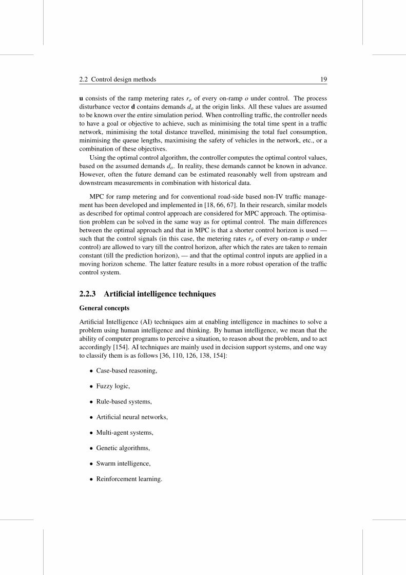
2.2.3 Artificial intelligence techniques
General concepts
Artificial Intelligence (AI) techniques aim at enabling intelligence in machines to solve aproblem using human intelligence and thinking. By human intelligence, we mean that theability of computer programs to perceive a situation, to reason about the problem, and to actaccordingly [154]. AI techniques are mainly used in decision support systems, and one wayto classify them is as follows [36, 110, 126, 138, 154]:
• Case-based reasoning,
• Fuzzy logic,
• Rule-based systems,
• Artificial neural networks,
• Multi-agent systems,
• Genetic algorithms,
• Swarm intelligence,
• Reinforcement learning.
20 2 State-of-the-Art
In this thesis, we will briefly discuss on case-based reasoning, fuzzy logic methods, rule-based systems, artificial neural networks, and multi-agent systems. For rest of the AI tech-niques, the interested readers are suggested to refer the above mentioned references.
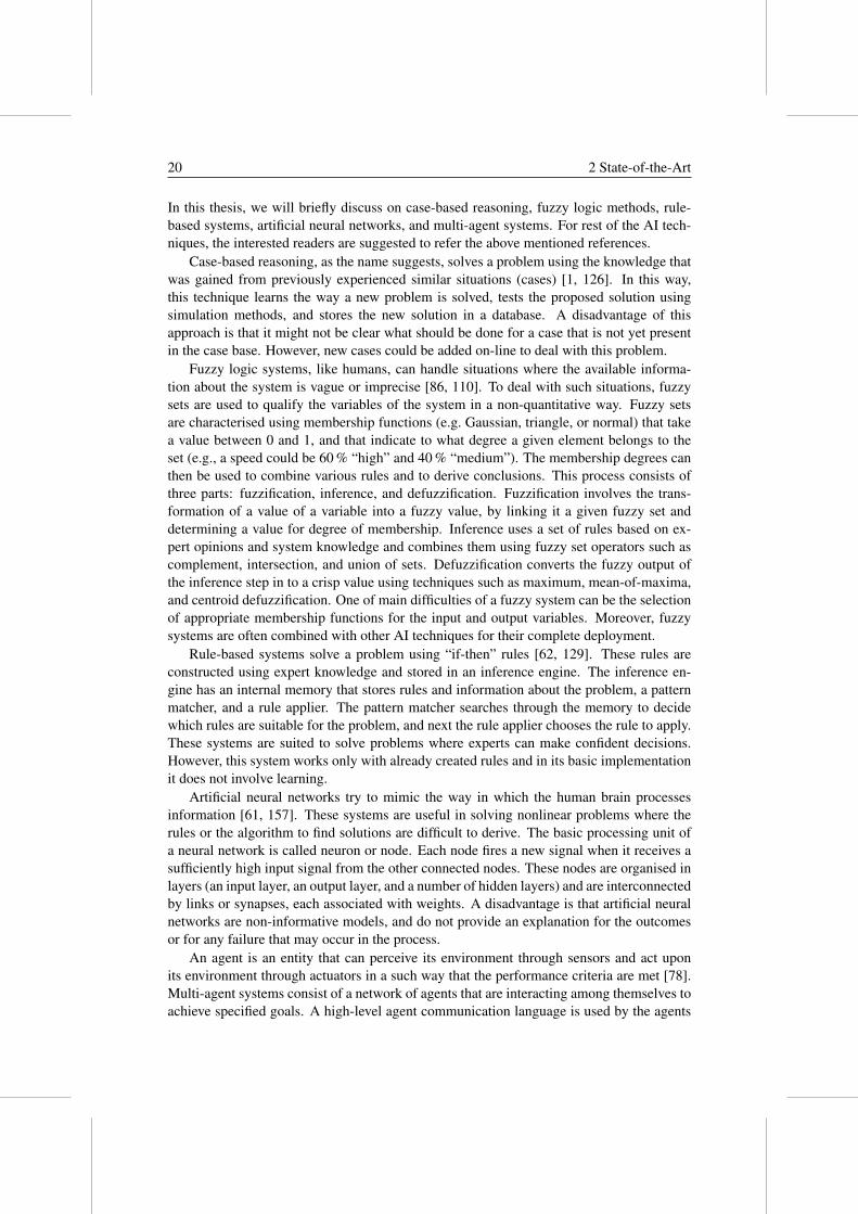
Case-based reasoning, as the name suggests, solves a problem using the knowledge thatwas gained from previously experienced similar situations (cases) [1, 126]. In this way,this technique learns the way a new problem is solved, tests the proposed solution usingsimulation methods, and stores the new solution in a database. A disadvantage of thisapproach is that it might not be clear what should be done for a case that is not yet presentin the case base. However, new cases could be added on-line to deal with this problem.
Fuzzy logic systems, like humans, can handle situations where the available informa-tion about the system is vague or imprecise [86, 110]. To deal with such situations, fuzzysets are used to qualify the variables of the system in a non-quantitative way. Fuzzy setsare characterised using membership functions (e.g. Gaussian, triangle, or normal) that takea value between 0 and 1, and that indicate to what degree a given element belongs to theset (e.g., a speed could be 60 % “high” and 40 % “medium”). The membership degrees canthen be used to combine various rules and to derive conclusions. This process consists ofthree parts: fuzzification, inference, and defuzzification. Fuzzification involves the trans-formation of a value of a variable into a fuzzy value, by linking it a given fuzzy set anddetermining a value for degree of membership. Inference uses a set of rules based on ex-pert opinions and system knowledge and combines them using fuzzy set operators such ascomplement, intersection, and union of sets. Defuzzification converts the fuzzy output ofthe inference step in to a crisp value using techniques such as maximum, mean-of-maxima,and centroid defuzzification. One of main difficulties of a fuzzy system can be the selectionof appropriate membership functions for the input and output variables. Moreover, fuzzysystems are often combined with other AI techniques for their complete deployment.
Rule-based systems solve a problem using “if-then” rules [62, 129]. These rules areconstructed using expert knowledge and stored in an inference engine. The inference en-gine has an internal memory that stores rules and information about the problem, a patternmatcher, and a rule applier. The pattern matcher searches through the memory to decidewhich rules are suitable for the problem, and next the rule applier chooses the rule to apply.These systems are suited to solve problems where experts can make confident decisions.However, this system works only with already created rules and in its basic implementationit does not involve learning.
Artificial neural networks try to mimic the way in which the human brain processesinformation [61, 157]. These systems are useful in solving nonlinear problems where therules or the algorithm to find solutions are difficult to derive. The basic processing unit ofa neural network is called neuron or node. Each node fires a new signal when it receives asufficiently high input signal from the other connected nodes. These nodes are organised inlayers (an input layer, an output layer, and a number of hidden layers) and are interconnectedby links or synapses, each associated with weights. A disadvantage is that artificial neuralnetworks are non-informative models, and do not provide an explanation for the outcomesor for any failure that may occur in the process.
An agent is an entity that can perceive its environment through sensors and act uponits environment through actuators in a such way that the performance criteria are met [78].Multi-agent systems consist of a network of agents that are interacting among themselves toachieve specified goals. A high-level agent communication language is used by the agents

2.2 Control design methods 21
for communication and negotiation purposes. Multi-agent systems can be applied to modelcomplex systems, but their dynamic nature and the interactions between agents may giverise to conflicting goals or resource allocation problems.
Control application for conventional traffic
Of the AI methods discussed above case-based reasoning and fuzzy logic are most oftendescribed in literature for traffic control purposes. In practice, rule-based systems are alsoused very often for traffic management and control.
Many decision support systems have been proposed for traffic management purposessuch as FRED (Freeway Real-Time Expert System Demonstration) [127, 159], the SantaMonica Smart Corridor Demonstration Project [82, 128], and TRYS [41, 94, 108].
In [41, 65, 73, 159] case-based systems are developed for a broad range of scenarios thatmay occur in a traffic network. This initial case-based system is in principle generated usinghistorical data or off-line simulations. In [65, 73] each scenario in the case base is evaluatedover a prediction horizon using simulation and can be characterised by “inputs” such as thecurrent traffic state, the traffic control measure applied (e.g., ramp metering, lane closures,etc.), or expected incidents (duration of incidents), and by “outputs” such as predicted av-erage values of the traffic states or predicted values for performance measures. Hence, thecase-based system maintains an input-output relation for each considered scenario. Oncethe initial case base is constructed, the traffic control centre can use this case-based systemas the basis for assessing a particular traffic problem and for determining the most appro-priate control scenarios. In case the current situation has not been addressed before, a new,real-life scenario of the traffic system can be evaluated and added to the case-based systemalong with effect of the control measures. Hence, learning and updating the case-basedsystem with newly encountered cases serves as the main advantage and motivation for theapplication of this system in the traffic control field.
Although this technique has been useful for controlling small networks, adding eachpossible case for a large-scale traffic network can be a difficult task. To solve this problemand to handle large-scale traffic networks, a possible solution has been proposed in [48].The solution of [48] considers a large-scale network as small subnetworks and uses fuzzylogic to combine different cases in the case base. By using fuzzy logic, a precise matchbetween the considered actual case and the relevant cases in the case-based system will notbe required.
As indicated before fuzzy systems can be used when accurate information of the trafficmodel is difficult to obtain or is not available [25, 94]. A fuzzy logic controller for rampmetering with a description of the various steps (fuzzification, inference, and defuzzifica-tion) is presented in [152]. Several fuzzy sets that can relate a variable (input, output) toa particular situation can be defined such as fuzzy sets for local speed, local traffic flow,queue occupancy, metering rate and local occupancy. Using fuzzification input variablessuch as speeds, flows, occupancy levels in the vicinity of the fuzzy ramp meter controller,and output variables such as metering rates can be translated to fit the defined fuzzy sets andto obtain values for the degree of membership. Next, these values are fed to the inferenceengine, which is constructed using a set of rules based on the experience of traffic controlcentre operators and on off-line simulations. These rules are to be kept as simple and easyto understand and to modify. The result of the inference is then transformed into a crisp

22 2 State-of-the-Art
Table 2.1: Comparison of control design methods
Control method Computational Constraints Future Model-based Scalabilitycomplexity (hard) inputs
Static feedback low no no not explicitly localisedOptimal control high yes yes model-based system-wideand MPCAI-based medium no no not explicitly localised
value in the defuzzification step, after which the final result is applied to the traffic systemor presented to the operator of the traffic control centre for further assessment.
Related work is described in [65, 106].
2.2.4 Comparison
We will now compare the control design methods discussed above based on the followingdirections:
• Computational complexity,
• Inclusion of hard constraints,
• Inclusion of future inputs,
• Model-based or not,
• Scalability.
The results of this analysis are shown in Table 2.1.
Computational complexity
Although the control design methods discussed above provide suboptimal performance (ex-cept for optimal control in the error-free case), the computational complexity of these meth-ods does vary depending on their application area. Static feedback control methods have lowon-line computational requirements, but they are in practice mainly applicable to small-scale systems. The on-line computational time required for AI techniques is somewhathigher but still much less than that of optimal control and MPC since the latter use on-line optimisation. All three control techniques also require off-line computations for modelidentification and model parameter calibration as well as for parameter tuning, training, orrule generation. These off-line computational requirements are mainly determined by themodel and its complexity (model order, degree of nonlinearity, etc.).
Inclusion of hard constraints
Consideration of hard constraints is an inevitable aspect to be included when controllingand managing traffic flows. Hard constraints are those that are to be necessarily satisfied.In general, static feedback control does not consider the external constraints. This lack ofinclusion of constraints also proves to be one of the major drawbacks of the static feedback
2.2 Control design methods 23
methods. Most AI methods also do not explicitly take (hard) constraints into account. Op-timal control and MPC on the other hand use optimisation and as a consequence they canexplicitly include hard constraints when determining the optimal control actions.
Inclusion of future inputs
Static feedback controllers do not consider the external future inputs. Since optimal controland MPC are prediction-based, they can also take into account knowledge about futureinputs (e.g., in traffic control one might detect traffic flows using detectors located upstreamand use this information). In general, AI techniques may also use predictions.
Model-based or not
All the control approaches explicitly or implicitly need a model to collect data and/or fortuning. However, by model-based we mean in particular whether the control method con-siders an explicit model in order to determine the optimal control actions. Although theparameters of a static feedback controller may be tuned using model-based simulations, thecontroller does not explicitly include a model of the traffic system inside it. In a similar waythe rules or cases of an AI-based controller may also be determined using simulation mod-els, but the models are not explicitly present in the controller. On the other hand, optimalcontrollers and MPC controllers in general use an explicit model of the (traffic) system as aprediction model when determining the optimal control actions.
Scalability
Based on the control structure used, we can categorise control and management systems[4, 52, 134] as follows:
• Centralised,
• Distributed,
• Decentralised,
• Hierarchical.
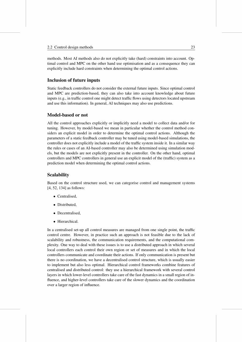
In a centralised set-up all control measures are managed from one single point, the trafficcontrol centre. However, in practice such an approach is not feasible due to the lack ofscalability and robustness, the communication requirements, and the computational com-plexity. One way to deal with these issues is to use a distributed approach in which severallocal controllers each control their own region or set of measures and in which the localcontrollers communicate and coordinate their actions. If only communication is present butthere is no coordination, we have a decentralised control structure, which is usually easierto implement but also less optimal. Hierarchical control frameworks combine features ofcentralised and distributed control: they use a hierarchical framework with several controllayers in which lower-level controllers take care of the fast dynamics in a small region of in-fluence, and higher-level controllers take care of the slower dynamics and the coordinationover a larger region of influence.

24 2 State-of-the-Art
In this context, static feedback controllers are mostly localised and are used to controlsmall-scale systems (in a central way) or as lower-level controllers in a hierarchical con-trol framework. Most AI-based control methods (except for multi-agent approaches) arealso mostly localised and can also be used in a hierarchical control framework. MPC (andoptimal control) determines the control actions based on the current and predicted futurestates of the system and thus allows for a system-wide coordination of the control actions.In principle, MPC can be used at all levels of a hierarchical control framework but due toits computational complexity it is less suited for the lower levels. In addition, recently somedistributed MPC methods have been developed [31].
In this section we have presented a brief overview of applied traffic control methods thatuse currently existing traffic control measures. In the next sections we will consider futuretraffic control systems based on intelligent vehicles and automated highway systems.
2.3 Intelligent vehicles and traffic control
2.3.1 Intelligent vehicles
We can divide IV application areas into three categories depending on the level of supportprovided to the driver [22]:
• Advisory systems use a human machine interface (HMI) (e.g., optic or acoustic) toprovide an advisory or warning to the drivers. Some examples include blind spotwarning, parking assistance, lane departure warning systems, and drowsy driver mon-itoring.
• Semi-autonomous systems can take partial control of vehicle manoeuvres and oftenuse haptic (meaning “based on the sense of touch”) measures to assist the driver andcan take partial control of vehicle manoeuvres. Examples are an intelligent speed ad-aptation system using an active accelerator pedal that exerts a counterforce at speedsover the speed limit, or a forward collision mitigation or avoidance system that firstwarns the driver via seat vibrations and next starts to brake in case the driver does notreact to the warning.
• Fully autonomous systems take complete control of vehicle operations and eliminatethe driver from the control loop. Examples include fully automated adaptive cruisecontrol and anti-lock braking systems.
IV-based control measures can be further classified based on their manoeuvres [23]:
• Lateral sensing and control systems assist drivers in controlling the lateral movementsof the vehicle. Applications of such systems are lane departure warning systems, lanechange assist systems, and parallel parking assist systems.
• Longitudinal sensing and control systems mainly help in controlling forward andbackward movements of the vehicle, and maintaining safe speeds and safe inter-vehicle distances. Typical applications are adaptive cruise control, forward collisionwarning systems, and intelligent speed adaptation.

2.3 Intelligent vehicles and traffic control 25
• Integrated lateral and longitudinal sensing and control systems provide both lateraland longitudinal support to the driver. Such applications can combine the functional-ities of adaptive cruise control and lane keeping assistance systems to assist the driverin performing manoeuvres.
2.3.2 IV-based traffic management
The currently implemented traffic control and management systems are mainly using intel-ligence in the roadside infrastructure for controlling and managing the traffic system, How-ever, such a system does not make use of the significant benefits offered by the intelligence— including the additional control, sensing, and communication capabilities — provided byIVs. So one way to improve performance and safety of the current transportation systemsis by applying automation and advanced intelligent control methods to roadside infrastruc-ture and vehicles. Based on the way a traffic control and management approach utilises theautomated vehicles, we can categorise the ongoing research on automated driving for trafficmanagement as follows:
• Automated platooning,
• Autonomous IVs.
We will now briefly explain these two approaches.
An interesting functionality that is allowed by full automation is to arrange the vehiclesin closely spaced groups called “platoons” [28]. In a platoon, the first vehicle is called“leader” and the remaining vehicles are called “followers”. To avoid collisions, intra-platoon spacing (i.e., vehicle spacing within a platoon) is kept very small and the inter-platoon spacing is kept larger [97, 149]. In the literature, many control frameworks, mainlyintended to study inter-vehicle communication technologies and to control the platoon man-oeuvres in cooperation with the roadside infrastructure, have been developed and investig-ated [7, 63, 76, 124, 145]. Also, frameworks that allow communication between the (par-tially or fully) automated individual vehicles and with the nearby roadside infrastructurehave been proposed [42].
The other main category of IV-based traffic management approaches involves individualautonomous IVs and is mainly based on self-organisation and distributed intelligence amongthe automated vehicles with no control from the roadside infrastructure. In this autonomousdriving system, the vehicles try to aggregate themselves in groups, make their decisionsbased on local information only, and perform manoeuvres in a cooperative fashion. Mod-elling and analysis of such group behaviour mechanisms in traffic management is an activearea of research [54, 96, 100, 119].
In this chapter, we focus on the first approach, as this approach most probably allowsfor a smoother transition from the current, exclusively roadside-based traffic control systemtowards a mixed IV-roadside traffic management system in which the intelligence betweenthe roadside infrastructure and the intelligent vehicles are integrated so as to improve thetraffic performance.

26 2 State-of-the-Art
2.3.3 IV-based control measures
In this section, we discuss various IV technologies that support both roadside traffic controlmeasures and automated platoons of IVs. The main functional areas of IV systems thatsupport traffic management and control on freeways are:
• Adaptive Cruise Control (ACC),
• Intelligent Speed Adaptation (ISA),
• Dynamic route guidance.
Adaptive cruise control
Many vehicles have already been deployed with partial automation of the driving task bythe use of the standard conventional cruise control [125].
An Adaptive Cruise Control (ACC) system is a radar-based system that extends theconventional cruise control system and that is designed to sense the vehicle immediately infront on the same lane, and to automatically adjust the speed of the equipped vehicle to thatof the preceding vehicle so as to maintain a safe inter-vehicle distance [45, 47]. If there isno predecessor, then ACC retains the preset speed that was selected by driver.
Variations of ACC are available in the market, among which high-speed ACC and stop-and-go ACC are popular [120]. High-speed ACC uses a radar to measure speed and distanceof the vehicle ahead so as to maintain a safe distance between the vehicles. This ACC systemis designed to operate at medium (above 40 km/h) to higher speeds, because at this rangeof speeds, a sensor can discriminate between non-moving targets and moving vehicles. Aradar can sense a low relative velocity with respect to a moving predecessor and a highrelative velocity with respect to stationary objects. However, high-speed ACC systems havedifficulties to operate at low speeds. Stop-and-go ACC is designed to work with low speeds(0 km/h to 40 km/h) that prevail on urban roads and in congested traffic. Basically, thestop-and-go ACC acts as a distance controller rather than a speed controller.
Although ACC vehicles are able to handle many traffic situations reliably [113], thereexist some adverse traffic conditions such as short-headway cut-ins, or sudden and strongdeceleration of the up-front vehicle that prevent the ACC from sensing and reacting to thesituation immediately. Cooperative ACC is a further enhancement of ACC systems thatutilises existing communication technologies (e.g., ad hoc wireless networks) to obtain real-time information about the speed, acceleration, braking, position, headway, and yaw rate ofthe preceding vehicle in order to maintain a safe but small headway, and to ensure smoothdriving [147].
Using cooperative ACC, vehicles can travel at reduced headways. Hence, with reducedheadways between vehicles, traffic flow can be improved.
Intelligent speed adaptation
A standard speed limiter is a system that restricts the speed of the vehicle when the drivertries to exceed the maximum allowed driving speed. When the speed limiter is incorporatedwith the intelligence to adjust the maximum driving speed to the speed limit specified by theroadside infrastructure or to the prevailing location-based legal speed limit, and to provide

2.4 Control frameworks and architectures for IVHS 27
feedback to the driver when that speed limit is exceeded, then we get the technology calledIntelligent Speed Adaptation (ISA) [24, 39].
ISA systems can be characterised based on the extent to which the driver is made awareof the situation when the speed limit is exceeded. This results in advisory, voluntary, andmandatory systems [32, 141].
Another characterisation for ISA systems can be made based on the speed limit itself asa fixed or a dynamic speed limit. In the fixed case, the driver is informed about the speedlimit, which could be obtained from a static database. A dynamic speed limit system takescurrent road conditions such as bad weather, slippery roads, or major incidents into accountbefore prescribing the speed limit.
ISA can influence the traffic flow by limiting the maximum speed of the vehicles de-pending upon the actual traffic flow conditions. As such congestion can be delayed oralleviated by delaying vehicles so that by the time they arrive at a congested region thecongestion has diminished or has already been dissolved.
Dynamic route guidance
Nowadays, many individual vehicles are equipped with a route guidance or navigation sys-tem. Based on current or expected travel times, and delays due to congestion, a route guid-ance system advises a driver about the “best” route he can take to reach his requested destin-ation [103, 131, 153]. This route recommendation mainly depends on the vehicle’s currentlocation. Using a GPS, the position of the vehicle can be determined accurately. This in-formation can be looked up on a digital road map and be used to determine the possibleroutes to reach the destination. These route recommendations may be calculated within theequipped vehicle or communicated to the vehicle from the local traffic centre.
A possible categorisation of route guidance systems is static versus dynamic route guid-ance. When the possible routes are computed based on the average traffic conditions (e.g,based on historical data or on the type of roads (such as urban corridor, highway, local road,etc.)), then this scheme is referred to as static route guidance system. If the current trafficconditions such as traffic jams, dynamic speed limits, and on-line predictions of travel timesusing real-time traffic data are taken into account while computing the route recommenda-tions, then we have a dynamic route guidance system [84, 155].
Dynamic route guidance systems can improve the traffic flow, by providing route re-commendations to the vehicles such that congestion is prevented from occurring or suchthat the effects of traffic jams are mitigated.
2.4 Control frameworks and architectures for IVHS
Now we discuss the most important control architectures that have been developed for link-ing the roadside infrastructure and automated platoons. In particular, we consider the PATH,Dolphin, Auto21 CDS, CVIS, SafeSpot, and PReVENT frameworks.
2.4.1 PATH framework
The PATH architecture [28, 74, 133, 149, 150] mainly focuses on the coordination of bothroadside-vehicle and inter-vehicle activities.
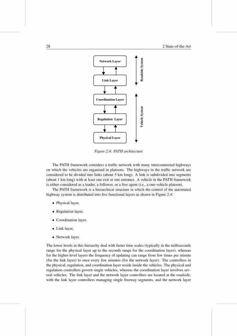
28 2 State-of-the-Art
Coordination Layer
Link Layer
Regulation Layer
Physical Layer
Ro
ad
sid
e S
yst
emV
ehic
le S
yst
em
Network Layer
Figure 2.4: PATH architecture
The PATH framework considers a traffic network with many interconnected highwayson which the vehicles are organised in platoons. The highways in the traffic network areconsidered to be divided into links (about 5 km long). A link is subdivided into segments(about 1 km long) with at least one exit or one entrance. A vehicle in the PATH frameworkis either considered as a leader, a follower, or a free agent (i.e., a one-vehicle platoon).
The PATH framework is a hierarchical structure in which the control of the automatedhighway system is distributed into five functional layers as shown in Figure 2.4:
• Physical layer,
• Regulation layer,
• Coordination layer,
• Link layer,
• Network layer.
The lower levels in this hierarchy deal with faster time scales (typically in the millisecondsrange for the physical layer up to the seconds range for the coordination layer), whereasfor the higher-level layers the frequency of updating can range from few times per minute(for the link layer) to once every few minutes (for the network layer). The controllers inthe physical, regulation, and coordination layer reside inside the vehicles. The physical andregulation controllers govern single vehicles, whereas the coordination layer involves sev-eral vehicles. The link layer and the network layer controllers are located at the roadside,with the link layer controllers managing single freeway segments, and the network layer

2.4 Control frameworks and architectures for IVHS 29
controllers handling entire networks.The same temporal and spatial division across different layers is also present in other frame-works that will be discussed in the next sections, such as the Dolphin framework and theAuto21 CDS framework.
Now we discuss each layer of the PATH framework in more detail, starting from the bottomof the hierarchy.
The physical layer of each vehicle involves the actual dynamics of the vehicle. This layerhas controllers that perform the actuation of the steering wheel, throttle, and brakes. It alsocontains the sensors in the vehicle that collect information about the speed, the acceleration,and the engine state of the vehicle, and send it to the regulation layer.
The regulation layer controller executes the tasks specified by the coordination layer(such lane changes, and splits or merges of platoons) by converting them into throttle, steer-ing, and braking inputs for the actuators of the vehicle. The regulation layer controllerwithin each vehicle uses feedback control laws to execute the lateral and longitudinal man-oeuvres and also notifies the coordination controller in case of any failures or unsafe out-comes of the manoeuvres.
Next in the hierarchy is the coordination layer with a controller residing inside eachvehicle. This layer receives the commands from the link layer (such as set-points or profilesfor the speeds, or platoon sizes). A coordination layer controller allows coordination withother neighbouring platoons using messages or communication protocols, and checks whichmanoeuvres (like lane changes, splits, or merges) have to be performed by a vehicle in orderto achieve the platoon size or path trajectory specified by the link controller.
The next layer in the control hierarchy is the link layer. This layer has a controllerlocated at each link and is mainly responsible for path and congestion control. Each linkcontroller receives commands from the network layer (such as routes for the platoons) andbased on these commands, the link controller calculates the maximum platoon size, and theoptimum platoon velocity for each segment in the link it is managing. The link controlleralso sets the local path (which lane to follow) for each platoon.
The top layer in the hierarchy is called the network layer. At this layer, the controllercomputes control actions that optimise the entire network. Its task is to assign a route foreach vehicle or platoon that enters the highway ensuring that the capacity of each potentialroute is utilised properly. There will be one network layer controller for the consideredtraffic network.
The PATH framework has also been used in other projects such as, e.g., the AHSRA(Advanced Cruise-Assist Highway System Research Association) project launched by theJapanese Ministry of Land, Infrastructure and Transport [2].
2.4.2 Dolphin framework
The Japanese Dolphin framework developed in [144, 145] is similar to the PATH architec-ture. The name of this framework is inspired by the way in which groups of dolphins moveand which is mimicked by the automated vehicles in the platoons. The Dolphin frameworkconsiders vehicles to be arranged as platoons and develops inter-vehicle communicationtechnologies to carry out cooperative driving for the purpose of smooth merging and lanechanging.

30 2 State-of-the-Art
Inter−vehicle
communication
Traffic Control Layer
Vehicle Management
Layer
Vehicle Control Layer
Veh
icle
Sy
stem
Criteria Road−vehiclecommunication
Ro
ad
sid
eS
yst
em
Commands Sensor data
Figure 2.5: Dolphin architecture for cooperative driving
The Dolphin framework is composed of three layers as shown in Figure 2.5:
• Vehicle control layer,
• Vehicle management layer,
• Traffic control layer.
The vehicle controller within each vehicle senses the states and the conditions ahead ofthe vehicle such as vehicle speed and acceleration and sends this information to the vehiclemanagement layer. The vehicle controller also receives commands for the vehicle’s steeringactions and determines the actions for the vehicle actuators.
The vehicle management controller, which resides in each vehicle, receives suggestionsfor the movements of the vehicle from the traffic controller via road-vehicle communicationand also considers the messages from the neighbouring vehicles via inter-vehicle commu-nication and the data received from the basic vehicle control layer. This controller de-termines the movements of the individual vehicle under platoon-based driving. Lateral andlongitudinal control actions for the platoon leader or free agent are determined by this layerusing, e.g., a localisation function by GPS and a digital map of the traffic network. Thevehicle management controllers in the follower vehicles determine both the lateral and thelongitudinal control commands for the vehicle they control.
The traffic control layer is the top layer and it includes roadside IVHS equipment likesign boards, conventional lane markers, and variable message signs, as well as logic suchas laws, rules, and common sense. There is only one traffic control layer common to allthe vehicles and it is part of the roadside infrastructure. The traffic layer consists of severaldistributed controllers, each of which determines advisory instructions for the vehicles inits own neighbourhood and sends these instructions to the vehicle management layer. Forexample, the instructions could be to maintain a small inter-vehicle distance between thefollowers in a platoon, and to support an autonomous driving for the leaders in a platoon.
2.4.3 Auto21 CDS framework
The Auto21 Collaborative Driving System (CDS) framework [7] is mainly inspired by theconcepts of the PATH and Dolphin architectures. The CDS architecture considers platoons

2.4 Control frameworks and architectures for IVHS 31
communication
Intra−platoon
communication
Management Layer
Networking
communication
LinkingInter−platoon
communication
Intra−platoon
communication
Syst
emV
ehic
le S
yst
em
Plans
Traffic Control Layer
Coordination
Road
sid
e
CriteriaRoad−vehicle
Inter−platoon
Actions
Planning
Sensor data Commands
Guidance Layer
Figure 2.6: Auto21 CDS architecture for cooperative driving
of cars as autonomous agents and uses cooperative ACC technologies to support platoon-based driving. The CDS framework employs an inter-vehicle coordination system that canensure coordination of vehicle activities during their merge and split operations from a pla-toon and that can maintain stability among the vehicles in a platoon. The hierarchical ar-chitecture of the Auto21 CDS framework consists of the following three layers as shown inFigure 2.6:
• Guidance layer,
• Management layer,
• Traffic control layer.
In every vehicle there is a guidance layer controller that senses the state of the vehicleand sends information on the position, speed, acceleration, etc. of the vehicle to the man-agement layer. This controller also receives commands from the management layer, whichare then translated into control actions for the throttle, braking, and steering.
The management layer is the main contribution of the CDS framework. The manage-ment layer contains several controllers, one for each vehicle. A management layer con-troller is responsible for determining the movements of the vehicle it manages using theinformation received from the traffic control layer, and makes sure that vehicle coordinationconstraints are satisfied through inter-vehicle communication. This layer is subdivided intocoordination and planning sublayers that work cooperatively. The coordination sublayer hasa linking module that communicates with the traffic control layer to receive suggestions forthe lane change actions and that manages the inter-platoon activities. Once the linking mod-ule has made a choice on which the action to perform, the manoeuvres are executed (such asmerge or split from a platoon) by a networking module, which coordinates the intra-platoonactivities. The planning sublayer is responsible for making the plans to execute the man-oeuvres inside the platoons. These plans are constructed in cooperation and coordinationwith the networking module.

32 2 State-of-the-Art
Roadside infrastructure
Vehicle
Handheld
Central
CVIS Subsystems
Existing
vehicle systemtraffic management
roadside system &
Existing
system
Figure 2.7: CVIS set-up
The traffic control layer is located in the roadside infrastructure and provides sugges-tions on desired speeds for segments, maximum platoon sizes, etc. The traffic control layeralso supports the linking module (of the management layer) for making decisions on inter-platoon coordination actions [60].
2.4.4 CVIS
CVIS (Cooperative Vehicle-Infrastructure Systems) [42, 146] is a European research anddevelopment project that aims to design, develop, and test technologies that allow commu-nication between the cars and with the roadside infrastructure, which in turn will improveroad safety and efficiency, and reduce environmental impact. Traffic systems with CVIStechnologies select a suitable communication medium depending on user requirements andavailable media, and allow cars to communicate in a secure way using wireless technologies.
CVIS operates with existing traffic control and management centres, roadside infrastruc-tures, and vehicle systems. The complete system can be considered as a single-level archi-tecture with the existing systems and CVIS operating at the same level. Various networksand communication protocols have been developed within CVIS to enable communicationbetween different subsystems. The time scale for this architecture ranges from minutes tohours.
A CVIS system is composed of four subsystems as shown in Figure 2.7: central, hand-held, vehicle, and roadside subsystems. The central subsystem is a basically a service pro-vider for the vehicle or the roadside infrastructure. Typical examples of central subsystemsinclude traffic control and service centres, and authority databases. The handheld subsys-tem provides services such as pedestrian safety and remote management of other CVISsubsystems by allowing access to the CVIS system using PDAs and mobile phones. Thevehicle subsystem is comprised of on-board systems and includes vehicle sensors and ac-tuators, and equipment for vehicle-vehicle and vehicle-infrastructure communication. Theroadside subsystem corresponds to the intelligent infrastructure that operates at the roadsideand includes traffic signals, cameras, variable message signs, etc.
2.4.5 SafeSpot
SafeSpot [130, 143] is a research project funded by the European 6th Framework Programon Information Society Technologies. The main objective of this project is to improve roadsafety using advanced driving assistance systems and intelligent roads. The safety marginassistant developed by the SafeSpot project uses advanced communication technologies to

2.4 Control frameworks and architectures for IVHS 33
Local dynamic mapHaptic
Visual
Acoustic
Sensors
Infrastructure dataVehicle data
Human MachineInterface Safety margin assistant
Platform Domain
Application Domain
Figure 2.8: SafeSpot set-up
Action
Decision
Perception
Figure 2.9: PReVENT set-up
obtain information about the surrounding vehicles and about the roadside infrastructure.This safety margin assistant can detect dangerous situations in advance and can make thedriver aware of the surrounding environment using a human machine interface as shown inFigure 2.8. The time scale for this architecture ranges from seconds to minutes.
2.4.6 PReVENT
PReVENT [121] is a European automotive industry activity co-funded by the EuropeanCommission. The main focus of the PReVENT project is to develop preventive applicationsand technologies that can improve the road safety. These safety applications use in-vehiclesystems to maintain safe speeds and distances depending on the nature and severity of theobstacles, and to provide instructions and to assist the drivers in their driving tasks so as toavoid collisions and accidents.
The PReVENT architecture introduces a three-layer approach as shown in Figure 2.9with the following layers:
• Perception layer,

34 2 State-of-the-Art
• Decision layer,
• Action layer.
All these layers are located within the vehicle. From the perception layer upward to theaction layer, the time complexity and update frequency of states typically ranges from mil-liseconds to seconds.
The perception layer uses on-board sensors (such as radar, cameras, and GPS receivers)in conjunction with digital maps and allows vehicle-to-vehicle and vehicle-to-infrastructurecommunication.
The decision layer assesses dangerous situations ahead of the vehicle and determinesrelevant actions that are needed to avoid such situations. The controller then passes thisdecision to the action layer.
The action layer then issues warnings to the driver about the severity of the situationthrough an appropriate human machine interface or through vehicle actuators such as thesteering wheel or the brakes.
2.5 Comparison of the IVHS frameworks
In Section 2.4 we have discussed various existing frameworks and architectures for IVHS-based traffic management. Now, we will compare the frameworks based on the followingfeatures:
• Control objectives,
• Type of formation control (platoons or single cars),
• Intelligence at roadside and/or in vehicles,
• Presence and type of communication and/or coordination,
• Time scales involved.
The results of this analysis are shown in Table 2.2.
Control objectives
For the PATH framework, the focus is primarily on designing and developing lateral andlongitudinal controllers that allow automation of vehicles in a platoon and platoon man-oeuvres. The PATH program has also developed coordination and communication tech-niques that are required during such manoeuvres. In addition, the roadside controllers inthe PATH framework (i.e., the network and link layer controllers) determine the activitiesthat need to be carried out in different freeway segments to avoid congestion. The Dol-phin framework is vehicle-oriented, which means that the framework is mainly intended tostudy the inter-vehicle communication technologies that can be used to control a group ofplatoons that reside on neighbouring lanes and to support their manoeuvres. The AUTO21CDS framework mainly aims at developing communication and coordination methodolo-gies for merging and splitting actions within the platoon (intra-platoon manoeuvres). This

2.5 Comparison of the IVHS frameworks 35
Table 2.2: Comparison of the various IVHS frameworks (in this table “veh” stands for
“vehicles”, “V2V” means “vehicle-vehicle”, and “V2I” is short for “vehicle-
infrastructure”)
Framework Control Formation Intelligence Communication Time
objectives control & coordination scale
PATH platoon manoeuvres platoons road/veh V2V/V2I ms–h
traffic flow efficiency
Dolphin platoon manoeuvres platoons (road)/veh V2V ms–h
Auto21 CDS intra-platoon platoons (road)/veh V2V ms–hmanoeuvres
CVIS traffic efficiency cars road/veh V2V/V2I min-h
SafeSpot prevent/avoid road cars (road)/veh V2V/V2I s–minaccidents
PReVENT car safety cars veh V2V ms–s
framework uses an inter-platoon coordination model that was developed by the PATH pro-ject [8]. The objective of the CVIS project is to develop controllers and communicationtechnologies for implementing a cooperative vehicle-highway system.
The PATH, Dolphin, AUTO21 CDS, and CVIS frameworks have developed controlmethodologies to be implemented in the roadside infrastructure to improve the traffic flowor in vehicles to allow automation of driving tasks. On the other hand, SafeSpot and PRe-VENT focus on improving the road safety by avoiding or preventing accidents, and they aimat integrated safety, with an emphasis on the potential of communication between vehiclesand between vehicles and roadside systems.
Type of formation control
The frameworks usually consider the vehicles to be controlled either as part of higher-levelentities such as platoons, or as individual vehicles. The PATH, Dolphin, and Auto21 CDSframeworks allow platooning. On the other hand, SafeSpot, PReVENT, and CVIS do notuse platoons.
Intelligence at roadside and/or in vehicles
The PATH framework allows involvement of both roadside infrastructure and vehicles forimproving traffic performance. Although the Dolphin and the Auto21 CDS frameworksconsider distributed intelligence between roadside infrastructure and vehicles, the roadsideinfrastructure only provides suggestions and instructions to the vehicles. The platoons arenot obliged to follow these suggestions. CVIS and SafeSpot incorporate intelligence inboth vehicle and roadside infrastructure. PReVENT also includes distributed intelligencebut with the main focus on vehicle intelligence.

36 2 State-of-the-Art
Presence and type of communication and/or coordination
Almost all the frameworks and projects have designed and developed technologies for inter-vehicle and roadside-vehicle communication for coordination of activities. Specifically,PATH has developed dedicated communication protocols [57, 76] and the Dolphin frame-work has developed a wireless local access network model for vehicle following, and inter-vehicle communication technologies for platoon manoeuvre coordinations [144]. For thecoordination of tasks within the platoons, the AUTO21 CDS framework allows both a cent-ralised set-up (i.e., the platoon leader instructs intra-platoon manoeuvres) or a decentralisedset-up (i.e., all the members of the platoon are involved in the coordination)
SafeSpot, PReVENT, and CVIS focus on the issue of developing communication tech-niques that can be implemented in existing traffic networks and that can also be extended toAHS.
Time scales involved
The time scales involved for the PATH, Dolphin, and Auto21 CDS frameworks vary frommilliseconds to hours as one traverses from dynamics of the vehicle up to the roadside infra-structure levels. The time complexity and update frequency typically ranges from minutesto hours for CVIS, from seconds to minutes for SafeSpot, and from milliseconds to secondsfor PReVENT.
2.6 Outlook
In this section we first sketch how the control design methods presented in Section 2.2 couldeventually be applied within the various IVHS control architectures of Section 2.4. We alsoindicate the challenges and issues that still have to be addressed to get a full-fledged andcomplete IVHS-based traffic management and control system.
2.6.1 Application to IVHS
In relation to IVHS, longitudinal controllers for IVs inside platoons such as cooperativeACC controllers can be implemented using static feedback control. In particular, we nowdiscuss how the accelerations for the follower vehicles within a platoon could be calculatedusing a static feedback controller. The follower vehicles in a platoon should use their on-board ACC system to maintain short intra-platoon distances. Hence, an ACC algorithmcould consist of a combined speed and distance controller as described in [77]:
ai(k) = K2(href,i(k)− (xi+1(k)− xi(k)))+ K3(vi+1(k)− vi(k))
where ai(k) is the acceleration for vehicle i at time t = kT , vi(k) is the speed of vehicle i attime t = kT , xi(k) is the longitudinal position of the rear of vehicle i at time t = kT , href,i isthe reference distance headway for vehicle i, and K2 and K3 are controller parameters. Thereference distance headway is defined as follows:
href,i(k) = S0 + vi(k)Thead,i + Li , (2.1)

2.6 Outlook 37
[s]
tim
e
hi
Li∆ i
s i
XX i
Xi X
+1
i+1
space [m]
ii
h is distance headway
time headway
Figure 2.10: Time-space plot illustrating the definition of the time headway hi and the dis-
tance headway si for vehicle i
where S0 is the minimum safe distance headway that is to be maintained at zero speed, Thead,i
is the desired time headway for vehicle i, and Li is the length of vehicle i. These definitionsare illustrated using two vehicles i and i + 1 travelling on a single lane in a time-spacecoordination system as shown in Figure 2.10. The time and distance directions are shownin vertical and horizontal axes respectively. The time headway is more often consideredrather than distance headway because of its simplicity and ease of measuring. In practice,the distance headway can be obtained from photos.
Optimal control and in particular MPC can be applied either in vehicle controllers orin roadside controllers. For a low-level control tasks involving manoeuvres of individualvehicles such as ACC or ISA, which need frequent updates of the control signal (e.g., theacceleration), these methodologies may prove to be very slow due to the computationalcomplexity involved. However, MPC is excellently suited for higher-level IV-based trafficcontrol and management purposes and to determine optimal speeds, lane allocations, andon-ramp release times for the platoons. MPC offers a strategy that can determine the controlactions based on the current and predicted future states of the traffic network, and that canoptimise the performance objective assigned to roadside infrastructure over a given time ho-rizon subject to the operational constraints and the constrained imposed on them. Moreover,the feedback and the receding horizon approach of MPC allow to reduce the effects of pos-sible mismatch errors between the actual real-world traffic flows and the predicted trafficflows. Some results in this direction are described in [13, 14]. In addition, since MPC isan optimisation-based approach, it is able to deal with the many different, often conflict-ing objectives (e.g., safety versus efficiency) that play a role in IVHS through the use ofmulti-criteria optimisation [107].
Fuzzy controllers can be used to implement an ACC controller using the deviations inspeeds and distances as input variables. A typical example of such an application is dealtwith in [71]. Moreover, fuzzy control can also be used to assist in making decisions fortraffic management purposes. On the other hand, case-based reasoning will be more suitablefor traffic planning and management purposes than for individual vehicle controllers.
2.6.2 Challenges and open issues
Now we discuss the main technological, economical, and societal challenges that will haveto be addressed when actually implementing an IVHS systems.

38 2 State-of-the-Art
Although we have indicated above how control design methods such as static feedbackcontrol, MPC, and AI-based control could be used for IVHS and traffic management andcontrol systems based on intelligent vehicles and platoons, real integration of these methodsis still lacking. This is one of the challenges that still have to be addressed. However, thedeployment of these control design methodologies does not ensure stability and robustnessof the traffic system since IVHS and IVs are non-linear and often even hybrid (i.e., theyexhibit both continuous dynamics and discrete-event behaviour (switching)).
The new control methods developed within PATH and the other frameworks have mainlyfocused on the lower layers, i.e., the coordination between the vehicles and the platoons, andhave not really focused on higher-level traffic management aspects beyond the single free-way level such as route guidance and network-wide coordination. Moreover, the segmentconcepts used in PATH may lead to difficulties when dealing with very long platoons. In-deed, when the platoon size is very large, then a platoon might cover several segments,and then it might be difficult for the roadside controllers involved to assign the appropriateactivities for the platoon, and also for the involved vehicle controllers to coordinate theiractivities. This raises two important open problems: platoon formation and scalability.
In literature there are no strict rules available on how to form platoons and on how manyvehicles to include in a platoon. This can either be specific to a given road or to a destination.There are few articles that deal with vehicle sorting with respect to platoon sizes and platoonformation time, and also on the design of platoon manoeuvre protocols [59, 75].
Some of IVHS frameworks such as the PATH, Auto21 CDS, and Dolphin frameworksare by nature hierarchical and offer thus a certain degree of scalability with regard to net-work size. Other frameworks such PReVENT, SafeSpot, and CVIS are not explicitly hier-archical and are thus not inherently scalable with regard to network size. However, noneof the frameworks explicitly addresses scalability and the scalability of the frameworks hasnot yet been investigated in detail in literature. So this is also a topic for future research. Inaddition, scalability with regard to platoon sizes is also an open issue.
Hence, one of the major requirements is the development of a (new) integrated hier-archical traffic management framework for IVHS and the design and implementation of ap-propriate control methods for such a framework. Moreover, the full automation present inIVHS may also lead to new traffic control measures that can currently not be implemented,such as “real-valued” speed limits for more accurate control, smoother merging at on-rampsthrough speed and spacing control, etc. These new measures should also be accommodatedin the control framework.
The technical issues outlined above are still open and need to be addressed. Moreover,the IVHS approach requires major investments to be made by both the government (or thebody that manages the highway system) and the constructors and owners of the vehicles.Since few decisions are left to the driver and since the AHS assumes almost complete controlover the vehicles, which drive at high speeds and at short distances from each other, a strongpsychological resistance to this traffic congestion policy is to be expected. In addition,the fact that vehicles can be tracked through the entire network may raise some concernsregarding privacy and liability issues.
Another important question is how the transition of the current highway system to anAHS-based system should occur and — once it has been installed — what has to be donewith vehicles that are not yet equipped for IVHS. As an intermediate step towards IVHSthe current highway management system could start to communicate with the IVs and use

2.7 Summary 39
information obtained from, e.g., the route guidance system of the IVs in order to moreaccurately forecast traffic loads. Other transition issues that have to be taken into accountare [50]: How will the system be funded? What types of accidents can be expected to occurin AHS, in what numbers, and with what consequences? Will bi-directional communicationand transfer of information be allowed between IVs and roadside infrastructure? What arethe legal implications of an accident, especially if it were caused by system error or a systemoversight? How will an AHS implementation be coordinated on an international level? etc.
2.7 Summary
We have presented on overview of traffic management and control frameworks for IVHS.First, we have given a short survey of the main control design methods currently used forfreeway traffic control. Next, we have discussed various traffic management architecturesfor IVHS such as PATH, Dolphin, Auto21 CDS, CVIS, SafeSpot, and PReVENT. Theframeworks have been compared in a qualitative way and we have sketched how the currenttraffic control methodologies could fit in an IVHS-based traffic control set-up. Finally, wehave identified some open issues and future challenges in the further implementation andactual deployment of IVHS traffic management systems.

40 2 State-of-the-Art

Chapter 3
A New Traffic Management
Framework for IVHS
3.1 Introduction
Based on an extensive survey of existing IV-based traffic management approaches andframeworks, the main components and results of which are discussed in Chapter 2, wenow propose a new IV-based framework that combines several of the strong points of ex-isting architectures and that further enhances and extends them in several directions. Theobjective of the framework is to integrate the intelligence of roadside infrastructure and IVsystems with automation. We propose a framework that distributes the intelligence betweenroadside infrastructure and vehicles, that assigns the traffic control actions based on platoonsrather than on a segment concept, and that uses the IV-based control measures to improvethe traffic performance in terms of safety, throughput, and environment. We want also toinclude the advantages of other frameworks such as CarTalk, SafeSpot, Prevent, CVIS thatdesign and develop technologies for inter-vehicle and roadside/vehicle communication. Inthis chapter, we present the new hierarchical IV-based traffic control framework in moredetail.
3.2 IV-based control framework
The goal of the proposed framework is to use the additional measures and control handlesoffered by in-vehicle telematics that support platooning and to implement them in a hier-archical roadside/vehicle traffic management structure to substantially improve traffic per-formance in terms of safety, throughput, reliability, environment, and robustness. Theframework mainly aims at a multi-level control structure with local controllers at the lowestlevel and one or more higher supervisory control levels. Moreover, it will use a combina-tion and integration of techniques from computer science and control engineering in orderto obtain coordination at and across all control levels.
Our framework is inspired by the AHS platoon concept and uses IV-based control meas-ures to implement a next-level of traffic control and management, which shifts away from
41

42 3 A New Traffic Management Framework for IVHS
the rather global road-side traffic management to a more vehicle-oriented traffic manage-ment. We will consider both roadside-vehicle traffic management and interaction, and inter-vehicle traffic management and coordination. Although the PATH framework [74, 149, 150]includes both roadside infrastructure and vehicles, much of the research work was carriedon the vehicle control side. The roadside controllers determine the activities that need tobe carried out in different segments. However, when the platoon size is allowed to be longenough, then it might be difficult for the roadside controller to assign the activities as theplatoon resides in between two segments, and also for the vehicle controller to completethe activity within the specified space. For this reason, we use platoon-based roadside con-trollers (so without segments). In our framework, vehicles will travel as platoons. Everyplatoon will then have a leader vehicle and the rest of the vehicles, if any, as followers.The platoon leader uses ISA and the followers will be equipped with ACCs. In addition,in order to be able to deal with large-scale traffic network we will consider a hierarchicalcontrol structure with several layers each of which consist of several controllers (see Figure3.1). The reasons for selecting such a distributed, hierarchical control structure for trafficmanagement are:
• Scalability: Adding, altering, or removing layers can be easily executed without al-tering other layers in the architecture, i.e., a hierarchical structure is more flexible formodifications in problem size.
• Robustness: In case of any unexpected failures in one of the components, the frame-work in general, will still be able to complete its execution of planned tasks (gracefuldegradation).
3.2.1 Proposed control framework
A general structure of the proposed control architecture is shown in Figure 3.1. The archi-tecture consists of several layers, which can be characterised as follows:
Higher-level controllers
Higher-level controllers (area, regional, and supraregional) provide network-wide coordin-ation of the lower-level and middle-level controllers. For example, there could be an areacontroller to control/supervise the activities of a collection of roadside controllers. In turn,a group of area controllers could be supervised by regional controllers, etc.
Roadside controller
The roadside controller in the hierarchy uses IV-based control measures to improve thetraffic flow. The controller assigns desired speeds for each platoon (ISA), safe distancesbetween platoons (Cooperative ACC), metering values on the on-ramps and off-ramps (rampmetering), desired platoon sizes, provides dynamic route guidance for the platoons, and alsoinstructs for merges, splits, and lane changes of platoons. This layer may control a part of ahighway, an entire highway, or a collection of highways.

3.3 Main improvements and extensions 43
Platoon controller
Supraregional controller
Regional controllerRegional controller
Area controller Area controller
Roadside controller Roadside controller
Platoon controller
Vehicle controllerVehicle controller
Figure 3.1: IV-based traffic control framework
Platoon controller
The platoon controller is responsible for control and coordination of each intelligent vehiclein the platoon. The platoon controller receives commands from the roadside controller andis mainly concerned with actually executing the inter-platoon manoeuvres such as mergeswith other platoons, splits, and lane changes and intra-platoon activities such as maintainingsafe inter-vehicle distances and acceleration for accomplishing the tasks assigned by theroadside controller.
Vehicle controller
The vehicle controllers present in each vehicle are the low-level controllers of the archi-tecture. They receive commands from the platoon controllers (e.g. set points or referencetrajectories for speeds, paths, headways) and translate these commands into control signalsfor the vehicle actuators such as throttle, braking, and steering actions.
Time scales involved
The time scales involved for our hierarchical framework vary from milliseconds to hoursas one traverses from dynamics of the vehicle up to the roadside infrastructure levels. Thetime complexity and update frequency typically ranges from milliseconds to seconds forthe vehicle controllers, from seconds to minutes for the platoon controllers, from minutesto quarters of an hour for roadside controllers, and hours for the area controllers.
3.3 Main improvements and extensions
The main improvements and extensions of the new framework are:

44 3 A New Traffic Management Framework for IVHS
• We allow vehicles to communicate both with each other and with the roadside infra-structure in an integrated way.
• We consider both in-vehicle IV-based traffic control measures (such as ISA and ACC)and roadside traffic control measures (such as ramp metering, variable speed limits,dynamic route guidance, shoulder lanes openings, etc.) and apply them in an integ-rated way.
• The platoon size is one of the variables that are optimised and it can range from 1 to avery large number, depending on the current traffic conditions and the traffic networkand on what is best for the given traffic performance criterion.
• The framework is integrated with a model-based predictive control strategy that de-termines optimal traffic control measures in a receding horizon approach.
• The framework is also suited for inter-urban and even urban traffic networks.
3.3.1 Integrated in-vehicle and roadside control measures
In particular, the proposed framework incorporates the following IV-based control meas-ures:
• ISA: ISA can influence the traffic flow by externally controlling the speed of thevehicles by limiting the maximum speed depending upon the actual traffic flow con-ditions. In our approach, we will control the speed limit, which are determined by theroadside controller based on the current and future predicted traffic conditions.
• Cooperative ACC: Once the vehicle is equipped with an automatic speed controldevice, we can integrate other possible options in it and to take advantage of cooper-ative ACCs. With cooperative ACC, vehicles in a platoon can exchange information(e.g., destination, speed, acceleration, braking and so on) and can react to and handleunexpected manoeuvres safely by maintaining safe and short inter-vehicle distances,and high speeds.
• Dynamic route guidance: In our approach, we also consider the interaction of theroadside infrastructure with the dynamic route planning system: e.g., if there areseveral alternative routes to a destination for a platoon, then the roadside controllercould suggest or impose routes in such a way that the overall traffic performance isimproved.
In addition, we also combine these IV-based traffic control measures with roadside trafficcontrol measures such as ramp metering, traffic signals, lanes closures, shoulder lane open-ings, etc.
The actual control strategy could then make use of a model-based predictive controlapproach (MPC) [30, 101]. MPC has originated in the process industry and has also beenextended to conventional roadside-based non-IV traffic management [18, 66, 67]. Thisapproach can also be extended to the proposed new IV-based traffic management frameworkas will be presented in the next chapters.

3.4 Contributions of our approach 45
Note that we also do not necessarily limit the proposed framework to freeway networksonly, but also can include inter-urban and even urban arterials and networks. Of course,due to more fragmented nature of the urban and inter-urban traffic network, optimal platoonsizes in these latter environments will be much smaller. As the platoon size is also one ofthe control parameters in our framework this can be taken into account.
3.4 Contributions of our approach
The main contributions of the proposed framework are:
• Our approach integrates the roadside infrastructure and the platoon of vehicles as isalso done in the AHS framework, but the roadside controller will calculate optimalcontrol actions or set points for each platoon rather than to each vehicle in a seg-ment, and will use IV-based measures to obtain an improved system optimum trafficmanagement.
• Our framework can determine and assign optimal platoon sizes. So the platoons canvary from one-sized to a very large number depending mainly on the instructionsgiven by the roadside controller.
• The hierarchical structure with one or more supervisors added to the existing AHSarchitecture could prove to be an advantage of our framework. Large-scale trafficnetworks can be considered and also coordination of the mid-level and low-level con-trollers for such a wide network can be obtained by our framework.
• AHS and other architectures focused their implementation either on highways or onurban roads. Both of them were not treated as a single system. This could create prob-lems when the vehicles exit from the automated highway and enter into a congestedand manual controlled urban network, or vice versa. In this case, the automationconcept may provide a drastic change to the driver behaviour and this might prove tobe a disadvantage. Therefore, we propose to implement our framework on both thehighways and urban roads, and apply the IV-based control measures and autonomousplatooning (with small-sized platoons in the urban network).
3.5 Open problems
Our framework has plenty of opportunities and open problems left to explore. Some of themare listed below:
• We will develop efficient control methods and algorithms that will help in achievingcooperation and coordination at and across the hierarchical levels. The performanceand complexity of the control methods and algorithms at each levels will be studiedand analysed. This is the topic of the next chapters.
• Modelling of platoons from the roadside controller point of view is an open issue.Lane-changing manoeuvres for a large-sized platoon must be analysed. We will usea big-car model for modelling platoon behaviours and is discussed in Section 4.4.5.

46 3 A New Traffic Management Framework for IVHS
• We will analyse, verify, and investigate the flexibility of the proposed framework fordifferent case studies and scenarios of the traffic network. First of all, we will imple-ment this multi-level framework for a small-scale system and observe its effects onthe traffic performance. As a next step, we will implement this framework for a large-scale traffic network. The study can include investigating what type of traffic modelsis to be used and what the next steps should be towards an actual implementation ofthe framework in practice.
3.6 Summary
In this chapter, we have proposed a framework that combines IV-based measures and road-side infrastructure for implementing a next-level, next generation traffic management. Top-ics for next chapters include: developing control design methods, determining appropriatetraffic models for this IV-based framework, defining the case studies, implementing thisframework on a small-scale setup, developing software tools, and analysing the trade-offsbetween computational complexity and efficiency for this framework.

Chapter 4
Roadside Controller
The overall control framework we use is the hierarchical framework that we have presen-ted in Chapter 3. In this chapter we present a variant of IVHS in which the monitoringand control capabilities offered by automated intelligent vehicles (IVs) are combined withthose of the roadside infrastructure. All vehicles are assumed to be fully automated andthe automation of driving tasks allows to arrange the IVs in platoons. Thus the proposedcontrol IVHS approach consists of interacting roadside controllers and platoons of IVs, andprovides a platoon-specific management. In this chapter, we focus on the control layer thatmanages the different platoons on the individual freeway stretch as well as on the accesspoints to the IVHS from the non-automated part of the traffic network. In particular, wecombine dynamic speed limits and lane allocation for the platoons on the IVHS highwayswith access control for the on-ramps using ramp metering, and we propose a model-basedpredictive control approach to determine optimal speed limits and lane allocations as well asoptimal release times for the platoons at the on-ramps. In order to illustrate the potential ofthe proposed traffic control method, we apply it to a simple simulation example in which theaim is to minimise the total time all vehicles spend in the network by optimally assigningdynamic speed limits, lane allocations, and on-ramp release times to the platoons comparedto the situation with controlled human drivers.
4.1 Introduction
There are many ways to reduce the frequency and impact of traffic jams (such as buildingnew roads, introducing road pricing, stimulating modal shift, promoting public transporta-tion, etc.). On the on the longer term one of the most promising approaches is the use ofadvanced traffic management and control methods in which control measures such as trafficsignals, dynamic route information panels, ramp metering installations, dynamic speed lim-its, etc. are used to control the traffic flows and to prevent or to reduce traffic jams, ormore generally to improve the performance of the traffic system. As a next step in thisdirection, advanced control methods and advanced communication and information tech-nologies are currently being combined with the existing transportation infrastructure andequipment. This will result in integrated traffic management and control systems that incor-porate intelligence in both the roadside infrastructure and in the vehicles, such as Intelligent
47

48 4 Roadside Controller
Vehicle Highway Systems (IVHS) [150], Intelligent Transportation Systems [136], Auto-mated Highway Systems [74], or Cooperative Vehicle Infrastructure Systems [42]. In thischapter just as in the rest of the thesis we will use IVHS as a generic word to indicate (amixture of) these systems.
In IVHS every vehicle contains an automated system that can take over the driver’stasks in steering, braking, and throttle control. This complete automation of driving tasksallows to arrange the vehicles in closely spaced groups called platoons. In the platooningapproach cars travel on the highway in platoons with minimum small distances (e.g., 2 m)between vehicles within the platoon, and much larger distances (e.g., 30–60 m) betweendifferent platoons. High speeds and short intraplatoon spacings allow more vehicles tobe accommodated on the network, which substantially increases the maximal traffic flows[149]. Moreover, compared to the situation with human drivers, the full automation presentin IVHS also has a positive effect on delays and reaction times. In practice, traffic conges-tion results in a phenomenon called capacity drop [58], which causes the expected maximumoutflow from the jammed traffic to be less than in the case of free-flow traffic. This is mainlydue to the delay in reaction time and due to the disturbance caused by lane changes (if anylanes are available) and the increased intervehicle distance when vehicles start to exit froma traffic jam [95]. For human drivers the capacity drop is typically of the order of 2–7 %.With fully automated vehicles the capacity drop can be reduced to almost 0 %, which resultsin an even more efficient use of the available infrastructure.
In the proposed approach platooning is integrated with conventional traffic control meas-ures such as dynamic speed limits, route guidance, ramp metering, lane closures, etc. Morespecifically, we will consider MPC approach (Model Predictive Control) to determine ap-propriate speed limits and lane allocations for the platoons within the IVHS and appropriaterelease times of vehicles or platoons that enter the IVHS through on-ramps so as to optim-ise the performance of the traffic system. Possible performance measures in this context arethroughput, travel times, safety, fuel consumption, robustness, etc.
The chapter is organised as follows. In Section 4.2 we briefly recapitulate1 the hier-archical IV-based traffic control framework of Chapter 3. Section 4.3 describes the generalprinciples of MPC. Next, we explain in Section 4.4 how MPC can be adapted for trafficmanagement and control in IVHS. In Section 4.5 we apply the proposed approach to a casestudy based on simulations and we illustrate the potential effects of the proposed approachon the traffic flow performance of an IVHS. Section 4.6 concludes the chapter.
4.2 A hierarchical framework for IV-based traffic man-
agement
First we briefly present the hierarchical control framework for IVHS we have proposed inChapter 3 and which is closely related to the PATH framework [132]. The framework ofChapter 3 distributes the intelligence between roadside infrastructure and vehicles, and usesIV-based control measures to prevent congestion and/or to improve the performance of thetraffic network.
1The reason for including this recapitulation is that this allows the chapters of the PhD thesis to be read inde-pendently from each other.

4.2 A hierarchical framework for IV-based traffic management 49
Platoon controller
Supraregional controller
Regional controllerRegional controller
Area controller Area controller
Roadside controller Roadside controller
Platoon controller
Vehicle controllerVehicle controller
Figure 4.1: IV-based framework of Chapter 3. The focus of the current chapter is indicated
by the dashed box.
The control architecture of Chapter 3 is based on the platoon concept and consists ofa multi-level control structure with local controllers at the lowest level and one or morehigher supervisory control levels as shown in Figure 4.1. The layers of the framework canbe characterised as follows:
• Higher-level controllers (such as area, regional, and supraregional controllers)provide network-wide coordination of the lower-level and middle-level controllersas well as long-distance route assignment and route planning. E.g., the activities ofa group of roadside controllers could be supervised by an area controller. In turn, agroup of area controllers could be supervised or controlled by regional controllers,and so on.
• Roadside controllers use IV-based control measures to improve the traffic flow. Aroadside controller may control a part of a highway, an entire highway, or a collec-tion of highways. The main tasks of the roadside controllers are to assign desiredspeeds and lanes for each platoon, safe distances to avoid collisions between pla-toons, desired platoon sizes depending on the traffic conditions, to provide dynamicroute guidance for the platoons (within the region controlled by the roadside control-ler), and to instruct for merges, splits, and lane changes of platoons.
• Platoon controllers receive commands from the roadside controllers and are respons-ible for control and coordination of the vehicles inside the platoon. The platoon con-trollers are mainly concerned with actually executing the interplatoon manoeuvres(e.g., merges, splits, and lane changes) and with intraplatoon activities (e.g., main-taining safe intervehicle distances).
• Vehicle controllers present in each vehicle receive commands from the platoon con-trollers (e.g., set-points or reference trajectories for speeds, headways, and paths)and they translate these commands into control signals for the vehicle actuators (e.g.,throttle, braking, and steering actions).

50 4 Roadside Controller
model
optimisation
prediction
actionscontrol
objective,constraints
systeminputs
control
MPC controller
measurements
(a) The MPC control loop
x^
u
predicted states
computed control inputs
control horizonprediction horizon
k k+1 k+N
futurepast
current state
k+N pc...
(b) Prediction and control horizon in MPC
Figure 4.2: Schematic representation of MPC
For a more extensive description of the framework and its main advantages and extensionswith respect to the state of the art, the interested reader is referred to Chapter 3.
In the remainder of the chapter we will focus on the roadside controllers and on theirinteraction with the platoons and the platoon controllers. Note that the roadside controllerconsiders each platoon in the highway network as one single entity. This significantly re-duces the complexity of the control problem compared to the case where each individualvehicle would be controlled by the roadside controller. As a consequence, the whole trafficnetwork can be managed more efficiently.
In this chapter we also consider the interface between the IVHS network (i.e., the fullyautomated road network), and the non-automated road network, where drivers still have fullmanual control over their vehicle. The interface consists of on-ramps, at which the IVHScontrol architecture will take over control of the vehicles and arrange them in platoons. Theroadside controllers of the IVHS control structure then determine the release times of theseplatoons into the IVHS network.
4.3 Model Predictive Control (MPC)
In this section we briefly present the general principles of Model Predictive Control (MPC)[101] (see Figure 4.2).
MPC is an on-line, sampling-based, discrete-time receding horizon control approachthat uses (numerical) optimisation and an explicit prediction model to determine the optimalvalues for the control measures over a given prediction period. One of the main advantagesof MPC is that it can handle various hard constraints on the inputs and states of the system.In addition, MPC has a built-in feedback mechanism due to the use of a receding horizonapproach, and it is easy to tune.
MPC works as follows. Let Tctrl be the control time step, i.e., the time interval betweentwo updates of the control signal settings. At each control step k (corresponding to the timeinstant t = kTctrl), the roadside controller first measures or determines the current state x(k)of the system. Next, the controller uses an optimisation algorithm in combination with amodel of the system to determine the control sequence u(k), . . . ,u(k + Np − 1) that optimisesa given performance criterion Jperf(k) over a time interval [kTctrl,(k + Np)Tctrl] subject to the

4.4 MPC for IVHS 51
operational constraints. Here Np denotes the prediction horizon. In order to reduce thecomputational complexity, one often introduces a constraint of the form u(k + j) = u(k + j −
1) for j = Nc, . . . ,Np − 1, where Nc (< Np) is called the control horizon.The optimal control inputs are then applied to the system in a receding horizon approach
as follows. At each control step k only the first control sample u∗(k) of the optimal controlsequence u∗(k), . . . ,u∗(k + Nc − 1) is applied to the system. Next, the prediction horizon isshifted one step forward, and the prediction and optimisation procedure over the shiftedhorizon are repeated using new measurements. This receding horizon approach introducesa feedback mechanism, which allows to reduce the effects of possible disturbances andmismatch errors.
4.4 MPC for IVHS
In this section we explain in detail how MPC can be used for traffic management and controlof IVHS. We focus on the roadside controller, and in particular on how MPC can be appliedfor speed control, lane allocation, and on-ramp control in IVHS.
4.4.1 States and control inputs
Recall that at every control step the MPC controller measures or estimates the current stateof the traffic network. Since the roadside controllers work with platoons as basic entities,in our case the state of the system includes the positions, lanes, and speeds of the platoonleaders and the lengths of the platoons, as well as the number of platoons waiting at themainstream origins and at the on-ramps of the IVHS network.
The control signal consists of the speed limits for the platoon leaders, lane allocationsfor the platoons, on-ramp release times, etc. All these control inputs will be updated atevery control step. Note that in principle the platoon size (and the resulting split or mergedecisions for platoons) could also be a decision variable. However, to reduce the computa-tional complexity, we may update the platoon sizes at a slower rate than the other controlvariables. Alternatively, we could assume that the platoon sizes can only change at theboundaries of the region controlled by a roadside controller and are thus fixed for platoonsalready in the network.
4.4.2 Performance criterion and constraints
Possible performance criteria Jperf(k) for MPC for IVHS are the total time spent in a trafficnetwork, the total throughput, the total fuel consumption, safety, or a combination of these,all evaluated over the time period [kTctrl,(k + Np)Tctrl].
Moreover, in order to prevent oscillations and frequent shifting in the control signals,one often adds a penalty on variations in the control signal u, which results in the totalperformance function
Jtot(k) = Jperf(k)+αNc−1
∑j=0
‖u(k + j)− u(k + j − 1)‖2 , (4.1)
at control step k, where α > 0 is a weighting factor.

52 4 Roadside Controller
The MPC controller can also explicitly take into account operational constraints suchas minimum separation between the platoons, minimum and maximum speeds, minimumheadways, or in case a vehicle has to take an exit, a constraint that it should have moved inthe rightmost lane x km before the exit, etc.
4.4.3 Optimisation methods
Solving the MPC optimisation problem (i.e., computing the optimal control actions) is themost demanding operation in the MPC approach. In our case the MPC approach gives riseto nonlinear nonconvex optimisation problems that have to be solved on-line. Moreover,in general there will be continuous variables (dynamic speed limits, metering rates, releasetimes, etc.) as well as integer variables (lane allocation, platoon size, etc.). Hence, a properchoice of optimisation techniques that suit the nature of the problem has to be made. In ourcase global or multi-start local optimisation methods are required such as multi-start sequen-tial quadratic programming [118, Chapter 5] or multi-start pattern search [6] in case thereare only continuous variables, or branch-and-bound algorithms [40], genetic algorithms[46], or simulated annealing [49] in the mixed integer case.
4.4.4 Prediction models for IVHS
An important factor that determines the choice of the model to be used in MPC is the trade-off between accuracy and computational complexity since at each control step k the modelwill be simulated repeatedly within the on-line optimisation algorithm. As a consequence,very detailed microscopic traffic simulation models are usually not suited as MPC predictionmodel. Instead, simplified or more aggregate models are used.
In this section we describe some (simplified) traffic models that could be used as (partof the) prediction model within the MPC-based roadside controller. Note, however, that theproposed MPC approach is generic and modular, so that in case a given prediction modeldoes not perform well, it can easily be replaced by another, more complex prediction model.
Since in the case study of Section 4.5 we will compare the platoon-based approach withhuman drivers, we will discuss models both for human drivers and for intelligent vehiclesand platoons.
Vehicle models
We use general kinematic equations to describe the behaviour of the vehicles, which, afterdiscretisation leads to:
xi(ℓ+ 1) = xi(ℓ)+ vi(ℓ)Tsim + 0.5ai(ℓ)T2
sim (4.2)
vi(ℓ+ 1) = vi(ℓ)+ ai(ℓ)Tsim (4.3)
where ℓ is the simulation step counter, Tsim the simulation time step, xi(ℓ) the longitudinalposition of the rear of vehicle i at time t = ℓTsim, vi(ℓ) the speed of vehicle i at time t = ℓTsim,and ai(ℓ) the acceleration for vehicle i at time t = ℓTsim. The acceleration used in (4.2)–(4.3)is calculated according to the current driving situation as will be explained below. In addi-tion, the acceleration is limited between a maximum acceleration aacc,max and a maximum

4.4 MPC for IVHS 53
[s]
tim
e
hi
Li∆ i
s i
XX i
Xi X
+1
i+1
space [m]
ii
h is distance headway
time headway
Figure 4.3: Time-space plot illustrating the definition of the time headway hi and the dis-
tance headway si for vehicle i
(in absolute value) comfortable deceleration adec,max.
ai(ℓ) = sat(atarget,i(ℓ),adec,max,aacc,max) (4.4)
where sat is the saturation function2 and atarget,i(ℓ) is the reference acceleration computedvia the formulas given in the next subsections. Also, it is assumed that the vehicle length(Li) is the distance from the rear to the front of the vehicle. The distance between the front ofthe following vehicle and the rear of the vehicle in front is called the following distance ∆i.The time headway hi of a vehicle is defined as the time difference between the passing of therear ends of the vehicle’s predecessor and the vehicle itself at a certain location. When thespeeds of the vehicles are considered to be constant, then the time headway is the amountof time necessary for vehicle i to reach the current position of vehicle i + 1. The distanceheadway of a vehicle si is defined as the distance between the rear of the vehicle and therear of its predecessor vehicle at a specific instant of time. The distance headway si is equalto the sum of the vehicle length Li and its following distance ∆i.
These definitions are illustrated using two vehicles i and i+1 travelling on a single lane ina time-space coordination system as shown in Figure 4.3. The time and distance directionsare shown in vertical and horizontal axes respectively. The time headway is more oftenconsidered rather than distance headway because of its simplicity and ease of measuring. Inpractice, the distance headway can be obtained from photos.
Longitudinal models for human drivers
Now we describe the longitudinal behaviour of the vehicles. First we consider models forhuman drivers, and in the next subsection we discuss models for the IVs and for the platoons.
For human-driver models we distinguish between free-flow and car-following beha-viour:
• Free-flow model: The acceleration for free-flow driving conditions is determined bythe delayed difference between the current speed and the reference speed:
atarget,i(ℓ) = K(vref,i(ℓ−σ)− vi(ℓ−σ)) , (4.5)
2The saturation function sat is defined as follows sat(x,U,L) equal to x if L ≤ x ≤U , equal to U if x > U andequal to L if x < L.

54 4 Roadside Controller
where K is a model parameter, vref,i is the reference speed, and σ is the reactiondelay. The reference speed vref,i can either be issued by the roadside controller orit can be the driver’s desired speed or the legal maximum speed for the road thevehicle is currently on. In connection with the reaction delay σ we assume that thecorresponding reaction time Treact, which typically has a value of 1–1.2 s, is an integer
multiple of the simulation time step Tsim. As a result, σ =Treact
Tsim
is an integer.
• Car-following model: As described in [27] there exist various types of car-followingmodels such as stimulus response models [102], collision avoidance models [87],psychophysical models [105], and cellular automata models [109].
We will use a stimulus response model to describe the behaviour of human drivers.Stimulus response models are based on the hypothesis that each vehicle accelerates ordecelerates as a function of the relative speed and distance between the vehicle and itspredecessor. In particular, the Gazis-Herman-Rothery (GHR) model [55] states thatafter a reaction delay, the follower vehicle i accelerates or decelerates in proportionto the speed of the vehicle itself, to the relative speed with respect to its predecessor(vehicle i+1), and to the inverse of distance headway between them. The accelerationis thus given by
atarget,i(ℓ) = Cvβi (ℓ)
(vi+1(ℓ− d)− vi(ℓ− d))
(xi+1(ℓ− d)− xi(ℓ− d))γ, (4.6)
where C, β, and γ are the model parameters (possibly with different values dependingon whether the vehicle is accelerating or decelerating), and d is the driver delay. Herewe assume again that Tdelay the delay time, which typically has a value of 1–1.2 s, is
an integer multiple of Tsim. So, d =Tdelay
Tsim
is an integer. We have selected this model
for our research mainly due to the simple formulation used by the model to describethe car-following behaviour.
Longitudinal models for platoons in IVHS
In our approach, the intelligent vehicles within the platoons use adaptive cruise control(ACC) and intelligent speed adaptation (ISA) measures and are arranged in platoons. Wenow discuss how the accelerations for the platoon leaders and for the follower vehicleswithin a platoon are calculated:
• Platoon leader model: Platoon leaders have an enforced-ISA system and the calcu-lation of the acceleration for the platoon leader is based on a simple proportionalcontroller:
ai(ℓ) = K1(vISA(ℓ)− vi(ℓ)) , (4.7)
where K1 is the proportional constant, and vISA is the reference ISA speed providedby the roadside controller.
• Follower vehicle model: The follower vehicles in a platoon will use their on-boardACC system to maintain short intraplatoon distances. The cooperative ACC algorithm

4.4 MPC for IVHS 55
consists of a combined speed and distance controller:
ai(ℓ) = K2(href,i(ℓ)− (xi+1(ℓ)− xi(ℓ)))+ K3(vplatoonleader(ℓ)− vi(ℓ))) , (4.8)
where K2 and K3 are constants, and href,i is the reference distance headway for vehiclei. Note that the speed controller is based on the same principle as the one used in theplatoon leader model, but with the speed of the platoon leader as the reference speed.The distance controller calculates the safe distance headway as follows:
href,i(ℓ) = S0 + vi(ℓ)Thead,i + Li , (4.9)
where S0 is the minimum safe distance headway that is to be maintained at zero speed,Thead,i is the desired time headway for vehicle i, and Li is the length of vehicle i.
4.4.5 Platoon-based prediction model
At a more aggregate level, we can also consider a platoon of vehicles as a single entitywithout taking the detailed interactions among the individual vehicles within a platoon intoaccount. So, essentially we consider a platoon as one vehicle with a length that is a functionof the speed of the platoon (due to the dependence of the intervehicle spacing managed bythe cooperative ACC on the speed (cf. (4.9)), and of the number and lengths of the vehiclesin the platoon. The dynamics equations for the speed and position of the platoon are thesame as those of a platoon leader presented above. Consider platoon p and assume for thesake of simplicity that the vehicles in the platoon are numbered 1 (last vehicle), 2 (one butlast vehicle), . . . , np (platoon leader). The speed dependent length Lplatoon,p(ℓ) of platoon p
is then given by
Lplatoon,p = (np − 1)S0 +np−1
∑i=1
Thead,ivnp(ℓ)+np
∑i=1
Li , (4.10)
where S0 the minimum safe distance that is to be maintained at zero speed, Thead,i is thedesired time headway for vehicle i, vnp the speed of the platoon (leader), and Li the lengthof vehicle i.
Merging at on-ramps and lane changing for human drivers
In order to model the merging and lane changing behaviour of vehicles, we could — in theinterest of simulation speed and efficiency — use the following simplified models.
For individual human-driven vehicles (cf. the case study of Section 4.5 below) we as-sume that a vehicle on an on-ramp can join the mainstream lane provided that there is asufficient large gap and that no collision is imminent. If both conditions are satisfied thenthe vehicle joins the mainstream line with a speed that is equal to that of the immediatepredecessor (if present) or equal to the (ISA or legal) speed limit otherwise.
Lane changes can be modelled similarly: if there is a slower vehicle ahead and if thespeed of the vehicles in an adjacent lane is higher than that of the vehicle’s predecessorin the current lane, the vehicle can join the other lane provided that there is a sufficientlarge gap and that no collision is imminent. In this case the vehicle’s speed should not bemodified.

56 4 Roadside Controller
Merging at on-ramps and lane changing for platoons
In order to model the merging behaviour of platoons at on-ramps and the lane changingbehaviour of platoons, we could use a similar simplified model that operates at the platoonlevel.
We consider each platoon at an on-ramp as one entity that will join the mainstream laneas soon as there is a sufficient large gap (including safety distances) available between theplatoons on the mainstream lane and provided that the merging will not result in a collisionin the next time steps. If both conditions are satisfied, then the platoon joins the mainstreamline (with a speed that is imposed by the roadside controller).
Likewise, if a lane change is imposed on a platoon by the roadside controller, we assumethat the platoon moves to the assigned lane as one entity. Note that in this case the roadsidecontroller is responsible for taking care that there is a sufficiently large gap (including safetydistances) available between the platoons on the other lane and that the lane change will notresult in a collision in the next time steps.
4.5 Case study
Now we present a simple case study in which the MPC control strategy for the roadsidecontroller layer that has been described in Section 4.3 is applied. First, we will describethe set-up and the scenario used to evaluate the performance of the proposed approach, theprediction and simulation models used, as well as other implementation details. Next, wewill discuss and analyse the results obtained from the simulations.
4.5.1 Set-up
To illustrate the proposed MPC approach for the roadside controller we use a basic set-upconsisting of a 7 km two-lane highway stretch with one mainstream origin, two on-ramps(located at position x = 2000 km and x = 4000 km), and one destination (see Figure 4.4).We compare three different situations:
• uncontrolled traffic with human drivers,
• controlled traffic with human drivers and with ISA and (conventional) ramp meteringas control measures,
• IV-based traffic control with platoons and with dynamic speeds, on-ramp releasetimes, and lane allocations for the platoons as control measures.
For the sake of simplicity all vehicles are assumed to be of the same length (Li = 4 m fori=1,2,. . . ,n).
For the controlled situation with human drivers we assume that ISA limits the speed ina hard way and that human drivers cannot surpass the imposed speed limit. Similarly, weassume that the imposed ramp metering rate is adhered to.
In the IV-based case with platoons we assume that all the vehicles are fully automatedIVs equipped with advanced communication and detection technologies such as in-vehiclecomputers and sensors, and with on-board ACC and ISA controllers.

4.5 Case study 57
4 km0 km 5 km2 km 6 km 7 km
incident at tstart
lane 1
lane 2
Figure 4.4: Set-up of the case study
4.5.2 Scenario
We simulate a period of 9 min starting at time tstart = 7:00 A.M and ending at time tend
= 7:09 A.M. The demand of vehicles is taken to be constant during the simulation period,and equals 1365 veh/h/lane (lane 1) and 1512 veh/h/lane (lane 2) for the mainstream originand 404 veh/h (on-ramp 1) and 422 veh/h (on-ramp 2) for the on-ramps.
For the proposed scenario the initial state of the network is as follows. We assumethat before time tstart an incident has occurred at position x = 5 km in lane 1, resulting in ablockage in lane 1 from position x = 5 km up to position x = 7 km at time tstart. This incidentblockage will serve as the main bottle-neck in our set-up.
In the upstream sections 3 and 4 of lane 2 (i.e., from position x = 2 km up to x = 4 km)the initial density is 50 veh/km/lane, and in the other sections there are no vehicles. Simil-arly, in the upstream section 4 of lane 1, the initial density is 25 veh/km/lane. Moreover, attime tstart the on-ramp and mainstream origin queues are empty. The incident situation con-tinues for the entire simulation period [tstart, tend]. During this interval, there is no outflowfrom the incident region.
The demand profile considered for this particular layout is shown in Figure 4.5.2. Boththe mainstream demands raise to a relatively higher level of demand (i.e., more than thecapacity of the network) for first 20 min, maintain almost the same higher level of demandfor the next 30 min and drop to a low value in the next 10 min. During the first 20 min,the demand on the on-ramps which started at a higher level drops to a reduced level, andmaintain a low level of demand for the rest of the simulation period. The network consideredhas a capacity of 1600 veh/h/lane [83].
4.5.3 Models
As indicated above, we are interested in comparing the simulation results obtained for thegiven scenario using human driving (both without and with control) and using our platoon-based hierarchical approach. For this purpose, we have developed simulation models inMatlab for human driving and platoon driving. For the sake of simplicity and to avoidcalibration, we have used the same models for both simulation and prediction purposes inthis simulation study.
For the vehicle models we have used the models of Section 4.4.4. In particular, wehave used (4.2)–(4.3) with the accelerations given by respectively (4.5)–(4.6) (with vref,i(ℓ)equal to the legal speed limit of 120 km/h) for uncontrolled human drivers, (4.5)–(4.6) (withvref,i(ℓ) equal to the ISA speed limit) for human drivers with ISA, and (4.7)–(4.9) for pla-toons of intelligent vehicles. If we express distances in m, times in s, speeds in m/s, accel-erations in m/s2, etc., then the various parameters in these models have the following values(these values inspired by the MITSIM model [156]): For the car-following model (4.6) we

58 4 Roadside Controller
0 10 20 30 40 50 600
500
1000
1500
2000
2500
3000
Time (min)
Flo
w (
veh
/h)
on−ramp 1
on−ramp 2
origin lane 1
origin lane 2
Figure 4.5: The demand scenario considered
have C = 1.55, β = 1.08, and γ = 1.65 for deceleration, and C = 2.55, β = −1.67, andγ = −0.89 for acceleration. Furthermore, we have selected d = 1, σ = 1, K = 0.01, andK1 = 0.4. For the follower vehicle model (4.8)–(4.9) we have K2 = 0.6, K3 = 1.2, K4 = 1,S0 = 3, and Thead = 0.5 for all vehicles.
For the platoon model (4.10) we have selected S1 = 0.5. Moreover, aacc,max = 3 andadec,max = −3 for all models.
If there is a congestion in a segment of the highway, then the maximum outflow from thiscongested segment will become less when compared to free-flow traffic due to the capacitydrop. The value of the capacity drop due to congestion in our case is around 7 % for humandrivers (both in the controlled and the uncontrolled case) and almost 0 % for platoons (due tothe full automation). For human drivers the capacity drop is included by setting the reactiondelay d in the car-following model (4.6) equal to d = 4 for the first vehicle that leaves thesituation, and by reducing this reaction delay every simulation step with 1, until it gets backto the regular value of d = 1. The threshold speeds for determining whether or not a givenvehicle is in a congested or uncongested situation are 30 km/h and 50 km/h respectively (inbetween the previous congestion state is preserved; so the capacity drop model containshysteresis).
The time step Tsim for the simulations is set to 1 s.
4.5.4 Control problem
Objective function
The goal of our traffic controller is to improve the traffic performance. The objective thatwe consider is minimisation of the total time spent (TTS) by all the vehicles in the networkusing dynamic speed limits, lane allocations (for the platoons), and on-ramp metering as the

4.5 Case study 59
control handles. The TTS for the entire simulation period can be expressed as
JTTS,sim =Nsim
∑ℓ=0
(
nveh(ℓ)+ qmain(ℓ)+ qon(ℓ))
Tsim , (4.11)
where Nsim = 540 is the total number of simulation steps (of length Tsim = 1 s) within the en-tire simulation period of 9 min, nveh(ℓ) is the number of vehicles that are present within thenetwork at time t = ℓTsim, qmain(ℓ) is the number of vehicles in the queue at the mainstreamorigin at time t = ℓTsim, and qon(ℓ) is the number of vehicles present in the on-ramp queuesat time t = ℓTsim.
The corresponding performance function Jperf(k) used in the MPC approach at controlstep k is then given by
Jperf(k) =(k+Np)K−1
∑ℓ=kM
(
nveh(ℓ)+ qmain(ℓ)+ qon(ℓ))
Tsim ,
with M =Tctrl
Tsim
(note that as we will select the control time step Tctrl to be an integer multiple
of the simulation time step Tsim, M will be an integer). In the total MPC objective functionwe also include a penalty term with α = 0.01 (cf. (4.1)).
Control inputs
For the controlled human situation the applied control measures are (conventional) on-rampmetering and ISA (with one speed limit for each section of 1 km length between positionx = 0 km and position x = 5 km).3.
So in this case the control signal u for the MPC problem of control step k includesthe ISA speed limits for the first 5 sections and the ramp metering rates for two on-ramps(expressed as a number between 0 and 1) at control steps k up to k +Nc −1, i.e., we have 7Nc
variables in total.For the platoon-based approach the control signal u for the MPC problem of control
step k includes speed limits and lane allocations for all platoons that are or will be presentin the network during the control horizon period as well as the on-ramp release times forthe platoons at the on-ramp during the control horizon period.
So if Pk is the number of platoons that are present in the network at time t = kTctrl or thatcould enter the network via the mainstream origin between time t = kTctrl and up to timet = (k + Nc)Tctrl, and if Qk is the number of platoons that could enter the network via theon-ramp between t = kTctrl and t = (k + Nc)Tctrl, we have 2PkNc + 2Qk(Nc − 1)+ Qk variablesin total. To keep the number of optimisation variables fixed during the optimisation processand to take the future demand of platoons into account, we use autonomous control forvehicles entering between t = (k + Nc)Tctrl and t = (k + Np)Tctrl. By autonomous control, wemean that the platoons on the highways would be assigned with the speed of its immediatepredecessor (platoon). If no predecessor platoon exists then the free-flow speed will beassigned to the uncontrolled autonomous platoon. Each platoon will be assigned the samelane in which it originated, until it is forced to perform a lane change due to any incident
3Note that considering speed limits in the remaining sections is not necessary in the proposed scenario as forthese sections setting the speed limits equal to the legal speed limit of 120 km/h yields an optimal solution.

60 4 Roadside Controller
blockages. The platoons from on-ramps are allowed to enter the highway once the highway–on-ramp merging location can accommodate the entire platoon.
As in this case study we focus on dynamic speed limits and lane allocations for eachplatoon and on on-ramp metering, the platoon size is not yet considered to be a controlvariable, but it is kept fixed at 25 for all platoons.
Constraints
In the platoon-based approach the roadside controller has to take care of maintaining safeinterplatoon distances. This condition is included as a constraint in the MPC optimisationproblem. In particular, the minimal safe distance between the front end of a platoon p1 andthe rear end of its immediate predecessor platoon p2 in the same lane is given by:
S0,platoon + Thead,platoon vplatoon,p1,
where vplatoon,p1is the speed of platoon p1. For the case study we have selected S0,platoon =
20 m and Thead,platoon = 1.2 s. Moreover, we consider a maximum speed of 120 km/h forboth the human drivers and the platoon leaders.
Horizons
The control time step Tctrl is set at 1 min. The prediction horizon Np is assumed to be theaverage time required for a vehicle to travel the entire network using the average speed. Sofor our case study we have taken a value that corresponds to 7 min (Np = 7 km/60 km/h =0.1 h = 7 min). For the control horizon Nc we have selected a value that corresponds to3 min so as to limit the number of optimisation variables.
Optimisation algorithms
As we consider dynamic speed limits, on-ramp metering, and lane allocation as controlmeasures there will be both continuous and integer variables in the MPC optimisation prob-lem. For the optimisation we have used the patternsearch command incorporated in theGenetic Algorithm and Direct Search Toolbox of Matlab for the continuous optimisationproblems (i.e., the determination of the speeds and on-ramp metering rates for the con-trolled human case) and the glcFast command of the Matlab/Tomlab toolbox [142] for themixed integer optimisation problems (i.e., the determination of the speeds, on-ramp releasetimes, and lane allocation for the platoon case). The patternsearch command imple-ments a pattern search algorithm [6] and the glcFast command implements an extendedversion of the DIRECT algorithm of [79]. Both methods have been executed multiple timeswith different initial starting points so as to get a good approximation of the optimal solu-tion. For the controlled human driver scenario we have used 20 multi-start points. For theplatoon-based approach we have used bilevel optimisation with binary optimal on lane al-location (since limited number of variables, brute force enumeration can be used) and withreal-valued optimal on speeds and on-ramp release times. In particular, for the real-valuedvariables, we have used 30 multi-start points. We have opted to use these particular optim-isation algorithms because our simulation experiments have shown that they provide a goodtrade-off between optimality and speed.

4.5 Case study 61
Table 4.1: Results for the three approaches
Case TTS (veh.h) Relative improvement no of control variables
for Np=7 and Nc=3
uncontrolled case 27.44 0 % 0
controlled (human drivers) 24.72 9.91 % 7Nc
controlled (platoons) 20.67 24.67 % 2PkNc + 2Qk(Nc − 1)+ Qk
4.5.5 Results and analysis
For the scenario presented above, closed-loop MPC simulations have been carried out. Theresults of the simulations are reported in Table 4.1. In particular, we indicate the total timespent by all vehicles in the network during the entire simulation period of 9 min.
We will analyse the scenario for the reference case (uncontrolled case) as follows. Thetotal capacity of the considered network is 3200 veh/h. The total demand equals 3703 veh/h(1365 veh/h+1512 veh/h+404 veh/h+422 veh/h), which is higher than the total capacity. Inthe uncontrolled case, the congestion will mainly occur on the mainstream, as the vehiclesfrom on-ramps will always try to enter the mainstream. The capacity available for the main-stream demands will be 3200-422 = 2778 veh/h (allowed capacity - demand on on-ramp 2),which is less for the original demand (3281 veh/h (i.e., demand from mainstream origin andfrom on-ramp 1)). This exceeding demand situation, when not controlled properly will leadto traffic jams.
The considered set-up and scenario can be analysed in three categories as follows: seg-ments upstream the bottleneck, the bottleneck segment, and segments downstream the bot-tleneck. The segments far upstream the bottleneck i.e., segments from 1 to 4 allow vehiclesto travel at their free-flow speed. However, segment 3 may get congested if the demandfrom on-ramp 1 exceeds the allowed capacity. Due to the constant, high demand from on-ramp 2 and from the mainstream origins, and due to the bottleneck caused by the incident,congestion is expected to occur on segment 5. In the bottleneck segment 6, the availablecapacity can be utilised fully by the vehicles, but at the price of low mean speeds. Theoutflow capacity from segment 6 cannot reach the maximum flow, as more vehicles are notallowed to travel through the bottleneck.
Figure 4.6 show the simulation results for the uncontrolled case in two different viewsfor a better understanding. In Figure 4.6(a), the traffic flow direction is from the bottomto the top, and since all segments have the same length, this axis should be interpretedas the distance travelled by the vehicles. During the entire simulation, the speed limitsfor all the segments are set to 120 km/h. The first plot in Figure 4.6(a) shows the meanspeeds at the segments. Light colours represent high mean speeds. The dark area startingat the 5th segment after 1 min denotes low speeds and the reason for the decreased speed(i.e., increased density) can be interpreted as follows. When a driver is confronted with anincident on segment 6 on the same lane (lane 1), he starts to decelerate in order to avoid acollision. In case there is no space in lane 2 or in case the speed on lane 2 is almost thesame as on lane 1, the driver waits and stays on lane 1 until the incident eventually getscleared. However, once there is a possibility to perform a safe lane change manoeuvre, thedriver moves to lane 2. In the uncontrolled case there is no ramp metering action that can

62 4 Roadside Controller
prevent or delay an extra flow of vehicles from entering the mainstream highway. However,the increasing density in lane 2 due to the effects of the incident in lane 1 causes congestion,which in its turn leads to a capacity drop for vehicles leaving the traffic jam. Next, theflow plot also shows the traffic jam and is visible as dark area in segment 5 indicatinglower flow. In the density plot, there are vehicles in the upstream segments. Since theyare less in number than the congested number of vehicles, they are not clearly visible. InFigure 4.6(b) we can visualise the increase in density in the upstream segments. Also, theirregularities seen in the mean-speeds of segments 6 and 7 in Figure 4.6(b) can be explainedas a consequence of stop-and-go behaviour of the vehicles leaving the congested area. Oncethe traffic congestion sets in, both the mainstream vehicles and the on-ramp vehicles driveon and have to wait in a queue until the traffic jam dissolves. All this results in a large timespent in the network for the vehicles, and thus also in a higher value of the TTS for theentire simulation period.
The MPC-human controlled case for the same situation considered above, the speedlimit becomes active and reduce the inflow from the mainstream, and ramp metering gradu-ally switches on and keeps the total outflow high as shown in Figure 4.7. For this case,the MPC approach can predict the presence of an incident and prevent it or diminish itsnegative impact by slowing down vehicles (using speed limits) or delaying vehicles (via on-ramp metering) before they reach the incident. In Figure 4.7(a), we can see that the speedlimit control in segments 4 and 5 has delayed the vehicles from getting nearer to the bot-tleneck area (since the congestion will then be dissolved or at least less severe by the timethe vehicles then reach the congested area) and has provided entry space for the on-rampvehicles. Since the traffic maintains a homogenous traffic flow, the density plot and the flowplot in Figure 4.7 are not showing the details in precise. In Figure 4.7(b), we can clearlysee that the ramp metering signals for on-ramp 2 has been regulated such that the trafficflow entering via the on-ramp 2 does not cause congestion in segment 5. This controlledapproach with human drivers, ISA control, and ramp metering yields an improvement inTTS over the uncontrolled case of about 10 %. Thus in the MPC-human controlled case,the segments where the speed limits can influence the traffic flow are segments 1 to 5. Thespeed limits and the ramp metering rates provided by the MPC-based roadside controllerfor the human drivers are shown in Figure 4.8.
As the platoon controlled case is not a segment based approach, the plots in Figure4.9(b) do not provide indepth details of the traffic situation. Thus we will consider theplots in Figure 4.9(a) for explanation of the platoon controlled traffic situation. From thespeed plot in Figure 4.9(a), we can see that the platoons are allowed to travel at higherspeeds through the segments. The main idea behind speed limit control and on-ramp releasetime control for platoons is the same as for human controlled approach. Moreover, the fullautomation for IVHS allows to maintain small intervehicle distances (so that more carsare allowed to traverse the network more quickly) even in the case of possible congestionin segment 5 (due to the incident and the on-ramp 2 demand) and it results in an almost0 % capacity drop. The additional performance improvement obtained by our approach iscaused by the optimal lane allocation and the full automation in addition to speed limits andramp metering. The lane allocation control measure also helps to better react to the incidentand to allow for lane changes for platoons that would otherwise be blocked in front of thecongested region. IV-based traffic with platoons results in the best performance with animprovement of about 24.6 % with respect to the uncontrolled case and of about 16.39 %

4.5 Case study 63
1 2 3 4 5 6 7 8 91
2
3
4
5
6
7 Speeds (km/h)
Se
gm
en
ts (
km
)
0
50
100
1 2 3 4 5 6 7 8 91
2
3
4
5
6
7 Density (veh/km)
Se
gm
en
ts (
km
)
0
50
100
1 2 3 4 5 6 7 8 91
2
3
4
5
6
7 Flow (veh/h)
Se
gm
en
ts (
km
)
0
1000
2000
3000
4000
(a) Simulations for uncontrolled case
0 2 4 6 80
50
100
150
Time (min)
Den
sity
(veh
/km
)
0 2 4 6 80
1000
2000
3000
4000
Time (min)
Flo
w (
veh
/h)
0 2 4 6 80
20
40
60
80
100
Time (min)
Sp
eed
(k
m/h
)
segment 1
segment 2
segment 3
segment 4
segment 5
segment 6
segment 7
(b) Simulations for uncontrolled case (in numbers)
Figure 4.6: Simulations for human drivers uncontrolled case

64 4 Roadside Controller
1 2 3 4 5 6 7 8 91
2
3
4
5
6
7 Speeds (km/h)
Se
gm
en
ts (
km
)
0
50
100
1 2 3 4 5 6 7 8 91
2
3
4
5
6
7 Density (veh/km)
Se
gm
en
ts (
km
)
0
20
40
60
1 2 3 4 5 6 7 8 91
2
3
4
5
6
7 Flow (veh/h)
Se
gm
en
ts (
km
)
0
1000
2000
3000
4000
(a) Simulations for human controlled case
0 2 4 6 80
50
100
150
Time (min)
Den
sity
(veh
/km
)
0 2 4 6 80
500
1000
1500
2000
2500
3000
3500
Time (min)
Flo
w (
veh
/h)
0 2 4 6 80
20
40
60
80
100
120
Time (min)
Sp
eed
(k
m/h
)
segment 1
segment 2
segment 3
segment 4
segment 5
segment 6
segment 7
(b) Simulations for human controlled case (in numbers)
Figure 4.7: Simulations for human drivers controlled case

4.5 Case study 65
0 2 4 6 8 100
50
100
150
Time (min)
Sp
eed
(k
m/h
)
segment 1
segment 2
segment 3
segment 4
segment 5
segment 6
segment 7
0 2 4 6 8 100
0.2
0.4
0.6
0.8
1
Time (min)
Met
erin
g R
ate
segment 2
segment 4
Figure 4.8: The speed limits and ramp metering rates for controlled case

66 4 Roadside Controller
1 2 3 4 5 6 7 8 91
2
3
4
5
6
7 Speeds (km/h)
Se
gm
en
ts (
km
)
0
50
100
1 2 3 4 5 6 7 8 91
2
3
4
5
6
7 Density (veh/km)
Se
gm
en
ts (
km
)
0
20
40
60
1 2 3 4 5 6 7 8 91
2
3
4
5
6
7 Flow (veh/h)
Se
gm
en
ts (
km
)
0
1000
2000
3000
4000
(a) Simulations for platoon controlled case
0 2 4 6 80
50
100
150
Time (min)
Den
sity
(veh
/km
)
0 2 4 6 80
500
1000
1500
2000
2500
3000
3500
Time (min)
Flo
w (
veh
/h)
0 2 4 6 80
20
40
60
80
100
Time (min)
Sp
eed
(k
m/h
)
segment 1
segment 2
segment 3
segment 4
segment 5
segment 6
segment 7
(b) Simulations for platoon controlled case (in numbers)
Figure 4.9: Simulations for platoon controlled case

4.6 Summary 67
with respect to the controlled human case.
4.6 Summary
We have presented how model predictive control (MPC) can be used to determine optimalplatoons speeds, lane allocations, platoon sizes, platoon release times at on-ramps, etc. inIntelligent Vehicle Highway Systems (IVHS). The proposed approach has been illustratedusing a case study based on simulations and with dynamic speed limits, lane allocation,and on-ramp metering as control measures. The results of the case study highlight thepotential benefits and improvements that can be obtained by using MPC for intelligent speedadaptation in IVHS.
Future research topics include: additional and more extensive case studies, inclusionof additional control measures, development of efficient algorithms, assessment of the ef-fects of model mismatches, explicit consideration of the other levels in the IVHS controlhierarchy of [10], and extension to larger networks.

68 4 Roadside Controller

Chapter 5
Area Controller
We are considering Intelligent Vehicles Highway Systems (IVHS) consisting of automatedhighway systems in which intelligent vehicles (IVs) organised in platoons drive to their des-tination, controlled by a hierarchical control framework. In this chapter, we present a routeguidance approach that can be used by the area controllers in the IVHS control frameworkof Chapter 3. In general, the optimal route choice control problem is a nonlinear integeroptimisation problem with high computational requirements, which makes the problem in-tractable in practice. Therefore, we propose two simplified but fast simulation models todescribe the flows of platoons in the network.
For the first model, which only considers flows and queues lengths, we show that theoptimal route choice control problem can be approximated by a linear or a mixed-integerlinear problem. With a simple case study we illustrate that this results in a balanced trade-offbetween optimality and computational efficiency.
The second model is a macroscopic model based on an existing traffic flow model forhuman drivers (METANET), that we adapt to fit the platoon framework. For this model,the optimal route choice control problem results in an optimisation problem with only real-valued optimisation variables. This approach will also be illustrated with a simple casestudy.
5.1 Introduction
The recurring traffic congestion problems and their related costs have resulted in varioussolution approaches. One of these involves the combination of the existing transportationinfrastructure and equipment with advanced technologies from the field of control theory,communication, and information technology. This results in integrated traffic managementand control systems, called Intelligent Vehicle Highway Systems (IVHS), that incorporateintelligence in both the roadside infrastructure and in the vehicles. Although this step is con-sidered to be a long-term solution, this approach is capable of offering significant increasesin the performance of the traffic system [50, 80, 136].
In IVHS all vehicles are assumed to be fully automated with throttle, braking, and steer-ing commands being determined by automated on-board controllers. Such complete auto-mation of the driving tasks allows to organise the traffic in platoons, i.e., a closely spaced
69

70 5 Area Controller
group of vehicles travelling together with short intervehicle distances [132, 149]. Platoonscan travel at high speeds and to avoid collisions between platoons at these high speeds, asafe interplatoon distance of about 20–60 m should be maintained. Also, the vehicles ineach platoon travel with small intraplatoon distances of about 2–5 m, which are maintainedby the automated on-board speed and distance controllers. By travelling at high speeds andby maintaining short intraplatoon distances, the platoon approach allows more vehicles totravel on the network, which improves the traffic throughput [28, 97].
In Chapter 3 we have proposed a hierarchical traffic management and control frame-work for IVHS that builds upon earlier research in this field such as the PATH framework[132]. The control architecture of Chapter 3 consists of a multi-level control structure withlocal controllers at the lowest level and one or more higher supervisory control levels (seealso Figure 5.1). In this framework there are roadside controllers that provide speed andlane allocation instructions to the platoons. These roadside controllers typically managesingle stretches of highways. A collection of highways is then supervised by so-called areacontrollers that mainly take care of the route guidance instructions for the platoons and thatalso coordinate the various roadside controllers in their area. In this chapter, we will con-centrate on how the area controllers can determine optimal routes for the platoons usingoptimal control. Traffic flow models can be used for prediction, simulation, estimation, and
for control related tasks. In general, traffic flow models can be categorised as:
• Microscopic flow models,
• Mesoscopic flow models,
• Macroscopic flow models.
Microscopic models represent every vehicle as an autonomous entity and model theinteraction among individual vehicles [27, 34, 102]. Microscopic models use sub-modelsto represent acceleration, lane changing decisions, and gap acceptance behaviour of eachvehicle.
On a mesoscopic scale, the behavioural rules for individual vehicles are replaced byprinciples from statistical mechanics or gas kinetics. This model represents the traffic streamas a packet of vehicles [68, 72, 122].
Macroscopic models consider the traffic flow as a continuum, i.e., a fluid or a gas withspecific characteristics [43, 44, 98]. The aggregated variables that are used to describe thedynamics of traffic flow are mean speed, flow, and density.
The choice of the appropriate model depends on the level of detail required and also onthe computational requirements. Microscopic traffic flow models become mathematicallyintractable for large-scale traffic systems due to the high computational requirements. Theyare in fact more suitable for simulation purposes and for off-line evaluation of developedcontrol strategies than for on-line model-based control. On the other hand, macroscopicmodels are less detailed and thus less accurate than microscopic traffic flow models, but dueto their fast execution they are well-suited for on-line model-based control.
If we would optimise the routes for each platoon using a microscopic traffic flow model,the optimal route choice problem would lead to a mixed-integer optimisation over the routes(integer variables) and e.g., speeds (real variables). Therefore, we will develop a macro-scopic traffic model for IVHS in this chapter.

5.2 Intelligent vehicle highway systems (IVHS) 71
The chapter is organised as follows. In Section 5.2 we briefly recapitulate1 the hier-archical traffic management and control framework of Chapter 3. Next, we focus on theroute guidance tasks of the area controllers and we present a simplified flow model and thecorresponding optimal route guidance problem in Section 5.3. We consider both the static(constant demands) and the dynamic case (time-varying demands). In general, the dynamiccase leads to a nonlinear nonconvex optimisation problem, but we show that this problemcan be approximated using mixed-integer linear programming (MILP). We present a simpleexample that illustrates that the MILP approximation provides a good trade-off betweenoptimality and computational efficiency. In Section 5.4 we propose an alternative approachbased on a macroscopic traffic flow model for human drivers (METANET). We present thebasic METANET model for human drivers and we explain how it can be adapted to pla-toons. Next, we use this model to determine optimal splitting rates at the network nodes.This yields an optimisation problem with real-valued variables only, which thus results ina computation complexity that is much lower than the original mixed-integer optimisationproblem. This approach is also illustrated using a case study. Section 5.6 concludes thechapter.
5.2 Intelligent vehicle highway systems (IVHS)
We now briefly recapitulate the hierarchical control framework for IVHS we have proposedin Chapter 3. This framework is based on the platoon concept and it distributes the intelli-gence between the roadside infrastructure and the vehicles using control measures such asintelligent speed adaption, adaptive cruise control, lane allocation, on-ramp access control,route guidance, etc. to prevent congestion and to improve the performance of the traffic net-work. The control architecture of Chapter 3 consists of a multi-level control structure withlocal controllers at the lowest level and one or more higher supervisory control levels asshown in Figure 5.1. The layers of the framework can be characterised as follows:
• The vehicle controllers present in each vehicle receive commands from the platooncontrollers (e.g., set-points or reference trajectories for speeds (for intelligent speedadaption), headways (for adaptive cruise control), and paths) and they translate thesecommands into control signals for the vehicle actuators such as throttle, braking, andsteering actions.
• The platoon controllers receive commands from the roadside controllers and are re-sponsible for control and coordination of each vehicle inside the platoon. The platooncontrollers are mainly concerned with actually executing the interplatoon manoeuvres(such as merges with other platoons, splits, and lane changes) and intraplatoon activ-ities (such as maintaining safe intervehicle distances).
• The roadside controllers may control a part of a highway or an entire highway. Themain tasks of the roadside controllers are to assign speeds for each platoon, safedistances to avoid collisions between platoons, appropriate platoon sizes, and rampmetering values at the on-ramps. The roadside controllers give instructions for mer-ging, splitting, and lane changes to the platoons.
1The reason for including this recapitulation is that this allows the chapters of the PhD thesis to be read inde-pendently from each other.

72 5 Area Controller
Platoon controller
Supraregional controller
Regional controllerRegional controller
Area controller Area controller
Roadside controller Roadside controller
Platoon controller
Vehicle controllerVehicle controller
Figure 5.1: The hierarchical control framework of Chapter 3 for IVHS
• The higher-level controllers (such as area, regional, and supraregional controllers)provide network-wide coordination of the lower-level and middle-level controllers.In particular, the area controllers provide area-wide dynamic route guidance for theplatoons, and they supervise and coordinate the activities of the roadside controllersin their area by providing set-points and control targets. In turn, a group of areacontrollers could be supervised or controlled by a regional controller, and so on.
The lower levels in this hierarchy deal with faster time scales (typically in the millisecondsrange for the vehicle controllers up to the seconds range for the roadside controllers),whereas for the higher-level layers the frequency of updating can range from few times perminute (for the area controllers) to a few times per hour (for the supraregional controllers).
In Chapter 4 and [13–15] we have proposed model predictive control methods for theroadside controllers to determine optimal speeds, lane allocations, and on-ramp releasetimes for the platoons. In the remainder of the chapter we will focus on the area controllersand in particular on how optimal routes can be determined for the platoons.
5.3 Optimal route choice control in IVHS using mixed-
integer linear programming
5.3.1 Approach
In principle, the optimal route choice control problem in IVHS consists in assigning an op-timal route to each individual platoon in the network. However, this results in a huge non-linear integer optimisation problem with high computational complexity and requirements,making the problem intractable in practice. So, since considering each individual platoon istoo computationally intensive, we will consider streams of platoons instead (characterisedby (real-valued) demands and flows expressed in vehicles per hour). The routing problemwill be recast as the problem of determining the flows on each link.

5.3 Optimal route choice control in IVHS using mixed-integer linear programming 73
...
...
Do,d
t0 KTsTs 2Ts (K − 2)Ts (K − 1)Ts
Do,d(0)
Do,d(1) Do,d(K − 2)
Do,d(K − 1)
Figure 5.2: Piecewise constant time-varying demand profile Do,d for the dynamic case
5.3.2 Set-up
We consider the following set-up. The highways in the traffic network are considered tobe divided into links. We have a transportation network with a set of origin nodes O , aset of destination nodes D , and a set of internal nodes I . Define the set of all nodes asV = O ∪ I ∪D . Nodes can be connected by one or more (unidirectional) links. The linkscorrespond to freeway stretches. The set of all links is denoted by L .
For each origin-destination pair (o,d) ∈ O ×D we define the set Lo,d ⊆ L of links thatbelong to some route going from o to d. For every link l ∈ L we define the set Sod,l oforigin-destination pairs (o,d) ∈ O ×D such that l belongs to some route going from o to d.
For each pair (o,d) ∈ O ×D , there is a constant demand Do,d (in the static case) or adynamic, piecewise constant demand pattern Do,d(·) as shown in Figure 5.2 with Do,d(k)the demand of vehicles at origin o with destination d in the time interval [kTs,(k + 1)Ts) fork = 0, . . . ,K − 1 with K the simulation horizon and Ts the simulation time step (we assumethat beyond T = KTs the demand is 0).
For each link l ∈ L in the network2 there is a maximal capacity Cl . We assume that thereis a fixed average speed vl on each link l. Let τl denote the travel time on link l: τl = ℓl
vl
where ℓl is the length of link l. We denote the set of incoming links for node v ∈ V by Linv ,
and the set of outgoing links by Loutv . Note that for origins o ∈ O we have Lin
o = /0 and fordestinations d ∈ D we have Lout
d = /0.The aim is now to assign actual (real-valued) flows xl,o,d (in the static case) or xl,o,d(k)
(in the dynamic case) for every pair (o,d) ∈ O ×D and every l ∈ Lo,d , in such a way thatthe given performance criterion (e.g., total time spent on the network) is minimised withconstraints maintained (e.g., the capacity of the links is not exceeded). In the dynamic casexl,o,d(k) denotes the flow of vehicles from origin o to destination d that enter link l in thetime interval [kTs,(k + 1)Ts).
For the optimal route choice problem we now consider four cases with a gradually in-creasing complexity:
• Static case with sufficient network capacity,
• Static case with queues at the boundaries of the network only,
2This approach can easily be extended to the case where also the internal nodes v ∈ I have a finite capacity.

74 5 Area Controller
• Dynamic case with queues at the boundaries of the network only,
• Dynamic case with queues inside the network.
For the dynamic cases we will focus on optimal control for the sake of simplicity of theexpositions, but the proposed approach can also be included in a model predictive controlframework.
5.3.3 Static case with sufficient network capacity
Here we assume that there is a constant demand for each origin-destination pair and that thetotal network capacity is such that the entire demand can be processed, so that there willbe no queues at the boundaries or inside the network. Let us now describe the equations tomodel this situation.
For every origin node o ∈ O we have:
∑l∈Lout
o ∩Lo,d
xl,o,d = Do,d for each d ∈ D . (5.1)
For every internal node v ∈ I and for every pair (o,d) ∈ O ×D we have
∑l∈Lin
v ∩Lo,d
xl,o,d = ∑l∈Lout
v ∩Lo,d
xl,o,d . (5.2)
We also have the following condition for every link l:
∑(o,d)∈Sod,l
xl,o,d 6 Cl . (5.3)
Finally, the objective function is given as follows3:
Jlinks = ∑(o,d)∈O×D
∑l∈Lo,d
xl,o,dτlT , (5.4)
which is a measure for the total time the vehicles or platoons spend in the network. In orderto minimise Jlinks we have to solve the following optimisation problem:
min Jlinks s.t. (5.1)–(5.3) (5.5)
Clearly, this is a linear programming problem. The linear programming problems are effi-ciently solvable using (a variant of) the simplex method or an interior-point method [118,Chapter 1].
5.3.4 Static case with queues at the boundaries of the network only
In case the capacity of the network is less than the demand, then problem (5.5) will notbe feasible. The bottlenecks represent the places on network where capacity is restricted,which in turn may develop queues at origins. In order to be able to determine the optimal
3Recall that T = KTs is the length of the simulation period.

5.3 Optimal route choice control in IVHS using mixed-integer linear programming 75
routing in this particular case, we have to take into account that queues might appear at theorigin of the network.
Let us first write down the equations for the flows inside the network.For every origin node o ∈ O we have:
∑l∈Lout
o ∩Lo,d
xl,o,d 6 Do,d for each d ∈ D . (5.6)
Equations (5.2) and (5.3) also hold in this case.Let us now describe the behaviour of the queues. Since the actual flow out of origin
node o for destination d is given by
Fouto,d = ∑
l∈Louto ∩Lo,d
xl,o,d ,
the queue length at the origin o for vehicles or platoons going to destination d will increaselinearly with a rate Do,d − Fout
o,d (note that by (5.6) this rate is always nonnegative). At theend of the simulation period (which has length T ) the queue length will be (Do,d − Fout
o,d )T ,
and hence the average queue length is 12(Do,d − Fout
o,d )T . So the total time spent in the originqueues is
Jqueue = ∑(o,d)∈O×D
12(Do,d − Fout
o,d )T 2
= ∑(o,d)∈O×D
12
(
Do,d − ∑l∈Lout
o
xl,o,d
)
T 2 .
In order to minimise the total time spent we have to solve the following optimisation prob-lem:
min(
Jlinks + Jqueue
)
s.t. (5.2), (5.3), and (5.6). (5.7)
This is also a linear programming problem.
5.3.5 Dynamic case with queues at the boundaries of the network only
Now we consider a piecewise constant demand pattern for every origin-destination pair.Moreover, we assume that the travel time τl on link l is an integer multiple of Ts, say
τl = κlTs with κl an integer. (5.8)
Let qo,d(k) denote the partial queue length of vehicles at origin o going to destination d
at time instant t = kTs. In principle, the queue lengths should be integers as their unit is“number of vehicles”, but we will approximate them using reals.
For every origin node o ∈ O we now have:
∑l∈Lout
o ∩Lo,d
xl,o,d(k) 6 Do,d(k)+qo,d(k)
Tsfor each d ∈ D , (5.9)

76 5 Area Controller
(b)(a)
qconto,d qcont
o,d
t tkTs kTs(k + 1)Ts (k + 1)Ts
slope:−(Do,d(k)− Fout
o,d (k))
kTs + To,d(k)
Figure 5.3: Two possible cases for the evolution of the continuous-time queue length qconto,d
in the time interval [kTs,(k + 1)Ts)
with by definition Do,d(k) = 0 for k > K, qo,d(k) = 0 for k 6 0. Note that the termqo,d(k)
Tsin
(5.9) is due to the assumption that whenever possible and feasible the queue is emptied inthe next sample period, with length Ts.Taking into account that every flow on link l has a delay of κl time steps before it reachesthe end of the link, we have
∑l∈Lin
v ∩Lo,d
xl,o,d(k − τl) = ∑l∈Lout
v ∩Lo,d
xl,o,d(k) (5.10)
for every internal node v ∈ I and for every pair (o,d) ∈ O ×D , with xl,o,d(k) = 0 for k ≤ 0.We also have the following condition for every link l:
∑(o,d)∈Sod,l
xl,o,d(k) 6 Cl . (5.11)
Let us now describe the behaviour of the queues. Since the actual flow out of originnode o for destination d in the time interval [kTs,(k + 1)Ts) is given by
Fouto,d (k) = ∑
l∈Louto ∩Lo,d
xl,o,d(k) , (5.12)
the queue length at the origin o for vehicles going to destination d will increase linearlywith a rate4 Do,d(k)− Fout
o,d (k) in the time interval [kTs,(k + 1)Ts). Hence,
qo,d(k + 1) = max(
0, qo,d(k)+ (Do,d(k)− Fouto,d (k))Ts
)
(5.13)
In order to determine the time Jqueue,o,d(k) spent in the queue at origin o in the timeinterval [kTs,(k +1)Ts) for traffic going to destination d, we have to distinguish between twocases depending on whether or not the continuous-time queue length qcont
o,d becomes equal
4In contrast to Section 5.3.4 this rate can now also be negative.

5.3 Optimal route choice control in IVHS using mixed-integer linear programming 77
to zero inside5 the interval [kTs,(k + 1)Ts] (see Cases (a) and (b) of Figure 5.3). For Case (b)we define
To,d(k) =qo,d(k)
Fouto,d (k)− Do,d(k)
(5.14)
as the time offset after kTs at which the queue length becomes zero. Then we have
Jqueue,o,d(k) =
12(qo,d(k)+ qo,d(k + 1))Ts for Case (a),
12
qo,d(k)To,d(k) for Case (b).
Due to the denominator term in (5.14) Jqueue,o,d(k) is in general a nonlinear function. Nowassume that we simulate the network until time step Kend ≥ K (e.g., until all queues and allflows have become6 equal to zero). Then we have
Jqueue =Kend−1
∑k=0
∑(o,d)∈O×D
Jqueue,o,d(k) .
The time spent in the links is now given by
Jlinks =Kend−1
∑k=0
∑(o,d)∈O×D
∑l∈Lo,d
xl,o,d(k)κlT2
s (5.15)
In order to minimise the total time spent we have to solve the following optimisation prob-lem with Jlinks still defined by 5.15:
min(
Jlinks + Jqueue
)
s.t. (5.9)–(5.13). (5.16)
Due to the presence of constraint (5.13) and the nonlinear expression for Jqueue,o,d(k) in Case(b) this is a nonlinear, nonconvex, and nonsmooth optimisation problem. In general, theseproblems are difficult to solve and require multi-start local optimisation methods (such asSequential Quadratic Programming (SQP)) or global optimisation methods (such as geneticalgorithms, simulated annealing, or pattern search) [118]. However, in Section 5.3.7 wewill propose an alternative approximate solution approach based on mixed-integer linearprogramming.
In case of unpredictable congestion caused by incidents or accidents on the road, theroadside controller will inform the area controller about the congestion in terms of reducedcapacity of the link.
5.3.6 Dynamic case with queues inside the network
Now we consider the case with queues inside the network. If there are queues formed, weassume that they are formed at the end of the links and that the queues are vertical. In fact,
5So we are only Case (b) if qconto,d becomes equal to zero for some time t with kTs < t < (k + 1)Ts, i.e., if
qo,d(k) > 0 and qo,d(k)+ (Do,d(k)− Fouto,d (k))Ts < 0. All other situations belong to Case (a).
6If this is not the case we have to add an end-point penalty on the queue lengths and flows at time step Kend.

78 5 Area Controller
for the sake of simplicity and in order to obtain linear equations, we assign the queues tothe nodes instead of the links.
This case is similar to the previous case, the difference being that (5.10) is now replacedby (cf. also (5.9)):
∑l∈Lout
v ∩Lo,d
xl,o,d(k) 6
∑l∈Lin
v ∩Lo,d
xl,o,d(k − τl)
+qv,o,d(k)
Ts, (5.17)
where qv,o,d(k) is the partial queue length at node v for vehicles or platoons going fromorigin o to destination d at the time instant t = kTs. Moreover,
qv,o,d(k + 1) = max(
0,qv,o,d(k)+ (F inv,o,d(k)− Fout
v,o,d(k))
Ts
with the flow into and out of the queue being given by
F inv,o,d(k) = ∑
l∈Linv ∩Lo,d
xl,o,d(k − τl) (5.18)
Foutv,o,d(k) = ∑
l∈Loutv ∩Lo,d
xl,o,d(k) . (5.19)
Similar to Jqueue,o,d(k) we also define the time Jqueue,v,o,d(k) spent in the queue at node v
in the time interval [kTs,(k + 1)Ts) for traffic going from origin o to destination d, and weextend the definition of Jqueue into
Jqueue =Kend−1
∑k=0
∑(o,d)∈O×D
(
Jqueue,o,d(k)+ ∑v∈I
Jqueue,v,o,d(k))
Ts .
with Jqueue,v,o,d(k) defined as follows:
Jqueue,v,o,d(k) =
12(qv,o,d(k)+ qv,o,d(k + 1))Ts for Case (a),
12
qv,o,d(k)Tv,o,d(k) for Case (b).
For Case (b) we define
Tv,o,d(k) =qv,o,d(k)
Foutv,o,d(k)− F in
v,o,d(k)(5.20)
as the time offset after kTs at which the queue length becomes zero. This also results ina nonlinear, nonconvex, and nonsmooth optimisation problem. However, in the next sec-tion we will show that this problem can also be approximated using mixed-integer linearprogramming.
Remarks
For the dynamic case with queues at the boundaries of the network only, the area controllerswill be designed to provide optimal flows in such a way that once the vehicles enter the net-work, they will travel at their free-flow speed without encountering traffic jams. When the

5.3 Optimal route choice control in IVHS using mixed-integer linear programming 79
traffic mand exceeds the capacity of the network, queues will be created at one or more ori-gins. Moreover, the congestion-free network comes at the price of increased queue lengthsat the origins. However, when the considered network is larger, then it would be a betteroption for the model to allow the vehicles to enter the network rather than to create queuesat the origin.
Now, we will consider the dynamic case with queues inside the network. We will usevertical queues to account for spillbacks and blockages on adjacent links. There exist twopossibilities to create queues inside the network. It can be either at the nodes or at the endof the links. In case of the latter option, the queue at the end of each link will be createdby considering its own dynamics and also the behaviour of flows on the adjacent links.However, queues on every link lead to nonlinear equations and a nonlinear optimisationproblem (see, e.g., [148] where a similar routing problem is considered for human drivers).Therefore, we will consider the queue formations at nodes rather than at links. The queues atthe nodes, to a certain extent, can include the spillback effect by using capacity constraintson links. In addition, the model can also include restrictions on the number of vehicleswaiting in the queues, by imposing a maximum allowed queue length.
5.3.7 Approximation based on mixed-integer linear programming
Recall that the dynamic optimal route guidance problems of Sections 5.3.5 and 5.3.6 arenonlinear, nonconvex, and nonsmooth. Now we will show that by introducing an approx-imation these problems can be transformed into mixed-integer linear programming (MILP)problems, for which efficient solvers have been developed [51].
First we consider the case with queues at the origins only, i.e., we consider the optim-isation problem (5.16). Apart from (5.13) this problem is a linear optimisation problem.
Now we explain how we can transform (5.13) into a system of linear equations by intro-ducing some auxiliary boolean variables δ. To this aim we use the following properties [20],where δ represents a binary-valued scalar variable, y a real-valued scalar variable, and f afunction defined on a bounded set X with upper and lower bounds M and m for the functionvalues:
P1: [ f 6 0] ⇐⇒ [δ = 1] is true if and only if
{
f 6 M(1 − δ)
f > ǫ+ (m − ǫ)δ ,
where ǫ is a small positive number7 (typically the machine precision),
P2: y = δ f is equivalent to
y 6 Mδ
y > mδ
y 6 f − m(1 − δ)
y > f − M(1 − δ) .
7We need this construction to transform a constraint of the form y > 0 into y > ǫ, as in (mixed-integer) linearprogramming problems only non-strict inequalities are allowed.

80 5 Area Controller
Depending on the order in which these properties are applied and in which additionalauxiliary variables are introduced, we may end up with more or less binary and real variablesin the final MILP problem. The number of binary variables — and to a lesser extent thenumber of real variables — should be kept as small as possible since this number has adirect impact of the computational complexity of the final MILP problem.
To reduce the number of real variables in the final MILP problem, we first eliminateFout
o,d (k) and we write (5.13) as
qo,d(k + 1) = max(
0,qo,d(k)+(
Do,d(k)− ∑l∈Lout
o ∩Lo,d
xl,o,d(k))
Ts
)
. (5.21)
Note that this is a nonlinear equation and thus it does not fit the MILP framework. LetDmax,o,d = maxk Do,d(k) be the maximal demand for origin-destination pair (o,d), let theFmax,o,d = ∑l∈Lout
o ∩Lo,dCl be the maximal possible flow out of origin node o towards des-
tination d, and let qmax,o,d = Dmax,o,dTsKend be the maximal origin queue length at origino for traffic going to destination d. If we define mlow
o,d = −Fmax,o,dTs and muppo,d = qmax,o,d +
Dmax,o,dTs, then we always have
mlowo,d 6 qo,d(k)+
(
Do,d(k)− ∑l∈Lout
o ∩Lo,d
xl,o,d(k))
Ts 6 muppo,d .
Next, we introduce binary variables δo,d(k) such that
δo,d(k) = 1 if and only if qo,d(k)+(
Do,d(k)− ∑l∈Lout
o ∩Lo,d
xl,o,d(k))
Ts > 0 .
Using Property P1 with the bounds mlowo,d and m
uppo,d this condition can be transformed into a
system of linear inequalities. Now we have (cf. (5.21))
qo,d(k + 1) = δo,d(k)(
qo,d(k)+(
Do,d(k)− ∑l∈Lout
o ∩Lo,d
xl,o,d(k))
Ts
)
. (5.22)
This expression is still nonlinear since it contains a multiplication of a binary variable δo,d(k)with a real-valued (linear) function. However, by using Property P2 this equation can betransformed into a system of linear inequalities.So by introducing some auxiliary variables δo,d(k) we can transform the original nonlinearequation (5.13) into a system of additional linear equations and inequalities.
Recall that Jqueue,o,d(k) is in general a nonlinear function due to the occurrence of Case(b) of Figure 5.3. However, if we also use the expression of Case (a) for Case (b), then wecan approximate Jqueue,o,d(k) as8
Jqueue,o,d(k) =12(qo,d(k)+ qo,d(k + 1))Ts ,
which is a linear expression. This implies that the overall objective function Jlinks + Jqueue isnow linear. So the problem (5.16) can be approximated by an MILP problem.
8This is exact for Case (a) and an approximation for Case (b). However, especially if Ts is small enough, theerror we then make is negligible.

5.3 Optimal route choice control in IVHS using mixed-integer linear programming 81
Several efficient branch-and-bound MILP solvers [51] are available for MILP problems.Moreover, there exist several commercial and free solvers for MILP problems such as, e.g,CPLEX, Xpress-MP, GLPK, or lp_solve (see [5, 99] for an overview). In principle, — i.e.,when the algorithm is not terminated prematurely due to time or memory limitations, —these algorithms guarantee to find the global optimum. This global optimisation feature isnot present in the other optimisation methods that can be used to solve the original nonlinear,nonconvex, nonsmooth optimisation problem (5.16). Moreover, if the computation time islimited (as is often the case in on-line real-time traffic control), then it might occur thatthe MILP solution can be found within the allotted time whereas the global and multi-start local optimisation algorithm still did not converge to a good solution. As a result, theMILP solution — even although it solves an approximated problem — might even performbetter than the solution returned by the prematurely terminated global and multi-start localoptimisation method. In general, we can say that the MILP solution often provides a goodtrade-off between optimality and computational efficiency, as will be illustrated in the casestudy of Section 5.3.8.
Using a similar reasoning as above we can also transform the routing problem withqueues inside the network of Section 5.3.6 into an MILP problem. Note however that in thiscase the number of binary variables may become quite large.
Some ways to reduce the complexity of the above approach are to embed it in a modelpredictive control framework (because then the optimisation horizon is much shorter thanthe full simulation horizon currently used due to the optimal control setting) or to reducethe number of partial queues by only considering a limited set of possible/allowed routesbetween each origin-destination pair. Moreover, if there are no origin-destination dependentperformance functions or constraints, we can combine the flows and queues for the variousorigins at each link and node. This will considerably reduce the number of variables.
5.3.8 Case study
In this section we present a simple case study involving a basic set-up to illustrate the area-level control approach for IVHS proposed in this chapter. In particular, we will considerthe dynamic case with queues at the origins of the network only (cf. Section 5.3.5). First,we will describe the set-up and the details of the scenario used for our simulation and thussolve problem (5.16). Next, we will discuss and analyse the obtained results.
Scenario
We consider a simple network of highways with one origin o1 and two destinations d1, d2,and three internal nodes v1, v2, and v3 (see Figure 5.4). The network consists of three high-capacity links connecting o1 to v1, v2 to d1, and v3 to d2, as well as six links connecting theinternal nodes, allowing four possible routes to each destination (e.g., d1 can be reached vial1, l2, l3+l5, and l4+l5).
We simulate a period of 60 min. The simulation time step Ts is set to 1 min. The demandpattern is piecewise constant during the simulation period and is given in Table 5.1. The de-mand to be processed in the period [10,30) higher than the capacity of the network, givingrise to an origin queue for each destination. The capacities on the links directly connectedto the origin and destination nodes are assumed to be high enough so that no queues are

82 5 Area Controller
l1
l2
l3
l4
l5 l6
o1
d1
d2
v1
v2
v3
Figure 5.4: Set-up of case study network
Period (min) 0–10 10–30 30–40 40–60Do1,d1
(veh/h) 5000 8000 2500 0Do1,d2
(veh/h) 1000 2000 1000 0
Table 5.1: Demand profiles used in the case study
formed on them, and the travel time on these links is assumed to be negligible. The max-imum capacities associated with the links between the internal nodes are C1=1900 veh/h,C2=2000 veh/h, C3=1800 veh/h, C4=1600 veh/h, C5=1000 veh/h, and C6=1000 veh/h. De-pending on the speed and length of each link, different travel times can be obtained, whichare characterised by (cf. (5.8)) κ1=10, κ2=9, κ3=6, κ4=7, κ5=2, and κ6=2. For the proposedscenario the initial state of the network is taken to be empty.
We consider three different cases:
• Case A: no control,
• Case B: controlled using the MILP solution,
• Case C: controlled using the exact solution.
Results and analysis
We have used Matlab to compute the optimal route choice solutions in Cases B and C. Morespecifically, the MILP problem of Case B has been solved using CPLEX, implementedthrough the cplex interface function of the Matlab Tomlab toolbox. For Case C we haveused the SQP function SNOPT, implemented via the function snopt of the Matlab Tomlabtoolbox. For Case C we have considered three different choices for the starting points: 5random initial points, 50 random initial points, and the MILP solution as the initial point.The results of the numerical experiments are listed in Table 5.2.
In case of no control (Case A), the capacities of the direct links l1, l2, l3, and l4 areconsumed up to their maximum while the links l5 and l6 are not used due to the fact that
9On a 1 GHz Athlon 64 X2 Dual Core 3800+ processor with 3 GB of RAM.

5.4 Optimal routing for IVHS using a macroscopic traffic flow model 83
Case Jqueue improvement CPU time9
(veh.h) (s)no control 1434 0 % –MILP 1081 24.6 % 0.27SQP (5 initial points) 1067 25.6 % 90.0SQP (50 initial points) 1064 25.8 % 983SQP (with MILP solution
as initial point)1064 25.8 % 1.29
Table 5.2: Results for the case study of Section 5.3.8. The improvement is expressed with
respect to the no-control case
all vehicles and platoons want to take the shortest routes. At the point when the demandexceeds the maximum capacity of the links (i.e., during 10 to 30 minutes, the total demand10000 veh/h exceeds the maximum capacity 4000 veh/h) origin queues are formed. As thesimulation advances further, the queue length also increases linearly with time, thus leadingto a large total time spent of 1434 veh.h.
When control is applied, the area controller assigns the routes to the platoons in a systemoptimum manner. By system optimum, we mean that some of the platoons and vehicles caneven be assigned a longer route rather than the direct or shortest routes, if this leads to animprovement of the total traffic performance. This results in a performance improvementof 24.6 % for the MILP solution (Case B), and — depending also on the number of initialpoints considered — in a performance improvement of up to 25.8 % for the exact solution(Case C). Note that, for this case study using the MILP solution as the starting point forSQP yields the optimal solution at very low computational costs (1.29 s).
Although the exact solution performs better than the MILP solution, this comes at thecost of an increased computation time due to the multi-start SQP, which results in a totalcomputation time that can be much larger than Ts (1 min). In practice, where the approachwill typically be applied on-line in a moving horizon approach, this excessive computationtime makes the multi-start SQP approach infeasible, whereas the MILP solution can becomputed within the sampling time interval Ts while having almost the same performanceas the multi-start SQP solution.
5.4 Optimal routing for IVHS using a macroscopic traffic
flow model
In Section 5.3.2, we have used a rough approximation of the real network traffic dynamics.An alternative but somewhat more refined way to obtain a simplified model to describe thetraffic flows in IVHS is to use some of the existing traffic flow models for human driversand to adapt them to fit the IVHS framework.

84 5 Area Controller
5.4.1 Macroscopic traffic flow characteristics
Consider a traffic network consisting a several links, each of which is divided in one ormore segments. Let Ts be the sampling or simulation time step for the macroscopic networkmodel. The flow in a each segment m of the traffic network can characterised by threemacroscopic variables:
• Mean speed vm(k),
• Traffic density ρm(k),
• Traffic flow, intensity or volume qm(k).
where vm(k) is the mean speed of the vehicles in segment m at time kTs, ρm(k) is the numberof vehicles in segment m at time kTs, qm(k) is the number of vehicles leaving segmentm during time period [kTs,(k + 1)Ts], where the counter k corresponds to the time instantt = kTs.
The traffic density ρ is the number of vehicles per kilometre i.e., it characterises at aspecific point of time, how crowded a particular segment of a road is. In relation to themicroscopic variables, the traffic density can be derived using the average space headway(s), and number of vehicles Nveh in that segment as
ρ =Nveh
Lseg≈
Nveh
∑Nvehi=1 (si)
=1s
(5.23)
where Lseg is the length of the given road segment and si is the space headway for vehiclei (i.e., the distance difference in position between the rear of vehicle i and the rear of itspredecessor).
The traffic flow or volume q is the number of vehicles passing through a freeway location(marked by, e.g., a detector) per unit time Nveh1. In relation to the microscopic variables,the traffic flow can be defined as a reciprocal of the average time headway (h). Assuming acertain time period ∆T , the flow can expressed as:
q =Nveh1
∆T≈
Nveh1
∑Nveh1i=1 (hi)
=1
h(5.24)
where the time headway hi of vehicle i is the amount of time necessary for the rear of vehiclei to reach the current position of the rear of its predecessor.
The three basic macroscopic variables are related to each other by the fundamental re-lation
q = ρv (5.25)
This means that out of these three variables only two are independent. In the sequel we willconsider v and ρ to be the independent variables.
Let us now consider the (equilibrium) relation between the speed v and the densityρ. When the density on the road is very low and the average distance headway is large,the drivers travel at their desired speed. This is called free-flow driving. As the densitystarts to increase due to the increasing demand, the vehicles will start to reduce their speedslightly and follow their predecessor while maintaining a safe time headway. Once thecritical density (i.e., the density at which the capacity of the network is being utilised at its

5.4 Optimal routing for IVHS using a macroscopic traffic flow model 85
0 20 40 60 80 100 120 140 1600
20
40
60
80
100
120
140
Density (veh/km/lane)
Sp
eed
(k
m/h
)
(a) Speed-density plot
0 20 40 60 80 100 120 140 1600
500
1000
1500
2000
2500
Density (veh/km/lane)
Flo
w (
veh
/h)
crit
ica
l d
ensi
ty
crit
ical
spee
d
capacity flow
(b) Flow-density plot
Figure 5.5: Fundamental diagram for human drivers
maximum) is reached, the speed starts to decrease significantly resulting in a traffic jam.When the density is at its maximum (ρmax), the vehicle speed drops to almost zero. The(equilibrium) relation between the speed v and the density ρ can be modelled as [102]:
V (ρ) = vfree exp[
−1a
(
ρ
ρcrit
)a]
(5.26)
where ρcrit is the critical density, vfree is the free-flow speed, and a is a model parameter.Typical values for these parameters are vfree=120 km/h, ρcrit =33.5 veh/km/lane, a = 1.867,and ρmax=180 veh/km/lane [90]. The fundamental relation given in (5.26) can be depictedusing the so-called fundamental diagram as shown in Figure 5.5 for a single lane. Thisfigure shows the maximum flow qmax, and the critical density ρcrit.
5.4.2 Macroscopic traffic flow for IVs
When semi-automatic or intelligent vehicles are used on the road, the macroscopic trafficflow will change. An example of such a change is given by Bose et al. [26], where AdaptiveCruise Control (ACC) is considered with a constant time headway policy. The constant timeheadway policy is the control form most often used for ACC [26, 139, 158]. The spacing isgiven in [158] as
si = hdesvi + Lveh (5.27)
where hdes is the desired time headway, vi is the velocity of the vehicle of interest (thefollowing vehicle), and Lveh is the length of the vehicle, which, for the sake of simplicity,is assumed to be the same for all vehicles (if this is not the case, the average vehicle lengthLveh should be used in the equations below).
Using (5.23), for a given speed v and (average) space headway s the maximal densitywith IVs can be expressed as the reciprocal of the inter-vehicle spacing:
ρACC =1s
=1
hdesv + Lveh
(5.28)

86 5 Area Controller
Rewriting (5.28) gives an expression for the (maximally possible) speed as
v =1
hdes
(
1ρACC
− Lveh
)
Now taking into account that the speed cannot exceed the free-flow speed vfree, the expres-sion for the desired speed using 100% ACC-equipped vehicles becomes
vACC =
{
vfree, if ρ ≤ ρACC,crit
1hdes
(
1ρ
− Lveh
)
, if ρ > ρACC,crit
(5.29)
For a situation with 100% ACC-equipped vehicles the critical density ρACC,crit at which themaximal flow is obtained, is thus given by:
ρACC,crit =1
hdesvfree + Lveh
Using (5.29) and (5.25) the relation between the flow and density becomes
qACC =
{
ρvfree, if ρ ≤ ρACC,crit
1hdes
(1 −ρLveh) , if ρ > ρACC,crit
(5.30)
For typical values of hdes = 0.5 s, Lveh = 4 m, and vfree = 120 km/h, we obtain ρACC,crit
=48.39 veh/km and the speed-density and flow-density curves shown in Figure 5.6. Theflow-density curve illustrates that traffic with IVs will always yield a better performancethan that of human drivers, and it also shows that the maximum flow is more than doubled.Remark: The value of ρACC,crit was determined without considering the inter-platoon separ-ations. If we consider this factor and denote as γ, then the critical density ρACC,crit becomes:
ρACC,crit =γ
hdesvfree + Lveh
Using (5.29) and (5.25) the relation between the flow and density becomes
qACC =
{
ρvfree, if ρ ≤ ρACC,crit
γhdes
(1 −ρLveh) , if ρ > ρACC,crit
(5.31)
A typical value for γ would be taken as 0.95.
5.4.3 A METANET-like macroscopic model for IVs
The METANET model is a second-order macroscopic traffic flow model that has been pro-posed by Papageorgiou and his co-workers [90, 91, 104, 115]. The METANET model isdiscretised in time and space. As it deals with macroscopic variables rather than the vari-ables or states of individual vehicles, it is suited for on-line computational purposes. Thebasic METANET model consists of link equations and node equations (nodes can representa junction or a bifurcation point). The link model describes the behaviour of the traffic in thehighway stretches, and the node model describes the behaviour of the traffic at the nodes inthe network. The METANET model can be classified as destination-oriented or destination-independent. Since we will use the METANET model for solving routing problems, we willdescribe the destination-oriented model.

5.4 Optimal routing for IVHS using a macroscopic traffic flow model 87
0 50 100 150 200 250 3000
20
40
60
80
100
120
Density (veh/km/lane)
Sp
eed
(k
m/h
)
(a) Speed-density plot
0 50 100 150 200 2500
1000
2000
3000
4000
5000
6000
crit
ica
l d
ensi
ty
Density (veh/km/lane)
Flo
w (
veh
/h)
capacity flow
(b) Flow-density plot
Figure 5.6: Fundamental diagram for IVs
traffic flow
freeway link m
. . .. . .segment 1 segment i segment Nm
Figure 5.7: Freeway link in METANET
Destination-oriented model
In this section, we describe destination-oriented METANET model, which explicitly modelsthe traffic flow with routing choices for multiple origin and destinations. At each nodewith two or more outgoing links, this model associates splitting rates to each reachabledestination from that node. These splitting rates describe the how the traffic flow at thenode destined to a particular destination must be distributed among the set of leaving links.
In the case of human drivers the splitting rates are determined by an autonomous processcalled traffic assignment. However, in the case of IVHS the splitting rates can considered tobe a controllable input, since there the traffic management system has full control over theIVs.
Link model
The METANET model represents a network as a directed graph with the links correspondingto freeway stretches as shown in Figure 5.7. Each freeway link has uniform characteristics,i.e., no on-ramps or off-ramps, and no major changes in geometry. Where major changesoccur in the characteristics of the link or in the road geometry (e.g., on-ramp or an off-ramp),a node is placed.
In the METANET each link m is divided into Nm segments with length Lm. The number
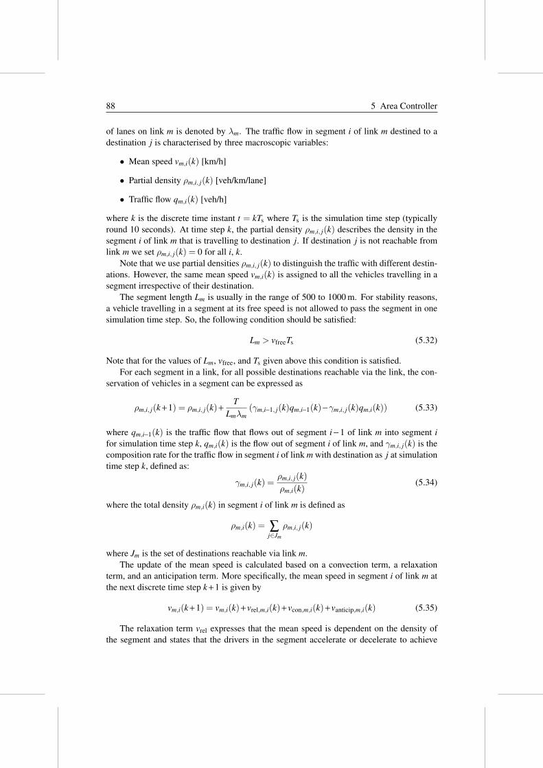
88 5 Area Controller
of lanes on link m is denoted by λm. The traffic flow in segment i of link m destined to adestination j is characterised by three macroscopic variables:
• Mean speed vm,i(k) [km/h]
• Partial density ρm,i, j(k) [veh/km/lane]
• Traffic flow qm,i(k) [veh/h]
where k is the discrete time instant t = kTs where Ts is the simulation time step (typicallyround 10 seconds). At time step k, the partial density ρm,i, j(k) describes the density in thesegment i of link m that is travelling to destination j. If destination j is not reachable fromlink m we set ρm,i, j(k) = 0 for all i, k.
Note that we use partial densities ρm,i, j(k) to distinguish the traffic with different destin-ations. However, the same mean speed vm,i(k) is assigned to all the vehicles travelling in asegment irrespective of their destination.
The segment length Lm is usually in the range of 500 to 1000 m. For stability reasons,a vehicle travelling in a segment at its free speed is not allowed to pass the segment in onesimulation time step. So, the following condition should be satisfied:
Lm > vfreeTs (5.32)
Note that for the values of Lm, vfree, and Ts given above this condition is satisfied.For each segment in a link, for all possible destinations reachable via the link, the con-
servation of vehicles in a segment can be expressed as
ρm,i, j(k + 1) = ρm,i, j(k)+T
Lmλm
(γm,i−1, j(k)qm,i−1(k)−γm,i, j(k)qm,i(k)) (5.33)
where qm,i−1(k) is the traffic flow that flows out of segment i − 1 of link m into segment i
for simulation time step k, qm,i(k) is the flow out of segment i of link m, and γm,i, j(k) is thecomposition rate for the traffic flow in segment i of link m with destination as j at simulationtime step k, defined as:
γm,i, j(k) =ρm,i, j(k)
ρm,i(k)(5.34)
where the total density ρm,i(k) in segment i of link m is defined as
ρm,i(k) = ∑j∈Jm
ρm,i, j(k)
where Jm is the set of destinations reachable via link m.The update of the mean speed is calculated based on a convection term, a relaxation
term, and an anticipation term. More specifically, the mean speed in segment i of link m atthe next discrete time step k + 1 is given by
vm,i(k + 1) = vm,i(k)+ vrel,m,i(k)+ vcon,m,i(k)+ vanticip,m,i(k) (5.35)
The relaxation term vrel expresses that the mean speed is dependent on the density ofthe segment and states that the drivers in the segment accelerate or decelerate to achieve

5.4 Optimal routing for IVHS using a macroscopic traffic flow model 89
a desired equilibrium speed V (ρm,i(k)). The relaxation term is directly proportional to thedifference between the actual mean speed and V (ρm,i(k)) and can be expressed as:
vrel,m,i(k) =Ts
τ(V (ρm,i(k))− vm,i(k)) (5.36)
where τ is related to the driver’s response time and where V (ρm,i(k) can be derived eitherfor human drivers or for IVs. For human drivers a typical value for τ is 18 s [90]. For IVsthis value will be much lower, e.g., 8 s. For human drivers, V (ρm,i(k) is given by (cf. 5.26)
V (ρm,i(k)) = vfree,m exp[
−1
am
(
ρm,i(k)
ρcrit,m
)am]
(5.37)
where am is a model parameter for the specific link m, vfree,m is the free-flow speed for linkm, and ρcrit,m is the critical density at which the traffic flow becomes maximal.The expression of V (ρm,i(k) for IVs is given by (cf. (5.29)):
V (ρm,i(k)) =
{
vfree, if ρm,i(k) ≤ ρACC,crit,m
1hdes
(
1ρm,i(k)
− Lveh
)
, if ρm,i(k) > ρACC,crit,m
(5.38)
The convection term vcon is given by:
vcon,m,i(k) =Ts
Lm
vm,i(k)(vm,i−1(k)− vm,i(k)) (5.39)
and accounts for the effect caused by the vehicles entering the segment i from upstreamsegment i − 1 with different mean speed. The larger the deviation, the larger is the effect ofconvection term on the mean speed.
The anticipation term vanticip expresses the change in speed induced by the drivers’ ex-perience of (total) density that prevails in the downstream segment and is given by:
vanticip,m,i(k) = −ηTs
τLm
ρm,i+1(k)−ρm,i(k)
ρm,i(k)+κ(5.40)
where κ and η are model parameters. Typical values are κ=40 veh/km/lane and η=60 km2/h[90] .
The partial traffic flow for each segment can be described as follows:
qm,i, j(k) = ρm,i, j(k)vm,i(k)λm (5.41)
Origin model
Origins receive traffic demand and forward it to the freeway. Origins are modelled using asimple queue model. A queue is formed at origin o when the traffic demand do(k) exceedsthe service rate qo(k) of the origin. The queue length wo, j(k + 1) destined to destination j
at origin o can be determined from the previous queue length and the total demand do(k) attime step k as follows:
wo, j(k + 1) = wo, j(k)+ Tsγo, j(k)(do(k)− qo(k)) (5.42)

90 5 Area Controller
with γo, j(k) is the fraction of the demand travelling to destination j from origin o. Theoutflow or service rate at origin qo(k) is taken to be the minimum of the number of vehiclesthat want to enter (i.e., total demand at time instant k plus the total number of vehicles inthe partial queues) and the number of vehicles that are actually allowed to enter due to theavailability of space. The outflow can be expressed as:
qo(k) = min[
do(k)+wo(k)
Ts, Qcap,o min
(
1,ρmax −ρµ,1(k)
ρmax −ρcrit,µ
)]
(5.43)
where Qcap,o is the capacity (veh/h) of the origin o under free-flow conditions, ρmax is themaximum density of a segment, and µ is the index of the link to which the origin is connec-ted.
Node model
The node model describes how the traffic should be routed among the set of entering andleaving links of a node. For a given node n, let In denote the set of input links, and let On
denote the set of output links. The traffic flow Qn, j(k) with destination j that enters the noden at simulation step k is distributed to the output links according to
Qn, j(k) = ∑µ∈In
qµ,Nµ(k)γµ,Nµ, j(k) (5.44)
qn,m,out(k) = ∑j∈Jm
βn,m, j(k)Qn, j(k) (5.45)
where qµ,Nµ(k) is the flow leaving the last segment of link µ, βn,m, j(k) is the splitting rate
in node n that is defined as the fraction of the traffic flow heading towards destination j thatleaves node n via output link m, Jm is the set of destinations that are reachable through linkm, and qn,m,out(k) is the total traffic flow that leaves node n via output link m at simulationstep k.
The composition rate γn,m,out, j(k) of the traffic flow out of node n into link m is givenby:
γn,m,out, j(k) =βn,m, j(k)Qn, j(k)
qm,out(k)(5.46)
Downstream density
Consider a node n with input link m ∈ In. Note that the anticipation term (5.40) of the speedupdate equation for segment i of link m contains the downstream density ρm,i+1(k). Hence,we also need an expression for the downstream density for the last segment (segment Nm)of link m. To this aim we introduce a virtual segment Nm +1 at the end of link m as shown inFigure 5.8, and we capture the effect of the downstream density of the output links leavingnode n by the following expression:
ρm,Nm+1(k) =
∑µ∈Onρ2
µ,1(k)
∑µ∈Onρµ,1(k)
(5.47)
where ρµ,1(k) is the density of the first segment of output link µ.

5.4 Optimal routing for IVHS using a macroscopic traffic flow model 91
2 segment
link m
2segmentsegment 1
segment 1 segment
segment m
m
virtual segment m+1
link m
N
NN
Figure 5.8: The first segments of the outgoing links from a node are aggregated into a
virtual segment to provide a virtual downstream density ρm,Nm+1(k)
1 2segmentsegment segment m
virtual segment 0
link m
link m
N
1 2segmentsegment segment mN
Figure 5.9: The last segments of the incoming links are aggregated into a virtual segment
to provide a virtual upstream speed vm,0(k)
Upstream speed
Similarly as above, when a node n has many input links (junction node) as shown in Figure5.9, then the downstream speed for the first segment i = 1 of an outgoing link required inthe convection term (5.39) is captured by adding a virtual segment at the beginning of thelink and by setting
vm,0(k) =∑µ∈Invµ,Nµ
(k)qµ,Nµ(k)
∑µ∈In qµ,Nµ(k)
(5.48)
where Nµ is the index of the last of last segment of link µ.
Extensions
Hegyi et al. [64, 67] have extended the METANET model to include traffic control meas-ures such as dynamic speed limits, and mainstream metering, to account for anticipationbehaviour of drivers to varying downstream densities, and to model main-stream origins.

92 5 Area Controller
model
optimisation
prediction
actionscontrol
objective,constraints
systeminputs
control
MPC controller
measurements
Figure 5.10: Schematic view of the MPC structure.
These extensions can also be integrated in the proposed METANET-like traffic flow modelfor IVHS.
5.4.4 Model predictive route choice control
Now we use the model of the previous subsection to derive a model-based predictive controlapproach that can be used by the area controllers to determine the optimal splitting rates.
More specifically, we adopt the model predictive control (MPC) scheme [30, 101] (seeFigure 5.10). In the MPC control scheme a discrete-time model is used to predict the futurebehaviour of the process, and the MPC controller uses (numerical) optimisation to determ-ine the control signals that result in an optimal process behaviour over a given predictionhorizon. The resulting optimal control inputs are applied using a rolling horizon scheme.At each control step k the state of the traffic system is measured or estimated, and an op-timisation is performed over the prediction horizon [kT,(k + Np)T ] to determine the optimalcontrol inputs, where Np is the prediction horizon. Only the first value of the resulting con-trol signal (the control signal for time step k) is then applied to the process. At the nextcontrol step k + 1 this procedure is repeated.
To reduce the computational complexity and to improve stability often a control horizonNc (≤ Np) is introduced in MPC, and after the control horizon has been passed the controlsignal is taken to be constant. So there are two loops: the rolling horizon loop and theoptimisation loop inside the controller. The loop inside the controller of Figure 5.10 isexecuted as many times as needed to find the optimal control signals at control step k, for thegiven Np, Nc, traffic state, and expected demands. The loop connecting the controller and thetraffic system is performed once for each control step k and provides the state feedback to thecontroller. This feedback is necessary to correct for (the ever present) prediction errors, andto provide disturbance rejection (compensation for unexpected traffic demand variations).The advantage of this rolling horizon approach is that it results in an on-line adaptive controlscheme that allows us to take changes in the system or in the system parameters into accountby regularly updating the model of the system.
For our case the control variables in this set-up are the splitting rates at the nodes withmore than one outgoing link (and if speed limits are included, also these speed limits).The optimisation signals include the control variables as well as the state variables of themacroscopic METANET-like traffic flow model for IVHS derived above.
One can also include various constraints such as maximal flows on certain links, max-

5.4 Optimal routing for IVHS using a macroscopic traffic flow model 93
imal speeds (in case dynamic speed limits are used), maximal travel times for selectedorigin-destination pairs, etc. Moreover, there is a physical constraint that for a given nodethe sum of the splitting rates should be equal to 1:
∑m∈On
∑j∈Jm
βn,m, j(k) = 1 (5.49)
for all n, k.A typical objective function to be used is the total time spent (TTS) by all the vehicles
in the network. This includes both the time spent travelling through the network and thetime spent waiting in the queues, if any. So at time step k we get the following expressionfor the total time spent in the period [kT,(k + Np)T ]:
JTTS(k) =Np−1
∑j=0
(
∑(m,i)∈L ls
ρm,i(k + j)Lmλm + ∑(o, j)∈Ood
wo, j(k + j)
)
Ts (5.50)
where L ls is the set of all link-segment index pairs (m, i) of the network, and O od the set ofall origin-destination pairs (o, j). Note that in (5.50) the expression between the bracketsgives the total number of vehicles present in the links and queues of the network at time stepk + j. This value is multiplied by the simulation time step Ts and summed over the discretetime steps to obtain the total time spent.
Minimising JTTS then results in a nonlinear nonconvex optimisation problem with real-valued variables. In general this is an NP-hard problem [53] just like the original routechoice problem. In fact with 5.50, we now have an optimisation problem with real-valuedvariables, which offers a major advantage compared to the mixed-integer optimisation ofthe original route choice problem, since due to the smoothness of the objective function,the real-valued optimisation will require a lower computational effort to find (sub)optimalsolutions.
To solve the nonlinear optimisation problem we can use a global or a multi-start localoptimisation method [118] such as multi-start sequential quadratic programming, patternsearch, genetic algorithms, or simulated annealing.
5.4.5 Case study
In this subsection we present a simple case study involving a basic set-up to illustrate thearea-level control approach for IVHS proposed in this section. First, we will describe theset-up and the details of the scenario used for our simulations. Next, we will discuss andanalyse the obtained results.
Scenario
We consider a simple network of highways with one origin o1 and two destinations d1, d2,and three internal nodes v1, v2, and v3 (see Figure 5.11). Note that this example is similarto the one of Section 5.3.8. However, due to the different type of model used, the waythe case study is specified will differ. The network of Figure 5.11 consists of three links10
10In contrast to the example of Section 5.3.8 we now explicitly consider these origin and destination links inorder to account for the effect of the boundary conditions.
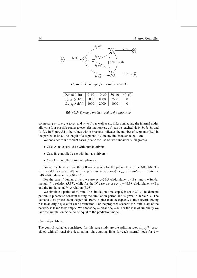
94 5 Area Controller
(2)
(5)
(1)
(3)
(2)
(1)l9
(6)
(10)
(7)
l1
l2
l3
l4
l5
l6
l8
l7
o1
d1
d2
v1
v2
v3
Figure 5.11: Set-up of case study network
Period (min) 0–10 10–30 30–40 40–60Do1,d1
(veh/h) 5000 8000 2500 0Do1,d2
(veh/h) 1000 2000 1000 0
Table 5.3: Demand profiles used in the case study
connecting o1 to v1, v2 to d1, and v3 to d2, as well as six links connecting the internal nodesallowing four possible routes to each destination (e.g., d1 can be reached via l2, l3, l4+l9, andl5+l9). In Figure 5.11, the values within brackets indicates the number of segments (Nm) inthe particular link. The length of a segment (Lm) in any link is taken to be 1 km.
We consider four different cases (due to the use of two fundamental diagrams):
• Case A: no control case with human drivers,
• Case B: controlled case with humans drivers,
• Case C: controlled case with platoons.
For all the links we use the following values for the parameters of the METANET(-like) model (see also [90] and the previous subsections): vfree=120 km/h, a = 1.867, κ
=40 veh/km/lane and η=60 km2/h.For the case if human drivers we use ρcrit=33.5 veh/km/lane, τ=18 s, and the funda-
mental V –ρ relation (5.37), while for the IV case we use ρcrit =48.39 veh/km/lane, τ=8 s,and the fundamental V –ρ relation (5.38).
We simulate a period of 60 min. The simulation time step Ts is set to 20 s. The demandpattern is piecewise constant during the simulation period and is given in Table 5.3. Thedemand to be processed in the period [10,30) higher than the capacity of the network, givingrise to an origin queue for each destination. For the proposed scenario the initial state of thenetwork is taken to be empty. We choose Np = 20 and Nc = 6. For the sake of simplicity wetake the simulation model to be equal to the prediction model.
Control problem
The control variables considered for this case study are the splitting rates βn,m, j(k) asso-ciated with all reachable destinations via outgoing links for each internal node for k =

5.5 Interface between area and roadside controllers 95
0,1, . . . ,Nsim − 1 where Nsim = 180 is the total number of simulation steps (of length Ts
= 20 s) within the entire simulation period of 60 min.Since it makes no sense to send vehicles reaching node v2 and going to destination
1, towards link l8 we set βv2,l6,1(k) = 1 and βv2,l8,1(k) = 0 for all k. Likewise, we setβv2,l6,2(k) = 0 and βv2,l8,2(k) = 1 for all k. For node v3 we have similar expressions:βv3,l7,1(k) = 0 and βv3,l9,1(k) = 1, βv3,l7,2(k) = 1, βv3,l9,2(k) = 0 for all k. So in fact theoptimisation variables are βv1,m, j(k) for m = l2, l3, l4, l5 and j = 1,2.
We have the following constraints (cf. (5.49)):
βv1,l2, j(k)+βv1,l3, j(k)+βv1,l4, j(k)+βv1,l5, j(k) = 1
for j = 1,2 and for all k.The goal of our area controller is to improve the traffic performance. The objective
that we consider for our case study is minimisation of the total time spent (TTS) by allthe vehicles in the network using routing as the control measure. The TTS for the entiresimulation period can be expressed as (cf. (5.50)):
JTTS,sim =Nsim−1
∑k=0
(
∑(m,i)∈L ls
ρm,i(k)Lmλm + ∑(o, j)∈Ood
wo, j(k)
)
Ts (5.51)
where L ls is the set of all link-segment index pairs (m, i) of the network, and O od the set ofall origin-destination pairs (o, j).
Results and analysis
The results of the numerical experiments are listed in Table 5.4.In case of no control (Cases A and B), the capacities of the direct links l1, l2, l3, and l4
are consumed up to their maximum while the links l8 and l9 are not used due to the fact thatall vehicles and platoons want to take the shortest routes. At the point when the demandexceeds the maximum capacity of the links, origin queues are formed. As the simulationadvances, the queue length increases with time, thus leading to a huge total time spent.
For the controlled cases (Cases B and C) the area controller assigns the splitting ratesat the internal node v1 and routes the traffic flow (human drivers or platoons) in a system-optimum manner such that the traffic performance is improved. When platoons of ACC-equipped vehicles are deployed in the traffic system, the traffic performance is improvedmore than the human drivers case. For these cases we have used the SQP function SNOPT,implemented via the function snopt of the Matlab Tomlab toolbox, to compute the optimalsplitting rates. Compared to Case A this results in a performance improvement of about 3 %for Case B and of about 46 % for Case C.
5.5 Interface between area and roadside controllers
The area controllers will provide flow targets to the roadside controllers (e.g., using theapproaches proposed in Sections 5.3, and 5.4), which then have to control the platoons thatare under their supervision in such a way that these targets are met as well as possible. In our
10On a 1 GHz Athlon 64 X2 Dual Core 3800+ processor with 3 GB of RAM.

96 5 Area Controller
Case JTTS,sim improvement(veh.h) (%)
no control (A) 686.28 0 %controlled human 670.91 3 %controlled IVs 366.07 46 %
Table 5.4: Results for the case study. The improvement is expressed with respect to the
no-control case with human drivers.
IVHS framework, the area and roadside controllers use a different level of representationof the traffic. However, consistency between the macroscopic traffic characteristics (suchas flows, splitting rates) and the platoons has to be established to ensure efficiency of theapproach. Hence, our approach requires an interface between these controllers, which isimplemented as follows:
Once the optimal target flows are determined by the area controller, the roadside con-troller has to realise the target flows on each link as well as possible by using the availablecontrol measures such as speed limits, ramp matering, route guidance, and lane control. Inorder to achieve the specified optimal flows on the links, the roadside controller will usea performance criterion based on the minimisation of the difference between the referenceflows and the actual flows. The roadside controller is aware of the complete information ofthe IVs (i.e., position, speed, lane, origin, destination) and hence can determine the actualflow xl,o,d(k) on each link l for all (o,d) ∈ O ×D . At each control step k, the roadside con-troller will be updated with this flow information. The corresponding performance functionJperf used by the roadside controller is then given by
Jperf =Kend−1
∑k=0
∑(o,d)∈O×D
∑l∈Lo,d
(xoptl,o,d(k)− xl,o,d(k))
2 (5.52)
where xoptl,o,d(k) is the optimal flow specified by the area controller for link l in (o,d)∈ O ×D
for all k.At the nodes, the roadside controller will additionally provide routing instructions for
every platoon on the stretch under its supervision. The roadside controller will give theserouting instructions by taking account of platoons’ destinations and also the target flows onthe adjacent highways. If necessary, the node controller can provide commands for platoonsplits and merges, and determine new platoon compositions and platoon lengths.
5.6 Summary
We have considered the optimal route guidance problem for IVHS. Since the resulting op-timisation problem is a nonlinear mixed-integer optimisation problem that in general is tooinvolved for on-line, real-time implementation, we have explored approximations resultingin simplified but fast simulation models that yield mixed-integer linear or nonlinear real-
valued optimisation problems, for both of which efficient solvers exist.

5.6 Summary 97
The first approach was based on a simplified model that describes the movement of theplatoons in the network via flows. We have shown that using this model the optimal routechoice control problem can be approximated by a linear or a mixed-integer linear problem.With a case study we have illustrated that the resulting approach can offer a balanced trade-off between computational efficiency and optimality.
In the second approach we have developed a new model to describe the flow of platoonsin the IVHS based on the macroscopic METANET traffic flow model, which has been adap-ted to fit the case of platoons of intelligent vehicles equipped with Adaptive Cruise Control(ACC). This model has subsequently been used in a model predictive control approach fordetermining optimal splitting rates of the platoon flows at the nodes in the network. Lower-level roadside controller can then translate these splitting rates into actual route instructionsfor the platoons. The proposed approach has also been illustrated via a simple case study.
In our future research, we will compare these two approaches (with a microscopic modelas simulation model), consider additional case studies, and assess the performance improve-ment of the proposed approaches with respect to an approach based on mixed-integer op-timisation for the original route choice problem. We will also investigate the coordinationand mutual interaction between various area controllers and between the area controllersand the roadside controllers.

98 5 Area Controller

Chapter 6
Traffic Management with
Semi-Autonomous Intelligent
Vehicles1
In this chapter, we deal with traffic congestion problems by using an intermediate approachwhich deploys a system that can be conceptually placed between the conventional trafficsystems and fully automated IVHS that was discussed in the previous chapters. More spe-cifically, human-driven vehicles in the conventional traffic systems are equipped with ad-vanced driver assistance systems that can improve the traffic flow and that can also supportthe existing traffic control measures. We will in particular focus on how an infrastructure-based traffic controller can determine appropriate dynamic speed limits for such an inter-mediate traffic systems.
6.1 Introduction
The ever-increasing demand for mobility and transportation results in a growing traffic con-gestion problem. One of the promising approaches to reduce the frequency and impact oftraffic jams is the optimal and efficient usage of the existing system. This approach willresult in integrated traffic management and control systems that incorporate intelligencein both the roadside infrastructure and in the vehicles, and that are commonly called In-telligent Vehicle Highway Systems (IVHS). Vehicles in an IVHS are arranged in closelyspaced groups called platoons. In the platooning approach cars travel on the highway inplatoons with small distances (e.g., 2 m) between vehicles within the platoon, and muchlarger distances (e.g., 30–60 m) between different platoons. High speeds and short intrapla-toon spacings allow more vehicles to be accommodated on the network, which substantiallyincreases the maximal traffic flows [149].
In this chapter we discuss a traffic control approach that is situated in between the cur-rent situation with human drivers and no direct interaction between the roadside control
1This chapter is based on the MSc thesis of Mernout Burger [29].
99

100 6 Semi-Autonomous Intelligent Vehicles
model
optimization
prediction
actionscontrol
objective,constraints
systeminputs
control
MPC controller
measurements
(a) The MPC control loop
x^
u
predicted states
computed control inputs
control horizonprediction horizon
k k+1 k+N
futurepast
current state
k+N pc...
(b) Prediction and control horizon in MPC
Figure 6.1: Schematic representation of MPC
system and the vehicles, and the future IVHS-based situation with fully controlled intel-ligent vehicles. In particular, we consider a situation in which intelligent vehicles drivenby human drivers and equipped with ISA interact with the roadside controller (advisoryISA). Therefore, we call this type of vehicles semi-autonomous, as the human driver is stillin control. We will investigate the possibility of using the semi-autonomous vehicles fortraffic control, and design a traffic control method for this traffic system.
In Section 6.2.1, we present the strategy behind the model-based predictive control(MPC) approach. Later in Section 6.3, we propose an MPC approach to determine ap-propriate dynamic speed limits for the semi-autonomous traffic system. In Section 6.4, wediscuss a model that could be used for simulation purposes. We also present the details ofplugins that will be used as an interface between the simulation package Paramics and theMatlab engine where the traffic controller will be implemented. In Section 6.6, we applythe proposed approach to a case study based on simulations and we highlight the potentialeffects of the semi-autonomous systems on the traffic performance.
6.2 Preliminaries
6.2.1 Model Predictive Control (MPC)
Model Predictive Control (MPC) [30, 101] has originated in the process industry and it hasalready been successfully implemented in many industrial applications. MPC makes useof discrete-time models. Let Tctrl be the control sampling interval, i.e., the time intervalbetween two updates of the control signal settings. At each time step k (correspondingto time t = kTctrl), the MPC controller first measures or determines the current state x(k)of the system. Next, the controller uses (on-line) optimisation and an explicit predictionmodel to determine the optimal values for the control measures over a given predictionperiod determined by the control horizon Np (see Figure 6.1(b)). In order to reduce thecomputational complexity of the problem, one often introduces a constraint of the formu(k + j) = u(k + j − 1) for j = Nc, . . . ,Np − 1, where Nc is called the control horizon.
The optimal control inputs are then applied to the system in a receding horizon approachas follows. At each control step k only the first control sample u∗(k) of the optimal control

6.3 MPC for semi-autonomous traffic 101
sequence u∗(k), . . . ,u∗(k + Nc − 1) is applied to the system. Next, the prediction horizon isshifted one step forward, and the prediction and optimisation procedures over the shiftedhorizon are repeated using new system measurements. This receding horizon approach in-troduces a feedback mechanism, which allows to reduce the effects of possible disturbancesand mismatch errors.
6.2.2 In-vehicle measures
We briefly discuss various in-vehicle technologies that serve as an intermediate in betweenthe current traffic management system and IVHS-based approach. We will consider a trafficsituation where the human-driven vehicles are equipped with ISA.
A standard speed limiter is a system that restricts the speed of the vehicle when the drivertries to exceed the maximum allowed driving speed. When the speed limiter is incorpor-ated with the intelligence to adjust the maximum driving speed to the speed limit specifiedby the roadside infrastructure or to the prevailing location-based legal speed limit, and toprovide feedback to the driver when that speed limit is exceeded, then we get the techno-logy called Intelligent Speed Adaptation (ISA) [24, 39]. Based on the way the system reactson exceeding the legal speed limit, advisory systems only give a warning (visually or viasound). Systems that decrease the possibility of speeding by increasing the resistance of theaccelerator pedal, called an active acceleration pedal, and systems that do not allow a driverto exceed the speed limit (possibly also by limiting the throttle) can either be voluntary ormandatory (also called optional and obligatory). The voluntary system can be turned on andoff by the user, the mandatory system is always on.
6.3 MPC for semi-autonomous traffic
Now, we focus on how MPC can be applied for speed control of the semi-autonomous trafficsystems. In this section, we will use a macroscopic model (METANET) for predictions andwill use microscopic model Paramics to represent the real-life traffic situation.
6.3.1 Prediction model
There exists a wide range of traffic models [43]. Microscopic models are more suitablefor simulation purposes and, for off-line evaluation of developed control strategies than foron-line model-based control. In principle, microscopic traffic simulation models are usuallynot suited as MPC prediction model. An important factor that determines the choice of theprediction model to be used in MPC is the trade-off between accuracy and computationalcomplexity. The prediction model needs to be able to simulate the entire network muchfaster than real-time in order to be able to predict the future states of the network in time.For the prediction of the future states of the traffic network with semi-autonomous vehicles,we use the macroscopic traffic flow model METANET [90, 91, 104, 115].
In the METANET model, the traffic network is represented as a directed graph withthe links corresponding to the highway stretches. In this section, we will consider a net-work with one origin and one destination. Hence, we can use a destination-independentMETANET model. The basic METANET model consists of link equations and node equa-tions. A detailed description of destination-oriented METANET model was discussed in

102 6 Semi-Autonomous Intelligent Vehicles
direction of traffic flow downstream
ρ18(k)ρ1(k) ρdown(k)ρi−1(k) ρi+1(k)ρi(k)ρup(k)
segment segmentupstream
v18(k)v1(k) vdown(k)vi−1(k) vi+1(k)vi(k)vup(k)
Figure 6.2: State variables of the segmented road. Since we will work with a link, the link
variable m is left out.
Chapter 5 in Section 5.4.3. Each highway link m is divided into Ns,m segments of equallength Lm, with λm the number of lanes on link m. For illustration, we consider a 10 kilo-metres stretch of a highway as shown in Figure 6.2. The highway is divided into 20 segmentsof 500 metres length, with two lanes at each segment. On all segments, the density and meanspeed are measured. The first and last segments are used to describe boundary values, andthe other 18 segments are used to control the traffic. In Figure 6.2 the uncontrolled parts areshown in grey.
Each segment i of highway link m is now characterised by
• Mean speed vm,i(k) [km/h]
• Traffic density ρm,i(k) [veh/km/lane]
• Traffic flow qm,i(k) [veh/h]
where k is the discrete time instant t = kT , where T is the simulation time step, typically 10seconds for a segment length Lm of 500 metres.
Since we are working with only one link, also the link variable m can be left out of theequations. The extension for variable speed limits is used to model the controlled segments.The update equations for the state variables for a road segment then become
ρi(k + 1) = ρi(k)+T
λL(qi−1(k)− qi(k))
= ρi(k)+T
L(ρi−1(k)vi−1(k)−ρi(k)vi(k))
vi(k + 1) = max[
vi(k)+T
τ(vdes,i(k)− vi(k))
+T
Lvi(k)(vi−1(k)− vi(k))−
ηi(k)T
τL
ρi+1(k)−ρi(k)
ρi(k)+κ, vmin
]
(6.1)
where κ and η are model parameters, vmin is minimum allowed mean speed (typical valueis 4 km/h) and vdes,i(k) is the desired mean speed of the vehicles. Let us now considerthe (equilibrium) relation between the speed v and the density ρ. When the density on theroad is very low and the average distance headway is large, the drivers travel at their desiredspeed. This is called free-flow driving. As the density starts to increase due to the increasingdemand, the vehicles will start to reduce their speed slightly and follow their predecessorwhile maintaining a safe time headway. Once the critical density (i.e., the density at whichthe capacity of the network is being utilised at its maximum) is reached, the speed starts todecrease significantly resulting in a traffic jam. When the density is at its maximum (ρmax),

6.3 MPC for semi-autonomous traffic 103
the vehicle speed drops to almost zero. The (equilibrium) relation between the speed v andthe density ρ can be modelled as [102]:
vdes,i(k) = vfree exp[
−1a
(
ρi(k)
ρcrit
)a]
(6.2)
where ρcrit is the critical density, vfree is the free-flow speed, and a is a model parameter.Hegyi et al. [66] extended this model in order to include the effects of variable speed
limits and to account for different reactions of drivers to varying downstream densities. Theeffect of variable speed limits is included by adjusting the desired speed equation vdes,i(k)to take the minimum of the density based free-flow speed, or the given variable speed limitvctrl,i(k) adjusted by a compliance factor 1 + α to indicate the noncompliance to the speedlimit. Equation (6.2) then becomes
vdes,i(k) = min(
vfree exp[
−1a
(
ρi(k)
ρcrit
)a]
, (1 +α)vctrl,i(k)
)
(6.3)
In order to include the different reactions of drivers to the downstream density the globalvariable η in (6.1) should be replaced by the segment, and time dependent variable
ηi(k) =
{
ηhigh if ρi+1(k) ≥ ρi(k)
ηlow if ρi+1(k) < ρi(k)
Origins are modelled using queues. The length of the queue wo(k) is given by
wo(k + 1) = wo(k)+ T (do(k)− qo(k)) (6.4)
where do(k) is the demand and qo(k) is the outflow at time k. The outflow is the minimumof the demand and the maximal flow that can enter the motorway:
qo(k) = min[
do(k)+wo(k)
T, Qo
ρmax −ρµ,1(k)
ρmax −ρcrit,µ
]
(6.5)
where Qo is the on-ramp capacity under free-flow conditions, ρmax is the maximum densityon the motorway, and µ the index of the link under consideration.
The boundary states are also updated, using the state of the boundary segment of interestfor the unknown states of the adjacent segments. This results in reduced update equationsfor the boundary segments, given by
vup(k + 1) = max[
vi(k)+T
τ(vdes,up(k)− vup(k))−
ηdes,up(k)T
τL
ρ1(k)−ρup(k)
ρup(k)+κ,vmin
]
ρup(k + 1) =qup(k + 1)
λvup(k + 1)=
qup(k)
λvup(k + 1)= ρup(k)
vup(k)
vup(k + 1)
vdown(k + 1) = max[
vdown(k)+T
τ(vdes,up(k)− vup)+
T
Lvdown(k)(v18(k)− vdown(k)) ,vmin
]
ρdown(k + 1) = ρdown(k)+T
L(ρdown−1(k)vdown−1(k)−ρdown(k)vdown(k)) (6.6)
where vdes,up and vdes,down are calculated as in (6.3), where the first term is used, since thereare no speed limits on the boundary segments. The parameter value ηup can be determined

104 6 Semi-Autonomous Intelligent Vehicles
as in (6.3.1). In the update for the upstream density ρup(k+1), we have assumed a constantflow, so qup(k+1)=qup(k). Also, v18(k) is the mean speed on segment 18. The parametersof the METANET model (τ , α, κ, kcrit, vfree, a, ηhigh and ηlow) need to be determined bycalibration as described in Section 6.6.
6.3.2 Performance criteria and constraints
Possible performance criteria Jperf(k) for MPC are the total time spent in a traffic network,the total throughput, the total fuel consumption, safety, or a combination of these, all evalu-ated over the time period [kTctrl,(k +Np)Tctrl). Moreover, in order to prevent oscillations andfrequent shifting in the control signals, one often adds a penalty on variations in the controlsignal u in both time and space, which results in the total performance function
T T S = Jperf(k) + λ1
Nc−1
∑j=0
Ns
∑i=1
‖ui(k + j)− ui(k + j − 1)‖2
+ λ2
Nc−1
∑j=0
Ns−1
∑i=1
‖ui+1(k + j)− ui(k + j)‖2 , (6.7)
at control step k, where λ1,λ2 > 0 are weighting factors, and ui(k) is the control signal insegment i at time step k.
The MPC controller also explicitly takes into account operational constraints such asminimum and maximum speeds, etc.
6.4 Simulation model - Paramics
Paramics is a suite of software tools used to model the movement and behaviour of indi-vidual vehicles on urban roads and highway networks. It uses microscopic characteristicssuch as speed, position, etc, to simulate the interaction between vehicles and the road net-work. We are interested in this software program, mainly due to the possibility to add extrafunctionalities by creating plugins.
During a simulation, the acceleration for every vehicle in the network is calculated,based on the speed limit, headway, speeds of vehicles nearby, and the desired free-flowspeed of the vehicle. For this research, we will change the speed limits dynamically, andimplement ISA-equipped vehicle behaviour in Paramics, by changing the desired free-flowspeed of vehicles, which will be discussed in Section 6.5.
The longitudinal aspects of the driver tasks can be classified as free-flow, car-following,and stop-and-go behaviour. In free-flow behaviour, the vehicles can travel at their desiredspeed (corresponding to the speed limit, e.g, 120 km/h). As the traffic demand increases,the vehicles start to follow their predecessors on the same lane at closer distances and atreduced speeds (50–80 km/h). Once the capacity of the highway is being utilised at itsmaximum, the vehicles move with stop-and-go movements (0–40 km/h). There are twoimportant microscopic submodels used in Paramics, namely for the car-following behaviourand the way the desired headway is determined per vehicle.

6.4 Simulation model - Paramics 105
l
l
l
Vl −1l
V
g
s
t
Figure 6.3: Representation of target points for car-following in Paramics
Car-following behaviour
The car-following behaviour is split into three modes; braking, cruising, and accelerating.For all modes, the concept of a target point is used. For vehicle l, this target point sl iscalculated as
sl = hdesvl−1 (6.8)
where sl is the spacing, hdes is the desired headway and vl−1 is the speed of the precedingvehicle. The situation is shown in Figure 6.3. In order to account for the reaction time ofhuman drivers the speed vl−1 used is actually the speed of the preceding vehicle some timein the past. In order to make the vehicles reach the desired headway faster, an adjusted targetpoint tl is used, calculated by
tl =s2
l
gl
where gl is the current distance between the vehicles. Note that this indeed will speed upreaching the target point dependent on the desired headway and vehicle speed, since
tl < sl if gl > sl
tl = sl if gl = sl
tl > sl if gl < sl
and using tl as the desired spacing the difference |(tl − gl)| between the current spacing anddesired spacing will always be bigger or equal than when we use sl as desired spacing.
The cruising mode is split up into three separate regions, called A, B ,and C. The brakingmode will be called region D, and the acceleration mode is region E. The characteristics ofthe regions are
• Region A: the following vehicle has overshot the target point (the spacing is less thanthe target value), and an attempt is made to achieve the target speed as quickly aspossible.
• Region B: the leading vehicle is pulling away from the following vehicle.
• Region C: the vehicles are at a constant separation or coming closer together.
• Region D: the leading vehicle is decelerating with a value above a certain thresholdso that, the following vehicle will notice the leading vehicle is braking. The followingvehicle will start to brake as well.

106 6 Semi-Autonomous Intelligent Vehicles
• Region E: the leading vehicle is accelerating with a value above a certain threshold,the following vehicle will notice the leading vehicle is accelerating. The followingvehicle will start to accelerate as well.
The accelerations for the following vehicle for the different regions are given by
aA = k1∆v + k2gl − tl
gl
aB = k1∆v + k3gl − tl
tl
aC = c −(∆v)2
gl − tl
aD = amin
aE = amax
where k1 = 1.0 [s−2], k2 = 1.0 [s−2], k3 = 0.005 [s−2], ∆v = vl−1 − vl , c the bunching ac-celeration to bring the vehicles together rapidly, and amin and amax, are the minimum andmaximum acceleration of the vehicle respectively.
Headway of vehicles
The desired headway is dependent on the type of vehicle, the situation in the network, andthe driver behaviour. It is based on an average headway, which can be set for the simula-tion. Each vehicle has several multiplication factors, which together determine the desiredheadway of the individual vehicle. Each vehicle type has a type-dependent multiplicationfactor. Using this factor, we can, e.g., include the larger headway a heavy goods truck needscompared to a car, since it can decelerate less strongly. Two important driver characteristicsused in Paramics for manipulating the driver behaviour are the aggressiveness and aware-ness. Aggressiveness is used to influence the headway everywhere in the network. Themultiplication factor for aggressiveness is calculated using
Fag =
36 − 5θag
16, θag ≤ 4
12 −θag
8, θag > 4
(6.9)
where θag is the assigned level of aggressiveness of the driver, indicated by a value between1 and 8. A lower value for θag means that the driver is less aggressive, and will have alarger desired headway. The awareness factor is used to calculate the desired headwaywhen a vehicle is near a lane drop. It is used to simulate to what extent a driver will keepdistance to the vehicle in front in order to let other vehicles merge into the other lane. Thismultiplication factor is given by
Faw =
θaw + 48
, θaw ≤ 4
θaw − 3, θaw > 4(6.10)
where θaw is the awareness factor of the driver, indicated by a value between 1 and 8. Ahigher value means that the driver is more aware of other vehicles wanting to get onto thelane, and the driver will have a larger desired headway near lane drops.

6.5 Coupling Paramics and Matlab 107
6.5 Coupling Paramics and Matlab
Since there is no existing interface between the Paramics and Matlab, we will create aplug-in to simulate the behaviour of IV-based vehicles. We will develop plug-ins for thepartially automated vehicles to capture their reaction to the control measures. The firstplugin is created to be able to measure mean speeds, densities, flows, and the number ofpassing vehicles on a road segment, and to send this data to a Matlab engine. A trafficcontroller created in Matlab can then be used to calculate control actions for the trafficnetwork in Paramics. The second plugin is created to change the behaviour of the vehiclesin Paramics. Using this plugin, ISA-equipped vehicles can be used in the simulation. Alsothe vehicle behaviour when using unenforced and enforced speed limits can be influencedby this plugin.
6.5.1 Interface plugin
The Interface plugin can be used as a stand-alone plugin and is created in Paramics. Itis created to measure data in Paramics, and also to use it to control the simulated trafficin Paramics, via a controller implemented in Matlab. The traffic measurements needed tocalculate the control actions are obtained from Paramics. These control actions will then besent back to Paramics to simulate the response of traffic on these control actions.
Measurement data
The plugin makes use of data collected by detectors. When a vehicle passes a detector, itwill be counted, and its speed will be used to calculate the mean speed on the segment thedetector is on. Therefore, in order to be able to use the Interface plugin, some detectorsshould be placed in the Paramics project and the details on how to do this can be found inthe Paramics Modeller manual. Every simulated minute the plugin will determine the valuesof the measurements in Paramics, and send this data to the Matlab engine. When the simu-lation is finished, the data will be stored in three different mat-files namely detector.mat,control.mat and odmatrix.mat. These mat-files can be found in the same directory fromwhere we started the Paramics program.
The file detector.mat contains a three-dimensional matrix representing simulatedminute, detector number, and index number of the detector data. The data obtained fromthe detectors is stored in an array with index numbers indicating simulation time, estimatedspace-mean density, time-mean density, approximated space-mean density, average flow,estimated space-mean speed, time-mean speed, approximated space-mean speed, vehiclecount (minute) and vehicle count (total). The approximated values are calculated by de-termining the values (e.g., space mean density) of a segment at every second, sum thesevalues for one minute, and determine the average value for that minute. The estimatedvalues are determined using the basic macroscopic traffic characteristics equations. For ex-ample, detector(20,7,5) will give the flow (index 5) at detector 7 for the 20th simulatedminute.
The file control.mat contains a matrix representing simulatedminute, controlled segment number, and control action number. The control action data mat-

108 6 Semi-Autonomous Intelligent Vehicles
Figure 6.4: The Interface plugin dialog box
rix contains the dynamic speed limits (ctrnr=1), and the dynamic time headways (ctrnr=2)2,for all timesteps at all controlled segments. The plugins are made with more types of intel-ligent vehicles in mind. Another interesting type of intelligent vehicles are ACC equippedvehicles. Besides dynamic speed limits, also the time headway of these vehicles might bechanged in order to improve the network performance. In this way both means speeds anddensities can be influenced, giving the traffic controller an extra degree of freedom. This iswhy the traffic controller is supposed to return both speed limits and time headways.
The file odmatrix.mat contains four-dimensional matrix representing simulatedminute, detector number, origin number, and destination number. The origin-destinationdata array contains the number of vehicles that came from a certain origin, and want to goto a certain destination in the network, counted in the passed simulated minute. The indexnumbers of the origins and destinations correspond to the zone numbers in Paramics.
Interface plugin parameters
Different parameters of the Interface plugin shown in Figure 6.4 are described:
• Log and show measurements: The checkboxes indicate to the plugin whether it shouldlog the measurements in a textfile as data.txt or show the measurements in thereporter window.
• Use the traffic controller: This checkbox tells whether the traffic controller shouldbe called at every simulated minute. When the traffic controller is set to ’true’,the Interface plugin will call an m-file called traffic_controller at every sim-ulated minute. This function can be used as [speedlimitdata headwaydata]=traffic_controller(minute,state), where
– speedlimitdata is a vector containing the dynamic speed limits for the con-trolled segments, in kilometres per hour. These speed limits are the control
2Desired headway control can be used for controlling ACC-equipped vehicles.
6.5 Coupling Paramics and Matlab 109
actions of the controller, which will be applied to the network during the nextsimulation minute.
– headwaydata is a vector containing the dynamic time headways for the con-trolled segments, in seconds. These time headways are the control actions ofthe controller, which will be applied to the network during the next simulationminute.
– minute is the current simulation minute, for which the measurements are taken.
– state is a matrix containing the mean speeds and densities from the measuredsegments. These measurements can be used by the controller to determine itsnext control actions.
• Controller delay [min]/[sec]: This is the amount of minutes plus seconds the pluginwill wait after the start of the calculation of new control values, before the controlactions are applied. The Paramics simulation will wait until the controller is finished.In this way, the time a controller may use to calculate the next control values can betaken into account in the simulation. The value for the minutes is an integer between0 and 10, the value for the seconds is an integer between 0 and 59.
6.5.2 ISA plugin
The ISA plugin is dependent on the Interface plugin, so the Interface plugin should alsobe loaded if one intends to use the ISA plugin. It is created to simulate vehicles equippedwith an ISA system. This is done by giving all vehicles of a certain type (“ISA vehicles”)a compliance factor. First, we motivate the reason for creating this plugin, followed by anexplanation of the parameters of the plugin.
Intended use
We want to investigate the differences in controlling three scenarios, namely traffic drivingwith unenforced speed limits, traffic driving with enforced speed limits, and traffic consist-ing of vehicles equipped with ISA systems. Vehicles equipped with ISA can be modelledusing their free-flow speed distribution. The effects on mean speeds and the speed distribu-tion for vehicles can be modelled by a normal distribution. They are based on research usingISA with an active acceleration pedal [70]. This research was carried out in the city of Lund,Sweden. It covered measurements on main streets and arterial roads. On the main streets,there was no significant difference in speed distribution between vehicles with and withoutactive acceleration pedal. On the arterial roads (with speed limits of 50 and 70 km/h), thestandard deviation of the active acceleration pedal equipped vehicles was about 5.7% of thespeed limit, and without active acceleration pedal it was about 9.9% of the speed limit. Thedecrease in the standard deviation on arterial road is due to the decrease in speed of the fast-est vehicles, but also due to the increase of speed of the slowest vehicles. The mean speed onthe arterial roads is about 110% of the speed limit for vehicles without active accelerationpedal, and about 100% for vehicles with active acceleration pedal. A similar conclusionwas drawn from measurements on a highway in the Netherlands [67]. Here it was foundthat vehicles drive about 10% faster when the speed limits are unenforced, and about 10%too slow when they are enforced.

110 6 Semi-Autonomous Intelligent Vehicles
0 20 40 60 80 100 120 140 160 1800
1
2
3
4
5
6
7
desired free flow speed [km/h]
pro
ba
bili
ty [
%]
unenforced speed limit
intelligent speed adaptation
enforced speed limit
Figure 6.5: Gaussian distributions of the desired free-flow speeds
We assign a compliance factor to every vehicle, based on the distribution belonging toits type. This factor is used to give a vehicle a desired speed, based on the current speedlimit on the road. The calculation for the desired speed thus becomes
vdes,n = αcf,n · vspeedlimit
where, αcf,n respresents the compliance factor of vehicle n and is a Gaussian random num-ber. The used mean value and standard deviation used depend on the scenario that is con-sidered.
In the case of simulating ISA equipped vehicles, a distribution is used with the meanvalue near 1.00, and a small standard deviation. In literature, values are found for thestandard deviation of ISA vehicles [70]. Measurements on arterial roads with speed limitsof 50 and 70 km/h give standard deviations of about 5.7%. Since this article also shows thatthe standard deviation decreases with increasing speeds, and we simulate a highway with aspeed limit of 120 km/h, a standard deviation of 5.0% is used.
Also for the non-ISA vehicles, a compliance factor can be used. For the situation ofunenforced speed limits a Gaussian random number is determined with a mean value near110% of the speed limit, and a larger standard deviation. This value can be found in both[67] and [70]. In the latter article, the standard deviation on the arterial roads is 10.2% at50 km/h and 9.6% at 70 km/h. Here we assume that the standard deviation is 8.0% at 120km/h.
When the speed limits are enforced (e.g. by trajectory control), human drivers tend todrive slower than the speed limit [67], at about 90% of the speed limit. This behaviour canalso be described by using a random compliance factor. The standard deviation is takenequal to the one in the unenforced situation. The probability distribution functions for thethree different scenarios are shown in Figure 6.5. The used speed limit is 120 km/h. Dueto the smaller standard deviation for the ISA equipped vehicles compared to the other twotypes, the chance of having a desired free-flow speed near the mean value becomes bigger,as can be seen by the higher and narrower peak for this type.

6.6 Case study 111
Figure 6.6: The ISA plugin dialog box
ISA plugin parameters
The different parameters of the ISA plugin shown in Figure 6.6 are defined as follows,
• Vehicle numbers: This parameter indicates which vehicle type in Paramics shouldbehave as ISA-equipped vehicles and which vehicles should behave as second-typeand third-type vehicles. The value is an integer between 1 and 10.
• Compliance factor for vehicles: mean and st.dev.: These parameters give the meanvalue and the standard deviation for the compliance factor for ISA-equipped, type 2and type 3 vehicles. The value can be chosen between 0.50 and 1.50.
6.6 Case study
Now we present a simple case study in which the MPC control strategy for the roadsidecontroller layer that has been described in Section 6.3 is applied. First we will describe theset-up of the network, which will be followed by a description of how this network can bemodelled by the METANET model as well as other implementation details. Next, we willdiscuss and analyse the results obtained from the simulations. For our simulations, we willconsider dynamic speed limits as the control measure.
6.6.1 Set-up
The network used for the simulation is similar to the stretch discussed in Figure 6.2 and is atwo-lane highway stretch, with one on-ramp at the end. The stretch consist of 20 segments

112 6 Semi-Autonomous Intelligent Vehicles
������
������
������
������
������
������
���������������������������������������������������������
���������������������������������������������������������
������������
������������
������������
������������
onramp
O1
O2
D1
s1 s2 s3 s19 s20
100 80 120
Figure 6.7: Schematic layout of the network
with a length of 500 m each. The first and last segments are used to emulate boundaryvalues, and the other 18 segments are used to control the traffic. A schematic drawing isshown in Figure 6.7. For this case study, we compare three different scenarios:
• Unenforced speed limits,
• Enforced speed limits,
• ISA-equipped vehicles.
6.6.2 Scenario
A shock wave is a sudden change in flow or density moving upstream or downstream onthe road. In an unstable region, where the density is higher than the critical density, shockwaves may occur only when there are disturbances in traffic, like braking or merging. Ina stable region with the density less than the critical density, any disturbance will vanishwithout intervention. Since the difference between the stable and unstable region will notbe sharp in practice, the notion of metastability is introduced [66]. Hegyi et al. [66] arguethat shock waves can only be dissolved in the metastable region.
In our case study, the on-ramp is used to create shock waves in the network at desiredmoments, by temporarily adding extra vehicles to the stretch. When the capacity of the roadis reached, a traffic jam will start to build up. This traffic jam will move upstream with aspeed of about 15 km/h. The aim of the traffic controller is to reduce or dissolve this trafficjam.
Also, on the upstream part of the measurement area, some segments are added to keepthe created shock wave from reaching the origin, where vehicles enter the network, withinthe hour. Between the 20 hatched measurement area and the on-ramp, there are two seg-ments without detectors. This is done to avoid measuring mean speeds based on two laneswith a large difference in speed.
For every situation, the following cases are simulated:
• No shock wave case: no traffic is entering the main road at the on-ramp,
• Uncontrolled case: a shock wave enters the measured area, but no control actions aretaken,
• Controlled case: a shock wave enters the measured area, and dynamic speed limitcontrol is used to dissolve the shock wave.

6.6 Case study 113
6000
4000
2000
0
0 60 120 18030 90 150
Time [min]
Dem
and [
veh
/h]
����������������
����������������
����������������
����������������
Figure 6.8: Demand patterns for the calibration of the model
6.6.3 Models
We will use the microscopic traffic simulator Paramics for traffic simulation purposes. TheMPC traffic controller that is implemented in the Matlab needs a traffic model to predict thestates when the speed limits are applied. We implement a METANET model for predictionpurpose. Since we use different models for simulation and prediction purposes, we need tocalibrate the prediction model.
Calibration of METANET model
For this calibration, a scenario is created with a duration of 3 hours. In Figure 6.8, thedemand patterns for the calibration are shown. The light pattern shows the demand on themain road (O1 to D1 in Figure 6.7), and the dark pattern shows the demand for the on-ramp(O2 to D1 in Figure 6.7). In the first hour, a traffic jam is created, which is (almost) dissolvedby a manually created speed limit pattern. This part is used to fit the model for capturingthe traffic response to dynamic speed limits at high density. In the second hour, the trafficjam is created using the same method as in the first hour, but here the speed limits are keptconstant at 120 kilometres per hour. This part is used to fit the model to capture the shockwave phenomenon. In the third hour, the demand is low and changing, and a manuallycreated dynamic speed limit pattern is applied. Here the model is fit to capture the trafficbehaviour at low densities. At these low densities the desired speed vdes is more likely to belimited by the dynamic speed limits than at high densities. The combination of these threescenarios should give a good basis for calibrating the prediction model for the traffic.
Using this calibration scenario, two simulations are performed for each of the threetraffic scenarios. One obtained data set is used for calibrating the METANET model, theother is used for validating the METANET model. The set for validation is needed, becauseboth the generation of vehicles and the assignment of the speed limit compliance factorare stochastic processes, and therefore there is a difference in traffic behaviour for differentsimulation runs. A set of parameters that represents the traffic behaviour for one simulationrun very well, might therefore not be very suited for another run.
Calibration objective The METANET model is calibrated by optimisation of the modelparameters. This optimisation is done in a similar way as discussed in Section 6.2.1, using arolling horizon. Instead of using the speed limits as the variables to optimise, the parameters
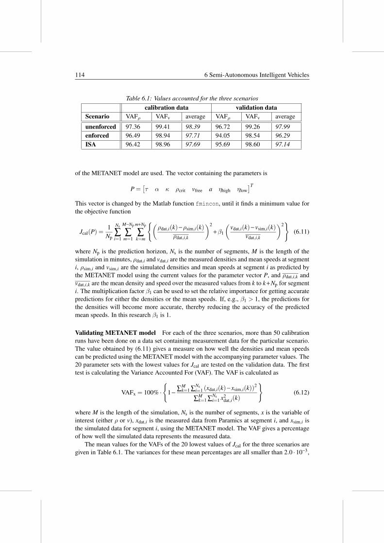
114 6 Semi-Autonomous Intelligent Vehicles
Table 6.1: Values accounted for the three scenarios
calibration data validation data
Scenario VAFρ VAFv average VAFρ VAFv average
unenforced 97.36 99.41 98.39 96.72 99.26 97.99
enforced 96.49 98.94 97.71 94.05 98.54 96.29
ISA 96.42 98.96 97.69 95.69 98.60 97.14
of the METANET model are used. The vector containing the parameters is
P =[
τ α κ ρcrit vfree a ηhigh ηlow
]T
This vector is changed by the Matlab function fmincon, until it finds a minimum value forthe objective function
Jcal(P) =1
Np
Ns
∑i=1
M−Np
∑m=1
m+Np
∑k=m
{
(
ρdat,i(k)−ρsim,i(k)
ρdat,i,k
)2
+β1
(
vdat,i(k)− vsim,i(k)
vdat,i,k
)2}
(6.11)
where Np is the prediction horizon, Ns is the number of segments, M is the length of thesimulation in minutes, ρdat,i and vdat,i are the measured densities and mean speeds at segmenti, ρsim,i and vsim,i are the simulated densities and mean speeds at segment i as predicted bythe METANET model using the current values for the parameter vector P, and ρdat,i,k andvdat,i,k are the mean density and speed over the measured values from k to k +Np for segmenti. The multiplication factor β1 can be used to set the relative importance for getting accuratepredictions for either the densities or the mean speeds. If, e.g., β1 > 1, the predictions forthe densities will become more accurate, thereby reducing the accuracy of the predictedmean speeds. In this research β1 is 1.
Validating METANET model For each of the three scenarios, more than 50 calibrationruns have been done on a data set containing measurement data for the particular scenario.The value obtained by (6.11) gives a measure on how well the densities and mean speedscan be predicted using the METANET model with the accompanying parameter values. The20 parameter sets with the lowest values for Jcal are tested on the validation data. The firsttest is calculating the Variance Accounted For (VAF). The VAF is calculated as
VAFx = 100% ·
{
1 −∑M
k=1 ∑Nsi=1 (xdat,i(k)− xsim,i(k))
2
∑Mk=1 ∑
Nsi=1 x2
dat,i(k)
}
(6.12)
where M is the length of the simulation, Ns is the number of segments, x is the variable ofinterest (either ρ or v), xdat,i is the measured data from Paramics at segment i, and xsim,i isthe simulated data for segment i, using the METANET model. The VAF gives a percentageof how well the simulated data represents the measured data.
The mean values for the VAFs of the 20 lowest values of Jcal for the three scenarios aregiven in Table 6.1. The variances for these mean percentages are all smaller than 2.0 ·10−3,

6.6 Case study 115
Table 6.2: Parameter values for the METANET model
Scenario τ α κ ρcrit vfree a ηhigh ηlow
unenforced 0.0042 -0.0521 126.91 26.69 176.78 1.62 204.60 153.59enforced 0.0025 -0.2737 176.69 29.28 169.10 1.37 167.35 91.96ISA 0.0061 -0.1257 137.05 29.39 169.21 2.65 233.81 128.31
5 10 15
5
10
15
ρdat
(veh/km)
Se
gm
en
t
0
10
20
30
40
50
5 10 15
5
10
15
ρsim
(veh/km)
0
10
20
30
40
50
5 10 15
5
10
15
ρdat
−ρsim
(veh/km)
−20
−10
0
10
20
5 10 15
5
10
15
Time (s)
vdat
(km/h)
Se
gm
en
t
0
50
100
150
5 10 15
5
10
15
vsim
(km/h)
Time (s)
0
50
100
150
5 10 15
5
10
15
Time (s)
vdat
−vsim
(km/h)
−20
−10
0
10
20
Figure 6.9: Illustration of validation
so the 20 best parameter sets give quite similar results. From the table it can be seen thatthe values for the validation data are lower compared to the values for the calibration data.This is as expected, since the parameters are optimised to represent the calibration data.Another observation from the table is that the densities are predicted less accurate than themean speeds. The prediction of the densities can be improved by taking a smaller valuefor the weighting factor β1 in (6.11). This is not done due to limited time, but it willprobably improve the overall performance of the controller, since it will give more accuratepredictions. Despite the lower accuracy of the densities, the average VAFs for both thecalibration data and the validation data are good. Per scenario, the parameter set resulting inthe highest average VAF is used for the controller prediction model. The parameter valuesused are shown in Table 6.2.
Besides validating the obtained parameters by calculation, we also provide an illustra-tion of this validation. In order to do so, some 15 minute predictions are done, and plottedin a figure, together with the measured data, and the difference of both. An example ofsuch a plot is given in Figure 6.9. The figure shows the prediction from the 80th to the 95thminute, for the unenforced speed limit scenario. ρdat and vdat are the measured densities andmean speeds from Paramics, ρsim and vsim are the simulated densities and mean speeds aspredicted using the METANET model. At this time, a shock wave is starting to enter thenetwork, and no control is used. The shock wave is clearly visible, starting at the upper leftcorner. This visualisation shows that the speed at which the shock wave moves upstreamis quite accurate, and also the width is predicted well. The prediction is much smootherthan the measured situation, but it needs not give more detail for use in the controller. For

116 6 Semi-Autonomous Intelligent Vehicles
both the calibration and validation, the measured data is used to get the future states at theboundary segments.
6.6.4 Control problem
When no control is applied to the network, and the traffic demand stays high, the traffic jamwill continue to move upstream, thereby slowing down all vehicles passing it. The aim ofthe traffic controller is to reduce or dissolve this traffic jam, and thereby reducing the timevehicles spend in the monitored part of the traffic network. The corresponding performancefunction Jperf(k) used in the calculation of the total time spent as in (6.3.2), is then given by
Jperf(k) = TctrlN(0)K + T 2ctrl
K
∑k=0
(K − k)(qdem − qout(k)) [veh ·h] (6.13)
where Tctrl is the controller time step ( 160
hour), N(0) is the number of vehicles on thesegments 1 to 20 at k = 0 3, K is the number of time steps taken into account, qdem is theconstant demand used for the simulation (desired inflow), and qout is the outflow measuredat the 20th segment. In the total MPC objective function given in (6.3.2), we have alsoincluded a penalty term with λ1 = 10 and λ2 = 10.
In order to be able to compare the different situations for all scenarios at different trafficdemands, the mean travel time per vehicle is calculated. This is done using
TPV(K) = 60 ·TTS(K)
TctrlKqdem
[min] (6.14)
where TTS(K) is the TTS calculated using (6.3.2). The factor 60 is used to convert hoursinto minutes. The time per vehicle gives the average time it took a vehicle to pass the 10kilometres long highway. In order to compare the different situations and demands, thetimes per vehicle are normalised based on an ideal situation, where the mean speed is 120km/h in every segment at every time instant. In this case the TPV for the 10 kilometre longhighway part is
TPVnorm = 60 ·10
120= 5 [min] (6.15)
As a constraint, the dynamic speed limits are given a maximum and minimum allowedvalue. The upper bound for the speed limits is 120 km/h, and the lower bound value is 40km/h. For the calculation of the optimal control values, all speed limits are constrained tothis range. When the optimal values are found, they are rounded to a multiplicity of 10km/h, since this is more clear for human drivers, and also technically feasible without largeinvestments.
6.6.5 Results and analysis
When the density is high, it is more difficult to control the traffic, since the mean speedmight already be below the control speed (see the definition of vdes in (6.1)). Therefore,simulations are done using densities at which the shock wave can dissolve without using
3For the calculation of the TTS, the first 10 minutes of the measured data are rejected. Since the simulationstarts with no vehicles in the network, we take this time to initialise.

6.6 Case study 117
Table 6.3: Measured results for the unenforced speed limit scenario
qdem Case #1 #2 #3 #4 #5 TTS: mean (std) TPV
4700 no shock wave 494.73 452.15 435.98 414.88 428.30 445.21 (6.9%) 5:41
4700 uncontrolled 520.42 517.48 536.13 475.98 539.58 517.92 (4.9%) 6:36
4700 controlled 513.45 488.43 521.35 479.75 500.75 (4.0%) 6:24
4900 no shock wave 493.90 472.60 492.78 521.10 489.43 493.96 (3.5%) 6:03
4900 uncontrolled 635.10 584.92 643.72 571.85 588.63 604.84 (5.3%) 7:24
4900 controlled 575.30 654.12 589.77 572.15 597.84 (6.4%) 7:19
control, and at densities where the shock wave remains. For each scenario, five simulationsfor three different cases are done, each with a duration of one hour. The results of thesimulations are reported in Tables 6.3, 6.4, and 6.5. Each table contains the traffic demandqdem, the case as discussed in Section 6.6, the total time spent calculated using (6.13) forthe five simulations, the mean value and standard deviation (as a percentage of the meanvalue) of the total time spent, and the resulting travel time per vehicle calculated using(6.14). The standard deviation gives a measure of the accuracy of the mean value. Forlower percentages, the obtained mean value for the TTS is more accurate.
Unenforced speed limits
When the speed limits are unenforced, the desired free-flow speed is assumed to be about10% higher than the speed limit. The desired free-flow speed is modelled as a Gaussiandistribution, with a mean value of 110% of the speed limit, and a standard deviation of 8%of the speed limit. Therefore the influence of dynamic speed limits is expected to be high,because the density will be low compared to the other scenarios. For this scenario, shockwaves occur and dissolve at a traffic demand of 4700 veh/h when the on-ramp is used. At atraffic demand of 4900 veh/h, the shock wave remains in the network.
From Table 6.3, it can be concluded that controlling the speed limits in the traffic net-work has a positive effect on the TTS and TPV for the unenforced speed limit scenario.Using the situation without shock waves as a reference, at a demand of 4700 veh/h the TPVis 16.3% higher in the uncontrolled situation, and 12.5% in the controlled situation. Con-sidering the demand of 4900 veh/h, the uncontrolled situation gives an increase of 22.4%in travel time, while the controlled situation gives an increase of 21.0%. Although the im-provements are not very large in this single hour, the long-term improvement is significant.Since the traffic jam is dissolved in the controlled situation, the increase in travel time willbe the average between the controlled hour and the shock-wave-free travel time, resultingin an increased travel time of 10.5% for the high demand situation.
Typical traffic conditions at the traffic demand of 4700 veh/h without control are shownin Figure 6.10. For all four plots in this figure, the vertical axis shows the segment numbers.The traffic flow direction is from the bottom to the top, and since all segments have thesame length, this axis can also be seen as the distance traveled. The upper plot shows thatall speed limits are set to 120 km/h at all times. The second plot from the top shows themean speeds at the segments. The shock wave is shown as the dark area starting at the20th segment after 10 min, moving upstream in time. This shock wave is also shown in the

118 6 Semi-Autonomous Intelligent Vehicles
10 20 40 50 60
5
10
15
S
egm
ent
Speed limits (km/h)
50
100
10 20 40 50 60
5
10
15
20 Speeds (km/h)
Segm
ent
0
50
100
10 20 40 50 60
5
10
15
20 Densities (veh/km)
Segm
ent
0
50
10 20 30 40 50 60
5
10
15
20
Time (min)
Flows (veh/h)
Segm
ent
0
5000
Figure 6.10: Uncontrolled traffic at qdem=4700 veh/h
third plot from the top, which gives the densities. Here the light colour represents the highdensity of the traffic jam. Notice that there are also light, small areas which go downstreamin time. They are the areas of high density, caused by the difference in desired speed for thevehicles. Fast vehicles will meet slower vehicles as they drive on the highway, causing highdensity areas, while creating areas of low density in the upstream direction. These stripesof low and high density are also visible in the fourth plot, which shows the flow. The trafficjam is visible as the dark area of low flow.
When we apply model predictive control to the traffic network, using the same situationas before, the resulting traffic conditions in the network are shown in Figure 6.11. At the 10th
minute, the shock wave enters the part of the highway containing detectors. The controllerresponds by lowering the speed limits at the segments close to the congestion. After 10 min,the traffic jam is almost completely dissolved, as can be seen by the plots.
Enforced speed limits
When the speed limits are enforced, we assume that the desired free-flow speed becomesabout 10% lower than the displayed speed limit. The desired free-flow speed is modelledas a Gaussian distribution, with a mean value of 90% of the speed limit, and a standarddeviation of 8% of the speed limit. Therefore the influence of the dynamic speed limits isexpected to be low, because the density will be high compared to the other scenarios.
For this scenario, shock waves occur and dissolve at a traffic demand of 4500 veh/h. Ata traffic demand of 4700 veh/h, the shock wave remains in the network. Compared to the

6.6 Case study 119
10 20 40 50 60
5
10
15
Speed limits (km/h)
Segm
ent
50
100
10 20 40 50 60
5
10
15
20 Speeds (km/h)
Segm
ent
0
50
100
10 20 40 50 60
5
10
15
20 Densities (veh/km)
Segm
ent
0
50
10 20 30 40 50 60
5
10
15
20
Time (min)
Flows (veh/h)
Segm
ent
0
5000
Figure 6.11: Controlled traffic at qdem=4700 veh/h
Table 6.4: Measured results for the enforced speed limit scenario
qdem Case #1 #2 #3 #4 #5 TTS: mean (std) TPV
4500 no shock wave 589.22 532.23 538.82 624.30 560.45 569.00 (6.7%) 7:35
4500 uncontrolled 580.85 571.20 603.40 627.30 623.12 601.17 (4.1%) 7:55
4500 controlled 615.60 600.32 636.12 575.60 606.91 (4.2%) 8:06
4700 no shock wave 635.52 614.97 583.73 693.12 588.07 623.08 (7.1%) 7:57
4700 uncontrolled 700.33 680.42 659.47 736.15 746.82 704.64 (5.2%) 9:00
4700 controlled 713.20 673.12 686.83 750.40 705.89 (4.8%) 9:01
unenforced speed limit scenario, these demands are lower. This is due to the lower desiredfree-flow speeds, which result in higher densities at the same demand. Therefore the criticaldensity is reached at a lower demand. From Table 6.4, it can be seen that the TTS is largerin the uncontrolled case, due to the traffic jam. The controller is not able to lower the TTSfor both demands, the travel times even slightly increase. At a demand of 4500 veh/h, thetraffic jam increases the travel time by 5.7%. Using traffic control, the travel time increasesby 6.7%, so there is a negative improvement in travel times by using dynamic speed limitcontrol. Due to the small amount of simulations, no solid conclusion can be drawn fromthe mean values for the TTS for both cases, but they are expected to stay almost equal.We conclude that the controller will not improve the TTS, but it will improve traffic safetyby creating a more homogenous traffic flow. The same conclusion can be drawn when thedemand is 4700 veh/h, where the increase in travel time for the uncontrolled situation is

120 6 Semi-Autonomous Intelligent Vehicles
10 20 40 50 60
5
10
15
S
egm
ent
Speed limits (km/h)
50
100
10 20 40 50 60
5
10
15
20 Speeds (km/h)
Segm
ent
0
50
100
10 20 40 50 60
5
10
15
20 Densities (veh/km)
Segm
ent
0
50
10 20 30 40 50 60
5
10
15
20
Time (min)
Flows (veh/h)
Segm
ent
0
5000
Figure 6.12: Uncontrolled traffic at qdem=4700 veh/h
13.1%, and 13.3% for the controlled situation.The homogeneous traffic flow is shown in Figure 6.13. In Figure 6.12 the traffic states
are shown, when the speed limits are uncontrolled, and with a high demand of 4700 veh/hthat results in a remaining traffic jam. When the same demand is used, but dynamic speedlimit control is applied to the network, the traffic jam is dissolved by spreading the vehiclesmore evenly over the highway, as shown in Figure 6.13.
The effect is a more constant speed over the measured area, as shown in the secondplot from above. This increases the safety on the highway. So although the travel timeswill not decrease by applying control, the controller positively affects the traffic situation byimproving the safety.
Intelligent speed adaptation
For the ISA scenario, the desired free-flow speed is about 100% of the speed limit. Thedesired free-flow speed is modelled as a Gaussian distribution, with a mean value of 100% ofthe speed limit, and a standard deviation of 5% of the speed limit. Based on this percentage,the influence of the dynamic speed limits is expected to be good.
When the vehicles are equipped with ISA, shock waves occur and dissolve at a trafficdemand of 4700 veh/h. At a traffic demand of 4900 veh/h, the shock wave remains in thenetwork. The measured TTSs and TPVs for both demands are given in Table 6.5.
From Table 6.5, it is concluded that controlling the speed limits on the traffic network hasa positive effect on the TTS and TPV for the intelligent speed adaptation scenario. Using the

6.6 Case study 121
10 20 40 50 60
5
10
15
Speed limits (km/h)
Se
gm
en
t
50
100
10 20 40 50 60
5
10
15
20 Speeds (km/h)
Se
gm
en
t
0
50
100
10 20 40 50 60
5
10
15
20 Densities (veh/km)
Se
gm
en
t
0
50
10 20 30 40 50 60
5
10
15
20
Time (min)
Flows (veh/h)
Se
gm
en
t
0
5000
Figure 6.13: Controlled traffic at qdem=4700 veh/h
Table 6.5: Measured results for the intelligent speed adaptation scenario
qdem Case #1 #2 #3 #4 #5 TTS: mean (std) TPV
4700 no shock wave 432.38 407.60 461.85 481.47 446.35 445.93 (6.3%) 5:42
4700 uncontrolled 510.70 562.90 506.72 496.40 528.25 520.99 (5.0%) 6:39
4700 controlled 485.90 511.38 491.72 479.35 492.09 (2.8%) 6:17
4900 no shock wave 415.42 473.52 423.43 511.95 513.55 467.57 (9.9%) 5:44
4900 uncontrolled 596.58 619.15 540.70 629.22 658.70 608.87 (7.3%) 7:27
4900 controlled 468.77 475.83 535.53 492.45 493.15 (6.1%) 6:02

122 6 Semi-Autonomous Intelligent Vehicles
10 20 40 50 60
5
10
15
Se
gm
en
t
Speed limits (km/h)
50
100
10 20 40 50 60
5
10
15
20 Speeds (km/h)
Se
gm
en
t
0
50
100
10 20 40 50 60
5
10
15
20 Densities (veh/km)
Se
gm
en
t
0
50
10 20 30 40 50 60
5
10
15
20
Time (min)
Flows (veh/h)
Se
gm
en
t
0
5000
Figure 6.14: Uncontrolled traffic at qdem=4900 veh/h
case without shock waves as a reference, at a demand of 4700 veh/h the travel time is 16.8%longer in the uncontrolled situation, and 10.4% in the controlled situation. Considering thedemand of 4900 veh/h, the uncontrolled situation gives an increase of 30.2% in travel time,while the controlled situation gives an increase of 5.5%.
Typical traffic conditions at the traffic demand of 4900 [veh/h] without traffic controlare shown in Figure 6.14. The figure shows the remaining shock wave, which enters thenetwork at the 10th minute, and remains in the network with a constant length. Withoutcontrol, the traffic jam will continue to move upstream in the traffic network.
When control is applied to the traffic network using the same traffic demand, the trafficjam is dissolved, as shown in Figure 6.15. The traffic situation is improved in the part ofthe network where the measurements are done, and also the upstream part of the networkwill not suffer from higher travel times due to a traffic jam. Controlling a small part of thenetwork thus has a positive effect for a larger part of the network.
6.7 Summary
In this chapter, we have investigated the possibility of using semi-autonomous IVs (espe-cially IVs equipped with ISA systems) to improve the performance of the traffic system.We have discussed how model predictive control (MPC) approach can be used to determ-ine optimal, dynamic speeds limits for the semi-autonomous traffic systems. We have alsopresented the details of the plugins that allow the simulation software Paramics to simulatethe behaviour of semi-autonomous vehicles. This intermediate approach has been illustratedusing a case study based on simulations. The improvement on the network performance ob-tained by deploying ISA systems has been compared with other scenarios, like unenforcedand enforced speed limits.

6.7 Summary 123
10 20 40 50 60
5
10
15
Speed limits (km/h)
Se
gm
en
t
50
100
10 20 40 50 60
5
10
15
20 Speeds (km/h)
Se
gm
en
t
0
50
100
10 20 40 50 60
5
10
15
20 Densities (veh/km)
Se
gm
en
t
0
50
10 20 30 40 50 60
5
10
15
20
Time (min)
Flows (veh/h)
Se
gm
en
t
0
5000
Figure 6.15: Controlled traffic at qdem=4900 veh/h

124 6 Semi-Autonomous Intelligent Vehicles

Chapter 7
Conclusions and
Recommendations
This chapter mainly summarises our work in this thesis. Section 7.1 highlights the maincontributions of this thesis to the state-of-the-art. In Section 7.2, the main conclusionsdrawn at the end of each chapter are summarised. Finally, in Section 7.3, open problemsand recommendations for future research are discussed.
7.1 Main contributions
The approach we have considered in this thesis for advanced traffic system is based on theIVHS traffic system. An IVHS consist of interacting roadside infrastructures and vehiclesequipped with advanced in-vehicle technologies (IVs). The fully automated IVs are organ-ised in platoons with short intraplatoon distances, and larger distances between platoons.The proposed approach aims at enabling and sustaining an efficient operation of the IVHSsystem through the used of advanced control methods and for this purpose, it utilises tech-nological advancements from both the automotive and the traffic management fields. Ourmain contributions to the state-of-the-art in IVHS-based traffic control and managementapproaches are:
• The proposal of a new hierarchical, distributed framework to control large-scaleIVHS-based traffic networks,
• The development of control algorithms that can be deployed at different (roadside andarea) levels of IVHS-based traffic management systems.
The first contribution of this thesis was the proposal of a new framework to control andmanage large-scale IVHS-based traffic systems in a well-structured and distributed manner.In the proposed framework, the traffic control and coordination tasks are distributed amongseveral levels in the hierarchy and also among various controllers at the same level.
Secondly, the focus was on the development of control methodologies that can be im-plemented within the context of our framework. Most of the existing IVHS frameworksprimarily focus on vehicle level controlling problems. In particular, they mainly deal with
125

126 7 Conclusions and Recommendations
the control issues that result due to the actual implementation of platooning approaches andIV technologies in vehicles. However, the control problems at tactical and navigationallevels did not yet receive much attention and thus motivated us to work on these lines ofresearch. More specifically, in this thesis, we have designed control methodologies for theroadside and area controllers to improve the performance of large-scale IVHS-based trafficsystems.
In particular, we have developed an MPC-based control algorithm that the roadside con-troller can use to combine ramp metering (or other conventional roadside-based traffic con-trol measures) with intelligent speed adaptation (ISA), lane allocation measures, and other(future) IV-based control measures, and to determine system-optimum control signals forthese control measures. In our framework, the navigational control tasks (route guidance)are handled by the area controller. Thus we have also developed and implemented an op-timal control algorithm for the area controller to optimally route the platoons on the set ofinterconnected highways. To solve the routing problem, our control algorithm either usedmixed-integer linear or real-valued nonlinear programming techniques.
For the other higher levels in the control hierarchy, similar control approaches, alsobased on MPC but with even more aggregate models can be used.
7.2 Conclusions
7.2.1 Main conclusions
The main conclusions of this thesis are:
• A multi-level framework is necessary for the traffic management and control pur-poses. This multi-level structure should range from a vehicle controller at the bottomlevel to the traffic management controllers at roadside, area, and regional at higherlevels.
• MPC approach is a good method for traffic management and control purposes in bothroadside and area controllers.
• The potential improvement in the traffic flow obtained from the multi-level frameworkhas been illustrated using case studies. By the combination of IV-based platoonsand multi-level framework, performance improvement of 10–30 % is possible. Theaccuracy of the performance improvement depends on the considered traffic demand,scenario, and set-up, and on more experiments.
7.2.2 Conclusions per chapter
In this section, we summarise the conclusions drawn from each chapter in this thesis.In Chapter 2, we have presented a detailed review of some of the most frequently used
control methodologies. These methods are used for controlling a human driven highwaytraffic system. We have also illustrated the working procedure of these control techniquesusing a common application such as ramp metering. Having discussed the state-of-the-art ofcurrently applied control methods, we then focused on control architectures for IVHS. Thisincluded the discussion of various existing architectures such as PATH, Dolphin, Auto21

7.2 Conclusions 127
CDS, CVIS, SafeSpot, and PReVENT. Based on our literature survey, we have made acomparative analysis of the control methods and the control architectures to assess theirsimilarities and their differences. The conclusions from this analysis clearly indicated theadvantages offered by using a hierarchical structuring and also showed the importance ofand need for a flexible and traffic-adaptive control design methodology. The other topicdiscussed in this chapter is IVs and their functionalities, which on the long-term includeplatooning. The platooning approach, which allows vehicles to maintain small intra-platoondistances and to travel with high speeds, along with the necessary driver assistance systemssuch as cooperative ACC (for maintaining safe distance), ISA, and dynamic route guidancesystems will offer considerable benefits to traffic flow improvement. However, the roadsideinfrastructure is currently unaware of these potential benefits. This leads us to question whyroadside traffic control measures are not (yet) adapted to include this intelligence.
Based on the knowledge gained from our survey and analysis, we have introduced anew framework for IVHS that integrates the intelligence in roadside infrastructure and inplatoons of automated IVs. A detailed description of our new framework is given in Chapter3. Our framework also allows vehicle-vehicle and vehicle-roadside communications similarto the other existing IVHS architectures. However, our framework differs mainly in terms ofcombining the existing conventional traffic control measures and the IV technologies, andviewing them as IV-based control measures.
Chapter 4 mainly dealt with the problem formulation and the control-related issues ofroadside controllers. From our preliminary study on control methods, we have decided toimplement an MPC approach to perform the IV-based roadside traffic control operations.More specifically, the MPC algorithm discussed in this chapter determines optimal ISAspeed limits and lane allocations as well as optimal release times for the platoons at the on-ramps. Since MPC is an on-line, model-based approach with a receding horizon mechanism,we have presented some traffic models that could be used for simulation and prediction atthe roadside level, and have discussed the control issues related to optimisation methods,and to the choice of controller settings such as the prediction and control horizons andthe number of control signals. The simulations based on the MPC approach reported inChapter 4, compare the performance of the IVHS traffic system to the performance of ahuman-driven traffic system. For the defined case study, the platoon-based approach resultsin a better performance compared to the situation with controlled human drivers. However,our approach poses some challenges on computational complexity. Determining optimalcontrol signals that consist of both real and integer valued variables such as ISA speeds andlane allocation for each platoon, consumes more time and requires more system memory toperform the computations.
In Chapter 5, we have focused on area controllers, which control a set of interconnectedhighways and coordinate the activities of various roadside controllers in their area. In par-ticular, this controller assigned optimal routes to the platoons in the IVHS. As mentionedearlier, determining control measures for each platoon proves to be computationally de-manding, and hence motivated us to propose two simplified but fast simulation models todescribe the flows of platoons in the network. For the first model, which only considersflows and queues lengths, we have shown that the optimal route choice control problemcan be approximated by a linear or a mixed-integer linear problem. With a simple casestudy we have illustrated that this results in a balanced trade-off between optimality andcomputational efficiency. The second model is a macroscopic model based on an existing

128 7 Conclusions and Recommendations
traffic flow model for human drivers (METANET), which we have adapted to fit the pla-toon framework. For this model, the optimal route choice control problem results in anoptimisation problem with only real-valued optimisation variables. This approach was alsoillustrated with a simple case study involving a comparison between human drivers and anIVHS with platoons of IVs. As expected, the deployment of IVs in the system resulted in abetter performance than the human driven traffic system.
Chapter 6 mainly showed the possibility of equipping vehicles with advanced in-carsystems in an existing simulation software and also investigated the improvement that couldbe attained by implementing ISA at the vehicle level. We have used the traffic simulationsoftware PARAMICS to represent the current traffic system and we have developed plug-ins for the partially automated vehicles to capture their reaction to the control measures.We have implemented the roadside controller in Matlab and since there was no existinginterface between the two software programs, we have also created a plug-in to simulatethe behaviour of IV-based vehicles. We have investigated the effect of control on the trafficsystem driven by human drivers and on the system driven with partially automated vehiclesusing a simple case study. The system with partially automated vehicles offered betterperformance improvement than the current conventional traffic system.
7.3 Open problems and recommendations for future re-
search
Every research work has a room for improvement. In this section, we discuss some propos-als for future research in the field of traffic management and control with intelligent vehiclesin various directions:
• Model considerations,
• Controller considerations,
• Complexity and implementation issues,
• Alternative approaches,
• Transition aspects.
Model considerations
• Since MPC is a model-based approach, we are in need of fast and simple modelsfor prediction purposes. In this thesis except in Chapter 7, to filter out the effects ofmodel mismatch errors, we have deployed the same simulation model for predictionpurposes. The effect of such errors should be investigated by considering set-ups inwhich the simulation and the prediction model are different.
• Especially for the roadside controller described in Chapter 4, the currently used pre-diction model is still too time-consuming. Hence, we should also develop faster andsimpler models for the traffic flows on individual freeway stretches, while still guar-anteeing a sufficiently high degree of accuracy. However, e.g., for complex junctions,
7.3 Open problems and recommendations for future research 129
we might still require a detailed representation of the traffic system. Therefore, weshould develop so called multi-resolution prediction models with different degrees ofaccuracy in certain regions of interest.
• Each layer in our IVHS framework uses a different level of details of the traffic sys-tem, and also deals with different sets of inputs and control outputs. In particular,the roadside controller can use Paramics, or the big-car model, and the area control-ler can work with flow-based models. Therefore, we should develop interfaces tobring consistency among the inputs and outputs obtained from different layers of theframework.
• We should design and develop new, fast models with required accuracy for all levels.
Controller considerations
• In this thesis, the roadside controller has performed the coordination and integrationof different control measures. In Chapter 4, we have in particular combined ISA andoptimal lane allocations (IV-based control measure) along with the ramp metering(roadside control measure). However, we can extend this combination to include othertraffic IV-based control measures that might be developed by both the transportationand vehicle industry in the near future. Also, the computational complexity of thecontrol problem can be analysed using analytical methods or empirical methods.
• Currently, the roadside controller had no control over the platoon sizes and the platoonsize was assumed to be a constant value in all our case studies. If this control measureis also taken into account, then the roadside controller can have more control over thetraffic scenario. Platoons can then vary from a single car to a very large number.
• Depending on the nature of the traffic problem, the controller can use continuousoptimisation (for ISA and ramp metering), integer optimisation (for optimal lane al-locations) or a combination of both techniques to find an optimal solution. Findingan optimal solution for an integer-valued problem poses more computational prob-lems than real-valued problems. Since the determination of optimal platoon sizesalso falls under the integer optimisation problems, the roadside controller should beable to consider these issues and to deal with the computational complexities (seenext subsection).
• If we extend the scope of our approach to urban or mixed urban-freeway networks,then the controller should combine control measures from both traffic systems andshould be able to handle the computational issues discussed above.
• In our framework, we allowed interactions only among different levels and not at thesame level. For instance, the roadside controllers do not interact among themselvesto coordinate some of their activities. For our future research, we should compareand investigate the potential benefits that could be achieved using decentralised anddistributed coordination at the same level.
• Higher-level controllers such as regional and supraregional controllers will provideroute guidance instructions to a collection of area controllers. This would then require

130 7 Conclusions and Recommendations
us to design control methods based on aggregated, simple flow models that wouldrepresent the traffic flows on different areas under consideration.
• Different objective functions or a combination of objective functions should be con-sidered to analyse the performance of the traffic system. Some examples of possiblecost functions are energy saving, fuel emissions, throughput, safety, etc. To solve theresulting multi-objective problems, we could use multi-objective optimisation meth-ods such as evolutionary algorithms, weighted-sum single aggregate objective func-tions, goal attainment etc.
Complexity and implementation issues
• The computational complexity of the proposed approach is still an issue and needs tobe analysed, in particular for the roadside controller. Hence, we should investigateways to increase the efficiency of the current approach or develop alternative controlmethods. Some suggestions for the current MPC approach can then be to use block-ing techniques (same solution applied for a certain number of consecutive time steps),to start the optimisation with a good initial solution obtained through approximations,to use a multi-level approach to deal with the mixed integer optimisation problems, toreduce the control horizons, to increase the number of vehicles in a platoon, etc. Thecomplexity of the control approach (i.e., execution time and memory requirements)mainly depends on the number of control variables and on the type of control vari-ables (integer, real-valued). We should analyse this complexity either analytical orempirical ways.
• Extensive evaluation and assessment of the framework through a wide range of casestudies and scenarios at different levels and with the entire framework should be per-formed. These set-ups could also use a detailed IV-based vehicle models for trafficsimulations.
• Another topic will the real-time application issues. Due to the optimisation over bothreal and integer variables, the controller implemented in Chapter 4 is unable to func-tion in real time. Since multi-start optimisation has been used, an improvement in thisdirection could be attained by implementing the controller in such a way that it cantake the advantage of the upcoming trends in multi-processor systems and distributedoptimisation.
Alternative approaches
• In this research, our framework was analysed mainly using the MPC approach. Later,we should also analyse the performance of the framework using other control ap-proaches. For instance, we could use alternative control approaches such as fuzzylogic, artificial neural networks, gain scheduling, or LPV methods.
• On the other hand, one could consider a swarm-like autonomous driving system –a completely different approach to our hierarchical framework. More specifically,this approach does not allow/consider roadside-based controllers. In this approach,the vehicles try to aggregate themselves in groups, make their decisions based only

7.3 Open problems and recommendations for future research 131
on local information. For this approach, one will have to develop control strategiesfor the movement of individual vehicles inside a swarm by means of cooperation,coordination or negotiation with their neighbours.
Transition aspects
• In this research, vehicles in the traffic system were assumed to be completely auto-mated and homogeneous (only IVs). An interesting research topic is to allow a trafficsystem with heterogeneous intelligent vehicles (cars, trucks, etc.) and also with dif-ferent penetration rates of IVs, i.e., situations of mixed traffic with both human driversand platoons of automated IVs, if tractable at all.
• In an urban-freeway traffic system, the roadside controller should be able to handle thetransition situation from human-driven vehicles in urban networks to autonomouslydriven platoons on freeways, and vice versa. As a suggestion to support this transition,we could allow the roadside controller to use traffic signals as a control measure sothat the vehicles do not have to wait too long at the on-ramp, by which one can preventthe on-ramp queue from spilling back to the urban network.
• Legal, social, economic and other issues involved in the transition of the conventionaltraffic system to the proposed IVHS system also need to be addressed. These issuescan be stated in terms of social acceptance of the system, investments required forimplementations, etc.

132 7 Conclusions and Recommendations

Bibliography
[1] A. Aamodt and E. Plaza. Case-based reasoning: Foundational issues, methodologicalvariations, and system approaches. AI Communications, 7(1):39–59, March 1994.
[2] AHSRA web site. http://www.ahsra.or.jp/. Last visited on November 4, 2008.
[3] K. J. Åström and B. Wittenmark. Computer-Controlled Systems — Theory and Ap-
plications. Prentice-Hall, Upper Saddle River, New Jersey, 3rd edition, 1997.
[4] K. J. Åstrom, P. Albertos, M. Blanke, A. Isidori, W. Schaufelberger, and R. Sanz,editors. Control of Complex Systems. Springer-Verlag, New York, 2000.
[5] A. Atamtürk and M. W. P. Savelsbergh. Integer-programming software systems. An-
nals of Operations Research, 140(1):67–124, November 2005.
[6] C. Audet and J. E. Dennis Jr. Analysis of generalized pattern searches. SIAM Journal
on Optimization, 13(3):889–903, 2007.
[7] Auto21 CDS web site. http://www.damas.ift.ulaval.ca/projets/auto21/en/index.html.Last visited on December 2, 2008.
[8] S. Bana. Coordinating automated vehicles via communication. Technical ReportUCB-ITS-PRR-2001-20, PATH Research Report, Berkely, California, 2001.
[9] L. D. Baskar, B. De Schutter, and H. Hellendoorn. Decentralized traffic controland management with intelligent vehicles. In Proceedings of the 9th TRAIL Con-
gress 2006 — TRAIL in Motion — CD-ROM, Rotterdam, The Netherlands, November2006.
[10] L. D. Baskar, B. De Schutter, and H. Hellendoorn. Hierarchical traffic control andmanagement with intelligent vehicles. In Proceedings of the 2007 IEEE Intelligent
Vehicles Symposium (IV’07), pages 834–839, Istanbul, Turkey, June 2007.
[11] L. D. Baskar, B. De Schutter, and H. Hellendoorn. Model predictive control forintelligent speed adaptation in intelligent vehicle highway systems. In Proceedings
of the 17th IEEE International Conference on Control Applications, pages 468–473,San Antonio, Texas, September 2008.
133

134 Bibliography
[12] L. D. Baskar, B. De Schutter, and H. Hellendoorn. Intelligent speed adaptation inintelligent vehicle highway systems — A model predictive control approach. In Pro-
ceedings of the 10th TRAIL Congress 2008 — TRAIL in Perspective — CD-ROM,Rotterdam, The Netherlands, October 2008.
[13] L. D. Baskar, B. De Schutter, and J. Hellendoorn. Model-based predictive trafficcontrol for intelligent vehicles: Dynamic speed limits and dynamic lane allocation.In Proceedings of the 2008 IEEE Intelligent Vehicles Symposium (IV’08), pages 174–179, Eindhoven, The Netherlands, June 2008.
[14] L. D. Baskar, B. De Schutter, and J. Hellendoorn. Dynamic speed limits and on-ramp metering for IVHS using model predictive control. In Proceedings of the 11th
International IEEE Conference on Intelligent Transportation Systems (ITSC 2008),pages 821–826, Beijing, China, October 2008.
[15] L. D. Baskar, B. De Schutter, J. Hellendoorn, and A. Tarau. Traffic management forintelligent vehicle highway systems using model-based predictive control. In Pro-
ceedings of the 88th Annual Meeting of the Transportation Research Board, Wash-ington, DC, January 2009. Paper 09-2107.
[16] L.D. Baskar, B. De Schutter, Z. Papp, and J. Hellendoorn. Traffic control and intel-ligent vehicle highway systems: A survey. Technical Report 09-043, Delft Centerfor Systems and Control, Delft University of Technology, Delft, The Netherlands,August 2009. Accepted for publication in IET Intelligent Transport Systems.
[17] T. Bellemans. Traffic Control on Motorways. PhD thesis, Faculty of Applied Sci-ences, K.U.Leuven, Leuven, Belgium, May 2003.
[18] T. Bellemans, B. De Schutter, and B. De Moor. Model predictive control for rampmetering of motorway traffic: A case study. Control Engineering Practice, 14(7):757–767, July 2006.
[19] R. Bellman. Dynamic Programming. Princeton University Press, Princeton, NewJersey, 1957.
[20] A. Bemporad and M. Morari. Control of systems integrating logic, dynamics, andconstraints. Automatica, 35(3):407–427, March 1999.
[21] R. Bishop. A survey of intelligent vehicle applications worldwide. In Proceedings of
the IEEE Intelligent Vehicles Symposium, pages 25–30, Dearborn, Michigan, 2000.
[22] R. Bishop. Intelligent Vehicles Technology and Trends. Artech House, 2005.
[23] R. Bishop. http://www.ivsource.net/, 2005. Last visited on June 2, 2009.
[24] J. Blum and A. Eskandarian. Managing effectiveness and acceptability in intelligentspeed adaptation systems. In International Conference on Intelligent Transportation
Systems, pages 319–324, Toronto, Canada, September 2006.
[25] K. Bogenberger, H. Keller, and A. D. May. A neuro-fuzzy approach for ramp meter-ing. In Proceedings of the 10th International Conference on Road Transport Inform-
ation and Control, pages 101–105, London, England, 2000.

Bibliography 135
[26] A. Bose and P. Ioannou. Mixed manual/semi-automated traffic: a macroscopic ana-lysis. Transportation Research Part C, 11(6):439–462, 2003.
[27] M. Brackstone and M. McDonald. Car-following: A historical review. Transporta-
tion Research Part F, 2(4):181–196, 1999.
[28] M. Broucke and P. Varaiya. The automated highway system: A transportation techno-logy for the 21st century. Control Engineering Practice, 5(11):1583–1590, Novem-ber 1997.
[29] M. Burger. Advanced Traffic Management with Integrated Model Predictive Control.Msc thesis, Delft Center for Systems and Control, Delft University of Technology,Delft, The Netherlands, September 2007.
[30] E. F. Camacho and C. Bordons. Model Predictive Control in the Process Industry.Springer-Verlag, Berlin, Germany, 1995.
[31] E. Camponogara, D. Jia, B. H. Krogh, and S. Talukdar. Distributed model predictivecontrol. IEEE Control Systems Magazine, 22(1):44–52, February 2002.
[32] O. Carsten and F. Tate. Intelligent speed adaptation: The best collision avoidancesystem? In Proceedings of the 17th International Technological Conference on the
Enhanced Safety of Vehicles, pages 1–10, Amsterdam, The Netherlands, 2001.
[33] C. G. Cassandras, D. L. Pepyne, and Y. Wardi. Optimal control of systems with time-driven and event-driven dynamics. In Proceedings of the 37th IEEE Conference on
Decision and Control, pages 7–12, Tampa, Florida, December 1998.
[34] R. Chandler, R. Herman, and E. Montroll. Traffic dynamics studies in car following.Operations Research, 6(2):165–184, June 1958.
[35] H. Chen and F. Allgöwer. Quasi-infinite horizon nonlinear model predictive controlscheme with guaranteed stability. Automatica, 34(10):1205–1217, January 1998.
[36] S. H. Chen, A. J. Jakeman, and J. P. Norton. Artificial intelligence techniques: Anintroduction to their use for modelling environmental systems. Mathematics and
Computers in Simulation, 78(2):379–400, July 2008.
[37] S. Cheon. An overview of automated highway systems and the social institutionalchallenges they face. Technical Report UCTC No. 624, University of California,Berkeley, California, 2002.
[38] D. W. Clarke, C. Mohtadi, and P. S. Tuffs. Generalized predictive control – Part I.The basic algorithm. Automatica, 23(2):137–148, March 1987.
[39] L. S. Comte. New systems: new behaviour? Transportation Research Part F, 3(2):95–111, May 2000.
[40] C. Cordier, H. Marchand, R. Laundy, and L. A. Wolsey. bc-opt: A branch-and-cutcode for mixed integer programs. Mathematical Programming, Series A, 86(2):335–353, 1999.

136 Bibliography
[41] J. Cuena, J. Hernández, and M. Molina. Knowledge-based models for adaptive trafficmanagement systems. Transportation Research Part C, 3(5):311–337, October 1995.
[42] CVIS web site. http://www.cvisproject.org/. Last visited on November 4, 2008.
[43] C. F. Daganzo. Fundamentals of Transportation and Traffic Operations. PergamonPress, 1997.
[44] C. F. Daganzo. A continnum theory of traffic dynamics for freeways with speciallanes. Transportation Research Part B, 31(2):83–102, 1997.
[45] S. Darbha and K. R. Rajagopal. Intelligent cruise control systems and traffic flowstability. Transportation Research Part C, 7(6):329–352, December 1999.
[46] L. Davis. Handbook of Genetic Algorithms. Van Nostrand Reinhold, New York,1991.
[47] L. C. Davis. Effect of adaptive cruise control systems on traffic flow. Physical Review
E, 69:1–8, 2004.
[48] B. De Schutter, S. P. Hoogendoorn, H. Schuurman, and S. Stramigioli. A multi-agent case-based traffic control scenario evaluation system. In Proceedings of the
IEEE 6th International Conference on Intelligent Transportation Systems (ITSC’03),pages 678–683, Shanghai, China, October 2003.
[49] R. W. Eglese. Simulated annealing: A tool for operations research. European Journal
of Operational Research, 46(3):271–281, June 1990.
[50] R. E. Fenton. IVHS/AHS: Driving into the future. IEEE Control Systems Magazine,14(6):13–20, December 1994.
[51] R. Fletcher and S. Leyffer. Numerical experience with lower bounds for MIQPbranch-and-bound. SIAM Journal on Optimization, 8(2):604–616, May 1998.
[52] A. V. Fursikov. Optimal Control of Distributed Systems: Theory and Applications.American Mathematical Society, Boston, Massachusetts, 2000.
[53] M. R. Garey and D. S. Johnson. Computers and Intractability: A Guide to the Theory
of NP-Completeness. W. H. Freeman and Company, San Francisco, California, 1979.
[54] V. Gazi and K. M. Passino. Stability of a one-dimensional discrete-time asynchron-ous swarm. IEEE Transactions on Systems, Man and Cybernetics, Part B: Cybernet-
ics, 35(4):834–841, August 2005.
[55] D. Gazis, R. Herman, and R. Rothery. Nonlinear follow the leader models of trafficflow. Operations Research, 9(4):545–567, June 1961.
[56] M. Gelfand and S. V. Fomin. Calculus of Variations. Dover Publications, New York,1991.

Bibliography 137
[57] D. N. Godbole, J. Lygeros, E. Singh, A. Deshpande, and A. E. Lindsey. Design andverification of communication protocols for degraded modes of operation of AHS. InProceedings of the 34th IEEE Conference on Decision and Control, pages 427–432,New Orleans, Louisiana, 1995.
[58] F. L. Hall and K. Agyemang-Duah. Freeway capacity drop and the definition ofcapacity. Transportation Research Record, (1320):91–98, 1991.
[59] R. Hall and C. Chin. Vehicle sorting for platoon formation: Impacts on highwayentry and throughput. Transportation Research Part C, 13(5):405–420, 2005.
[60] S. Hallé, B. Chaib-draa, and J. Laumonier. Car platoons simulated as a multiagentsystem. In Proceedings of the 4th Workshop on Agent-Based Simulation, pages 57–63, Montpellier, France, 2003.
[61] D. Hammerstrom. Working with neural networks. IEEE Spectrum, 30(7):46–53, July1993.
[62] F. Hayes-Roth. Rule-based systems. Communications of the ACM, 28(9):921–932,1985.
[63] J. K. Hedrick, M. Tomizuka, and P. Varaiya. Control issues in automated highwaysystems. IEEE Control Systems Magazine, 14(6):21–32, December 1994.
[64] A. Hegyi. Model Predictive Control for Integrating Traffic Control Measures. PhDthesis, Delft University of Technology, Delft, The Netherlands, February 2004.TRAIL Thesis Series T2004/2.
[65] A. Hegyi, B. De Schutter, S. P. Hoogendoorn, R. Babuška, and H. van Zuylen. Fuzzydecision support system for traffic control centers. In Proceedings of the European
Symposium on Intelligent Techniques (ESIT 2000), pages 389–395, Aachen, Ger-many, September 2000. Paper BC-01-2.
[66] A. Hegyi, B. De Schutter, and J. Hellendoorn. Optimal coordination of variable speedlimits to suppress shock waves. IEEE Transactions on Intelligent Transportation
Systems, 6(1):102–112, March 2005.
[67] A. Hegyi, B. De Schutter, and J. Hellendoorn. Model predictive control for optimalcoordination of ramp metering and variable speed limits. Transportation Research
Part C, 13(3):185–209, June 2005.
[68] D. Helbing. Gas-kinetic derivation of navier-stokes-like traffic equations. Physical
Review E, 53(3):2266–2381, 1996.
[69] M. R. Hestenes. Calculus of Variations and Optimal Control Theory. John Wileyand Sons, New York, 1966.
[70] M. Hjälmdahl, S. Almqvist, and A. Várhelyi. Speed regulation by in-car active accel-erator pedal - effects on speed and speed distribution. IATSS Research, 26(2):60–66,May 2002.

138 Bibliography
[71] R. Holve, P. Protzel, and K. Naab. Generating fuzzy rules for the acceleration controlof an adaptive cruise control system. In Proceedings of the 1996 Biennial Confer-
ence of the North American Fuzzy Information Processing Society, pages 451–455,Berkeley, California, 1996.
[72] S. P. Hoogendoorn and P. H. L. Bovy. Multiclass macroscopic traffic flow modelling:A multilane generalisation using gas kinetic theory. In Proceedings of the 14th Inter-
national Symposium of Transportation and Traffic Theory, pages 27–50, Adelaide,Australia, 1999. Elsevier Science Ltd.
[73] S. P. Hoogendoorn, B. De Schutter, and H. Schuurman. Decision support in dynamictraffic management. Real-time scenario evaluation. European Journal of Transport
and Infrastructure Research, 3(1):21–38, 2003.
[74] R. Horowitz and P. Varaiya. Control design of an automated highway system. Pro-
ceedings of the IEEE: Special Issue on Hybrid Systems, 88(7):913–925, July 2000.
[75] A. Hsu, F. Eskafi, S. Sachs, and P. Varaiya. Design of platoon maneuver protocols forIVHS. Technical Report 96-21, University of California, Berkeley, California, 1991.
[76] A. Hsu, F. Eskafi, S. Sachs, and P. Variaya. Protocol design for an automated highwaysystem. Discrete Event Dynamic Systems: Theory and Applications, 2(1):183–206,1993.
[77] P. Ioannou and C. C. Chien. Autonomous intelligent cruise control. IEEE Transac-
tions on Vehicular Technology, 42(4):657–672, November 1993.
[78] N. R. Jennings. A roadmap of agent research and development. Autonomous Agents
and Multi-Agent Systems, 1(1):7–38, July 1998.
[79] D. R. Jones. DIRECT global optimization algorithm. In Encyclopedia of Op-
timization, volume 1, no. 1, pages 431–440. Kluwer Academic Publishers, Bo-ston,Massachusetts, 2001.
[80] R. K. Jurgen. Smart cars and highways go global. IEEE Spectrum, 28(5):26–36, May1991.
[81] P. Kachroo and K. Özbay. Feedback Control Theory for Dynamic Traffic Assignment.Advances in Industrial Control. Springer-Verlag, Berlin, 1999.
[82] A. Karimi and A. Gupta. Incident management system for Santa Monica Smart Cor-ridor. In Proceedings of the 63rd Annual Meeting of the Institute of Transportation
Engineers, pages 180–185, The Hague, The Netherlands, 1993.
[83] A. Kesting, M. Treiber, M. Schönhof, F. Kranke, and D. Helbing. Jam-avoiding ad-aptive cruise control ACC and its impact on traffic dynamics. In Traffic and Granular
Flow, pages 633–643. Berlin, Germany: Springer-Verlag, 2005.
[84] S. Kim, M. E. Lewis, and C. C. White III. Optimal vehicle routing with real-timetraffic information. IEEE Transactions on Intelligent Transportation Systems, 6(2):178–188, June 2005.

Bibliography 139
[85] D. E. Kirk. Optimal Control Theory: An Introduction. Prentice-Hall, EnglewoodCliffs, New Jersey, 1970.
[86] G. J. Klir and B. Yuan. Fuzzy Sets and Fuzzy Logic: Theory and Applications.Prentice-Hall, Upper Saddle River, New Jersey, 1995.
[87] E. Kometani and T. Sasaki. Dynamic behaviour of traffic with a nonlinear spacingspeed relationship. In Proceedings of the Symposium for Theory Traffic Flow, pages105–109, Research Laboratories, General Motors, New York, 1959.
[88] A. Kotsialos and M. Papageorgiou. Freeway ramp metering: An overview. In Pro-
ceedings of the 3rd Annual IEEE Conference on Intelligent Transportation Systems
(ITSC 2000), pages 228–239, Dearborn, Michigan, October 2000.
[89] A. Kotsialos and M. Papageorgiou. Efficiency and equity properties of freewaynetwork-wide ramp metering with AMOC. Transportation Research Part C, 12(6):401–420, 2004.
[90] A. Kotsialos, M. Papageorgiou, and A. Messmer. Optimal coordinated and integ-rated motorway network traffic control. In Proceedings of the 14th International
Symposium of Transportation and Traffic Theory (ISTTT), pages 621–644, Jerusalem,Israel, July 1999.
[91] A. Kotsialos, M. Papageorgiou, C. Diakaki, Y. Pavlis, and F. Middelham. Trafficflow modeling of large-scale motorway networks using the macroscopic modelingtool METANET. IEEE Transactions on Intelligent Transportation Systems, 3(4):282–292, December 2002.
[92] A. Kotsialos, M. Papageorgiou, M. Mangeas, and H. Haj-Salem. Coordinated andintegrated control of motorway networks via non-linear optimal control. Transport-
ation Research Part C, 10(1):65–84, 2002.
[93] A. Kotsialos, M. Papageorgiou, M. Mangeas, and H. Haj-Salem. Coordinated andintegrated control of motorway networks via non-linear optimal control. Transport-
ation Research Part C, 10(1):65–84, February 2002.
[94] B. Krause and C. von Altrock. A complete fuzzy logic control approach for existingtraffic control systems. In Mobility for Everyone, Proceedings of the 4th World Con-
gress on Intelligent Transportation Systems, Berlin, Germany, October 1997. Paperno. 2045.
[95] J. A. Laval and C. F. Daganzo. Lane-changing in traffic streams. Transportation
Research Part B, 40(3):251–264, 2006.
[96] N. E. Leonard and E. Fiorelli. Virtual leaders, artificial potentials and coordinatedcontrol of groups. In Proceedings of 40th IEEE Conference on Decision and Control,pages 2968–2973, Orlando, Florida, 2001.
[97] K. Li and P. Ioannou. Modeling of traffic flow of automated vehicles. IEEE Trans-
actions on Intelligent Transportation Systems, 5(2):99–113, June 2004.

140 Bibliography
[98] M. J. Lighthill and G. B. Whitham. On kinematic waves: a theory of traffic flowon long crowded roads. In Proceedings Royal Society, pages 317–345, London,England, August 1955.
[99] J. Linderoth and T. Ralphs. Noncommercial software for mixed-integer linear pro-gramming. Optimization Online, January 2005.
[100] Y. Liu, K. M. Passino, and M. M. Polycarpou. Stability analysis of one-dimensionalasynchronous swarms. IEEE Transactions on Automatic Control, 48(10):1848–1854,October 2003.
[101] J. M. Maciejowski. Predictive Control with Constraints. Prentice-Hall, Harlow,England, 2002.
[102] A. D. May. Traffic Flow Fundamentals. Prentice-Hall, Englewood Cliffs, New Jersey,1990.
[103] M. McDonald, N. B. Hounsell, and S. R. Njoze. Strategies for route guidance systemstaking account of driver response. In Proceedings of the 6th Vehicle Navigation and
Information Systems, pages 328 – 333, Seattle, Washington, July 1995.
[104] A. Messmer and M. Papageorgiou. METANET: A macroscopic simulation programfor motorway networks. Traffic Engineering and Control, 31(9):466–470, 1990.
[105] R. M. Michaels. Perceptual factors in car following. In Proceedings of the 2nd
International Symposium for Theory Road Traffic Flow, pages 44–59, Paris, France,1963.
[106] F. Middelham. Fuzzy logic demo. Technical report, Rijkswaterstaat, AVV, Rotter-dam, The Netherlands, 1993. In Dutch.
[107] K. M. Miettinen. Nonlinear Multiobjective Optimization. Kluwer Academic Pub-lishers, Boston, Massachusetts, 1999.
[108] M. Molina, J. Hernández, and J. Cuena. A structure of problem-solving methodsfor real-time decision support in traffic control. International Journal of Human-
Computer Studies, 49(4):577–600, October 1998.
[109] K. Nagel. Particle hopping models and traffic flow theory. Physical Review E, 53(5):4655–4672, 1996.
[110] H. T. Nguyen and E. A. Walker. A First Course in Fuzzy Logic. Chapman & HallPress, Boca Raton, Florida, 2nd edition, 1999.
[111] M. Nookala and B. Estochen. Minnesota, USA intelligent vehicle initiative. InProceedings of the IEEE Intelligent Vehicles Symposium, pages 533–536, Versailles,France, 2002.
[112] S. A. Nsour, S. L. Cohen, J. E. Clark, and A. J. Santiago. Investigation of the impactsof ramp metering on traffic flow with and without diversion. Transportation Research
Record, (1365):116–124, 1992.

Bibliography 141
[113] U. Palmquist. Intelligent cruise control and roadside information. IEEE Micro, 13(1):20–28, 1993.
[114] M. Papageorgiou. Applications of Automatic Control Concepts to Traffic Flow Mod-
eling and Control. Lecture Notes in Control and Information Sciences. Springer-Verlag, Berlin, Germany, 1983.
[115] M. Papageorgiou, J. M. Blosseville, and H. Hadj-Salem. Modelling and real-timecontrol of traffic flow on the southern part of Boulevard Périphérique in Paris: Part I:Modelling. Transportation Research Part A, 24(5):345–359, September 1990.
[116] M. Papageorgiou, J. M. Blosseville, and H. Haj-Salem. Modelling and real-timecontrol of traffic flow on the southern part of Boulevard Périphérique in Paris: PartII: Coordinated on-ramp metering. Transportation Research Part A, 24(5):361–370,September 1990.
[117] M. Papageorgiou, H. Hadj-Salem, and F. Middelham. ALINEA local ramp meter-ing: Summary of field results. In Proceedings of the 76th Annual Meeting of the
Transportation Research Board, Washington, DC, 1997. Paper no. 970032.
[118] P. M. Pardalos and M. G. C. Resende. Handbook of Applied Optimization. OxfordUniversity Press, Oxford, England, 2002.
[119] L. E. Parker. Designing control laws for cooperative agent teams. In Proceedings
of IEEE International Conference on Robotics and Automation, pages 582–587, At-lanta, Georgia, 1993.
[120] M. Persson, F. Botling, E. Hesslow, and R. Johansson. Stop and go controller foradaptive cruise control. In Proceedings of the IEEE International Conference on
Control Applications, pages 1692–1697, Kohala Coast, Hawaii, 1999.
[121] PReVENT web site. http://www.prevent-ip.org/. Last visited on November 4, 2008.
[122] I. Prigogine and R. Herman. Kinetic Theory of Vehicular Traffic. American Elsevier,New York, 1971.
[123] S. J. Qin and T. A. Badgwell. An overview of industrial model predictive controltechnology. American Institute of Chemical Engineers, 93(316):232–256, June 1997.
[124] B. S. Y. Rao and P. Varaiya. Roadside intelligence for flow control in an IVHS.Transportation Research Part C, 2(1):49–72, 1994.
[125] M. J. Richardson and D. Smith. Design of the driver interface for autonomous intel-ligent cruise control. In Proceedings of the IEE Colloquium on Design of the Driver
Interface, pages 7/1–7/4, London, England, 1995.
[126] S. G. Ritchie. A knowledge-based decision support architecture for advanced trafficmanagement. Transportation Research Part A, 24(1):27–37, January 1990.
[127] S. G. Ritchie and N. A. Prosser. Real-time expert system approach to freeway incid-ent management. Transportation Research Record, (1320):7–16, 1991.
142 Bibliography
[128] D. Roseman and S. S. Tvedten. Santa Monica Freeway Smart Corridor project opera-tional multi-agency traffic management and expert system. In Mobility for Everyone,
Proceedings of the 4th World Congress on Intelligent Transport Systems, Berlin, Ger-many, October 1997. Paper no. 1032.
[129] S. Russell and P. Norvig. Artificial Intelligence: A Modern Approach. Prentice-Hall,Englewood Cliffs, New Jersey, 2003.
[130] SafeSpot web site. http://www.safespot-eu.org/. Last visited on November 4, 2008.
[131] H. Shimizu, M. Kobayashi, and Y. Yonezawa. A route guidance system of a trafficnetwork. In Proceedings of the 34th SICE Annual Conference, pages 1549–1552,Hokkaido, Japan, July 1995.
[132] S. Shladover, C. A. Desoer, J. K. Hedrick, M. Tomizuka, J. Walrand, W. B. Zhang,D. H. McMahon, H. Peng, S. Sheikholeslam, and N. McKeown. Automatic vehiclecontrol developments in the PATH program. IEEE Transactions on Vehicle Techno-
logy, 40(1):114–130, February 1991.
[133] S. E. Shladover. PATH at 20 – History and major milestones. IEEE Transactions on
Intelligent Transportation Systems, 8(4):584–592, December 2007.
[134] D. D. Šiljak. Decentralized Control of Complex Systems. Academic Press, San Diego,California, 1991.
[135] Y. J. Stephanedes, E. Kwon, and K. Chang. Control emulation method for evaluatingand improving traffic-responsive ramp metering strategies. Transportation Research
Record, (1360):42–45, 1992.
[136] J. M. Sussman. Intelligent vehicle highway systems: Challenge for the future. IEEE
Micro, 1(14-18):101–104, June 1993.
[137] H. J. Sussmann and J. C. Willems. 300 years of optimal control: From the brachysto-chrone to the maximum principle. IEEE Control Systems Magazine, 17(3):32–44,June 1997.
[138] R. S. Sutton and A. G. Barto. Reinforcement Learning: An Introduction. MIT Press,Cambridge, Massachusetts, 1998.
[139] D. Swaroop and K. R. Rajagopal. Intelligent cruise control systems and traffic flowstability. Transportation Research Part C, 7(6):329–352, 1999.
[140] H. Taale and F. Middelham. Ten years of ramp-metering in The Netherlands. InProceedings of the 10th International Conference on Road Transport Information
and Control, pages 106–110, London, England, April 2000.
[141] R. Thomas. Less is more. IEE Review, 49(5):40–43, May 2003.
[142] Tomlab web site. http://www.tomlab.biz/. Last visited on January 8, 2008.

Bibliography 143
[143] G. Toulminet, J. Boussuge, and C. Laurgeau. Comparative synthesis of the 3main european projects dealing with cooperative systems (CVIS, SAFESPOT andCOOPERS) and description of COOPERS demonstration site 4. In Proceedings of
the 11th IEEE Conference on Intelligent Transportation Systems, pages 809–814,Beijing, China, 2008.
[144] S. Tsugawa, S. Kato, K. Tokuda, T. Matsui, and H. Fujii. An architecture for cooper-ative driving of automated vehicles. In Proceedings of the IEEE Intelligent Trans-
portation Symposium, pages 422–427, Dearborn, Michigan, 2000.
[145] S. Tsugawa, S. Kato, K. Tokuda, T. Matsui, and H. Fujii. A cooperative drivingsystem with automated vehicles and inter-vehicle communications in demo 2000.In Proceedings of the 2001 IEEE Conference on Intelligent Transportation Systems,pages 918–923, Oakland, California, August 2001.
[146] B. van Arem. Cooperative vehicle-infrastructure systems: An intelligent way for-ward. Technical Report 2007-D-R0158/B, Verkeer en Vervoer, TNO, Delft, TheNetherlands, 2007. In Dutch.
[147] B. van Arem, C. J. G. van Driel, and R. Visser. The impact of cooperative adapt-ive cruise control on traffic-flow characteristics. IEEE Transactions on Intelligent
Transportation Systems, 7(4):429–436, 2006.
[148] M. van den Berg, B. De Schutter, H. Hellendoorn, and A. Hegyi. Control of day-to-day route choice in traffic networks with overlapping routes. In Proceedings of
the 12th IFAC Symposium on Control in Transportation Systems, pages 556–561,Redondo Beach, California, September 2009.
[149] P. Varaiya. Smart cars on smart roads: Problems of control. IEEE Transactions on
Automatic Control, 38(2):195–207, February 1993.
[150] P. Varaiya and S. E. Shladover. Sketch of an IVHS systems architecture. In Vehicle
Navigation and Information Systems, pages 909–922, Dearborn, Michigan, October1991.
[151] D.J. Verburg, A.C.M. van der Knaap, and J. Ploeg. VEHIL: Developing and test-ing intelligent vehicles. In Proceedings of the IEEE Intelligent Vehicles Symposium,pages 537–544, Versailles, France, 2002.
[152] S. Vukanovic and O. Ernhofer. Evaluation and field implementation of the fuzzy logicbased ramp metering algorithm accezz. In Proceedings of the 9th IEEE Conference
on Intelligent Transportation Systems, pages 437–441, Toronto, Canada, 2006.
[153] D. Watling and T. van Vuren. The modelling of dynamic route guidance systems.Transportation Research Part C, 1(2):159–182, June 1993.
[154] G. Weiss, editor. Multiagent Systems: A Modern Approach to Distributed Artificial
Intelligence. MIT Press, Cambridge, Massachusetts, 1999.

144 Bibliography
[155] J. Weymann, J. L. Fargas, and J. J. Henry. Optimization of traffic dynamic routeguidance with drivers’ reactions in a queue-based model. IEEE Transactions on
Systems, Man and Cybernetics, 25(7):1161–1165, July 1995.
[156] Q. Yang and H. N. Koutsopoulos. A microscopic traffic simulator for evaluation ofdynamic traffic management systems. Transportation Research Part C, 4(3):113–129, 1996.
[157] X. Yao. Evolving artificial neural networks. Proceedings of the IEEE, 87(9):1423–1447, 1999.
[158] J. Yi and R. Horowitz. Macroscopic traffic flow propagation stability for adaptivecruise controlled vehicles. Transportation Research Part C, 14(2):81–95, April 2006.
[159] H. Zhang and S. G. Ritchie. Real-time decision-support system for freeway manage-ment and control. Journal of Computing in Civil Engineering, 8(1):35–51, 1994.

Glossary
Conventions
The following conventions are used in this thesis for notation and symbols:
• A lower case character typeset in boldface, e.g., x, represents a column vector.
• The number of elements in a vector x is indicated by nx.
List of symbols and notations
Below follows a list of the most frequently used symbols and notations in this thesis. Sym-bols particular to area controller and roadside controller are explained only in the relevantchapters.
Simulation model
u input variablex state variablef functionTsim simulation time stepNs total number of simulation steps
Vehicle model
i vehicle i
i + 1 predecessor vehicle i + 1xi position of vehicle i
vi velocity of vehicle i
ai acceleration of vehicle i
aacc,max maximum accelerationadec,max maximum decelerationS0 minimum safe distance headwayhref,i reference distance headway for vehicle i
Thead,i desired time headway for vehicle i
145

146 Glossary
Li length of vehicle i
MPC controller
Np length of prediction horizonNc length of control horizonTctrl controller time stept continuous time instantk discrete time instant (corresponding to the time instant t = kTctrl)x(k) vector with current state of the systemu(k) vector with control sequence for the system
M an integer, equalsTctrl
Tsim
Jperf performance indexnveh(k) number of vehicles that are present within network at time t = kTsim
qmain(k) number of vehicles in queue at the mainstream origin at time t = kTsim
qon(k) number of vehicles present in on-ramp queues at time t = kTsim
Flow model
O set of origin nodesI set of internal nodesD set of destination nodesV set of all nodesL set of all linksO ×D origin-destination pairDo,d demand of vehicles at origin o with destination d
v internal nodesLin
v incoming links at v
Loutv set of outgoing links from v
xl,o,d flow of vehicles from origin o to destination d that enter link l
METANET model
v mean speedρ traffic densityq traffic flowρcrit critical densityvfree free-flow speedqmax maximum flowm linki segmento origin

Glossary 147
j destinationwo, j) queue lengthdo(k) total demandQcap,o capacity (veh/h) of origin o under free-flow conditionsβn,m, j(k) splitting rate in node n
List of abbreviations
The following abbreviations are used in this thesis:
IVHS Intelligent Vehicle Highway SystemsITS Intelligent Transportation SystemsAHS Automated Highway SystemsIVs Intelligent VehiclesISA Intelligent Speed AdaptationACC Adaptive Cruise ControlMPC Model Predictive ControlMILP Mixed-Integer Linear ProgrammingTTS Total Time Spent

148 Glossary

Samenvatting
Files leveren problemen op die de meesten van ons dagelijks ervaren. Naast diverse sys-temen voor verkeersmanagement biedt een efficiënt gebruik van de bestaande wegkant-infrastructuur gecombineerd met technologie in de auto een nieuw perspectief om de fi-leproblematiek en daarmee verbonden problemen op te lossen. Deze aanpak heeft geleidtot het ontstaan van “Intelligent Vehicle Highway Systems” (IVHSs). Een IVHS bestaat inwezen uit een wegkant-infrastructuur die communiceert met automatische intelligente voer-tuigen (IVs), die georganiseerd zijn in groepen van dicht op elkaar rijdende voertuigen die“platoons” genoemd worden. Door “platooning” kunnen meer voertuigen gebruik makenvan de snelweg, waardoor de verkeersdoorstroming verbetert.
In de huidige situatie maken de meeste verkeersmanagement- en regelcentra gebruikvan bestaande wegkantgebaseerde maatregelen om de verkeersrsituatie te verbeteren. Hetdoel van dit proefschrift is het ontwikkelen van een raamwerk voor en een systematischeaanpak van geïntegreerde verkeersregelingsmethoden voor IVHS.
De focus van dit proefschrift ligt op het combineren van de regeltechnische mogelijk-heden die automatische “platoons” en wegkantsystemen bieden. We streven ernaar om opverschillende niveaus verkeersmanagement- en regeltechnische methoden te ontwikkelen,waarbij we de intelligentie van de voertuigen combineren. Langs deze weg gebruiken dewegkantregelaars zowel IV-gebaseerde als bestaande verkeersmaatregelen om “platoons” teformeren en aan te sturen. Hierdoor wordt de verkeersintensiteit verhoogd.
Ten eerste geven we een overzicht van IV-gebaseerde verkeersmaatregelen die “pla-tooning” ondersteunen en die door de wegkantsystemen kunnen worden gebruikt als ver-keersmaatregelen. Daarna geven we een overzicht van de stand van zaken van diverseverkeersmanagement- en regeltechnische raamwerken voor de verdeling van intelligentietussen de wegkantinfrastructuur en automatische voertuigen. Op basis van dit overzichtstellen we een nieuwe, hiërarchische verkeersmanagement- en regeltechnische architectuurvoor IVHS voor, die de sterke punten van elk van de bestaande IV-gebaseerde verkeers-managementsraamwerken bevat en die bestaat uit verschillende niveaus, van voertuig- enplatoonregelaars, via wegkant- en gebiedsregelaars tot regionale en bovenregionale rege-laars. In dit proefschrift richten we ons vooral op de wegkant- en gebiedsregelaars.
De regelstrategie die wij voorstellen is gebaseerd op “model-based predictive control”(MPC) en maakt gebruik van voorspellingsmodellen gecombineerd met optimalisatieme-thodes om voor een gegeven prestatiecriterium de beste verkeerssignalering over een ge-geven tijdshorizon te bepalen. De daaruit volgende reeks van regelingen wordt toegepast,gebruikmakend van schuivende tijdshorizon.
De wegkantregelaars zijn in staat om aparte wegvakken op de snelweg te controleren.
149

150 Samenvatting
Wij laten zien hoe wegkantregelaars MPC kunnen gebruiken om op een geïntegreerde wij-ze optimale snelheden voor de leiders van “platoons” te bepalen, een optimale toewijzingvan rijbanen voor “platoons” te vinden en optimale toegangstijdstippen voor “platoons” bijopritten te bepalen. We voeren ook het zogenaamde “big car” model in als een methode omde numerieke complexiteit van het MPC-optimalisatieprobleem aan te pakken. De moge-lijkheden van de voorgestelde wegkantverkeersregelmethode wordt met enkele eenvoudigecase studies geïllustreerd.
Voor het regelen en organiseren van een netwerk van snelwegen maakt het voorgestelderaamwerk gebruik van gebiedsregelaars. De gebiedsregelaar is hoofdzakelijk verantwoor-delijk voor het bieden van route-instructies voor “platoons”; daarnaast coördineert een ge-biedsregelaar de activiteiten van de diverse wegkantregelaars in zijn gebied. Het biedenvan route-instructies in een netwerk blijkt echter een ingewikkelde zaak te zijn, die boven-dien rekentechnisch complex is. Om het probleem handelbaar te maken stellen we tweeaanpakken voor, beide gebaseerd op MPC. In de eerste aanpak regelen en dirigeren we deverkeersstromen in het netwerk in plaats van elk “platoon” apart te behandelen. We tonenaan dat deze aanpak uitmondt in een lineair programmeringsprobleem met reële en inte-ger variabelen, waarvoor efficiënte oplossingsmethoden bestaan. De tweede aanpak die wijvoorstellen is gebaseerd op een macroscopisch METANET-model dat we aanpassen om hetgeschikt te maken voor “platoons”. Hierbij maken we gebruik van MPC om de optimalesplitsingsverhoudingen in de knooppunten te bepalen. Beide aanpakken illustreren we meteen eenvoudig voorbeeld.
Ten slotte bespreken we hoe bestaande softwarepakketten voor verkeerssimulatie zoalsPARAMICS kunnen worden uitgebreid met IV-gebaseerde regelmethoden. Dit zou een tus-senstap kunnen vormen tussen bestaande verkeersmethoden en volledig geautomatiseerdeIVHS. We bespreken hoe deze IV-technologieën met enkele uitbreidingen betere verkeers-prestaties zouden kunnen leveren dan bestaande regelmethoden.
Het proefschrift sluit af met een samenvatting van de belangrijkste resultaten en eenoverzicht van toekomstige onderzoeksrichtingen.
L.D. Baskar

Summary
Traffic congestion is a problem experienced daily by most of us. Among various traffic man-agement schemes, efficient utilisation of the existing roadside infrastructure combined within-vehicle technologies offers a promising solution to address traffic congestion and relatedproblems. This approach has resulted in the development of Intelligent Vehicle HighwaySystems (IVHSs). An IVHS basically consists of roadside infrastructures interacting withautomated intelligent vehicles (IVs) that are organised in a closely spaced groups calledplatoons. With platooning, more vehicles can be accommodated on the highway, thus in-creasing the traffic flow.
In the present situation, most of the existing traffic management and control centersuse conventional roadside-based control measures to improve the traffic performance. Theobjective of the thesis is to provide a framework and a systematic approach for integratingtraffic control and management methods into the IVHS.
The focus of the thesis is on combining the control capabilities offered by automatedplatoons with those of the roadside infrastructure. We aim at developing traffic manage-ment and control methods to be implemented at various control levels, by incorporatingintelligence from and within vehicles. Thus the roadside controllers use both IV-based andconventional traffic control measures for controlling and managing platoons, such that theperformance of the traffic is improved.
First, we present a survey on IV-based traffic control measures that could support pla-tooning and that also could also be used as a control measure by the roadside controllers.Then, we give a review of current state of the art of various traffic management and con-trol frameworks that distribute intelligence between roadside infrastructure and automatedvehicles. On the basis of this survey, we propose a new hierarchical traffic managementand control architecture for IVHS that incorporates the strong points of each of the existingIV-based traffic management frameworks, and that consists of several levels ranging fromvehicle and platoons controllers, over roadside and area controllers, to regional and supra-regional controller. In this thesis we focus in particular on the roadside and area controllers.
The control approach we propose is based on model-based predictive control (MPC) andmakes use of prediction models in combination with optimisation to determine the controlsignals that optimise a given performance criterion over a given time horizon. The resultingcontrol sequence is then applied using a moving horizon approach.
The roadside controllers are capable of managing single stretches of highway. We showhow MPC can be used by the roadside controllers to determine in an integrated way optimalspeeds for the platoon leaders, optimal lane allocations for the platoons, and optimal on-ramp release times for the platoons. We also introduce the so-called “big” car model as
151

152 Summary
a way to address the computational complexity of the MPC optimisation problem. Thepotential of the proposed roadside traffic control method is illustrated with some simplecase studies.
To control and manage a network of highways, the proposed framework uses area con-trollers. The area controller is mainly responsible to providefor providing route guidanceinstructions for platoons and also to coordinate the activities of various roadside control-lers in their area. However, providing route guidance for each platoon in the network is acumbersome task and also computationally intensive. To make the problem tractable, wepropose two approaches, both based on MPC. In the first approach we control and route thetraffic flows in the network rather than controlling each platoon individually. We show thatthis results in a mixed integer linear programming problem, for which efficient solvers exist.The second approach we propose is based on the macroscopic METANET model that weadapt to suited the platoon framework. Here we use MPC to determine the optimal spittingrates at the nodes. Both approaches are illustrated using a simple set-up.
Finally we also discuss how existing traffic simulation software such as PARAMICScan be extended with IV-based traffic control measures. This serves as an intermediate stepbetween the current traffic control practice and fully automated IVHS. We discuss how theseIV technologies with some extensions could improve traffic performance when comparedto the standard control methods.
The thesis concludes with a summary of the main results and an outlook for futureresearch directions.
L.D. Baskar

Curriculum vitae
L.D. Baskar was born on October 15, 1981 in Erode, TamilNadu, India. In 2003, shegraduated from Bharathiyar University in India with Computer Science Engineering as aspecialisation. She received her Master of Science in Computer Science in 2005, with aspecialisation in Simulation and Modelling from Otto-von-Guericke Universität, Magde-burg, Germany.
Since 2005, L.D. Baskar has been working on her PhD at the Delft Center for Systemsand Control of the Delft University of Technology, The Netherlands. The PhD project hasbeen on traffic management and control in Intelligent Vehicle Highway Systems and hasbeen supervised by Prof.dr.ir. J. Hellendoorn and Prof.dr.ir. B. De Schutter. Her researchinterests are on applied sciences and thus include traffic and transportation systems, simu-lation and modelling of systems, and optimal control of systems. During her PhD research,she has been a member of The Netherlands Research School for Transport. Infrastructure,and Logistics (TRAIL).
153

154 Curriculum vitae

TRAIL Thesis Series
A series of The Netherlands TRAIL Research School for theses on transport, infrastructureand logistics.
Baskar, L.D., Traffic Control and Management in Intelligent Vehicle Highway Systems,T2009/12, November 2009, TRAIL Thesis Series, the Netherlands
Konings, J.W., Intermodal Barge Transport: Network Design, Nodes and Competitiveness,T2009/11, November 2009, TRAIL Thesis Series, the Netherlands
Kusumaningtyas, I., Mind Your Step: Exploring aspects in the application of long acceler-
ating moving walkways, T2009/10, October 2009, TRAIL Thesis Series, the Netherlands
Gong, Y., Stochastic Modelling and Analysis of Warehouse Operations, T2009/9, September2009, TRAIL Thesis Series, the Netherlands
Eddia, S., Transport Policy Implementation and Outcomes: the Case of Yaounde in the
1990s, T2009/8, September 2009, TRAIL Thesis Series, the Netherlands
Platz, T.E., The Efficient Integration of Inland Shipping into Continental Intermodal Trans-
port Chains. Measures and decisive factors, T2009/7, August 2009, TRAIL Thesis Series,the Netherlands
Tahmasseby, S., Reliability in Urban Public Transport Network Assessment and Design,T2009/6, June 2009, TRAIL Thesis Series, the Netherlands
Bogers, E.A.I., Traffic Information and Learning in Day-to-day Route Choice, T2009/5,June 2009, TRAIL Thesis Series, the Netherlands
Amelsfort, D.H. van, Behavioural Responses and Network Effects of Time-varying Road
Pricing, T2009/4, May 2009, TRAIL Thesis Series, the Netherlands
Li, H., Reliability-based Dynamic Network Design with Stochastic Networks, T2009/3, May2009, TRAIL Thesis Series, the Netherlands
Stankova, K., On Stackelberg and Inverse Stackelberg Games and their Applications in
the Optimal Toll Design Problem, the Energy Markets Liberalization Problem, and in the
Theory of Incentives, T2009/2, February 2009, TRAIL Thesis Series, the Netherlands
Li, T., Informedness and Customer-Centric Revenue, T2009/1, January 2009, TRAIL ThesisSeries, the Netherlands
Agusdinata, D.B., Exploratory Modeling and Analysis. A promising method to deal with
155
156 TRAIL Thesis Series
deep uncertainty, T2008/17, December 2008, TRAIL Thesis Series, the Netherlands
Kreutzberger, E., The Innovation of Intermodal Rail Freight Bundling Networks in Europe.
Concepts, Developments, Performances, T2008/16, December 2008, TRAIL Thesis Series,the Netherlands
Taale, H., Integrated Anticipatory Control of Road Networks. A game theoretical approach,T2008/15, December 2008, TRAIL Thesis Series, the Netherlands
Li, M., Robustness Analysis for Road Networks. A framework with combined DTA models,T2008/14, December 2008, TRAIL Thesis Series, the Netherlands
Yu, M., Enhancing Warehouse Performance by Efficient Order Picking, T2008/13, October2008, TRAIL Thesis Series, the Netherlands
Liu, H., Travel Time Prediction for Urban Networks, T2008/12, October 2008, TRAILThesis Series, the Netherlands
Kaa, E.J. van de, Extended Prospect Theory. Findings on Choice Behaviour from Economics
and the Behavioural Sciences and their Relevance for Travel Behaviour, T2008/11, October2008, TRAIL Thesis Series, the Netherlands
Nijland, H., Theory and Practice of the Assessment and Valuation of Noise from Roads and
Railroads in Europe, T2008/10, September 2008, TRAIL Thesis Series, the Netherlands
Annema, J.A., The Practice of Forward-Looking Transport Policy Assessment Studies,T2008/9, September 2008, TRAIL Thesis Series, the Netherlands
Ossen, S.J.L., Theory and Empirics of Longitudinal Driving Behavior, T2008/8, September2008, TRAIL Thesis Series, the Netherlands
Tu, H., Monitoring Travel Time Reliability on Freeways, T2008/7, April 2008, TRAILThesis Series, the Netherlands
DAriano, A., Improving Real-Time Train Dispatching: Models, Algorithms and Applica-
tions, T2008/6, April 2008, TRAIL Thesis Series, the Netherlands
Quak, H.J., Sustainability of Urban Freight Transport. Retail Distribution and Local Regu-
lations in Cities, T2008/5, March 2008, TRAIL Thesis Series, the Netherlands
Hegeman, G., Assisted Overtaking. An assessment of overtaking on two-lane rural roads,T2008/4, February 2008, TRAIL Thesis Series, the Netherlands
Katwijk, R.T. van, Multi-Agent Look-ahead Traffic Adaptive Control, T2008/3, January2008, TRAIL Thesis Series, the Netherlands
Argiolu. R., Office Location Choice Behaviour and Intelligent Transport Systems, T2008/2,January 2008, TRAIL Thesis Series, the Netherlands
Houtenbos, M., Expecting the Unexpected. A study of interactive driving behaviour at
intersections, T2008/1, January 2008, TRAIL Thesis Series, the Netherlands