Embed Size (px)
Citation preview

1
Traffic equilibrium and charging facility locations for electric vehicles
Hong Zheng1, Xiaozheng He1, Yongfu Li1,2, Srinivas Peeta3*
1. NEXTRANS Center, Purdue University, 3000 Kent Ave, West Lafayette, IN 47906, USA
2. College of Automation, Chongqing University of Posts and Telecommunications, Chongqing 400065, China
3. School of Civil Engineering, Purdue University, 550 Stadium Mall Drive, West Lafayette, IN 47907, USA
* Corresponding author; Email: [email protected]; Tel: +1-765-496-9729; Fax: +1-765-807-3123
Abstract
This study investigates the electric vehicle (EV) traffic equilibrium and optimal deployment of charging locations
subject to range limitation. The problem is similar to a network design problem with traffic equilibrium, which is
characterized by a bi-level model structure. The upper level objective is to optimally locate charging stations such
that the total generalized cost of all users is minimized, where the user’s generalized cost includes two parts, travel
time and energy consumption. The total generalized cost is a measure of the total societal cost. The lower level
model seeks traffic equilibrium, in which travelers minimize their individual generalized cost. All the utilized paths
have identical generalized cost while satisfying the range limitation constraint. In particular, we use origin-based
flows to maintain the range limitation constraint at the path level without path enumeration. To obtain the global
solution, the optimality condition of the lower level model is added to the upper level problem resulting in a single
level model. The nonlinear travel time function is approximated by piecewise linear functions, enabling the problem
to be formulated as a mixed integer linear program. We use a modest-sized network to analyze the model and
illustrate that it can determine the optimal charging station locations in a planning context while factoring the EV
users’ individual path choice behaviours.
Keywords: Electric vehicle; traffic equilibrium; network design; charging location; single level model
1. Introduction
1.1. Background
Electric vehicles (EVs) have received much attention in the past few years with the promise of achieving reduced
fossil fuel dependency, enhanced energy efficiency, and improved environmental sustainability. While EVs can
achieve lower operating costs and are more energy efficient (US Department of Energy 2014a; Weaver 2014), they
have not yet been widely accepted by the traveling public. A primary reason is range anxiety which denotes the
driver concerns that the vehicle will run out of battery power before reaching the destination. This is a serious issue,
particularly for long or intercity trips (Mock et al. 2010; 2011).
Given the current state of battery technologies, an EV typically has a range of around 100 miles with a full
charge, depending on the motor type, vehicle size and battery pack style (2014b). For example, the 2015 Nissan
Leaf and Chevrolet Spark EVs have a driving range of about 80 miles. The Tesla (model X and S) EV with its
advanced battery technology has a higher range of around 250-350 miles which is expected to improve further

2
(Tesla Motors 2014). The charging time depends on the electric power connector, charging schemes, and battery
capacity (Botsford and Szczepanek 2009). It usually takes 6-10 hours for an EV to be fully charged in a slow
charging mode. For example, it takes the Nissan Leaf equipped with an 80kW motor 8 hours to recharge for a 240V
3.6 kW on-board charger, and 5.5 hours for a 240V 6.6 kW charger. The Tesla Model S equipped with a 225kW
motor with 60kWh battery pack takes about 10 hours for a 240V single charger (US Department of Energy 2014b).
Fast charging technology, which requires a level III power connector, can enable a range of over 100 miles with as
little as a ten-minute charging time. It supplies direct current of up to 550A, 600V and specifies the power level of
the charger up to 500kW (Botsford and Szczepanek 2009). Currently, the fast charging operation is much more
costly than level II charging, and thus these facilities are sparsely deployed in the public domain.
Another technology that has been investigated to address the EV range limitation is battery exchange/swapping
(Senart et al. 2010). At battery exchange/swapping stations, a pallet of depleted batteries is removed from an EV and
replaced with a fully recharged battery. Battery exchange can be performed quickly, usually in minutes, but requires
identical pallets and batteries.
1.2. Literature review
The range limitation specifies the maximum distance an EV can travel without stopping to recharge. The actual
range of an EV depends on several factors including travel speed, terrain, battery state of charge, temperature, etc. In
this study, the travel range is assumed to be a fixed quantity corresponding to the normally encountered traffic
conditions in the rural context of typical intercity trips. The range limitation is an issue not only for EVs, but also for
vehicles that use alternative fuels as they need to find alternative fuel refueling facilities to successfully complete the
trip (Kuby and Lim 2005; Ogden et al. 1999; Wang and Lin 2009). Hence, alternative fuel vehicles are also subject
to a range limitation, and similar to EVs, need to visit the appropriate refueling stations to complete a long or
intercity trip.
The range limitation is a key issue that has been addressed in EV studies. For example, Adler et al. (2016) and
Mirchandani et al. (2014) analyzed the range-constrained shortest walk problem for a single origin-destination pair.
Zheng and Peeta (2015) extended a similar problem for a single origin multi-destination case. In these studies, EVs
are assigned to the shortest path such that the electricity cost and travel time do not depend on the flow assigned on
the path. Further, a restricted version – -stop limited shortest walk problem is analyzed. Because en route charging
can involve a significant amount of charging time (even for the fast charging), EVs aim to recharge as few times as
possible to reduce the en route charging time. Thereby, the -stop limited problem can be viewed as the EV drivers
not accepting paths with more than stops.
Assigning EVs on the shortest path subject to the range limitation constraint is known as the shortest path
problem with relays in the operations research literature (Laporte and Pascoal 2011), which is a simplified version of
the bi-criteria weight constraint shortest path problem (Beasley and Christofides 1989). In Beasley and Christofides
(1989), there are two link attributes, link cost and weight. The goal is to find the least cost path subject to a limit on
the accumulation of weight. Similar to the EV range limitation context, replenishment can be set on either nodes or
links to reset the accumulated weight to zero (Smith et al. 2012). In Laporte and Pascoal (2011), nodes can be used

3
as relays to reset the transported weight to zero. They present both a label-setting and a label-correcting algorithm
for the problem where all costs and weights are assumed to be non-negative and integer. In Smith et al. (2012),
replenishment occurs at links.
Another research direction is to investigate the optimal charging station location problem subject to the range
limitation for EVs, which is known as the network design problem with relays (NDPR). The NDPR locates relays at
a subset of nodes in the graph such that there exists a path linking the origin and the destination for each commodity
for which the length between the origin and the first relay, the last relay and the destination, or any two consecutive
relays does not exceed a preset upper bound. The NDPR arises in telecommunications and logistic systems where
the payload must be reprocessed at intermediate stations called relays. Cabral et al. (2007) studied the NDPR in the
context of telecommunication network design. They formulated the problem as a path-based integer programming
model and proposed a column generation method for solving the problem. This column generation method is not
practical because it requires the enumeration of all possible paths and relay locations a priori. Konak (2012)
proposed a set covering formulation with a meta-heuristic algorithm for the NDPR. It still enumerates the path set
for each commodity. Zheng and Peeta (2015) analyzed the NDPR under EVs and proposed a Benders
decomposition-based solution algorithm.
The concept of alternative fuel refueling models is similar to EVs, as the alternative fuel vehicles need to visit a
refueling station before running out of fuel. Along this research line, the refueling station location problem has been
investigated. Hodgson (1990) developed the first flow-capturing location model (FCLM), a flow-based maximal
covering problem that locates facilities to maximize the flow volume captured. No range limitation is considered
in Hodgson’s model. To enhance FCLM, Kuby and Lim (2007) studied the flow-refueling location model (FRLM)
that is designed to locate refueling stations so as to refuel the maximum volume of traffic flows traveling on their
shortest paths subject to the range limitation. Upchurch et al. (2009) extended the model to account for the limited
capacity of the refueling stations. A similar refueling location problem was investigated by Wang and Lin (2009)
using the concept of set covering. Huang et al. (2015) proposed a mixed integer linear programming formulation for
a fueling station location problem, where the travel range of alternative fuel vehicles is modeled.
The aforementioned studies investigate either the routing of EVs or network design of charging stations based
on assigning EVs on the shortest path. The link cost, either link energy consumption or link travel time, does not
depend on flows assigned on the link. In reality, however, link cost varies depending on the assigned flows. If EV
users select the minimum travel cost path to their destinations, it leads to traffic equilibrium. Considering EV with
no charging capability, Jiang et al. (2012) formulated a multi-class path constrained traffic assignment model for
mixed EVs and internal combustion engine (ICE) vehicles. In Jiang et al. (2012), the EV is one vehicle class with
trip length no more than the range of the full battery capacity, and thus EVs’ equilibrium paths are restricted to the
set of distance-constrained paths. Jiang and Xie (2014) extended their model to the combined mode choice and
assignment framework. In it, the EV class still has no capability to recharge, and travelers select vehicle class and
paths jointly. This implies that travelers own both EV and ICE vehicles. Their analysis suggests that for the set of
paths with length less than the range, all travelers select EVs; and, for the set of paths with length beyond the range,

4
all travelers select ICE vehicles. Traffic equilibrium is then achieved for the two path sets. To enable a recharging
capability for EVs, Xie and Jiang (2016) addressed traffic equilibrium with relay nodes. However, the study assumes
that a set of relay nodes are known a priori, and thus there is no location choice component. He et al. (2014)
addressed single class network equilibrium by considering EVs with charging capabilities. Their objective is to
minimize the traditional user equilibrium term plus the charging time. They consider flow-dependent energy
consumption to model EV equilibria as a variational inequality (VI). He et al. (2016) modeled the impact of
electricity prices at public charging stations on destination choices of plug-in EVs at equilibrium. In general, the
aforementioned EV equilibrium models do not consider the optimal deployment of the charging station locations.
1.3. Network design problem with traffic equilibrium
This paper addresses the traffic equilibrium of EVs by considering flow-dependent travel cost, combined with the
optimal design of charging locations. This problem has strong roots in the network design problem with traffic
equilibrium. The problem of allocating charging stations to nodes of a transportation network is generally known as
the discrete network design problem (NDP) (Magnanti and Wong 1984). The objective is to determine which nodes
to deploy the charging station, so that total generalized costs are minimized. A budget constraint may limit the total
cost incurred for the charging station deployment.
Discrete NDP is generally formulated as a bi-level program. In the upper level of the bi-level formulation for
NDP, the system planner makes decisions with regard to network configuration and improvement investments
(deploy charging locations in our context) to improve the performance of the system. In the lower level, the network
users make choices with regard to their travel path in response to the upper level decisions. Since users are assumed
to make their own choices so as to maximize their individual utilities, their choices are not necessarily identical with
the choices that are optimal for the system planners. In our model, the lower level is described by a network user
equilibrium model with respect to the generalized cost.
Boyce (1984), Magnanti and Wong (1984), Friesz (1985), Yang and Bell (1998), and Farahani et al. (2013)
conducted surveys on the modeling and solution algorithm development for mathematical programming based NDP.
Theoretically, it has been shown that the bi-level programming is NP-hard even in its linear form (Ben-Ayed and
Blair 1990). Therefore, NDP in the form of a bi-level formulation has been recognized as one of the most difficult
problems for global optimality due to the intrinsic complexity. Because of the practical importance of NDP,
heuristics/metaheuristics haven been explored in the literature (Friesz et al. 1992; He and Peeta 2014;
Karoonsoontawon and Waller 2006; Lin et al. 2011; Meng and Yang 2002; Poorzahedy and Rouhani 2007; Xu et al.
2009). These methods lead to a solution with significantly reduced computational time while precluding the
guarantee of even local optimality.
On the other hand, a global solution approach has been proposed mainly based on converting the bi-level form to a
single level one and exploiting a decomposition method (Farvaresh and Sepehri 2011; Fontaine and Minner 2014;
Luathep et al. 2011; Meng et al. 2001; Wang and Lo 2010). In this approach, the key aspect is to replace the lower
level problem with its equivalent Karush-Kuhn-Tucker (KKT) conditions. The bi-level program is then transformed
into a single level nonlinear mixed integer problem (MIP). Through the duality theorem, the model guarantees the

5
optimality of the lower level problem while optimizing the upper level objective. With some simplifications, for
example, the piecewise linearization of the nonlinear travel time function, the model can be formulated as a standard
MIP and commercial off-the-shelf optimization software (such as CPLEX) can be used to solve the model.
1.4. Our approach and contributions
In this paper, we formulate the EV charging facility location problem as a discrete NDP with traffic equilibrium.
The model has a bi-level structure. The upper level problem models the optimal location of charging facilities, with
budget constraint and minimization of the total generalized cost consumed in the network. The lower level problem
models users’ path choices in response to the charging locations determined by the upper level problem. The
objectives of the two problems are not the same, because the upper level problem minimizes total generalized cost in
the network while in the lower level problem users minimize their individual generalized cost. Characteristics
associated with EV must be accounted for in the routing, that is, the range limitation constraint must be satisfied.
Overall, the model has a similar structure to the discrete NDP with traffic equilibrium.
To satisfy the range limitation constraint, EVs can travel only on paths that enable them to recharge before
reaching the EV travel range. In other words, if the distance of a path connecting two nodes is greater than the EV
travel range, there must be at least one charging station on this path between these two nodes. We label a path
satisfying this condition as a “feasible” path. This study assumes that EVs travel only on feasible paths at
equilibrium. Given the charging station locations, verifying the feasibility of all paths is a time-consuming task.
Therefore, we propose a set of constraints to formulate range feasibility, based on the following observations. First,
the links used by EVs departing from the same origin to their destinations form a subnetwork. The EV travel range
feasibility can be investigated using the subnetwork. Second, each subnetwork should not contain any path, labeled
“infeasible” path, that has a length greater than the EV travel range, but without any charging station along the path.
If all subnetworks contain no infeasible paths, then the EV demands can be assigned onto these subnetworks.
To guarantee global optimality, we transform the bi-level model into a single level model by incorporating the
KKT conditions of the lower level model in the constraint set of the upper level model. To preclude explicit path
enumeration, the link-node network representation along with origin-based flows (Bar-Gera 2002) is employed in
specifying the KKT conditions. Because the EVs’ travel time depends on the link flows, the travel time function is
nonlinear. We use piece-wise linear functions to linearize the nonlinear link travel time function. The motivation and
contributions of this study are: (1) presenting a model formulation to optimally locate charging stations combined
with EVs’ traffic equilibrium; (2) presenting a model formulation with link-node network representation using
origin-based flows without path enumeration; (3) transforming the bi-level nonlinear problem to a single level
program that can determine the global optimal solution; and (4) formulating the model as a mixed integer linear
program which can be solved using commercial off-the-shelf optimization software.
1.5. Organization
The remainder of the paper is organized as follows. Section 2 presents the model formulation, including the bi-level
model structure as well as the single level model transformation. Simplifications are made in terms of the piecewise

6
linearization of the link travel time functions. Then, the model is formulated as a mixed integer linear program and
solved using commercial software. Section 3 presents a numerical example to demonstrate the model and verify the
solution properties. Section 4 provides some concluding comments.
2. EV equilibrium and charging location model
The assumptions and notations that will be used in this study are summarized as follows.
Assumption:
1. Each EV is fully charged at its origin.
2. When an EV visits a charging station, its battery is fully charged.
3. The electricity consumption of EVs is a linear function of travel distance, and not relevant to travel time.
Notation:
Sets
Set of nodes;
Set of links;
Set of origins.
Parameters:
Driving range of EV;
Length (distance) of link , , 0;
Link travel time;
Construction cost of charging station ;
EV demand originating from to node ;
Total budget;
A sufficiently large number.
Decision variables:
Number of EVs originating from that travel on link , ;
1 if link , is on a feasible path for EVs originating from ; 0 otherwise;
1 if charging station is built at node ; 0 otherwise.
Two additional auxiliary variables, and , are introduced at each node to model the driving range constraint
of EVs. The values of these auxiliary variables are determined based on the values of decision variables and ,
7
obtained by solving the model described in Section 2.2. For each origin s, and for the known values of and , a
subnetwork can be constructed by removing the links with 0 from the original network. Variables and
are used to check the feasibility of all the paths in subnetwork . Namely, for any path that connects any two
nodes in with a length greater than or equal to the driving range of EV, there must be at least one charging station
along that path. The next section will present how the auxiliary variables and are used to formulate the driving
range constraint of EVs.
2.1. The range limitation constraints for EV
The EV routing must satisfy the range limitation constraint. That is, it cannot travel a distance beyond its range
without stopping en route to recharge its battery. This study formulates the EV travel range feasibility as a set of
constraints using the auxiliary variables and . The main idea is as follows. Let us assume that we have an
intermediate solution for and ; it determines the topology of subnetwork and the locations of charging
stations. On the subnetwork , there may be multiple paths connecting the origin to node . To avoid checking the
feasibility of each individual path, we use variable as a label for the maximum distance traveled from the last-
visited charging station to node through any path in . Note that, due to Assumption 1, origin is regarded as a
charging station for EVs originating from . At each charging station, the value of should be smaller than to
satisfy the EV driving range constraint. In addition, due to Assumption 2, if node is a charging station, the value of
is reset to zero to indicate that all EVs originating from are fully charged at that node. To do so, we use the
dummy variable . The value of this variable is zero at a charging station , and has the same value as if node
is not a charging station.
Using the auxiliary variables and , the EV driving range feasibility can be formulated as follows:
∙ 1 ∀ , ∈ , ∀ ∈ (1)
∀ ∈ , ∀ ∈ (2)
∙ ∀ ∈ , ∀ ∈ (3)
∙ ∀ ∈ , ∀ ∈ (4)
∙ 1 ∀ ∈ , ∀ ∈ (5)
0, 0 ∀ ∈ , ∀ ∈ (6)
In the model, Eq. (1) requires that max ′ | ∈ , , ∈ , ∈ . Eqs. (3)-(5) require that
max | ∈ , ∈ . As 0 ′ and 0, parameter should satisfy max | ∈ , , ∈
, ∈ .
Eqs. (1) and (2) check the feasibility of all paths in subnetwork , namely, whether subnetwork contains
any path between any two nodes with a length greater than the EV travel range, but without any charging station
8
along it. More specifically, we focus on the paths that start at a charging station or origin s but without any other
charging stations in between. If one of these paths has a length greater than the EV travel range, then subnetwork
contains infeasible path. Therefore, we only need to check the maximum distance traveled from the last-visited
charging station to that node. Eq. (1) updates the maximum distance traveled from the last-visited charging station to
node . If 1, indicating that link ( , ) belongs to , then the maximum distance traveled from the last-visited
charging station to node should be increased by at least from . If 0, then Eq. (1) is non-binding.
Following Assumption 3, the EV travel range is constrained by distance. Eq. (2) requires that subnetwork does
not contain any infeasible path. Eqs. (3)-(4) specify that, if node is not a charging station (i.e., 0), then
; otherwise, these two inequalities are relaxed and non-binding when node is not a charging station (i.e., 1).
Eq. (5) enforces 0 when 1. Eq. (6) is the non-negativity constraint. Note that is well-defined only if
subnetwork contains no directed cycles. Here, a directed cycle is defined as a directed path that starts and ends at
the same node. If subnetwork contains a directed cycle, a feasible value of may not exist, because applying Eq.
(1) to each link along the directed cycle will lead to (suppose is the first node of the directed cycle).
However, it is proved that the sub-network of positive flows in an origin-based traffic assignment is acyclic (Bar-
Gera 2002). Therefore, is well-defined in the model formulation (1) – (6).
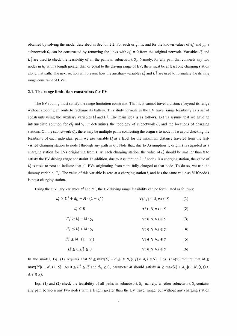
Figure 1. An example to illustrate the EV driving range constraint
Using the example shown in Figure 1, we illustrate how Eqs. (1)-(6) verify the EV travel range feasibility. In
this example, node A is the origin and node E is the destination. Assume that a solution assigns node D to be the
only charging station (i.e., 1, and 0), and that EVs can travel on any link in the network
(i.e., 1). Note that the charging station location (i.e., variable ) and whether EVs
can travel on a link (i.e., variable ), are decision variables that should satisfy the EV travel range feasibility
defined by Eq. (1)-(6). This example, however, focuses on whether the given values of and can satisfy Eq. (1)-
(6). In Figure 1, the number in the middle of a link denotes its distance. There are two labels within the parentheses
for each node. The first label is and the second label is .
and are determined according to Eqs. (1)-(6), as follows. At any node except charging station D,
due to Eqs. (3) and (4). For any node i in the network, tracks the maximum distance traveled from origin A or
charging station D to node using Eq. (1). The only difference between and is at charging station D, where
is zero, while tracks the maximum distance from origin to charging station D. Eq. (2) assesses whether the
9
maximum distance from the last-visited charging station, or from origin, satisfies the EV driving range bound. At
node E, is 5; it tracks the distance traveled from charging station D using according to Eq. (1). Based on the
values of and in Figure 1, if EV driving range R is 12, then the current solution (i.e., 1,
0, and 1) is feasible, and satisfies the EV driving range constraint.
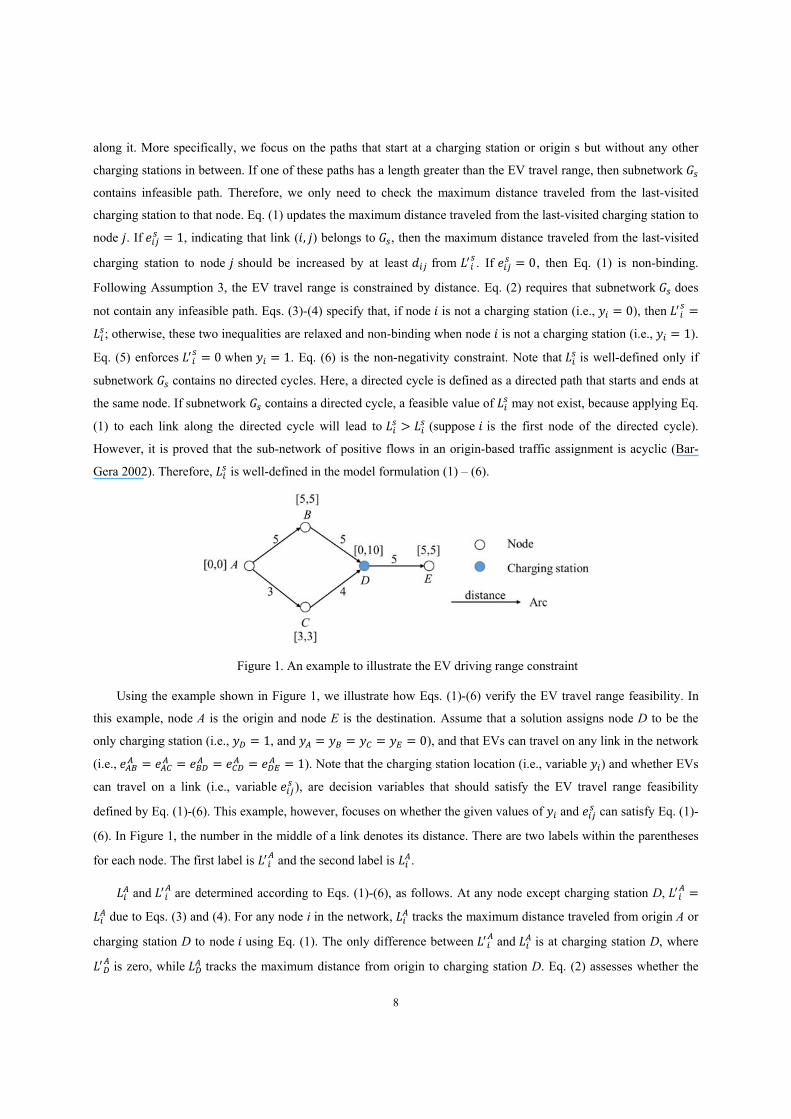
If EV driving range is 8, we can observe that in Figure 1 is larger than EV driving range. It violates Eq. (2).
The current solution (i.e., 1, 0, and 1) is infeasible.
Either or should be zero to satisfy the EV driving range constraint, such that no EVs can travel on path A-B-
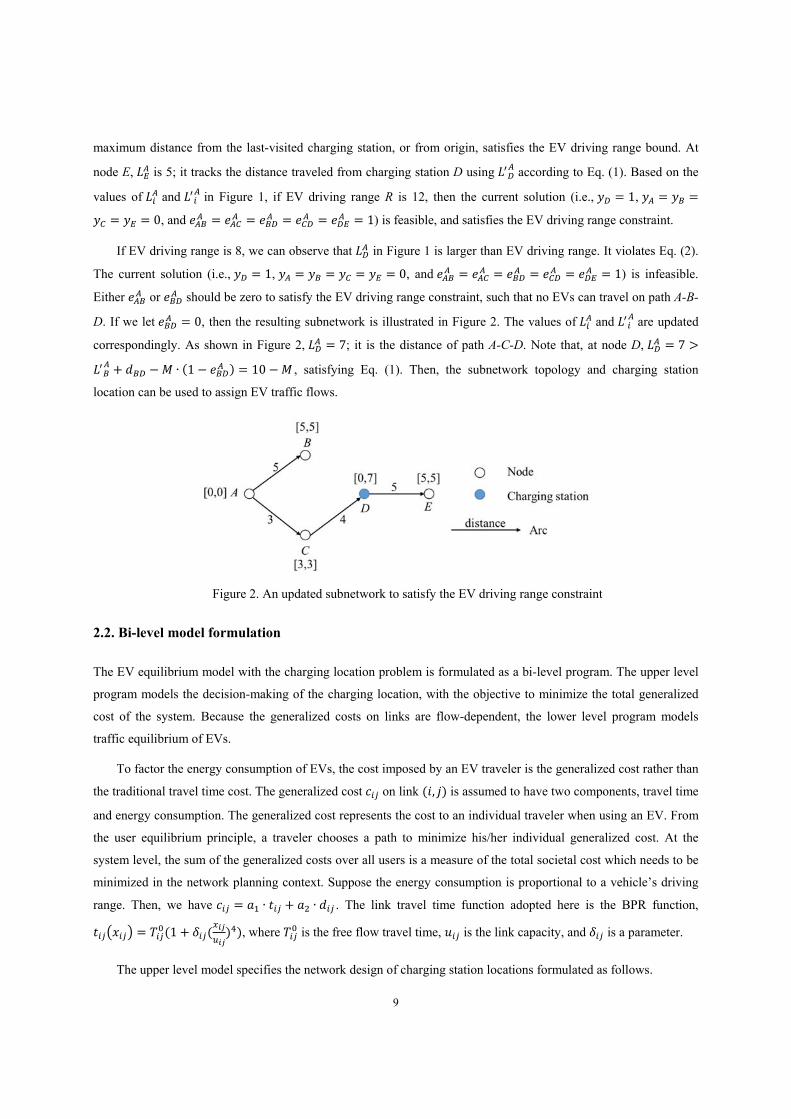
D. If we let 0, then the resulting subnetwork is illustrated in Figure 2. The values of and are updated
correspondingly. As shown in Figure 2, 7; it is the distance of path A-C-D. Note that, at node D, 7
∙ 1 10 , satisfying Eq. (1). Then, the subnetwork topology and charging station
location can be used to assign EV traffic flows.
Figure 2. An updated subnetwork to satisfy the EV driving range constraint
2.2. Bi-level model formulation
The EV equilibrium model with the charging location problem is formulated as a bi-level program. The upper level
program models the decision-making of the charging location, with the objective to minimize the total generalized
cost of the system. Because the generalized costs on links are flow-dependent, the lower level program models
traffic equilibrium of EVs.
To factor the energy consumption of EVs, the cost imposed by an EV traveler is the generalized cost rather than
the traditional travel time cost. The generalized cost on link , is assumed to have two components, travel time
and energy consumption. The generalized cost represents the cost to an individual traveler when using an EV. From
the user equilibrium principle, a traveler chooses a path to minimize his/her individual generalized cost. At the
system level, the sum of the generalized costs over all users is a measure of the total societal cost which needs to be
minimized in the network planning context. Suppose the energy consumption is proportional to a vehicle’s driving
range. Then, we have ∙ ∙ . The link travel time function adopted here is the BPR function,
1 , where is the free flow travel time, is the link capacity, and is a parameter.
The upper level model specifies the network design of charging station locations formulated as follows.

10
min,
∙, ∈
∙ ∙, ∈
∙ ∙, ∈
(7)
s.t.
∈
∙ ∀ ∈ (8)
∙ ∀ , ∈ , ∀ ∈ (9)
∈
∀ , ∈ (10)
and Eqs. (1) – (6)
∈ 0,1 ∀ , ∈ (11)
∈ 0,1 ∀ ∈ (12)
where is the solution of the lower level model, which is the traffic equilibrium with respect to the generalized
cost. At user equilibrium state, no EV can reduce its generalized cost by unilaterally changing path. The decision
variable in the lower level model is the origin-based flow. We formulate the multi-commodity flows through
origin-based flows because they contain path-based information without requiring explicit path enumeration. Further,
with origin-based flows, Eqs. (1) – (6) are well-defined because links with 0 (or 1) do not form a
directed cycle. Note that we can set parameter to be greater than the largest origin-destination demand in Eq. (9).
The user equilibrium state is obtained subject to the charging station locations determined by the upper level
model. Since EVs must satisfy the range limitation constraint in the upper level model (Eqs. (1) – (6)), the
equilibrium condition is achieved among a subset of paths which are range feasible. He et al. (2014) model the
equilibrium among a set of range-feasible paths by enumerating paths; however, we model it through a link-node
representation without path enumeration by using origin-based flows. Eqs. (13)–(16) formulate the traffic
equilibrium in the lower level model.
min, ∈
(13)
s.t.
, ∈ , ∈
∀ ∈ , ∀ ∈ (14)
∈
∀ , ∈ (15)
0 ∀ , ∈ , ∀ ∈ (16)
Next, we discuss how to formulate the KKT conditions of the lower level model to transform the bi-level
program into a single level model.
11
2.3. Single level model formulation
Since the lower level model is a convex mathematical program (Bar-Gera 2002), due to strict convexity of the
objective function with respect to link flows, the KKT conditions are both necessary and sufficient for the optimality
of link flows. Let be the dual variable associated with Eq. (14). represents the minimum cost to travel from
root to node ∈ . The following set of KKT conditions satisfies user equilibrium.
∙ 0 ∀ , ∈ , ∀ ∈ (17)
0 ∀ , ∈ , ∀ ∈ (18)
and Eqs. (14) – (16)
Recall that is the generalized cost which has the form of ∙ ∙ . Deonte by
the reduced cost of link , for commodity . Then, the KKT condition becomes the
following well-known reduced cost optimality condition.
∙ 0 ∀ , ∈ , ∀ ∈ (19)
0 ∀ , ∈ , ∀ ∈ (20)
and Eqs. (14) – (16)
Eq. (19) involves a nonlinear term. By using the auxiliary variable ∈ 0,1 , one can linearize (19) as follows
(Farvaresh and Sepehri 2011).
∙ ∀ , ∈ , ∀ ∈ (21)
1 ∙ ∀ , ∈ , ∀ ∈ (22)
∈ 0,1 ∀ , ∈ , ∀ ∈ (23)
The set of linear constraints (14) – (16), (20) – (23) specifies the optimality condition of the equilibrium model,
which ensures the optimal solution in the lower level model. Thus, we include the set of constraints (14) – (16), (20)
– (23) in the upper level model to transform the bi-level program into a single level program. Note that we can set
to be greater than the largest origin-destination demand in Eq. (21), and to be greater than the total distance of all
links in the network in Eq. (22).
2.4. Simplification of the model
The link travel time function is the BPR function which involves a nonlinear term with respect to variable . In
order to have a convex and linear function to facilitate the solution algorithm, we approximate the link travel time
function by a set of piecewise linear functions. The convex travel time curve is partitioned into sub-intervals
, , where each sub-interval is linear. The slope of the kth sub-interval is . The flow

12
variable can be represented by ∑ , and ∑ , where represents the free
flow travel time on link , .
There is one implicit constraint,
0 ⇒ ∀ 0,1,… , 1, ∀ , ∈ (24)
To enforce constraint (24), we need to introduce a set of binary variables as follows. Let ∈ 0,1 and ∈ 0,1 .
We transform the piecewise linear function into the following equivalent mixed integer linear constraints.
∀ 0,1,… , , ∀ , ∈ (25)
1 ∀ 0,1,… , , ∀ , ∈ (26)
1 ∀ 0,1, … , 1, ∀ , ∈ (27)
where is a small positive constant number, and is a very large positive constant number. Here, can be set to
be greater than . Eq. (25) specifies 0 ⇒ 0 , and 1 ⇒ . Eq. (26)
implies 0 ⇒ 0, and 1 ⇒ 0. Finally, Eq. (27) states that:
0, 1 ⇒ 0,
1, 0 ⇒ 0, 0
which is equivalent to Eq. (24).
The objective function of the upper level problem still involves a nonlinear term ∙ with respect to
variable . However, this nonlinear term can be rewritten as a linear term in terms of variable (Farvaresh and
Sepehri 2011). denotes the minimum travel cost from root to node . Thus, the objective function can be
rewritten as follows.
∙, ∈ ∈ \∈
∙ (28)
We incorporate the KKT condition of the equilibrium model in the lower level problem into the upper level
problem. The resulting single level model formulation is as follows.
min, , , ,
∈ \∈
∙
(29)
s.t. ∈
∙ ∀ ∈ (30)
∙ ∀ , ∈ , ∀ ∈ (31)
∙ 1 ∀ , ∈ , ∀ ∈ (32)
∙ ∀ ∈ , ∈ (33)
∙ ∀ ∈ , ∈ (34)
∀ ∈ , ∀ ∈ (35)
13
∙ 1 ∀ ∈ , ∀ ∈ (36)
: , ∈ : , ∈
∀ ∈ , ∀ ∈ (37)
∈
∀ , ∈ (38)
∀ , ∈ (39)
∀ , ∈ (40)
∙ ∙ ∀ , ∈ (41)
1 ∙ ∀ , ∈ ,∀ ∈ (42)
∀ , ∈ , ∀ 1,2,… , (43)
∀ 0,1, … , , ∀ , ∈
(44)
1 ∀ 0,1, … , , ∀ , ∈
(45)
1 ∀ 0,1, … , 1,
∀ , ∈ (46)
0 ∀ ∈ (47)
0 ∀ , ∈ ,∀ ∈ (48)
0 ∀ , ∈ ,∀ ∈ (49)
0 ∀ , ∈ ,∀ ∈ (50)
0 ∀ ∈ , ∀ ∈ (51) 0 ∀ ∈ , ∀ ∈ (52)
∈ 0,1 ∀ , ∈ (53)
∈ 0,1 ∀ ∈ (54)
∈ 0,1 ∀ 0,1,… , , ∀ , ∈ (55)
∈ 0,1 ∀ 0,1,… , , ∀ , ∈ (56)
Problem (29) – (56) is the EV charging location problem with equilibrium constraints; it is a mixed integer
linear program. The commercial solver CPLEX is used to solve it for the numerical example in the next section.
3. Numerical example
A numerical example is used to analyze the proposed model. The EV charging location problem with traffic
equilibrium is solved for the Sioux Falls network, which consists of 24 nodes and 76 links. To keep the
computational burden reasonable, the number of origins is limited to 3, and no restriction is placed on the number of
destinations. Hence, the number of origin-destination pairs is 3*24 = 72. The network and demand are obtained from
the website of Transportation Test Problems at http://www.bgu.ac.il/~bargera/tntp/. The free flow speed, link
distance and link capacity, as well as parameters of the BPR function, are identical to the network provided by the
website. In this example, suppose the maximum range of EVs is 10. Nodes 1, 2 and 3 are the three origins. All 24
nodes are candidates for charging stations. The construction cost is tabulated in Table 1. The maximum budget for
the construction of charging stations is 25,000. In the example, we choose 0.5 and 0.5.

14
The model contains 448 binary variables after pre-processing. The problem is solved using CPLEX 12.1
interfaced with Python 2.7 on a personal computer equipped with a 2.66-GHz Intel(R) Xeon(R) E5640 CPU with 24
GB of memory. It takes 95.4 minutes to solve to optimality.
Table 1. Construction costs of candidate charging stations
Node Construction
cost Node
Construction cost
Node Construction
cost
1 7960 9 5131 17 2339
2 2790 10 6517 18 2568
3 1204 11 6440 19 993
4 7466 12 1389 20 6694
5 1170 13 7141 21 9742
6 6815 14 6127 22 8496
7 5457 15 8684 23 1654
8 4206 16 3076 24 2620
Table 2. Equilibrium flows on links (veh/h)
Link Flow Link Flow Link Flow
1-2 3100 5-9 2400 16-10 600
1-3 6300 6-5 800 16-17 1200
2-1 600 6-8 5400 17-19 500
2-6 6300 7-18 300 18-20 200
3-1 200 8-7 1100 19-15 100
3-4 4604.16 8-16 2900 20-22 100
3-12 4095.84 11-14 916.18 21-20 300
4-11 804.16 12-11 1112.02 21-22 683.82
4-5 3400 12-13 2483.82 22-15 183.82
5-4 500 13-24 1583.82 24-21 1083.82
5-6 900 14-15 416.18 24-23 400
In the optimal solution, 9 charging stations are selected, as shown in Figure 3. The total construction cost is
23,673 which is less than the budget of 25,000. The corresponding equilibrium flows are reported in Table 2. The
total generalized cost is 235819.55. The travel distances by visiting the charging stations ( ) are reported in Table 3.
It is easy to verify that does not exceed the travel range of 10 in the example.

15
1 2
3 4 5 6
8 79
101112 16 18
17
191514
23 22
2124 2013
Figure 3. Sioux Falls network and the selected charging stations
Table 3. Values of solved for using the model
Origin 1 Origin 2 Origin 3 Node Node Node
1 0 1 6 1 4 2 6 2 0 2 10 3 6 3 10 3 0 4 4 4 2 4 4 5 6 5 9 5 6 6 5 6 5 6 4 7 3 7 3 7 3 8 10 8 10 8 6 9 5 9 5 9 5 10 8 10 9 10 8 11 10 11 8 11 6 12 4 12 4 12 4 13 3 13 3 13 3 14 5 14 4 14 4 15 10 15 5 15 8 16 5 16 5 16 5 17 7 17 7 17 7 18 5 18 5 18 0 19 2 19 2 19 0 20 9 20 4 20 0 21 3 21 0 21 3 22 5 22 9 22 5 23 2 23 0 23 2 24 7 24 0 24 10

16
1 2
3 4 5 6
8 79
101112 16 18
17
191514
23 22
2124 2013
Legend: Road
Node Charging station
6
4 5
4 2 4
4 6
5 2
10
3 5
3
2
6 5 4 3
3
4
4
4
2
6
8
2
2
5
4
3
3
2
3
4
5
6
4
distance Road utilized in equilibrium flow
Figure 4. Equilibrium flows and range limitation verification for paths of Origin 1
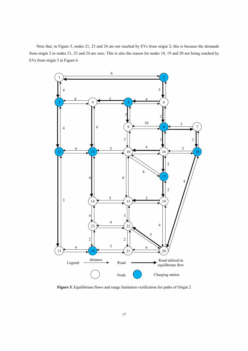
The equilibrium flows for origins 1 to 3 are plotted in Figures 4 to 6, respectively. Bolded links indicate that
they are used, i.e., 0 or 1. The distance of links is also plotted in the figures. It can be verified that in the
equilibrium flow every utilized path satisfies the range limitation condition, i.e., an EV must stop to recharge before
it exceeds the range of 10.
17
Note that, in Figure 5, nodes 21, 23 and 24 are not reached by EVs from origin 2; this is because the demands
from origin 2 to nodes 21, 23 and 24 are zero. This is also the reason for nodes 18, 19 and 20 not being reached by
EVs from origin 3 in Figure 6.
1 2
3 4 5 6
8 79
101112 16 18
17
191514
23 22
2124 2013
Legend: Road
Node Charging station
6
4 5
4 2 4
4 6
5 2
10
3 5
3
2
6 5 4 3
3
4
4
4
2
6
8
2
2
5
4
3
3
2
3
4
5
6
4
distance Road utilized in equilibrium flow
Figure 5. Equilibrium flows and range limitation verification for paths of Origin 2

18
1 2
3 4 5 6
8 79
101112 16 18
17
191514
23 22
2124 2013
Legend: Road
Node Charging station
6
4 5
4 2 4
4 6
5 2
10
3 5
3
2
6 5 4 3
3
4
4
4
2
6
8
2
2
5
4
3
3
2
3
4
5
6
4
distance Road utilized in equilibrium flow
Figure 6. Equilibrium flows and range limitation verification for paths of Origin 3
4. Conclusions
This paper addresses the EV traffic equilibrium and optimal deployment of charging locations subject to the range
limitation. The structure of the problem is similar to the bi-level model of network design problem with traffic
equilibrium. The upper level model is a network design problem to optimally locate charging stations such that the
total generalized cost is minimized. The lower level problem models travelers’ path choice decisions, in which each

19
traveler minimizes his/her individual generalized cost. The generalized cost is composed of travel time and energy
consumption; the latter is proportional to the travel distance. All utilized paths have identical generalized costs, and
satisfy the range limitation constraint. Note that the objectives of the problems in the two levels do not align, and
often conflict, with each other. To obtain the global optimal solution, a single level model is formulated by adding
the optimality condition of the lower level model to the upper level problem. The nonlinear link travel time function
is approximated by piecewise linear functions, enabling the problem to be formulated as a mixed integer linear
program that can be solved using off-the-shelf commercial software.
In contrast to the shortest path problem and the network design problem with relays studied by the operations
research community, our problem is more complicated as it models flow-dependent cost in traffic equilibrium. The
traffic equilibrium is enabled on top of range feasibility specified by the upper level network design problem, i.e., all
utilized paths are range feasible and have equal and minimum generalized cost. In previous studies (He et al. 2014),
range-feasible paths are equilibrated using path enumeration. In this regard, we use origin-based flows in the multi-
commodity flow model formulation to equilibrate range-feasible paths in a link-node representation of the network
without explicit path enumeration. This is because the origin-based flows contain some path information in the
traffic equilibrium but do not necessarily require path enumeration. This property enables us to formulate the EV
travel range constraint on a set of subnetworks containing feasible paths, and circumvent the time-consuming task of
verifying the travel range constraint on each individual path.
For the Sioux Falls network example, it has been verified that the model can solve for the equilibrium flow
combined with the optimal deployment of charging locations. In particular, it has been numerically verified that all
utilized paths are equilibrated while satisfying the range limitation condition.
In this study, using CPLEX, it takes about 95 minutes to reach optimality for the Sioux Falls network with three
origins. Though the global solution is obtained, the computational time is significant for a network of modest size
(with about 400 binary variables). With increased problem size, the computational time may increase substantially.
Hence, there is a need to explore efficient solution algorithms to apply the proposed model to large-scale networks.
Acknowledgements
This research is based on the funding provided by the U.S. Department of Transportation through the NEXTRANS
Center, the USDOT Region 5 University Transportation Center, and partly supported by the National Natural
Science Foundation of China (Grant No.61304197), and the Scientific and Technological Talents Project of
Chongqing (Grant No. cstc2014kjrc-qnrc30002). The authors are solely responsible for the contents of this paper.
References
Adler, J. D., Mirchandani, P. B., Xue, G., and Xia, M. (2016). "The electric vehicle shortest-walk problem with battery exchanges." Networks and Spatial Economics, 16(1), 155-173.
Bar-Gera, H. (2002). "Origin-based algorithm for the traffic assignment problem." Transportation Science, 36(4), 398-417.

20
Beasley, J. E., and Christofides, N. (1989). "An algorithm for the resource constrained shortest path problem." Networks, 19(4), 379-394.
Ben-Ayed, O., and Blair, C. E. (1990). "Computational difficulties of bilevel linear programming." Operations Research, 38(3), 556-560.
Botsford, C., and Szczepanek, A. (2009). "Fast charging vs. slow charging: pros and cons for the new age of electric vehicles." EVS 24, Stavanger, Norway.
Boyce, D. E. (1984). "Urban transportation network equilibrium and design models: recent achievements and future prospectives." Environment and Planning A, 16(11), 1445-1474.
Cabral, E. A., Krkut, E., G., L., and Patterson, R. A. (2007). "The network design problem with relays." European Journal of Operational Research, 180(2), 834-844.
Farahani, R. Z., Miandoabchi, E., Szeto, W. Y., and Rashidi, H. (2013). "A review of urban transportation network design problems." European Journal of Operational Research, 229(2), 281-302.
Farvaresh, H., and Sepehri, M. M. (2011). "A single-level mixed integer linear formulation for a bi-level discrete network design problem." Transportation research Part E: Logistics and Transportation Review, 47(5), 623-640.
Fontaine, P., and Minner, S. (2014). "Benders decomposition for discrete-continuous linear bilevel problems with application to traffic network design." Transportation Research Part B: Methodological, 70, 163-172.
Freisz, T. L. (1985). "Transportation network equilibrium, design and aggregation: key developments and research opportunities." Transportation Research Part A: General, 19(5-6), 413-427.
Friesz, T. L., Cho, H.-J., Mehta, N. J., Tobin, R. L., and Anandalingam, G. (1992). "A simulated annealing approach to the network design problem with variational inequality constraints." Transportation Science, 26(1), 18-26.
He, X., and Peeta, S. (2014). "Dynamic resource allocation problem for transportation network evacuation." Networks and Spatial Economics, 14(3-4), 505-530.
He, F., Yin, Y., and Lawphongpanich, S. (2014). "Network equilibrium models with battery electric vehicles." Transportation Research Part B: Methodological, 67, 306-319.
He, F., Yin, Y., Wang, J., and Yang, Y. (2016). "Optimal prices of electricity at public charging stations for plug-in electric vehicles." Networks and Spatial Economics, doi:10.1007/s11067-013-9212-8.
Hodgson, M. J. (1990). "A flow capturing location-allocation model." Geographical Analysis, 22(3), 270-279. Huang, Y., Li, S., and Qian, Z. S. (2015). "Optimal deployment of alternative fueling stations on transportation
networks considering deviation paths." Networks and Spatial Economics, 15(1), 183-204. Jiang, N., and Xie, C. (2014). "Computing and analyzing mixed equilibrium network flows with gasoline and
electric vehicles." Computer-Aided Civil and Infrastructure Engineering, 29(8), 626-641. Jiang, N., Xie, C., and Waller, S. T. (2012). "Path-constrained traffic assignment: model and algorithm."
Transportation Research Record: Journal of the Transportation Research Board, 2283, 25-33. Karoonsoontawon, A., and Waller, S. T. (2006). "Dynamic continuous network design problem: linear bilevel
programming and metaheuristic approaches." Transportation Research Record: Journal of the Transportation Research Board, 1964, 104-117.
Konak, A. (2012). "Network design problem with relays: A genetic algorithm with a path-based crossover and a set covering formulation." European Journal of Operational Research, 218(3), 829-837.
Kuby, M., and Lim, S. (2005). "The flow-refueling location problem for alternative-fuel vehicles." Socio-Economic Planning Sciences, 39(2), 125-145.
Kuby, M., and Lim, S. (2007). "Location of alternative-fuel stations using the flow-refueling location model and dispersion of candidate sites on arcs." Networks and Spatial Economics, 7(2), 129-152.
Laporte, G., and Pascoal, M. M. B. (2011). "Minimum cost path problems with relays." Computers & Operations Research, 38, 165-173.
Lin, D. Y., Karoonsoontawong, A., and Waller, S. T. (2011). "A Dantzig-Wolfe decomposition based heuristic scheme for bi-level dynamic network design problem." Networks and Spatial Economics, 11(1), 101-126.
Luathep, P., Sumalee, A., Lam, W. H., Li, Z.-C., and Lo, H. K. (2011). "Global optimization method for mixed transportation network design problem: a mixed-integer linear programming approach." Transportation Research Part B: Methodological, 45(5), 808-827.
Magnanti, T. L., and Wong, R. T. (1984). "Network design and transportation planning: models and algorithms." Transportation Science, 18(1), 1-55.
Meng, Q., and Yang, H. (2002). "Benefit distribution and equity in road network design." Transportation Research Part B: Methodological, 36(1), 19-35.
21
Meng, Q., Yang, H., and Bell, M. G. H. (2001). "An equivalent continuously differentiable model and a locally convergent algorithm for the continuous network design problem." Transportation Research Part B: Methodological, 35(1), 83-105.
Mirchandani, P., Adler, J., and Madsen, O. B. G. (2014). "New logistical issues in using electric vehicle fleets with battery exchange infrastructure." Procedia - Social and Behavior Sciences, 108, 3-14.
Mock, P., Schmid, S., and Friendrich, H. (2010). "Market prospects of electric passenger vehicles." In: Electric and Hybrid Vehicles: Power Sources, Models, Sustainability, Infrastructure and the Market, G. Pistoia, ed., Elsevier, Amsterdam, Netherlands.
Ogden, J. M., Steinbugler, M. M., and Kreutz, T. G. (1999). "A comparison of hydrogen, methanol and gasoline as fuels for fuel cell vehicles: implications for vehicle design and infrastructure development." Journal of Power Sources, 79(2), 143-168.
Poorzahedy, H., and Rouhani, O. M. (2007). "Hybrid meta-heuristic algorithms for solving network design problem." European Journal of Operational Research, 182(2), 578-596.
Senart, A., Kurth, S., Roux, G. L., Antipolis, S., and Street, N. C. (2010). "Assessment framework of plug-in electric vehicles strategies." Smart Grid Communications, 2010 First IEEE International Conference on, 155-160.
Smith, O. J., Boland, N., and Waterer, H. (2012). "Solving shortest path problems with a weight constraint and replenishment arcs." Computers & Operations Research, 39, 964-984.
Tesla Motors. (2014). "www.teslamotors.com." Upchurch, C., Kuby, M., and Lim, S. (2009). "A model for location of capacitated alternative-fuel stations."
Geographical Analysis, 41(1), 85-106. US Department of Energy. (2014a). "http://www.afdc.energy.gov/fuels/electricity_benefits.html." US Department of Energy. (2014b). "www.fueleconomy.gov." Wang, D. Z. W., and Lo, H. K. (2010). "Global optimum of the linearized network design problem with equilibrium
flows." Transportation Research Part B: Methodological, 44(4), 482-492. Wang, Y. W., and Lin, C. C. (2009). "Locating road-vehicle refueling stations." Transportation Research Part E:
Logistics and Transportation Review, 45(5), 821-829. Weaver, L. (2014). "Top three reasons for choosing an electric vehicle."
http://alternativefuels.about.com/od/electricvehicles/a/Top-Three-Reasons-For-Choosing-An-Electric-Vehicle.htm.
Xie, C. and Jiang, N. (2016). Relay requirement and traffic assignment of electric vehicles. Computer-Aided Civil and Infrastructure Engineering, in press.
Xu, T., Wei, H., and Hu, G. (2009). "Study on continuous network design problem using simulated annealing and genetic algorithm." Expert Systems with Applications, 36(2), 1322-1328.
Yang, H., and Bell, M. G. H. (1998). "Models and algorithms for road network design: a review and some new developments." Transport Review, 18(3), 257-278.
Yu, A. S. O., Silva, L. L. C., Chu, C. L., Nascimento, P. T. S., and Camargo, A. S. (2011). "Electric vehicles: struggles in creating a market." In: Technology Management in the Energy Smart World, 1-13.
Zheng, H., and Peeta, S. (2015). "Electric vehicle routing and charging locations for intercity trips." Under review.
View publication statsView publication stats