International Journal of Computer Science and Telecommunications [Volume 5, Issue 8, August 2014] 16

Journal Homepage: www.ijcst.org

Engr. Rashid Farid1 and Junaid Arshad

1

1Department of Computer Science and Engineering, University of Engineering and Technology, Lahore, Pakistan

Abstract— LTE-A is the latest cellular network technology.

LTE-A is the use of heterogeneous networks (HetNets) which

contains combinations of different cells such as of a macro cells

and low power nodes (LPNs). Heterogeneous Network is used to

increase capacity of the system and as well as to increase the

demand for data capacity, especially in hotspot areas where

there is a high density of users. Load balancing is main issue in

urban area, heterogeneous network is used for cell splitting gains

and ensure for user experiences. Cell range extension (CRE) is a

technique that can be used to achieve load balancing in

heterogeneous network. By CRE offset is added to LPNs in cell

selection, which expand the range of LPNs and offload many

users from macro-cells to LPNs. CRE is used for uniform offsets.

The result of uniform offset is not optimal in the load balancing

of heterogeneous network. In this paper, we use the Heuristic

load balancing algorithm which is designed for assigning cell

specific offset LPNs. Heuristic methods are used to speed up the

process of finding a suitable solution. A heuristic algorithm is

used for good quality of load balancing which is close to optimal

solution. By apply the concept of cell load coupling, Range

Optimization framework algorithm is used for cell specific offset.

In this research work, we will implement our algorithm show

results by using MATLAB based Vienna LTE simulator to check

and compare results in different scenario using different offsets

values.

Index Terms– LTE, LTE-A, Heterogeneous Network (HetNets),

LPN and CRE

I. INTRODUCTION

TE (Long Term Evolution) and LTE-A (LTE-Advanced)

are most the latest cellular network technologies. LTE

and LTE-A have a flat, all-IP architecture and all services in

the system are IP-based. We use the 4th

generation system to

reach the limit of the high peak data rates which is 100 Mbps

for the high mobility and 1Gbps for the low mobility [1]?

Heterogeneous Network is the combination of mixed cells

such as macro cells and low power nodes (LPNs) cells. In a

heterogeneous network, low power nodes such as pico cells,

femto cells, and relay nodes are deployed within a macro cell

coverage area. Macro cells have a large node density in a

heterogeneous. By offloading network traffic from the macro

cells to the low power node cell then the data rate capacity

will be increased.

Due to higher transmit power of macro cells; it is difficult

to offload many users in areas with high number of users to

LPNs because a UE will usually select a cell with the highest

received signal power. Many UEs linked with macro-cell

seven if they are placed in the vicinity of the LPNs and the

coverage area of LPNs will be small. LPNs will have low cell

load while macro-cells will have high cell loads.

Due to higher transmit power of macro cells; it is difficult

to offload many users in areas with high number of users to

LPNs because a UE will usually select a cell with the Cell

range expansion (CRE) or cell biasing (CB) is a technique

that can be used to offload more users from macro cells to

LPNs without adding the transmit power of the LPNs. In [2]

high cell biasing (HCB) leads to poor performance of HetNets

by overloading some LPNs. On the other hand Low Cell

Biasing (LCB) not achieves the preferred offloading effect

and macro cells will be overloaded. But for load balancing it

is necessary to select best offsets so as to achieve load

balancing in the HetNet by offloading UEs from macro cells,

in such a manner that it will not lead to overloading LPN

cells. One uniform optimum offset value for all LPNs has

usually been used to achieve a load balancing in the HetNet.

So it is necessary to have cell-specific offsets to achieve an

even higher degree of load balancing.

Evolved Node B (eNodeB) is the hardware that is

connected to the mobile phone network and communicates

directly with mobile handsets (UEs), like a base transceiver

station (BTS) in GSM networks. The design of eNodeB for

LTE depends upon various factors such as number of transmit

and receive antenna elements, linear power amplifier (LPA)

power, radio head configuration tower bottom, tower top or

roof-top, antenna configuration.

A. Goals

Goals of this research paper are:

By adjusting the range of LPN the use of call specific

address has been examined so as to achieve load balancing

in heterogeneous networks. A HetNet in which macro-cells

and LPNs are in a co-channel scenario will be considered.

For Range Optimization we design algorithm and this

algorithm can be used for call specific offset. By this

algorithm we can minimize the call load.

L

Traffic Engineering Based Load Balancing in LTE-A

Heterogeneous Network

ISSN 2047-3338

Engr. Rashid Farid and Junaid Arshad 17

B. Method

First we made the algorithm then Range optimization

framework uses the theory of cell load coupling which will

be made the use of this algorithm

Vienna LTE System Level Simulator is used for simulation.

This simulator involves the creation of a system model for

simulation and simulation scenarios

Jain’s fairness index will be used evaluate the degree of

load balancing.

II. LTE-A AND HETEROGENEOUS NETWORKS

Long Term Evolution (LTE) allows the system to use new

and wider spectrum with higher data rates which

complements the 3G networks. It provides the path towards

fourth generation (4G) cellular networks. LTE Advanced is

capable of peak downloading data rates of about 1 Gbps, with

a wide transmission bandwidth. Current wireless cellular

networks are typically deployed as homogeneous networks

using a macro centric planning process [3]. A homogeneous

cellular system is a network of base stations in a planned

layout and a collection of user terminals.

A. Background of LTE-A Network

Table 1: Background of LTE-A Network

B. LTE-A Key Features

System capacity and efficiency of both the LTE and LTE-A

should be high

LTE bandwidth transmission is flexible which is from 1.4,

3, 5, 7, 10 MHz to up to 20 MHz LTE-A have a very high

data rates and have an even larger bandwidth required.

LTE-A support heterogeneous network deployment,

advanced uplink and downlink spatial multiplexing and

downlink coordinated multipoint (COMP) [4].

Table 2: Comparison of LTE and LTE-A

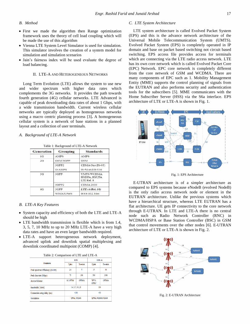
C. LTE System Architecture

LTE system architecture is called Evolved Packet System

(EPS) and this is the advance network architecture of the

Universal Mobile Telecommunication System (UMTS).

Evolved Packet System (EPS) is completely operated in IP

domain and base on packet based switching not circuit based

switching. EPS access file provides access for terminals

which are connecting via the LTE radio access network. LTE

has its own core network which is called Evolved Packet Core

(EPC) Network. EPC core network is completely different

from the core network of GSM and WCDMA. There are

many components of EPC such as 1. Mobility Management

Entity (MME) supports the control planning of signals from

the EUTRAN and also performs security and authentication

tools for the subscribers [5]. MME communicates with the

Home Subscriber Server (HSS) via the S6a interface. EPS

architecture of LTE or LTE-A is shown in Fig. 1.

Fig. 1: EPS Architecture

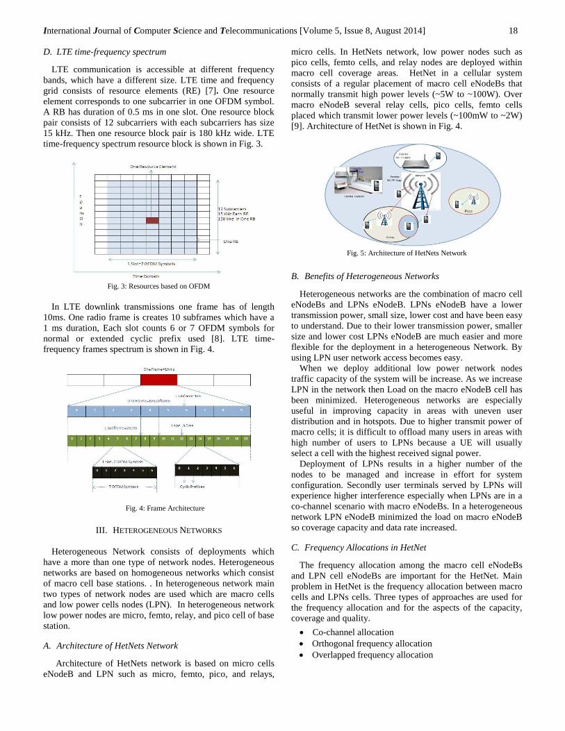
E-UTRAN architecture is of a simpler architecture as

compared to EPS systems because eNodeB (evolved NodeB)

is the only radio access network node or element in the

EUTRAN architecture. Unlike the previous systems which

have a hierarchical structure, whereas LTE EUTRAN has a

flat architecture. UE gets IP connectivity to the core network

through E-UTRAN. In LTE and LTE-A there is no central

node such as Radio Network Controller (RNC) in

WCDMA/HSPA or Base Station Controller (BSC) in GSM

that control movements over the other nodes [6]. E-UTRAN

architecture of LTE or LTE-A is shown in Fig. 2.

Fig. 2: E-UTRAN Architecture

International Journal of Computer Science and Telecommunications [Volume 5, Issue 8, August 2014] 18

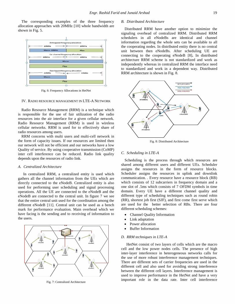
D. LTE time-frequency spectrum

LTE communication is accessible at different frequency

bands, which have a different size. LTE time and frequency

grid consists of resource elements (RE) [7]. One resource

element corresponds to one subcarrier in one OFDM symbol.

A RB has duration of 0.5 ms in one slot. One resource block

pair consists of 12 subcarriers with each subcarriers has size

15 kHz. Then one resource block pair is 180 kHz wide. LTE

time-frequency spectrum resource block is shown in Fig. 3.

Fig. 3: Resources based on OFDM

In LTE downlink transmissions one frame has of length

10ms. One radio frame is creates 10 subframes which have a

1 ms duration, Each slot counts 6 or 7 OFDM symbols for

normal or extended cyclic prefix used [8]. LTE time-

frequency frames spectrum is shown in Fig. 4.

Fig. 4: Frame Architecture

III. HETEROGENEOUS NETWORKS

Heterogeneous Network consists of deployments which

have a more than one type of network nodes. Heterogeneous

networks are based on homogeneous networks which consist

of macro cell base stations. . In heterogeneous network main

two types of network nodes are used which are macro cells

and low power cells nodes (LPN). In heterogeneous network

low power nodes are micro, femto, relay, and pico cell of base

station.

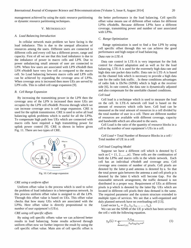
A. Architecture of HetNets Network

Architecture of HetNets network is based on micro cells

eNodeB and LPN such as micro, femto, pico, and relays,

micro cells. In HetNets network, low power nodes such as

pico cells, femto cells, and relay nodes are deployed within

macro cell coverage areas. HetNet in a cellular system

consists of a regular placement of macro cell eNodeBs that

normally transmit high power levels (~5W to ~100W). Over

macro eNodeB several relay cells, pico cells, femto cells

placed which transmit lower power levels (~100mW to ~2W)

[9]. Architecture of HetNet is shown in Fig. 4.

Fig. 5: Architecture of HetNets Network

B. Benefits of Heterogeneous Networks

Heterogeneous networks are the combination of macro cell

eNodeBs and LPNs eNodeB. LPNs eNodeB have a lower

transmission power, small size, lower cost and have been easy

to understand. Due to their lower transmission power, smaller

size and lower cost LPNs eNodeB are much easier and more

flexible for the deployment in a heterogeneous Network. By

using LPN user network access becomes easy.

When we deploy additional low power network nodes

traffic capacity of the system will be increase. As we increase

LPN in the network then Load on the macro eNodeB cell has

been minimized. Heterogeneous networks are especially

useful in improving capacity in areas with uneven user

distribution and in hotspots. Due to higher transmit power of

macro cells; it is difficult to offload many users in areas with

high number of users to LPNs because a UE will usually

select a cell with the highest received signal power.

Deployment of LPNs results in a higher number of the

nodes to be managed and increase in effort for system

configuration. Secondly user terminals served by LPNs will

experience higher interference especially when LPNs are in a

co-channel scenario with macro eNodeBs. In a heterogeneous

network LPN eNodeB minimized the load on macro eNodeB

so coverage capacity and data rate increased.

C. Frequency Allocations in HetNet

The frequency allocation among the macro cell eNodeBs

and LPN cell eNodeBs are important for the HetNet. Main

problem in HetNet is the frequency allocation between macro

cells and LPNs cells. Three types of approaches are used for

the frequency allocation and for the aspects of the capacity,

coverage and quality.

Co-channel allocation

Orthogonal frequency allocation

Overlapped frequency allocation

Engr. Rashid Farid and Junaid Arshad 19

The corresponding examples of the three frequency

allocation approaches with 20MHz [10] whole bandwidth are

shown in Fig. 5.

Fig. 6: Frequency Allocations in HetNet

IV. RADIO RESOURCE MANAGEMENT IN LTE-A NETWORK

Radio Resource Management (RRM) is a technique which

is responsible for the use of fair utilization of the radio

resources into the air interface for a given cellular network.

Radio Resource Management (RRM) is used in wireless

cellular networks. RRM is used for to effectively share of

radio resources among users.

RRM concerns with multi users and multi-cell network in

the form of capacity issues. If our resources are limited then

our network will not be efficient and our networks have a low

Quality of service. By using cooperative transmission (CoMP)

inter cell interference can be reduced. Radio link quality

depends upon the resources of radio link.

A. Centralized Architecture

In centralized RRM, a centralized entity is used which

gathers all the channel information from the UEs which are

directly connected to the eNodeB. Centralized entity is also

used for performing user scheduling and signal processing

operations. All the UE are connected to the eNodeB and the

eNodeB are connected to the central unit. In figure 7 we see

that the entire central unit used for the coordination among the

different eNodeB [11]. Central unit can be used as a bench

mark for performance evaluation. Main overhead which we

have facing is the sending and to receiving of information to

the users.

Fig. 7: Centralized Architecture

B. Distributed Architecture

Distributed RRM have another option to minimize the

signaling overhead of centralized RRM. Distributed RRM

schedulers in all eNodeBs are identical and channel

information regarding the whole sets can be available to all

the cooperating nodes. In distributed entity there is no central

unit between then eNodeBs. After scheduling UE are

connecting to the cooperating eNodeB [8]. In distributed

architecture RRM scheme is not standardized and work as

independently whereas in centralized RRM the interface need

to standardized and work in a dependent way. Distributed

RRM architecture is shown in Fig. 8.

Fig. 8: Distributed Architecture

C. Scheduling in LTE-A

Scheduling is the process through which resources are

shared among different users and different UEs. Scheduler

assigns the resources in the form of resource blocks.

Scheduler assigns the resources in uplink and downlink

communication. . Every resource have a resource block (RB)

which consists of 12 subcarriers in frequency domain and a

one slot of .5ms which consists of 7 OFDM symbols in time

domain. Every UE have a different channel quality and

different type of scheduling techniques such as round robin

(RR), shortest job first (SJF), and first come first serve which

are used for the better selection of RBs. There are four

different scheduling schemes:

Channel Quality Information

Link adaptation

Power allocation

Buffer Information

D. RRM techniques in LTE-A

HetNet consist of two layers of cells which are the macro

cell and the low power nodes cells. The presence of high

inter-layer interference in heterogeneous networks calls for

the use of more robust interference management techniques.

There are different sets of carrier frequencies are used in the

different cell and also used for avoiding strong interference

between the different cell layers. Interference management is

used to improve performance in the HetNet and have a very

important role in the data rate. Inter cell interference

International Journal of Computer Science and Telecommunications [Volume 5, Issue 8, August 2014] 20

management achieved by using the static resource partitioning

or dynamic resource partitioning techniques.

V. METHODOLOGY

A. Load Balancing Introduction

In cellular network main problem we have facing is the

load imbalance. This is due to the unequal allocation of

resources among the users. Different users are connected to

different cells and every cell has a different power, range and

capacity. First of all we see that this load imbalance is due to

the imbalance of power in macro cells and LPN. Due to

power unbalancing small amount of user are connected to

LPN. When few users are associated with LPN eNodeB then

LPN eNodeB have very low cell as compared to the macro

cell. So Load balancing between macro cells and LPN cells

can be achieved by expanding the coverage area of LPNs.

When coverage area is increased then more UEs are served by

LPN cells. This is called cell range expansion [9].

B. Cell Range Expansion

By increasing the transmitting power in the LPN then the

coverage area of the LPN is increased then more UEs are

occupies by the LPN cell eNodeB. Process through which we

can increase coverage area is cell range expansion. CRE is

used for the uplink transmission. CRE is used to solve all load

balancing uplink problems which is useful for all the LPNs.

To compensate high path loss UEs which are connected with

macro cells have required a high transmitting power for

uplink power control [9]. CRE is shown in below given

Fig. 11. There are two types of CRE.

Fig. 10: Cell range expansion

CRE using a uniform offset

Uniform offset value is the process which is used to solve

the problem of load imbalance in a heterogeneous network. In

this process uniform offset value is assigned to all the LPN.

Through this offset value is based on UEs. This offset value

checks that how many UEs which are associated with the

LPNs. Here offset value is directly propositional to the

number of user equipment’s (UEs).

CRE using cell specific offsets

By using cell specific offsets value we can achieved better

results in load balancing. Some results achieved through

uniform offset now we further improve the result by using the

cell specific offset value. Main aim of cell specific offset is

the better performance in the load balancing. Cell specific

offset value means use of different offset values for different

LPNs eNodeBs. Because different LPNs have a different

coverage, transmitting power and number of user associated

with LPNs.

C. Range Optimization

Range optimization is used to find a fine LPN by using

cell specific offset through this we can achieve the good

performance and high output of load balancing.

Data rate in LTE-A

Data rate control in LTE-A is very important for the link

control for channel adaptation and as well as for the load

balancing. LTE-A is used for the extremely high data rate and

high data rate packet data traffic. Data rate in LTE-A is based

on the channel link which is necessary to provide a high data

rate for the radio link traffic. . In these conditions advantages

of radio link is Eb/No (SINR) which is high at the receiver

side [6]. In rate control, the data rate is dynamically adjusted

and also compensate for the unreliable channel conditions.

Cell load

Cell load is a technique which is used to measure the load

on the cell. In LTE-A network cell load is based on the

amount of resources which cells have. Cell load can be

measured as the total amount of resources in a cell divided by

the total number of user in a cell. There are different number

of resources are available with different coverage, capacity

and bandwidth which are allocated to the users.

Cell Load is the ratio of the quantity of resource blocks in a

cell to the number of user equipment’s UEs in a cell.

Cell Load = Total Number of Resource Blocks in a cell /

Total number of UE in a cell

Cell load Coupling Model

Suppose we have a different cell which is denoted by

such as = {1, 2........, }. These cells are the combination of

both the LPNs and macro cells in the whole network. Each

cell has an individual eNodeB and coverage area. Cell

coverage area consists of number of pixels. Cell pixels are

denoted by the latter and antenna is denoted by . So that

the total power gain between the antenna and cell pixels is

denoted by the latter which will become . For the

reasonable network arrangement, the traffic demand is not

distributed in a proper way. Requirement of UEs at different

pixels is which is denoted by the latter . UEs which are

located in different cell pixels their data demand is the same.

The required parameter and the system structure extended to

multiple types of services. We see that a well-organized and

duly planned network have no overloading cell [13].

Load vector . We can see the SINR of the UE which has been served by

the cell with the following equation.

(1)

Engr. Rashid Farid and Junaid Arshad 21

By using Shannon capacity formula high data rate is

achieved for the individual resource block. So that the

Shannon capacity formula by the following formula [13].

(2)

Whereas

is the SNR, in equitation 5.1 SNR of the UE in

a cell is =SNR

(3)

(4)

In equation (4) B is the bandwidth which is used for the

single resource block. Where resource block have a length

180 kHz?

Now we see the number of resource units which are

required to serve demand for pixel which is shown in

the bellow education.

(5)

(6)

In this equation (5) we see that R is the resource blocks in a

cell and is the load on the cell having a pixel [14]. If

we increase bandwidth at 20MHz then the resources will be

increased to 60. Now we have to find the total load in a cell

which is denoted by overall pixels in a cell from equation

(6).

(7)

(8)

(9)

We can see the vector form of the above equation (9) is

shown below. This is general form of cell load coupling.

(10)

If we have N cells then there are N nonlinear equations will

be produced as same as like equation (10). Shortly we write

this above equation as like,

(11)

Now we see the equation cell load coupling for the single

cell.

(12)

For example we have a five cell from the help of above

equation (11) we can write the equation of these five cells as

like this,

(13)

(14)

(15)

(16)

(17)

From equation (9) cell load will be positive if the is not a

zero value.

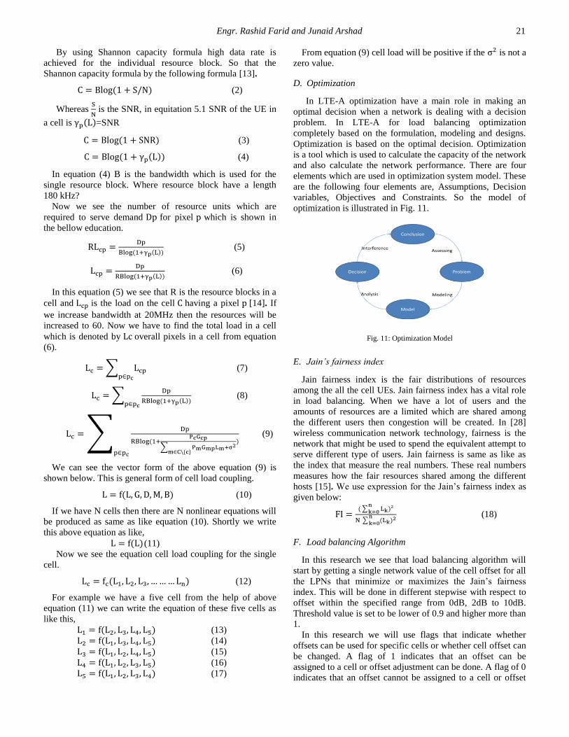
D. Optimization

In LTE-A optimization have a main role in making an

optimal decision when a network is dealing with a decision

problem. In LTE-A for load balancing optimization

completely based on the formulation, modeling and designs.

Optimization is based on the optimal decision. Optimization

is a tool which is used to calculate the capacity of the network

and also calculate the network performance. There are four

elements which are used in optimization system model. These

are the following four elements are, Assumptions, Decision

variables, Objectives and Constraints. So the model of

optimization is illustrated in Fig. 11.

Fig. 11: Optimization Model

E. Jain’s fairness index

Jain fairness index is the fair distributions of resources

among the all the cell UEs. Jain fairness index has a vital role

in load balancing. When we have a lot of users and the

amounts of resources are a limited which are shared among

the different users then congestion will be created. In [28]

wireless communication network technology, fairness is the

network that might be used to spend the equivalent attempt to

serve different type of users. Jain fairness is same as like as

the index that measure the real numbers. These real numbers

measures how the fair resources shared among the different

hosts [15]. We use expression for the Jain’s fairness index as

given below:

(18)

F. Load balancing Algorithm

In this research we see that load balancing algorithm will

start by getting a single network value of the cell offset for all

the LPNs that minimize or maximizes the Jain’s fairness

index. This will be done in different stepwise with respect to

offset within the specified range from 0dB, 2dB to 10dB.

Threshold value is set to be lower of 0.9 and higher more than

1.

In this research we will use flags that indicate whether

offsets can be used for specific cells or whether cell offset can

be changed. A flag of 1 indicates that an offset can be

assigned to a cell or offset adjustment can be done. A flag of 0

indicates that an offset cannot be assigned to a cell or offset

International Journal of Computer Science and Telecommunications [Volume 5, Issue 8, August 2014] 22

cannot be changed. The following variables will be used in

this algorithm:

XPotential network uniform offsets vector

FFlags vector

NumIterOcNumber of iterations required for overloaded

cells’ offsets

NumIterUcNumber of iterations required for under

loaded cells’ offsets.

MaxOffsetMaximum offset that can be applied to cell.

MaxThresholdThreshold value used to determine cell is

overloaded.

Optimal Network offset.

, Optimal cell-specific offsets vector and fairness

index respectively.

Number of iterations NumIterOc and NumIterUc will vary

from network to network. Each cell will collect and send the

necessary load balancing data to the central processing node

for a group of cells through the X2 interface.

Load balancing algorithm

Input X, NumIterNwo, NumIterOc, NumIterUc,

MaxOffset

Output , ,

=0, =0 Ɐ , =1 Ɐ

for k=1: length(X) do

Get optimal network-wide offset

=

If >

End if

End for

=0, Ɐ , = Ɐ

for k=1: NumIterOc do

Deal with overloaded cells

Find overloaded cell

Highest Cell Load = 0

for k=1:length(cells) do

If > MaxThreshold and >0 and >0 Highest Cell

Load

Highest Cell Load =

Highest Cell LoadId = C

end if

end for

y(c)=y(c) - Stepsize

=

>

else

y(c)=y(c) + Stepsize

=0

end if

end for

for k=1: NumIterOc do

Deal with under loaded cells

Find under loaded cell

Lowest Cell Load = 1

for k=1:length(cells) do

If <Lowest Threshold and >0

Lowest Cell Load =

Lowest Cell LoadId = C

end if

end for

y(c)=y(c) + Stepsize

=

>

else

y(c)=y(c) - Stepsize

=0

end if

end for

VI. ANALYSIS AND DESIGN

A. Simulators Introduction

There are various simulators which are used in LTE-A

System for the analysis and design of the system and their

network simulation. We chose that simulator which is better

for us and for LTE simulation and design. We have three

options of simulators such as OPNET Network simulators

(NS), Vienna LTE System Level Simulator.

Vienna LTE Simulator

Vienna LTE system simulates based on two types of

simulation such as Vienna system level simulation and

Vienna link level simulation. Vienna system level simulation

support front end simulation and configure at the physical

layer. Vienna link level simulation used to support a link

between the networks which configure at data link layer of the

network [16]. Vienna LTE System allows for simulation of

not only LTE physical layer but it is possible to relate with

link level issues. In Vienna LTE system physical layer is

abstracted from link level results. By using this simulator we

got high network performance which is beneficial for our

research.

Simulators classes

As we have discussed before, that our simulator has a

modular structure which is programmed as in the form of

object oriented design. Table 3 shows the major packages.

Table 3: Simulator classes

Engr. Rashid Farid and Junaid Arshad 23

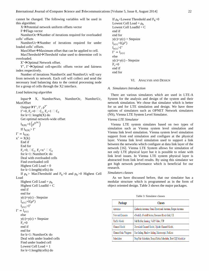
Network layout

These colored are used for their representation in the

network. We see that there are two types of eNodeBs are used

in this network, 1- Macro eNodeBs are represented big sky

blue circles with sectors. 2-LPN eNodeBs are represented big

sky blue circles without sectors. Black circles represent those

users which are not served by any eNodeB. UE color red

served by a Macro cells eNodeBs and UE which have a color

blue served by a LPN cells. Network layout of heterogeneous

network is shown in Fig. 12.

Fig. 12: Heterogeneous Network Layouts

B. Implementation

There are many functions that are used in the simulator

which are used to implement the load balancing algorithm.

We use following functions in the simulator for load

balancing algorithm [17].

Interfering power can be added from the connecting cell.

Another function we use here is the cell load estimation.

This cell load estimation function also makes use of the

array.

We have another function which is used to get those UEs

that are attached to each and every cell. Load balancing

algorithm function.

Function to compute Jain’s fairness index

Function for adding offsets to LPN cells.

These set of equations can be introduced by the

combination of equations that will become summation in

equation (9).

In the equation

where is the demand by UE ,

is the number of resource blocks in the selected bandwidth

and is the bandwidth of that resource block. From our

configuration we used here = 2 , = 70 and = 150

(when we use transmission bandwidth of 15 MHz is

used).

Therefore,

(6.1)

Constant data rate demand is configured using gaming

traffic model. Other factors will vary from UE to UE.

In order to get the optimum value of uniform offset range

the network is simulated from 0 to 12 dB offset in steps of

2dB. The number of iterations for dealing with cells will low

and high cell loads is limited to 15.

C. Simulation Parameters

Simulation Parameters

Parameter Value

System Parameters

Carrier frequency 2 GHz

Thermal noise PSD -174dBm

Penetration loss 20dB eNodeB UE

Pixels resolution 10m/pixel

Bandwidth 20MHz

Inter-eNodeB distance 500m

UE parameters

Antenna configuration 0dBi

UE noise figure 9dB

Maximum transmit power 23dBm

eNodeB Parameters

eNodeB antenna config TX-2,RX-2

eNodeB noise figure 9dB

eNodeB cell transmit power 46dBm

eNodeB antenna gain Directional,14dBi

LPN Parameters

LPN antenna gain Omni-0dBi

LPN noise figure 9dB

LPN transmit power 30dBm

LPN antenna configuration TX-2, RX-2

Traffic model and scheduler

Traffic model Full buffer/Gaming

Scheduler Round robin

VII. SIMULATION RESULTS AND ANALYSIS

We can find performance on the bases of Jain’s fairness

index and UE distribution between the Nodes.

A. Load balancing Result and Estimation

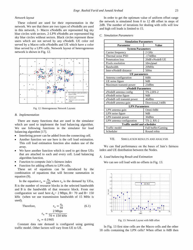
We can see cell load with no offsets in Fig. 13.

Fig. 13: Network Layout with 0dB offset

In Fig. 13 first nine cells are the Macro cells and the other

18 cells containing the LPN cells? When offset is 0dB then

International Journal of Computer Science and Telecommunications [Volume 5, Issue 8, August 2014] 24

most of the LPNs have a very much low load as compared to

Macro cells load. Some LPN has a much low load which is

zero loads. So there is need to increase the range of the LPN

for load balancing among the Macro cell and LPN. LPN cell

which a zero load are the 10, 12, 23 at 0dB.

As the offset is increased from 0 dB, then fairness index

increases steadily and become maximum at 8 dB where

fairness index to drop again as the offset increases from 8 dB

to 12 dB. The load balancing index at 0dB offset is 0.56. It

can be seen from figure 14 that the optimum uniform offset is

8dB. When 8 dB offset is used the resulting load balancing

index is 0.83.

Fig. 14: Comparison of cell load at 0 dB and 8 dB

The fairness index reduce when offset values higher that 8

dB are used because LPNs start to get overloaded. This is

illustrated in figure 15 when a uniform offset of 10 dB is

used.

Fig. 15: Combination of cell load at 0 dB and 10 dB

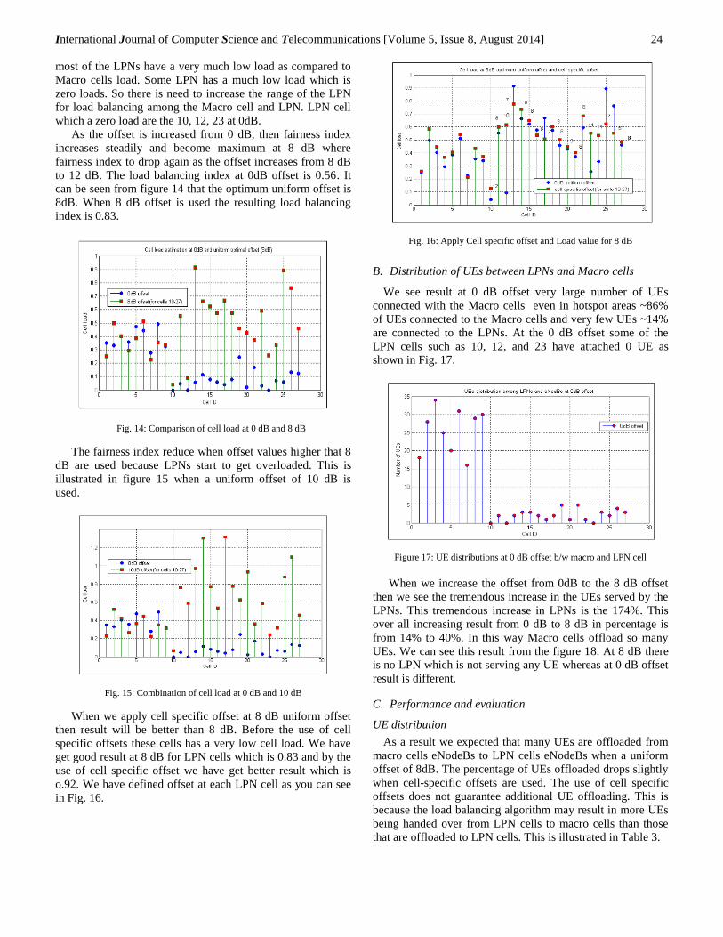
When we apply cell specific offset at 8 dB uniform offset

then result will be better than 8 dB. Before the use of cell

specific offsets these cells has a very low cell load. We have

get good result at 8 dB for LPN cells which is 0.83 and by the

use of cell specific offset we have get better result which is

o.92. We have defined offset at each LPN cell as you can see

in Fig. 16.

Fig. 16: Apply Cell specific offset and Load value for 8 dB

B. Distribution of UEs between LPNs and Macro cells

We see result at 0 dB offset very large number of UEs

connected with the Macro cells even in hotspot areas ~86%

of UEs connected to the Macro cells and very few UEs ~14%

are connected to the LPNs. At the 0 dB offset some of the

LPN cells such as 10, 12, and 23 have attached 0 UE as

shown in Fig. 17.

Figure 17: UE distributions at 0 dB offset b/w macro and LPN cell

When we increase the offset from 0dB to the 8 dB offset

then we see the tremendous increase in the UEs served by the

LPNs. This tremendous increase in LPNs is the 174%. This

over all increasing result from 0 dB to 8 dB in percentage is

from 14% to 40%. In this way Macro cells offload so many

UEs. We can see this result from the figure 18. At 8 dB there

is no LPN which is not serving any UE whereas at 0 dB offset

result is different.

C. Performance and evaluation

UE distribution

As a result we expected that many UEs are offloaded from

macro cells eNodeBs to LPN cells eNodeBs when a uniform

offset of 8dB. The percentage of UEs offloaded drops slightly

when cell-specific offsets are used. The use of cell specific

offsets does not guarantee additional UE offloading. This is

because the load balancing algorithm may result in more UEs

being handed over from LPN cells to macro cells than those

that are offloaded to LPN cells. This is illustrated in Table 3.

Engr. Rashid Farid and Junaid Arshad 25

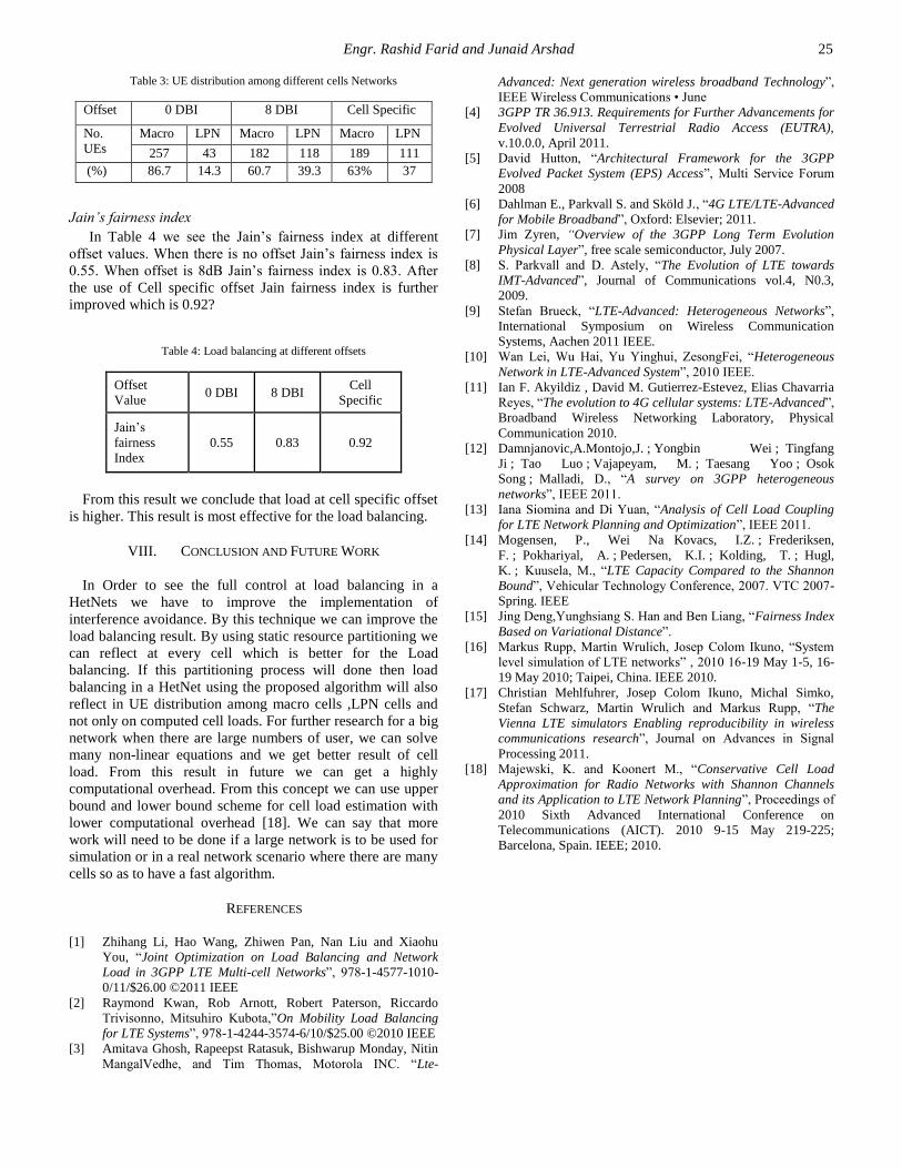
Table 3: UE distribution among different cells Networks

Offset 0 DBI 8 DBI Cell Specific

No.

UEs

Macro LPN Macro LPN Macro LPN

257 43 182 118 189 111

(%) 86.7 14.3 60.7 39.3 63% 37

Jain’s fairness index

In Table 4 we see the Jain’s fairness index at different

offset values. When there is no offset Jain’s fairness index is

0.55. When offset is 8dB Jain’s fairness index is 0.83. After

the use of Cell specific offset Jain fairness index is further

improved which is 0.92?

Table 4: Load balancing at different offsets

Offset

Value 0 DBI 8 DBI

Cell

Specific

Jain’s

fairness

Index

0.55 0.83 0.92

From this result we conclude that load at cell specific offset

is higher. This result is most effective for the load balancing.

VIII. CONCLUSION AND FUTURE WORK

In Order to see the full control at load balancing in a

HetNets we have to improve the implementation of

interference avoidance. By this technique we can improve the

load balancing result. By using static resource partitioning we

can reflect at every cell which is better for the Load

balancing. If this partitioning process will done then load

balancing in a HetNet using the proposed algorithm will also

reflect in UE distribution among macro cells ,LPN cells and

not only on computed cell loads. For further research for a big

network when there are large numbers of user, we can solve

many non-linear equations and we get better result of cell

load. From this result in future we can get a highly

computational overhead. From this concept we can use upper

bound and lower bound scheme for cell load estimation with

lower computational overhead [18]. We can say that more

work will need to be done if a large network is to be used for

simulation or in a real network scenario where there are many

cells so as to have a fast algorithm.

REFERENCES

[1] Zhihang Li, Hao Wang, Zhiwen Pan, Nan Liu and Xiaohu

You, “Joint Optimization on Load Balancing and Network

Load in 3GPP LTE Multi-cell Networks”, 978-1-4577-1010-

0/11/$26.00 ©2011 IEEE

[2] Raymond Kwan, Rob Arnott, Robert Paterson, Riccardo

Trivisonno, Mitsuhiro Kubota,”On Mobility Load Balancing

for LTE Systems”, 978-1-4244-3574-6/10/$25.00 ©2010 IEEE

[3] Amitava Ghosh, Rapeepst Ratasuk, Bishwarup Monday, Nitin

MangalVedhe, and Tim Thomas, Motorola INC. “Lte-

Advanced: Next generation wireless broadband Technology”,

IEEE Wireless Communications • June

[4] 3GPP TR 36.913. Requirements for Further Advancements for

Evolved Universal Terrestrial Radio Access (EUTRA),

v.10.0.0, April 2011.

[5] David Hutton, “Architectural Framework for the 3GPP

Evolved Packet System (EPS) Access”, Multi Service Forum

2008

[6] Dahlman E., Parkvall S. and Sköld J., “4G LTE/LTE-Advanced

for Mobile Broadband”, Oxford: Elsevier; 2011.

[7] Jim Zyren, “Overview of the 3GPP Long Term Evolution

Physical Layer”, free scale semiconductor, July 2007.

[8] S. Parkvall and D. Astely, “The Evolution of LTE towards

IMT-Advanced”, Journal of Communications vol.4, N0.3,

2009.

[9] Stefan Brueck, “LTE-Advanced: Heterogeneous Networks”,

International Symposium on Wireless Communication

Systems, Aachen 2011 IEEE.

[10] Wan Lei, Wu Hai, Yu Yinghui, ZesongFei, “Heterogeneous

Network in LTE-Advanced System”, 2010 IEEE.

[11] Ian F. Akyildiz , David M. Gutierrez-Estevez, Elias Chavarria

Reyes, “The evolution to 4G cellular systems: LTE-Advanced”,

Broadband Wireless Networking Laboratory, Physical

Communication 2010.

[12] Damnjanovic,A.Montojo,J. ; Yongbin Wei ; Tingfang

Ji ; Tao Luo ; Vajapeyam, M. ; Taesang Yoo ; Osok

Song ; Malladi, D., “A survey on 3GPP heterogeneous

networks”, IEEE 2011.

[13] Iana Siomina and Di Yuan, “Analysis of Cell Load Coupling

for LTE Network Planning and Optimization”, IEEE 2011.

[14] Mogensen, P., Wei Na Kovacs, I.Z. ; Frederiksen,

F. ; Pokhariyal, A. ; Pedersen, K.I. ; Kolding, T. ; Hugl,

K. ; Kuusela, M., “LTE Capacity Compared to the Shannon

Bound”, Vehicular Technology Conference, 2007. VTC 2007-

Spring. IEEE

[15] Jing Deng,Yunghsiang S. Han and Ben Liang, “Fairness Index

Based on Variational Distance”.

[16] Markus Rupp, Martin Wrulich, Josep Colom Ikuno, “System

level simulation of LTE networks” , 2010 16-19 May 1-5, 16-

19 May 2010; Taipei, China. IEEE 2010.

[17] Christian Mehlfuhrer, Josep Colom Ikuno, Michal Simko,

Stefan Schwarz, Martin Wrulich and Markus Rupp, “The

Vienna LTE simulators Enabling reproducibility in wireless

communications research”, Journal on Advances in Signal

Processing 2011.

[18] Majewski, K. and Koonert M., “Conservative Cell Load

Approximation for Radio Networks with Shannon Channels

and its Application to LTE Network Planning”, Proceedings of

2010 Sixth Advanced International Conference on

Telecommunications (AICT). 2010 9-15 May 219-225;

Barcelona, Spain. IEEE; 2010.