Embed Size (px)
Citation preview

Traffic Calm
ing in Delhi
-A Feasib
ility S
tudy of
Traffic Safety M
easures
Aalborg University, Denmark, Department of Development and Planning, Final Thesis of Martin Kristian Kallesen


Aalborg University, Denmark
Department of Development and Planning
Final Thesis
M.Sc. in Transportation Engineering
Title:
Traffic Calming in Delhi – a Feasibility Study of Traffic Safety Measures
Tutor:
Professor Christer Hydén, Lund University, Sweden
Number of pages: 139
Aalborg, August 2006
Martin Kristian Kallesen

2 Traffic Calming in Delhi

3
Table of Contents
Summary .................................................................................................................7
Danish Summary....................................................................................................9
Preface....................................................................................................................11
Abbreviations and Notations .............................................................................13
Introduction ..........................................................................................................15
Traffic Safety as a Global Health Problem....................................................15
Traffic Safety in Less Motorized Countries ..................................................19
Technology transfer .........................................................................................21
Chapter 1 Aim and Formulation of Hypotheses .............................................25
1.1 Previous Results with Traffic Calming ............................................25
1.1.1 Traffic Calming in Europe.............................................................25
1.1.2 Traffic Calming in Gothenburg ....................................................26
1.1.3 Experiences from Denmark...........................................................27
1.1.4 Studies about Traffic Calming ......................................................29
1.2 Traffic Safety in India Today.............................................................30
1.3 Formulation of Problem.....................................................................35
1.4 Strategy.................................................................................................36
1.5 Delimitations .......................................................................................36
Chapter 2 Hypothesis Testing ............................................................................39
2.1 How to Test the Hypotheses .............................................................39
2.1.1 Hypothesis 1....................................................................................39
2.1.2 Hypothesis 2....................................................................................39
2.2 Selection of Traffic Sites in Delhi ......................................................40
2.3 Introduction to Selected Sites ............................................................40

4 Traffic Calming in Delhi
2.3.1 Orthonova ....................................................................................... 41
2.3.2 Dilli Haat ......................................................................................... 48
2.4 Methods for Data Collection............................................................. 53
2.4.1 The Swedish Traffic Conflict Technique..................................... 53
2.4.2 A New Severity Scale .................................................................... 58
2.4.3 Speed Measurements..................................................................... 59
2.5 Collected Data..................................................................................... 59
Chapter 3 Data Analysis ..................................................................................... 61
3.1 Analysis Method................................................................................. 61
3.2 Data Analysis - Orthonova ............................................................... 63
3.2.1 Traffic Volumes .............................................................................. 63
3.2.2 Speed................................................................................................ 63
3.2.3 Traffic Conflicts .............................................................................. 64
3.3 Data Analysis - Dilli Haat ................................................................. 67
3.3.1 Traffic Volumes .............................................................................. 67
3.3.2 Speed................................................................................................ 68
3.3.3 Traffic Conflicts .............................................................................. 68
3.4 Data Analysis - General observations ............................................. 71
3.4.1 Physical design ............................................................................... 71
3.4.2 Road User Behaviour..................................................................... 74
3.4.3 Willingness of Risk ........................................................................ 76
3.5 Threshold between conflicts ............................................................. 77
3.6 Diagnosis of Problems ....................................................................... 83
3.6.1 Orthonova ....................................................................................... 83
3.6.2 Dilli Haat ......................................................................................... 83

5
Chapter 4 Results..................................................................................................85
4.1 Existing experiences with traffic conflict technique.......................85
4.2 The Swedish traffic conflict technique .............................................88
4.3 Danish Design Rules of Traffic Calming .........................................90
4.3.1 14 types of traffic calming measures............................................90
4.3.2 Modifications and adaptations .....................................................94
4.4 Proposed Layout at Orthonova ........................................................96
4.5 Proposed Layout at Dilli Haat ........................................................100
4.6 Prognosis of Countermeasures .......................................................102
Chapter 5 Epilogue.............................................................................................105
5.1 Discussion ..........................................................................................105
5.2 Conclusions........................................................................................108
5.3 Perspective .........................................................................................108
5.4 Further studies ..................................................................................109
5.4.1 Bicycle tracks in Delhi..................................................................109
5.4.2 Comparison of willingness of risk .............................................109
5.4.3 Public Transportation ..................................................................109
5.4.4 TCT studies....................................................................................110
References............................................................................................................111
Appendices
Appendix A: Signal Plan for Orthonova
Appendix B: Traffic Conflict Recording Form
Appendix C: Schedule for Field Studies
Appendix D: Traffic Counts at Orthonova

6 Traffic Calming in Delhi
Appendix E: Traffic Counts at Dilli Haat
Appendix F: Speed Measurements at Orthonova
Appendix G: Speed Measurements at Dilli Haat
Appendix H: Example of Conflict Recording Form

Summary
Traffic safety on a global scale is decreasing. The development in high-income countries – like the Nordic countries – is going through an increase in traffic safety in these years, but the global development does not reflect this trend. A comprehensive study made for WHO have showed the expected development in life threatening diseases and injuries between 1990 and 2020. From the ninth highest rank in 1990, traffic injuries are expected to grow into the third biggest threat world wide in 2020.
A number of studies have stressed the connection between countries’ economical income per population and the risk of traffic fatalities (traffic fatalities per population). The development in risk of traffic fatalities most often will be increasing in low- and middle income countries. High-income countries most often will experience a decrease in the risk of traffic fatalities. This report deals with the question whether it is possible to prevent the described increase in risk of traffic fatalities in low- and middle-income countries going through economical growth. One possible measure is transfer of knowledge and techniques from high-income countries – with a high level of traffic safety – to low- and middle-income countries – with a low level of traffic safety. -In this report between the Nordic countries and India aiming at traffic calming measures.
Two hypotheses will be tested. These deal with the possibilities of implementing traffic calming measures in Delhi. In addition it is demonstrated how the Swedish traffic conflict technique is useable in proving the possibilities and effects of technology transfer regarding traffic calming.
Field studies have been made at two traffic sites in Delhi; Orthonova and Dilli Haat. By using the Swedish traffic conflict technique, diagnoses of the occurring problems have been made. A subjective severity scale was developed and used during the observations. It is recommended that a subjective severity scale is used as a supplement to the traffic conflict technique in further conflict studies.

8 Traffic Calming in Delhi
A suggestion for a redesign of Orthonova is being commented. Red light violations should be prevented by an optimization of the signal phases. A suggestion for a redesign of Dilli Haat has been developed and is presented. Traffic calming measures in form of narrowing, prior notice and gateway is used. With the basis in the work at the two locations, a prognosis of traffic calming measures for Delhi has been set up.
The following is concluded as an answer to the two hypotheses:
The Swedish traffic conflict technique is useable in the mixed traffic in Delhi. It was not possible to establish the necessity of a subjective severity scale in order to get useable results. It is however still recommended that such a scale is used as a supplement. It was not possible to point out a new threshold between serious and non-serious conflicts for the traffic in Delhi.
The pedestrian’s conditions are often insufficient in Delhi. Traffic calming measure can be a contributing factor to improve the conditions for the vulnerable road users, like pedestrians.

Danish Summary
Trafiksikkerheden på et globalt plan er faldende. Selv om udviklingen i høj-indkomstlande, som de Nordiske lande, viser en stigning i trafiksikkerhed, er denne tendens ikke at finde globalt. Et omfattende studie udført for WHO har klarlagt den forventede udvikling i livstruende sygdomme eller ulykker mellem 1990 og 2020. Fra at trafikulykker tildeles en niende plads i 1990, vurderes problemet at vokse til at være den tredje mest livstruende sygdom-/ulykkesfaktor på verdensplan i 2020.
Flere studier har påvist en sammenhæng mellem landes økonomiske indkomst per befolkningstal og risikoen for trafikulykker (trafikuheld per befolkningstal). Udviklingen i trafikulykkesrisiko vil oftest være stigende for lav- og middel-indkomstlande, hvorefter den oftest vil falde igen for lande der udvikler sig til høj-indkomstlande. Denne rapport beskæftiger sig med, hvorvidt det er muligt at undgå den beskrevne stigning i ulykkesrisiko for lav- og middelindkomstlande der oplever økonomisk vækst. En metode kan være vidensdeling og teknologioverførsel fra høj-indkomstlande med høj trafiksikkerhed til lav- og middel-indkomstlande med lav trafiksikkerhed. –I denne rapport mellem de Nordiske lande og Indien.
Rapporten omhandler virkemidler af hastighedsdæmpende karakter. To hypoteser vil blive eftervist. Disse omhandler muligheden for implementering af hastighedsdæmpende virkemidler i Delhi. Desuden eftervises det, hvorvidt den svenske trafikkonfliktteknik er anvendelig til at påvise mulighederne for og effekterne af en sådan teknologioverførsel.
I forbindelse med rapporten er der udført feltstudier i Delhi på to lokaliteter. På grundlag af konflikt teknik studier er der lavet diagnoser over de tilstedeværende problemer på de to observerede lokaliteter; Orthonova og Dilli Haat. Der er udarbejdet en subjektiv alvorlighedsskala som er blevet brugt under observationsarbejdet i Delhi. Det anbefales at en sådan skala benyttes som et supplerende værktøj i kommende konflikt studier

10 Traffic Calming in Delhi
Et forslag til ombygning af Orthonova kommenteres. Her nævnes det at rødt lys overtrædelser i særdeleshed bør forebygges ved hjælp af en optimering af signal reguleringens faser. Et forslag til ombygning af Dilli Haat er udarbejdet og præsenteres. Hastighedsdæmpere i form af indsnævring, forvarsel og porte anvendes. På baggrund af arbejdet på de to lokaliteter, er der opstillet en prognose for hastighedsdæmpende tiltag med anvendelse i Delhi.
Der konkluderes følgende, som svar på de to hypoteser:
Den svenske trafikkonfliktteknik er anvendelig i den sammensatte trafik i Delhi. Det er ikke blevet påvist at en subjektiv alvorlighedsskala er nødvendig for at få brugbare resultater, men det anbefales alligevel at anvende en sådan som en sikkerhed for dataenes brugbarhed. Der er ikke fundet grundlag for at kunne påvise en ny grænseværdi mellem alvorlige og ikke-alvorlige konflikter gældende for trafikmiljøet i Delhi.
Fodgængere forhold er ofte mangelfulde i Delhi. Hastighedsdæmpende foranstaltninger kan være medvirkende til at forholdende for bløde trafikanter, som fodgængere, kan forbedres.

Preface
This publication is a final thesis from Aalborg University, Denmark. The report is written with engineers and others with academic interest in the challenges of traffic safety in less industrialised countries in sight. The work on this final thesis has involved a study visit in Delhi, India, as part of the empirical data collection. The report is written in English to enable collaboration with two Indian partners.
The report consists of five chapters and eight appendices. Before chapter 1 the global problems regarding traffic safety are described in the introduction. In chapter 1 the main problem is formulated together with two hypotheses. Chapter 2 gives an explanation on how the hypotheses will be tested. This leads to an introduction of two traffic sites en Delhi which is the basis for the observations. Hereafter the theory of the observation technique is introduced. Chapter 2 ends with a presentation of the collected data from the two traffic sites. Chapter 3 includes the analysis of the collected data. Results regarding traffic conflict technique used in Delhi are presented in chapter 4. This involves, besides the study introduced with this report, a previous study involving traffic conflict technique. With a basis in the results, measures of traffic calming from the Danish design rules are presented. Chapter 4 ends with a prognosis of traffic calming measures for the use in Delhi. Chapter 5 gives a discussion that leads to the final conclusion. Besides, the process regarding the study visit is discussed. To end with, suggestions for further studies are given.
Photos in the report are by the author unless something else is mentioned.
Acknowledgements:
⎯ TRIPP for providing academic help during the time in Delhi. TRIPP were of great significance for the completion of the study visit in Delhi.
⎯ The Volvo Education Research Foundation for facilities provided through TRIPP.

12 Traffic Calming in Delhi
⎯ CUTS for big help with accommodation and giving answers to many practical questions. Especially the people at the Delhi Resource Centre were very helpful during the time in Delhi. CUTS were of great significance for the completion of the study visit in Delhi.
⎯ ManiChowfla (architects and consultants, D 374 defence colony, New Delhi – 110024, India) for their involvement in discussions and help with providing technical drawings.
Abbreviations and Notations
AADT – Average Annual Daily Traffic
Avoiding road user – The road user, in a conflict, that takes evasive action. If both road users do this, then the one that produces the least severe conflict.
Bump – Physical speed reducing measure. Short length compared with a hump.
CDBase – Software tool for a PC to help analyse collected traffic conflict technique data. The software is build upon the theory of the Swedish traffic conflict technique.
CUTS – Consumer Unity and Trust Society. International consumer organisation. One of two local partners in Delhi.
DALYs – Disability Adjusted Life Years. DALYs is an adjusted number of YLL – Years of Life Lost – where it is taken into consideration that a traffic crash victim might survive a crash but live with a disability
Fatality risk – Fatalities per population
HCBS – High Capacity Bus System. In this report it refers to an ongoing project in Delhi.
Hump – Physical speed reducing measure. Long length compared with a bump.
IIT – Indian Institute of Technology in Delhi
Journey speed – the speed of a vehicle hold up by other vehicles and by it has lowered its preferred speed.
14 Traffic Calming in Delhi
Left turn on red – India has left side traffic and it is permitted to make a left turn on red if no other traffic is coming. “Left turn on red” can be compared with the American “right turn on red”.
Mid block (crash) – Between two intersections (crash that happens between two intersections).
MTW – Motorized Two Wheeler. This road user group mostly consists of motorbikes and scooters.
PCU – Private Car Unit. Numbers of MTWs and TSRs – physically smaller than cars – and busses and trucks – physically bigger than cars – can be translated into the same unit size, PCU, and thus be comparable with numbers of person cars.
RU – Road User
Running speed – The speed of a free vehicle that travels by the driver’s preferred speed and not is hold up by other traffic.
Service lane – secondary lane parallel to mainly arterial roads. Small local roads and private drive ways are connected to the service lane. This results in a lower number of intersections on the arterial road. The service lanes are often used for parking.
TA – Time to Accident. The time that remains to a collision, presupposed unchanged speeds and directions.
TCT – Traffic Conflict Technique. The technique used in this study is the Swedish traffic conflict technique.
TRIPP - Transportation Research and Injury Prevention Programme at IIT. TRIPP is a WHO (World Health Organisation) collaborating centre for research and training in safety technology. One of two local partners in Delhi.
TSR – Three wheeled Scooter Rickshaw. This is a local build taxi with three wheels and a scooter engine. The TSR can be compared with the “TUK TUK” from Thailand.
VRU – Vulnerable Road User. This road user group mostly consists of pedestrians, bicyclists and MTWs. Another name is unprotected road user.
WHO – World Health Organization.
Introduction
This introducing chapter will give a broad overview of the traffic safety situation that the world, and in particular developing countries, is facing. There are many ways to address the related problems. One of them is technology transfer from developed countries to developing countries. This specific approach will be described. The question of feasibility of technology transfer is a basis for this report.
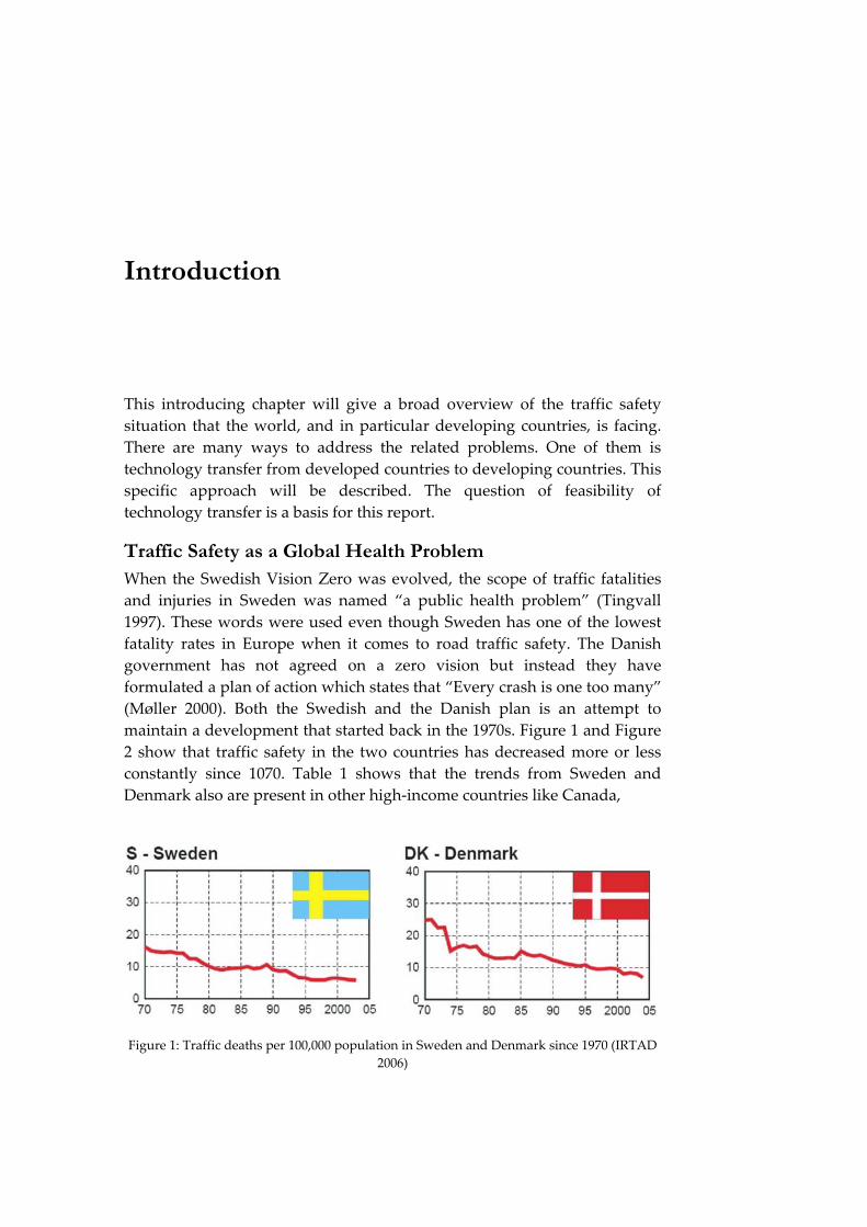
Traffic Safety as a Global Health Problem When the Swedish Vision Zero was evolved, the scope of traffic fatalities and injuries in Sweden was named “a public health problem” (Tingvall 1997). These words were used even though Sweden has one of the lowest fatality rates in Europe when it comes to road traffic safety. The Danish government has not agreed on a zero vision but instead they have formulated a plan of action which states that “Every crash is one too many” (Møller 2000). Both the Swedish and the Danish plan is an attempt to maintain a development that started back in the 1970s. Figure 1 and Figure 2 show that traffic safety in the two countries has decreased more or less constantly since 1070. Table 1 shows that the trends from Sweden and Denmark also are present in other high-income countries like Canada,
Figure 1: Traffic deaths per 100,000 population in Sweden and Denmark since 1970 (IRTAD 2006)

16 Traffic Calming in Delhi
Figure 2: Traffic deaths per 1 billion vehicle kilometres since 1970 (IRTAD 2006)
Finland, France, Italy and United States. In general the traffic safety has been increase in high-income countries since the 1960s and 1970s (Peden et al. 2004).
The situation is completely different when Sweden and Denmark – and other high-income countries – are compared with low- and middle-income countries. Table 2 gives the picture that only 10 % of the estimated global road traffic injury-related deaths appeared in high-income countries. These numbers are – both ethically and pragmatically – reasons for looking at traffic safety in a global perspective and not just national. When comparing the numbers in Table 1 the big difference in trends between high-income countries and low-income countries become very clear. Between 1975 and 1998 the fatality risk (deaths per 10,000 population) increased by more than 200 % in middle-income countries like Colombia and China. In a low-income country like Botswana the increase was above 300 %. As a contrast the high-income countries in Table 1 all have a decrease between 20 and 60 %. The described differences in fatality risk (fatalities per population, F/P) are explained by Koptis and Cropper (2005) as the product of vehicle ownership (vehicles per population, V/P) and fatalities per vehicles (F/V). In most low- and middle-income countries over the past 25 years, vehicle ownership grew more rapidly than fatalities per vehicles decreased. In high-income countries the development has been the opposite.
Table 3 compares the number of fatalities between 2000 and 2020 for six different regions of low- and middle-income countries. The predicted values are based on present policies and actions in road safety and do not consider additional road safety countermeasures. The table shows that the problem globally is increasing. The fatality number during the period will increase by more than 80 % in the low- and middle-income countries while the high-income countries will experience a decrease of more than 27 %. South Asia – which includes India – will experience a dramatic increase of more than 140 %. The world-total change between 2000 and 2020 is at 66 % and the fatality risk is increasing from 13 in 2000 to 17 in 2020. Thus traffic

Introduction 17
Table 1: Change in traffic fatality risk (deaths per 10,000 population) 1975-1998, a 1975-1997, b 1980-1998, c 1976-1998, (Kopits and Cropper 2005)
Country Change (%) 1975 - 1998
Canada −63.4 Hong Kong −61.7 Finland −59.8 Austria −59.1 Sweden −58.3 Belgium −43.8 France −42.6 Italya −36.7 Taiwan −32.0 United States −27.2 Japan −24.5 Malaysia 44.3 Indiab 79.3 Sri Lanka 84.5 Lesotho 192.8 Colombia 237.1 China 243.0 Botswanac 383.8
Table 2: Estimated global traffic injury-related deaths in 2002 (Peden et al. 2004)
Number Rate per 100,000 population
Proportion of total (%)
Low-income and middle-income countries
1,065,988 20.2 90
High-income countries 117,504 12.6 10 Total 1,183,492 19.0 100
Table 3 Predicted road traffic fatalities by region (in thousands), adjusted for underreporting, 1990-2020, a According to the regional classification of the World Bank (Kopits and Cropper 2005)
Regiona No. of countries
1990 2000 2010 2020 Change (%) 2000-2020
Fatality risk (deaths per
100,000 persons) 2000 2020 East Asia and Pacific 15 112 188 278 337 79.8 10.9 16.8 East Europe and Central Asia
9 30 32 36 38 18.2 19.0 21.2
Latin America and Caribbean
31 90 122 154 180 48.1 26.1 31.0
Middle East and North Africa
13 41 56 73 94 67.5 19.2 22.3
South Asia (includes India)
7 87 135 212 330 143.9 10.2 18.9
Sub-Saharan Africa 46 59 80 109 144 79.8 12.3 14.9 Sub-total 121 419 613 862 1,124 83.3 13.3 19.0 High-income countries 35 123 110 95 80 -27.8 11.8 7.8 World-total 156 542 723 957 1,204 66.4 13.0 17.4

18 Traffic Calming in Delhi
safety is not just a public health problem in Sweden but must be understood as a global health problem.
Table 1 and Table 3 refer to the World Bank’s Traffic Fatality and Economic Growth (TFEG) project (Kopits and Cropper 2005). However, another model also gives a prediction for the future trends in road traffic fatalities: the WHO Global Burden of Disease (GBD) project (Murray and Lopez 1996). The main difference between the two model’s data is that TFEG is using transport, population and economic data while GBD is using health data. The results of the GBD project are mostly given in DALYs – Disability Adjusted Life Years. DALYs is an adjusted number of YLL – Years of Life Lost – where it is taken into consideration that a traffic crash victim might survive a crash but live with a disability. DALYi is the sum of YLLi and YLDi, where i is a given condition – e.g. traffic crash – and YLD is years lived with a disability. According to the GBD project road traffic injuries will become the third leading cause of DALYs lost, see Table 4. Thus, the overall message is the same as for the TFEG project: if low- and middle-income countries follow historic trends a large escalation in global road traffic mortality over the next decades is expectable. However, the two models differ on the global road traffic deaths for 2020. The TFEG project states that the number will climb to over 1.2 million by 2020 while the GBD project states that road traffic crashes will climb to the sixth highest position with 2.4 million by 2020. Kopits and Cropper (2005) discuss the difference and explain it by the fact that the GBD project starts at a higher base of deaths by 1990. (Kopits and Cropper 2005; Murray and Lopez 1996)
Despite differences between the two models there is a clear message behind both of them: helping low- and middle-income countries tackle the problem of road traffic crashes must be a priority. The argument for this is very simple: road traffic crashes is no longer a national problem but a global health problem where the situation in low- and middle-income countries effects the global predictions for the next decades.
Table 4: Change in rank order of DALYs, world, 1990-2020 (Murray and Lopez 1996)
1990 2020 Rank Disease or injury Rank Disease or injury 1 Lower respiratory infections 1 Ischaemic heart disease 2 Diarrhoeal diseases 2 Unipolar major depression 3 Perinatal conditions 3 Road traffic injuries 4 Unipolar major depression 4 Cerebrovascular disease 5 Ischaemic heart disease 5 Chronic obstructive pulmonary dis. 6 Cerebrovascular disease 6 Lower respiratory infections 7 Turberculosis 7 Turberculosis 8 Measles 8 War 9 Road traffic injuries 9 Diarrhoeal diseases 10 Congenital abnormalities 10 HIV

Introduction 19
Traffic Safety in Less Motorized Countries It took decades – over the last 50 years – while the now highly motorized countries were getting motorized before right strategies and measures were evolved. Not until the 1960s and 1970s the trends of road traffic crashes started to go downwards. The logical question is whether countries that right now are undergoing a motorization process can avoid a long period struggling to find the right strategies and measures. Can the lesson learned from the highly motorized countries be used in the low motorized countries? This question has been tried answered by establishing links between road traffic crashes, growth in motorization and economic growth.
The empirical lesson from high income countries is that growth in mobility not necessarily will lead to higher rates of fatalities. Two models using data from respectively 1938 and 1968 tried to illuminate a relationship. Both models came to the conclusion that fatalities per motor vehicle will decrease as motor vehicles per head of population increases. The two models, however, are not without weaknesses (Peden et al. 2004). Other studies try to establish a link between fatality risk and economic development. The findings from three studies are showed in Figure 3, Figure 4 and Figure 5. They all show the same general tendency when fatalities per population is plotted against income (Mohan 2004; Söderlund and Zwi 1995; Kopits and Cropper 2005). As income grow, fatality risk will increase until a certain peak level and then decline. On all three figures an invented u-shaped pattern is clear which illustrates this tendency. Kopits and Cropper (2005) found that fatality per population increases sharply until the gross domestic product reaches a peak between $6100 and $8600 (1985 international dollar values). After this peak motorization will slow down and investments in traffic safety are more likely, which will cause a decrease in fatality per population. The results all show a clear link between economic development and increased exposure to risk – which follows from mobility and motorization. (Peden et al. 2004)
To make road traffic crashes start to take a downward trend it is not enough to sit back and wait for a country to reach a certain point of motorization or gross domestic product. Policy makers and engineers in each country will have to work focused at finding national adapted strategies and measures. However, the responsibility is not only a national matter. The World Bank – and high-income countries through developing aid – is financing road infrastructure projects in low- and middle-income countries. If these projects lack the focus on traffic safety, then the positive effect will be negligible. This is due to economic reasons. The national

20 Traffic Calming in Delhi
Figure 3: Fatalities per million population for different countries vs. income (Mohan 2004)
Figure 4: Fatalities per 100,000 population vs. income (Söderlund and Zwi 1995)
Figure 5: Fatalities per 10,000 population vs. income (Kopits and Cropper 2005)

Introduction 21
expenses from road traffic crashes in low- and middle-income countries surpass the amount of money given in development aid from high-income countries. World Bank projects without focus on traffic safety will so to speak keep up an unsustainable global economic development. (Peden et al. 2004; Ross et al. 1994)
An additional reason for giving priority to traffic safety in developing countries is a moral reason. Road traffic crashes do not necessarily have to be the price to pay for mobility and economical development. This must be the way of addressing the present problems. This, however, demands a change in the way of thinking by the public. For instance it must be understood that injuries are preventable and injuries happen because of crashes, not because of accidents. Beside this there is a need for more visionary thinking – e.g. zero visions. (Peden et al. 2004; Mohan 2004)
Technology transfer There are many ways of addressing the problem of road traffic fatalities in low- and middle-income countries. One of them is technology transfer of physical measures from high-income countries. Other ways are institutional reinforcements, law enforcements, education, system approach policies, etc. Technology – or knowledge – transfer is by no mean a miracle drug without pitfalls. Despite good intensions the expected results might fail to come. The next paragraphs will try to clarify some of the difficulties combined with technology transfer.
The traffic structure in India and many other low- and middle-income countries – not only in South Asia - are completely different compared to most high-income countries. This means that the strategies and lessons learned not directly can be transferred from their origins. Research has to be made before the right methods and measures are found. In low- and middle-income countries the most common transport modes are walking, cycling, motorcycling and public transport. In contrast, the predominantly traffic mode in high-income countries are private cars, see Table 5. The mixed traffic in low- and middle-income countries carry a wide range of users, which includes pedestrians, human drawn carts, animal drawn carts, bicyclists, motorcyclists, three-wheeled motor vehicles and four-wheeled
Table 5: The contrast of car ownership in respectively low- and middle-income countries and high-income countries (Peden et al. 2004)
Country/region People per car North America 2-3 Europe 2-3 India 220 China 280

22 Traffic Calming in Delhi
motor vehicles. All these road user groups often share the same road space without separation. The traffic composition also reflects the distribution of killed in various modes of transport, see Table 6. From this table it becomes clear, that vulnerable road users – like pedestrians and two-wheelers – experience a much higher exposure in e.g. India than in USA. This high exposure is mainly explained by the high proportion of motorcycles and scooters in the road spaces. (Mohan and Tiwari 1998; Peden et al. 2004)
Even though car ownership in the low- and middle-income countries is predicted to increase, then the proportion compared with e.g. motorcycles will still be low in the next 20-30 years (Peden et al. 2004). Because of this it is important not to think of road user patterns from high-income countries as the norm for all situations. Neither must it be seen as a need to mimic the conditions in high-income countries in order to obtain positive results in low- and middle-income countries. Instead schemes must be promoted within the existing conditions. These include low per-capita incomes, presence of mixed traffic, low capacity for capital intensive infrastructure, and different law enforcement capabilities. (Mohan and Tiwari 1998)
International experts and professionals from high-income countries often will get the initial thought that the current traffic safety situation is due to poor driver behaviour and bad education. These thoughts, however, do not have to be right. Studies from the Philippines and India have indicated that road users seem to optimise throughput through intersections by non-observance of formal rules. This optimisation process may look chaotic or complex. These circumstances just makes it even more important to keep focus at the existing conditions as the environment for schemes to be implemented in – not environments and conditions as in high-income
Table 6: Road users killed in various modes of transport, as a % of all fatalities, MTW: Motorised Two-Wheeler. (Mohan and Tiwari 1998)
City, Nation (year) Pedestrians Bicyclists MTWs Motorized four-
wheelers
Others
Delhi, India (1994) 42 14 27 12 5 Thailand (1987) 47 6 36 12 - Bandung, Indonesia (1990)
33 7 42 15 3
Colombo, Sri Lanka (1991)
38 8 34 14 6
Malaysia (1994) 15 6 57 19 3 Japan (1992) 27 10 20 42 1 The Netherlands (1990)
10 22 12 55 -
Norway (1990) 16 5 12 64 3 Australia (1990) 18 4 11 65 2 USA (1995) 13 2 5 79 1

Introduction 23
countries. This is exactly the challenge of technology transfer: through research to adapt already known schemes and measures – developed for high-income countries – to the situation of the existing traffic safety problems of low- and middle-income countries. (Mohan and Tiwari 1998)

24 Traffic Calming in Delhi

Chapter 1
Aim and Formulation of Hypotheses
This chapter gives an introduction to traffic calming as a measure to increase traffic safety. Further the current Indian traffic safety situation will be described. From this the main problem and two hypotheses will be set. The hypotheses will be the basis of the report. The chapter ends with a description of this report’s strategy and delimitations.
1.1 Previous Results with Traffic Calming Traffic calming is sometime confused with the different concept of speed management. To prevent confusion in this report the two concepts will be defined:
⎯ Speed management is about regulating the speed (passability) of cars through legislation, marking, visual or physical effects.
⎯ Traffic calming is about reducing the passability or accessibility of cars through legislation, marking, visual or physical effects. (Kjemtrup and Herrstedt 1992)
This report will only deal with the latter – traffic calming – and it will take a basis in the experiences and conclusions already agreed on – mainly in Sweden and Denmark. This section will begin with a brief introduction to the history of traffic calming in Europe. After that, different examples of the use of traffic calming and studies about traffic calming from Norway, Sweden and Denmark will be introduced.
1.1.1 Traffic Calming in Europe During the 1950s and the 1960s the car ownership increased heavily in Europe. This caused increasing traffic intensity on both arterial roads and local roads resulting in an increase of crashes, particularly between motor vehicles and vulnerable road users. The main thought was that separation of the road users could solve the new situation. A separation of slow-moving light road users from fast-moving heavy road users would remove the risk of conflicts, it was thought. This was internationally recognized and implemented throughout Europe when new traffic systems arose. In

26 Traffic Calming in Delhi
many existing traffic systems it was not possible to implement the concept of separation because of too little space. As a result from this, different strategies were evolved during the 1960s and the 1970s. In Sweden the SCAFT guidelines were introduced during the 1960s. These guidelines suggested a classification of the road network where the lowest classes could have speed limits lower than 50 km/h. The SCAFT guidelines build on the principles of separation. In the Netherlands the “Woonerf design” was introduced, containing the first traffic calming initiatives. The Woonerf design integrated the different road users and used physical measures for speed reduction. In the late 1970s the Woonerf design was implemented in Denmark. Here the design of physical speed reducing measures and integration of road users became known as “Section 40 areas” or “shared areas”. In the 1980s and 1990s the concepts of narrowing roads and establishing of physical obstacles to slow down the speed continued to have great interest. The ideas also now were used on arterial roads in Norway and Denmark. This was called Environmentally Adapted Through Roads. While many European countries worked with traffic calming – often inspired by the Woonerf design – on local roads it was mostly France, Germany and Denmark that also implemented the concepts onto arterial roads. (Kjemtrup and Herrstedt 1992)
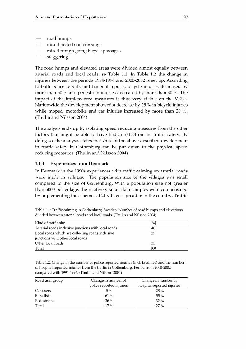
1.1.2 Traffic Calming in Gothenburg During the 1990s a great effort was made in the Swedish town Gothenburg to increase traffic safety. The population of Gothenburg is nearly 500,000 (in 2005) and the city is located at the west coast of Sweden. The strategy used was with physical measures to lower the speed of motor vehicles in areas and around traffic sites, where pedestrians and bicyclists where present, and with different measures to reduce/separate the car traffic from the vulnerable road users at the same sites. An analysis of the scheme that was carried out was made in 2004. Here comparison is made between the years 1994-1996 and 2000-2002. The reason for this is that a great decrease in injuries happened in the end of the 1990s. Besides, great investments in traffic safety measures were made in that period too. For instance 80 % of the more than 700 humps were constructed between 1996 and 2000. Gothenburg naturally changed in many other ways during the 1990s – demography, growth in road user groups, use of bicycle helmet, use of seat belt, etc. ´The analysis concludes that the change with the biggest impact on traffic safety where the physical speed reducing measures. When the analysis was made 1840 traffic sites in Gothenburg were fitted out with a total of 2064 physical speed reducing objects. Of these 2064 objects, 89 were roundabouts and 1781 were elevations of some kind of a form. Some of the most used measures were:
Aim and Formulation of Hypotheses 27
⎯ road humps ⎯ raised pedestrian crossings ⎯ raised trough going bicycle passages ⎯ staggering
The road humps and elevated areas were divided almost equally between arterial roads and local roads, se Table 1.1. In Table 1.2 the change in injuries between the periods 1994-1996 and 2000-2002 is set up. According to both police reports and hospital reports, bicycle injuries decreased by more than 50 % and pedestrian injuries decreased by more than 30 %. The impact of the implemented measures is thus very visible on the VRUs. Nationwide the development showed a decrease by 25 % in bicycle injuries while moped, motorbike and car injuries increased by more than 20 %. (Thulin and Nilsson 2004)
The analysis ends up by isolating speed reducing measures from the other factors that might be able to have had an effect on the traffic safety. By doing so, the analysis states that 75 % of the above described development in traffic safety in Gothenburg can be put down to the physical speed reducing measures. (Thulin and Nilsson 2004)
1.1.3 Experiences from Denmark In Denmark in the 1990s experiences with traffic calming on arterial roads were made in villages. The population size of the villages was small compared to the size of Gothenburg. With a population size not greater than 5000 per village, the relatively small data samples were compensated by implementing the schemes at 21 villages spread over the country. Traffic
Table 1.1: Traffic calming in Gothenburg, Sweden. Number of road humps and elevations divided between arterial roads and local roads. (Thulin and Nilsson 2004)
Kind of traffic site [%] Arterial roads inclusive junctions with local roads 40 Local roads which are collecting roads inclusive junctions with other local roads
25
Other local roads 35 Total 100
Table 1.2: Change in the number of police reported injuries (incl. fatalities) and the number of hospital reported injuries from the traffic in Gothenburg. Period from 2000-2002 compared with 1994-1996. (Thulin and Nilsson 2004)
Road user group Change in number of police reported injuries
Change in number of hospital reported injuries
Car users -5 % -28 % Bicyclists -61 % -55 % Pedestrians -36 % -32 % Total -17 % -27 %

28 Traffic Calming in Delhi
calming was not the only aim with the project, which had the common title of Environmentally Adapted Through Roads. Focus was also pointed at visual satisfying design, a fit to the local village- and traffic environment and reducing the barrier effect of roads. The focus, however, was delimitated to the main arterial through traffic road in each village. The measures used were a mix of different physical speed reducing measures. The most common were:
⎯ Roundabouts / mini roundabouts ⎯ Middle islands ⎯ Side islands ⎯ Islands where running over is possible ⎯ Islands with plantation ⎯ Elevated areas
The early experiences with environmentally adapted through roads in Denmark were made in the 1980s at three so called pilot villages. The experiences from the 1990s’ projects are analysed in a report made by the Danish road directorate in 2003. (Wellis et al. 2003)
The report analyses the effect of the implemented schemes by comparing police reported crashes from 5 year periods before and after the implementation corrected with control groups. Some of the results from the report are showed in Table 1.3. The table sums up the results from all the 21 villages. It shows that all types of crashes have been reduces by 20 % while crashes with person injury have been reduced by 29 %. Crashes with property damage have been reduced by 10 %. By speed measurements at 11 of the 21 villages it was found that the mean value was decreased after the implementation by 16 %, see Table 1.4. Even more interesting it was found – by making new measurements in 2003 – that the decrease was maintained circa 7 years after the implementation. The found effects seem to be the result of a combination of the physical speed reducing measures used.
Table 1.3: Traffic calming in Denmark. Crash data from before implementation, after and the expected number for all the 21 villages. (Wellis et al. 2003)
Arterial roads with high amount of through traffic
Reduction
Before After Expected without project
(numbers) ( % )
All crashes 144 87 108.1 21.1 20 % Person inj. crashes 65 33 46.6 13.6 29 % Only property damage crashes
79 54 59.8 5.8 10 %
Fatalities + severe injuries
52 18 29.5 11.5 39 %
All person injuries 93 47 66.5 19.5 29 %

Aim and Formulation of Hypotheses 29
Table 1.4: Traffic calming in Denmark. Mean value of the average speed at selected sections at 11 of the 21 arterial roads. (Wellis et al. 2003)
Mean value Before (1994-1995) 58 km/h After (1995-1996) 50 km/h After (2003) 48 km/h
1.1.4 Studies about Traffic Calming Both examples from respectively Gothenburg and Denmark show positive results from implementing traffic calming measures. However, to make clear that the achieved effects are not just Scandinavian phenomena a third study is introduced. During the last 30 years, area-wide traffic calming schemes have been implemented in many motorized countries. Elvik (2001) made a meta-analysis – an analysis of existing analyses – based on 33 studies – most of them from Europe. All studies were non-experimental before-and-after studies containing results defined in terms of the number of accidents. Some of the common characteristics for the studies were:
⎯ The area in which traffic calming was introduced was a predominantly residential area, often located close to the central business district of a major city.
⎯ Area wide traffic calming involved a reclassification of the street network in the area, aiming to remove through traffic from residential streets and concentrate it on a few streets designated as main roads.
⎯ The most often speed reducing measure used in local roads was humps. (Elvik 2001)
The results from the meta-analysis are remarkably consistent both across different levels of accident severity and across modes of analysis. From Table 1.5 it becomes clear that the biggest effect of area-wide traffic calming schemes should be expected at local roads. Here a 25-55 % reduction was found from the meta-analysis. In the whole area the reduction was found to be between 15 and 20 % while arterial roads were found to have a reduction between 8 and 15 %.
Table 1.5: Results of the meta-analysis of 33 existing studies of area-wide traffic calming schemes – mainly in Europe. (Elvik 2001)
Type of road Reduction in the number of accidents Whole area 15-20 % Arterial roads 8-15 % Local roads 25-55 %

30 Traffic Calming in Delhi
On the basis of the results, it is concluded about traffic calming – consisting of measures designed to discourage non-local traffic from using residential streets and reducing the remaining traffic – that the existing evaluation studies are stable over time and of similar magnitude in eight countries. Besides it is concluded that it is unlikely that ”confounding factors not controlled in evaluation studies alone could produce as stable effects as they would have to account entirely for the findings of the evaluation studies. It seems more likely that the results of at least the best-controlled studies mostly reflect the effects of traffic calming”. (Elvik 2001)
1.2 Traffic Safety in India Today As described through the previous sections of this chapter, traffic calming has been used during the last 30 years with positive results in many motorized / high-income countries. To understand the premises for using traffic calming in India, an introduction to the traffic situation in India today will follow in this section. Because the field studies took place in Delhi, most of this section will be about this metropolis. Delhi is the sixth most populous metropolis in the world with a population above 15 million.
The traffic composition in Delhi is a mix of heterogeneous traffic. Roughly it consists of eight groups: pedestrians, bicyclists, human- and animal drawn carts, motorbikes, Three-wheeled Scooter Rickshaws (TSR), cars, trucks and busses. TSRs are local made taxis with three wheels and a scooter engine, see Figure 1.1.
Figure 1.1: TSRs (Three-wheeled Scooter Rickshaws) are a cheap and easy way of transportation in Delhi

Aim and Formulation of Hypotheses 31
All road users more or less share the same area. No separation is made between bicycles and motor vehicles, and though pavements are widespread their bad condition often results in pedestrians using the carriageway. Also markets with stalls can take up the width of the pavement. Thus slow moving, unprotected road users such as pedestrians are mixed with fast moving, heavy vehicles such as trucks and busses. Combined with limited enforcement of speed limits the situation can become crucial in the case of a crash. (Tiwari et al. 1998)
Motorbikes constitute a huge proportion of the traffic in Delhi. Table 1.6 shows that about 60 % of the motor vehicles in Delhi consist of motorbikes and scooters. Such high proportions are not seen in European or high-income countries where cars traditionally have been dominating the road traffic. The number of four-wheeled motor vehicles in India has increased by 23 % between 1990 and 1993. However, most of the increase in the national vehicle fleet is expected to be in motorized two-wheelers. The big proportion of motorbikes is also reflected in the injury statistics. A study in New Delhi found that 16 % of injured pedestrians had been struck by motorized two-wheelers. (Peden et al 2004)
With a mix of up to eight different road user groups, where motorbikes is a big group, the traffic can be defined as heterogeneous. This is characterised by lack of any effective channelization, mode segregation or speed control. In this situation flow patterns result in a natural optimisation of road use due to self-organisation by road users. The lane discipline in heterogeneous traffic is much different than in homogeneous traffic, which is showed on Figure 1.2. On this figure it showed how narrow vehicles fill-in the lateral and longitudinal gaps between wide vehicles. Especially for foreigners and people not used to this kind of traffic it might look like “chaos” moving towards a gridlock. The thought of “chaos” may also be caused by non-observance of formal traffic rules. Non-observance is not necessarily due to lack of awareness of the meaning of rules, signs or making, but due to the priority which is given to the informal rules by road users. Lane discipline and non-observance of formal rules can be explained as a kind of an optimization process. This is mainly because heterogeneous traffic uses on-street space more efficiently than homogeneous traffic. (Tiwari et al. 2005)
Table 1.6: Motor vehicles registered in Delhi in 2004. MTW: Motorised Two-Wheeler, TSR: Three-wheeled Scooter Rickshaw. (Delhi Traffic Police 2004)
Priv. cars MTWs Taxis TSRs Trucks Busses Total 1,415,729 2,811,951 22,239 129,862 160,852 41,866 4,582,499
31 % 61 % 1 % 3 % 4 % 1 % 101 %

32 Traffic Calming in Delhi
Figure 1.2: Homogeneous traffic has one-dimensional queues while heterogeneous traffic has two-dimensional queues (above). Homogeneous traffic has lane discipline while
heterogeneous traffic has parallel entity-following (below).
In urban areas in whole Denmark there is an equal distribution between crashes at road junctions and on road stretches (Transport- og Energiministeriet 2006). In India the situation is another. In Delhi only 18 % of the pedestrian fatalities occurred at junctions and 82 % occurred on road stretches (1985 figures). Of all bicycle fatalities in Delhi 73 % happened on road stretches (2002 figures). Generally for all crash types the majority occurs mid-block (between intersections) on divided (with middle separation) road stretches. (Mohan and Bawa 1985; Tiwari et al. 1998; Mohan 2002)
The overall statistics for bicycle fatalities in Delhi show that 60% of bicycle fatalities occur outside the peak hour when traffic volumes are lower but motor vehicle speeds are high. Bicycle fatalities are very prominent between 6 am to 10 am while motorized two-wheelers are prominent between 8 am and 10 am. This distribution is caused by the fact that many poor, who do not own a motorized vehicle, often live in the outskirts of Delhi and will have to use more time on transportation on the road. (Mohan and Bawa 1985; Mohan 2002)

Aim and Formulation of Hypotheses 33
India as a whole had a fatality rate of 80 fatalities per million persons while Delhi had a fatality rate of 143 per million persons, the second highest among India’s metropolis (2004 figures). Non-motorized road users accounted for 60-80 % of all the fatalities in 2004. Motorized two-wheelers comprise approximately 60 % of all motorized vehicles and constitute 30 % of fatalities. Whereas heavy vehicles like trucks and busses are associated with 50-70 % of all road crashes. Table 1.7 shows that 55 % of all pedestrian fatalities were struck down by busses (33 %) or trucks (22 %). 69 % of all bicycle fatalities were struck down by busses (31 %) or trucks (38 %). (Delhi Traffic Police 2004)
Table 1.8 shows that busses and trucks are involved in 73 % of all fatal crashes in Delhi. However, the majority of victims are not from this road user group. Around 80 % of killed road users in Delhi in 2004 were part of the unprotected road user group. Table 1.9 shows that 84 % were VRUs (Vulnerable Road Users). Figure 1.3 shows how VRUs are exposed, here on a MTW. The combination of high crash involvement among VRUs and the majority of crashes happening at mid-block is completely different from experiences in high-income countries, which traditionally aim at reducing crashes between motorized four-wheelers equally distributed between junctions and straight roads. (Mohan and Tiwari 1998).
Table 1.7: Road traffic crash characteristics in Delhi in 1994, a: Motorized Two-Wheelers, b: Three-wheeled Scooter Rickshaw. (Tiwari et al. 1998)
Registered vehicles [%]
Road users Pedestrian fatalities
struck by road users [%]
Bicyclists fatalities
struck by road users [%]
Fatality distribution of all road users
[%] - Pedestrians 0.0 0.0 42.0 - Bicyclists 0.0 3.0 14.0 67.0 MTWa 9.0 8.0 27.0 3.4 TSRb 5.0 3.0 3.0 23.3 Cars / taxi 20.0 14.0 5.0 1.1 Busses 33.0 31.0 5.0 5.1 Trucks 22.0 38.0 2.0 0.1 Others 11.0 3.0 2.0
Table 1.8: Proportion of motor vehicles involved in fatal crashes in Delhi (Mohan 2004)
Vehicles involves, per cent Trucks Busses Cars TSR MTW Total
40 33 16 4 7 100
Table 1.9: Road traffic victims killed in Delhi in 2004 (Delhi Traffic Police 2004)
Pedestrians Bicyclists MTW Car Other Total 900 178 467 40 247 1832
49 % 10 % 25 % 2 % 13 % 99 %

34 Traffic Calming in Delhi
Figure 1.3: A typical picture of a whole family on a scooter (MTW) in the mixed traffic of Delhi.
Table 1.8 also show that TSRs (Three-wheeled Scooter Rickshaws) are involved in only 4 % of the fatal crashes in Delhi. Table 1.8 shows the same picture; that TSRs are involved in few – respectively 5 % and 3 % - pedestrian and bicyclist fatalities. In addition, the table shows that TSR-road users constitute a small percentage of the traffic fatalities. Fatalities among TSR-road users (3 %) are smaller than e.g. cars (5 %) and busses (5 %). Thus TSRs represent a relatively safe way of transportation in Delhi.
According to the Delhi Traffic Police 9083 crashes were recorded in 2004 in Delhi. Of these crashes 1832 persons lost their lives. The national trend for road traffic fatalities has been rising steadily since the 1970s, which Figure 1.4 shows. The future does not look much brighter if the ongoing trends and strategies continue. Then the road death rate in India will not begin to decline until 2042. (Delhi Traffic Police 2004; Kopits and Cropper 2005)
Mohan (2004) argues that new strategies must be developed, involving:
⎯ Institutional reform ⎯ New systems for data collection and analysis ⎯ Safer road measures (e.g. traffic calming) ⎯ Safer vehicle measures (e.g. new front design of busses and trucks) ⎯ Legal measures and enforcement (e.g. speed limits) ⎯ Community support
Strategies must include both short term (1-3 years) and long term (4-10 years) goals. Priorities must be identified in an Indian context based on present available data. As more detailed data will become available in the future the priorities must be modified correspondingly. (Mohan 2004)

Aim and Formulation of Hypotheses 35
Figure 1.4: Road traffic fatality trend in India (Peden et al. 2004)
1.3 Formulation of Problem The overall goal of this report is to examine with which measures traffic calming can be used to increase the level of traffic safety in Delhi. Traffic calming is a well known and widespread method in many highly motorized countries. In India the method is expected to have a huge potential (Mohan 2004). Thus, the basic hypothesis is:
Traffic calming, as a measure to increase traffic safety can, with minor adaptations, be used in its present form in an Indian urban environment.
To understand the feasibility of transferring measures from highly motorized countries to less motorized countries it is necessary to look at behaviour at different road users on a micro level. This will result in that analyses are made with respect to single conflicts between two (possibly more) road users. These conflicts on a micro level will be analysed with the theory from the Swedish traffic conflict and thus be given a general perspective. Traffic conflict technique is an observation and analysis technique that not is dependent on reliable crash data. This is important when working in a low- and middle-income country where it can be difficult to get access to crash data, possibly because they do not exist.
Problems affiliated to transferring measures are related to the differences between countries. In this report three issues will be held at focus:
⎯ The physical layout of the environment

36 Traffic Calming in Delhi
⎯ The behaviour of the road users ⎯ The willingness of the road users to take risks.
The last of these represents the differences in how road users are willing to accept risky traffic situations. These three issues will in this report be used as a basis to give an answer to the main problem:
How can a prognosis look like that concerns the feasibility of using traffic calming, with minor adaptations with respect to its present form – as it is described in the Danish design rules – as a measure to increase traffic safety in Delhi?
To answer the main problem, two hypotheses are formulated:
Hypothesis 1: The Swedish traffic conflict technique is built on universal assumptions. Thus, the method can be used in the mixed traffic composition of Delhi to give diagnoses to problems at traffic sites. For conflict studies to give useable results, the distinguishing between serious and non-serious conflicts has to be fitted to the local conditions in Delhi with respect to differences in physical design, road user behaviour and willingness of risk. The borderline between serious and non-serious conflicts are located at a “higher” position similarly as the willingness of risk is located at a “higher” position when India is compared with Sweden.
Hypothesis 2: The existing facilities for pedestrians – crossing paths, footpaths, etc. – in the urban areas are inadequate with respect to the pedestrian’s needs (Quimby et al. 2003). Unless there are built-in measures to slow down the speed of the traffic, pedestrian crossings can function as death traps (Mohan and Bawa 1985). The severity of conflicts involving crossing pedestrians and motor vehicles are closely related to the speed of the motor vehicles and the hierarchy in the traffic. Thus the traffic safety can be increased by using the Danish design rules for traffic calming.
1.4 Strategy Field studies, with gathering of data at traffic sites in Delhi, are the main strategy. The field studies are designed to give answers to the hypotheses. Through the work with the hypotheses and the field studies, different measures are being mentioned. These measures will be presented in a prognosis. The prognosis shall clarify which measures which are usable for increasing traffic safety in Delhi. At the same time this will be the answer to the main problem formulated above.
1.5 Delimitations Only three issues concerning the differences between India and the Nordic countries are included. This is, as described in the problem formulation, the physical layout of the environment, the behaviour of the road users, and the willingness of the road users to take risks. The three issues are believed

Aim and Formulation of Hypotheses 37
to be sufficient in order to produce relevant conclusions regarding the feasibility of using traffic calming in India.
The data collection will be done by the author. No funds have been collected for the aim of hiring a local team to help with the data collection. This will result in relatively small data samples.

38 Traffic Calming in Delhi

Chapter 2
Hypothesis Testing
This chapter will explain how the hypotheses will lead to the field studies and further to the data material that will be the basis for the analysis, which will follow in the next chapter.
2.1 How to Test the Hypotheses In the previous chapter two hypotheses were introduced. In this section the hypotheses will be further explained and the connection to the field studies will be clarified.
2.1.1 Hypothesis 1 The first hypothesis will be examined by doing traffic conflict technique studies at traffic sites in Delhi. It is the aim to determine the threshold between serious and non-serious conflicts in an Indian environment. This will be done by using a subjective severity scale in comparison with the original distinguishing between the severity levels. Overall, the field studies related to this hypothesis is expected to give useful knowledge about the use of the Swedish traffic conflict technique in an Indian environment.
Hypothesis 1 is necessary because this report’s field studies mainly are based upon the traffic conflict technique. In this case it is decisive to know how practicable this analysis technique is when working in the mixed traffic compositions of Delhi.
2.1.2 Hypothesis 2 The second hypothesis will be examined by doing traffic conflict studies at a mid-block traffic site with a mix of pedestrians – or VRUs – and motorized vehicles. The conflict data will be followed by speed measurements and general studies of the road user behaviour. The hypothesis will provide the basis for the work on suggestions for the use of traffic calming measures in Delhi.

40 Traffic Calming in Delhi
2.2 Selection of Traffic Sites in Delhi After the arrival to Delhi the search for suitable traffic sites for the field studies began. A minimum of two sites were needed to examine the two hypotheses. The search was assisted by the staff at TRIPP (Transportation Research and Injury Prevention Programme at IIT). The traffic sites were intended to have an “interesting” traffic composition, existing of all kind of road user groups – specially a mix of VRUs and motor vehicles. Taken into account that police reports of crashes not were available, the traffic sites did not need to be black spots or similar accident prone sites. Two traffic sites were selected between five possible sites. Those two will be introduced in the following section. They are named Orthonova and Dilli Haat.
2.3 Introduction to Selected Sites Delhi is a metropolis with a population of 15 million covering an area of more than 1000 sq kms including the suburbs. This report will not give an introduction to whole Delhi’s traffic network or land use. Instead focus will be at the two selected traffic sites. They are both located in the southern part of Delhi, see Figure 2.1 and Figure 2.2. Orthonova is located south of the Outer Ring Road. Dilli Haat is located just south of Safdarjang Airport and north of the (inner) Ring Road.
Figure 2.1: Road network of Delhi. Outer Ring Road, Ring Road and Safdarjang Airport are good orientation marks. The blue rectangle refers to Figure 2.2. (Maps of India 2006)

Hypothesis Testing 41
2.3.1 Orthonova The traffic junction, which in this report is called Orthonova, is a four-armed signalized intersection. It services all kind of road user groups that is present in Delhi. The intersection is located at Lal Bahadur Shastri Marg or Dr B R Ambedkar Marg according to different maps. “Marg” is Indian for “road” and in the following the road will be named as Shastri Marg. The easiest way to describe the location is the south-east corner of Pushpa Vihar, Sector 7, see Figure 2.3. Pushpa Vihar is mainly a residential area but with schools, markets and an enormous, new shopping centre, which is being built on now. On the east side of Shastri Marg, a green area is located – Jahanpanah City Forest – together with a residential area – Dakshinpuri. Shastri Marg is a part of a planned high capacity bus system (HCBS) that will connect the southern part of Delhi – Mahrauli Badarpur Road south of Orthonova, see Figure 2.2 – with the central part of Delhi – Delhi Gate and
Figure 2.2: Sectional view of Figure 2.1. Orthonova is located in the lower right between Outer Ring Road and Mehrauli Badarpur Road. Dilli Haat is located in the upper right
between Safdarjang Airfield and Ring Road. (Eicher 2006)

42 Traffic Calming in Delhi
possibly Kashmiri Gate, not illustrated. TRIPP has been involved in the planning process and has made a suggestion for redesign of the whole stretch. These plans will be commented on later in this report.
Figure 2.3 shows the surrounding areas of the intersection. At the upper right corner office buildings are located and behind them the Jahanpanah City Forest. The office buildings do not generate much traffic – neither light nor heavy. At the lower right corner office buildings are also located. These offices generate some car traffic. East of the offices Dashkinpuri residential area is located. This area is a lower medium-class area which generates a lot of bicycle traffic. At the lower left corner a school is located. This generates a lot of car traffic around morning and early afternoon, when school children are sent to and fetched from school. At the upper left corner a residential area is located. This area does not have direct connection to the intersection and thus it does not generate much traffic – neither light nor heavy.
Figure 2.3: The traffic junction Orthonova looks like two staggered T-junctions on the map. In reality the junction is a four armed signalized junction. (Eicher 2006)

Hypothesis Testing 43
Figure 2.4 shows that the intersection actually is a four-armed junction and not two staggered T-junctions. The main road – Shastri Marg – has physically separated lanes which also is the situation at the intersection’s eastern leg. Shastri Marg has two car lanes and one bus lane marked with white painting. In addition Shastri Marg has service lanes south of the intersection in the southward direction and north of the intersection in both directions. Service lanes are secondary lanes parallel with the main road. Only the single service lane south of the intersection is available for driving and parking. The two others are taken up by hawkers and their stalls. At the time when field studies were made the following stalls were observed (the numbers refer to Figure 2.4): (1) bicycle repairing, (2) empty stall, (3) tobacco, water, sweets, etc., (4) as 3, (5) as 3, (6) as 3, (7) street food, (8) phone connections, (9) juice shop, (10) tobacco, (11) juice shop, (12) barber, (13) motorbike helmets and (14) flowers.
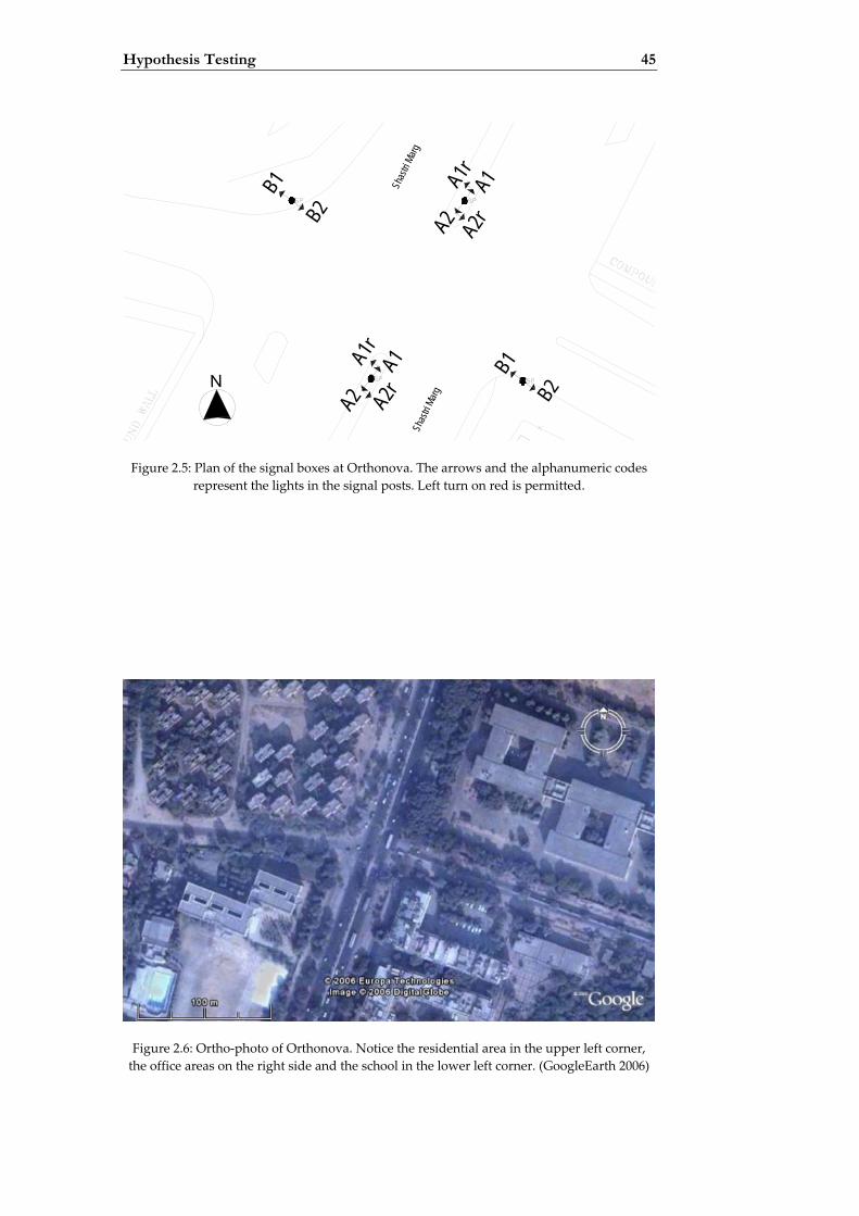
The intersection is signalized and the cycle length is divided into five phases. Left turn on red is allowed. During observations at the intersection the phases were checked manually for the peak hours. It was not possible to find agreement between the observed phases and the informed phases, which was provided by Delhi Traffic Police through TRIPP. The cycle length was observed to be 140 sec. while it was informed to be 130 sec., both for the peak hours. The division into phases agreed but not the phase times. Both the observed and the informed cycle are showed in Appendix A. Table 2.1 and Figure 2.5 show the division into phases.
N
Orthonova Junction
1 2
34
56
8
910
11
121314
Shas
tri Ma
rg
Shas
tri Ma
rg
Figure 2.4: Technical base plan of Orthonova intersection. The numbers in circles refers to stalls explained in the text.

44 Traffic Calming in Delhi
Traffic counts were provided by Delhi Traffic Police through TRIPP. Counts for the morning peak hour and the evening peak hour are showed in Appendix D. Table 2.2 shows numbers from the morning peak hour between 9 and 10 am. It is worth noticing that the total numbers of cars, motorized two-wheelers and bicycles almost are equal. Also it is worth noticing that the number of bicycles coming from south is very high. The equivalent number of private car units is showed in the table’s last column. From this column it is possible to get en idea of the AADT of the roads. When it is assumed that the peak hour equals 10 % of the AADT, it is found that the intersection has an AADT of 10 x 4011.5 = 40,115. The speed limit is 50 km/h for general traffic and 40 km/h for busses, trucks, TSRs and taxis (Delhi Traffic Police 2006c).
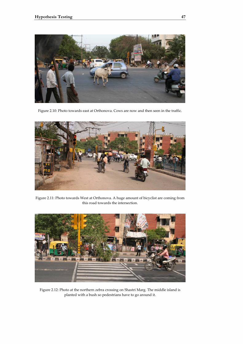
Figure 2.6 to Figure 2.12 show the intersection in pictures. Each picture will be explained and described one by one in the caption. The first figure is an ortho-photo while the six following figures are photographs.
Table 2.1: The cycle length at Orthonova is divided into five phases which varies during day and week. The alphanumeric codes refer to green light from the signal posts on Figure 2.5.
Phase no. 1 Phase no. 2 Phase no. 3 Phase no. 4 Phase no. 5 A1, A1r A1, A2 A2, A2r B1 B2
Table 2.2: Traffic counts from Orthonova in the morning peak hour from 9 am to 10 am. PCUs means Private Car Units. MTW: Motorized Two-Wheelers, TSR: Three-wheeled Scooter Richshaws. (Provided by TRIPP)
Leg Incoming flow Cars MTW TSR Bus/Truck Cycles PCUs North 505 359 134 82 165 1166 South 376 535 153 101 752 1445.5 East 346 499 260 48 385 1175 West 60 128 48 7 68 225 Total 1287 1521 595 238 1370 4011.5
Hypothesis Testing 45
A1A2
r
A2A1
r
B1
B2
A2rA2
A1r
A1
B2
B1
Shas
tri Ma
rg
Shas
tri Ma
rg
Figure 2.5: Plan of the signal boxes at Orthonova. The arrows and the alphanumeric codes represent the lights in the signal posts. Left turn on red is permitted.
Figure 2.6: Ortho-photo of Orthonova. Notice the residential area in the upper left corner, the office areas on the right side and the school in the lower left corner. (GoogleEarth 2006)

46 Traffic Calming in Delhi
Figure 2.7: Photo towards north at Orthonova. Notice the "shunt" lane to the left that merges with the service lane. The northbound lane has one bus lane and two car lanes.
Figure 2.8: Photo towards north at Orthonova. Notice the count down clock on top of the signal box in the middle of the picture. Count down clocks was installed in both directions
on Shastri Marg during the observation period.
Figure 2.9: Photo towards East at Orthonova. Traffic begins to grow late in the afternoon from around 5 pm and generally peaks between 7 and 8 pm.
Hypothesis Testing 47
Figure 2.10: Photo towards east at Orthonova. Cows are now and then seen in the traffic.
Figure 2.11: Photo towards West at Orthonova. A huge amount of bicyclist are coming from this road towards the intersection.
Figure 2.12: Photo at the northern zebra crossing on Shastri Marg. The middle island is planted with a bush so pedestrians have to go around it.

48 Traffic Calming in Delhi
2.3.2 Dilli Haat The traffic site named Dilli Haat is placed at Aurobindo Marg, which is one of the arterial roads that functions as connector between the centre of Delhi and south Delhi. Aurobindo Marg also connects the Inner Ring Road with the Outer Ring Road, see Figure 2.2. Thus a lot of through going traffic is passing Dilli Haat, which is located only few hundred meters north of the Inner Ring Road between a crafts market and the INA market. When the name Dilli Haat is used in this report, it refers to the traffic site and not to the crafts market which also is named Dilli Haat.
Figure 2.13 shows how Dilli Haat is located in relation to the (inner) Ring Road flyover, the crafts market and the INA market. The crafts market is south-west of Dilli Haat and INA market is direct east of Dilli Haat. While the crafts market is visited by many tourists, INA market mainly services the local Indians. At INA it is possible to buy everything from electrical gadgets to fresh fruit imported from abroad. On all sides of the markets residential areas are found. Figure 2.13 shows a four-armed intersection south of Dilli Haat – marked by a red dot. The map is a reprint from 2001
Figure 2.13: The traffic site Dilli Haat at Aurobindo Marg located north of the (inner) Ring Road flyover and between the crafts market Dilli Haat and the INA market. (Eicher 2006)

Hypothesis Testing 49
and since then that particular place has been redesigned. Aurobindo Marg has on the vast majority of its length a separation island between the two directions. Today this separation island has been extended so that only left turns are permitted from the two secondary roads south of Dilli Haat.
Dilli Haat is in this report the name for a pedestrian crossing between the two markets described above. Figure 2.14 shows the crossing and the nearest surroundings. In the upper left corner a small part of INA market is visible and in the lower right a small part of the crafts market is visible. The three numbers on Figure 2.14 refers to three typical places to cross the carriageways. Aurobindo Marg is divided by a physical separation island but in addition it also has a fence installed. At position (1) the fence has an 3,5 m wide opening. This is also the case at position (2) though no zebra marking is present here. At position (3) one crossbar in the fence is missing which provides an opening in the fence of not more than 40 cm. Aurobindo Marg has two car lanes and one bus lane in both directions which is marked by white painting. In addition there is a service road in both sides. These service roads mainly work as parking space for shoppers.
Table 2.3 shows a five-minute count of cars, motorized two-wheelers, TSRs, busses/trucks and bicycles. The counts are multiplied to represent one hour in the morning peak. When it is assumed that the peak hour equals 10 % of the AADT, it is found that Aurobindo Marg has an AADT – only cars – of 10 x (2424 + 1728) = 41,520 (both directions inclusive). Besides cars high numbers of motorbikes, TSRs and busses are represented. The AADT for all motor vehicles is 93.840. There are bus stops in both directions at Dilli Haat,
Figure 2.14: Technical base plan of the traffic site Dilli Haat. The pedestrian crossing connects INA market with the Dilli Haat crafts market. The north arrow is for guidance
only.

50 Traffic Calming in Delhi
and this generates a lot of pedestrian movement across Aurobindo Marg. The speed limit is 50 km/h for general traffic and 40 km/h for busses, trucks, TSRs and taxis (Delhi Traffic Police 2006c).
Figure 2.15 to Figure 2.22 show the intersection in pictures. Each picture will be explained and described one by one in the caption. The first figure is an ortho-photo while the six following figures are photographs.
Table 2.3: Traffic counts at Dilli Haat from on hour in the morning peak hour between 9 and 10 am. MTW: Motorized Two-Wheelers, TSR: Three-wheeled Scooter Richshaws.
Cars MTW TSR Bus/Truck Bicycle Towards north 2424 1368 708 240 24 Towards south 1728 1716 924 276 60
Figure 2.15: Ortho-photo of Dilli Haat. Notice the crafts market and the petrol station below in the picture and the INA market in the upper part if the picture. (GoogleEarth 2006)

Hypothesis Testing 51
Figure 2.16: Photo towards north at Dilli Haat. The zebra marking is at position 1 at Figure 2.14.
Figure 2.17: Photo towards south at Dilli Haat. Notice the fence in the separation island and the petrol station to the right.
Figure 2.18: Photo towards west at Dilli Haat. At group of pedestrians are waiting at the separation island to cross. The small grey car has been forced to stop by the man in white
shirt and with the arm raised.

52 Traffic Calming in Delhi
Figure 2.19: Photo towards west at Dilli Haat. Most pedestrians cross as a group.
Figure 2.20: Photo towards south at Dilli Haat. The man in the front is waiting to cross at the zebra marking. The group in the back is waiting to cross at position 2, see Figure 2.14.
Figure 2.21: Photo towards north at Dilli Haat. Four pedestrians are running to reach the separation island at position 2. The man to the left in red shirt is crossing at position 1, see
Figure 2.14.

Hypothesis Testing 53
Figure 2.22: Photo towards east at Dilli Haat. Only one cross bar is missing which provides an opening of less than 50 cm! Position 3 at Figure 2.14.
2.4 Methods for Data Collection During the field studies, the Swedish traffic conflict technique was the main method for collecting data. In addition speed measurements, behavioural studies and traffic counts were used.
2.4.1 The Swedish Traffic Conflict Technique The traffic conflict technique was “Invented” at General Motors by Perkins and Harris, developed at the Lund University in Sweden in the 1970s, and has been widely used since the 1980s. The general definition agreed upon for traffic conflicts is:
“A traffic conflict is an observable situation in which two or more road users approach each other in space and time to such an extent that a collision is imminent if their movements remain unchanged.” (Amundsen and Hyden 1977)
A further division between conflicts and “undisturbed passages” is illustrated in Figure 2.23. The figure does not necessarily illustrate the actual distribution between the events but gives an understanding of the thought behind the conflict technique. Basically the figure illustrates that the vast majority of all road user interaction happens as undisturbed passages, where road users are of no need of mutual communication. Further it says that conflicts can be divided into potential-, slight- and serious conflicts. The potential conflicts are occurring when there is ample time to do avoiding actions. Slight conflicts are occurring when there is rather small time and need of precise actions to do the avoiding actions. Serious conflicts are occurring when sudden and harsh actions are needed to avoid a crash. The figure show that some of the serious conflict leads to crashes/accidents. Actually the crash group can be divided into damage only, slight injury, severe injury and fatal crash. More general, conflicts can
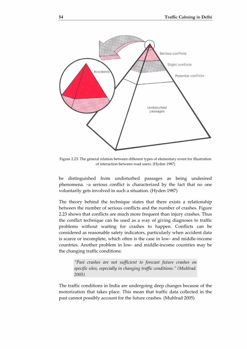
54 Traffic Calming in Delhi
Figure 2.23: The general relation between different types of elementary event for illustration of interaction between road users. (Hyden 1987)
be distinguished from undisturbed passages as being undesired phenomena. –a serious conflict is characterized by the fact that no one voluntarily gets involved in such a situation. (Hyden 1987)
The theory behind the technique states that there exists a relationship between the number of serious conflicts and the number of crashes. Figure 2.23 shows that conflicts are much more frequent than injury crashes. Thus the conflict technique can be used as a way of giving diagnoses to traffic problems without waiting for crashes to happen. Conflicts can be considered as reasonable safety indicators, particularly when accident data is scarce or incomplete, which often is the case in low- and middle-income countries. Another problem in low- and middle-income countries may be the changing traffic conditions:
”Past crashes are not sufficient to forecast future crashes on specific sites, especially in changing traffic conditions.” (Muhlrad. 2005)
The traffic conditions in India are undergoing deep changes because of the motorization that takes place. This mean that traffic data collected in the past cannot possibly account for the future crashes. (Muhlrad 2005)

Hypothesis Testing 55
When the traffic conflict technique is combined with traffic volume counts and speed measurements, it is possible to get a picture of the traffic problems occurring at a traffic site. This is advantageous when working on finding suitable and feasible countermeasures through diagnoses on specific areas or locations.
The distinguishing between serious and non-serious conflicts can be illustrated by the Speed-/Time to accident-graph, which is showed in Figure 2.24. Two factors define the threshold between serious and non-serious conflicts: Time to Accident (TA) and conflicting speed:.
⎯ Time to Accident (TA). The TA-value is the time that remains to an accident in the moment when evasive action has just started, presupposed that the road users continues with unchanged speeds and directions. The TA-value is calculated from the distance d and the conflicting speed v.
⎯ Distance (d). The d-value is the distance from the road user to the potential collision point, in the moment when evasive action has just started.
Figure 2.24: Graphical illustration of the connection between Time to Accident (TA) and speed. The curved line represents the borderline between serious and non-serious conflicts
recommended by the Swedish traffic conflict technique.
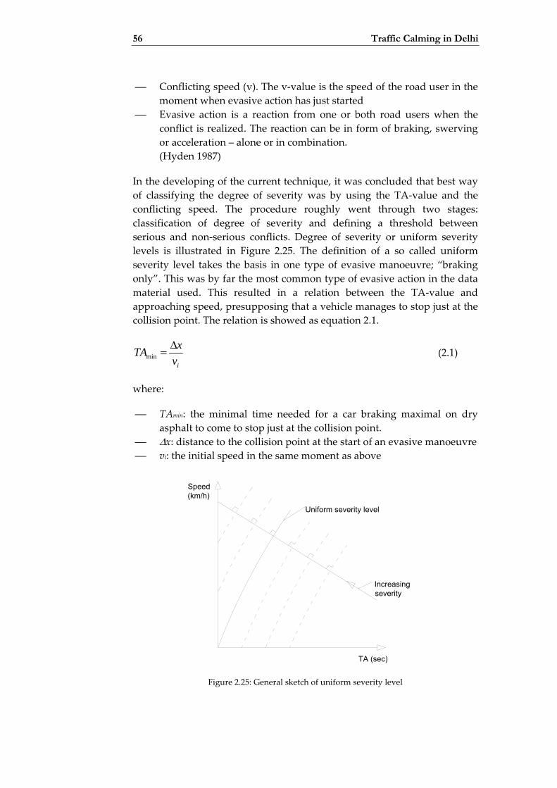
56 Traffic Calming in Delhi
⎯ Conflicting speed (v). The v-value is the speed of the road user in the moment when evasive action has just started
⎯ Evasive action is a reaction from one or both road users when the conflict is realized. The reaction can be in form of braking, swerving or acceleration – alone or in combination. (Hyden 1987)
In the developing of the current technique, it was concluded that best way of classifying the degree of severity was by using the TA-value and the conflicting speed. The procedure roughly went through two stages: classification of degree of severity and defining a threshold between serious and non-serious conflicts. Degree of severity or uniform severity levels is illustrated in Figure 2.25. The definition of a so called uniform severity level takes the basis in one type of evasive manoeuvre; “braking only”. This was by far the most common type of evasive action in the data material used. This resulted in a relation between the TA-value and approaching speed, presupposing that a vehicle manages to stop just at the collision point. The relation is showed as equation 2.1.
ivxTA Δ=min (2.1)
where:
⎯ TAmin: the minimal time needed for a car braking maximal on dry asphalt to come to stop just at the collision point.
⎯ Δx: distance to the collision point at the start of an evasive manoeuvre ⎯ vi: the initial speed in the same moment as above
Increasingseverity
Uniform severity level
TA (sec)
Speed (km/h)
Figure 2.25: General sketch of uniform severity level

Hypothesis Testing 57
The distance can be expressed as a function of the initial speed and the deceleration of the vehicle:
av
xavxxavv ififif 2
0,0,)(22
22 =Δ⇒<=−+= (2.2)
where:
⎯ vi: initial speed ⎯ vf: final speed ⎯ a: acceleration ⎯ xi: initial position ⎯ xf: final position
The friction force F can be expressed as:
gmnF ⋅⋅=⋅= μμ (2.3)
where
⎯ μ: friction coefficient ⎯ m: mass of the vehicle ⎯ g: gravitational acceleration
From equation 2.3 and Newton’s 2nd law it follows:
gaamgm ⋅=⇒⋅=⋅⋅ μμ (2.4)
From equation 2.1, 2.2 and 2.4 it follows:
gv
vav
vxTA i
i
i
i ⋅⋅=⋅=Δ=
μ21
2
2
min (2.5)
The friction coefficient can be described as a function of the mean speed:
)0306.0exp(85.0 mv⋅−⋅=μ (2.6)
This expression is only partially expressed by Hyden (1987). “0.85” is explained with a reference to the Swedish Road Directorate, but “-0.0306” is not explained. This has instead been estimated from the graphical representation of the severity level, see Figure 2.24 as an example. It is assumed by Hyden (1987) that the deceleration is linear and thus the mean speed during braking is half the initial speed. In addition a safety margin of half the necessary braking time is built in. Now it follows from equation 2.5 and 2.6:

58 Traffic Calming in Delhi
⎟⎟⎟⎟
⎠
⎞
⎜⎜⎜⎜
⎝
⎛
⎟⎠⎞
⎜⎝⎛ ⋅−⋅
=
i
i
v
vTA
210306.0exp7.16
5.1min (2.7)
From equation 2.7, a uniform severity level can be drawn in a TA-speed graph. From this level, parallel lines can be drawn to illustrate how the severity is increasing when “moving to the upper left”. This principle is showed on Figure 2.25. The above described severity definition was selected as the most appropriate definition from a total of five definitions. The comparison and selection was based on the following aspects:
⎯ Severity of conflicts ⎯ Severity of accidents ⎯ The proportion of accidents similar to conflicts for the different
severity definitions ⎯ The relevance of the combined conflicts and accident distribution
(Hyden 1987)
After having decided on a classification of degree of severity the next step is to defining a threshold between serious and non-serious conflicts. The result is showed in Figure 2.24. Originally the threshold was placed at a “lower” position “beginning” at 1.0 on the TA-axis. Later the threshold has been adjusted to the position in Figure 2.24. (Hyden 1987)
The entire work on developing the technique is based upon data material from Swedish cities. This means that the technique is fitted to a Swedish environment where the traffic composition is completely different from the situation in Delhi. In order not to be limited by that, a new subjective severity scale is made specific for the conflict studies in Delhi. A pre-arranged recording form from The Department of Traffic Planning and Engineering at Lund University is used for recording the observed conflicts. The conflict recording form is showed in Appendix B.
2.4.2 A New Severity Scale When observing the traffic in Delhi it was found necessary to use a subjective severity scale as a supplement to the severity definition used by CDBase (a software analysis tool described in the next chapter) and the Swedish traffic conflict technique. The subjective scale will in the next chapter be used to estimate whether the two factors used today as indicators – TA and speed – are adequate to distinguish between serious and non-serious conflicts in Delhi. Every observed conflict was given a number referring to the subjective scale. The scale is divided into 8 points. The first three are non-serious conflicts, the next three are serious conflict and the last two are crashes. The 8-point subjective scale is now described:

Hypothesis Testing 59
⎯ Non-serious conflict where normal interaction between the RUs – e.g. by using horn, light, swerving and/or braking – makes a crash to be considered as not a risk.
⎯ Non-serious conflict where evasive actions are needed to avoid a crash. Very low risk of crash to occur.
⎯ Non-serious conflict where an early evasive action is made and/or the speed is low. Low risk of crash to occur.
⎯ Serious conflict where an early evasive action is made and/or the speeds are low. One or both of the RUs make an evasive action that they not voluntarily would get involved in under normal conditions. Some risk of person injury if crash occurs.
⎯ Serious conflict where a late evasive action is made and/or the speed is high. Medium risk of person injury if crash occurs.
⎯ Serious conflict with contact or nearly contact between RUs after a late evasive action at high speed. No property damage or person injury. High risk of person injury.
⎯ Crash with property damage but no person injury ⎯ Crash with person injury
2.4.3 Speed Measurements As part of the work with the High Capacity Bus System (HCBS) TRIPP have gathered information about the speed at Shastri Marg and thus also at Orthonova. The speed has been divided into journey speed and running speed. Journey speed is a name for the speed of traffic in lines where road users are considered to be slowed down because of the presence of other road users. Running speed is a name for the speed of free road users where other road users not are having a delaying effect. Because of the existing speed data from Orthonova is divided in the two described categories, the speed at Dilli Haat will be measured likewise. Practically it will be done with a laser gun. Hundred measurements in both directions of respectively free vehicle and vehicle in line will ensure statistical useful values.
2.5 Collected Data After the traffic sites for data collection were decided on, a schedule for field studies was made. The schedule is showed as Appendix C. From the schedule it follows that traffic conflict studies were made four hours a day in five days for each of the two traffic sites. Initially the plan was to do studies in six hours in three days. However, when arriving to Delhi this had to be changed. During the day temperatures would vary between 35 and 45 degrees. This made outdoor field studies like the traffic conflict technique difficult because high concentration is needed to do the study. The solution was to do studies in the morning before 10 am – up to and in the peak hour – and again in the afternoon after 5 pm – the twilight would make it difficult to make observations later than 7 or 7.30 pm.
60 Traffic Calming in Delhi
Video recording equipment was not possible to borrow for the entire period of traffic conflict observations. Together with the fact that the observations was to be made by one person alone – no funds was reserved for education and use of a local observer team – it was decided not to use video recording in the traffic conflict observation periods.
The presentation of the entire data range from the traffic conflict observations will be made in the next chapter together with the analysis. The additional collected data are presented in the following appendixes:
⎯ Appendix D: Traffic counts at Orthonova ⎯ Appendix E: Traffic counts at Dill Haat ⎯ Appendix F: Speed measurements at Orthonova ⎯ Appendix G: Speed measurements at Dilli Haat ⎯ Appendix H: Example of conflict recording form from Orthonova
and Dilli Haat

Chapter 3
Data Analysis
The collected data that were introduced in the previous chapter will now be item for an analysis. The analysis will overall be split up into three parts; one regarding Orthonova, one regarding Dilli Haat and one regarding general observations. The main aim of the analysis is to make a diagnosis of problems for each of the two studied traffic sites. Additional the aim is to discuss whether a new threshold between serious and non-serious conflicts should be used for an Indian environment.
3.1 Analysis Method Besides of being involved in the development of the traffic conflict technique, Lund University has developed a software tool to help analysing collected conflict data. The software is called CDBase and is developed by Lars Ekman for Lund University. The version used for the analysis is version 1.901. The Swedish traffic conflict technique is incorporated in CDBase.
Figure 3.1 shows the welcome screen when CDBase is opened. The setup of the programme is very similar to the setup of the used conflict recording form that is showed in Appendix B. This makes it straightforward to copy the observed data from the recording form into CDBase. While every conflict recording form only holds information of one conflict, CDBase can store all the observed conflicts in one digital file (*.cdb). When all input is typed into the digital file, there are different types of output possible. The “output-window” gives the following possibilities:
⎯ Plotting of all conflicts in a speed-TA graph ⎯ Calculating the expected number of police reported injury crashes ⎯ Comparison of the speed in the conflicts
Besides, an LST-file is generated containing all the typed in information set up as a list. The LST-file can be opened with software made to handle spreadsheets. Figure 3.2 shows how CDBase can be useful, when wanting

62 Traffic Calming in Delhi
Figure 3.1: Screen shot of the welcome screen in CDBase version 1.901
Figure 3.2: Example of conflicts mapped onto a drawing of an analysed traffic site.

Data Analysis 63
to make a diagnosis of the occurring problems at a traffic site. CDBase can map the conflicts onto a drawing of the traffic site where conflicts between road users are showed as pair of arrows.
3.2 Data Analysis - Orthonova An introduction to the traffic site Orthonova is given in the previous chapter. The analysis in this section is divided up into three parts: Traffic Volumes, Speed and Traffic Conflicts.
3.2.1 Traffic Volumes As described earlier the main flow at Orthonova is the north-south direction; Shastri Marg. Appendix D shows a traffic count at the morning peak hour and the evening peak hour.
Looking at the morning peak hour it becomes very clear that there is a bicycle flow coming from south and east towards north, when comparing the income- and outcome flows. Also worth noticing is that the incoming flow of MTWs (Motorised Two-Wheelers) is greater than the flow of cars for three of the four legs; that is east, south and west. The incoming flow of MTW comes from east, south and west and goes towards north. Though the car traffic does not give a significant picture of a single flow direction, it is rather clear that the intersection in the morning moves light road users from south towards north and the centre of Delhi.
Looking at the evening peak hour it is more difficult to get at clear picture of flow directions. However, if cars and MTW are compared with the corresponding numbers from the morning, then it can be seen that a greater number is coming from north towards any of the other three directions. Also worth noticing is that the overall traffic has increased a little in the evening peak hour. The total number of vehicles has increased from 5030 in the morning to 5992 in the evening.
By using the data from the morning peak hour and the assumption that the peak hour represents 10 % of the AADT results in the following numbers translated into PCUs (Private Car Units):
⎯ AADT northern leg: 35,260 private car units (PCUs) ⎯ AADT southern leg: 25,455 PCUs ⎯ AADT eastern leg: 15,490 PCUs ⎯ AADT western leg: 3920 PCUs ⎯ AADT whole intersection: 40,115 PCUs.
3.2.2 Speed Appendix F shows speed measurements at Orthonova. The average speed of all road user groups are under the speed limit of 50 km/h. Information about the fractiles exceeding the speed limit was not possible to get.

64 Traffic Calming in Delhi
3.2.3 Traffic Conflicts This paragraph involves the results given from CDBase from the 20 hour conflict technique study at Orthonova. The subjective severity scale will be included in the analysis in section 3.5.
Figure 3.3 shows the speed-TA graph with all observed conflicts. A total of 50 conflicts were observed of which 37 were serious, which all ready has been explained. The figure shows that the observations include conflicts located above-, close to- and below the threshold, marked by the red curve.
Table 3.1 and Table 3.2 give an overview of the recorded conflicts at Orthonova. A total of 37 serious conflicts were recorded, in which only five did not involve VRUs. MTWs and cars are the groups involved in most conflicts. MTWs are involved in 68 % of the conflicts and make up 17 % of all passing vehicles in the morning peak hour. Cars are involved in 59 % of the conflicts and make up 16 % of all passing vehicles in the morning peak hour. The majority of conflicts with MTWs involve other MTWs or cars. Generally conflicts happen between protected road users and VRUs.
Figure 3.4 shows the mapping of conflicts on the base plan drawing. The area on the drawing is identical with the area for which the study was made. Besides showing the location of the conflicts in the intersection the figure also shows the movement of the involved road users. The colour of the arrows indicates the type of road user. The figure indicates that many conflicts happen between road users coming from two directions perpendicular to each other. This indicates that red light violations are a problem in the intersection.
Table 3.1: Overview of the serious conflicts (according to CDBase) observed during the observation period at Orthonova.
No VRUs included
Only VRUs included
Others Total
Serious conflicts 5 14 18 37
Table 3.2: Internal distribution of serious conflicts at Orthonova (according to CDBase)
Car MTW Bicycle Bus Lorry Pedestrian Car 3 11 4 1 1 2 MTW 8 4 0 1 1 Bicycle 1 0 0 0 Bus 0 0 0 Lorry 0 0 Pedestrian 0

Data Analysis 65
Figure 3.3: Speed-TA graph for all observed conflicts at Orthonova. Bikes (purple cross) also include MTWs. The red curve represents the threshold for serious and non-serious conflicts.
Figure 3.4: Mapping of serious conflicts at Orthonova (according to CDBase). Bold red arrows marked with a circle indicate a MTW. North is towards right.

66 Traffic Calming in Delhi
Figure 3.5 shows that speed of the faster of the two involved road users in conflicts are spread evenly between 10 km/h and 45 km/h. This gives the indication that speeds above the speed limit not are the causing factor for conflicts.
For all serious conflicts at Orthonova Table 3.3 shows the involved road users, the TA-value and the type of avoiding action. The two RU groups, cars and MTW, constitute each 16 avoiding actions. The average of the TA-value for cars is 0.7 seconds while the same value for MTWs is 0.5 seconds. The type of avoiding actions made by cars in 14 occurrences was “braking” and in 2 occurrences “braking + swerving”. For MTWs the type of avoiding actions was “braking” in 10 occurrences, “braking + swerving” in 5 occurrences and “swerving” one single time. “Acceleration” as an avoiding action was not observed.
Figure 3.5: Accumulated max speed of the two road users involved in a conflict (only serious conflicts according to CDBase definition)

Data Analysis 67
Table 3.3: Type of avoiding action for all serious conflicts at Orthonova from CDBase. The TA-value is measured in seconds.
Conflict no. Road Users Avoiding RU TA Type of avoiding action 1 MTW -Car MTW 0.5 Braking 7 MTW -MTW MTW 0.7 Braking 8 Car -Car Car 1 Braking + Swerving
11 Bike-MTW Bike 0.5 Braking 13 Bike-Bike Bike 0.3 Swerving 15 Car -MTW Car 0.4 Braking 16 Lor -Car Lor 0.4 Braking 17 Car -Car Car 0.7 Braking 18 MTW -MTW MTW 0.7 Braking 22 MTW -Bike MTW 0.7 Braking + Swerving 23 Car –Bike Car 0.9 Braking 24 MTW -MTW MTW 0.4 Braking + Swerving 25 Lor -MTW Lor 0.5 Braking 26 MTW -Car MTW 0.6 Braking + Swerving 28 Car -MTW Car 0.6 Braking 29 Car -Ped Car 0.6 Braking 30 Car -Ped Car 0.3 Braking 31 MTW -MTW MTW 0.4 Swerving 32 MTW -Bike MTW 0.4 Braking 33 MTW -MTW MTW 0.5 Braking 34 Car -MTW Car 0.6 Braking 35 Bus -Car Bus 1.2 Braking 36 MTW -MTW MTW 0.3 Braking + Swerving 37 MTW -Car MTW 0.4 Braking 38 MTW -Car MTW 0.3 Braking + Swerving 39 MTW -MTW MTW 0.4 Braking 40 Car -MTW Car 1.1 Braking 41 Car -MTW Car 1.2 Braking 42 Car -Car Car 0.8 Braking 43 Car –Bike Car 1 Braking 44 MTW -MTW MTW 0.7 Braking 45 Car -MTW Car 0.7 Braking 46 Car –Bike Car 0.4 Braking 47 Car -MTW Car 0.7 Braking 48 MTW -Ped MTW 0.2 Braking 49 MTW -Bike MTW 0.2 Braking 50 Car –Bike Car 0.5 Braking + Swerving
3.3 Data Analysis - Dilli Haat An introduction to the traffic site Dilli Haat is given in the previous chapter. The analysis in this section is divided up into three parts: Traffic Volumes, Speed and Traffic Conflicts.
3.3.1 Traffic Volumes The results from traffic volume counts at Dilli Haat are showed in Appendix E. The data reveals a clear hierarchy in the traffic composition. Cars are the dominating road user group followed by MTWs, TSRs,

68 Traffic Calming in Delhi
busses/trucks and bicycles. Still a relatively high number of motorized two-wheelers are present in both directions. In the morning peak hour in the south direction the number of MTW actually nearly are equal to the number of cars. When all motorized vehicles in both directions are summarized the AADT is about 80,700 motor vehicles (average for morning and peak hour). The number for the morning peak hour is 93,840 vehicles and for the evening peak hour 67,560 vehicles.
3.3.2 Speed Speed measurements at Dilli Haat were made using a hand held “laser gun”. The used model - “ProLaser Lidar Gun” - is able to isolate a single vehicle out of a group. The measurements were made on a Wednesday between 8 and 9 am and again between 5 and 7 pm. Table 3.4 shows the results. It was desired to record 100 values before calculating an average value. This was, however, not possible for the “running speed” towards north. Only 27 vehicles were measured during a period of two hours. This clearly indicates that the traffic composition exists of a very small part of free vehicles. The measurements were made just before the morning peak hour and the evening peak hour with reference to be able to measure both journey speed and running speed. The average speeds show that the traffic is very near or below the speed limit of 50 km/h. Only towards south the 85 % fractile for running speed exceeds the speed limit.
Table 3.4: Results from the speed measurement at Dilli Haat. The average values are each calculated from 100 speed measurements except for “running speed” towards north, where only 27 measurements are the basis.
Towards North (between 5 and 7 pm)
Towards South (between 8 and 9 am)
Journey Speed Running Speed Journey Speed Running Speed [km/h] [km/h] [km/h] [km/h] Average 32 44 39 53 85 % frac. 39 50 45 60
3.3.3 Traffic Conflicts This paragraph involves the results given from CDBase from the 20 hour conflict technique study at Dilli Haat. The subjective severity scale will be included in the analysis in section 3.5.
Figure 3.6 shows the speed-TA graph with all observed conflicts. A total of 24 conflicts were observed of which 15 were serious, which already has been explained. The figure shows that the observations include conflicts located above-, close to- and below the threshold, marked by the red curve.
Table 3.5 and Table 3.6 give an overview of the recorded conflicts at Dilli Haat. A total of 15 serious conflicts were recorded, of which 2 did not

Data Analysis 69
involve VRUs and 2 involved only VRUs. Because Dilli Haat first of all is a pedestrian crossing it is expectable that the majority of the conflicts are involving pedestrians. More than 80 % of the conflicts are involving pedestrians and the vast majority is with cars.
Figure 3.6: Speed-TA graph for all observed conflicts at Dilli Haat. Bikes (purple cross) also include MTWs. The red curve represents the threshold between serious and non-serious
conflicts.
Table 3.5: Overview of the serious conflicts (according to CDBase) observed during the observation period at Dilli Haat.
No VRUs Only VRUs Other Total Serious conflicts
2 2 11 15
Table 3.6: Internal distribution of serious conflicts at Dilli Haat (according to CDBase)
Car MTW Bicycle Bus Lorry Pedestrian Car 1 1 0 1 0 10 MTW 0 0 0 0 2 Bicycle 0 0 0 0 Bus 0 0 0 Lorry 0 0 Pedestrian 0

70 Traffic Calming in Delhi
Figure 3.7 shows the mapping of conflicts on the base plan drawing. The area on the drawing is identical with the area for which the study was made. Besides showing the location of the conflicts at the traffic site the figure also shows the movement of the involved road users. The colour of the arrows indicates the type of road user. The figure shows that most of the conflicts happen near the zebra marking.
Figure 3.8 shows that speed of the faster of the two involved road users in conflicts are spread between 15 km/h and 45 km/h. Round 85 % of the conflicts have max speeds lower than 35 km/h.
For all serious conflicts at Dilli Haat Table 3.7 shows the involved road users, the TA-value and the type of avoiding action. The most observed avoiding action is “Braking” – observed 7 times – while “Braking + Swerving”, “Swerving” and “Accelerating” are observed respectively 2, 4 and 2 times.
Figure 3.7: Mapping of serious conflicts at Dilli Haat (according to CDBase). Bold red arrows marked with a circle indicate a MTW. North is towards left.

Data Analysis 71
Accumulated max speeds
CDBase (1.901)for LTH Lund University
Km/h50454035302520151050
%100
90
80
70
60
50
40
30
20
10
0
Figure 3.8: Accumulated max speed of the two road users involved in a conflict (only serious conflicts according to CDBase definition)
Table 3.7: Type of avoiding action for all serious conflicts at Dilli Haat from CDBase. The TA-value is measured in seconds.
Conflict no. Road Users Avoiding RU TA Type of avoiding action 5 Car -Ped Car 0.5 Braking 8 Car -Car Car 0.6 Braking
10 MTW -Car MTW 0.4 Braking + Swerving 11 Ped -Car Ped 0.2 Accelerating 12 Ped -Car Ped 0.4 Swerving 13 Car -Bus Car 1.2 Braking 14 MTW -Ped MTW 0.5 Swerving 15 Car -Ped Car 0.7 Swerving 17 Car -Ped Car 0.6 Braking 18 Car -Ped Car 0.6 Braking 19 Car -Ped Car 0.7 Braking 20 Car -Ped Car 0.4 Braking 21 MTW -Ped MTW 0.7 Braking + Swerving 22 Car -Ped Car 1 Swerving 24 Ped -Car Ped 0.2 Accelerating
3.4 Data Analysis - General observations In addition to the traffic conflict analysis above some general observations are worth mentioning. This section is divided into observations regarding physical design, road user behaviour and road user’s willingness of risk.
3.4.1 Physical design Humps and bumps are already used widespread in Delhi. Six different types were observed. Two of the bumps are showed in Figure 3.9 and Figure 3.10. The bumps are a combination of two or three small bumps in combination and can result in intense vibrations of the crossing vehicle.

72 Traffic Calming in Delhi
Figure 3.11 illustrates the six different types of humps/bumps that were observed. The first two were observed with the same height that is 10 cm. The next three have lower heights – between 5 and 10 cm – and varies by the number of bumps that are combined; one, two or three. The last bump illustrated in the figure is constructed as a trapezium with a change in surface on the top, e.g. cobble stone. The height is about 10 cm and the length of it can vary from place to place.
Figure 3.9: A triple bump. The rear wheel of the scooter is without contact with the asphalt. This type of bump also slows down the speed of MTWs. Other light vehicles – like TSRs –
have to slow down the speed greatly to cross and still with some inconvenience.
Figure 3.10: A double bump. The driver is without contact with the seat. The only vehicle type that was observed crossing the bump without slowing down the speed was a heavy
four-wheel-drive vehicle with soft suspension. The combination of high speed, soft suspension and heavy weight resulted in little influence from the bump.

Data Analysis 73
3 m
Figure 3.11: Six different types of humps/bumps were observed in Delhi. –Longitudinal section. The length measure is for guidance only.
The condition of the road surface is at many places in bad condition and forces road users sporadically to slow down speed. Other places – like showed on Figure 3.12 – the road condition on a longer stretch is bad or paved with an uneven material. Because of the inconvenience from these kind of road conditions the speed decreases.
Bus lanes are widespread on arterial roads. This often results in roads that have very wide sections. A carriageway with two car lanes and a bus lane will in some situations of high traffic operate as a three lane road, because TSRs and MTWs – beside the busses – use the bus lane. In addition the bus lane can make the carriageway look wide and safe and thus encourage for high speeds.
Figure 3.12: Press Enclave Road in the southern part of Delhi. The carriageway towards east is covered with cobblestones.

74 Traffic Calming in Delhi
The speed limit in Delhi is divided into three levels: 60/40, 50/40 and 40/30 (all in km/h). The speed limit is differentiated between two groups:
⎯ High speed: Jeeps Car and Two-Wheeler ⎯ Low speed: All transport vehicles including TSR/Taxi
(Delhi Traffic Police 2006c)
In the majority of Delhi the speed limit is 50/40 km/h, see Figure 3.13. In reality the differentiation is not working. Transportation vehicles are mixed with all other vehicles and follow the flow. Neither seem the speed to be lower in the bus lane.
Figure 3.13: The speed sign show how the speed limit is differentiated. In reality this is not followed
3.4.2 Road User Behaviour All road users are divided into a hierarchy; “the biggest and strongest always has the right of way and the smaller has to yield”. This seems to be generally accepted by all road users. The hierarchy sets in when two road users meet, e.g. a car and a pedestrian at a pedestrian crossing: If the car is first at the meeting point it will “win”. If they come to the point at the same time the car will “win”. If the pedestrian comes a little before the car then the car will “win”. Only if the pedestrian comes well before the car, the pedestrian will “win”. Most pedestrians accept that they are the weak part compared with the motor vehicles. This is also the case at pedestrian crossings. Formally, pedestrians have the right of way:
“Pedestrian Crossings. These are alternate black and white stripes painted parallel to the road generally known as zebra crossing. Pedestrians must cross only at the point where these lines are provided and when the signal is in their favour at controlled crossings. You must stop and give way to pedestrians at these

Data Analysis 75
crossings. Pedestrian crossings are marked to facilitate and give the right of way to pedestrians.” (Delhi Traffic Police 2006b)
Because of the hierarchy most pedestrians waiting to cross a zebra crossing until a small group of pedestrians have gathered at the side of the road. Typically they will wait a while for a gap big enough to cross. If such one does not appear one from the group slowly will start to move out on the road and try to stop the vehicles. Then, when the traffic is stopped, the rest of the group will follow, see Figure 3.14. This will lead to kind of “controlled” conflicts where the pedestrians are aware of potential conflicts / crashes. The traffic can in addition to the hierarchy also be described by a busyness, which often comes to expression through the use of horns. Every single free square meter of asphalt must be used – seems to be the thought. The busyness in the traffic stands in contrast with the more relaxed attitude in the social life in general.
As described earlier the traffic composition in Delhi consists of many different road user groups. This mix of road users leads to a kind of less strict use of lane, in the situation of more than one lane. Cars, seems to be the only group of road users that follows the lanes. Particularly MWTs and partially TSRs do not follow the marked lanes because of the possibility of swerving and finding small gaps where cars are too big to pass. Another aspect is how the busses use the bus lanes. Figure 3.15 shows how busses often stop halfway onto the bus lane and halfway onto the car lane.
Red light violations can often be observed in small, signalized intersections. It does not have to be a rash action. Often a vehicle stopping for red will check for crossing vehicles, and if no other vehicles are approaching the intersection, the first vehicle will enter it.
Figure 3.14: Often pedestrians wait until they are a small group gathered before they start to "force" their way out on the carriageway, like here at Dilli Haat.

76 Traffic Calming in Delhi
Figure 3.15: The bus lane is often used by many others than busses.
3.4.3 Willingness of Risk As described in the previous section pedestrians often force their way across the carriageway. If a gap does not appear or the traffic is not willing to stop, the time gap accepted for pedestrians to cross might fall. This will lead to either running across the carriageway or taking one lane at a time. In both examples small time gaps can be accepted. Generally the traffic in Delhi can be described in three different ways (see Figure 3.16): Pulse traffic, Platoon traffic and traffic where pedestrians have to force their way. When the traffic comes in “pulses”, crossing pedestrians are willing to wait for a time gap big enough. When the traffic comes in “platoons”, crossing pedestrians will be more willing to use the first time gap that appears even though it may be little. When traffic comes in on stream without gaps, crossing pedestrians will have to force their way as described above.
Pulse traffic
Platoon traffic
Pedestrians force their way
Figure 3.16: Three types of traffic typical for Delhi.

Data Analysis 77
Figure 3.17 shows how cars also are willing to accept small spaces. By tipping the side mirror to the side it will be possible to get closer to the vehicles next to without contact.
Figure 3.17: Small spaces between vehicles are generally accepted. To be able to get really close together many cars have their side mirror tilted towards the side of the car, like these
three cars.
3.5 Threshold between conflicts As it was explained in the previous chapter a subjective severity scale was introduced and used during the conflict observations. The general differences in the observations are illustrated in Table 3.8 and Table 3.9. The fist clear difference is the total number of serious conflicts. At Orthonova only 15 serious conflict (CDBase: 37) were observed according to the subjective scale. At Dilli Haat 7 serious conflicts (CDBase: 15) were observed. This means that about half of the observed serious conflicts are tossed away when the subjective severity scale is used. In addition to this it must be mentioned, that a smaller number of conflicts have been tossed away during the observations. These conflicts would all be close to the
Table 3.8: Serious conflicts at Orthonova
No VRUs Only VRUs Other Total CDBase 5 14 18 37
Subjective scale
3 5 7 15
Table 3.9: Serious conflicts at Dilli Haat
No VRUs Only VRUs Other Total CDBase 2 2 11 15
Subjective scale
1 0 6 7

78 Traffic Calming in Delhi
threshold between serious and non-serious conflicts according to CDBase. The reason for tossing them away was that actions made by the road users – that could be seen as evasive actions – not were observed as an “undesired phenomenon” but rather a normal action. At some observed “conflicts” it hence was estimated that the linguistic definition – an “undesired phenomena” – should be given more weight than the technical definition used in CDBase. Because of this, a smaller number of “conflicts” was not even recorded. The linguistic problem here is taking its basis in the fact that the road users don’t stop using the road network because it is linked with risk of crash. Instead the road users accept this risk and if the risk level does not change to the better, they will start to see the risk as a normal part of “using the road network”. The risk will not turn into a “desired” phenomenon but rather an “undesired” phenomenon.
The differences are also illustrated on Figure 3.18 to Figure 3.21 on page 80 and page 81. The figures show the serious conflicts plotted in the Speed-TA diagram. In all four diagrams the threshold between serious and non-serious conflicts according to CDBase are illustrated by the curve in the diagram. Figure 3.18 and Figure 3.19 show data from Orthonova. The first shows the 37 serious conflicts from CDBase while the second shows the 15 serious conflicts according to the subjective severity scale. When the two diagrams are compared it becomes clear that the most evident differences are in the area of the diagram where speed equals 40 km/h and TA equals 1 s. In this area with relative high speeds and TA-values the subjective scale tosses away the conflicts. It can not be concluded from the two figures alone that the threshold should be moved to a higher – leftwards and upwards – position to represent the subjective severity scale. Figure 3.20 and Figure 3.21 show data from Dilli Haat. The first shows the 15 serious conflicts from CDBase while the second shows the 8 serious conflicts according to the subjective severity scale. When comparing these two diagrams it should first of all be clear that the data range is smaller than for the data at Orthonova. Still it should be noticed how the data in the second diagram generally is lying at a higher severity level – more leftwards and upwards except for one conflict – compared with the first diagram.
When the original severity definition for the Swedish traffic conflict technique was defined the following items were part of the discussion:
⎯ Distance in space, to collision point ⎯ Distance in time, to collision point ⎯ Deceleration power needed to avoid an accident ⎯ Type of road user ⎯ Speeds of the road users ⎯ Manoeuvre type (Hyden 1987)

Data Analysis 79
It is not the aim of this report to change the basics of the Swedish traffic conflict technique. Still it would be of interest to dwell with some of the basic problems of a severity rating. The conflict technique is “only” using conflicting/approaching speed and the TA-value to decide whether a conflict is serious or non-serious. Item number four and six in the list above is interesting – especially with motorbikes in mind. When motorbikes approach other slower moving road users, conflicts often seems to be unavoidable. The severity however often will be lover than CDBase will come up with. Motorbikes most often have space to make a swerving manoeuvre instead of braking. Between 24 % (Orthonova) and 40 % (Dilli Haat) of the observed conflicts involved swerving as the type of evasive action. As it was explained in the previous chapter, the conflict technique is build upon the most typical manoeuvre in an evasive action that is braking. If a definition of severity was made specific for the use in India, it probably would have to include something about motorbikes and the possibility of swerving.
The serious conflicts that were tossed away are showed in Table 3.10 and Table 3.11 on page 82. At Orthonova the avoiding road user in 11 of the serious conflicts were MTWs. In nine of the serious conflicts it was cars. The type of evasive action varies but with an overweight to “braking”. 21 of the serious conflicts at Orthonova that was tossed away involved “braking” as an evasive action. At Dilli Haat the avoiding road users were four cars, two pedestrians and two MTWs. The type of evasive action varies. At both Orthonova and Dilli Haat the conflicts that are tossed away seems to be evenly distributed at all the road users and types of evasive action.
The total data range dos not seems to give a clear or unambiguous answer to the questions whether:
⎯ the shape of a uniform severity line should be changed ⎯ the threshold between serious and non-serious conflicts should be set
at a higher position – more leftwards and upwards in the speed-TA graph
Though it has been argued for that “swerving MTWs” not adequately is included in the Swedish traffic conflict technique, it also should be mentioned that predominant evasive action made was “braking”. This is in reasonable agreement with how the shape of the uniform severity line was determined. This indicates that the shape of the threshold – not the position but only the shape of the curve – is usable in this study.

80 Traffic Calming in Delhi
Figure 3.18: Serious conflicts at Orthonova according to CDBase. Because of overlapping dots only 23 of the 37 conflicts can be counted on the diagram.
Figure 3.19: Serious conflicts at Orthonova according to the subjective severity scale. Because of overlapping dots only 13 of the 15 conflicts can be counted in the diagram.

Data Analysis 81
Figure 3.20: Serious conflicts at Dilli Haat according to CDBase. Because of overlapping dots only 13 of the 15 conflicts can be counted in the diagram.
Figure 3.21: Serious conflicts at Dilli Haat according to the subjective severity scale. Because of overlapping dots only 7 of the 8 conflicts can be counted in the diagram.

82 Traffic Calming in Delhi
Table 3.10: 22 serious conflicts at Orthonova are tossed away when using the subjective severity scale
Conflict no. Road Users Avoiding RU TA Type of avoiding action 1 MTW -Car MTW 0.5 Braking 8 Car -Car Car 1 Braking + Swerving 7 MTW -MTW MTW 0.7 Braking
18 MTW -MTW MTW 0.7 Braking 22 MTW -Bike MTW 0.7 Braking + Swerving 23 Car -Bike Car 0.9 Braking 24 MTW -MTW MTW 0.4 Braking + Swerving 25 Lor -MTW Lor 0.5 Braking 26 MTW -Car MTW 0.6 Braking + Swerving 28 Car -MTW Car 0.6 Braking 29 Car -Ped Car 0.6 Braking 31 MTW -MTW MTW 0.4 Swerving 32 MTW -Bike MTW 0.4 Braking 33 MTW -MTW MTW 0.5 Braking 34 Car -MTW Car 0.6 Braking 35 Bus -Car Bus 1.2 Braking 39 MTW -MTW MTW 0.4 Braking 40 Car -MTW Car 1.1 Braking 41 Car -MTW Car 1.2 Braking 43 Car -Bike Car 1 Braking 44 MTW -MTW MTW 0.7 Braking 50 Car -Bike Car 0.5 Braking + Swerving
Table 3.11: 8 serious conflicts at Dilli Haat are tossed away when using the subjective severity scale
Conflict no. Road Users Avoiding RU TA Type of avoiding action 5 Car -Ped Car 0.5 Braking
12 Ped -Car Ped 0.4 Swerving 13 Car -Bus Car 1.2 Braking 14 MTW -Ped MTW 0.5 Swerving 15 Car -Ped Car 0.7 Swerving 21 MTW -Ped MTW 0.7 Braking + Swerving 22 Car -Ped Car 1 Swerving 24 Ped -Car Ped 0.2 Accelerating
What the collected data, however, does tell is:
⎯ It is relevant to work with a subjective severity scale to be able to remove those conflicts that is problematic in CDBase.
⎯ The used subjective severity scale together with the original severity scale introduced by Hyden (1987) could result in a more usable (and sustainable) scale.
⎯ The change – when only using the subjective severity scale – on the diagnosis is minimal.

Data Analysis 83
When ”only” using the collected data for a diagnosis of problems at the observed traffic sites, the difference in using all the serious conflicts or only those selected by the subjective severity scale is minimal. If the aim, however, was to examine for a correlation between serious conflicts and injuries, the effect most likely would have been more visible.
3.6 Diagnosis of Problems This section is giving a conclusion to the conflict technique analyses that were made above. The conclusion will take the form of a diagnosis of problems at Orthonova and Dilli Haat. In addition to using the conflict analysis data, the findings from the previous section will also be included, thus taking into account the findings from the use of the subjective severity scale.
3.6.1 Orthonova The majority of the conflicts, that have been recorded, include road users from two on each other perpendicular directions. Often one of the road users come from the eastern leg and the other road user comes from either the northern or the southern leg. The explanation of this kind of conflicts is red light violations. It results in perpendicular conflicts. The positions of the conflicts in the intersection are mainly where the west bound lanes cross with the north bound lanes and the south bound lanes.
The reason behind the red light violations are a combination of the hierarchy among the road user groups, the non-observance of the signalization at Orthonova and the busyness of the traffic.
Cars and MTWs are the involved parts in the majority of the conflicts. Cars and MTWs are also the road user groups that most often are the avoiding road user (takes evasive action).
The lack of proper channelization – for instance for right turning vehicles – makes the turning manoeuvres more complex to foresee. Generally, the layout of the intersection does not help particularly to give clearness of who has right of way, and where the right position is for which manoeuvres.
3.6.2 Dilli Haat The most obvious problem is the lack of willingness of motor vehicles to stop for crossing pedestrians. This is not just the case at high speeds. Also at low speeds, motor vehicles tend to continue to pass through the zebra crossing without stopping. This mainly seems to be caused by the hierarchy in the traffic. A secondary cause is the relative simple marking of the crossing. No signs or physical or visual measures – except for the painted zebra strips on the asphalt – mark the crossing.
84 Traffic Calming in Delhi
Cars and pedestrians are the involved parts in the majority of the conflicts. Cars are the road user groups that most often are the avoiding road user (takes evasive action).
Pedestrians have to cross three lanes before they reach the middle island / the sidewalk. This results in, that some pedestrians take one lane at a time and wait in the small space between two lanes for the next time gap. This indicates, that the physical design not is providing the proper crossing possibilities compared with the pedestrians’ needs.
Chapter 4
Results
The chapter will concern analysis results from traffic conflict studies made in Delhi. The majority of the chapter will concern the study that was analysed in the previous chapter. To begin with, however, a traffic conflict study made by IIT will be discussed. This will be done with the aim of giving a better view of the possibilities and limitations that traffic conflict technique gives when used in Delhi. Afterwards it will be discussed how the Swedish traffic conflict technique in further studies can and should be used. The rest of the chapter will take its basis in the previous chapter analysis results together with the Danish design rules of traffic calming. The Danish design rules will first be presented and since be used when giving proposals of measures of traffic calming at Orthonova and Dilli Haat. To end with, the findings regarding traffic calming will be lifted to a general level. This will result in a prognosis the present traffic calming measures useable in Delhi and not only at Orthonova or Dilli Haat.
4.1 Existing experiences with traffic conflict technique In the 1990s IIT did a comprehensive traffic conflict technique study in Delhi (Tiwari et al. 1998). The aim of the study was to examine whether the mainly positive results from similar studies in high-income countries also could be achieved in Delhi. The approach was rather sceptical because:
“…the design of traffic conflict technique reflects the situation in relatively homogeneous traffic.” (Tiwari et al. 1998)
14 traffic sites – representing “high“, “moderate“ and “low“ numbers of fatalities over a period of one year – were selected for the study. The selection involved two stages. First all streets in Delhi were divided into “high level”, moderate level” or “low level” of fatalities based on data from police reports from a three year period. The second stage included specific traffic fatality information. Only mid-block fatalities were included and they were divided into “high”, “moderate” and “low” concentrations. A comparison was made between the streets and fatality rates. If the rank of the street matched the rank of a fatality site on the same street, the site was

86 Traffic Calming in Delhi
selected for the further study. This selection process was made to make up for a possible regression to the mean effect, and for not to base the study on traffic sites with high fatality rates alone.
Traffic conflict studies were made at the 14 mid-block sites. The definition of a conflict was kind of broad / weak:
“When an entity made an abrupt change of direction or noticeably slowed within the street segment, observers noted the entity type directly causing the response and the type of conflict on their conflict tally sheets.” (Tiwari et al. 1998)
This definition is very weak with respect to the level of severity in a conflict. It indicates, that the number of conflicts recorded will be higher that with the Swedish traffic conflict technique. Road user flow rates and average speeds at the sites also were decided. The conflict counts were converted into rates involving dividing the counts by the site’s observation time and mid-block segment length. By converting the conflict data – from the 14 sites – it becomes possible to compare them individually and thus rank them. The fatality data – from the same 14 sites – is also ranked. The study uses the rank of conflicts and fatalities at the 14 sites to control the correlation between the traffic conflict technique and fatal crashes. It is found that:
“The ranking of the site changes for different combinations of conflict types…” and “…the ranking also changes for (…) traffic modes.” (Tiwari et al. 1998)
Further it is concluded that conflict data alone can not be used for reducing daytime, mid-block fatalities in Delhi. This is because conflict data do not correlate with fatality data. Still it is concluded, that the data give an understanding of the road user behaviour in the heterogeneous traffic of Delhi. (Tiwari et al. 1998)
The procedure of using rank between sites to compare conflict data with fatality data is not in accordance with the original Swedish traffic conflict technique. By using the rank a lot of precision is lost. The fatality data is relatively small compared with the conflict data. This means that the 14 sites can not be divided into 14 different ranks. In the comparison made the fatality data divides the 14 sites into maximum 11 ranks and minimum 2 ranks.
The Swedish technique – as it is used in CDBase – uses three categories for comparing: car – car (angle), car – car (frontal or rear-end) and car – VRU. In these three categories the corresponding numbers of conflicts are converted into an “expected number of police reported injury accidents per

Results 87
year”. This procedure would be of interest in order to study how good results the in-built conversion factors in CDBase are with relation to an Indian injury-picture. In this context it is important to mention that the Swedish technique only deals with a relationship between serious conflicts and injury accidents – not fatalities. (Hyden 1987)
The study made at IIT does not mention anything about the threshold between serious and non-serious conflicts. This was pointed out when the definition of a conflict was showed above. Instead it deals with the problem of having reliable crash data. The choice of looking at fatal crashes and not injury crashes was because of under reporting:
“This study of the relationship between conflicts and fatal crashes was attempted because many Delhi roadway users do not report non-fatal crashes.” (Tiwari et al. 1998)
It is estimated that the fatal crash statistics of Delhi are reliable. According to earlier studies fatal crash data in India generally suffer from only 5 % under reporting. When it comes to injuries, the statistics probably are underreporting the number of injuries by more than a factor of two (Mohan 2004). No matter what kind of data the conflict data is compared with, a deviation must be expected. In this case a confidence interval must help to decide whether the deviation is systematic and lies within the acceptable marginal values. When comparing conflicts with fatal crashes – as it is done in the IIT study – the deviation must be expected to be visible. The level of uncertainty becomes higher when conflicts with low severity are compared to fatal crashes. Thus it is desirable to use conflict data with a high severity in comparison with crash data (not only fatalities). The difference in the method used in the IIT study and the method from the Swedish TCT is showed in Figure 4.1. The figure shows how the IIT study tries to find correlation between conflicts defined very broad and the small group of fatalities. The Swedish TCT is using a more well-defined group of serious conflicts to find correlation with crashes (not only fatalities). The level of uncertainty must be considered high when using the procedure from the IIT study.
The study made at IIT shows that traffic conflict studies can give a useful understanding of the traffic situation in the heterogeneous traffic of Delhi, though no correlation with fatalities was found. The study concludes that conflict technique can be used to improve “traffic management” and as a part therein traffic calming is a measure. This report does not concern injury data, but instead uses conflict data to give diagnoses of traffic problems. It is estimated that this lies in extension of the conclusion from IIT and within the demonstrated field of action.

88 Traffic Calming in Delhi
Swedish serious conflicts
Swedish crashes
Indian fatalities
Indian conflicts
Undisturbed passages
Figure 4.1: Illustration of the differences in the data that the IIT study and the Swedish TCT try to find correlation between.
4.2 The Swedish traffic conflict technique In the previous chapter it was discussed how the use of a subjective severity scale influences the results of a traffic conflict technique study. It was found - for the study made specific for this report – that the subjective severity scale not had an influence on the diagnoses of problems given at Orthonova and Dilli Haat. On the other hand it has not been demonstrated that the use of a subjective severity scale is without significance. By using such a scale it will be possible to examine if a certain type of conflicts is irrelevant. Here, two kinds of conflicts immediately are of interest: Conflicts involving pedestrians and conflicts involving MTWs. Shbeeb (2000) has stressed that the Swedish TCT seems to treat conflicts where pedestrians are the avoiding road user less severe than they are. Another problem with the Swedish TCT that is discussed in this report is about swerving MTWs. These actions, seems to be treated more severe by Swedish TCT than they are. A subjective severity scale can help to clarify these possible problems.
This particular traffic conflict study made for this report has not aimed at finding a correlation between serious conflicts and crashes. If doing so, it certainly will be interesting to use a subjective severity scale. This can help in the attempt of re-positioning the threshold in the TA-speed graph. The used severity scale - that was introduced in chapter 2 - operated with three non-serious levels, three serious levels and two where a crash was involved. The practical experiences from the study say that the first three levels have too little spacing while the spacing between serious conflict and

Results 89
crash is too big. Hyden (1987) earlier have introduced another severity scale also in 8 levels:
⎯ Undisturbed passage ⎯ Potential conflict ⎯ Slight conflict ⎯ Serious conflict, type 1 ⎯ Serious conflict, type 2 (touching) ⎯ Serious conflict, type 3 (hitting) ⎯ Serious conflict, type 4 (hitting) ⎯ Serious conflict, type 5 (collision)
These two severity scales is below mixed into one scale. It is done with the aim of making a subjective severity scale that is build on the best from the two scales discussed above. Further it is the aim to make the formulations as precise as possible in order to make it useful in the mixed traffic streams in Delhi. The scale has thus not been used or tested in practice, but it is a result of the findings from the practical study in Delhi. The subjective severity scale is a suggestion that can be used in further TCT studies:
⎯ Undisturbed passage. None of the road users involved is influenced in behaviour due to the other road user’s presence.
⎯ Non-serious potential conflict. At least one of the road users changes speed or direction in very ample time.
⎯ Non-serious slight conflict. Potential risk of a serious conflict. At least one of the road users takes evasive action. It involves events where one of the road users “takes a chance” or accepts a fairly small gap without complete control of all possible intersecting road users.
⎯ Serious conflict. An early evasive action is made and/or the speeds are low. The interaction between the road users has broken down for a short moment.
⎯ Serious conflict. A late evasive action is made and/or the speed is high. The interaction between the road users has broken down and at least one of the road users become highly surprised and is forced to take immediate action.
⎯ Serious conflict, “touching”. At least one of the road users involved acts late or performs poorly. The road users touch or nearly touch each other. No property damage.
⎯ Serious conflict, “hitting”. The road users are hitting each other with almost the approach speed. Property damage but no person injury.
⎯ Serious conflict, “crash”. The road users are colliding without time to start an evasive action. Person injury

90 Traffic Calming in Delhi
4.3 Danish Design Rules of Traffic Calming The Danish design rules of traffic calming include a list of feasible measures. This list will be introduced, explained and discussed. Pros and cons with respect to use of these measures in the traffic situation at Orthonova and Dilli Haat will be set up. The Danish design rules of traffic calming represents a wide range of possibilities, from measures with only visible effect to measures with physical discomfort – if not following the speed limit. A total of 14 different types of measures are included. (Danish Road Directorate 2006)
Basically, the conditions for implementing traffic calming measures are problems with speed and/or problems with feeling unsafe. Another condition could be problems with crashes.
4.3.1 14 types of traffic calming measures A short introduction to each of the types as they are described in the Danish design rules (Danish Road Directorate 2006) are given below.
1) Prior notice – has to ensure that road users not are surprised by subsequently traffic calming measures. Signs, plantation, lighting and rumble strips can be used. See Figure 4.2.
2) Gateways – has to mark the change from one speed limit to another lower limit. They can be used between the rural area and urban area. The measure often is visual by using plantation, change of pavement, lighting or portals. See Figure 4.3.
3) Hump – can be used on arterial roads as well as local roads with speed limits at 50 km/h or below. Circle Humps or sinus Humps are the most common used. Humps have a good speed reducing effect. See Figure 4.4.
4) Elevated surface - can be used on arterial roads as well as local roads with speed limits at 50 km/h or below. The name “elevated surface” is used when the stretch of the surface is longer than the vehicles in the general traffic, that is 10-15 m. Elevated surfaces can often be used in combination with other traffic calming measures. The speed reducing effect is good. If the design is fitted to private cars, then busses and trucks will have to pass at very low speed and/or with inconvenience. See Figure 4.5. Though the Danish design rules describe a positive speed reducing effect, Elvik and Vaa (2004) has demonstrated – through a meta-analysis – that elevated surfaces used in intersections have a negative effect on the number of crashes.
5) Staggering – without narrowing and/or hump are mostly used on arterial roads. The measure can be used at speed limits at 60 km/h or below. The staggering is physically slowing down the speed, but it is difficult to give

Results 91
Figure 4.2: Prior notice - here as a rumble area before a curve. (Statens Vegvesen 2006)
Figure 4.3: Gateway that marks the change in the speed limit. Narrowing, plantation and change in surface is used. Aalborg, Denmark.
Figure 4.4: Humps on a local road with high gradient in Aalborg, Denmark.

92 Traffic Calming in Delhi
the same reduction to both small vehicles and heavy vehicles. See Figure 4.6.
6) Narrowing from the middle of the road - are mostly used on arterial roads. The measure can be used at speed limits at 50 km/h or below. A narrowing in the form of a middle island will hinder overtaking and thus reduces particularly high speeds. Reduction of the carriageway width and a middle island will help crossing pedestrians but also reduces the roads capacity. See Figure 4.7.
7) Narrowing from shoulders – can be used on arterial roads and local roads with speed limits at 50 km/h or below. Without a bicycle track the measure can give problems for bicyclists.
8) Narrowing to only one lane – can be used with speed limits at 40 km/h or below. The traffic intensity must be below 300 vehicles per hour. The narrowing will only have a speed reducing effect if oncoming vehicles are present.
9) Narrowing to one lane and hump – the only difference to the measure described above is that a hump will reduce speed even without any oncoming vehicles.
10) Narrowing to one lane and elevated surface – same effect as the measure above.
11) Staggering with narrowing to only one lane – can be used with speed limits at 40 km/h or below. The traffic intensity must be below 300 vehicles per hour. The measure will reduce speed for all vehicles, but if heavy vehicles will have to pass the effect for small vehicles will be smaller.
12) Staggering with narrowing to one lane and hump – can be used with speed limits at 40 km/h or below. The traffic intensity must be below 300 vehicles per hour. Because of implementation of humps a speed reducing effect is achievable also if both small and heavy vehicles are passing the site.
13) Staggering with narrowing to one lane and elevated surface - same effect as the measure above.
14) Roundabout – will have a good reduction of speed for all vehicle types. The crash severity is lower than for other intersection types.

Results 93
Figure 4.5: Elevated surface at an arterial road in Ullits, Denmark (Rosbach et al. 1996)
Figure 4.6: Staggering at a local road in Aalborg, Denmark. Only one vehicle can pass through at a time and this type is thus not suitable for arterial roads.
Figure 4.7: Narrowing – a passable middle island at a local road in Aalborg, Denmark.

94 Traffic Calming in Delhi
4.3.2 Modifications and adaptations With the knowledge about the problems at Orthonova and Dilli Haat this section will give criticism to the above mentioned measures.
The first two types of measures – prior notice and gates have not been observed at or around Orthonova and Dilli Haat. It is doubtful how much attention road users would give to such measures with only visible effect. This should be understood in the context of, first, the hierarchy in the Delhi traffic, and second, the fact that road users fully are aware of the relevant laws but give non-observance of formal rules as part of an optimisation process (Mohan and Tiwari 1998).
Humps are, as described earlier, already a widespread measure in Delhi. The following discussion will take its basis in the recommended specifications from the Delhi Traffic Police. Figure 4.8 shows the specifications for general traffic and for traffic including busses and trucks. The circle hump for general traffic has the same specifications as the Danish design rules specifies for a circle hump with a preferred crossing speed at 25 km/h (Danish Road Directorate 2004a). The text on the figure says that the preferred crossing speed for the Indian design also is 25 km/h. In the Danish design rules the preferred crossing speed should be equal to the speed limit. It is not clear if the preferred crossing speed for the Indian design should equal the speed limit at an implementation site. This is not
Figure 4.8: Recommendations from Delhi Traffic Police on how to design humps (Delhi Traffic Police 2005a)
Results 95
considered to be the case. –at the flyover just south of Dilli Haat two separate bumps were observed for short periods. Both bumps required notable braking to cross without inconvenience. The bumps were of the type were two ore three small bumps are combined (see previous chapter) and the speed limit were 50 km/h. Thus it is concluded that the two described humps are used very differently though the physical specifications are the same. The preferred crossing speed for humps equals the speed limit in Denmark while the preferred crossing speed in India can be below the speed limit.
There seems to be a generally acceptance among the Indian road users of a connection between inconvenience and bumps/humps. At many points in Delhi, the road conditions are bad. This means shaking and vibrations due to bad pavement or potholes. This results in sporadically low speed in an attempt to reduce the inconvenience. The inconvenience felt when crossing a hump at too high speed must at least equal or be higher than the felt inconvenience that is felt so often on the Delhi roads because of bad conditions of the road surface. It can be interpreted that the design of speed breaker must be in the context of the condition of the complete road network. The conclusion must be to follow the recommended specifications from the Delhi Traffic Police – also the modified circle hump for traffic including busses and trucks (see Figure 4.8). Both at Orthonova and at Dilli Haat busses pass regularly. Because of this, it is not possible to recommend the type of speed breaker consisting of bumps.
Staggering is problematic when it is taken into consideration, that cars are the only road user group that follows lane markings – generally speaking. At both sites where observations were made traffic in both directions move in two or three lanes. With this combination the risk of small road user getting squeezed by other bigger road users follows.
Narrowing is estimated to have a good chance of giving a positive result. As described earlier many arterial roads in Delhi consists of two motor vehicle lanes and one bus lane. Though the public transport system – in the form of busses – is widespread all over Delhi, the bus lane often is empty while the two motor vehicle lanes are at use. The idea of bus lanes are of course that they should be empty until a bus comes, but in Delhi the bus lanes often are used as wide shoulder or as a bicycle lane. This makes it tempting for the traffic in the motor vehicle lanes to use the free space in the bus lane. At signalized intersections incoming traffic often will use the bus lane when stopping for red to get closer to the intersection. This was observed very often at Orthonova in the southern leg. The effect of this is that a road existing of two carriageways for motor vehicles and one for busses by some road users will be seen as a road with three carriageways. When taken into consideration that the attention given to the marked lanes

96 Traffic Calming in Delhi
often is little for many road user groups, three lanes also can be seen as one big, wide road that allows higher speeds than what is displayed at signs. To counter this effect, narrowing at some areas could be a useful measure. The bus lane could, as an example, be separated by a wide lane marking – the normal width of lane marking is 10 cm – or by a change in the pavement – e.g. cobblestones.
Roundabouts are used in Delhi but mostly where bigger arterial roads meet. The most extreme examples of this are at Connaught Place and at India Gate in New Delhi. However, many roundabouts at smaller sizes are spread around in Delhi. The design of roundabouts generally seems to be very much equal to the design known from the Nordic countries. No greater changes to the present design are suggested.
Many of the 14 types of measures described in the Danish design rules are combinations of physical and visual measures and thus a combination of more than one measure. To get the best results with traffic calming in Delhi, it is of great importance that traffic calming measures are used in combination. This is supported by the fact that the use of humps and roundabouts already are widespread. As a consequence, traffic calming schemes must focus not only on new kind of measures but also on the combination of measures. In addition to do combinations it also is of importance to work with repetition. The Danish design rules give suggestions about the distance between speed breakers in order to maintain a speed reducing effect, see Table 4.1.
Table 4.1: Recommendations on repetition of traffic calming measures (Danish Road Directorate 2006)
Speed limit Recommended distance between speed breakers
Maximal distance between speed breakers
50 km/h 150 m 250 m 40 km/h 100 m 150 m 30 km/h 75 m 75 m
10-20 km/h 20 m 50 m
4.4 Proposed Layout at Orthonova The proposed layout at Orthonova – as TRIPP has made it in the work with the High Capacity Bus System – is discussed and commented in this section. TRIPP has over a period of several years worked with the redesign of the north/south corridor and in addition rethinking the principle of bus operation on the stretch.
Figure 4.9 shows a model of the principle of the HCBS at an intersection. The bus lanes are moved from the inner lane to the outer lane, thus that the two opposing bus lanes lie next to each other in the middle of the road.

Results 97
This results in bus stops before intersections and, obviously, bus stops in a big, divided middle island. The bus lanes and bus stops are marked in light grey, lanes for general traffic in dark grey and bicycle lanes are marked in light red. The proposed layout at Orthonova is showed in Figure 4.10. The figure clarifies how the middle island bends through the intersection. Around the zebra markings large areas paved with cobble stone are marked.
Figure 4.9: Model of the principle for the proposed layout of the HCBS. The bus stops are placed before the intersection between the car lanes. (Photo: Sriram Bhamidipati, TRIPP)

98 Traffic Calming in Delhi
Figure 4.10: Base plan drawing of the proposal for layout at Orthonova. The drawing is part of the work at TRIPP with the HCBS.
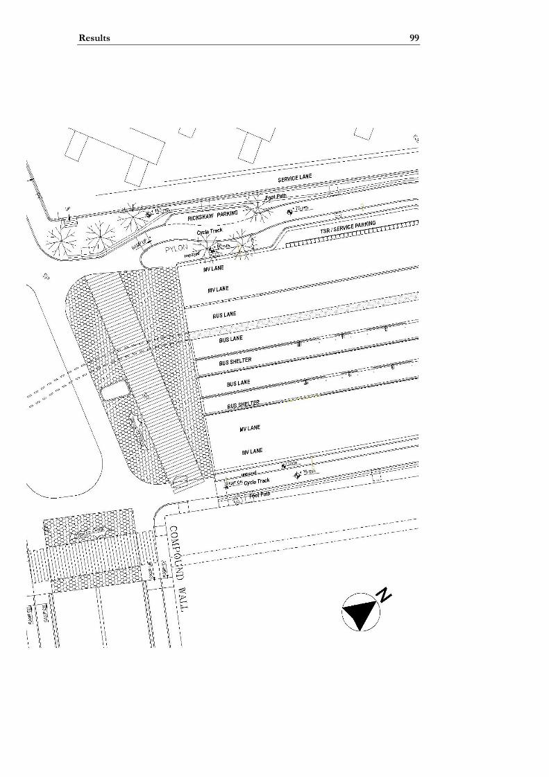
Results 99

100 Traffic Calming in Delhi
The use of cobble stone (change of pavement) and narrowing of lanes (by making physical separation between bus lanes and MV lanes) is in accordance with the principle of the Danish design rules. What is more interesting about the proposed layout, are the consequences of the bus lanes’ placement in the middle of the road. This will result in high demands of an effective signalization. Earlier it has been pointed out that red light violation at Orthonova today is a problem. Possible initiatives to reduce this problem are:
⎯ Prohibiting of left turn on red. By Elvik and Vaa (2004) it has been stressed, that permission to make left turn on red will increase the number of person injury crashes by up to 60 %.
⎯ Optimize the signal phases. Today the western leg and the eastern leg do not have green at the same time. This can lead to some confusion.
Another problem worth taking into consideration is large exposure that pedestrians will experience when bus stops are placed in the middle of the road. All pedestrians using the bus stop will have to cross motor traffic and thus leading to large exposure. If the bus stop was placed at the side of the road, not all pedestrians would have to cross motor traffic. Because the bus stop is part of the HCBS, it can be reasonable to make a comparison to tram systems also located in the middle of the road. In Gothenburg – which also was used as an example in chapter 1 – tram lines partially are located in the middle of the road. Studies have showed that 76 % of pedestrian-crashes in Gothenburg where trams are involved happen at, or near, a tram stop (Hedelin et al. 1996). Attention should be given to ensure that the pedestrian’s safety not is decreased in order to secure effective performance from the busses.
4.5 Proposed Layout at Dilli Haat In the view of the previous findings, a proposed layout at Dilli Haat is made. Figure 4.11 shows the base plan sketch. The proposal is not taking notice of the plans of a metro station on the west-side of the road. The underlying thought is about combining different measures of traffic calming, and thus not just be dependent of one measure to influence the road users. The challenge is to combine the measures in a way that will not lower the capacity or slow down the motor traffic at times without crossing pedestrians. A solution with a change in the pavement is suggested. The solution is aiming at increasing the feeling of safety as well as increasing the awareness of the location of the pedestrian crossing. The solution can be supplemented with measures like prior notice (signs) and/or special lighting at the crossing. The combination of prior notice and a sort of gateway at the crossing will be a large change with respect to the present design. Today, no information about the zebra crossing is given to the motor vehicles until they reach to the painted zebra marking.

Results 101
It is expected that the proposed counter measures at Dilli Haat will give more awareness about the location of the pedestrian crossing. Thus, conflicts where motor vehicles are unaware of the crossing until the last moment can be avoided. It is however more uncertain how the proposed redesign will effect the hierarchy among the road users. It was observed how motor vehicles even at low speed not were willing to yield for pedestrians who wanted to cross. It is estimated that the redesign will give more attention to the pedestrian’s formal right of way and less attention to who is biggest and strongest. In an attempt to help this change a so called “traffic squat” could be used. A traffic squat can be compared with a school safety patrol which it is known from the Nordic countries. At one of the big signalized intersections in Delhi – called ITO – a traffic squat in action was observed. The squat – four persons for a big intersection – helped all kind of road users to follow the traffic rules. This could be telling pedestrians to wait for the green light, walk on the zebra marking and remind car drivers to stop behind the yield line. Something similar could be done at Dilli Haat.
Figure 4.11: Base plan sketch of Dilli Haat. The north arrow is for guidance only.

102 Traffic Calming in Delhi
4.6 Prognosis of Countermeasures According to chapter 1, the main problem is related to a prognosis of countermeasures that describes and discusses provisions, modifications and estimated effects. The prognosis will comprise measures from the Danish design rules about traffic calming and their implementation in traffic environment in Delhi. Below, different measures will be listed. Not all the 14 types of measures from the Danish design rules will be involved. Instead 8 general types and their estimated effects are presented.
Location Adaptations / description Estimated effects in Delhi Prior Notice Arterial roads and local roads at all speeds and traffic intensities.
As a visual measure like signs, lighting and plantation……
Alone, no serious effect is expected.
Gateways Arterial roads and local roads at all speeds and traffic intensities.
Will often mark the change from a rural area to an urban area or from one speed limit to another. It is of great importance that the materials used are conspicuous.
British studies have proven a speed reduction by up to 10 km/h for developing countries (Quimby et al. 2003). A similar reduction is expectable in Delhi.
Humps Arterial roads and local roads at 50 km/h or below and at all traffic intensities.
Delhi Traffic Police recommends two types of humps with a preferred crossing speed at 25 km/h. It is estimated that the preferred crossing speed must be lower than the speed limit, for the hump to have an effect. However, design rules that include humps with more crossing speeds are prudent.
Best results are achieved when humps are laid as a series or being used in combination with other measures. Danish studies have proven a speed reduction by up to 10 km/h. The number of person injuries has been reduced between 38 % and 80 %. The number of all crashes has been reduced between 50 % and 71 %. (Danish Road Directorate 2004b) The effects in Delhi are expected to be slightly lower.

Results 103
Location Adaptations / description Estimated effects Elevated surface Arterial roads and local roads at 50 km/h or below and at all traffic intensities.
Can be combined with pedestrian crossings but can not be recommended for a whole intersection.
Elevated surfaces are estimated to have a good speed reducing effect (Danish Road Directorate 2006). An increase in crashes must be expected if used in a whole intersection (Elvik and Vaa 2004). Danish studies have proven a speed reduction by up to 10 km/h. The effects in Delhi are expected to be slightly lower.
Staggering Arterial roads and local roads at all speeds and traffic intensities.
This type of measure will have less effect on MTWs. To achieve a better effect it can be combined with gateways.
The best effect is achieved in combination with other measures. Because the effect on MTWs is expected to be low, the general effect is also expected to be low if used alone as a single measure.
Narrowing Arterial roads and local roads at 50 km/h or below and at all traffic intensities.
As above As above
Roundabout Arterial roads and local roads at all speeds and traffic intensities.
Has a speed reducing effect on all road users if the lateral displacement is big enough also to affect MTWs.
The number of person injuries can be reduced between 27 % and 35 % if intersections are change into roundabouts. The number of material injuries will increase with up to 52 %. (Elvik and Vaa 2004) The effects in Delhi are expected to be slightly lower.

104 Traffic Calming in Delhi
Location Adaptations / description Estimated effects Combinations Combinations of the above mentioned measures can be used at a single site, over a stretch or in a whole area.
By using the same design over a large area the road users “learn” how to move about with the new measures in the environment. Recognisability is an important key word.
In Gothenburg, Sweden, a reduction of 17 % of police reported injuries and 27 % hospital reported injuries were achieved. 75 % of the decrease is estimated to be a direct consequence of traffic calming measures. (Thulin and Nilsson 2004) A meta-analysis of 33 existing traffic calming schemes proved a reduction in number of crashes by 15-20 % (area wide implementation), 8-15 % (arterial roads) and 25-55 % (local roads). (Elvik 2001) The effects in Delhi are expected to be slightly lower. It is in addition estimated that effects from the above measures will be minimal if not used in combinations or in series.

Chapter 5
Epilogue
Through a discussion the conclusions will be set up. Afterwards, a perspective on the given study in Delhi is given plus suggestions to further studies.
5.1 Discussion The analysis of the conflict data was in reality a “three dimensional” analysis, but made in two separate stages: first CDBase and second the subjective severity scale. The analysis with CDBase is two dimensional (speed and TA) while the third dimension is the subjective estimated severity. Figure 5.1 illustrates this. The analysis showed that the “severity-dimension” did not change the result from the “two dimensional” analysis. Still it is interesting whether speed and the TA-value can be supplemented with a third factor and thus make the method more flexible. It is estimated that severity still is the best supplement to speed and the TA-value.
As part of the description of a serious conflict the words “undesired phenomena” is used. This is not a part of the definition of a conflict, but it is included in the subjective severity scale used in the study in Delhi (see chapter 2). It is, however, estimated that this wording not is suitable in Delhi. Some types of risky situations are accepted by the Delhi pedestrians to be able to cross the streets at all and some of the risky situations may also be undesired but still accepted. Risky situations are accepted both in
TA
Spe
ed
Seve
rity
Figure 5.1: In reality a 3-dimensional analysis of the conflict data has been made.
106 Traffic Calming in Delhi
India and in the Nordic countries. It is however estimated that a larger amount of the accepted risky situations also is undesired in the Nordic countries than in India. The wording “Undesired phenomena” should not be given great weight when doing the observations. In the worst case, it could mean that all conflicts – except those extremely severe – would be considered part of the normal and accepted risk by the local road user, and thus not be recorded as a conflict by the observer. The wording “undesired phenomena” is therefore not a part of the suggestion for a new subjective severity scale given in chapter 4.
The physical design at Orthonova and Dilli Haat are very different from each other. At Dilli Haat it can be discussed if traffic calming is the most appropriate solution. Separation of different types of road users is another possibility. Footbridges across Aurobindo Marg, or tunnels under, can be found north and south of Dilli Haat. The most visible problem with for instance a footbridge is the construction prize. Another problem is – if the pedestrians are spread over a large area, like at Dilli Haat – that many of the users will have to make a detour to use it. Pedestrians always will go for the shortest possible way. Thus traffic calming still should be considered as a part of the solution, possibly combined with separation.
Indian pedestrians accept that they are the weak part in the hierarchy. When doing this, they also ignore some of the formal rules, e.g. that pedestrians have the right of way at zebra crossings. This is different from the Nordic countries. Here, pedestrians are more focused on their right of way at zebra crossings. This can result in “uncontrolled” conflicts because pedestrians walk onto the zebra marking in the belief that the cars will yield. –High risk perception in spite of low risk willingness and high feeling of safety. The Indian pedestrian’s low rank in the hierarchy leads to high risk perception, it can be argued. The Indian pedestrians generally have high risk willingness and low feeling of safety. To ensure low risk perception in spite of high risk willingness, measures of traffic calming can be used. If the hierarchy, in this way, becomes less widespread, it will be of benefit to the pedestrians. The use of traffic calming measures can not eliminate the hierarchy among the road users but it is estimated that it can be a helpful measure to give awareness of e.g. pedestrians’ formal rights.
It has been argued for that speed breakers have to be “in bad conditions, just like the rest of the road network” in order to be effective. This should, however, not be implemented by poor construction work, but instead by a preferred crossing speed lower than the speed limit. It is important not to see this as an eternal regulation. As the condition of the whole network improves, the humps gradually, and in phases, must be replaced, with the view of having similarity between preferred crossing speed and the relevant speed limit. To get to this point, a standard of hump design must
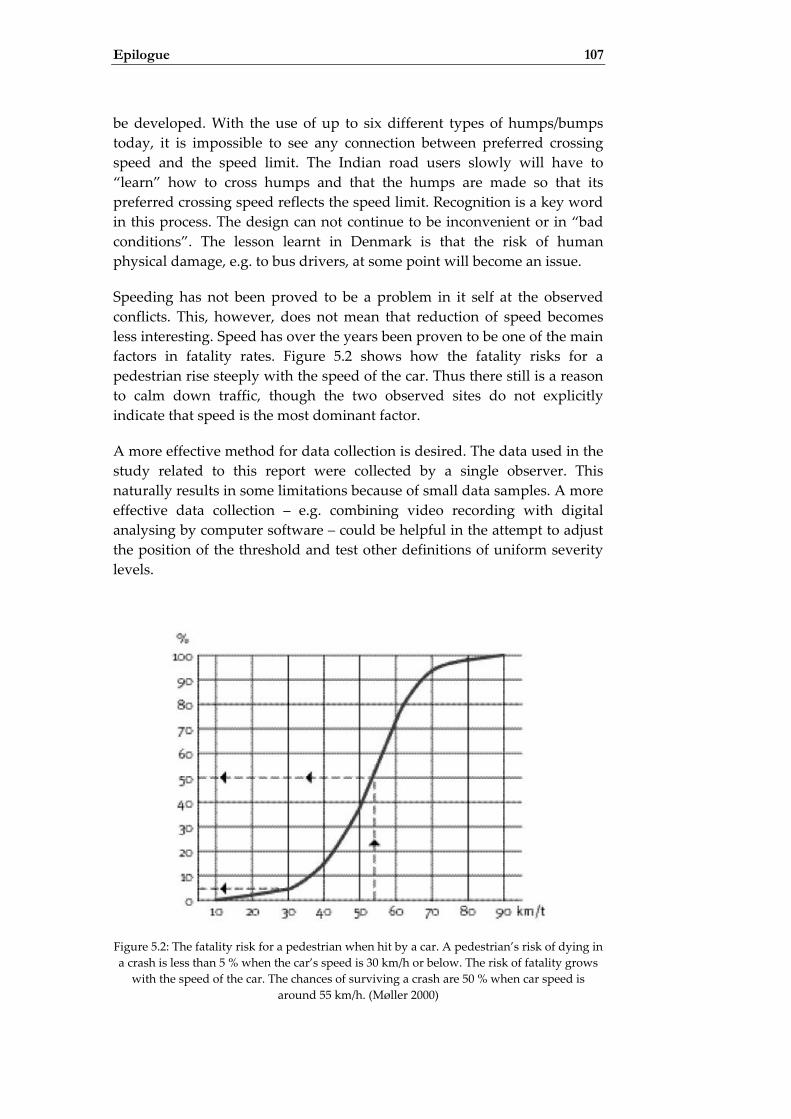
Epilogue 107
be developed. With the use of up to six different types of humps/bumps today, it is impossible to see any connection between preferred crossing speed and the speed limit. The Indian road users slowly will have to “learn” how to cross humps and that the humps are made so that its preferred crossing speed reflects the speed limit. Recognition is a key word in this process. The design can not continue to be inconvenient or in “bad conditions”. The lesson learnt in Denmark is that the risk of human physical damage, e.g. to bus drivers, at some point will become an issue.
Speeding has not been proved to be a problem in it self at the observed conflicts. This, however, does not mean that reduction of speed becomes less interesting. Speed has over the years been proven to be one of the main factors in fatality rates. Figure 5.2 shows how the fatality risks for a pedestrian rise steeply with the speed of the car. Thus there still is a reason to calm down traffic, though the two observed sites do not explicitly indicate that speed is the most dominant factor.
A more effective method for data collection is desired. The data used in the study related to this report were collected by a single observer. This naturally results in some limitations because of small data samples. A more effective data collection – e.g. combining video recording with digital analysing by computer software – could be helpful in the attempt to adjust the position of the threshold and test other definitions of uniform severity levels.
Figure 5.2: The fatality risk for a pedestrian when hit by a car. A pedestrian’s risk of dying in a crash is less than 5 % when the car’s speed is 30 km/h or below. The risk of fatality grows
with the speed of the car. The chances of surviving a crash are 50 % when car speed is around 55 km/h. (Møller 2000)

108 Traffic Calming in Delhi
5.2 Conclusions Hypothesis 1:
⎯ The Swedish traffic conflict technique is usable in the mixed traffic composition in Delhi to give diagnoses to traffic problems.
⎯ It has not been proven that a subjective severity scale is necessary in addition to the original discrimination between serious- and non-serious conflicts. Instead it is estimated that a subjective severity scale is a good supplement to the results from CDBase.
⎯ A suggestion for a new subjective severity scale has been made in chapter 4.
⎯ It has not been proven that the threshold between serious- and non-serious conflicts should be given another position in the speed-TA graph.
Hypothesis 2:
⎯ The facilities for pedestrians are often inadequate or simply non-existing.
⎯ A combination of measures from the Danish design rules of traffic calming is estimated to give a speed reducing effect in the mixed traffic composition in Delhi.
A prognosis of traffic safety measures is drawn up in the previous chapter. It is build upon the measures from the Danish design rules of traffic calming and with the aim of being used in the mixed traffic in Delhi.
5.3 Perspective This section comprises a discussion on how the study was planned, carried out and analysed.
The planning started in February 2006 with correspondence by e-mail with CUTS and IIT. It did not take long before a distribution became clear: CUTS was to help with accommodation and practical information while IIT was to help with academic and professional information. Before the study visit could begin, the following tasks were to be made: Time schedule, hypotheses and planning of each of the studies. Departure to Delhi was at 20 April 2006.
The first week in Delhi was reserved to acclimatisation, selection of traffic sites for observations and adapting the planned work. Especially the last part was advantageous. During the first week the hypotheses and time schedule continuously were fine-tuned. The complete time schedule for the observations is showed in appendix C. Because of the high temperatures – around 40 degrees Celsius at noon – the conflict observations were changed from six hours per day to four hours per day.

Epilogue 109
The planned study only involved one single observer. Thus no problems with training an observer team were part of the tasks. Another challenging task however was to get used to the general traffic situation and – not least - to get used to the conflict situations. With an understanding of traffic based on the environment in the Nordic countries, the first two days of conflict studies was challenging. -Maybe a test study would have been advantageous. Departure from Delhi was at 5 June 2006.
The analysis and publication of results spanned two and a half month.
5.4 Further studies This section gives suggestions to further studies in Delhi.
5.4.1 Bicycle tracks in Delhi Only a very little number of bicycle tracks exist in Delhi. This is probably to change over the coming years. No master plan for bicycle tracks exists. A clarification of the needs and scope that is necessary would be of great interest. If police reports are accessible, the nature of bicycle crashes can be described. This can lead to a discussion about the location of bicycle crashes. –Mainly between two categories: stretches or intersections. A comparison can be made with the Nordic countries. The results can lead to definitions of the design of bicycle tracks that will be most effective in Delhi. This can e.g. deal with road types where bicycle tracks should be implemented and the design around intersections.
5.4.2 Comparison of willingness of risk Ongoing studies at TRIPP concern the willingness of risk among crossing pedestrians. This involves observations and analyses of crossing pedestrians’ waiting time and their acceptance of time gaps between motor vehicles. The relationship between the velocity of the motor vehicle and the time gap can be used as a measure of the risk willingness. Studies comparing Indian pedestrians and European pedestrians could help illustrate the difference between road users.
Data collection and analyses are already ongoing at TRIPP. Data collection would have to be made in the Nordic countries. Behavioural studies of crossing pedestrians at traffic sites without signal regulation is suggested. The selection of specific traffic sites has to be made in association with the chosen Indian traffic sites. From the Nordic traffic sites, the velocity of the motor vehicles, pedestrians’ waiting time and their accepted time gaps between motor vehicles would have to be analysed from video recordings.
5.4.3 Public Transportation Together with the TSRs, the bus companies are very important for the daily public transport in Delhi. During the daytime it is normal if busses are

110 Traffic Calming in Delhi
overcrowded. Public transportation will continue to have an important role in Delhi in many years to come because of the big low- and middle income class that cannot afford to have a car or a MTW. Thus it will be interesting to work with an optimization of the bus system. This can be with regard to effective route planning and the safety of the occupants. Risky behaviour of bus drivers and improvements of bus design are also issues that could be aim for an analysis.
If access to police records is possible, studies of crash locations between busses and pedestrians can be studied. This can lead to a definition of a safe design of bus stops.
5.4.4 TCT studies A new traffic conflict study involving a larger data range and more traffic sites, possibly in a number of different cities would be interesting. With a larger data range, more clear defined results possibly could be achieved. Another issue of the study would be to identify the advantages of using traffic conflict technique in countries where the accessible crash reports are imperfect. If police records are accessible, the study can involve studying a correlation between serious conflicts and injury crashes.

References
Amundsen, F. H. and Hyden, C. (1977) Proceedings of The First Workshop on Traffic conflicts, Oslo. TTI, Oslo, Norway and LTH Lund, Sweden.
Danish Road Directorate (2004a) Katalog over typegodkendte bump, September 2002, Revideret januar 2004, Vejdirektoratet – Vejregelrådet, København, ISBN 87-7923-386-4.
Danish Road Directorate (2004b) Erfaringsopsamling om trafiksanering med hastighedsdæmpning, Vejbump, Vejdirektoratet – Vejstandardafdelingen, København.
Danish Road Directorate (2006) Byernes trafikarealer, Hæfte 7, Fartdæmpning, Vejdirektoratet - Vejregelrådet, http://www.vejregler.dk/pls/vrdad/vr_layout.vis?p_gren_id=3447, visited 23 May 2006.
Delhi Traffic Police (2004) Road Accidents in Delhi 2004, Delhi Traffic Police, Delhi.
Delhi Traffic Police (2006a) http://www.delhitrafficpolice.nic.in/speed-breaker.htm, visited 4 August 2006.
Delhi Traffic Police (2006b) http://www.delhitrafficpolice.nic.in/road-marking.htm, visited 4 August 2006.
Delhi Traffic Police (2006c) http://www.delhitrafficpolice.nic.in/speed-limitation.htm, visited 4 August 2006.
Eicher (2006) Delhi City Map, 2nd edition, Eicher Good Earth Limited, New Delhi, ISBN 81-900601-7-1.
Elvik, R. (2001) Area-wide Traffic Calming Schemes: a Meta-Analysis of Safety effects, Accident Analysis and Prevention, Vol. 33, No. 3, pp. 327-336.

112 Traffic Calming in Delhi
Elvik, R., Vaa, T. (2004) The Handbook of Road Safety Measures, Institute of Transport Economics, Norwegian Centre for Transport Research, Olso, First edition, ISBN 0-08-044091-6.
GoogleEarth (2006) Software provided for free at http://www.earth.google.com, maps downloaded 9 July 2006.
Hedelin, A., Björnstig, U., Brismar, B. (1996) Trams – a Risk Factor for Pedestrians, Accident Analysis and Prevention, Vol. 28, No. 6, pp. 733-738.
Hyden, C. (1987) The Development of a Method for traffic safety evaluation: The Swedish Traffic Conflict Technique, Lund Institute of Technology, Department of Traffic Planning and Engineering, Lund, Sweden.
IRTAD (2006) International Road Traffic and Accident Database, http://www.bast.de/htdocs/fachthemen/irtad/english/grafics.htm, visited 15 June 2006.
Kjemtrup, K., Herrstedt, L. (1992) Speed Management and Traffic Calming in Urban Areas in Europe: a Historical View, Accident Analysis and Prevention, Vol. 24, No. 1, pp. 57-65.
Kopits, E., Cropper, M. (2005) Traffic fatalities and economic growth, Accident Analysis and Prevention, Vol. 37, No. 1, pp. 169-178.
Maps of India (2006) www.mapsofindia.com, visited 6 July 2006.
Mohan, D., Bawa, P. S. (1985) An Analysis of Traffic Fatalities in Delhi, India, Accident Analysis and Prevention, Vol. 17, No. 1, pp. 33-45.
Mohan, D., Tiwari, G. (1998) Traffic Safety in Low-Income Countries: Issues and Concerns Regarding Technology Transfer from High-Income Countries, In: Reflections of the transfer of traffic safety knowledge to motorising nations, Melbourne, Global Traffic Safety Trust, 27-56.
Mohan, D. (2002) Traffic safety and health in Indian cities, Journal of Transport and Infrastructure, Vol. 9, No. 1, pp. 79-93.
Mohan, D. (2004) The Road Ahead – Traffic Injuries and Fatalities in India, Transportation Research and Injury Prevention Program, WHO and Indian Institute of Technology Delhi.
Muhlrad, N. (2005) Traffic Conflict Technique: Some Data to Supplement Accident Analysis, In: The Way Forward, Transportation Planning

References 113
and Road Safety, Macmillan India Ltd., New Delhi, ISBN 1403 92502 X
Murray, C. J. L., Lopez, A. D. (1996) The Global Burden of Disease: a Comprehensive assessment of mortality and disability from diseases, and risk factors in 1990 and projected to 2020, Boston, MA, Harvard School of Public Health.
Møller, H. A. (2000) Hver ulykke er én for meget – Trafiksikkerhed starter med dig, Mod nye mål 2001-2012, Færdselssikkerhedskommis-sionen, Trafikministeriet, Copenhagen, Denmark, ISBN 87-90262-81-6.
Peden, M., Scurfield, R., Sleet, D. et al. (2004) World report on road traffic injury prevention, World Heath Organization, Geneva, ISBN 92 4 156260 9.
Quimby, A., Hills, B., Baguley, C., Fletcher, J. (2003) Urban Safety Management: Guidelines for Developing Countries, Transport Research Laboratory.
Rosbach, O., Wellis, W., Jørgensen, L., Mertner, J. (1996) Miljøprioriterede gennemfarter – Effekter i 21 byer, Vejdirektoratet, København, ISBN 87-7491-767-6
Ross, A., Baguley, C., Hills, B. et al. (1994) Towards Safer Roads in Developing Countries – a Guide for Planners and Engineers, Transport Research Laboratory.
Shbeeb, L. (2000) Development of a traffic conflict technique for different environments. A comparative study of pedestrians conflicts in Sweden and Jordan, Lund, Lund Institute of Technology, Bulletin 188.
Statens Vegvesen (2006) The Norwegian Directorate of Public Roads, http://www.vegvesen.no/horinger/hb_072/Del5_Kombi_fysiske_fartsdemp_tiltak.pdf, visited 16 August 2006.
Söderlund, N., Zwi, A. B. (1995) Traffic-related mortality in industrialized and less developed countries, Bulletin of the World Health Organization, 73: 175-182.
Thulin, H., Nilsson, G. (2004) Trafiksäkerhetsutveckling i Göteborg, Väg- och transportforskningsinstitutet, Linköping, ISSN 0347-6049
Tingvall, C. (1997) The Zero Vision. A road transport system free from serious health losses. In: Holst von, H., Nygren, Å., Thord, R. (Eds.),
114 Traffic Calming in Delhi
Transportation, Traffic Safety and Health. Springer Verlag, Berlin, pp. 37-57.
Tiwari, G., Mohan, D., Fazio, J. (1998) Conflict Analysis for Prediction of Fatal Crash Locations in Mixed Traffic Streams, Accident Analysis and Prevention, Vol. 30, No. 2, pp. 207-215.
Tiwari, G., Mohan, D., Muhlrad, N. (2005) The Way Forward – Transportation Planning and Road Safety, Macmillan India Ltd., New Delhi, ISBN 1403 92502 X
Transport- og Energiministeriet (2006) Mere trafiksikkerhed på vejene, Transport- og Energiministeriet, København, ISBN 87-91511-60-7
Wellis, W., Greibe, P., Andersson, P. K. et al (2003) 21 miljøprioriterede bygennemfarter – den trafiksikkerhedsmæssige effekt, Rapport nr. 281, Vejdirektoratet, København, ISBN 87-7923-619-7

Appendix A
Signal Plan for Orthonova
Two signal plans for Orthonova is presented in this appendix. The first is the plan that was provided by the Delhi Traffic Police through TRIPP. The second is the plan that was observed during field studies.
A.1 Delhi Traffic Police Through TRIP the following information in Table A.1 to Table A.4 was provided.
Table A.1: Week plan that says which day plan that is followed on which day.
Day Mon Tue Wed Thu Fri Sat Sun Day Plan 1 1 1 1 1 1 2
Table A.2: Overview of the two different day plans that is in use at Orthonova
Cycle From To Day Plan 1 3 23:00 06:00 2 06:00 09:00 1 09:00 11:00 2 11:00 17:00 1 17:00 20:00 2 20:00 23:00 Day Plan 2 3 23:00 06:00 2 06:00 23:00
Table A.3: Plan of the five different phases according to the three different cycles
Phase Cycle 1 2 3 1 20 20 15 2 45 35 25 3 25 20 15 4 20 15 15 5 20 15 15 Cycle Time 130 105 85

116 Traffic Calming in Delhi
Table A.4: The alphanumeric code connected to each phase refers to Figure A.1 and which signal post that has green light.
Phase 1 Phase 2 Phase 3 Phase 4 Phase 5 A1, A1r A1, A2 A2, A2r B1 B2
A1A2
r
A2A1
r
B1
B2
A2rA2
A1r
A1
B2
B1
Shas
tri Ma
rg
Shas
tri Ma
rg
Figure A.1: Signal plan of Orthonova
A.1 Own observations During field studies the following phases showed in Figure A.2 were observed in the peak hour between 7 and 8 pm. Note that the number of phases matches with the above, but the phase times do not.

Appendix 117
Figure A.2: Signal cycle for Orthonova observed during the making of field studies. The time values are in seconds. The alphanumeric codes refer to Figure A.1.

118 Traffic Calming in Delhi

Appendix 119
Appendix B
Traffic Conflict Recording Form
On the next page a full size example of the pre-arrange traffic conflict technique recording form from Lund University - that was used in the field studies - is showed.


Appendix 121
Appendix C
Schedule for Field studies
The next two pages show the schedule that was followed during the field studies in Delhi in May and June 2006, see Figure C.1. Note that the schedule is spreading over two pages and that one row represents one week. Due to illness – marked with blue colour - in the second week of observations the rest of the schedule was afterwards fitted to the new period of time available. Note in addition that a change in the observation time in the morning was made in the third week. This change was made in order to overlap less with the morning peak hour – from 9 to 10 am – and thus be able to observe more free vehicles at running speed.

122 Traffic Calming in Delhi
Figure C.1: Schedule for fields studies -

Appendix 123
- in Delhi, May/June 2006.

124 Traffic Calming in Delhi

Appendix 125
Appendix D
Traffic Counts at Orthonova
The next two pages will show data - provided by the Delhi Traffic Police through TRIPP – containing one-hour traffic counts from Orthonova in the morning peak hour (9 to 10 am) and in the evening peak hour (7 to 8 pm). The diagrams contain no information about orientation except for area names. The diagrams are so to say up side down when the pages are read at landscape orientation; Chirac Delhi is north of the intersection, Dakshin Puri is east of the intersection, etc.


128 Traffic Calming in Delhi

Appendix 129
Appendix E
Traffic Counts at Dilli Haat
Wednesday 24 May 2006 the following counts were made. A five minute count was made for each of the following road groups, which summarized all together spread over one hour when two directions are counted independently: Car, MTW, TSR, bus/truck, bicycle, pedestrian. First cars was counted in both directions, then MTW in both directions, etc – following the before mentioned order.
E.1 Morning Peak Hour Between 9 and 10 am on Wednesday 24 May 2006 the morning peak hour count was made. See Table E.1 and Table E.2.
Table E.1: Five minute traffic counts in the morning peak hour in both directions at Dilli Haat. Multiplied to represent one hour of traffic and the AADT.
Towards South Towards North Road User 5 min 1 hour AADT 5 min 1 hour AADT Cars 144 1728 17280 202 2424 24240 MTWs 143 1716 17160 114 1368 13680 TSRs 77 924 9240 59 708 7080 Busses/Trucks 23 276 2760 20 240 2400 Bicycles 5 60 600 2 24 240
Table E.2: Five minute traffic counts in the morning peak hour of pedestrians at Dilli Haat. Multiplied to represent one hour of traffic and the AADT.
Road User 5 min 1 hour AADT Pedestrians towards west (Dilli Haat crafts market) 26 312 3120 Pedestrians towards east (INA market) 44 528 5280

130 Traffic Calming in Delhi
E.2 Evening Peak Hour Between 7 and 8 pm on Wednesday 24 May 2006 the evening peak hour count was made. See Table E.3 and Table E.4.
Table E.3: Five minute traffic counts in the evening peak hour in both directions at Dilli Haat. Multiplied to represent one hour of traffic and the AADT.
Towards South Towards North Road User 5 min 1 hour AADT 5 min 1 hour AADT Cars 142 1704 17040 152 1824 18240 MTWs 56 672 6720 89 1068 10680 TSRs 50 600 6000 48 576 5760 Busses/Trucks 9 108 1080 17 204 2040 Bicycles 6 72 720 5 60 600
Table E.4: Five minute traffic counts in the evening peak hour of pedestrians at Dilli Haat. Multiplied to represent one hour of traffic and the AADT.
Road User 5 min 1 hour AADT Pedestrians towards west (Dilli Haat crafts market) 16 192 1920 Pedestrians towards east (INA market) 46 552 5520

Appendix 131
Appendix F
Speed Measurements at Orthonova
The data in Table F.1 have been provided by TRIPP and is a part of the project of designing the HCBS. The values are split up into journey speed and running speed:
⎯ Journey speed represents vehicles free of disturbing factors such as other road users.
⎯ Running speed represents vehicles that run in a line and most likely have adapted their speed hereafter.
The values are further split up into general traffic and public traffic:
⎯ General traffic represents a broad mix of the traffic at the intersection. ⎯ Public transport represents the different types of busses from
different bus companies that operate in the intersection.
Table F.1: Average speed in the intersection of Orthonova for general traffic and public transport at journey speed and running speed.
Journey Speed Running Speed General traffic 20-30 20-30 Public transport 10-20 20-30

132 Traffic Calming in Delhi

Appendix 133
Appendix G
Speed Measurements at Dilli Haat
On Wednesday 31 June 2006 the data in Table G.1 was collected. A hand held “speed gun” – which uses the reflection of a laser bean to calculate the speed – was used. The values are split up into journey speed and running speed:
⎯ Journey speed represents vehicles free of disturbing factors such as other road users. The following definition was used during the measuring: the vehicle that is being measured must have at least two other vehicles in front of it within the next 100 meters.
⎯ Running speed represents vehicles that run in a line and most likely have adapted their speed hereafter. The following definition was used during the measuring: the vehicle that is being measured must have at least 100 meters of free space in front of it.
The measurements were made just before the peak hour. At that time there are both free vehicle and vehicles running in a line. Thus it is possible to measure both journey speed and running speed. Towards north the measuring was made between 5 and 7 pm while the measuring towards south was made between 8 and 9 am.
Note that the table spreads over three pages.
Table G.1: Journey speed and running speed observed for both directions at Dilli Haat for the peak hours. The measurements were made on a Wednesday.
Towards North (between 5 and 7 pm)
Towards South (between 8 and 9 am)
Journey Speed Running Speed Journey Speed Running Speed Obs. No. [km/h] [km/h] [km/h] [km/h] 1 37 40 48 45 35 45 39 58 28 38 36 68 35 38 57 58 5 38 33 43 48 26 48 43 68
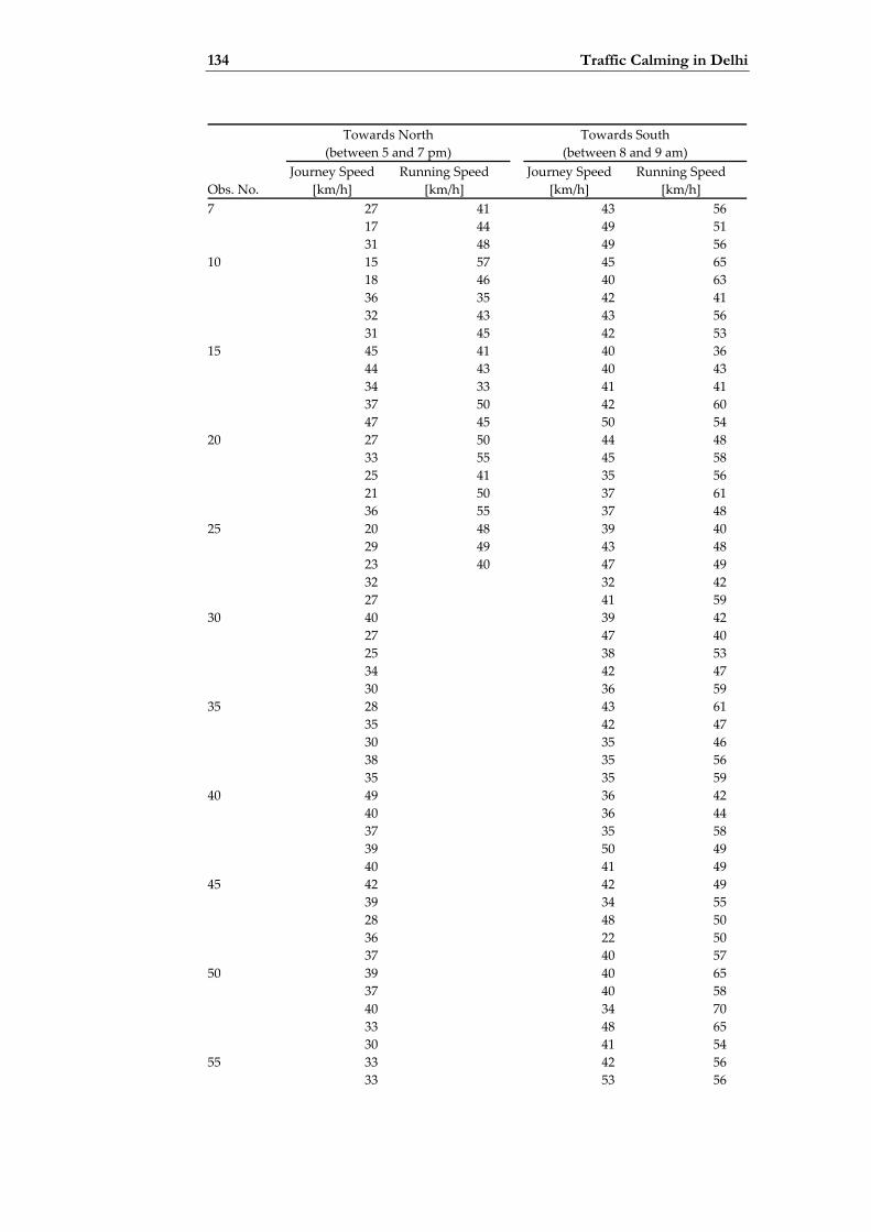
134 Traffic Calming in Delhi
Towards North (between 5 and 7 pm)
Towards South (between 8 and 9 am)
Journey Speed Running Speed Journey Speed Running Speed Obs. No. [km/h] [km/h] [km/h] [km/h] 7 27 41 43 56 17 44 49 51 31 48 49 56 10 15 57 45 65 18 46 40 63 36 35 42 41 32 43 43 56 31 45 42 53 15 45 41 40 36 44 43 40 43 34 33 41 41 37 50 42 60 47 45 50 54 20 27 50 44 48 33 55 45 58 25 41 35 56 21 50 37 61 36 55 37 48 25 20 48 39 40 29 49 43 48 23 40 47 49 32 32 42 27 41 59 30 40 39 42 27 47 40 25 38 53 34 42 47 30 36 59 35 28 43 61 35 42 47 30 35 46 38 35 56 35 35 59 40 49 36 42 40 36 44 37 35 58 39 50 49 40 41 49 45 42 42 49 39 34 55 28 48 50 36 22 50 37 40 57 50 39 40 65 37 40 58 40 34 70 33 48 65 30 41 54 55 33 42 56 33 53 56

Appendix 135
Towards North (between 5 and 7 pm)
Towards South (between 8 and 9 am)
Journey Speed Running Speed Journey Speed Running Speed Obs. No. [km/h] [km/h] [km/h] [km/h] 57 28 44 51 29 44 49 32 19 56 60 37 45 56 30 44 52 35 20 44 31 45 56 35 44 67 65 34 19 51 24 45 45 35 32 48 38 32 44 36 32 42 70 33 36 49 39 37 58 39 45 44 35 26 62 25 25 52 75 29 39 49 28 47 52 22 40 49 36 48 52 22 43 60 80 26 39 48 27 33 49 30 38 44 27 34 62 26 45 45 85 25 32 45 20 32 35 27 40 57 22 40 43 33 27 54 90 25 28 58 30 21 54 27 28 67 32 27 53 29 30 56 95 25 33 52 33 34 48 41 25 55 36 41 65 36 36 53 100 41 35 60 Average 32 44 39 53

136 Traffic Calming in Delhi

Appendix 137
Appendix H
Example of Conflict Recording Form
The next two pages show two examples of a conflict recording form from Orthonova and Dilli Haat respectively.