HAL Id: hal-01242492https://hal.archives-ouvertes.fr/hal-01242492

Submitted on 12 Dec 2015

HAL is a multi-disciplinary open accessarchive for the deposit and dissemination of sci-entific research documents, whether they are pub-lished or not. The documents may come fromteaching and research institutions in France orabroad, or from public or private research centers.

L’archive ouverte pluridisciplinaire HAL, estdestinée au dépôt et à la diffusion de documentsscientifiques de niveau recherche, publiés ou non,émanant des établissements d’enseignement et derecherche français ou étrangers, des laboratoirespublics ou privés.

Traffic-Aware Training and Scheduling for MISOWireless Downlink Systems

Apostolos Destounis, Mohamad Assaad, Mérouane Debbah, Bessem Sayadi

To cite this version:Apostolos Destounis, Mohamad Assaad, Mérouane Debbah, Bessem Sayadi. Traffic-Aware Train-ing and Scheduling for MISO Wireless Downlink Systems. IEEE Transactions on Informa-tion Theory, Institute of Electrical and Electronics Engineers, 2015, 61 (5), pp.2574 -2599.<10.1109/TIT.2015.2411607>. <hal-01242492>

1

Traffic-Aware Training and Scheduling for

MISO Wireless Downlink SystemsApostolos Destounis, Member, IEEE, Mohamad Assaad, Member, IEEE, Merouane Debbah,

Fellow, IEEE, and Bessem Sayadi, Member, IEEE

Abstract

In this paper, the problem of feedback and active user selection in MISO wireless systems such

that the system’s stability region is as big as possible is examined. The focus is on a system in a

Rayleigh fading environment where zero forcing precoding is used to serve all active users in every slot.

Acquisition of the channel states is done via uplink training in Time Division Duplexing mode by the

active users. Clearly, only a subset of users can perform uplink training and the selection of this subset

is a challenging and interesting problem especially in MISO systems. The stability regions of a baseline

centralized scheme and two novel decentralized policies are examined analytically. In the decentralized

schemes, the transmitter broadcasts periodically the queue state information and the users contend for the

channel in a CSMA-based manner with parameters based on the outdated queue state information and

real-time channel state information. We show that, using infrequent signaling between the base station

and the users, the decentralized policies outperform the centralized policy. In addition a threshold-based

user selection and training scheme for discrete-time contention is proposed. The results of this work

imply that, as far as stability is concerned , the users must be involved in the active user selection and

feedback/training decision. This should be leveraged in future communication systems.

A. Destounis is with CentraleSupelec, 3 rue Joliot-Curie, 91192, Gif-sur-Yvette, cedex.

France.(apostolos.destounis@supelec.fr).

M. Assaad is with Laboratoire des Signaux et Systemes (L2S, UMR CNRS 8506) CentraleSupelec , 3 rue Joliot-Curie, 91192,

Gif-sur-Yvette, cedex. France. (mohamad.assaad@supelec.fr)

M. Debbah is with CentraleSupelec, 3 rue Joliot-Curie, 91192, Gif-sur-Yvette, cedex. France. (merouane.debbah@supelec.fr)

B. Sayadi is with Alcatel-Lucent Bell Labs France, Villarceaux, Route de Villejust, 91620, Nozay, cedex. France

(bessem.sayadi@alcatel-lucent.com)

The work presented in this paper was done while the first author was with Alcatel-Lucent Bell Labs France. Parts of this

paper have been presented at the IEEE International Symposium on Information Theory (ISIT), Honolulu, HI, U.S.A., 2014 and

have been accepted for presentation at the IEEE International Conference on Communications (ICC), London, U.K., 2015.

2

Index Terms

MISO broadcast channel, stability, bursty traffic, zero forcing

I. INTRODUCTION

The use of multiple antennas [1] has emerged as one of the enabling technologies to increase the

performance of wireless systems. The ability to serve multiple users in the same time-frequency block

has made the use of multiple antennas at the base stations (BSs) particularly attractive for multiuser

downlink systems, and the benefits coming from this fact are well understood [2]. The decision to be

taken every timeslot then is (i) which users should be scheduled and (ii) how the corresponding signals

should be precoded.

From an information theoretic point of view, the capacity region of the multiple-input multiple-output

(MIMO) broadcast channel (BC) is well characterized [3], assuming perfect channel state information

at the transmitter. However, achieving this region requires Dirty Paper Coding, which is complex to

implement, while the assumptions of perfect channel state information and use of Gaussian codebooks

are strong in practical systems. Linear precoding schemes such as zero forcing (ZF) , a scheme that cancels

the interference among the scheduled users, are more desirable to use in practice. There are many works

on the issue of imperfect channel state information (CSI) , see for example [4] and references therein,

[5], [6], [7], however the focus is mainly on quantities like sum throughput and they do not take into

account the traffic processes of the users.

It is of theoretical and practical interest to study the impact of MIMO in the higher layers [8]. For the

MIMO media access control (MAC) , a precoding strategy that achieves the stability region is presented

in [9], under the assumptions of perfect CSI and use of Gaussian codebooks. This policy is based on

Lyapunov drift minimization given the queue lengths and channels every timeslot and makes use of

superposition coding and successive decoding. This is hard to implement in practice. Regarding the BC

(i.e.the downlink system), authors in [10] have proposed a technique based on ZF precoding, with a

heuristic user scheduling scheme that selects users whose channel states are nearly orthogonal vectors

and illustrate the stability region this policy achieves via simulations. Authors in [11] notice that the policy

resulting from the minimization of the drift of a quadratic Lyapunov function is to solve a weighted sum

rate maximization problem (with weights being the queue lengths) each timeslot and they propose an

iterative water-filling algorithm for this purpose. In addition, authors in [12] propose to use the delays

of the packets in the head of each queue along with the queue lengths as weights. All these works

3

assume accurate CSI available at the transmitter. In the case of delayed channel state information and

channels having a correlation in time, authors in [13] compare the stability and delay performance of

opportunistic beamforming and space time coding while in [14] they propose a user scheduling and

precoding algorithm. In addition, in [15], the authors study the impact of channel state quantization in

the stability of a system using ZF precoding under a centralized scheme where the transmitter selects the

users to be scheduled based only on the queue lengths. However, the fact that radio resources i.e. time

and/or spectrum are needed for the BS to acquire channel state information is not accounted for in these

works.

In this paper we consider a multiple-input single-output (MISO) downlink system where the BS acquires

CSI from the users in time-division duplexing (TDD) mode, in order to exploit the channel reciprocity.

There are two ways for this: (i) users estimate their channel and then feed back the CSI in a time-

division multiple access (TDMA) manner and (ii) users send (pre-assigned) training sequences in the

uplink so that the BS can estimate the channels (uplink and downlink channels are the same due to

reciprocity). The latter scheme is implemented using orthogonal sequences among the users, so that the

BS can decode every transmission without errors. Orthogonal sequences are produced e.g. by Walsh-

Hadamard on pseudonoise sequences, and their length should be proportional to the number of users

that simultaneously train in the uplink. Uplink training is considered the most promising for MIMO

systems, since the length of the training sequences does not depend on the number of antennas at the BS

. However, due to the orthogonality requirement, their length is proportional to the number of users that

perform uplink training 1. That means that in a system with many users, not all users should be selected to

train at the same time, therefore the users that should train at every slot must also be selected. The TDD

system model with uplink training has been also examined in [16], however they do not take into account

that last observation, that is not all users should participate in the training at every slot. In this paper

we focus on the tradeoff between having many users training (so having data transmitted to many users

simultaneously) and having much time of the slot devoted to data transmission (which means having few

users train). In order to simplify things, we focus on ZF precoding used at the transmitter. This scheme is

widely used in the literature because it is simple to implement while capturing the fundamental tradeoffs

arising from using multiple antennas and performing well in some scenarios of interest (e.g. in systems

with many users [17] and/or with BSs with large antenna arrays). In addition, we will assume that all

1In the case where CSI acquisition is done by feedback in TDMA manner, then the time needed for CSI acquisition is also

proportional to the number users that feed back.

4

users that perform uplink training in a slot get scheduled. This is an assumption used fairly often in the

literature concerning MIMO broadcast channels; in this context, the BS should select the set of ”active

users” at each timeslot and then transmit to them.

One natural approach would be to let the BS alone decide which users to schedule in every slot. This

is the approach used in [15] and in current standards (e.g. Long Term Evolution (LTE) [18]), where

the BS explicitly requests some users for their CSI . In the setting where traffic/queueing processes are

considered, user selection can be done based on the statistics of the channels of the users and the state of

their queue lengths at each slot. Unfortunately, using such centralized schemes, some scheduled users may

have poor current channel states and some users with good channels may not be scheduled (i.e. may not

feed back), which reduces the system performance. On the other hand, each user knows its own current

channel state, and therefore decentralized feedback policies where the users decide based on their current

channel states may improve the system performance. This must be done properly as the decentralized

policies require additional signalling information that may decrease drastically the improvement.

It is worth noting that recent works [19], [20] have shown that, in a network with simple physical

layer (e.g. on-off channel, finite discrete channel states,...), decentralized algorithms like the recently

proposed Fast carrier sense multiple access (CSMA) [21] can achieve good performance. In addition, it

has been shown in earlier works [22], [23] that up-to-date channel state information, which is known

at the receivers, is more crucial than accurate queue length information, at least as far as stability is

concerned. The scenario considered in this paper is more complicated as compared to the recent work on

decentralized scheduling. In fact, in scheduling problems (e.g. orthogonal frequency-division multiplexing

access (OFDMA) or TDMA ), a user can directly estimate its bit rate using the current channel state.

In multi-user MIMO systems, the bit rate of each user depends on the channel states of all users and

the user cannot simply estimate its bit rate using its current channel state, which highly complicates the

analysis.

In this paper, we examine three approaches to the user selection problem. The first one is centralized,

in the sense that the transmitter decides which user will be scheduled (i.e. will train) at every slot. The

second approach, which we term as decentralized, is to let the users decide which of them should actually

feed back via some contention/coordination scheme. The main idea behind this approach is that every

user can know its channel state, therefore a user with a very bad channel state will choose not to feed back

(contrary to what can happen in the centralized approach). More specifically, in this case, the transmitter

specifies the number of users to be scheduled and lets the users decide in a decentralized manner who

will be the ones that will actually get scheduled in the slot. Combined with some (infrequent) signalling

5

regarding the users queue lengths from the BS , we prove that properly combining the decentralized and

centralized approaches leads to a bigger achievable stability region than using the centralized approach

alone.

The rest of this paper is organized as follows. The system model and the interaction between physical

layer and queueing performance are presented in Section II. Detailed description of these policies is given

in Section III, after a presentation of the system model in Section II. Section IV presents some calculations

regarding the rate distributions and some general intermediate results regarding stability, that will be used

for the proofs in subsequent Sections. In Section V we examine in detail a special case, namely the 2−user

system with independent and identically distributed (i.i.d.) channels and single rate level. This is a case

where the stability regions can be expressed in closed form and plotted, and helps illustrate why combining

a decentralized and a centralized approach helps in enlarging the stability region of the system. After

that, Section VI contains stability analysis in the general case of K users, while extensions to the case

where multiple channels are used (e.g. via OFDMA modulation) is covered in Section VII. Finally, in

Section VIII we discuss an alternative implementation where extra signalling bandwidth instead of time

is used for the control signals required to be broadcasted for the decentralized/mixed policies and Section

IX presents a threshold-based policy in the cases where continuous time for contention is not possible.

The proofs for the derivations of the stability regions are done based on the method of first proving that

the stated region is achievable by a rule that does not take into account the queue lengths, prove, using

the Foster-Lyapunov criterion, that the proposed policy achieves at least as big region as the first rule and

then prove that there is no policy achievng bigger than the stated region. Finally, Section X concludes

the paper.

Notations: In this paper, boldface uppercase letters denote matrices, boldface lowercase letters denote

column vectors and non-boldfqce letters denote scalars. In particular, xk is the k− th element of vector x.

IN denotes the identity matrix of size N . The notation ||x|| is used for the Euclidean norm of vector x,

while ||x||1 =∑K

k=1 xk. Superscripts T and H over a matrix or vector denote its transpose and hermitian,

respectively. In addition, CN (µ,R) denotes a complex normal random vector with mean µ and covariance

matrix R, while CH denotes the convex hull operation. We will use the following notations for the

Gamma, upper incomplete Gamma, Beta and regularized upper incomplete beta functions, respectively:

Γ(N) =∫∞

0 tN−1e−tdt, γ(x;N) =∫ x

0 tN−1e−tdt, B(a, b) =

∫ 10 t

a−1(1 − t)b−1dt and IB(x; a, b) =∫ x0 t

a−1(1− t)b−1dt. Finally, 1{.} denotes the indicator function.

6

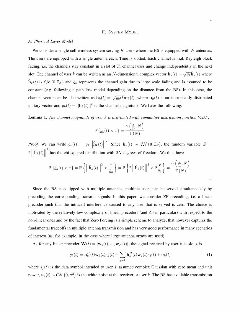
II. SYSTEM MODEL

A. Physical Layer Model

We consider a single cell wireless system serving K users where the BS is equipped with N antennas.

The users are equipped with a single antenna each. Time is slotted. Each channel is i.i.d. Rayleigh block

fading, i.e. the channels stay constant in a slot of Ts channel uses and change independently in the next

slot. The channel of user k can be written as an N -dimensional complex vector hk(t) =√gkhk(t) where

hk(t) ∼ CN (0, IN ) and gk represents the channel gain due to large scale fading and is assumed to be

constant (e.g. following a path loss model depending on the distance from the BS). In this case, the

channel vector can be also written as hk(t) =√gk(t)uk(t), where uk(t) is an isotropically distributed

unitary vector and gk(t) = ||hk(t)||2 is the channel magnitude. We have the following:

Lemma 1. The channel magnitude of user k is distributed with cumulative distribution function (CDF) :

P {gk(t) < x} =γ(xgk

;N)

Γ (N).

Proof. We can write gk(t) = gk

∣∣∣∣∣∣hk(t)∣∣∣∣∣∣2. Since hk(t) ∼ CN (0, IN ), the random variable Z =

2∣∣∣∣∣∣hk(t)∣∣∣∣∣∣2 has the chi-squared distribution with 2N degrees of freedom. We thus have

P {gk(t) < x} = P{∣∣∣∣∣∣hk(t)∣∣∣∣∣∣2 < x

gk

}= P

{2∣∣∣∣∣∣hk(t)∣∣∣∣∣∣2 < 2

x

gk

}=γ(xgk

;N)

Γ (N).

Since the BS is equipped with multiple antennas, multiple users can be served simultaneously by

precoding the corresponding transmit signals. In this paper, we consider ZF precoding, i.e. a linear

precoder such that the intracell interference caused to any user that is served is zero. The choice is

motivated by the relatively low complexity of linear precoders (and ZF in particular) with respect to the

non-linear ones and by the fact that Zero Forcing is a simple scheme to analyze, that however captures the

fundamental tradeoffs in multiple antenna transmission and has very good performance in many scenarios

of interest (as, for example, in the case where large antenna arrays are used).

As for any linear precoder W(t) = [w1(t), ...,wK(t)], the signal received by user k at slot t is

yk(t) = hHk (t)wk(t)sk(t) +∑j 6=k

hHk (t)wj(t)sj(t) + nk(t) (1)

where sj(t) is the data symbol intended to user j, assumed complex Gaussian with zero mean and unit

power, nk(t) ∼ CN(0, σ2

)is the white noise at the receiver or user k. The BS has available transmission

7

power P , that is tr(WWH) ≤ P . The achievable rate of user k at slot t is rk(t) (bits/channel use), which

depends on the corresponding signal-to-noise ratio (SNR) at time t. We will assume that the achievable

rates can take values from the set R = {R1, ..., Rl, .., RL}, with R1 = 0, Rl−1 < Rl and RL <∞; this

is the case in practice as a finite number of modulation and coding schemes are used for transmission.

In addition, we assume that the possible rate levels are known to the BS and mobiles, which is rather

reasonable since they are specified by the communications protocol used. Also we assume that rate

Rl can be supported if the signal-to-interference-plus-noise ratio (SINR) at the receiver is above some

appropriately defined threshold Sl.

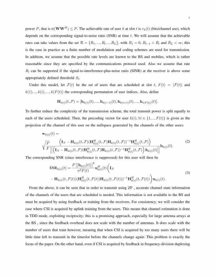
Under this model, let F(t) be the set of users that are scheduled at slot t, F (t) = |F(t)| and

k(1), .., k(i), ..., k(F (t)) the corresponding permutation of user indices. Also, define

Hk(i)(t,F) = [hk(1)(t), ...,hk(i−1)(t),hk(i+1)(t), ...,hi(F (t))(t)].

To further reduce the complexity of the transmission scheme, the total transmit power is split equally to

each of the users scheduled. Then, the precoding vector for user k(i),∀i ∈ {1, .., F (t)} is given as the

projection of the channel of this user on the nullspace generated by the channels of the other users:

wk(i)(t) =√P

F

(IN −Hk(i)(t,F)(HH

k(i)(t,F)Hk(i)(t,F))−1HHk(i)(t,F)

)∣∣∣∣∣∣(IN −Hk(i)(t,F)(HH

k(i)(t,F)Hk(i)(t,F))−1HHk(i)(t,F)

)hk(i)(t)

∣∣∣∣∣∣hk(i)(t).(2)

The corresponding SNR (since interference is suppressed) for this user will then be

SNRk(i)(t) =P∣∣∣∣hk(i)(t)

∣∣∣∣2σ2F (t)

uHk(i)(t)

(IN

−Hk(i)(t,F(t))(HHk(i)(t,F(t))Hk(i)(t,F(t)))−1HH

k(i)(t,F(t))

)uk(i)(t).

(3)

From the above, it can be seen that in order to transmit using ZF , accurate channel state information

of the channels of the users that are scheduled is needed. This information is not available to the BS and

must be acquired by using feedback or training from the receivers. For consistency, we will consider the

case where CSI is acquired by uplink training from the users. This means that channel estimation is done

in TDD mode, exploiting reciprocity; this is a promising approach, especially for large antenna arrays at

the BS , since the feedback overhead does not scale with the number of antennas. It does scale with the

number of users that train however, meaning that when CSI is acquired by too many users there will be

little time left to transmit in the timeslot before the channels change again: This problem is exactly the

focus of the paper. On the other hand, even if CSI is acquired by feedback in frequency-division duplexing

8

(FDD) mode, the BS must wait for the feedback from the users to be received before precoding [5]. Also

under our model of i.i.d. block fading channels, outdated feedback is not useful. The above imply that

the main ideas and results of the analysis presented can be useful even in systems with feedback in FDD

mode, assuming accurate channel estimation from the users’ side, enough bit rate in the reverse link for

perfect CSI in the BS after the feedback procedure and that the bandwidth in the uplink is not enough

for all users to feed back simultaneously in parallel channels. In addition, we will assume throughout this

paper that there are no errors in the channel estimation, in order to focus on the impact of time needed

for training in our system.

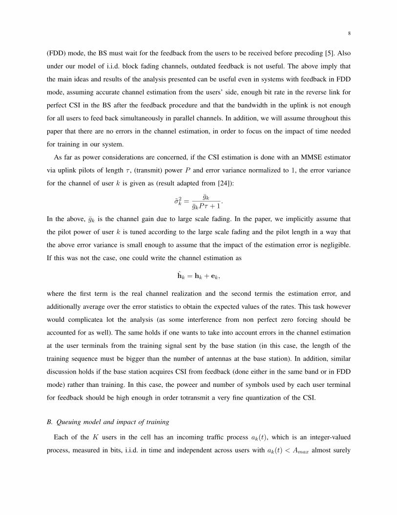
As far as power considerations are concerned, if the CSI estimation is done with an MMSE estimator

via uplink pilots of length τ , (transmit) power P and error variance normalized to 1, the error variance

for the channel of user k is given as (result adapted from [24]):

σ2k =

gkgkPτ + 1

.

In the above, gk is the channel gain due to large scale fading. In the paper, we implicitly assume that

the pilot power of user k is tuned according to the large scale fading and the pilot length in a way that

the above error variance is small enough to assume that the impact of the estimation error is negligible.

If this was not the case, one could write the channel estimation as

hk = hk + ek,

where the first term is the real channel realization and the second termis the estimation error, and

additionally average over the error statistics to obtain the expected values of the rates. This task however

would complicatea lot the analysis (as some interference from non perfect zero forcing should be

accounted for as well). The same holds if one wants to take into account errors in the channel estimation

at the user terminals from the training signal sent by the base station (in this case, the length of the

training sequence must be bigger than the number of antennas at the base station). In addition, similar

discussion holds if the base station acquires CSI from feedback (done either in the same band or in FDD

mode) rather than training. In this case, the poweer and number of symbols used by each user terminal

for feedback should be high enough in order totransmit a very fine quantization of the CSI.

B. Queuing model and impact of training

Each of the K users in the cell has an incoming traffic process ak(t), which is an integer-valued

process, measured in bits, i.i.d. in time and independent across users with ak(t) < Amax almost surely

9

for some finite constant Amax. This quantity is assumed to be known to the scheduler and users. The mean

rate of this process is E{ak(t)} = λk. Data for user k is stored in a respective buffer until transmission

and let qk(t) denote its size in bits at the beginning of slot t.

Denote now zk(t) as the schedule in timeslot t, that is zk(t) = 1 if user k is scheduled for this timeslot

(i.e. if user k has actually reported its channel to the BS ). We are under the constraints that (i) F (t)

users are scheduled at each timeslot, with F (t) ≤ N (ii) for every channel the BS schedules a user

whose channel state is known at the maximum possible rate it can support (that is ensuring transmission

without errors). In addition, we will denote here τ(t) the number of channel uses used for training and

signalling in the slot t. This means that data is transmitted for a scheduled user for (Ts − τ(t)) channel

uses, therefore, if the rate supported to user k at timeslot t is rk(W(t),H(t)) ∈ R bits per channel use,

the corresponding service process will be (Ts − τ(t))rk(W(t),H(t)) bits 2. The queues then evolve as

follows, ∀k ∈ {1, ..,K}:

qk(t+ 1) = [qk(t)− b(Ts − τ(t))rk(W(t),H(t))czk(t)]+ + ak(t), t ≥ 0

qk(0) = ak(−1).

(4)

In the above, ak(−1) is defined as a random variable drawn from the distribution of ak(t), t ≥ 0. This

constraint actually means that we start measuring time after the first arrivals in the queues so that the

queues do not start empty (and the broadcast of the queue lengths at time t = 0 not to be the zero

queue). This is done for more convenience in analysing the proposed algorithm, however, since we are

interested in the case when the system is left running for long enough for the corresponding Markov

chains to reach their invariant distribution (i.e. t→∞) and the arrival processes are bounded, the choice

of the initial condition does not really affect our results.

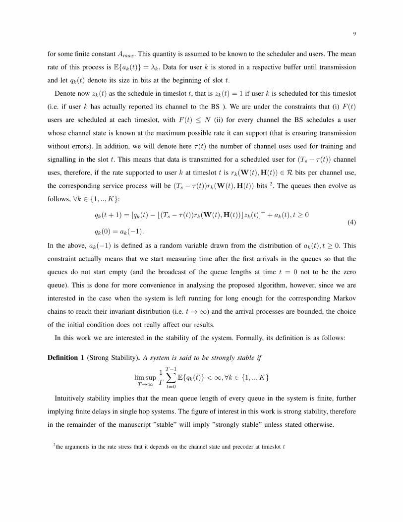
In this work we are interested in the stability of the system. Formally, its definition is as follows:

Definition 1 (Strong Stability). A system is said to be strongly stable if

lim supT→∞

1

T

T−1∑t=0

E{qk(t)} <∞, ∀k ∈ {1, ..,K}

Intuitively stability implies that the mean queue length of every queue in the system is finite, further

implying finite delays in single hop systems. The figure of interest in this work is strong stability, therefore

in the remainder of the manuscript ”stable” will imply ”strongly stable” unless stated otherwise.

2the arguments in the rate stress that it depends on the channel state and precoder at timeslot t

10

The above definition holds for a fixed mean arrival rates and resource allocation policy, and leads to

the concept of a stability region.

Definition 2 (Stability Region). The stability region Λ of a resource allocation policy is defined as the

set of vectors of mean arrival rates for which the system is stable under this policy. Furthermore, an

algorithm that achieves the maximum possible stability region is called throughput optimal.

For the rest of the paper, when describing stability regions we will mean that the system is stable in

the interior of the calculated region. The behaviour on the boundary is not examined - usually for the

boundary points the system is stable in at least a weaker sense, i.e. mean rate stable [25]. If the arrivals

and service rate processes are such that the Markov chain is irreducible and aperiodic with a single

communicating class and the control actions are taken as functions of the queue state only, a necessary

condition for strong stability is that the Markov chain is positive recurrent and the mean service rates

(under the invariant distribution) are bigger than the mean arrival rates. Since we are considering the

interiors of the stability regions, i.e. not examining the cases where the mean arrival rates qre equalto

the mean service rates, the above condition is sufficient for our analysis. In a stable system the users

experience finite delays, therefore stability is a relevant aspect for data services and users with large

delay tolerance. Uplink training affects essentially the service rate, and thus the stability region, in two

ways: First, more time devoted to training leads to lower service rate for the users actually scheduled in

the timeslot. On the other hand, if more users participate in the training, more users can get scheduled

in a timeslot, thus overall a user can get higher mean service rate. The focus of this paper is, then, this

tradeoff and how to efficiently design user selection strategies to achieve large stability regions.

For simplicity, we only consider schemes where all users whose CSI is acquired get scheduled. Also,

as mentioned before, transmit power is allocated equally to scheduled users. The first assumption is

common in the literature concerning MIMO broadcast systems, where all ”active users” are scheduled,

see e.g. [5]. In addition, even in the case of full CSI without any cost, the highest stability region would

be given from solving a weighted sum maximization problem in each timeslot (in accordance to the

MaxWeight rule [26], [27]). Joint scheduling and power control even in this ideal case is a hard problem,

especially in our model with finite rate set (some algorithms like iterative waterfilling [11] have been

proposed but using the information theoretic capacity for the service rates). Adding the cost of feedback

on top of it would make the problem more complicated and result in a solution of high computational

complexity (see e.g. [28] for the problem in the single antenna case, where only approximations of the

optimal solution are implementable in practice). The problem then reduces to finding strategies to choose

11

the ”active” users at each time slot.

III. PROPOSED POLICIES FOR USER SELECTION

In this section we present in detail the scheduling and training policies to be analyzed in the present

work. Before proceeding in the descriptions, we define R0 (bits per channel use) the rate at which the

control information from the BS to the users can be broadcasted. Further, we assume that when F

users perform the uplink training, they use orthogonal pilot of length βF channel uses. β is an integer

system parameter, not smaller than 1 (for the pilots to be indeed orthogonal). Greater length of training

sequences implies that the training symbols should have less power (for the same quality of estimation)

so this parameter can be tuned according to the power capabilities of the user terminals. Finally, downlink

pilots are assumed of a length of βp channel uses. Since at least a downlink pilot and the uplink pilots

must be used, the maximum number of users to be scheduled is the maximum number of users that can

participate in training within the duration of the timeslot, that is

Fmax = min

{N,

⌊Ts − βpβ

⌋}. (5)

In practice this number may be actually lower, for example it is usually desirable that at least half of the

timeslot is used for data transmission [29].

In the following subsections, we present in detail the scheduling and feedback schemes examined. For

the reader’s convenience, we have put the list of variables included in the paper in Table I.

A. Centralized policy

Since the channel statistics are known, one approach is to let the BS decide which users to acquire

CSI from and schedule based on the expectation of the rate they receive. Each expectation is found over

the joint probability distribution of the channel realizations of all users and its expression is given in

Section IV-A. For this scheme, the BS sends a downlink pilot to allow the users to estimate their channel

and decode the control messages. After the pilot, there is a control phase, where the BS broadcasts the

identification numbers (IDs) of the users that will get scheduled at this timeslot. For each user selected

βc =log2K

R0

channel uses are needed. In addition, there must be a way for the users to know that the control part is

over and that those among them that are scheduled should start training. Here we propose that the signal

for that is the BS staying silent for one channel use. An alternative, and perhaps more robust, way would

12

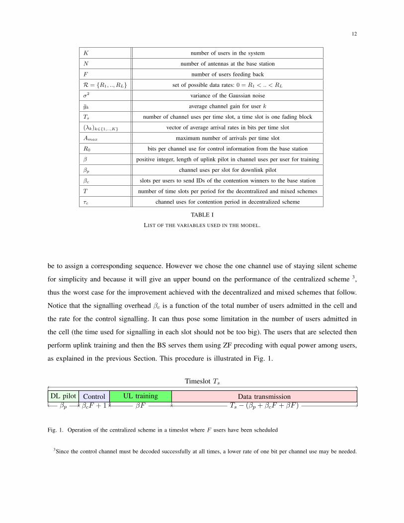
K number of users in the system

N number of antennas at the base station

F number of users feeding back

R = {R1, .., RL} set of possible data rates: 0 = R1 < .. < RL

σ2 variance of the Gaussian noise

gk average channel gain for user k

Ts number of channel uses per time slot, a time slot is one fading block

(λk)k∈{1,..,K} vector of average arrival rates in bits per time slot

Amax maximum number of arrivals per time slot

R0 bits per channel use for control information from the base station

β positive integer, length of uplink pilot in channel uses per user for training

βp channel uses per slot for downlink pilot

βc slots per users to send IDs of the contention winners to the base station

T number of time slots per period for the decentralized and mixed schemes

τc channel uses for contention period in decentralized scheme

TABLE I

LIST OF THE VARIABLES USED IN THE MODEL.

be to assign a corresponding sequence. However we chose the one channel use of staying silent scheme

for simplicity and because it will give an upper bound on the performance of the centralized scheme 3,

thus the worst case for the improvement achieved with the decentralized and mixed schemes that follow.

Notice that the signalling overhead βc is a function of the total number of users admitted in the cell and

the rate for the control signalling. It can thus pose some limitation in the number of users admitted in

the cell (the time used for signalling in each slot should not be too big). The users that are selected then

perform uplink training and then the BS serves them using ZF precoding with equal power among users,

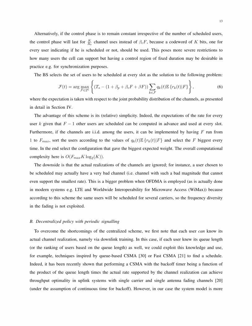
as explained in the previous Section. This procedure is illustrated in Fig. 1.

Timeslot Ts

DL pilotβp

ControlβcF + 1

UL trainingβF

Data transmissionTs − (βp + βcF + βF )

Fig. 1. Operation of the centralized scheme in a timeslot where F users have been scheduled

3Since the control channel must be decoded successfully at all times, a lower rate of one bit per channel use may be needed.

13

Alternatively, if the control phase is to remain constant irrespective of the number of scheduled users,

the control phase will last for KR0

channel uses instead of βcF , because a codeword of K bits, one for

every user indicating if he is scheduled or not, should be used. This poses more severe restrictions to

how many users the cell can support but having a control region of fixed duration may be desirable in

practice e.g. for synchronization purposes.

The BS selects the set of users to be scheduled at every slot as the solution to the following problem:

F(t) = arg maxF∈2K

{(Ts − (1 + βp + βcF + βF ))

∑k∈F

qk(t)E {rk(t)|F}

}, (6)

where the expectation is taken with respect to the joint probability distribution of the channels, as presented

in detail in Section IV.

The advantage of this scheme is its (relative) simplicity. Indeed, the expectations of the rate for every

user k given that F − 1 other users are scheduled can be computed in advance and used at every slot.

Furthermore, if the channels are i.i.d. among the users, it can be implemented by having F run from

1 to Fmax, sort the users according to the values of qk(t)E {rk(t)|F} and select the F biggest every

time. In the end select the configuration that gave the biggest expected weight. The overall computational

complexity here is O(FmaxK log2(K)).

The downside is that the actual realizations of the channels are ignored; for instance, a user chosen to

be scheduled may actually have a very bad channel (i.e. channel with such a bad magnitude that cannot

even support the smallest rate). This is a bigger problem when OFDMA is employed (as is actually done

in modern systems e.g. LTE and Worldwide Interoperability for Microwave Access (WiMax)) because

according to this scheme the same users will be scheduled for several carriers, so the frequency diversity

in the fading is not exploited.

B. Decentralized policy with periodic signalling

To overcome the shortcomings of the centralized scheme, we first note that each user can know its

actual channel realization, namely via downlink training. In this case, if each user knew its queue length

(or the ranking of users based on the queue length) as well, we could exploit this knowledge and use,

for example, techniques inspired by queue-based CSMA [30] or Fast CSMA [21] to find a schedule.

Indeed, it has been recently shown that performing a CSMA with the backoff timer being a function of

the product of the queue length times the actual rate supported by the channel realization can achieve

throughput optimality in uplink systems with single carrier and single antenna fading channels [20]

(under the assumption of continuous time for backoff). However, in our case the system model is more

14

complicated because the users do not know their queue lengths and because of multiple antennas in the

BS, more than one user can be scheduled simultaneously. Our proposed schemes, detailed in the next

paragraph, are based on two ideas: (i) the BS periodically broadcasts the (suitably quantized) values of

the queue lengths and (ii) the BS decides on the number of users to be scheduled and based on that lets

the users contend using the queue length information they have and an estimate of their achievable rate

based on channel state realization.

1) Algorithm description: To begin with, every T timeslots, that is at time 0, T, 2T, ...,mT, ... the BS

broadcasts quantized versions of the queue lengths of the users at the beginning of this slot, i.e. broadcasts

a quantization of the vector q(mT ),m = 0, 1, ..., the restriction being that T is a finite number. The

quantization of the queue lengths is discussed in detail in Section III-B2. In addition, the BS broadcasts

the number F (mT ) of users to report the channel each timeslot for the next T −1 consecutive timeslots.

No data transmission at this timeslot takes place in order to make broadcasting this information possible

(with the BS adopting e.g. uniform precoding for transmission).

Denote now by q(t) := q(T b tT c) to be the most recent information about their queue state that the

users have. At each timeslot the BS sends a downlink pilot with duration βp channel uses so that the

users can estimate their channels and lets a period of τc channel uses for the users to contend for channel

access. Assuming that contention can be done in continuous time and with signals of negligible duration

(this assumption has been implicitly used in recent works dealing with Fast CSMA over fading channels

[21], [19]), user k waits until time

τ ′k =τ ′c

qk(t)E{rk(t)|gk(t), F (t)}. (7)

In the above equations, the times are expressed in time units (i.e. ms or µs). The denominator is the

latest broadcasted value of the queue length of this user times the expectation of the rate the user will

get if it is scheduled, given its own channel realization (we have defined here gk(t) = ||hk(t)||2). This

computation is detailed in the Section IV-A, and for an environment with Rayleigh fading (the case we

examine here) can be done in a totally decentralized manner. Note that under this scheme, the F users

with the biggest values of qk(t)E{rk(t)|gk(t), F (t)} are the ones that get actually scheduled.

Once the contention period is over, the F first users to have a signal broadcasted feed back their IDs in

a TDMA manner, e.g. in the sequence in which they sent the contention signals (under the assumptions

on continuous time contention and very short signals the users can know their place in the sequence).

These users then perform uplink training and the BS transmits to them using Zero Forcing. The total time

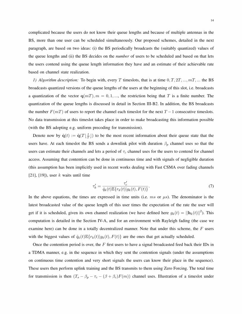
for transmission is then (Ts − βp − τc − (β + βc)F (m)) channel uses. Illustration of a timeslot under

15

this policy is given in Fig. 2.

Timeslot Ts

DL pilotβp

Cont.τc

IDs ULβcF

UL trainingβF

Data transmissionTs − (βp + τc + βcF + βF )

Fig. 2. Operation of the decentralized scheme in a data timeslot where the Base Station has signalled that F users are to be

scheduled

What remains to be specified is the number of users to feed back in every period {mT+1, ..., (m−1)T}.

As stated before, this decision is taken in the beginning of timeslot mT , based on the corresponding queue

length information and channel statistics. Here we consider that the number of users to get scheduled is

given as the solution of the following problem.

F ∗(m) = arg maxF=1,..,Fmax

{(Ts − βp − τc − (β + βc)F )Eg(t)

{maxF :|F|=F

∑k∈F

qk(mT )E {rk(mT )|gk(t), F}

}}.

(8)

In the above, the outer expectation is with respect to the joint distribution of the channel magnitudes while

the inner expectation is with respect to the joint distributions of the channel directions (for the channels

of all users in the system). A way to do these calculations is to use the recently proposed framework in

[31], [32] for partial sums of order statistics of non-identically distributed random variables.

2) Queue length quantization scheme: As noted in the description of the algorithm, the BS broadcasts

quantized versions of the queue lengths of the users. This quantization is essential because, as noted in

the beginning of the Section the rate at which the BS can broadcast signalling information is R0 bits per

channel use; this means that if a slot is used for signalling, at most TsR0 bits can be sent to the users.

Given that the BS should broadcast K queue lengths and how many users are to feed back, the number

of bits bq used for quantization of each queue should satisfy the following:

Kbq + log2 Fmax ≤ TsR0. (9)

The above inequality poses limitations as to how many users can be supported by the system if it operates

under this scheduling policy and a limitation to the accuracy of the queue length feedback for a given

number of users in the cell. However, if multiple antennas and carriers are used, this limitation is not

very severe.

16

We now detail the way the queue lengths are actually quantized for a given number of bits per user,

bq. To this end, we define

Q = max {TRL, TAmax} (10)

and the intervals [0, Q], [Q, 2Q], ..., [(p−1)Q, pQ], .... Note that Q is the biggest change that can possibly

happen to a queue length after T slots (the queue will decrease by at most TRL-if at every slot is served

at the maximum rate with no further arrivals- and increase by at most by TAmax-if it s not served at all

and has the maximum possible arrivals at each slot). Therefore, every T slots each queue length will be

in one of the aforementioned intervals, and furthermore, given that at mT a queue length was at the p-th

interval, at (m + 1)T it will be at intervals p − 1, p or p + 1. The idea is then to set the quantization

interval to [0, Q] at the beginning and inform each user every T slots if it stays in the same interval

of one of the neighbouring intervals (this can be done at a signalling as low as 2 bits per user or even

1.5K bits in total). Then, the quantized queue length is sent, assuming uniform quantization within each

interval using the rest of the signalling bits available. More concretely, if bq bits per user are used for

quantization 2 bits are used to denote the quantization interval and the rest are used to point to one of the

2bq−2 levels within the interval. If bq = 2, then the middle value of the interval is used as an estimation

of the queue length. Note that this way, the difference between each of the broadcasted queue lengths,

denoted by q(mT ) and the corresponding real queue length from q(mT ) is at most Q .

Finally, some remarks are in order. First, we have assumed that the control information broadcasted by

the BS are always decodable at the user terminals. This is a rather frequent and reasonable assumption in

the literature (i.e. that signalling and control data are transmitted without errors). In practice, control data

are transmitted using low rate modulations and strong coding schemes. We can also always assume that

we do downlink power control for the signalling information. In addition, if the number of carriers and

antennas is high, the diversity of the system is so big that control data can always be received successfully

even if some channels of the users are in deep fade (also, users with very bad average channel conditions

should not be admitted into the cell). Accurate estimation of the users channel can be similarly argued

by using high power pilots.

C. Mixed Policy: Combining Centralized and Decentralized Schemes

The decentralized approach to the user selection problem should lead to users with better channel

conditions being selected in general, however it requires some extra time overhead for the contention

period. In some cases, some queues may be empty or a few queues may be much bigger than others. If

17

this happens it may be better for the users with the much bigger queues to be scheduled for the T − 1

timeslots without any additional signalling overhead. Note that since the same users get scheduled every

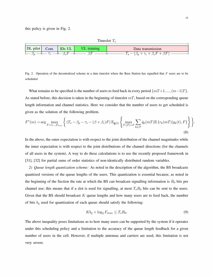
T − 1 consecutive slots, no overhead for their IDs must be used either. The operation of this scheme in

a data timeslot is illustrated in Fig. 3 4. We will refer to this scheme as ”periodic centralized policy” for

the rest of the paper.

Timeslot Ts

DL pilotβp

UL trainingβF

Data transmissionTs − (βp + βF )

Fig. 3. Operation of centralized scheme with periodic user selection in a data timeslot where the Base Station has signalled a

set of F users to be scheduled

The set of users to schedule according to this periodic centralized policy is set as

F∗(m) = arg maxF∈2K

{(Ts − (βp + βF ))

∑k∈F

qk(mT )E {rk(t)|F}

}. (11)

The mixed policy here is, therefore, that the BS at every slot t = mT,m = 0, 1, ... decides that, for

the next T −1 slots, either the decentralized policy will be used, with the optimal number of users to get

scheduled as given by eq. (8) or select a set F(m) of users to schedule according to the maximization

in eq. (11). This decision is made based on which of the two policies will maximize the quantity

E{∑K

k=1 qk(mT )(Ts − τ(t))rk(t)

∣∣∣∣q(mT )

}, with the expectation taken over the channel distributions

(which affect the outcomes of the policies). More concretely, let F ∗(m) be given by (8) and F∗(m) be

given by (11). Then, the BS selects the decentralized scheme with F ∗(m) users to get scheduled if

(Ts − βp − τc − (β + βc))Eg(t)

{max

F :|F|=F ∗(m)

∑k∈F

qk(mT )E {rk(mT )|gk(t), F}

}

≤ (Ts − (βp + βF ))∑

k∈F∗(m)

qk(mT )E {rk(t)||F∗(m)|}

and the centralized scheme with the users in F ∗(m) otherwise.

This policy should have a bigger stability region than either of the two policies mentioned before in

this Section, since it essentially combines the ideas behind both. However, we would like to point out

that the decentralized policy alone can achieve points that can not be achieved by the centralized (or the

4The DL pilot is still needed for the users to set the power of their training sequences such that the SNR in the reverse link

suffices for perfect estimation

18

version of the centralized policy used in the mixed scheme) policy. Normally while applying the mixed

policy, the decentralized scheme should be the one most frequently selected, with the centralized mode

selected in special cases (for example, when few queues are not empty or there is a queue that is much

bigger than all the others). It needs 1 additional bit of signalling compared to the other policies, in order

to inform the users if the centralized or decentralized scheme will be employed. In addition, the BS needs

to broadcast the number F of users to be scheduled in the decentralized policy if used (log2(Fmax) bits)

or the users to get scheduled in case the centralized policy is used (min {K,Fmax log2K} bits). Since

Fmax ≤ K, there must hold

Kbq + min {K,Fmax log2K} ≤ TsR0, (12)

which gives a bound on the number of users to be admitted to the cell in order to operate under the

mixed policy.

IV. CALCULATION OF PARAMETERS AND STABILITY RESULTS

In this Section we give the expressions for the SNR (and subsequently rate) distributions. Also, we

give some useful lemmas about stability of systems where control decisions are done periodically and

not in a slot-per-slot basis.

A. Calculation of average rates

The decentralized scheme requires that every user should calculate their average rate given their current

channel state realization, as seen by eq. (7). Indeed, since the system operates under isotropic fading

directions, we can calculate the probability distribution over the other users’ channels and zero forcing

precoding of a user’s SNR given its channel. We have:

Proposition 2. The probability that the received SNR at user k exceeds s given its channel strength and

that this user and other F − 1 users are scheduled is given by

P {SNRk(t) > S|gk(t), F} = P {SNRk(t) > S|hk(t), F}

= 1− IB(

Fσ2

Pgk(t)S;N − F + 1, F − 1

).

(13)

This distribution is with respect to the direction of the channel of user k and the channels of the other

users that get scheduled.

Proof. Please refer to Appendix A for the proof.

19

From the above result and the proof we can see that only the magnitude and not the direction of the

channel realization comes into the equation. In addition, the long-term statistics of the other users do not

play any part in the computation either. Intuitively these remarks are due to the isotropic direction of the

channel vectors. Indeed, since we are considering ZF precoding, the loss of SNR comes due to the fact

that the channels are not orthogonal, therefore the demand of causing zero interference can constrain a

lot the precoder selection. Since the directions are isotropic, knowledge of one channel direction does not

imply anything about how nullspace of the other users should behave. A consequence of these remarks

is that a user can actually calculate this distribution (and hence the average rate he will get given its

channel) with only the knowledge that the whole system operates under Rayleigh fading.

In the centralized scheme, where the BS does not have knowledge of the magnitude realization of the

channels, the probability that the SNR of user k exceeds S when F − 1 other users are scheduled is the

following [15], [33]5

Proposition 3. Given a number of users to be scheduled, F , the probability that the SNR of user k

exceeds S is given as

P {SNRk(t) > S|F} = 1−γ(Fσ2

gkPS;N − F + 1

)Γ(N − F + 1)

.

From the results of Propositions 2 and 3 we can find the average rates conditioned on the channel real-

ization of user k and the expected rate of this user without knowing the channel realization, respectively.

More concretely, if we define

L0,k(t, F ) = max

{l ∈ 1, ..., L : Sl ≤

gk(t)P

Fσ2

}, (14)

i.e. the index of the highest rate that could be supported by user k if he is scheduled and his channel is

orthogonal to the channels of the other F − 1 scheduled users, we have:

E {rk(t)|F, gk(t)} =

L0,k(t,F )∑l=1

RlP {Sl ≤ SNRk(t) < Sl+1|F, gk(t)}

=

L0,k(t,F )∑l=1

Rl (P {SNRk(t) ≥ Sl|F, gk(t)} − P {SNRk(t) ≥ Sl+1|F, gk(t)}) .

(15)

5It can also be calculated by integrating (13) for gk(t) from zero to infinity. Although we could not obtain the exact form

given in Proposition 3, numerical results indicate that the numerical values are the same with either method. We will use the

latter expression since it is in a closed form

20

and

E {rk(t)|F} =

L∑l=1

Rl (P {SNRk(t) ≥ Sl|F} − P {SNRk(t) ≥ Sl+1|F}) . (16)

Notice that, since the statistics are assumed known, the rates in (16) can be calculated only once and

used by the BS for the centralized scheme.

B. Stability results

In this subsection we are interested in deriving some stability results for the system under the policies

where slots {0, T, T + 1, ..,mT, ..} are used for signalling and/or broacasting of the queue lengths. First,

we define the queueing system that results when examining the original system at time instances 0, T, ...,

i.e. at the beginning of the slot in which the broadcasting takes place. Formally:

q(m) := q(mT ),m = 0, 1, 2, .... (17)

The equations regarding the evolution of this system are, thus ∀k ∈ {1, ...,K}:

qk(m+ 1) = qk(m) +

T−1∑t=0

ak(mT + t)−T−1∑t=1

zk(mT + t)µk(mT + t) +

T−1∑t=1

yk(mT + t) (18)

where zk(t) is the indicator function, set to 1 if user k is scheduled in timeslot t and zero otherwise, µk(t)

is the total number of bits assigned for transmission to user k at timeslot t (that is µk(t) = rk(t)(Ts−τ(t))

(recall that τ(t) is the total time of the slot used for pilot transmission, coordination and training), and

yk(mT + t) = [zk(mT + t)µk(mT + t)− qk(mT + t)]+ the number of ”wasted” bits if the offered rate

at one timeslot is bigger than the available bits in the buffer. Note that the process q(m) is a discrete

time Markov chain evolving on a countable state space. The following result holds:

Lemma 4. The system q(t) is strongly stable if and only if the system q(m) is strongly stable.

Proof. Assume first that q(t) is strongly stable. We have 1M

∑M−1m=0 E{qk(m)} ≤ T 1

MT

∑T (M−1)τ=0 E{qk(τ)}

therefore

limM→∞

sup1

M

M−1∑m=0

E{qk(m)} ≤ T limM→∞

sup1

MT

T (M−1)∑τ=0

E{qk(τ)} < +∞,

where the second inequality follows from the assumption. Therefore q(m) is indeed strongly stable.

Assume now that q(m) is strongly stable. We can write

limt→+∞

sup1

t

t−1∑τ=0

E{qk(τ)} = limM→+∞

sup1

MT

MT−1∑τ=0

E{qk(τ)}

= limM→∞

sup

(1

MT

M−1∑m=0

E{qk(mT )}+1

MT

M−1∑m=0

T−1∑τ ′=1

E{qk(mT + τ ′)}

).

(19)

21

Since q(m) is strongly stable and q(m) = q(mT ), there exists some 0 < C0 < ∞ such that ∀k ∈

{1, ..,K} :

limM→∞

sup1

MT

M−1∑m=0

E{qk(mT )} ≤ C0

T. (20)

Also, note that ∀τ ′ ∈ {1, .., T − 1}, ∀m = 0, 1, .... it holds qk(mT + τ ′) ≤ qk(mT ) + τ ′Amax. This

implies that, ∀m = 0, 1, 2, ... we have∑T−1

τ ′=1 E{qk(mT + τ ′)} ≤ E{qk(mT )}+ (T−1)T2 Amax. Replacing

we get

limt→+∞

sup1

t

t−1∑τ=0

E{qk(τ)} ≤ limM→∞

sup

(2

MT

M−1∑m=0

E{qk(mT )}+T (T − 1)

2Amax

)

≤ 2C0

T+T (T − 1)

2Amax <∞,

which implies that q(t) is stable.

The above Lemma implies that a throughput optimal policy for the process q(m) should be also

throughput optimal for the original system.

Define now V (x) = 12

∑Kk=1 x

2k a Lyapunov function and ∆V (x) its drift, i.e.

∆V (x) = E {V (q(m+ 1))− V (q(m))|q(m) = x} . (21)

The expectation is over the arrival and channel processes as well as the possibly randomized feedback

policy (i.e. the set of F users that feed back). Then the following holds for the drift of the sampled

system:

Lemma 5. The drift of the quadratic Lyapunov function for the system q(m) under a scheduling policy

π is upper bounded as follows (note that the number of users to feed back, F is included in the policy):

∆Vπ(q(m)) ≤ B + T

K∑k=1

qk(m)λk − (T − 1)

K∑k=1

qk(m)E {µπk(m)|q(m)} (22)

where µπk(m) is the rate of user k in any of the slots mT + 1, ...,mT + (T −1) for a given channel state

realization and outcome of the policy π (i.e. set of users actually fed back), B is a constant depending

only on the system parameters. The expectation is taken over the joint distribution of the channels and

possible randomization of the policy.

Proof. Please refer to Section B in the Appendix of this paper for the proof.

As a final remark, we note that the same stability results with Lemma 4 hold for the system operating

under the centralized policy as well. That is, the system operating under the centralized policy is stable

22

if and only if the system that results from sampling the queue lengths of the original at timeslots mT is

strongly stable;the proof is essentially the same as the proof of Lemma 4.

V. A SPECIAL CASE: THE 2-USER MISO BC WITH SINGLE RATE

In this Section we will consider a simple case, namely a system with K = 2 users with identical

channel statistics (i.i.d. Rayleigh with mean power gain g) where a user gets rate R bits per channel use

if SNR exceeds the threshold S and zero otherwise. This setting is of interest as the stability regions

admit easy mathematical expressions and can be plotted, thus giving some insight on the outcomes of

the policies.

To begin with, we define some parameters to be used frequently in the sequel. Define the probabilities

that a user’s SNR exceeds the threshold if only one or both users are scheduled as p(1) and p(2),

respectively. Since the channels are statistically identical for both users, these probabilities are the same

for any of them. The numerical values of these probabilities are given by

p(1) = 1−γ(σ2SP g ;N

)Γ (N)

p(2) = 1−γ(

2σ2

gP S;N − 1)

Γ(N − 1).

(23)

These expressions are derived by specializing the results in Sections II and IV for F = 2 and gk = g.

The system parameters are the same as in the original description: Downlink training requires βp channel

uses and uplink training requires pilots of length β channel uses for each user.

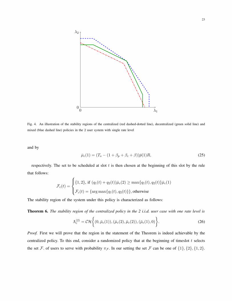
We now turn to characterizing the form and stability region of each policy. The general shapes of the

policies are sketched in Fig. 4 that follows, and Fig. 5 in the next Section depicts a numerical example

with specific values of the parameters.

A. Centralized policy

In this policy, in every slot t the transmitter selects either one or both the receivers to be scheduled. In

the latter case, there is an overhead of 2βc channel uses to broadcast the IDs of the two users and in the

former, of βc + 1 to broadcast the ID of the scheduled user and a signal that the control period is over.

The expected rate that a user gets if both users are scheduled or if this user only is scheduled at

timeslot t is given by

µc(2) = (Ts − (βp + 2βc + 2β))p(2)R (24)

23

λ10

λ2

0

Fig. 4. An illustration of the stability regions of the centralized (red dashed-dotted line), decentralized (green solid line) and

mixed (blue dashed line) policies in the 2 user system with single rate level

and by

µc(1) = (Ts − (1 + βp + βc + β))p(1)R, (25)

respectively. The set to be scheduled at slot t is then chosen at the beginning of this slot by the rule

that follows:

Fc(t) =

{1, 2}, if (q1(t) + q2(t))µc(2) ≥ max{q1(t), q2(t)}µc(1)

Fc(t) = {arg max{q1(t), q2(t)}}, otherwise

The stability region of the system under this policy is characterized as follows:

Theorem 6. The stability region of the centralized policy in the 2 i.i.d. user case with one rate level is

Λ(2)c = CH

{(0, µc(1)), (µc(2), µc(2)), (µc(1), 0)

}. (26)

Proof. First we will prove that the region in the statement of the Theorem is indeed achievable by the

centralized policy. To this end, consider a randomized policy that at the beginning of timeslot t selects

the set F . of users to serve with probability πF . In our setting the set F can be one of {1}, {2}, {1, 2}.

24

The achievable stability region by this policy is

λ1 < π{1}µc(1) + π{1,2}µc(2) := µ1

λ1 < π{2}µc(1) + π{1,2}µc(2) := µ2

, (27)

with π{1} + π{2} + π{1,2} ≤ 1 and 0 ≤ πF ≤ 1. This is exactly the algebraic characterization of the set

(26).

Define now the quadratic Lyapunov function V (x) = x21 + x2

2. Its drift

∆V (q) = E {V (q(t+ 1))− V (q(t))|q(t) = q}

can be shown to be bounded as (with some positive constant B)

∆V (q) ≤ B −2∑

k=1

(qk(t)E{µk(t)} − qk(t)λk) ≤ B −2∑

k=1

qk(t)(µk − λk).

The second inequality follows by the definition of our centralized policy. From (27) it follows that

∀λ ∈ Λ(2)c ,∃ε > 0 such that ∆V (q) ≤ B − ε

∑2k=1 qk(t), hence the system under the centralized policy

is indeed stable for all mean arrival rates in the asserted region.

We then need to prove the converse, that is, if a centralized policy achieves stability, then the mean

arrival rate lies in (the interior of) the region given by (26). Indeed, assume that the system is stable for a

mean arrival rate vector λ. The centralized policy depends only on the queue lengths at the beginning of

slot t, which we denote by F(q). The assumptions, thus, on the channel and arrival processes make the

system a discrete time Markov chain with a single communicating class. In this case, stability implies

the existence of an invariant distribution π(q). The mean service rate user k gets is then equal to

limt→∞

1

t

t−1∑τ=0

µk(τ) = µc(1)∑

q∈Z2+:F(q)={k}

π(q) + µc(2)∑

q∈Z2+:F(q)={1,2}

π(q).

Since the sums are probabilities themselves, we can see that the service rate have the same form as in

(27). Also, since the system is assumed stable, there should be λk < limt→∞1t

∑t−1τ=0 µk(τ). From these

we conclude that λ ∈ Λ(2)c , completing the proof.

The stability region for the centralized scheduling algorithm looks like a trapeze with corner points

(0, 0), (0, µc(1)), (µc(2), µc(2)), (µc(1), 0) if it holds that µc(1) < 2µc(2) and like a triangle with corners

at (0, 0), (0, µc(1)), (µc(1), 0) otherwise. This follows from the fact that in the latter case only one user

will get scheduled.

25

B. Decentralized Policy

Let the time for contention be τc channel uses. For consistency, the contention period will be present

even if F = 2, i.e. when both users are to be scheduled (this will be improved by the mixed policy). From

the results of Section IV-B it suffices to look at the stability of the system examined in the beginning of

each signalling slot mT,m = 0, 1, ....

As described in Section III-B, the BS broadcasts the quantized queue lengths q1(mT ), q2(mT ) at time

mT . In the particular case with 2 users, the decision taken by the BS is to either select both users

(F (m) = 2) or signal that one user will be selected (F (m) = 1) and the user who will be scheduled is

the one with the lowest timer from eq. (7).

1) Contention procedure: If F (m) = 1, in each of these slots the receivers are given a contention

period of τc channel uses to decide which one is to be scheduled based on the (quantized and outdated)

queue length information they have and the realization of their channels. This can be done using a

contention scheme, assuming contention in continuous time e.g. like [21], where each user waits until timeτc

qk(m)rk(t) : if both have the same timer, e.g. the user with the smallest ID is scheduled. Another alternative,

that can be used thanks to our model, is to divide the contention period into minislots (TDMA manner)

where each receiver sends a signal in its corresponding minislot if its SNR is above the threshold S. If both

receivers send a signal, in their corresponding minislots, then the receiver with the largest broadcasted

queue length gets scheduled for training (this analysis/comparison can be done independently by each

receiver since the queue lengths of all receivers are broadcasted). Otherwise, if only one user sends a

signal in a minislot, then this user will be scheduled for training. Then, the user to be scheduled sends

its ID to the BS , taking βc channel uses, and trains. Using the above ”decentralized” procedure, the user

that will eventually get served in the slot will be the one with the maximum product of quantized queue

length at mT times achievable rate. Due to our model here, denoting SNR(1)k (t) = Pgk(t)

σ2 , the user to

be scheduled will be

• If ∀k = 1, 2 holds SNR(1)k (t) > S, then k∗(t) = arg max[q1(mT ), q2(mT )]

• The user for which SNR(1)k (t) > S otherwise

The scheduled receiver will always be given rate of R bits per channel use, except in the case where no

one has sufficiently high SNR, in which no receiver can be scheduled anyway. Defining the permutation

k(1), k(2), where qk(1)(mT ) ≥ qk(2)(mT ), the average service rates of these users under F = 1 for the

26

next T − 1 slots are

µd,(1)k(1) (t) = (Ts − (βp + τc + β))p(1)R := µd(1)

µd,(1)k(2) (t) = (Ts − (βp + τc + β))p(1)(1− p(1))R.

(28)

2) F(m)=2:Both users train just after the coordination period. The average rate per slot for each user

in this case will be

µd(2) = (Ts − (βp + τc + 2β))p(2)R (29)

Based on the above, the transmitter decides at t = mT the number of users to get scheduled for the

next T − 1 slots by:

F (m) =

2, if qk(1)(m) + qk(2)(m))µ

d,(1)k(1) (t) ≥

(qk(1)(m) + qk(2)(t)(1− p(1)))µd,(1)k(1) (t)

1, otherwise

In the case of F (m) = 1, the contention procedure is followed.

The stability region of this policy is described as follows :

Theorem 7. The stability region of the decentralized scheme for the 2 user MISO broadcast system with

a single rate level is

Λ(2)d =

(1− 1

T

)CH{

(0, µd(1)), (µd(1)(1− p(1)), µd(1)),

(µd(2), µd(2)), (µd(1), µd(1)(1− p(1))), (µd(1), 0)

}Proof. The proof consists in four parts. For the first two parts we compute the stability region for policies

that select all the time F = 2 and F = 1. Then we prove the convex combination of the two is achievable

by the decentralized policy and we finish by proving the converse. In the proof we examine the system

q(m) = q(mT ), since from Lemma 4 stability of this system is sufficient for stability of the original

queueing system.

Step 1: We first find the stability region if F = 2 for every signalling slot mT . In this case, the mean rate

a user gets for each data slot is µd(2). Thus, for the system q(m), the mean arrival rate for user k is Tλk

and the mean service rate is (T − 1)µd(2), thus the stability region here is λk < T−1T µd(2),∀k = 1, 2.

Step 2: We then find the stability region if F = 1 in every signalling slot. We define a hypothetical

policy where a the BS knows from the start of a data slot the achievable rates for both users and, based

on this knowledge, chooses one of the two users to train and get scheduled, probably at random (while

27

keeping the same time for data transmission in the slot as the corresponding in the decentralized policy).

More concretely, only one user can support the rate R then this user should be scheduled, otherwise if

both support the rate R then user 1 gets scheduled with some probability π1 and user 2 with a probability

π2. In this case, taking into account the model for the system q(m) the mean arrival rates λ1, λ2 that can

be supported by the system are the one for which there exist probabilities π1, π2 such that (the quantities

in the right hand side are the mean rates given to each user):

Tλ1 < (T − 1) ((1− p(1))µd(1) + π1p(1)µd(1)) := (T − 1)µd,1

Tλ2 < (T − 1) ((1− p(1))µd(1) + π2p(1)µd(1)) := (T − 1)µd,2

0 ≤ π1 + π2 ≤ 1.

(30)

This is (for λ) the algebraic representation of the convex hull of the points (0, T−1T µd(1)), (T−1

T (1 −

p(1))µd(1), T−1T µd(1)), (T−1

T µd(1), T−1T (1− p(1))µd(1)), (T−1

T µd(1), 0). Now assume a vector λ inside

this region denoting µk the mean rate of user k under a hypothetical policy such that the system is stable.

From Lemma 5 we have that the drift of the quadratic Lyapunov function here is

∆Vπ(q(m)) ≤ B + T

K∑k=1

qk(m)λk − (T − 1)

K∑k=1

qk(m)E {µπk(m)|q(m)}

Recall that q(m) is vector containing the quantized versions of the queue lengths at the beginning of

the signalling slot, therefore qk(m)−Q ≤ qk(m) ≤ qk(m) +Q. Also that the decentralized policy here

selects the user with the maximum product of rate times quantized queue length, thus we get

∆Vπ(q(m)) ≤ B + T

K∑k=1

qk(m)λk − (T − 1)

K∑k=1

qk(m)E{µdk(m)|q(m)

}

≤ B + TQ

2∑k=1

λk + (T − 1)KRmaxQ+ T

K∑k=1

qk(m)λk

− (T − 1)

K∑k=1

qk(m)E{µdk(m)|q(m)

}

≤ C +

2∑k=1

qk(m) (λk − µk)

≤ C − ε2∑

k=1

qd,k(m).

The drift is negative for∑2

k=1 qk(m) > C/ε =⇒∑2

k=1 qk(m) > 2Q+ C/ε, thus the system under the

decentralized policy achieves indeed the stability region given by (30).

28

Step 3: Here we prove that Λ(2)d is achievable by the decentralized policy. Consider a randomized policy

between F = 1 and F = 2 with probabilities π(F = 1) and π(F = 2) (independent on anything),

respectively and the randomized hypothetical policy for the case of F = 1 given in the above paragraph.

The mean arrival rates supported under this policy should then be such that there exist these probabilities

while satisfying the conditions

Tλk < (T − 1) (π(F = 1) ((1− p(1))µd(1) + πkp(1)µd(1)) + π(F = 2)µd(2))

:= (T − 1)µd,k, k = 1, 2

0 ≤ π(F = 1) + π(F = 2) ≤ 1

0 ≤ π1 + π2 ≤ 1.

(31)

The region defined by the above equations is the convex hull of the two regions defined by (30) and (28),

thus the set in the statement of the theorem. Under the proposed policy, using the same calculations as

above, the drift of the quadratic Lyapunov function becomes

∆Vπ(q(m)) ≤ C + T

2∑k=1

qk(m)λk − (T − 1)

2∑k=1

qk(m)E{µπk(m)}

≤ C +

2∑k=1

qk(m)(Tλk − (T − 1)µd,k),

where the second inequality follows from the fact that by definition of the policy the quantity∑2

k=1 qk(m)E{µπk(m)}

is maximized. Then, by (31) we get that for some ε > 0, ∆Vπ(q(m)) < C − ε∑2

k=1 qk(m), which is

negative for (as above)∑2

k=1 qk(m) ≥ 2Q+ Cε , therefore the decentralized policy can support any rate

of the (interior of the) set in the statement of the Theorem.

Step 4: To finish, we prove the converse, that is any mean arrival rate vector λ for which the system

under the decentralized policy is stable lies in the interior of the set Λ(2)d . We have that (i) the number

of users scheduled by the decentralized policy depends on the quantized queue lengths and that the user

scheduled for F = 1 depends on the quantized queue length and the channel state realizations and (ii)

the quantized queue lengths are functions of the actual queue lengths at the start of slot mT , the system

is an aperiodic markov chain with countable state space (Z2+) and a single communicating class, thus

strong stability implies ergodicity of the chain, therefore existence of an invariant distribution π(q). The

29

mean service rate a user 1 gets is therefore

limM→∞

1

M

M−1∑m=0

mT+T−1∑t=mT+1

µ1(t) = (T − 1)

(µd(1)

∑q∈Z2

+:F (q)=1,q1≥q2

π(q)

+ (1− p(1))µd(1)∑

q∈Z2+:F (q)=1,q1<q2

π(q) + µd(2)∑

q∈Z2+:F (q)=2

π(q)

)and similar for user 2. By assumption the system is stable therefore Tλk < limM→∞

1M

∑M−1m=0

∑mT+T−1t=mT+1 µk(t)

for both users. Combining the above, and since the summations in the right hand side of the mean rate

expression are probabilities, we get that λ ∈ Λ(2)d .

In the special case of K = 2 we consider here, if the overhead for the contention τc is 2 channel uses

then the scheme can be implemented even dropping the assumption of continuous time for contention.

Indeed, the first of the two channel uses can be dedicated for the user with the biggest quantized queue

length and the second for the other user (since the queue lengths are broadcasted, each users knows the

queue length of the other), with the ranking be based on the user ID in case of a tie. Then, for F = 1,

the first user in the ranking sends a signal if its SNR exceeds the threshold and remains silent otherwise,

same for the second user. Note that based on the same idea, we can have even τc = 1 channel use: the

first user in the ranking only signals if its channel can support the rate, if yes the user is scheduled, if

not the other user is scheduled (though this would consume extra power from the BS if the channel of

other user is also bad).

C. Mixed Policy

The mixed policy is a combination of both the ideas behind the centralized and decentralized policies.

As in the decentralized policy, slot mT is used to broadcast signalling regarding the quantized queue

lengths and the action that specifies how scheduling will be done in the next T − 1 slots.

In the signalling slot, the BS there can choose one of the following actions: F = {1}, F = {2},

F = {1, 2} and F = 1. In the first three actions the user(s) specified train directly in the uplink for the

T − 1 slots after the signalling slot, without any control or contention/uplink of the IDs phase. In the

case of F = 1 one user is scheduled according to the contention procedure explained in Section V-B. In

detail, for the rates at a slot t corresponding to each of the BS actions and assuming qk(1)(m) ≥ qk(2)(m)

30

we have for t ∈ {mT + 1, ...,mT + T − 1}:

E {µ1(t)} = (Ts − (βp + β))p(1)R,µ2(t) = 0,F = 1

E {µ1(t)} = 0, µ2(t) = (Ts − (βp + β))p(1)R,F = 2

E {µ1(t)} = E {µ2(t)} = (Ts − (βp + 2β))p(1)R,F = {1, 2}

E{µk(1)(t)

}= µd(1)

E{µk(2)(t)

}= (1− p(1))µd(1), F = 1.

(32)

We define further µm({k}) = (Ts − (βp + β))p(1)R and µm({1, 2}) = (Ts − (βp + 2β))p(2)R. The

mixed policy selects, at every slot mT , the following action:

• F = {k(1)}, if

qk(1)(mT )µm({k}) >

max

{(q1(mT ) + q2(mT ))µm({1, 2}), (q1(mT ) + (1− p(1))q2(mT ))µd(1)

}• F = {1, 2}, if

(q1(mT ) + q2(mT ))µm({1, 2}) ≤

max

{qk(1)(mT )µm({k}), (q1(mT ) + (1− p(1))q2(mT ))µd(1)

}• F = 1 if

(q1(mT ) + (1− p(1))q2(mT ))µd(1) >

max{qk(1)(mT )µm({k}), (q1(mT ) + q2(mT ))µm({1, 2})

}The main result here is summarized in the following

Theorem 8. The stability region of the mixed scheme in the 2 user case with i.i.d. channels and one rate

level is

Λ(2)m =

(1− 1

T

)CH{

(0, µm({k})), (µd(1), (1− p(1))µd(1)), (µm({1, 2}), µm({1, 2})),

((1− p(1))µd(1), µd(1)), (µm({k}), 0)

}.

(33)

Proof. The proof is in the same spirit as the proof of Theorem 7, that is deriving the stability region

of every action first. Due to the high similarity for the proofs of Theorems 6 and 7, only the outline is

given to avoid repetition.

The stability region for the action F = 1 for every signalling slot has already been derived in the

proof of Theorem 7. In addition, if the action F = {1, 2} is chosen all the time, the mean arrival rates

that can be supported must satisfy

Tλk < (T − 1)µm({1, 2}),∀k ∈ {1, 2}.

31

Finally, if only the user with the biggest (quantized) queue length at the beginning of slot mT is scheduled

in the slots t ∈ {mT + 1, ..,mT + T − 1}, the region with mean arrival rates such that there exist

probabilities π{1}, π{2} so that

Tλ1 < (T − 1)π{1}µm({k})

Tλ2 < (T − 1)π{2}µm({k})

0 ≤ π{1} + π{2} ≤ 1

(34)

is satisfied. The proof uses the same ideas with Theorem 6 (i.e. the randomized policy) and the bound of

the Lyapunov drift including the quantized queue lengths seen in theorem Theorem 7. Same arguments

as the ones of Theorem 6 give that the mixed policy achieves the stability region of this Theorem and

the converse, i.e. that every mean arrival rate vector for which the mixed policy stabilizes the system is

in the stability region given in the Theorem.

In short, as with the centralized and decentralized policies, the mixed policy aims to maximize the

quantity E{∑2

k=1] qk(mT )µk(t)|q(mT )}

over all allowed actions.

VI. GENERAL CASE

In this Section we consider the general case with K users and L possible transmission rates, as

described in Section II.

A. Centralized Policy

We begin by considering the centralized policy and characterizing its stability region. We denote by

µ(c)k (t) the service in bits given to user k at slot t under the centralized policy.

Theorem 9. The stability region Λc of the centralized policy consists in all rate vectors λ = [λ1, .., λK ]

for which there exist 0 ≤ p(F) ≤ 1,F ∈ 2K with∑F∈2K p(F) = 1 such that

λk <∑F∈2K

p(F)I{k∈F}(Ts − (1 + βp + (β + βc)|F|))E {rk||F|} , ∀k ∈ K. (35)

Proof. First we prove that the centralized policy achieves the region characterized above. Note that this

stability region is achieved by a randomized policy that every time slot schedules users in the set F

randomly with probability p(F) such that for every user (35) is satisfied. Denoting µ∗k the mean rate

user k gets under this policy, satisfaction of the aforementioned condition implies that for some ε > 0

32

there is µ∗k − λk ≥ ε. Defining the quadratic Lyapunov function V (x) = 12

∑Kk=1 x

2k, we have under the

centralized policy (the expectation is over the arrival, channel and scheduling policies):

∆V (q) = E {V (q(t+ 1))− V (q(t))|q(t) = q}

≤ B +

K∑k=1

qk(t)λk −K∑k=1

qk(t)E{µ

(c)k (t)|q(t) = q

}

≤ B +

K∑k=1

qk(t)(λk − µ∗k) ≤ B − εK∑k=1

qk(t),

which implies that the system under the centralized policy is stable. The second inequality holds because

the centralized policy chooses F to maximize the second sum; under the randomized policy the expec-

tation of the rate of user k in every slot is µ∗k, since this schedule is chosen independent of everything.

Conversely, assume that the centralized policy renders the system stable for a mean arrival rate vector

λ in the interior of Λc. Then, the system is a Markov chain and since it is strongly stable it has a unique

invariant distribution π(q). In addition, since it is stable, there must hold λk < limt→∞1t

∑t−1τ=0 µ

(c)k (τ).

On the other hand, the scheduling decision depends on the queue length only, this dependency denoted

below by F(q), therefore the mean service rate for user k under the centralized policy is given as

limt→∞

1

t

t−1∑τ=0

µ(c)k (τ) =

∑q∈ZK+

π(q)E{µ

(c)k (t)|F(q)

}=∑F

E{µ

(c)k (t)|F

} ∑q∈ZK+ :F(q)=F

π(q) > λk.

Replacing for the service, the above can be written indeed as (35) by setting p(F) =∑

q∈ZK+ :F(q)=F π(q).

Geometrically the stability region of the centralized policy is the convex hull generated by the points(E{µ

(c)1 (t)|F

}, ...,E

{µ

(c)K (t)|F

})for every F subset of {1, ...,K}. The expectation is over the channel

state distributions.

B. Decentralized Policy

Denoting as Λd(F ) the stability region of the decentralized policy for a fixed number of users to feed

back every timeslot, i.e. setting F (m) = F,∀m ≥ 0. In this case, from the description of the contention

scheme, the users with the F maximum values of qk(t)E {µk(t)|gk(t), F} will eventually get scheduled

in every data slot t, where the channel state realizations are such that the magnitudes are gk(t). This

observation leads to the following:

33

Lemma 10. The region Λd(F ) consists in all mean arrival rate vectors λ ∈ RK+ for which there exist

φF (g) ≥ 0 such that

Tλk < (T − 1)

∫ ∞0

p1(g1)dg1...

∫ ∞0

pK(gK)dgK∑

F :|F|=F

φF (g)E {µk(t)|gk,F}

:= (T − 1)µ∗k(F )∑F :|F|=F

φF (g) ≤ 1,∀g ∈ RK+

. (36)

The expectation is with respect to the directions of the channel vectors and g is the vector containing a

realization of the channel magnitudes.

Proof. The region above is achieved by a hypothetical policy where the BS at each slot t knows the

realizations of all the channel magnitudes and, based on this knowledge, selects each set F with a

probability φF (g), while not transmitting any data on slot mT,m = 0, 1, 2, .... We will show that the

decentralized policy stabilized the system when it is can be stabilized by the aforementioned hypothetical

policy. By Lemma 4, it suffices to prove that the decentralized policy stabilizes the system defined by

q(m) = q(mT ) if the hypothetical policy renders it stable. Assume a mean arrival rate vector λ such

that the system is stable under the hypothetical policy. Every timeslot t ∈ {mT + 1, ...,mT +T −1}, the

outcome of the decentralized policy is the F users with the greatest values of qk(m)E {rk(t)|gk(t), F}.

The drift of the quadratic Lyapunov function for the decentralized policy for the system q(m) is then

(the inner expectations are with respect to the channel directions and the outer with respect to the channel

magnitudes):

∆V(d)(q) ≤ B + T

K∑k=1

qk(m)λk − (T − 1)E

{K∑k=1

qk(m)E{µ

(d)k (m)|gk, F

}|q(m)

}

≤ (B + TKQλk + (T − 1)KRLQ) + T

K∑k=1

qk(m)λk

− (T − 1)E

{K∑k=1

qk(m)E{µ

(d)k (m)|gk, F

}|q(m)

}

≤ C + T

K∑k=1

qk(m)λk

− (T − 1)E

K∑k=1

qk(m)∑

F :|F=F |

φF (g1, ..gK)I{k∈F}E{µ

(d)k (m)|gk, F

}q(m)

≤ C +

K∑k=1

(qk(m)(Tλk − (T − 1)µ∗k(F )) ≤ C − εK∑k=1

qk(m),

34

for some ε > 0, with C = B+TKQλk + (T − 1)KRLQ and the last inequality stems from the fact that

λ is inside the stability region of the hypothetical policy. The drift gets negative for ||q||1 > C/ε. Since

||q||1 > KQ+ ||q||1, the drift is negative for ||q||1 ≥ KQ+ Cε . From the Lyapunov-Foster criterion this

implies that the system q(m), therefore q(t), is stable under the decentralized policy if it is stable under

a hypothetical policy that can achieve the stability region in the statement of this Lemma; therefore, this

stability region is achievable by the decentralized policy.

We now proceed to show the converse, that is, if the system is stable under the decentralized policy

for a mean arrival rate vector λ then this vector belongs in the set Λd(F ). Indeed, the set of users that

are served at each timeslot t = mT + 1, ...,mT + T − 1 is a function on the realizations of the channel

magnitude at slot t and the queue lengths q(mT ). Denote this as F(q,g). Since the channels are i.i.d.

in time, the system q(m) is Markovian on a countable state space with a single communicating class.

Stability then implies positive recurrence of the chain q(m), which further implies that there exist a

(unique) stationary distribution, π(q). The mean service rate (in bits per slot) user k gets is:

limM→∞

1

M

M−1∑m=0

(m+1)T−1∑t=mT+1

µk(t) = (T − 1)∑q∈ZK+

π(q)E {µk|q}

= (T − 1)∑q∈ZK+

π(q)

∫ ∞0

p1(g1)dg1...

∫ ∞0

pK(gK)dgKE {µk|F(q,g),g}

= (T − 1)

∫ ∞0

p1(g1)dg1...

∫ ∞0

pK(gK)dgK∑q∈ZK+

π(q)E {µk|F(q,g),g}

= (T − 1)

∫ ∞0

p1(g1)dg1...

∫ ∞0

pK(gK)dgK∑

F :|F|=F

∑q∈ZK+

π(q)I{F=F(q,g)}E {µk|F ,g} .

Denote φF (g)′ =∑

q∈ZK+ π(q)I{F=F(q,g)}. For every g this is a probability distribution over the sets F .

In addition, since the system is stable, the mean arrival rate should be less that the mean service rate for

each user [25], therefore

Tλk < (T − 1)

∫ ∞0

p1(g1)dg1...

∫ ∞0

pK(gK)dgKφF (g)′E {µk|g} ,

which implies that the vector of mean arrival rates λ indeed belongs to the set Λd(F ).

Based on the above Lemma and the fact that according to the decentralized policy the BS selects every

signalling slot mT the number of users to be scheduled in the next T − 1 slots based on the state of the

queue lengths at the beginning of slot mT and the channel statistics, the main result of this subsection

follows:

35

Theorem 11. The stability region of the decentralized policy is the convex combination of the regions

given by Lemma 10 for every F , i.e.

Λd = CH{Λd(1), ...,Λd(F ), ...,Λd(Fmax)} .

Proof. To begin with, note that this region is achievable by a randomized policy that selects a number

of users F to get scheduled according to a properly defined probability distribution π(F (m) = F ) 6 and

the exact set of users to be scheduled is determined by the contention procedure of the decentralized

scheme. Assume any vector λ ∈ Λd. In this case, there exist a probability distribution π(F (m) = F )

and ε > 0 such that, for the mean service rate each user gets in each slot it holds

(T − 1)µk − Tλk ≥ ε. (37)

We will show that the system under the decentralized policy is stable for this vector of mean arrival rates,

meaning that Λd is achievable under the decentralized policy. Noticing that according to the decentralized

policy the number F (m) is selected in order to maximize the sum∑K

k=1 q(m)E {µk|F (m)}, we get for

the Lyapunov drift of the system q(m):

∆V(d)(q) ≤ B − TK∑k=1

qk(m)λk + (T − 1)

K∑k=1

q(m)E{µ

(d)k |F (m)

}

≤ C −K∑k=1

qk(m)(Tλk − (T − 1)E{µ

(d)k |F (m)

}) ≤ C − ε ||q(m)||1 .

Following the same reasoning as in the proof of Lemma 10, this implies that the system is indeed stable

under the decentralized policy for λ ∈ Λd.

To prove the converse, i.e. that every mean arrival rate vector λ for which the decentralized policy

renders the system stable belongs to the set λd, we proceed in the same way as in the proof of Lemma

10. Since the system is stable for this vector, there exists a unique stationary distribution π(q) of the

markov chain that describes q(m). We have that F (m) is in fact function of the queue lengths q(m)

only, and we denote it by F (q). Also, the mean service every user gets in a timeslot should be greater

than the mean arrival rate. Based on that, and denoting µ(d)k (F ) the mean service (in bits per slot) user

k gets under the decentralized policy when F (m) = F we have

Tλk < (T − 1)∑q∈ZK+

π(q)µ(d)k (F (q)),

6Knowledge of the statistics of the arrival processes is needed along with the statistics of the channels to select this probability

distribution

36

which is indeed the convex hull of the sets Λd(F ).

The stability region of the system under the decentralized policy is thus the same as the biggest one

achieved in the hypothetical case where all channel magnitude realizations were available to the scheduler,

keeping the same timing overheads as in the decentralized policy. This shows why in the decentralized

policy the users scheduled get high rates in bits per channel use. This is an advantage compared to the

centralized policy, since in the latter a user with a bad channel realization may be scheduled. On the other

hand, the decentralized policy comes with the disadvantage of spending one every T slots for signalling

rather than data transmission and needing more time for exchange of control information in the data slot

in order to implement the contention phase (though if the contention period can be made small and the

decentralized policy tends to schedule fewer users than the centralized the additional overhead for the

contention period may not pose a problem - however this is not guaranteed to happen in practice).

C. Mixed Policy

The mixed policy uses the same signalling structure as the centralized policy, however essentially

switches between using the centralized and decentralized schemes every slot mT for the T − 1 slots that

follow. Note that if the mixed scheme operates in centralized mode selecting a set F(m), T − 1 slots

are used for data transmission, however only (βp + βF (m)) channel uses are devoted to overhead for

pilots and control signalling (since the IDs of the users to participate are fixed from the information at

slot mT ). Denote

Λ′c =

(1− 1

T

)CH

{Ts − (βp + βF )

Ts − (1 + βp + βF + βcF )Λc(F)

}, (38)

where

Λc(F) ={λ ∈ R+

K : λk < E {(Ts − (βp + βF + βcF ))rk(t)|F} I{k∈F}}, (39)

i.e. the stability region if the set of users F was scheduled all the time according to the mixed policy.

Then we have the following:

Theorem 12. The stability region of the mixed policy is

Λm = CH{

Λ′c,Λd}.

The proof can be done in the same way as the ones in the previous subsections and is thus omitted to

avoid repetition.

37

D. Comparison and Discussion

By selecting a high enough value of T , we can guarantee that the mixed scheme increases the stability

region of the system. Denote

m = min1≤F≤Fmax

{Ts − (βp + βF )

Ts − (βp + βF + βcF + 1)

}. (40)

Then the following result holds:

Proposition 13. A sufficient condition for the mixed scheme to have greater stability region than the

centralized scheme is

T >1

1− m−1. (41)

In this case, Λm ⊇ ρ(T )Λc with ρ(T ) =(1− 1

T

)m.

Proof. An immediate corollary of Theorem VI-C is that Λm ⊇ Λ′c. Note that, by the definition of this

region, the signalling overhead required in a data slot is smaller than the one of the centralized policy.

A sufficient condition, thus for Λ′c ⊃ Λc is(1− 1

T

)min

1≤F≤Fmax

{Ts − (βp + βF )

Ts − (βp + βF + βcF + 1)

}> 1. (42)

Replacing from (40), we get the stated result.

For proving the expansion of the stability region by using the mixed policy, only the centralized

mode of the mixed policy was used: The proof uses the fact that if the set of users to get scheduled is

broadcasted periodically then, in each of the data slots, the signalling overhead is reduced (no control

section is needed). Having the mixed policy select the same users as a centralized policy for most of the

time can happen, for example, when the traffic patterns are such that a few users request very high rate

or (in the extreme case) only one user requests nonzero rate. In these cases, it may be better to directly

serve the users with the heavy traffic demands most of the time, in order to avoid the extra overhead for

implementing the contention of the decentralized policy. In fact, in these cases the centralized policy might

even perform better than the decentralized due to reduced overhead. On the other hand, the decentralized

policy can get used in cases with more uniformly distributed traffic load. As seen in the system with the

two users, using the decentralized policy along with the centralized one for the mixed policy can satisfy

rate demands that the centralized policy alone could not. The result of Proposition 13 is thus a sufficient

condition and expansion of the region in some directions of mean arrival rate vectors can be much higher

than ρ(T ).

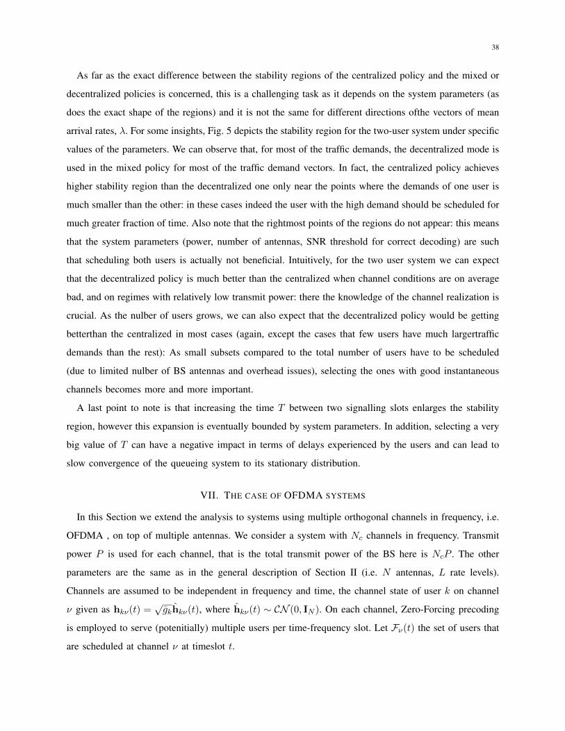
38

As far as the exact difference between the stability regions of the centralized policy and the mixed or

decentralized policies is concerned, this is a challenging task as it depends on the system parameters (as

does the exact shape of the regions) and it is not the same for different directions ofthe vectors of mean

arrival rates, λ. For some insights, Fig. 5 depicts the stability region for the two-user system under specific

values of the parameters. We can observe that, for most of the traffic demands, the decentralized mode is

used in the mixed policy for most of the traffic demand vectors. In fact, the centralized policy achieves

higher stability region than the decentralized one only near the points where the demands of one user is

much smaller than the other: in these cases indeed the user with the high demand should be scheduled for

much greater fraction of time. Also note that the rightmost points of the regions do not appear: this means

that the system parameters (power, number of antennas, SNR threshold for correct decoding) are such

that scheduling both users is actually not beneficial. Intuitively, for the two user system we can expect

that the decentralized policy is much better than the centralized when channel conditions are on average

bad, and on regimes with relatively low transmit power: there the knowledge of the channel realization is

crucial. As the nulber of users grows, we can also expect that the decentralized policy would be getting

betterthan the centralized in most cases (again, except the cases that few users have much largertraffic

demands than the rest): As small subsets compared to the total number of users have to be scheduled

(due to limited nulber of BS antennas and overhead issues), selecting the ones with good instantaneous

channels becomes more and more important.

A last point to note is that increasing the time T between two signalling slots enlarges the stability

region, however this expansion is eventually bounded by system parameters. In addition, selecting a very

big value of T can have a negative impact in terms of delays experienced by the users and can lead to

slow convergence of the queueing system to its stationary distribution.

VII. THE CASE OF OFDMA SYSTEMS

In this Section we extend the analysis to systems using multiple orthogonal channels in frequency, i.e.

OFDMA , on top of multiple antennas. We consider a system with Nc channels in frequency. Transmit

power P is used for each channel, that is the total transmit power of the BS here is NcP . The other

parameters are the same as in the general description of Section II (i.e. N antennas, L rate levels).

Channels are assumed to be independent in frequency and time, the channel state of user k on channel

ν given as hkν(t) =√gkhkν(t), where hkν(t) ∼ CN (0, IN ). On each channel, Zero-Forcing precoding

is employed to serve (potenitially) multiple users per time-frequency slot. Let Fν(t) the set of users that

are scheduled at channel ν at timeslot t.

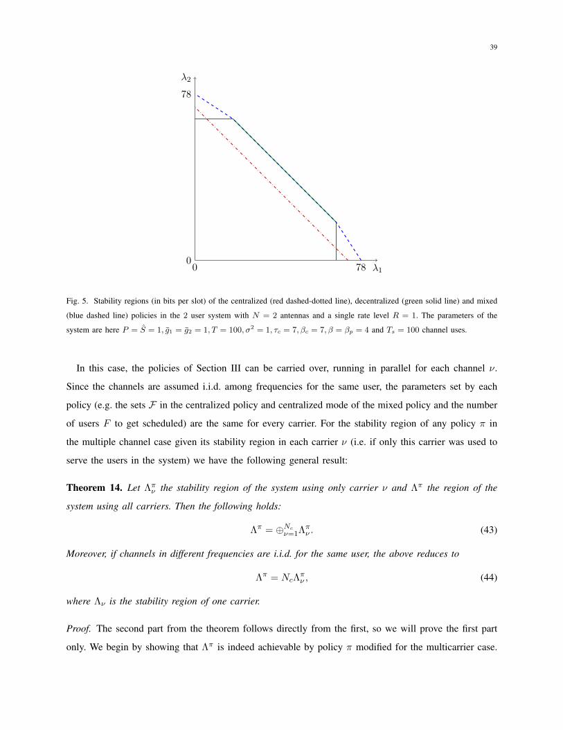
39

λ10 78

λ2

0

78

Fig. 5. Stability regions (in bits per slot) of the centralized (red dashed-dotted line), decentralized (green solid line) and mixed

(blue dashed line) policies in the 2 user system with N = 2 antennas and a single rate level R = 1. The parameters of the

system are here P = S = 1, g1 = g2 = 1, T = 100, σ2 = 1, τc = 7, βc = 7, β = βp = 4 and Ts = 100 channel uses.

In this case, the policies of Section III can be carried over, running in parallel for each channel ν.

Since the channels are assumed i.i.d. among frequencies for the same user, the parameters set by each

policy (e.g. the sets F in the centralized policy and centralized mode of the mixed policy and the number

of users F to get scheduled) are the same for every carrier. For the stability region of any policy π in

the multiple channel case given its stability region in each carrier ν (i.e. if only this carrier was used to

serve the users in the system) we have the following general result:

Theorem 14. Let Λπν the stability region of the system using only carrier ν and Λπ the region of the

system using all carriers. Then the following holds:

Λπ = ⊕Ncν=1Λπν . (43)

Moreover, if channels in different frequencies are i.i.d. for the same user, the above reduces to

Λπ = NcΛπν , (44)

where Λν is the stability region of one carrier.

Proof. The second part from the theorem follows directly from the first, so we will prove the first part

only. We begin by showing that Λπ is indeed achievable by policy π modified for the multicarrier case.

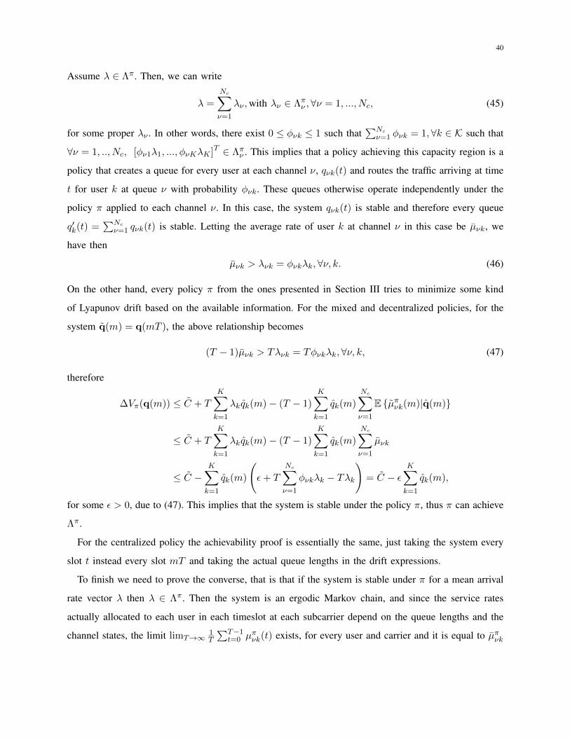
40

Assume λ ∈ Λπ. Then, we can write

λ =

Nc∑ν=1

λν ,with λν ∈ Λπν ,∀ν = 1, ..., Nc, (45)

for some proper λν . In other words, there exist 0 ≤ φνk ≤ 1 such that∑Nc

ν=1 φνk = 1,∀k ∈ K such that

∀ν = 1, .., Nc, [φν1λ1, ..., φνKλK ]T ∈ Λπν . This implies that a policy achieving this capacity region is a

policy that creates a queue for every user at each channel ν, qνk(t) and routes the traffic arriving at time

t for user k at queue ν with probability φνk. These queues otherwise operate independently under the

policy π applied to each channel ν. In this case, the system qνk(t) is stable and therefore every queue

q′k(t) =∑Nc

ν=1 qνk(t) is stable. Letting the average rate of user k at channel ν in this case be µνk, we

have then

µνk > λνk = φνkλk,∀ν, k. (46)

On the other hand, every policy π from the ones presented in Section III tries to minimize some kind

of Lyapunov drift based on the available information. For the mixed and decentralized policies, for the

system q(m) = q(mT ), the above relationship becomes

(T − 1)µνk > Tλνk = Tφνkλk,∀ν, k, (47)

therefore

∆Vπ(q(m)) ≤ C + T

K∑k=1

λkqk(m)− (T − 1)

K∑k=1

qk(m)

Nc∑ν=1

E {µπνk(m)|q(m)}

≤ C + T

K∑k=1

λkqk(m)− (T − 1)

K∑k=1

qk(m)

Nc∑ν=1

µνk

≤ C −K∑k=1

qk(m)

(ε+ T

Nc∑ν=1

φνkλk − Tλk

)= C − ε

K∑k=1

qk(m),

for some ε > 0, due to (47). This implies that the system is stable under the policy π, thus π can achieve

Λπ.

For the centralized policy the achievability proof is essentially the same, just taking the system every

slot t instead every slot mT and taking the actual queue lengths in the drift expressions.

To finish we need to prove the converse, that is that if the system is stable under π for a mean arrival

rate vector λ then λ ∈ Λπ. Then the system is an ergodic Markov chain, and since the service rates

actually allocated to each user in each timeslot at each subcarrier depend on the queue lengths and the

channel states, the limit limT→∞1T

∑T−1t=0 µπνk(t) exists, for every user and carrier and it is equal to µπνk

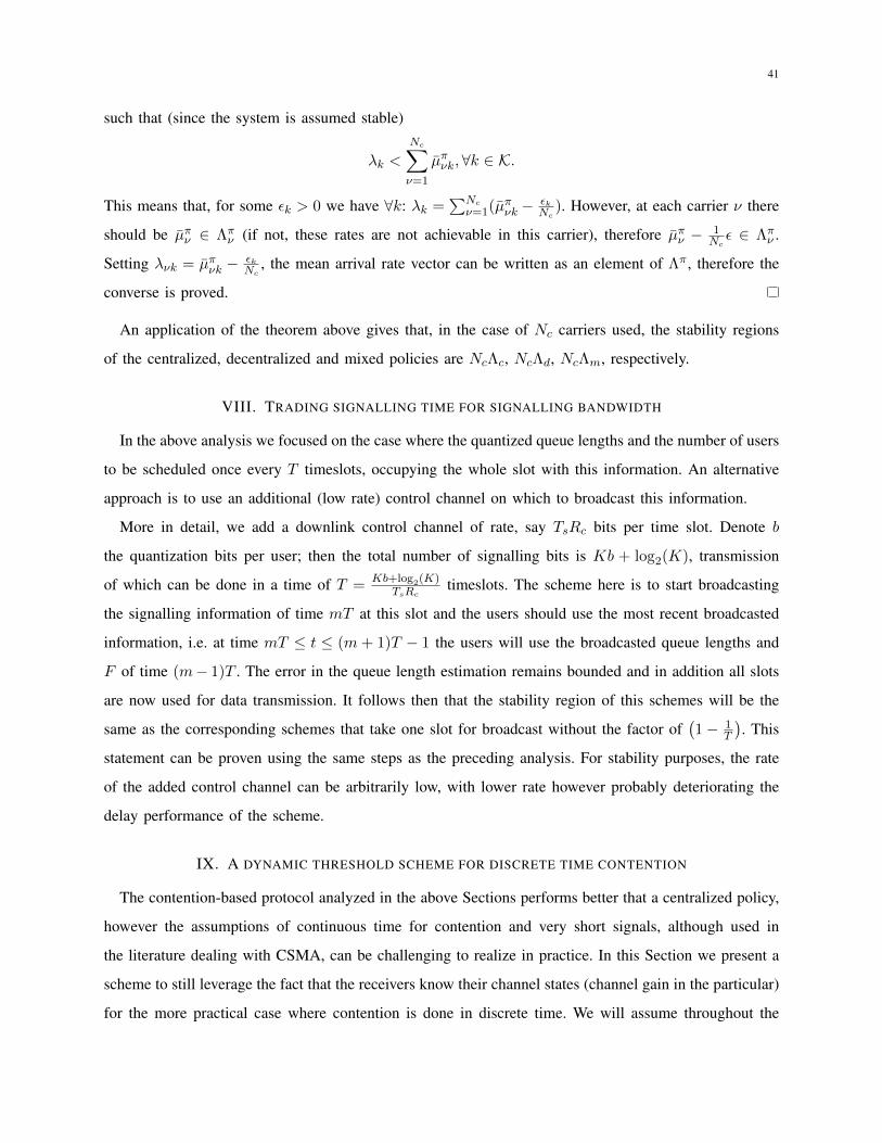
41

such that (since the system is assumed stable)

λk <

Nc∑ν=1

µπνk, ∀k ∈ K.

This means that, for some εk > 0 we have ∀k: λk =∑Nc

ν=1(µπνk −εkNc

). However, at each carrier ν there

should be µπν ∈ Λπν (if not, these rates are not achievable in this carrier), therefore µπν − 1Ncε ∈ Λπν .

Setting λνk = µπνk −εkNc

, the mean arrival rate vector can be written as an element of Λπ, therefore the

converse is proved.

An application of the theorem above gives that, in the case of Nc carriers used, the stability regions

of the centralized, decentralized and mixed policies are NcΛc, NcΛd, NcΛm, respectively.

VIII. TRADING SIGNALLING TIME FOR SIGNALLING BANDWIDTH

In the above analysis we focused on the case where the quantized queue lengths and the number of users

to be scheduled once every T timeslots, occupying the whole slot with this information. An alternative

approach is to use an additional (low rate) control channel on which to broadcast this information.

More in detail, we add a downlink control channel of rate, say TsRc bits per time slot. Denote b

the quantization bits per user; then the total number of signalling bits is Kb + log2(K), transmission

of which can be done in a time of T = Kb+log2(K)TsRc

timeslots. The scheme here is to start broadcasting

the signalling information of time mT at this slot and the users should use the most recent broadcasted

information, i.e. at time mT ≤ t ≤ (m+ 1)T − 1 the users will use the broadcasted queue lengths and

F of time (m− 1)T . The error in the queue length estimation remains bounded and in addition all slots

are now used for data transmission. It follows then that the stability region of this schemes will be the

same as the corresponding schemes that take one slot for broadcast without the factor of(1− 1

T

). This

statement can be proven using the same steps as the preceding analysis. For stability purposes, the rate

of the added control channel can be arbitrarily low, with lower rate however probably deteriorating the

delay performance of the scheme.

IX. A DYNAMIC THRESHOLD SCHEME FOR DISCRETE TIME CONTENTION

The contention-based protocol analyzed in the above Sections performs better that a centralized policy,

however the assumptions of continuous time for contention and very short signals, although used in

the literature dealing with CSMA, can be challenging to realize in practice. In this Section we present a

scheme to still leverage the fact that the receivers know their channel states (channel gain in the particular)

for the more practical case where contention is done in discrete time. We will assume throughout the

42

Section that the channels of the users are i.i.d. with hk(t) ∼ CN (0, IN ), ∀k ∈ {1, ..,K}. In practice

(where the users are in different distances from the BS), this can be achieved by appropriate power

control.

The main idea here is to have users with channel magnitude above a threshold train and get scheduled.

This threshold is updated dynamically by the BS, based on the state of the queues. We would like to

mention here that there is a rich literature concerning the idea of threshold-based feedback in single-input

single-output (SISO) systems in order to reduce the feedback overhead while selecting a ”good” user to

schedule. It was initiated in [34], [35] for sum-rate maximization without considering the queues of the

users. The recent work [36] addressed the problem of stability region expansion. Therein, the channel state

of the user with the largest queue is used as threshold. The above frameworks cannot be simply extended to

MIMO systems. In fact, in MIMO systems using ZF precoding (or in more general beamforming), the bit

rate of each user does not depend only on its channel conditions but also on the channel realization of the

other users that get served simultaneously, making the problem more challenging. Finally, authors in [37]

employ similar ideas for a multiuser MIMO system where the receivers employ ZF. Apart from focusing

on the receivers and not the precoding at the transmitter, this work addresses sum rate maximization, so

the traffic processes of the users are not taken into account.

A. Protocol Description

More in detail, the BS uses slots 0, T, 2T, ..,mT, ... for signaling and setting the control parameters to

be used for the next T−1 slots. T is a (positive and possibly high) constant whose role in the performance

of the algorithm will be examined in the next subsection. There are therefore two distinct phases:

1) Broadcast phase (t=0,T,2T,...): At slot mT the BS broadcasts IDs of the K(m) users with the biggest

queue lengths (the set K(m)) ordered by decreasing queue length, the preferred number of users to be

served F (m) and the threshold G(m), given as the solution of (51) that follows.

2) Uplink Training phase in each time slot: In all T − 1 slots (i.e. between slots mT and (m+ 1)T ),

the user selection for uplink training is done as follows. A portion of the time slot is reserved to receive

information from the users in K(m) about their channels. This portion of time is divided into minislots of

total number equal to the number of users in K(m). In each minislot (which lasts for one channel use), a

user sends a signal (e.g. 1 bit signal) if its channel gain is above G(m) and does nothing otherwise. The

minislots are shared among the users in K(m) in a TDMA manner according to the ordering broadcasted

by the BS at slot mT . The procedure stops in the following cases:

i. When F (m) users with channel above the threshold are found. In this case these users get scheduled

43

for uplink training and the user selection period lasts for L(G(m), F (m)) channel uses. These F (m)

will send then their uplink training sequences that will last βF (m) channel uses. The remaining time

in the current time slot is then used for data transmission (we will see that even with this additional

signaling the performance of this algorithm is better than the baseline user selection algorithm).

ii. When all users in K have sent the 1 bit signal (as above) and U ≤ F (m) users have signaled that

their channel gain is above the threshold. These U users will then get scheduled for training and

transmission and the user selection period lasts for K channel uses. These U users will then send

their training sequences (i.e. βU channel uses are used for uplink training). The remaining of the

time slot is then used for data transmission.

The parameters to be optimized here are (i) the ordering of the users, (ii) the candidate users in the set

K(m),(iii) the number of users, F (m), to get scheduled and (iv) the threshold for the channel magnitudes,

G, which should be in general a function of the queue lengths, F (m) and K(m).

Under the setting of i.i.d. channels for the users, they will be ordered according to their queue lengths

at (the beginning of) timeslot mT , with the user with the largest queue first. This implies that the set of

candidate users consists in the K(m) users with the biggest queue lengths.

We now turn to the impact of the threshold G. The probability that the channel magnitude of a user

is above this threshold is given as

p(G) = P{gk(t) > G} = 1− γ(G;N)

Γ(N)= 1−

∫ +∞

G

xN−1e−x

Γ(N)dx. (48)

The above follows from the fact that since hk(t) ∼ CN (0, IN ), the quantity 2 ||hk(t)||2 follows a chi-

squared distribution with 2N degrees of freedom. In addition, let

rd(F,G) = E{rk(t)

∣∣∣∣F, gk(t) > G

}be the mean rate in bits per channel use that user k gets if his channel magnitude is above the threshold

and F users are scheduled in total. These can be calculated using the results of Section IV-A.

Intuitively, smaller threshold will cause the signalling phase to end faster, however users with worse

channel condition may be selected. Assume a user ordering {k(1), k(2)..., k(K)} such that qk(1)(mT ) ≥

qk(2)(mT ) ≥ ... ≥ qk(K)(mT ). Then, defining

M(i,m,U) =

min{U−2,i−1}∑j=max {0,U−1−m+i}

(i− 1

j

)(m− i− 1

U − (j − 2)

),

we have the following

44

Lemma 15. The mean rate, µk(i)(F, K,G) the i-th user in the ordering gets if the threshold is G and

the BS signalled for F users out of the K users with the bigguest queue lengths to be scheduled is, for

i ≤ K:

µi(1, K, G) = [Ts − (βp + βci+ β)]+p(G)(1− p(g∗))i−1rd(F,G) (49)

for F (m) = 1 and

µi(F, K,G) = rd(F,G) [Ts − βp − βci− βF ]+ pF (G)(1− p(G))i−F1{F≤i}

+ rd(F,G)pF (G)

K∑m′=max[F,i+1]

[Ts − βp − βcm′ − βF

]+M(i,m′, F )(1− p(G))m

′−F

+

F−1∑F ′=1

(K − 1

F ′ − 1

)[Ts − βp − K − βF ′]+pF

′(G)(1− p(G))K−F

′rd(F

′, G), (50)

for 2 ≤ F (m) ≤ Fmax. In addition, µk(i)(F, K,G) = 0 for i > K.

Proof. Please refer to Appendix C for the proof.

The expected weight for F (m) = F and threshold for the channel gain set to g∗ then is given as

E

{K∑k=1

qk(mT )µk(t)zk(t)

∣∣∣∣F, K,G}

=

K∑i=1

qk(i)(mT )µi(F, K,G).

From the above, the BS sets at slot mT the parameters F (m), g∗(m) to be used in slots mT+1, ...,mT+

T − 1 as a solution to the following optimization problem:

{F (m), K(m), G(m)} = arg max1≤F≤Fmax,1≤K≤K,G∈G

{K∑i=1

qk(i)(mT )µi(F, K,G)

}(51)

where G denotes the set of possible thresholds for the channel magnitude. The stability region achieved

by this protocol is then the following:

Theorem 16. The stability region of the threshold-based scheme when signaling is done every T slots is

Λthr(T ) =

(1− 1

T

)CHF∈{1,..,Fmax},K={1,..,K},G∈G

{Λ′(F, K,G)

},

where Λ′(F, K,G) is the convex hull of all points in RK resulting from all possible permutations of the

numbers µi(F, K,G).

The proof of the theorem is along the lines of the other proofs in this paper and thus is omitted.

45

B. Simulation Results

In order to illustrate the impact of the threshold-based in the stability region of the system, we simulated

a single cell system where the BS uses N = 4 antennas to serve K = 10 users. A single modulation and

coding scheme with a rate of R bits per channel use if the SNR of a scheduled user exceeds S is assumed.

Specifically, we set R = 1 bit per channel use. Each user has Poisson traffic with different average arrival

rates as λK := λ and λk−1 = 1.05λk: we parametrize the mean arrival rates by the smallest one and see

how the system behaves as this smallest rate varies. That means that the mean arrival rate vector is

λk = 1.0510−kλ,∀k ∈ {1, .., 10}. (52)

For simplicity, a threshold rule, where the threshold for the channel gain depends only on the preferred

number F of users to be served and threshold G = FSP is used. The reason for choosing this is that if

the channel gain of a user is smaller and F − 1 other users are served then the rate of this user will be

zero. We set the slot duration to be Ts = 1000 channel uses, and overheads for contention, downlink

pilot and uplink pilot length per user βc = 1, βp = 50 and β = 100 channel uses, respectively. The

rate for signalling is set to R0 = 0.2 bits per channel use. We assume that P = S = 1, that is the total

transmit power and the SNR threshold for correct decoding are at the same level of the noise floor.

We simulated the system under the centralized policy, as well as under the threshold-based policy

for different values of signalling period T and λ, each simulation lasting 106 timeslots. Notice that the

decentralized policies, described in the previous sections, achieve obviously better performance than the

centralized and threshold based policies. In order to illustrate the stability performance, we present in

Figure 6 the average total queue lengths, i.e. the quantity 1106

∑106−1t=0

∑Kk=1 qk(t). The point where the

system becomes unstable is the point where the total average queue length begins to increase very steeply.

We can see in the figure that, indeed, by selecting the signalling period T high enough, the threshold-

based algorithm outperforms the baseline centralized policy. Notice here that under the setting regarding

the physical layer, the total average service rate at each slot given that users with Pgk(t)/F > S are

scheduled can be at most 805, 1287, 1262, 954 if F = 1, 2, 3, 4 users are scheduled, respectively. The

average total number of incoming bits is 12.57λ, therefore the proposed schemes achieve a good fraction

of the biggest traffic achievable under our signalling constraints. As compared to the centralized policy,

the gain is around 20%. In addition, the bigger the signalling period T is, the bigger stability region

is achievable. Notice, however, that when T takes very high values, the increase in the stability region

from increasing T further becomes negligible. This can be interpreted theoretically, using the result in

Theorem 16 since the convex hull is multiplied by the(1− 1

T

)term.

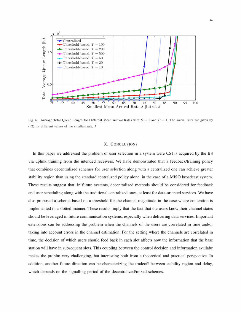
46

30 35 40 45 50 55 60 65 70 75 80 85 90 95 1000

0.5

1

1.5

2x 10

5

Smallest Mean Arrival Rate λ [bit/slot]

Total

Average

Queu

eLen

gth[bit]

CentralizedThreshold-based, T = 100

Threshold-based, T = 200

Threshold-based, T = 500

Threshold-based, T = 50

Threshold-based, T = 20

Threshold-based, T = 10

Fig. 6. Average Total Queue Length for Different Mean Arrival Rates with S = 1 and P = 1. The arrival rates are given by

(52) for different values of the smallest rate, λ.

X. CONCLUSIONS

In this paper we addressed the problem of user selection in a system were CSI is acquired by the BS

via uplink training from the intended receivers. We have demonstrated that a feedback/training policy

that combines decentralized schemes for user selection along with a centralized one can achieve greater

stability region than using the standard centralized policy alone, in the case of a MISO broadcast system.

These results suggest that, in future systems, decentralized methods should be considered for feedback

and user scheduling along with the traditional centralized ones, at least for data-oriented services. We have

also proposed a scheme based on a threshold for the channel magnitude in the case where contention is

implemented in a slotted manner. These results imply that the fact that the users know their channel states

should be leveraged in future communication systems, especially when delivering data services. Important

extensions can be addressing the problem when the channels of the users are correlated in time and/or

taking into account errors in the channel estimation. For the setting where the channels are correlated in

time, the decision of which users should feed back in each slot affects now the information that the base

station will have in subsequent slots. This coupling between the control decision and information availabe

makes the problm very challenging, but interesting both from a theoretical and practical perspective. In

addition, another future direction can be characterizing the tradeoff between stability region and delay,

which depends on the signalling period of the decentralized/mixed schemes.

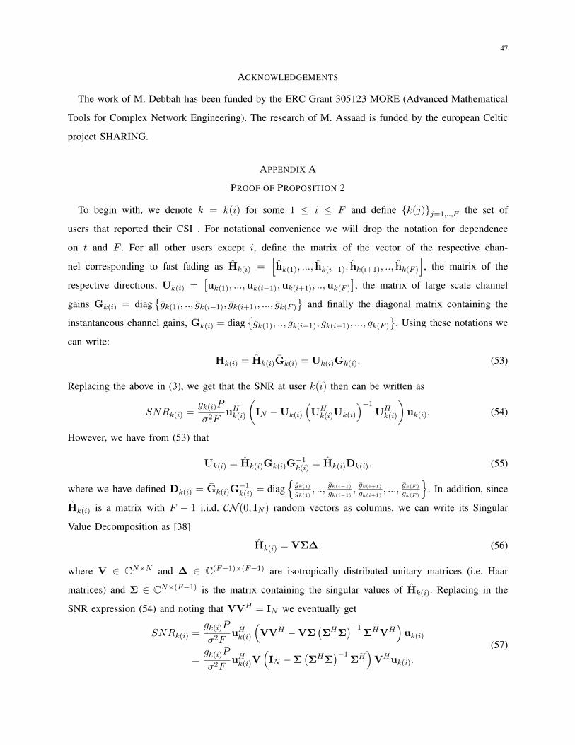
47

ACKNOWLEDGEMENTS

The work of M. Debbah has been funded by the ERC Grant 305123 MORE (Advanced Mathematical

Tools for Complex Network Engineering). The research of M. Assaad is funded by the european Celtic

project SHARING.

APPENDIX A

PROOF OF PROPOSITION 2

To begin with, we denote k = k(i) for some 1 ≤ i ≤ F and define {k(j)}j=1,..,F the set of

users that reported their CSI . For notational convenience we will drop the notation for dependence

on t and F . For all other users except i, define the matrix of the vector of the respective chan-

nel corresponding to fast fading as Hk(i) =[hk(1), ..., hk(i−1), hk(i+1), .., hk(F )

], the matrix of the

respective directions, Uk(i) =[uk(1), ...,uk(i−1),uk(i+1), ..,uk(F )

], the matrix of large scale channel

gains Gk(i) = diag{gk(1), .., gk(i−1), gk(i+1), ..., gk(F )

}and finally the diagonal matrix containing the

instantaneous channel gains, Gk(i) = diag{gk(1), .., gk(i−1), gk(i+1), ..., gk(F )

}. Using these notations we

can write:

Hk(i) = Hk(i)Gk(i) = Uk(i)Gk(i). (53)

Replacing the above in (3), we get that the SNR at user k(i) then can be written as

SNRk(i) =gk(i)P

σ2FuHk(i)

(IN −Uk(i)

(UHk(i)Uk(i)

)−1UHk(i)

)uk(i). (54)

However, we have from (53) that

Uk(i) = Hk(i)Gk(i)G−1k(i) = Hk(i)Dk(i), (55)

where we have defined Dk(i) = Gk(i)G−1k(i) = diag

{gk(1)gk(1)

, ..,gk(i−1)

gk(i−1),gk(i+1)

gk(i+1), ...,

gk(F )

gk(F )

}. In addition, since

Hk(i) is a matrix with F − 1 i.i.d. CN (0, IN ) random vectors as columns, we can write its Singular

Value Decomposition as [38]

Hk(i) = VΣ∆, (56)

where V ∈ CN×N and ∆ ∈ C(F−1)×(F−1) are isotropically distributed unitary matrices (i.e. Haar

matrices) and Σ ∈ CN×(F−1) is the matrix containing the singular values of Hk(i). Replacing in the

SNR expression (54) and noting that VVH = IN we eventually get

SNRk(i) =gk(i)P

σ2FuHk(i)

(VVH −VΣ

(ΣHΣ

)−1ΣHVH

)uk(i)

=gk(i)P

σ2FuHk(i)V

(IN −Σ

(ΣHΣ

)−1ΣH)

VHuk(i).

(57)

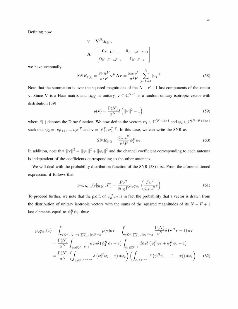
48

Defining now

v = VHuk(i),

A =

0F−1,F−1 0F−1,N−F+1

0N−F+1,F−1 IN−F+1

we have eventually

SNRk(i) =gk(i)P

σ2FvHAv =

gk(i)P

σ2F

N∑j=F+1

|uj |2. (58)

Note that the summation is over the squared magnitudes of the N −F + 1 last components of the vector

v. Since V is a Haar matrix and uk(i) is unitary, v ∈ CN×1 is a random unitary isotropic vector with

distribution [39]

p(v) =Γ(N)

πNδ(||v||2 − 1

), (59)

where δ(.) denotes the Dirac function. We now define the vectors ψ1 ∈ C(F−1)×1 and ψ2 ∈ C(N−F+1)×1

such that ψ2 = [vF+1, ..., vN ]T and v = [ψT1 , ψT2 ]T . In this case, we can write the SNR as

SNRk(i) =gk(i)P

σ2FψH2 ψ2. (60)

In addition, note that ||v||2 = ||ψ1||2 + ||ψ2||2 and the channel coefficient corresponding to each antenna

is independent of the coefficients corresponding to the other antennas.

We will deal with the probability distribution function of the SNR (58) first. From the aforementioned

expression, if follows that

pSNRk(i)(s|gk(i), F ) =Fσ2

gk(i)PpψH2 ψ2

(Fσ2

gk(i)Ps

)(61)

To proceed further, we note that the p.d.f. of ψH2 ψ2 is in fact the probability that a vector is drawn from

the distribution of unitary isotropic vectors with the sums of the squared magnitudes of its N − F + 1

last elements equal to ψH2 ψ2, thus:

pψH2 ψ2(x) =

∫v∈CN :||v||=1,

∑Nk=F |vk|2=x

p(v)dv =

∫v∈CN :

∑Nk=F |vk|2=x

Γ(N)

πNδ(vHv − 1

)dv

=Γ(N)

πN

∫ψ2∈CN−F+1

dψ2δ(ψH2 ψ2 − x

) ∫ψ1∈CF−1

dψ1δ(ψH1 ψ1 + ψH2 ψ2 − 1

)=

Γ(N)

πN

(∫ψ2∈CN−F+1

δ(ψH2 ψ2 − x

)dψ2

)(∫ψ1∈CF−1

δ(ψH1 ψ1 − (1− x)

)dψ1

)(62)

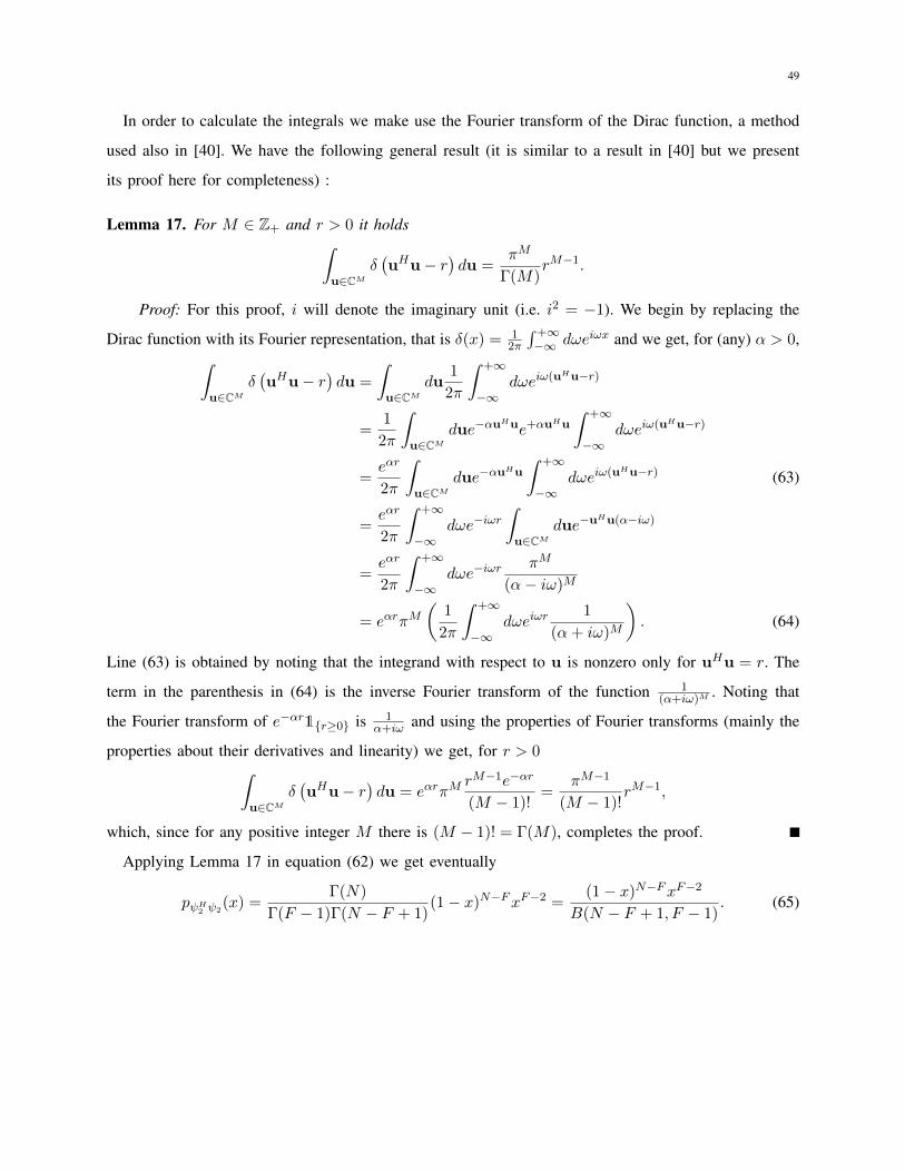
49

In order to calculate the integrals we make use the Fourier transform of the Dirac function, a method

used also in [40]. We have the following general result (it is similar to a result in [40] but we present

its proof here for completeness) :

Lemma 17. For M ∈ Z+ and r > 0 it holds∫u∈CM

δ(uHu− r

)du =

πM

Γ(M)rM−1.

Proof: For this proof, i will denote the imaginary unit (i.e. i2 = −1). We begin by replacing the

Dirac function with its Fourier representation, that is δ(x) = 12π

∫ +∞−∞ dωeiωx and we get, for (any) α > 0,∫

u∈CMδ(uHu− r

)du =

∫u∈CM

du1

2π

∫ +∞

−∞dωeiω(uHu−r)

=1

2π

∫u∈CM

due−αuHue+αuHu

∫ +∞

−∞dωeiω(uHu−r)

=eαr

2π

∫u∈CM

due−αuHu

∫ +∞

−∞dωeiω(uHu−r) (63)

=eαr

2π

∫ +∞

−∞dωe−iωr

∫u∈CM

due−uHu(α−iω)

=eαr

2π

∫ +∞

−∞dωe−iωr

πM

(α− iω)M

= eαrπM(

1

2π

∫ +∞

−∞dωeiωr

1

(α+ iω)M

). (64)

Line (63) is obtained by noting that the integrand with respect to u is nonzero only for uHu = r. The

term in the parenthesis in (64) is the inverse Fourier transform of the function 1(α+iω)M . Noting that

the Fourier transform of e−αr1{r≥0} is 1α+iω and using the properties of Fourier transforms (mainly the

properties about their derivatives and linearity) we get, for r > 0∫u∈CM

δ(uHu− r

)du = eαrπM

rM−1e−αr

(M − 1)!=

πM−1

(M − 1)!rM−1,

which, since for any positive integer M there is (M − 1)! = Γ(M), completes the proof.

Applying Lemma 17 in equation (62) we get eventually

pψH2 ψ2(x) =

Γ(N)

Γ(F − 1)Γ(N − F + 1)(1− x)N−FxF−2 =

(1− x)N−FxF−2

B(N − F + 1, F − 1). (65)

50

Using (61) and replacing with (65) we have

P{SNRk(i) > S|gk(i), F

}=

∫ Pgk(i)

σ2F

SpSNRk(i)(s|gk(i), F )ds

=

∫ Pgk(i)

σ2F

S

Fσ2

gk(i)PpψH2 ψ2

(Fσ2

gk(i)Ps

)ds

=

∫ 1

Fσ2

Pgk(i)SpψH2 ψ2

(x)dx

=1

B(N − F + 1, F − 1)

∫ 1

Fσ2

Pgk(i)S

(1− x)N−FxF−2dx,

which is the stated result.

APPENDIX B

PROOF OF LEMMA 5

From the evolution equation for the sampled queue lengths we have

q2k(m+ 1) =

(qk(m) +

T−1∑t=0

ak(mT + t)−T−1∑t=1

zk(mT + t)µk(mT + t)+

T−1∑t=1

yk(mT + t)

)2

≤

(qk(m) +

T−1∑t=0

ak(mT + t)−T−1∑t=1

zk(mT + t)µk(mT + t)

)2

= q2k(m) +

(T−1∑t=0

ak(mT + t)

)2

+

(T−1∑t=1

zk(mT + t)µk(mT + t)

)2

+ 2qk(m)

T−1∑t=0

ak(mT + t)− 2qk(m)

T−1∑t=1

zk(mT + t)µk(mT + t)

≤ q2k(m) + T 2A2

max + (T − 1)2R2L

− 2qk(m)

T−1∑t=0

ak(mT + t) + 2qk(m)

T−1∑t=1

zk(mT + t)µk(mT + t).

51

From the above, setting B = K(T 2A2max + (T − 1)2R2

L) and taking expectations it follows that

∆V (q(m)) ≤ B + E

{K∑k=1

2qk(m)

T−1∑t=0

ak(mT + t)|qk(m)

}

− E

{K∑k=1

2qk(m)

T−1∑t=1

zk(mT + t)µk(mT + t)|qk(m)

}

= B + 2

K∑k=1

qk(m)

T−1∑t=0

E{ak(mT + t)}

− 2

K∑k=1

qk(m)

T−1∑t=1

E{zk(mT + t)µk(mT + t)|q(m)}

= B + 2T

K∑k=1

qk(m)λk

− 2

K∑k=1

qk(m)

T−1∑t=1

E{zk(mT + t)µk(mT + t)|q(m)}

Where the last equality follows from the fact that the arrival processes are i.i.d. in time and independent

of anything else. Moreover, we have that the schedule zk(mT + t) and the rate of the user in the slot

µk(mT + t) depend only on the queue length vector q(m) and the realizations of the channels and

not on the time index. This implies that the product zk(mT + t)µk(mT + t) has the same distribution

for every slot between mT + 1 ≤ τ ≤ m(T + 1). Defining µk(m) as this final rate (including the

scheduling decision) user k gets, for a given scheme it is as if we have (T − 1) independent copies

of this random variable (with probability distribution over the probability distribution of the channels),

hence the statement follows.

APPENDIX C

PROOF OF LEMMA 15

Proof of equation (49): Notice that here only one user is to be scheduled (since F (m) = 1). This

means that the i-th user in the ordering gets scheduled if (i) his channel magnitude is above the threshold

and (ii) the channel magnitudes of the i− 1 users before him are below the threshold. In addition, if this

user is scheduled the contention period stops right after, i.e. lasts for i minislots.

Proof of equation (50): We now deal with the case where 2 ≤ F (m) = F ≤ Fmax. The mean rate of

52

the i-th user in the ordering can be written as follows:

µk(i)(F, K,G) =P {F users above G, k(i) ∈ F}E{µk(i)|F above G, k(i) ∈ F

}+

F−1∑F ′=1

P{F ′ users above G, k(i) ∈ F

}E{µk(i)|F ′ aboveG, k(i) ∈ F

}

:= µi(F ) +

F−1∑F ′=1

µi(F′).

(66)

For the rest of the proof, we will denote the event that user k(i) is scheduled as k(i) ∈ F . For the first

term of the above equation, which corresponds to the event that F (m) = F users get scheduled in the

end, we have

µi(F ) =

K∑m=F

P {M = m, k(i) ∈ F , |F| = F} [Ts − (βp + βF + βcm)]+E{rk(i)(t)

∣∣∣∣F, gk(i)(t) > G

},

(67)

where M denotes the duration of the contention period (i.e. how many minislots are used till F users

are found with the channel magnitude above the threshold). Since k(i) should be in the set of users that

are scheduled, the contention period should not stop before his minislot, that is

P {M = m, k(i) ∈ F , |F| = F} = 0, ∀0 ≤ m < i.

In addition, we should also have m ≥ F . Combined with the above, it implies that m ≥ max{F, i}.

Tanking also into account that, by definition E{rk(i)(t)

∣∣∣∣F, gk(i)(t) > G

}= rd(F,G), the sum in (67)

can be then rewritten as follows:

µi(F ) =1{i≥F}[Ts − (βp + βF + i]+P {M = i, k(i) ∈ F , |F| = F} rd(F,G)

+

K∑m=max{F,i+1}

P {M = m, k(i) ∈ F , |F| = F} [Ts − (βp + βF + βcm)]+rd(F,G),(68)

The first term of (68) corresponds to the case where k(i) is the last user to send the signal that its

channel gain is greater than G. In this case, exactly F − 1 out of the i − 1 previou users must have

channel gain above G, therefore

P{M = i, k(i) ∈ F ,|F| = F

}=

(i− 1

F − 1

)pF (G)(1− p(G))i−F (69)

For the second term of (68), we note that the event in the probability is equivalent to the union of

events where (i) the channel magnitude of user k(i) is above G (ii)the channel magnitude of user k(m)

53

is above G and (iii) f users with lower order than i, that is between and including k(1) and k(i−1) and

F − f − 2 between and including k(i+ 1) and k(m− 1) have channel magnitudes above the threshold,

for all values of f . The values f is allowed to take should satisfy the following properties:

0 ≤ f ≤ i− 1

f ≤ F − 2

F − (f + 2) ≤ m− 1− i =⇒ f ≥ F − 1− (m− i).

(70)

The first condition in (70) comes from the fact that the number of users before the i-th user is i − 1,

the second from the fact that since k(i) and k(m) should both be scheduled, not more than F − 2 users

higher in the ranking of k(i) should have channel magnitudes above the threshold and the third because

there are left m− i users in the ranking between, and not including users k(i) and k(m) . We thus have

P {M = m, k(i) ∈ F , |F| = F} = p2(G)

min{F−2,i−1}∑f=max{0,F−1−m+i}

P{f in {k(1), ..., k(i− 1) above G,

F − (f + 2) in {k(i+ 1), ..., k(m− 1) above G},

which, since the channels are i.i.d. among users reduces to

P {M = m, k(i) ∈ F , |F| = F} =

p2(G)

min{F−2,i−1}∑f=max{0,F−1−m+i}

P{f out of i− 1 above G

}P{F − (f + 2) out of m− 1− i above G

}.

The event in the first term inside the sum happens in(i−1f

)possible ways with probability pf (G)(1 −

p(G))i−1−f each, while the event in the second term happens in(m−1−iF−(f+2)

)ways, with probability

pF−(f+2)(G)(1− p(G))m−i−(F−(f+1)) each. Replacing and taking into account that F ≤ m (all F users

should get scheduled) and we get eventually

P {M = m, k(i) ∈ F , |F| = F} = p(G)F (1− p(G))m−Fmin{F,i}−1∑

f=max{0,F−1−m+i}

(i− 1

f

)(m− 1− iF − (f + 2)

),

for max{F, i+ 1} ≤ m ≤ K

(71)

We now turn to the second term of (66), i.e. the sum∑F−1

F ′=1 µi(F′). This is in fact due to the probability

that less than F users can have channel magnitude above the threshold. The event that exactly F ′ < F

users have channel magnitude above the threshold and user k(i) is scheduled is the same as user k(i)

having channel magnitude over the threshold and exactly F ′−1 out of the remaining K−1 users do. This

54

event can happen in(K−1F ′−1

)combinations, each having a probability of p(g∗)pF

′−1(g∗)(1− p(g∗))K−F ′ .

On the other hand, if less than F users are above the threshold then all K minislots are used, therefore

the contention period lasts for K channel uses. Finally, F ′ users participate in the uplink training. We

then have

µi(F′) =

(K − 1

F ′ − 1

)pF′(G)(1− p(G))K−F

′[Ts − (βp + βcK + βF ′)]+E

{rk(i)(t)

∣∣∣∣F ′, gk(i)(t) > G

}.

(72)

The result follows combining (66) with (67), (68), (69), (71) and (72).

REFERENCES

[1] G. Foschini and M. Gans, “On limits of wireless communications in a fading environment when using multiple antennas,”

Wireless Personal Communications, vol. 6, no. 3, pp. 311–335, 1998.

[2] D. Gesbert, M. Kountouris, R. Heath, C.-B. Chae, and T. Salzer, “Shifting the MIMO paradigm,” IEEE Signal Process.

Mag., vol. 24, no. 5, pp. 36–46, 2007.

[3] H. Weingarten, Y. Steinberg, and S. Shamai, “The Capacity Region of the Gaussian Multiple-Input Multiple-Output

Broadcast Channel,” IIEEE Trans. Info. Theory, vol. 52, no. 9, pp. 3936–3964, Sept. 2006.

[4] D. Love, R. Heath, V. Lau, D. Gesbert, B. Rao, and M. Andrews, “An overview of limited feedback in wireless

communication systems,” IEEE J. Sel. Areas Commun., vol. 26, no. 8, pp. 1341 –1365, Oct. 2008.

[5] G. Caire, N. Jindal, M. Kobayashi, and N. Ravindran, “Multiuser mimo achievable rates with downlink training and channel

state feedback,” IEEE Transactions on Information Theory, vol. 56, no. 6, Jun. 2010.

[6] M. Kobayashi, N. Jindal, and G. Caire, “Training and Feedback Optimization for Multiuser MIMO Downlink,” IEEE

Trans. Commun., vol. 59, no. 8, pp. 2228–2240, Aug.t 2011.

[7] L. Song, Z. Han, Z. Zhang, and B. Jiao, “Non-cooperative feedback-rate control game for channel state information in

wireless networks,” IEEE Journal on Selected Areas in Communications, vol. 30, no. 1, pp. 188 –197, Jan. 2012.

[8] H. Boche and M. Wiczanowski, “The interplay of link layer and physical layer under MIMO enhancement: benefits and

challenges,” IEEE Wireless Commun. Mag., vol. 13, no. 4, pp. 48–55, Aug. 2006.

[9] ——, “Optimization-Theoretic Analysis of Stability-Optimal Transmission Policy for Multiple-Antenna Multiple-Access

Channel,” IEEE Trans. Signal Process., vol. 55, no. 6, pp. 2688–2702, Jun. 2007.

[10] C. Swannack, E. Uysal-Biyikoglu, and G. Wornell, “Low Complexity Multiuser Scheduling for Maximizing Throughput

in the MIMO Broadcast Channel,” in Allerton Conference on Communications, Control, and Computing, Monticello, IL,

USA, 2004.

[11] M. Kobayashi and G. Caire, “An iterative water-filling algorithm for maximum weighted sum-rate of Gaussian MIMO-BC,”

IEEE J. Sel. Areas Commun., vol. 24, no. 8, pp. 1640–1646, Aug. 2006.

[12] C. Wang and R. Murch, “Optimal downlink multi-user MIMO cross-layer scheduling using HOL packet waiting time,”

IEEE Transactions on Wireless Communications, vol. 5, no. 10, pp. 2856–2862, Oct. 2006.

[13] M. Kobayashi, G. Caire, and D. Gesbert, “Transmit diversity versus opportunistic beamforming in data packet mobile

downlink transmission,” IEEE Transactions on Communications,, vol. 55, no. 1, pp. 151–157, Jan. 2007.

[14] M. Kobayashi and G. Caire, “Joint Beamforming and Scheduling for a Multi-Antenna Downlink with Imperfect Transmitter

Channel Knowledge,” IEEE J. Sel. Areas Commun., vol. 25, no. 7, pp. 1468–1477, Sep. 2007.

55

[15] K. Huang and V. Lau, “Stability and delay of zero-forcing SDMA with limited feedback,” IEEE Trans. Inf. Theory, vol. 58,

no. 10, pp. 6499–6514, Oct. 2012.

[16] J. Jose, A. Ashikhmin, P. Whiting, and S. Vishwanath, “Channel Estimation and Linear Precoding in Multiuser Multiple-

Antenna TDD Systems,” IEEE Transactions on Vehicular Technology, vol. 60, no. 5, pp. 2102–2116, Jun. 2011.

[17] T. Yoo and A. Goldsmith, “On the optimality of multiantenna broadcast scheduling using zero-forcing beamforming,” IEEE

Journal on Selected Areas in Communications, vol. 24, no. 3, pp. 528–541, Mar. 2006.

[18] S. Sesia, I. Toufik, and M. Baker, LTE, The UMTS Long Term Evolution: From Theory to Practice. Wiley, 2009.

[19] S. Lakshminarayana, B. Li, M. Assaad, A. Eryilmaz, and M. Debbah, “A fast-CSMA based distributed scheduling algorithm

under SINR model,” in IEEE nternational Symposeum on Information Theory (ISIT), Princeton, NJ, USA, 2012, pp. 1598–

1602.

[20] M. Karaca, E. Ekici, and O. Ercetin, “Throughput-optimal distributed algorithm for wlans over fading channels,” ArXiv

e-prints, vol. abs/1301.2750, 2013.

[21] B. Li and A. Eryilmaz, “Distributed channel probing for efficient transmission scheduling over wireless fading channels,”

in IEEE International Conference on Computer Communications (INFOCOM), Mar. 2012, pp. 3026 –3030.

[22] A. Eryilmaz, R. Srikant, and J. R. Perkins, “Stable scheduling policies for fading wireless channels,” IEEE/ACM

Transactions on Networking, vol. 13, no. 2, pp. 411–424, Apr. 2005.

[23] K. Kar, X. Luo, and S. Sarkar, “Throughput-optimal scheduling in multichannel access point networks under infrequent

channel measurements,” IEEE Transactions on Wireless Communications, vol. 7, no. 7, pp. 2619–2629, Jul. 2008.

[24] J. Hoydis, M. Kobayashi, and M. Debbah, “Optimal Channel Training in Uplink Network MIMO Systems,” IEEE

Transactions on Signal Processing, vol. 59, no. 6, pp. 2824–2833, Jun. 2011.

[25] M. J. Neely, “Stochastic network optimization with application to communication and queueing systems,” Synthesis Lectures

on Communication Networks, vol. 3, no. 1, pp. 1–211, 2010.

[26] L. Tassiulas and A. Ephremides, “Stability properties of constrained queueing systems and scheduling policies for maximum

throughput in multihop radio networks,” IEEE Trans. Autom. Control, vol. 37, no. 12, pp. 1936 –1948, Dec. 1992.

[27] A. L. Stolyar, “Maxweight Scheduling in a Generalized Switch: State Space Collapse and Workload Minimization in Heavy

Traffic,” The Annals of Applied Probability, vol. 14, no. 1, pp. 1–53, 2004.

[28] P. Chaporkar, A. Proutiere, H. Asnani, and A. Karandikar, “Scheduling with limited information in wireless systems,” in

ACM International Symposium on Mobile Ad Hoc Networking and Computing (MobiHoc), 2009, pp. 75–84.

[29] T. Marzetta, “Noncooperative cellular wireless with unlimited numbers of base station antennas,” IEEE Transactions on

Wireless Communications, vol. 9, no. 11, pp. 3590–3600, Sep. 2010.

[30] D. Shah and J. Shin, “Randomized scheduling algorithm for queueing networks.” Annals of Applied Probability, vol. 22,

no. 1, pp. 128–171, 2012.

[31] S. S. Nam, H.-C. Yang, M.-S. Alouini, and D. I. Kim, “Exact capture probability analysis of GSC receivers over i.n.d.

rayleigh fading channels,” in IEEE International Symposium on Information Theory (ISIT), 2013, July 2013, pp. 56–60.

[32] ——, “Technical report: An MGF-based unified framework to determine the joint statistics of partial sums of ordered i.n.d.

random variables,” ArXiV e-prints, vol. abs/1307.8199, 2013.

[33] N. Jindal, J. Andrews, and S. Weber, “Multi-antenna communication in ad hoc networks: Achieving mimo gains with simo

transmission,” IEEE Transactions on Communications, vol. 59, no. 2, pp. 529–540, Feb. 2011.

[34] D. Gesbert and M.-S. Alouini, “How much feedback is multi-user diversity really worth?” in IEEE Int. Conf. Commun.

(ICC), vol. 1, Paris, France, 2004, pp. 234–238.

56

[35] V. Hassel, D. Gesbert, M.-S. Alouini, and G. Oien, “A Threshold-Based Channel State Feedback Algorithm for Modern

Cellular Systems,” IEEE Trans. Wireless Commun., vol. 6, no. 7, pp. 2422 –2426, Jul. 2007.

[36] M. Karaca, Y. Sarikaya, O. Ercetin, T. Alpcan, and H. Boche, “Joint Opportunistic Scheduling and Selective Channel

Feedback,” IEEE Trans. Wireless. Commun., vol. 12, no. 6, pp. 3024–3034, Jun. 2013.

[37] T. Tang, R. W. Heath, S. Cho, and S. Yun, “Opportunistic feedback for multiuser MIMO systems with linear receivers,”

IEEE Trans. Commun., vol. 55, no. 5, pp. 1020–1032, 2007.

[38] R. Couillet and M. Debbah, Random Matrix Methods for Wireless Communications. New York, NY, USA: Cambridge

University Press, 2011.

[39] T. Marzetta and B. Hochwald, “Capacity of a mobile multiple-antenna communication link in Rayleigh flat fading,” IEEE

Transactions on Information Theory, vol. 45, no. 1, pp. 139–157, Jan. 1999.

[40] B. Hassibi and T. Marzetta, “Multiple-antennas and isotropically random unitary inputs: the received signal density in

closed form,” IEEE Transactions on Information Theory, vol. 48, no. 6, pp. 1473–1484, Jun. 2002.