Embed Size (px)
Citation preview

Trading and Information in Futures Markets
Guillermo Llorente and Jiang Wang∗
This draft: January 2016
Abstract
This paper studies the trading behavior of different types of traders in commodity futures
and their impact on liquidity consumption/provision as well as price discovery in the
market. CME classifies each trade by its Customer Type Indicator (CTI) into four groups:
a local trader who trades for his own account (CTI1), a commercial clearing member for
his proprietary accounts (CTI2), an exchange member for his own account though a local
trader (CTI3), and the general public (non-members) (CTI4). We find that non-members
(CTI4) consume most of the short-term (intraday) liquidity while local traders as market
makers are its main provider. Such a liquidity provision yields a substantial Sharpe ratio
for the latter and constitutes most of the intraday volume. Most of the interday trading
and position taking come from groups CTI2 and CTI3, reflecting their longer term needs
for hedging and speculation. We also find that the imbalance in demand and supply in the
market can explain a significant part of the daily price movements. In addition, changes
in the overnight positions of the general public and clearing members contribute mostly to
daily price changes. Moreover, we find that daily changes in the positions of CTI3 group
can forecast future price movements, reflecting possible information advantage they may
possess.
Key Words: Futures, CTI, liquidity, and price discovery.
JEL: G10, G12, G13, G14, G18
∗Llorente is from Facultad de C. Economicas, UAM ([email protected]) and Wang is from MIT SloanSchool of Management, CAFR and NBER ([email protected]). The authors acknowledge CBOT for providingpart of the data. Sergey Iskoz contributed in the early stage of this research. The authors thank SteveFiglewski, Yingzi Zhu, and participants at the China International Conference in Finance 2015 meeting forvaluable comments, and Robert Almgren, Raymond P.H. Fishe, and Donald Jones for helpful exchanges inunderstanding the structure of the market. Llorente thanks the MIT Sloan School of Management for itshospitality during his stays at MIT during different stages of this project. Llorente acknowledges financialsupport from the BBVA Foundation, and Grants ECO2008-05140 and ECO02012-32554 from the SpanishMinisterio de Economia and Competitividad.

1 Introduction
A financial market allows different market participants to meet their trading needs. In
doing so, it serves the purpose of liquidity provision and price discovery. Despite a body
of theoretical analysis, our understanding of how the market performs these functions
remains limited, especially empirically.1 This is mainly due to the lack of comprehensive
and detailed information on who trade in the market, why they trade, and how they trade.
This type of information is often proprietary, even at relatively aggregated levels. In this
paper, we utilize a unique data from the futures market, which categorizes trades according
to trader types, to analyze the trading behavior of each type. In particular, we are able to
characterize their trading behavior, their gains and loses, their role in liquidity provision
and price discovery, and their potential informational advantage. These results allow us to
gain more insight into how the futures market functions and serves its participants.
The Liquidity Data Bank (LDB) compiled by Chicago Board of Trade
(CBOT)/Chicago Mercantile Exchange (CME) categorize each trade by its Customer Type
Indicator (CTI).2 It identifies each trade according to four customer types: for a mem-
ber’s own account (CTI1), a commercial clearing member’s proprietary accounts (CTI2),
another member’s own account (CTI3), or a customer (CTI4). Roughly speaking, CTI1
represents market makers, CTI2 represents the proprietary accounts of exchange clearing
members, CTI3 represents other member traders, and CTI4 represents the general public
(i.e., non-members).3 We only consider corn futures, for the reason that private informa-
tion may be more important for commodity futures, especially agriculturals. From LDB,
we can construct the transactions by each CTI group during a day and by cumulating
these transactions we can construct their closing positions for each trading day.
We find that for corn futures, the four types of traders exhibit very different trading
behavior and play different roles in the market. First, CTI group 1 and 4 constitute most
1Theoretical analysis often relies on somewhat abstract and simplified formulation of the heterogeneityin investors’ trading needs and information. Grossman (1976), Grossman and Stiglitz (1980), Kyle (1985)provide the basic analytical framework in analyzing the price discovery process in financial markets.Grossman and Miller (1988), among others, consider the underlying mechanism for liquidity consumptionand provision. Wang (1994) describes a dynamic model incorporating both the needs to trade for risk-sharing/liquidity and for information motivated speculation. See also Vayanos and Wang (2012) for asurvey on the related theoretical literature.
2During the period of our sample, the data was compiled and provided by CBOT, which merged withCME to form the CME Group in July 2007.
3The actual description of the CTI is given later in the paper, with more details in Appendix A.2. Asof July 2, 2015, the CME closed most of its trading floors, including the corn pit. Nevertheless, the CTIclassification continues to apply for the electronic trades.
1

of the intraday trading and maintain little overnight positions. In particular, group CTI1
contributes around 50% to 60% of the intraday volume and group CTI4 contributes around
30% to 40%. In comparison, group CTI2 and CTI3 contribute about 5% each. To the
contrary, CTI group 2 and 3 contribute the most to interday trading, carrying most of
the overnight positions, for about 30 to 40% each. The contribution to interday trading
volume is minuscule for group CTI1 and less than 10% for group CTI4. We also find that
the relative shares of the intraday trading is quite stable for groups CTI1 and CTI4, the two
dominant groups, but the relative shares of interday trading is highly variable for the two
main contributing groups, CTI2 and CTI3. This pattern of trading behavior suggests that
group CTI4 conducts mostly intraday trading, likely to speculate on very short-term price
trends. Groups CTI2 and CTI3 are mostly trading for longer terms motivations, such as
hedging, market making or speculation. And these trading needs can change substantially
over time.
The trading patterns of different CTI groups suggest that group CTI4 is the main
consumer of intraday liquidity while group CTI1 is the main provider. As a result, we find
that group CTI1 consistently earns profits from its intraday trading while group CTI4
consistently loses in intraday trading. In addition, both the profits of groups CTI1 and
CTI4 exhibit strong time consistency, with low variability. The Sharpe ratio for CTI1
group’s intraday trading exceeds 0.79, while it is -0.58 for CTI 4 traders. Group CTI2
generally breaks even in intraday trading while group CTI3 also loses money on intraday
trading, but at a lower level than group CTI4 as it trades significantly less. We further show
that the profits and loses of CTI1 and CTI4 groups are positively related to unexpected
changes in daily turnover and price volatility.
Using day to day changes in each CTI group’s end of day positions, we also examine
its relative importance in price discovery. We start by looking at the contemporaneous
correlation between changes in market prices and market-wide variables. We find that
predicted change in turnover and imbalance between buy and sell volume exhibit significant
correlation with daily price changes over the same day. After controlling for these variables,
we further show that only changes in group CTI4’s daily closing positions exhibit additional
explanatory power for contemporaneous price changes.
Given the different trading needs of the four CTI groups, we further examine their
potential information advantage. We find that changes in the overnight positions of group
CTI3 can forecast the price change of the following day. On the other hand, changes in
2
positions of other CTI groups have no predictive power for future price movements. Using
non-parametric analysis, we further show that changes in CTI3’s overnight positions can
also predict higher moments of the price change in the following day. In particular, an
increase in their overnight position predicts a positive skewness and higher kurtosis, while
an decrease predicts negative skewness and lower kurtosis. In addition, while other CTI
groups’ overnight positions tend to have mixed correlations across contracts with different
maturities, group CTI3’s positions are significantly positively correlated across maturities.
These results suggest that group CTI3 collectively possess private information that is not
fully reflected in market prices.
The results above paint a informative picture about the overall trading needs of
different CTI groups, how they trade in the market, and their role in liquidity provi-
sion/consumption and in price discovery. Clearly, group CTI1 serves as market makers,
mainly providing intraday liquidity to other traders, mostly to the general public. Group
CTI2 trades for longer term (more than a day), with time varying needs. Their trades
have limited information content, indicating that they trade mostly for risk sharing or
hedging reasons. Group CTI3 also trades for the longer term, but its trades clearly contain
information beyond what is reflected in market prices. Group CTI4, the general public,
consists of mostly short term traders. It consumes most of the short-term liquidity, incur-
ring non-trivial loses. However, it is also through group CTI4’s trades (at least some of
them), market prices move to reflect more fundamental information.
Compared with many other financial markets, more disaggregated data is available for
the futures market, partially because of the exchanges’ desire to promote transparency and
the unique regulatory environment it faces. Many researchers have obtained various types
disaggregated data on trading and analyzed the behavior of different market participants.
Earlier work primarily focus on intraday trading and liquidity provision. Kuserk and Locke
(1993) are among the earliest to use CTI related data to analyze their trading behavior.
They have a short sample period (only 3 months), but more detailed information on the
trading records of a set of traders within each CTI group for a set of futures.4 They mainly
focus on the short-term trading profit of “scalpers”, those in group CTI1 identified as
4The data Kuserk and Locke (1993) used is based on the audit transaction trail data from the exchanges,which records all the trades occurred on the exchange floor with the trader identifications. It covers a setof futures, including 8 financials and 4 agriculturals. Trader ID can be further grouped into CTI categories.The data also gives the time stamp of each trade up to a minute, with some errors. This data used byresearchers typically consists a random sample from the whole population.
3

market makers, and find similar results as we do for the whole CTI1 group.5
Using a similar dataset, Manaster and Mann (1996) further examine the market-making
behavior of a sample of scalpers in their intraday trading. In particular, they look at
the relationship between market makers’ inventory, customer spread, market depth and
price variability over short (1-, 5- or 15-minute) intervals. They also find that at 1-minute
intervals, the net flow of customers (CTI4) can predict price changes over the next minute.
They did not examine the behavior of CTI2 and CTI3 groups.6 Wiley and Daigler (1998)
use data similar to ours on several financial futures to analyze the daily trading volume
for all four CTI groups, in particular their dynamics and cross-correlation. Daigler and
Wiley (1999) further examine the relationship between price volatility and unexpected
CTI group’s trading volume. They do not separate intraday versus interday trading and
their connection with price discovery and information asymmetry.
Brandt, Kavajecz, and Underwood (2007) use the CTI data on Treasury futures to
examine the role of different CTI groups in the price discovery process for both the fu-
tures and cash market at a daily frequency. Their methodology is similar the ours, as in
Evans and Lyons (2002), among others. They find that changes in group CTI4’s overnight
positions are significantly positively correlated with contemporaneous price changes for
Treasury futures, which we also find for the corn futures. Since they bundle together
groups CTI2 and CTI3, they find significant negative correlation between changes in their
total overnight positions and price changes. We consider the two groups separately and
show that such a relationship is only weakly significant for group CTI2. Our results on the
predicative power of group CTI3’s position changes for future price changes indicate its
distinctive information advantage.
More recently, several authors have conducted fruitful analysis based on new datasets
with detailed information on transaction records. Dewally, Ederington, and Fernando
(2013) utilize the data from CFTC (Commodity Futures Trading Commission)’s Large
Trader Reporting System (LTRS) to study the interday trading profits of large traders in
the futures on energy related products. The LTRS contains information of daily closing po-
sitions of all large traders whose open positions exceed certain threshold. The advantage of
5See also Silber (1984) for an earlier study on the trading records of two scalpers in stock index futures,showing their role in liquidity provision at a profit.
6Based on the LDB data on 30-year Treasury futures, Menkveld, Sarkar, and van der Wel (2012) showthat net customer volume (CTI4) contributes to price discovery over 15-minute intervals. They do notconsider the order flow of other CTI groups.
4

this data is it contains more information on trade type for these large traders.7 This infor-
mation allows a finer grouping of traders according to their “physical” characteristics, such
as refiners versus hedge funds and market makers.8 In fact, Dewally et al. (2013) formed
11 groups from the set of large traders and analyze their interday trading patterns, profits
and possible determinants. Grouping by “physical” characteristics, however, may not best
reflect the “financial” characteristics of these traders such as liquidity demanders/providers
versus information motivated speculators. The market makers using LTRS characteristics
contain mostly CTI1, but also CTI3. The other groups refine but also mix CIT2 and CTI4
groups in the LDB data set. Instead of using the physical characteristics, Fishe and Smith
(2012) rely on the performance of different traders to help identifying informed traders
and then examine the nature of their potential information, its relationship with trader
characteristics and trading profits. This empirical approach can potentially reveal addi-
tional information about a trader, but it is also subject to the limitations of statistical
inference, including the accuracy of the underlying hypotheses.9 Based on the complete
transactions record on S&P 500 futures, Locke and Onayev (2007) examine the relationship
between customer order flow, price change and dealer predictability at 5-minute intervals.
They find significant connections among these variables only over a short time horizon,
contemporaneously or with 1 or 2 five-minute lags.
Several papers, such as Sanders, Irwin, and Merrin (2009), Brunetti, Buyuksahin, and
Harris (2011), Buyuksahin and Harris (2011), utilize CFTC’s reported daily closing po-
sitions from the Commitments of Traders (COT) data to test the Granger causality and
led-lag relationships between changes in futures prices and trades. The evidence mostly
finds that traders’ end of day positions do not help to forecast futures price changes. These
papers do not control for market variables, which make the results, if any, also a bit hard
to interpret.
It is worth noting that CFTC’s COT data provides position data at a given sample
frequency (e.g., daily). The position data do not provide information on the prices the
positions were established, which limits how much we can learn about the trading behavior
of different market participants. In terms of categorization, the COT data relies on the
7See Haigh, Hranaiova, and Overdahl (2005) for a more detailed discussion of the LTRS dataset.8The CFTC trader classification is commonly referred to as done by the “business line of activities.”
Ederington and Lee (2002) discuss the accuracy of this classification.9For example, in order to make inferences about the intraday performance and its source, Fishe and
Smith (2012) have to rely on several hypotheses in measuring performance and its determinants.
5

market participants’ business lines of activities. In contrast, the LDB data we use provides
information on actual trades, which CTI group is trading, how much, and at what prices,
which allows a more detailed characterization of different group’s trading behavior. It is
difficult to match the CTI classification with descriptions or business lines in the COT
data.
There is also a rich empirical literature that studies the underlying determinants of
futures prices based on the theory of normal backwardation (e.g. Keynes (1923) and Hicks
(1939)), the theory of storage (e.g. Kaldor (1939) and Working (1949)), theories that relate
futures returns to market risks (e.g. Dusak (1973) and Black (1976)), or combinations of
them (e.g. Stoll (1979), Hirshleifer (1988), Hirshleifer (1989), and de Roon, Nijman, and
Veld (2000)). See, for example, Hartzmark (1987), Kucher and Kurov (2014), Erb and
Harvey (2006), and Bessembinder (1992), which mostly rely on CFTC’s COT data.10 While
it is highly desirable to connect futures prices to economic fundamentals, the results from
these empirical studies are mixed and inconclusive, depending upon the sample period,
sample frequency, the particular futures markets considered, and measures of fundamentals
and systematic risks. Our approach in this paper is mainly empirical, documenting market
behavior empirically rather than testing specific theories.
Our analysis complements and expands on the existing literature. Instead of focusing on
a specific aspect of the futures market, such as intraday behavior versus interday, liquidity
versus price formation or particular type of traders, we aim at providing a more broad
and comprehensive picture. The four CTI groups, although a bit coarse, are complete
and capture meaningful heterogeneity among market participants. We provide an overall
characterization of their trading behavior and market impact in terms of trading, liquidity
supply and demand, profits and loses (P&L), price discovery and information advantage.
Although we also confirm some of the existing results in a slightly different context, we
deliver several new findings, such as the informational role of CTI3 group and factors
driving the cost of liquidity and the price formation process. The potential significance of
group CTI3 in the market is particularly intriguing. It was often overlooked in previous
analysis and typically bundled with either group CTI1 as floor brokers/traders (FBTs) or
with group CTI2 as hedgers.
10See also Houthakker (1957), Chang (1985), Hartzmark (1991), Bessembinder and Chan (1992),Leuthold, Garcia, and Lu (1994), Wang (2003), Wang (2004), Hong and Yogo (2012), Rouwenhorst andTang (2012), Gorton, Hayashi, and Rouwenhorst (2013), Kang, Rouwenhorst, and Tang (2014), Singleton(2014), Hamilton and Wu (2015).
6

The rest of the paper is organized as follows. Section 2 describes the data sets we use
and presents some basic summary and characterization of the data. Section 3 analyzes
the P&L of each CTI group. Section 4 examines the role of each CTI group in the price
discovery process. Section 5 studies the potential information advantage each CTI group
may have. We conclude in Section 6.
2 Data
In this paper, we focus on corn futures. This choice is motivated by at least two consider-
ations. First, many practitioners believe that there is potentially more private information
in the trading and pricing of agricultural futures than other futures. Second, corn is by
far the most liquid single grain futures traded on the CME exchanges (previously only the
CBOT).11 Being one of the commodities with the oldest exchange traded futures (started
in January 2, 1877), corn has also becoming more important as a commodity due to its
many uses.12 Corn’s many and diverse usage makes the corn futures market very important
not only for agricultural but also for industrial output.
2.1 Data Sources
Our data comes from two complementary sources both from the CBOT. The basic source
of information about the market is from the End Of the Day (EOD) files. For each trading
day and for each contract open for trade, this dataset provides the information on the
open, high, low, close and settlement prices, open interest at the end of each day as well
as daily trading volume (in number of contracts).
The primary source for our analysis is the Liquidity Data Bank (LDB), which describes
the trading activities of different types of traders in the exchange. In particular, LDB
assigns each trade according to its Customer Trade Indicator (CTI) into four categories:
CTI1, CTI2, CTI3 and CTI4. According to CBOT, each category is defined as follows:13
11For example, for December 2014, the trading volume (in thousand contracts) on the CME was 1,237for corn futures, 599 for soybean futures and 503 for wheat futures. The “soybean futures complex” (whichincludes soybean, soybean mean and soybean oil) had a volume of 1,295 thousand contracts, slightly higherthan corn futures alone.
12In addition being used as food, especially as feed for livestock and poultry, either as the main sourceor as a substitute of wheat and/or soybean, source for corn oil, as well as soft drinks, corn is also used forethanol, alcohol, antibiotics, aspirin, lubricants agents, metal plating, adhesives, construction materials,cardboard, laminated building products, etc.
13Detailed CTI definitions by CBOT and their changes over time are given in Appendix A.2. See, forexample, Wiley and Daigler (1998) for a discussion of the different CTI categories and the likely type of
7

� CTI1: Orders entered/trades executed by an individual member for his/her own
account, for an account he/she controls, or for an account in which he/she has an
ownership or financial interest. However, transactions initiated and executed by a
member for the proprietary account of a member firm must be designated as CTI2
transactions.
� CTI2: Orders entered/trades executed for the proprietary accounts of a member firm
or Qualified Affiliate.
� CTI3: Orders entered/trades executed by a member on behalf of another individual
member, or for an account such other member controls or in which such other member
has an ownership or financial interest.
� CTI4: All orders/transactions not included in CTI categories 1, 2, or 3. These typi-
cally are orders entered by or on behalf of non-member entities.
Each day, for every contract available for trade and for every traded price, LDB provides
information on the number of contracts each CTI category buys, sells and its net trade
(change in position or buy minus sell), the half hour time brackets where that price has been
negotiated, and the total volume (measured by the number of contracts) traded at that
price during the floor trading hours. Only non-spread trades executed in the pit through
open outcry of through the electronic trading platform (Globex) are included in our LDB
data, where spread traders refer to paired trades in two different maturities.14 It is worth
noting that the LDB data does not follow off hours trading. This can potentially affect
our calculation of overnight positions.15 Transactions outside the pit, also referred to as
“ex-pit” transactions, such as block trades, cleared-only contracts, exchange for physicals
(EFP), exchange for risk (EFR), etc., are not available in LDB (see LDB Guide, CME
Group).16
traders included in each group.14Electronic trading (Globex) became available for daytime trade in September 1998. Data on electronic
and spread trades were available to us in LDB form since January 2003. Table A.2 in Appendix A.1compares the mean daily contracts traded in each venue during this period. Electronic and spread (pitand electronic) trading represents about 7% of the total LDB volume, with LDB pit trading representingapproximately the 93% of the total LDB reported traded volume.
15CBOT launched the “Project A”, an electronic trading platform to trade in after hours, in 1995. Itseems that trading in this overnight e-market was quite thin (see, for example, Leuthold and Kim (2000)).
16Ex-pit transactions (also called by CME as privately negotiated transactions, PNT) refer to anytransaction that is executed on a noncompetitive basis and outside of a traditional open outcry or electronictrading environment. These transactions are known by a variety of names, depending on the details of
8
Our sample period is from January 3, 1995 to May 8, 2006, with 2856 days. CBOT did
not provide corn futures LDB data before 1995. In the second half of 2006, CBOT went
through a structural change in the trading of agricultural futures. On August 1, 2006,
CBOT launched electronic trading side by side with the traditional open outcry trading in
the pit. Orders could be submitted and executed through the electronic trading system or
in the pit on the trading floor. After a period of side by side trading, most of the trading
migrated to electronic trading.17 Given that this change in the trading process may alter
the trading behavior of different participants, especially as categorized by the CTI groups,
we stay with the data before the change.18 Combining the two sources of data lead to a
total of 2856 daily observations on prices, trading volume, open interest and different CTI
groups’ trading activities.
2.2 Variable Definitions
From the EOD files we obtain daily observations for each contract open to trade. Since
multiple contracts with different maturities are traded on a given day, we use m to denote
the different nature of the transaction. Block trading is an outright trade or spread trade in futurespositions privately negotiated. It is mainly used in the context of very large transactions. Block tradesare subject to unique rules. Cleared only contracts is offered on a “cleared only” basis. It is intended toallow transactions executed in an OTC market to be submitted or novated to the Clearing Corporationfor purposes of processing and clearance. Exchange for Physicals (EFP) refers to privately negotiatedtransactions between two counter parties and involves the simultaneous exchange of a futures position foran economically offsetting position. When offsetting is by an over-the-counter derivatives position, it istermed Exchange for Risk (EFR). Other transactions might involve an Exchange for Swaps (EFS). Allof these are generally known as Exchange of Futures for Related Positions (EFRPs). See Labuszewski,Nyhoff, Co, and Peterson (2010) for more details about market structure and products/transactions. Ex-pit trading represents a small fraction of the total trading volume. For example, on October 10, 2014, forcorn futures traded on the CME, ex-pit transactions represented about 2% of the total number of contractstraded on different venues of CME (in number of contracts, Globex 334,376, Pit 8,065, Ex-Pit 7,068, totaltraded volume 349,869, Open Interest 1,297,789). On December 31, 2014, ex-pit trading represented 5%of the total number of contracts traded.
17In April 2007, 58% of the total CBOT agricultural futures trading volume was conducted electronicallyand 42% in the pit; in November 2006, corn trading volume on the electronic venue was already higher(above 50%) than in the pit by open outcry; by the end of 2008 electronic trade represented more than90% of the trading volume in corn futures.
18It would be interesting to conduct our analysis using the sample after 2006. Unfortunately, CBOTstopped providing the LDB data. Boyd and Kurov (2012) examined the consequences of the side-by-sidepit and electronic trading for group CTI1 from January 2005 through February 2009 in energy futurestraded on NYMEX. They find a decrease in the number of CTI1 traders, a decrease of P&L of the survivingCTI1 traders, a decrease in their transaction size, but an increase in the number of trades. Consideringthe 30-year Treasury futures with the nearest maturity and for CTI1 and CTI4 groups, Menkveld et al.(2012) show a decline in their trading volume after the switch from open out-cry to electronic trading. Inaddition, the CTI4’s trading volume decreases less than that of CTI1. They do not look at CTI2 or CTI3groups.
9

a contract with a particular maturity. We will set m = 0 for the contract in its maturing
month (when it exists), m = 1 for the contract with the shortest maturity but before its
maturing month, m = 2 for the contract with the next shortest maturity, etc. For each
contract m, m = 0, 1, 2, . . ., we then have:
P(m)t = settlement price for date t (1a)
OI(m)t = open interest by the close of date t (1b)
HML(m)t = difference between the highest and the lowest price during date t. (1c)
Market participants use HML(m)t as a gauge of daily price volatility. Given the potential
non-stationarity in prices, we will use
X(m)t =
HML(m)t
P(m)t
(2)
as a measure of the relative daily price volatility for contract m. This is in the spirit of
range-based measure of volatility suggested by Graman and Klass (1980).19 It is well known
that a contract becomes illiquid as it approaches its maturity.
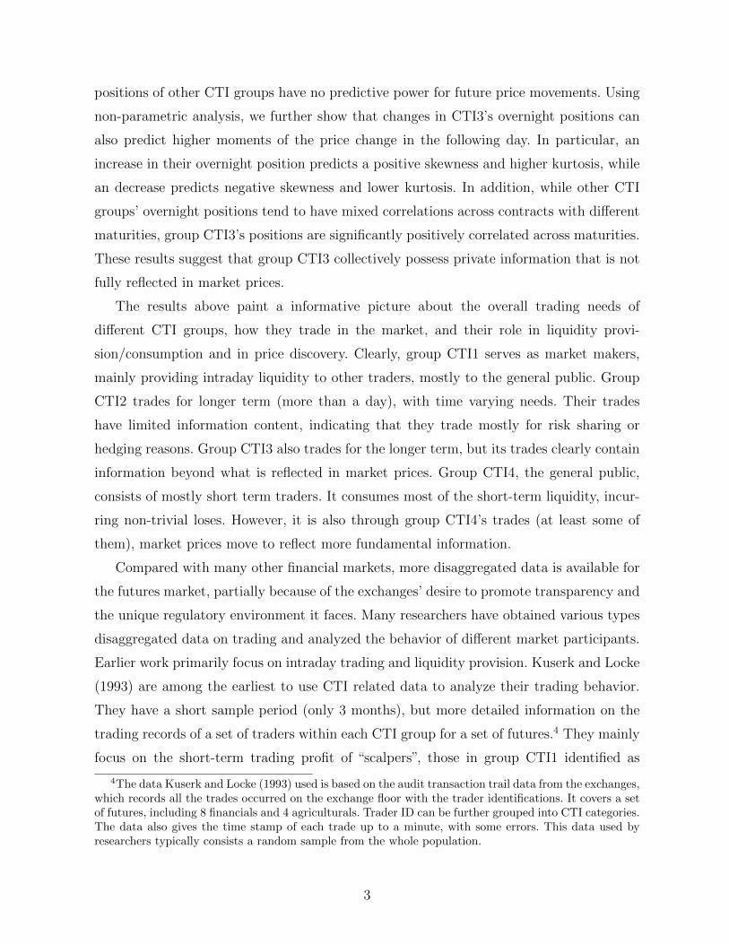
Figure 1 shows the “life-cycle” of contracts with staggering maturities in their open
interests, which are correlated with their liquidity. To avoid potential liquidity issues,
sometimes we only include the most liquid contracts in our analysis. As Figure 1 shows,
the open interest of a contract drops substantially when it enters its maturing month (and
so is its liquidity). Also, for contracts with the longest maturities, their open interests are
also very low. Thus, we define m = 1, 2, 3, 4 as the most liquid contracts.20 As the data
shows, they represent over 91% of the total open interest and 95% of the total volume in
the market.
To simplify our analysis and presentation, sometimes we use the market average for
certain variables instead of looking at each individual contract. Factoring in liquidity con-
19Daigler and Wiley (1999) used the Graman and Klass (1980) volatility measure as well as the differencebetween the high minus low prices to study the influence of CTI’s traded volume on market volatility forthe silver, munis, MMI index, T-notes and T-bonds futures markets, using daily data from June 1986 toJune 1998. The results of their regressions are similar for both measures.
20The time series for the considered variables are formed by rolling the contracts the first day of thedelivery month to contracts with the next nearest delivery month. Changes in prices are calculated alwaysusing prices on the same contract.
10

Jan2001 Apr2001 Jul2001 Oct2001 Jan20020
0.5
1
1.5
2
2.5
3x 10
5
Dates
Ope
n in
tere
st b
y co
ntra
cts
200103 n=346
200105 n=326
200107 n=417
200109 n=369
200112 n=608
200203 n=329 .
200205 n=327 .
200207 n=493 .
200212 n=735 .
200209 n=369 .
Figure 1: Open interest for different maturities. The figure plots the open interest of tradedcontracts during the year of 2001. The maturities of these contracts are March, May, July,September, December of 2001 and March, May, July, September and December of 2002,respectively.
siderations, we only include the four most liquid contracts. In particular, we have
Pt =1
4
4∑m=1
P(m)t (3a)
Xt =1
4
4∑m=1
X(m)t =
1
4
4∑m=1
HML(m)t /P
(m)t . (3b)
From the LDB data, for each contract we can obtain the buy and sell transactions
of each CTI group for each transaction price during the day and the time intervals they
belong. For date t and contact m, let F(m)tk denote the k-th transaction price, where k =
1, . . . , Kt. We then have, for each CTI group i and contract m,
F(m)tk = the k-th transaction price during date t, k = 1, . . . , Kt (4a)
B(m)i,tk = number of contracts bought at transaction price F
(m)tk by CTI group i (4b)
S(m)i,tk = number of contracts sold at transaction price F
(m)tk by CTI group i. (4c)
It is important to recognize that LDB does not provide the precise information on the
time of a transaction. It only gives the time intervals, in half-hour brackets, during which
a trade at a given transaction price occurred.21 Thus, the trade index here does not really
21There may be multiple transactions at a given price in a day, falling into different half-hour time
11

describe the sequencing of trades within a bracket. Since the time interval of our analysis
is over a day, we further ignore the time bracket of a trade.
Following the convention established above, we will add subscript i for CTI group i,
i = 1, 2, 3, 4, and superscript (m) for contract m, m = 0, 1, 2, 3, 4, . . ., to these and other
variables when needed.
From the transactions data, we construct several additional variables on each CTI
group’s trading activity. In particular, we can define the change in CTI group i’s position
in a given contract m in date t by
∆N(m)i,t =
∑k
(B
(m)i,tk − S
(m)i,tk
), i = 1, 2, 3, 4. (5)
If we start from the beginning of trading for a contract, we can further construct the
cumulative position in a contract by a CTI group at the close of each trading day by
N(m)i,t =
t∑s=0
∆N(m)i,s , i = 1, 2, 3, 4. (6)
We also define the sum of changes in positions over all contracts, i.e., m = 1, 2, 3, 4, . . ., as
a measure of change in each CTI group’s net positions:
∆Ni,t =∑m
∆N(m)i,t . (7)
Adding up the changes in a CTI group’s net positions will yield the cumulative net position
of the group at the close of each trading day:
Ni,t =∑m
N(m)i,t =
∑m
t∑s=0
∆N(m)i,s , i = 1, 2, 3, 4. (8)
We can also compute the trading volume of each CTI group from LDB transactions for
each contract, by the number of contracts and dollar amount, respectively, as follows:
V(m)i,t =
∑k
(∣∣B(m)i,tk
∣∣+∣∣S(m)
i,tk
∣∣) , V$(m)i,t =
∑k
(∣∣B(m)i,tk
∣∣+∣∣S(m)
i,tk
∣∣)F (m)tk . (9)
Summing over the four groups gives the trading volume for a given contract:
V(m)t =
1
2
4∑i=1
V(m)i,t , V
$(m)t =
1
2
4∑i=1
V$(m)i,t (10)
intervals. The LDB data does not specify which one of these intervals a particular transaction belongs.
12
where the coefficient 1/2 corrects for double counting.
It is worth noting that even though EOD files also provide data on daily trading volume,
we do not use it for our volume measure. This is because the volume number in EOD files
also contains electronic transactions (outright and spread trades), pit spread trades and
ex-pit transactions (block trades, EFP, EFR, etc.), which are not included in our entire
LDB sample. To be consistent, we use the LDB data to construct a better matched volume
measure. Moreover, in our LDB volume data all trades are competitively determined and
netted trades, for each buy side there is one sell side. The difference between the volume
measure from LDB data and EOD data is relatively small. The two measures are highly
correlated (the correlation coefficient is 0.983). Appendix A.1 provides a more detailed
comparison between these two measures. More importantly, our results do not depend on
the choice between the two measures. Following this procedure and staying as close as
possible to one consistent source of data, we built the HML(m)t data from the LDB files.
The correlation between this series and the one from the OED file is 0.98. Note also that
the prices used in the HML(m)t variable are transaction prices with non-trivial volume
attached—they are not quoted prices.
Summing over all contracts give us a measure of volume for the overall market:
Vt =∑m
V(m)t , V $
t =∑m
V$(m)t . (11)
Using the data of daily open interest from the EOD files, we can also define a measure
of turnover for the whole market by:
τt =VtOIt
, OIt =∑m
OI(m)t . (12)
In a similar way to Fishman and Longstaff (1992), we also compute each CTI group’s
P&L (profit and loss) from its intraday transactions in a given contract m by:
PNL0 (m)i,t = −
∑k
(B
(m)i,tk − S
(m)i,tk
)F
(m)tk + ∆N
(m)i,t P
(m)t (13)
where P(m)t is the settlement price of the m contract for date t. This definition takes into
account the mark to market for futures positions taken during the date. It, however, does
not include the P&L from the mark to market on remaining positions from the previous
13

day, which is N(m)i,t−1(P
(m)t − P (m)
t−1 ). We call this part the interday P&L:22
PNL1 (m)i,t = N
(m)i,t−1
(P
(m)t − P (m)
t−1
)(14)
Thus, the total P&L (for a given CTI group and contract) is given by:
PNL(m)i,t = PNL
0 (m)i,t + PNL
1 (m)i,t . (15)
Summing over all contracts, we obtain the total P&L for each CTI group:
PNLi,t =∑m
PNL(m)i,t . (16)
In addition, we introduce a variable that measures the daily “imbalance” in the trading
of a contract between the buy and and sell side. In particular, on each trading day for
each contract, we first divide the range of transaction prices into three intervals with equal
number of distinctive prices. We then compute the dollar volume for prices in each of
the intervals. Taking the difference between the dollar volume in the top and the bottom
interval reflects the imbalance in trading on the buy and sell side. We sum this imbalance
in dollar volume over the four most liquid contracts, i.e., m = 1, 2, 3, 4, and normalize it
by the total dollar volume to arrive at our measure of market-wide imbalance in trading:
Zt =1
4
4∑m=1
V$(m)t (top price interval)− V $(m)
t (bottom price interval)
V $t
. (17)
2.3 Data Summary
In this section, we present a brief summary of the data. Figure 2 shows the time series of
the average daily settlement price, Pt, and average difference between high and low prices
reached during each trading day, normalized by the settlement price, Xt, over the whole
sample period.
In Panel (a), we plot the daily settlement price averaged over the four liquid contracts
(m = 1, 2, 3, 4). It is interesting to note that the level of corn futures price remained
relatively stable over this period. It peaked in 1996, reaching above $4.5/bushel briefly.23
22Hartzmark (1987) noted that this is the procedure used by the central clearing house to mark eachtrader’s account to the market price at the end of each trading session: multiply the end-of-day positionby the change in the settlement price.
23A USA Midwestern drought on 1995-96, rising foreign demand for US grains (corn, wheat and soybean)particularly from China, and substantial commodity market speculation combined into a markedly drive
14

1995 1996 1997 1998 1999 2000 2001 2002 2003 2004 2005 2006
2
2.5
3
3.5
4
Dates
Pt (d
olla
rs/b
ushe
l)
1995 1996 1997 1998 1999 2000 2001 2002 2003 2004 2005 2006
−0.04
−0.02
0
0.02
0.04
0.06
Dates
Δ ln
Pt
(a) (b)
1995 1996 1997 1998 1999 2000 2001 2002 2003 2004 2005 2006
1
2
3
4
5
6
7
Dates
Xt,
ldb (%
)
1995 1996 1997 1998 1999 2000 2001 2002 2003 2004 2005 2006
−0.04
−0.03
−0.02
−0.01
0
0.01
0.02
0.03
0.04
Dates
Δ X
t, ld
b (%)
(c) (d)
Figure 2: History of settlement price and normalized high minus low prices. This figureshows the time series of the market average (over the four nearest contracts) of settlementprices (Pt) and normalized high minus low prices during a trading date (Xt) over the sampleperiod. Panel (a) plots the average daily settlement price, Panel (b) plots the average ofchanges in the logarithm of daily settlement price, Panel (c) plots the average of high minuslow prices reached during each trading day, normalized by the settlement price, and Panel(d) plots the average of changes in the normalized high minus low prices of each day.
But for most part of the sample, it stayed between $2 to $3 per bushel, despite the relatively
long time span of over 10 years. Panel (b) of Figure 2 plots the daily change in the logarithm
of settlement prices averaged over the four most liquid contracts. Clearly, the distribution
is relatively stable over time, with an indication of seasonality, which is well known for this
market.
In Panel (c) of Figure 2, we plot the average of high minus low prices reached during each
trading day, normalized by the settlement price. Again, its distribution seems reasonably
stable, but exhibits clear seasonality. Panel (d) further plots the daily changes in the
relative high minus low prices, which exhibits fairly stable distributions.
Figure 3 describes the history of overall trading activities in this market. Panel (a) of
Figure 3 plots the time series of the overall market open interest at the end of each trading
up in prices in 1995 and 1996, reaching the highest price on July 2, 1996 with $5.545/bushel, rationeddemand and subsequent crops replenished stocks drove prices down to usual levels
15

day. It stayed relatively stable, ranged between 250,000 to 500,000 contracts, until 2004,
and then started to increase substantially, exceeding 1,200,000 contracts by the end of our
sample period. In Panel (b), we plot the daily trading volume, in the number of contracts.
It exhibits a similar pattern as the open interest, stayed relatively stable in the early part
of the sample but started to increase after 2004. Another interesting feature about daily
trading volume is that its daily variation is quite substantial.
1995 1996 1997 1998 1999 2000 2001 2002 2003 2004 2005 2006
300
400
500
600
700
800
900
1000
1100
1200
Dates
OI t (i
n th
ousa
nd c
ontr
acts
)
1995 1996 1997 1998 1999 2000 2001 2002 2003 2004 2005 2006
20
40
60
80
100
120
140
160
180
200
Dates V
t, ld
b (in
thou
sand
con
trac
ts)
(a) (b)
Figure 3: Open interest and trading volume. Panel (a) of the figure plots the total openinterest in all traded contracts at the end of each trading day (OIt) and Panel (b) plots thetotal trading volume, in the number of contracts, Vt.
A commonly used measure of trading activity is turnover. Figure 4 shows the daily
time series of the turnover measure defined in Equation (12), which is volume normalized
by open interest. Despite the increase in open interest and trading volume during the last
three years of the sample, the turnover did not increase, as shown in Panel (a). In fact,
it seemed to have decreased a bit, reflecting the fact that volume may not have increased
proportionally with open interest. In Panel (b), we plot the daily changes in turnover,
which seems to have a more stable distribution over the sample period, except toward the
last two years, for reasons mentioned earlier.
In Table 1, we provide some summary statistics for several of the variables defined
above. The p-value is provided in the parenthesis as in all tables in this paper. Clearly, the
daily change in the average log settlement price has a sample mean of zero and a daily
volatility of 1.3%. It also exhibits a mild positive skewness and a substantial kurtosis,
which reflects the fat-tails in its distribution. In addition, the change in log price has a
weak but statistically significant serial correlation at one-day lag and a seasonal five-day
lags, but the correlation dies off with more lags. This weak serial correlation will be taken
into account in our future analysis of the price formation process.
16

1995 1996 1997 1998 1999 2000 2001 2002 2003 2004 2005 2006
5
10
15
20
25
30
35
40
Dates
τ t, ld
b (%)
1995 1996 1997 1998 1999 2000 2001 2002 2003 2004 2005 2006
−20
−15
−10
−5
0
5
10
15
20
25
30
Dates
Δ τ t,
ldb (%
)
(a) (b)
Figure 4: Daily turnover and changes in turnover. Panel (a) plots the daily turnover τt.Panel (b) plots the daily changes in turnover ∆τt.
Table 1: Descriptive statistics for the market variables.
mean std skew kurt ρ1 ρ2 ρ5 ρ10
Pt 2.529 0.425 1.499 5.091
OIt(×1, 000) 460.559 162.867 1.917 7.567
Xt(%) 1.526 0.793 1.551 6.636 0.373 0.381 0.326 0.292(0.000) (0.000) (0.000) (0.000)
Vt(×1, 000) 51.112 23.553 1.575 7.320 0.510 0.443 0.350 0.302(0.000) (0.000) (0.000) (0.000)
τt(%) 11.576 5.124 1.506 6.532 0.471 0.396 0.292 0.248(0.000) (0.000) (0.000) (0.000)
Zt -0.007 0.054 0.059 3.601 0.086 0.060 0.002 0.011(0.000) (0.001) (0.903) (0.556)
∆ lnPt -0.000 0.013 0.185 4.800 0.053 0.019 -0.051 0.005(0.004) (0.305) (0.006) (0.808)
∆Xt -0.000 0.009 0.243 5.716 -0.506 0.029 0.014 -0.007(0.000) (0.121) (0.464) (0.726)
∆τt(%) 0.000 5.265 0.519 6.663 -0.428 -0.015 0.018 0.003(0.000) (0.421) (0.339) (0.878)
This table shows the descriptive statistics for daily average of the market variables. ρi denotes theautocorrelation coefficient for lag i. The sample period is 1995-2006. The p-values are provided insidethe parenthesis.
The normalized difference between the high and low prices during a day, Xt =
14
∑4m=1HML
(m)t /P
(m)t , roughly reflects the daily price variation (with a sample mean
of 1.5%). It exhibits similar positive skewness and kurtosis as the change in log prices. It
also exhibits a strong serial correlation, which persists even after many lags. For example,
even at 10-day lags, the serial correlation of Xt remains at 0.292 and highly significant.
17

This is consistent with the general property of the financial market that price volatility is
highly persistent over time. However, when we look at the changes in Xt, i.e., ∆Xt, the
serial correlation is significantly negative at one lag, but becomes insignificant afterwards.
The average level of daily turnover in the sample is 11.576%, which means that daily
trading volume is on average over 11% of the end-of-day open interest. This clearly suggests
that in this market there is high level of intraday trading. As is typically the case for
measures of trading activities, τt exhibits positive skewness and kurtosis. Moreover, our
turnover measure has persistent serial correlation. However, when we look at changes in
the turnover, it has a strong serial correlation at only one lag, which is negative, reflecting
strong mean reversion tendency in the level of turnover. The serial correlation becomes
insignificant even at the 2-day lag.
The measure of trading imbalance, Zt, has a small and negative sample mean. It exhibits
no skewness but a non-trivial kurtosis. It is positively serially correlated but only at one-
and two-day lags. The correlation, even though statistically significant, is quite small.
Table 2: Correlations among the changes in the market variables.
∆ lnPt ∆τt ∆Xt Zt
∆ lnPt 1.000 0.006 0.046 0.425(0.000) (0.742) (0.016) (0.000)
∆τt 1.000 0.667 0.004(0.000) (0.000) (0.828)
∆Xt 1.000 0.043(0.000) (0.023)
Zt 1.000(0.000)
This tables shows the correlations among the changes in the market variables. The sampleperiod is 1995-2006. The p-values are provided inside the parenthesis.
In Table 2, we report the correlation between the main market variables we will use
in future analysis. It is not surprising that there is strong correlation (0.667) between
turnover τt and normalized high minus low prices. It is well known that turnover and price
volatility are related in the futures market (as well as in other financial markets).24 We also
24Bessembinder and Seguin (1993) examined eight futures, including two currencies (Deutsche markand Japanese yen), two metals (gold and silver), two agricultural products (cotton and wheat) and twofinancials (T-bonds and T-bills), using daily data for the period of May 1982 through March 1990, and
18
see a significant correlation between changes in log settlement price and trading imbalance,
which is 0.425.
As Table 1 shows, the market variables such as turnover and normalized high minus
low prices exhibit significant persistence. This persistence still exists even for first order
differences. In our future analysis, we will use first differences to describe the dynamics of
these market variables. Moreover, we use an MA(2) model to characterize the dynamics of
the first differences of these market variables, and to decompose them into their expected
and unexpect parts.25 See Appendix A.3 for the details of these decompositions.
The discussion above focuses mostly on market-wide variables. In particular, we ag-
gregate across contracts with different maturities and over different CTI groups. In the
following sections, we will examine in detail the behavior of different CTI groups and its
connection with prices. Here, we provide some information on the distribution of trading
over contracts with different maturities.
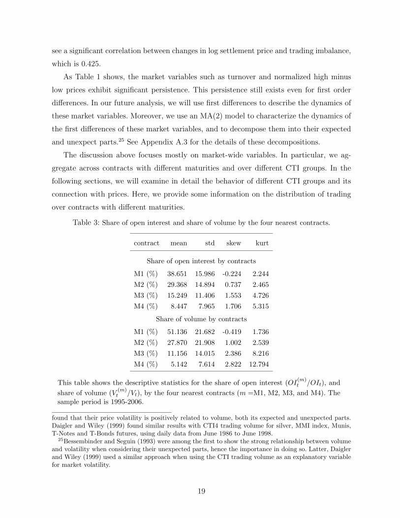
Table 3: Share of open interest and share of volume by the four nearest contracts.
contract mean std skew kurt
Share of open interest by contracts
M1 (%) 38.651 15.986 -0.224 2.244
M2 (%) 29.368 14.894 0.737 2.465
M3 (%) 15.249 11.406 1.553 4.726
M4 (%) 8.447 7.965 1.706 5.315
Share of volume by contracts
M1 (%) 51.136 21.682 -0.419 1.736
M2 (%) 27.870 21.908 1.002 2.539
M3 (%) 11.156 14.015 2.386 8.216
M4 (%) 5.142 7.614 2.822 12.794
This table shows the descriptive statistics for the share of open interest (OI(m)t /OIt), and
share of volume (V(m)t /Vt), by the four nearest contracts (m =M1, M2, M3, and M4). The
sample period is 1995-2006.
found that their price volatility is positively related to volume, both its expected and unexpected parts.Daigler and Wiley (1999) found similar results with CTI4 trading volume for silver, MMI index, Munis,T-Notes and T-Bonds futures, using daily data from June 1986 to June 1998.
25Bessembinder and Seguin (1993) were among the first to show the strong relationship between volumeand volatility when considering their unexpected parts, hence the importance in doing so. Latter, Daiglerand Wiley (1999) used a similar approach when using the CTI trading volume as an explanatory variablefor market volatility.
19

Table 3 reports some summary statistics for the share of total open interest and trading
volume of the four most liquid contracts, m = 1, 2, 3, 4, denoted by M1, M2, M3, and
M4, respectively in the table. Not surprisingly, the most liquid contract, which is also
the contact with the nearest maturity (excluding the contract soon to mature), has over
38% of the total open interest. The next maturity has about 29% and it tapers off quite
quickly. The fourth contract (m = 4) has about 8%. The distribution of trading volume
across contracts with different maturities exhibits the same pattern. The nearest contract
contributes 51% to the total trading volume. The next contract contributes around 27%.
The volume share drops to around 11% and 5%, respectively, for the next maturities. Thus,
as it was already mentioned, the first four maturities represent over 91% of the total open
interest and over 95% of the total trading volume in the corn market futures. The above
distribution of trade among maturities is the reason why in our analysis of price discovery
process in this market, we will primarily focus on either the nearest contract or the four
nearest contracts.
3 Trading and Profits of CTI Groups
3.1 Trading Behavior
We now examine the trading behavior of the four CTI groups. From the LDB, we can
construct the trades of each CTI group in each contract. We can then compute the daily
trading volume and the net change in positions. The former gives us picture about the
relative share of each group in trading while the latter describes its net overnight position
taking.
In Figure 5, we plot the relative share of the total trading volume (including all con-
tracts) of each CTI group. It is obvious that group CTI1 has the largest share of the total
volume. Over the sample period, it typically has more than 50% of the volume. Group
CTI4 is the next most active in trading, contributing to between 30% to 40% of the total
volume. Both groups CTI2 and CTI3 have typically less than 10% of the total volume
each. Group CTI2 has less than 5% share of the volume until 2004 when the volume share
jumped close to 10%.26
26For the five futures and the two-year period (June 1986 through June 1988) they cover, Daigler andWiley (1999) report (Table I) the following volume breakdowns by CTI groups (means calculated for thisfootnote): 50% for CTI1, 16% for CTI2, 7% for CTI3 and 27% for CTI4. Fishman and Longstaff (1992)report that the CTI1 represent nearly 60% of the total volume for the 15 random days on the last quarter
20

1995 1996 1997 1998 1999 2000 2001 2002 2003 2004 2005 2006
10
20
30
40
50
60
Dates
V1,
t/Vt (%
)
1995 1996 1997 1998 1999 2000 2001 2002 2003 2004 2005 2006
10
20
30
40
50
60
Dates
V2,
t/Vt (%
)
(a) (b)
1995 1996 1997 1998 1999 2000 2001 2002 2003 2004 2005 2006
10
20
30
40
50
60
Dates
V3,
t/Vt (%
)
1995 1996 1997 1998 1999 2000 2001 2002 2003 2004 2005 2006
10
20
30
40
50
60
Dates
V4,
t/Vt (%
)
(c) (d)
Figure 5: Share of trading volume by CTI groups. This figure shows the total tradingvolume of each CTI group (Vi,t) normalized by the market volume (Vt) in percentage terms,over the sample period. Panel (a) is for CTI1, Panel (b) CTI2, Panel (c) CTI3 and Panel(d) CTI4.
It is worth noting that over the same period, the trading of group CTI2 has increased
and that of CTI4 has decreased accordingly. This change is in part due to some of the
reclassification of trades between the groups during 2004.27
Among the trades during a day by a CTI group, some are offsetting with each other.
This part of the trading can be labeled as “intraday” trading (some authors name them as
“round trip trading”). The change in the net position from the previous day, i.e., ∆N(m)i,t ,
can then be labeled as “interday” trading. We refer to its absolute value as the interday
trading volume. The breakdown of a CTI group’s into these two parts is indicative of its
trading behavior and potential trading motive. Figure 6 plots the interday trading volume
by each CTI group, normalized by the group’s own daily volume.
The difference across different CTI groups is stark. For group CTI1, most of its trading
of 1998 in the soybean market. Manaster and Mann (1996) look at all the futures traded on CME duringthe first half of 1992 and find that CTI1 represents 47% of the total volume, CTI2 7%, CTI3 6% and CTI440%.
27See the Appendix A.2 for the re-classification, or “Harmonization”, on the CTI codes on CME andCBOT.
21

1995 1996 1997 1998 1999 2000 2001 2002 2003 2004 2005 20060
10
20
30
40
50
60
70
80
90
100
Dates
abs
(Δ N
1,t)/V
1,t (%
)
1995 1996 1997 1998 1999 2000 2001 2002 2003 2004 2005 20060
10
20
30
40
50
60
70
80
90
100
Dates
abs
(Δ N
2,t)/V
2,t (%
)
(a) (b)
1995 1996 1997 1998 1999 2000 2001 2002 2003 2004 2005 20060
10
20
30
40
50
60
70
80
90
100
Dates
abs
(Δ N
3,t)/V
3,t (%
)
1995 1996 1997 1998 1999 2000 2001 2002 2003 2004 2005 20060
10
20
30
40
50
60
70
80
90
100
Dates
abs
(Δ N
4,t)/V
4,t (%
)
(c) (d)
Figure 6: Interday trading volume by each CTI group relative to its total volume. This figureshows the interday volume of each CTI group (|∆Ni,t|) normalized by its total volume (Vi,t),in percentage terms. Panels (a), (b), (c) and (d) are for groups CTI1, CTI2, CTI3 and CTI4,respectively.
is intraday. Its interday volume is only a tiny fraction of its total volume.28 The same is true
for group CTI4, although the share of interday trading is slightly higher. For groups CTI2
and CTI3, however, interday trading constitutes a large fraction of their total volume. For
group CTI2, often more than 50% of its trading is interday and sometimes it reaches 80%
or higher. For group CTI3, the share of interday trading typically ranges between 20% to
50%.29
The two figures above give the following picture: Groups CTI1 and CTI4 produce
28When analyzing the inventory of the market makers (CTI1) in all the futures traded on CME usingtransactions data for the first half of 1992, Manaster and Mann (1996) point to three possible sources forthe“nonzero daily inventory changes.”One may be due to CTI3 trades and the other two are potential dataerrors and the overnight unwinding of positions in SIMEX (Singapore International Monetary Exchange).
29Studying the futures energy markets in the NYMEX and using daily open interest positions of indi-vidual traders, Dewally et al. (2013) find that the group of “market makers/floor traders” (correspondingto CTI1 or CTI1 plus CTI3 in our grouping) is the one with the highest interday turnover (daily change inpositions of the group over its own open interest position). Our findings are consistent but cover to othermarket participants.
22

most of the trading volume. But most of their trading is intraday. Groups CTI2 and
CTI3, however, do not contribute much to the intraday volume. Nonetheless, their trading
is mostly interday, which constitutes most of the interday volume. As we will see later,
this distinction in different CTI groups’ trading behavior is closely related to their trading
motive, the role they play in liquidity provision and consumption and in the price formation
process.
Next, we examine in more detail different CTI groups’ interday trading, i.e., overnight
position taking. We first note that theoretically all groups’ net interday trading has to sum
up to zero. This implies that the net daily changes in the CTI groups’ interday positions
are not dependent. In Table 4, we report the correlations between net changes in the total
positions of each CTI groups. It is interesting to note that the daily position changes
of group CTI4 is significantly negatively correlated with that of groups CIT1, CTI2 and
CTI3. The other correlations are all relatively small. This suggests that to a large extent,
for interday trades, group CTI4 is usually on one side and the other three groups are on
the other side.
Table 4: Correlations among changes in overnight positions by different CTI groups.
CTI1 CTI2 CTI3 CTI4
CTI1 1.000 -0.026 0.031 -0.526(0.000) (0.174) (0.104) (0.000)
CTI2 1.000 -0.034 -0.491(0.000) (0.069) (0.000)
CTI3 1.000 -0.683(0.000) (0.000)
CTI4 1.000(0.000)
This table shows the correlations among changes in overnight positions for the CTI groups(∆Ni,t, i = 1, 2, 3, 4). The sample period is 1995-2006. The p-values are provided inside theparenthesis.
Several previous studies, such as Manaster and Mann (1996), Daigler and Wiley (1999),
and Ferguson and Mann (1999), find the same result that trading between locals (CTI1)
and customers (CTI4) accounts for a large part of the total volume.30 Based on a longer
30Based on the transaction data for all futures trades on the CME during six month of 1992, Manasterand Mann (1999) conclude the following breakdown in terms of share of total volume from trading between:
23

sample, we reconfirm this result and also extend the analysis to provide a more complete
picture in the distribution of volume across different CTI groups for both intraday trading
and interday trading. As we will show later, these trading are driven by different trading
needs of these groups and impact the market in different dimensions.
In the discussions above, we only consider the total overnight position of each CTI
group in the four most liquid contracts. As one might expect, for various reasons such as
hedging or market making, each group (or investor) may hold offsetting positions across
contracts. In Table 5, we report the correlations between the changes of each CTI group’s
overnight positions in contracts with different maturities. Indeed, for groups CTI1, CTI2
and CTI4, changes in interday positions in different contracts often exhibit a mixture
of positive and negative signs. For example, changes in their interday positions in the
nearest contract are often negatively correlated with changes in interday positions in other
contracts (with the exception of of CTI2 and contract 4). However, it is interesting to note
that for group CTI3 all correlations are positive, implying that for this group changes in
positions behave in the same way for all maturities. Contrary to other CTI groups, which
seem to hedge across different maturities, CTI3 group “hedges or bets” the market as a
whole (i.e., taking “directional trade” on the whole market). As we will see in Section 5,
this behavior of group CTI3 is no accident.
Table 6 presents the descriptive statistics for the changes in positions of each CTI group
in all contracts. As in all tables in this paper, the t statistics, corrected for heteroscedasticity
and autocorrelation using the Newey-West procedure, are provided in square-parenthesis
and numbers in bold face indicate significance at the 5% level. Summing the average
position changes across groups the total is zero, meaning we are not losing any trades
across groups. Yet, different groups on average hold different positions by the end of each
day. In particular, group CTI2 and CTI3 finish each day with long positions on average,
while group CTI1 and CTI4 finish each day with short positions. It is worth noting that
changes in the overnight positions of CTI3 group changes are the most substantial and
exhibit significant term persistence. Changes in the overnight positions of CTI4 exhibit
locals (CTI1) and customers (CTI4) 41%, customers and other customers 11%, commercials (CTI2) andcustomers 9%, floor hedgers (CTI3) and customers 4%, locals and locals 9%, locals and commercials 15%,and locals and floor hedgers 6%. For the five futures markets during the two years (June 1986 throughJune 1998) considered by Daigler and Wiley (1999), they find that groups CTI1 and CTI4 have the highestcross correlation in trading volume among the four CTI groups. Ferguson and Mann (1999) also find thatcustomer trading (CTI4) against any other CTI groups takes between 51% to 75% of the total volume,with the minimum (50%) in Eurodollar and the maximum (75%) in lumber futures.
24

Table 5: Correlations between changes in interday contract positions for each CTI group.
∆N1,t ∆N2,t
M1 M2 M3 M4 M1 M2 M3 M4
M1 1.000 -0.545 -0.418 -0.217 1.000 -0.085 -0.143 0.076(0.000) (0.000) (0.000) (0.000) (0.000) (0.000) (0.000) (0.000)
M2 1.000 -0.129 -0.168 1.000 0.081 -0.062(0.000) (0.000) (0.000) (0.000) (0.000) (0.001)
M3 1.000 0.008 1.000 -0.007(0.000) (0.657) (0.000) (0.714)
M4 1.000 1.000(0.000) (0.000)
∆N3,t ∆N4,t
M1 M2 M3 M4 M1 M2 M3 M4
M1 1.000 0.100 0.079 0.058 1.000 -0.357 -0.277 -0.159(0.000) (0.000) (0.000) (0.002) (0.000) (0.000) (0.000) (0.000)
M2 1.000 0.117 0.060 1.000 -0.109 -0.112(0.000) (0.000) (0.001) (0.000) (0.000) (0.000)
M3 1.000 0.109 1.000 -0.007(0.000) (0.000) (0.000) (0.720)
M4 1.000 1.000(0.000) (0.000)
This table shows the correlations between changes in interday positions (∆Ni,t) in different contracts(M1, M2, M3, and M4) for each CTI group (i = 1, 2, 3, 4). The sample period is 1995-2006. Thep-values are provided inside the parenthesis.
similar behavior but with smaller magnitudes.
3.2 Profit and Loss (P&L)
We now consider the profitability of different CTI groups in their trading. As discussed
in Section 2.2, we decompose the profit of each CTI group into two components: intraday
profits defined in Equation (13), which arises from their intraday trading, and interday
profits defined in Equation (14), which arises from their overnight positions.
In Figure 7, we plot the daily intraday P&L (profit and loss) for each CTI group,
normalized by the group’s own daily volume, and the cumulative normalized intraday P&L
over the sample period. Since groups CTI1 and CTI4 do most of the intraday trading, as
shown by panels (a) and (d) of Figure 5, their bear a substantial amount of intraday
P&L. Furthermore, from panels (b) and (h) of Figure 7, we clearly see that group CTI1
consistently makes money on intraday trading while group CTI4 consistently loses money.
25

Table 6: Descriptive statistics for changes in positions of each CTI group.
mean median std skew kurt ρ1 ρ2 ρ5 ρ10
∆N1,t -126.998 -106.000 947.973 -0.708 22.777 -0.105 -0.003 0.011 0.006[ -7.021] [ -8.800] (0.000) (0.866) (0.555) (0.735)
∆N2,t 56.821 7.000 964.583 0.610 44.136 0.080 0.118 0.025 0.027[ 2.462] [ 3.086] (0.000) (0.000) (0.181) (0.146)
∆N3,t 276.417 257.000 1251.306 -0.088 6.143 0.179 0.167 0.093 0.038[ 7.866] [ 9.858] (0.000) (0.000) (0.000) (0.045)
∆N4,t -206.239 -249.000 1827.064 0.375 11.608 0.081 0.107 0.043 0.009[ -4.635] [ -5.809] (0.000) (0.000) (0.021) (0.643)
This table shows the descriptive statistics for the changes in positions (∆Ni,t, i = 1, 2, 3, 4) of eachCTI group. ρi denotes the autocorrelation for lag i. The sample period is 1995-2006. The p-valuesare provided inside the parenthesis, and the t- statistics are provided in square brackets. Boldfacemeans significative at the 5% level.
This demonstrates that group CTI1 as market makers are compensated from their liquidity
provision. This result is consistent with Manaster and Mann (1996), who observe that
market makers are not only “passive order fillers”, they also manage their inventory as
“active profit-seeking individuals.” They make profits from both execution and timing,
taking advantage of the information they have over the next price movements.
On the other hand, group CTI4 is paying for the liquidity in their intraday trading.
Group CTI2 does only a small amount of intraday trading, as Figure 5(b) shows. Thus, it
incurs little intraday P&L, as shown in Figure 7(d). Group CTI3, on the other hand, does
some intraday trading, for which it pays a non-trivial amount. As Figure 7(f) shows, over
time, group CTI3 consistently loses money in their intraday trading.
Table 7 reports the basic summary statistics for the normalized intraday P&L of each
CTI group. Clearly, group CTI1 has a positive and significant average daily P&L from
intraday trading, while groups CTI3 and CTI4 have significantly negative average P&L
from intraday trading. Since the P&L numbers are normalized by each group’s own daily
volume (by the number of contracts), multiplied by 100, they give the average profit and
loss per contract traded, in cents. Thus, for group CTI1, it earns an average profit of 0.034
cents per contract traded, while for groups CTI3 and CTI4, they on average incur a loss
of 0.028 and 0.041 cents, respectively. Group CTI2, however, incurs no profit or loss for its
intraday trading. Another striking feature of the daily P&L from intraday trading is that
it is highly persistent over time. For example, for group CTI1, its daily intraday P&L has
a serial correlation of 0.150 even after 10 days.
26

1995 1996 1997 1998 1999 2000 2001 2002 2003 2004 2005 2006−5
−4
−3
−2
−1
0
1
2
3
4
5
Dates
(PL 1,
t0
/V1,
t)*100
1995 1996 1997 1998 1999 2000 2001 2002 2003 2004 2005 2006
−100
−80
−60
−40
−20
0
20
40
60
80
Dates
Σs=
0t
(PL 1,
t0
/V1,
t)*10
0
(a) (b)
1995 1996 1997 1998 1999 2000 2001 2002 2003 2004 2005 2006−5
−4
−3
−2
−1
0
1
2
3
4
5
Dates
(PL 2,
t0
/V2,
t)*100
1995 1996 1997 1998 1999 2000 2001 2002 2003 2004 2005 2006
−100
−80
−60
−40
−20
0
20
40
60
80
Dates
Σs=
0t
(PL 2,
t0
/V2,
t*100
(c) (d)
1995 1996 1997 1998 1999 2000 2001 2002 2003 2004 2005 2006−5
−4
−3
−2
−1
0
1
2
3
4
5
Dates
(PL 3,
t0
/V3,
t)*100
1995 1996 1997 1998 1999 2000 2001 2002 2003 2004 2005 2006
−100
−80
−60
−40
−20
0
20
40
60
80
Dates
Σs=
0t
(PL 3,
t0
/V3,
t)*10
0
(e) (f)
1995 1996 1997 1998 1999 2000 2001 2002 2003 2004 2005 2006−5
−4
−3
−2
−1
0
1
2
3
4
5
Dates
(PL 4,
t0
/V4,
t)*100
1995 1996 1997 1998 1999 2000 2001 2002 2003 2004 2005 2006
−100
−80
−60
−40
−20
0
20
40
60
80
Dates
Σs=
0t
(PL 4,
t0
/V4,
t)*10
0
(g) (h)
Figure 7: Intraday P&L of each CTI group over its daily volume (PNL0i,t/Vi,t) and their
corresponding cumulative (∑t
s=0 PNL0i,s/Vi,s), multiplied by 100. The left panels (a), (c),
(e) and (g) are daily intraday P&L for groups CTI1, CTI2, CTI3, and CTI4, respectively,and the right panels are the corresponding cumulative intraday P&L.
27
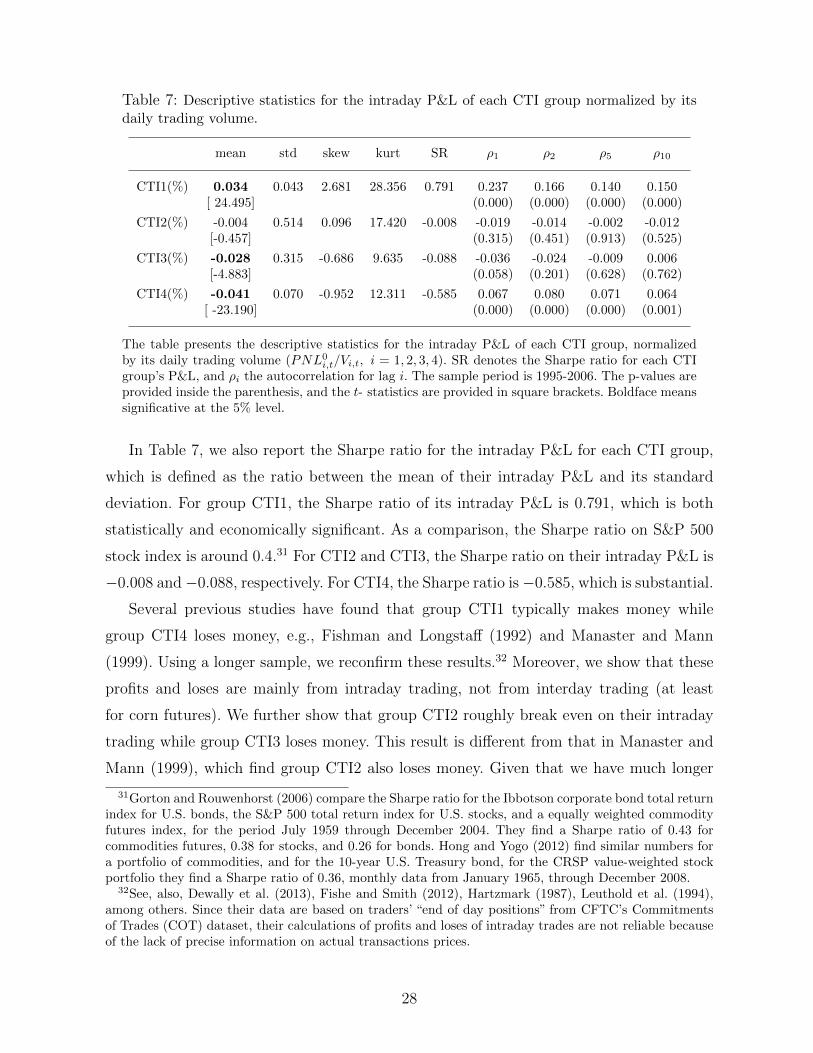
Table 7: Descriptive statistics for the intraday P&L of each CTI group normalized by itsdaily trading volume.
mean std skew kurt SR ρ1 ρ2 ρ5 ρ10
CTI1(%) 0.034 0.043 2.681 28.356 0.791 0.237 0.166 0.140 0.150[ 24.495] (0.000) (0.000) (0.000) (0.000)
CTI2(%) -0.004 0.514 0.096 17.420 -0.008 -0.019 -0.014 -0.002 -0.012[-0.457] (0.315) (0.451) (0.913) (0.525)
CTI3(%) -0.028 0.315 -0.686 9.635 -0.088 -0.036 -0.024 -0.009 0.006[-4.883] (0.058) (0.201) (0.628) (0.762)
CTI4(%) -0.041 0.070 -0.952 12.311 -0.585 0.067 0.080 0.071 0.064[ -23.190] (0.000) (0.000) (0.000) (0.001)
The table presents the descriptive statistics for the intraday P&L of each CTI group, normalizedby its daily trading volume (PNL0
i,t/Vi,t, i = 1, 2, 3, 4). SR denotes the Sharpe ratio for each CTIgroup’s P&L, and ρi the autocorrelation for lag i. The sample period is 1995-2006. The p-values areprovided inside the parenthesis, and the t- statistics are provided in square brackets. Boldface meanssignificative at the 5% level.
In Table 7, we also report the Sharpe ratio for the intraday P&L for each CTI group,
which is defined as the ratio between the mean of their intraday P&L and its standard
deviation. For group CTI1, the Sharpe ratio of its intraday P&L is 0.791, which is both
statistically and economically significant. As a comparison, the Sharpe ratio on S&P 500
stock index is around 0.4.31 For CTI2 and CTI3, the Sharpe ratio on their intraday P&L is
−0.008 and−0.088, respectively. For CTI4, the Sharpe ratio is−0.585, which is substantial.
Several previous studies have found that group CTI1 typically makes money while
group CTI4 loses money, e.g., Fishman and Longstaff (1992) and Manaster and Mann
(1999). Using a longer sample, we reconfirm these results.32 Moreover, we show that these
profits and loses are mainly from intraday trading, not from interday trading (at least
for corn futures). We further show that group CTI2 roughly break even on their intraday
trading while group CTI3 loses money. This result is different from that in Manaster and
Mann (1999), which find group CTI2 also loses money. Given that we have much longer
31Gorton and Rouwenhorst (2006) compare the Sharpe ratio for the Ibbotson corporate bond total returnindex for U.S. bonds, the S&P 500 total return index for U.S. stocks, and a equally weighted commodityfutures index, for the period July 1959 through December 2004. They find a Sharpe ratio of 0.43 forcommodities futures, 0.38 for stocks, and 0.26 for bonds. Hong and Yogo (2012) find similar numbers fora portfolio of commodities, and for the 10-year U.S. Treasury bond, for the CRSP value-weighted stockportfolio they find a Sharpe ratio of 0.36, monthly data from January 1965, through December 2008.
32See, also, Dewally et al. (2013), Fishe and Smith (2012), Hartzmark (1987), Leuthold et al. (1994),among others. Since their data are based on traders’ “end of day positions” from CFTC’s Commitmentsof Trades (COT) dataset, their calculations of profits and loses of intraday trades are not reliable becauseof the lack of precise information on actual transactions prices.
28

sample, while they only have 6 months, our results should be more robust.
Next, we examine the P&L from different CTI groups’ interday trading, i.e., overnight
position taking. In Table 8, we report the basic summary statistics for their interday P&L.
Clearly, group CTI2 on average earns positive profits on its interday trades while group
CIT3 bears a loss on its interday trading. The other two groups, CTI1 and CTI4, have
no significant profit or loss. The other interesting observation is that unlike the P&L from
intraday trading, which exhibits persistence after many lags, P&L from interday trading
exhibits some persistence only over the first a few lags.33
Table 8: Descriptive statistics for the interday P&L of each CTI group, normalized by itsdaily trading volume.
mean std skew kurt SR ρ1 ρ2 ρ5 ρ10
CTI1(%) 0.045 2.358 -0.259 5.460 0.019 0.015 -0.085 -0.025 0.021[1.100] (0.434) (0.000) (0.195) (0.265)
CTI2(%) 0.609 13.491 -0.213 8.254 0.045 0.025 -0.062 -0.018 0.007[ 2.422] (0.182) (0.001) (0.341) (0.696)
CTI3(%) -0.765 19.590 0.002 4.042 -0.039 -0.001 -0.046 -0.027 -0.001[ -2.267] (0.960) (0.016) (0.157) (0.974)
CTI4(%) -0.003 2.715 -0.008 6.866 -0.001 0.038 -0.032 -0.080 0.001[-0.072] (0.042) (0.092) (0.000) (0.946)
This table shows the descriptive statistics for the interday P&L of each CTI group, normalized byits daily trading volume (PNL1
i,t/Vi,t, i = 1, 2, 3, 4). SR denotes the Sharpe ratio for each CTIgroup’s P&L, and ρi the autocorrelation for lag i. The sample period is 1995-2006. The p-valuesare provided inside the parenthesis, and the t- statistics are provided in square brackets. Bold facemeans significative at the 5% level.
Dewally et al. (2013) find that the market makers as a group have significant trad-
ing loses on their overnight positions. Fishe and Smith (2012) find that market makers
are “over-represented” among traders who have positive performance from their overnight
positions.
Our results on the performance of different CTI groups’ overnight positions are less
informative, in part because of the slippage from missing spread trades and ex-pit trades.
3.3 Intraday P&L and Market Variables
In this section, we study how the intraday profits for each CTI group (PNL0i,t) is related
to the market variables, including turnover and normalized high minus low prices. Given
33Remember that our LDB data misses about 30% of the EOD trading volume from non-pit transactions,off hours trades, and potential recording errors.
29

the persistence in P&L, we consider changes in P&L, which still exhibits non-trivial au-
tocorrelation within two lags. We thus decompose the changes in P&L into a predictable
part using an MA(2) model and a residual as follows:
∆PNL0i,t = ∆PNL0
i,t + u0i,∆PNL,t (18)
where ∆PNL0i,t is the forecast of ∆PNL0
i,t from the estimated MA(2) model34. We then
consider how u0i,∆PNL,t can be explained by changes in τt and Xt, i.e., ∆τt and ∆Xt, as
well as the measure imbalance Zt. As control variables, we also include lagged changes
in log settlement prices. All the market variables are averaged over the four most liquid
contracts.
Following Bessembinder and Seguin (1993), we run the regression by decomposing the
highly persistent explanatory variables (changes in volume and volatility) by its forecasted
value based on the MA(2) model and the residual, if the variable shows up significant (see
the appendix for more details). Formally, the relationship we estimate is given as follows:
u0i,∆PNL,t = a + b1∆τ t + b′1u∆τ,t + b2∆X t + b′2u∆X,t + b3Zt
+ lagged changes in log settlement prices as controls. (19)
Since only groups CTI1 and CTI4 incur significant intraday P&L, we report the re-
gression results only for them. Table 9 gives the results for groups CTI1 and CTI4.
From the left panel of Table 9, we see that lagged changes in log prices show certain
statistical significance in explaining changes in intraday P&L for group CTI1. However,
the power is quite weak, with a R-square of less than 1.5%. Trade imbalance measure Zt
has no explanatory power. Both innovations in turnover and price volatility, as measure by
normalized high minus low prices, have significant power in explaining changes in group
CTI1’s intraday P&L. The former yields a R-square of around 15% alone while the latter
gives a R-square of 13% by itself. Together, they explains over 17% of the daily changes
in CTI1 group’s intraday P&L. These results are not surprising. As market makers, one
would expect CTI1 group to make more profits when volume or volatility rises (they
demand higher spread when volatility is high).35
34Given the standard nature of this procedure, we omit the details here, which are given in AppendixA.3.
35Dewally et al. (2013) find a positive relationship between interday profits for the group of speculators,which includes market makers and floor traders, and its trading volume. Chang (1985) analyzes monthlydata on net positions of large hedging, speculative and non-reporting traders and concludes that the
30

Tab
le9:
Reg
ress
ions
ofin
trad
ayP
&L
ofgr
oup
sC
TI1
and
CT
I4on
mar
ket
vari
able
s.
CT
I1C
TI4
c0.
000
0.000
0.00
00.
000
0.00
0-0
.000
-0.0
00-0
.000
-0.0
00-0
.000
[0.2
87]
[0.2
08]
[0.2
42]
[0.3
71]
[0.2
10]
[-0.
198]
[-0.
133]
[-0.
161]
[-0.
288]
[-0.
135]
∆τt
-0.0
02
0.00
3[-
0.371
][0
.485
]ut,
∆τ
0.059
0.042
-0.051
-0.043
[8.3
59]
[4.
993]
[-6
.237
][
-4.5
33]
∆Xt
-0.0
110.
008
[-0.
367]
[0.2
24]
ut,
∆X
t0.349
0.163
-0.273
-0.0
85[
8.35
6][
3.10
9][
-5.3
40]
[-1.
411]
Zt
0.00
2-0
.002
[0.5
62]
[-0.
620]
∆lnPt−
10.041
0.0
22
0.029
0.041
0.02
2-0
.020
-0.0
03-0
.011
-0.0
19-0
.004
[3.0
88]
[1.9
22]
[2.2
82]
[3.0
12]
[1.9
35]
[-1.
030]
[-0.
181]
[-0.
555]
[-0.
979]
[-0.
196]
∆lnPt−
20.039
0.033
0.033
0.039
0.032
-0.036
-0.0
30-0
.032
-0.036
-0.0
31[
3.118
][2
.832]
[2.8
12]
[3.0
65]
[2.8
54]
[-2.
016]
[-1.
691]
[-1.
757]
[-1
.989
][-
1.74
3]∆
lnPt−
30.024
0.0
10
0.01
50.024
0.01
0-0.034
-0.0
21-0
.027
-0.034
-0.0
22[
2.074
][0
.951]
[1.4
17]
[2.0
70]
[0.9
77]
[-2.
364]
[-1.
541]
[-1.
910]
[-2.
361]
[-1.
569]
R2
1.3
62
15.
852
13.1
421.
343
17.2
660.
604
7.64
15.
169
0.58
67.
874
This
tab
lepre
sents
the
resu
lts
for
the
regr
essi
ons
ofin
trad
ayP
&L
ofgr
oup
sC
TI1
and
CT
I4on
sele
cted
mar
ket
vari
able
s(d
ecom
pose
din
toex
pec
ted
and
un
exp
ecte
dpar
ts).
TheR
2is
adju
sted
by
deg
rees
offr
eedom
and
inp
erce
nta
ge.
Th
esa
mp
lep
erio
dis
1995
-200
6.T
het-
stat
isti
csar
ein
side
bra
cket
s.B
oldfa
cem
eans
sign
ifica
tive
atth
e5%
leve
l.
31

It is worth noting that changes in τt and Xt are highly correlated. We have also exam-
ined if each one contributes additional explanatory power by looking at their orthogonal
parts and the answer is positive. For brevity, we have omitted these results here.
The right panel of Table 9 reports the results for CTI4, which are similar to those for
CTI1 except that the signs are reversed. This is expected as group CTI4 consumes the liq-
uidity provided by group CTI1. It should be noted that the main significant variable, when
put together, that can explain the daily variation in CTI4’s intraday P&L is innovations
in turnover, which leads to a R-square around 8%.
4 Price Discovery and CTI Trading
Other than public information, futures price changes are driven by the private informa-
tion contained in the trading of market participants (see, e.g., Grossman (1976) and Kyle
(1985)). To the extent that different market participants may have different information
regarding the underlying factors, their trading would have a different impact on the evo-
lution of futures prices. Given the information on the trading of different CTI groups, we
can explore the role each CTI group plays in the price discovery process.
In order to do so, we examine in this section the relationships between the change in the
log of the settlement price (∆ lnPt) and the contemporaneous change in the interday (i.e.,
overnight) positions of different CTI groups (∆Ni,t). First, we select the relevant market
variables that will be included as control variables in explaining price changes. Following
the procedure in previous section, we will also consider forecasts and residuals of volume
and volatility as separate explanatory variables. Next, we consider the contemporaneous
changes in the positions of different CTI groups. In addition, we also include the lagged
dependent variables as controls.
The most general specification of the regression is as follows:
∆ lnPt = a + b1∆N1,t + b2∆N2,t + b3∆N3,t + b4∆N4,t
+ contemporaneous changes in market variables as controls
+ lagged changes in the log settlement price as controls (20)
where the market variables include changes in turnover ∆τt and price volatility ∆Xt as well
positive performance for the large speculators is mainly due to the risk they bear for corn and soybeanwhile for wheat it is also due to forecasting ability for price movements.
32

as the imbalance measure Zt. For the dependent variable, we can consider different prices
given the presence of multiple contracts. One choice is the price of the nearest contract,
P(1)t . The reason for this choice is that the nearest contract is the most liquid and its price
is probably the most efficient in reflecting the information in the market. Another is the
average price of the first four nearest contracts, Pt. The advantage of using this price is
that through averaging it reduces the potential noise in the price of a particular contract36.
To be consistent with the rest of the paper, we use the average price over the four nearest
contacts. The results are similar when we use the price of the nearest contact, which are
given in Appendix A.4 as a robustness check.
Table 10 describes how market variables, as well as lagged price changes, explain the
contemporaneous price changes. It is clear that lagged price changes yield significant coeffi-
cients, especially price changes with one-day lag and five-day lag. However, they yield very
low R-square’s, overall less than 1%. Expected changes in turnover, ∆τ t, and unexpected
change in high minus low prices, u∆X,t, also have significant coefficients when appear alone
in regression (20). But the marginal contribution to R-square is quite small, less than 1%.
The imbalance measure, Zt, however, leads to significant explanatory power, increasing the
R-square by more than 15%. In fact, it dominates all the other variables by far in terms
of explaining the daily price changes. Given these results, in our future analysis, we will
keep these variables, especially Zt, in our analysis, in particular as controls.
In Table 11, we report the results with the changes in different CTI groups’ interday
positions. Controlling for the market variables and lagged price changes, changes in the
interday position of the group CTI2 and CTI4 exhibit significant explanatory power (at
5% level) over the contemporaneous price changes. In particular, changes in the interday
position of group CTI2 have a negative coefficient, while changes in the interday positions
of group CTI4 exhibit a positive coefficient. If both are included in the regression, only
changes in the interday positions of group CTI4 remains significant at the 5% level. It
increases the (adjusted) R-square by about 1.5%.37
For Treasury futures, Brandt et al. (2007) find that net order flow (changes in overnight
positions) for CTI4 and CTI2 plus CTI3 are significantly correlated with contemporaneous
36Of course, other than the simple average, one could consider other forms of average price such asaverages weighted by open interest or trading volume. Our results are quite robust with respect to thesedifferent choices of averages.
37If one is willing to assume that the missing trades in our sample do not change the results, then weinterpret the signs in CTI groups’ interday trades, i.e., CTI2 group are overall contrarians/hedgers andCTI4 momentum traders. Considering both together, the momentum trading prevails.
33

Table 10: Regression of the equally weighted price change on contemporaneous changes inmarket variables.
c -0.000 -0.000 -0.000 0.000 0.000[-1.516] [-1.654] [-1.662] [1.647] [1.619]
∆τ t -0.020 -0.015[ -2.708] [-2.308]
ut,∆τt 0.012[1.000]
∆Xt -0.094[-1.965]
ut,∆Xt 0.178 0.119[ 2.538] [1.926]
Zt 0.100 0.098[18.025] [17.575]
∆ lnPt−1 0.053 0.047 0.044 0.012 0.006[ 2.644] [2.266] [2.078] [0.608] [0.328]
∆ lnPt−2 0.018 0.012 0.013 -0.012 -0.017[0.829] [0.558] [0.596] [-0.634] [-0.907]
∆ lnPt−3 -0.031 -0.038 -0.039 -0.034 -0.039[-1.435] [-1.758] [-1.798] [-1.808] [-2.112]
∆ lnPt−5 -0.051 -0.052 -0.049 -0.048 -0.049[-2.131] [-2.189] [-2.080] [-2.338] [-2.438]
R2 0.539 0.883 1.485 18.316 18.794
This table presents the results for the regression of the equally weighted price change(∆ lnPt) on contemporaneous changes in market variables (decomposed into expected andunexpected parts). The R2 is adjusted by degrees of freedom and in percentage. The sampleperiod is 1995-2006. The t-statistics are inside brackets. Bold face means significative at the5% level.
price changes. They only consider order flows in the nearest contract and do not control
for market variables and lagged prices, although they do use de-trended variables and
control for macroeconomic announcements.38 Manaster and Mann (1996) report similar
relationship between change in prices and group CTI4’s net order flow for CME traded
futures.39 Our results are in general consistent with these findings but further sharpen
38See also Menkveld et al. (2012). Using similar methodology and data, they also find positive correlationbetween net customer order flow (net trades of group CTI4) and price changes of the nearest contractduring the beginning of each trading day.
39Using 250 days of transaction data in 2005 for the E-mini S&P 500, Nasdaq-100 and Russell 2000 indexfutures (all electronically traded), Kurov (2008) examines the price formation process within a tradingday. He finds that trades initiated by exchange members (CTI1 and CTI3) and CTI2 contribute moreto price discovery than do off-exchange (CTI4) initiated trades. Clearly, the contributions from differenttrader groups to the price formation process at high frequency (intraday) are different from those at the
34

Table 11: Regression of the equally weighted price change on contemporaneous changes inovernight position of each CTI group and market variables.
c 0.000 0.000 0.000 0.000 0.000 0.000[1.619] [1.123] [1.958] [2.059] [2.394] [2.368]
∆N1,t -0.340[-1.769]
∆N2,t -0.732 -0.477[-3.381] [-1.914]
∆N3,t -0.219[-1.674]
∆N4,t 0.399 0.274[4.442] [2.530]
∆τ t -0.015 -0.015 -0.014 -0.015 -0.013 -0.013[-2.308] [-2.270] [-2.148] [-2.203] [-1.991] [-1.984]
ut,∆Xt 0.119 0.117 0.127 0.115 0.112 0.120[1.926] [1.893] [2.083] [1.846] [1.830] [1.959]
Zt 0.098 0.098 0.097 0.099 0.098 0.097[17.575] [17.502] [17.097] [17.677] [17.128] [17.062]
∆ lnPt−1 0.006 -0.000 0.003 0.008 0.001 0.000[0.328] [-0.011] [0.156] [0.440] [0.033] [0.015]
∆ lnPt−2 -0.017 -0.016 -0.019 -0.018 -0.021 -0.021[-0.907] [-0.885] [-1.052] [-0.984] [-1.103] [-1.135]
∆ lnPt−3 -0.039 -0.040 -0.039 -0.043 -0.048 -0.045[-2.112] [-2.131] [-2.129] [-2.326] [-2.527] [-2.434]
∆ lnPt−5 -0.049 -0.050 -0.050 -0.051 -0.053 -0.052[-2.438] [-2.465] [-2.469] [-2.481] [-2.574] [-2.557]
R2 18.794 19.023 20.017 18.951 20.088 20.462
This table presents the regression of the equally weighted price change (∆ lnPt) on contem-poraneous changes in overnight position of each CTI group (∆Ni,t) and market variables(decomposed into expected and unexpected parts). The R2 is adjusted by degrees of free-dom and in percentage. The sample period is 1995-2006. The t-statistics are inside brackets.Bold face means significative at the 5% level.
them. In particular, we control for other market variables that contribute significantly to
daily price changes. This allows us to better isolate the marginal contribution of each CTI
group’s daily net order flow to price formation. By looking at groups CTI2 and CTI3
separately, we can better identify their own impact.
low frequency. Also see Daigler and Wiley (1999), Kurov and Lasser (2004) and Locke and Onayev (2007).
35
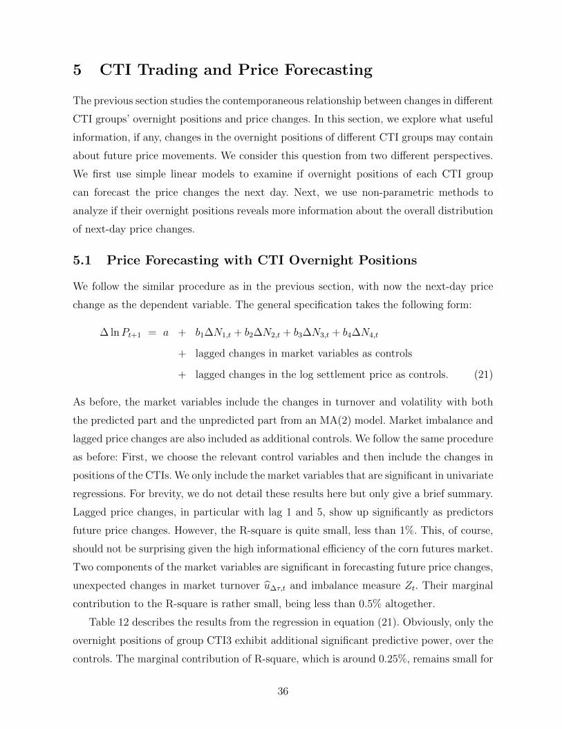
5 CTI Trading and Price Forecasting
The previous section studies the contemporaneous relationship between changes in different
CTI groups’ overnight positions and price changes. In this section, we explore what useful
information, if any, changes in the overnight positions of different CTI groups may contain
about future price movements. We consider this question from two different perspectives.
We first use simple linear models to examine if overnight positions of each CTI group
can forecast the price changes the next day. Next, we use non-parametric methods to
analyze if their overnight positions reveals more information about the overall distribution
of next-day price changes.
5.1 Price Forecasting with CTI Overnight Positions
We follow the similar procedure as in the previous section, with now the next-day price
change as the dependent variable. The general specification takes the following form:
∆ lnPt+1 = a + b1∆N1,t + b2∆N2,t + b3∆N3,t + b4∆N4,t
+ lagged changes in market variables as controls
+ lagged changes in the log settlement price as controls. (21)
As before, the market variables include the changes in turnover and volatility with both
the predicted part and the unpredicted part from an MA(2) model. Market imbalance and
lagged price changes are also included as additional controls. We follow the same procedure
as before: First, we choose the relevant control variables and then include the changes in
positions of the CTIs. We only include the market variables that are significant in univariate
regressions. For brevity, we do not detail these results here but only give a brief summary.
Lagged price changes, in particular with lag 1 and 5, show up significantly as predictors
future price changes. However, the R-square is quite small, less than 1%. This, of course,
should not be surprising given the high informational efficiency of the corn futures market.
Two components of the market variables are significant in forecasting future price changes,
unexpected changes in market turnover u∆τ,t and imbalance measure Zt. Their marginal
contribution to the R-square is rather small, being less than 0.5% altogether.
Table 12 describes the results from the regression in equation (21). Obviously, only the
overnight positions of group CTI3 exhibit additional significant predictive power, over the
controls. The marginal contribution of R-square, which is around 0.25%, remains small for
36

reasons mentioned above. It is interesting to note that this result is consistent with the
results presented in Table 5, which shows that CTI3 is the only group whose overnight
positions are positively correlated across contracts with different maturities. It is also worth
noting that the predictability disappears beyond one day.
Table 12: Regression of the equally weighted price change on lagged changes in overnightposition of each CTI group and lagged change in market variables.
c -0.000 -0.000 -0.000 -0.000 -0.000[-1.211] [-1.244] [-1.194] [-1.791] [-1.386]
∆N1,t -0.061[-0.522]
∆N2,t -0.027[-0.279]
∆N3,t 0.297[2.731]
∆N4,t -0.117[-1.734]
ut,∆τt 0.014 0.014 0.014 0.015 0.014[2.604] [2.599] [2.610] [2.692] [2.586]
Zt 0.013 0.013 0.013 0.012 0.013[2.542] [2.545] [2.541] [2.390] [2.479]
∆ lnPt 0.028 0.028 0.028 0.031 0.033[1.317] [1.288] [1.271] [1.483] [1.517]
∆ lnPt−1 0.010 0.008 0.010 0.007 0.012[0.440] [0.387] [0.435] [0.337] [0.525]
∆ lnPt−2 -0.039 -0.039 -0.039 -0.036 -0.037[-1.772] [-1.770] [-1.779] [-1.649] [-1.700]
∆ lnPt−4 -0.050 -0.050 -0.050 -0.045 -0.048[-2.101] [-2.106] [-2.104] [-1.895] [-2.001]
R2 0.953 0.926 0.920 1.263 1.031
This table presents the regression of the equally weighted price change (∆ lnPt+1) on laggedchanges in overnight position (∆Ni,t) and lagged change in market variables (decomposedinto expected and unexpected parts). The R2 is adjusted by degrees of freedom and inpercentage. The sample period is 1995-2006. The t-statistics are inside brackets. Boldfacemeans significative at the 5% level.
The result that changes in CTI3’s overnight position can predict next day price changes
contrasts interestingly with those from previous work. For Treasury futures, Brandt et al.
(2007) find no significant predicative power for net order flows of different CTI groups
at the daily interval. This may simply reflect the fact that for financial futures, which
are linked to market-wide prices, no CTI group possesses superior information over the
37

market. As mentioned before, this is also a main motivation for us to look at corn futures
in this paper.40 Fishe and Smith (2012) do find floor brokers/traders are over-represented
among the traders who have positive performance on overnight positions. Their results
are consistent with our findings, with two important distinctions. First, market variables
can predict future price changes, as we show here, which implies that expected returns on
futures are time-varying. Thus, positive performance can come from two sources, trading on
time-varying expected returns and on private information. Without properly adjusting the
effect of time-varying expected returns, it is hard to identify the potential effect of private
information. Second, floor brokers and floor traders may have different trading motives
and private information. Pooling them together will prevent us from further identify these
differences. By controlling for the impact of market variables that can predict future price
changes and examining CTI2 and CTI3 groups separately, we are able to better identify
the potential information advantage of group CTI3.
Locke and Onayev (2007) look at 5-minute intervals and find a positive relationship
between price changes and only customer order flows (group CTI4) beyond several lags.
Using weekly trader positions in currency futures, Wang (2004) finds that positions of
speculators (non-commercial traders) have a positive influence on future returns while
positions of hedgers (commercial traders) have a negative influence.41 It should be clear
that the potential information advantage over very short or long horizons documented in
these studies is different from what we identified at daily frequencies (but not beyond).
5.2 Non Parametric Analysis
The regression analysis above focuses on how overnight positions of each CTI group may
forecast next-day price changes, on average. It should be recognized that their positions
may contain other useful information about the next-day price beyond what is capture in
its mean change. It may convey information about other aspects of the next-day price,
such as the distribution of its change. In this section, we use nonparametric statistics to
examine the extent of this information.
First, for each CTI group, we sort the sample into two cases: days when ∆Ni,t > 0
40Dusak (1973), Bessembinder (1992) and de Roon et al. (2000) find different relationships betweenagricultural futures and systematic market risk variables than those for financial futures.
41Using weekly trader positions from the CFTC (commercial and non-commercial) for five foreigncurrency futures markets, January 1993 through March 2010, finds that speculators (non-commercial)positive influence future returns and hedgers (commercial) negatively influence future returns. See alsoBessembinder (1992) and de Roon et al. (2000).
38

and days when ∆Ni,t < 0 (we ignore the days with ∆Ni,t = 0). We then consider the
price change in the following day. If changes in the CTI group’s overnight positions are not
informative about future price changes, we should see the same distribution of next-day
price changes between these two cases. In other words, the distributions of future price
changes conditional on the CTI group’s buying and selling of the market, respectively,
should be the same when these trades are uninformative. Otherwise, the distributions will
be different.
Next, we compare the moments of these two conditional distributions. The first four
rows of panels A to D in Table 13 report the results for CTI group 1 to 4. In particular, we
report in the columns 2 and 3 the the mean, standard deviation, skewness and kurtosis of
the two conditional distributions of ∆ lnPt+1, conditional on buying and selling of a CTI
group on date t. The last column reports the p-value for the test of the null hypothesis
that two conditional moments are the same, i.e., H0 : θ+ = θ−, where θ+ and θ− denote
the moment conditional on buying and selling respectively. Here, the p-value are obtained
using bootstrap statistics with 5,000 simulations.
Consistent with the results from the forecast regressions, the mean of the two con-
ditional distributions are statistically different only for group CTI3. What is interesting
is that the trading of group CTI3 also contains information about the other moments of
future price change. For example, conditional on the buying of group CTI3, the skewness
of the price change the next day is 0.435. But conditional on their selling, the skewness
of the price change the next day becomes −0.067. The difference is significant at the 1%
level. The kurtosis in the two cases are also different, 5.290 for the former and 3.884 for
the latter.
It should also be noted that although the trading of group CTI2 is not informative
about the mean of the future price change, it is informative about its skewness. For both
groups CTI2 and CTI3, buying today predicts a positive skewness for next-day’s price
change, while selling predicts a negative skewness.
Finally, we use the Kolmogorov-Smirnov test (K-S test) to detect the difference between
the two conditional distributions. The results are presented in the last rows of panels A to
D in Table 13 for each CTI group, respectively. We find that the distributions conditional
the buying and selling are different only for group CTI3. We thus conclude that at the CTI
group level, only group CTI3’s trading contains information about future price changes.
It is widely believed among researchers that the CTI3 group consists of mostly hedgers,
39

Table 13: Nonparametric tests on the distribution of future price changes of the equallyweighted price conditional on changes in overnight positions of each CTI group.
∆ lnPt+1
Panel A ∆N1,t > 0 ∆N1,t < 0 p− value (•|+ = •|−)
mean -0.000 -0.000 0.952std 0.013 0.012skewness 0.257 0.178 0.676kurtosis 4.992 4.439 0.322N. obs. 1239 1587
K-S test F+ F− 0.989
Panel B ∆N2,t > 0 ∆N2,t < 0 p− value (•|+ = •|−)
mean -0.000 -0.001 0.531std 0.012 0.013skewness 0.493 -0.044 0.004kurtosis 5.453 4.025 0.009N. obs. 1474 1343
K-S test F+ F− 0.526
Panel C ∆N3,t > 0 ∆N3,t < 0 p− value (•|+ = •|−)
mean 0.000 -0.001 0.001std 0.012 0.013skewness 0.435 -0.067 0.008kurtosis 5.290 3.884 0.012N. obs. 1719 1105
K-S test F+ F− 0.036
Panel D ∆N4,t > 0 ∆N4,t < 0 p− value (•|+ = •|−)
mean -0.001 -0.000 0.075std 0.013 0.013skewness 0.022 0.362 0.077kurtosis 4.102 5.175 0.056N. obs. 1177 1646
K-S test F+ F− 0.421
This tables shows the nonparametric tests on the distribution of future price changes of theequally weighted price (∆ lnPt+1) conditional on changes in overnight positions of each CTIgroup (∆Ni,t, i = 1, 2, 3, 4). Panel A is for CTI1 group, Panel B is for CTI2 group, PanelC is for CTI3 group, and Panel D is for CTI4 group. The K-S test means the Kolmogorov-Smirnov test of the equality of the two conditional future price changes distributions. Thesample period is 1995-2006. The p−values are obtained using bootstrap statistics with 5,000simulations. Bold face means different from zero at the 5% level.
who trade in other products for their own accounts and use the futures for hedging reasons.
For example, Ferguson and Mann (1999) states that “Trades executed on behalf of other
40
members (CTI3) are most often trades done for hedging purposes.”42 Such a perception
has lead most prior work to assume that group CTI3 does not possess superior informa-
tion, at least beyond very short horizons (e.g., several minutes). It was then often bundled
either with group CTI2 as hedgers or with CTI1 as floor broker/traders (FBT). Even
though Fishe and Smith (2012) have find a more likely positive correlation between the
overnight positions of FBTs as a group, they interpret this information advantage as com-
ing from better understanding order flows rather coming from private information about
more fundamental factors.43 Our analysis suggests that group CTI3 may have a distinctive
information advantage over other groups at daily horizons. This information is unlikely to
come from overall order flows, for which group CTI1 not CTI3 is in the best position to
observe.44 Thus, group CTI3 may play a unique role in the futures market, especially in
bringing in information in the price formation process. It would be interesting to further
explore the potential source of this information.
6 Conclusion
In this paper, we examine the trading behavior of different CTI groups in the corn futures
market. Despite the fact that each group consists of a rich set of market participants with
potentially different trading motives, we have several interesting findings. First, there are
clear differences in the trading behavior of the different CTI groups. In particular, most of
the trading volume is attributed to the trading of groups CTI1 and CTI4. In addition, most
of their volume is intraday. In terms of interday trading, it is coming mostly from groups
CTI2 and CTI3. This is consistent with the broad definition of each CTI group. Group
CTI4 is the main liquidity demander, especially on intraday basis, while group CTI1 is the
main liquidity supplier. Groups CIT2 and CTI3 trade mostly for hedging or speculative
reasons. The half life of their positions tend to be longer—they carry non-trivial amount
of overnight positions.
Consistent with this picture, we observe that on intraday trading, group CTI4 con-
sistently loses money, which reflects the price they pay for consuming liquidity. On the
42See also Manaster and Mann (1996). Both papers further attribute the hedging needs to the deltahedging of CTI3 traders’ positions in futures options.
43As mentioned above, Fishe and Smith (2012)’s results on positive performance from overnight positionsof FBTs may come from risk-taking rather than better information.
44In fact, Dewally et al. (2013) actually show that the group composed of market makers and floortraders, based on CFTC’s LTRS data, on average lose money on their overnight positions.
41

contrary, group CTI1 consistently makes money on their intraday trading, which reflects
the compensation for their liquidity provision. The Sharpe ratio for group CTI1’s intra-
day liquidity provision amounts to 0.791, which is quite substantial. Furthermore, we find
that group CTI1 P&L from intraday trading is positively correlated with the unexpected
change in turnover and high minus low price, which captures the intraday price volatility.
These results are consistent with the interpretation that their P&L compensates for the
risk of market making.
The different trading behavior of different CTI groups further allow us to examine
their role in the price discovery process of the market. Here, we find several informative
results. First, we noticed that daily changes in several market variables, especially the
expected level of turnover and unexpected change in high minus low price during the day,
are significantly correlated with contemporaneous changes in price. More importantly, we
find that a measure of trade imbalance, a normalized difference between volume at the
top price interval and the bottom price interval, exhibits significant explanatory power on
contemporaneous price changes. Its contribution to R-square exceed 15%, while the other
variables including lagged price changes can only yield a R-square of no more than 1.5%
even when they are statistically significant. Next, we show that changes in the interday
positions of only groups CTI2 and CTI4 also have significant explanatory power for the
contemporaneous price. The former has a negative coefficient, indicating that they trade
against the market, while the latter has a positive coefficient. When we include both
changes in the regression, only changes in the interday positions of group CTI4 remains
significant, with a positive coefficient. In other words, when group CTI4 collectively buys
during a day, the futures price tends to increase for the same day.
We further explore if changes in the overnight positions of different CTI groups can
predict future price changes. We find that only the changes in group CTI3’s interday
positions can predict the change in futures price next day. In addition, using nonparametric
statistics, we also find that group CTI3’s interday positions contains information about
other aspects of the distribution of next-day price changes such as skewness and kurtosis.
Overall, we conclude that in the corn futures market, group CTI1 mainly act as market
makers for intraday transactions. Groups CTI2 and CTI4 contribute to the price discovery
through their intraday trading. Group CTI3, however, may possess private information
about futures prices beyond the intraday horizon.
42

References
Bessembinder, H. (1992). Systematic risk, hedging pressure, and risk premiums in futuresmarekts. Review of Financial Studies 5, 4, 637–667.
Bessembinder, H. and K. Chan (1992). Time-varying risk premia and forecastable returnsin futures markets. Journal of Financial Economics 32, 2, 169–193.
Bessembinder, H. and P. J. Seguin (1993). Price Volatility, Trading Volume, and Mar-ket Depth: Evidence from Futures Markets. Journal of Financial and QuantitativeAnalysis 28, 21–39.
Black, F. (1976). The pricing of commodity contracts. Journal of Financial Economics 3,167–179.
Boyd, N. E. and A. Kurov (2012). Trader survival: evidence from the energy futuresmarkets. Journal of Futures Markets 32, 9, 809 – 836.
Brandt, M. W., K. A. Kavajecz, and S. E. Underwood (2007). Price Discovery in theTreasury Futures Markets. The Journal of Futures Markets 27, 11, 1021–1051.
Brunetti, C., B. Buyuksahin, and J. H. Harris (2011). Speculators, prices and marketvolatility. mimeo, http://ssrn.com/abstract=1736737 -, 1–34.
Buyuksahin, B. and J. H. Harris (2011). Do speculators drive curde oil futures prices? TheEnergy Journal 32, 2, 167–202.
Chang, E. C. (1985). Returns to speculators and the theory of normal backwardation.Journal of Finance 40, 1, 193–208.
Daigler, R. T. and M. K. Wiley (1999). The Impact of Trader Type on the FuturesVolatility Volume Relation. Journa of Finance Volume 54, 6, December, 2297–2316.
de Roon, F., T. E. Nijman, and C. Veld (2000). Hedging pressure effects in futures markets.Journal of Finance 55, 3, 1437–1456.
Dewally, M., L. H. Ederington, and C. S. Fernando (2013). Determinants of Trader Profitsin Commodity Futures Markets. Review of Financials Studies 26, 10, 2648–2683.
Dusak, K. (1973). Futures trading and investors returns: an investigation of commoditymarket risk premiums. Journal of Political Economy 81, 6, 1387–1406.
Ederington, L. and J. H. Lee (2002). Who Trades Futures and How: Evidence from theHeating Oil Futures Market. Journal of Business 75, 2, 353 – 373.
Erb, C. B. and C. R. Harvey (2006). The strategic and tactical value of commodity futures.Financial Analysts Journal 62, 2, 69–97.
Evans, M. D. D. and R. K. Lyons (2002). Order flow and exchange rate dynamics. Journalof Political Economy 110, 1, 170–180.
Ferguson, M. and S. C. Mann (1999). The Impact of Off-Exchange Customer Trades onPrices: Evidence from the Futures Markets. Working paper .
Fishe, R. P. H. and A. D. Smith (2012). Identifying informed traders in futures markets.Journal of Financial Markets 15, 329 – 359.
43

Fishman, M. J. and F. A. Longstaff (1992). Dual trading in futures markets. Journal ofFinance 47, 2, 643 – 671.
Gorton, G. and K. G. Rouwenhorst (2006). Facts and fantasies about commodity futures.Financial Analysts Journal 62, 2, 47–68.
Gorton, G. B., F. Hayashi, and K. G. Rouwenhorst (2013). The fundamentals of commodityfutures returns. Review of Finance 17, 1, 35–105.
Graman, M. and M. J. Klass (1980). On the estimation of security price volatilities fromhistorical data. Journal of Business 53, 67–78.
Grossman, S. (1976). On the efficiency of competitive stock markets where trades havediverse information. Journal of Finance 31, 2, 573–585.
Grossman, S. J. and M. H. Miller (1988). Liquidity and Market Structure. Journal ofFinance 43, 3, 617–633.
Grossman, S. J. and J. E. Stiglitz (1980). On the impossibility of informationally efficientmarkets. The American Economic Review 70, 3, 393–408.
Haigh, M. S., J. Hranaiova, and J. A. Overdahl (2005). Price dynamics, price discoveryand large futures trader interactions in the energy complex. U.S. CFTC Workingpaper -, 1–44.
Hamilton, J. D. and J. C. Wu (2015). Effects of index-fund inveting on commodity futuresprices. International Economic Review 56, 1, 187–205.
Hartzmark, M. L. (1987). Returns to individual traders of futures: aggregate results.Journal of Political Economy 95, 6, 1292–1306.
Hartzmark, M. L. (1991). Luck versus forecast ability: dedeterminants of trader perfor-mance in futures markets. Journal of Business 64, 1, 49–74.
Hicks, J. R. (1939). Value and Capital. Oxford University Press.
Hirshleifer, D. (1988). Residual risk, trading costs, and commodity futures risk premia.Review of Financial Studies 1, 2, 173–193.
Hirshleifer, D. (1989). Determinants of hedging and risk premia in commodity futuresmarkets. Journal of Financial and Quantitative Analysis 24, 3, 313–331.
Hong, H. and M. Yogo (2012). What does futures market interest tell us about the macroe-conomy and asset prices? Journal of Financial Economics 105, 473–490.
Houthakker, H. S. (1957). Can speculators forecast prices? Review of Economics andStatistics 39, 2, 143–151.
Kaldor, N. (1939). Speculation and economic stability. Review of Economics Studies 7, 1,1–27.
Kang, W., K. G. Rouwenhorst, and K. Tang (2014). The role of hedgers andspeculators in liquidity provision to commoditty futures markets. mimeo,http://ssrn.com/abstract=2449315 -, 1–53.
Keynes, J. M. (1923). “Some aspects of commodity markets”. Manchester Guardian Com-mercial, Reconstruction Supplement. In The Collected Writings of John Maynard
44

Keynes, Vol. 12. London: Macmillan.
Kucher, O. and A. Kurov (2014). Business cycle, storage, and energy prices. Review ofFinancial Economics 23, 217–226.
Kurov, A. (2008). Information and noise in financial markets: evidence from the E-miniindex futures. The Journal of Financial Research Fall, 31, 3, 247–270.
Kurov, A. and D. J. Lasser (2004). Price dynamics in the regular and E-mini futuresmarkets. Journal of Financial and Quantitative Analysis 39, 2, 365–384.
Kuserk, G. J. and P. R. Locke (1993). Scalper bebehavior futures markets: an empiricalanalysis. Journal of Futures Markets 13, 4, 409–431.
Kyle, A. S. (1985). Continuous auctions and insider trading. Econometrica 53, 6, 1315–1336.
Labuszewski, J., J. E. Nyhoff, R. Co, and P. Peterson (2010). The CME group risk man-agement handbook, products and applications. John Wiley and Sons, Inc.
Leuthold, R. M., P. Garcia, and R. Lu (1994). The returns and forecasting ability of largetraders in the forzen pork bellies futures market. Journal of Business 67, 3, 459–473.
Leuthold, R. M. and M.-K. Kim (2000). Managing Overnight Corn Price Risks: E*Hedgingversus Tokyo. Journal of Agribusiness 18, 3, 275 – 288.
Locke, P. and Z. Onayev (2007). Order flow, dealer profitability, and price formation.Journal of Financial Economics 85, 857–887.
Manaster, S. and S. Mann (1996). Life in the pits: competitive market making and inven-tory control. Review of Financial Studies 9, 953–975.
Manaster, S. and S. C. Mann (1999). Sources of Market Making Profits: Man Does NotLive by Spread Alone. working paper .
Menkveld, A. J., A. Sarkar, and M. van der Wel (2012). Customer order flow, intere-mediaries, and discovery of the equilibrium risk-free rate. Journal of Financial andQuantitative Analysis 47, 4, 821–849.
Rouwenhorst, K. G. and K. Tang (2012). Commodity investing. Annual Review of Finan-cial Economics 4, 447–467.
Sanders, D. R., S. H. Irwin, and R. P. Merrin (2009). Smart money: the forecasting abilityof CFTC large traders in agricultural futures markets. Journal of Agricultural andResource Economics 34, 2, 276–296.
Silber, W. L. (1984). Marketmarket behavior in an auction market: an analysis of scalpersin futures markets. Journa of Finance 39, 937–953.
Singleton, K. J. (2014). Investor flows and the 2008 boom/bust in oil prices. ManagementScience 60, 2, 300–318.
Stoll, H. R. (1979). Commodity futures and spot price determiantion and hedging incapital market equilibrium. Journal fo Financial and Quantitative Analysis 14, 4,873–895.
Strong, R. A. (2009). Portfolio Construction, Management, and Protection (5th edition).
45

South Western Cengage Learning.
Vayanos, D. and J. Wang (2012). Theories of Liquidity. Foundations and Trends inFinance 6, 221–317.
Wang, C. (2003). The behavior and performance of major types of futures traders. Journalof Futures Markets 23, 1–31.
Wang, C. (2004). Futures trading activity and predictable foreign exchange market move-ments. Journal of Banking and Finance 28, 1023–1041.
Wang, J. (1994). A model of competitive stock trading volume. Journal of PoliticalEconomy 102, 1, 127–168.
Wiley, M. K. and R. T. Daigler (1998). Volume relationships among types of traders inthe financial futures markets. Journal of Futures Markets 18, 91–113.
Working, H. (1949). The theory of price storage. American Economic Review 39, 6,1254–1262.
46

A Appendix
A.1 Volume from EOD and LDB files
This section presents the differences between the daily total volume from the EOD and LDB
data files. Figure A.1 Panel (a) presents the EOD volume, Panel (b) the LDB volume, Panel
(c) present the difference between both volumes and Panel (d) the difference normalized
by the the daily open interest. Table A.1 presents the descriptive statistics of the graphs
in Figure A.1.
1995 1996 1997 1998 1999 2000 2001 2002 2003 2004 2005 20060
50
100
150
200
250
300
Dates
Vt,
eod (t
hous
and
cont
ract
s)
1995 1996 1997 1998 1999 2000 2001 2002 2003 2004 2005 20060
50
100
150
200
250
300
Dates
Vt,
ldb (t
hous
and
cont
ract
s)
(a) (b)
1995 1996 1997 1998 1999 2000 2001 2002 2003 2004 2005 20060
50
100
150
200
250
300
Dates
Vt,
eod −
Vt,
ldb (t
hous
and
cont
ract
s)
1995 1996 1997 1998 1999 2000 2001 2002 2003 2004 2005 20060
50
100
150
200
250
300
Dates
(Vt,
eod −
Vt,
ldb)/O
t (%)
(c) (d)
Figure A.1: Daily market volume comparison between EOD volume and LDB volume.This figure shows the differences between the reported market volume in the EOD files andthe market volume calculated from LDB files. Panel (a) present the total market volumein thousand contracts from the EDO files, Panel (b) the total market volume in thousandcontracts calculated from the LDB files, Panel (c) difference between EDO and LDB volumesin thousand contracts and Panel (d) the difference between EOD and LDB volume as apercentage of the total open interest, respectively.
The numbers in the LDB files are made public by CBOT after the second reconcilia-
tion of the unmatched trades. There is some controversy about how many un-reconciliated
trades are missing. CBOT says that 90% of the out trades are cleared in the second rec-
onciliation (Strong (2009), pp.580). Taking into account these references and the numbers
47

in Table A.1, we conclude that in the LDB files about 31% of the total EOD volume is
missing, or 5% in terms of Open Interest. As it was pointed in the main text the correlation
between both volume measures (EOD and LDB) is 0.983.
Table A.1: Descriptive statistics for the total market volume figures either from the Endof Day (EOD) files or from the Liquidity Data Bank (LDB) files.
mean median std skew kurt
Vt,EOD/1000 74.048 65.676 35.373 1.667 7.849
Vt,LDB/1000 51.112 45.778 23.553 1.575 7.310
(Vt,EOD − Vt,LDB)/1000 22.936 17.833 17.667 2.621 16.754
(Vt,EOD − Vt,LDB)/OIt(%) 5.053 4.325 3.277 1.870 9.968
This table presents the descriptive statistics for the total market volume figures either fromthe End of Day (EOD) files or from the Liquidity Data Bank (LDB) files. The figures aremeasured in number of contracts. The sample period is 1995-2006.
As mentioned in the text, for the period from January 2, 2003 to the end of our sample,
May 8, 2006, CBOT also provided us the data on electronic and spread volume. Table A.2
shows the mean daily contracts traded on each venue during these last years of the sample.
The numbers are mean daily trading contracts in thousands.
Table A.2: Mean daily contracts traded in the EOD file and LDB files broken by venueand type of trade.
mean
Vt,EOD (in thousands) 93.948
Vt,LDB (in thousands) 66.386
Vt, no spread-LDB-pit (in thousands) 61.659
Vt, no spread-LDB-electro (in thousands) 1.496
Vt, spread-LDB-pit (in thousands) 2.319
Vt, spread-LDB-electro (in thousands) 0.912
(Vt,EOD − Vt, no-spread-LDB-pit) (in thousands) 32.289
(Vt,EOD − Vt, no-spread-LDB-pit)/OIt (%) 5.226
This table presents the descriptive statistics for the total market volume figures either fromthe End of Day (EOD) files or from the Liquidity Data Bank (LDB) files broken by venue(pit vs. electronic) and type of trade (no spread vs. spread). The figures are measured innumber of contracts. The sample period is 1995-2006.
48

A.2 CTI Definitions
The following CTI definitions were taken from the CBOT web site before it merged with
the CME to form the CME Group. They correspond to what was rule number 332.03 in
the CBOT Rule Book. Now the CTI definitions are in Rule 536.D on the Rule Book of
the CME Group (see www.cmegroup.com web site).
RULE 332.03 Customer Type Indicator (CTI) Codes.45 Each clearing member must
identify each transaction executed on the Floor of the Exchange or on e-cbot, on the record
of transactions that is submits to the Clearing Services Provider, with the correct customer
type indicator (CTI) code. The CTI codes are as follows:
CTI1: Electronic Trading and Open Auction: Applies to transactions initiated and
executed by an individual member for his/her own account, for an account he/she
controls, or for an account in which he/she has an ownership or financial interest.
However, transactions initiated and executed by a member for the proprietary ac-
count of a member firm must be designated as CTI2 transactions.
CTI2: Electronic Trading and Open Auction Applies to orders entered/trades exe-
cuted for the proprietary accounts of a member firm or Qualified Affiliate, as defined
in Regulations 230.02 or 230.03. Members initiating and executing trades by open
auction for the proprietary accounts of a member firm may participate in the Ex-
change CTI 2/1 Conversion Program.
CTI3: Electronic Trading Applies to orders entered by a member or a non-member
Registered User for the account of another individual member or an account con-
trolled by such other individual member.
CTI3: Open Auction Applies to orders that a member executes on behalf of another
individual member, or for an account such other member controls or in which such
other member has an ownership or financial interest.
CTI4: Electronic Trading and Open Auction Applies to all orders/transactions not
included in CTI categories 1, 2, or 3. These typically are orders entered by or on
behalf of non-member entities.
45Source: CBOT Rules, www.cbot.com.
49

As it was already said in the main text, on December 1st, 2004, took place the agreement
among the Exchanges and the National Futures Association to “Harmonize the set of
CTI code definitions for the industry.” The main differences from the previous CBOT
classification was:
� CTI2 includes all trades from proprietary account. Previously it was exclusively
reserved for the proprietary account of clearing members. It will also include members
receiving preferential rates for their trading, they were previously classified as CTI4.
� CTI3 will also include open outcry orders entered for a member’s account through
the normal customer order flow process, previously they were coded as CTI4.
That means that after December 1, 2004, some of the trades previously coded in the
open outcry trading as CTI4, afterward they were coded either as CTI2 or CTI3.
A.3 Dynamics of Market Variables and P&L
As shown in Table 1, changes in market variables such as turnover and normalized high
minus low prices, exhibit significant persistence. Table A.3 presents the MA(2) estimation
of the these variables and Table A.4 present the characteristics of the residuals in the
MA(2) estimation.
Table A.3: Parameter estimates for market variables.
c θ1 θ2 R2
∆τt -0.000 -0.698 -0.156 31.411[-0.035] [-26.006] [-6.333]
∆Xt 0.000 -0.828 -0.016 40.567[0.018] [-35.299] [-0.699]
This table presents the parameter estimates for changes in market variables using a MA(2)model. The sample period is 1995-2006. The t-statistics are inside brackets. Bold face meanssignificative at the 5% level.
Table A.5 presents the correlations among the residuals of the MA(2) for the market
variables.
As noted in the main text, given the persistence in P&L, we consider changes in P&L,
which still exhibits non-trivial autocorrelation. Following the same approach as for the
market variables, we decompose the changes in P&L into a predictable part using an
50
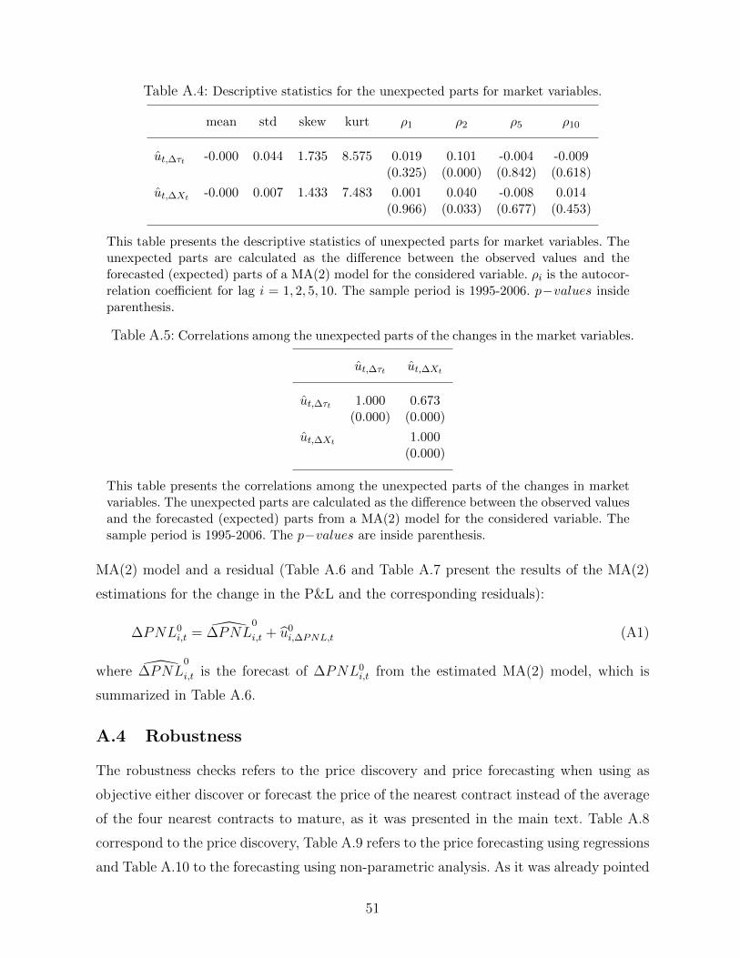
Table A.4: Descriptive statistics for the unexpected parts for market variables.
mean std skew kurt ρ1 ρ2 ρ5 ρ10
ut,∆τt -0.000 0.044 1.735 8.575 0.019 0.101 -0.004 -0.009(0.325) (0.000) (0.842) (0.618)
ut,∆Xt -0.000 0.007 1.433 7.483 0.001 0.040 -0.008 0.014(0.966) (0.033) (0.677) (0.453)
This table presents the descriptive statistics of unexpected parts for market variables. Theunexpected parts are calculated as the difference between the observed values and theforecasted (expected) parts of a MA(2) model for the considered variable. ρi is the autocor-relation coefficient for lag i = 1, 2, 5, 10. The sample period is 1995-2006. p−values insideparenthesis.
Table A.5: Correlations among the unexpected parts of the changes in the market variables.
ut,∆τt ut,∆Xt
ut,∆τt 1.000 0.673(0.000) (0.000)
ut,∆Xt 1.000(0.000)
This table presents the correlations among the unexpected parts of the changes in marketvariables. The unexpected parts are calculated as the difference between the observed valuesand the forecasted (expected) parts from a MA(2) model for the considered variable. Thesample period is 1995-2006. The p−values are inside parenthesis.
MA(2) model and a residual (Table A.6 and Table A.7 present the results of the MA(2)
estimations for the change in the P&L and the corresponding residuals):
∆PNL0i,t = ∆PNL
0
i,t + u0i,∆PNL,t (A1)
where ∆PNL0
i,t is the forecast of ∆PNL0i,t from the estimated MA(2) model, which is
summarized in Table A.6.
A.4 Robustness
The robustness checks refers to the price discovery and price forecasting when using as
objective either discover or forecast the price of the nearest contract instead of the average
of the four nearest contracts to mature, as it was presented in the main text. Table A.8
correspond to the price discovery, Table A.9 refers to the price forecasting using regressions
and Table A.10 to the forecasting using non-parametric analysis. As it was already pointed
51

Table A.6: Parameter estimates for the change in the intraday P&L for the groups CTI1and CTI4.
c θ1 θ2 R2
∆PNL01,t 0.006 -0.855 -0.062 42.443
[0.114] [-28.667] [-2.257]
∆PNL04,t -0.011 -0.936 -0.009 46.650
[-0.239] [-35.046] [-0.413]
This table presents the parameter estimates from a MA(2) model for the change in theintraday P&L for the groups CTI1 and CTI4 (∆PNL0
i,t, i = 1, 4). The R2 is adjusted bydegrees of freedom and in percentage. The sample period is 1995-2006. The t-statistics areinside brackets.Table A.7: Descriptive statistics for the unexpected parts of the changes in the intradayP&L of groups CTI1 and CTI4.
mean std skew kurt ρ1 ρ2 ρ5 ρ10
u0t,∆PNL1,t
-0.012 33.374 2.585 26.755 -0.001 -0.011 -0.008 0.015
(0.963) (0.561) (0.688) (0.431)
u0t,∆PNL4,t
0.006 41.834 -2.378 26.931 0.000 0.007 0.051 0.006
(0.998) (0.712) (0.006) (0.759)
This table presents the descriptive statistics of the unexpected parts of the changes in theintraday P&L of groups CTI1 and CTI4 (u0
t,∆PNLi,t, i = 1, 4). ρi is the autocorrelation
coefficient for lag i = 1, 2, 5, 10. The sample period is 1995-2006. p-values are inside paren-thesis.
the conclusions do not change.
52
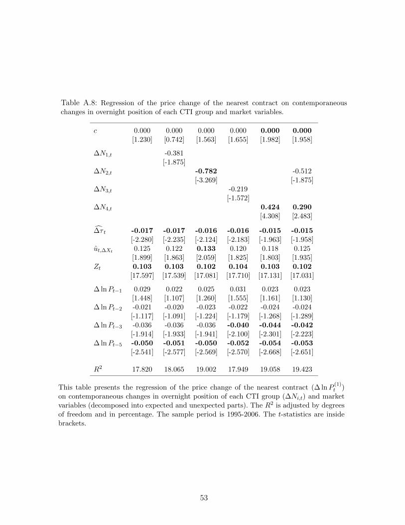
Table A.8: Regression of the price change of the nearest contract on contemporaneouschanges in overnight position of each CTI group and market variables.
c 0.000 0.000 0.000 0.000 0.000 0.000[1.230] [0.742] [1.563] [1.655] [1.982] [1.958]
∆N1,t -0.381[-1.875]
∆N2,t -0.782 -0.512[-3.269] [-1.875]
∆N3,t -0.219[-1.572]
∆N4,t 0.424 0.290[4.308] [2.483]
∆τ t -0.017 -0.017 -0.016 -0.016 -0.015 -0.015[-2.280] [-2.235] [-2.124] [-2.183] [-1.963] [-1.958]
ut,∆Xt 0.125 0.122 0.133 0.120 0.118 0.125[1.899] [1.863] [2.059] [1.825] [1.803] [1.935]
Zt 0.103 0.103 0.102 0.104 0.103 0.102[17.597] [17.539] [17.081] [17.710] [17.131] [17.031]
∆ lnPt−1 0.029 0.022 0.025 0.031 0.023 0.023[1.448] [1.107] [1.260] [1.555] [1.161] [1.130]
∆ lnPt−2 -0.021 -0.020 -0.023 -0.022 -0.024 -0.024[-1.117] [-1.091] [-1.224] [-1.179] [-1.268] [-1.289]
∆ lnPt−3 -0.036 -0.036 -0.036 -0.040 -0.044 -0.042[-1.914] [-1.933] [-1.941] [-2.100] [-2.301] [-2.223]
∆ lnPt−5 -0.050 -0.051 -0.050 -0.052 -0.054 -0.053[-2.541] [-2.577] [-2.569] [-2.570] [-2.668] [-2.651]
R2 17.820 18.065 19.002 17.949 19.058 19.423
This table presents the regression of the price change of the nearest contract (∆ lnP(1)t )
on contemporaneous changes in overnight position of each CTI group (∆Ni,t) and marketvariables (decomposed into expected and unexpected parts). The R2 is adjusted by degreesof freedom and in percentage. The sample period is 1995-2006. The t-statistics are insidebrackets.
53

Table A.9: Regression of the nearest price change on lagged changes in position and laggedchanges in market variables.
c -0.000 -0.000 -0.000 -0.001 -0.000[-1.422] [-1.399] [-1.409] [-1.953] [-1.606]
∆N1,t -0.013[-0.100]
∆N2,t -0.012[-0.109]
∆N3,t 0.306[2.592]
∆N4,t -0.138[-1.904]
ut,∆τ 0.015 0.015 0.015 0.016 0.015[2.533] [2.532] [2.532] [2.615] [2.511]
Zt 0.014 0.014 0.014 0.013 0.014[2.585] [2.585] [2.584] [2.442] [2.522]
∆ lnPt 0.052 0.052 0.052 0.055 0.057[2.435] [2.428] [2.382] [2.585] [2.621]
∆ lnPt−1 0.004 0.004 0.004 0.002 0.006[0.180] [0.171] [0.178] [0.074] [0.264]
∆ lnPt−2 -0.035 -0.035 -0.035 -0.033 -0.034[-1.627] [-1.628] [-1.630] [-1.518] [-1.560]
∆ lnPt−4 -0.052 -0.052 -0.052 -0.047 -0.049[-2.288] [-2.288] [-2.290] [-2.081] [-2.177]
R2 1.229 1.194 1.194 1.504 1.328
This table presents the regression of the nearest price change (∆ lnP(1)t+1) on lagged changes
in position (∆Ni,t) and lagged changes in market variables (decomposed into expected andunexpected parts). The R2 is adjusted by degrees of freedom and in percentage. The sampleperiod is 1995-2006. The t-statistics are inside brackets.
54

Table A.10: Nonparametric tests on the distribution of future price changes of the nearestcontract conditional on changes in overnight positions of each CTI group.
∆ lnPt+1
Panel A ∆N1,t > 0 ∆N1,t < 0 p− value (•|+ = •|−)
mean -0.000 -0.001 0.625std 0.014 0.013skewness 0.196 0.126 0.740kurtosis 5.361 4.328 0.089N. obs. 1239 1587
K-S test F+ F− 0.559
Panel B ∆N2,t > 0 ∆N2,t < 0 p− value (•|+ = •|−)
mean -0.000 -0.001 0.654std 0.013 0.014skewness 0.394 -0.055 0.030kurtosis 5.175 4.544 0.305N. obs. 1474 1343
K-S test F+ F− 0.602
Panel C ∆N3,t > 0 ∆N3,t < 0 p− value (•|+ = •|−)
mean 0.000 -0.001 0.002std 0.013 0.014skewness 0.428 -0.161 0.005kurtosis 5.316 4.172 0.070N. obs. 1719 1105
K-S test F+ F− 0.043
Panel D ∆N4,t > 0 ∆N4,t < 0 p− value (•|+ = •|−)
mean -0.001 -0.000 0.053std 0.014 0.013skewness -0.076 0.358 0.043kurtosis 4.406 5.203 0.200N. obs. 1177 1646
K-S test F+ F− 0.349
This table shows the nonparametric tests on the distribution of future price changes of
the nearest contract (∆ lnP(1)t+1) conditional on changes in overnight positions of each CTI
group(∆Ni,t, i = 1, 2, 3, 4). Panel A is for CTI1 group, Panel B is for CTI2 group, PanelC is for CTI3 group, and Panel D is for CTI4 group. The K-S test means the Kolmogorov-Smirnov test of the equality of the two conditional future price changes distributions. Thep−values are obtained using bootstrap statistics with 5,000 simulations. Bold face meansdifferent from zero at the 5% level. The sample period is 1995-2006.
55