Tradeoffs between synchronization, communication,

and work in parallel linear algebra computations

Edgar SolomonikErin CarsonNicholas KnightJames Demmel

Electrical Engineering and Computer SciencesUniversity of California at Berkeley

Technical Report No. UCB/EECS-2014-8

http://www.eecs.berkeley.edu/Pubs/TechRpts/2014/EECS-2014-8.html

January 25, 2014

Report Documentation Page Form ApprovedOMB No. 0704-0188

Public reporting burden for the collection of information is estimated to average 1 hour per response, including the time for reviewing instructions, searching existing data sources, gathering andmaintaining the data needed, and completing and reviewing the collection of information. Send comments regarding this burden estimate or any other aspect of this collection of information,including suggestions for reducing this burden, to Washington Headquarters Services, Directorate for Information Operations and Reports, 1215 Jefferson Davis Highway, Suite 1204, ArlingtonVA 22202-4302. Respondents should be aware that notwithstanding any other provision of law, no person shall be subject to a penalty for failing to comply with a collection of information if itdoes not display a currently valid OMB control number.

1. REPORT DATE 25 JAN 2014 2. REPORT TYPE

3. DATES COVERED 00-00-2014 to 00-00-2014

4. TITLE AND SUBTITLE Tradeoffs between synchronization, communication, and work in parallellinear algebra computations

5a. CONTRACT NUMBER

5b. GRANT NUMBER

5c. PROGRAM ELEMENT NUMBER

6. AUTHOR(S) 5d. PROJECT NUMBER

5e. TASK NUMBER

5f. WORK UNIT NUMBER

7. PERFORMING ORGANIZATION NAME(S) AND ADDRESS(ES) University of California at Berkeley,Electrical Engineering andComputer Sciences,Berkeley,CA,94720

8. PERFORMING ORGANIZATIONREPORT NUMBER

9. SPONSORING/MONITORING AGENCY NAME(S) AND ADDRESS(ES) 10. SPONSOR/MONITOR’S ACRONYM(S)

11. SPONSOR/MONITOR’S REPORT NUMBER(S)

12. DISTRIBUTION/AVAILABILITY STATEMENT Approved for public release; distribution unlimited

13. SUPPLEMENTARY NOTES

14. ABSTRACT This paper derives tradeoffs between three basic costs of a parallel algorithm: synchronization, datamovement, and computational cost. Our theoretical model counts the amount of work and data movementas a maximum of any execution path during the parallel computation. By considering this metric, ratherthan the total communication volume over the whole machine, we obtain new insight into thecharacteristics of parallel schedules for algorithms with non-trivial dependency structures. The tradeoffswe derive are lower bounds on the execution time of the algorithm which are independent of the number ofprocessors, but dependent on the problem size. Therefore, these tradeoffs provide lower bounds on theparallel execution time of any algorithm computed by a system composed of any number of homogeneouscomponents each with associated computational, communication, and synchronization payloads. We firststate our results for general graphs, based on expansion parameters, then we apply the theorem to anumber of specific algorithms in numerical linear algebra, namely triangular substitution, Gaussianelimination, and Krylov subspace methods. Our lower bound for LU factorization demonstrates theoptimality of Tiskin?s LU algorithm [24] answering an open question posed in his paper, as well as of the2.5D LU [20] algorithm which has analogous costs. We treat the computations in a general manner bynoting that the computations share a similar dependency hypergraph structure and analyzing thecommunication requirements of lattice hypergraph structures.

15. SUBJECT TERMS

16. SECURITY CLASSIFICATION OF: 17. LIMITATION OF ABSTRACT Same as

Report (SAR)

18. NUMBEROF PAGES

19

19a. NAME OFRESPONSIBLE PERSON

a. REPORT unclassified

b. ABSTRACT unclassified

c. THIS PAGE unclassified

Standard Form 298 (Rev. 8-98) Prescribed by ANSI Std Z39-18

Copyright © 2014, by the author(s).All rights reserved.

Permission to make digital or hard copies of all or part of this work forpersonal or classroom use is granted without fee provided that copies arenot made or distributed for profit or commercial advantage and that copiesbear this notice and the full citation on the first page. To copy otherwise, torepublish, to post on servers or to redistribute to lists, requires prior specificpermission.

Tradeoffs between synchronization, communication, and work in parallellinear algebra computations

Edgar Solomonik, Erin Carson, Nicholas Knight, and James Demmel

Department of EECS, University of California, Berkeley

January 25, 2014

Abstract

This paper derives tradeoffs between three basic costs of a parallel algorithm: synchronization, data movement, and computationalcost. Our theoretical model counts the amount of work and data movement as a maximum of any execution path during the parallelcomputation. By considering this metric, rather than the total communication volume over the whole machine, we obtain new insightinto the characteristics of parallel schedules for algorithms with non-trivial dependency structures. The tradeoffs we derive are lowerbounds on the execution time of the algorithm which are independent of the number of processors, but dependent on the problem size.Therefore, these tradeoffs provide lower bounds on the parallel execution time of any algorithm computed by a system composed of anynumber of homogeneous components each with associated computational, communication, and synchronization payloads. We first stateour results for general graphs, based on expansion parameters, then we apply the theorem to a number of specific algorithms in numericallinear algebra, namely triangular substitution, Gaussian elimination, and Krylov subspace methods. Our lower bound for LU factorizationdemonstrates the optimality of Tiskin’s LU algorithm [24] answering an open question posed in his paper, as well as of the 2.5D LU [20]algorithm which has analogous costs. We treat the computations in a general manner by noting that the computations share a similardependency hypergraph structure and analyzing the communication requirements of lattice hypergraph structures.

1 IntroductionWe model a parallel machine as a network of processors which communicate by point-to-point messages. This model has three basicarchitectural parameters,

• α – network latency (time) for a message between a pair of processors,

• β – time to inject a word of data into (or extract it from) the network,

• γ – time to perform a floating point operation on local data,

which are associated with three algorithmic costs,

• S – number of messages sent (network latency cost / synchronization cost),

• W – number of words of data moved (bandwidth cost / communication cost),

• F – number of local floating point operations performed (computational cost).

We describe our execution schedule model and show how S, W , and F are measured in any schedule in Section 2. Each quantityis accumulated along some path of dependent executions in the schedule. The sequence of executions done locally by any processorcorresponds to one such path in the schedule, so our costs are at least as large as those incurred by any single processor during theexecution of the schedule. The parallel execution time of the schedule is closely proportional to these three quantities, namely,

max(S · α,W · β, F · γ) ≤ execution time ≤ S · α+W · β + F · γ.

Since our analysis will be asymptotic, we do not consider overlap between communication and computation and are able to measure thethree quantities separately. Our model is similar to the LogP model [7] with L = α, o = g = β, and no network capacity constraint.

Our theoretical analysis also precludes recomputation within a parallelization of an algorithm, as we associate an algorithm with aset of vertices, each of which is a computation, and assign them to unique processors. However, a parallel algorithm which employsrecomputation has a different dependency graph structure, to which our analysis may subsequently be applied. While there are manyexisting parallel algorithms for the applications we explore that employ recomputation, to the best of our knowledge none of themperform less communication than ascribed by the recomputation-excluding lower bounds we present.

We reason about parallel algorithms by considering the dependency graphs of certain computations. We will first derive theoreticalmachinery for obtaining lower bounds on dependency graphs with certain expansion parameters and then show how this result yields

1

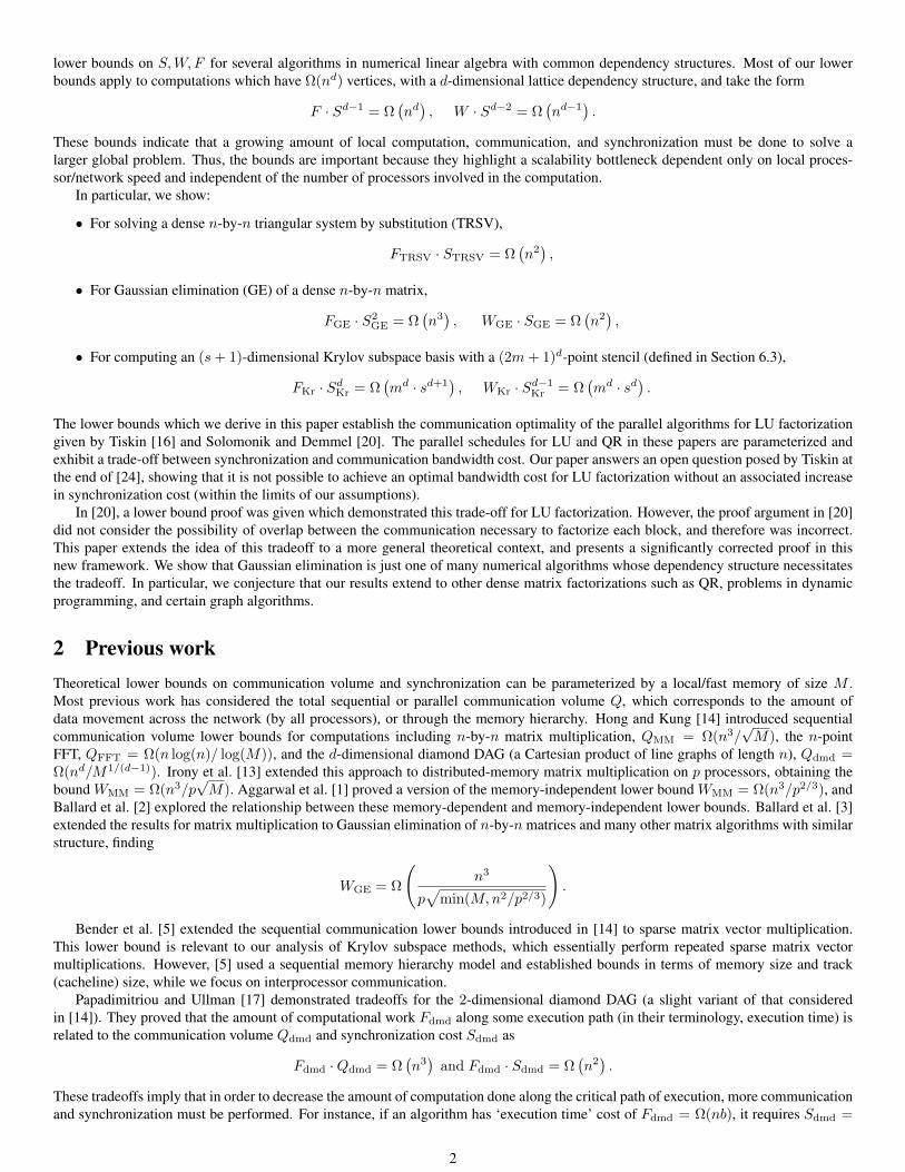
lower bounds on S,W,F for several algorithms in numerical linear algebra with common dependency structures. Most of our lowerbounds apply to computations which have Ω(nd) vertices, with a d-dimensional lattice dependency structure, and take the form

F · Sd−1 = Ω(nd), W · Sd−2 = Ω

(nd−1

).

These bounds indicate that a growing amount of local computation, communication, and synchronization must be done to solve alarger global problem. Thus, the bounds are important because they highlight a scalability bottleneck dependent only on local proces-sor/network speed and independent of the number of processors involved in the computation.

In particular, we show:

• For solving a dense n-by-n triangular system by substitution (TRSV),

FTRSV · STRSV = Ω(n2),

• For Gaussian elimination (GE) of a dense n-by-n matrix,

FGE · S2GE = Ω

(n3), WGE · SGE = Ω

(n2),

• For computing an (s+ 1)-dimensional Krylov subspace basis with a (2m+ 1)d-point stencil (defined in Section 6.3),

FKr · SdKr = Ω(md · sd+1

), WKr · Sd−1

Kr = Ω(md · sd

).

The lower bounds which we derive in this paper establish the communication optimality of the parallel algorithms for LU factorizationgiven by Tiskin [16] and Solomonik and Demmel [20]. The parallel schedules for LU and QR in these papers are parameterized andexhibit a trade-off between synchronization and communication bandwidth cost. Our paper answers an open question posed by Tiskin atthe end of [24], showing that it is not possible to achieve an optimal bandwidth cost for LU factorization without an associated increasein synchronization cost (within the limits of our assumptions).

In [20], a lower bound proof was given which demonstrated this trade-off for LU factorization. However, the proof argument in [20]did not consider the possibility of overlap between the communication necessary to factorize each block, and therefore was incorrect.This paper extends the idea of this tradeoff to a more general theoretical context, and presents a significantly corrected proof in thisnew framework. We show that Gaussian elimination is just one of many numerical algorithms whose dependency structure necessitatesthe tradeoff. In particular, we conjecture that our results extend to other dense matrix factorizations such as QR, problems in dynamicprogramming, and certain graph algorithms.

2 Previous workTheoretical lower bounds on communication volume and synchronization can be parameterized by a local/fast memory of size M .Most previous work has considered the total sequential or parallel communication volume Q, which corresponds to the amount ofdata movement across the network (by all processors), or through the memory hierarchy. Hong and Kung [14] introduced sequentialcommunication volume lower bounds for computations including n-by-n matrix multiplication, QMM = Ω(n3/

√M), the n-point

FFT, QFFT = Ω(n log(n)/ log(M)), and the d-dimensional diamond DAG (a Cartesian product of line graphs of length n), Qdmd =Ω(nd/M1/(d−1)). Irony et al. [13] extended this approach to distributed-memory matrix multiplication on p processors, obtaining thebound WMM = Ω(n3/p

√M). Aggarwal et al. [1] proved a version of the memory-independent lower bound WMM = Ω(n3/p2/3), and

Ballard et al. [2] explored the relationship between these memory-dependent and memory-independent lower bounds. Ballard et al. [3]extended the results for matrix multiplication to Gaussian elimination of n-by-n matrices and many other matrix algorithms with similarstructure, finding

WGE = Ω

(n3

p√

min(M,n2/p2/3)

).

Bender et al. [5] extended the sequential communication lower bounds introduced in [14] to sparse matrix vector multiplication.This lower bound is relevant to our analysis of Krylov subspace methods, which essentially perform repeated sparse matrix vectormultiplications. However, [5] used a sequential memory hierarchy model and established bounds in terms of memory size and track(cacheline) size, while we focus on interprocessor communication.

Papadimitriou and Ullman [17] demonstrated tradeoffs for the 2-dimensional diamond DAG (a slight variant of that consideredin [14]). They proved that the amount of computational work Fdmd along some execution path (in their terminology, execution time) isrelated to the communication volume Qdmd and synchronization cost Sdmd as

Fdmd ·Qdmd = Ω(n3)

and Fdmd · Sdmd = Ω(n2).

These tradeoffs imply that in order to decrease the amount of computation done along the critical path of execution, more communicationand synchronization must be performed. For instance, if an algorithm has ‘execution time’ cost of Fdmd = Ω(nb), it requires Sdmd =

2

Ω(n/b) synchronizations and a communication volume of Qdmd = Ω(n2/b). The tradeoff on Fdmd · Sdmd is a special case of thed-dimensional bubble latency lower bound tradeoff we derive in the next section, with d = 2. This diamond DAG tradeoff was alsodemonstrated by Tiskin [22].

Bampis et al. [4] considered finding the optimal schedule (and number of processors) for computing d-dimensional grid graphs,similar in structure to those we consider in Section 6. Their work was motivated by [17] and took into account dependency graphstructure and communication, modeling the cost of sending a word between processors as equal to the cost of a computation.

We will introduce lower bounds that relate synchronization to computation and data movement along dependency paths. Our workis most similar to the approach in [17]; however, we attain bounds on W (the parallel communication volume along some dependencypath), rather than Q (the total communication volume). Our theory obtains tradeoff lower bounds for a more general set of dependencygraphs which allows us to develop lower bounds for a wider set of computations.

3 Theoretical modelWe first introduce of the mathematical notation we will employ throughout this and later sections

• Sets are defined as uppercase letters (S, V ).

• Vectors are defined as lowercase boldface letters (v) and the ith element of v is indexed as vi.

• Accordingly, matrices and tensors are defined as uppercase boldface letters (A,T), with elements Aij , Tijk.

• Functions and maps will be defined as Greek letters (σ(n)).

• Open/closed intervals in R are denoted (a, b) and [a, b].

The dependency graph of a program is a directed acyclic graph (DAG) G = (V,E). The vertices V = I ∪ Z ∪ O correspond toeither input values I (the vertices with in-degree 0), or the results of (distinct) operations, in which case they are either temporary (orintermediate) values Z, or outputs O. There is an edge (u, v) ∈ E ⊂ V × (Z ∪ O) for each operand u of each operation v. Theseedges represent data dependencies, and impose limits on the parallelism available within the computation. For instance, if G = (V,E)is a line graph with V = v1, . . . , vn and E = (v1, v2), . . . , (vn−1, vn), the computation is entirely sequential, and a lower boundon the execution time is the time it takes a single processor to compute F = n − 1 operations. Using graph expansion and hypergraphanalysis, we will derive lower bounds for computation and communication for dependency graphs with certain properties. Then we willshow that these lower bounds can be applied to several important problems in numerical linear algebra. These lower bounds have theform of tradeoffs between data transfer and synchronization cost and between work and synchronization cost, and form a conceptualcommunication wall which limits parallelism.

A parallelization of an algorithm corresponds to a coloring of its dependency graph, i.e., a partition of the vertices into p disjointsets V =

⋃pi=1 Ci, where processor i for i ∈ 1, . . . , p computes Ci ∩ (Z ∪ O). We require that in any parallel execution among p

processors, at least two processors compute b|Z ∪ O|/pc elements; this assumption is necessary to avoid the case of a single processorcomputing the whole problem sequentially (without parallel communication). Any vertex v of color i (v ∈ Ci) must be communicatedto a different processor j if there is an edge from v to a vertex in Cj (though there need not necessarily be a message going directlybetween processor i and j, as the data can move through intermediate processors). We define each processor’s communicated set as

Ti = u : (u,w) ∈ [(Ci × (V \ Ci)) ∪ ((V \ Ci)× Ci)] ∩ E .

We note that each Ti is a vertex separator in G between Ci \ Ti and V \ (Ci ∪ Ti). For each processor i, a communication schedule,mi, Rij, Fij, Mij, defines a sequence of mi time-steps. The time-steps may differ from processor to processor and relate toeach other only via explicit communication in the schedule. At time-step j ∈ 1, . . . ,mi, processor i receives a set of values Rij ⊂ V(which are packed in one message and originate from a single processor), performs a computation (or no computation) Fij ⊂ V ,|Fij | ≤ 1, and sends a set of values Mij ⊂ V (which are also packed in one message and have a single destination processor). If bothRij andMij are empty, no communication or synchronization is done by processor i at time-step j. Similarly, if Fij = ∅, no computationis done by processor i at time-step j. We require that communication is point-to-point, so each message Mij must be received on someunique processor k at some time-step l, that is Rkl = Mij . The schedule must perform all computations Ci =

⋃mi

j=1 Fij and themessages sent and received by each processor i must include their communicated set Ti ⊂

⋃mi

j=1Mij ∪ Rij (a processor may send andreceive values not in its communicated set in order to avoid synchronization of other processors). Further, the schedule should respectdependencies, that is, for each f ∈ Fij and each (u, f) ∈ E, if u ∈ Ci then u ∈ Fik for some k ∈ 1, . . . , j − 1, and if u /∈ Ci, werequire that u ∈ Rik for some k ∈ 1, . . . , j. Any value sent, ∀u ∈ Mij , must either be an input (u ∈ Ci ∩ I) or must have beenpreviously received or computed by that process, which means there exists k ∈ 1, . . . , j such that u ∈ Fik or u ∈ Rik.

An execution of a parallel algorithm is associated with a communication schedule which can be represented by the weighted DAGG = (V , E). For each processor i ∈ 1, . . . , p and time-step j ∈ 1, . . . ,mi, we include vertex (i, j) ∈ V . The graph includes0-weighted edges ((i, k), (i, k + 1), 0) ∈ E for k ∈ 1, . . . ,mi − 1 (corresponding to sequentially executed computations Fik andFi,k+1). The graph also includes unit-weighted edges, ((i, j), (k, l), 1) ∈ E, for each nonempty message pair, ∅ 6= Mij = Rkl, wherei, k ∈ 1, . . . , p, i 6= k, j ∈ 1, . . . ,mi, l ∈ 1, . . . ,mk.

3

We measure the execution costs by considering all execution paths Π that exist in the communication schedule DAG G: eachexecution path π ∈ Π is of the form π = (i1, j1), . . . , (in, jn) where for each k ∈ 1, . . . , n − 1, ((ik, jk), (ik+1, jk+1), w) ∈ Eand w ∈ 0, 1. Since any two computations on π happen either on the same processor or follow a series of messages, the time toexecute a path is a lower bound on the total execution time. The computation cost corresponds to the longest unweighted path throughthe schedule, i.e.,

F = maxπ∈Π

∑(i,j)∈π

|Fij |.

Note that this value is greater than or equal to the work done by any single processor, i.e., for all i, F ≥∑j |Fij | = |Ci|. The bandwidth

cost of the communication schedule corresponds to the maximum vertex-weighted path through the schedule, with each vertex weightedby the size of the messages Mij and Rij , i.e.,

W = maxπ∈Π

∑(i,j)∈π

|Mij |+ |Rij |.

Similarly, the bandwidth cost is at least as large as that incurred by any single processor, i.e., for all i, W ≥∑j |Mij | + |Rij |.

Accordingly, the latency cost corresponds to the longest edge-weighted path through the schedule. Defining the edge-to-weight mappingω(u, v) = w for each (u, v, w) ∈ E, the maximum weighted path in the schedule is given by

S = max(i1,j1),...,(in,jn)∈Π

n−1∑k=1

ω ((ik, jk), (ik+1, jk+1)) .

Our goal will be to lower bound the bandwidth and latency costs for any parallelization and communication schedule of a given depen-dency graph.

4 General lower bound theorem via bubble expansionIn this section, we introduce the concept of dependency bubbles and their expansion. Bubbles represent sets of interdependent compu-tations, and their expansion allows us to analyze the cost of computation and communication for any parallelization and communicationschedule. We will show that if a dependency graph has a path along which bubbles expand as some function of the length of the path,any parallelization of this dependency graph must sacrifice synchronization or incur higher computational and data volume costs, whichscale with the total size and cross-section size (minimum cut size) of the bubbles, respectively.

4.1 Bubble expansionGiven a dependency graph G = (V,E), we say vn ∈ V depends on v1 ∈ V if and only if there is a path P ⊂ V connecting v1 tovn, i.e., P = v1, . . . , vn such that (v1, v2), . . . , (vn−1, vn) ⊂ E. We denote a sequence of (not necessarily adjacent) verticesw1, . . . , wn a dependency path, if for i ∈ 1, . . . , n− 1, wi+1 is dependent on wi.

The (dependency) bubble around a dependency path P connecting v1 to vn is a sub-DAG β(G,P) = (Vβ , Eβ) where Vβ ⊂ V ,each vertex u ∈ Vβ lies on a dependency path v1, . . . , u, . . . , vn in G, and Eβ = (Vβ × Vβ) ∩ E. This bubble corresponds to allvertices which must be computed between the start and end of the path. Equivalently, the bubble may be defined as the union of all pathsbetween v1 and vn.

4.2 Lower bounds based on bubble expansionA 1

q -balanced vertex separator Q ⊂ V of a graph G = (V,E) splits V \ Q = V1 ∪ V2 so that min(|V1|, |V2|) ≥ b|V |/qc andE ⊂ (V1 × V1) ∪ (V2 × V2) ∪ (Q × V ) ∪ (V × Q). We denote the minimum size |Q| of a 1

q -balanced separator Q of G as χq(G). Ifβ(G,P) is the dependency bubble formed around path P , we say χq(β(G,P)) is its cross-section expansion.

Definition 4.1 We call a directed-acyclic graph G a (ε, σ)-path-expander if there exists a dependency path P in the graph Gand a positive integer constant k |P| such that every subpath R ⊂ P of length |R| ≥ k has bubble β(G,R) = (Vβ , Eβ) withcross-section expansion χq(β(G,R)) = Ω(ε(|R|)) for any real constant q |P|, q > 2, and bubble size |Vβ | = Θ(σ(|R|)), forsome real-valued functions ε, σ which for real numbers b ≥ k are positive and increasing with 1 ≤ ε(b + 1) − ε(b) ≤ cεε(b) and1 ≤ σ(b+ 1)− σ(b) ≤ cσσ(b) for some positive real constants cε, cσ |P|.

Theorem 4.1 (General bubble lower bounds). Suppose a dependency graph G is a (ε, σ)-path-expander about dependency path P .Then, for any parallelization ofG in which no processor computes more than half of the vertices of β(G,P), and for any communicationschedule, there exists an integer b ∈ [k, |P|] such that the computation (F ), bandwidth (W ), and latency (S) costs incurred are

F = Ω (σ(b) · |P|/b) , W = Ω (ε(b) · |P|/b) , S = Ω (|P|/b) .

4

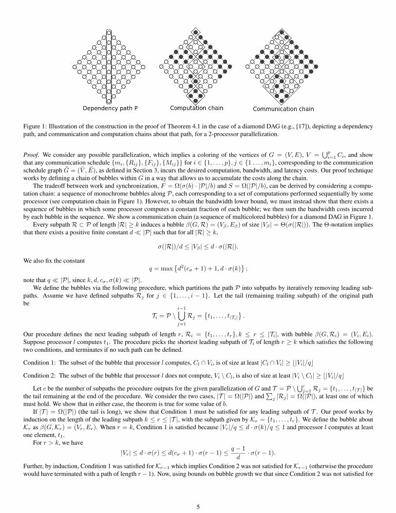
Figure 1: Illustration of the construction in the proof of Theorem 4.1 in the case of a diamond DAG (e.g., [17]), depicting a dependencypath, and communication and computation chains about that path, for a 2-processor parallelization.

Proof. We consider any possible parallelization, which implies a coloring of the vertices of G = (V,E), V =⋃pi=1 Ci, and show

that any communication schedule mi, Rij, Fij, Mij for i ∈ 1, . . . , p, j ∈ 1 . . . ,mi, corresponding to the communicationschedule graph G = (V , E), as defined in Section 3, incurs the desired computation, bandwidth, and latency costs. Our proof techniqueworks by defining a chain of bubbles within G in a way that allows us to accumulate the costs along the chain.

The tradeoff between work and synchronization, F = Ω(σ(b) · |P|/b) and S = Ω(|P|/b), can be derived by considering a compu-tation chain: a sequence of monochrome bubbles along P , each corresponding to a set of computations performed sequentially by someprocessor (see computation chain in Figure 1). However, to obtain the bandwidth lower bound, we must instead show that there exists asequence of bubbles in which some processor computes a constant fraction of each bubble; we then sum the bandwidth costs incurredby each bubble in the sequence. We show a communication chain (a sequence of multicolored bubbles) for a diamond DAG in Figure 1.

Every subpath R ⊂ P of length |R| ≥ k induces a bubble β(G,R) = (Vβ , Eβ) of size |Vβ | = Θ(σ(|R|)). The Θ-notation impliesthat there exists a positive finite constant d |P| such that for all |R| ≥ k,

σ(|R|)/d ≤ |Vβ | ≤ d · σ(|R|).

We also fix the constantq = max

d2(cσ + 1) + 1, d · σ(k)

;

note that q |P|, since k, d, cσ, σ(k) |P|.We define the bubbles via the following procedure, which partitions the path P into subpaths by iteratively removing leading sub-

paths. Assume we have defined subpaths Rj for j ∈ 1, . . . , i − 1. Let the tail (remaining trailing subpath) of the original pathbe

Ti = P \i−1⋃j=1

Rj =t1, . . . , t|Ti|

.

Our procedure defines the next leading subpath of length r, Ri = t1, . . . , tr, k ≤ r ≤ |Ti|, with bubble β(G,Ri) = (Vi, Ei).Suppose processor l computes t1. The procedure picks the shortest leading subpath of Ti of length r ≥ k which satisfies the followingtwo conditions, and terminates if no such path can be defined.

Condition 1: The subset of the bubble that processor l computes, Cl ∩ Vi, is of size at least |Cl ∩ Vi| ≥ b|Vi|/qc

Condition 2: The subset of the bubble that processor l does not compute, Vi \ Cl, is also of size at least |Vi \ Cl| ≥ b|Vi|/qc

Let c be the number of subpaths the procedure outputs for the given parallelization of G and T = P \⋃cj=1Rj = t1, . . . , t|T | be

the tail remaining at the end of the procedure. We consider the two cases, |T | = Ω(|P|) and∑j |Rj | = Ω(|P|), at least one of which

must hold. We show that in either case, the theorem is true for some value of b.If |T | = Ω(|P|) (the tail is long), we show that Condition 1 must be satisfied for any leading subpath of T . Our proof works by

induction on the length of the leading subpath k ≤ r ≤ |T |, with the subpath given by Kr = t1, . . . , tr. We define the bubble aboutKr as β(G,Kr) = (Vr, Er). When r = k, Condition 1 is satisfied because |Vr|/q ≤ d · σ(k)/q ≤ 1 and processor l computes at leastone element, t1.

For r > k, we have

|Vr| ≤ d · σ(r) ≤ d(cσ + 1) · σ(r − 1) ≤ q − 1

d· σ(r − 1).

Further, by induction, Condition 1 was satisfied forKr−1 which implies Condition 2 was not satisfied forKr−1 (otherwise the procedurewould have terminated with a path of length r− 1). Now, using bounds on bubble growth we that since Condition 2 was not satisfied for

5

Kr−1, Condition 1 has to be satisfied for the subsequent bubble, Kr,

|Cl ∩ Vr| ≥ |Cl ∩ Vr−1| ≥ |Vr−1| −⌊|Vr−1|q

⌋≥ q − 1

q|Vr−1| ≥

q − 1

dqσ(r − 1) ≥ 1

q|Vr| ≥

⌊|Vr|q

⌋,

so Condition 1 holds for Kr for r ∈ k, . . . , |T |. Further, since the tail is long, |T | = Ω(|P|), due to Condition 1, processor l mustcompute

F ≥⌊|Vβ(G,T )|/q

⌋= Ω(σ(|T |))

vertices. Since, by assumption, no processor can compute more than half of the vertices of β(G,P), we claim there exists a subpath Qof P , T ⊂ Q ⊂ P , where processor l computes

⌊|Vβ(G,Q)|/q

⌋vertices and does not compute

⌊|Vβ(G,Q)|/q

⌋vertices. The path Q may

always be found to satisfy these two conditions simultaneously, since we can grow Q backward from T until Condition 2 is satisfied,i.e., processor l does not compute at least b|Vβ(G,Q)|/qc vertices, and we will not violate the first condition that (|Cl ∩ Vβ(G,Q)| ≥b|Vβ(G,Q)|/qc, which holds for T , due to bounds on growth of |Vβ(G,Q)|. The proof of this assertion is the same as the inductive proofabove which showed that Condition 1 holds onKr. So, processor l must incur a communication cost proportional to a 1

q -balanced vertexseparator of β(G,Q) with sizeW = Ω(ε(|Q|)) = Ω(ε(|T |)). Since these costs are incurred along a path in the schedule consisting of thework and communication done only by processor l, the bounds hold for b = |T | (note that Ω(|P|/|T |) = Ω(1), because |T | = Ω(|P|)).

In the second case,∑j |Rj | = Ω(|P|), the procedure generates subpaths with a total size proportional to the size of P . For each

i ∈ 1, . . . , c, consider the time-step m during which processor l computed the first vertex t1 on the pathRi, that is, (l,m) ∈ V wherel ∈ 1, . . . , p and m ∈ 1 . . .ml, such that Flm = t1 (recall that each process computes at most one vertex every time-step). Wechoose the smallest s ≥ m such that Cl ∩ Vi ⊂

⋃sm′=m Flm′ (processor l computes its part of Vi between time-steps m and s). Now

consider the time-step v on processor u, (u, v) ∈ V , during which the last vertex tr on the path Rj was computed, that is, (u, v) ∈ Vwhere u ∈ 1, . . . , p and v ∈ 1, . . . ,mu, such that Fuv = tr. Note that for some z ∈ Vi, Fls = z, (otherwise, s can betaken to be to s − 1, and so is not the smallest) and tr is dependent on z (tr is dependent on all vertices in the bubble). So, therewill be an execution path πi = (l,m), . . . , (l, s), . . . , (u, v) ⊂ V in the communication schedule. This path has outgoing messagesMlm, . . . ,Mls, . . . ,Muv and incoming messages Rlm, . . . , Rls, . . . , Ruv that include all vertices in Vi which processor l mustcommunicate to compute Vi ∩ Cl, which is given by the set

Til = u : (u,w) ∈ [(Cl × (Vi \ Cl)) ∪ ((Vi \ Cl)× Cl)] ∩ Ei ,

which is a separator of β(G,Ri) and is 1q -balanced due to Conditions 1 and 2 in the definition of Ri. We use the lower bound on the

minimum separator of a bubble to obtain a lower bound on the size of the communicated set for processor l in the ith bubble,

|Til| ≥ χq(β(G,Ri)) = Ω (ε(|Ri|)) ,

where we are able to bound the growth of β(G,Ri), since |Ri| ≥ k. There exists a dependency path between the last element ofRi andthe first ofRi+1 since they are subpaths of P , so every bubble β(G,Ri) must be computed entirely before any members of β(G,Ri+1)are computed. Therefore, there is an execution path πcritical ⊂ V in the communication schedule which contains πi ⊂ πcritical as a subpathfor every i ∈ 1, . . . , c. Communication and computation along πcritical can be bounded below by

F =∑

(i,j)∈πcritical

|Fij | ≥c∑i=1

1

q|β(G,Ri)| = Ω

(c∑i=1

σ(|Ri|)

),

W=∑

(i,j)∈πcritical

|Mij |+ |Rij | ≥c∑i=1

χq(β(G,Ri))= Ω

(c∑i=1

ε(|Ri|)

).

Further, since each bubble contains vertices computed by multiple processes, between the first and last vertex on the subpath formingeach bubble, a network latency cost of at least one must be incurred per bubble, therefore,

S ≥= Ω(c).

Because σ(b+ 1)−σ(b) ≥ 1 for b ≥ k ≥ |Ri|, and the sum of all the lengths of the subpaths is bounded (∑i |Ri| ≤ |P|), the above

lower bounds for F and W are minimized when allRi are of the same length1. Picking this length as b, that is |Ri| = b = Θ(|P|/c) forall i, leads to a simplified form for the bounds,

F = Ω (σ(b) · |P|/b) , W = Ω (ε(b) · |P|/b) , S = Ω (|P|/b) .

1This mathematical relation can be demonstrated by a basic application of Lagrange multipliers.

6

Corollary 4.2 (d-dimensional bubble lower bounds). Let P be a dependency path in G, such that every subpath R ⊂ P of length|R| ≥ k, where k |P|, has bubble β(G,R) = (Vβ , Eβ) with cross-section expansion χq(β(G,R)) = Ω(|R|d−1) for any constant2 ≤ q |P| and bubble size |Vβ | = Θ(|R|d), for an integer 2 ≤ d k. The computation, bandwidth, and latency costs incurredby any parallelization of G in which no processor computes more than half of the vertices of β(G,P), and with any communicationschedule, must obey the relations

F · Sd−1 = Ω(|P|d

), W · Sd−2 = Ω

(|P|d−1

).

Proof. This is an application of Theorem 4.1 with ε(b) = bd−1 and σ(b) = bd. The theorem yields

F = Ω(bd−1 · |P|

), W = Ω

(bd−2 · |P|

), S = Ω (|P|/b) .

These equations can be manipulated algebraically to obtain

F · Sd−1 = Ω(|P|d

), W · Sd−2 = Ω

(|P|d−1

).

5 Lower bounds on lattice hypergraph cutsFor any hypergraph H = (V,E), we say a hyperedge e ∈ E is internal to some V ′ ⊂ V if e ⊂ V ′. If no e ∈ E is adjacent to (i.e.,contains) a v ∈ V ′ ⊂ V , then say V ′ is disconnected from H . A 1

q -balanced (hyperedge) cut of is a subset of E whose removal fromH partitions V = V1 ∪ V2 with min(|V1|, |V2|) ≥ 1

q |V | such that all remaining (uncut) hyperedges are internal to one of the two parts.We define a d-dimensional lattice hypergraph H = (V,E) of breadth n, with |V | =

(nd

)vertices and |E| =

(nd−1

)hyperedges.

Each vertex is represented as vi1,...,id = (i1, . . . , id) for i1, . . . , id ∈ 1, . . . , nd with i1 < · · · < id. Each hyperedge connects allvertices which share d − 1 indices, that is ej1,...,jd−1

for j1, . . . , jd−1 ∈ 1, . . . , nd−1 with j1 < · · · < jd−1 includes all verticesvi1,...,id for which j1, . . . , jd−1 ⊂ i1, . . . , id. There are n−(d−1) vertices per hyperedge, and each vertex appears in d hyperedges.Each hyperedge intersects (d− 1)(n− (d− 1)) other hyperedges, each at a unique vertex.

A key step in the lower bound proofs in [13] and [3] was the use of an inequality introduced by Loomis and Whitney [15]. We willuse this inequality (in the following form) to prove a lower bound on the cut size of a lattice hypergraph.

Theorem 5.1 (Loomis-Whitney). Let V be a set of d-tuples (i1, . . . , id) ∈ Nd, and consider projections πj : Nd → Nd−1 for j ∈1, . . . , d defined as

πj(i1, . . . , id) = (i1, . . . , ij−1, ij+1, . . . , id),

then the cardinality of V is bounded by,

|V | ≤d∏j=1

|πj(V )|1/(d−1).

Theorem 5.2. For 2 ≤ d, q n, the minimum 1q -balanced cut of a d-dimensional lattice hypergraph H = (V,E) is of size εq(H) =

Ω(nd−1/q(d−1)/d).

Proof. We prove Theorem 5.2 by induction on the dimension, d. In the base case d = 2, we must show that εq(H) = Ω(n/√q).

Consider any 1q -balanced cut Q ⊂ E, which splits the vertices into two disjoint sets V1 and V2. Note that in 2 dimensions, every pair of

hyperedges overlaps, i.e., for i1, i2 ∈ 1, . . . , n with i1 < i2, ei1 ∩ ei2 = vi1,i2. If the first partition, V1, has an internal hyperedge,then since every pair of hyperedges overlaps, V1 is adjacent to all hyperedges inH . Therefore, every hyperedge adjacent to the other partV2 ⊂ V must be in the cut, Q. On the other hand, if V1 has no internal hyperedges, then all hyperedges adjacent to V1 must connect bothparts, and thus are cut. So, without loss of generality we will assume that V2 is disconnected after the cut. We now argue that Ω(n/

√q)

hyperedges must be cut to disconnect V2.Since the cut is 1

q -balanced, we know that |V2| ≥ n(n− 1)/(2q). To disconnect each vi1,i2 ∈ V2, both adjacent hyperedges (ei1 andei2 ) must be cut. We can bound from below the cut size by first obtaining a lower bound on the product of the sizes of the projectionsπ1(vi1,i2) = i2 and π2(vi1,i2) = i1 via the Loomis-Whitney inequality (Theorem 5.1),

|π1(V2)| · |π2(V2)| ≥ |V2| ≥ n(n− 1)/(2q),

and then concluding

εq(H) = |π1(V2) ∪ π2(V2)|

εq(H) ≥ 1

2(|π1(V2)|+ |π2(V2)|)

≥√|π1(V2)| · |π2(V2)| ≥

√n(n− 1)/(2q)

= Ω (n/√q) ,

7

since the size of the union of the two projections equals the number of hyperedges that must be cut to disconnect V2.For the inductive step, we assume that the theorem holds for dimension d − 1 and prove that it must also hold for dimension d,

where d ≥ 3. In d dimensions, we define a hyperplane xk1,...,kd−2for each k1, . . . , kd−2 ∈ 1, . . . , nd−2 with k1 < · · · < kd−2

as the set of all hyperedges ej1,...,jd−1which satisfy k1, . . . , kd−2 ⊂ j1, . . . , jd−1. Thus, each of the |X| =

(nd−2

)hyperplanes

contains n− (d−2) hyperedges, and each hyperedge is in d−1 hyperplanes. Note that each hyperplane shares a unique hyperedge with(d−2)(n− (d−2)) other hyperplanes. Further, each hyperedge in a hyperplane intersects each other hyperedge in the same hyperplanein a unique vertex, and the set of all these vertices are precisely those sharing the d− 2 indices defining the hyperplane.

Consider any 1q -balanced hypergraph edge cut Q ⊂ E. Since all hyperedges which contain vertices in both V1 and V2 must be part

of the cut Q, all vertices are either disconnected completely by the cut or remain in hyperedges which are all internal to either V1 or V2.Let U1 ⊂ V1 be the vertices contained in a hyperedge internal to V1 and let U2 ⊂ V2 be the vertices contained in a hyperedge internal toV2. Since both V1 and V2 contain bnd/qc vertices, either bnd/2qc vertices must be in internal hyperedges within both V1 as well as V2,that is,

case (i): |U1| ≥ bnd/2qc and |U2| ≥ bnd/2qc,

or there must be bnd/2qc vertices that are disconnected completely by the cut,

case (ii): |(V1 \ U1) ∪ (V2 \ U2)| ≥ bnd/2qc.

In case (i), since both U1 and U2 have at least bnd/2qc vertices, we know that there are at least |U1|/(n − (d − 1)) ≥ bnd−1/2qchypergraph edges W1 which are internal to V1 after the cut Q, and a similar set of hyperedges W2 internal to V2. We now obtain a lowerbound on the size of the cut Q for this case by counting the hyperplanes which Q must contain. Our argument relies on the idea that iftwo hypergraph edges are in the same hyperplane, the entire hyperplane must be disconnected (all of its hyperedges must be part of thecut Q) in order to disconnect the two edges. This allows us to bound the number of hyperplanes which must be disconnected in orderfor W1 to be disconnected from W2.

We define a new (d − 1)-dimensional lattice hypergraph H ′ = (E,X), with vertices and hyperedges equal to the hyperedges andhyperplanes of the original hypergraph H . The cut Q induces a 1

2q -balanced cut on H ′ since it creates two disconnected partitions ofhyperedges: W1 and W2, each of size bnd−1/2qc. We can assert a lower bound on the size of any 1

2q -balanced cut of H ′ by induction,

εq(H′) = Ω

(nd−2/(2q)

(d−2)/(d−1))

= Ω(nd−2/q(d−2)/(d−1)

).

This lower bound on cut size of H ′ yields a lower bound on the number of hyperplanes which must be cut to disconnect the hyperedgesinto two balanced sets W1 and W2. Remembering that disconnecting each hyperplane requires cutting all of its internal n − (d − 2)hyperedges (and also that each pair of hyperplanes overlap on at most one hyperedge), allows us to conclude that the number ofhyperedges cut (in Q) must be at least

εq(H) ≥ (n− (d− 2))

d− 1εq(H

′) = Ω(nd−1/q(d−2)/(d−1)

).

The quantity on the right is always larger than the lower bound we are trying to prove, εq(H) = Ω(nd−1/q(d−1)/d), so the proof for thiscase is complete.

In case (ii), we know that bnd/2qc vertices U ⊂ V are disconnected by the cut (before the cut, every vertex was adjacent to dhyperedges). We define d projections,

πj(vi1,...,id) = (i1, . . . , ij−1, ij+1, . . . , id)

for j ∈ 1, . . . , d corresponding to each of d hyperedges adjacent to vi1...id . We apply the Loomis-Whitney inequality (Theorem 5.1)to obtain a lower bound on the product of the size of the projections,

d∏j=1

|πj(U)|1/(d−1) ≥ |U | ≥ bnd/2qc,

and then conclude with a lower bound on the number of hyperedges in the cut of H ,

εq(H) ≥ |d⋃j=1

πj(U)| ≥ 1

d

d∑j=1

|πj(U)| ≥ 1

d

d∏j=1

|πj(U)|1/d

= Ω((nd/2q

)(d−1)/d)

= Ω(nd−1/q(d−1)/d

),

where we discard the constant 1d by applying our assumption that d n. By induction, this lower bound holds for all 2 ≤ d n.

8

6 ApplicationsIn this section, we apply the general theorems derived in the previous sections to obtain lower bounds on the costs associated with a fewspecific numerical linear algebra algorithms. We treat the dependency graphs of the algorithms in a general manner by reducing them tolattice hypergraphs.

Consider a dependency graph G = (V,E) and a partition Ei of its edge set E. Let Vi be all the vertices adjacent to the edgepartition Ei for each i (while Ei is a disjoint partition of E, Vi is not necessarily a disjoint partition of V ). We can define ahypergraph H = (V,D) based on G, where in each hyperedge di ∈ D, every pair of vertices u, v ∈ di is connected in G via a pathconsisting of edges in Ei. By defining H in this manner, any cut of C ⊂ E corresponds to a hypergraph cut of H with at most |C|hyperedges, which may be obtained by cutting all hyperedges di ∈ D corresponding to parts Ei which contain cut edges, i.e., ∃e ∈ Eisuch that e ∈ C.

We will also employ hyperedges to obtain lower bounds on sets of vertices connected via arbitrary reduction (sum) trees. Anyreduction tree T = (R,E) which sums a set of vertices S ⊂ R must connect each pair of vertices in S. Therefore, we can define ahypergraph edge corresponding to this reduction tree, which contains the edges in S (ignoring the intermediate vertices R \ S whichdepend on the particular tree), with the edge partition corresponding to the hyperedge being E for any possible reduction tree T =(R,E).

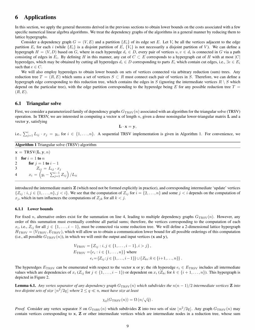
6.1 Triangular solveFirst, we consider a parameterized family of dependency graphsGTRSV(n) associated with an algorithm for the triangular solve (TRSV)operation. In TRSV, we are interested in computing a vector x of length n, given a dense nonsingular lower-triangular matrix L and avector y, satisfying

L · x = y,

i.e.,∑ij=1 Lij · xj = yi, for i ∈ 1, . . . , n. A sequential TRSV implementation is given in Algorithm 1. For convenience, we

Algorithm 1 Triangular solve (TRSV) algorithm

x = TRSV(L,y, n)

1 for i = 1 to n2 for j = 1 to i− 13 Zij = Lij · xj4 xi =

(yi −

∑i−1j=1 Zij

)/Lii

introduced the intermediate matrix Z (which need not be formed explicitly in practice), and corresponding intermediate ‘update’ verticesZij : i, j ∈ 1, . . . , n, j < i. We see that the computation of Zij for i = 2, . . . , n and some j < i depends on the computation ofxj , which in turn influences the computations of Zjk for all k < j.

6.1.1 Lower bounds

For fixed n, alternative orders exist for the summation on line 4, leading to multiple dependency graphs GTRSV(n). However, anyorder of this summation must eventually combine all partial sums; therefore, the vertices corresponding to the computation of eachxi, i.e., Zij for all j ∈ 1, . . . , i − 1, must be connected via some reduction tree. We will define a 2-dimensional lattice hypergraphHTRSV = (VTRSV, ETRSV), which will allow us to obtain a communication lower bound for all possible orderings of this computation(i.e., all possible GTRSV(n)), in which we will omit the output and input vertices (x and y),

VTRSV = Zij : i, j ∈ 1, . . . , i− 1, i > j ,ETRSV =ei : i ∈ 1, . . . , n where

ei=Zij :j ∈ 1,. . ., i−1∪Zki :k ∈ i+1,. . ., n .

The hyperedges ETRSV can be enumerated with respect to the vector x or y; the ith hyperedge ei ∈ ETRSV includes all intermediatevalues which are dependencies of xi (Zij for j ∈ 1, . . . , i − 1) or dependent on xi (Zki for k ∈ i + 1, . . . , n). This hypergraph isdepicted in Figure 2.

Lemma 6.1. Any vertex separator of any dependency graph GTRSV(n) which subdivides the n(n − 1)/2 intermediate vertices Z intotwo disjoint sets of size bn2/2qc where 2 ≤ q n, must have size at least

χq(GTRSV(n)) = Ω (n/√q) .

Proof. Consider any vertex separator S on GTSRV(n) which subdivides Z into two sets of size bn2/2qc. Any graph GTRSV(n) maycontain vertices corresponding to x, Z or other intermediate vertices which are intermediate nodes in a reduction tree, whose sum

9

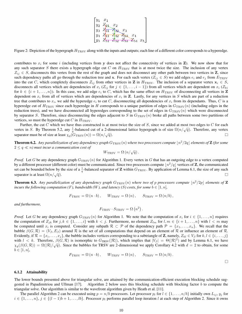
Figure 2: Depiction of the hypergraphHTRSV along with the inputs and outputs; each line of a different color corresponds to a hyperedge.

contributes to xi for some i (including vertices from y does not affect the connectivity of vertices in Z). We now show that forany such separator S there exists a hypergraph edge cut C on HTRSV that is at most twice the size. The inclusion of any vertexZij ∈ S, disconnects this vertex from the rest of the graph and does not disconnect any other path between two vertices in Z, sincesuch dependency paths all go through the reduction tree and x. For each such vertex (Zij ∈ S) we add edges ei and ej from ETRSV

into the cut C, which completely disconnects Zij from other vertices in Z in HTRSV. The inclusion of a separator vertex xi ∈ S,disconnects all vertices which are dependencies of xi (Zij for j ∈ 1, . . . , i − 1) from all vertices which are dependent on xi (Zkifor k ∈ i + 1, . . . , n). In this case, we add edge ei to C, which has the same effect on HTRSV of disconnecting all vertices in Zdependent on xi from all of vertices which are dependencies of xi in Z. Lastly, for any vertices in S which are part of a reductiontree that contributes to xi, we add the hyperedge ei to cut C, disconnecting all dependencies of xi from its dependants. Thus, C is ahyperedge cut of HTRSV since each hyperedge in H corresponds to a unique partition of edges in GTRSV(n) (including edges in thereduction trees), and we have disconnected all hyperedges corresponding to the set of edges in GTRSV(n) which were disconnectedby separator S. Therefore, since disconnecting the edges adjacent to S in GTRSV(n) broke all paths between some two partitions ofvertices, so must the hyperedge cut C in HTRSV.

Further, the cut C which we have thus constructed is at most twice the size of S, since we added at most two edges to C for eachvertex in S. By Theorem 5.2, any 1

q -balanced cut of a 2-dimensional lattice hypergraph is of size Ω(n/√q). Therefore, any vertex

separator must be of size at least χq(GTRSV(n)) = Ω(n/√q).

Theorem 6.2. Any parallelization of any dependency graphGTRSV(n) where two processors compute bn2/2qc elements of Z (for some2 ≤ q n) must incur a communication cost of

WTRSV = Ω (n/√q) .

Proof. Let G be any dependency graph GTRSV(n) for Algorithm 1. Every vertex in G that has an outgoing edge to a vertex computedby a different processor (different color) must be communicated. Since two processors compute bn2/qc vertices of Z, the communicatedset can be bounded below by the size of a 1

q -balanced separator of Z within GTRSV. By application of Lemma 6.1, the size of any suchseparator is at least Ω(n/

√q).

Theorem 6.3. Any parallelization of any dependency graph GTRSV(n) where two of p processors compute bn2/2pc elements of Zincurs the following computation (F ), bandwidth (W ), and latency (S) costs, for some b ∈ [1, n],

FTRSV = Ω (n · b) , WTRSV = Ω (n) , STRSV = Ω (n/b) ,

and furthermore,FTRSV · STRSV = Ω

(n2).

Proof. Let G be any dependency graph GTRSV(n) for Algorithm 1. We note that the computation of xi for i ∈ 1, . . . , n requiresthe computation of Zjk for j, k ∈ 1, . . . , i with k < j. Furthermore, no element Zlm for l,m ∈ i + 1, . . . , n with l < m maybe computed until xi is computed. Consider any subpath R ⊂ P of the dependency path P = x1, . . . , xn. We recall that thebubble β(G,R) = (Vβ , Eβ) around R is the set of all computations that depend on an element of R or influence an element of R.Evidently, ifR = xi, . . . , xj, the bubble includes vertices corresponding to a subtriangle of Z, namely, Zkl ∈ Vβ for k, l ∈ i, . . . , jwith l < k. Therefore, β(G,R) is isomorphic to GTRSV(|R|), which implies that |Vβ | = Θ(|R|2) and by Lemma 6.1, we haveχq(β(G,R)) = Ω(|R|/√q). Since the bubbles for TRSV are 2-dimensional we apply Corollary 4.2 with d = 2 to obtain, for someb ∈ [1, n],

FTRSV = Ω (n · b) , WTRSV = Ω (n) , STRSV = Ω (n/b) .

6.1.2 Attainability

The lower bounds presented above for triangular solve, are attained by the communication-efficient execution blocking schedule sug-gested in Papadimitriou and Ullman [17]. Algorithm 2 below uses this blocking schedule with blocking factor b to compute thetriangular solve. Our algorithm is similar to the wavefront algorithm given by Heath et al. [11].

The parallel Algorithm 2 can be executed using p = n/b processors. Let processor pl for l ∈ 1, . . . , n/b initially own Lij , yj fori ∈ 1, . . . , n, j ∈ (l − 1)b + 1, . . . , lb. Processor pl performs parallel loop iteration l at each step of Algorithm 2. Since it owns

10

Algorithm 2 Parallel triangular solve (TRSV) algorithm

x = TRSV(L,y, n)

1 x = y2 for k = 1 to n/b3 // Each processor pl executes a unique iteration of below loop4 parallel for l = max(1, 2k − n/b) to k5 if l > 16 Receive length b vector x[(2k − l − 1)b+ 1 : (2k − l)b] from processor pl−1

7 for i = (2k − l − 1)b+ 1 to (2k − l)b8 for j = (l − 1)b+ 1 to min(i− 1, lb)9 xi = (xi − Lij · xj)

10 if k = l11 xi = xi/Lii12 if l < n/b13 Send length b vector x[(2k − l − 1)b+ 1 : (2k − l)b] to processor pl+1

14 parallel for l = max(1, 2k + 1− n/b) to k15 if l > 116 Receive length b vector x[(2k − l)b+ 1 : (2k − l + 1)b] from processor pl−1

17 for i = (2k − l)b+ 1 to (2k − l + 1)b18 for j = (l − 1)b+ 1 to lb19 xi = (xi − Lij · xj)20 if l < n/b21 Send length b vector x[(2k − l)b+ 1 : (2k − l + 1)b] to processor pl+1

the necessary panel of L and vector part xj , no communication is required outside the vector send/receive calls listed in the code. So ateach iteration of the outer loop at least one processor performs O(b2) work, and 2b data is sent, requiring 2 messages. Therefore, thisalgorithm achieves the following costs,

FTRSV = O(nb), WTRSV = O(n), STRSV = O(n/b),

which attains our communication lower bounds in Theorems 6.2 and 6.3 for any b ∈ 1, n. Parallel TRSV algorithms in current numer-ical libraries such as Elemental [18] and ScaLAPACK [6] employ algorithms that attain our lower bound, modulo an extra O(log(p))factor on the latency cost, due to their use of collectives for communication rather than the point-to-point communication in our wave-front TRSV algorithm.

6.2 Gaussian eliminationIn this section, we show that the Gaussian elimination algorithm has 3-dimensional bubble-growth and dependency graphs which satisfythe path expansion properties necessary for the application of Corollary 4.2 with d = 3. We consider factorization of a symmetricmatrix via Cholesky, as well as Gaussian elimination of a dense nonsymmetric matrix. We show that these factorizations of n-by-nmatrices form an intermediate 3D tensor Z such that Zijk ∈ Z for i > j > k ∈ 1, . . . , n and Zijk is dependent on each Zlmnfor l > m > n ∈ 1, . . . j − 1. We assume that a fast matrix multiplication algorithm is not used, though we conjecture that ouranalysis can be extended to account for potential use of Strassen’s matrix multiplication algorithm and likely other fast algorithms formultiplication.

6.2.1 Cholesky factorization

The Cholesky factorization of a symmetric positive definite matrix A is

A = L · LT ,

for a lower-triangular matrix L. A simple sequential algorithm for Cholesky factorization is given in Algorithm 3. We introduced anintermediate tensor Z, whose elements must be computed during any execution of the Cholesky algorithm (although Z itself need not bestored explicitly in an actual implementation). We note that the Floyd-Warshall [10, 25] all-pairs shortest-path graph algorithm has thesame dependency structure as Cholesky for undirected graphs (and Gaussian Elimination for directed graphs), so our lower bounds maybe easily extended to this case. However, interestingly our lower bounds for this graph algorithm are not valid for the all-pairs shortest-paths problem in general, which may alternatively be solved via path-doubling (a technique which naively incurs an extra computationalcost, but may be augmented to have the same asymptotic costs as matrix multiplication, as shown by Tiskin [23]).

11

Algorithm 3 Cholesky factorization algorithm

L = CHOLESKY(A, n)

1 for j = 1 to n

2 Ljj =√Aij −

∑j−1k=1 Ljk · Ljk

3 for i = j + 1 to n4 for k = 1 to j − 15 Zijk = Lik · Ljk6 Lij = (Aij −

∑j−1k=1 Zijk)/Ljj

6.2.2 LU factorization

The LU factorization of a square matrix A isA = L ·U,

for a lower-triangular matrix L and a unit-diagonal upper triangular matrix U (we make U rather than L have a unit-diagonal fornotational convenience). A simple non-pivoted algorithm for LU factorization is given in Algorithm 4. Within the computation of

Algorithm 4 LU factorization algorithm

L,U = LU(A, n)

1 for j = 1 to n2 for i = 1 to j − 13 for k = 1 to i− 14 Zjik = Lik · Ukj5 Uij = Aij −

∑i−1k=1 Zjik

6 Ljj = Aij −∑j−1k=1 Ljk · Ukj

7 for i = j + 1 to n8 for k = 1 to j9 Zijk = Lik · Ukj

10 Lij = (Aij −∑j−1k=1 Zijk)/Ljj

LU factorization, the n3/6 intermediate vertices in Z within Algorithm 4 are analogous to the intermediate vertices of the Choleskycomputation of the previous section. The vertices designated as Z in the LU computation are ignored in our further analysis. Ignoringvertices does not invalidate our lower bounds because they can only necessitate more work and communication.

6.2.3 Lower bounds

We note that the summations on lines 2 and 6 of Algorithm 3 as well as lines 6 and 10 of Algorithm 4 can be computed via anysummation order (and will be computed in different orders in different parallel algorithms). This implies that the summed verticesare connected in any dependency graph GGE(n), but the connectivity structure may be different. We define a 3-dimensional latticehypergraph HGE = (VGE, EGE) for the algorithm which allows us to obtain a lower bound for any possible summation order, as

VGE =Zijk : i, j, k ∈ 1, . . . , n, i > j > k,EGE =ei,j : i, j ∈ 1, . . . , n with i > j where

ei,j = Zijk : k ∈ 1, . . . , j − 1 ∪ Zikj : k ∈ j + 1, . . . , i− 1 ∪ Zkij : k ∈ i+ 1, . . . , n

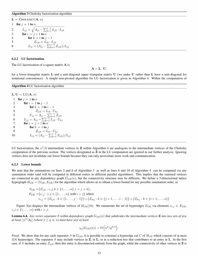
Figure 3(a) displays the intermediate vertices of HGE(16). We enumerate the set of hyperedges EGE via elements ei,j ∈ EGE,i, j ∈ 1, . . . , n with i > j.

Lemma 6.4. Any vertex separator S within dependency graph GGE(n) that subdivides the intermediate vertices Z into two sets of sizeat least bn3/3qc (where 2 ≤ q n) must have size at least

χq(GGE(n)) = Ω(n2/q2/3

).

Proof. We show that for any such separator S in GGE, it is possible to construct a hyperedge cut C of HGE which consists of at most3|S| hyperedges. The separator S may include vertices in Z, in L, or in a reduction tree that contributes to an entry in L. In the firstcase, if S includes an entry Zijk, then this entry is disconnected entirely from the graph, while the connectivity of other vertices in Z is

12

(a) (b)

Figure 3: These diagrams show (a) the vertices Zijk in VGE with n = 16 and (b) the hyperplane x12 and hyperedge e12,6 on HGE.

not affected. For each such entry Zijk ∈ S we add edges ei,j , ei,k and ej,k to C, effectively disconnecting Zijk within the hypergraphHGE. In the latter two cases, if S includes entry Lij or an entry to a reduction tree that contributes to Lij , we add edge ei,j to C.Including the entry Lij or a intermediate in a reduction tree which contributes to it disconnects vertices which are dependent on Lijfrom the dependencies thereof. These dependencies are encoded in the hypergraph HGE by the edge ei,j , the removal of which servesto break all possible paths that could have gone through Lij or the reduction tree in HGE. Now we ascertain that C is a hyperedge cutof HGE since each hyperedge in H corresponds to a unique partition of edges in GGE(n) (including edges in the reduction trees), andwe have disconnected all hyperedges corresponding to the set of edges in GGE(n) which were disconnected by separator S. Therefore,since disconnecting the edges adjacent to S broke all paths between some two partitions of vertices in GGE(n), the hyperedge cut Cmust disconnect the same partitions in HGE.

For each vertex in S, we have added at most 3 edges to the hyperedge cut C, and have disconnected the same or larger sets of verticeswithin the hypergraph in each case. By Theorem 5.2, a 1

q -balanced cut of the vertices Z in HGE is of size Ω(n2/q2/3). Therefore, anyvertex separator on a GGE(n) must be of size at least χq(GGE(n)) = Ω(n2/q2/3).

Theorem 6.5. Any parallelization of any dependency graphGGE(n), where two processors each compute bn3/3qc elements of Z (VGE),must incur a communication of

WGE = Ω(n2/q2/3

).

Proof. For any GGE(n), every vertex that has an outgoing edge to a vertex computed by a different processor (different color) must becommunicated. Since two processors each compute bn3/3qc elements of Z, the communicated set can be bounded below by the size ofa 1q -balanced separator of the vertices Z in GGE(n). By Lemma 6.4, the size of any such separator is Ω(n2/q2/3).

Theorem 6.6. Any parallelization of any dependency graphGGE(n) in which two of p processors compute bn3/3pc vertices of Z incursthe following computation (F ), bandwidth (W ), and latency (S) costs, for some b ∈ [1, n],

FGE = Ω(n · b2

), WGE = Ω (n · b) , SGE = Ω (n/b) ,

and furthermore,FGE · S2

GE = Ω(n3), WGE · SGE = Ω

(n2).

Proof. Let G be a dependency graph of GGE(n). We note that the computation of Lii for i ∈ 1, . . . , n requires the computationof Zlmk for l,m, k ∈ 1, . . . , i with l > m > k. Furthermore, no element Zsrt for s, r, t ∈ i + 1, . . . , n with s > r > tcan be computed until Lii is computed. Consider any subpath R ⊂ P of the dependency path P = L11, . . . , Lnn. Evidently, ifR = Lii, . . . , Lj+1,j+1, the bubble β(G,R) = (Vβ , Eβ) includes vertices corresponding to a subcube of Z, namely Zklm ∈ Vβ fork, l,m ∈ i, . . . , j with k > l > m. Therefore, β(G,R) is isomorphic to GGE(|R|), which implies that |Vβ | = Θ(|R|3) and byLemma 6.4, we have χq(β(G,R)) = Θ(|R|2/q2/3). Since we have 3-dimensional bubbles with 2-dimensional cross-sections, we applyCorollary 4.2 with d = 3 to obtain, for some b ∈ [1, n],

FGE = Ω(n · b2

), WGE = Ω (n · b) , SGE = Ω (n/b) .

13

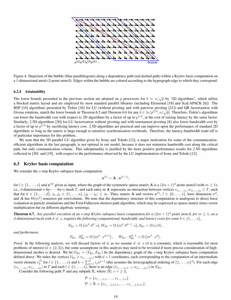
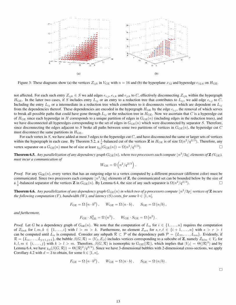
Figure 4: Depiction of the bubble (blue parallelogram) along a dependency path (red dashed path) within a Krylov basis computation ona 1-dimensional mesh (2-point stencil). Edges within the bubble are colored according to the hypergraph edge to which they correspond.

6.2.4 Attainability

The lower bounds presented in the previous section are attained on p processors for b ≈ n/√p by ‘2D algorithms’, which utilize

a blocked matrix layout and are employed by most standard parallel libraries (including Elemental [18] and ScaLAPACK [6]). TheBSP [16] algorithms presented by Tiskin [16] for LU (without pivoting and with pairwise pivoting [21]) and QR factorization withGivens rotations, match the lower bounds in Theorem 6.5 and Theorem 6.6 for any b ∈ [n/p2/3, n/

√p]. Therefore, Tiskin’s algorithms

can lower the bandwidth cost with respect to 2D algorithms by a factor of up to p1/6, at the cost of raising latency by the same factor.Similarly, 2.5D algorithms [20] for LU factorization without pivoting and with tournament pivoting [8] also lower bandwidth cost bya factor of up to p1/6 by sacrificing latency cost. 2.5D algorithms are practical and can improve upon the performance of standard 2Dalgorithms so long as the matrix is large enough to amortize synchronization overheads. Therefore, the latency-bandwidth trade-off isof particular importance for this problem.

We note that the 3D parallel LU algorithm given by Irony and Toledo [12], a major motivation for some of the communication-efficient algorithms in the last paragraph, is not optimal in our model, because it does not minimize bandwidth cost along the criticalpath, but only communication volume. This suboptimality is justified by the more positive performance results for 2.5D algorithmscollected in [20] and [19], with respect to the performance observed by the LU implementation of Irony and Toledo [12].

6.3 Krylov basis computationWe consider the s-step Krylov subspace basis computation

x(l) = A · x(l−1),

for l ∈ 1, . . . , s and x(0) given as input, where the graph of the symmetric sparse matrix A is a (2m+ 1)d-point stencil (with m ≥ 1),i.e., d-dimensional n-by-· · · -by-n mesh T , and each entry in A represents an interaction between vertices vi1,...,id , wj1,...,jd ∈ T , suchthat for k ∈ 1, . . . , d, ik, jk ∈ 1, . . . , n, |jk − ik| ≤ m. Thus, matrix A and vectors x(l), l ∈ 0, . . . , s, have dimension nd,and A has Θ(md) nonzeros per row/column. We note that the dependency structure of this computation is analogous to direct forceevaluation in particle simulations and the Ford-Fulkerson shortest-path algorithm, which may be expressed as sparse-matrix times vectormultiplication but on different algebraic semirings.

Theorem 6.7. Any parallel execution of an s-step Krylov subspace basis computation for a (2m + 1)d-point stencil, for m ≥ 1, on ad-dimensional mesh with d s, requires the following computational, bandwidth, and latency costs for some b ∈ 1, . . . s,

FKr = Ω(md·bd·s

),WKr = Ω

(md·bd−1·s

), SKr = Ω (s/b) .

and furthermore,FKr · SdKr = Ω

(md · sd+1

), WKr · Sd−1

Kr = Ω(md · sd

).

Proof. In the following analysis, we will discard factors of d, as we assume d s (d is a constant), which is reasonable for mostproblems of interest (d ∈ 2, 3), but some assumptions in this analysis may need to be revisited if more precise consideration of high-dimensional meshes is desired. We let GKr = (VKr, EKr) be the dependency graph of the s-step Krylov subspace basis computationdefined above. We index the vertices VKr 3 vi1,...,id,l with d+ 1 coordinates, each corresponding to the computation of an intermediatevector element x(l)

k for l ∈ 1, . . . , s and k =∑dj=1 ijn

j−1 (this assumes the lexicographical ordering of 1, . . . , nd). For each edge(vi1,...,id , wj1,...,jd) in T and each l ∈ 1, . . . , s, there is an edge (vi1,...,id,l−1, wj1,...,jd,l) in EKr.

Consider the following path P and any subpathR, where |R| = r ≥ 3,

P = v1,...,1,1, . . . , v1,...,1,sP ⊃ R = v1,...,1,h+1, . . . , v1,...,1,h+r .

14

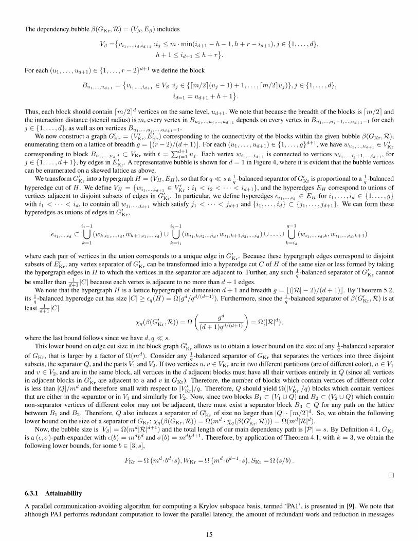
The dependency bubble β(GKr,R) = (Vβ , Eβ) includes

Vβ =vi1,...,id,id+1

:ij ≤ m ·min(id+1 − h− 1, h+ r − id+1), j ∈ 1, . . . , d,h+ 1 ≤ id+1 ≤ h+ r

.

For each (u1, . . . , ud+1) ∈ 1, . . . , r − 2d+1 we define the block

Bu1,...,ud+1=vi1,...,id+1

∈ Vβ :ij ∈ dm/2e(uj − 1) + 1, . . . , dm/2euj), j ∈ 1, . . . , d,id=1 = ud+1 + h+ 1

.

Thus, each block should contain dm/2ed vertices on the same level, ud+1. We note that because the breadth of the blocks is dm/2e andthe interaction distance (stencil radius) is m, every vertex in Bu1,...,uj ,...,ud+1

depends on every vertex in Bu1,...,uj−1,...,ud+1−1 for eachj ∈ 1, . . . , d, as well as on vertices Bu1,...,uj ,...,ud+1−1.

We now construct a graph G′Kr = (V ′Kr, E′Kr) corresponding to the connectivity of the blocks within the given bubble β(GKr,R),

enumerating them on a lattice of breadth g = b(r− 2)/(d+ 1)c. For each (u1, . . . , ud+1) ∈ 1, . . . , gd+1, we have wu1,...,ud+1∈ V ′Kr

corresponding to block Bu1,...,ud,t ⊂ VKr with t =∑d+1j=1 uj . Each vertex wi1,...,id+1

is connected to vertices wi1,...,ij+1,...,id+1, for

j ∈ 1, . . . , d+ 1, by edges in E′Kr. A representative bubble is shown for d = 1 in Figure 4, where it is evident that the bubble verticescan be enumerated on a skewed lattice as above.

We transformG′Kr into a hypergraphH = (VH , EH), so that for q s a 1q -balanced separator ofG′Kr is proportional to a 1

q -balancedhyperedge cut of H . We define VH = wi1,...,id+1

∈ V ′Kr : i1 < i2 < · · · < id+1, and the hyperedges EH correspond to unions ofvertices adjacent to disjoint subsets of edges in G′Kr. In particular, we define hyperedges ei1,...,id ∈ EH for i1, . . . , id ∈ 1, . . . , gwith i1 < · · · < id, to contain all wj1,...,jd+1

which satisfy j1 < · · · < jd+1 and i1, . . . , id ⊂ j1, . . . , jd+1. We can form thesehyperedges as unions of edges in G′Kr,

ei1,...,id ⊂i1−1⋃k=1

(wk,i1,...,id , wk+1,i1,...,id) ∪i2−1⋃k=i1

(wi1,k,i2...,id , wi1,k+1,i2,...,id) ∪ . . . ∪g−1⋃k=id

(wi1,...,id,k, wi1,...,id,k+1)

where each pair of vertices in the union corresponds to a unique edge in G′Kr. Because these hypergraph edges correspond to disjointsubsets of E′Kr, any vertex separator of G′Kr can be transformed into a hyperedge cut C of H of the same size or less formed by takingthe hypergraph edges in H to which the vertices in the separator are adjacent to. Further, any such 1

q -balanced separator of G′Kr cannotbe smaller than 1

d+1 |C| because each vertex is adjacent to no more than d+ 1 edges.We note that the hypergraph H is a lattice hypergraph of dimension d + 1 and breadth g = b(|R| − 2)/(d + 1)c. By Theorem 5.2,

its 1q -balanced hyperedge cut has size |C| ≥ εq(H) = Ω(gd/qd/(d+1)). Furthermore, since the 1

q -balanced separator of β(G′Kr,R) is atleast 1

d+1 |C|

χq(β(G′Kr,R)) = Ω

(gd

(d+ 1)qd/(d+1)

)= Ω(|R|d),

where the last bound follows since we have d, q s.This lower bound on edge cut size in the block graph G′Kr allows us to obtain a lower bound on the size of any 1

q -balanced separatorof GKr, that is larger by a factor of Ω(md). Consider any 1

q -balanced separator of GKr that separates the vertices into three disjointsubsets, the separatorQ, and the parts V1 and V2. If two vertices u, v ∈ VKr are in two different partitions (are of different color), u ∈ V1

and v ∈ V2, and are in the same block, all vertices in the d adjacent blocks must have all their vertices entirely in Q (since all verticesin adjacent blocks in G′Kr are adjacent to u and v in GKr). Therefore, the number of blocks which contain vertices of different coloris less than |Q|/md and therefore small with respect to |V ′Kr|/q. Therefore, Q should yield Ω(|V ′Kr|/q) blocks which contain verticesthat are either in the separator or in V1 and similarly for V2. Now, since two blocks B1 ⊂ (V1 ∪Q) and B2 ⊂ (V2 ∪Q) which containnon-separator vertices of different color may not be adjacent, there must exist a separator block B3 ⊂ Q for any path on the latticebetween B1 and B2. Therefore, Q also induces a separator of G′Kr of size no larger than |Q| · dm/2ed. So, we obtain the followinglower bound on the size of a separator of GKr: χq(β(GKr,R)) = Ω(md · χq(β(G′Kr,R))) = Ω(md|R|d).

Now, the bubble size is |Vβ | = Ω(md|R|d+1) and the total length of our main dependency path is |P| = s. By Definition 4.1, GKr

is a (ε, σ)-path-expander with ε(b) = mdbd and σ(b) = mdbd+1. Therefore, by application of Theorem 4.1, with k = 3, we obtain thefollowing lower bounds, for some b ∈ [3, s],

FKr = Ω(md·bd·s

),WKr = Ω

(md·bd−1·s

), SKr = Ω (s/b) .

6.3.1 Attainability

A parallel communication-avoiding algorithm for computing a Krylov subspace basis, termed ‘PA1’, is presented in [9]. We note thatalthough PA1 performs redundant computation to lower the parallel latency, the amount of redundant work and reduction in messages

15

made possible by redundant work are not asymptotically significant, and thus the lower bounds of Theorem 6.7 apply. Computing ans-step Krylov subspace basis with a (2m + 1)d-point stencil with block size b ∈ 1, . . . s can be accomplished by s/b invocations ofPA1 with basis size parameter b. The costs for the overall computation using PA1 are then

FKr =s

b·O(bd+1md) = O(md · bd · s),

WKr =s

b·O(bdmd) = O(md · bd−1 · s),

SKr =s

b·O(1) = O(s/b),

under the assumption n/p1/d = O(bm). This algorithm therefore attains the lower bounds and lower bound tradeoffs of Theorem 6.7.

7 ConclusionOur lower bounds showed that many numerical problems which have lattice dependency structure, require execution costs which areindependent of the number of processors but dependent on the problem size. Architecturally, our results provided lower bounds onexecution time, as a function of synchronization latency (α), communication throughput (β), and clock-speed (γ). The tradeoffs wederive describe the strong scaling limit of Gaussian Elimination and Krylov basis computation in terms of these three quantities. In otherwords, we obtained bounds on the time it takes for any number of processors to solve a system of linear equations via certain numericalalgorithms based on the network and clock speed of each processor. An interesting piece of future work will be to consider Krylov basiscomputations, which are analogous to the Ford-Fulkerson single-source shortest-paths graph algorithm, on graphs such as expanders andbinary trees rather than just stencils (grids), which our graph-based bubble-expansion formulation should allow.

8 AcknowledgementsWe would like to thank Satish Rao, Grey Ballard, and Benjamin Lipshitz for particularly useful discussions on topics encompassed withinthis paper. The first author was supported by a Krell Department of Energy Computational Science Graduate Fellowship, grant numberDE-FG02-97ER25308. We also acknowledge the support of the US DOE (grants DE-SC0003959, DE-SC0004938, DE-SC0005136,DE-SC0008700, DE-AC02-05CH11231) and DARPA (award HR0011-12-2-0016).

References[1] A. Aggarwal, A.K. Chandra, and M. Snir. Communication complexity of PRAMs. Theoretical Computer Science, 71(1):3 – 28,

1990.

[2] G. Ballard, J. Demmel, O. Holtz, B. Lipshitz, and O. Schwartz. Strong scaling of matrix multiplication algorithms and memory-independent communication lower bounds (brief announcement). In ACM Symposium on Parallelism in Algorithms and Architec-tures (SPAA), June 2012.

[3] G. Ballard, J. Demmel, O. Holtz, and O. Schwartz. Minimizing communication in linear algebra. SIAM J. Mat. Anal. Appl., 32(3),2011.

[4] E. Bampis, C. Delorme, and J.-C. Konig. Optimal schedules for d-D grid graphs with communication delays. In STACS 96, volume1046 of Lecture Notes in Computer Science, pages 655–666. Springer Berlin Heidelberg, 1996.

[5] M. A. Bender, G. S. Brodal, R. Fagerberg, R. Jacob, and E. Vicari. Optimal sparse matrix dense vector multiplication in theI/O-model. Theory of Computing Systems, 47(4):934–962, 2010.

[6] L. S. Blackford, J. Choi, A. Cleary, E. D’Azeuedo, J. Demmel, I. Dhillon, S. Hammarling, G. Henry, A. Petitet, K. Stanley,D. Walker, and R. C. Whaley. ScaLAPACK user’s guide. Society for Industrial and Applied Mathematics, Philadelphia, PA, USA,1997.

[7] D. Culler, R. Karp, D. Patterson, A. Sahay, K. E. Schauser, E. Santos, R. Subramonian, and T. von Eicken. LogP: towards arealistic model of parallel computation. In Proceedings of the fourth ACM SIGPLAN symposium on Principles and practice ofparallel programming, PPOPP ’93, pages 1–12, New York, NY, USA, 1993. ACM.

[8] J. Demmel, L. Grigori, and H. Xiang. A Communication Optimal LU Factorization Algorithm. EECS Technical Report EECS-2010-29, UC Berkeley, March 2010.

[9] J. Demmel, M. Hoemmen, M. Mohiyuddin, and K. Yelick. Avoiding communication in computing Krylov subspaces. TechnicalReport UCB/EECS-2007-123, EECS Dept., U.C. Berkeley, Oct 2007.

16

[10] R.W. Floyd. Algorithm 97: Shortest path. Commun. ACM, 5:345, June 1962.

[11] M.T. Heath and C.H. Romine. Parallel solution of triangular systems on distributed-memory multiprocessors. SIAM Journal onScientific and Statistical Computing, 9(3):558–588, 1988.

[12] D. Irony and S. Toledo. Trading replication for communication in parallel distributed-memory dense solvers. Parallel ProcessingLetters, 71:3–28, 2002.

[13] D. Irony, S. Toledo, and A. Tiskin. Communication lower bounds for distributed-memory matrix multiplication. Journal of Paralleland Distributed Computing, 64(9):1017 – 1026, 2004.

[14] H. Jia-Wei and H. T. Kung. I/O complexity: The red-blue pebble game. In Proceedings of the thirteenth annual ACM symposiumon Theory of computing, STOC ’81, pages 326–333, New York, NY, USA, 1981. ACM.

[15] L.H. Loomis and H. Whitney. An inequality related to the isoperimetric inequality. Bulletin of the AMS, 55:961–962, 1949.

[16] W. F. McColl and A. Tiskin. Memory-efficient matrix multiplication in the BSP model. Algorithmica, 24:287–297, 1999.

[17] C. Papadimitriou and J. Ullman. A communication-time tradeoff. SIAM Journal on Computing, 16(4):639–646, 1987.

[18] J. Poulson, B. Maker, J. R. Hammond, N. A. Romero, and R. van de Geijn. Elemental: A new framework for distributed memorydense matrix computations. ACM Transactions on Mathematical Software, 39(2):13, 2013.

[19] E. Solomonik, A. Bhatele, and J. Demmel. Improving communication performance in dense linear algebra via topology awarecollectives. In Supercomputing, Seattle, WA, USA, Nov 2011.

[20] E. Solomonik and J. Demmel. Communication-optimal 2.5D matrix multiplication and LU factorization algorithms. In SpringerLecture Notes in Computer Science, Proceedings of Euro-Par, Bordeaux, France, Aug 2011.

[21] D.C. Sorensen. Analysis of pairwise pivoting in Gaussian Elimination. Computers, IEEE Transactions on, C-34(3):274 –278,March 1985.

[22] A Tiskin. The Design and Analysis of Bulk-Synchronous Parallel Algorithms. PhD thesis, University of Oxford, 1998.

[23] A. Tiskin. All-pairs shortest paths computation in the BSP model. Lecture Notes in Computer Science, Automata, Languages andProgramming, 2076:178–189, 2001.

[24] A. Tiskin. Communication-efficient parallel generic pairwise elimination. Future Generation Computer Systems, 23(2):179 – 188,2007.

[25] S. Warshall. A theorem on boolean matrices. J. ACM, 9:11–12, January 1962.

17