BANCO CENTRAL DE RESERVA DEL PERÚ

Trade linkages and growth in Latin America: A time-varying SVAR approach

Diego Winkelried* y Miguel Angel Saldarriaga*

* Banco Central de Reserva del Perú

DT. N° 2012-011 Serie de Documentos de Trabajo

Working Paper series Abril 2012

Los puntos de vista expresados en este documento de trabajo corresponden a los autores y no reflejan

necesariamente la posición del Banco Central de Reserva del Perú.

The views expressed in this paper are those of the authors and do not reflect necessarily the position of the Central Reserve Bank of Peru.

Trade linkages and growth in Latin America:A time-varying SVAR approach∗†

Diego Winkelried

and

Miguel Angel Saldarriaga

April 19, 2012

Abstract

This paper examines how shocks originated in large economies around the globe have transmittedto the growth rates of Latin American countries. For this purpose, a highly parsimonious structuralVAR model – identified through bilateral trade linkages – is proposed, tested, estimated and simulated.Since trade weights evolve through time, the effect of shocks are time-varying. Thus, we are able toquantify how growth in the region has been affected by tighter trading linkages with fast-growingemerging economies, and how it has responded to a new world trade structure, featuring China as amajor player. It is found that about half of the vigourous growth reported in Latin American countriesby the end of the 2000s can be attributed to (direct and especially indirect) multiplier effects inducedby the spectacular growth of the Chinese economy over the same period.

JEL Classification : C32, C50, E32, F44, O54.Keywords : Latin America, China, trade linkages, time-varying structural VAR.

∗Winkelried: Central Reserve Bank of Peru (email: diego.winkelried@bcrp.gob.pe, diegowq@cantab.net), Saldarriaga: Central ReserveBank of Peru (email: miguel.saldarriaga@bcrp.gob.pe).

†We would like to thank Eduardo Morón, Paul Castillo and seminar participants at the Central Reserve Bank of Peru for helpfulcomments. We are also grateful to Donita Rodriguez for her help in assembling the dataset used in our estimations. All remaining errors areours. The opinions herein are those of the authors and do not necessarily reflect those of the Central Reserve Bank of Peru.

1 Introduction

It has been widely discussed that during the last two decadesa new global context has emerged as the result ofa deeper integration between countries and regions and because of the high growth of emerging countries, whosecontribution to the world growth has been increasing. As reported byIzquierdo and Talvi(2011), the main traits ofthis new global economic order, which became evident after the 2008 financial crisis, are the reallocation of worldoutput and demand from industrial countries to emerging markets, and the redirection of world savings providingabundant and inexpensive international resources to emerging economies.

The reallocation of world output and demand came in tandem with dramatic changes in trade patterns. For LatinAmerican countries, there has been a substantial shift in its trade towards emerging markets. At the beginning ofthe 1990s, the United States was Latin America’s main trade partner, followed by European countries, while theonly Asian country among the top trade partners was Japan. Incontrast, by the end of the last decade, China hasbecome the main trade partner for Brazil, Chile and Peru, andadvanced the ranking in the remaining Latin Americancountries. Also, whereas the United States remains among the top trade partners, many European countries had beendisplaced by Asian or other Latin American economies (see Table 1).

This redirection of trade mirrors a higher degree of business cycle synchronization among emerging economies.Dela Torre(2011) stress that whereas business cycles in Latin America countries and China have become increasinglycorrelated, they seem to have decoupled from the rich countries’ cycles, a process that was particularly notoriouswith the unexpectedly fast recovery after the financial crisis of 2008. Nevertheless, direct trade linkages are not theonly channel through which growth can be affected. As argued byCalderón(2009), indirect linkages, the effectsthrough third countries that are also important trade partners, may be even stronger. Table1 shows that China hasbecome an important destination to Latin American exports as well as to exports of large industrialized economies:the Chinese share of American exports rose from 1.9 percent in 1991 to 9.0 percent in 2010, whereas the share ofGerman exports increased from to 0.9 to 8.2 percent. These figures hint that, in the new world trade configuration,the influence of the Chinese economy on Latin America is likely to be manifested not only by stronger direct tradelinks, but also by indirect effects through its increasing importance for the region’s traditional main trade partners.

The purpose of this paper is to investigate the implicationsof this new global scenario, where emerging markets –particularly China – are more prominent in the world economy, for Latin American growth. In particular, we aim toanswer the following questions:

• How has Latin American growth responded to shocks to traditional trade partners like the United States and,to a lower extent, Germany? Have these responses changed by the emergence of China as a global actor?

• Are the healthy growth rates observed in Latin American during the 2000s a byproduct of the Chinesejuggernaut? If so, were they due to a closer bilateral relationship with China or to second-round effectsof China’s boosting demand?

• Even though the Chinese economy is the most emblematic and sounding case of a large fast-growingemerging economy, the new global order has witnessed the emergence of others as well. For instance, LatinAmerica is celebrating that Brazil has recently overtaken the United Kingdom as the world’s sixth largesteconomy. But, does a shock to the Brazilian economy exert similar effects across the region than a shock toChina? In other words, does a Brazilian shock have global impacts?

In order to answer these questions, followingAbeysinghe and Forbes(2005), we estimate and simulate a structuralVAR (SVAR) model for the growth rates of 29 countries around the globe, for the last two decades. To achieve aparsimonious yet dynamically rich specification, we constrained the feedback effects from a country’s trade partnersto its own growth rates by consider a “rest of the world” aggregate rather that each trade partner individually.Time-varying bilateral trade weights are used in the aggregation, and this enables us to explore how the complexinteractions across the growth rates of the 29 countries in our sample has evolved through time. In particular, theSVAR model capture not only the direct effects of trade, but also indirect effects such that a shock to one countrycan have large effects on others, even if they are minor trading partners.

2

Table 1. Export shares for Latin American (LA) and selected countries, 1991 and 2010

UnitedStates

Germany Brazil China Rest ofEurope

Rest ofLA

Rest ofAsia

Others

1991

Argentina 13.6 8.0 16.3 2.7 31.7 17.4 8.8 1.4Brazil 26.0 8.8 − 0.9 26.3 17.1 17.9 2.9Chile 21.2 9.4 5.9 1.1 25.8 8.5 27.1 1.1Colombia 48.0 9.3 0.9 0.3 18.1 17.4 4.5 1.5Ecuador 62.8 6.2 0.8 0.0 10.9 15.5 2.9 0.9Mexico 83.8 1.3 0.5 0.0 6.1 1.9 3.6 2.9Peru 26.8 6.6 3.9 5.7 23.6 14.4 16.5 2.5Uruguay 11.8 10.1 28.3 7.4 18.2 17.5 5.1 1.6Venezuela 70.7 5.2 2.9 0.0 8.0 6.4 4.2 2.5

LA Average 40.5 7.2 7.4 2.0 18.7 12.9 10.1 1.9

United States − 6.3 1.8 1.9 21.8 13.5 26.7 28.0Germany 9.5 − 0.7 0.9 76.7 1.9 8.2 2.0China 10.0 3.8 0.1 − 6.5 0.5 77.2 1.9

2010

Argentina 7.0 3.5 27.6 11.1 16.4 22.3 8.7 3.3Brazil 13.2 5.5 − 20.9 19.4 25.2 13.7 2.0Chile 11.4 1.5 7.0 28.3 14.6 10.4 23.3 3.6Colombia 50.9 0.8 3.1 5.9 13.9 18.2 5.5 1.7Ecuador 45.9 2.4 0.4 2.5 11.8 31.6 4.6 0.6Mexico 83.1 1.2 1.3 1.5 3.4 3.8 1.8 4.0Peru 15.8 4.4 2.9 18.0 23.9 12.3 10.7 12.0Uruguay 3.7 8.3 25.9 17.2 15.6 23.9 4.4 1.1Venezuela 57.8 1.3 1.0 11.1 4.2 4.2 19.5 1.0

LA Average 32.1 3.2 8.7 12.9 13.7 16.9 10.2 3.3

United States − 4.7 3.5 9.0 15.7 21.2 19.3 26.6Germany 9.2 − 1.7 8.2 68.0 2.5 8.3 2.1China 24.2 5.8 2.1 − 14.9 3.9 44.7 4.5

Notes: The export share for countryi is computed as the ratio of exports from countryi (row) to region or countryj (column), to the sum ofexports from countryi to the 29 countries listed in section3.1. The list is comprehensive but excludes Africa, Central America, the MiddleEast and Eastern Europe. The shares sum to 100 across rows.Source: Direction of Trade Statistics (IMF).

The increase in globalization over the last 20 years has highlighted the importance and pervasiveness of internationallinkages in the world economy, and the importance of capturing those linkages in empirical macroeconomic models.Thus, there is a large literature in international economics exploiting such interrelationships. Early studies includeNorrbin and Schlagenhauf(1996), Elliott and Fatas(1996), and more recentlyAbeysinghe and Forbes(2005),Canova(2005), Enders and Souki(2008) andCanova and Ciccarelli(2009). The most popular thread is related tothe so-called global VAR (GVAR) advanced inPesaran et. al.(2004) and extended inDees et. al.(2007). Recently,Cesa-Bianchi et. al.(2011) have used the GVAR approach to answer questions similar to those formulated above.

Even though our modeling approach is related to the GVAR, there are some important methodological differences.Firstly, our model is smaller as it includes one variable percountry (GDP growth). Even though this preventsus to label shocks more adequately (for instance, supply versus demand shocks), it allows us to formally testthe aggregation hypothesis that is taken for granted in the GVAR literature. Secondly, our identification strategydiffers in that we also use the aggregation restrictions to identify structural country specific shocks. Thirdly, wepropose a standardized impulse response function that can be interpreted as an elasticity, in order to deal with thedifferent variances of shocks across countries in the model. Finally, we exploit the aggregation restrictions further

3

to explore order and rank conditions for instrumental variable estimation. In this way, we do not need to rely onweak exogeneity assumptions, that every single country in the world – but the United States – is treated as a smallopen economy, that are ubiquitous in the traditional GVAR approach.

We find strong evidence that supports the increasing effects of China over Latin America’s growth, in agreementwith Cesa-Bianchi et. al.(2011). We also find weak but indicative evidence of diminishing effects of the UnitedStates and Germany. On the other hand, our results indicate that Brazilian shocks are qualitatively different to theChinese ones, because its second-round effects are only important in a few neighboring countries. The results alsopoint out to indirect effects of China’s growth to explain the accelerating growth ofmost Latin America countries.

The remainder of the paper is organized as follows. Section2 discusses methodological issues and develops anSVAR that allows for rich feedbacks parsimoniously. Furthermore, a formal hypothesis test on the aggregationrestrictions, embedded in the SVAR, is proposed. Section3 describes the data, presents time-varying impulseresponse functions, and analyzes the shifts in the effects of a shock originated in the United States, China, Germanyand Brazil. Counterfactual simulations are also performedto quantify and disentangle the gains for Latin Americancountries of the new trade structure. Section4 gives closing remarks and avenues for further research.

2 Methodological issues

This section discusses the econometric framework used to investigate how the feedbacks amongst the growth ratesof n countries around the globe have evolved in the last two decades. Two major points are considered. Firstly,aggregation restrictions are imposed into a standard, potentially large reduced form VAR of growth rates, and weformally test their significance. These restrictions not only promote parsimony but also identify a structural formand suggest valid and relevant instruments for estimation.Secondly, as inAbeysinghe and Forbes(2005) andCesa-Bianchi et. al.(2011), we allow the bilateral trade weights to evolve through time, thereby capturing rich dynamicsreflected in a changing direction in Latin American trade towards emerging markets. This feature allows us tocompute time-varying impulse response functions.

2.1 The aggregation hypothesis

Our starting point is the reduced form VAR(p) model

yt =

p∑

r=1

Ar yt−r + εt , (1)

whereyt is ann × 1 vector of endogenous variables whosei-th element corresponds to the growth rate of countryi in period t, Ar (r = 1, 2, . . . , p) are coefficient matrices andεt is the vector of mutually correlatediid statisticalinnovations. The covariance matrix ofεt is ann× n positive define matrixΩε.

It is well-documented that the usefulness of a dynamic modellike (1) may be limited in finite samples due tothe proliferation of parameters that need to be estimated. Indeed, each additional lag implies the estimation ofn2

coefficients, and these may be poorly estimated with the sample sizes typically encountered in applications. Thus,promoting parsimony by imposing meaningful restrictions on matricesAr is likely to improve the inferential contentof testing procedures based on the VAR system. This is the purpose of aggregation restrictions, where given weightsare used in the construction of aggregated variables that maintain feedback effects across countries.

Consider an aggregate composed by the (n− 1) variables inyt other thanyi,t,

xi,t =

n∑

j=1

wi j y j,t wheren∑

j=1

wi j = 1 and wii = 0 . (2)

The definition of the aggregatexi,t is general. The weightswi j may be time-varying, but to avoid cluttering thenotation we leave this time dependence implicit (we relax this formulation below). Also, the weightswi j areconstrainednot to be estimated jointly withAr , otherwise the linearity in the VAR model may be lost with

4

aggregation. This situation corresponds to either non-random weights or stochastic weights that are predetermined,i.e. its determination (and so its estimation) is independent from εt.

Take thei-th equation in the unrestricted VAR (1)

yi,t =

p∑

r=1

aii (r)yi,t−r +

p∑

r=1

n∑

j,i

ai j (r)y j,t−r + εi,t , (3)

whereyi,t is thei-th element ofyt, εi,t is the i-th element ofεt, andai j (r) denotes the (i, j)-th element ofAr . In analternative, restricted model all dynamic feedback toyi,t come from its own lags and lags of the aggregate,

yi,t =

p∑

r=1

aii (r)yi,t−r +

p∑

r=1

ci(r)xi,t−r + εi,t =

p∑

r=1

aii (r)yi,t−r +

p∑

r=1

n∑

j,i

ci(r)wi j y j,t−r + εi,t . (4)

If ai j (r) = ci(r)wi j , then the restricted model (4) is equivalent to the model without restrictions (3). Thesep(n− 1)equalities imply a total ofp(n− 1)− p = p(n− 2) restrictions that take the form

ai j (r) −

[

wi j

wik

]

aik(r) = 0 for j , k, k , i and r = 1, 2, . . . , p . (5)

Thus, the aggregation restrictions imply that the non-diagonal elements of thei-th row of Ar are proportional toeach other, and the proportionality factor is given by the ratio wi j/wik. In other words,y j,t andyk,t affect the expectedvalue of future realizations ofyi,t proportionally to their contributions to the aggregate (2).

The unrestricted model is obtained by regressingyi,t on thep lags ofyt. This amounts topncoefficients per equationand pn2 in the entire VAR. On the other hand, in the restricted modelyi,t is regressed on itsp lags and thep lagsof the aggregatexi,t. Here, each equation has 2p coefficients and the restricted VAR has 2pn coefficients. Thus,the aggregation restrictions can reduce the number of coefficients to be estimated substantially, even for moderatevalues ofn. For instance, ifp = 2 andn = 10 then we havepn2

= 200 coefficients in the unrestricted model, andonly 2pn= 40 in the restricted, a total ofnp(n− 2) = 160 restrictions.

The aggregation restrictions can be conveniently reinterpreted as exclusion restrictions, and this is the basis forhypothesis testing. After simple manipulations, the original equation (3) can be rewritten as

yi,t =

p∑

r=1

aii (r)yi,t−r +

p∑

r=1

ci(r)xi,t−r +

p∑

r=1

n∑

j,i

δi j (r)y j,t−r + εi,t , (6)

whereδi j (r) = ai j (r)−ci (r)wi j for r = 1, . . . p, j = 1, 2, . . . , n and j , i. Therefore, the restricted model hasδi j (r) = 0for all r and j , i. Thus, testing the aggregation hypothesis amounts to estimate the extended equation (6) via OLSand testingH0 : δi j (r) = 0 using a standard Wald statistic. Note thatH0 has the appealing interpretation that oncexi,t is controlled for, its constituentsy j,t have no predictive power onyi,t.

2.2 The structural model

Even though the reduced form is used to investigate whether aconstrained model based on aggregation restrictionsserves as a valid characterization of the data, the ultimateobject of interest is a model that allows a contemporaneousfeedback fromxi,t to yi,t. In econometric jargon, we seek a structural form (SVAR) associated to the reduced form(1), after imposing the aggregation restrictions. Thei-th equation of such structural model is

yi,t =

p∑

r=1

φi(r)yi,t−r +

p∑

r=0

βi(r)xi,t−r + ui,t , (7)

where ui,t is a structural shock to thei-th county growth rate. To express the system in matrix form,defineBr = diag(β1(r), β2(r), . . . , βn(r) ) andΦr = diag(φ1(r), φ2(r), . . . , φn(r) ) as then× n diagonal matrices that collect

5

the coefficients associated to ther-th lag effects. Define alsoWt as then× n matrix whose (i, j) element iswi j,t, andrecall thatwii ,t = 0 for all t. Then, upon stacking alln equations of the form (7), we obtain

(In − B0Wt)yt =

p∑

r=1

(Φr + BrWt−r )yt−r + ut . (8)

The consequences of imposing aggregation restrictions canbe clearly appreciated in the SVAR (8), where then× nfeedback matrixΦr + BrWt−r contains only 2n unknown parameters, and then × n matrix of contemporaneouseffectsIn − B0Wt, which is similar to that inElliott and Fatas(1996), contains onlyn free parameters. Therefore,unlike the SVAR tradition where the structural form – especially its contemporaneous effects and the covariancematrix of the structural shocks – needs to be restricted in order to achieve identification, the aggregation restrictionssolely identify the model: whereas the reduced form contains pn2 free parameters, the structural has onlyn(2p+1),so that identification is achieved under the mild condition that p(n − 2) ≥ 1.1 Importantly, identification followsfrom the fact thatWt is predetermined, i.e. its estimation is independent from the estimation of the SVAR.

Another interesting feature of (8) is that it is a time-varying SVAR. As such, it has the flexibility of stabilizing theestimates of the time invariant coefficients (Br andΦr ) in the presence of major shocks, such as international crises.By construction, changes in the historical bilateral tradestructures through time will be reflected in all relationshipsinvolved in the SVAR, either indirect and direct, contemporaneous or lagged. Moreover, sinceWt is likely to evolvesmoothly, so will the coefficients in (8), a result that is usually enforced by letting them follow correlated randomwalks, a favorite specification in time-varying VARs (cf.Primiceri, 2005). Nevertheless, since the changing natureof the model parameters is linked to the evolution of the predetermined weightsWt, the treatment of their stochasticproperties is greatly simplified (see, for instance, section 2.4).

2.3 Impulse response analysis

The time-varying nature of the coefficient matrices in (8) imply that functions of these matrices, such as the impulseresponse function, also depend ont. This is an interesting property of the model and allows us toinvestigate howdifferent configurations of theWt matrices (different trade structures) affect the dynamic responses of the system.

Conditional on a particular trade configurationWt = W for all t, the SVAR becomes time invariant and can begiven the moving average representation

yt = Θ0ut +Θ1ut−1 +Θ2ut−2 +Θ3ut−3 + . . . . (9)

The matricesΘh satisfy the recursion

Θh = C1Θh−1 + C2Θh−2 + · · · + CpΘh−p , (10)

with Θ0 = C0 andΘh = 0 for h < 0 as initial conditions, andC0 = (In − B0W)−1 andCr = C0(Φr + BrW) (thedependence onW is left implicit to alleviate the notation). The responses to a structural shock afterh periods aregiven by the elements ofΘh. The accumulated responses are collected inΨh = Θ0 +Θ1 + . . . +Θh.

Following Winkelried (2011), to compare the effects of shocks of different sizes amongst countries, we entertaina standardized response that takes into account the relative variability of the different shocks inut. Let ei be an× 1 selection vector with unity as itsi-th element and zeros elsewhere. Suppose we perturb thei-th element ofut

(u0 = ei), a shock that is interpreted as a structural perturbation to thei-th country’s growth rate. Therelative effectof shock i on country j after h periodsis given by

ρi j (h) =ej′Ψhei

ei′Ψhei

. (11)

After h periods, the structural shock has an accumulated effect ofei′Ψhei on thei-th country’s growth rate. Thus,

given the linearity of (9), settingu0 = ei/(ei′Ψhei) renders a shock that produces an increase in thei-th growth rate

1 This count does not include the parameters in the covariancematrices of the innovationsεt and structural shocksut. In both cases, theseare unconstrained parameters so the above order condition is not altered.

6

of exactly one percent afterh periods. The definition of (11) is simply the cumulative response of the growth rate ofcountry j to such a shock, i.e. how much of the shock to thei-th perturbation passes through thej-th growth rate.

The relative effects summarize complicated dynamics in the SVAR. The impacteffectsρi j (0) can be regarded asa direct responseto the shock, transmitted immediately, and depends heavilyon the bilateral relationship betweencountriesi and j, in particular on the weightw ji . On the other hand, further effectsρi j (h) for h > 0 include theinfluence of the shock being propagated to other economies inthe system. Thus, forh > 0 the relative effects areindirect multipliers. Due to these multipliers, a shock to one country can have large effects on others even if theyare minor trading partners.

Finally, it is worth mentioning that whereas our model permits the identification of theorigin of the shock (i.e.,country i), it is essentially silent on deeper explanations related to its source (i.e., whether it is a demand or supplyshock). Hence, we do not attempt to give the shock an interpretation other than the economy it hits first (seeEndersand Souki, 2008, for further discussion).

2.4 Estimation

Let xt =Wt yt be then× 1 vector of aggregates: thei-th element ofxt is xi,t. Then, (8) can be written as

yt =

p∑

r=1

Φr yt−r + B0xt +

p∑

r=1

Br xt−r + ut , (12)

which resembles the GVAR formulation ofPesaran et. al.(2004). This representation suits nicely the estimationof B0, Br , Φr andΩu, the covariance matrix ofut. System (12) corresponds to a standard simultaneous equationssystem where, given the definition ofxt and the possible correlations among the elements ofut, xt can be regardedas endogenous. The aggregation restrictions not only help identifying the SVAR model, but also suggest the use oflagged growth rates as instrumental variables. With this, we avoid invoking usual weak exogeneity assumptions onxt that have been questioned inMutl (2009).

As mentioned, it turns out that the lags ofyt provide valid and relevant instrumental variables for the estimation of(12). This is a consequence of each element ofxt being defined as a particular linear combination ofyt, hence theinformation contained inyt that lie outside the span ofWt can be used to identify the model.

To illustrate the relevance ofyt−1 as a vector of instruments, consider the first structural equation in the casewheren = 3 and p = 1, and letwt designate the first row ofWt. Then, the regressors are (y1,t−1, x1,t, x1,t−1)′ ≡(e1′yt−1,wtyt,wt−1yt−1)′, so the expected value of the outer product of the vectors of regressors and instruments is

the 3× 3 matrix

Q =

e1′E( yt−1yt−1

′ )wtE( yt yt−1

′ )wt−1E( yt−1yt−1

′ )

.

Sincewte1 = 0 by construction for allt, the first row ofQ is linearly independent from the second and the thirdones as long asE( yt yt−1

′ ) , 0. On the other hand, ifE( yt yt−1′ ) , E( yt−1yt−1

′ ), then the second and third rowsare also independent even if there is not time-variation inwt. Thus, rank(Q) = 3 under very mild conditions and soyt−1 constitutes a vector of relevant instruments satisfying the rank condition for identification. Further lags ofyt

overidentify the model.2

Then, a standard equation-by-equation two stage least squares procedure featuring lagsyt−1, . . . , yt−K as instrumentsfor every equation is used to estimate (12). The results were robust to the choice ofK ≥ p, and also to the usageof alternative estimation methods such as system-wise three stage least squares. Given the results onp in Table2below, we setK = 4.

2 “First stage regressions” suggest that the instruments areof acceptable quality. The adjustedR2 of the regressions ofxi,t on yt−1 rangesfrom 0.19 to 0.54 with mean and median values of around 0.42. These figures may be further improved by including additionallags ofyt

as regressors. For instance, the adjustedR2 of the regressions ofxi,t on yt−1 andyt−2 ranges from 0.23 to 0.59.

7

3 Results

Next we present the main results of our empirical analysis. First, the data and sources of information are described.Then, we find supporting evidence of the aggregation hypothesis. The structural model is then estimated and theevolution of its impulse response function is analyzed. It is found that the influence of the Chinese economy onLatin American countries, except Venezuela, has significantly increased. The higher influence reflects both a closerbilateral relationship with China, and more importantly, the consequences of a higher Chinese growth worldwide.Furthermore, the results also point out that the influence ofthe traditionally important trade partners, such as theUnited States and Europe (precisely, Germany), has decreased in the same period. However, the evidence for thelast phenomenon is weak and we take the results as indicativerather than categorical.

3.1 Data

We have assembled a comprehensive database of quarterly real gross domestic product (GDP) growth rates, from1989Q1 to 2011Q2, which consists ofn = 29 series: 9 from Latin America (Argentina, Brazil, Chile, Colombia,Ecuador, Mexico, Peru, Uruguay and Venezuela), 2 from NorthAmerica (United States and Canada), 8 from Europe(France, Germany, Italy, Netherlands, Spain, Sweden, Switzerland and United Kingdom), 8 from Asia (Hong Kong,India, Japan, Mainland China, Malaysia, Singapore, South Korea and Thailand), and 2 from Oceania (Australia andNew Zealand). The main criterion for including a country in the database is data availability. For the sample period,these countries represent more than 80 percent of world production, and more than 80 percent of global trade.

Our main source of information is theInternational Financial Statistics(IFS) database, which contains informationfor most of the countries for all the sample period. For many Latin American countries (Argentina, Brazil, Colombia,Ecuador and Uruguay) the IFS record is incomplete and data from each country’s central bank is used for themissing periods, whereas for Venezuela the entire series come from its central bank. In the case of Thailand andMainland China, the data are completed with computations from Abeysinghe and Gulasekaran(2004), available atTilak Abeysinghe’s website. The IFS data for the North American, European and Oceanian countries are seasonallyadjusted. Unadjusted series were seasonally adjusted using an automatic TRAMO-SEATS procedure.

Trade data were obtained from theDirection of Trade Statistics(DOTS) database from 1989 to 2010. Exports arereported as freight-on-board (fob) in US dollars. For each year, the export weightwi j is computed as the ratio ofexports from countryi to country j, to the sum of exports from countryi to the 29 countries in the sample. Then, wearrive at quarterly figures by taking a 12 quarter moving average to the step-like series obtained by repeating annualfigures in every quarter of the corresponding year. Finally,in order to ensure these weights to be predetermined,they are lagged 4 quarters, i.e. the weights of 2011Q1 correspond to the trade structure of 2010Q1. All in all, thedataset consists ofn(n− 1) = 812 export weight series (recall thatwii = 0).3

3.2 The aggregation hypothesis

Given the limited amount of data, about 85 observations after adjusting for initial conditions, we are not able to testthe aggregation hypothesis discussed in section2.1 for all available trade partners (n− 1 = 28). However, a casualinspection of the data reveals that for a typical country a significant share of trade is concentrated in a considerablysmaller number of partners. Thus, we setn as the minimum value such that the average share of the mainn tradepartners (through time) is at least 70 percent of the trade with the 29 countries in the sample. For the aggregationtest to make sense,n > 2 is required. Table2 shows that an average of 5 trade partners are considered withMexico,Canada and Venezuela at one end (n = 3), and Brazil, Chile and Peru at the other (n ≥ 8).

An important practical issue is the determination of the laglength p, which is made on an equation-by-equationbasis. For each country, we choose the value ofp = 1, 2, . . . , 6 that minimizes a modified Akaike informationcriterion (AICc). For a sample size ofT observations and a equation withK regressors, this criterion is defined asAICc = AIC + 2K(K + 1)/(T − K − 1), where AIC is the usual Akaike information criterion (seeHurvich and Tsai,1989). AICc provides a second-order bias correction to AIC by adding a penalty term that can be substantial in

3 It is worth mentioning that the results using trade weights (exports plus imports) were similar to those reported below.In addition, theconclusions are unaltered when using 8 quarter moving averages of yearly figures as estimates of the quarterly weights data.

8

Table 2. Testing for aggregation

n∑

w p df χ2 statistic p-value

Argentina 7 71 1 5 2.888 0.717Brazil 8 71 1 6 7.012 0.320Chile 9 74 1 7 11.722 0.110Colombia 4 71 1 2 0.842 0.656Ecuador 4 70 4 8 15.261 0.054∗

Mexico 3 91 2 2 4.037 0.133Peru 8 70 4 24 30.816 0.159Uruguay 7 73 1 5 12.126 0.033∗∗

Venezuela 3 77 1 1 0.666 0.414

United States 7 70 2 10 13.391 0.203Canada 3 91 1 1 0.998 0.318

France 5 73 1 3 4.956 0.175Germany 6 72 4 16 26.643 0.046∗∗

Italy 5 73 1 3 2.205 0.531Netherlands 4 76 1 2 9.318 0.009∗∗∗

Spain 4 73 2 4 9.064 0.060∗

Sweden 6 73 1 4 6.262 0.180Switzerland 5 70 1 3 6.174 0.103United Kingdom 6 75 1 4 6.783 0.148

Hong Kong 4 77 1 2 9.482 0.009∗∗∗

India 7 71 1 5 5.079 0.406Japan 6 71 1 4 2.183 0.702Mainland China 4 71 3 6 8.024 0.236Malaysia 6 74 1 4 9.217 0.056∗

Singapore 6 72 1 4 9.333 0.053∗

South Korea 5 70 1 3 3.829 0.280Thailand 6 72 4 16 12.310 0.722

Australia 6 70 1 4 13.066 0.011∗∗

New Zealand 5 71 1 3 6.444 0.092∗

Notes: Results forH0 : δi j (r) = 0 in equation (6), for all i = 1, . . . ,n, j , i and r = 1, . . . , p. n is the number of trade partners used toconstruct the aggregatex;

∑

w is the share of trade with of each country with itsn main partners;p is the lag length chosen by a ModifiedAkaike criterion; df is the number of restrictions,p(n− 2). ∗(∗∗)[∗ ∗ ∗] denotes rejection at a 10(5)[1] percent significance level.

applications like ours. This way, AICc deals with the common critique that AIC tends to favor overparameterizedmodels in small samples, while maintaining its desirable properties as a model selection device. Indeed, we observein Table2 that AICc selects rather parsimonious specifications: in most of the equations,p = 1; Mexico, UnitedStates and Spain havep = 2, China hasp = 3, and Ecuador, Peru, Germany and Thailand havep = 4.

Under the null hypothesis of aggregation (δi j (r) = 0 in equation (6) for all i = 1, . . . , n, j , i andr = 1, . . . , p), thestandard Wald statistic is asymptotically distributed asχ2 with p(n− 2) degrees of freedom. It can be seen in Table2 that the aggregation hypothesis cannot be rejected in most of the cases (19 out of 29) at a 10 percent significancelevel. Moreover, in 8 of the remaining cases the rejection ofthe null is not particularly strong, in the sense thatH0 cannot be rejected at a 5 percent (5 cases) or at a 1 percent (3 cases) significance level. Only in two cases(Hong Kong and the Netherlands), the aggregation hypothesis is rejected at a 1 percent significance level. We takethese results as supporting evidence that the restricted model, which uses trade weighted aggregates to summarizefeedback effects from the rest of world, is capable to capture the main features of the data. The next step, thus, is toinvestigate the dynamics of the restricted global model.

9

3.3 Time varying effects of shocks around the globe

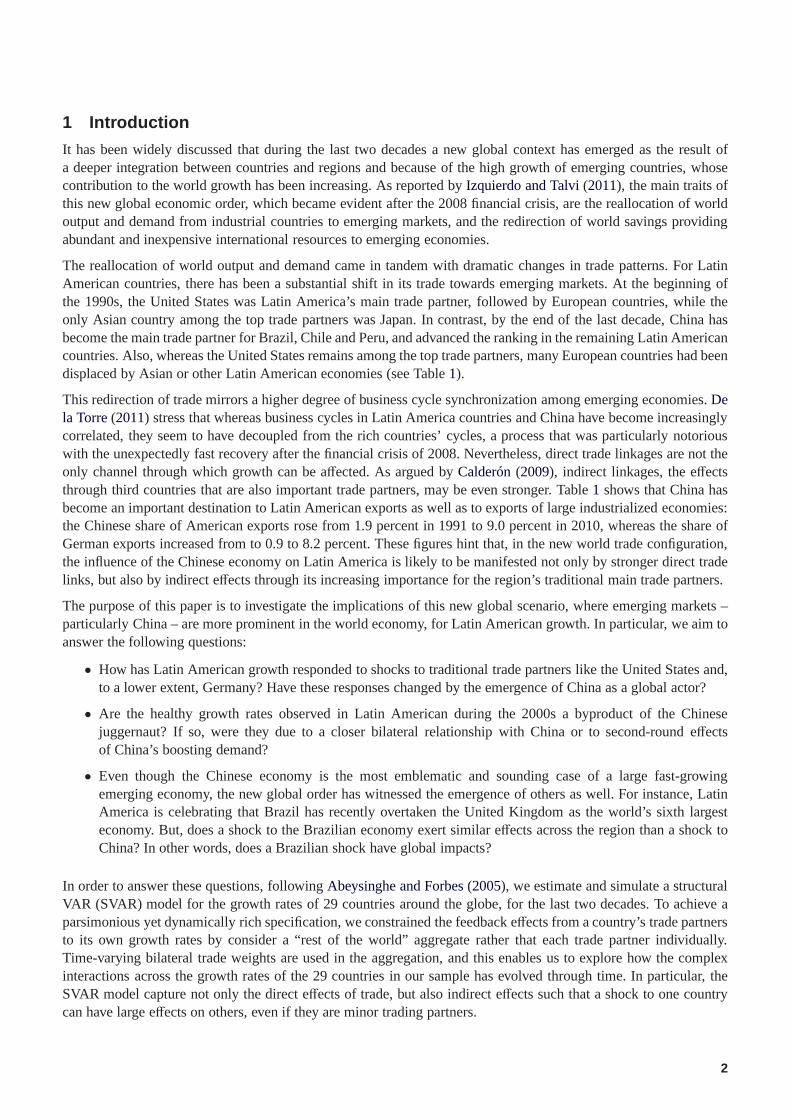
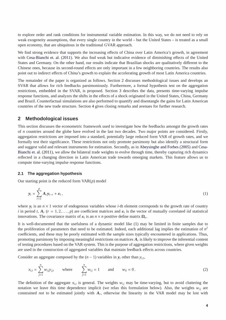
In order to quantify the transmission of external shocks to Latin American countries, and how it has changedfrom the beginning of the 1990s to the late 2000s, we conduct impulse response analyses conditional on differentconfigurations of world trade (i.e., different matricesWt). Amongst the 29 possible shocks of the system, 4 are ofparticular interest. The United States and countries of theEurozone have been traditionally the main destinations ofLatin American exports, and thus it is natural to consider a shock in the United States and a shock in Germany, as arepresentative of the Eurozone. On the other hand, one of themain focus of our empirical exploration is a shock tothe new starring actor on the world trade scene: China. Finally, it is also of interest to enquiry whether a shock tothe largest Latin American economy, Brazil, may have potential global impacts.

In a first exercise we compute the relative effectsρi j (h) of a shock on the aforementioned countries at both ends ofour sample: 1991 and 2011. Figure1 depicts the relative effects as a function ofh for both periods, with confidenceintervals constructed using a parametric bootstrap. Thereare some results to highlight:

• As expected, shocks to the United States and, to a lower extent, to Germany induce significant strongresponses in all Latin American countries. Also, these effects have changed little from 1991 to 2011: eventhough point estimates are smaller in 2011 than in 1991, often the confidence intervals at the two differentperiods overlap, thus suggesting that the difference is not statistically significant. However, the effect of anAmerican shock appears to be diminished significantly in thecase of Chile, Ecuador and Peru, whereas theeffect of a German shock is weaker in the case of Chile.

• Our estimations point out to a clear, significant increase inthe influence of the Chinese shock in the region,in agreement withCesa-Bianchi et. al.(2011). In all countries, but Venezuela, and for allh, the profile of therelative effects of the Chinese shock is significantly greater in 2011 than in 1991. The effect on impact (h = 0),which captures the changes in trade in the last two decades, has doubled, whereas the multiplier effects (h > 0)which include second-round effects of China as a global actor, has almost tripled. Furthermore, the resultsindicate that in 1991 the effects of a shock in China on Latin American were due exclusively to their tradinglinks (the response on impact is not statistically different from the response afterh quarters), whereas in 2011both the response on impact and the second-round effects increased unambiguously.

It can be appreciated that in 1991 the effects of the German shock had been statistically higher than thatof the Chinese shock. Two decades later, in 2011, the relative effect of the Chinese shock is of comparablemagnitude to that of the German shock. Moreover, the point estimates of the former appear to be higher thanthe latter, even though the differences are not yet statistically significant.

• The Brazilian shock exerts an important influence on Argentina and Uruguay, the two countries in our samplethat apart from Brazil are members of the Mercosur trading bloc. In the rest of Latin American countries,however, the effects of the Brazilian shock is comparably limited. In particular, the effect on impact (h = 0)does not seem different from the multiplier effects (h > 0), which suggest that the Brazilian shock, as opposedto the Chinese one, does not have global impacts. These results have not changed between 1991 and 2011.

In a second exercise we compute the relative effects for all quarters in the sample, to enquiry whether thedocumented changes in the influences of various shock on Latin American growth have evolved smoothly andmonotonically. Figure2 shows the resulting time profiles for selected values ofh = 0, 1, 4, 8. Recall that the directeffect of the shock is on impact, the first solid lineh = 0, and as we move through the lines representing highervalues ofh the responses are also influenced by the global effects generated by the shock.

• The results on the Chinese shock are again worth commenting on. The effect on impact has shown a sustainedupward trend since the mid 2000s, which mirrors the increasein bilateral trade with China for each countryin Table1. More interestingly, it is the second-round effects (h > 0) that display a steeper increase sincethe beginning of the 2000s, thereby capturing the importance of the Chinese shock worldwide. A tentativeconclusion is that, even though China has become one of the main trade partners of Latin American countries,it is the indirect effect of an expansion in China what affects Latin American growth the most.

10

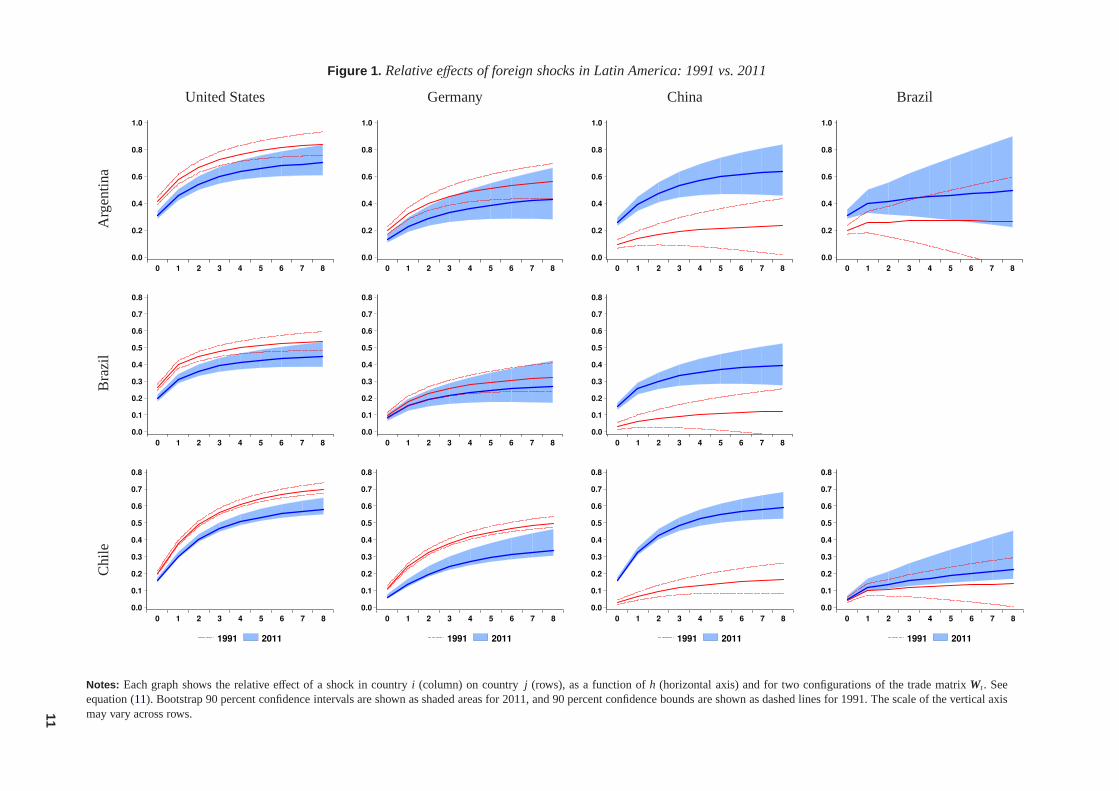
Figure 1. Relative effects of foreign shocks in Latin America: 1991 vs. 2011

United States Germany China BrazilA

rgen

tina

0.0

0.2

0.4

0.6

0.8

1.0

0 1 2 3 4 5 6 7 8

0.0

0.2

0.4

0.6

0.8

1.0

0 1 2 3 4 5 6 7 8

0.0

0.2

0.4

0.6

0.8

1.0

0 1 2 3 4 5 6 7 8

0.0

0.2

0.4

0.6

0.8

1.0

0 1 2 3 4 5 6 7 8

Bra

zil

0.0

0.1

0.2

0.3

0.4

0.5

0.6

0.7

0.8

0 1 2 3 4 5 6 7 8

0.0

0.1

0.2

0.3

0.4

0.5

0.6

0.7

0.8

0 1 2 3 4 5 6 7 8

0.0

0.1

0.2

0.3

0.4

0.5

0.6

0.7

0.8

0 1 2 3 4 5 6 7 8

Chi

le

0.0

0.1

0.2

0.3

0.4

0.5

0.6

0.7

0.8

0 1 2 3 4 5 6 7 8

1991 2011

0.0

0.1

0.2

0.3

0.4

0.5

0.6

0.7

0.8

0 1 2 3 4 5 6 7 8

1991 2011

0.0

0.1

0.2

0.3

0.4

0.5

0.6

0.7

0.8

0 1 2 3 4 5 6 7 8

1991 2011

0.0

0.1

0.2

0.3

0.4

0.5

0.6

0.7

0.8

0 1 2 3 4 5 6 7 8

1991 2011

Notes: Each graph shows the relative effect of a shock in countryi (column) on countryj (rows), as a function ofh (horizontal axis) and for two configurations of the trade matrix Wt. Seeequation (11). Bootstrap 90 percent confidence intervals are shown as shaded areas for 2011, and 90 percent confidence bounds are shownas dashed lines for 1991. The scale of the vertical axismay vary across rows.11

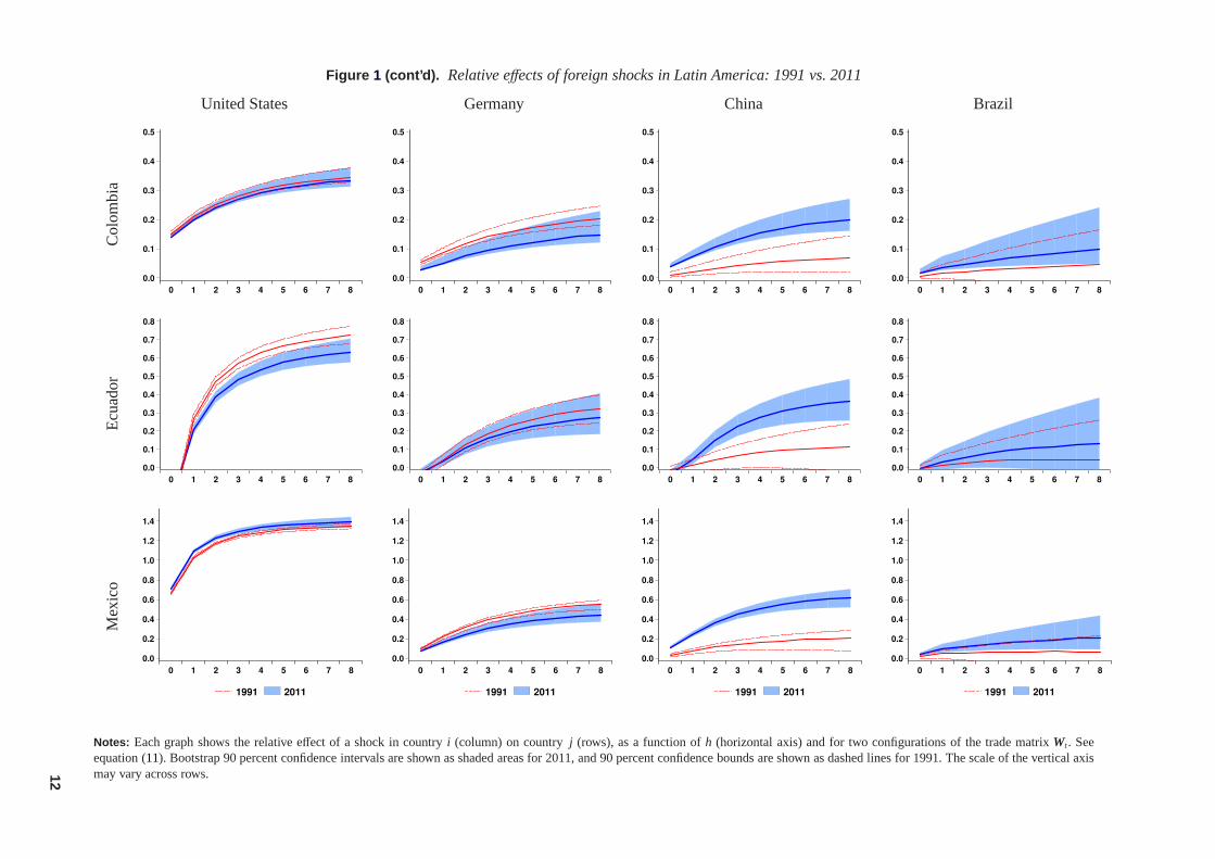
Figure 1 (cont’d). Relative effects of foreign shocks in Latin America: 1991 vs. 2011

United States Germany China BrazilC

olom

bia

0.0

0.1

0.2

0.3

0.4

0.5

0 1 2 3 4 5 6 7 8

0.0

0.1

0.2

0.3

0.4

0.5

0 1 2 3 4 5 6 7 8

0.0

0.1

0.2

0.3

0.4

0.5

0 1 2 3 4 5 6 7 8

0.0

0.1

0.2

0.3

0.4

0.5

0 1 2 3 4 5 6 7 8

Ecu

ador

0.0

0.1

0.2

0.3

0.4

0.5

0.6

0.7

0.8

0 1 2 3 4 5 6 7 8

0.0

0.1

0.2

0.3

0.4

0.5

0.6

0.7

0.8

0 1 2 3 4 5 6 7 8

0.0

0.1

0.2

0.3

0.4

0.5

0.6

0.7

0.8

0 1 2 3 4 5 6 7 8

0.0

0.1

0.2

0.3

0.4

0.5

0.6

0.7

0.8

0 1 2 3 4 5 6 7 8

Mex

ico

0.0

0.2

0.4

0.6

0.8

1.0

1.2

1.4

0 1 2 3 4 5 6 7 8

1991 2011

0.0

0.2

0.4

0.6

0.8

1.0

1.2

1.4

0 1 2 3 4 5 6 7 8

1991 2011

0.0

0.2

0.4

0.6

0.8

1.0

1.2

1.4

0 1 2 3 4 5 6 7 8

1991 2011

0.0

0.2

0.4

0.6

0.8

1.0

1.2

1.4

0 1 2 3 4 5 6 7 8

1991 2011

Notes: Each graph shows the relative effect of a shock in countryi (column) on countryj (rows), as a function ofh (horizontal axis) and for two configurations of the trade matrix Wt. Seeequation (11). Bootstrap 90 percent confidence intervals are shown as shaded areas for 2011, and 90 percent confidence bounds are shownas dashed lines for 1991. The scale of the vertical axismay vary across rows.12

Figure 1 (cont’d). Relative effects of foreign shocks in Latin America: 1991 vs. 2011

United States Germany China BrazilP

eru

0.0

0.2

0.4

0.6

0.8

1.0

1.2

0 1 2 3 4 5 6 7 8

0.0

0.2

0.4

0.6

0.8

1.0

1.2

0 1 2 3 4 5 6 7 8

0.0

0.2

0.4

0.6

0.8

1.0

1.2

0 1 2 3 4 5 6 7 8

0.0

0.2

0.4

0.6

0.8

1.0

1.2

0 1 2 3 4 5 6 7 8

Uru

guay

0.0

0.1

0.2

0.3

0.4

0.5

0.6

0.7

0.8

0 1 2 3 4 5 6 7 8

0.0

0.1

0.2

0.3

0.4

0.5

0.6

0.7

0.8

0 1 2 3 4 5 6 7 8

0.0

0.1

0.2

0.3

0.4

0.5

0.6

0.7

0.8

0 1 2 3 4 5 6 7 8

0.0

0.1

0.2

0.3

0.4

0.5

0.6

0.7

0.8

0 1 2 3 4 5 6 7 8

Ven

ezue

la

0.0

0.1

0.2

0.3

0.4

0.5

0.6

0.7

0.8

0 1 2 3 4 5 6 7 8

1991 2011

0.0

0.1

0.2

0.3

0.4

0.5

0.6

0.7

0.8

0 1 2 3 4 5 6 7 8

1991 2011

0.0

0.1

0.2

0.3

0.4

0.5

0.6

0.7

0.8

0 1 2 3 4 5 6 7 8

1991 2011

0.0

0.1

0.2

0.3

0.4

0.5

0.6

0.7

0.8

0 1 2 3 4 5 6 7 8

1991 2011

Notes: Each graph shows the relative effect of a shock in countryi (column) on countryj (rows), as a function ofh (horizontal axis) and for two configurations of the trade matrix Wt. Seeequation (11). Bootstrap 90 percent confidence intervals are shown as shaded areas for 2011, and 90 percent confidence bounds are shownas dashed lines for 1991. The scale of the vertical axismay vary across rows.13

The time profile of the relative effects also uncovers interesting dynamics in the responses tothe Chineseshock. Forh > 0, its influence declines from 1998 to 2002, whereas the direct effect inh = 0 remains stable.This combination seems to be a consequence of the 1997 Asian financial crisis. Whereas it barely changedthe bilateral relationships of Latin American countries with China, it hit hardly many of China’s main tradepartners. Hence, the trade amongst Asian economies shrunk and this phenomenon weakened the channelwhereby shocks in China’s growth were propagated around theglobe (seeAbeysinghe and Forbes, 2005).

• On the other hand, we observe that in the case of the American shock, the relative effects both on impact andindirect have remained mostly unchanged. However, the responses of Argentina, Chile, Peru and Uruguayafter the 2008 financial crisis, reflect not only a modest shrinkage in the trade share of the United States, butmore importantly somehow weaker second-round effects of an American shock.

As concluded in the analysis of Figure1, many of these changes are not statistically significant; nonetheless,if the movements observed by the end of the sample are an indication of a downward trend developing, it willnot be long until a significant reduction in the importance ofthe American shock can be reported. In fact, thisis the case of the responses to the German shock whose influence has shown a steady (albeit modest) declinesince the mid 1990s, and for all the Latin American countriesin the sample.

• Finally, the relative effects of a Brazilian shock display a hump between the mid 1990sto the mid 2000s,which is very pronounced for Mercosur members but is buffered for the remaining Latin American countries(notably Chile, that have important direct trade linkages with Mercosur economies). Outside Mercosur,however, the relative effects of a Brazilian perturbation are basically reflected by the direct impacts on trade,their second-round effects seem insignificant and very stable through time.

3.4 Direct vs. indirect effects: Counterfactual simulations

Our previous results point out to two important conclusions. Firstly, the changing trading structure of LatinAmerican countries has promoted growth as it was oriented towards fast-growing economies, remarkably China.Secondly, second-round effects of the outstanding Chinese growth in the 2000s has constituted a relevant source ofgrowth in the region.

Unfortunately, with the exception of the relative effects (11) on impact (h = 0), for h > 0 the analysis so far does notdisentangle the direct effect of changing the trade structure from the indirect ones. Next, we perform counterfactualsimulations in order to have a better grasp of the relative importance of these effects. In particular, using the actualestimated structural shocksut, the SVAR is simulated for the period 2006 to 2011 (the 2008 financial crisis occurredin the middle of this window), under different assumptions regarding the world trade structure, seeequation (9):

• First, for all t in the simulation window, the matrixWt is set equal to its average value over that period (W2).

The result is a set of growth rates that are close, but greaterthan the actual values. Compare the first and sixthcolumns of Table3: an average of 5.51 percent versus and 4.94 percent. The reason for this discrepancy is that,in the simulations, although the upward trending export weights of Latin American countries with boomingemerging markets are replaced with greater shares at the beginning of the simulation and with smaller sharesby the end, the effects on growth are not compensated because of more favorableinitial conditions. Therefore,the counterfactual set, i.e. the sixth column of Table3, is used as a baseline scenario for comparative purposes.

• Second, the trade matrixWt is replaced by its average value over 1994 to 2000 (W1).

This situation corresponds to a trade structure before China’s emergence as a global actor, and the resultsare given in the second column of Table3. On average, Latin American growth amounts to a modest 2.94percent, almost half of the growth obtained in the baseline scenario. The difference between scenarios (2.57percent) gives the overall effect of the changing trade structure on growth, and is reported in the fifth columnof Table3.

• Finally, an intermediate configuration is considered in order to assess the direct effects of the new tradestructure on growth (W3). The idea is to let Latin American’s trade structure evolve, while keeping the

14

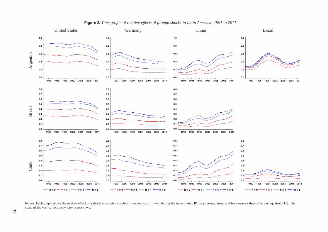
Figure 2. Time profile of relative effects of foreign shocks in Latin America: 1991 to 2011

United States Germany China BrazilA

rgen

tina

0.0

0.2

0.4

0.6

0.8

1.0

1993 1996 1999 2002 2005 2008 2011

0.0

0.2

0.4

0.6

0.8

1.0

1993 1996 1999 2002 2005 2008 2011

0.0

0.2

0.4

0.6

0.8

1.0

1993 1996 1999 2002 2005 2008 2011

0.0

0.2

0.4

0.6

0.8

1.0

1993 1996 1999 2002 2005 2008 2011

Bra

zil

0.0

0.1

0.2

0.3

0.4

0.5

0.6

0.7

0.8

1993 1996 1999 2002 2005 2008 2011

0.0

0.1

0.2

0.3

0.4

0.5

0.6

0.7

0.8

1993 1996 1999 2002 2005 2008 2011

0.0

0.1

0.2

0.3

0.4

0.5

0.6

0.7

0.8

1993 1996 1999 2002 2005 2008 2011

Chi

le

0.0

0.1

0.2

0.3

0.4

0.5

0.6

0.7

0.8

1993 1996 1999 2002 2005 2008 2011

h = 0 h = 1 h = 4 h = 8

0.0

0.1

0.2

0.3

0.4

0.5

0.6

0.7

0.8

1993 1996 1999 2002 2005 2008 2011

h = 0 h = 1 h = 4 h = 8

0.0

0.1

0.2

0.3

0.4

0.5

0.6

0.7

0.8

1993 1996 1999 2002 2005 2008 2011

h = 0 h = 1 h = 4 h = 8

0.0

0.1

0.2

0.3

0.4

0.5

0.6

0.7

0.8

1993 1996 1999 2002 2005 2008 2011

h = 0 h = 1 h = 4 h = 8

Notes: Each graph shows the relative effect of a shock in countryi (column) on countryj (rows), letting the trade matrixWt vary through time, and for various values ofh. See equation (11). Thescale of the vertical axis may vary across rows.15

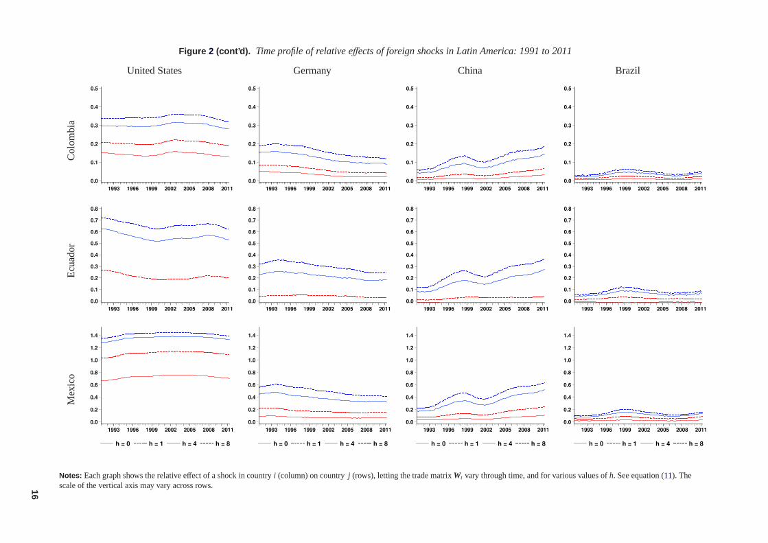
Figure 2 (cont’d). Time profile of relative effects of foreign shocks in Latin America: 1991 to 2011

United States Germany China BrazilC

olom

bia

0.0

0.1

0.2

0.3

0.4

0.5

1993 1996 1999 2002 2005 2008 2011

0.0

0.1

0.2

0.3

0.4

0.5

1993 1996 1999 2002 2005 2008 2011

0.0

0.1

0.2

0.3

0.4

0.5

1993 1996 1999 2002 2005 2008 2011

0.0

0.1

0.2

0.3

0.4

0.5

1993 1996 1999 2002 2005 2008 2011

Ecu

ador

0.0

0.1

0.2

0.3

0.4

0.5

0.6

0.7

0.8

1993 1996 1999 2002 2005 2008 2011

0.0

0.1

0.2

0.3

0.4

0.5

0.6

0.7

0.8

1993 1996 1999 2002 2005 2008 2011

0.0

0.1

0.2

0.3

0.4

0.5

0.6

0.7

0.8

1993 1996 1999 2002 2005 2008 2011

0.0

0.1

0.2

0.3

0.4

0.5

0.6

0.7

0.8

1993 1996 1999 2002 2005 2008 2011

Mex

ico

0.0

0.2

0.4

0.6

0.8

1.0

1.2

1.4

1993 1996 1999 2002 2005 2008 2011

h = 0 h = 1 h = 4 h = 8

0.0

0.2

0.4

0.6

0.8

1.0

1.2

1.4

1993 1996 1999 2002 2005 2008 2011

h = 0 h = 1 h = 4 h = 8

0.0

0.2

0.4

0.6

0.8

1.0

1.2

1.4

1993 1996 1999 2002 2005 2008 2011

h = 0 h = 1 h = 4 h = 8

0.0

0.2

0.4

0.6

0.8

1.0

1.2

1.4

1993 1996 1999 2002 2005 2008 2011

h = 0 h = 1 h = 4 h = 8

Notes: Each graph shows the relative effect of a shock in countryi (column) on countryj (rows), letting the trade matrixWt vary through time, and for various values ofh. See equation (11). Thescale of the vertical axis may vary across rows.16

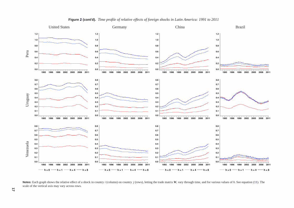
Figure 2 (cont’d). Time profile of relative effects of foreign shocks in Latin America: 1991 to 2011

United States Germany China BrazilP

eru

0.0

0.2

0.4

0.6

0.8

1.0

1.2

1993 1996 1999 2002 2005 2008 2011

0.0

0.2

0.4

0.6

0.8

1.0

1.2

1993 1996 1999 2002 2005 2008 2011

0.0

0.2

0.4

0.6

0.8

1.0

1.2

1993 1996 1999 2002 2005 2008 2011

0.0

0.2

0.4

0.6

0.8

1.0

1.2

1993 1996 1999 2002 2005 2008 2011

Uru

guay

0.0

0.1

0.2

0.3

0.4

0.5

0.6

0.7

0.8

1993 1996 1999 2002 2005 2008 2011

0.0

0.1

0.2

0.3

0.4

0.5

0.6

0.7

0.8

1993 1996 1999 2002 2005 2008 2011

0.0

0.1

0.2

0.3

0.4

0.5

0.6

0.7

0.8

1993 1996 1999 2002 2005 2008 2011

0.0

0.1

0.2

0.3

0.4

0.5

0.6

0.7

0.8

1993 1996 1999 2002 2005 2008 2011

Ven

ezue

la

0.0

0.1

0.2

0.3

0.4

0.5

0.6

0.7

0.8

1993 1996 1999 2002 2005 2008 2011

h = 0 h = 1 h = 4 h = 8

0.0

0.1

0.2

0.3

0.4

0.5

0.6

0.7

0.8

1993 1996 1999 2002 2005 2008 2011

h = 0 h = 1 h = 4 h = 8

0.0

0.1

0.2

0.3

0.4

0.5

0.6

0.7

0.8

1993 1996 1999 2002 2005 2008 2011

h = 0 h = 1 h = 4 h = 8

0.0

0.1

0.2

0.3

0.4

0.5

0.6

0.7

0.8

1993 1996 1999 2002 2005 2008 2011

h = 0 h = 1 h = 4 h = 8

Notes: Each graph shows the relative effect of a shock in countryi (column) on countryj (rows), letting the trade matrixWt vary through time, and for various values ofh. See equation (11). Thescale of the vertical axis may vary across rows.17

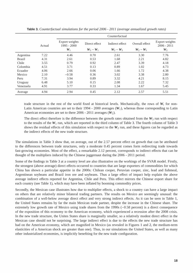
Table 3. Counterfactual simulations for the period 2006 - 2011 (average annualized growth rates)

Counterfactual

Export weightsDirect effect Indirect effect Overall effect

Export weightsActual 1995 - 2000 2006 - 2011

W1 W3 −W1 W2 −W3 W2 −W1 W2

Argentina 7.22 4.46 0.70 2.61 3.30 7.76Brazil 4.31 2.61 0.53 1.68 2.21 4.82Chile 3.55 0.79 0.92 2.47 3.39 4.18Colombia 4.51 3.71 0.13 0.89 1.02 4.73Ecuador 4.06 2.66 0.06 1.66 1.72 4.38Mexico 2.10 −0.58 0.36 3.02 3.38 2.80Peru 7.31 3.94 0.89 3.32 4.21 8.15Uruguay 6.48 5.10 0.15 2.08 2.22 7.32Venezuela 4.91 3.77 0.33 1.34 1.67 5.45

Average 4.94 2.94 0.45 2.12 2.57 5.51

trade structure in the rest of the world fixed at historical levels. Mechanically, the rows ofWt for non-Latin American countries are set to their 1994 - 2000 averages (W1), whereas those corresponding to LatinAmerican economies are set to there 2006 - 2011 averages (W2).

The direct effect therefore is the difference between the growth rates obtained from theW3 run with respectto the results of theW1 run, which are reported in the third column of Table3. The fourth column of Table3shows the residual effects of this simulation with respect to theW2 run, and these figures can be regarded asthe indirect effects of the new trade structure.

The simulations in Table3 show that, on average, out of the 2.57 percent effect on growth that can be attributedto the differences between trade structures, only a moderate 0.45 percent comes form redirecting trade towardsfast-growing economies. Most of the effect, a remarkable 2.12 percent, corresponds to indirect effects that can bethought of the multipliers induced by the Chinese juggernaut during the 2006 - 2011 period.

Some of the findings in Table3 at a country level are also illustrative on the workings of the SVAR model. Firstly,the strongest (above average) direct effects occurred to countries that are large exporters of commodities for whichChina has shown a particular appetite in the 2000s: Chilean cooper, Peruvian cooper, zinc, lead and fishmeal,Argentinean soybeans and Brazil iron ore and soybeans. Thusa large effect of impact help explain the aboveaverage indirect effects reported for Argentina, Chile and Peru. This effect mirrors the Chinese export share foreach country (see Table1), which may have been inflated by booming commodity prices.

Secondly, the Mexican case illustrates how due to multiplier effects, a shock to a country can have a large impacton others that are relatively minor bilateral trading partners. The results on Mexico are seemingly unusual: thecombination of a well-below average direct effect and very strong indirect effects. As it can be seen in Table1,the United States remains by far the main Mexican trade partner, despite the increase in the Chinese share. Theextremely low growth rate of Mexico using trade shares from the 1990s (−0.58 percent) is a direct consequenceof the exposition of this economy to the American economy, which experienced a recession after the 2008 crisis.In the new trade structure, the Unites States share is marginally smaller, so a relatively modest direct effect in theMexican case should not be surprising. The large indirect effect is due to the effects the new trade structure hashad on the American economy, which are magnified in Mexico (asrevealed in Figures1 and2, the medium-termelasticities of a American shock are greater than one). Thus, in our simulations the United States, as well as manyother industrialized economies, is implicitly benefiting for the new trade configuration.

18

4 Concluding remarks

In this paper we have developed a SVAR model with rich feedbacks, direct and indirect, for 29 economiesworldwide. Aggregation restrictions using trade shares are formally tested and then imposed to achieve both arather parsimonious system and the identification of a structural form. As the trade shares are time-varying, soare the impulse-response function of the SVAR, which enables us to analyze the changes that the effects on LatinAmerican growth of shocks in the United States, China, Germany and Brazil, have undergone.

Our results point out to relatively stable effects on Latin American growth of shocks in the United States,althoughthey seem to have diminished by the end of our sample. In contrast, the indirect effects of a German shock havereduced steadily during the last decade, somehow displacedby particularly strong indirect effects of a Chineseshock. These findings support the idea that the more prominent presence of China in the world economic scenehave had a potentially large impact on third countries, evenif they are minor trade partners.

Counterfactual simulations show that a remarkable proportion of the vigorous Latin American growth experiencedin the period 2006 - 2011 can be attributed to second-round effects, while only a modest fraction is due to changingtrade orientation towards fast-growing emerging economies. These findings have profound policy implications. Wereckon that part of the direct effect may be the outcome of well-suited trade policies, i.e. selecting as trade partners(for instance, through the enactment of formal trade agreements) those economies that can sustain the demandfor the products for which a country has comparative advantages. Yet, we estimate that these policies would havegranted Latin American countries an increase of (at most) 0.5 percent in its growth rate. This is a significant resultbut may not be enough to move towards a sustainable high growth path.

On the other hand, most Latin American counties remain rather small open economies, simply spectators of theworld economic scene. Our results point out that even Brazil, despite its size, is still unavailable of influencing thedynamics of economies beyond the region. As a whole, Latin America still seems vulnerable to external shocks, sothat the strong positive indirect effect on growth reported above, can be regarded as sheer “good luck” (a particularlygood realization of shocks). It is, therefore, a core policychallenge for each Latin American country to seize onsuch favorable external conditions, which albeit persistent are likely to be temporary, to promote policies aimed toreduce its vulnerability to foreign shocks.

There are several ways in which China may have affected Latin America: commercial, financial and by sustaininghigh commodities prices in international markets. Even though some emphasis was given to the commercialchannel, we have not truly attempted to make a distinction among these channels and we reckon do it so constitutesan interesting avenue for future research. In particular, to explicitly model and quantify the effects of Chinesedemand on the terms of trade of commodity exporters, such as most Latin American countries (see, for instance,Abeysinghe, 2001). Another interesting extension is to assess the effects of global shocks (for instance, byconsidering the presence of common factors in the structural perturbations), and especially to enquire whetherthe redirection of trade towards emerging markets has delivered the diversification gains that theory predicts.

References

Abeysinghe, T. (2001), “Estimation of direct and indirect impact of oil price on growth”,Economics Letters, 73(2),147–153.

Abeysinghe, T. and K. Forbes (2005), “Trade linkages and output-multiplier effects: A structural VAR approachwith a focus on Asia”,Review of International Economics, 13(2), 356-375.

Abeysinghe, T. and R. Gulasekaran (2004), “Quarterly real GDP estimates for China and ASEAN4 with a forecastevaluation”,Journal of Forecasting, 23(6), 431-447.

Canova, F. (2005), “The transmission of US shocks to Latin America”, Journal of Applied Econometrics, 20(2),229-251.

Canova F. and M. Ciccarelli (2009), “Estimating multicountry VAR models”, International Economic Review,50(3), 929-959.

19

Calderón, C. (2009) “Trade, specialization, and cycle synchronization: Explaining output comovement betweenLatin America, China, and India”, in Lederman, D., M. Olarreaga and G. E. Perry (eds.),China’s and India’schallenge to Latin Ameica: Opportunity or threat?, The World Bank, ch. 2, 39-100.

Cesa-Bianchi, A., M. H. Pesaran, A. Rebucci and T. Xu (2011),“China’s emergence in the world economy andbusiness cycles in Latin America”, Inter-American Development Bank working paper IDB-WP-266.

De la Torre, A. (2011), ”LAC succes put to the test”, speech delivered at the Central Reserve Bank of Peru, August15, 2011. Available athttp://www.bcrp.gob.pe

Dees, S., F. di Mauro, H. M. Pesaran and L. V. Smith (2007), “Exploring the international linkages of the Euro area:A global VAR analysis”,Journal of Applied Econometrics, 22(1), 1-38.

Elliott, G. and A. Fatas (1996), “International business cycles and the dynamics of the current account”,EuropeanEconomic Review, 40(2), 361-387.

Enders, W. and K. Souki (2008), “Assesing the importance of global shocks versus country-specific shocks”,Journal of International Money and Finance, 27(8), 1420-1429.

Forbes, K. and M. Chinn (2004), “A decomposition of global linkages in financial markets over time”,Review ofEconomics and Statistics, 86(3), 705-722.

Glick, R. and K. Rogoff (1995), “Global versus country-specific productivity shocks and the current account”,Journal of Monetary Economics, 35(1), 159-192.

Hurvich, C. M. and C. Tsai (1989), “Regression and time series model selection in small samples”,Biometrika,76(2), 297-307.

Izquierdo, A. and E. Talvi (2011), “What’s next? Latin America and the Caribbean’s insertion into the post-financialcrisis new global economic order”, in Izquierdo, A. and E. Talvi (eds.),One Region, Two Speeds? Challengesof the New Economic Order for Latin America and the Caribbean, Inter-American Development Bank, ch. 2,15-29.

Mutl, J. (2009), “Consistent estimation of global VAR models”, Institute for Advanced Studies (Vienna), EconomicsSeries 234.

Norrbin, S. C. and D. E. Schlagenhauf (1996), “The role of international factors in the business cycle: A multi-country study”,Journal of International Economics, 40(1-2), 85-104.

Pesaran, M. H., T. Schuermann and S. M. Weiner (2004), “Modeling regional interdependencies using a globalerror-correcting macroeconometric model”,Journal of Business and Economic Statistics, 22(2), 129-162.

Primiceri, G. (2005), “Time varying structural vector autoregressions and monetary policy”,Review of EconomicStudies, 72, 821-852.

Winkelried, D. (2011), “Exchange rate pass through and inflation targeting in Peru”, Central Reserve Bank of Peru,Working Paper 2011-12.

20