Trade, Inequality and Costly Redistributionitskhoki/papers/TradeInequalityRedistribution... · A Motivating Example Economic Model Calibration and Counterfactuals Trade, Inequality

A Motivating ExampleEconomic Model

Calibration and Counterfactuals

Trade, Inequality and Costly Redistribution

Pol AntrasHarvard University

Alonso de GortariHarvard University

Oleg ItskhokiPrinceton University

London School of EconomicsMay 8, 2015

Antras, de Gortari and Itskhoki Trade, Inequality and Costly Redistribution 1 / 46



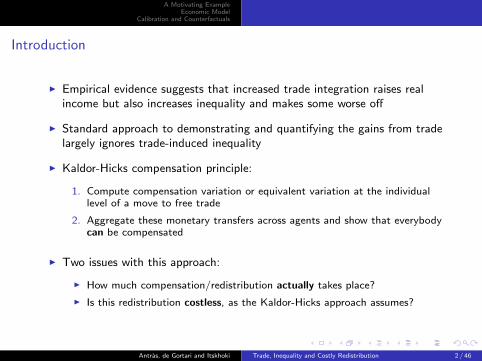
Introduction

I Empirical evidence suggests that increased trade integration raises realincome but also increases inequality and makes some worse off

I Standard approach to demonstrating and quantifying the gains from tradelargely ignores trade-induced inequality

I Kaldor-Hicks compensation principle:

1. Compute compensation variation or equivalent variation at the individuallevel of a move to free trade

2. Aggregate these monetary transfers across agents and show that everybodycan be compensated

I Two issues with this approach:

I How much compensation/redistribution actually takes place?

I Is this redistribution costless, as the Kaldor-Hicks approach assumes?




This Paper

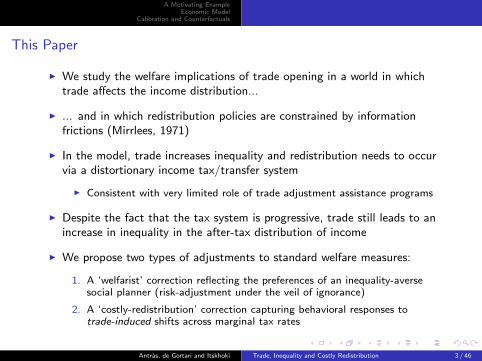
I We study the welfare implications of trade opening in a world in whichtrade affects the income distribution...

I ... and in which redistribution policies are constrained by informationfrictions (Mirrlees, 1971)

I In the model, trade increases inequality and redistribution needs to occurvia a distortionary income tax/transfer system

I Consistent with very limited role of trade adjustment assistance programs

I Despite the fact that the tax system is progressive, trade still leads to anincrease in inequality in the after-tax distribution of income

I We propose two types of adjustments to standard welfare measures:

1. A ‘welfarist’ correction reflecting the preferences of an inequality-aversesocial planner (risk-adjustment under the veil of ignorance)

2. A ‘costly-redistribution’ correction capturing behavioral responses totrade-induced shifts across marginal tax rates




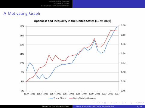
A Motivating Graph

0.46

0.48

0.50

0.52

0.54

0.56

0.58

0.60

7%

8%

9%

10%

11%

12%

13%

14%

1979 1981 1983 1985 1987 1989 1991 1993 1995 1997 1999 2001 2003 2005 2007

Openness and Inequality in the United States (1979‐2007)

Trade Share Gini of Market Income




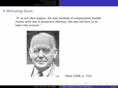
A Motivating Quote

“If, as will often happen, the best methods of compensation feasibleinvolve some loss in productive efficiency, this loss will have to betaken into account.”

Hicks (1939, p. 712)




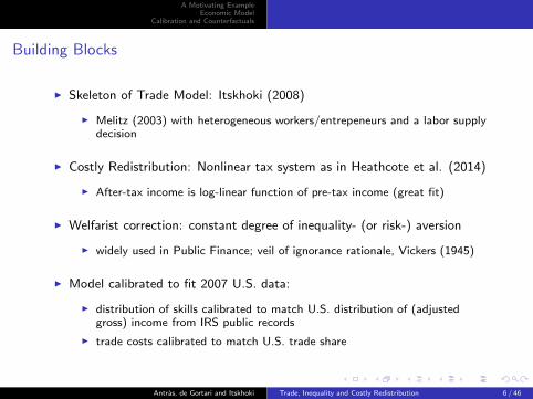
Building Blocks

I Skeleton of Trade Model: Itskhoki (2008)

I Melitz (2003) with heterogeneous workers/entrepeneurs and a labor supplydecision

I Costly Redistribution: Nonlinear tax system as in Heathcote et al. (2014)

I After-tax income is log-linear function of pre-tax income (great fit)

I Welfarist correction: constant degree of inequality- (or risk-) aversion

I widely used in Public Finance; veil of ignorance rationale, Vickers (1945)

I Model calibrated to fit 2007 U.S. data:

I distribution of skills calibrated to match U.S. distribution of (adjustedgross) income from IRS public records

I trade costs calibrated to match U.S. trade share




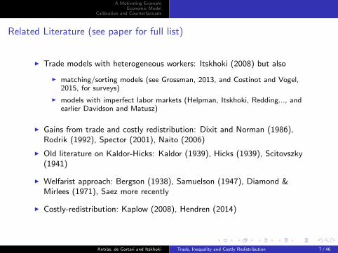
Related Literature (see paper for full list)

I Trade models with heterogeneous workers: Itskhoki (2008) but also

I matching/sorting models (see Grossman, 2013, and Costinot and Vogel,2015, for surveys)

I models with imperfect labor markets (Helpman, Itskhoki, Redding..., andearlier Davidson and Matusz)

I Gains from trade and costly redistribution: Dixit and Norman (1986),Rodrik (1992), Spector (2001), Naito (2006)

I Old literature on Kaldor-Hicks: Kaldor (1939), Hicks (1939), Scitovszky(1941)

I Welfarist approach: Bergson (1938), Samuelson (1947), Diamond &Mirlees (1971), Saez more recently

I Costly-redistribution: Kaplow (2008), Hendren (2014)




Road Map

1. A Motivating Example

2. Economic Model

3. Calibration

4. Counterfactuals: Inequality and the Gains from Trade




Kaldor-Hicks PrincipleWelfarist CorrectionCostly Redistribution Correction

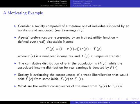
A Motivating Example

I Consider a society composed of a measure one of individuals indexed by anability ϕ and associated (real) earnings r (ϕ)

I Agents’ preferences are represented by an indirect utility function vdefined over (real) disposable income

rd (ϕ) = (1− τ (r (ϕ))) r (ϕ) + T (ϕ)

where τ (r) is a nonlinear income tax and T (ϕ) a lump-sum transfer

I The cumulative distribution of ϕ in the population is H (ϕ), while theassociated income distribution for real earnings is denoted by F (r)

I Society is evaluating the consequences of a trade liberalization that wouldshift F (r) from some initial F0 (r) to F1 (r).

I What are the welfare consequences of the move from F0 (r) to F1 (r)?





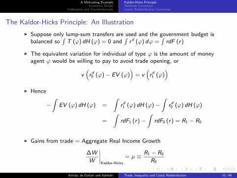
The Kaldor-Hicks Principle: An Illustration

I Suppose only lump-sum transfers are used and the government budget isbalanced so

∫T (ϕ) dH (ϕ) = 0 and

∫rd (ϕ) dϕ =

∫rdF (r)

I The equivalent variation for individual of type ϕ is the amount of moneyagent ϕ would be willing to pay to avoid trade opening, or

v(rd0 (ϕ)− EV (ϕ)

)= v

(rd1 (ϕ)

)I Hence

−∫

EV (ϕ) dH (ϕ) =

∫rd1 (ϕ) dH (ϕ)−

∫rd0 (ϕ) dH (ϕ)

=

∫rdF1 (r)−

∫rdF0 (r) = R1 − R0

I Gains from trade = Aggregate Real Income Growth

∆W

W

∣∣∣∣Kaldor-Hicks

= µ ≡ R1 − R0

R0





Pros and Cons of the Kaldor-Hicks Principle

I Principle does not rely on interpersonal comparisons of utility

I indirect utility can be heterogeneous across agentsI result relies on ordinal rather than cardinal preferencesI notion of efficiency argued to be free of value judgments

I What if redistribution does not take place and the losers are notcompensated?

I under the veil of ignorance, agents will see a probability distribution overpotential outcomes

I VN-M preferences over these lotteries are necessarily cardinalI risk aversion ≈ inequality aversion

I Even if some redistribution takes place, whenever it is costly, shouldn’t∆W /W reflect those costs?

I Dixit and Norman (1986) showed that ∆W /W > 0 using a course set oftax policies - but by how much is ∆W /W diminished?





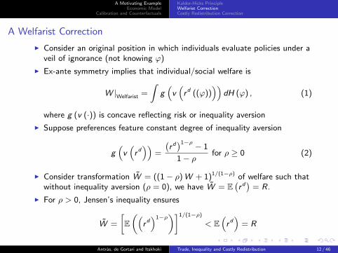
A Welfarist Correction

I Consider an original position in which individuals evaluate policies under aveil of ignorance (not knowing ϕ)

I Ex-ante symmetry implies that individual/social welfare is

W |Welfarist =

∫g(v(rd ((ϕ))

))dH (ϕ) , (1)

where g (v (·)) is concave reflecting risk or inequality aversion

I Suppose preferences feature constant degree of inequality aversion

g(v(rd))

=

(rd)1−ρ − 1

1− ρ for ρ ≥ 0 (2)

I Consider transformation W = ((1− ρ)W + 1)1/(1−ρ) of welfare such thatwithout inequality aversion (ρ = 0), we have W = E

(rd)

= R.

I For ρ > 0, Jensen’s inequality ensures

W =

[E((

rd)1−ρ

)]1/(1−ρ)

< E(rd)

= R





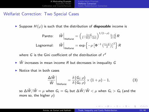
Welfarist Correction: Two Special Cases

I Suppose H (ϕ) is such that the distribution of disposable income is

Pareto: W∣∣∣

Welfarist=(

1+G1−G(1−2ρ)

)1/(1−ρ)1−G1+G

R

Lognormal: W∣∣∣

Welfarist= exp

{−ρ[Φ−1

(1+G

2

)]2}R

where G is the Gini coefficient of the distribution of rd

I W increases in mean income R but decreases in inequality G

I Notice that in both cases

∆W

W

∣∣∣∣Welfarist

=δ (G1; ρ)

δ (G0; ρ)× (1 + µ)− 1, (3)

so ∆W /W = µ when G1 = G0 but ∆W /W < µ when G1 > G0 (and themore so, the higher ρ)





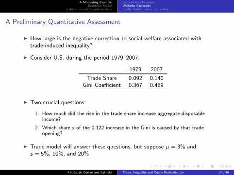
A Preliminary Quantitative Assessment

I How large is the negative correction to social welfare associated withtrade-induced inequality?

I Consider U.S. during the period 1979–2007:

1979 2007

Trade Share 0.092 0.140Gini Coefficient 0.367 0.489

I Two crucial questions:

1. How much did the rise in the trade share increase aggregate disposableincome?

2. Which share s of the 0.122 increase in the Gini is caused by that tradeopening?

I Trade model will answer these questions, but suppose µ = 3% ands = 5%, 10%, and 20%





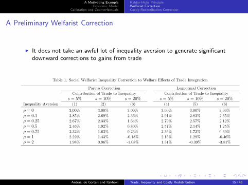
A Preliminary Welfarist Correction

I It does not take an awful lot of inequality aversion to generate significantdownward corrections to gains from trade

Table 1. Social Welfarist Inequality Correction to Welfare Effects of Trade Integration

Pareto Correction Lognormal CorrectionContribution of Trade to Inequality Contribution of Trade to Inequality

s = 5% s = 10% s = 20% s = 5% s = 10% s = 20%Inequality Aversion (1) (2) (3) (4) (5) (6)

ρ = 0 3.00% 3.00% 3.00% 3.00% 3.00% 3.00%ρ = 0.1 2.85% 2.69% 2.36% 2.91% 2.83% 2.65%ρ = 0.25 2.67% 2.33% 1.64% 2.79% 2.57% 2.12%ρ = 0.5 2.46% 1.92% 0.80% 2.57% 2.14% 1.25%ρ = 0.75 2.32% 1.63% 0.23% 2.36% 1.72% 0.39%ρ = 1 2.22% 1.43% -0.18% 2.15% 1.29% -0.46%ρ = 2 1.98% 0.96% -1.08% 1.31% -0.39% -3.81%

1





A Costly Redistribution Correction

I Suppose now that lump-sum transfers are not feasible (i.e., T (ϕ) = 0 forall ϕ) and redistribution has to happen through the income tax/transfersystem

I Focus on the particular case (as in Heathcoate et al., 2014) in which

1− τ (r (ϕ)) = k (r (ϕ))−φ , (4)

for some constant k which can be set to ensure that the governmentbudget is balanced

I Average net-of-tax rates decrease in reported income at a constant rate φ,which captures the degree of progressivity of the tax system

I Behavioral response to taxation: positive, constant elasticity of reportedincome to the net-of-tax rate, or

ε ≡ ∂r (ϕ)

∂ (1− τ (r (ϕ)))

1− τ (r (ϕ))

r (ϕ)> 0 (5)





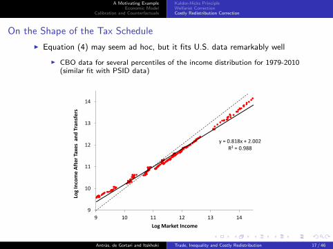
On the Shape of the Tax Schedule

I Equation (4) may seem ad hoc, but it fits U.S. data remarkably well

I CBO data for several percentiles of the income distribution for 1979-2010(similar fit with PSID data)

y = 0.818x + 2.002 R² = 0.988

9

10

11

12

13

14

9 10 11 12 13 14

Log

Inco

me

Afte

r Tax

es a

nd T

rans

fers

Log Market Income





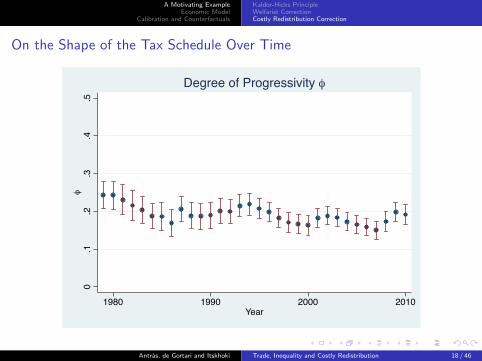
On the Shape of the Tax Schedule Over Time

0.1

.2.3

.4.5

φ

1980 1990 2000 2010Year

Degree of Progressivity φ





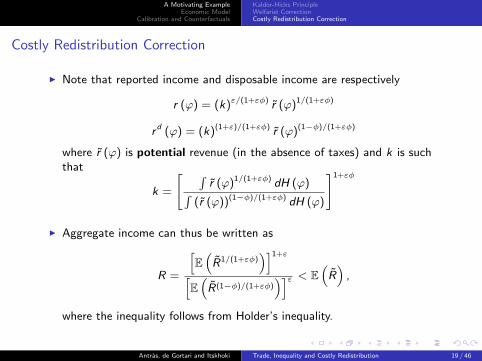
Costly Redistribution Correction

I Note that reported income and disposable income are respectively

r (ϕ) = (k)ε/(1+εφ) r (ϕ)1/(1+εφ)

rd (ϕ) = (k)(1+ε)/(1+εφ) r (ϕ)(1−φ)/(1+εφ)

where r (ϕ) is potential revenue (in the absence of taxes) and k is suchthat

k =

[ ∫r (ϕ)1/(1+εφ) dH (ϕ)∫

(r (ϕ))(1−φ)/(1+εφ) dH (ϕ)

]1+εφ

I Aggregate income can thus be written as

R =

[E(R1/(1+εφ)

)]1+ε

[E(R(1−φ)/(1+εφ)

)]ε < E(R)

,

where the inequality follows from Holder’s inequality.





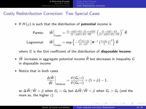
Costly Redistribution Correction: Two Special Cases

I If H (ϕ) is such that the distribution of potential income is

Pareto: W∣∣∣

Costly= (1−φ)(1+G)−(1+εφ)2G

(1−φ)(1+G)−2G

((1−φ)(1−G)

(1−φ)(1+G)−2G

)εR

Lognormal: W∣∣∣

Costly= exp

{−φ

2ε(ε+1)

(1−φ)2

[Φ−1

(1+G1

2

)]2}R

where G is the Gini coefficient of the distribution of disposable income.

I W increases in aggregate potential income R but decreases in inequality Gin disposable income

I Notice that in both cases

∆W

W

∣∣∣∣Welfarist

=θ (G1; ε)

θ (G0; ε)× (1 + µ)− 1,

so ∆W /W = µ when G1 = G0 but ∆W /W < µ when G1 > G0 (and themore so, the higher ε)





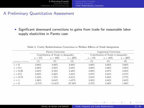
A Preliminary Quantitative Assessment

I Significant downward corrections to gains from trade for reasonable laborsupply elasticities in Pareto case

Table 2. Costly Redistribution Correction to Welfare Effects of Trade Integration

Pareto Correction Lognormal CorrectionContribution of Trade to Inequality Contribution of Trade to Inequality

s = 5% s = 10% s = 20% s = 5% s = 10% s = 20%In e q u a l i ty A v e r s io n (1) (2) (3) (4) (5) (6)

ε = 0 3.00% 3.00% 3.00% 3.00% 3.00% 3.00%ε = 0.1 2.96% 2.92% 2.83% 3.00% 2.99% 2.98%ε = 0.25 2.88% 2.76% 2.49% 2.99% 2.97% 2.95%ε = 0.5 2.69% 2.36% 1.63% 2.97% 2.94% 2.87%ε = 0.75 2.40% 1.75% 0.31% 2.94% 2.89% 2.77%ε = 1 1.96% 0.84% -1.67% 2.92% 2.83% 2.65%ε = 2 -3.71% -11.01% -27.59% 2.75% 2.49% 1.96%

1




Closed EconomyOpen EconomyTrade and Inequality

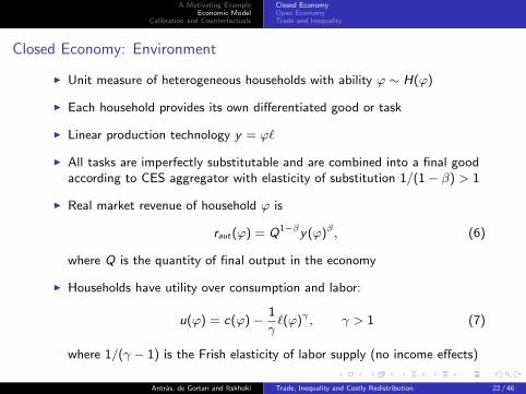
Closed Economy: Environment

I Unit measure of heterogeneous households with ability ϕ ∼ H(ϕ)

I Each household provides its own differentiated good or task

I Linear production technology y = ϕ`

I All tasks are imperfectly substitutable and are combined into a final goodaccording to CES aggregator with elasticity of substitution 1/(1− β) > 1

I Real market revenue of household ϕ is

raut(ϕ) = Q1−βy(ϕ)β , (6)

where Q is the quantity of final output in the economy

I Households have utility over consumption and labor:

u(ϕ) = c(ϕ)− 1

γ`(ϕ)γ , γ > 1 (7)

where 1/(γ − 1) is the Frish elasticity of labor supply (no income effects)





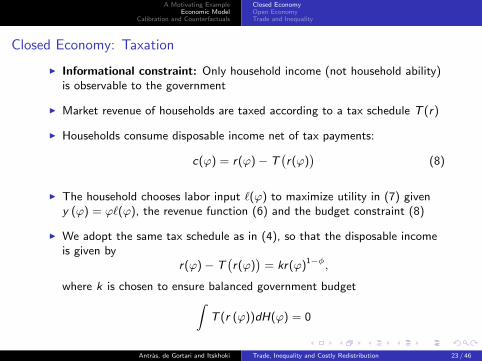
Closed Economy: Taxation

I Informational constraint: Only household income (not household ability)is observable to the government

I Market revenue of households are taxed according to a tax schedule T (r)

I Households consume disposable income net of tax payments:

c(ϕ) = r(ϕ)− T(r(ϕ)

)(8)

I The household chooses labor input `(ϕ) to maximize utility in (7) giveny (ϕ) = ϕ`(ϕ), the revenue function (6) and the budget constraint (8)

I We adopt the same tax schedule as in (4), so that the disposable incomeis given by

r(ϕ)− T(r(ϕ)

)= kr(ϕ)1−φ,

where k is chosen to ensure balanced government budget∫T (r (ϕ))dH(ϕ) = 0





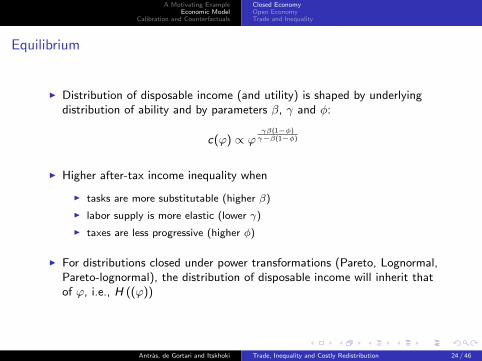
Equilibrium

I Distribution of disposable income (and utility) is shaped by underlyingdistribution of ability and by parameters β, γ and φ:

c(ϕ) ∝ ϕγβ(1−φ)

γ−β(1−φ)

I Higher after-tax income inequality when

I tasks are more substitutable (higher β)

I labor supply is more elastic (lower γ)

I taxes are less progressive (higher φ)

I For distributions closed under power transformations (Pareto, Lognormal,Pareto-lognormal), the distribution of disposable income will inherit thatof ϕ, i.e., H ((ϕ))





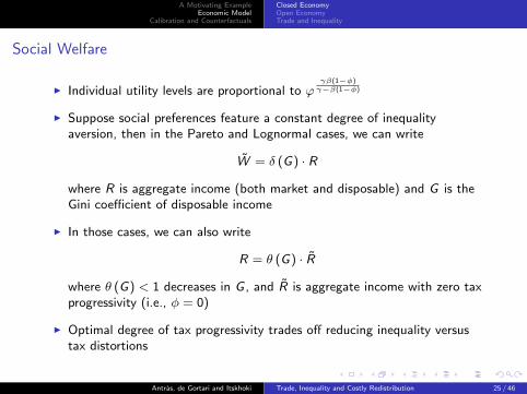
Social Welfare

I Individual utility levels are proportional to ϕγβ(1−φ)

γ−β(1−φ)

I Suppose social preferences feature a constant degree of inequalityaversion, then in the Pareto and Lognormal cases, we can write

W = δ (G) · R

where R is aggregate income (both market and disposable) and G is theGini coefficient of disposable income

I In those cases, we can also write

R = θ (G) · R

where θ (G) < 1 decreases in G , and R is aggregate income with zero taxprogressivity (i.e., φ = 0)

I Optimal degree of tax progressivity trades off reducing inequality versustax distortions





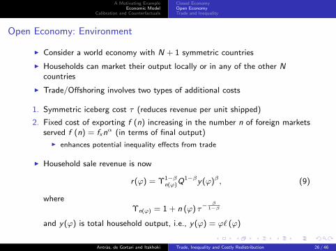
Open Economy: Environment

I Consider a world economy with N + 1 symmetric countries

I Households can market their output locally or in any of the other Ncountries

I Trade/Offshoring involves two types of additional costs

1. Symmetric iceberg cost τ (reduces revenue per unit shipped)

2. Fixed cost of exporting f (n) increasing in the number n of foreign marketsserved f (n) = fxn

α (in terms of final output)

I enhances potential inequality effects from trade

I Household sale revenue is now

r(ϕ) = Υ1−βn(ϕ)Q

1−βy(ϕ)β , (9)

whereΥn(ϕ) = 1 + n (ϕ) τ−

β1−β

and y(ϕ) is total household output, i.e., y(ϕ) = ϕ` (ϕ)





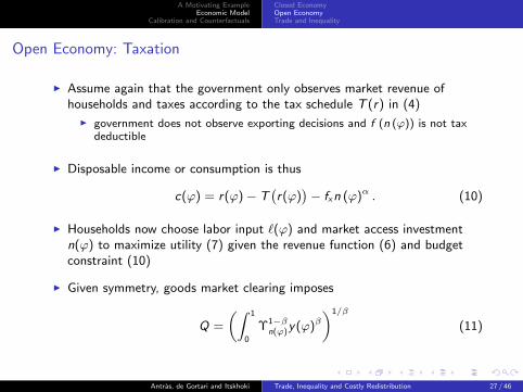
Open Economy: Taxation

I Assume again that the government only observes market revenue ofhouseholds and taxes according to the tax schedule T (r) in (4)

I government does not observe exporting decisions and f (n (ϕ)) is not taxdeductible

I Disposable income or consumption is thus

c(ϕ) = r(ϕ)− T(r(ϕ)

)− fxn (ϕ)α . (10)

I Households now choose labor input `(ϕ) and market access investmentn(ϕ) to maximize utility (7) given the revenue function (6) and budgetconstraint (10)

I Given symmetry, goods market clearing imposes

Q =

(∫ 1

0

Υ1−βn(ϕ)y(ϕ)β

)1/β

(11)





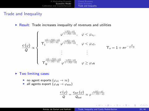
Trade and Inequality

I Result: Trade increases inequality of revenues and utilities

c (ϕ)

Q∝

ϕγβ(1−φ)

γ−β(1−φ) , ϕ < ϕx1 ,

Υγ(1−β)(1−φ)γ−β(1−φ)

1 ϕγβ(1−φ)

γ−β(1−φ) , ϕ < ϕx2,

......

Υγ(1−β)(1−φ)γ−β(1−φ)

N ϕγβ(1−φ)

γ−β(1−φ) ϕ ≥ ϕxN

Υn = 1 + nτ−β

1−β

I Two limiting cases:

I no agent exports (ϕx1 →∞)I all agents export (ϕxN → ϕmin)

c (ϕ)

Q=

caut (ϕ)

Qaut∝ ϕ

γβ(1−φ)γ−β(1−φ)





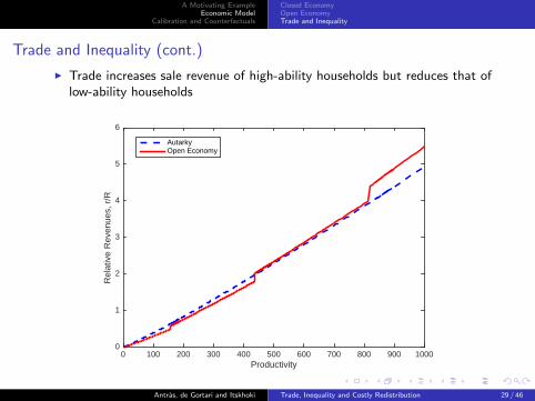
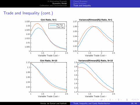
Trade and Inequality (cont.)

I Trade increases sale revenue of high-ability households but reduces that oflow-ability households

Productivity0 100 200 300 400 500 600 700 800 900 1000

Rel

ativ

e R

even

ues,

r/R

0

1

2

3

4

5

6

AutarkyOpen Economy





Trade and Inequality (cont.)

Variable Trade Cost =1 1.5 2 2.5

1

1.02

1.04

1.06

1.08

1.1

1.12Gini Ratio, N=10


1.2

1.3

1.4

1.5

1.6

1.7

1.8

1.9Variance(R/mean(R)) Ratio, N=10


1

1.005

1.01

1.015

1.02

1.025

1.03

1.035Gini Ratio, N=1

Pre-TaxPost-Tax


1.01

1.02

1.03

1.04

1.05

1.06

1.07Variance(R/mean(R)) Ratio, N=1





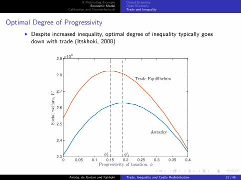
Optimal Degree of Progressivity

I Despite increased inequality, optimal degree of inequality typically goesdown with trade (Itskhoki, 2008)

Progressivity of taxation, φ0 0.05 0.1 0.15 0.2 0.25 0.3 0.35 0.4

Socialwelfare,W

×104

2.3

2.4

2.5

2.6

2.7

2.8

2.9

Autarky

Trade Equilibrium

φ∗

Tφ∗

A




CalibrationCalibrated Welfarist CorrectionCalibrated Costly Redistribution Correction

Calibration and Counterfactuals: Road Map

I We first calibrate the model to 2007 U.S. data (trade share, incomedistribution, tax progressivity)

I We then explore the implication of a move to autarky on

1. Aggregate Income

2. Income Inequality

I We use the model to gauge the quantitative importance of the twocorrections developed above

1. How large are the gains from trade for different degrees of inequalityaversion?

2. How large would the gains from trade be in the absence of costlyredistribution (i.e., φ = 0)?





Calibration

I Hold the following parameters fixed

1. Elasticity of substitution = 4 (β = 3/4)

I BEJK (2003), Broda and Weinstein (2006), Antras, Fort and Tintelnot (2014)

2. Iceberg trade costs (τ = 1.83)

I Melitz and Redding (2014), Anderson and Van Wincoop (2004)

3. Number of countries (N = 10)

I U.S. roughly 15% of world manufacturing output; results not too sensitive to Nabove 5

I Set baseline fixed cost fx to match a U.S. trade share of 0.14

I Set convexity of fixed costs to either α = 1 or α = 3 (consistent withpreliminary estimates exploiting cross-section of U.S. exports)

I Labor supply elasticity: experiment with various values for γ betweenγ = 10000 (or ε ' 0) and γ = 5/3 (or ε = 1.5)

I hotly debated parameter in the literature





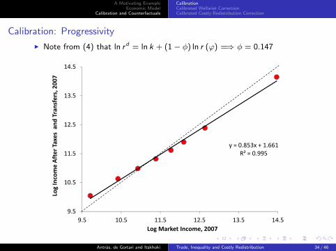
Calibration: Progressivity

I Note from (4) that ln rd = ln k + (1− φ) ln r (ϕ) =⇒ φ = 0.147

y = 0.853x + 1.661R² = 0.995

9.5

10.5

11.5

12.5

13.5

14.5

9.5 10.5 11.5 12.5 13.5 14.5

Log Income After Taxes and

Transfers, 200

7

Log Market Income, 2007





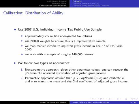
Calibration: Distribution of Ability

I Use 2007 U.S. Individual Income Tax Public Use Sample

I approximately 2.5 million anonymized tax returns

I use NBER weights to ensure this is a representative sample

I we map market income to adjusted gross income in line 37 of IRS Form1040

I we work with a sample of roughly 140,000 returns

I We follow two types of approaches:

1. Nonparametric approach: given other parameter values, one can recover theϕ’s from the observed distribution of adjusted gross income

2. Parametric approach: assume that ϕ ∼ LogNormal(µ, σ) and calibrate µand σ to match the mean and the Gini coefficient of adjusted gross income





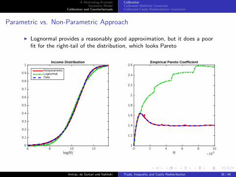
Parametric vs. Non-Parametric Approach

I Lognormal provides a reasonably good approximation, but it does a poorfit for the right-tail of the distribution, which looks Pareto

log(R)6 8 10 12

0

0.1

0.2

0.3

0.4

0.5

0.6

0.7

0.8

0.9

1Income Distribution

NonparametricLognormalData

R #1050 2 4 6 8 10

1

1.2

1.4

1.6

1.8

2

2.2

2.4

2.6Empirical Pareto Coefficient





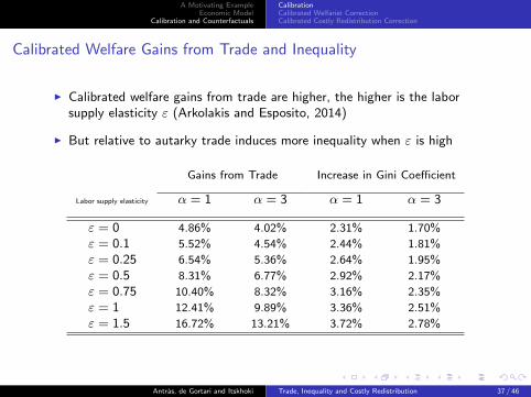
Calibrated Welfare Gains from Trade and Inequality

I Calibrated welfare gains from trade are higher, the higher is the laborsupply elasticity ε (Arkolakis and Esposito, 2014)

I But relative to autarky trade induces more inequality when ε is high

Gains from Trade Increase in Gini Coefficient

Labor supply elasticity α = 1 α = 3 α = 1 α = 3

ε = 0 4.86% 4.02% 2.31% 1.70%

ε = 0.1 5.52% 4.54% 2.44% 1.81%

ε = 0.25 6.54% 5.36% 2.64% 1.95%

ε = 0.5 8.31% 6.77% 2.92% 2.17%

ε = 0.75 10.40% 8.32% 3.16% 2.35%

ε = 1 12.41% 9.89% 3.36% 2.51%

ε = 1.5 16.72% 13.21% 3.72% 2.78%





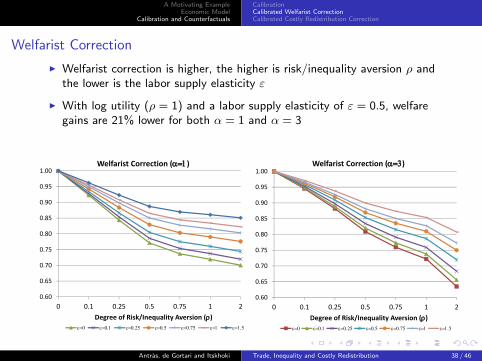
Welfarist Correction

I Welfarist correction is higher, the higher is risk/inequality aversion ρ andthe lower is the labor supply elasticity ε

I With log utility (ρ = 1) and a labor supply elasticity of ε = 0.5, welfaregains are 21% lower for both α = 1 and α = 3

0.60

0.65

0.70

0.75

0.80

0.85

0.90

0.95

1.00

0 0.1 0.25 0.5 0.75 1 2Degree of Risk/Inequality Aversion ()

Welfarist Correction ()

0.60

0.65

0.70

0.75

0.80

0.85

0.90

0.95

1.00

0 0.1 0.25 0.5 0.75 1 2Degree of Risk/Inequality Aversion ()

Welfarist Correction ()





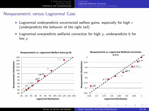
Nonparametric versus Lognormal Case

I Lognormal underpredicts uncorrected welfare gains, especially for high ε(underpredicts the behavior of the right tail)

I Lognormal overpredicts welfarist correction for high ρ, underpredicts it forlow ρ

0.65

0.7

0.75

0.8

0.85

0.9

0.95

1

0.65 0.7 0.75 0.8 0.85 0.9 0.95 1

Non

parametric

Distribution

Lognormal Distribution

Nonparametric vs. Lognormal Welfarist Correction(=0.5)

3%

4%

5%

6%

7%

8%

9%

10%

11%

12%

13%

14%

3% 4% 5% 6% 7% 8% 9% 10% 11% 12% 13% 14%

Non

parametric

Distribution


Nonparametric vs. Lognormal Welfare Gains (=0)





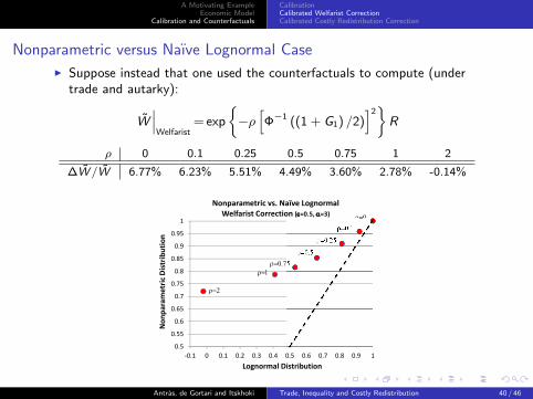
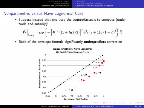
Nonparametric versus Naıve Lognormal Case

I Suppose instead that one used the counterfactuals to compute (undertrade and autarky):

W∣∣∣

Welfarist= exp

{−ρ[Φ−1 ((1 + G1) /2)

]2}R

ρ 0 0.1 0.25 0.5 0.75 1 2

∆W /W 6.77% 6.23% 5.51% 4.49% 3.60% 2.78% -0.14%

0.5

0.55

0.6

0.65

0.7

0.75

0.8

0.85

0.9

0.95

1

‐0.1 0 0.1 0.2 0.3 0.4 0.5 0.6 0.7 0.8 0.9 1

Nonparam

etric Distribution


Nonparametric vs. Naïve Lognormal Welfarist Correction (=0.5, =3)





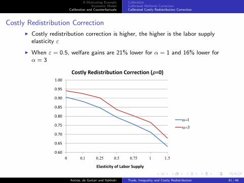
Costly Redistribution Correction

I Costly redistribution correction is higher, the higher is the labor supplyelasticity ε

I When ε = 0.5, welfare gains are 21% lower for α = 1 and 16% lower forα = 3

0.60

0.65

0.70

0.75

0.80

0.85

0.90

0.95

1.00

Elasticity of Labor Supply

Costly Redistribution Correction ( =0)





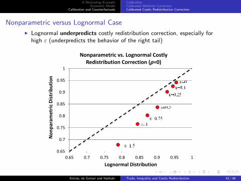
Nonparametric versus Lognormal Case

I Lognormal underpredicts costly redistribution correction, especially forhigh ε (underpredicts the behavior of the right tail)

0.65

0.7

0.75

0.8

0.85

0.9

0.95

1

0.65 0.7 0.75 0.8 0.85 0.9 0.95 1

Nonparam

etric Distribution


Nonparametric vs. Lognormal Costly Redistribution Correction ( =0)





Nonparametric versus Nave Lognormal CaseI Suppose instead that one used the counterfactuals to compute (under

trade and autarky):

W∣∣∣

Costly= exp

{−[Φ−1 ((1 + G1) /2)

]2

φ2ε (ε+ 1) / (1− φ)2

}R

I Back-of-the-envelope formula significantly underpredicts correction

0.65

0.7

0.75

0.8

0.85

0.9

0.95

1

0.65 0.7 0.75 0.8 0.85 0.9 0.95 1

Nonparam

etric Distribution


Nonparametric vs. Naïve Lognormal Welfarist Correction (=0.5, =3)





Corrections Do Not Compund

I Assume ε = 0.5 and α = 3 so both corrections reduce welfare gains by21%

I Does this imply an overall reduction of 37.6% (= 1− 0.792) in the welfaregains?

I Not if one evaluates the welfare gains under the same social welfarefunction (same ρ)!

I For ρ = 0, the overall correction is clearly 21%

I For ρ > 0, the welfarist correction kicks in, but the costly redistributioncorrection is diminished

I An inequality averse social planner is more likely to tolerate costlyredistribution to compensate for trade-induced inequality

I For high enough ρ, ‘welfarist’ gains from trade strictly higher with costlyredistribution than without it





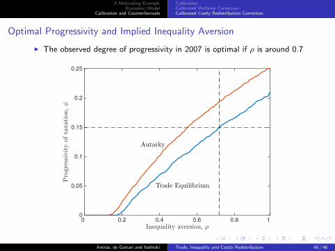
Optimal Progressivity and Implied Inequality Aversion

I The observed degree of progressivity in 2007 is optimal if ρ is around 0.7

Inequality aversion, ρ0 0.2 0.4 0.6 0.8 1

Progressivityoftaxation,φ

0

0.05

0.1

0.15

0.2

0.25

Trade Equilibrium

Autarky





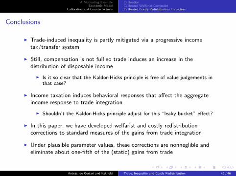
Conclusions

I Trade-induced inequality is partly mitigated via a progressive incometax/transfer system

I Still, compensation is not full so trade induces an increase in thedistribution of disposable income

I Is it so clear that the Kaldor-Hicks principle is free of value judgements inthat case?

I Income taxation induces behavioral responses that affect the aggregateincome response to trade integration

I Shouldn’t the Kaldor-Hicks principle adjust for this “leaky bucket” effect?

I In this paper, we have developed welfarist and costly redistributioncorrections to standard measures of the gains from trade integration

I Under plausible parameter values, these corrections are nonneglible andeliminate about one-fifth of the (static) gains from trade


Documents

Trade, Inequality and Costly Redistributionitskhoki/papers/TradeInequalityRedistribution... · A Motivating Example Economic Model Calibration and Counterfactuals Trade, Inequality