TRADE FLOWS USING TEXAS 254 COUNTIES DATA SETS

Hyunkyung JungGIS Term Project

November 29th, 2001

INTRODUCTIONS

Modeling long-run transportation demands

has been developed for Effect of the interactions between activities in

regional economies Daily Movement of Persons and Goods

which can be estimated by interaction between transportation and land use

INTRODUCTIONS

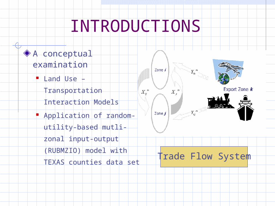
A conceptual examination

Land Use –

Transportation Interaction

Models

Application of random-

utility-based mutli-zonal

input-output (RUBMZIO)

model with TEXAS

counties data set

Trade Flow System

DATA COLLECTIONS

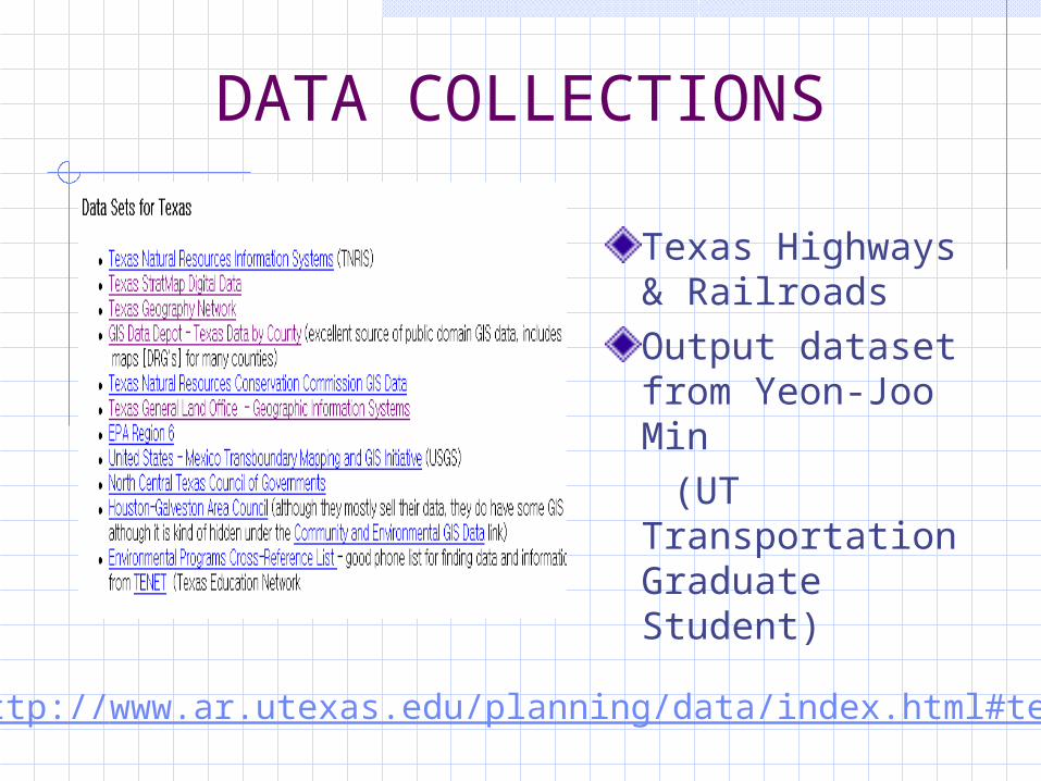
Texas Highways & RailroadsOutput dataset from Yeon-Joo Min

(UT Transportation Graduate Student)

http://www.ar.utexas.edu/planning/data/index.html#texas

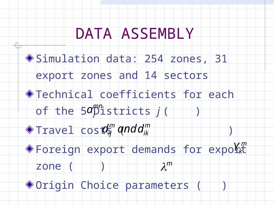
Simulation data: 254 zones, 31 export

zones and 14 sectors

Technical coefficients for each of the 5

Districts j ( )

Travel costs ( )

Foreign export demands for export zone

( )

Origin Choice parameters ( )

DATA ASSEMBLY

mnja

mkY

m

mik

mij dandd

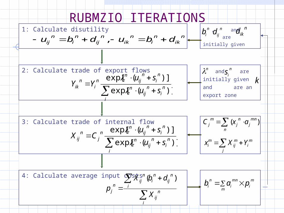
RUBMZIO ITERATIONS

4: Calculate average input costs

3: Calculate trade of internal flow

and are

initially given and

are an export

zone

2: Calculate trade of export flows

, and

are initially given

1: Calculate disutility n

ikni

nik

nij

ni

nij dbudbu ,

i

ni

nij

n

ni

nij

nnj

nij

su

suCX

)](exp[

)](exp[

i

nij

i

nij

ni

nij

nj

X

dbXp

)(

n

ib

n n

is

m

im

mn

i

n

i pab

nikd

n

ijd

k

i

ni

nij

n

ni

nij

nni

nik

su

suYY

)](exp[

)](exp[

n

mnj

nj

mj axC )(

mi

j

mij

mi YXx

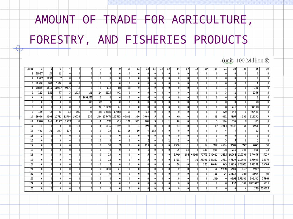
AMOUNT OF TRADE FOR AGRICULTURE,

FORESTRY, AND FISHERIES PRODUCTS

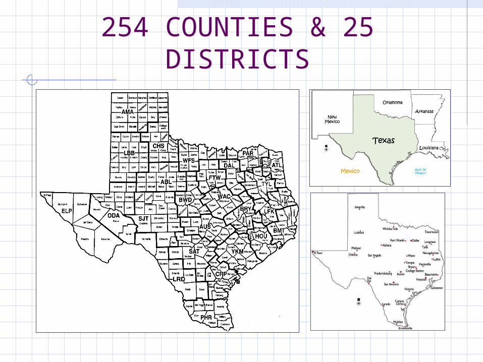
254 COUNTIES & 25 DISTRICTS

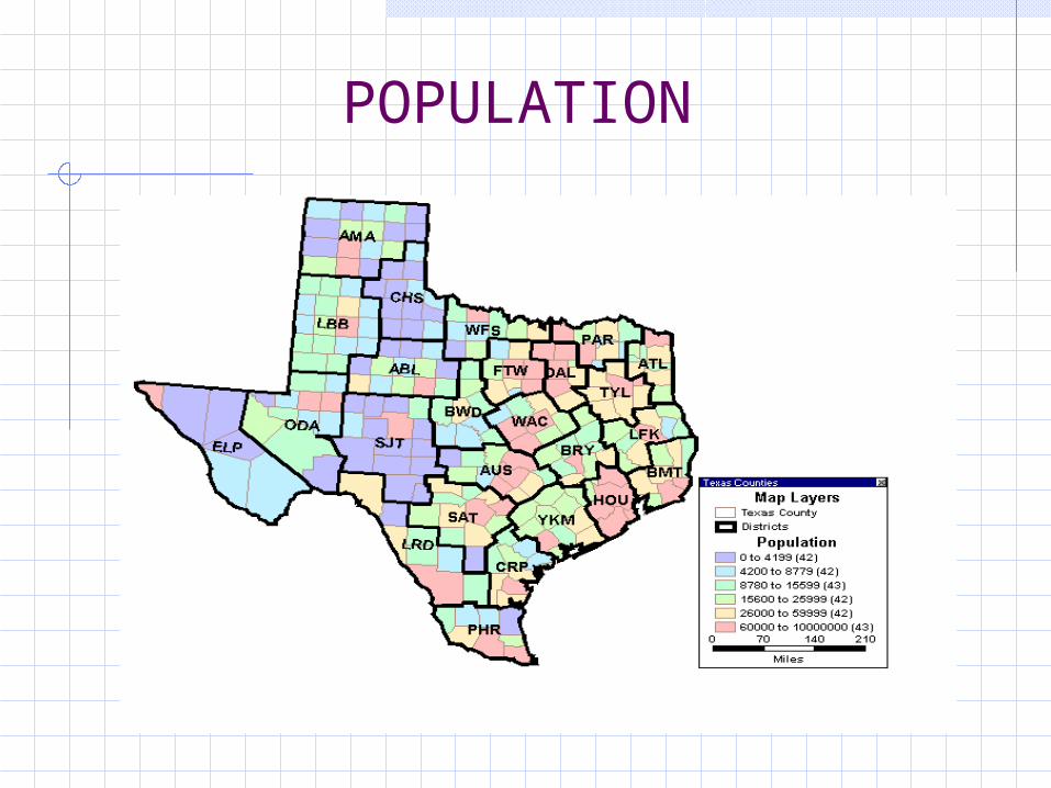
POPULATION

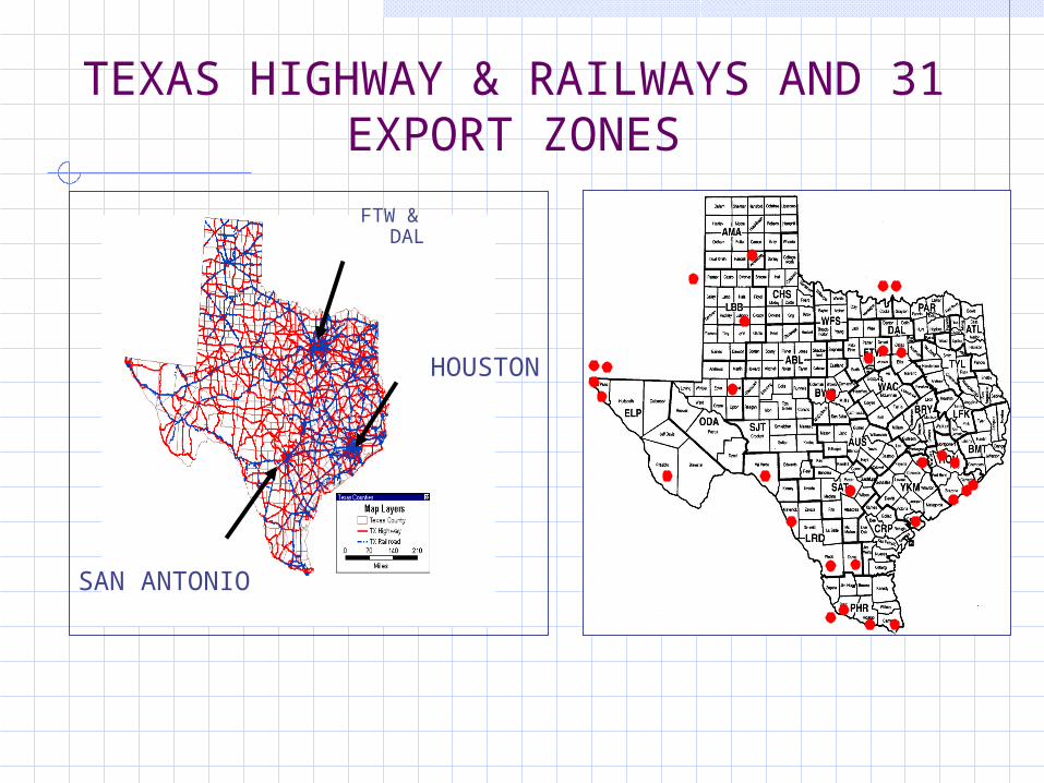
TEXAS HIGHWAY & RAILWAYS AND 31 EXPORT ZONES

HOUSTON

SAN ANTONIO

FTW & DAL

EMPIRICAL RESULTS

The amount of trade ( ) for each

sector is highly affected by the

transport costs/accessibility

Trade volumes in this example

highly favor the closest zones

mijX

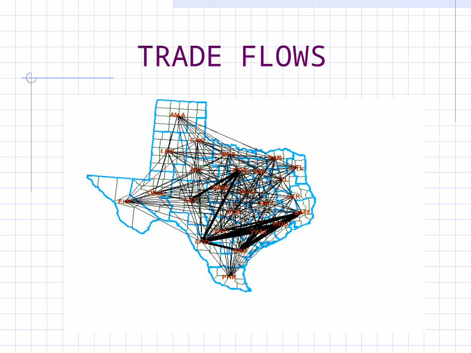
TRADE FLOWS

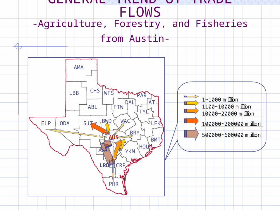
GENERAL TREND of TRADE FLOWS

-Agriculture, Forestry, and Fisheries from

Austin-

AMA

LBB CHS

ABL

WFS PARATL

TYL

DALFTW

ODA LFK

BRY

WACBWDSJTELP

PHR

CRP

BMTHOU

YKM

1~1000 million1100~10000 million10000~20000 million

100000~200000 million

500000~600000 millionAUS

SAT

LRD

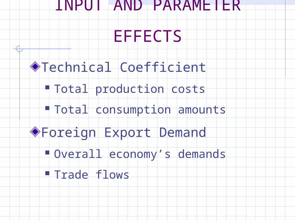
INPUT AND PARAMETER

EFFECTS

Technical Coefficient Total production costs

Total consumption amounts

Foreign Export Demand Overall economy’s demands

Trade flows

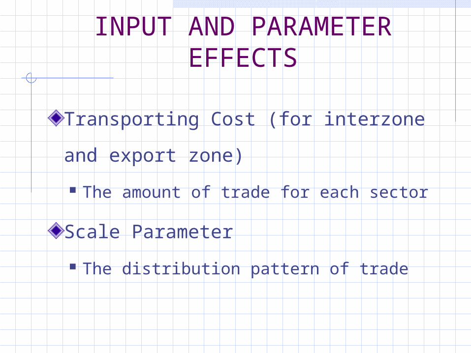
INPUT AND PARAMETER EFFECTS

Transporting Cost (for interzone

and export zone)

The amount of trade for each sector

Scale Parameter

The distribution pattern of trade

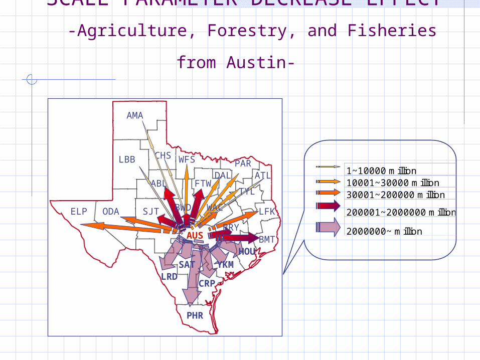
SCALE PARAMETER DECREASE EFFECT -Agriculture, Forestry, and Fisheries from

Austin-

AMA

LBB CHS

ABL

WFS PARATLDAL

FTW

ODA LFKELP

AUS

LRD

PHR

CRP

BMT

1~10000 million10001~30000 million30001~200000 million

200001~2000000 million

2000000~ million

TYL

SJT BWD

BRY

HOUSA

TYKM

WAC

CONCLUSIONS

Improvements to a zone’s technology significantly

enhanced its trade and production levels

Travel cost increases limited trade interactions, while

scale-parameter reductions increased interactions.

Increases in Export demands fed back through all

levels of the trading system, spurring demand and

trade flow increases everywhere.

CONCLUSIONS

RUBMZIO model

A valuable set of relationships to predict

trade flows, location choices/production

levels, and market prices

Assessing regional transportation, land

use, technology, and trade policies

FUTURE STUDY Represent trade-offs between supply and demand

and between transport costs and land values. 

Investigates the sensitivities of trade flows and other

model outputs to various inputs and parameters

Combine the mode choice parameter and origin

choice parameter and show the effect of each choice

on trade flow

Compare a variety of related land-use/transport

interaction models