DPRIETI Discussion Paper Series 10-E-007

Trade Creation and Diversion Effectsof Regional Trade Agreements on Commodity Trade

URATA ShujiroRIETI

OKABE MisaWakayama University

The Research Institute of Economy, Trade and Industryhttp://www.rieti.go.jp/en/

RIETI Discussion Paper Series 10-E-007

January 2010

Trade Creation and Diversion Effects of Regional Trade Agreements on Commodity Trade

Shujiro Urata* and Misa Okabe**

Abstract:

This paper examines the impacts of regional trade agreements (RTAs) on commodity trade, with a particular focus on trade creation and diversion effects. Based on the estimation of the gravity equation for commodity trade, dealing with zero-trade flow and endogeneity problems, we analyze the impacts of various types of RTAs involving 67 countries for 20 commodities during 1980-2006. We identify that partial scope (PS) RTAs and RTAs among developing countries tend to cause trade diversion. Taking tariff rates into consideration explicitly, our results suggest that trade diversion is likely to be caused by the remaining tariffs on imports from non-members, while trade creation would be caused by various factors besides the reduction in tariff rates. As for specific RTAs, the EU is shown to have a trade creation effect in trade of agricultural commodities, while the AFTA and the NAFTA have trade creation effects in all types of machinery trade. These results seem to indicate that regional production and distribution networks in machinery have been formulated thanks to the reduction of tariffs under RTAs. JEL classification: F10, F15 Keywords: RTA, FTA, gravity equation, zero-trade flows, commodity trade, trade creation effects, trade diversion effects * RIETI and the Graduate School of Asia-Pacific Studies, Waseda University. ** Economic Research Institute for ASEAN and East Asia and Faculty of Economics, Wakayama University. The authors are grateful for the comments received from Masahisa Fujita, Ryuhei Wakasugi, Katsuhide Takahashi, Mitsuyo Ando, Hirofumi Uchida, and Helen T. Naughton.

RIETI Discussion Papers Series aims at widely disseminating research results in the form of professional papers, thereby stimulating lively discussion. The views expressed in the papers are solely those of the author(s), and do not present those of the Research Institute of Economy, Trade and Industry.

1

1 Introduction According to the WTO, 421 regional trade agreements (RTAs) have been notified to the WTO since 1948

up to now, and 230 RTAs are in force1

In the light of the rapid expansion of RTAs, it is only natural that a large number of studies concerning the effect of RTAs on foreign trade have been carried out from both theoretical and empirical aspects. Of these studies, ex post evaluation of RTAs on trade flows plays a central role in empirical studies. Although the main object of these studies is to verify a very simple question, that is, whether RTAs have the trade creation and/or trade diversion effects, there seems to be little agreement as to the nature of the impacts of RTA on trade flows

. While the total number of notified RTAs is 124 for 36 years during 1948-1994, almost 300 additional RTAs have been notified for 13 years since 1995. Furthermore, it is projected that the number of RTAs runs to 400 by 2010.

2

Our analysis is based on the estimation of a gravity model, which has been applied extensively to explain the bilateral international trade flows for more than four decades. The pioneering studies in applying the gravity model to study international trade flows are Tinbergen (1962) and Poyhonen (1963), and since then numerous empirical analyses using the model have been conducted to provide various verifications on international trade. However, it was not until the late 1970s that theoretical foundation was developed. The first study that developed the theory is Anderson (1979), which derives a simple theoretical gravity equation from a framework of two countries under complete specialization. In the 1980s, ‘the new trade theory’ with an assumption of monopolistic competition that is used to explain intra-industry trade was applied to test the gravity equation

. There are two main unsettled issues on the estimation of the impacts of RTAs on trade. One issue

concerns the econometric methods used for the analysis. A number of studies estimated the gravity equation to find the impacts of RTAs. These studies have encountered econometric problems, such as endogeneity of RTA variables and treatment of zero trade flow values. Concerning the endogeneity problem, recent studies have applied econometric techniques such as instrumental variables (IV) method for cross-section data and fixed effect model or first differencing model for the panel data. Baier and Bergstrand (2007) argue that the most important source of endogeneity relationship is due to the omitted variable bias. The zero trade flow problem has attracted attention recently, and new estimation methods, rather than simply replacing zero by small values, have been attempted. We discuss this problem and we show how we deal with it in section 4.1.

The other issue is the level of analysis. Many studies examine the impacts of RTAs using aggregated trade data. However, such analysis does not seem to capture the impacts of RTAs, because generally the treatment of tariff reduction/elimination differs substantially by commodities. An appropriate analysis should examine the impacts of RTAs at commodity level.

In this paper we cope with these two types of unsettled issues. As for the endogeneity bias, we use panel data and include fixed effects to deal with unobserved heterogeneity of country-pairs. In addition, we apply the Heckman selection model to the gravity model to deal with the zero-trade flow problem. To overcome the problem caused by using aggregated trade data, we undertake the analysis by using commodity level trade data.

The structure of the paper is as follows. Section 2 briefly reviews the previous studies, which estimated effects of RTAs on trade by using the gravity model. Section 3 presents the theoretical framework and the specification of the gravity equation applied for the analysis. Section 4 discusses the estimation methodology and describes the data used for the analysis. Section 5 presents the results of estimation, while section 6 concludes and draws some policy implications. 2 Literature Review

3

1 As of December 2008. See WTO webpage, http://www.wto.org/english/tratop_e/region_e/region_e.htm 2 Baier and Bergstrand (2007) pointed out ‘fragility’ of estimated treatment effects of RTAs.

. Since the 1990s to date, a number of studies have tackled with econometric problems, which

3 For example, Helpman (1987) tested the hypotheses derived from the model by using cross-country and time series data, and Bergstrand (1989) developed the gravity equation based on monopolistic competition model. Baier and Bergstrand (2009) suggested a way to measure the price term in the gravity

2

were due to the characteristics of the gravity equation. In the context of the estimation of the effects of RTAs, one of the greatest concerns in this field is the

endogeneity of the explanatory variables. For example, Carrere (2006) dealt with this problem by applying instrumental variables method to panel data. Baier and Bergstrand (2007) suggested that first differential fixed effect model is effective to deal with the endogeneity problem. As they pointed out, the issue of endogeneity in the gravity equation is still unsettled and it should be delved in the future.

The main concern of this paper is to estimate the effects of bilateral and regional RTAs on commodity trade. Many studies applied the gravity equation to estimate the effect of RTAs on commodity or sectoral trade. Fukao, Okubo and Stern (2003) and Jayasinghe and Sarker (2008) estimated NAFTA’s trade creation and trade diversion effects by using commodity trade data. Although Fukao, Okubo and Stern estimated an equation based on a partial-equilibrium model under monopolistic competition by fixed effect model, endogeneity, multilateral price term and zero trade flows are not controlled explicitly. Gilbert, Scollay, and Bora (2004) used sectoral trade data to estimate the impacts of major regional RTAs, and Endoh (2005) analyzed disaggregated commodity-level trade data to verify the effect of the global system of trade preferences (GSTP). Similarly to the earlier studies, they did not adequately deal with the problems of endogeneity and zero-trade flows. Powers (2007) is one of few studies, which have attempted to remove biases caused by endogeneity and zero-trade flows by applying the first-differencing fixed effect model to the theoretically-consistent gravity model for sectoral trade data. He used panel data with 75 countries and 3 periods during 1990-2000 for ISIC 3-digit level 25 sectors. His estimated gravity equation is consistent with the theory, and controls biases to some extent. However, these results may suffer from the lack of robustness because the sample size on the time-series dimension is limited to only three periods with the intervals of five years4

{ }ikik EY ,

. In addition, the first-differencing fixed effects model omits time invariant variables such as distance between countries. These variables used as proxies of trade cost caused by transportation, non-tariff barriers and wholesale distribution have been shown to be significant by most studies.

While this paper adapts the specification of Powers (2007) and tries to deal with biases caused by endogeneity and zero-trade flows, we make full use of time-series data in order to capture the changes in trade flows particularly after the latter half of 1990s when the number of RTAs increased rapidly. 3. Application of the gravity equation to commodity trade flows 3.1 The Model

Similar to Powers (2007) who applied Anderson and van Wincoop (2004)’s “class of trade separable model” to his estimation with sectoral trade data, we also construct a gravity equation for commodity trade under the assumption of monopolistically competitive firms and two-stage budgeting that separates the allocation of expenditure across product classes (k = 1,…, K) from the allocation of expenditure within a product class across countries of origin (j = 1,…, J). In other words, “the class of trade separable” is grounded on the allocation of production and expenditure of country i to commodity k, is separable from the bilateral allocation of trade across countries, and the model is under the assumption of separable preferences and technology. The variety of commodity k has an identical aggregator across countries of origin, which takes the CES form with elasticity of substitution of commodity k expressed as kη . In addition to the identical aggregator of varieties across countries and the independence of trade cost from quantity of trade, the CES form of homothetic preference and the homogeneity equivalent for intermediate input demand simplify the demand equations and market clearing equations.

equation derived from the monopolistic competition model. 4 Estimated gravity equation in Powers (2007) includes average tariff rate as trade cost. Tariff rates are reported at intervals of several years generally, so that he constructs panel data covering 1990, 1995, and 2000.

3

The CES demand function for each variety in country i is derived as follows;

ikik

ijkijk E

Pp

xkη−

=

1

(1)

where ijkx is the demand of commodity k from country j by country i. ikP is the CES price index; kk

jijkik pP ηη −− ∑= 11 )()( (2)

ijkp is the import price, that is, c.i.f. price of country i’s import of commodity k shipped from country j. The

relation between c.i.f. price ijkp and its f.o.b. price in producer j, jkp is given by;

ijkjkijk Tpp = (3) where ijkT is the ad-valorem equivalent of trade cost of commodity k from country j to country i.

Solving the price jkp from the market clearing conditions ijkjki

ijkjkjk TpxYp ∑= and substitute the

result in (1) and (2), we can derive the gravity equation, in which country i’s import of commodity k from country depends on expenditure of commodity k country i, production of k by county j and the world production of commodity k, trade cost and price indexes interpreted as the multilateral resistance term, as follows:

k

jkik

ijk

Wk

jkikijk PP

TY

YEx

η−

=

1

(4)

where WkY is the world output of commodity k. 3.3 The estimation specification

Taking natural logarithms of both sides of equation (4) which is the gravity equation derived from the above theoretical framework, we obtain the following equation.

jkkikkijkkjkikkijk PPTYEYx ln)1(ln)1(ln)1(lnlnlnln ηηη −−−−−+++−= (5)

where ijkx is import value of commodity k from country j by country i, ikE is expenditure of commodity k

in country i and kY and jkY are production of commodity k in the world and in country j, respectively, ijkT is the trade cost affecting import directly when country i imports commodity k from country j. Following a number of studies using the gravity model to estimate RTA’s impacts, we assume that the bilateral trade cost is expressed as the following linear combination of observable measures.

]exp[ ijRTAijkLijkBijkijk RTALANBORDIST δδδλ −−−= (6)

where ijkDIS is the geographical distance between the largest cities of countries i and j measured by

kilometer, ijkBOR and ijkLAN are dummy variables that take unity if country i and j share a common

border and common official languages, respectively, and ijRTA is a RTA dummy variable that takes unity if

4

the country pair belongs to the same RTA. In our analysis of the impacts of RTAs on trade, we classify RTAs into three groups based on the following characteristics, the form of agreement, the number of members, and the level of economic development of the members. Besides, we examine the effects of seven major RTAs, that is, the European Union (EU), North American FTA (NAFTA), ASEAN FTA (AFTA), Mercado Comun del Sur (MERCOSUR), Andean Sub-regional Integration Agreement (CAN), Common Market for Eastern and Southern Africa (COMESA) and Pan-Arab FTA in order to verify differences in the impacts among different RTAs. Regarding the effects of RTAs on trade cost, two types of dummy variables are adopted, i.e., the first dummy equals unity if both the importer and the exporter belong to the same RTA, and the second dummy equals unity if the importer is a member of the RTA but the exporter is not a member. These RTA dummies are used to examine the trade creation and diversion effects.

Substituting equation (6) into equation (5), the estimation equation of commodity k is derived as (7)5

ijijijijij

jijiij

RTALANBORDISYYx

εβββββββαα

+++++

++++=

6543

210

ln

lnlnln

:

(7)

where 0β is a constant, which includes the world output, and,

RTA6L5B43 )1()1()1(,)1( δηβδηβδηβληβ −−=−−=−−=−= , We substitute commodity expenditure iE by iY and use real GDP of country i, and also use real GDP of country j in place of production of commodity k in country j,

jY . Although we should use expenditure and production data, there is no complete dataset on commodity production and expenditure data at such detailed level for all country so far. As for the price index, in the same way as Feenstra, we apply importer and exporter fixed effects. iα and jα are importer’s and exporter’s dummies, which control for Pik and Pjk respectively to avoid the omitted variables bias.6

4. Estimation method and data description

We also add year specific dummies to capture temporary factors such as global business cycles and global shocks.

4.1 Econometrical method

The estimation of the gravity equation is subject to several econometric problems. According to Baier and Bergstrand (2007), explanatory variables of the gravity equation including RTA terms tend to be correlated with the error term ijkε , namely the problem of endogenous biases. They pointed out the possibility of endogenous bias caused by characteristics of RTA, omitted variables and simultaneity bias. The omitted variables problem comes from the correlation between the decision to form an RTA and unobservable bilateral economic or policy related conditions included in the error term. Baier and Bergstrand (2004) showed empirical evidence that a probability of the formation of a RTA between two countries is higher the larger GDP and more similar economically are the two countries. The probability of an FTA is also higher the larger the difference between two countries relative factor endowments. These factors are regarded to bring the potential trade creation and urge the governments to from the RTAs, but they are not included obviously in the gravity model.

Baier and Bergstrand (2007) pointed out that instrumental variables (IV) method applied to cross-section data so as to address the endogenous bias are not reliable because of difficulties of selection of proper IVs. Instead of using IVs they suggested an application of the fixed effects model by using panel data because the source of the endogenous bias in the gravity equation could be unobserved time-invariant heterogeneity.

5 Subscript k is omitted here for simplicity. 6 The other typical way to replace price index term is to construct ‘multilateral resistance term’ as a function of weighted average of trade cost with all importers and exporters (see Baier and Bergstrand (2009)).

5

Powers (2007) applied a fixed effects first-differenced gravity equation by using sectoral data to avoid the problems of serial correlation in error terms7

0~0

0~~ln

lnln~

6543

210

≤=

>=

+++++

++++=

ijtijt

ijtijtijt

ijtijtijijij

jtitjiijt

xifxxifxx

RTALANBORDISYYx

µγγγγγγγϕϕ

. While it is important to remove the serial correlation in error terms, the first differencing process has a

serious defect for estimation of the gravity equation on trade flows. It drops important time invariant variables such as bilateral distance and common language which are proxies for bilateral trade cost such as transportation cost and non-tariff barriers. These time invariant variables account for a large part of trade cost, and estimated coefficients of these variables are shown to be statistically significant and stable in the most studies estimating the gravity equation. Powers (2007) only used three time periods with five year intervals, namely 1990, 1995 and 2000, because of data availability. However, use of three data points rather than a time-series data raises possibility of sample selection bias when the selection of period is arbitrary and deleted samples have some common tendencies such that the country-pairs of developing countries tend to release a few trade flow data once in several years. Our main interest is to estimate the effect of RTAs on trade flows. Hence it is important to use annual data because the formation of RTAs increased rapidly every year after the latter half of 1990s.

Zero-trade flow problem is also a matter of serious concern for estimation of the gravity equation. In particular, zero-trade and zero-valued trade which are less than the reporting threshold appear frequently in sectoral and commodity trade data. For instance, the percentage of zero-trade flows in total number of our sample is 49%. Most studies on RTA effect by estimating gravity equation have omitted zero-trade flows since the log of zero value is not defined. However, omitting zero-trade flows results in biased result if zero-trade flows do not occur randomly. It seems appropriate to regard that some factors such as long distance, lack of political and cultural links, and large difference in production structures cause zero-trade between countries.

Several studies dealt with zero-trade flows by using the Tobit model (e.g. Soloaga and Winters (2001)), Pseudo Poisson maximum likelihood method (e.g. Tenreyro (2007) and Komorovska, Kuiper and Tongeren (2007)) and Heckman sample selection model (e.g. Linders and Groot (2006)). Marin and Pham (2008) investigate these estimators with data generated using a heteroacedastic and limited-dependent-variable process by Monte Carlo simulations. They demonstrated that Pseudo Poisson Maximum Likelihood estimator yields severely biased estimates when zero trade flows are frequent. Linders and Groot (2006) investigated Tobit model and Heckman sample selection model approaches, and concluded that Heckman sample selection model takes into account the information provided by zero-valued observation more correctly. On the ground that zero-trade flows are the result of firm’s decision making based on potential profitability of trade, we also adopt Heckman sample selection model. The sample selection model is specified as follows;

Selection equation:

(8)

Regression equation:

ijtijtijijij

jtitjiijt

RTALANBORDISYYx

εβββββββαα

+++++

++++=

6543

210

ln

lnlnln (9)

ρεµσεµ =),(r),0(N~),1,0(N~ 2 Where, xijt is an indicator for doing bilateral trade. µ and ε are unobserved disturbances, and r

denotes correlation coefficient. The selection equation determines whether or not bilateral trade are observed or not, and the regression equation determines amount of bilateral trade. These parameters are estimated using the method of maximum likelihood.

7 When Wooldridge (2002, 282–283)’s simple test for autocorrelation in panel-data are carried to a first-differenced gravity model using our dataset, the null hypothesis is not be rejected for all commodities.

6

4.2 Data The dataset used for our estimation is a panel data with 67 countries/regions and 27 years from 1980 to

2006 at 20 commodity level. For the purpose of removal of temporary contingent changes, we include time dummies.

Bilateral commodity trade data are taken from the World Integrated Trade Solution (WITS), which provides the data and information on trade, developed by the World Bank in collaboration with UNCTAD. The trade flow data provided by WITS are obtained from the United Nation’s Commodity Trade Statistic Database (COMTRADE). We use data at SITC 2 digit level to retain the largest available sample size. GDP data are from the World Bank’s World Development Indicators. Regarding GDP of Republic of China (Taiwan), we use GDP released by National Statistical Bureau of the Republic of China. Both commodity trade and GDP are converted into value in real US dollars by using exchange rates and the U.S. consumer price index from the Bureau of Economic Analysis. The information on BOR and LAN are obtained from ‘the regional basic data’ provided by the website of the Ministry of Foreign Affairs of Japan. DIS is the distance between the largest cities of country i and j measured by kilometer, which is calculated by latitude and longitude of each cities. RTA dummy variables are created based on the information on the year of establishment, which is available on the WTO website. Regarding the EU and AFTA dummies, the number of signatory countries has changed during the sample periods, thus these dummies do change reflecting on the new members. 4.3 Statistical description of the sample data

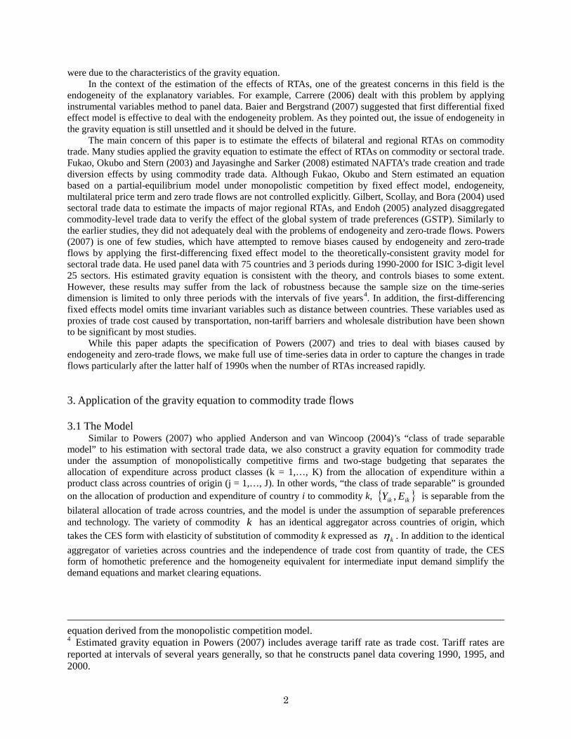
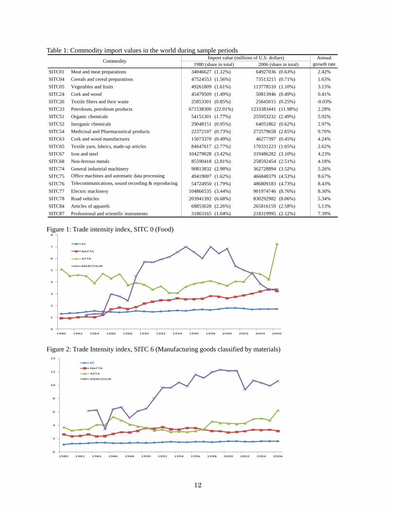
Before discussing the estimation results, we would like to make some observations on the sample data. We use commodity import values for dependence variable of the estimation. Table 1 shows import values of the world and its annual growth rate during the sample period for 20 commodities. Petroleum (SITC33), road vehicles (SITC78), electric machinery (SITC77) account for large shares of total imports. While total import value in the world increases from 0.16 trillion to 12 trillion at an annual growth rate of 7.5 percent, the growth rate in all machineries (SITC74, 75, 76 and 77) and medicinal products (SITC54) during the sample periods are high exceeding 8%. By contrast, import values of food (SITC01, 04, 05), Crude materials (SITC24, 26) and mineral fuels (SITC33) grew at lower rate, resulting in the decline in their share in total

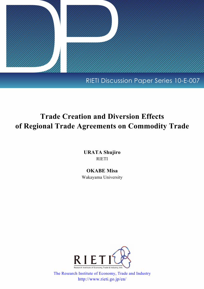
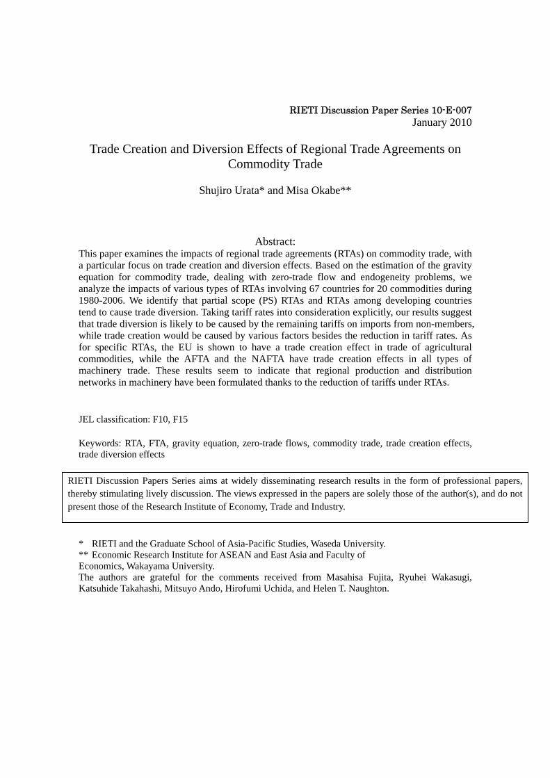
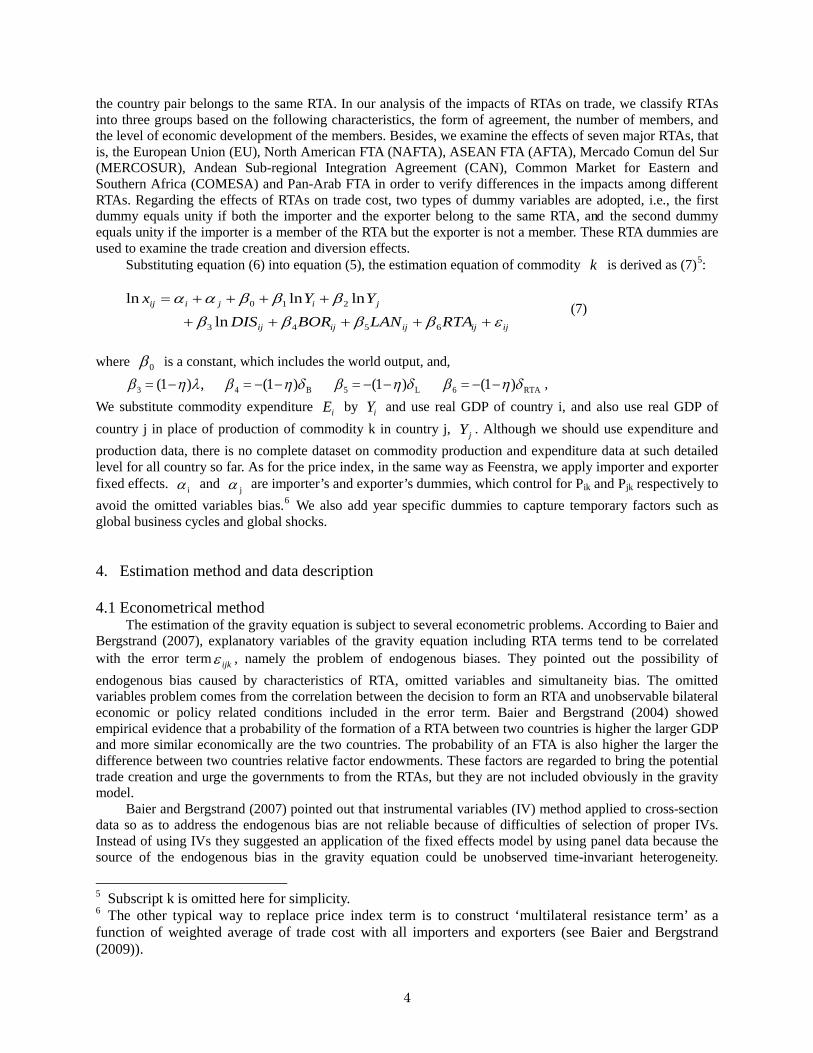
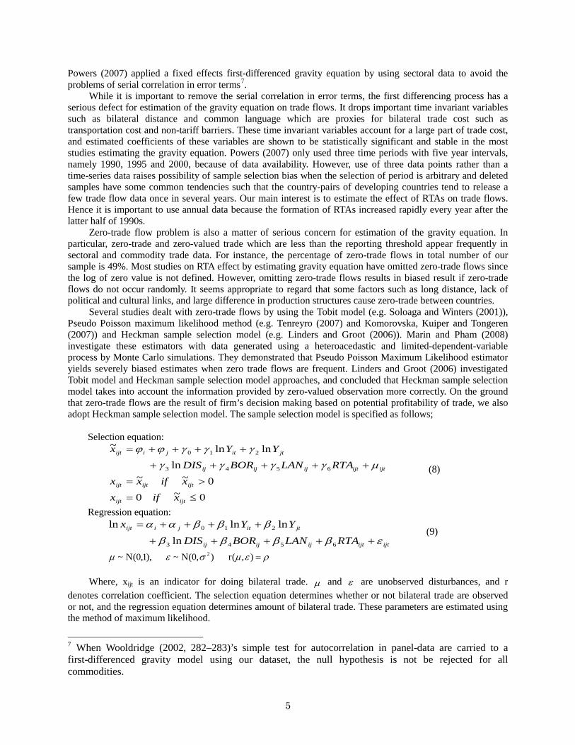
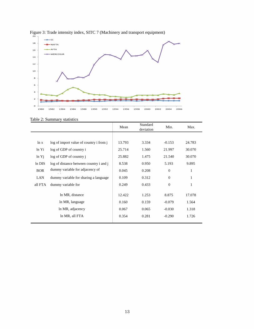
Turning our attention to regional trade, we make use of trade intensity index calculated by sample countries’ bilateral import and export values. Trade intensity index are calculated as a ratio of a share of intra-region trade in regional total trade and a share of regional total trade in the world trade, namely (Xii / Xiw) / (Xiw / Xww). Xii represents intra-region trade, Xiw region i’s trade with the rest of the world, and Xww world trade. Trade intensity index measures the degree of trade relationship. Trade relationship is more (less) intensive (or biased) than average if the value of trade intensity is greater (less) than unity. Trade intensity indexes in trade of food (SITC0), manufactured goods classified by materials (SITC 6) and machinery and transport equipment (SITC7) of EC, NAFTA, MERCOSUR and AFTA are shown in figure 1-3. MERCOSUR has seen a high index value from the 1990s to the beginning of 2000s in food, manufactured goods and machinery, however the value for food declines after 2000. AFTA has a high index values in 1980s in the three categories, and the value declined in the 1990s then increased after 2005. The index value of food trade in NAFTA increased, however the index values in manufactured goods and machinery did not change much during the periods. The index values for the EU are the lowest and unchanged during the sample periods. From the analysis of the regional trade intensity index, it appears difficult to discern the effects of RTAs on trade flows. Summary statistics of the variables used for the estimation are shown in Table 2. 5. Estimation Results 5.1 Results of a benchmark estimation

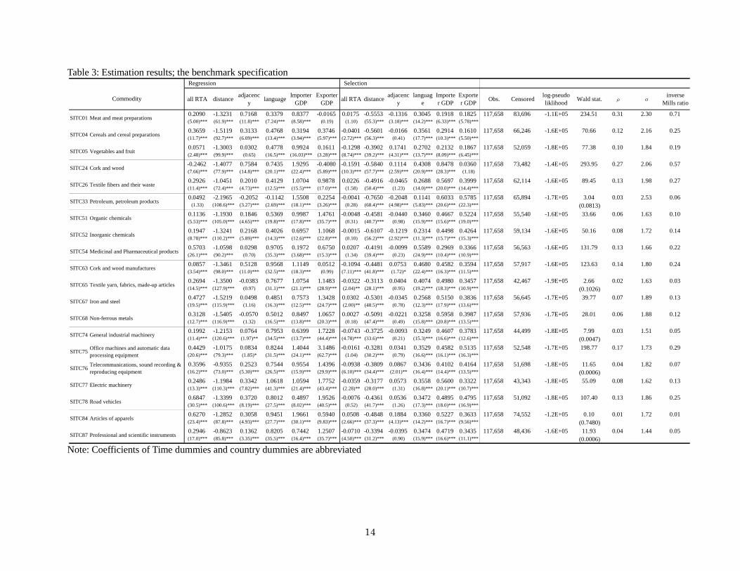
First, we estimate equations (12) and (13) with a RTA dummy variable, for the benchmarking purpose, using Heckman sample selection model. Table 3 shows the estimation results of equations (12) and (13). Taking a look at the estimation results of selection model, we find that country i and j's GDP, a common language, close distance between countries have an effect which causes firm in country i to start to import from

7

country j. Regarding the effect of RTA on decision to start import, there is no positive effects except for iron and steel and articles of apparels. Instead, significant and positive effects are found in the cases of nine commodities. These results imply that the decision to starts import or not depends on not RTA effect but importer's demand, exporter's production and trade cost determined by geographical and cultural distance between countries. Then, we focus on effects of RTA on existing commodity trade in this paper.

As for the estimated coefficients of regression equation (13), both coefficients of importer’s and exporter’s GDP are positive and statistically significant at the level of 1% in all the commodities except for importer’s GDP in the cases of meat and meat preparations (SITC01) and cork and wood (24). The estimated coefficient of exporter’s GDP tends to be large in the case of machinery trade, such as office machines (SITC75), and road vehicles (SITC78). Regarding the trade cost variables, the estimated coefficients of the distance are negative and statistically significant for all commodities and the coefficients of language shows positive significantly for all commodities except for petroleum (SITC33). The estimated results indicate that transportation cost and cultural similarity respectively proxied by distance and language dummies are important factors representing trade cost in commodity trade. By contrast, the signs of the estimated coefficients on adjacency, which are expected to be positive, are not uniform. The estimated coefficients are positive and statistically significant for 14 commodities out of 20 commodities.

The coefficient of the RTA dummy variable in the benchmarking estimation, namely “all RTAs,” denotes the impact of the RTA on imports from the member of the same RTA. The estimated coefficients for all commodities except for 2 commodities (SITC24 and 33) show positive signs at 1% level of significance. These results indicate that the trade creation effects of FTAs are found in 18 commodities. The estimated coefficients for ‘medicinal and pharmaceutical products (SITC54)’, ‘road vehicles (SITC78)’ and ‘articles of apparels (SITC84)’, are found relatively larger than for other commodities. Recognizing that the MNF tariff rates on articles of apparels and road vehicles are relatively high (Annex Table 3), one would suppose it reasonable to find significant trade creation effects by RTA for these commodities. Agricultural products (SITC 01, 04 and 05), by contrast, does not show large coefficients in spite of relative high tariff rate. This result may reflect the fact that many RTAs exclude agricultural products from tariff elimination because of their political sensitivity. 5.2 Trade creation and diversion effects by types of FTAs

Various types of RTAs can be identified, for example, in terms of the coverage of tariff elimination, the characteristics of member countries, and the number of member countries. The impacts of RTA on commodity trade are likely to be different for different types of RTAs. To examine the differences in the impacts by types of RTAs, we adopt the following three classifications. First, we apply the WTO’s classification by the form of agreement. Second, we divide all RTAs into bilateral and multilateral RTAs. The third is a classification according to the level of economic development of the RTA members, namely RTAs among developed countries, RTAs among developing countries, and RTAs between developed and developing countries. We construct two RTA dummies which capture trade creation and trade diversion effects for the three estimations. The RTA dummy variable which captures the trade creation effect is the same as the one used in the previous section, while the RTA dummy variable which captures the trade diversion effect equals unity when the importer country belongs to a RTA but the exporter country does not. If the coefficient is significantly negative, it denotes that import from non-member country deceases because of the formation of RTA.

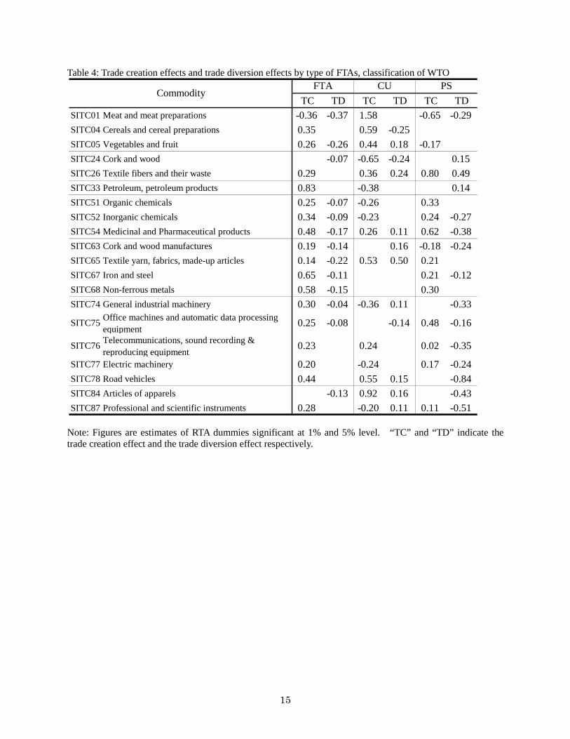
We first examine the impacts of RTAs on trade by classifying RTAs according to the WTO, namely, free trade agreement (FTA), customs union (CU) and partial scope agreement (PS)8

FTA is an agreement, under which the FTA members remove tariffs and other restrictions on trade between the members. As annex table 2 shows, among three types of RTAs, FTAs are the largest in number. CU is an agreement, under which not only tariffs and other restrictions on trade between the members are eliminated (i.e. FTA), but also the common external tariffs are applied to imports from non-members. Major CUs are EC, MERCOSUR and GCC. This agreement is the next largest to FTA. PS covers only certain products. Most of agreements classified into PS are agreements among developing countries, such as Global System of Trade Preferences among Developing Countries (GSTP), Economic Community of West African

.

8 Although the classification of the WTO, Economic Integration Agreement (EIA) also is included, we added EIA into FTA since our main concern is on commodity trade rather than trade of service.

8

States (ECOWAS) and ASEAN-China. Table 4 shows the summary of the estimation results of regression equation. The table extracts significant

estimated coefficients of RTA dummy variables at 1% and 5% significant levels for the regression equation of each commodity. Two types of RTA dummies, one to capture the trade creation effect (TC) and the other the trade diversion effect (TD), are adopted in the estimation. The result shows that FTAs give rise to both trade creation and trade diversion effects in many commodities, trade creation in 17 commodities and trade diversion in 13 commodities. The trade creation and diversion effects are found in a fewer number of commodities in the case of CU, trade creation in 9 commodities and trade diversion in 3 commodities. In the light of the characteristics of CU, it is reasonable to suppose that trade diversion effects are restrained due to establishment of common external tariffs, which are generally set equal to the lowest tariffs of the member countries.

Although partial scope (PS) has trade creation effect in more than a half of all commodities, it causes the trade diversion effects in 12 commodities. Substantial trade diversion effects found for PS seem to be attributable to high tariffs imposed by developing countries. When countries with very high tariffs form an RTA, their bilateral trade is likely to increase at the expense of their trade with non-members.

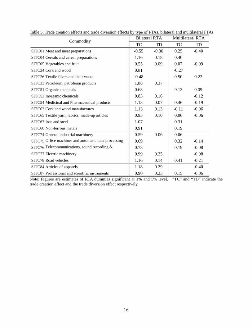
Next, we classify all RTAs into two types, namely, bilateral and multilateral RTAs. Table 5 shows the summary of the estimation results of the regression equation. Although bilateral RTAs are shown to have trade creation effects in almost all commodities except for meat (SITC01) and textile fibers (SITC26), trade diversion effects are caused only in meat (SITC01). In contrast, multilateral RTA also shown to have trade creation effect in 14 commodities, however it gives rise to trade diversion effects in more than a half of all commodities. These findings indicate that a bilateral RTA tends to be formed by a country pair which has much potentiality to increase bilateral trade while its impact on the rest of the world, namely trade diversion effect is relatively smaller than in the case of multilateral RTAs. This finding may reflect the fact that the scope for trade diversion is small when RTA membership is limited to two, and it gets larger with the number of FTA membership.

Lastly, we classify FTAs by member’s level of economic development. We divided sample countries into two groups, that is, countries which belong to the Group of 77 and the other. The former group of countries consists of developing countries, while the other group includes developed countries. It is possible to use the other indicators such as per capita GDP to measure the level of economic development. However, adoption of such indicator leads to a situation where the country composition of the groups changes. We construct four RTA dummies, that is, RTA among developed countries, RTA among developing countries, RTA between developed countries and developing countries. The RTA between developed countries and developing countries is divided into two cases, that is, one is that the importer is a developed country and exporter is a developing country, and the other case is the reverse.

Table 6 reports the summary of the estimation results of the regression equation. RTAs among developed countries cause the trade creation effect in almost all commodities except for cork and wood (SITC24) and organic chemicals (SITC51). The estimated coefficients in agricultural products (SITC01-05), materials (SITC63-68), telecommunication equipments (SITC76), electric machinery (SITC77), road vehicles (SITC78) and articles of apparels (SITC84) are larger compared with those for other RTAs. RTAs among developing countries bring about the trade creation effect in 12 commodities, while trade diversion effects are found in many commodities. These results are consistent with the earlier observation on the impacts of RTAs among developing countries, that is, partial scope (PS) RTA which includes many RTAs among developing countries.

Average tariff rates of developing countries are relatively high compared with average tariff rates of developed countries. Annex table 4 shows simple average tariff rate of the commodities during 1988-2006. The simple average tariff rate of G77 against all countries on agricultural product (SITC 01-05), textile yarn (SITC65), road vehicles (SITC78) and articles of apparels (SITC84) are about 20% and higher, and cork and wood manufactures (SITC63), telecommunications equipment (SITC76), electric machinery (SITC77) are also relatively high, and estimated coefficients of Trade diversion effect of these commodities are also relatively high. In light of these high tariff rates, it seems natural that trade diversion effects of RTAs involving only developing countries should be observed in many commodities, particularly in agricultural products, material products and machinery products as high tariff rates are applied to imports from non-member countries. Meanwhile, the relationship between trade creation effect and tariff rate are not so clear. In the case of RTAs

9

among developed countries, the estimated coefficients of trade creation are relatively large for both road vehicles (SITC78) and articles of apparels (SITC8), although tariff rates between developed countries on these products are different. This result suggests that trade creation effect could be caused by other factors, such as potential demand of importer and productivity of exporter, rather than just tariff elimination.

Regarding the case of RTAs between developed country importer and developing country exporter and in the reverse case, trade creation effects are found in about half of commodities, and trade diversion effects are less than the cases of RTA between developing countries. Estimated coefficient of trade diversion effect between developed country importer and developing country exporter in the case of apparels is larger than in other cases. Likewise, trade diversion effects between developing country importer and developed country exporter in road vehicles is the largest among all industries. Similar to the above results, the higher tariff rate remains on import from non-members, the larger trade diversion effect may occur.

5.3 Trade creation and diversion effects in specific RTAs In this section, we analyze the trade creation and diversion effects in seven multilateral RTAs, that is,

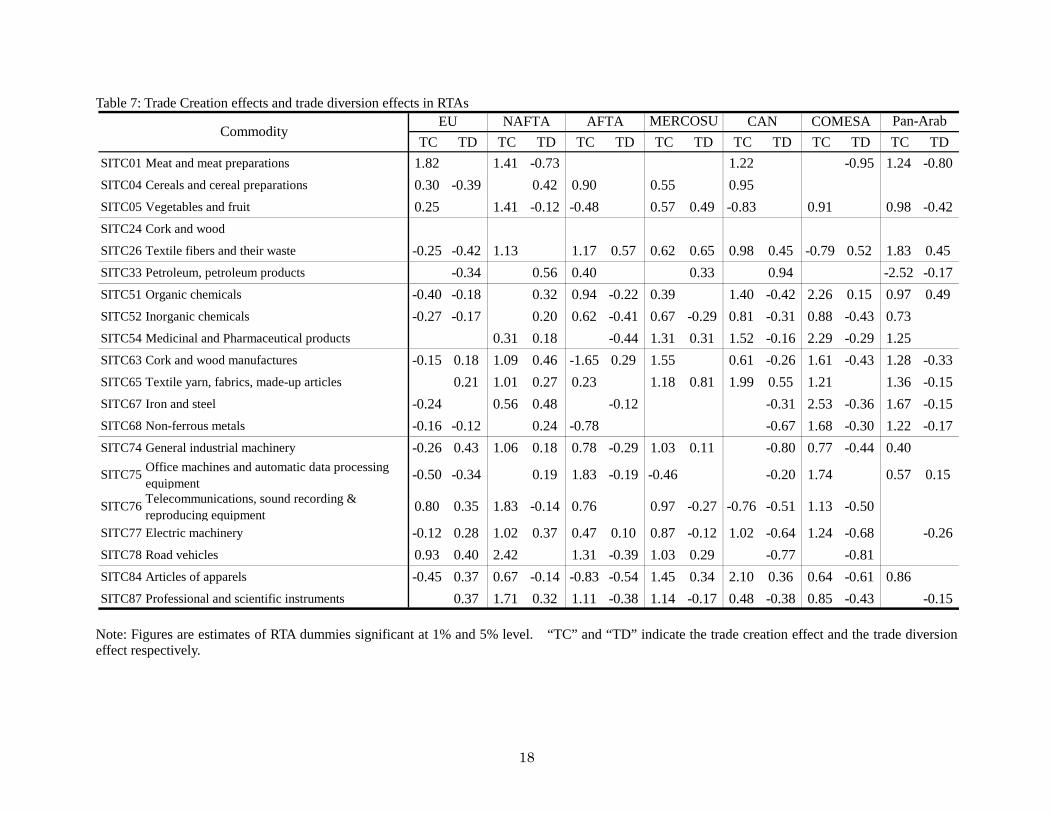
European Union (EU), North American FTA (NAFTA), ASEAN FTA (AFTA), Mercado Comun del Sur (MERCOSUR), Andean Sub-regional Integration Agreement (CAN), Common Market for Eastern and Southern Africa (COMESA) and Pan-Arab FTA. Table 7 shows the summary of the estimation results of the regression equation. Regarding the trade creation effects, all RTAs except for the EU led to the increase in trade among the members in more than a half of the commodities. While the EU has the trade creation effects in agricultural products trade, AFTA has trade creation effects in all types of machinery trade. NAFTA also has trade creation effects in almost all machinery products, in particular the estimated coefficient in road vehicles (SITC 78) is the largest among all RTAs. These findings appear to support a view that FTAs contribute to the formation of regional production networks, as regional production networks in machinery production have been created in ASEAN and NAFTA regions9

6 Conclusions

. Trade diversion effects vary among the RTAs under study. Trade diversion effect was detected in four

products each in the NAFTA and MERCOSUR. The number of products showing trade diversion is larger for the AFTA, CAN and COMESA. For the CAN and COMESA, the trade diversion effect and relative large coefficients are detected in almost all of material trade (SITC63-68) and machinery trade (SITC74-78), while for the AFTA trade diversion and relatively large coefficients are found in all chemical products (SITC51-54) and articles of apparels (SITC84). Taking account of the possibility that the trade diversion effect reduces economic welfare of the RTA members, the AFTA, CAN and COMESA countries are advised to lower their MFN (most-favored nation) tariff rates to minimize the trade diversion effect.

We analyzed the impacts of RTAs on commodity trade flows, with a particular focus on their trade creation and diversion effects, by estimating the gravity equation covering 67 countries/regions for 27 years from 1980 to 2006 at 20 commodity level. In our estimation, we dealt with the problems of endogeneity and zero trade flows, which had not been treated adequately in the previous analyses.

Recapitulating the major results, we found that the impacts of RTAs on trade flows differ by commodities and types of RTAs. We found that FTAs generate both trade creation and trade diversion effects in many commodities in the case of FTAs, while trade creation and diversion are found in fewer commodities in the case of CU. Moreover, we found that multilateral RTAs caused trade diversion in many more commodities compared to the case of bilateral RTAs. As to the characteristics of the members of RTAs, we observed that while RTAs among developed countries generate the trade creation effect in almost all commodities except for wood and organic chemicals, while the trade diversion effect was not found. In contrast, RTAs among developing countries have the trade creation effect in 12 commodities, while they give rise to the trade diversion effect in 16 commodities with respect to imports from developed countries. These results suggest that high tariffs imposed on imports from non-members by developing countries are a primary factor causing trade diversion. Similar findings on the impacts of the characteristics of RTA members are obtained from the 9 For regional production networks in East Asia, see, for example, Ando and Kimura (2009).

10

analysis of seven specific RTAs. One important policy implication from our empirical analysis is the need to lower tariff rates on imports

from non-RTA members. In other words, global trade liberalization under the WTO should be pursued by the WTO members. This policy implication comes from the observation that RTAs involving developing countries, which have higher tariffs than developed countries, lead to trade diversion in many commodities. References Anderson, J. E., 1979, “A Theoretical Foundation for the Gravity Equation”. American Economic Review,

69 (1), pp.106-116. Anderson, J. E., and Eric vanWincoop, 2003, “Gravity with Gravitas: A Solution to the Border Puzzle”,

American Economic Review, 93 (1), pp.170-192. Anderson, J. E., and Eric van Wincoop, 2004, “Trade Cost”, Journal of Economic Literature, 42 (3),

pp.691-751. Anderson, J. E., 2004, “Trade Costs”, Journal of Economic Literature, 42 (3), pp.691-751. Ando, M. and F. Kimura, 2009, Fragmentation in East Asia: Further Evidence, ERIA Discussion Paper

Series, ERIA-DP-2009-20, ERIA, Jakarta Baier, S. L., and J. H. Bergstrand, 2004, “On the Economic Determinants of Free Trade Agreements”,

Journal of International Economics, 64 (1), pp.691-751. Baier, S. L., and J. H. Bergstrand, 2007, ”Do Free Trade Agreements Actually Increase Members’

International Trade?”, Journal of International Economics, 71 (1), pp.72-95. Baier, S. L., and Jeffrey H. Bergstrand, 2009, “Bonus vetus OLS: A Simple Method for Approximating

International Trade-Cost Effects using the Gravity Equation”, Journal of International Economics, 77, pp.77-85.

Bergstrand, J., 1985, “The gravity equation in international trade: some microeconomic foundations and empirical evidence”, The Review of Economics and Statistics, 20, pp.474-81.

Bergstrand, J., 1989, “The Generalized Gravity Equation, Monopolistic Competition and the Factor-Proportions Theory in International Trade” The Review of Economics and Statistics, 71, pp.143-53.

Carrere, C., 2006, “Revising the Effects of Regional Trading Agreements on Trade Flows with Proper Specification of the Gravity Model”, European Economic Review, 50 (2), pp.223-47.

Egger, P., 2002. “An Econometric View of the Estimation of Gravity Models and the Calculation of Trade Potentials.” World Economy, 25 (2), 297-312.

Endoh, M., 2005, "The Effects of the GSTP on Trade Flow: Mission Accomplished?" Applied Economics, Vol. 37, No. 5, pp. 487-496.

Feenstra, R. C., 1998, “Integration of Trade and Disintegration of Production in the Global Economy”, Journal of Economic Perspective, 12 (4), pp.31-50.

Feenstra, R. C., 2004, Advanced International Trade: Theory and Evidence, Princeton University Press Feenstra, R. C., 2001, James A. Markusen and Andrew K. Rose, “Using The Gravity Equation To

Differentiate Among Alternative Theories of Trade”, Canadian Journal of Economics, 34 (2), pp.430-447.

Fukao, K., Okubo, T. and R. M. Stern, 2003, "An Econometric Analysis of Trade Diversion under NAFTA", Discussion Paper No.491, Research Seminar in International Economics, The University of Michigan.

Gilbert, J., R., Scollay, and B. Bora, 2004, " New Regional Trading Developments in the Asia-Pacific Region", in Global Change and East Asian Policy Initiatives edited by S. Yusuf, M. Altaf and K. Nabeshima, The World Bank, Oxford Univ. Press.

Helpman, El., 1987, “Imperfect Competition and International Trade: Evidence from Fourteen Industrial Countries”, Journal of the Japanese and International Economics, 1(1), pp.62-81.

Jayasinghe, S. and R., Sarker, 2008, "Effects of Regional Trade Agreements on Trade in Agri-food Products: Evidence from Gravity Modeling Using Disaggregated Data", Working Paper 374, Review

11

of Agricultural Economics, 30 (1), pp.61-81. Linders, G.J.M. and H.L.F. Groot, 2006, “Estimation of the Gravity Equation in the Presence of Zero

Flow”, Tinbergen Institute Discussion Paper, 072/3. Martin, W. and C. S. Pham, 2008, “Estimating the Gravity Equation when Zero Trade Flows are Frequent”, unpublished (http://mpra.ub.uni-muenchen.de/9453/). Powers, W. M., 2007, “Endogenous Liberalization and Sectoral Trade”, Office of Economics Working

Paper, No.2007-06-B, U.S. International Trade Commission. Soloaga, I. and L.A. Winters, 2001, Regionalism in the Nineties: What Effect on Trade?,

North American Journal of Economics and Finance, 12, pp. 1–29. Wooldridge, J. M., 2002, Econometric Analysis of Cross Section and Panel Data, The MIT Press,

Cambridge.

12

Table 1: Commodity import values in the world during sample periods

Figure 1: Trade intensity index, SITC 0 (Food)

Figure 2: Trade Intensity index, SITC 6 (Manufacturing goods classified by materials)

SITC01 Meat and meat preparations 34046627 (1.12%) 64927036 (0.63%) 2.42%SITC04 Cereals and cereal preparations 47524553 (1.56%) 73513215 (0.71%) 1.63%SITC05 Vegetables and fruits 49261809 (1.61%) 113778510 (1.10%) 3.15%SITC24 Cork and wood 45479509 (1.49%) 50813946 (0.49%) 0.41%SITC26 Textile fibers and their waste 25853301 (0.85%) 25645015 (0.25%) -0.03%SITC33 Petroleum, petroleum products 671538300 (22.01%) 1233383441 (11.98%) 2.28%SITC51 Organic chemicals 54151301 (1.77%) 255953232 (2.49%) 5.92%SITC52 Inorganic chemicals 29048151 (0.95%) 64051862 (0.62%) 2.97%SITC54 Medicinal and Pharmaceutical products 22372107 (0.73%) 272579658 (2.65%) 9.70%SITC63 Cork and wood manufactures 15073370 (0.49%) 46277397 (0.45%) 4.24%SITC65 Textile yarn, fabrics, made-up articles 84647617 (2.77%) 170331223 (1.65%) 2.62%SITC67 Iron and steel 104279028 (3.42%) 319486282 (3.10%) 4.23%SITC68 Non-ferrous metals 85590418 (2.81%) 258592454 (2.51%) 4.18%SITC74 General industrial machinery 90813832 (2.98%) 362728894 (3.52%) 5.26%SITC75 Office machines and automatic data processing 49419007 (1.62%) 466848379 (4.53%) 8.67%SITC76 Telecommunications, sound recording & reproducing 54724950 (1.79%) 486809183 (4.73%) 8.43%SITC77 Electric machinery 104866535 (3.44%) 901974746 (8.76%) 8.30%SITC78 Road vehicles 203941392 (6.68%) 830292982 (8.06%) 5.34%SITC84 Articles of apparels 68853028 (2.26%) 265816159 (2.58%) 5.13%SITC87 Professional and scientific instruments 31863165 (1.04%) 218319995 (2.12%) 7.39%

CommodityImport value (millions of U.S. dollars) Annual

growth rate

1980 (share in total) 2006 (share in total)

0

1

2

3

4

5

6

7

8

1980 1982 1984 1986 1988 1990 1992 1994 1996 1998 2000 2002 2004 2006

EC

NAFTA

AFTA

MERCOSUR

0

2

4

6

8

10

12

14

1980 1982 1984 1986 1988 1990 1992 1994 1996 1998 2000 2002 2004 2006

EC

NAFTA

AFTA

MERCOSUR

13

Figure 3: Trade intensity index, SITC 7 (Machinery and transport equipment)

Table 2: Summary statistics

0

2

4

6

8

10

12

14

16

18

20

1980 1982 1984 1986 1988 1990 1992 1994 1996 1998 2000 2002 2004 2006

EC

NAFTA

AFTA

MERCOSUR

Mean Standard deviation Min. Max.

ln x log of import value of country i from j 13.793 3.334 -0.153 24.783

ln Yi log of GDP of country i 25.714 1.560 21.997 30.070

ln Yj log of GDP of country j 25.882 1.475 21.540 30.070

ln DIS log of distance between country i and j 8.538 0.950 5.193 9.895

BOR dummy variable for adjacency of countries

0.045 0.208 0 1

LAN dummy variable for sharing a language 0.109 0.312 0 1

all FTA dummy variable for 0.249 0.433 0 1

12.422 1.253 8.875 17.078

0.160 0.159 -0.079 1.564

0.067 0.065 -0.030 1.318

0.354 0.281 -0.290 1.726

ln MR, distance

ln MR, language

ln MR, adjacency

ln MR, all FTA

14

Table 3: Estimation results; the benchmark specification

Note: Coefficients of Time dummies and country dummies are abbreviated

Regression Selection

all RTA distance adjacency language Importer

GDPExporter

GDP all RTA distance adjacency

language

Importer GDP

Exporter GDP Obs. Censored log-pseudo

liklihood Wald stat. ρ σinverse

Mills ratio

0.2090 -1.3231 0.7168 0.3379 0.8377 -0.0165 0.0175 -0.5553 -0.1316 0.3045 0.1918 0.1825 117,658 83,696 -1.1E+05 234.51 0.31 2.30 0.71(5.00)*** (61.9)*** (11.8)*** (7.24)*** (8.58)*** (0.19) (1.10) (55.3)*** (3.18)*** (14.2)*** (6.33)*** (5.78)***

0.3659 -1.5119 0.3133 0.4768 0.3194 0.3746 -0.0401 -0.5601 -0.0166 0.3561 0.2914 0.1610 117,658 66,246 -1.6E+05 70.66 0.12 2.16 0.25(11.7)*** (92.7)*** (6.09)*** (13.4)*** (3.94)*** (5.97)*** (2.72)*** (56.3)*** (0.41) (17.7)*** (10.3)*** (5.50)***

0.0571 -1.3003 0.0302 0.4778 0.9924 0.1611 -0.1298 -0.3902 0.1741 0.2702 0.2132 0.1867 117,658 52,059 -1.8E+05 77.38 0.10 1.84 0.19(2.48)*** (99.9)*** (0.65) (16.5)*** (16.03)*** (3.28)*** (8.74)*** (39.2)*** (4.31)*** (13.7)*** (8.09)*** (6.45)***

-0.2462 -1.4077 0.7584 0.7435 1.9295 -0.4080 -0.1591 -0.5840 0.1114 0.4308 0.8478 0.0360 117,658 73,482 -1.4E+05 293.95 0.27 2.06 0.57(7.66)*** (77.9)*** (14.8)*** (20.1)*** (22.4)*** (5.89)*** (10.3)*** (57.7)*** (2.59)*** (20.9)*** (28.3)*** (1.18)

0.2926 -1.0451 0.2010 0.4129 1.0704 0.9878 0.0226 -0.4916 -0.0465 0.2688 0.5697 0.3999 117,658 62,114 -1.6E+05 89.45 0.13 1.98 0.27(11.4)*** (72.4)*** (4.73)*** (12.5)*** (15.5)*** (17.0)*** (1.58) (50.4)*** (1.23) (14.0)*** (20.0)*** (14.4)***

0.0492 -2.1965 -0.2052 -0.1142 1.5508 0.2254 -0.0041 -0.7650 -0.2048 0.1141 0.6033 0.5785 117,658 65,894 -1.7E+05 3.04 0.03 2.53 0.06(1.33) (108.6)*** (3.27)*** (2.69)*** (18.1)*** (3.26)*** (0.28) (68.4)*** (4.98)*** (5.83)*** (20.6)*** (22.3)*** (0.0813)

0.1136 -1.1930 0.1846 0.5369 0.9987 1.4761 -0.0048 -0.4581 -0.0440 0.3460 0.4667 0.5224 117,658 55,540 -1.6E+05 33.66 0.06 1.63 0.10(5.53)*** (105.0)*** (4.65)*** (19.8)*** (17.8)*** (35.7)*** (0.31) (40.7)*** (0.98) (15.9)*** (15.6)*** (19.0)***

0.1947 -1.3241 0.2168 0.4026 0.6957 1.1068 -0.0015 -0.6107 -0.1219 0.2314 0.4498 0.4264 117,658 59,134 -1.6E+05 50.16 0.08 1.72 0.14(8.78)*** (110.2)*** (5.89)*** (14.3)*** (12.6)*** (22.8)*** (0.10) (56.2)*** (2.92)*** (11.3)*** (15.7)*** (15.3)***

0.5703 -1.0598 0.0298 0.9705 0.1972 0.6750 0.0207 -0.4191 -0.0099 0.5589 0.2969 0.3366 117,658 56,563 -1.6E+05 131.79 0.13 1.66 0.22(26.1)*** (90.2)*** (0.70) (35.3)*** (3.68)*** (15.3)*** (1.34) (39.4)*** (0.23) (24.9)*** (10.4)*** (10.9)***

0.0857 -1.3461 0.5128 0.9568 1.1149 0.0512 -0.1094 -0.4481 0.0753 0.4680 0.4582 0.3594 117,658 57,917 -1.6E+05 123.63 0.14 1.80 0.24(3.54)*** (98.0)*** (11.0)*** (32.5)*** (18.3)*** (0.99) (7.11)*** (41.8)*** (1.72)* (22.4)*** (16.3)*** (11.5)***

0.2694 -1.3500 -0.0383 0.7677 1.0754 1.1483 -0.0322 -0.3113 0.0404 0.4074 0.4980 0.3457 117,658 42,467 -1.9E+05 2.66 0.02 1.63 0.03(14.5)*** (127.9)*** (0.97) (31.1)*** (21.1)*** (28.9)*** (2.04)** (28.1)*** (0.95) (19.2)*** (18.3)*** (10.9)*** (0.1026)0.4727 -1.5219 0.0498 0.4851 0.7573 1.3428 0.0302 -0.5301 -0.0345 0.2568 0.5150 0.3836 117,658 56,645 -1.7E+05 39.77 0.07 1.89 0.13(19.5)*** (115.9)*** (1.16) (16.3)*** (12.5)*** (24.7)*** (2.00)** (48.5)*** (0.78) (12.3)*** (17.9)*** (13.6)***

0.3128 -1.5405 -0.0570 0.5012 0.8497 1.0657 0.0027 -0.5091 -0.0221 0.3258 0.5958 0.3987 117,658 57,936 -1.7E+05 28.01 0.06 1.88 0.12(12.7)*** (116.9)*** (1.32) (16.5)*** (13.8)*** (20.3)*** (0.18) (47.4)*** (0.49) (15.8)*** (20.8)*** (13.5)***

0.1992 -1.2153 0.0764 0.7953 0.6399 1.7228 -0.0743 -0.3725 -0.0093 0.3249 0.4607 0.3783 117,658 44,499 -1.8E+05 7.99 0.03 1.51 0.05(11.4)*** (120.6)*** (1.97)** (34.5)*** (13.7)*** (44.4)*** (4.78)*** (33.6)*** (0.21) (15.3)*** (16.6)*** (12.6)*** (0.0047)0.4429 -1.0175 0.0834 0.8244 1.4044 3.1486 -0.0161 -0.3281 0.0341 0.3529 0.4582 0.5135 117,658 52,548 -1.7E+05 198.77 0.17 1.73 0.29(20.6)*** (79.3)*** (1.85)* (31.5)*** (24.1)*** (62.7)*** (1.04) (30.2)*** (0.79) (16.6)*** (16.1)*** (16.3)***

0.3596 -0.9355 0.2523 0.7544 0.9554 1.4396 -0.0938 -0.3809 0.0867 0.3436 0.4102 0.4164 117,658 51,698 -1.8E+05 11.65 0.04 1.82 0.07(16.2)*** (73.0)*** (5.30)*** (26.5)*** (15.9)*** (29.9)*** (6.10)*** (34.4)*** (2.01)** (16.4)*** (14.4)*** (13.5)*** (0.0006)0.2486 -1.1984 0.3342 1.0618 1.0594 1.7752 -0.0359 -0.3177 0.0573 0.3558 0.5600 0.3322 117,658 43,343 -1.8E+05 55.09 0.08 1.62 0.13(13.3)*** (110.3)*** (7.82)*** (41.3)*** (21.4)*** (43.4)*** (2.28)** (28.0)*** (1.31) (16.8)*** (20.1)*** (10.7)***

0.6847 -1.3399 0.3720 0.8012 0.4897 1.9526 -0.0076 -0.4361 0.0536 0.3472 0.4895 0.4795 117,658 51,092 -1.8E+05 107.40 0.13 1.86 0.25(30.5)*** (100.6)*** (8.19)*** (27.5)*** (8.02)*** (40.5)*** (0.52) (41.7)*** (1.26) (17.3)*** (18.0)*** (16.9)***

0.6270 -1.2852 0.3058 0.9451 1.9661 0.5940 0.0508 -0.4848 0.1884 0.3360 0.5227 0.3633 117,658 74,552 -1.2E+05 0.10 0.01 1.72 0.01(23.4)*** (87.8)*** (4.93)*** (27.7)*** (30.1)*** (9.83)*** (2.66)*** (37.3)*** (4.13)*** (14.2)*** (16.7)*** (9.56)*** (0.7480)0.2946 -0.8623 0.1362 0.8205 0.7442 1.2507 -0.0710 -0.3394 -0.0395 0.3474 0.4719 0.3435 117,658 48,436 -1.6E+05 11.93 0.04 1.44 0.05(17.0)*** (85.8)*** (3.35)*** (35.5)*** (16.4)*** (35.7)*** (4.50)*** (31.2)*** (0.90) (15.9)*** (16.6)*** (11.1)*** (0.0006)

SITC74

SITC77

SITC76

SITC67

Office machines and automatic data processing equipment

Telecommunications, sound recording & reproducing equipment

Professional and scientific instruments

SITC84

SITC87

SITC78

Iron and steel

Road vehicles

Electric machinery

General industrial machinery

Articles of apparels

SITC75

Petroleum, petroleum products

Organic chemicals

Inorganic chemicals

Medicinal and Pharmaceutical products

Textile fibers and their waste

Cork and wood manufactures

Commodity

Meat and meat preparations

Cereals and cereal preparations

Vegetables and fruit

Cork and wood

SITC26

SITC33

SITC51

SITC52

SITC01

SITC04

SITC05

SITC24

Textile yarn, fabrics, made-up articles

SITC68 Non-ferrous metals

SITC54

SITC65

SITC63

15

Table 4: Trade creation effects and trade diversion effects by type of FTAs, classification of WTO

Note: Figures are estimates of RTA dummies significant at 1% and 5% level. “TC” and “TD” indicate the trade creation effect and the trade diversion effect respectively.

TC TD TC TD TC TDSITC01 Meat and meat preparations -0.36 -0.37 1.58 -0.65 -0.29SITC04 Cereals and cereal preparations 0.35 0.59 -0.25SITC05 Vegetables and fruit 0.26 -0.26 0.44 0.18 -0.17SITC24 Cork and wood -0.07 -0.65 -0.24 0.15SITC26 Textile fibers and their waste 0.29 0.36 0.24 0.80 0.49SITC33 Petroleum, petroleum products 0.83 -0.38 0.14SITC51 Organic chemicals 0.25 -0.07 -0.26 0.33SITC52 Inorganic chemicals 0.34 -0.09 -0.23 0.24 -0.27SITC54 Medicinal and Pharmaceutical products 0.48 -0.17 0.26 0.11 0.62 -0.38SITC63 Cork and wood manufactures 0.19 -0.14 0.16 -0.18 -0.24SITC65 Textile yarn, fabrics, made-up articles 0.14 -0.22 0.53 0.50 0.21SITC67 Iron and steel 0.65 -0.11 0.21 -0.12SITC68 Non-ferrous metals 0.58 -0.15 0.30SITC74 General industrial machinery 0.30 -0.04 -0.36 0.11 -0.33

SITC75 Office machines and automatic data processing equipment 0.25 -0.08 -0.14 0.48 -0.16

SITC76 Telecommunications, sound recording & reproducing equipment 0.23 0.24 0.02 -0.35

SITC77 Electric machinery 0.20 -0.24 0.17 -0.24SITC78 Road vehicles 0.44 0.55 0.15 -0.84SITC84 Articles of apparels -0.13 0.92 0.16 -0.43SITC87 Professional and scientific instruments 0.28 -0.20 0.11 0.11 -0.51

PSCommodity

FTA CU

16

Table 5: Trade creation effects and trade diversion effects by type of FTAs, bilateral and multilateral FTAs

Note: Figures are estimates of RTA dummies significant at 1% and 5% level. “TC” and “TD” indicate the trade creation effect and the trade diversion effect respectively.

TC TD TC TDSITC01 Meat and meat preparations -0.55 -0.30 0.25 -0.40SITC04 Cereals and cereal preparations 1.16 0.18 0.40SITC05 Vegetables and fruit 0.55 0.09 0.07 -0.09SITC24 Cork and wood 0.81 -0.27SITC26 Textile fibers and their waste -0.48 0.50 0.22SITC33 Petroleum, petroleum products 1.88 0.37SITC51 Organic chemicals 0.63 0.13 0.09SITC52 Inorganic chemicals 0.83 0.16 -0.12SITC54 Medicinal and Pharmaceutical products 1.13 0.07 0.46 -0.19SITC63 Cork and wood manufactures 1.13 0.13 -0.11 -0.06SITC65 Textile yarn, fabrics, made-up articles 0.95 0.10 0.06 -0.06SITC67 Iron and steel 1.07 0.31SITC68 Non-ferrous metals 0.91 0.19SITC74 General industrial machinery 0.59 0.06 0.06SITC75 Office machines and automatic data processing 0.69 0.32 -0.14SITC76 Telecommunications, sound recording &

0.78 0.19 -0.08

SITC77 Electric machinery 0.99 0.25 -0.08SITC78 Road vehicles 1.16 0.14 0.41 -0.21SITC84 Articles of apparels 1.18 0.29 -0.40SITC87 Professional and scientific instruments 0.90 0.23 0.15 -0.06

CommodityBilateral RTA Multilateral RTA

17

Table 6: Trade creation effects and trade diversion effects by type of FTAs, classified by membership of OECD or the Group of 77

Note: Figures are estimates of RTA dummies significant at 1% and 5% level. “TC” and “TD” indicate the trade creation effect and the trade diversion effect respectively.

TC TD TC TD TC TD TC TDSITC01 Meat and meat preparations 0.59 0.13 -0.40 -0.77 -0.89 -0.13 -0.87 0.44SITC04 Cereals and cereal preparations 0.79 0.17 0.37SITC05 Vegetables and fruit 0.50 0.25 -0.15 -0.48 0.23 0.22 0.64SITC24 Cork and wood -0.46 -0.31 0.24 0.52SITC26 Textile fibers and their waste 0.40 0.27 0.78 0.86 -0.26 -0.11 1.30 -0.37SITC33 Petroleum, petroleum products 0.69 0.50 -0.26 0.38 -0.17SITC51 Organic chemicals 0.22 0.51 0.45 -0.18 -0.37SITC52 Inorganic chemicals 0.10 0.21 0.22 -0.19 -0.09 0.21SITC54 Medicinal and Pharmaceutical products 0.37 0.16 0.72 -0.31 -0.12 -0.19SITC63 Cork and wood manufactures 0.50 0.30 -0.19 0.22 -0.35SITC65 Textile yarn, fabrics, made-up articles 0.65 0.36 0.26 -0.22 0.19 -0.08 0.26 0.26SITC67 Iron and steel 0.78 0.23 0.24 -0.23 0.21 -0.21 0.23 0.26SITC68 Non-ferrous metals 0.69 0.27 0.26 -0.16 -0.30 0.43 0.26SITC74 General industrial machinery 0.38 0.26 0.18 -0.19 0.49 0.11 -0.17 -0.13SITC75 Office machines and automatic data processing 0.38 0.17 0.56 0.19 -0.17 -0.38SITC76 Telecommunications, sound recording &

0.65 0.08 0.12 -0.15 0.10 -0.16

SITC77 Electric machinery 0.56 0.47 0.31 -0.31 0.68 -0.12SITC78 Road vehicles 1.21 0.23 -0.19 0.48 0.19 -0.45 -0.65SITC84 Articles of apparels 0.93 0.21 -0.24 0.56 -0.28 -0.25 -0.27SITC87 Professional and scientific instruments 0.40 0.12 0.28 -0.10 0.51 0.26 -0.24 -0.38

CommodityRTA btw developed

RTA betwn developed and G77 (Importer: developed, Exporter: G77)

RTA betwn developed and G77 (Importer: G77, Exporter: Developed)

RTA betwn G77

18

Table 7: Trade Creation effects and trade diversion effects in RTAs

Note: Figures are estimates of RTA dummies significant at 1% and 5% level. “TC” and “TD” indicate the trade creation effect and the trade diversion effect respectively.

TC TD TC TD TC TD TC TD TC TD TC TD TC TDSITC01 Meat and meat preparations 1.82 1.41 -0.73 1.22 -0.95 1.24 -0.80SITC04 Cereals and cereal preparations 0.30 -0.39 0.42 0.90 0.55 0.95SITC05 Vegetables and fruit 0.25 1.41 -0.12 -0.48 0.57 0.49 -0.83 0.91 0.98 -0.42SITC24 Cork and wood

SITC26 Textile fibers and their waste -0.25 -0.42 1.13 1.17 0.57 0.62 0.65 0.98 0.45 -0.79 0.52 1.83 0.45SITC33 Petroleum, petroleum products -0.34 0.56 0.40 0.33 0.94 -2.52 -0.17SITC51 Organic chemicals -0.40 -0.18 0.32 0.94 -0.22 0.39 1.40 -0.42 2.26 0.15 0.97 0.49SITC52 Inorganic chemicals -0.27 -0.17 0.20 0.62 -0.41 0.67 -0.29 0.81 -0.31 0.88 -0.43 0.73SITC54 Medicinal and Pharmaceutical products 0.31 0.18 -0.44 1.31 0.31 1.52 -0.16 2.29 -0.29 1.25SITC63 Cork and wood manufactures -0.15 0.18 1.09 0.46 -1.65 0.29 1.55 0.61 -0.26 1.61 -0.43 1.28 -0.33SITC65 Textile yarn, fabrics, made-up articles 0.21 1.01 0.27 0.23 1.18 0.81 1.99 0.55 1.21 1.36 -0.15SITC67 Iron and steel -0.24 0.56 0.48 -0.12 -0.31 2.53 -0.36 1.67 -0.15SITC68 Non-ferrous metals -0.16 -0.12 0.24 -0.78 -0.67 1.68 -0.30 1.22 -0.17SITC74 General industrial machinery -0.26 0.43 1.06 0.18 0.78 -0.29 1.03 0.11 -0.80 0.77 -0.44 0.40

SITC75 Office machines and automatic data processing equipment -0.50 -0.34 0.19 1.83 -0.19 -0.46 -0.20 1.74 0.57 0.15

SITC76 Telecommunications, sound recording & reproducing equipment 0.80 0.35 1.83 -0.14 0.76 0.97 -0.27 -0.76 -0.51 1.13 -0.50

SITC77 Electric machinery -0.12 0.28 1.02 0.37 0.47 0.10 0.87 -0.12 1.02 -0.64 1.24 -0.68 -0.26SITC78 Road vehicles 0.93 0.40 2.42 1.31 -0.39 1.03 0.29 -0.77 -0.81SITC84 Articles of apparels -0.45 0.37 0.67 -0.14 -0.83 -0.54 1.45 0.34 2.10 0.36 0.64 -0.61 0.86SITC87 Professional and scientific instruments 0.37 1.71 0.32 1.11 -0.38 1.14 -0.17 0.48 -0.38 0.85 -0.43 -0.15

CommodityEU MERCOSU CANNAFTA AFTA COMESA Pan-Arab

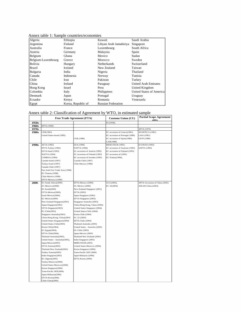
Annex table 1: Sample countries/economies

Annex table 2: Classification of Agreement by WTO, in estimated sample

Algeria Ethiopia Kuwait Saudi ArabiaArgentina Finland Libyan Arab Jamahiriya SingaporeAustralia France Luxembourg South AfricaAustria Germany Malaysia SpainBelgium Ghana Mexico SudanBelgium-Luxembourg Greece Morocco SwedenBolivia Hungary Netherkands SwitzerlandBrazil Iceland New Zealand TaiwanBulgaria India Nigeria ThailandCanada Indonesia Norway TunisiaChile Iran Pakistan TurkeyChina Ireland Paraguay United Arab EmiratesHong Kong Israel Peru United KingdomColombia Italy Philippines United States of AmericaDenmark Japan Portugal UruguayEcuador Kenya Romania VenezuelaEgypt Korea, Republic of Russian Federation

Customs Union (CU) Partial Scope Agreement (PS)

1950s EC(1958),

1960s EFTA (1960)

1970s APTA (1976)

1980s CER(1983) EC accession of Greece(1981) SPARTECA (1981)United States-Israel (1985) EC accession of Portugal (1986) LAIA (1981)

CER (1989) EC accession of Spain(1986) GSTP (1989)CAN(1988)

1990s AFTA (1992) EEA (1994) MERCOSUR (1991) ECOWAS (1993)EFTA-Turkey (1992) NAFTA (1994) EC accession of Austrian (1995) SAPTA (1995)EFTA-Israel (1993) EC accession of Austria (1995) EC accession of Finland (1995)NAFTA (1994) EC accession of Finland (1995) EC accession of (1995)COMESA (1994) EC accession of Sweden (1995) EC-Turkey(1996),Canada-Israel (1997) Canada-Chile (1997)Turkey-Israel (1997) Chile-Mexico (1999)Canada-Chile (1997)Pan-Arab Free Trade Area (1998)EC-Tunisia (1998)Chile-Mexico (1999)EFTA-Morocco (1999)

2000- EC-South Africa(2000) EFTA-Mexico (2000) GCC(2003), APTA-Accession of China (2002)EC-Morocco(2000) EC-Mexico (2000) EC 25(2004) ASEAN-China (2003)EC-Israel(2000) New Zealand-Singapore (2001)EFTA-Mexico(2000), EFTA (2002)Israel-Mexico(2000), Japan-Singapore (2002)EC-Mexico(2000) EFTA-Singapore (2003)New Zealand-Singapore(2001) Singapore-Australia (2003)Japan-Singapore(2002) China-Hong Kong, China (2004)EFTA-Singapore(2003) United States-Singapore (2004)EC-Chile(2003) United States-Chile (2004)Singapore-Australia(2003) Korea-Chile (2004)China-Hong Kong, China(2004) EC 25 (2004)United States-Singapore(2004) EFTA-Chile (2004)United States-Chile(2004) Thailand-Australia (2005)Korea-Chile(2004) United States - Australia (2005)EC-Egypt(2004), EC-Chile (2005)EFTA-Chile(2004), Japan-Mexico (2005)Thailand-Australia(2005), Thailand-New Zealand (2005)United States - Australia(2005), India-Singapore (2005)Japan-Mexico(2005) MERCOSUR (2005)EFTA-Tunisia(2005) United States-Morocco (2006)Thailand-New Zealand(2005) Korea-Singapore (2006)Turkey-Tunisia(2005) Trans-Pacific SEP (2006)India-Singapore(2005) Japan-Malaysia (2006)EC-Algeria(2005) EFTA-Korea (2006)Turkey-Morocco(2006)United States-Morocco(2006)Korea-Singapore(2006)Trans-Pacific SEP(2006)Japan-Malaysia(2006)EFTA-Korea(2006)Chile-China(2006)

Free Trade Agreement (FTA)

1

Annex table 3: Weighted average of tariff rate, MNF rate, all country

Data: TRAINS by UNCTAD Annex table 4: Simple average tariff rate during 1988-2006

Notes: Simple average tariff rate of sample countries, during 1988-2007, calculated by data from TRAINS by UNCTAD.

1990 1995 2000 2005 2006 Simple average on five periods

SITC01 Meat and meat preparations 12.13 19.22 16.74 13.47 11.78 14.7SITC04 Cereals and cereal preparations 9.96 7.99 12.33 11.27 21.19 12.5SITC05 Vegetables and fruit 13.15 12.1 10.48 9.59 10.05 11.1SITC24 Cork and wood 2.13 1.33 1.27 1.17 1.17 1.4SITC26 Textile fibres and their waste 2.99 3.46 5.85 8.07 12.44 6.6SITC33 Petroleum,petroleum products 2.81 3.85 2.76 2.54 1.99 2.8SITC51 Organic chemicals 9.82 6.83 4.62 4.21 3.83 5.9SITC52 Inorganic chemicals 6.25 4.47 3.53 3.21 2.71 4.0SITC54 Medicinal and pharmaceutical products 6.94 2.02 1.51 1.26 1.02 2.6SITC63 Cork and wood, cork manufactures 7.62 6.78 4.76 4.78 4.71 5.7SITC65 Textile yarn, fabrics, made-up articles 16.56 11.38 13.03 9.25 8.74 11.8SITC67 Iron and steel 8.9 6.07 5.5 4.43 3.61 5.7SITC68 Non-ferrous metals 4.13 3.31 3.19 3.05 2.71 3.3SITC74 General industrial machinery 7.39 5.93 5.13 4.06 3.78 5.3SITC75 Office machines and equipment 4.17 2.5 1.01 0.32 0.29 1.7SITC76 Telecommunications equipment 7.79 6.3 4.09 2.72 2.44 4.7SITC77 Electric machinery 7.33 5.06 3.34 1.94 1.73 3.9SITC78 Road vehicles 7.17 8.7 7.64 8.64 8.47 8.1SITC84 Articles of apparel 16.26 13.08 13.11 11 11.01 12.9SITC87 Professional and scientific instruments 6.59 5.17 3.01 3.14 3.02 4.2

Averag S.D. Averag S.D. Averag S.D. Averag S.D.SITC01 Meat and meat preparations 13.40 (17.51) 12.32 (16.46) 20.51 (24.56) 22.03 (24.77) SITC04 Cereals and cereal preparations 11.49 (13.09) 11.26 (15.10) 20.50 (18.59) 20.25 (16.98) SITC05 Vegetables and fruit 12.73 (12.24) 12.13 (12.87) 20.48 (19.57) 20.57 (18.83) SITC24 Cork and wood 3.06 (5.01) 2.86 (4.79) 8.43 (9.02) 9.07 (9.67) SITC26 Textile fibers and their waste 3.78 (5.05) 3.21 (4.80) 11.47 (11.38) 12.56 (12.50) SITC33 Petroleum, petroleum products 4.14 (3.88) 4.00 (3.73) 9.46 (9.76) 10.43 (9.87) SITC51 Organic chemicals 4.35 (3.90) 4.39 (4.40) 9.39 (8.75) 9.36 (8.86) SITC52 Inorganic chemicals 3.52 (4.04) 3.47 (4.00) 9.49 (9.46) 9.45 (9.16) SITC54 Medicinal and Pharmaceutical products 2.57 (3.66) 2.59 (3.78) 9.17 (8.82) 9.16 (8.82) SITC63 Cork and wood manufactures 6.86 (5.80) 6.88 (5.93) 17.69 (12.06) 17.98 (12.83) SITC65 Textile yarn, fabrics, made-up articles 10.40 (5.58) 10.47 (5.77) 20.84 (14.11) 20.95 (14.39) SITC67 Iron and steel 4.93 (4.37) 4.90 (4.40) 13.33 (9.98) 13.38 (10.02) SITC68 Non-ferrous metals 4.63 (3.89) 4.40 (3.98) 11.00 (9.29) 11.63 (9.22) SITC74 General industrial machinery 4.82 (4.33) 4.64 (4.32) 12.19 (9.55) 12.06 (9.09)

SITC75 Office machines and automatic data processing equipment

2.54 (4.04) 2.35 (3.92) 8.83 (10.35) 9.39 (11.95)

SITC76 Telecommunications, sound recording & reproducing equipment

5.69 (5.43) 5.32 (5.29) 15.54 (12.05) 15.62 (12.24)

SITC77 Electric machinery 5.03 (4.54) 4.75 (4.52) 14.47 (10.51) 14.68 (10.30) SITC78 Road vehicles 6.97 (6.63) 6.80 (6.45) 21.36 (19.94) 20.95 (17.54) SITC84 Articles of apparels 16.84 (7.73) 16.77 (7.83) 24.55 (16.46) 25.48 (17.73) SITC87 Professional and scientific instruments 3.89 (3.97) 3.73 (4.01) 9.47 (7.83) 9.49 (7.74)

G77

Tariff rate btwn G77 countries

Tariff rate against all countries

Commodity Developed countries Tariff rate against all countries

Tariff rate btwn developed countries