Trade Costs, Pricing to Market, and InternationalRelative Prices∗†

Andrew Atkeson‡and Ariel Burstein§

February, 24 2005

Abstract

We extend some of the recently developed models of international trade to studytheir implications for the main features of the fluctuations in the relative producerand consumer prices of tradeable and traded goods observed in the data. We findthat when our model is parameterized to match some of the main features of thedata on trade volumes both at the aggregate and firm level and to have reasonableimplications for both the concentration of production among producers in a marketand the distribution of markups of price over marginal cost, it reproduces many of themain features of the data on the fluctuations in the relative producer and consumerprices of tradeable and traded goods. We then use this model to assess the extent towhich international trade costs and imperfect competition with pricing to market playessential roles in accounting for these price data. We find that international trade costsplay an essential role in our model in accounting for the behavior of both producer andconsumer prices for tradeable and traded goods. We find that imperfect competitionwith pricing to market plays an essential role in accounting for the behavior of producerprices for tradeable and traded goods, but it plays only a minor role in accounting forthe behavior of consumer prices of tradeable goods.

∗Very preliminary and incomplete. Please check the authors’ websites for more up to date versions of thispaper.

†We thank V.V. Chari and Marc Melitz for very useful comments and Ricardo Pasquini and Sergio Xavierfor excellent research assistance.

‡UCLA, Federal Reserve Bank of Minneapolis, and NBER.§UCLA.

1. Introduction

The hypothesis of purchasing power parity (PPP) – at least in its loosest form as the

hypothesis that international trade in goods should limit the fluctuations in the relative price

of tradeable goods across countries – has been a central pillar of standard open-economy

macroeconomic models for many years. This hypothesis of purchasing power parity appears

to give a very good account of the fluctuations in the international relative prices of gold or

oil or several other traded commodities – the relative prices of gold or oil across countries,

stated in terms of a common currency, are essentially constant. It has been clear for several

decades, however, that the hypothesis of purchasing power parity gives a poor account of

the fluctuations in international relative prices at the aggregate level: real exchange rates,

measured in terms of consumer prices, producer prices, or relative costs of production across

countries are all extremely volatile. It has been argued in the literature that consideration of

international trade costs and imperfect competition leading to pricing to market1 are likely

to be key components of a successful model of these movements in international relative

prices (see, for example Obstfeld and Rogoff 2000 and Engel 2002).

In this paper, we extend some of the recently developed models of international trade to

study their implications for the main features of the fluctuations in the relative producer and

consumer prices of tradeable and traded goods observed in the data. In particular, our model

nests versions of both the older models of trade based on specialization and monopolistic

competition surveyed in Helpman and Krugman (1985) and the newly developed extensions

of Dornbush, Fisher, and Samuelson’s (1977) Ricardian model of international trade with a

continuum of goods by authors such as Eaton and Kortum (2001), Bernard, Eaton, Jensen

and Kortum (2003), Melitz (2003), Eaton, Kortum, Kramarz (2004), and Alvarez and Lucas

(2004).

Our model follows this earlier work in providing a simple and tractable account of the

patterns of international trade both at the aggregate level and at the level of the individual

producer. It also includes a simple yet rich model of imperfect competition in which firms do

not fully pass through changes in their marginal costs to their prices and in which exporting

firms may practice pricing to market. Our model features a large number of sectors each with

a finite number of firms producing differentiated products within the sector, with these firms1Pricing to market is defined as fluctuations in the relative price (measured in the same currency) that an

exporter charges for his output in two different markets. See, for example, Dornbush (1987) and Krugman(1987) for an early discussion of this pricing practice.

2

engaged in quantity competition a la Cournot2. We ask whether this model can reconcile

observed patterns of international trade with fluctuations in international relative prices3.

It is important to note that our approach in this paper is partial equilibrium in the sense

that we take as given movements in the relative cost of production across countries and ask

what changes in the consumer and producer prices of tradeable and traded goods should

result from these changes in costs. We do not address in this paper the general equilibrium

question of what shocks lead to these large and persistent changes in costs and prices across

countries.

We find that a version of our model parameterized to match some of the main features

of the data on trade volumes both at the aggregate and firm level and to have reasonable

implications for both the concentration of production among producers in a market and the

distribution of markups of price over marginal cost reproduces many of the main features

of the data on the fluctuations in the relative producer and consumer prices of tradeable

and traded goods. We then use the model to assess the extent to which international trade

costs and imperfect competition with pricing to market play essential roles in accounting for

these price data. We find that international trade costs play an essential role in our model in

accounting for the behavior of both producer and consumer prices for tradeable and traded

goods. We find that imperfect competition with pricing to market plays an essential role in

accounting for the behavior of producer prices for tradeable and traded goods, but it plays

only a minor role in accounting for the behavior of consumer prices of tradeable goods.

We focus on two features of the data on international relative prices in particular. The

first feature of the data is the observation that, for the major developed economies, the

international relative producer price of manufactured (tradeable) goods is substantially more

volatile than the corresponding terms of trade for manufactured goods. In our model, the

international relative producer price of tradeable goods moves in response to a change in

relative production costs across countries simply because each country specializes in the2Feenstra, Gagnon, and Knetter (1996) and Yang (1997) study related models of imperfect competiton

with variable markups. Bergin and Feenstra (2001) and Corsetti and Dedola (2003) also present frameworksfor analyzing monopolistic competition with non-constant elasticities of demand. Variable markups are alsoa characteristic of the literature on exchange rates and sticky prices (see for example Betts and Devereux2000 and Chari, Kehoe and McGrattan 2002). Our work is distinguished from that sticky-price literature inthat here prices are always set optimally and not fixed by assumption.

3Bergin and Glick (2004) and Ghironi and Melitz (2004) also study versions of new models of internationaltrade that can account for some features of fluctuations in international relative prices. Their main emphasisis on the role of the entry and exit of firms to the export markets. Here we focus on trade costs and variablemarkups leading to pricing to market by individual firms.

3

production of a distinct set of goods. What is more difficult to reproduce in the model

is the observation that this change in relative production costs across countries leads to a

substantially smaller movement in the terms of trade. Algebraically, this can be the case only

if there are systematic fluctuations in the ratio of export prices to home country producer

prices and the ratio of import prices to source country producer prices for tradeable goods.

In the context of our model, this feature of the data can be explained only if there are

costs of international trade and if exporting firms practice substantial pricing to market. To

see this, observe that if firms set both domestic and export prices at a constant (but perhaps

different) markup over marginal cost, then they do not practice pricing to market and shocks

to marginal cost leave the ratio of export prices to producer prices in each country unchanged.

Hence relative producer prices and the terms of trade move one-for-one with each other. Next

observe that in our model, even if firms charge variable markups in that they do not raise

prices one-for-one with a change in marginal cost, in the absence of international trade costs,

firms face the same set of competitors when selling at home and abroad and thus choose

identical markups and prices in both markets. Thus, without international trade costs, we

have no pricing to market. We see the finding that our model of imperfect competition and

international trade can, with reasonable parameter values, reproduce this observation about

the fluctuations in the international relative producer price of tradeable and traded goods,

as one of the major results of the paper.

The second feature of the data that we study is the finding that for many developed

economies there appears to be little or no difference in the magnitude of the fluctuations in

the international relative consumer price of the basket of goods that are considered tradeable

and the magnitude of the fluctuations in consumer price based real exchange rates4. This

finding has been presented as an important challenge in open economy macroeconomics since

it suggests that international arbitrage through international trade plays only a very limited

role in mitigating the fluctuations in international relative consumer prices at the macro-

economic level. We find, in the context of our model, that there is a simple explanation for

this finding regarding the behavior of consumer prices in the data – goods that are actually

traded form only a small share of the cost of the CPI bundle that is considered tradeable5.4This observation that the fluctuations in the international relative consumer price of tradeable goods

are nearly as large as fluctuations in CPI-based real exchange rates themselves holds both at short and longhorizons. See, for example, Engel (1999), Obstfeld and Rogoff (2000), Chari, Kehoe, McGrattan (2002), andBetts and Kehoe (2004).

5Standard models in open economy macro like those studied by Backus, Kydland, and Kehoe (1995)

4

This is true not only because imports are only a relatively small share of domestic output

(measured at producer prices) of tradeables sectors, but also because consumer prices for

tradeables include a substantial margin over producer prices accounted for by non-tradeable

distribution services (see Burstein, Neves, and Rebelo 2003 and Burstein, Eichenbaum, and

Rebelo 2004 for a related argument to explain low inflation after large devaluations).

We find in our model that consideration of pricing to market under imperfect compe-

tition contributes very little to the movements in the relative consumer price of tradeable

goods. This is because this pricing has two nearly offsetting effects on the consumer price

of tradeables. Pricing to market leads to movements in the ratio of export and producer

prices that amplify the movement in the relative consumer price of tradeables in response to

a change in international relative costs. It also leads, however, to movements in the markups

that firms charge for domestic sales that dampen the movement in the relative consumer

price of tradeables in response to a change in international relative costs.

After considering these macro implications of our model for international relative prices,

we then study the implications of our model for producer prices and the terms of trade at

the sectoral level. We find in sectoral data for the U.S. manufacturing sector that there is

tremendous heterogeneity in the movements in the ratios of export and import to producer

prices that occur even when there is a large change in the producer price based real exchange

rate for the U.S. Moreover, this heterogeneity does not appear to be strongly related either

to the share of sectoral output that is traded or to the Herfindahl index for the sector as a

measure of its concentration. We find similar results for the sectors in our model. We find

that there is considerable heterogeneity across sectors in the responses of export, import, and

producer prices to our assumed change in relative costs across countries. We also find that

these heterogeneous responses are not tightly linked to the share of sectoral output that is

traded or to the Herfindahl index for the sector. Pricing in our model, it turns out, depends

in subtle ways on the exact configuration of costs across firms in a sector, and this is true

despite the relative simplicity of our formulation.

The structure of our paper is as follows. We first review the observations on international

relative prices that are the focus of this paper. We then present our model. Here we abstract

from consideration of non-tradeable distribution costs in the consumer prices of tradeable

if extended to include a non-tradeable sector and calibrated to have a small share of foreign goods inthe tradeable aggregate would also be consistent with the observation that the relative consumer price oftradeables is almost as volatile as the real exchange rate.

5

goods to keep the model simple. We present a parameterization of the model that roughly

matches micro and macro observations on the extent of trade in US manufacturing as well

as data on industry concentration and firm markups and then consider the implications of

this model for the relative producer and consumer prices of tradeable and traded goods

in response to a change in the relative costs of production across countries. To illustrate

the role of pricing to market and international trade costs in the model, we compare our

results to two alternative parameterizations of the model – one in which firms choose prices

that are a constant markup of prices over marginal cost and another in which there are no

international trade costs. We next examine the pricing implications of the model at the

sectoral level and compare them to sectoral level price data from the U.S.. We then conduct

a sensitivity analysis of how our quantitative results for both micro and price data depend

on the parameters of the model. Here we also explore the pricing implications of our model

at the firm level. Finally, we extend the model to include non-tradeable distribution costs

in the pricing at the consumer level of tradeable goods.

2. Data on International Relative Prices

Fact 1: The manufacturing terms of trade are significantly less volatile than the

international relative price of manufactured goods

The terms of trade (TOT ) for a given country is the ratio of the price index for imported

goods (IPI) to the price index for exported goods (EPI). One can think of these import and

export price indices as trade-weighted indices of the prices of goods actually traded with that

country’s trading partners. In Table 1, we compare the volatility of the terms of trade for

manufactured goods for a number of developed countries to the volatility of the international

relative price of manufactured goods for these countries. For each country, we measure the

international relative price of manufactured goods as the ratio of the producer price index for

manufactured goods for that country (PM) to a trade-weighted6 average of the manufactured

goods producer price indices for that country’s trading partners, where these price indices

are measured in the currency of the home country (eP ∗M). This international relative price of

manufactured goods can be thought of as a PPI-based real exchange rate for manufactured

goods. Manufactured import and export prices as well as manufacturing producer price

indices are obtained from the OECD. We also include additional results in the table for the6We use trade weights obtained from the OECD.

6

United States using manufactured import and export price indices computed by the Bureau

of Labor Statistics (BLS)7. We use import and export price indices for manufactured goods

to be consistent with our model and to avoid including oil prices which have a large impact

on the volatility of the overall terms of trade for many countries (see Backus and Crucini

2000).

Figure 1 displays quarterly time series using BLS data, between 1985 and 2004, for the

U.S. terms of trade for manufactured goods and the U.S. trade weighted manufacturing PPI-

based real exchange rate. Table 1 shows the relative volatility of the manufacturing terms

of trade and trade weighted manufacturing PPI-based real exchange rates for a variety of

countries. Volatilities in the table are measured both in terms of the standard deviation of

four quarter changes in prices and in terms of the standard deviation of deviations of prices

from HP-trends. It can be seen both in the table and the figure that movements in the

terms of trade are significantly smaller than changes in the international relative price of

manufactured goods.

Algebraically, this can be the case only if there are systematic fluctuations in the ratio

of export prices to home country producer prices and the ratio of import prices to source

country producer prices for tradeable goods. This implication follows from the decompositionµPMeP ∗M

¶=

µPMEPI

¶µIPI

eP ∗M

¶µEPI

IPI

¶. (2.1)

In this decomposition, PM/eP ∗M is the international relative producer price of tradeable

goods, PM/EPI is the ratio of producer and export prices for tradeable goods, IPI/eP ∗Mis the (trade weighted) ratio of import and foreign producer prices for tradeable goods, and

EPI/IPI is the terms of trade8.

As is to be expected given the findings above, in our data, there are large fluctuations in

the price ratios PM/EPI and IPI/eP ∗M .We report on the magnitude of these fluctuations in7The Bureau of Labor Statistics (BLS) constructs import and export price indices for the United States

using sampling methods similar to those that it uses to compute producer price indices. In many othercountries, the prices of imports and exports are measured using unit values rather than price indices. Incontrast with the BLS data, the OECD data on import and export prices is in terms of unit values.

8This decomposition has been studied in the sticky price literature on the fluctuations in internationalrelative prices. Obstfeld and Rogoff (2000) have observed that if one assumes that nominal prices are stuckin the currency of the producing firm, then the ratio of nominal export prices to producer prices in eachcountry is fixed and hence the relative price of tradeable goods and the terms of trade move together one forone with any movement in the nominal exchange rate. In contrast, if nominal prices are stuck in the currencyof the country in which the good is sold, then a shift in the exchange rate leads to an equivalent shift in theratio of export prices to domestic prices in each country and the terms of trade moves one-for-one, but inthe opposite direction, as the relative price of tradeable goods. As noted by Campa and Goldberg (2004),the data lie between these two extremes.

7

Table 1 as well. Figure 2 displays large fluctuations of IPI/eP ∗M in the U.S. for manufacturing

imports from Japan, the European Union, and Canada. Manufacturing price indices by

locality of origin were obtained from the BLS.

We think of this finding that there are systematic fluctuations in the ratio of export to

domestic prices across countries as the macroeconomic analog of the finding in the literature

that there is pricing to market in firm level or highly disaggregated price data. In terms

of that literature Marston (1990) studies the response of domestic and export prices to

changes in Japan’s real exchange rate, for 17 4-digit Japanese industries. On average, his

estimates imply that the relative price of exports to domestic sales falls by roughly 50% of

any appreciation of the real exchange rate. Knetter (1990 and 1993) studies how prices of

exports from U.S., UK, Japan, and Germany, response to changes in destination specific real

exchange rates. He finds, for example, that the relative price that Japanese auto exporters

charge for their exports in Germany relative to the U.S., change by 70% of any fluctuation

in the Germany-U.S. real exchange rate. Goldberg and Knetter (1997) survey recent micro

studies that suggest that pricing to market is very prevalent in the data.

Fact 2: Fluctuations in CPI-real exchange rate for tradeable goods across

countries are nearly as large as fluctuations in overall CPI-real exchange rates

Our first fact concerns producer prices – the prices that firms charge for goods that

are internationally traded and goods that are sold domestically. Our second fact concerns

consumer prices. Define the CPI-real exchange rate (RER) as the ratio of the consumer

price indices (CPI) in two countries, measured in a common currency, and define the CPI-

real exchange rate for tradeable goods as the ratio of the component of the CPI covering

tradeable goods in those two countries, again measured in a common currency. Engel (1999)

and Betts and Kehoe (2002) propose an approach to decompose movements in the real

exchange rate into two components: movements in the relative price of tradeable goods

across countries, and movements in the price of non-tradeables relative to tradeables across

countries:

RER =P1eP2

=

µP T1eP T2

¶µP1/P

T1

P2/P T2

¶(2.2)

=¡RERT

¢ ¡RERN

¢Here, P Ti denotes that component of the CPI in country i that is categorized as tradeable

and e the nominal exchange rate. The term Pi/PTi is proportional to the the price of non-

tradeables relative to tradeables across countries. Non-tradeable goods account on average

8

for roughly 50 percent of the CPI basket (60% in the U.S.), and include categories like

education, health, and housing. Tradeables include non-durable goods (food and beverages,

apparel, etc.) and durables (private transportation, household furnishings, etc.). Work by

Engel (1999), Obstfeld and Rogoff (2000), Betts and Kehoe (2002), and Chari, Kehoe, and

McGrattan (2002) find that RERT is almost as volatile as RER for a set of industrialized

countries. Engel (1999) examines U.S. bilateral real exchange rates with a set of OECD

countries, and finds that at short and medium horizons, RERT accounts for almost all

fluctuations in the mean squared error of changes in RER. Chari, Kehoe and McGrattan

(2002) let country 1 be the United States, and country 2 be an aggregate of four European

countries. Using a sample period from 1973 to 1998, they find that the standard deviation

of detrended RERT is 94% as large as the standard deviation of RER.

It is important to note that a model such as the one that we study has very different

implications for the fluctuations in the international relative price of tradeable goods as mea-

sured by producer prices and the international relative price of tradeable goods as measured

by consumer prices. In our model, each country specializes in the production of a different

set of commodities with that set determined by comparative advantage. If the relative cost

of production across countries fluctuates, then there are fluctuations in the international rel-

ative producer prices of tradeable goods as firms change their prices in response to changes

in cost. These fluctuations in the producer prices for tradeable goods occur even if the law

of one price holds for each tradeable good simply because the set of goods being produced is

different in each country. In contrast, in the absence of international trade costs, if the law

of one price holds, there are no fluctuations in the international relative price of tradeable

goods as measured by consumer prices because, in the model, the set of tradeable goods

consumed in each country is identical.

3. The Model

We develop a partial equilibrium model in which two symmetric countries (indexed by

i = 1, 2) produce and trade a continuum of goods subject to frictions in international goods

markets. We first illustrate our results in a simple version of the model to keep the intuition

for our results clear. In particular, we leave out until Section 8 consideration of the role

of non-traded distribution costs in affecting pricing of tradeable goods. We consider aggre-

gate shocks to the marginal cost of production as the driving force behind fluctuations in

9

international relative prices.

3.1. Aggregation of goods into sectors

Our model is designed to allow us to derive implications for international relative prices

both at an aggregated and disaggregated level. At the lowest level of disaggregation in our

model, we consider individual firms producing what we term goods. These goods are the

only commodities in our model that should be interpreted as physical objects that can be

traded across international borders.

We aggregate goods into categories that we term sectors. We interpret sectors in our

model as corresponding to the lowest level of disaggregation of commodities used in economic

censuses and price index construction. We assume that each firm in our model produces a

distinct good in a specific sector. One important assumption that we make is that there are

only a relatively small number of firms in each individual sector.

We then further aggregate sectors into two consumption composites: one that we call

tradeable consumption and the other non-tradeable consumption. We interpret the prices

in our model of these two consumption composites as corresponding to the tradeable and

non-tradeable components of the consumer price index in the data studied by Engel (1999)

and others. Finally, at the highest level of aggregation, these two consumption composites

are combined into aggregate consumption, the price of which in the model corresponds to the

consumer price index in the data.

We present this aggregation of goods starting at the highest level of aggregation as follows.

Aggregate consumption ci is an aggregate of two consumption composites: tradeable con-

sumption cTi , and non-tradeable consumption cNi given by

ci =¡cTi¢γ ¡

cNi¢1−γ

.

The price of aggregate consumption at date t, which we interpret as the consumer price

index, is denoted Pit and is given by Pi = κ¡P Ti¢γ ¡

PNi¢1−γ

, where κ = γ−γ (1− γ)−(1−γ)

and P Ti is the component of the consumer price index covering tradeable goods and PNi is

the component of the consumer price index covering non-tradeable goods.

The tradeable and non-tradeable consumption composites cTi and cNi are produced by a

competitive firm using the products of a continuum of sectors yTij and yNij for j ∈ [0, 1] as

10

inputs subject to a standard CES production function

cTi =

·Z 1

0

¡yTij¢1−1/η

dj

¸η/(η−1)and cNi =

·Z 1

0

¡yNij¢1−1/η

dj

¸η/(η−1). (3.1)

As is standard, the tradeable and non-tradeable price indices P Ti and PNi are given by

P Ti =

·Z 1

0

¡P Tij¢1−η

dj

¸1/(1−η)and PNi =

·Z 1

0

¡PNij¢1−η

dj

¸1/(1−η)(3.2)

and the demand functions for the output of individual sectors are given by

P TijP Ti

=

ÃyTijcTi

!−1/ηand

PNijPNi

=

ÃyNijcNi

!−1/η. (3.3)

We finally turn to the lowest level of aggregation in the model, the aggregation of goods

into sectors. In each country i and sector j, there are K domestic firms selling distinct goods

in the sector. For the non-tradeable sectors, the K domestically produced goods are the only

goods in these sectors. For the tradeable sectors, there are K domestic firms selling distinct

goods and an additional K foreign firms that may, in equilibrium, sell goods in that sector.

We use the convention that firms k = 1, 2, . . . ,K are domestic and k = K+1, K+2, . . . , 2K

are foreign. Output in each sector is given by

yTij =

"2KXk=1

¡qTijk¢ ρ−1

ρ

#ρ/(ρ−1)and yNij =

"KXk=1

¡qNijk¢ρ−1

ρ

#ρ/(ρ−1)(3.4)

where qTijk and qNijk are the sales in country i of firm k in tradeable (T ) and non-tradeable

(N) sectors j respectively. Again, as is standard, the sectoral price indices P Tij and PNij are

given by

P Ti =

"2KXk=1

¡P Tijk

¢1−ρ#1/(1−ρ)and PNi =

"KXk=1

¡PNijk

¢1−ρ#1/(1−ρ)(3.5)

and the demand functions for goods within a sector are given by

P TijkP Tij

=

ÃqTijkyTij

!−1/ρand

PNijkPNij

=

ÃqNijkyNij

!−1/ρ. (3.6)

3.2. Production and International Trade Costs

We assume that each firm has a constant returns to scale production function that has

labor as the only input. These production functions are given by zl, where z differs across

11

firms. Specifically, we assume that each firm draws its productivity z from a log-normal

distribution, with log z ∼ N(0, θ). We assume that the wage rate in country i is given byWi. Thus, the marginal costs of production for a firm with productivity z based in country

i is Wi/z.9

In addition to the production costs, we assume that there are two costs of international

trade. We assume that there is a fixed cost F for any firm that wishes to export any of its

output to the other country. We also assume that there is an iceberg type marginal cost of

exporting indexed by D ≥ 1. With this iceberg trade cost, the marginal cost for a firm withproductivity z in country 1 to sell its output in country 2 is DW1/z. Note that with D = 1,

the marginal cost of sales is the same across countries. We assume that for the goods in the

non-tradeable sectors j,N, D =∞ so there is no international trade in these goods.

In the model, we assume that there is an exogenously given number K of domestic firms

in each sector each with idiosyncratic productivity draws z. Hence, for the non-tradeable

sectors, the total number of firms in each sector is fixed at K. The total number of firms,

both domestic and foreign, that sell positive amounts of their goods in each country in each

tradeable sector is determined endogenously in equilibrium – firms will choose to export if

it is profitable for them to do so.

3.3. Market Structure

We assume that the individual goods producing firms are engaged in imperfect competition.

In most of the results that follow, we take as a baseline case a model of imperfect competition

based on the following assumptions.

A1) Goods are imperfect substitutes: ρ <∞.A2) Goods within a sector are more substitutable than goods across sectors: 1 < η < ρ.

A3) Firms play a static game of quantity competition. Specifically, each firm k chooses its

quantity qTijk or qNijk taking as given the quantities chosen by the other firms in the economy,

as well as the domestic wage rate W, and the aggregated prices P Ti and PNi and quantities

cTi and cNi . Note that under this assumption, each firm does recognize that sectoral prices

P Tij and PNij and quantities y

Tij and y

Nij vary when that firm changes its quantity qTijk or q

Nijk.

We solve the model under these assumptions as follows. We start with the non-tradeable

sectors. For each non-traded sector j,N in country i, there are K domestic firms. We say9Given the partial equilibrium nature of our exercise, the labor input can be more broadly interpreted as

a composite of labor and capital services at a unit cost W .

12

that a vector of quantities qNijk and prices PNijk are equilibrium prices and quantities in that

sector if, for each firm l = 1, . . .K, with productivity zNijl, the quantity qNijl and price P

Nijl

solve the profit maximization problem

maxP,q

Pq − qWi/zNijl

subject to the demand function derived from (3.3) and (3.6)

µP

PNi

¶=

µq

yNij

¶−1/ρÃyNijcNi

!−1/ηwith yNi given by (3.4), with qNijl = q, and the other quantities qNijk taken as given, and

aggregate price PNi and quantity cNi fixed.

The vector of equilibrium prices for the sector can be found by solving the first order

conditions of this profit maximization problem given the wage rateWi and firm productivities

zNijk. These first order conditions give equations

PNijk =

"ηρ

η(ρ− 1)− sNijk (ρ− η)

#Wi

zNijk, (3.7)

where sNijk = PNijkq

nijk/

PKl=1 P

Nijlq

nijl is the market share of firm k in its sector10.

We use an iterative procedure to solve for the equilibrium prices and quantities for the

tradeable sectors. Such a procedure is required to determine how many foreign firms pay the

fixed trade cost to supply the domestic market. We illustrate this procedure for tradeable

sector j, T in country 1. We first solve for the equilibrium prices and quantities under the

assumption that only the lowest cost producer in sector j, T in country 2 exports his good to

country 1. In this case, we solve for the K prices for the domestic firms using equation (3.7)

with i = 1 and the one price for the lowest cost producer in country 2 (this firm is numbered

K + 1) using the equation

P T1jK+1 =

"ηρ

η(ρ− 1)− sN1jK+1 (ρ− η)

#DW2

zT2jK+1.

10>From (3.5) and (3.6), these market shares can be written as a function of prices

sNijk =

³PNijk

´1−ρPKl=1

³PNijl

´1−ρ .Hence (3.7) defines K non-linear equations in the K equilibrium prices PNijk.

13

Note here that the iceberg trade cost D scales up the marginal cost for this exporter. We

then check whether, at these prices and quantities, this lowest cost exporter in country 2

earns enough profits to cover the fixed cost11 F . If this lowest cost exporter does not earn

enough to cover the fixed cost, then, in equilibrium, there are no firms in sector j that export

their good from country 2 to country 1. If this lowest cost exporter does earn enough to cover

the fixed cost, then we repeat the procedure above under the assumption that the two lowest

cost firms in sector j in country 2 export to country 1. If, at these new prices, the second

lowest cost firm in country 2 does not earn a profit large enough to cover the fixed cost F,

then, in equilibrium, only the lowest cost firm in sector j in country 2 exports to country 1.

If that second lowest cost producer in country 2 does earn a profit large enough to cover the

fixed cost F, we repeat the procedure with the three lowest cost firms in sector j in country

2.

We use the computer to simulate the equilibrium in a large number of tradeable and

non-tradeable sectors.

3.4. Market Share and Markups

Assumptions A1 and A2 generate two of the key features of this model of imperfect com-

petition. The assumption A1 that ρ <∞ implies that goods within a sector are imperfect

substitutes so that each firm in a sector charges a distinct price for its product despite the

fact that firms are engaged in quantity competition. With each firm charging a distinct price,

we can construct in the model distinct sectoral producer price indices (covering prices that

domestic producers charge for all sales), import price indices (covering prices that foreign

firms charge for domestic sales), and export price indices (covering prices that domestic firms

charge for foreign sales).

The assumption A2 that ρ > η implies that that each firm’s markup of its price over

marginal cost is an increasing function of that firm’s market share within its sector. This

implication of the model is clearly seen in the pricing formula (3.7). In one extreme, if the

firm has a market share s approaching zero, its markup approaches the standard markup

ρ/(ρ−1) for a firm that perceives only the sectoral elasticity of demand. In the other extreme,if the firm has a market share s approaching one, its markup approaches the standard markup11We compute the equilibrium entry decisions for exporters only once with wages equal across countries.

When we do so, we express the fixed cost as a percentage of the aggregate quantity F/cTi so that we calculatethe equilibrium entry decisions for each sector separately.

14

η/(η−1) for a firm that perceives only the elasticity of demand across sectors. Firms with asectoral market share between zero and one choose a markup that increases smoothly with

that market share.

It is this assumption A2 that breaks the link between prices and costs in our model

and gives us the possibility that firms will not pass through changes in cost one-for-one into

prices. Specifically, if a single firm or a group of firms in a sector experience an increase

in marginal cost relative to the other firms in the sector, this firm or group of firms will

loose market share and hence decrease their markup in equilibrium. As a result, the prices

charged by this firm or group of firms will rise by less than the increase in their costs12.

Hence, the observation of incomplete pass-through of changes in costs to prices arises quite

naturally in our model in the context of understanding the effects of shocks to relative costs

across countries affecting the prices chosen by firms in these countries competing in a single

national market.

This feature of our model that generates incomplete pass through is not, by itself, enough

to generate pricing to market. To get pricing to market, we must have that a change in costs

for one firm or a group of firms leads to a change in markups for those firms that is different

in each market in which these firms compete. For that, we will need that this change in

costs results, in equilibrium, in different changes in each firm’s market share in each market

in which it competes. As we will see below, the result that this model can generate pricing

to market follows from very subtle nonlinearities in the model’s equilibrium conditions.

It is worth noting that if we make the alternative assumption that ρ = η, then our model

reduces to the standard model of monopolistic competition with a constant markup of price

over marginal cost given by ρ/(ρ− 1).We will present results from this model with constantmarkups to illustrate the quantitative importance of endogenous variation in markups in our

model. This model with ρ = η and hence constant markups is similar to the model studied

by Ghironi and Melitz (2004). Eaton and Kortum (2002) and Alvarez and Lucas (2004)

study similar models in which it is assumed that firms set prices equal to marginal cost. Our

model has similar implications for the movements in international relative prices under the

assumption that ρ = η, so that markups are constant, as it does under the assumption that

firms set prices equal to marginal cost.

With the assumption A3 that firms engage in quantity competition, our model nests the12Note that if costs rise by the same amount for all firms in a sector, then prices also all rise by that

amount and market shares and markups remain constant.

15

standard Cournot model as ρ gets large. This is because, as ρ approaches infinity, the distinct

goods in a sector become perfect substitutes and there is a single price in each country for

output in that sector. This Cournot model is similar to that studied in Eaton, Kortum, and

Kramarz (2004).

In this paper, we study pricing under the assumption of quantity competition. It is

straightforward to solve our model under the alternative assumption that firms engage in

price competition in the sense that they choose their price and quantity to maximize profits

taking the vector of prices (rather than quantities) chosen by the other firms as given. Under

this alternative assumption of price competition, in equilibrium firms choose a markup of

price over marginal cost given by

ρ− s(ρ− η)

(ρ− 1)− s (ρ− η)(3.8)

where s is the firm’s market share within the sector. Note that with ρ > η, this markup is

also an increasing function of the firm’s market share s, is equal to ρ/(ρ−1) with s = 0, andη/(η−1) with s = 1. Thus, the implications of our model for markups under price competitionare qualitatively similar to those under quantity competition. Under the assumption of price

competition and the assumption that the fixed cost of exporting (F ) is zero, our model nests

the standard Bertrand model as ρ gets large. This Bertrand model is similar to that studied

in BEJK (2003).

Note that in our model, 1/D ≥ P T1jk/P T2jk ≤ D. This is because markups in the exportmarket are never larger than in the domestic market. Since equilibrium price differentials

are lower than the cost of trading goods internationally, no third party has an incentive

to ship goods to arbitrage these price differentials across countries. Therefore, the fact that

consumers don’t have incentives to arbitrage price differentials across countries is an outcome

of the model, and not a consequence of assuming international market segmentation.

4. A quantitative example

Here we argue that a plausibly parameterized version of our model can reproduce the main

facts regarding international relative prices cited above. Specifically, we show that, in re-

sponse to an exogenous shock to relative wages across countries, this model implies (i) a

movement in the terms of trade that is much smaller than the movement in the relative price

of tradeable goods across countries, and (ii) a movement in the relative price of tradeable

16

goods that is quite large relative to the overall movement in the real exchange rate. Again,

we do not model the shock that leads to this change in relative wage costs across countries.

One might think of it as arising from a productivity shock or from a change in the exchange

rate in a model with sticky nominal wages.

4.1. Choosing benchmark parameters

We argue that our model is plausibly parameterized because it reproduces a number of

important patterns of trade, not only at the macro level, but also at the level of individual

firms, as well as facts regarding the total sales and measured labor productivity of exporting

versus non-exporting firms, markups of price over marginal cost, and industry concentration

observed in firm-level data. Note that since the mapping between the model parameters

and its implications for the facts under study is complicated and non-linear, we cannot

follow the standard calibration procedure of choosing each parameter individually to match

a separate fact. Instead, we have chosen directly as a benchmark one parameterization that

reproduces a wide range of observations. We discuss the role of each parameter in the model

by considering how the model’s implications for our facts of interest change vary with each

parameter from its benchmark value.

In this benchmark quantitative example, we set the parameters to the following values:

γ = 0.4, η = 1.01, ρ = 10, θ = 0.37, D = 1.44, F/cTi = 0.0003, and K = 20. The model’s

implications in a symmetric equilibrium (W1 = W2) and the corresponding statistics from

U.S. data are presented in Table 2.

In terms of the model’s macro implications, we consider the overall expenditure share on

tradeable consumption (given by P Ti cTi /Pici), and the ratio of total exports plus imports to

tradeable consumption. We compare these implications of the model to U.S. data on the

portion of tradeable consumption in total consumer expenditure and the average of exports

and imports relative to gross output in goods producing sectors13 – see Tables 3 and 6.

Note that the overall expenditure share on tradeable consumption in the model is pinned13The source of the data on the volume of trade as a fraction of gross output is Table 15 from June

2004’s Survey of Current Business: “Improved Annual Industry Accounts for 1998-2003”. We define thegood producing sectors aggregate as the sum of Agriculture, forestry, fishing, and hunting; Manufacturing;and Mining. Table 3 reports the value of 0.5 (exports + imports) / gross output for this aggregate sectorbetween 1998 and 2002. Our choice of 16.5% (which is lower than the average in this period) is consistentwith the fact that the share of trade in this sector has been steadily growing over time. In the model we areabstracting from trade in services, where 0.5 (exports + imports) / gross output = 1.3% on average in thisperiod.

17

down at 40% by the parameter γ. The overall volume of trade in our model is determined

by the tension between the gains from trade due to increased variety and the international

trade costs14. Since our model has two symmetric countries, in the absence of trade costs

D and F, half of tradeable output in each country would be exported. With more than two

symmetric countries, the share of tradeable output that is exported would be even larger.

Our macro observation on the overall volume of trade can be broken down, at the firm

level, into two components: the first being the fraction of firms that export any output at

all, and the second being the fraction of total output that exporting firms actually export.

In Table 2, we compare these implications of the model to U.S. data cited in Bernard and

Jensen (2004) regarding the fraction of U.S. manufacturing plants that export any output

at all and data from BEJK (2003) on the median fraction of total plant output that these

exporting plants export15. In our model, if F = 0, with ρ <∞, all firms producing tradeableoutput export some of their output. Thus, a positive fixed cost of exporting is required

to match the observation that only a minority of plants export. Holding fixed the other

parameters and the identity of those firms that do export, variations in the marginal trade

cost D change the fraction of firm output that an exporting firm exports.

In our model with trade costs, it is the firms that draw the lowest marginal costs of

production that choose to pay the costs to export. In equilibrium, these firms also tend

to charge lower prices in their home market, and thus to sell more output and to have a

higher market share in their home sector, than the firms that do not export. Since these

exporting firms tend to have a higher market share in their home sector, from (3.7), we see

that in the model, exporters tend to choose a higher markup of price over marginal cost.

As BEJK (2003) discuss in detail, this implication that exporters choose a higher markup

of price over marginal cost implies that exporters have higher labor productivity measured

as sales divided by employment than non-exporters16. We present the model’s implications

for the median sales and measured labor productivity of tradeable goods firms that export

versus the median sales and measured labor productivity of tradeable firms that do not14In our model, with ρ <∞, the gains from trade are due entirely to increased variety since, by assumption,

firms in each country produce a distinct set of goods. In the limit as ρ→∞, the model becomes Ricardianas the distinction between goods within a sector disappears.15As reported in Table 1 in Bernard and Jensen (2004), the fraction of exporters in total plants was 21%

in 1987 and 30% in 1992. We choose an intermediate value of 25%.16Here we are assuming that the fixed costs to export are not counted in the calculation of labor productiv-

ity. If one were to include these costs in the calculation of labor productivity, then the model’s implicationsfor the labor productivity of exporting versus non-exporting plants would be ambiguous.

18

export. We compare these implications of the model to U.S. data cited in BEJK (2003)

regarding the median sales and measured labor productivity of U.S. manufacturing plants

that export versus the median sales and measured labor productivity of U.S. manufacturing

plants that do not export. Eaton, Kortum, and Kramarz (2004) examine census data on

the export behavior of French firms. They observe that these French data do not censor out

small firms in the same way that the U.S. data from the census of manufactures does. They

find that median sales for exporters in these French data are 28 times the median sales for

non-exporters. This is much larger than the analogous figure of 4.8 from the U.S. data cited

in BEJK.

In our model, the parameter θ governs the dispersion of productivities across firms in a

sector while the parameters η and ρ govern the extent to which this dispersion in produc-

tivities results in a dispersion of market shares and markups across firms. Here we examine

the implications of these parameter choices not only for the size and productivity advantage

of exporters versus non-exporters but also for the dispersion of market shares and markups

across firms in a sector more generally. To summarize the dispersion of market shares across

firms in a sector, we report the median Herfindahl index17 across sectors in our model in

Table 2. In the first panel of Figure 3 we show a histogram of Herfindahl indices across

sectors. While we do not have comprehensive data to which to compare these implications

of our model for market concentration across sectors18, it is useful to note for comparison

purposes, that the U.S. Department of Justice, in its merger guidelines19 regards markets

with a Herfindahl index below 1000 to be “unconcentrated”, markets with a Herfindahl index

between 1000 and 1800 as “moderately concentrated”, and markets with a Herfindahl index

above 1800 to be “highly concentrated”. We regard these merger guidelines as a rough guide

to the level of concentration of markets at an economically meaningful level of aggregation

in the U.S. economy.

In Table 2, we also report the sales-weighted mean markup of price over marginal cost

across firms in our model. The average markup in our model is in line with average markups17The Herfindahl index for a sector is the sum of the squared market shares of the firms in that sector.18The Census Bureau computes Herfindahl indices for manufacturing sectors down to six digit NAICS

industries using data from the Census of Manufactures. In 1997, there were 473 6-digit NAICS industrieswith 282 firms in the median industry and 700 firms on average in each industry. The median Herfindahlindex across the these industries was 571 and the average of the Herfindahl indices across these industries was737. We interpret sectors in our model as being at a lower level of aggregation than these 6-digit industriesand thus expect a higher level of concentration on average within our sectors.19See in particular the discussion at http://www.usdoj.gov/atr/public/guidelines/horiz_book/15.html

19

assumed in standard macro models (see for example Christiano, Eichenbaum, and Evans

(2003)). In the second panel of Figure 3 we show a histogram of firm markups of price over

marginal cost.

4.2. Two alternative parameter settings

We also study the implications of our model with two alternative sets of parameter values

to illustrate the key economic forces at play in our benchmark example. These alternative

parameter choices together with the model implications for these parameter choices are also

presented in Table 2.

In our first alternative set of parameters, we set ρ = η. From (3.7), we see that in this

case, all firms choose a constant markup of price over marginal cost of ρ/(ρ − 1). We referto this parameterization of our model as the constant markup version of our model. These

parameters are chosen so that, in the symmetric equilibrium, the constant markup version of

our model has the same implications for the share of tradeables in consumption, the share of

exports in manufacturing output and the fraction of exporting firms in the tradeable sector

as the benchmark model. The value of ρ = η is roughly equal to the value used by BEJK

(2003). We consider this constant-markup version of our model to illustrate the role that

variable markups play in shaping our model’s implications for international relative prices.

In the second alternative set of parameters, we set D = 1 and F = 0. In this case, there

are no costs of international trade. We refer to this parameterization of our model as the

frictionless trade version of our model. We consider this frictionless trade version of our

model to illustrate the role that trade frictions play in shaping our model’s implications for

international relative prices.

4.3. The response of prices to a change in costs

We now consider the change in equilibrium international relative prices implied by a one

percent increase in wages in country 1 relative to country 2. We assume that these relative

wages W1/W2 are measured in a common currency20. The specific shock that we consider in

one in which W1 increases by one percent and W2 remains fixed.

In Table 4 we report on our benchmark model’s implications for the relative price move-20In this draft, for computational simplicity, we compute equilibrium at the new wage rates under the

assumption that the same set of firms export as under the symmetric equilibrium. We show later that themodel results do not depend in any important way on this assumption.

20

ments that are the focus of our study: (i) the movement in the terms of trade as a percentage

of the movement relative producer price of tradeable goods across countries, and (ii) the

movement in the relative consumer price of tradeable goods as a percentage of the overall

movement in the real exchange rate measured using consumer prices21. We also include in

the table the implications of the constant markup and the frictionless trade versions of our

model for these same relative price movements.

4.3.1. The terms of trade and the relative producer price of tradeables

In row 3 of Table 4, we see that our benchmark model produces a movement in the terms of

trade that is only 54% as large as the movement in the relative producer price of tradeable

goods across countries. This implication follows from the fact that firms in country 1 reduce

their markups on exports to country 2 relative to their markups on domestic sales while

firms in country 2 increase their markups on exports to country 1 relative to their markups

on domestic sales. This variation in markups by location can be seen in the aggregate price

indices in rows 1 and 2 of Table 4 where we report that the export price index for country

1 falls relative to the tradeable producer price index for country 1 while the import price

index for country 1 rises relative to the tradeable producer price index for country 2. These

movements in traded goods prices relative to tradeable producer prices are large in magnitude

– both are roughly 23% as large as the movement in the relative producer price of tradeable

goods across countries.

In rows 4, 5, and 6 of Table 4, we report the movements in the producer price index, the

export price index, and the import price index for country 1 all as a percentage of the change

in wages W1. There we see that producer prices in country 1 rise by more than export prices

(this is what gives us the pricing to market) but that both changes in prices are smaller than

the corresponding change in domestic costs of production. Note in row 6 that the import

price index also rises. This is true despite the fact that there has been no change in costs in

country 2.21We measure the change in producer prices for tradeable goods in our model using an expenditure-share

weighted average of the change in prices charged by domestic firms both for domestic sales and exports. Herewe are following the practice of the BLS of including prices for all sales by domestic firms, including salesto foreigners, in the producer price index. Likewise, we measure the changes in export and import pricesusing expenditure-share weighted averages of the change in prices charged by domestic firms for their exportsthe change in prices for imported goods. We measure the change in consumer prices using an expenditure-weighted share of the change in prices for all goods domestically consumed. For the non-tradable sectors,all of these goods are domestically produced, while for the tradeable sectors, these include domesticallyproduced goods and imported goods.

21

Looking at the entries in Table 4 for the corresponding price movements for our constant-

markup and frictionless trade versions of the model, we see that we need both variable

markups and trade frictions to deliver these implications for the relative producer prices for

tradeable and traded goods. In both of these alternative versions of our model, the movement

in the terms of trade is identical to the movement in the relative producer price of tradeable

goods across countries and the ratio of export prices to tradeable producer prices is constant

in both countries.

The logic behind this finding that the terms of trade move one-for-one with the inter-

national relative producer price of tradeable goods differs across the constant markup and

frictionless trade versions of our model. In the constant markup version of our model, the

logic for this result is quite simple: for each firm, both domestic and export prices move

one-for-one with the movement in domestic wages. Hence all changes in marginal cost are

passed on fully to all prices. This feature of this constant-markup model can be seen clearly

in rows 4,5, and 6 of Table 4.

For the frictionless trade version of the model, the logic for this result is more subtle.

In this version of the model, markups are not constant – they vary with market share as

described in (3.7). Thus, it is not the case that changes in marginal cost are passed on fully

to prices. In fact, as is shown in rows 4 and 5 of the table there is incomplete pass-through as

the firms in the country with rising wages lose market share and hence reduce their markups

at home and abroad while we see in row 6 that the firms in the country with the constant

wages increase their prices for exports. With no trade frictions, however, the set of firms

competing in each sector is the same across countries, and this leads to the law-of-one price

for each good despite imperfect competition. More specifically, each firm in a sector has

the same marginal cost for sales in each country and hence each firm has identical market

shares, identical markups, and identical prices in each country. This implies that, for each

country, export prices remain constant relative to domestic producer prices and, thus, from

our decomposition (2.1), that the terms of trade are identical to the relative producer price

of tradeables across countries. Hence one can say that in the frictionless trade version of the

model, there is incomplete pass through of costs to prices, but no pricing to market. Note

as well that, in this model, international trade costs are not necessary for incomplete pass

through but they are necessary for pricing to market.

It is worth noting that in all three versions of our model, the relative producer price of

22

tradeable goods moves a great deal in comparison to the real exchange rate measured with

consumer prices. In our benchmark parameterization of the model, the relative producer

price of tradeable goods moves 87% as much as the CPI-based real exchange rate. In the

constant markup version of the model, it moves 115% as much as the CPI-based real exchange

rate, while in the frictionless trade version of the model, it moves by 90% as much as the

CPI-based real exchange rate. These results follow directly from the fact that in our model

each country specializes in the production of distinct sets of goods and hence there is no

sense in which the law of one price should hold for producer prices.

4.3.2. The real exchange rate and the relative consumer price of tradeable goods

We now turn to our model’s implications for movements in the relative price of tradeable

goods across countries when these prices are measured with consumer prices rather than

producer prices. In row 7 of Table 4, we see that our benchmark model produces a movement

in the relative consumer price of tradeable goods across countries that is 71% as large as

the movement in the overall consumer-price real exchange rate itself. Note that our model

produces this large movement in the relative consumer price of tradeable goods despite the

fact that it abstracts from non-tradeable distribution costs as a component of the consumer

price of tradeable goods. In Section 8, we extend the model to include these costs and obtain

the results listed in row 8 of Table 4. There we find that, with them included, the model

produces a movement in the relative consumer price of tradeable goods across countries that

is 87% as large as the movement in the overall consumer-price real exchange rate itself.

This finding in our benchmark model that the movement in the relative consumer price

of tradeable goods across countries is quite large stands in stark contrast to the implications

of the frictionless trade version of our model. As shown in row 7 of Table 4, in the frictionless

trade version of our model, the relative consumer price of tradeable goods does not move

at all. This is because in the frictionless trade version of the model, the law of one price

holds for each tradeable good and consumption baskets are identical across countries. Hence,

the consumer price index for tradeable goods is identical across countries. In this sense, the

introduction of costs of international trade has a dramatic impact on the pricing implications

of our model andmoves the model much closer to the data not only in terms of its implications

for traded quantities but also in terms of its implications for the relative consumer price of

tradeable goods across countries.

Note that this result that the consumer prices of tradeable goods are identical across

23

countries holds in the frictionless trade model even though, in that model, we have imperfect

competition with variable markups. Recall that with imperfect competition in our model,

there is incomplete pass through of foreign cost changes to import prices even in the fric-

tionless trade version of the model. Without these international trade costs, however, the

degree of pass through of costs to prices has no impact on our model’s implications for the

movements in the relative consumer price of tradeable goods.

Now consider the implications of our constant markup version of the model for movements

in the relative consumer price of tradeable goods. In row 7 of Table 4, we see that the

movement in the relative consumer price of tradeable goods is now 77% of the movement in

the overall consumer price real exchange rate. This movement in the constant markup version

of the model is even larger than it is in our benchmark model with variable markups. This is

because the pricing to market that arises in the benchmark model serves to dampen rather

than amplify the movement in the relative consumer price of tradeable goods. This finding

implies that while international trade costs are essential for generating movements in the

relative consumer price of tradeable goods, incomplete pass through and pricing to market

due to variable markups do not play an important role in generating this price movement.

This finding that pricing to market in our benchmark model serves to dampen rather

than amplify the movement in the relative consumer price of tradeable goods in comparison

to the constant markup version of the model can be understood as follows. Take as given

a change in the logarithm of relative wages across our two countries given by W1 − W2.

Let dPPIDTi denote the resulting change in the logarithm in the producer price index for

domestic sales of tradeable goods22 in country i, and dPPIDNi the corresponding change in

the producer price index for non-tradeable goods. Let dIPI and dEPI denote the change inthe logarithm of the import and export price indices for country 1. Then the change in the

consumer price index for tradeable goods in country 1 is given by

P T1 = (1− sM) dPPIDT1 + sMdIPI,

and that for country 2 by

P T2 = (1− sM) dPPIDT2 + sM dEPI,

22Recall that the standard producer price index includes the prices that domestic firms charge for exportsas well as the price that domestic firms charge for domestic sales. We use the term producer price index fordomestic sales here as a useful concept for explaining the intuition of our model.

24

where, with symmetry and balanced trade, sM is the share of tradeables expenditure on

imports in both countries. Hence, the change in the relative consumer price of tradeable

goods is given by

dRERT = (1− sM)³ dPPIDT1 − dPPIDT

2

´+ sM

³dIPI − dEPI´ .It is useful to rewrite this expression as

dRERT = (1− 2sM)³W1 − W2

´(4.1)

+(1− 2sM)³ dPPIDT

1 − W1 − dPPIDT2 + W2

´+sM

³dIPI − dPPIDT2 − dEPI + dPPIDT

1

´.

This equality decomposes the change in the relative consumer price of tradeable goods into

three components. The first component is simply the change in relative wages, which we

take to be exogenous. The second component depends on the degree to which the change

in relative wages, W1 − W2 is passed through to the prices paid for domestic sales in the

two countries as measured by dPPIDT1 − dPPIDT

2. The third component depends on the

degree of pricing to market as measured by the change in the relative price of exports and

domestic sales for each country given by dIPI − dPPIDT2 and dEPI − dPPIDT

1. Note that in

the frictionless trade version of our model, the import share sM = 1/2 so that the first two

components are zero and that in this model there is no pricing to market, so the third term

is zero as well.

For non-tradeable goods PNi = dPPIDNi, so the change in the real exchange rate is given

by dRER = γ dRERT + (1− γ)³ dPPIDN

1 − dPPIDN2

´,

where γ is the consumption expenditure share on tradeable goods.

The breakdown of the fluctuation in the relative consumer price of tradeable goods in (4.1)

is reported in rows 9, 10, and 11 of Table 4. Consider first the pricing in the constant markup

version of our model. In that model, all goods prices move one-for-one with movements

in marginal costs. Thus, the prices charged for all domestic sales move one-for-one with

domestic wages ( dPPIDTi = dPPIDN

i = Wi), and the terms of trade for country 1 also

moves by the change in relative wages³dEPI −dIPI´ = ³W1 − W2

´, so there is complete

pass-through of cost changes to domestic prices and there is no pricing to market. Thus, the

25

movement in the relative consumer price of tradeable goods is given by the first component

alone dRERT = (1− 2sM)³W1 − W2

´.

The ratio of the percentage movement in the relative consumer price of tradeables to the

real exchange rate is given by

dRERTdRER =(1− 2sM)(1− γ2sM)

= 77%.

The last equality follows from our parameter choices of γ = .4 and sM = .165.

Now consider pricing in our benchmark model with variable markups. For non-tradeable

goods, we still have that prices move one-for-one with marginal costs so that dPPIDNi = Wi

just as in the constant markup case. With variable markups, however, we have that the

magnitude of dRERT depends on the degree of pass through of costs to domestic prices andthe degree of pricing to market as measured in (4.1). We have incomplete pass-through of

costs to domestic prices in our benchmark model since domestic producers in the country

with rising relative costs lower their markups at home as they lose market share to imports

while domestic producers in the country with falling relative costs raise their markups at

home as they gain market share. Hence we have¯ dPPIDT1 − dPPIDT

2

¯<¯W1 − W2

¯,

so that this second component in (4.1) is negative in our benchmark model with W1−W2 > 0

as reported in row 10 of table 4. We also have pricing to market so that with W1− W2 > 0,

we have dIPI − dPPIDT2 > 0 and dEPI − dPPIDT

1 < 0.

Therefore, the third component in (4.1) is positive as reported in row 11 of table 4. Hence,

in our benchmark model, we have two offsetting effects on the relative consumer price of

tradeable goods due to variable markups – a negative effect due to incomplete pass through

of costs to prices by domestic producers facing competition from imports, and a positive

effect due to pricing to market.

It is clear from our results comparing the benchmark model and the constant markup

version of our model that the main reason for the movement in the international relative

consumer price of tradeable goods is that the trade costs lead to a relatively low value of the

import share sM .

26

5. Sectoral pricing

In this section we compare the implications of our benchmark model for sectoral producer,

export, and import prices and to some of the main features of U.S. data on these price by

sector. We have obtained from the Bureau of Labor Statistics a sample of sectoral export,

import, and producer price indices broken down into selected 3-6 digit sectors using the

NAICS definitions of sectors23. One of the most striking features of the data is that there is

tremendous heterogeneity across sectors in terms of changes in the relative price of imports

and domestic production and changes in the relative price of exports and domestic production

even in periods in which there are large changes in relative producer prices across countries.

In Figure 4, we present a histogram across sectors of these relative price changes (∆IPI/∆PPI

and∆EPI/∆PPI) for three time periods in which there was a large change in the U.S. trade

weighted real exchange rate measured using manufacture producer price indices. These time

periods are 1985Q3 − 1988Q4, 1995Q2 − 2001Q4, and 2001Q4 − 2004Q2, and the corre-sponding changes in the US PPI-based real exchange rate were −38%, 23%, and −15%. Wechose these time periods to isolate particularly large movements in the overall PPI based real

exchange rate. During these periods, the change in the overall manufacturing import price

index relative to the change in the trade weighted PPI real exchange rate was 62%, 76%,

and −39% (it was 17%, 53%, and −32% for the overall export price index). The horizontal

axis in Figure 4 is the change in the ratio of import to producer prices or export to producer

prices over the time period as a fraction of the change in the PPI real exchange rate. As

is clear from this histogram there is tremendous dispersion in these relative price changes

across sectors.

In the data, these changes in sectoral prices do not appear to be correlated either with

trade shares or with sectoral concentration. To document this fact, in Figures 5 and 6we show

scatter plots across sectors of ∆IPI/∆PPI versus sectoral import shares, ∆EPI/∆PPI

versus sectoral export shares, and these two price changes versus sectoral Herfindahl indices

for the three time periods listed above. Here, again, these price changes are normalized by

the change in the overall PPI based real exchange rate for each time period.

Our benchmark model also produces heterogeneous movements across sectors in import

and export price indices relative to producer price indices. In Figure 7 we plot a histogram23The BLS is in the process of producing a more complete set of sectoral price indices based on the new

NAICS definitions of sectors. The data that they sent to us are early results from that project.

27

across sectors in our benchmark model of ∆IPI/∆PPI and ∆EPI/∆PPI in response to

our assumed one percent change in costs across countries. Note that our assumption that

vector of costs across firms in a sector is randomly drawn is the only reason in our model that

price movements are not identical across sectors. Otherwise in our model, the parameters

governing elasticities of demand and the number of firms in each sector are constant across

sectors.

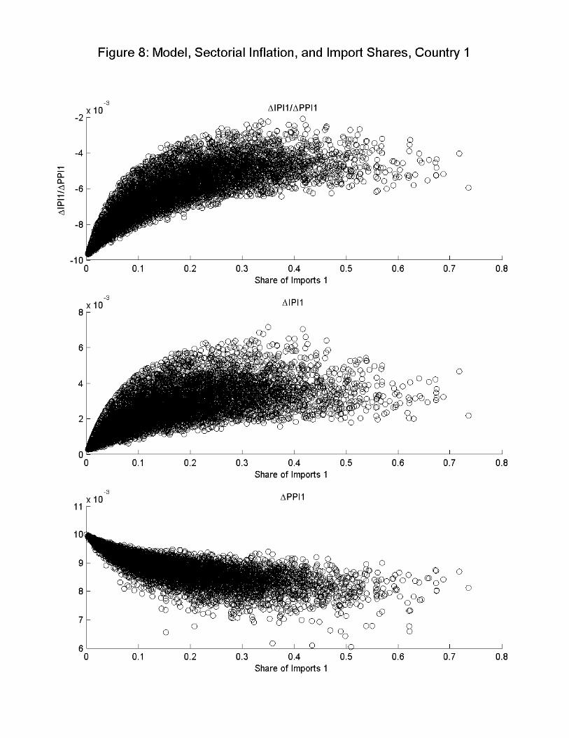
In Figure 8, we show scatter plots across sectors from our model of ∆IPI/∆PPI for

country 1 versus sectoral import shares, as well as ∆IPI and ∆PPI for country 1 individ-

ually versus sectoral import shares. Recall that in our experiment, wages in country 1 rise

by one percent relative to wages in country 2. We see in these figures that for sectors with

very small import shares, these two price indices move close to one-to-one with the changes

in cost: import prices do not change, producer prices rise by one percent, so that import

prices fall by one percent relative to producer prices. For sectors with larger import shares,

markups change so that prices do not move one-for-one with costs: import prices rise despite

the fact that costs in country 2 did not change, producer prices also rise, but now by less

than the full one percent change in costs, and the relative price of imports and domestic

sales falls, but by less (in absolute value) than for sectors with a very small import share. It

is worth noting in these figures, however, that there is considerable variation in the response

of prices in our model across sectors with the same import share.

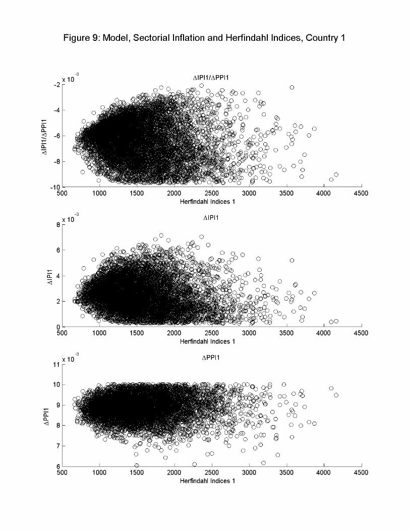
In Figure 9, we show the analogous scatter plots across sectors in our model with Herfind-

ahl indices rather than import shares on the horizontal axis. In these figures we see that

there is no close relationship in the model between sectoral concentration and price move-

ments. As should be clear from these model scatter plots, there details of the distribution

of costs across firms play an important role in determining sectoral price responses. These

price responses are not neatly summarized by sectoral level data such as import shares or

Herfindahl inidices.

6. Sensitivity Analysis

So far, we have compared our benchmark model to two stark alternatives – the constant

markup version and the frictionless trade version of our model. We now consider the sensi-

tivity of our benchmark results to changes in other parameters and assumptions. We report

the results in Table 5.

28

6.1. Variation in θ

We first consider the impact of the parameter θ governing the dispersion of productivities

across firms on the implications of our model for trade and pricing. In our benchmark model,

θ = 0.37. If we increase θ to 0.6, leaving the other parameters the same, we find that the

volume of trade, the concentration of sales across firms in a sector, and average markups of

price over marginal cost all increase. (Full results for these parameters are reported in column

2 of table 5). These changes occur because an increase in the dispersion of productivities

across firms raises the gains from trade, because firm market shares are a convex function

of their relative prices as given by (3.6), and because markups given by (3.7) are a convex

function of firm market shares.

With this change in the parameter θ, our model gives different predictions for the response

of international relative prices to our one percent change in relative wages across countries.

We find that our model predicts a smaller movement in the terms of trade relative to the

movement in the international relative producer price of tradeables – now 46% rather than

the 54% in our benchmark case. This result suggests that an increase in dispersion of

productivities in our model serves to increase concentration and the thus the extent of

pricing to market.

The relative consumer price of tradeables also moves by less relative to the overall CPI

based real exchange rate – now 58% rather than 71%. The finding that the relative consumer

price of tradeables now moves by less as a fraction of the CPI-based real exchange rate follows

from the fact that the volume of trade rises with the dispersion parameter θ.

If we also increase the marginal costsD and F so that our model with θ = 0.6matches the

trade share of 16.5%, (results are reported in column 3 of Table 5) we find that the terms of

trade move by even less than before (now only 36% of the movement in the relative producer

price of tradeables), but that the movement in the relative consumer price of tradeables is

nearly identical to that in the benchmark model (71% of the movement in the CPI-based

real exchange rate). These results indicate that an increase in concentration in our model,

by itself, increases the degree of pricing to market, but does not have a substantial impact

on the behavior of the relative consumer price of tradeable goods.

29

6.2. Variation in ρ

We now consider the impact of the parameter ρ governing the elasticity of substitution

across the output of firms competing within a sector. In our benchmark model, ρ = 10.

If we set this parameter to the higher value of ρ = 20, (results are in column 4 of table

5) we find that the volume of trade falls, the concentration of production across firms in a

sector increases, and the sales weighted average markup increases. Note that increasing the

elasticity of substitution across goods decreases the gains from trade, holding fixed the other

parameters of the model, while it makes the relationship between firm price and firm market

share in (3.6) more convex. Increasing ρ has two countervailing effects on average markups

– the increase in concentration that comes with increasing ρ in and of itself tends to raise

the average markup while the increase in ρ in the markup formula (3.7) tends to decrease

the average markup.

With this increase in the parameter ρ, we find again that with increased market con-

centration, the terms of trade move by less as a fraction of the relative producer price of

tradeables than in our benchmark model. With a smaller volume of trade, the relative con-

sumer price of tradeables moves by more as a fraction of the change in the CPI-based real

exchange rate.

If, when we increase ρ, we also lower the trade costs so that the model implies a trade

share of 16.5%, (results in column 5 of table 5) we again find that the model produces a

movement in the relative consumer price of tradeables equal to 71% of the movement in the

CPI-based real exchange rate. This finding reinforces the conclusion that this movement in

the relative consumer price of tradeables varies primarily with the trade share and not with

the degree of pricing to market.

6.3. Variation in F

The observation in micro data that only a minority of manufacturing plants or firms export

any output at all has attracted considerable attention in the recent literature on international

trade (see, for example, BEJK 2003). We include a fixed cost of exporting, parameterized by

F in our model, to match observations regarding the observed fraction of firms that export.

If we set this fixed cost to zero in our model with ρ <∞, we have, analytically, that all firmsexport some of their output. We now ask whether inclusion of this fixed cost F to match

this observation regarding the fraction of firms that export has an important impact on our

30

pricing results.

Consider now a version of our model in which we set F = 0 and, at the same time, raise

the marginal export cost D from its benchmark value so as to match again the volume of

trade equal to 16.5% of tradeables production (results are in column 6 of Table 5). Now,

all the firms in our model export, and trade is less than the frictionless value of 50% only

because of the marginal cost of exporting D. Note that with this change in parameters, the

median Herfindahl index in our model is essentially unchanged.

We find that this model with the fixed cost F = 0 gives similar implications for changes

in prices as our benchmark model. The terms of trade move by more than in the benchmark.

The movement in the relative consumer price of tradeables is essentially the same as in the

benchmark model. This finding that consideration of fixed costs to match both the extensive

and the intensive patterns of trade at the firm level is not that important for our results

is useful for those looking to integrate a general equilibrium version of our model into a

dynamic macroeconomic analysis of international relative prices since solving such a model

with no fixed cost should be much easier that solving it with a fixed cost included.24

6.4. Trade costs versus home bias in consumption

In our model, inclusion of the marginal trade cost D allows us to match the observation that

the majority of the domestic production of tradeable goods is also consumed domestically.

One can match this observation in a model with no marginal trade costs if one is willing to

assume home bias in the consumption of tradeable goods. We consider such a model (with

the fixed cost F also equal to zero) in column 7 of table 5. We find that this model gives

very similar implications as our benchmark model.

7. Firm level cost dispersion and pricing to market

We have shown numerically that our benchmark model generates pricing to market at the

macro level in terms of fluctuations in the ratio of export and producer prices in the aggregate.

We now show that this result depends in a very subtle way on the nonlinearities of the

pricing formula (3.7) linking the markups chosen by individual firms to their market shares.

In particular, we first show numerically that we need dispersion in costs across firms to24Under the assumption that ρ =∞, some firms will decide not to export even when F = 0. We computed

this case letting the set of active exporters change as W1/W2 changes. The implications on internationalrelative prices are very similar to the case when the set of active exporters is assumed to remain constant.

31

generate this finding in our model. We then examine the role of dispersion by looking at the

pricing decisions of individual firms as a function of market share in a version of our model

with cost dispersion and no fixed costs of exporting.

Consider a version of out model in which all firms have the same productivity z = 1.

(This corresponds to our model with θ = 0). Assume that there are no fixed costs of exports,

and adjust the marginal export cost D to match the observed volume of trade. Results for

this model are reported in column 8 of table 5. In those results we see that quantitatively,

there is essentially no pricing to market – the ratio of export prices to producer prices

remains constant in response to the change in relative wages across countries. Note that

there is incomplete pass through of costs to prices in this model. This result can be seen

in the decomposition of the movements in the relative consumer price of tradeable goods –

this relative price moves by less than relative costs because of this incomplete pass through.

Even with the marginal trade costs D > 1 however, we do not find pricing to market. This

result stands in stark contrast to the results for the analogous model with cost dispersion

(θ > 0) reported in column 6 of table 5.

The models with no cost dispersion (θ = 0) and cost dispersion (θ > 0) have a similar

structure in many respects. In both models, we have assumed that the fixed cost of exporting

is zero so that there are 40 firms (20 from each country) competing in each sector in each

country. In both models, we have set the marginal trade cost D so that in a symmetric

equilibrium, the share of trade in tradeables production is 16.5%. This means that in both

models, on average, firms have a substantially smaller market share when they compete in

a foreign market than they do at home.

The models differ only with regard to the configuration of costs, and hence market shares,

across firms within a sector. In the model with no dispersion, all domestic firms in a sector

have the same market share (1− sM)/20 and all foreign firms have the market share sM/20.Hence, the prices charged at home by each domestic firm are all identical and similarly for

the prices charged by each firm for exports. Moreover, the response of these prices to the

change in relative wages is the same across firms. As we see in column 8 of table 5, these

firms each adjust their margins in response to the change in market shares, but the change

in domestic and export markups are essentially the same.

In contrast, in the model with cost dispersion across firms, each firm’s market share

depends on the exact configuration of costs across firms in the sector. In the top panel of

32

Figure 10, we present a scatter plot of the market shares of firms in country 1 in their home

market on the horizontal axis against the market share of these same firms in the foreign

market on the vertical axis. As is clear in the diagram, there is a strong positive correlation

between firms’ market shares in these two markets. With the marginal trade costs D > 1,

firms have a lower market share abroad than they do at home so this scatter plot lies below

the 45 degree line.

In the bottom panel of Figure 10, we show the extent of pricing to market by each firm

as a function of its market share. In particular, we show the market share of each of country

1’s firms in its sector in country 2 on the horizontal axis. On the vertical axis, we show

the change in the ratio of that firm’s export to domestic sales price in response to the one

percent increase in wages in country 1. Note in the figure that there are a great many firms

with small market shares for whom the change in export prices relative to domestic prices

is positive or zero, while for the firms with large market shares, this change in export prices

relative to domestic prices is negative. Note that in the aggregate, the export price index

falls rather than rises relative to the producer price index. This is because these indices

compute expenditure share weighted averages of these price changes so that the large firms

dominate the index.

We have discovered no simple intuition for why pricing to market emerges from our

benchmark model nor why dispersion is key for this result. As should be clear from Figure

10, however, is that the price responses implied by our model depend quite subtly on the

nonlinearities of the model.

8. Distribution costs and consumer prices for tradeables

Up to this point, we have abstracted from non-traded distribution costs and intermediate

inputs to allow for a simple analysis of pricing in our model. In this simple model, we

have found that the relative consumer price of tradeable goods moves roughly 3/4 as much

as the CPI real exchange rate. This represents a significant advance over the implications

of standard models without international trade costs. In such models, the relative price

of tradeable goods does not move at all. Our simple model falls short, however, of the

observation in the data that the relative price of tradeable goods is nearly as volatile as the

real exchange rate. Here we add non-traded distribution costs to the model along the lines

of those considered in Burstein, Neves, and Rebelo (2003).

33

We follow Burstein, Neves and Rebelo (2003) in assuming that consuming one unit of

the final tradeable good requires adding distribution services in the form of non-tradeable

goods. Here we model these distribution services directly as a labor input. We now write

the aggregator for final consumption of tradeable

cTi =

·Z 1

0

³yT (1−φ)ij lTφij

´1−1/ηdj

¸η/(η−1)where lTij is the labor input required for distribution in sector j, T in country i and φ is the

weight of distribution services in this production technology.

Our choice of φ is based on the gap between total goods consumption at purchaser prices

(from U.S. NIPA), and goods production attributed to consumption, at producer prices, as

reported in the U.S. Input-Output tables. This information is summarized in Table 6. This

gap is roughly 55% between 1998 and 2002. It mostly reflects the presence of wholesale and

retail trade, a small fraction of transportation costs, and restaurant meals which are counted

as goods in the NIPA’s consumption personal consumption expenditure accounts, and as

services in the Input-Output tables. We choose φ = 0.5, which is also consistent with the

shares reported by Burstein, Neves and Rebelo (2003).

Consideration of distribution costs do not change our model’s implications for producer

prices. It only changes our model’s implications for the movement in the relative consumer

price of tradeable goods. Results for this extended model are included in row 8 of Table 4.

9. Conclusion

To be added.

34

References

[1] Alvarez, Fernando and Robert E. Lucas, Jr. (2004) “Implications of the Eaton-Kortum

Model of International Trade” mimeo

[2] Anderson, James and Eric van Wincoop (forthcoming) “Trade Costs” Journal of Eco-

nomic Literature

[3] Backus, David K. and Mario Crucini, (2000) “Oil Prices and the Terms of Trade ”,

Journal of International Economics, 2000, Vol 50., 185-213

[4] Backus, David K., Patrick J. Kehoe, and Finn Kydland (1995) “International Business

Cycles: Theory vs. Evidence," in Thomas F. Cooley, ed., Frontiers of Business Cycle

Research, Princeton University Press

[5] Betts, Caroline and Timothy Kehoe (2004) “U.S. Real Exchange Rate Fluctuations and

Relative Price Fluctuations,” mimeo

[6] Bergin, Paul, and Reuven Glick (2004) “Endogenous Tradeability and Macroeconomic

Implications”, mimeo

[7] Bergin, Paul, and Robert Feenstra (2001) “Pricing-to-market, staggered prices, and real

exchange rate persistence” Journal of International Economics, August, pp. 333-359

[8] Bernard, Andrew, Jonathan Eaton, J. Bradford Jensen, and Samuel Kortum, (2003)

“Plants and Productivity in International Trade” American Economic Review, Septem-

ber, pp. 1268-1290

[9] Bernard, Andrew and J. Bradford Jensen, (2004) “Entry, Expansion, and Intensity in

the U.S. Export Boom 1987-1992” Review of International Economics

[10] Betts, Caroline and Michael Devereux, (2002) “Exchange Rate Dynamics in a Model of

Pricing to Market” Journal of International Economics

[11] Burstein, Ariel, Martin Eichenbaum and Sergio Rebelo, “Large Devaluations and the

Real Exchange Rate,” forthcoming Journal of Political Economy

35

[12] Burstein, Ariel, Joao Neves, and Sergio Rebelo, “Distribution Costs and Real Exchange

Rate Dynamics During Exchange-Rate-Based Stabilizations,” Journal of Monetary Eco-

nomics, September 2003.

[13] Campa, Jose and Linda Goldberg (2002) “Exchange Rate Pass Through into Import

Prices” mimeo

[14] Chari, V.V. Patrick J. Kehoe, and Ellen R. McGrattan (2002) “Can Sticky Price Models

Generate Volatile and Persistent Real Exchange Rates?” Review of Economic Studies,

Vol. 69, No. 3, July 2002, pp. 533-563

[15] Christiano, Lawrence, Martin Eichenbaum, and Charles Evans (2003) “Nominal Rigidi-

ties and the Dynamic Effects of a Shock to Monetary Policy” mimeo

[16] Corsetti, Giancarlo and Luca Dedola (2003) “Macroeconomics of International Price

Discrimination” mimeo

[17] Crucini, Mario, Chris Telmer, and Marios Zachariadis (2004) “Understanding European

Real Exchange Rates” forthcoming American Economic Review

[18] Dornbusch, Rudiger (1987) “Exchange Rates and Prices” American Economic Review

77 (March 1987)

[19] Eaton, Jonathan and Samuel Kortum (2002) “Technology, Geography, and Trade”

Econometrica pp.1741-1779

[20] Eaton, Jonathan, Samuel Kortum, and Francis Kramarz (2004) “An Anatomy of Inter-

national Trade: Evidence from French Firms” mimeo

[21] Engel, Charles (1999) “Accounting for U.S. Real Exchange Rate Changes” Journal of

Political Economy 107, June 1999, 507-538

[22] Engel, Charles (2002) “Expenditure Switching and Exchange Rate Policy” NBER

Macroeconomics Annual 2002, no. 17, 231-272.

[23] Feenstra, Robert, Joseph Gagnon, and Michael Knetter (1996) “Market share and ex-

change rate pass-through in world automobile trade” Journal of International Economics

40, 187-207.

36

[24] Ghironi, Fabio and Marc Melitz (2004) “International Trade and Macroeconomic Dy-

namics with Heterogeneous Firms”, mimeo

[25] Goldberg, Pinelopi Koujianou and Michael Knetter (1997) “Goods Prices and Exchange

Rates: What Have We Learned?” Journal of Economic Literature, September, vol. 35,

no. 3, pp. 1243-1272

[26] Helpman, E. and P.R. Krugman (1985): Market Structure and Foreign Trade, MIT

Press.

[27] Knetter, Michael (1989) “Price Discrimination by U.S. and German Exporters” Amer-

ican Economic Review, March 1989

[28] Knetter, Michael (1993) “International Comparisons of Price-to-Market Behavior”

American Economic Review, June 1993

[29] Krugman, Paul (1987) “Pricing to Market When the Exchange Rate Changes,” in S.

W. Arndt and J. Richardson, eds., Real Financial Linkages Among Open Economies

(London: MIT Press)

[30] Marston, Richard (1990) “Pricing to Market in Japanese Manufacturing” Journal of

International Economics, November 1990

[31] Melitz, Marc, (2003) “The Impact of Trade on Intra-Industry Reallocations and Aggre-

gate Industry Productivity” Econometrica 71: 1695-1721

[32] Obstfeld, Maurice and Kenneth Rogoff (2000) “The Six Major Puzzles in International

Economics: Is there a common cause?” NBER Macroeconomics Annual, 15

[33] Yang, Jiawen (1997) “Exchange Rate Pass-Through in U.S. Manufacturing Industries”

The Review of Economics and Statistics 79:1 95-104

37

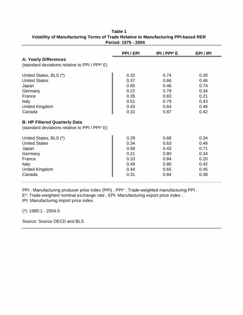
Table 1 Volatility of Manufacturing Terms of Trade Relative to Manufacturing PPI-based RER Period: 1975 - 2004

PPI / EPI IPI / PPI* E EPI / IPIA: Yearly Differences(standard deviations relative to PPI / PPI* E)

United States, BLS (*) 0.32 0.74 0.30United States 0.37 0.66 0.46Japan 0.65 0.46 0.74Germany 0.22 0.79 0.34France 0.35 0.83 0.21Italy 0.51 0.79 0.43United Kingdom 0.43 0.64 0.46Canada 0.31 0.87 0.42

B: HP Filtered Quarterly Data(standard deviations relative to PPI / PPI* E)

United States, BLS (*) 0.29 0.68 0.34United States 0.34 0.63 0.46Japan 0.58 0.43 0.71Germany 0.21 0.80 0.34France 0.33 0.84 0.20Italy 0.49 0.80 0.42United Kingdom 0.44 0.65 0.45Canada 0.31 0.84 0.38

PPI : Manufacturing producer price index (PPI) , PPI* : Trade-weighted manufacturing PPI ,E*: Trade-weighted nominal exchange rate , EPI: Manufacturing export price index ,IPI: Manufacturing import price index.

(*): 1985:1 - 2004:3

Source: Source OECD and BLS

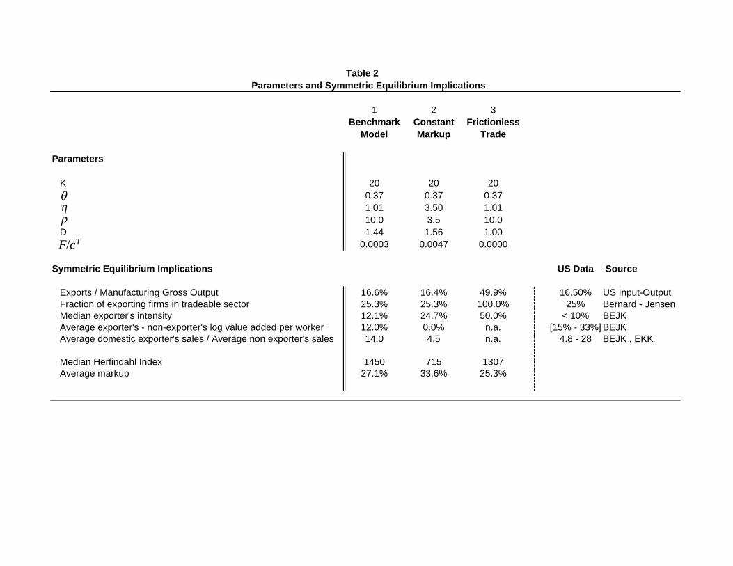
Table 2 Parameters and Symmetric Equilibrium Implications

1 2 3Benchmark Constant Frictionless

Model Markup Trade

Parameters

K 20 20 200.37 0.37 0.371.01 3.50 1.0110.0 3.5 10.0

D 1.44 1.56 1.000.0003 0.0047 0.0000

Symmetric Equilibrium Implications US Data Source

Exports / Manufacturing Gross Output 16.6% 16.4% 49.9% 16.50% US Input-Output Fraction of exporting firms in tradeable sector 25.3% 25.3% 100.0% 25% Bernard - Jensen Median exporter's intensity 12.1% 24.7% 50.0% < 10% BEJK Average exporter's - non-exporter's log value added per worker 12.0% 0.0% n.a. [15% - 33%] BEJK Average domestic exporter's sales / Average non exporter's sales 14.0 4.5 n.a. 4.8 - 28 BEJK , EKK

Median Herfindahl Index 1450 715 1307 Average markup 27.1% 33.6% 25.3%

F/cT

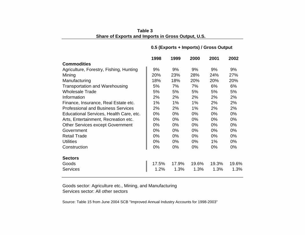
Table 3 Share of Exports and Imports in Gross Output, U.S.

0.5 (Exports + Imports) / Gross Output

1998 1999 2000 2001 2002CommoditiesAgriculture, Forestry, Fishing, Hunting 9% 9% 9% 9% 9%Mining 20% 23% 28% 24% 27%Manufacturing 18% 18% 20% 20% 20%Transportation and Warehousing 5% 7% 7% 6% 6%Wholesale Trade 5% 5% 5% 5% 5%Information 2% 2% 2% 2% 2%Finance, Insurance, Real Estate etc. 1% 1% 1% 2% 2%Professional and Business Services 2% 2% 1% 2% 2%Educational Services, Health Care, etc. 0% 0% 0% 0% 0%Arts, Entertainment, Recreation etc. 0% 0% 0% 0% 0%Other Services except Government 0% 0% 0% 0% 0%Government 0% 0% 0% 0% 0%Retail Trade 0% 0% 0% 0% 0%Utilities 0% 0% 0% 1% 0%Construction 0% 0% 0% 0% 0%

SectorsGoods 17.5% 17.9% 19.6% 19.3% 19.6%Services 1.2% 1.3% 1.3% 1.3% 1.3%

Goods sector: Agriculture etc., Mining, and ManufacturingServices sector: All other sectors

Source: Table 15 from June 2004 SCB "Improved Annual Industry Accounts for 1998-2003"

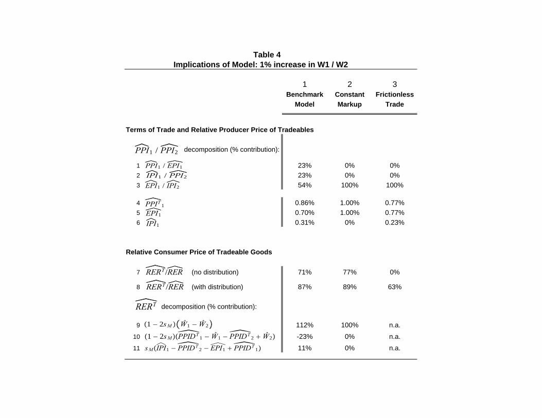
Table 4 Implications of Model: 1% increase in W1 / W2

1 2 3Benchmark Constant Frictionless

Model Markup Trade

Terms of Trade and Relative Producer Price of Tradeables

decomposition (% contribution):

1 23% 0% 0%2 23% 0% 0%3 54% 100% 100%

4 0.86% 1.00% 0.77%5 0.70% 1.00% 0.77%6 0.31% 0% 0.23%

Relative Consumer Price of Tradeable Goods

7 (no distribution) 71% 77% 0%

8 (with distribution) 87% 89% 63%

decomposition (% contribution):

9 112% 100% n.a.

10 -23% 0% n.a.

11 11% 0% n.a.

RERT/RER

PPI1 / EPI1IPI1 / PPI2EPI1 / IPI2

PPI1 / PPI2

RERT

1 − 2sM Ŵ1 − Ŵ2

1 − 2sMPPIDT 1 − Ŵ1 − PPIDT 2 Ŵ2

sMIPI1 − PPIDT 2 − EPI1 PPIDT 1

RERT/RER

PPIT 1

EPI1IPI1

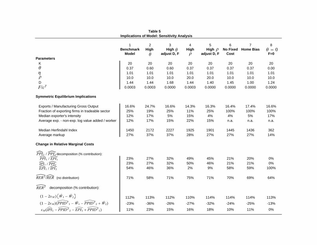
Table 5Implications of Model: Sensitivity Analysis

1 2 3 4 5 6 7 8Benchmark High High High High No Fixed Home Bias

Model adjust D, F adjust D, F Cost F=0Parameters K 20 20 20 20 20 20 20 20

0.37 0.60 0.60 0.37 0.37 0.37 0.37 0.001.01 1.01 1.01 1.01 1.01 1.01 1.01 1.0110.0 10.0 10.0 20.0 20.0 10.0 10.0 10.0

D 1.44 1.44 1.68 1.44 1.40 1.45 1.00 1.240.0003 0.0003 0.0000 0.0003 0.0000 0.0000 0.0000 0.0000

Symmetric Equilibrium Implications

Exports / Manufacturing Gross Output 16.6% 24.7% 16.6% 14.3% 16.3% 16.4% 17.4% 16.6% Fraction of exporting firms in tradeable sector 25% 19% 25% 11% 25% 100% 100% 100% Median exporter's intensity 12% 17% 5% 15% 4% 4% 5% 17% Average exp. - non-exp. log value added / worker 12% 17% 15% 22% 15% n.a. n.a. n.a.

Median Herfindahl Index 1450 2172 2227 1925 1901 1445 1436 362 Average markup 27% 37% 37% 28% 27% 27% 27% 14%

Change in Relative Marginal Costs

decomposition (% contribution):23% 27% 32% 49% 45% 21% 20% 0%23% 27% 32% 50% 46% 21% 21% 0%54% 46% 36% 2% 9% 58% 59% 100%

(no distribution) 71% 58% 71% 75% 71% 70% 69% 64%

decomposition (% contribution):

112% 113% 112% 110% 114% 114% 114% 113%

-23% -36% -26% -27% -32% -24% -25% -13%

11% 23% 15% 16% 18% 10% 11% 0%

F/cT

PPI1 / EPI1IPI1 / PPI2EPI1 / IPI2

PPI1 / PPI2

RERT/RER

RERT

1 − 2sM Ŵ1 − Ŵ2

1 − 2sMPPIDT 1 − Ŵ1 − PPIDT 2 Ŵ2

sMIPI1 − PPIDT 2 − EPI1 PPIDT 1

0

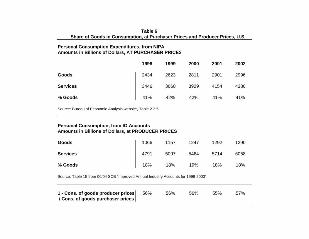
Table 6 Share of Goods in Consumption, at Purchaser Prices and Producer Prices, U.S.

Personal Consumption Expenditures, from NIPA Amounts in Billions of Dollars, AT PURCHASER PRICES

1998 1999 2000 2001 2002

Goods 2434 2623 2811 2901 2996

Services 3446 3660 3929 4154 4380

% Goods 41% 42% 42% 41% 41%

Source: Bureau of Economic Analysis website, Table 2.3.5

Personal Consumption, from IO AccountsAmounts in Billions of Dollars, at PRODUCER PRICES

Goods 1066 1157 1247 1292 1290

Services 4791 5097 5464 5714 6058

% Goods 18% 18% 19% 18% 18%

Source: Table 15 from 06/04 SCB "Improved Annual Industry Accounts for 1998-2003"

1 - Cons. of goods producer prices 56% 56% 56% 55% 57% / Cons. of goods purchaser prices

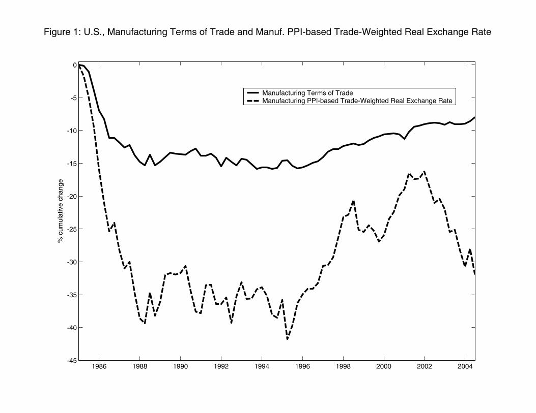
Figure 1: U.S., Manufacturing Terms of Trade and Manuf. PPI-based Trade-Weighted Real Exchange Rate

1986 1988 1990 1992 1994 1996 1998 2000 2002 2004-45

-40

-35

-30

-25

-20

-15

-10

-5

0%

cum

ulat

ive

chan

ge

Manufacturing Terms of TradeManufacturing PPI-based Trade-Weighted Real Exchange Rate

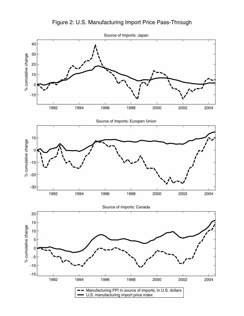
1992 1994 1996 1998 2000 2002 2004-15

-10

-5

0

5

10

15

20

Source of Imports: Canada

% c

umul

ativ

e ch

ange

1992 1994 1996 1998 2000 2002 2004

-30

-20

-10

0

10

Source of Imports: Europen Union

% c

umul

ativ

e ch

ange

Figure 2: U.S. Manufacturing Import Price Pass-Through

1992 1994 1996 1998 2000 2002 2004

-10

0

10

20

30

40

Source of Imports: Japan

% c

umul

ativ

e ch

ange

Manufacturing PPI in source of imports, in U.S. dollarsU.S. manufacturing import price index

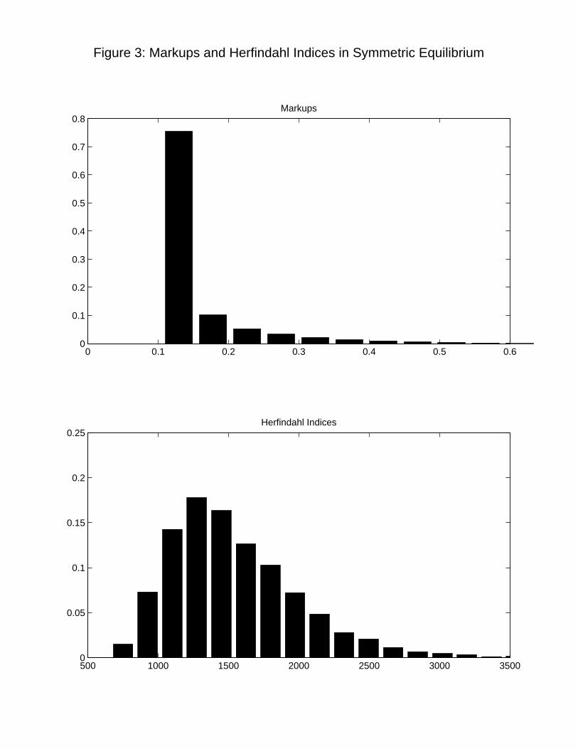
0 0.1 0.2 0.3 0.4 0.5 0.60

0.1

0.2

0.3

0.4

0.5

0.6

0.7

0.8Markups

Figure 3: Markups and Herfindahl Indices in Symmetric Equilibrium

500 1000 1500 2000 2500 3000 35000

0.05

0.1

0.15

0.2

0.25Herfindahl Indices

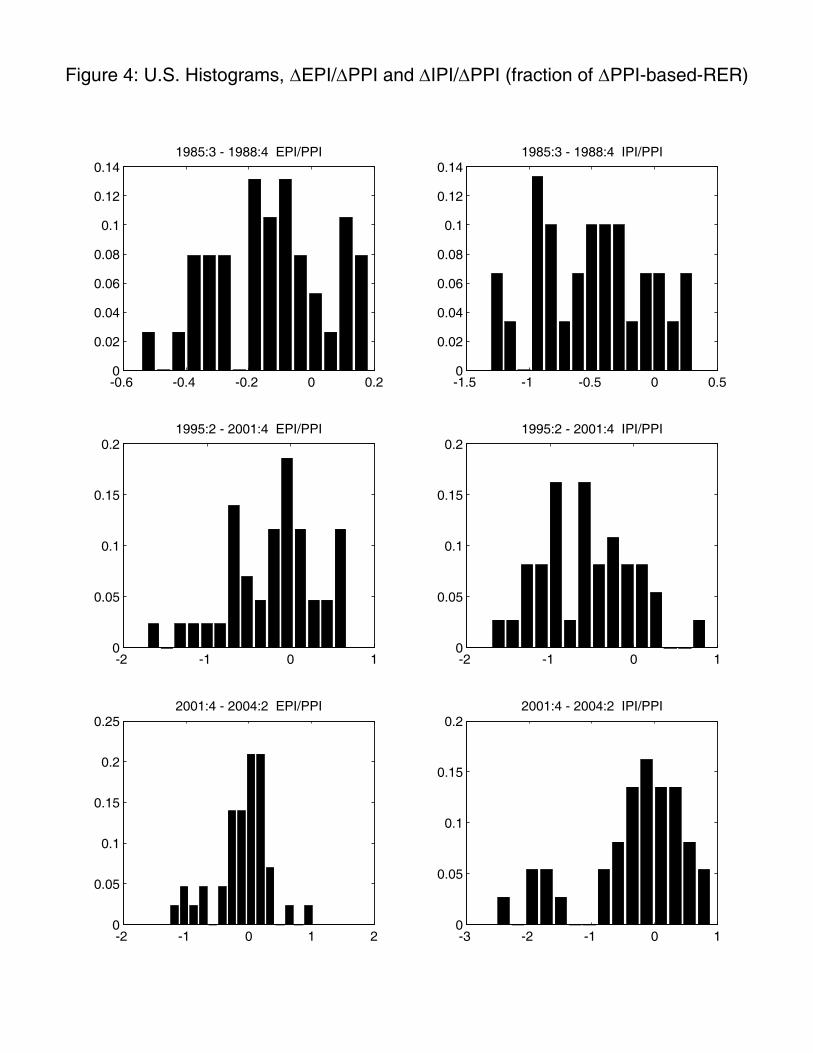
-0.6 -0.4 -0.2 0 0.20

0.02

0.04

0.06

0.08

0.1

0.12

0.141985:3 - 1988:4 EPI/PPI

-1.5 -1 -0.5 0 0.50

0.02

0.04

0.06

0.08

0.1

0.12

0.141985:3 - 1988:4 IPI/PPI

-2 -1 0 10

0.05

0.1

0.15

0.21995:2 - 2001:4 EPI/PPI

-2 -1 0 10

0.05

0.1

0.15

0.21995:2 - 2001:4 IPI/PPI

-2 -1 0 1 20

0.05

0.1

0.15

0.2

0.252001:4 - 2004:2 EPI/PPI

Figure 4: U.S. Histograms, ∆EPI/∆PPI and ∆IPI/∆PPI (fraction of ∆PPI-based-RER)

-3 -2 -1 0 10

0.05

0.1

0.15

0.22001:4 - 2004:2 IPI/PPI

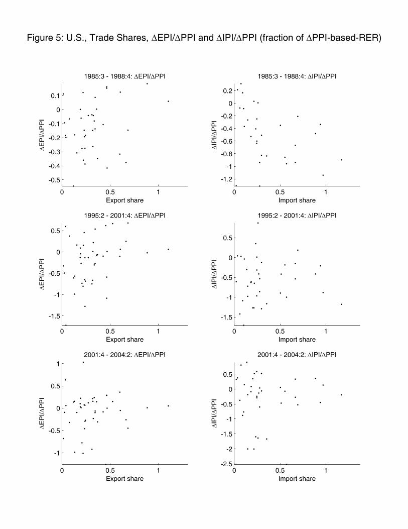
0 0.5 1

-1

-0.5

0

0.5

12001:4 - 2004:2: ∆EPI/∆PPI

Export share

∆E

PI/∆

PP

I

0 0.5 1-2.5

-2

-1.5

-1

-0.5

0

0.5

2001:4 - 2004:2: ∆IPI/∆PPI

Import share

∆IP

I/∆P

PI

0 0.5 1

-1.5

-1

-0.5

0

0.5

1995:2 - 2001:4: ∆EPI/∆PPI

Export share

∆E

PI/∆

PP

I

0 0.5 1

-1.5

-1

-0.5

0

0.5

1995:2 - 2001:4: ∆IPI/∆PPI

Import share

∆IP

I/∆P

PI

0 0.5 1

-0.5

-0.4

-0.3

-0.2

-0.1

0

0.1

1985:3 - 1988:4: ∆EPI/∆PPI

Export share

∆E

PI/∆

PP

IFigure 5: U.S., Trade Shares, ∆EPI/∆PPI and ∆IPI/∆PPI (fraction of ∆PPI-based-RER)

0 0.5 1

-1.2

-1

-0.8

-0.6

-0.4

-0.2

0

0.2

1985:3 - 1988:4: ∆IPI/∆PPI

Import share

∆IP

I/∆P

PI

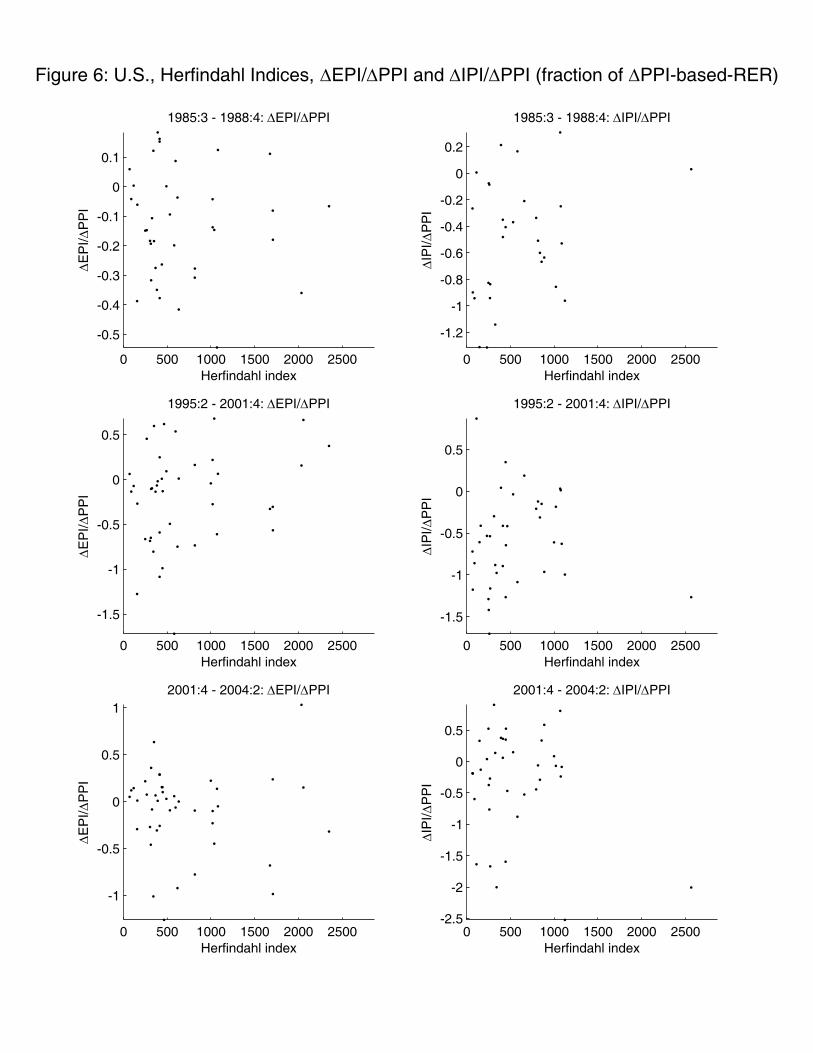
0 500 1000 1500 2000 2500

-1

-0.5

0

0.5

12001:4 - 2004:2: ∆EPI/∆PPI

Herfindahl index

∆E

PI/∆

PP

I

0 500 1000 1500 2000 2500-2.5

-2

-1.5

-1

-0.5

0

0.5

2001:4 - 2004:2: ∆IPI/∆PPI

Herfindahl index

∆IP

I/∆P

PI

0 500 1000 1500 2000 2500

-1.5

-1

-0.5

0

0.5

1995:2 - 2001:4: ∆EPI/∆PPI

Herfindahl index

∆E

PI/∆

PP

I

0 500 1000 1500 2000 2500

-1.5

-1

-0.5

0

0.5

1995:2 - 2001:4: ∆IPI/∆PPI

Herfindahl index

∆IP

I/∆P

PI

0 500 1000 1500 2000 2500

-0.5

-0.4

-0.3

-0.2

-0.1

0

0.1

1985:3 - 1988:4: ∆EPI/∆PPI

Herfindahl index

∆E

PI/∆

PP

IFigure 6: U.S., Herfindahl Indices, ∆EPI/∆PPI and ∆IPI/∆PPI (fraction of ∆PPI-based-RER)

0 500 1000 1500 2000 2500

-1.2

-1

-0.8

-0.6

-0.4

-0.2

0

0.2

1985:3 - 1988:4: ∆IPI/∆PPI

Herfindahl index

∆IP

I/∆P

PI

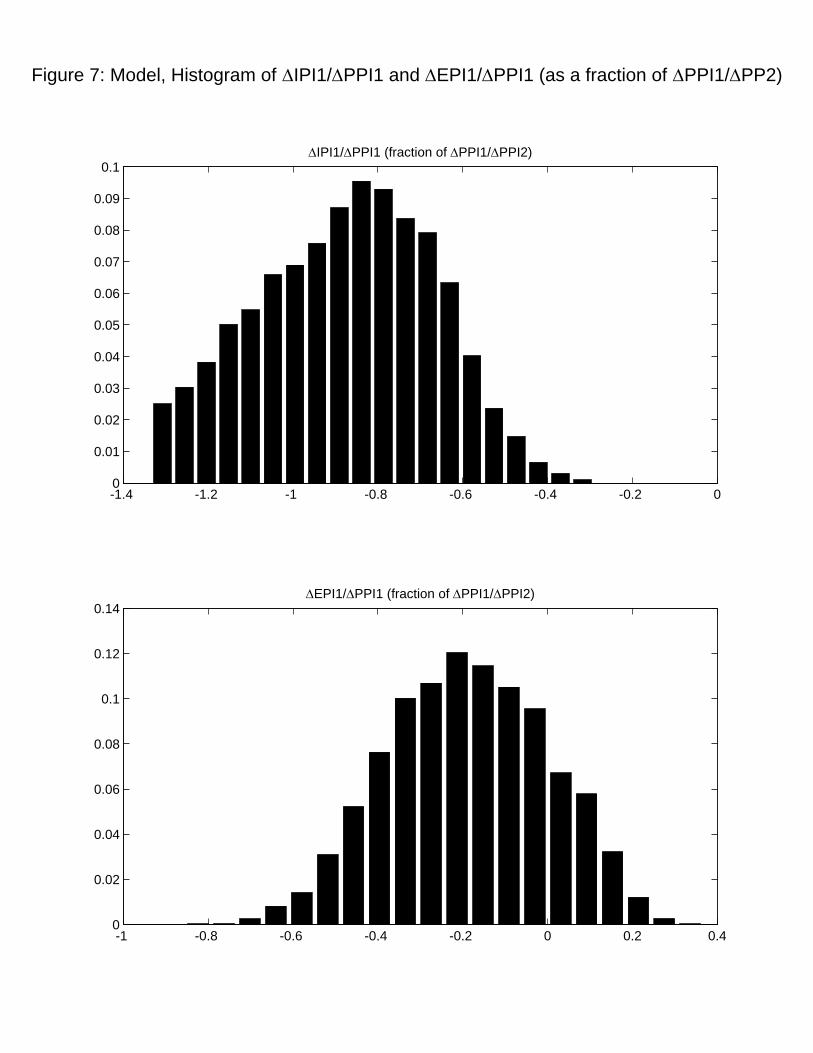
-1.4 -1.2 -1 -0.8 -0.6 -0.4 -0.2 00

0.01

0.02

0.03

0.04

0.05

0.06

0.07

0.08

0.09

0.1∆IPI1/∆PPI1 (fraction of ∆PPI1/∆PPI2)

Figure 7: Model, Histogram of ∆IPI1/∆PPI1 and ∆EPI1/∆PPI1 (as a fraction of ∆PPI1/∆PP2)

-1 -0.8 -0.6 -0.4 -0.2 0 0.2 0.40

0.02

0.04

0.06

0.08

0.1

0.12

0.14∆EPI1/∆PPI1 (fraction of ∆PPI1/∆PPI2)