Trade Costs and Puzzles in International … International Journal of Applied Economics, 8(2), September 2011, 18-42 18 Trade Costs and Puzzles in International Macroeconomics Luke

Willard, International Journal of Applied Economics, 8(2), September 2011, 18-42 18

Trade Costs and Puzzles in International Macroeconomics

Luke Willard

Australian Government Treasury

Abstract: Obstfeld and Rogoff (2001) argue that trade costs provide at least part of the explanation for a number of puzzles in international macroeconomics. Using data on imports to the United States from developed economies, this paper investigates whether trade costs are related to correlations associated with three of these puzzles: the Feldstein-Horioka saving-investment puzzle, the purchasing power parity real exchange rate persistence puzzle and the international consumption correlation puzzle. There is evidence in support of trade costs playing a role in the Feldstein-Horioka puzzle.

Keywords: Consumption smoothing, Feldstein-Horioka puzzle, Purchasing power puzzle, Trade JEL Classification: F3, F4

1. Introduction

The international macroeconomics literature has identified a number of key empirical correlations, which are often described as puzzles because of their apparent inconsistency with theory. One, called the Feldstein-Horioka puzzle, is why domestic investment is correlated with domestic saving when, in a world with open capital markets, saving should flow to countries with the greatest investment opportunities. For example, in the sample of developed economies used in this paper there is a correlation between annual saving and investment of 0.36 when theory would predict a low correlation.1 Another, called the purchasing power parity (PPP) puzzle, is associated with why the real exchange rate is very persistent despite the relative flexibility implied by high nominal exchange rate volatility. For example, Froot and Rogoff (1995) find that it takes over 4 years for a deviation from purchasing power parity to be reduced by one-half in developed economies.2 A third puzzle, called the international consumption correlation puzzle, is why in a world of international trade and capital flows, financial instruments (or other mechanisms) have not developed so as to better help consumption smoothing in the face of country-specific shocks. Some theories suggest that countries should smooth consumption such that every country’s consumption is perfectly correlated with world consumption.3


In a seminal paper in international macroeconomics, Obstfeld and Rogoff (2001) argue that trade costs could explain these puzzles (as well as some other puzzles such as the extent of the bias toward domestic shares in equity portfolios). This paper seeks to assess the extent to which the data suggest that trade costs can explain the Feldstein-Horioka, purchasing power parity and international consumption correlation puzzles.

While many papers have been written seeking to explain why the empirical regularities studied here should not be viewed as puzzles, the existence of papers like Obstfeld and Rogoff (2001) and other works in the field provide evidence that a convincing explanation has yet to be developed for these regularities and hence they still can be viewed as puzzles. For example, Baxter and Crucini (1993) could be viewed as providing an explanation of the saving-investment correlation. However the explanation does not seem perfectly satisfactory as the model also predicts that consumption should be nearly perfectly correlated across countries. Hence an approach like the one adopted here of examining how much a single factor explains a number of features of the data is appealing. Similarly Kehoe and Perri (2002) explain a number of puzzles through incomplete markets but introduce others. The research presented here is complementary to this earlier work, as it examines the role of another factor, trade costs, and also, later, examines the robustness of the results when a measure of financial restrictions is included in the analysis. In addition, whether or not the empirical regularities are strictly viewed as puzzles, better understanding factors related to their existence is of interest from policy making and forecasting perspectives as well as in assessing how well theories explain features of the data.

In essence Obstfeld and Rogoff suggest that trade costs for goods can cause phenomena that are similar to financial market imperfections, which are natural explanations for both the Feldstein-Horioka and consumption correlation puzzles. One simple example of how trade costs can introduce financial imperfections involves a small economy, where the rest of the world has a real interest rate and no inflation. In the first period suppose that the small economy imports some of its consumption. Hence the economy must export some of its produce in the second period to satisfy its budget constraint. So this means that prices will be higher in period 1 than in period 2, as in the first period home prices must be higher than the foreign price of the good while in the second period it must be lower. This will result in an expected deflation and the small economy’s real interest rate will be above the world real interest rate. So the trade cost causes a wedge between real interest rates in the small economy and the rest of the world. This shows that price wedges can cause wedges in real interest rates between countries. Fazio et al. (2005) also suggest that trade costs can explain the Feldstein-Horioka puzzle because of the differential between consumption and output


prices. Either way there are theories that trade costs can explain the puzzles thus providing motivation for the empirical approach of this paper.

With financial market imperfections, global saving do not necessarily flow to the most profitable investments, which would explain the high correlation of domestic saving and investment. Similarly financial market imperfections due to trade costs also lessen the extent of consumption smoothing across countries. Trade costs also explain why the same good may not cost the same amount in different countries and so provides a natural explanation of deviations from purchasing power parity (see the discussion in Dumas, 1992).4 (More detailed explanations for the role of trade costs in these puzzles can be found in Obstfeld and Rogoff (2001).)

The contribution of this paper is to empirically assess the plausibility of the trade cost explanation for these three puzzles within a simple framework, which is applied across each of the puzzles. Even if one is uncomfortable characterizing the correlations discussed in this paper as puzzles, this paper can be viewed as an attempt to see whether certain aspects of the correlations can be accounted for by trade costs for the purposes of better understanding and predicting economic developments.

Some existing literature looks at whether trade costs can explain the potentially related puzzle of the home bias in portfolio holdings (Coeurdacier, 2008, and van Wincoop and Warnock, 2010). Other work has found evidence between the home bias in portfolio holdings and the international consumption correlation puzzle (Sørensen et al, 2007). Other related literature looks at the channels of consumption smoothing (such as Asdrubali et al, 1996). Ghironi and Melitz (2005) also develop a general equilibrium model which sheds light on some of these puzzles using a calibrated measure of trade cost (rather than actual data). This paper is very much complementary to this existing research.

Determining the extent to which trade costs might explain these three puzzles in macroeconomics would be important in a number of respects. It would aid in the prediction of and interpretation of movements in the real exchange rate, investment and consumption. For example, if trade costs continue to decline and trade costs play a role in these puzzles it would be expected that real exchange rates would tend to adjust to shocks more quickly, domestic investment and saving would become less closely related and consumption would become less related to domestic output growth. It is also likely to change the way in which shocks that influence the real exchange rate impact on the rest of the economy.


If there is evidence that trade costs explain the consumption correlation puzzle, it would suggest that lower trade costs can raise welfare by enabling better consumption smoothing (in addition to the conventional greater opportunities to benefit from comparative advantage). Similarly if trade costs explain the Feldstein-Horioka puzzle, it suggests that lowering trading costs will help saving flow to where investment returns are higher.

To preview the results, there is some evidence that trade costs (which in this paper are generally measured as the average percentage trade cost including insurance, freight and duties) play a role in the Feldstein-Horioka puzzle for the developed economies in the sample. However it appears to play a small role, if any, in the PPP and consumption correlation puzzles.

In Section 2, the main empirical methods used are described. Section 3 presents the data and the main results. Section 4 includes some results examining whether capital restrictions play a role. Section 5 presents results using an alternative measure of trade costs and some additional checks of robustness. Section 6 discusses in more detail what aspects of the correlations trade costs appear to account for and a brief conclusion appears in Section 7.

2. Method

Obstfeld and Rogoff (2001) present a series of simple models using trade cost (where a percentage of the good is lost in transport) to argue that trade costs can explain these three puzzles. The estimation approach used in this paper uses panel data (across countries and time) to examine the link between trade costs and various measures of the extent of these puzzles (for example, a higher correlation between saving and investment for the Feldstein-Horioka puzzle).

The approach involves running regressions similar to those seen in the existing literature about these puzzles but also including terms relating to trade costs, which are proxied by cost data based on US imports. These data are used because firstly they seem to be close to what Rogoff and Obstfeld’s model suggests is most relevant (costs that cause a wedge between prices faced by locals and foreigners). Secondly they are one of the few reliable sources for trade costs (Hummels and Lugovskyy, 2006).

To examine whether trade costs play a role in the Feldstein-Horioka puzzle, variations of the following regression are run on data from 1974-2006:


itititit

it

it

iti

it

it effYS

YS

YI

11111 ++++= θγφδ (1)

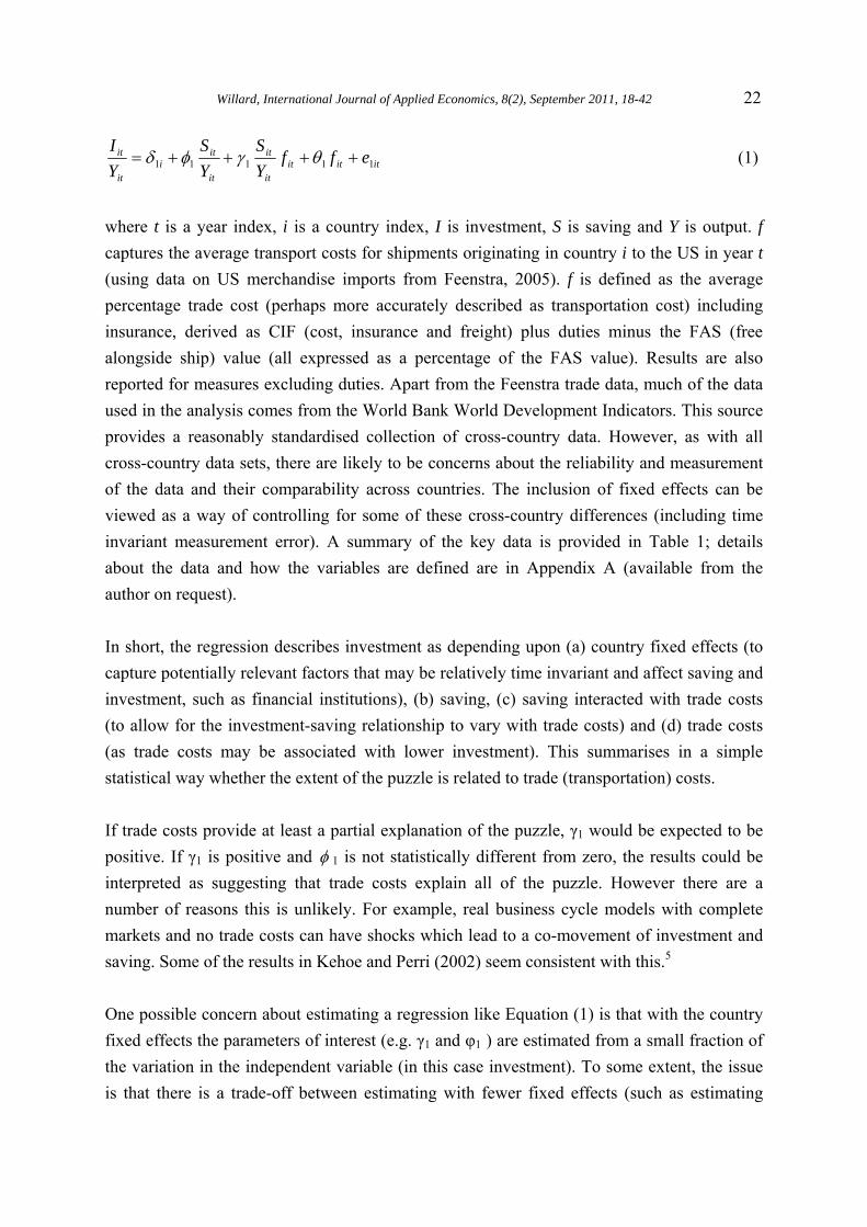
where t is a year index, i is a country index, I is investment, S is saving and Y is output. f captures the average transport costs for shipments originating in country i to the US in year t (using data on US merchandise imports from Feenstra, 2005). f is defined as the average percentage trade cost (perhaps more accurately described as transportation cost) including insurance, derived as CIF (cost, insurance and freight) plus duties minus the FAS (free alongside ship) value (all expressed as a percentage of the FAS value). Results are also reported for measures excluding duties. Apart from the Feenstra trade data, much of the data used in the analysis comes from the World Bank World Development Indicators. This source provides a reasonably standardised collection of cross-country data. However, as with all cross-country data sets, there are likely to be concerns about the reliability and measurement of the data and their comparability across countries. The inclusion of fixed effects can be viewed as a way of controlling for some of these cross-country differences (including time invariant measurement error). A summary of the key data is provided in Table 1; details about the data and how the variables are defined are in Appendix A (available from the author on request).

In short, the regression describes investment as depending upon (a) country fixed effects (to capture potentially relevant factors that may be relatively time invariant and affect saving and investment, such as financial institutions), (b) saving, (c) saving interacted with trade costs (to allow for the investment-saving relationship to vary with trade costs) and (d) trade costs (as trade costs may be associated with lower investment). This summarises in a simple statistical way whether the extent of the puzzle is related to trade (transportation) costs.

If trade costs provide at least a partial explanation of the puzzle, γ1 would be expected to be positive. If γ1 is positive and φ 1 is not statistically different from zero, the results could be interpreted as suggesting that trade costs explain all of the puzzle. However there are a number of reasons this is unlikely. For example, real business cycle models with complete markets and no trade costs can have shocks which lead to a co-movement of investment and saving. Some of the results in Kehoe and Perri (2002) seem consistent with this.5

One possible concern about estimating a regression like Equation (1) is that with the country fixed effects the parameters of interest (e.g. γ1 and φ1 ) are estimated from a small fraction of the variation in the independent variable (in this case investment). To some extent, the issue is that there is a trade-off between estimating with fewer fixed effects (such as estimating


with just country fixed effects) and estimating with more fixed effects (such as with country-decade fixed effects). The former approach may reduce the extent of multicollinearity and is likely to be more informative as it estimates less parameters from the same number of observations (assuming the equations are not mis-specified). The later is likely to be more immune from arguments that other factors not included in the regression could explain the apparent correlation between saving and investment.

Comparisons are made of the results from regression (1) to those of the regression excluding the interaction and trade cost terms. If trade costs can account for much of the puzzle, the coefficient on investment should be much smaller in regression (1) than in the regression without trade cost terms.

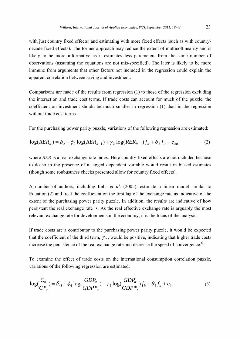
For the purchasing power parity puzzle, variations of the following regression are estimated:

itititititit effRERRERRER 2212122 )log()log()log( ++++= −− θγφδ (2)

where RER is a real exchange rate index. Here country fixed effects are not included because to do so in the presence of a lagged dependent variable would result in biased estimates (though some roubustness checks presented allow for country fixed effects).

A number of authors, including Imbs et al. (2005), estimate a linear model similar to Equation (2) and treat the coefficient on the first lag of the exchange rate as indicative of the extent of the purchasing power parity puzzle. In addition, the results are indicative of how persistent the real exchange rate is. As the real effective exchange rate is arguably the most relevant exchange rate for developments in the economy, it is the focus of the analysis.

If trade costs are a contributor to the purchasing power parity puzzle, it would be expected that the coefficient of the third term, 2γ , would be positive, indicating that higher trade costs increase the persistence of the real exchange rate and decrease the speed of convergence.6

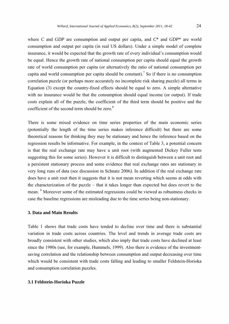
To examine the effect of trade costs on the international consumption correlation puzzle, variations of the following regression are estimated:

itititt

it

t

iti

t

it effGDPGDP

GDPGDP

CC

44444 )*

log()*

log()*

log( ++++= θγφδ (3)


where C and GDP are consumption and output per capita, and C* and GDP* are world consumption and output per capita (in real US dollars). Under a simple model of complete insurance, it would be expected that the growth rate of every individual’s consumption would be equal. Hence the growth rate of national consumption per capita should equal the growth rate of world consumption per capita (or alternatively the ratio of national consumption per capita and world consumption per capita should be constant).7 So if there is no consumption correlation puzzle (or perhaps more accurately no incomplete risk sharing puzzle) all terms in Equation (3) except the country-fixed effects should be equal to zero. A simple alternative with no insurance would be that the consumption should equal income (or output). If trade costs explain all of the puzzle, the coefficient of the third term should be positive and the coefficient of the second term should be zero.8

There is some mixed evidence on time series properties of the main economic series (potentially the length of the time series makes inference difficult) but there are some theoretical reasons for thinking they may be stationary and hence the inference based on the regression results be informative. For example, in the context of Table 3, a potential concern is that the real exchange rate may have a unit root (with augmented Dickey Fuller tests suggesting this for some series). However it is difficult to distinguish between a unit root and a persistent stationary process and some evidence that real exchange rates are stationary in very long runs of data (see discussion in Schnatz 2006). In addition if the real exchange rate does have a unit root then it suggests that it is not mean reverting which seems at odds with the characterization of the puzzle – that it takes longer than expected but does revert to the mean. 9 Moreover some of the estimated regressions could be viewed as robustness checks in case the baseline regressions are misleading due to the time series being non-stationary.

3. Data and Main Results

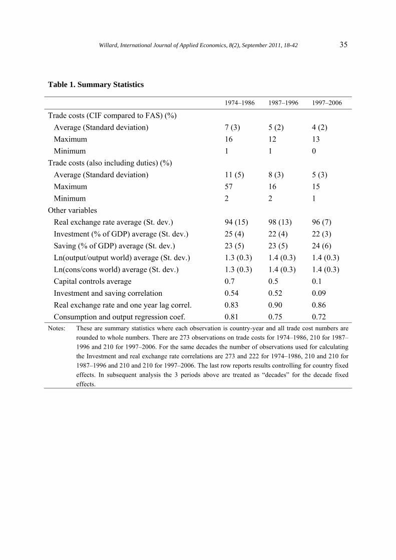
Table 1 shows that trade costs have tended to decline over time and there is substantial variation in trade costs across countries. The level and trends in average trade costs are broadly consistent with other studies, which also imply that trade costs have declined at least since the 1980s (see, for example, Hummels, 1999). Also there is evidence of the investment-saving correlation and the relationship between consumption and output decreasing over time which would be consistent with trade costs falling and leading to smaller Feldstein-Horioka and consumption correlation puzzles.

3.1 Feldstein-Horioka Puzzle


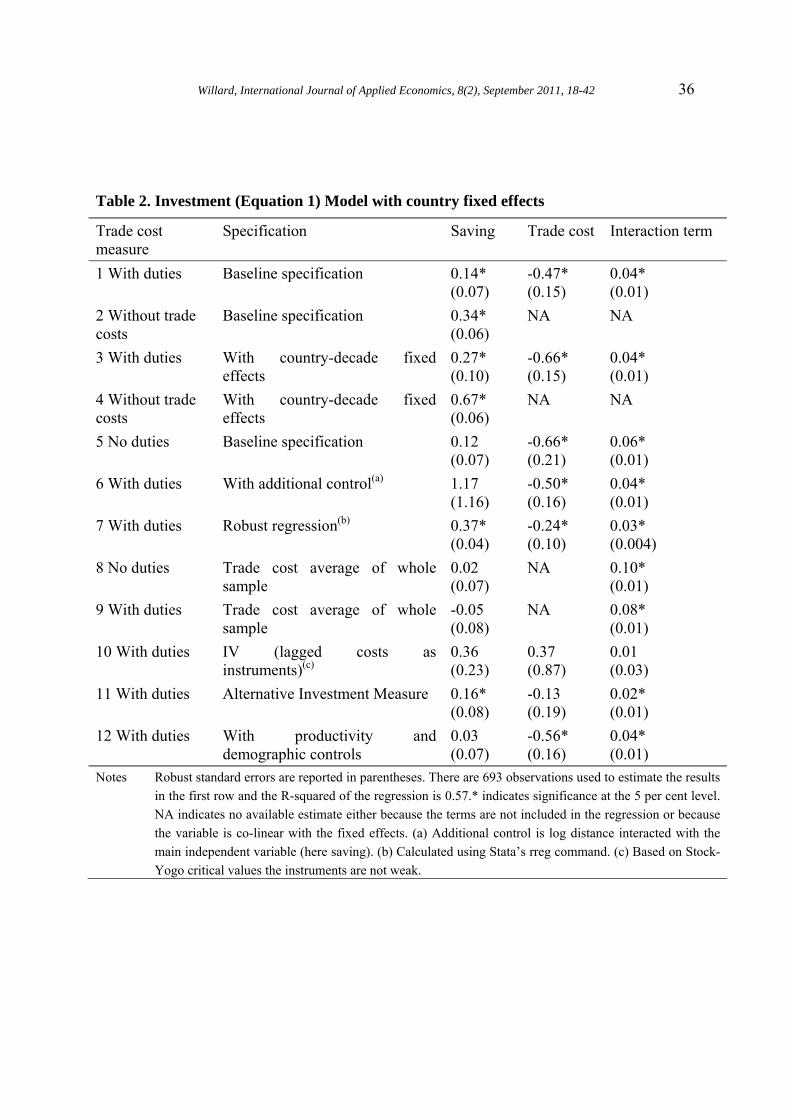
Table 2 reports the estimates for the investment equation (which sheds light on the Feldstein-Horioka puzzle). Each row reports the coefficients from a single regression; results for a wide variety of specification and samples are reported, providing evidence of the robustness of the results.

Proceeding from the top of Table 2, the first two regressions reported are the focus of the analysis. The first regression estimates Equation (1) with trade cost terms (including duties) while the second regression excludes trade costs. With trade costs, the interaction term (last column) is positive and significant though the saving coefficient is not zero, suggesting that trade costs are only a partial explanation of the puzzle. In particular it suggests that even if trade costs were equal to zero there would be a relationship between investment and saving. The extent to which trade costs can account for the puzzle is indicated by the lower coefficient on saving in the model with trade costs compared to the coefficient without them (first column, row 1’s 0.14 versus row 2’s 0.34). Also the coefficient on trade cost is negative and significant (row 1 middle column) and the R-squared reported in the notes indicates that the regression explains a reasonable amount of the variation in investment.

Results for a variety of potentially reasonable alternative specifications are as follows. The third and fourth regressions include country-decade fixed effects (which can lead to better estimates if it is believed that the relationship between investment and saving may vary within the same country over time say because of productivity shocks or demographics). As the theory only describes trade costs in a simple way it is reassuring that the results estimated using this regression are similar to those in the first two row. The fifth row reports the results where the trade cost measure does not include duties. The results are similar to the first row.

The sixth regression is estimated with log distance (from the US) interacted with the main independent variable included in the regression (here saving), as well as the standard monetary measure of trade costs. This is designed to examine whether the results are sensitive to the inclusion of other variables that may measure trade costs (at least with the largest economy in the world). One motivation for including this variable is to examine whether the main trade cost variable may be picking up the effects of trade costs specific to the US. It is notable that the trade cost(based on CIF and FAS data)-saving interaction term remains positive and significant (suggesting monetary trade costs play a role). However the coefficient on saving becomes larger (though it is statistically indistinguishable from zero). This regression could be interpreted as suggesting that once a rich enough set of trade cost measures are included, the positive correlation between saving and investment disappears.


The seventh regression reports the results using a robust regression procedure which seeks to down play the role of potential outliers. This regression has similar results to the baseline specification, though the coefficient on saving is larger. Rows eight and nine report the results of using average trade costs over the sample as the measure of trade cost. This could help eliminate measurement error and so may yield better estimates. Consistent with this, the estimate on the interaction term is larger in this specification, at least compared to the baseline specification and in this specification the saving term becomes insignificant and small.

The tenth row reports the results using instrumental variables (IV), where the lagged trade costs is used as an instrument. IV estimation is motivated as the trade cost measure provides a noisy measure of the actual trade cost. However, the standard errors are large (as is common with IV estimation) suggesting this method does not provide very informative results. The eleventh row reports results using an alternative measure of investment (using gross fixed capital formation instead of gross capital formation) and including productivity (GDP). The twelfth row reports results with demographic and productivity controls. The latter is motivated by Taylor (1994) who finds evidence that demographic and productivity changes account for some of the puzzle consistent with demographic and productivity changes affecting both investment and saving.10

In summary, the regression results in Table 2 generally suggest that there is evidence that increased trade costs are associated with a bigger correlation between investment and saving (as indicated by the tendency for the coefficient on the interaction variable to be positive and significant). Even so, trade costs can explain some, but generally not all of the Feldstein-Horioka puzzle since the coefficient on saving tends to be typically lower in the model with transaction costs than the one without, though it remains positive and significant.

3.2 PPP Puzzle

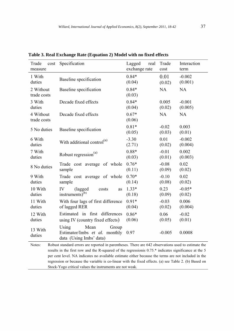
Table 3 presents estimates from a similar set of regressions with the real exchange rate as the dependent variable and the lagged exchange rate as the main independent variable. They show that the coefficients for the trade cost and trade cost interaction term is only sometimes of the correct sign (positive) and generally insignificant. It is noticeable that the lagged real exchange rate coefficient is somewhat smaller compared to models without trade costs. The coefficient estimates from the first row of Table 3 imply that if trade costs were to fall to zero, the half-life of real exchange rates would remain fairly constant at about 4 years.


The last two rows of Table 3 present results that use some alternative estimation methods and/or data that has been used in the existing literature. These rows present the results of approaches which allow for country fixed effects, while attempting to address concerns about endogeneity in dynamic models. Specifically row 12 reports results controlling for country fixed effects by taking first differences and using instruments, which should provide reliable inference. Row 13 uses a mean group estimator and bilateral monthly real exchange rate data between the US and some European countries where prices are particular subcomponents of the CPI index. This is designed to address the concern that the purchasing power parity puzzle is an artefact of using aggregated prices as well as endogeneity concerns (see Imbs et al, 2005).11 It can be see that the last two rows suggest that the exchange rate is highly persistent and also suggest trade costs do not play a major role in this puzzle.

3.3 International Consumption Correlation Puzzle

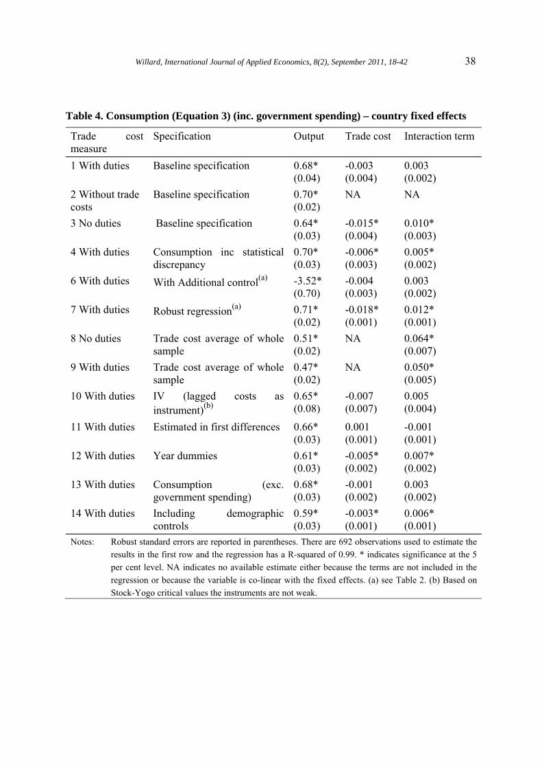
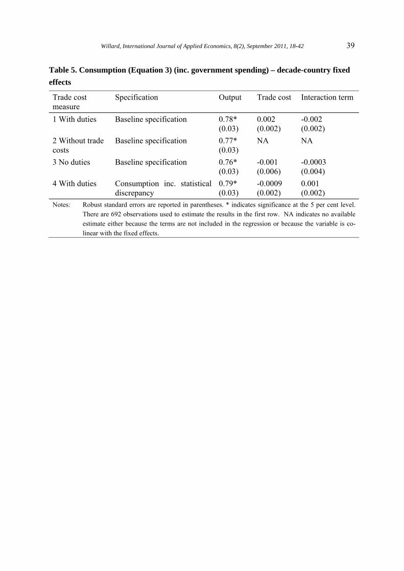
Tables 4 and 5 provide evidence about whether trade costs play a role in the international consumption correlation puzzle.12 Table 4 uses only country fixed effects (that is, it estimates Equation (3), the preferred specification) while Table 5 includes decade-country interactions. Both Tables 4 and 5 report in one row the results with consumption including the statistical discrepancy in case some hard to estimate components of consumption are in the discrepancy. Row 12 of Table 4 reports the regression excluding government spending. The last regression in Table 4 is similar to Townsend (1994) which includes demographic controls. The results from these regressions can be viewed as further robustness checks.

Tables 4 and 5 generally report an interaction coefficient which is positive, though sometimes insignificant. In general, the introduction of the trade cost terms do not substantially change the size of the coefficient on output term suggesting that trade costs do not play a big part in the consumption correlation puzzle. This might be because nontradeables play an important part in the apparent puzzle. This would lead to a correlation between domestic consumption and output. The coefficient on trade costs suggests that higher trade costs are associated with lower consumption. The estimates for the interactive coefficient using trade costs averaged over the whole sample (which may eliminate measurement error) tend to be positive, significant and are larger than the estimates obtained using other regressions. Also it can be seen from the results reported in Table 4 that the results do not seem sensitive to whether consumption includes government spending or not. This suggests that government spending does not play a major role in reducing the consumption correlation puzzle.


In Tables 2-3, it is noticeable that when an additional control is included (that is, the inclusion of an interaction term between the main independent variable and log distance from the US) the main independent variable becomes insignificant and/or negative. As log distance is a measure of trade costs, this could be viewed as suggesting that with a richer or more complete set of measures of trade costs, the apparent Feldstein-Horioka and PPP puzzles can be explained.

As a further robustness check, variants without country fixed effects were estimated, reflecting one possible view that cross-country variation is important and meaningful for understanding the puzzles. They also indicated that the interaction coefficient was positive for the investment regressions (though not the others).

4. Capital Controls

Another potential explanation for the three puzzles could be capital market restrictions. Lewis (1996) argued that such restrictions could explain the lack of consumption risk sharing and Kehoe and Perri (2002) and Engel (2000) suggest that some of the puzzles may be explained by allowing for financial market imperfections. The following regression explores whether capital market restrictions could play a role together with trade costs in explaining the Feldstein-Horioka puzzle:

itit

itit

it

itititititititit

it

it

it

iti

it

it eYS

KYS

fKfKKffYS

YS

YI

143211111 ++++++++= ϖϖϖϖθγφδ (4)

where K is a dummy variable equal to 1 when a country has capital controls and zero otherwise (based on IMF data up to 2005). If the puzzle is due to an interaction of the role of trade costs and capital controls then it would be expected that the interaction coefficient, 3ϖ would be positive. As can be seen from Table 1, many countries removed capital controls during the sample with around 80 percent of observations having capital controls early in the sample but only about 10 percent towards the end.

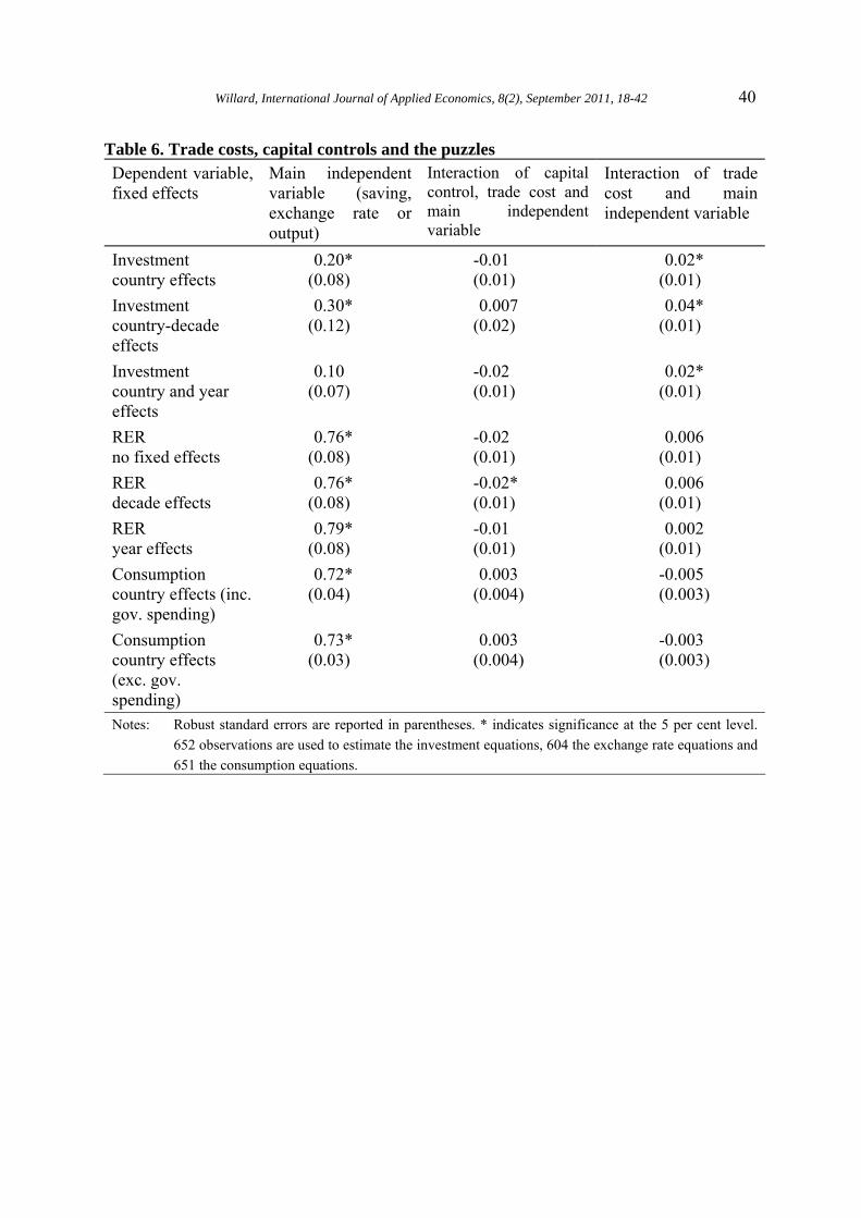
Table 6 presents the results of the real exchange rate, investment and consumption equations using a variety of specifications. The middle column reports the coefficient 3ϖ in Equation (4) or its analogue while the last column reports the coefficient 1γ or its analogue. The coefficient on the main independent variable (saving, the lag of the real exchange rate or output) appears on the left hand side and tends to be positive and significant suggesting that a puzzle still exists even after controlling for trade costs and capital controls. The coefficient


1γ is still positive and significant for the investment equation, indicating that even in the absence of capital controls, trade costs still appear to play a role in explaining the first puzzle. The coefficient is positive but insignificant for the real exchange rate equation and negative and insignificant for the consumption equation.

5. Further Robustness Checks

In this section a number of further checks of the robustness of the results are examined. First a different measure of trade costs is obtained by running the following regression:

kitiskkitf εβα ++= (5)

where f captures the average transport costs for shipments originating in country i to the US of good k. Here goods are aggregated to the 3-digit level in year t (again using Feenstra’s data that is reported using the Standard International Trade Classification revision 2). The βs are allowed to vary across countries and decades (which are indicated with the subscript s) and provide estimates of the transport costs for each country and over time.

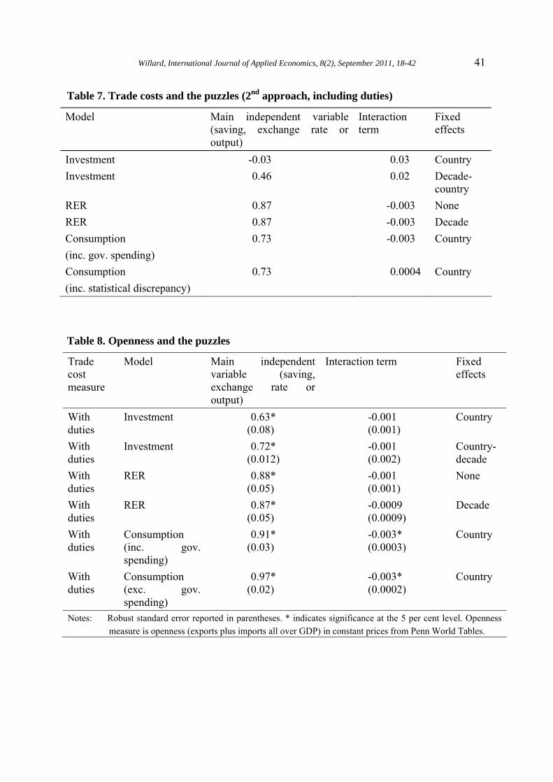
The regression attributes some of the trade cost to a commodity specific effect (as some goods are likely to be more expensive to transport than others) while allowing there to be an effect that varies across time and across countries (represented by the betas) which captures in some sense the underlying transaction costs for the country. While this is a direct and intuitive way of attempting to calculate transportation costs, there are a number of reasons why it may be problematic. For example, it assumes a specific, though not implausible, functional form assumption. However Appendix B (available on request) provides some evidence that this trade cost measure may be reasonable. The results from using this alternative measure of trade costs in Equations (1) to (3) are reported in Table 7. The table provides support for the trade cost explaining the Feldstein-Horioka puzzle. The interaction term is similar in magnitude to estimates seen previously.

Up to this point trade cost measures with the United States have been used as the proxy for general trade costs (largely due to data availability and reliability). To assess if the results are affected by their reliance on US import costs, the extent of trade (as a share of GDP) is used instead of trade costs in Table 8. This approach assumes that higher trade costs are likely to be reflected in lower openness and so openness may be a good and more broadly based indicator of trade costs. In addition this robustness test can lessen concern that the above


results capture the effects of remoteness from the US, the most financially developed country, rather than the effect of trade costs.

Table 8 provides support to trade costs explaining part of the puzzles, including the PPP and consumption puzzles. The results indicate that the more open the economy (which is likely to be associated with lower trade costs) the less extreme the puzzle (as the interaction term is negative) though only for the consumption equations is the interaction term significant.

6. What Aspects of the Puzzles Do the Trade Costs Explain?

The above results suggest that it is possible to find at least some evidence that trade costs are associated with correlations that have been linked with three puzzles in international macroeconomics though the evidence is most strong for the Feldstein-Horioka puzzle. Important issues are whether (a) trade costs can account for much of these correlations and (b) there are only certain aspects of the correlations that trade costs account for or explain.

The first issue can be addressed by comparing the coefficient on the main independent variable in the models with and without trade costs controls. The correlation (or more precisely the regression coefficient) between saving and investment in the data (controlling only for fixed effects) is 0.34 but after also controlling for trade costs this correlation falls to 0.14. This suggests that trade costs can account for over half of the puzzle. For the real exchange rate, the estimates suggest that accounting for trade costs does not reduce the correlation with the lagged real exchange rate. The coefficient estimates imply that if trade costs were to fall to zero, the half-life of real exchange rates would be steady at about 4 years. Trade costs appear to explain little of the consumption correlation puzzle with the preferred specification suggesting that accounting for trade costs has no effect on the correlation between a country’s relative consumption and its relative output, with the correlation remaining stable at about 0.7.

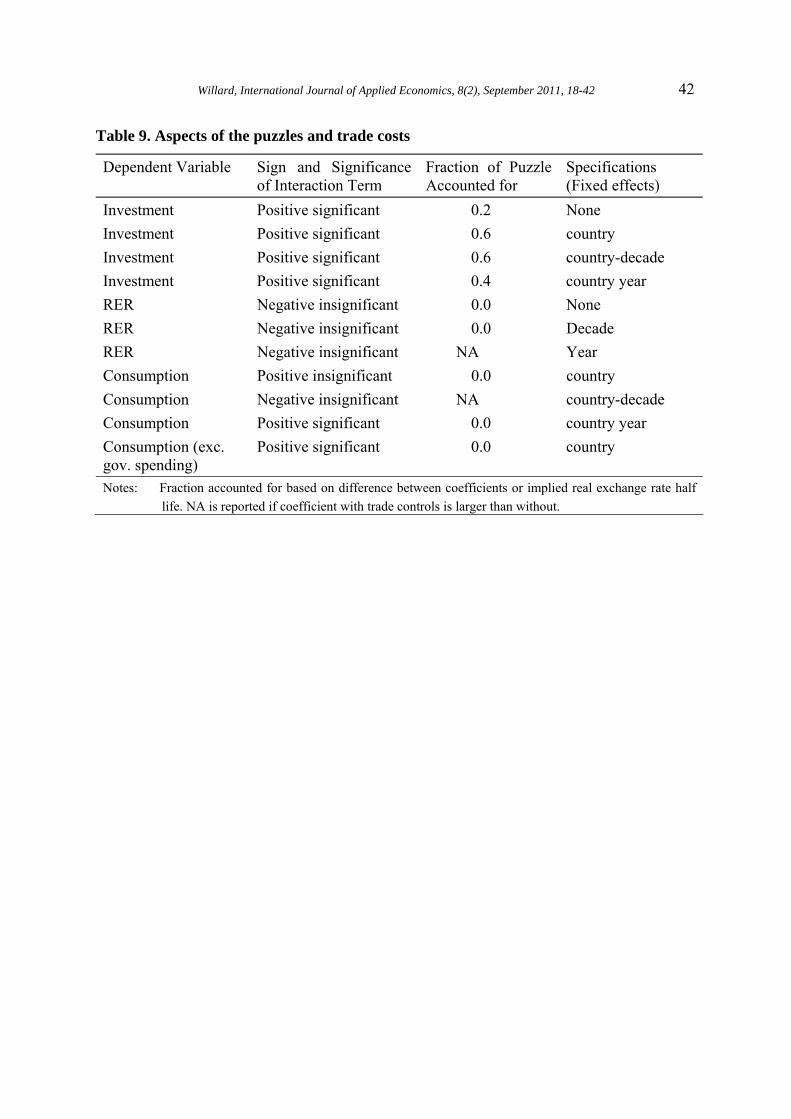
Table 9 provides information for addressing whether there are only certain aspects of the correlations that trade costs explain by summarizing results for different controls. It indicates that while trade costs play a role in some specifications, they play a minimal role in others. For example, the amount of the Feldstein-Horioka puzzle explained depends significantly on the controls. These results suggest that a well-defined notion of what aspects of the correlations are puzzling is needed before the role of trade costs have in the puzzles can be fully assessed.


7. Summary and Conclusions

Using panel data for a set of developed economies, this paper summarizes the correlation between trade costs and three important puzzles in international macroeconomics. It provides some evidence that the Feldstein-Horioka saving-investment puzzle is partially explained by trade costs. The signs of coefficient estimates imply that higher trade costs are associated with a stronger relationship between investment and saving. The size of the coefficients implies that these effects are economically important. Trade costs appear to explain little of the PPP or consumption correlation puzzles.

It is important to recognize that at best trade costs appear to explain certain aspects of the puzzles or correlations. Moreover as there is evidence that trade costs do not play a significant role in the PPP or consumption correlation puzzles, more work needs to be done to understand how trade costs relate to these puzzles. One plausible view is that all three puzzles should be linked because they are in some sense connected to issues of financial market imperfections. Potentially the developing theoretical literature on trade costs and some of the other puzzles in international macroeconomics (such as Coeurdacier, 2008) may provide more insights into the nature of the relationship and how to effectively examine it empirically. The empirical regularities presented in this paper should as a useful basis for assessing aspects of international macroeconomic theory.

Endnotes

* This project began while I was a doctoral student at Princeton University and an earlier version of the paper was completed at the Reserve Bank of Australia. Harald Anderson from the International Monetary Fund generously provided data on capital restrictions. I appreciate comments and suggestions by Alan Blinder, Russell Hillberry, David Hummels, Jarkko Jääskelä, Christopher Kent, Marion Kohler, Glenn Otto and Esteban Rossi-Hansberg as well as seminar participants at the Australasian Macroeconomics Workshop and the Reserve Bank of Australia, while conceding that any errors are my own. The paper does not necessarily reflect the views of the Reserve Bank of Australia or the Australian Government Treasury. Corresponding address: [email protected].

1. This puzzle was originally described by Feldstein and Horioka (1980). 2. Taylor (2000) discusses how without very specific data and consideration of the

institutional aspects of the market it is difficult to test for deviations from purchasing power parity.

3. For example in a world with two countries and identical constant relative risk aversion the share of consumption for each country is constant through time. In such a world, the


country’s share of world output should not explain the country’s share of world consumption in a particular year (see Obstfeld and Rogoff, 1996 Ch. 6). If it does, this suggests that more consumption smoothing is feasible. This is a justification for the regressions run here.

4. Some of the controls used later in the panel data regressions could be viewed as attempts to control for other possible explanations of the puzzles. This is particularly relevant for the Feldstein-Horioka puzzle for which a number of explanations already exist (though Obstfeld and Rogoff, 2001, describe them as not thoroughly convincing).

5. Obstfeld and Rogoff (Ch. 3, 1996) provide additional reasons to be sceptical. However, the regression results below with, for example, decade fixed effects may to some extent control for these other potential explanations of the puzzle, like demographic change.

6. An alternative approach could be to include trade cost terms in some of the popular nonlinear models such as ESTAR (see for example Kilian and Taylor, 2001).

7. The specification of Equation (3) has been driven by a desire to use a similar regression to that in Equations (1) to (2) while being similar to previous statistical examinations of the extent of complete insurance (for example Ch.5 of Obstfeld and Rogoff, 1996, Sørensen et al, 2005, and Townsend, 1994).

8. One potential concern with estimating Equation (3) is that it ignores the possibility that the consumption puzzle is explained by nontradeables consumption of goods like housing. There is some evidence that nontradeables can explain the consumption correlation puzzle (Lewis, 1996). Partly due to data availability and partly to examine how much of the puzzle can be explained by trade costs alone, the analysis does not take into account the role of nontradeables.

9. A series of papers by Papell and co-authors raise a number of concerns about existing studies into the persistence of real exchange rates. Some of the results provide evidence that the real exchange rate may have a unit root (e.g. Lopez, Murray and Papell, 2005, and Murray and Papell, 2005). While the papers of Papell suggest that estimating Equation (2) above may lead to an understating of the PPP puzzle, the similar estimates in rows 1 and 11 (which has more lags of the first difference in the real exchange rate) in Table 3 could be interpreted as suggesting it is not a major issue, though the differently signed coefficients (even if they are statistically insignificant) make this harder to defend.

10. Unlike Taylor (1994) relative prices are not included as controls as they may be related to the relative prices faced by locals and foreigners.

11. The results are estimated using the mean group estimator used by Imbs et al. (2005) and discussed in Pesaran and Smith (2005) and allows country fixed effects.

12. The results reported here use exchange rate measures of consumption and output, which could be viewed as more relevant if financial flows are the smoothing mechanism. In earlier analysis similar results were obtained using PPP based measures of consumption and output (results available on request).


References

Asdrubali, P., Sørensen, B.E. and O. Yosha. 1996. “Channels of Interstate Risk Sharing: United States 1963-1990,” Quarterly Journal of Economics 111(4), 1081-1110.

Baxter, M. and M.J. Crucini. 1993. “Explaining Saving-Investment Correlations,” American Economic Review 83, 416-436.

Coeurdacier, N. 2008. “Do Trade Costs in Goods Market Lead To Home Bias in Equities?” Centre for Economic Policy Research Discussion paper No. 6991.

Dumas, B. 1992. “Dynamic Equilibrium and the Real Exchange Rate in a Spatially Separated World,” Review of Financial Studies 5(2), 153–180.

Engel, C. 2000. “Comments on Obstfeld and Rogoff’s “The Six Major Puzzles in International Macroeconomics: Is there a Common Cause?”” NBER working paper no 7818.

Fazio, G., MacDonald, R. and J. Melitz. 2005. “Trade Costs, Trade Balances and Current Accounts: An Application of Gravity to Multilateral Trade,” CESifo working paper no 1529.

Feenstra, R. 2005. U.S. Import Data available at http://cid.econ.ucdavis.edu/data/sasstata/usiss.html

Feldstein, M. and C. Horioka. 1980. “Domestic Saving and International Capital Flows,” Economic Journal 90, 314–329.

Froot, K.A. and K. Rogoff. 1995. “Perspectives on PPP and Long-Run Real Exchange Rates” Grossman, G., and K. Rogoff (Eds.) Handbook of International Economics, vol. 3.

Ghironi, F. and M.J. Melitz. 2005. “International Trade and Macroeconomic Dynamics with Heterogeneous Firms,” Quarterly Journal of Economics 120(3), 865-915.

Hummels, D. 1999. “Have International Transportation Costs Declined?” mimeo University of Chicago. (http://www.mgmt.purdue.edu/faculty/hummelsd/research/decline/declined.pdf)

Hummels, D. and V. Lugovskyy. 2006. “Are Matched Partner Trade Statistics a Usable Measure of Transportation Costs?” Review of International Economics 14(1), 69–86.

Imbs, J., Mumtaz, H., Ravin, M.O. and H. Rey. 2005. “Aggregation Bias DOES Explain the PPP Puzzle,” NBER working paper no 11607.

Kehoe, P.J. and F. Perri. 2002. “International Business Cycles with Endogenous Incomplete Markets,” Econometrica 70(3), 907–928.

Kilian, L. and M.P. Taylor. 2001. “Why is it so Difficult to Beat the Random Walk Forecast of Exchange Rates?” European Central Bank working paper no 88.

Lewis, K.K. 1996. “What Can Explain the Apparent Lack of International Consumption Risk Sharing?” Journal of Political Economy 104(2), 267–297.

http://cid.econ.ucdavis.edu/data/sasstata/usiss.html

http://www.mgmt.purdue.edu/faculty/hummelsd/research/decline/declined.pdf


Lopez, C., Murray, J.C. and D.H. Papell. 2005. “State of the Art Unit Root Tests and Purchasing Power Parity,” Journal of Money, Credit and Banking 37(2), 361-369.

Murray, J.C. and D.H. Papell. 2005. “The Purchasing Power Parity Puzzle is Worse Than You Think,” Empirical Economics 30(3), 783-790.

Obstfeld, M. and K. Rogoff. 1996. Foundations of International Macroeconomics. Cambridge: MIT Press.

Obstfeld, M. and K. Rogoff. 2001. “The Six Major Puzzles in International Macroeconomics: Is there a Common Cause?” NBER Macroeconomics Annual 2000, 339–389.

Pesaran, M.H. and R. Smith. 1995. “Estimating Long-run Relationships from Dynamic Heterogeneous Panels,” Journal of Econometrics 68, 79–113.

Schnatz, B. 2006. “Is Reversion to PPP in Euro Exchange Rates Non-Linear?” European Central Bank working paper no 682.

Sørensen, B.E., Wu, Y., Yosha, O. and Y. Zhu. 2007. “Home Bias and International Risk Sharing: Twin Puzzles Separated at Birth,” Journal of International Money and Finance 26, 587-605.

Taylor, A.M. 1994. “Domestic Saving and International Capital Flows Reconsidered,” NBER working paper no 4892.

Taylor, A.M. 2000. “Potential Pitfalls for the Purchasing-Power-Parity Puzzle? Sampling and Specification Biases in Mean-Reversion Tests of the Law of One Price,” NBER working paper no 7577.

Townsend, R.M. 1994. “Risk and Insurance in Village India,” Econometrica 62(3), 539–591.

van Wincoop, E. and F.E. Warnock. 2010. “Can trade costs in goods explain home bias in assets?” Journal of International Money and Finance 29, 1108-1123.


Table 1. Summary Statistics

1974–1986 1987–1996 1997–2006

Trade costs (CIF compared to FAS) (%) Average (Standard deviation) 7 (3) 5 (2) 4 (2) Maximum 16 12 13 Minimum 1 1 0 Trade costs (also including duties) (%) Average (Standard deviation) 11 (5) 8 (3) 5 (3) Maximum 57 16 15 Minimum 2 2 1 Other variables Real exchange rate average (St. dev.) 94 (15) 98 (13) 96 (7) Investment (% of GDP) average (St. dev.) 25 (4) 22 (4) 22 (3) Saving (% of GDP) average (St. dev.) 23 (5) 23 (5) 24 (6) Ln(output/output world) average (St. dev.) 1.3 (0.3) 1.4 (0.3) 1.4 (0.3) Ln(cons/cons world) average (St. dev.) 1.3 (0.3) 1.4 (0.3) 1.4 (0.3) Capital controls average 0.7 0.5 0.1 Investment and saving correlation 0.54 0.52 0.09 Real exchange rate and one year lag correl. 0.83 0.90 0.86 Consumption and output regression coef. 0.81 0.75 0.72 Notes: These are summary statistics where each observation is country-year and all trade cost numbers are

rounded to whole numbers. There are 273 observations on trade costs for 1974–1986, 210 for 1987–1996 and 210 for 1997–2006. For the same decades the number of observations used for calculating the Investment and real exchange rate correlations are 273 and 222 for 1974–1986, 210 and 210 for 1987–1996 and 210 and 210 for 1997–2006. The last row reports results controlling for country fixed effects. In subsequent analysis the 3 periods above are treated as “decades” for the decade fixed effects.


Table 2. Investment (Equation 1) Model with country fixed effects

Trade cost measure

Specification Saving Trade cost Interaction term

1 With duties Baseline specification 0.14* (0.07)

-0.47* (0.15)

0.04* (0.01)

2 Without trade costs

Baseline specification 0.34* (0.06)

NA NA

3 With duties With country-decade fixed effects

0.27* (0.10)

-0.66* (0.15)

0.04* (0.01)


With country-decade fixed effects

0.67* (0.06)

NA NA

5 No duties Baseline specification 0.12 (0.07)

-0.66* (0.21)

0.06* (0.01)

6 With duties With additional control(a) 1.17 (1.16)

-0.50* (0.16)

0.04* (0.01)

7 With duties Robust regression(b) 0.37* (0.04)

-0.24* (0.10)

0.03* (0.004)

8 No duties Trade cost average of whole sample

0.02 (0.07)

NA 0.10* (0.01)

9 With duties Trade cost average of whole sample

-0.05 (0.08)

NA 0.08* (0.01)

10 With duties IV (lagged costs as instruments)(c)

0.36 (0.23)

0.37 (0.87)

0.01 (0.03)

11 With duties Alternative Investment Measure 0.16* (0.08)

-0.13 (0.19)

0.02* (0.01)

12 With duties With productivity and demographic controls

0.03 (0.07)

-0.56* (0.16)

0.04* (0.01)

Notes Robust standard errors are reported in parentheses. There are 693 observations used to estimate the results in the first row and the R-squared of the regression is 0.57.* indicates significance at the 5 per cent level. NA indicates no available estimate either because the terms are not included in the regression or because the variable is co-linear with the fixed effects. (a) Additional control is log distance interacted with the main independent variable (here saving). (b) Calculated using Stata’s rreg command. (c) Based on Stock-Yogo critical values the instruments are not weak.


Table 3. Real Exchange Rate (Equation 2) Model with no fixed effects

Trade cost measure

Specification Lagged real exchange rate

Trade cost

Interaction term

1 With duties Baseline specification 0.84*

(0.04) 0.01 (0.02)

-0.002 (0.001)



NA NA

3 With duties

Decade fixed effects 0.84* (0.04)

0.005 (0.02)

-0.001 (0.005)


Decade fixed effects 0.67* (0.06)

NA NA

5 No duties Baseline specification 0.81* (0.05)

-0.02 (0.03)

0.003 (0.01)

6 With duties With additional control(a) -3.30

(2.71) 0.01 (0.02)

-0.002 (0.004)

7 With duties Robust regression(a) 0.88*

(0.03) -0.01 (0.01)

0.002 (0.003)


0.76* (0.11)

-0.08 (0.09)

0.02 (0.02)

9 With duties

Trade cost average of whole sample

0.70* (0.14)

-0.10 (0.08)

0.02 (0.02)

10 With duties

IV (lagged costs as instruments)(b)

1.33* (0.18)

0.23 (0.09)

-0.05* (0.02)

11 With duties

With four lags of first difference of lagged RER

0.91* (0.04)

-0.03 (0.02)

0.006 (0.004)

12 With duties

Estimated in first differences using IV (country fixed effects)

0.86* (0.06)

0.06 (0.05)

-0.02 (0.01)

13 With duties

Using Mean Group Estimator/Imbs et al. monthly data (Using Imbs’ data)

0.97 -0.005 0.0008

Notes: Robust standard errors are reported in parentheses. There are 642 observations used to estimate the results in the first row and the R-squared of the regressionis 0.75.* indicates significance at the 5 per cent level. NA indicates no available estimate either because the terms are not included in the regression or because the variable is co-linear with the fixed effects. (a) see Table 2. (b) Based on Stock-Yogo critical values the instruments are not weak.


Table 4. Consumption (Equation 3) (inc. government spending) – country fixed effects

Trade cost measure

Specification Output Trade cost Interaction term


-0.003 (0.004)

0.003 (0.002)



NA NA


-0.015* (0.004)

0.010* (0.003)

4 With duties Consumption inc statistical discrepancy

0.70* (0.03)

-0.006* (0.003)

0.005* (0.002)

6 With duties With Additional control(a) -3.52* (0.70)

-0.004 (0.003)

0.003 (0.002)

7 With duties Robust regression(a) 0.71* (0.02)

-0.018* (0.001)

0.012* (0.001)


0.51* (0.02)

NA 0.064* (0.007)

9 With duties Trade cost average of whole sample

0.47* (0.02)

NA 0.050* (0.005)

10 With duties IV (lagged costs as instrument)(b)

0.65* (0.08)

-0.007 (0.007)

0.005 (0.004)

11 With duties Estimated in first differences 0.66* (0.03)

0.001 (0.001)

-0.001 (0.001)

12 With duties Year dummies 0.61* (0.03)

-0.005* (0.002)

0.007* (0.002)

13 With duties Consumption (exc. government spending)

0.68* (0.03)

-0.001 (0.002)

0.003 (0.002)

14 With duties Including demographic controls

0.59* (0.03)

-0.003* (0.001)

0.006* (0.001)

Notes: Robust standard errors are reported in parentheses. There are 692 observations used to estimate the results in the first row and the regression has a R-squared of 0.99. * indicates significance at the 5 per cent level. NA indicates no available estimate either because the terms are not included in the regression or because the variable is co-linear with the fixed effects. (a) see Table 2. (b) Based on Stock-Yogo critical values the instruments are not weak.


Table 5. Consumption (Equation 3) (inc. government spending) – decade-country fixed effects

Trade cost measure

Specification Output Trade cost Interaction term


0.002 (0.002)

-0.002 (0.002)



NA NA


-0.001 (0.006)

-0.0003 (0.004)

4 With duties Consumption inc. statistical discrepancy

0.79* (0.03)

-0.0009 (0.002)

0.001 (0.002)

Notes: Robust standard errors are reported in parentheses. * indicates significance at the 5 per cent level. There are 692 observations used to estimate the results in the first row. NA indicates no available estimate either because the terms are not included in the regression or because the variable is co-linear with the fixed effects.


Table 6. Trade costs, capital controls and the puzzles Dependent variable, fixed effects

Main independent variable (saving, exchange rate or output)

Interaction of capital control, trade cost and main independent variable

Interaction of trade cost and main independent variable

Investment country effects

0.20* (0.08)

-0.01 (0.01)

0.02* (0.01)

Investment country-decade effects

0.30* (0.12)

0.007 (0.02)

0.04* (0.01)

Investment country and year effects

0.10 (0.07)

-0.02 (0.01)

0.02* (0.01)

RER no fixed effects

0.76* (0.08)

-0.02 (0.01)

0.006 (0.01)

RER decade effects

0.76* (0.08)

-0.02* (0.01)

0.006 (0.01)

RER year effects

0.79* (0.08)

-0.01 (0.01)

0.002 (0.01)

Consumption country effects (inc. gov. spending)

0.72* (0.04)

0.003 (0.004)

-0.005 (0.003)

Consumption country effects (exc. gov. spending)

0.73* (0.03)

0.003 (0.004)

-0.003 (0.003)

Notes: Robust standard errors are reported in parentheses. * indicates significance at the 5 per cent level. 652 observations are used to estimate the investment equations, 604 the exchange rate equations and 651 the consumption equations.


Table 7. Trade costs and the puzzles (2nd approach, including duties)

Model Main independent variable (saving, exchange rate or output)

Interaction term

Fixed effects

Investment -0.03 0.03 Country Investment 0.46 0.02 Decade-

country RER 0.87 -0.003 None RER 0.87 -0.003 Decade Consumption (inc. gov. spending)

0.73 -0.003 Country

Consumption (inc. statistical discrepancy)

0.73 0.0004 Country

Table 8. Openness and the puzzles

Trade cost measure

Model Main independent variable (saving, exchange rate or output)

Interaction term Fixed effects

With duties

Investment 0.63* (0.08)

-0.001 (0.001)

Country

With duties

Investment 0.72* (0.012)

-0.001 (0.002)

Country-decade

With duties

RER 0.88* (0.05)

-0.001 (0.001)

None

With duties

RER 0.87* (0.05)

-0.0009 (0.0009)

Decade

With duties

Consumption (inc. gov. spending)

0.91* (0.03)

-0.003* (0.0003)

Country

With duties

Consumption (exc. gov. spending)

0.97* (0.02)

-0.003* (0.0002)

Country

Notes: Robust standard error reported in parentheses. * indicates significance at the 5 per cent level. Openness measure is openness (exports plus imports all over GDP) in constant prices from Penn World Tables.


Table 9. Aspects of the puzzles and trade costs

Dependent Variable Sign and Significance of Interaction Term

Fraction of Puzzle Accounted for

Specifications (Fixed effects)

Investment Positive significant 0.2 None Investment Positive significant 0.6 country Investment Positive significant 0.6 country-decade Investment Positive significant 0.4 country year RER Negative insignificant 0.0 None RER Negative insignificant 0.0 Decade RER Negative insignificant NA Year Consumption Positive insignificant 0.0 country Consumption Negative insignificant NA country-decade Consumption Positive significant 0.0 country year Consumption (exc. gov. spending)

Positive significant 0.0 country

Notes: Fraction accounted for based on difference between coefficients or implied real exchange rate half life. NA is reported if coefficient with trade controls is larger than without.

Documents

Trade Costs and Puzzles in International … International Journal of Applied Economics, 8(2), September 2011, 18-42 18 Trade Costs and Puzzles in International Macroeconomics Luke