Trade, capital accumulation and structural unemployment: anempirical study of the Singapore economy∗

Hiau Looi Keea,†, Hian Teck HoonbaDevelopment Economics Research Group, The World Bank,1818 H Street N.W., Washington, DC 20433, USA

bSchool of Economics and Social Sciences, Singapore Management University, 469 Bukit Timah Road, Singapore 259756

Abstract

This paper studies the factors responsible for the secular decline of Singapore’s unemploymentrate over the period 1966-2000 in an environment of low and stable inflation rates. We introducewage bargaining and unions into a specific-factors, two-sector economy with an export sector and anon-tradable sector to obtain an endogenous natural unemployment rate. Increases in the relativeexport price and capital stock in the export sector are predicted to reduce structural unemploy-ment. These hypotheses could not be rejected based on structural estimations and co-integrationregressions. Empirically, capital accumulation in the export sector explains most of the decline inSingapore’s unemployment rate.Keywords: endogenous natural rate of unemployment, wage bargaining, specific-factors model,

Stolper-Samuelson effect, Rybczynski effect.JEL Classification: E24, F12, J51

∗The authors thank two anonymous referees for their detailed comments on an earlier draft of this paper. The authorsare also grateful to Marcelo Olarreaga, seminar participants at the University of California at Davis and the World Bank.

†Corresponding author. Tel.: +1-202-473-4155; fax: +1-202-522-1159. E-mail addresses: hlkee@worldbank.org (H.L.Kee), hthoon@smu.edu.sg (H.T. Hoon).

1

Pub

lic D

iscl

osur

e A

utho

rized

Pub

lic D

iscl

osur

e A

utho

rized

Pub

lic D

iscl

osur

e A

utho

rized

Pub

lic D

iscl

osur

e A

utho

rized

Pub

lic D

iscl

osur

e A

utho

rized

Pub

lic D

iscl

osur

e A

utho

rized

Pub

lic D

iscl

osur

e A

utho

rized

Pub

lic D

iscl

osur

e A

utho

rized

Nontechnical Summary

The past three and a half decades witnessed a distinctly declining trend in Singapore’s unemploy-

ment rate, which dropped from an average annual rate of 7.85% in 1966-70 to 2.74% in 1991-2000.

This paper seeks to identify and empirically examine the factors that have influenced Singapore’s

unemployment rate in an environment of low and stable inflation. We incorporate a union bargaining

framework into a standard specific factor trade model, in which an increase in the relative price or

capital stock in the export sector raises the demand wage that firms can afford to pay relative to

workers’ fall-back income, and consequently lowers equilibrium unemployment. The magnitude of the

effects depends on the fall-back income, the weight unions attach to employment and the elasticity of

labor demand. The empirical section of the paper focuses on estimating these parameters using data

on Singapore. The results show that labor unions in Singapore care more about employment than

wages. Together with a small fall-back income and elastic labor demand, we show that given the same

percentage change in relative export prices and capital accumulation in the export sector, the effect

on unemployment is larger for the former. However, the empirical importance of capital accumulation

in the export sector dominates increases in relative export prices in reducing unemployment since

the manufacturing sector experienced a tremendous increase in capital inputs throughout the sample

period, whereas the relative price of exports experienced a far smaller increase and only in the early

part of the sample period. We conclude that through a very open trading regime, the tremendous

increase in capital stock of the exporting sector has been the main reason behind Singapore’s declining

unemployment rate.

2

1 Introduction

Prior to the seminal papers by Friedman (1968) and Phelps (1968), which introduced the expectations-

augmented Phillips curve and the concept of the natural rate of unemployment, it was commonly held

that a policy maker could use fiscal and monetary stimulus to keep the economy at a permanently low

rate of unemployment as long as it was willing to tolerate a high enough rate of inflation. Friedman

and Phelps, however, argued that the actual unemployment rate could remain below a certain natural

rate only insofar as the monetary authority could generate an actual inflation rate that exceeded the

expected rate of inflation. Absent expectation errors, the economy would settle down at the natural

rate of unemployment.

That natural or equilibrium structural rate of unemployment was argued to be invariant to mon-

etary changes though not necessarily to real factors. However, there was little understanding about

how exactly real factors affected the natural rate. Things changed when several economists, including

Phelps himself, were spurred by the phenomenon of a persistent rise of unemployment in Western

Europe without unexpected disinflation to begin research into the set of factors determining the nat-

ural rate. The non-inflationary structural boom in the US as well as in a number of other OECD

economies in the late ’90s gave further impetus to this research. The result of the research is a set

of complementary theories that pinpoint the determinants of the equilibrium structural rate of unem-

ployment: the union bargaining model (McDonald and Solow, 1981 and Layard, Nickell and Jackman,

1991), the efficiency wage model (Shapiro and Stiglitz, 1984), the insider-outsider model (Lindbeck and

Snower, 1989), the search and matching model (Pissarides, 2000), intertemporal-equilibrium models

(Phelps, 1994), and the social programs and wage instability model (Ljungqvist and Sargent, 1998).1

Factors that have been highlighted as being relevant in determining the natural rate in these models

include demographic factors, social and unemployment insurance programs, minimum wage policies,

tax structure, productivity growth, and capital accumulation. In addition, theoretical pieces by David-

son, Martin and Matusz (1988, 1999), Matusz (1985, 1998), and Hoon (2000, 2001) also incorporated

equilibrium unemployment into general equilibrium trade models to show that the path of equilibrium

unemployment rate can be shifted by various forces acting on economies that are interlinked via the

international trading system.

On the empirical front, although Staiger, Stock and Watson (1997) points out that estimates of

1See Phelps and Zoega (1998) and Salemi (1999) for a review of the literature.

3

the natural rate of unemployment tend to be imprecise, there have been several recent studies that

attempt to estimate the natural rate of unemployment as well as test the natural rate hypothesis.

Gordon (1997) estimates a time path of the natural rate for the US from 1955:2-1996:2, and concludes

that the natural rate declined in the ’90s. Using a technique that embedded the Kalman filter within

the full-information maximum likelihood procedure, Salemi (1999) finds substantial post-war variation

in the US natural rate, although actual unemployment can deviate from the natural rate through price

surprises. While Gordon estimated a time-varying natural rate by assuming that the natural rate

takes a random walk, Salemi shows that a model where the natural rate responds to economic forces

outperforms the random walk model. Empirical results from both studies support the time-varying

natural rate hypothesis. Finally, studying the extraordinary structural boom of the late ’90s in the

US, Staiger, Stock and Watson (2002) concludes that the US natural rate had indeed declined.

Adopting an endogenous natural rate framework, this paper seeks to identify and empirically

examine the factors that have influenced Singapore’s unemployment rate, which came down from

nearly 9 percent in 1966 to less than 3 percent in the ’90s in an environment of low and stable inflation.

We are still left, however, with a choice of which theory of the labor market to use? Given the lack

of formal social programs and unemployment benefit system in Singapore, we could not adopt models

where such programs are crucial to the determination of equilibrium unemployment, such as that of

Ljungqvist and Sargent (1998).2 On the other hand, the strong influence of trade unions, organized

both at plant and industry levels, in determining labor market outcomes in Singapore suggests that

the adoption of the union bargaining model would bring us a step closer to reality.3 This explains our

modelling choice.

In particular, we adopt the McDonald-Solow union bargaining apparatus, which we apply to a

specific-factors trade model to study the determinants of the natural rate in a small open economy. The

equilibrium unemployment rate is determined at the intersection of a downward-sloping aggregate labor

demand curve and an upward-sloping wage curve, the latter being the outcome of a wage bargaining

process. Since there is a rent going to an employed worker, his welfare is unambiguously higher than

2It was only in October 2003 that a modest unemployment compensation scheme with an initial budget of S$40million was introduced in Singapore. The scheme, called the Work Assistance Programme, provides a monthly allowanceof S$400 for three months to unemployed individuals.

3See Singapore National Trades Union Congress (1987) for a chronology of trade union development in Singapore.Any dispute that arises in the process of negotiation between a trade union and management over collective agreementscan be referred to the Industrial Arbitration Court, which, since 1972, could make reference to the annual wage guidelinesissued by the National Wages Council in its deliberations.

4

that of an unemployed worker. We show that an increase in the capital stock in the export sector

raises the demand wage that firms can afford to pay relative to the worker’s fall-back income, and so

consequently lowers equilibrium unemployment. Also, with no unemployment benefits and the family

providing a kind of insurance in the form of food, transport and housing in the event a member loses a

job, the worker’s fall-back income can be thought of as indexed to the non-traded good.4 Consequently,

a rise in the relative price of exports also raises the demand wage relative to the worker’s fall-back

income and so lowers the natural rate. In comparison to a traditional (Walrasian) full-employment

specific-factors model, an increase in the relative price of exports and an increase in the capital stock

bring about a smaller rise in the wage because in our model, aggregate employment also expands in

response to these shocks. In other words, by relaxing the assumption of full-employment, the model has

a smaller Stolper-Samuelson effect and Rybzynski effect than in traditional full-employment models.

The theoretical model is tested using annual data for Singapore, from 1966 to 2000. We first present

some reduced-form regressions which capture the co-integration relationships among the variables in

long-run equilibrium, á la Engle and Granger (1987). Results of the co-integration regressions provide

support for our hypotheses that an increase in the relative price of exports and capital accumulation

in the export sector decrease the long-run equilibrium unemployment rate. We then apply a three-

stage least squares regression to estimate the structural non-linear model, assuming that both relative

export prices and capital accumulation are exogenous. The estimation results once again provide

support for our hypotheses. We further instrument relative export prices and capital accumulation

with GMM estimation, correcting for heteroscedasticity and MA(1) autocorrelation of the error terms.

The results remain quantitatively and qualitatively robust. Based on the estimated parameters, we

show that given the same percentage change in relative export prices and capital accumulation in the

export sector, the effect on unemployment is larger for the former. However, the empirical importance

of capital accumulation in the export sector dominates increases in relative export prices in reducing

unemployment since the manufacturing sector experienced a tremendous increase in capital inputs

throughout the sample period, whereas the relative price of exports experienced a far smaller increase

and only in the early part of the sample period. These results are robust to omitted variable bias and

autoregressive heteroscedastic errors.

The rest of the paper is organized as follows: Section 2 presents some preliminary evidence that

4Close to 90 percent of Singaporeans live in public housing developed by the Housing Development Board.

5

the natural rate of unemployment in Singapore has declined over the past three and a half decades. In

Section 3, the theoretical model for estimation, namely the McDonald-Solow union bargaining model

with the specific-factors setup, will be presented. The empirical strategy of the paper is discussed in

Section 4, followed by data description in Section 5. We present the empirical results in Section 6,

and conclude the paper in Section 7.

2 Preliminary evidence of Singapore’s declining natural rate

The past three and a half decades witnessed a distinctly declining trend of Singapore’s unemployment

rate, which dropped from an average annual rate of 7.85% in 1966-70 to 2.74% in 1991-2000. Most

of the decline took place within the first two decades (see Table 1). Figure 1 shows the scatter

plot of the change in Singapore’s inflation rate from the last year to the current year against the

contemporaneous unemployment rate from 1966 to 2000. If a stable Phillips curve with a constant

natural rate exists, we ought to observe a negatively-sloped schedule. Instead, the plot depicts a near-

horizontal line, indicating that a steady decline of the unemployment rate has occurred in Singapore

without fuelling inflationary pressures. Such a relationship could be verified by a simple ordinary

least squares regression of the change in inflation rate on the contemporaneous unemployment rate,

as shown in Table 2. Since the estimated coefficient is not significantly different from zero, we cannot

statistically reject the hypothesis that a stable Phillips curve with a constant natural rate does not

exist.

A similar result is obtained for a sample of other fast-growing economies in the Asian region.

Figure 2 presents the same scatter plot for the other “miracle” economies, including Hong Kong (H),

South Korea (K) and Taiwan (T), as well as some neighboring countries, Indonesia (I), Malaysia (M)

and Thailand (L), controlling for country and year fixed effects, from 1980 to 2000. It is clear from the

plot that the slope of the regression line is very similar to the previous plot for Singapore, being flat

across countries and years in the sample.5 The preliminary evidence gives us encouragement to test

formally (in later sections) a theory of an endogenous natural rate based on Singapore data, and as

5The slope of the line is estimated by fitting the change in inflation rate on unemployment rate in the following panelregression:

ict = α0 + αc + αt + βuct + εct,

where subscript c and t denote country and year, respectively. White robust standard error is reported. Total numberof observations is 92, with R-square of 0.39. Data source: World Bank (2003).

6

we shall see, there is strong evidence that real forces, in particular, relative export prices and capital

accumulation in the export sector, strongly influence the natural rate of unemployment. The evidence

is suggestive that such a theory may also be applicable to some of the other Asian economies but a

formal test will have to await future research.

The following sections formally develop and test a model that captures the effects of international

trade and capital accumulation on the natural rate of unemployment of a small open economy.6

3 Theoretical model

In this section, we incorporate the McDonald-Solow union bargaining apparatus within a specific-

factors model. We assume that there are two sectors–X and Y–and two factors of production–

labor (L) and capital (K). X is assumed to be the export (manufacturing) sector and Y is the

non-tradable service sector. We assume that there are numerous firms in the two sectors of the

economy and that wage bargaining takes place with firm-level unions.7 (Although we model wage

bargaining explicitly, as McDonald and Solow (1981) note, the results of the union bargaining model

apply even where an informally organized labor pool bargains implicitly with one or more long-time

employers.) Nevertheless, workers are free to move between the two sectors. On the other hand,

capital is heterogeneous and sector specific. Hence it is not free to move between the manufacturing

and service sectors.8

Let’s assume that there are I identical firms in sector X, each with a production function (x)

presented in (1), and J identical firms in sector Y , each with a production function (y), as shown in

(2), I and J being large numbers. As characterized in (1) and (2), the technology is assumed to be

constant returns to scale, that is, homogeneous of degree one, with α being the capital elasticity in

the production of both sectors.9 The sectoral production of either good in the economy is simply the

product of the output of a typical firm, x or y, and the number of firms, I or J , respectively, in the

6Singapore’s total merchandise trade to GDP ratio stands at nearly 300 percent, reflecting the importance of re-processing of intermediate inputs for export.

7Given our simplifying assumption of a common elasticity of labor demand across sectors, our results below are robustto the alternative assumption of wage bargaining at the sectoral level.

8The immobility of capital between manufacturing and service sectors may not be as restrictive an assumption as itfirst appears since at least 80 percent of the capital investment in the manufacturing sector is foreign direct investmentfrom MNCs. It is not unreasonable to suppose that the MNCs stay within the manufacturing sector since the Singapore-based subsidiaries are just part of the global production networks of the MNCs.

9Alternatively, under the neoclassical assumptions of perfect competition and constant returns to scale, we caninterpret α as the aggregate (average) capital share of the economy.

7

sector.

Assume that each firm maximizes its own profits and that the goods markets are perfectly compet-

itive. Labor, while participating in firm-specific unions, is free to move between sectors, so the return

to labor in both sectors will be equalized in equilibrium. Capital, assumed to be non-homogeneous, is

the specific factor that does not move across sectors. The equilibrium return to factors will be equal

to the respective values of marginal product.

The equilibrium real wage rate, w, and rental rate, r, with good Y as the numeraire, are represented

by (3) and (4). Notice that in (4), the returns to capital in both sectors are not equal under the

assumption that capital is not a homogeneous factor that can easily move between sectors. On the

other hand, (3) shows that the real wage rate is equal in both sectors due to the assumption of perfect

labor mobility.

x = N1−αx Kα

x , X = x = Ix, (1)

y = N1−αy Kα

y , Y = y = Jy, (2)

w = p (1− α)KxNx

α

= (1− α)KyNy

α

, (3)

rX = pαKxNx

−(1−α)= rY = α

KyNy

−(1−α), (4)

p ≡ PXPY, w ≡ W

PY, rX ≡ RX

PY, rY ≡ RY

PY, (5)

N = NX +NY , NX = Nx = INx, NY = Ny = JNy, (6)

KX = Kx = IKx, KY = Ky = JKy, (7)

u ≡ 1− NL> 0. (8)

It is clear that the relationship between the relative price of goods and the capital-labor ratio is

crucial for understanding the other relationships. The higher the relative price of good X to good Y ,

the lower the capital-labor ratio in sector X as labor, the mobile factor, is attracted to sector X to

work with the given stock of capital. Eq. (5) gives us the identity of relative price of goods, p, and

the real factor returns, w, rX and rY with PX , PY , W , RX and RY denoting their respective nominal

values. Eq. (6) shows the sectoral distribution of total employment in the economy, with N being the

total employed labor force in both sectors. NX and NY are the sectoral employment levels, which are

the summation of the number of workers employed in each sector. Similarly, KX and KY denote the

8

sectoral capital stocks, which are the summation of the capital stocks of all the firms in each sector. As

shown in (8), and will be proven later, total labor force, L, in this non-Walrasian economy is greater

than the total employment, N . In other words, the equilibrium unemployment rate, or the natural

rate of unemployment, u ≡ 1− (N/L), is positive.Assume that within each sector there are identical firm-specific labor unions that only bargain

over the real wage of the members and let the respective firms decide on employment at any set

wage. The objective of each of these unions is to maximize the wage difference between members and

non-members, as represented in the Cobb-Douglas utility function of the union, subject to the labor

demand function of the firm. For a representative firm-specific union in sector X, the optimization

problem is:

max Ux = Nτx (wx −A)1−τ

s.t. wx = p (1− α)KxNx

α

,

A ≡ (1− u)w + uB.

Here, Nx is the number of workers employed in firm x for a given bargained wage according to the

labor demand function given in (3). Both Nx and wx enter the utility function of the union with the

weights of τ and 1− τ , respectively. A higher τ implies that the union cares more about employment

than the wage difference. As will be shown later, τ indeed is an important parameter that determines

the wage bargaining equilibrium, and hence the natural rate of unemployment.

The real wage, wx, is set by the union and A is the expected real income elsewhere should the

worker lose his job at the current firm. The variable A is the sum of two terms; the first term depends

on the wage that can be earned elsewhere in the economy, w , adjusted by the probability of getting

a job should a worker leave his or her current firm, which we proxy by the rate of employment, 1− u.(Of course, in the symmetric equilibrium we consider, with workers freely mobile across sectors, we

ultimately have wx = wy = w .) The second term in A is given by unemployed income B. In theory,

the unemployed income, B, could be taken as the unemployment benefit or non-wage income when

the worker is unemployed. In Singapore, however, there was no official unemployment benefit given

by the state until its introduction in October 2003. Nevertheless, a worker, while employed, and

his employer are required to make a contribution to the Central Provident Fund (CPF). The CPF

contributions are a kind of compulsory saving that can be withdrawn with interest after a specified

9

official retirement age.10 Although workers might face liquidity constraints and can only draw out the

money after retirement, not when he becomes unemployed, the CPF savings could serve as a kind

of strategic wealth á la Bernheim, et al. (1985) that encourages intra-family transfers when a family

member is unemployed. Moreover, it is arguable that there is some social obligation in an Asian family

to provide for the basic necessities of a family member if he or she is in financial difficulties. We can,

therefore, think of B as the family insurance support that a family member can draw upon in the

unfortunate event that he or she loses a job. When one of the family members is thrown out of job, it

is very likely that the family will act as a supporting unit that provides food, housing and transport

in kind. For this reason, we can think of B as indexed to the price of the non-traded good.

In partial equilibrium, the bargained wage will be set at the level where the union’s indifference

curve is tangent to the firm’s labor demand curve. At the point of tangency, the slope of the indifference

curve equals to the slope of the labor demand curve. It is clear that in equilibrium, the wage markup

of the union is affected by the labor demand elasticity, α−1, which is also the inverse of the elasticity

of capital in a Cobb-Douglas production function.11 The more elastic the labor demand function, i.e.

the lower α, and/or the higher the employment weight of the union’s utility function, i.e. a larger τ ,

the lower the wage markup, as shown in (9):

wx −Awx

= α1

τ− 1 , (9)

WSCx : wx =A

1− α 1τ − 1

. (10)

The equilibrium relationship between wx and Nx is defined on a firm-level wage-setting curve

(WSCx), as shown in (10), obtained by re-arranging (9). Notice that at the firm level, given the

constant elasticity of labor demand, which is a property of the Cobb-Douglas production function, the

wage-setting curve does not depend on employment. It only depends on the labor demand elasticity,

10Subject to a minimum sum requirement that has to be left in the CPF, members can withdraw their compulsorysavings after age 55.11Labor demand elasticity, ε, is defined as

ε ≡ ∂ lnN

∂ lnw= α−1,

according to (3). Given (1), the Cobb-Douglas production function, α is also the elasticity of capital input, i.e.

∂ ln x

∂ lnKx= α, where

0 < α < 1.

Thus, the derived labor demand function has an elasticity that is greater than one.

10

α−1, weight of employment in the union’s objective function, τ , and the worker’s alternative income,

A.

Finally, given that the objective function of every union in both sectors X and Y is the same

and each small union faces an identical labor demand function in its respective firm in the sectors,

the general equilibrium of this decentralized wage bargaining economy will be reached when all the

identical unions in each firm bargains with the firm and sets the same wage. Therefore, in the general

equilibrium, we have the relationship given in (11), which leads to the aggregate wage-setting curve

(WSC) of the economy:

w = wx = wy, (11)

WSC : w =B

1− α( 1τ−1)1−(NL )

. (12)

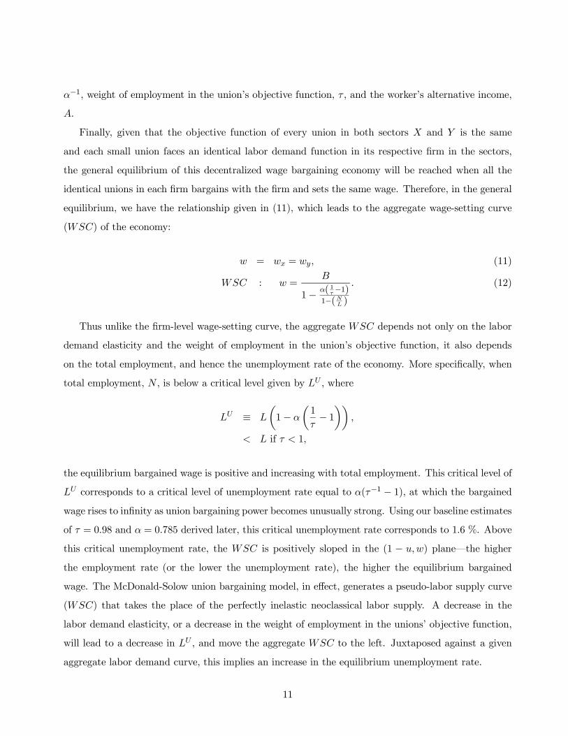
Thus unlike the firm-level wage-setting curve, the aggregate WSC depends not only on the labor

demand elasticity and the weight of employment in the union’s objective function, it also depends

on the total employment, and hence the unemployment rate of the economy. More specifically, when

total employment, N , is below a critical level given by LU , where

LU ≡ L 1− α1

τ− 1 ,

< L if τ < 1,

the equilibrium bargained wage is positive and increasing with total employment. This critical level of

LU corresponds to a critical level of unemployment rate equal to α(τ−1 − 1), at which the bargainedwage rises to infinity as union bargaining power becomes unusually strong. Using our baseline estimates

of τ = 0.98 and α = 0.785 derived later, this critical unemployment rate corresponds to 1.6 %. Above

this critical unemployment rate, the WSC is positively sloped in the (1 − u,w) plane–the higherthe employment rate (or the lower the unemployment rate), the higher the equilibrium bargained

wage. The McDonald-Solow union bargaining model, in effect, generates a pseudo-labor supply curve

(WSC) that takes the place of the perfectly inelastic neoclassical labor supply. A decrease in the

labor demand elasticity, or a decrease in the weight of employment in the unions’ objective function,

will lead to a decrease in LU , and move the aggregate WSC to the left. Juxtaposed against a given

aggregate labor demand curve, this implies an increase in the equilibrium unemployment rate.

11

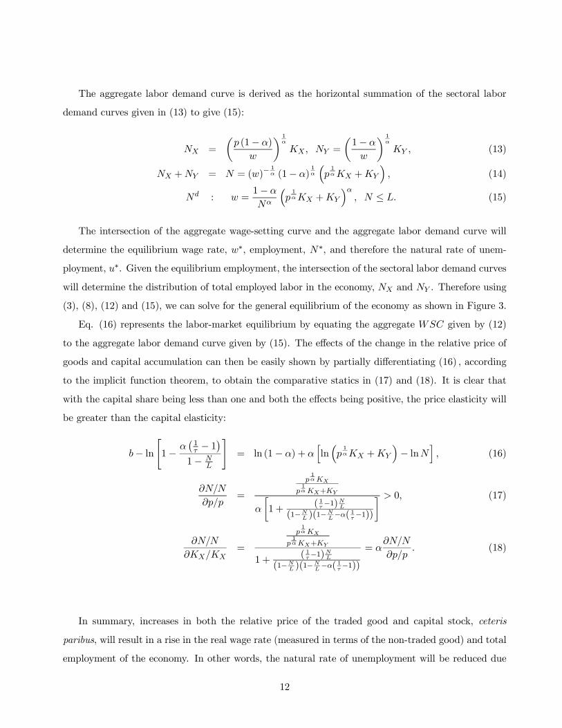
The aggregate labor demand curve is derived as the horizontal summation of the sectoral labor

demand curves given in (13) to give (15):

NX =p (1− α)

w

1α

KX , NY =1− α

w

1α

KY , (13)

NX +NY = N = (w)−1α (1− α)

1α p

1αKX +KY , (14)

Nd : w =1− α

Nαp1αKX +KY

α, N ≤ L. (15)

The intersection of the aggregate wage-setting curve and the aggregate labor demand curve will

determine the equilibrium wage rate, w∗, employment, N∗, and therefore the natural rate of unem-

ployment, u∗. Given the equilibrium employment, the intersection of the sectoral labor demand curves

will determine the distribution of total employed labor in the economy, NX and NY . Therefore using

(3), (8), (12) and (15), we can solve for the general equilibrium of the economy as shown in Figure 3.

Eq. (16) represents the labor-market equilibrium by equating the aggregate WSC given by (12)

to the aggregate labor demand curve given by (15). The effects of the change in the relative price of

goods and capital accumulation can then be easily shown by partially differentiating (16) , according

to the implicit function theorem, to obtain the comparative statics in (17) and (18). It is clear that

with the capital share being less than one and both the effects being positive, the price elasticity will

be greater than the capital elasticity:

b− ln 1− α 1τ − 11− N

L

= ln (1− α) + α ln p1αKX +KY − lnN , (16)

∂N/N

∂p/p=

p1αKX

p1αKX+KY

α 1 +( 1τ−1)NL

(1−NL )(1−N

L−α( 1τ−1))

> 0, (17)

∂N/N

∂KX/KX=

p1αKX

p1αKX+KY

1 +( 1τ−1)NL

(1−NL )(1−N

L−α( 1τ−1))

= α∂N/N

∂p/p. (18)

In summary, increases in both the relative price of the traded good and capital stock, ceteris

paribus, will result in a rise in the real wage rate (measured in terms of the non-traded good) and total

employment of the economy. In other words, the natural rate of unemployment will be reduced due

12

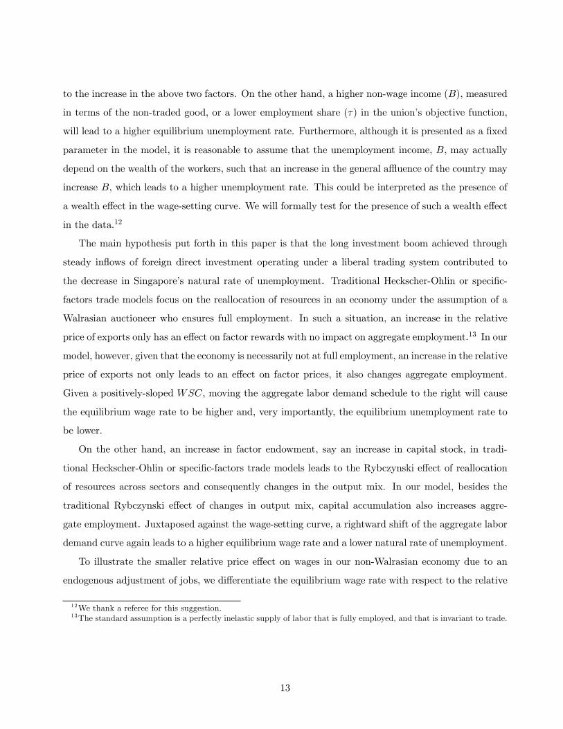
to the increase in the above two factors. On the other hand, a higher non-wage income (B), measured

in terms of the non-traded good, or a lower employment share (τ) in the union’s objective function,

will lead to a higher equilibrium unemployment rate. Furthermore, although it is presented as a fixed

parameter in the model, it is reasonable to assume that the unemployment income, B, may actually

depend on the wealth of the workers, such that an increase in the general affluence of the country may

increase B, which leads to a higher unemployment rate. This could be interpreted as the presence of

a wealth effect in the wage-setting curve. We will formally test for the presence of such a wealth effect

in the data.12

The main hypothesis put forth in this paper is that the long investment boom achieved through

steady inflows of foreign direct investment operating under a liberal trading system contributed to

the decrease in Singapore’s natural rate of unemployment. Traditional Heckscher-Ohlin or specific-

factors trade models focus on the reallocation of resources in an economy under the assumption of a

Walrasian auctioneer who ensures full employment. In such a situation, an increase in the relative

price of exports only has an effect on factor rewards with no impact on aggregate employment.13 In our

model, however, given that the economy is necessarily not at full employment, an increase in the relative

price of exports not only leads to an effect on factor prices, it also changes aggregate employment.

Given a positively-sloped WSC, moving the aggregate labor demand schedule to the right will cause

the equilibrium wage rate to be higher and, very importantly, the equilibrium unemployment rate to

be lower.

On the other hand, an increase in factor endowment, say an increase in capital stock, in tradi-

tional Heckscher-Ohlin or specific-factors trade models leads to the Rybczynski effect of reallocation

of resources across sectors and consequently changes in the output mix. In our model, besides the

traditional Rybczynski effect of changes in output mix, capital accumulation also increases aggre-

gate employment. Juxtaposed against the wage-setting curve, a rightward shift of the aggregate labor

demand curve again leads to a higher equilibrium wage rate and a lower natural rate of unemployment.

To illustrate the smaller relative price effect on wages in our non-Walrasian economy due to an

endogenous adjustment of jobs, we differentiate the equilibrium wage rate with respect to the relative

12We thank a referee for this suggestion.13The standard assumption is a perfectly inelastic supply of labor that is fully employed, and that is invariant to trade.

13

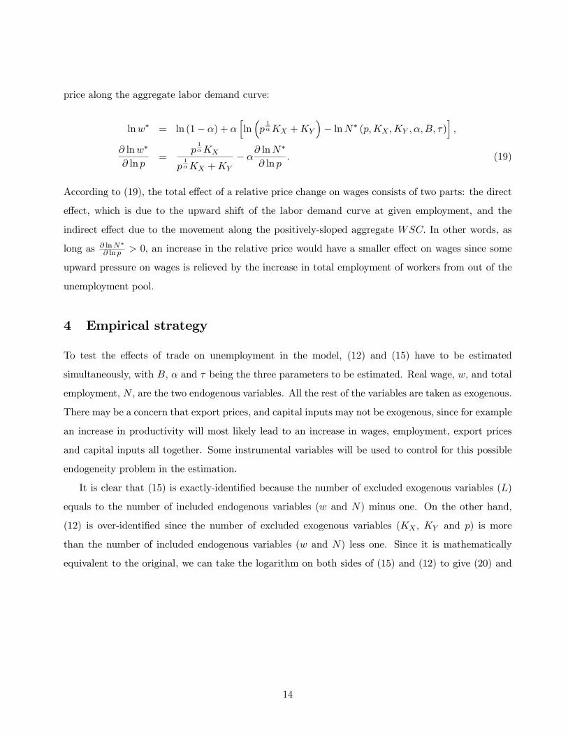
price along the aggregate labor demand curve:

lnw∗ = ln (1− α) + α ln p1αKX +KY − lnN∗ (p,KX ,KY ,α, B, τ) ,

∂ lnw∗

∂ lnp=

p1αKX

p1αKX +KY

− α∂ lnN∗

∂ ln p. (19)

According to (19), the total effect of a relative price change on wages consists of two parts: the direct

effect, which is due to the upward shift of the labor demand curve at given employment, and the

indirect effect due to the movement along the positively-sloped aggregate WSC. In other words, as

long as ∂ lnN∗∂ ln p > 0, an increase in the relative price would have a smaller effect on wages since some

upward pressure on wages is relieved by the increase in total employment of workers from out of the

unemployment pool.

4 Empirical strategy

To test the effects of trade on unemployment in the model, (12) and (15) have to be estimated

simultaneously, with B, α and τ being the three parameters to be estimated. Real wage, w, and total

employment, N , are the two endogenous variables. All the rest of the variables are taken as exogenous.

There may be a concern that export prices, and capital inputs may not be exogenous, since for example

an increase in productivity will most likely lead to an increase in wages, employment, export prices

and capital inputs all together. Some instrumental variables will be used to control for this possible

endogeneity problem in the estimation.

It is clear that (15) is exactly-identified because the number of excluded exogenous variables (L)

equals to the number of included endogenous variables (w and N) minus one. On the other hand,

(12) is over-identified since the number of excluded exogenous variables (KX , KY and p) is more

than the number of included endogenous variables (w and N) less one. Since it is mathematically

equivalent to the original, we can take the logarithm on both sides of (15) and (12) to give (20) and

14

(21) , respectively:

lnw = c+ ln (1− α) + α ln p1αKX +KY − lnN , (20)

lnw = b− ln 1− α 1τ − 11− N

L

, (21)

b ≡ lnB.

In (20), a constant term c is introduced with the similar purpose of any other constant term in normal

regressions, that is, to capture the effect of other important variables that are not included in the

model so that the residual will have a zero mean and therefore all the estimators will be unbiased.

Finally, given that the parameters in (20) and (21) are not linear to the dependent variables, we

first employ a non-linear three-stage least squares estimation with iterations, which is both consistent

and efficient if the exogenous variables are truly exogenous and the error terms are not autocorrelated

or heteroscedastic. To control for possible endogeneity, autocorrelation and heteroscedasticity, we also

fit the system of non-linear regressions using GMM estimation, which is both consistent and efficient.

5 Data description

The estimations were carried out using yearly data from 1966 to 2000, most of which are available in

the Report on the Census of Industrial Production and the Singapore Yearbook of Statistics. Besides

that, the Report on the Labor Force Survey and the Singapore Input-Output Tables 1988 also provided

some of the data. All nominal variables have been converted to real variables with 1990 as the base

year using appropriate price indices.

According to the Singapore Yearbook of Statistics, labor force data are based on the mid-year

Labor Force Surveys since 1974. For 1990, 1995 and 2000, labor force data were based on Population

Censuses and the mid-decade (1995) General Household Survey (GHS). Population Censuses and

the GHS collect data on the economic activities of the population, including detailed information on

employment and unemployment, characteristics of the labor force and economically inactive persons.

The data refer to persons aged 15 years or older. Unemployed persons refer to those who did not work

during the reference period but were available for work and were looking for a job with pay. Persons

in the process of starting their own business or taking up a new job after the reference period are also

considered as unemployed. Unemployment rate refers to unemployed persons as a percentage of the

15

total labor force, which includes both employed and unemployed persons during the reference period.

Given that Singapore follows the International Conference of Labor Statistics, such an unemployment

measure is standard and comparable to that of the US.

Wages of labor are defined as the total remuneration per worker. The coverage of total remuneration

includes the basic salary, employers’ and employees’ contributions to the Central Provident Fund,

bonuses, pensions paid by employers and other benefits provided. It is the total cost of hiring workers.

Real wage of workers is constructed by deflating the nominal wage by the price of non-traded goods.

To capture the effect of international trade on employment, according to the model, the price of

exports is needed to compute the value of the marginal productivity of worker in the export sector.

However, the published export price series is too short with the earliest available year being only 1974.

Thus it will decrease the degrees of freedom of our estimation. This problem has been solved after the

GDP deflator for the export of goods and services is used as a proxy for the export price index. It can

be checked that these two series of data are highly positively correlated, due to the fact that export

of services is relatively small compared to that of goods.14 As such, it is reasonable to use the GDP

deflator for export goods and services as a proxy for the price of exports.

An econometric concern regarding the use of Singapore’s data on the export price or the GDP

deflator for the export of goods and services is that it could be endogenous, and would lead to incon-

sistent and biased estimation of the parameters in the model. For example, higher productivity growth

of the export sector could lead to higher export prices and wages, which creates a spurious correlation

between the two variables. One way to tackle the endogeneity issue would be to use some instrumental

variable that is exogenous to domestic wages and yet highly correlated with export prices. Given that

most of the exports of Singapore are done by MNCs, the really relevant price that they face are the

exogenous world prices denominated in US dollars.15 Hence we use the price of export in constant

1990 US$ as instrument.

Similarly, the price of the non-traded good is needed to compute the value of marginal productiv-

ity of labor in the non-traded good sector. A series of the GDP deflator for the non-traded good is

generated by taking the weighted average of the GDP deflators of all the non-traded sectors in the

14After plotting the deflator together with the export price index, it is found that these two series of data almostoverlap with each other.15 In offering a wage to attract, say, a worker from the non-traded good sector to work in an MNC producing the export

good, the firm is interested in how much additional revenue the worker will generate in US$.

16

economy.16 The non-traded sector comprises Utilities, Construction, Commerce, Transport and Com-

munications, Financial and Business Services, and Other Services. The shares of the value of export

of these sectors in the total value of export of the economy, in Singapore Input-Output Tables 1988,

were 0.13 percent, 0 percent, 8.6 percent, 12.8 percent, 3.5 percent and 0.19 percent, respectively. In

the same time period, the export share of the manufacturing sector was about 75 percent.

Capital stock series of both sectors is computed from the respective gross real investment series,

using a perpetual inventory method and constant rates of depreciation. We estimate the initial capital

stock in 1960 using an infinite sum of investment, assuming the average growth rates of investment in

the first five years are good proxies for investment growth prior to 1960.17 Normally, gross investment

is defined as the difference between the expenditure and sale of capital goods in a given year. Due

to data constraint, the total domestic capital formation of the economy is taken as the total gross

investment of the whole economy, less the gross investment of the manufacturing sector, which is

generated in the normal way, giving us the gross investment in the non-traded good sector. The

nominal gross investment series in both sectors are then deflated by the GDP deflator of the domestic

capital formation to convert to the respective real gross investment series. The capital stock of the

non-traded sector is therefore defined as the total capital stock of the economy that is not accounted

for by the traded good sector.

In the absence of published depreciation rates by asset category, we adopt those used by Jorgenson

and Sullivan (1981). The respective depreciation rates for the four categories of capital input are

machinery and equipment (0.1047), office equipment (0.2729), transport (0.2935), and plants and

building (0.0361). Unless otherwise stated, the above data can be found in the Report on the Census

of Industrial Production, various years.

Table 1 presents the main data set with the sample mean and the average annual growth rate of each

16We use the respective shares of these sectors in GDP as the weights.17Specifically, let I1 be the first year the investment data is available, and let g be the average growth rate of investment

in the first five years. Let’s assume that there are infinite periods prior to period 1 where the investment is growing atthe same rate g but no data was collected. By assuming that the growth rate of investment of the first five years isrepresentative of the growth rate of investment prior to year 1, it can be shown that the initial capital stock is

K1 = I1

∞

l=0

1− δ

1 + g

l

=I1g + δ

.

17

variable. The annual average growth rate of real wage and employment are 4.4% and 4% respectively,

which indicate that both wages and employment have been growing throughout the sample period.

At the same time, the relative exports price index in US$ shows signs of a gradual increase up to the

late ’70s and remains relatively constant after that, while the growth rates of capital stock in both

sectors are more than 10% annually, with faster capital accumulation in the traded good sector. Thus,

even though both the relative price and the Rybczynski effects of trade are important theoretically,

the latter may have more relevance empirically. A series of selected variables is presented in Figure 4.

6 Empirical results

6.1 Reduced-form regressions

Before we present the estimation results of the structural model, some reduced-form regressions may

serve as base-line comparisons. Column (1) of Table 3 shows the log linear relationship between

the unemployment rate, the capital stock and the relative price of the tradable sector. It is clear

that increases in the capital stock and relative price of the tradable sector tend to reduce the overall

unemployment rate of Singapore. Both variables have statistically significant effects in decreasing

unemployment, and the movement of these two variables are sufficient for explaining 70 percent of the

movement of unemployment.

The next column controls for the capital stock of the non-tradable sector. An increase in the capital

stock of the non-tradable sector has two offsetting effects on the equilibrium unemployment rate.

First, according to the model, such an increase would raise the overall labor demand of the economy

by shifting the aggregate labor demand curve to the right and reduce the equilibrium unemployment

rate. Second, given that the level of alternative income of workers are likely to be indexed to the general

affluence of the country, which we can proxy by the increase in capital stock of the non-tradable sector

owned mainly by Singaporeans, an increase in the capital stock of the non-tradable sector would then

shift the wage-setting curve up and increase the unemployment rate.18 Empirically, the overall effect

of capital stock of the non-tradable sector on unemployment rate depends on the relative magnitude of

these offsetting effects. Results reported in column (2) show that the latter is greater than the former.

18According to data obtained from the Singapore Department of Statistics, the share of foreign equity in the non-tradable sector is around 17% on average, for the period 1970 to 1999. This indicates that a large majority of the assetsin the non-tradable sector is owned by Singaporeans, and makes it a reasonable proxy for the wealth of labor force, assuggested by the referee.

18

Thus, we find some empirical support for the wealth effect of capital accumulation in the non-tradable

sector, which increases the unemployment rate. However, controlling for capital stock of the non-

tradable sector does not affect the statistical relationships established in column (1), where the export

price increase and capital accumulation of the export sector are shown to reduce unemployment.

We further control for the change in the general CPI inflation rate in column (3). This is to

allow for the potential Phillips-curve type trade-off relationship between unemployment and price

innovation.19 If there is in fact such a relationship, we expect the estimated coefficient of the first

difference of inflation rates to be negative. The result presented in column (3) shows that while the

estimated coefficient is negative, it is not statistically different from zero. This is consistent with our

earlier result shown in Figure 1 and Table 2 that there is an absence of a stable Phillips curve with a

constant natural rate of unemployment in Singapore.

Column (4) controls for the log level of labor force in the reduced-form specification. An increase

in the labor force leads to a less than proportionate increase in the number employed, with the result

that the unemployment rate rises. Thus, we expect the estimated coefficient to be positive. The

reported estimated coefficient, however, is not statistically different from zero, which indicates that,

empirically, most of the movements in unemployment rate in Singapore are due to the movements in

relative prices and capital stocks, rather than labor force size. In other words, controlling for the size

of labor force does not change the estimated coefficients in column (2).

Finally, the regressions reported in Table 3 may be spurious in nature, given that all the series

may be non-stationary. While we control for autoregressive error terms by reporting the Newey-West

robust standard errors in the parentheses, it is however not sufficient to control for non-stationarity,

unless the series are co-integrated. In the event that the series are indeed co-integrated, while detrend-

ing or differencing the series would not be appropriate, the reduced-form regressions nonetheless are

consistent and have the nice interpretation of a long-run equilibrium relationship among the variables,

á la Engle and Granger (1987). Engle and Granger also propose a two-step procedure to estimate the

short-run dynamic fluctuations of the variables by an error-correction model.

To test for co-integration, we would first need to verify that the series are integrated of order

one, I (1) . Table 4 presents some unit root tests on the levels and first differences of the variables.

If the variables are I (1) , we would expect the levels to have unit roots and the first differences to

19We thank a referee for this suggestion.

19

be stationary. The unit root null hypothesis is rejected if the reported t-statistics is smaller than the

5% critical values. In the first row of Table 4, the level of unemployment rate is shown to follow a

random walk, while its first difference is stationary, since the respective t-statistics are -2.898 (>-2.975)

and -5.923(<-2.978). This indicates that unemployment rate is indeed I(1). Similarly, the log level

of relative export prices, employment, labor force and wages also follow random walks, while their

first differences are stationary, which signal that these series are also I (1) . On the other hand, both

the log levels of capital stock of the tradable and non-tradable sectors are shown to follow a random

walk with a sixth-order autoregressive error and have stationary first differences. This confirms that

both the levels of the capital stock series are I (1) .20 To establish that the series are co-integrated, we

also perform a unit root test on the regression errors of column (2) of Table 3, which is our preferred

reduced-form specification. The relevant t-statistics is -3.353 which is less than -1.95, the 5% critical

value as reported in Table 4. Thus we reject the spurious regression null hypothesis that the error has

unit root, in favor of a co-integration hypothesis. In other words, the unemployment rate, prices, and

the two capital stock series are co-integrated and the regression error is stationary. Thus the estimated

coefficients reported in column (2) form a consistent co-integration vector which represents a long-run

equilibrium relationship among the variables.

We completed the two-step procedure by fitting an error correction model based on the estimation

error terms from column (2) of Table 3. We report the results of regressing the change in unemployment

rate on its first lag, the error correction term, the first lagged changes in the tradable capital stock and

relative prices, and the second and fourth lagged changes in the non-tradable capital stock in Table

5. The error correction term is significant and has the right sign, which further indicates that the

co-integration regression in column (2) of Table 3 represents a long-run equilibrium relationship among

the variables. Figure 5 shows the fitted long-run and short-run unemployment rates, together with

the actual. It is clear that while the fitted long-run rate is declining, the fitted short-run year-to-year

unemployment rates fluctuate around the fitted long-run rate and track the actual unemployment rate

very well.21

20Notice that all of the series follow random walks and none of the series are trend stationary. This shows that it isnot appropriate to detrend the data, which could be counterproductive. For concreteness, we also include a time trendin the reduced-form regressions. As suspected, the estimated coefficient of time trend is not significant. This result isavailable upon request.21The correlation coefficients between the actual unemployment rate and the fitted long-run and short-run rates are

0.78 and 0.97, respectively.

20

6.2 Structural regressions

The estimation of the system of equations is first performed using non-linear three-stage least squares

with various iterative starting values of b, α, τ and c. Given that changing the starting values of the

parameters makes little difference to the estimation, we present one of the results of the estimation in

column (1) of Table 6 with the starting values of b, α, τ and c at 0, 0.01, 0.4, and 0 respectively.22

All the parameters are estimated with high statistical significance. The equations for the aggregate

wage-setting curve and the aggregate labor demand function are estimated with acceptable R-squares.

With the various starting values, after several rounds of iteration, the system converges to around the

point where the estimated values for b, α, τ and c are 8.98, 0.74, 0.98 and 7.71, respectively.

Column (2) deals with the possible endogeneity of our regressors by using the lagged values of

capital inputs in both traded and non-traded sectors, world price of exports, the total labor supply,

wages and unemployment rate as instruments for the GMM estimation.23 Given that the error terms

are very likely to be autocorrelated, we also incorporate a first-order moving-average, MA(1), process

in our estimation. The result of the GMM estimation is presented in column (2) of Table 6, where

heteroscedastic-consistent standard errors are reported. It is obvious that controlling for endogeneity,

autocorrelation and heteroscedasticity does not change our previous results, where once again, all the

estimates are statistically significant and the system converges to around the same point.24

Column (3) includes the capital stock of the non-tradable sector per labor force in the wage-setting

curve. The coefficient of this variable is positive and significant, which captures the wealth effect of

the labor force with the increase in general affluence of the country. In other words, with the increase

in wealth of the labor force, the fall-back income of the workers increases, which pushes up the wage a

union would bargain for. Such an upward shift of the aggregate wage-setting curve, ceteris paribus,

increases the equilibrium wage rate and unemployment rate. On the other hand, the results of the

previous columns remain largely intact, where the estimated values for b, α, τ and c are around 8.5,

0.8, 0.99 and 7.7, respectively. Thus including capital stock into theWSC does not change our results.

Column (4) further controls for the change in price level in the WSC with all the results remaining

22The estimates are robust to various starting values of b, α, τ and c ranging from 0 to 50, 0.01 to 0.99, 0.4 to 1, and0 to 30, respectively.23Specifically, the following variables are included as instruments: KX(−1), KY (−1), pW , pW (−1), L(−1), u (−1) and

w (−1) , where pW = pE. E is the exchange rate of Singapore currency to the US dollar expressed as number of US$given in exchange for one Singapore dollar.24For completeness, we also test for unit roots in the regression error terms for log wages and unemployment rate.

Both series rejected the unit root hypothesis in favor of a stationary process. Results are available upon request.

21

similar.25

Based on the estimates reported in column (2), we obtain the value of the estimated average

monthly unemployment income of about $600 in 1990 Singapore dollars. If we include the wealth

effect generated by including capital stock in the wage-setting curve as presented in column (3), the

overall average monthly alternative income is about S$970.26 In addition, from 1966 to 2000, the

estimated capital share is about 0.8, giving a labor demand elasticity of 1.25. Finally, the estimated

weight on employment of the union’s utility function in Singapore ranges from 95 to 99 percent. This

shows that the labor union in Singapore cares much more about employment than about a higher

wage.

All the estimated results are not only statistically significant, but also not far from our prior beliefs.

The estimated capital share of 0.8 is not significantly different from a capital share of 0.65 for the

aggregate economy obtained by Young (1992). On the other hand, the fact that Singapore’s trade

unionists were willing to accept a nearly 20% wage cut in order to keep jobs during the three most severe

recessions of the economy in 1985/86, 1997/98, and 2000/01 supports the high estimated employment

weight in the union’s objective function. This finding is corroborated by Lim and Associates (1988),

which shows that trade unions in Singapore do place more weight on employment stability than on

wage stability. Finally, the amount of S$600 to S$970 unemployment income is also reasonable given

Singapore’s standard of living over the sample period. It is also realistic for the wealth adjusted

unemployment income to be higher, especially given that the per capita GDP of the economy has

increased from US$3,600 in 1966 to US$28,300 in 2000.27

25We also include time trend into the structural regressions. Given that none of the series is trend stationary, includingtime trend is not only inappropriate, it also causes the estimation to fail to converge within a reasonable parameter range.The results are available upon request.26Average monthly unemployment income is obtained as follows:

B = exp(b+ ckKY

L) /12.

Substituting b = 8.555 and ck = 0.011, and the sample average KY /L = 73.42, leads to the average monthly unemploy-ment income of S$970.27 In constant 1990 currencies, the average monthly per capita GDP for the period is about US$1,307, which is equivalent

to S$1,888, which makes the estimated S$970 quite reasonable. Data on GDP per capita is obtained from World Bank(2003).

22

6.3 How large are these effects?

Substituting the estimated parameters into (17) and (18) and evaluating the rest of the variables at

the sample mean, we can simulate some hypothetical experiments to obtain a better sense of how large

are the potential effects of changes in relative export prices and capital accumulation on Singapore’s

equilibrium rate of unemployment.28

Based on the estimates in column (2) of Table 6, we present the results of such thought experiments

in Table 7. We increase the relative price of the tradable good by 10 percent in the first row. This

leads to a 0.1 percent increase in employment and a 1.8 percent decrease in the unemployment rate.

Similarly, in the second row, we increase the level of capital input of the export sector by 10 percent.

This leads to a 1.4 percent decrease in the unemployment rate. Thus given the same percentage

change in the relative price of exports and capital input, the effect on unemployment rate is larger in

the former case.

Rows (3) and (4) of Table 7 present the estimated effects of changes in relative export price and

capital accumulation using the actual data from Table 1. From 1966 to 2000, the relative export

price index in US$ increased by 28%. This results in a 4.8% decrease in the unemployment rate. For

the same time period, capital input in the manufacturing sector increased by 789%, which causes the

unemployment rate to decline by a remarkable 109%, which implies that an initial unemployment

rate of 9 percent would decline to 3.0 percent. Thus Table 7 shows that even though the elasticity

of unemployment (in absolute value) with respect to a change in relative export price is larger than

that of capital accumulation, given the massive capital accumulation in the manufacturing sector, the

empirical relevance of the latter is much greater.

In summary, since all the estimated parameters are significantly different from zero, given the

sample information, we cannot reject the hypotheses that increases in the relative price of exports and

capital accumulation in the export sector contribute to the decrease in Singapore’s unemployment rate.

In addition, even though given the same percentage change in the relative price and capital stock in the

28Given that by definition,

u ≡ 1− N

L,

⇒ ∂u/u

∂N/N= −N/L

u.

At the sample mean, the elasticity of unemployment rate with respect to an increase in employment is around 25.97.In other words, for every one percent increase in employment, unemployment rate decreases by 25.97% from the samplemean.

23

export sector, the effect of the former on employment is larger than the latter, the empirical importance

of capital accumulation dominates changes in the relative export price due to the tremendous increase

in capital inputs in the manufacturing sector from 1966 to 2000. This result is consistent with earlier

findings of Modigliani et al. (1987), Andersen and Overgaard (1990), and Horst et al. (1990), who

showed that the decline in capital accumulation is a fundamental cause underlying the persistent rise

in European unemployment.

7 Conclusion

To the best of our knowledge, this paper is the first to provide some empirical support for a theory

of an endogenous natural rate of unemployment in a pure trade model; we identify the real factors

that account for the non-inflationary decline in Singapore’s unemployment rate since the mid ’60s.

We showed that by incorporating an endogenous natural rate into a traditional trade model, the

Stolper-Samuelson effect, which measures the change in factor returns due to an increase in relative

goods price, could be smaller than what is conventionally believed. This is because changes in relative

goods prices produce not only an adjustment in factor returns but also an adjustment in aggregate

employment in our model. Consequently, the pressure on factor returns to adjust in response to the

relative price shock is partly relieved through a quantity adjustment, namely, an adjustment of the

natural rate of unemployment. Similarly, in contrast to the traditional Rybczynski effect of a change in

factor endowment, which affects only output shares and factor returns in a conventional specific-factors

model, this paper shows that by incorporating an endogenous natural unemployment rate, increases

in capital endowments also affect aggregate employment. Empirical results based on Singapore data

show that such a modified Rybczynski effect of capital endowment changes is the main reason behind

the non-inflationary decline in the unemployment rate, from nearly 9% in the mid 1960s to about 3%

in the late 1990s.

Neoclassical economics emphasizes the effects of industrialization on wages rather than on em-

ployment. In giving attention to the simultaneous effects of industrialization on both wages and

unemployment in this paper, we follow in the footsteps of Fields (2001), who shows that improved

labor-market conditions–involving not only increased real wages but also reduced unemployment–

characterize the growth experiences of Hong Kong, Singapore, South Korea and Taiwan. Such findings

suggest that it would be appropriate to adopt a labor-market model that entails job-rationing so the

24

unemployed cannot get a job by offering their labor for less than the going wage. The equilibrium

volume of joblessness then becomes an important economic variable to be determined in conjunction

with the equilibrium pay.

Finally, our empirical result indicates that it was the massive capital accumulation in the export

sector that brought down Singapore’s unemployment rate in the past four decades. The question

that remains is why does the continued capitalization make economic sense? Although a thorough

examination of this question is beyond the scope of this paper, we believe that a key to the answer lies in

recognizing that Singapore has been successful in attracting new types of foreign direct investments in

manufacturing over the years. Over 80 percent of total investment undertaken in the manufacturing

sector is due to foreign direct investment, and over 75 percent of output produced by MNCs are

exported. Import-competing manufacturing output is negligible. Singapore’s investment policy with

regards to multinational corporations (MNCs) has gone hand-in-hand with a liberal policy with regards

to the international flow of goods and services. MNCs based in Singapore are free to buy from and

sell to any country in the world. When unskilled labor was relatively abundant and cheap in the ’60s

and early ’70s, most foreign direct investments were in garments and textiles, as well as in simple

assembly-line electronics. MNCs brought in parts and intermediates from another part of the world

to assemble and re-export. Later, these labor-intensive activities were relocated, and foreign direct

investments then flowed into higher value-added activities. A steady inflow of foreign direct investment

into the manufacturing sector could be sustained because firms that moved out of activities that were

experiencing diminishing returns, such as textiles and garments, were replaced by new firms that

were drawn into more profitable activities higher up the value chain, such as disk drives and semi-

conductors. In other words, due to the open trade policy, the massive increase in capital stock in the

past four decades has pushed the economy into producing a different mix of products, away from the

most labor-intensive goods that were important in the 1960s. The change in output mix in production

and export is what keeps the return to capital from falling to a level that would prevail in a closed

economy with no change in output mix.

References

[1] Andersen, T., Overgaard, P., 1990. Demand and capacity constraints on Danish unemployment,

in: Drèze, J., Bean, C. (Eds.), Europe’s Unemployment Problem. Cambridge, MA: MIT Press.

25

[2] Bernheim, B.D., Shleifer, A., Summers, L.H., 1985. The strategic bequest motive. Journal of

Political Economy 93, No. 6, 1045—1076.

[3] Davidson, C., Martin, L., Matusz, S., 1988. The structure of simple general equilibrium models

with frictional unemployment. Journal of Political Economy 96, No. 6, 1267—1293.

[4] Davidson, C., Martin, L., Matusz, S., 1999. Trade and search generated unemployment. Journal

of International Economics 48, 271-299.

[5] Department of Statistics, Singapore, Yearbook of Statistics, various years.

[6] Department of Statistics, Singapore, 1992. Singapore Input-Output Tables, 1988.

[7] Economic Development Board, Singapore, Report on the Census of Industrial Production, various

years.

[8] Engle, R.F., Granger, C.W.J., 1987. Co—integration and error correction: representation, estima-

tion, and testing. Econometrica 55, No. 2, 251—276.

[9] Fields, G.S., 2001. Distribution and Development: A New Look at the Developing World. New

York: Russell Sage Foundation, and Cambridge, MA: MIT Press.

[10] Friedman, M., 1968. The role of monetary policy. American Economic Review 58, 1—17.

[11] Gordon, R.J., 1997. The time-varying NAIRU and its implications for economic policy. Journal

of Economic Perspectives 11, 11—32.

[12] Hoon, H.T., 2000. Trade, Jobs and Wages. Northampton, MA: Edward Elgar Publishing.

[13] Hoon, H.T., 2001. Adjustment of wages and equilibrium unemployment in a Ricardian global

economy. Journal of International Economics 54, No. 1, 193—209.

[14] Horst, E., Franz, W., Konig, H., Smolwy, W., 1990. The development of German employment

and unemployment: estimation and simulation of a small macro model, in: Drèze, J., Bean, C.

(Eds.), Europe’s Unemployment Problem. Cambridge, MA: MIT Press.

[15] Jorgenson, D.W., Sullivan, M.A., 1981. Inflation and corporate capital recovery, in: Hulten, C.R.

(Ed.), Depreciation, Inflation and the Taxation of Income from Capital, Washington, D.C., 171—

237.

26

[16] Layard, R., Nickell, S., Jackman, R., 1991. Unemployment: Macroeconomic Performance and the

Labor Market. Oxford and New York: Oxford University Press.

[17] Lim, C.Y. and Associates, 1988. Policy Options for the Singapore Economy. Singapore: McGraw—

Hill.

[18] Lindbeck, A., Snower, D., 1989. The Insider-Outsider Theory of Unemployment. Cambridge, MA:

MIT Press.

[19] Ljungqvist, L., Sargent, T.J., 1998. The European unemployment problem. Journal of Political

Economy 106, No. 3, 514—550.

[20] Matusz, S., 1985. The Heckscher-Ohlin-Samuelson model with implicit contracts. The Quarterly

Journal of Economics 100, No. 4, 1313-1329.

[21] Matusz, S., 1998. Calibrating the employment effects of trade. Review of International Economics

6, No. 4, 592-603.

[22] McDonald, I.M., Solow, R.M., 1981. Wage bargaining and employment. American Economic

Review 71, No. 5, 896—908.

[23] Ministry of Labor, Singapore, Report on the Labor Force Survey, various years.

[24] Modigliani, F., Monti, M., Drèze, J., Giersch, H., Layard, R., 1987. Reducing unemployment in

Europe: The role of capital formation, in: Layard, R., Calmfors, L. (Eds.), The Fight Against

Unemployment. Cambridge, MA: MIT Press.

[25] Phelps, E.S., 1968. Money-wage dynamics and labor-market equilibrium. Journal of Political

Economy 76, 678—711.

[26] Phelps, E.S., 1994. Structural Slumps: The Modern Equilibrium Theory of Unemployment, In-

terest, and Assets, in collaboration with Hoon H.T., Kanaginis, G., Zoega, G. Cambridge, MA:

Harvard University Press.

[27] Phelps, E.S., Zoega, G., 1998. Natural-rate theory and OECD unemployment. Economic Journal

108, 782—801.

[28] Pissarides, C.A., 2000. Equilibrium Unemployment Theory, 2nd ed., Cambridge, MA: MIT Press.

27

[29] Salemi, M.K., 1999. Estimating the natural rate of unemployment and testing the natural rate

hypothesis. Journal of Applied Econometrics 14, 1—25.

[30] Shapiro, C., Stiglitz, J., 1984. Equilibrium unemployment as a worker discipline device. American

Economic Review 74, No. 3, 433—444.

[31] Singapore National Trades Union Congress, 1987. Chronology of Trade union Development in

Singapore: 1940-1986.

[32] Staiger, D., Stock, J.H., Watson, M.W., 1997. The NAIRU, unemployment and monetary policy.

Journal of Economic Perspectives 11, No. 1, 33—49.

[33] Staiger, D., Stock, J.H., Watson, M.W., 2002. Prices, wages, and the US NAIRU in the 1990s,

in: Krueger, A., Solow, R.M. (Eds.), The Roaring Nineties: Can Full Employment be Sustained?

New York: Russell Sage Foundation.

[34] Young, A., 1992. A tale of two cities: factor accumulation and technical change in Hong Kong

and Singapore. NBER Macroeconomics Annual. Cambridge, MA: MIT Press, 13-63.

[35] World Bank, 2003. World Development Indicators.

28

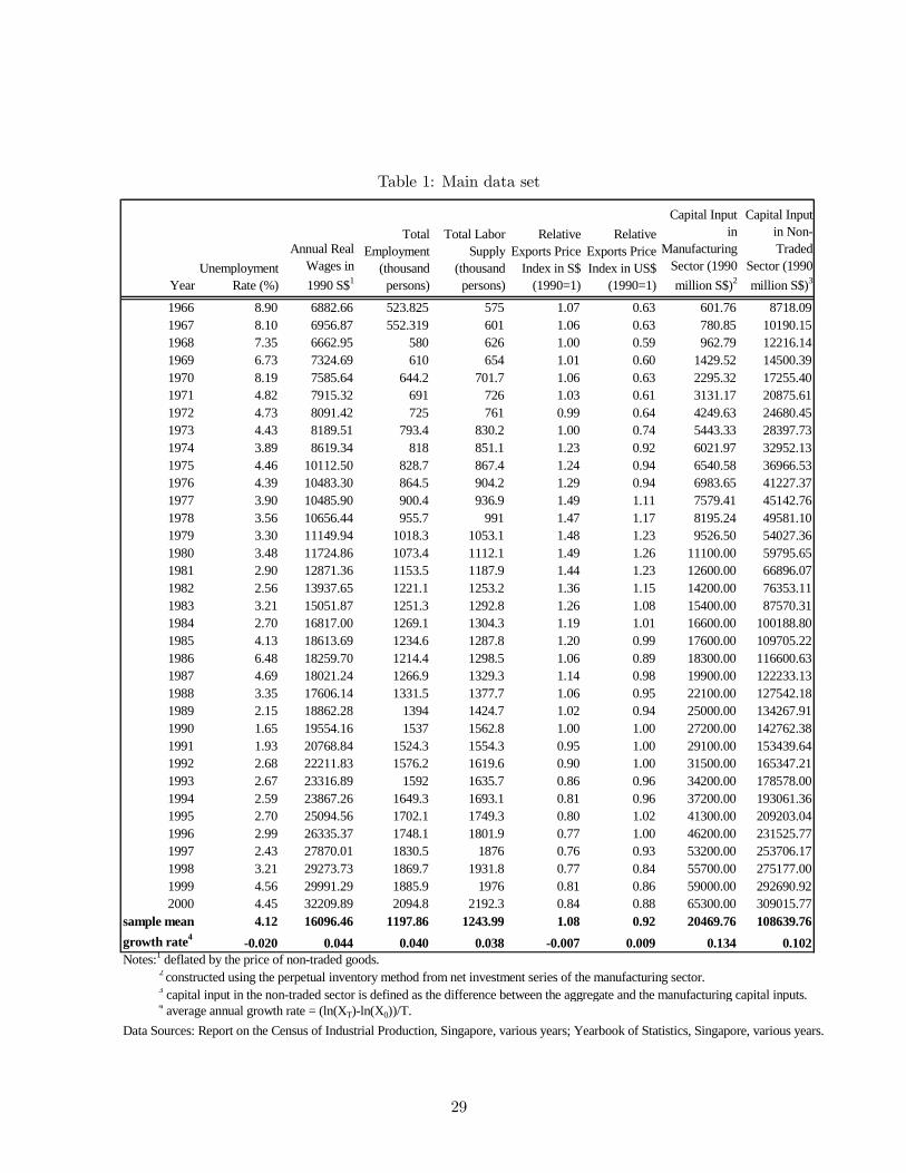
Table 1: Main data set

YearUnemployment

Rate (%)

Annual Real Wages in

1990 S$1

Total Employment

(thousand persons)

Total Labor Supply

(thousand persons)

Relative Exports Price

Index in S$ (1990=1)

Relative Exports Price Index in US$

(1990=1)

Capital Input in

Manufacturing Sector (1990

million S$)2

Capital Input in Non-Traded

Sector (1990

million S$)3

1966 8.90 6882.66 523.825 575 1.07 0.63 601.76 8718.091967 8.10 6956.87 552.319 601 1.06 0.63 780.85 10190.151968 7.35 6662.95 580 626 1.00 0.59 962.79 12216.141969 6.73 7324.69 610 654 1.01 0.60 1429.52 14500.391970 8.19 7585.64 644.2 701.7 1.06 0.63 2295.32 17255.401971 4.82 7915.32 691 726 1.03 0.61 3131.17 20875.611972 4.73 8091.42 725 761 0.99 0.64 4249.63 24680.451973 4.43 8189.51 793.4 830.2 1.00 0.74 5443.33 28397.731974 3.89 8619.34 818 851.1 1.23 0.92 6021.97 32952.131975 4.46 10112.50 828.7 867.4 1.24 0.94 6540.58 36966.531976 4.39 10483.30 864.5 904.2 1.29 0.94 6983.65 41227.371977 3.90 10485.90 900.4 936.9 1.49 1.11 7579.41 45142.761978 3.56 10656.44 955.7 991 1.47 1.17 8195.24 49581.101979 3.30 11149.94 1018.3 1053.1 1.48 1.23 9526.50 54027.361980 3.48 11724.86 1073.4 1112.1 1.49 1.26 11100.00 59795.651981 2.90 12871.36 1153.5 1187.9 1.44 1.23 12600.00 66896.071982 2.56 13937.65 1221.1 1253.2 1.36 1.15 14200.00 76353.111983 3.21 15051.87 1251.3 1292.8 1.26 1.08 15400.00 87570.311984 2.70 16817.00 1269.1 1304.3 1.19 1.01 16600.00 100188.801985 4.13 18613.69 1234.6 1287.8 1.20 0.99 17600.00 109705.221986 6.48 18259.70 1214.4 1298.5 1.06 0.89 18300.00 116600.631987 4.69 18021.24 1266.9 1329.3 1.14 0.98 19900.00 122233.131988 3.35 17606.14 1331.5 1377.7 1.06 0.95 22100.00 127542.181989 2.15 18862.28 1394 1424.7 1.02 0.94 25000.00 134267.911990 1.65 19554.16 1537 1562.8 1.00 1.00 27200.00 142762.381991 1.93 20768.84 1524.3 1554.3 0.95 1.00 29100.00 153439.641992 2.68 22211.83 1576.2 1619.6 0.90 1.00 31500.00 165347.211993 2.67 23316.89 1592 1635.7 0.86 0.96 34200.00 178578.001994 2.59 23867.26 1649.3 1693.1 0.81 0.96 37200.00 193061.361995 2.70 25094.56 1702.1 1749.3 0.80 1.02 41300.00 209203.041996 2.99 26335.37 1748.1 1801.9 0.77 1.00 46200.00 231525.771997 2.43 27870.01 1830.5 1876 0.76 0.93 53200.00 253706.171998 3.21 29273.73 1869.7 1931.8 0.77 0.84 55700.00 275177.001999 4.56 29991.29 1885.9 1976 0.81 0.86 59000.00 292690.922000 4.45 32209.89 2094.8 2192.3 0.84 0.88 65300.00 309015.77

sample mean 4.12 16096.46 1197.86 1243.99 1.08 0.92 20469.76 108639.76

growth rate4-0.020 0.044 0.040 0.038 -0.007 0.009 0.134 0.102

Notes:1 deflated by the price of non-traded goods. 2 constructed using the perpetual inventory method from net investment series of the manufacturing sector. 3 capital input in the non-traded sector is defined as the difference between the aggregate and the manufacturing capital inputs. 4 average annual growth rate = (ln(XT)-ln(X0))/T.

Data Sources: Report on the Census of Industrial Production, Singapore, various years; Yearbook of Statistics, Singapore, various years.

29

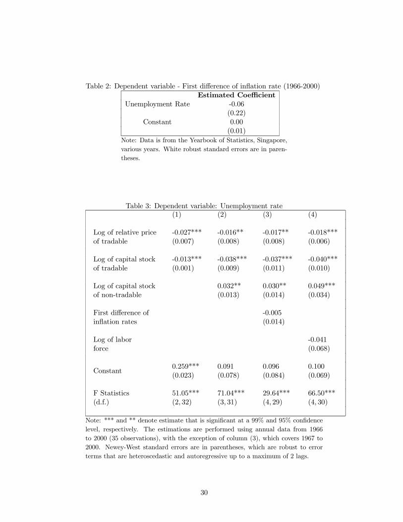
Table 2: Dependent variable - First difference of inflation rate (1966-2000)Estimated Coefficient

Unemployment Rate -0.06(0.22)

Constant 0.00(0.01)

Note: Data is from the Yearbook of Statistics, Singapore,various years. White robust standard errors are in paren-theses.

Table 3: Dependent variable: Unemployment rate(1) (2) (3) (4)

Log of relative priceof tradable

-0.027***(0.007)

-0.016**(0.008)

-0.017**(0.008)

-0.018***(0.006)

Log of capital stockof tradable

-0.013***(0.001)

-0.038***(0.009)

-0.037***(0.011)

-0.040***(0.010)

Log of capital stockof non-tradable

0.032**(0.013)

0.030**(0.014)

0.049***(0.034)

First difference ofinflation rates

-0.005(0.014)

Log of laborforce

-0.041(0.068)

Constant0.259***(0.023)

0.091(0.078)

0.096(0.084)

0.100(0.069)

F Statistics(d.f.)

51.05***(2, 32)

71.04***(3, 31)

29.64***(4, 29)

66.50***(4, 30)

Note: *** and ** denote estimate that is significant at a 99% and 95% confidencelevel, respectively. The estimations are performed using annual data from 1966to 2000 (35 observations), with the exception of column (3), which covers 1967 to2000. Newey-West standard errors are in parentheses, which are robust to errorterms that are heteroscedastic and autoregressive up to a maximum of 2 lags.

30

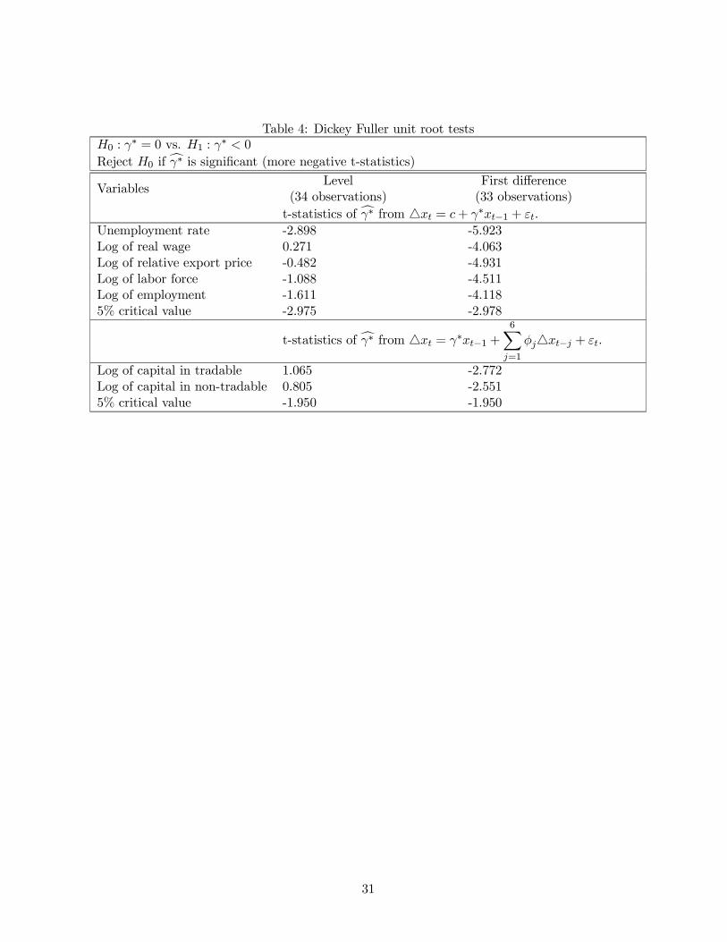
Table 4: Dickey Fuller unit root testsH0 : γ∗ = 0 vs. H1 : γ∗ < 0Reject H0 if γ∗ is significant (more negative t-statistics)

VariablesLevel

(34 observations)First difference(33 observations)

t-statistics of γ∗ from xt = c+ γ∗xt−1 + εt.

Unemployment rate -2.898 -5.923Log of real wage 0.271 -4.063Log of relative export price -0.482 -4.931Log of labor force -1.088 -4.511Log of employment -1.611 -4.1185% critical value -2.975 -2.978

t-statistics of γ∗ from xt = γ∗xt−1 +6

j=1

φj xt−j + εt.

Log of capital in tradable 1.065 -2.772Log of capital in non-tradable 0.805 -2.5515% critical value -1.950 -1.950

31

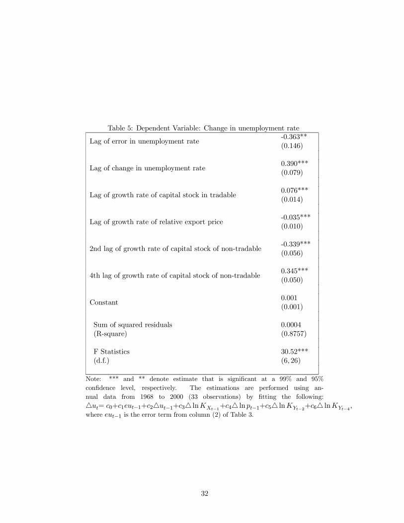
Table 5: Dependent Variable: Change in unemployment rate

Lag of error in unemployment rate-0.363**(0.146)

Lag of change in unemployment rate0.390***(0.079)

Lag of growth rate of capital stock in tradable0.076***(0.014)

Lag of growth rate of relative export price-0.035***(0.010)

2nd lag of growth rate of capital stock of non-tradable-0.339***(0.056)

4th lag of growth rate of capital stock of non-tradable0.345***(0.050)

Constant0.001(0.001)

Sum of squared residuals(R-square)

0.0004(0.8757)

F Statistics(d.f.)

30.52***(6, 26)

Note: *** and ** denote estimate that is significant at a 99% and 95%confidence level, respectively. The estimations are performed using an-nual data from 1968 to 2000 (33 observations) by fitting the following:ut= c0+c1eut−1+c2 ut−1+c3 lnKXt−1+c4 ln pt−1+c5 lnKYt−2+c6 lnKYt−4,

where eut−1 is the error term from column (2) of Table 3.

32

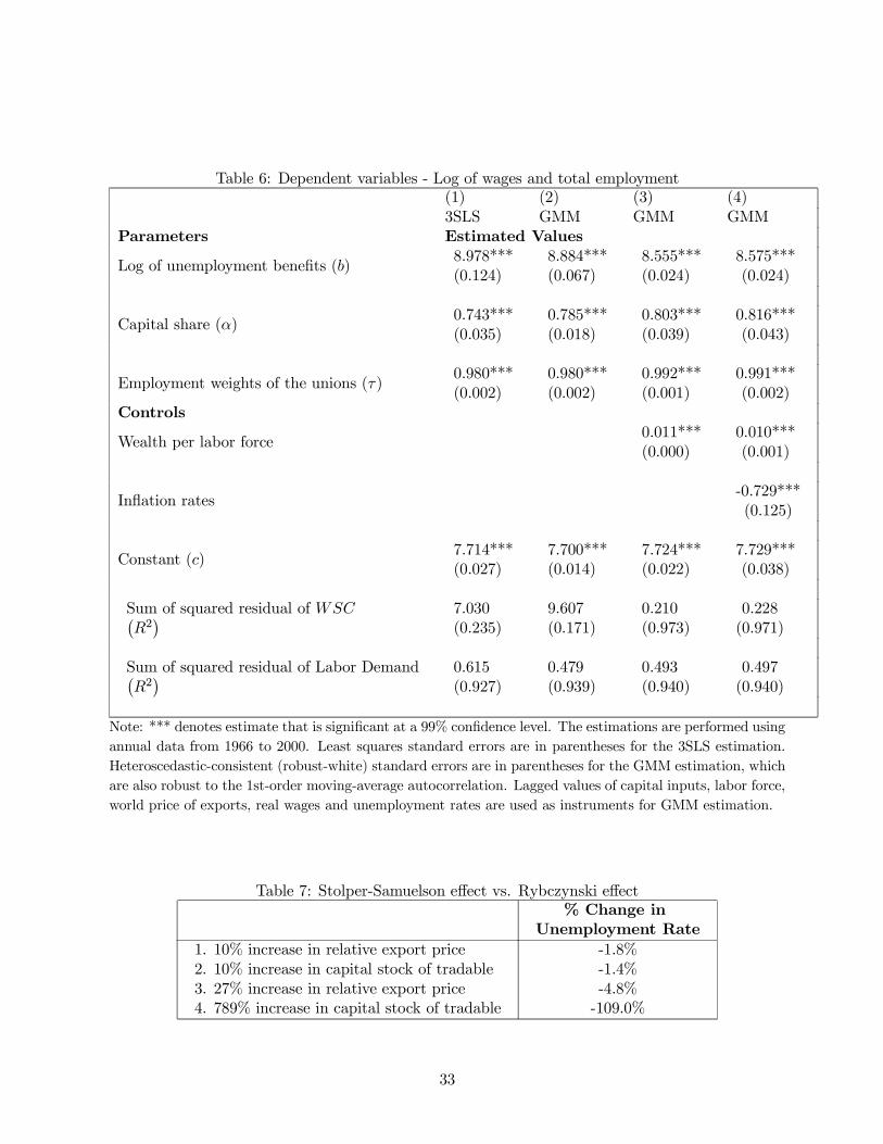
Table 6: Dependent variables - Log of wages and total employment(1) (2) (3) (4)3SLS GMM GMM GMM

Parameters Estimated Values

Log of unemployment benefits (b)8.978***(0.124)

8.884***(0.067)

8.555***(0.024)

8.575***(0.024)

Capital share (α)0.743***(0.035)

0.785***(0.018)

0.803***(0.039)

0.816***(0.043)

Employment weights of the unions (τ)0.980***(0.002)

0.980***(0.002)

0.992***(0.001)

0.991***(0.002)

Controls

Wealth per labor force0.011***(0.000)

0.010***(0.001)

Inflation rates-0.729***(0.125)

Constant (c)7.714***(0.027)

7.700***(0.014)

7.724***(0.022)

7.729***(0.038)

Sum of squared residual of WSCR2

7.030(0.235)

9.607(0.171)

0.210(0.973)

0.228(0.971)

Sum of squared residual of Labor DemandR2

0.615(0.927)

0.479(0.939)

0.493(0.940)

0.497(0.940)

Note: *** denotes estimate that is significant at a 99% confidence level. The estimations are performed usingannual data from 1966 to 2000. Least squares standard errors are in parentheses for the 3SLS estimation.Heteroscedastic-consistent (robust-white) standard errors are in parentheses for the GMM estimation, whichare also robust to the 1st-order moving-average autocorrelation. Lagged values of capital inputs, labor force,world price of exports, real wages and unemployment rates are used as instruments for GMM estimation.

Table 7: Stolper-Samuelson effect vs. Rybczynski effect% Change in

Unemployment Rate1. 10% increase in relative export price2. 10% increase in capital stock of tradable3. 27% increase in relative export price4. 789% increase in capital stock of tradable

-1.8%-1.4%-4.8%-109.0%

33

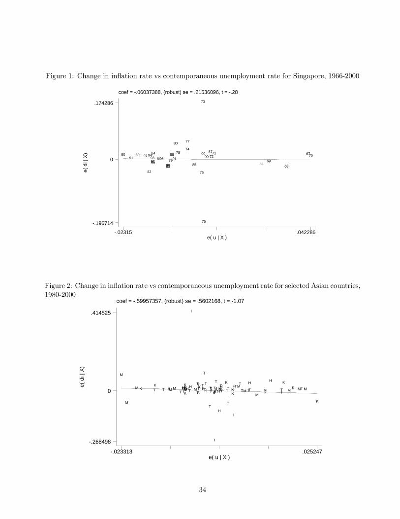
Figure 1: Change in inflation rate vs contemporaneous unemployment rate for Singapore, 1966-2000

coef = -.06037388, (robust) se = .21536096, t = -.28e(

di |

X)

e( u | X )-.02315 .042286

0

-.196714

.174286

9091

89 97

82

94939295

84

8196

839879

8801

80

7874

77

85

76

73

00

75

998772

71

8669

68

6770

Figure 2: Change in inflation rate vs contemporaneous unemployment rate for selected Asian countries,1980-2000

coef = -.59957357, (robust) se = .5602168, t = -1.07

e( d

i | X

)

e( u | X )-.023313 .025247

0

.414525

-.268498

M

M

M K TK

T KM MT

THTTHK

KKKMH

TH

I

M

T

T

TTKTK

TK

T

TT

T

I

T

TTTT

K

I

TTK

T

KTH

H

KTTTMT

K

T

T

T IKK

I

THTM

T

TM TT

H

MKM

H

TT

K

MK MT M

K

34

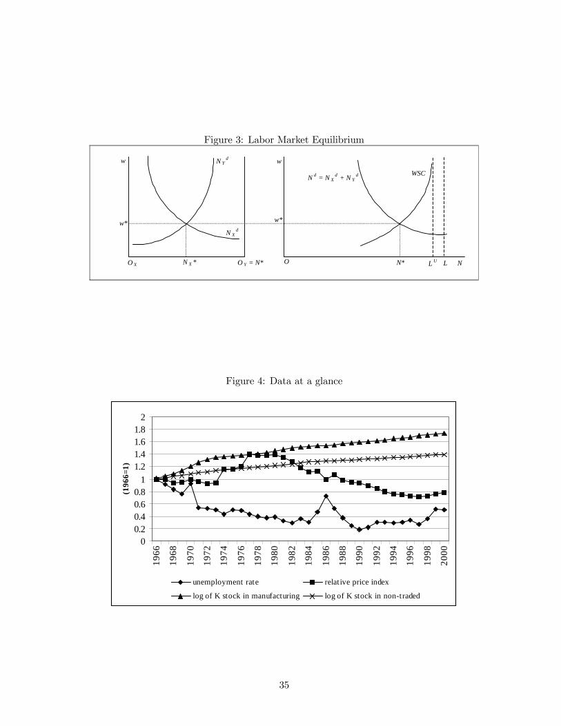
Figure 3: Labor Market Equilibrium

N Yd

N Xd

O X O Y = N* N*

w* w*

w w

WSCN d = N X

d + N Yd

NN X * L U LO

Figure 4: Data at a glance

00.20.40.60.8

11.21.41.61.8

2

1966

1968

1970

1972

1974

1976

1978

1980

1982

1984

1986

1988

1990

1992

1994

1996

1998

2000

(196

6=1)

unemployment rate relat ive price index

log of K stock in manufacturing log of K stock in non-traded

35

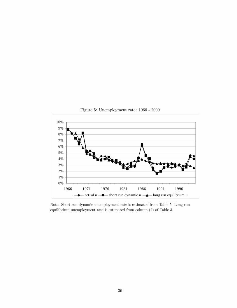
Figure 5: Unemployment rate: 1966 - 2000

0%

1%

2%

3%

4%

5%

6%

7%

8%

9%

10%

1966 1971 1976 1981 1986 1991 1996

actual u short run dynamic u long run equilibrium u

Note: Short-run dynamic unemployment rate is estimated from Table 5. Long-runequilibrium unemployment rate is estimated from column (2) of Table 3.

36