Embed Size (px)
Citation preview

TMD DISCUSSION PAPER NO. 96
TRADE AND THE SKILLED-UNSKILLED WAGE GAP IN A
MODEL WITH DIFFERENTIATED GOODS
Karen Thierfelder U.S. Naval Academy and International Food Policy Research
Institute (IFPRI) and
Sherman Robinson International Food Policy Research Insitute (IFPRI)
Trade and Macroeconomics Division International Food Policy Research Institute
2033 K Street, N.W. Washington, D.C. 20006, U.S.A.
July 2002
TMD Discussion Papers contain preliminary material and research results, and are circulated prior to a
full peer review in order to stimulate discussion and critical comment. It is expected that most Discussion Papers
will eventually be published in some other form, and that their content may also be revised. This paper is
available at http://www.cgiar.org/ifpri/divs/tmd/dp.htm
Abstract
There is a continuing debate about whether international trade is responsible for the observed skilled-unskilled wage gap. In this paper we present a general equilibrium trade model with differentiated goods. We begin with an analytical model and show how changes in relative factor returns can be decomposed into changes in commodity prices, changes in the trade balance, and changes in the factor endowment Then we use a computable general equilibrium (CGE) trade model calibrated to the U.S. economy in 1982 to analyze the effects of these shocks, as well as technology changes, observed in the U.S. in the 1980's. (JEL F11,F14, F15)

Table of Contents
I. The 1-2-2-3 Model ......................................................................................................................4 II. Properties of the 1-2-2-3 Model..................................................................................................9
A. Implications for the Stolper-Samuelson Theorem .........................................................9 B. Implications for the Rybczynski Theorem....................................................................12 C. Trade-Balance Effects ...................................................................................................12
III. Properties of the Decomposition Equation .............................................................................14 IV. Multi-Sector Model of the U.S. Economy in 1982..................................................................16 V. Conclusions..............................................................................................................................23 References......................................................................................................................................26
List of Discussion Papers...............................................................................................................45
1
Trade and the Skilled-Unskilled Wage Gap in a Model with Differentiated Goods
By, Karen Thierfelder and Sherman Robinson1
There is a continuing debate about the role of changes in trade on the evolution of relative
wagesCparticularly the skilled-unskilled wage gap. In the 1980's, the wage gap widened considerably in
the United States, and there was an active literature on the roles of trade, technology, and changes in
labor supplies, particularly due to migration and education, in explaining these changes. The empirical
models used to analyze the links fall into two broad groups: (1) partial-equilibrium models of the labor
market, focusing on changes in the supply and demand of labor by skill category, and (2) general
equilibrium trade models linking domestic factor returns to changes in world prices and the
composition of trade.1
Labor economists use Afactor content@ models to analyze how changes in the composition of
demand for goods feeds back into domestic factor markets in a partial-equilibrium framework. Recent
studies include Adrian Wood (1994, 1995, 1998), Jeffrey Sachs and Howard Shatz (1994), and George
J. Borjas et al. (1992, 1996). These models start by assuming that unskilled-labor-intensive imports
displace unskilled-labor-intensive domestic production. Using input-output data, they identify the shifts
in labor demand arising from changes in the structure of demand for goods, which are then assumed
to affect equilibrium wages in labor markets.2 In this framework, labor economists find that any
worsening of the U.S. trade deficit contributes to the widening wage gap because the increase in
unskilled-labor-intensive imports relative to capital-intensive and skill-intensive exports will reduce the
demand for unskilled labor.3
Trade economists, using the Heckscher-Ohlin-Samuelson (HOS) model, look for links
between commodity prices and factor prices. From the Stolper-Samuelson Theorem, in a world with

2
all goods tradable, one would expect changes in world commodity prices to generate large changes in
domestic factor prices4 The Factor-Price Equalization Theorem makes an even stronger statement:
assuming identical tastes and technology in all countries, free trade in commodities will lead to
identical factor prices internationally, regardless of differing factor endowments across countries Ca
result often cited by protectionist pressure groups in the North. Finally, the Rybczynski Theorem
shows that, with unchanged commodity prices, changes in factor endowments will lead to a magnified
change in the structure of production and trade, but no change in relative wages. Trade theory would
thus tend to focus attention on commodity prices and trade rather than changes in the skill-
composition of the domestic labor supply.5
There are serious theoretical problems in reconciling the labor-market and trade-theory
approaches. J. David Richardson (1995, p.35) identifies the challenge: AIn short, the work that needs to
be done in this area will bridge the gap between international and labor economics.@ Some progress
has been made in that direction. For example, Matthew J. Slaughter (1999) summarizes the differences
between the two perspectives and describes the implications of each approach for the elasticity of labor
demand. George Johnson and Frank Stafford (1999) describe what labor economists might find useful
in trade theory.
In this paper, we present a theoretical model that can capture many of the differences between
the approaches of trade and labor economists. We start with Ronald W. Jones (1974), who examines
the role of non-traded goods in the HOS model. We extend Jones to include imperfect substitutability
between traded and non-traded goods, and the links between product markets and factor markets. The
model also includes the balance of trade and the real exchange rate, which supports analysis of how
changes in the trade balance affect factor markets. We show that, in this model, changes in relative
wages can be decomposed into effects arising from changes in: (1) relative factor supplies, (2) relative

3
prices, and (3) the trade balance. In contrast to the Afactor content@ approach, we show that increases
in the trade deficit should reduce the gap between skilled and unskilled wages in a developed country
such as the U.S.
After describing the links between trade and wages in our theoretical model, we then use a
CGE trade model calibrated to the U.S. economy in 1982 to analyze the links between changes in
relative wages and changes in trade, technology, factor supplies, and the trade balance.6 There are 15
sectors, with a focus on manufacturing sectors. This aggregation is useful to analyze the effect of trade
on U.S. wages because relevant imports from developing countries are primarily in the unskilled-labor-
intensive manufacturing sectors. There are four labor categories in the model. We use the model for
two applications.7 First, we show the importance of trade in affecting relative wages by simulating the
counterfactual: what would U.S. wages be in the absence of trade with developing countries?8 Second,
we use the model to decompose the impact on relative wages of changes in international prices, the
trade balance, and the supply of unskilled labor of the order of magnitude observed in the 1980's. We
find that a small endowment change can generate a dramatic change in the wage gap and that a large
change in international prices generates a small change in the wage gap. Our results are consistent with
those from empirical trade models which use regression analysis and find that trade is not responsible
for the observed widening of the wage gap between skilled and unskilled labor. We then consider the
role of biased technological change, which can have large effects.
The remainder of the paper is organized as follows. First, we present the theoretical model and
discuss its properties. We conclude with a decomposition equation showing that changes in relative
wages arise from changes in relative prices, relative factor supplies, and the trade balance. We then
use an empirical CGE model of the U.S. economy in 1982 to show how relative wages respond to
4
changes in relative prices, relative factor supplies, and the trade balance of the order of magnitude
observed in the 1980's. Our conclusions follow.
I. The 1-2-2-3 Model
We present a general equilibrium trade model with non-traded goods which are imperfect
substitutes with traded goods.9 This theoretical model underlies a large class of single- and multi-
country, applied, computable general equilibrium (CGE) trade models. Computable general
equilibrium (CGE) models use the assumption, originally described in Paul S. Armington (1969), that
goods are differentiated by country of origin and that imports and domestic goods are imperfect
substitutes in demand.10 Such CGE models have been used extensively to analyze the effect of free
trade agreements as well as trade and domestic policy reform issues in both developed and developing
countries.11
Our analytical model closely follows Jones (1974) who incorporates a non-traded good into the
2x2x2 HOS framework. We expand upon Jones by (1) exploring the factor market linkages, which he
did not; (2) treating the non-traded good as a semi-traded good which is an imperfect substitute in
consumption for the imported good; and (3) adding the balance of trade. The result we call the 1-2-
2-3 model C one country, two production activities, two inputs, and three commodities. A version of
this model without factor markets, the 1-2-3 model (one country, two production activities, and three
commodities), was first described in de Melo and Robinson (1989). They specified explicit functional
forms for the aggregate utility function (constant elasticity of substitution, CES) and the production
possibility frontier (constant elasticity of transformation, CET).12
The economy produces two goods, E and D. The good E is exported and is not consumed
domestically. The good D is consumed domestically. Imports, M, represent a third commodity which
5
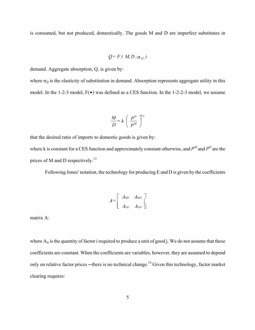
is consumed, but not produced, domestically. The goods M and D are imperfect substitutes in
demand. Aggregate absorption, Q, is given by:
where σQ is the elasticity of substitution in demand. Absorption represents aggregate utility in this
model. In the 1-2-3 model, F($) was defined as a CES function. In the 1-2-2-3 model, we assume
that the desired ratio of imports to domestic goods is given by:
where k is constant for a CES function and approximately constant otherwise, and PM and PD are the
prices of M and D respectively.13
Following Jones= notation, the technology for producing E and D is given by the coefficients
matrix A:
where Aij is the quantity of factor i required to produce a unit of good j. We do not assume that these
coefficients are constant. When the coefficients are variables, however, they are assumed to depend
only on relative factor prices Cthere is no technical change.14 Given this technology, factor market
clearing requires:
) ; D M,( F = Q Qσ
PP k =
DM
M
D Qσ
AA
AA = A
LDLE
KDKE

6
where K and L are aggregate supplies of capital and labor.
In competitive equilibrium, unit costs will equal market prices:
where WK and WL are the Awages@ of capital and labor and PE and PD are output prices.
To close this model, we require an equation linking exports and imports. We assume that the
balance of trade is given by:
where Φ is a parameter giving the ratio of import expenditures to export earnings. This specification
extends the standard HOS model, allowing the balance of trade to affect consumption, production,
and factor returns. When Φ is one, trade is balanced, with export earnings exactly equaling import
costs Cas in the usual HOS model. The trade balance (the value of exports minus imports in world
prices) equals (1 - Φ) times export earnings. An increase in Φ implies a worsening of the trade
balance.
Assuming that the country is Asmall@ so that we can assume world prices, PM and PE, are
fixed, the model is complete. There are seven equations for seven endogenous variables: Q, E, D, M,
WK, WL, and PD. Unlike the HOS model, one of the commodity prices is endogenous.
L = D A + E A
K = D A + E A
LDLE
KDKE
P = W A + W A
P = W A + W A
DLLDKKD
ELLEKKE
E P = MP EM Φ

7
We demonstrate how the endogenous variables, particularly relative wages, change in
response to changes in the prices of the traded goods (PE and PM), factor supplies (K and L), and the
balance of trade (Φ). We use Jones=s (1965) notation to describe endowment shares (λij, the share of
the total supply of factor i used in sector j) and value added shares (θij, the share of factor i in total
income generated in sector j). We assume that the export good is relatively capital intensive so the
determinants of matrices of both λij, and θij, denoted as ||λ and ||θ , are positive (and less than
one). The elasticity of transformation between E and is given by Ω. It is a function of the endowment
shares and the elasticities of substitution between labor and capital in production of goods E and D.15
The model reduces to four relationships in changes in relative prices, production, and
demand. The first is the link between changes in relative prices and relative wages along the contract
curve underlying the production possibility frontier.
In the standard HOS model, where both goods are tradeable and their prices are set in world
markets, this equation demonstrates the Stolper-Samuelson Theorem. Relative wages depend only
on relative prices and, since 1 < θ , the change in relative wages is greater than the change in
relative prices Cthe model incorporates the magnification effect.
Second, movements along the production possibility frontier are determined both by changes
in relative prices and changes in relative factor endowments.
( ) ( ) P - P
1 = W - W DE
LK θ

8
This equation demonstrates the Rybczynski Theorem. Since 1 < λ , with unchanged prices,
changes in relative factor endowments will have a magnified effect on relative production.16
The demand side of the model involves D and M rather than D and E. Log differentiating
equation 2 yields:
This equation shows how relative demand for M and D changes with changes in relative
prices.
Finally, the supply and demand sides are linked through the balance-of-trade equation. Log
differentiating equation 6 yields:
The changes in relative prices of D and E can be expressed as a function of changes in
exogenous world prices, factor endowments, and the balance of trade:
In this model, when world prices are fixed, PD is the relative price of nontraded (semi-
tradable) goods to traded goods, and represents the real exchange rate.17 In the general case, there is
( ) ( ) ( ) P - P + L - K
1 = D - E DE Ωλ
( ) ( ) P - P - = D - M DMQ σ
( ) Φ - P - P = M - E EM
( ) ( ) ( )
Φ
Ω K - L
1 + - ) P - P( ) 1 - (
+ 1 = P - P
MEQ
Q
DE λ
σσ

9
effectively a different real exchange rate for imports and exports. Equation 11 refers to domestically
produced goods supplied to domestic and world markets, and describes how the economy moves
along the production possibility frontier as a function of changes in world prices, the balance of
trade, and factor endowments.
Changes in relative wages can be expressed in terms of changes in world prices, the balance
of trade, and factor endowments:
This is the fundamental result from the 1-2-2-3 model. In contrast to the HOS model, when
nontraded goods are included, changes in relative wages depend not only on changes in world prices,
but also on changes in factor endowments and the balance of trade. Furthermore, the model can
accommodate factor-biased technological change, something the standard HOS model cannot. In
our framework, factor-biased technological change operates like a change in the endowment and
therefore affects relative wages.
II. Properties of the 1-2-2-3 Model
A. Implications for the Stolper-Samuelson Theorem
As the elasticity of substitution in consumption, σ Q , goes to infinity, the last two terms in
brackets in equation 12 go to zero. In the limit, the remaining term in world prices reduces to:
( ) ( ) ( )
Φ
Ω K - L
1 + - ) P - P( ) 1 - (
+ 1 = W - W
MEQ
QLK
λ
σσθ

10
which corresponds to equation 7 with P = PMD since D and M are now perfect
substitutes. This is exactly the HOS model, with changes in relative wages depending only on
changes in world prices, and the Stolper-Samuelson Theorem again applies. The HOS model can
thus be seen as a special case of the 1-2-2-3 model when imports and domestic goods are perfect
substitutes.
When there is no change in factor supplies and the balance of trade, equation 12 reduces to:
Since Ω is positive, the second term in this expression is always less than one. The result is
that the magnification effect in the Stolper-Samuelson Theorem is reduced. The larger is the
transformation elasticity Ω and the closer is the elasticity of substitution in demand to one, the
weaker is the link between changes in prices and changes in relative wages.
When the elasticity of substitution equals one, the right-hand side goes to zero and changes
in world prices have no effect on relative wages. One way to see what is going on is to consider the
country=s offer curve, which shows the relationship between exports (on the horizontal axis) and
imports (on the vertical axis) as world prices change. As Jaime de Melo and Sherman Robinson
(1989) show, when 1 = Qσ the country=s offer curve becomes vertical. In that case, as the world
price of imports changes, expenditure on imports remains fixed nominally and hence, with a fixed
export price, real exports do not change.18 Hence, there is no movement along the production
( ) ( ) P - P
1 = W - W ME
LK θ
( ) ( )( ) ) P - P(
+ 1 -
1 = W - W ME
Q
QLK
Ωσσ
θ

11
possibility frontier, and relative wages do not change. The link between changes in world prices and
changes in relative wages is completely broken.
When 1 > Qσ , from equation 11, an increase in the price of imports leads to an increase in
the price of D, which corresponds to an appreciation of the real exchange rate. The offer curve
slopes upwards. When imports become more expensive, it is worthwhile to produce more of the
domestic substitute, moving resources away from the production of exports. The volume of trade
declines and, from equation 14, the relative wage of capital falls. Such a situation might characterize
a developed country when the price of its imports rise on world markets. The sign of the results is
the same as in the HOS model, but the magnification effect is weakened or eliminated.
When 1 < Qσ , M and D are weak substitutes. In this case, an increase in the world price of M
leads to a decrease in the price of D relative to E, which is a depreciation of the real exchange rate.
Production of D declines and exports increase. In effect, the country depreciates in order to shift
resources into exports, increasing export earnings in order to pay for the more expensive, but
essential, imports. The offer curve is backward bending. This situation is characteristic of
developing countries which have to undergo a structural adjustment program in the face of an
adverse terms-of-trade shock (for example, a large increase in the price of oil). In this case,
changing a commodity price has the opposite effect on wages than would be predicted by the HOS
model. In a developing country exporting labor-intensive goods, where 0 < θ , an increase in the
price of imports will lead to an increase in the wage of labor relative to capital, while the HOS
model would predict a decrease. The 1-2-2-3 model seems much more realistic in this case.

12
B. Implications for the Rybczynski Theorem
To consider the application of the Rybczynski Theorem in the 1-2-2-3 model, consider the
relationship between the change in domestic relative prices as factor endowments change when
world prices and the balance of trade do not change (equation 11). Substitute the resulting
expression for P - PDE into equation 8. The result is an expression relating the change in the
structure of production as a function of the change in factor endowments, all other exogenous
variables held constant:
As with the Stolper-Samuelson Theorem, this equation reduces to the HOS version (equation
8, the Rybczynski Theorem) as a special case in the limit when the elasticity of substitution (σ Q )
goes to infinity. In general, however, the magnification effect in the Rybczynski Theorem is
ameliorated. Since Ω is greater than zero, the term in brackets is less than one. The greater is Ω and
the lower is σ Q , the weaker is the link between changes in factor endowments and changes in the
structure of production. Unlike the Stolper-Samuelson Theorem, there is no sign reversal when
1 < Qσ .
C. Trade-Balance Effects
One view of the effect of changes in the balance of trade on relative wages is that a
worsening in the trade balance (increasing Φ) leads to increased imports which displace domestic
( ) ( ) ( ) L - K +
1 = D - E Q
Q
Ωσσ
λ

13
production of low-skill, labor-intensive goods (D), and hence should widen the wage gap. Borjas et
al. (1992), using the factor-content approach, compute the net implicit contribution of the trade
deficit to the supply of labor by different skill categories. They conclude (p. 214): AThe annual
increase in implicit labor supply due to the mid- and late-1980's trade deficit in manufactures was on
the order of 1.5 percent for the economy as a whole and 6 percent for the manufacturing sector.@
They then analyze the impact of these shifts on wages in a partial-equilibrium analysis of the labor
markets, concluding that A. . . from 15 to 25 percent of the 11 percentage point rise in the earnings of
college graduates relative to high school graduates from 1980 to 1985 can be attributed to the
massive increase in the trade deficit over the same period.@
In equation 12, however, an increase in Φ will lead to a narrowing of the wage gap, since the
sign of the coefficient on Φ is negative. There is a serious conflict between the 1-2-2-3 model and
the labor-market approach. The problem is a conflict between partial- and general-equilibrium
models. The labor-market approach assumes that increased imports due to the worsening of the
balance of trade will Adisplace@ domestic production of labor-intensive goods. However, increasing
Φ implies that absorption will rise since the worsening trade balance shifts the consumption
possibility frontier out, even though the production possibility frontier stays the same. Consumers
have more to spend and, since D is a normal good, they will demand more D as well as more M. The
effect will be to increase the relative price of D, as shown in equation 11, shifting resources away
from E to produce more D. The increase in PD represents an appreciation of the real exchange rate
and the model demonstrates the Dutch disease.19 The production of E declines, D expands, and the
relative wage gap narrows.20
14
III. Properties of the Decomposition Equation
Equation 12 can be used to decompose the relative contributions of changes in world prices,
the balance of trade, and factor endowments to changes in relative factor returns. This
decomposition is at the heart of the policy debate about the causes of the widening of the skilled-
unskilled wage gap in the U.S. The 1-2-2-3 model can be used as the organizing framework for
detailed empirical work, using both econometric analysis and simulation models. Here, we calibrate
the parameters for the 1-2-2-3 model, using data for the U.S. in 1982, to show the magnitude of the
coefficients in equation (21).21 The aggregate data for the U.S. from the Economic Report of the
President do not differentiate labor by skill category so we use the two inputs capital and labor. To
include skilled-labor in this framework, one can assume that it is a complement to capital in
production.
Value and endowment shares for the export and the domestic sector appear in table 1.22 Note
that the value share to capital in the export sector is greater than the value share to labor in that
sector, indicating that the export sector is capital intensive. Likewise, the endowment share of
capital in the export sector exceeds the endowment share of labor in the export sector. We assume
the elasticity of substitution of factors in production ( σσ DE , ) is 0.1.
Table 2 reports the elasticity of import substitution, (σ Q ) , assumed to be 3.0. Using the
assumed elasticities and the observed value and endowment shares, we compute the transformation
elasticity. The resulting coefficients for the price, trade balance, and endowment terms in equation
21 are given in Table 2.
Note first that the Stolper-Samuelson magnification effect is nearly eliminated. The
coefficient on the price term is 1.11, which implies that relative wages change only slightly more

15
than relative prices. Second, the size of the coefficient for the endowment term, 5.51, is much larger.
Not only do changes in endowments have a direct effect on relative wages, the effect is magnified.
There is a large scope for factor-market and endowment effects in this type of trade model.
Finally, the trade balance (or Dutch disease) effect is smaller and of opposite sign than the
price effect. The relative size of the trade balance effect is set by the choice of the import
substitution elasticity. For a value of three, the effect is exactly half the value of the price effect. A
given percent worsening of the trade balance will offset half of a comparable change in relative
world prices. In the short run, one might well assume a lower import substitution elasticity, and so
expect a larger offset.
Data for the changes in relative prices, the change in the trade balance, and the change in the
relative supply of labor to capital also appear in table 2, calculated for the time periods 1980-1985
and 1986-1990. The trade balance shows the most dramatic changes over the two time periods. It
increased 31 percent in the early 1980's and declined 21 percent from 1986 to 1990. Consistent with
an increase in the trade deficit, the price of exports relative to the price of imports increased from
1980 to 1985. Using the computed coefficients for the decomposition equation and data for the U.S.
in 1980-1990, we find that the return to capital relative to labor increased ten percent from 1980
to1985. It declined seven percent from 1986 to 1990. Despite the large increase in the trade deficit
from 1980-1985, which has a negative coefficient in the decomposition equation, the wage gap
increased over that period.
We find that the calculated coefficients in the decomposition equation are sensitive to
parameter values. For example, when the import substitution parameter increases, the size of both
the endowment and trade-balance effects decreases and the price effect increases. As expected, the

16
model moves toward the standard HOS model as the import substitution elasticity increases, but
contrary to the HOS model, the endowment term remains important. Even when the substitution
elasticity reaches a value of 32, the coefficient on the endowment term is around one.
We also consider the sensitivity of the coefficients in the decomposition equation to initial
trade shares. In the standard HOS model, the trade share is irrelevant Cit matters only whether a
good is tradable, not how much is traded. In the 1-2-2-3 model, the response of relative wages to
changes in endowments is very sensitive to the trade share. The coefficients on the price and trade-
balance terms level off as the trade share reaches 20 percent, while the coefficient on endowments
falls steadily. At a trade share of 40 percent, the size of the endowment effect is close to the price
effect. Labor economists and trade theorists share equal billing in countries with high trade shares.
Finally, we consider the sensitivity to the transformation elasticity, Ω, which is computed
from the production elasticities, endowment shares, and value added shares (see equation 15). We
find that as the transformation elasticity increases, the magnitudes of all three effects decrease. The
endowment effect is relatively more important the lower is the transformation elasticity, but its
coefficient remains significantly larger than the others for all values of Ω. Our sensitivity analysis
suggests that the focus of labor economists on supply and demand in factor markets is well
grounded, even in a trade-focused general equilibrium model.
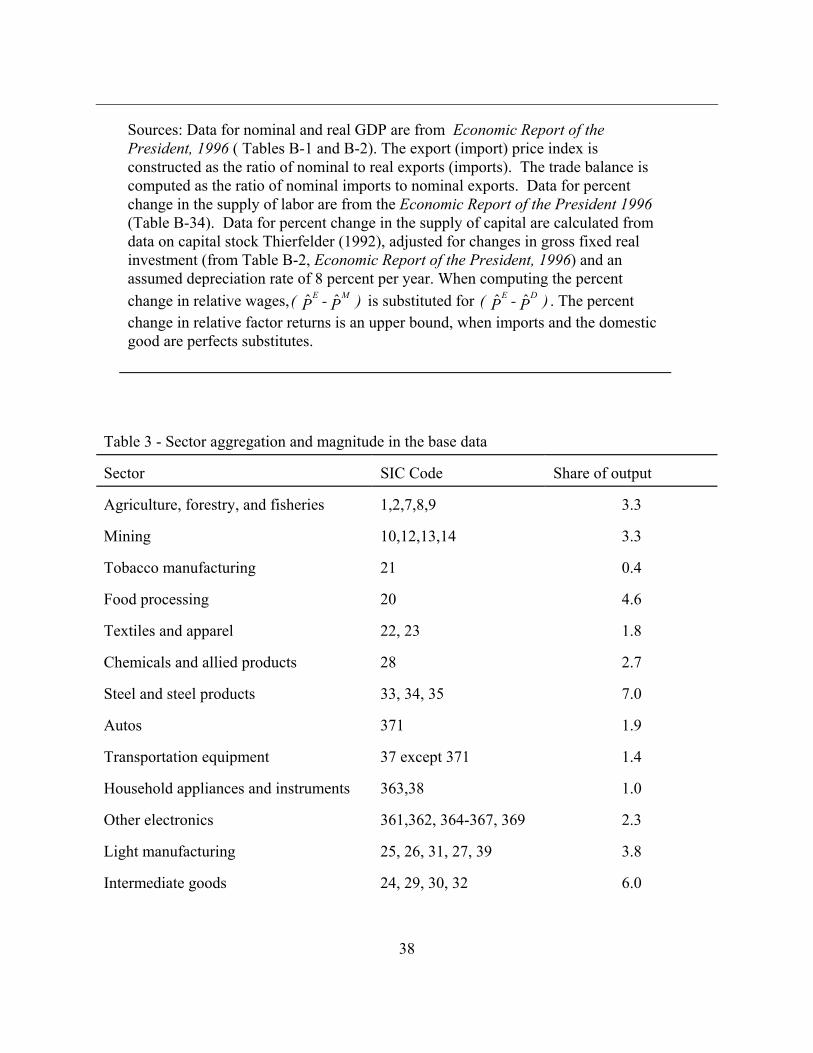
IV. Multi-Sector Model of the U.S. Economy in 1982 To
get a better perspective of the U.S. wage gap in the 1980's, we use a multi-sector version of the 1-2-
2-3 model, calibrated to the U.S. economy in 1982.23 There are 15 sectors in the computable general
equilibrium (CGE) model, with an emphasis on manufacturing sectors which had high import shares
of consumption during that time period (see table 3).24

17
There are four types of labor B professional, technical support, semi-skilled, and low-skilled.
These categories are aggregates of the occupations defined by the Standard Occupation
Classification in the U.S. Census (see table 4). The data matrices of employee compensation and the
number of full time equivalents by both sector and occupation are constructed from two sources.
The March 1987 Current Population Survey provides information on the share of income and the
share of workers by occupation for each industry. The shares are used to distribute both the
employee compensation and the number of full time equivalents for each industry as provided in the
Survey of Current Business.25
Table 5 provides information on the structure of the U.S. economy in 1982. In general, the
manufacturing sectors have a high share of imports in consumption, particularly sectors such as
autos, consumer electronics, light manufacturing, and textiles. There is some evidence of two-way
trade in sectors such as steel, autos, household appliances and consumer electronics for which both
the share of exports in production and imports in consumption are high.
Value added shares (θ ij ) and endowment shares (λ ij ) are given in tables 6 and 7. Textiles,
steel, autos, and light manufacturing have high value added shares for unskilled labor. These sectors
also have high import shares in consumption.
In the multi-sector CGE model, goods are produced for both intermediate and final demand.
Intermediate input demands are taken from the U.S. input-output table. Production requires primary
factors (labor, land, and capital) with CES value-added functions and intermediate inputs with fixed
input-output coefficients. With this production structure, we must account for both the direct factor
use and the indirect factor use which arises through demand for intermediate inputs. In table 8, we
report direct and indirect factor coefficients, measured as the share of the factor per unit of output.

18
We also report the factor content of the domestic good, imports, and exports. As a developed
country, the unskilled-labor content of U.S. imports exceeds the unskilled labor content of U.S.
exports. Likewise the skilled-labor content of U.S. exports (professional labor) exceeds the skilled-
labor content of U.S. imports.26
The relationship between trade changes, production changes, and changes in factor returns
are more complicated in the multi-sector model, compared to the analytical model in which only two
goods are produced. At first glance, one may think that links in the decomposition equation (21)
would break down in a multi-sector model because there are more goods than factors. However, we
impose the structure of the analytical model sector-by-sector, with imperfect substitution in
consumption between the imported and the domestic variety of each good (Armington elasticity) and
imperfect substitution in production between the exported and the domestic variety (constant
elasticity of transformation, CET, elasticity).
DeMelo and Robinson (1989) extend the 1-2-3 (one country, two production activities, and
three goods) to the multi-sector model. Here, we discuss extensions that are relevant to factor
market linkages in the 1-2-2-3 model, which they do not discuss. First, the multi-sector model, by
construction, adds strong separability in production. The Armington and CET functions by sector
allow some adjustment to price changes to take place within a sectorBan increase in sectoral exports,
for example, can be met by either a reduction in sales to the domestic market or by an increase in
production. There is less need for output structure to change in the multi-sector model than in the
analytical model, since the model allows both exports and imports in the same sector (two-way
trade). As a result, factor intensity differences by sector matter less. The multi-sector model thus

19
has a bias against finding a big trade effect because of separability by sector.27 When the Armington
and CET elasticities are low, the multi-sector model behaves more like the analytical model.
A final important difference between the multi-sector and the analytical model is that
consumer preferences differ by sector. For example, in the U.S. model, the highest consumer
expenditure shares are on high-wage services, low-wage services, and food. These sectors have
different factor intensities and trade shares so, a priori, it is not clear how a change in income will
affect factor returns. In the analytical model, when income increased, consumption of both imports
and domestic goods increased, increasing the production of the domestic good and the return to
unskilled labor, which the domestic good is assumed to use intensively.
First, we use the CGE model to consider the question, Awhat would the structure of U.S.
wages be, but for imported manufactured goods from developing countries?@ We simulate a 50
percent reduction in the quantity of manufactured imports.28 Consistent with other empirical studies
of the links between trade and wages, we find a very small impact on wages. In the base model, the
ratio of the professional wage to the unskilled wage is 1.60. That ratio reduces slightly to 1.59
following a 50 percent reduction in manufactured imports in the central elasticity case. A negligible
change, given the magnitude of the import shock.
Next, we use the model for three comparative static simulations based on the decomposition
equation (21). The magnitudes of the shocks are constructed to reflect changes observed in the U.S.
in the 1980's. We consider a 50 percent reduction in the world prices of imports, an increase in the
trade balance by $200 billion (from essentially zero), and a 5 percent decrease in the supply of
unskilled labor. 29 We also consider the sensitivity of our results to the elasticity of substitution
between imports and domestic goods in consumption. In our discussion of the Stolper-Samuelson

20
theorem we note that the sign on the link between trade price shocks and the wage gap depends upon
whether or not the elasticity of substitution is greater or less than one.
In the central case, we find that the price and labor market changes in the multi-sector model
are consistent with the changes predicted in the analytical model. A 50 percent decline in the price of
imported manufactured goods increases the wage gap between professional (skilled) and unskilled
workers. However, the change is small given the magnitude of the price shock: the ratio of
professional wages to unskilled wages is 1.60 in the base and 1.61 following the reduction of import
prices. When imports and domestic goods are poor substitutes, the wage ratio declines slightly,
to1.59. As shown in the discussion of the Stolper-Samuelson results for the analytical model, when
the elasticity of substitution between imports and domestic goods is less than one, the sign on the
link between commodity prices and factor returns changes. When imports and domestic goods are
highly substitutable, so it is easier for imports to displace domestic goods in consumption, the wage
ratio increases further to 1.63.30
In all scenarios, an increase in the trade deficit has only a slight impact on the wage ratio,
the highest value being 1.61 in the high Armington elasticities case. However, the analytical model
predicts that when the trade deficit worsens, there is an increase in absorption, and the wage gap
narrows. In that model, consumers spend more on the imported good (M) and the domestic good
(D). As production of D increases, demand for unskilled labor increases. In the multi-sector model,
the same mechanism is at work, but the links are more complicated because there are 15 different
goods to consume, each with different factor intensities. The consumer has the highest expenditure
shares for low-wage services, high-wage services, and processed food. The high-wage service sector

21
has a very high direct and indirect professional labor coefficient (table 8) suggesting that when it
expands, it puts upward pressure on the professional wages, increasing the wage gap.
Finally, a reduction in the supply of unskilled labor reduces the wage substantially, to 1.54,
regardless of the Armington elasticity. This change is consistent with predictions from the analytical
model. The change is in the correct direction and is large, given that the labor supply only contracted
5 percent. In contrast, a 50 percent reduction in the price of imports has a much smaller impact on
relative wages. The model suggests that endowment changes have a dramatic effect on the wage
gap.
In contrast, an endowment change does not affect factor prices in the HOS model, where
only price changes and sector-biased technical change can influence the wage gap. As Richardson
(1995, p. 42) notes, AThe [trade-wage] debate increasingly and properly isolates trade prices and
sectoral total factor productivity differences as the causes of long-run factor-price movements.
Trade volumes are correspondingly treated endogenously. Neutral and factor-augmenting
technological change is seen to be just like factor-supply change, with innocuous impacts on factor
prices.@ In our framework, factor-biased technological change will affect the wage gap because it
operates like an endowment change. Trade can have a big effect on wages when it induces factor-
biased technological change. Wood (1994,1995) makes this argument, noting that imports of
unskilled-labor-intensive goods from developing countries induce Adefensive innovation@ by firms in
developed countries as they use new production methods that economize on unskilled labor.
Next, we cumulate the effects of the three shocks to provide a historical decomposition of the
wage gap for the U.S. in the 1980's. The trade deficit, coupled with the import price shock, widens
the wage ratio to from 1.61, with the import price shock alone, to 1.62. However, the net effect of

22
the import price shock, the change in the trade deficit, and the change in the supply of unskilled
labor, reduces he wage ratio to 1.56. This result is consistent with our earlier discussion of the
effects of each shock individually. However, it is not consistent with the observed data. For
example, James Harrigan and Rita A. Balaban (1999, figure 2) report that the in the U.S., the ratio
of college graduate to high school graduate average weekly wage went from 1.52 in 1980 to 1.7 in
1985. Similarly, Robert E. Baldwin and Glen Cain (1999, table 1) report the ratio of workers with 13
or more years of education to workers with 12 or fewer years of education with respect to wages
rose from 1.38 in 1980 to 1.50 in 1987.
The contrast between our simulated wage ratio and the actual wage ratio suggests that our
model omits another shock which affected the relative wage in the U.S. during the 1980s. Many
researchers attribute the increase in the wage gap to technological change.31 In our simulation model,
one can compute the technology shock needed to generate the observed wage gap, given the
observed price, trade balance, and endowment shock. One can incorporate sector-biased total factor
productivity growth, consistent with the approach that Lisandro Abrego and John Whalley (2000)
and others who follow the HOS model use. Or, one can find the factor-biased productivity shock,
similar to the change Wood (1998) describes, that is consistent with the observed wage ratio and
other shocks. In our model, we can accommodate either type of technology shock. This is in
contrast to the HOS model in which factor-biased technological progress operates like an
endowment shock and has no effect on factor prices when commodity prices are determined in large
world markets.
We find that, given the observed price, trade balance, factor endowment, and relative wage
changes, factor-biased technological change in which skilled labor becomes more productive must
23
have increased by 40 percent in the U.S. in the 1980s. Similarly, total factor productivity in the
sectors that use unskilled labor relatively intensively would have had to increase by 64 percent,
given the observed price, trade balance, factor endowment and relative wage changes.
Alternatively, it may be that the labor market is segmented. Many studies of the skilled-
unskilled wage gap in the U.S. focus on manufacturing sectors. In the short term, the unskilled
workers in the manufacturing sectors may be unable to move into the services sectors which have a
much higher share of domestic goods in consumption than the other sectors in the economy (see
table 5) and therefore are less vulnerable to trade shocks. We consider the implications of this view
of the labor market and find that trade shocks have a much stronger effect on wages when the labor
markets are segmented. For example, when the import price of manufactured goods falls 50 percent,
the ratio of the payment to skilled workers to unskilled workers in the non-services sectors increases
from 1.5 to 1.62 (see table 9). A combined shock of the price decline and the trade deficit increase
the ratio to 1.76 and both the trade and labor supply shocks generate a wage gap of 1.69. These
results suggest that in the short term, when it may be difficult for unskilled workers to move out of
manufacturing sectors, trade shocks can have a strong impact on the wage ratio.
V. Conclusions
The debate about the impact of changes in world prices and trade on relative wages in
developed countries has been strongly influenced by neoclassical trade theory, especially the
Heckscher-Ohlin-Samuelson (HOS) model. In this general-equilibrium model, changes in factor
supplies do not affect relative wages. We extend the analytic HOS model to include semi-tradable
goods, thus capturing the fact that imports and domestic goods are imperfect substitutes in
production.

24
Our extended analytic model incorporates the theoretical properties of a large body of
empirical CGE models used for trade policy analysis. We show that in this class of models, the
change in relative factor prices depends not only on changes in commodity prices, as explained in
the Stolper-Samuelson theorem, but also on changes in both factor endowments and the balance of
trade. Our model provides a unifying framework for the trade-wage debate.
Analysis with an archetype model, patterned after the U.S. in 1982, indicates that changes in
relative wages are more sensitive to changes in factor endowments than to changes in world prices
or the trade balance. Not only is there room for labor economists, they have a prominent role.
However, Stolper-Samuelson effects become more important as the trade share increases, which
brings trade economists back into the picture. This result from the 1-2-2-3 model is intuitively
appealing and contrary to the standard HOS model, where trade shares are irrelevant. Finally,
changes in the trade balance do affect relative wages, but in the opposite direction from that derived
from factor-content analysis, which assumes increased imports displace domestic production. The 1-
2-2-3 model captures the general-equilibrium feedback from increasing aggregate absorption, which
is ignored in the partial-equilibrium approach.
The results from the empirical multi-sector model are consistent with other studies of the
links between trade and wages. Increased trade, which reduces the price of unskilled-labor-intensive
import goods in developed countries, is responsible for very little of the observed wage gap. When
we simulate a reduction in imports, we find only a slight reduction in the wage gap. Conversely,
when we reduce the price of imported manufactured goods in the U.S. by approximately the change
observed during the 1980'=s, the wage gap increases slightly. In addition, changes in the trade
balance, and hence changes in absorption, also only have a small effect on the wage gap, despite the

25
observed large increase in the trade deficit during the 1980's. However, endowment changes do
have large effects on the wage gap. Our results suggest an indirect route for trade to influence wages.
When trade encourages factor-biased technological trade, it will dramatically influence the wage
gap.

26
References
Abrego, Lisandro and John Whalley.AThe Choice of Structural Model in Trade-Wage Decompositions.@ Review of International Economics, 2000, 8(3), pp. 462-477.
Armington, Paul S. AA Theory of Demand for Products Distinguished by Place of Production.@ IMF Staff Papers, 1969, Vol. 16, pp. 159-178.
Baldwin, Robert E. and Glen Cain. AShifts in Relative U.S. Wages: The Role of Trade, Technology and Factor Endowments,@ Review of Economics and Statistics, 2000, 82(4), pp. 580-595.
Bhagwati, Jagdish and Vivek H. Dehejia. AFreer Trade and Wages of the Unskilled CIs Marx Striking Again?@ in Bhagwati and Kosters eds., Trade and Wages. Washington, D.C.: American Enterprise Institute, 1994.
Borjas, George J,. Richard B. Freeman, and Lawrence F. Katz. AOn the Labor Market Effects of Immigration and Trade,@ in George J. Borjas and Richard B. Freeman, eds., Immigration and the Work Force. Chicago: University of Chicago and NBER, 1992, pp. 245-69.
Borjas, George J., Richard B. Freeman, and Lawrence F. Katz. ASearching for the Effect of Immigration on the Labor Market.@ Unpublished, Harvard University and NBER, presented to the American Economic Association Meetings, January 5-7, 1996, San Francisco, California, 1996.
Burfisher, Mary E. and Elizabeth A. Jones, eds. Regional Trade Agreements and U.S. Agriculture, Economic Research Service, AER No. 771. Washington, DC: U.S. Department of Agriculture, 1998.
Burtless, Gary. AInternational Trade and the Rise in Earnings Inequality.@ Journal of Economic Literature, June 1995, Vol. 33, pp. 800-816.
Deardorff, Alan V. AFactor Prices and the Factor Content of Trade Revisited: What's the Use?@ Journal of International Economics, 2000, Vol. 50, p. 73-90.
Deardorff, Alan and Dalia Hakura . ATrade and Wages: What are the Questions?@in Bhagwati and Kosters eds., Trade and Wages. Washington, D.C.: American Enterprise Institute, 1994..
Deardorff, Alan and Robert W. Staiger (1988). AAn Interpretation of the Factor Content of Trade.@ Journal of International Economics, Vol. 16, pp. 93-107.

27
Devarajan, Shantayanan, Jeffrey D. Lewis, and Sherman Robinson. AExternal Shocks, Purchasing Power Parity, and the Equilibrium Real Exchange Rate.@ World Bank Economic Review, January 1993, 7(1), pp. 45-63.
Devarajan, Shantayanan, Jeffrey D. Lewis, and Sherman Robinson. APolicy Lessons from Trade-Focused Two-Sector Models.@ Journal of Policy Modeling, 1990, 12( 4), pp. 625-657.
Feenstra, Robert C. and Gordon H. Hanson. AGlobal Production Sharing and Rising Inequality: A Survey of Trade and Wages,@ National Bureau of Economic Research (Cambridge, MA) Working Paper No.8372, 2001.
Francois, Joseph F. and Clinton R. Shiells, eds. Modeling Trade Policy: Applied General Equilibrium Assessments of North American Free Trade. Cambridge: Cambridge University Press, 1994.
Francois, Joseph F. and Douglas Nelson. ATrade Technology, and Wages: General Equilibrium Mechanics.@ Economic Journal, 1998 Vol. 108, pp. 1483-1499.
Freeman, Richard B. AAre Your Wages Set in Bejing?@ Journal of Economic Perspectives 1995, 9(3), pp. 15-32.
Harrigan, James and Rita A. Balaban. AU.S. Wage Effects in General Equilibrium: The Effects of Prices, Technology, and Factor Supplies, 1963-1991.@ National Bureau of Economic Research (Cambridge, MA) Working Paper No. 6981, 1999.
Johnson, George and Frank Stafford. AThe Labor Market Implications of International Trade,@ in Orley
Ashenfelter and David Cards, eds., Handbook of Labor Economics, Vol. 3b, Amsterdam: Elsevier, 1999, pp. 2215-2288.
Jones, Ronald W. AThe Structure of Simple General Equilibrium Models.@ Journal of Political Economy, 1965, 73(6), pp. 557-72.
Jones, Ronald W. ATrade with Non-Traded Goods: The Anatomy of Interconnected markets.@ Economica, May 1974, Vol. 41, pp. 121-138.
Jones, Ronald W. AInternational Trade, Real Wages and Technical Progress: The Specific Factors Model.@ International Review of Economics and Finance, 1996, 5(2), pp. 113-24.
Krugman, Paul R. ATechnology, Trade and Factor Prices.@ Journal of International Economics, 2000, Vol. 50., pp.51-71.
Krugman, Paul R. AGrowing World Trade: Causes and Consequences@ Brookings Papers on Economic Activity, Microeconomics, 1995, Vol. 1, pp. 327-377.
Krugman, Paul R. and Robert Lawrence. ATrade, Jobs and Wages.@National Bureau of Economic Research (Cambridge, MA) Working Paper No. 4478, 1993.

28
Lawrence, Robert Z. and Matthew J. Slaughter. AInternational Trade and American Wages in the 1980s:
Giant Sucking Sound or Small Hiccup?@ Brookings Papers on Economic Activity, Microeconomics, 1993, Vol. 2, pp. 161-226.
Leamer, Edward E. AIn Search of Stolper-Samuelson Linkages between International Trade and Lower Wages,@ in Susan M. Collins, ed., Imports, Exports and the American Worker. Washington D.C.:Brookings Institution Press, 1998, pp. 141-203.
Leamer, Edward E. AWhat's the Use of Factor Contents?@ National Bureau of Economic Research (Cambridge, MA) Working Paper No. 5448, 1996.
Winters, L. Alan, ed. The Uruguay Round and the Developing Countries, Cambridge: Cambridge University Press, 1996.
Melo, Jaime de. AComputable General Equilibrium Models for Trade Policy Analysis in Developing Countries: A Survey.@ Journal of Policy Modeling, 1988, Vol. 10, pp. 469-503.
Melo, Jaime de, and Sherman Robinson. AProduct Differentiation and the Treatment of Trade in Computable General Equilibrium Models of Small Countries.@ Journal of International Economics, 1989, 7(1), pp. 45-63.
Richardson, J. David. AIncome Inequality and Trade: How to Think, What to Conclude.@ Journal of Economic Perspectives, 1995, 9(3), pp. 33-55.
Robinson, Sherman. AMultisectoral Models,@ in H. Chenery and T.N. Srinivasan, eds., Handbook of Development Economics, Volume 2. Amsterdam: Elsevier Science Publishers, 1989.
Sachs, Jeffrey and Howard Shatz.. ATrade and Jobs in U.S. Manufacturing.@ Brookings Papers on Economic Activity, 1994, Vol. 1, pp. 1-84.
Salter, Wilfred. AInternal and External Balance: The Role of Price and Expenditure Effects.@ Economic Record, 1959, Vol. 35, pp. 226-38.
Shiells, Clinton R. and Kenneth Reinert. AArmington Models and Terms of Trade Effects: Some Econometric Evidence for North America.@ Canadian Journal of Economics, 1993, Vol 26, pp. 299-316.
Swan, T. AEconomic Control in a Dependent Economy.@ Economic Record, 1960, Vol. 36, pp. 51-66.
Slaughter, Matthew J. AWhat are the Results of Product-Price Studies and What Can We Learn from Their Differences?@ in Robert C. Feenstra, ed., The Impact of International Trade on Wages. Chicago: University of Chicago Press, 2000, pp. 129-170.

29
Slaughter, Matthew J. AGlobalization and Wages: A Tale of Two Perspectives.@ The World Economy, 1999, 22(5), pp. 609-629.
Tyers, Rod and Yongzheng Yang. ATrade with Asia and Skill Upgrading: Effects on Labor in the Older Industrial Countries.@ Weltwirtschaftliches Archiv, 1997, 133(3), pp. 383-417.
Williamson, Jeffrey G. AGlobalization and Inequality Then and Now: The Late 19th and Late 20th Centuries Compared.@ Unpublished, Harvard University, presented to the American Economic Association Meetings, January 5-7, 1996 San Francisco, California, 1995..
Wood, Adrian. AGlobalisation and the Rise in Labour Market Inequalities,@ Economic Journal, 1998, Vol. 108, pp. 1463-1482.
Wood, Adrian. AHow Trade Hurt Unskilled Workers.@ Journal of Economic Perspectives, 1995, 9(3), pp. 57-80.
Wood, Adrian. North-South Trade, Employment, and Inequality. Oxford: Clarendon Press, 1994.

30
* Thierfelder: Economics Department, U.S. Naval Academy, 589 McNair Rd., Annapolis, MD
21402 (e-mail: [email protected]); Robinson: Director, Trade and Macroeconomics Division,
International Food Policy Research Institute, 2033 K Street, N.W., Washington D.C. 20006 (e-
mail: [email protected]).
1. See J. David Richardson (1995), Richard B. Freeman (1995), Matthew J. Slaughter (2000), and
Robert C. Feenstra and Gordon H. Hanson (2001) for surveys of the models. Gary Burtless
(1995) and Jeffrey G. Williamson (1995) provide historical overviews.
2. Trade economists also have views about the factor content model. Alan Deardorff (2000) and
Alan Deardorff and Robert W. Staiger (1988), using an analytical trade model, find that the factor
content of trade can be used to indicate the effects of trade on relative factor prices. Paul R.
Krugman (2000) notes that trade theorists were wrong to reject the factor content approach. In
contrast, Edward E. Leamer (1996) argues that the link between factor contents and factor returns
is ambiguous.
3.George J. Borjas et al. (1992, p.214), not that Afrom 15 to 25 percent of the 11 percentage point
rise in the earnings of college graduates relative to high school graduates from 1980 to 1985 can be
attributed to the massive increase in the trade deficit over the same period.@
4.As Leamer (1998, pp.146-147) notes, neoclassical trade theory implies that Aprices are set on the
margin. Y What matters is whether or not the marginal unskilled worker is employed in the
apparel sector, sewing the same garments as a Chinese worker whose wages are one-twentieth of

31
the U.S. level.@
5.See Leamer (1998), Robert E. Baldwin and Glenn Cain (2000), and James Harrigan and Rita
A. Balaban (1999) for regression analysis of trade relationships derived from a general
equilibrium trade model. In general, trade economists find that the links between trade and
wages are small empirically. Leamer (1998) notes that the 1970s was the Stolper-Samuelson
decade, and that there was a 4 percent mandated reduction per year in unskilled-wages.
6.Rod Tyers and Yongzheng Yang (1997) also use an applied general equilibrium model to
examine the effects of East Asian openness and growth on developed-country factor markets.
Harringan and Balaban (1999) use a regression model to analyze wage inequality in the U.S.
7. We provide one Acomplete general equilibrium story@ that Krugman (1995, p.344) notes Ahas
been absent from the debate.@ He presents a stylized general equilibrium model with a Aset of
ballpark parameters@ (p. 329) to evaluate the impact of trade with Newly Industrializing Economies
(NIE) on wages in developed countries. He finds that trade the observed increase in trade with
NIE countries can be associated with fairly small wage changes. We use a CGE model calibrated to
actual U.S. data to answer similar questions.
8. Krugman (2000) and Alan Deardorff and Dalia Hakura (1994) note that this is the appropriate
counterfactual when looking at the effect of trade on wages.
9.The model is an extension of the Salter-Swan model in which the non-traded good is not
substitutable with the traded good. See Wilfred Salter (1959) and T. Swan (1960) for the original
model.

32
10. Paul S. Armington (1969) used this specification in estimating import demand functions. Many
empirical studies support this specification. For example, Clinton R. Shiells and Kenneth Reinert
(1993) find low import substitution elasticities for the U.S., Canada, and Mexico, suggesting that it
is important to characterize imported and domestic goods as semi-tradable.
11.Many surveys of CGE trade models are available: NAFTA (Joseph F. Francois and Clinton R.
Shiells, 1994), regional trade agreements and agriculture (Mary E. Burfisher and Elizabeth A.
Jones, 1998), and the Uruguay Round (Will Martin and L. Alan Winters, 1996). Sherman
Robinson (1989) and Jaime de Melo (1988) describe the application of these models to
development issues.
12.Shantayanan Devarajan et al. (1990, 1993) explore the properties of the model in detail,
extending it to include tariffs and taxes, and also use the same basic framework to analyze issues
concerning the appropriate definition of the equilibrium real exchange rate.
13.In the general case, we ignore income effects and assume the absorption function is well
behaved (e.g. homothetic, convex, and twice-differentiable).
14.We also assume that both sectors use both factors in equilibrium, so there are no corner
solutions.
15.An appendix with the formal derivation is available from the authors upon request.
16.Equations 16 and 17 present results for relative wages and production. When only one price
changes, one can show that one wage goes up while the other falls (Stolper-Samuelson).
Similarly, one can show that, with a change in one factor endowment, one output goes up while

33
the other falls (Rybczynski).
17.This equation is equivalent to the equation for the real exchange rate in the 1-2-3 model
derived in Devarajan et al. (1993), with the addition of a term for changes in factor endowments.
18.The model is characterized by Lerner symmetry. It does not matter whether world export or
import prices change. In the cases discussed below, for expositional convenience, we will start
from a change in the world price of imports, assuming export prices are fixed.
19.The Dutch disease occurs when an increase in availability of foreign exchange (arising, say,
from the discovery of oil in the North Sea) worsens the trade balance and generates a real
appreciation of the exchange rate, increasing imports, and reducing production of tradables.
20.Jagdish Bhagwati andVivek H. Dehejia (1994) also criticize Borjas et al. but from the
perspective of the HOS model, arguing that changes in endowments should have no effect on
relative wages. Leamer (1996, pp. 11-12) considers a model with nontradables and notes that:
AAn external deficit raises the demand for nontradables and may or may not affect wages.@ In a
footnote, he worries about different causes of a change in the deficit, and how they might affect
relative wages.
21.Lisandro Abrego and John Whalley (2000) use a similar empirical approach and calibrate a
two sector, two factor general equilibrium model for the UK in 1990. They use data on the
observed changes in wages and prices to solve for the sector-biased technological change
consistent with the data. This simulation allows them to decompose the effects of trade and
technology on wage changes. We first derive the decomposition equation from the analytical
34
model and use the data to determine the magnitude of the coefficients in the decomposition
equation. We then use a much more detailed CGE model calibrated to the U.S. in 1982 to
simulate the effects of the observed changes in relative prices, the trade balance and the relative
endowment on changes in relative wages.
22.Production and trade data are from the U.S. National Income and Product Accounts. To
aggregate sectors, we treat all sectors which are net exports as the export sector. Those
remaining sectors which are net imports are aggregated into the domestic sector.
23.Krugman (2000) argues that there is a need for a computable general equilibrium model,
calibrated for the U.S. economy with commodity detail, to better explore the general equilibrium
linkages. He presents a stylized model, in which both goods are traded, calibrated to Aball park
parameters,@ similar to our approach in section III.
24.A detailed description of the model and data is available from the authors upon request.
25.The Survey of Current Business is a better source of data on income because it provides
information on employee compensation which indicates the factor cost from the producer=s
perspective. Likewise, the number of full time equivalents, found in the Survey of Current
Business, is a better indication of factor use than the labor data in the Current Population Survey.
As a result, only the occupation detail is taken from the Current Population Survey.
26.We find there is no Leontief paradox in the data.
27.This separability implies the need for disaggregation in the multi-sector model. Then, there
will tend to be more specialization, with less observed two-way trade by sector.

35
28.Since we use constant elasticity of substitution (CES) import demand equations, it is not
possible for imports to equal zero. Instead we reduce imports dramatically.
29.Data for the change in the relative price of imports are from Harrigan and Balaban (1999,
figure 5) in which they report a 45 percent decline in the price of unskilled-labor-intensive
tradable goods. This is an upper bound on the price change; at the other extreme, studies report
that there is little evidence of a reduction in the prices of unskilled-labor intensive goods in the
U.S. (for example, Robert Z. Lawrence and Matthew J. Slaughter, 1993). Harriagan and Balaban
(1999, table 2) report a 12 percent decline in the supply of workers with 11 or fewer years of
education for the 1980-1990 period; and Baldwin and Cain (2001, table 1) report the average
annual percentage decline for this group to be 2.3 percent from 1980-87. Based on this data, we
consider the effects of a 5 percent decline in the supply of unskilled labor. The trade balance is
taken directly from data reported in the Economic Report of the President. It represents
75percent of the value of exports in the base model and 6.4percent of real GNP.
30.The wage response to price shocks is sensitive to the elasticity of substitution among inputs in
production. In the scenarios reported here, we assume an elasticity of 1.5 in all sectors.
Sensitivity analysis shows that for lower elasticities of substitution, which adds curvature to the
transformation frontier, the magnitude of the change in the wage gap for the given price shocks
is bigger.
31.For a discussion of the role of technological progress in the trade-wage debate, see Krugman
(2000), Baldwin and Cain (2000), Leamer (1998), Josehp F. Francois and Douglas Nelson
(1998) and Wood (1998).

36
Table 1- Archetype data and parameters for U.S.
Exports (E) Domestic (D)
Sum
Output 10 90 100 Capital (K) 8 47 55 Labor (L) 2 43 45 Value shares (θ) K 0.80 0.52 L 0.20 0.48 Factor shares (λ) K 0.15 0.85 1.00 L 0.04 0.96 1.00

37
K/L substitution elasticity ( ) , DE σσ 0.10 0.10
The archetype data are based on data for the U.S. economy in the 1980s from the Economic Report of the President, 2000. GDP is normalized at 100, output and factor prices are normalized to one. Nominal exports were approximately 10% of the value of nominal GDP during the 1980s.
Table 2 - Relative wage change equation
Coefficients
Value Import substitution elasticity ( ) Qσ
3.00
Transformation elasticity (Ω)
3.46
Determinant θ
0.28
Determinant λ
0.11
Relative wage change equation: ( ) ) K - L ( 5.51 + 0.56 - ) P - P ( 1.11 = W - W
DELK
Φ Decomposition of relative wage changes
1980-1985
1986-1990
) P - P ( ME
0.22
-0.07
Φ
0.31
-0.21
) K - L (
0.01
-0.02
) W - W ( LK
0.10
-0.07
38
Sources: Data for nominal and real GDP are from Economic Report of the President, 1996 ( Tables B-1 and B-2). The export (import) price index is constructed as the ratio of nominal to real exports (imports). The trade balance is computed as the ratio of nominal imports to nominal exports. Data for percent change in the supply of labor are from the Economic Report of the President 1996 (Table B-34). Data for percent change in the supply of capital are calculated from data on capital stock Thierfelder (1992), adjusted for changes in gross fixed real investment (from Table B-2, Economic Report of the President, 1996) and an assumed depreciation rate of 8 percent per year. When computing the percent change in relative wages, ) P - P ( ME is substituted for ) P - P ( DE . The percent change in relative factor returns is an upper bound, when imports and the domestic good are perfects substitutes.
Table 3 - Sector aggregation and magnitude in the base data
Sector
SIC Code
Share of output
Agriculture, forestry, and fisheries
1,2,7,8,9
3.3
Mining
10,12,13,14
3.3
Tobacco manufacturing
21
0.4
Food processing
20
4.6
Textiles and apparel
22, 23
1.8
Chemicals and allied products
28
2.7
Steel and steel products
33, 34, 35
7.0
Autos
371
1.9
Transportation equipment
37 except 371
1.4
Household appliances and instruments
363,38
1.0
Other electronics
361,362, 364-367, 369
2.3
Light manufacturing
25, 26, 31, 27, 39
3.8
Intermediate goods
24, 29, 30, 32
6.0

39
Low-wage services
52-59, 70-79, 65, 15-17
29.9
High-wage services:
40-49, 50, 51, 60-64, 67, 80, 82-87, 89, 90-97
30.6
Source: Author=s calculations using US 1982 input-output table.
Table 4 - Occupation categories in CGE model and share of labor supply and labor value added Labor type
Occupation number
Employment share
Labor value added share
Professional labor Executives, administration, and managerial Professional specialty
1 2
0.252
0.333
Technical labor Technical and related support Sales Administration support (including clerical)
3 4 5
0.256
0.232
Semi-skilled labor Private household services Protective services Other services Precision production, crafts, and repair
6 7 8 10
0.262
0.243

40
Unskilled labor Farming, forestry, and fisheries Machine operators, assemblers, and inspectors Transportation and material moving equipment Handlers, equipment cleaners, and laborers
9 11 12 13
0.230
0.191
Source: Occupation categories are from the March 1987 Current Population Survey. Shares are computed from U.S. 1982 input-output data and employment data.
Table 5 - Structure U.S. economy, 1982
Structure (percent):
Compositional shares of (percent)
Export/ Production
Import/ Consumption
Value added
Domestic consumption
Exports
Imports
Agriculture
10.4
3
2.2
3.1
7.4
1.8 Mining
4
20.4
3.9
3.3
2.9
15.7
Tobacco
12.6
3.3
0.3
0.3
1
0.2 Food processing
4.4
4.1
2.2
4.6
4.4
3.7
Textiles
3.7
12.8
1.1
1.8
1.5
5 Chemicals
11.1
6.3
1.8
2.6
6.6
3.1
Steel
13
10.7
5.3
6.4
19.8
14.2 Autos
14.5
32.4
1
1.7
6
15
Household Appliances
13.5
12.5
0.9
0.9
2.8
2.3
Electronics
16.2
28.2
2
2
8.2
14.9
Light manufacturing
4.8
13.5
2.9
3.8
4
11
Intermediates
6.7
8.6
2.4
5.8
8.6
10.1
Low-wage services
0.8
0
36.1
31.1
5.2
0

41
High-wage services
2.3
0.2
37.2
31.3
15.3
1.3
Transportation equipment
21.4
7.6
0.7
1.1
6.3
1.7
Total
4.6
5.1
100
100
100
100
Source: Author=s calculations using US 1982 input-output table.
Table 6 - Endowment shares
Capital
Land
Labor
Professional
Technical
Semi-skilled
Unskilled
Agriculture
3.1
100.0
0.5
0.4
0.2
3.9
Mining
4.5
0.0
1.3
0.8
1.9
1.3 Tobacco
0.1
0.0
0.0
0.1
0.1
0.3
Food processing
1.0
0.0
1.3
1.1
2.0
4.2 Textiles
0.4
0.0
0.8
0.9
0.9
4.0
Chemicals
1.5
0.0
2.2
1.7
1.3
1.8 Steel
3.6
0.0
6.2
4.6
7.0
11.0
Autos
0.8
0.0
0.7
0.7
1.4
3.0 Household Appliances
0.3
0.0
1.1
1.0
0.6
1.2
Electronics
0.6
0.0
3.6
2.4
2.3
2.3 Light manufacturing
1.4
0.0
3.0
2.9
2.1
6.2
Intermediates
1.9
0.0
1.8
1.6
2.1
5.9 Low-wage services
60.4
0.0
11.2
18.5
48.9
34.4
High-wage services
20.1
0.0
64.8
62.7
28.2
19.7 Transportation equipment
0.4
0.0
1.3
0.7
1.0
0.9
Total
100.0
100.0
100.0
100.0
100.0
100.0 Source: Author=s calculations using U.S. 1982 CGE input-output table and March 1987 Current Population Survey.

42
Table 7 - Value added shares
Capital
Land
Labor
Total
Professional
Technical
Semi-skilled
Unskilled
Agriculture
25.9
44.8
4.5
2.5
1.5
20.7
100.0 Mining
75.0
0.0
8.3
3.3
8.8
4.5
100.0
Tobacco
65.7
0.0
0.6
5.7
11.5
16.5
100.0 Food processing
38.9
0.0
13.6
7.7
15.7
24.2
100.0
Textiles
20.6
0.0
14.7
11.7
12.2
40.8
100.0 Chemicals
37.8
0.0
25.5
13.8
11.1
11.9
100.0
Steel
17.2
0.0
24.9
12.8
20.8
24.4
100.0 Autos
12.8
0.0
16.0
10.5
23.4
37.3
100.0
Household Appliances
33.9
0.0
25.2
15.7
10.2
15.0
100.0 Electronics
14.8
0.0
37.5
17.1
17.6
13.1
100.0
Light manufacturing
26.4
0.0
21.7
15.0
11.6
25.3
100.0 Intermediates
26.8
0.0
17.1
10.6
14.7
30.8
100.0
Low-wage services
49.0
0.0
7.2
8.3
23.3
12.3
100.0 High-wage services
19.0
0.0
37.4
25.2
12.1
6.3
100.0
Transportation equipment
12.8
0.0
37.6
13.7
21.9
14.0
100.0
Source: Author=s calculations using U.S. 1982 input output table and March 1987 Survey of Current Business.
Table 8 - Direct and indirect labor coefficients per thousand dollars of output
Capital
Land
Labor
Professional
Technical
Semi-skilled
Unskilled
Agriculture
23.0
26.0
46.0
45.0
41.0
141.0 Mining
23.0
0.1
28.0
27.0
39.0
30.0
Tobacco
13.0
5.0
36.0
43.0
41.0
73.0 Food processing
17.0
9.0
57.0
55.0
58.0
107.0
Textiles
12.0
1.0
63.0
75.0
69.0
220.0 Chemicals
18.0
0.4
68.0
64.0
53.0
59.0
Steel
15.0
0.1
70.0
63.0
73.0
88.0 Autos
16.0
0.2
60.0
55.0
67.0
94.0
Household appliances
12.0
0.1
76.0
71.0
62.0
82.0
Electronics
11.0
0.1
86.0
70.0
79.0
70.0

43
Light manufacturing
14.0
0.2
75.0
76.0
61.0
106.0
Intermediate goods
19.0
0.6
52.0
50.0
53.0
72.0
Low-wage services
29.0
0.4
41.0
55.0
101.0
76.0
High-wage services
14.0
0.2
125.0
116.0
72.0
46.0
Transportation Equip.
15.0
0.2
95.0
72.0
86.0
79.0
Factor content of:
Domestic goods
20.0
1.0
75.0
75.0
76.0
72.0 Imports
16.0
1.0
63.0
58.0
62.0
83.0
Exports
17.0
3.0
74.0
68.0
67.0
81.0 Source: Author=s calculations using U.S. 1982 CGE model. The direct and indirect factor coefficients are calculated as: )A - (I L -1• where L is a matrix of factor use per unit of output, I is the identity matrix, and A is the matrix of input-output coefficients. The factor contents of domestic (import, export) demand are calculated as the vector of each sector=s share of the value of domestic goods (imports, exports) times the matrix of direct and indirect factor requirements per unit of output.
Table 9 - Return to professional labor/Return to unskilled labor
Scenarios
Low trade elasticities: For sectors with high import shares in consumption Armington elasticity = 0.8
Central case: For sectors with high import shares in consumption Armington elasticity = 3.0
High trade elasticities: For sectors with high import shares in consumption Armington elasticity = 7.0
Segmented Labor Market: Central case elasticites; unskilled labor is segmented into services and non-services sectors
Base
1.60
1.60
1.60
1.50
Reduce imports of manufactured goods by 50 percent
1.61
1.59
1.59
1.46

44
Effects of the individual components of the decomposition equation:
Reduce the world price of imports of manufactured goods by 50 percent
1.59
1.61
1.63
1.62
Increase the trade deficit to $200 billion
1.60
1.60
1.61
1.59
Reduce the supply of unskilled labor by 5 percent
1.54
1.54
1.54
1.44
Cumulative effects of trade and endowment changes described above:
Reduce world price of imports & increase the trade deficit
1.59
1.62
1.65
1.76
Reduce world price of imports, increase the trade deficit, and reduce the supply of unskilled labor
1.54
1.56
1.59
1.69
Source: Model simulations from U.S. 1982 CGE model. The base data includes taxes by sector, factor productivity differences by sector, and other distortions, so the simulations are done in a second best environment. Sectors with high import shares in consumption are, mining, textiles, steel, autos, household appliances, consumer electronics, and light manufacturing. The CET elasticity in those sectors equals 0.2; sensitivity to the Armington elasticity is noted in the table. The Armington and CET elasticities for all other sectors are 1.5. The elasticity of substitution among in puts in the CES production function is 1.5. For the segmented labor market case, the wage ratio is the ratio of the payment to skilled labor relative to the payment to unskilled non-service labor.
List of Discussion Papers
No. 40 - "Parameter Estimation for a Computable General Equilibrium Model: A Maximum Entropy Approach" by Channing Arndt, Sherman Robinson and Finn Tarp (February 1999)
No. 41 - "Trade Liberalization and Complementary Domestic Policies: A Rural-Urban General
Equilibrium Analysis of Morocco" by Hans Löfgren, Moataz El-Said and Sherman Robinson (April 1999)
No. 42 - "Alternative Industrial Development Paths for Indonesia: SAM and CGE Analysis" by
Romeo M. Bautista, Sherman Robinson and Moataz El-Said (May 1999) No. 43* - "Marketing Margins and Agricultural Technology in Mozambique" by Channing
Arndt, Henning Tarp Jensen, Sherman Robinson and Finn Tarp (July 1999)

45
No. 44 - "The Distributional Impact of Macroeconomic Shocks in Mexico: Threshold Effects
in a Multi-Region CGE Model" by Rebecca Lee Harris (July 1999) No. 45 - "Economic Growth and Poverty Reduction in Indochina: Lessons From East Asia" by
Romeo M. Bautista (September 1999) No. 46* - "After the Negotiations: Assessing the Impact of Free Trade Agreements in Southern
Africa" by Jeffrey D. Lewis, Sherman Robinson and Karen Thierfelder (September 1999)
No. 47* - "Impediments to Agricultural Growth in Zambia" by Rainer Wichern, Ulrich Hausner
and Dennis K. Chiwele (September 1999) No. 48 - "A General Equilibrium Analysis of Alternative Scenarios for Food Subsidy Reform in
Egypt" by Hans Lofgren and Moataz El-Said (September 1999) No. 49*- A A 1995 Social Accounting Matrix for Zambia@ by Ulrich Hausner (September 1999) No. 50 - AReconciling Household Surveys and National Accounts Data Using a Cross Entropy
Estimation Method@ by Anne-Sophie Robilliard and Sherman Robinson (November 1999)
No. 51 - AAgriculture-Based Development: A SAM Perspective on Central Viet Nam@ by
Romeo M. Bautista (January 2000) No. 52 - AStructural Adjustment, Agriculture, and Deforestation in the Sumatera Regional
Economy@ by Nu Nu San, Hans Löfgren and Sherman Robinson (March 2000) No. 53 - AEmpirical Models, Rules, and Optimization: Turning Positive Economics on its
Head@ by Andrea Cattaneo and Sherman Robinson (April 2000) No. 54 - ASmall Countries and the Case for Regionalism vs. Multilateralism@
by Mary E. Burfisher, Sherman Robinson and Karen Thierfelder (May 2000) No. 55 - AGenetic Engineering and Trade: Panacea or Dilemma for Developing
Countries@ by Chantal Pohl Nielsen, Sherman Robinson and Karen Thierfelder (May 2000)
No. 56 - AAn International, Multi-region General Equilibrium Model of Agricultural Trade

46
Liberalization in the South Mediterranean NIC=s, Turkey, and the European Union@ by Ali Bayar, Xinshen Diao and A. Erinc Yeldan (May 2000)
No. 57* - AMacroeconomic and Agricultural Reforms in Zimbabwe: Policy Complementarities
Toward Equitable Growth@ by Romeo M. Bautista and Marcelle Thomas (June 2000) No. 58 - AUpdating and Estimating a Social Accounting Matrix Using Cross Entropy Methods @
by Sherman Robinson, Andrea Cattaneo and Moataz El-Said (August 2000) No. 59 - AFood Security and Trade Negotiations in the World Trade Organization : A Cluster
Analysis of Country Groups @ by Eugenio Diaz-Bonilla, Marcelle Thomas, Andrea Cattaneo and Sherman Robinson (November 2000)
No. 60* - AWhy the Poor Care About Partial Versus General Equilibrium Effects Part 1:
Methodology and Country Case== by Peter Wobst (November 2000) No. 61 - AGrowth, Distribution and Poverty in Madagascar : Learning from a
Microsimulation Model in a General Equilibrium Framework @ by Denis Cogneau and Anne-Sophie Robilliard (November 2000)
No. 62 - AFarmland Holdings, Crop Planting Structure and Input Usage: An Analysis of
China=s Agricultural Census@ by Xinshen Diao, Yi Zhang and Agapi Somwaru (November 2000)
No. 63 - ARural Labor Migration, Characteristics, and Employment Patterns: A Study Based on
China=s Agricultural Census@ by Francis Tuan, Agapi Somwaru and Xinshen Diao (November 2000)
No. 64 - AGAMS Code for Estimating a Social Accounting Matrix (SAM) Using Cross Entropy
(CE) Methods@ by Sherman Robinson and Moataz El-Said (December 2000) No. 65- AA Computable General Equilibrium Analysis of Mexico=s Agricultural Policy Reforms@
by Rebecca Lee Harris (January 2001) No. 66- ADistribution and Growth in Latin America in an Era of Structural Reform@ by
Samuel A. Morley (January 2001) No. 67- AWhat has Happened to Growth in Latin America@ by Samuel A. Morley
(January 2001)
No. 68 - AChina=s WTO Accession: Conflicts with Domestic Agricultural Policies and Institutions@ by Hunter Colby, Xinshen Diao and Francis Tuan (January 2001)

47
No. 69 - AA 1998 Social Accounting Matrix for Malawi@ by Osten Chulu and Peter Wobst
(February 2001)
No. 70 - AA CGE Model for Malawi: Technical Documentation@ by Hans Löfgren (February 2001)
No. 71 - AExternal Shocks and Domestic Poverty Alleviation: Simulations with a CGE Model of
Malawi@ by Hans Löfgren with Osten Chulu, Osky Sichinga, Franklin Simtowe, Hardwick Tchale, Ralph Tseka and Peter Wobst (February 2001)
No. 72 - ALess Poverty in Egypt? Explorations of Alternative Pasts with Lessons for the Future@ by Hans Löfgren (February 2001)
No. 73 - AMacro Policies and the Food Sector in Bangladesh: A General Equilibrium Analysis@ by Marzia Fontana, Peter Wobst and Paul Dorosh (February 2001)
No. 74 - AA 1993-94 Social Accounting Matrix with Gender Features for Bangladesh@ by Marzia Fontana and Peter Wobst (April 2001)
No. 75 - A A Standard Computable General Equilibrium (CGE) Model@ by Hans Löfgren, Rebecca Lee Harris and Sherman Robinson (April 2001)
No. 76 - A A Regional General Equilibrium Analysis of the Welfare Impact of Cash Transfers: An Analysis of Progresa in Mexico@ by David P. Coady and Rebecca Lee Harris (June 2001)
No. 77 - AGenetically Modified Foods, Trade, and Developing Countries@ by Chantal Pohl Nielsen, Karen Thierfelder and Sherman Robinson (August 2001)
No. 78 - AThe Impact of Alternative Development Strategies on Growth and Distribution:
Simulations with a Dynamic Model for Egypt@ by Moataz El-Said, Hans Löfgren and Sherman Robinson (September 2001)
No. 79 - AImpact of MFA Phase-Out on the World Economy an Intertemporal, Global
General Equilibrium Analysis@ by Xinshen Diao and Agapi Somwaru (October 2001)
No. 80* - AFree Trade Agreements and the SADC Economies@ by Jeffrey D. Lewis,
Sherman Robinson and Karen Thierfelder (November 2001)
No. 81 - AWTO, Agriculture, and Developing Countries: A Survey of Issues@ by Eugenio Díaz-Bonilla, Sherman Robinson, Marcelle Thomas and Yukitsugu Yanoma

48
(January 2002)
No. 82 - AOn boxes, contents, and users: Food security and the WTO negotiations@ by
Eugenio Díaz-Bonilla, Marcelle Thomas and Sherman Robinson (November 2001: Revised July 2002)
No. 83 - AEconomy-wide effects of El Niño/Southern Oscillation ENSO in Mexico and
the role of improved forecasting and technological change@ by Rebecca Lee Harris and Sherman Robinson (November 2001)
No. 84 - ALand Reform in Zimbabwe: Farm-level Effects and Cost-Benefit Analysis@ by
Anne-Sophie Robilliard, Crispen Sukume, Yuki Yanoma and Hans Löfgren (December 2001: Revised May 2002)
No. 85 - ADeveloping Country Interest in Agricultural Reforms Under the World
Trade Organization@ by Xinshen Diao, Terry Roe and Agapi somwaru (January 2002) No. 86 - ASocial Accounting Matrices for Vietnam 1996 and 1997@ by Chantal Pohl Nielsen
(January 2002)
No. 87 - AHow China=s WTO Accession Affects Rural Economy in the Less-Developed
Regions: A Multi-Region, General Equilibrium Analysis@ by Xinshen Diao, Shenggen Fan and Xiaobo Zhang (January 2002)
No. 88 - AHIV/AIDS and Macroeconomic Prospects for Mozambique: An Initial
Assessment@ by Channing Arndt (January 2002)
No. 89 - AInternational Spillovers, Productivity Growth and Openness in Thailand: An Intertemporal General Equilbrium Analysis@ by Xinshen Diao, Jørn Rattsø and Hildegunn Ekroll Stokke (February 2002)
No. 90 - AScenarios for Trade Integration in the Americas@ by Xinshen Diao,
Eugenio Díaz-Bonilla and Sherman Robinson (February 2002)
No.91 - AAssessing Impacts of Declines in the World Price of Tobacco on China, Malawi, Turkey, and Zimbabwe@ by Xinshen Diao, Sherman Robinson, Marcelle Thomas and Peter Wobst (March 2002)
No. 92* - AThe Impact of Domestic and Global Trade Liberalization on Five Southern
African Countries@ by Peter Wobst (March 2002)
No. 93 - ATrade and tradability: Exports, imports, and factor markets in the Salter-Swan model @ by Karen Thierfelder and Sherman Robinson (May 2002)

49
No. 94 - AThat was then but this is now: Multifunctionality in industry and agriculture@ by Eugenio Díaz-Bonilla (May 2002) No. 95 -AA 1998 social accounting matrix (SAM) for Thailand@ by Jennifer Chung-I Li (July 2002)
No. 96 - ATrade and the skilled-unskilled wage gap in a model with differentiated goods@ by Karen Thierfelder and Sherman Robinson (July 2002)
TMD Discussion Papers marked with an >*= are MERRISA-related. Copies can be obtained by calling Maria Cohan at 202-862-5627 or e-mail: [email protected]