0

Tracking the line of primary gaze in a walking simulator: modeling and calibration

James Barabas, Robert B. Goldstein, Henry Apfelbaum, Russell L. Woods,

Robert Giorgi and Eli Peli Schepens Eye Research Institute, Harvard Medical School,Boston, MA

Contact Information: James Barabas Schepens Eye Research Institute Boston, MA 02114 Phone: 617-912-2505 email: barabas@vision.eri.harvard.edu

Suggested Running Head:

TRACKING THE LINE OF PRIMARY GAZE

1

ABSTRACT

This paper describes a system for tracking the Line of Primary Gaze

(LoPG) of subjects as they view a large projection screen. LoPG is monitored

using a magnetic head tracker and a tracking algorithm. LoPG tracking can also

be combined with a head mounted eye tracker to enable gaze tracking. The

algorithm presented uses a polynomial function to correct for distortion in

magnetic tracker readings, a geometric model for computing LoPG from

corrected tracker measurements, and a method for finding intersection of the

LoPG with a screen. Calibration techniques for the above methods are presented.

Results of two experiments validating the algorithm and calibration methods are

also reported. Experiments showed an improvement in accuracy of LoPG tracking

provided by each of the two presented calibration steps yielding errors in primary

gaze-point measurements of less than two degrees over a wide range of head

positions.

2

AUTHOR'S NOTE

This work was supported in part by National Institutes of Health Grant EY12890.

3

Commercial eye tracker manufacturers, such as SR Research (Osgoode,

ON Canada), ISCAN (Burlington, MA) and Applied Science Laboratories (ASL:

Bedford, MA), market systems for monitoring point of regard on a display surface

(combining head and eye tracking), but the manufacturers of these systems

provide the devices as black-box tools. This makes it difficult for researchers to

modify these trackers for special applications such as the large display and wide

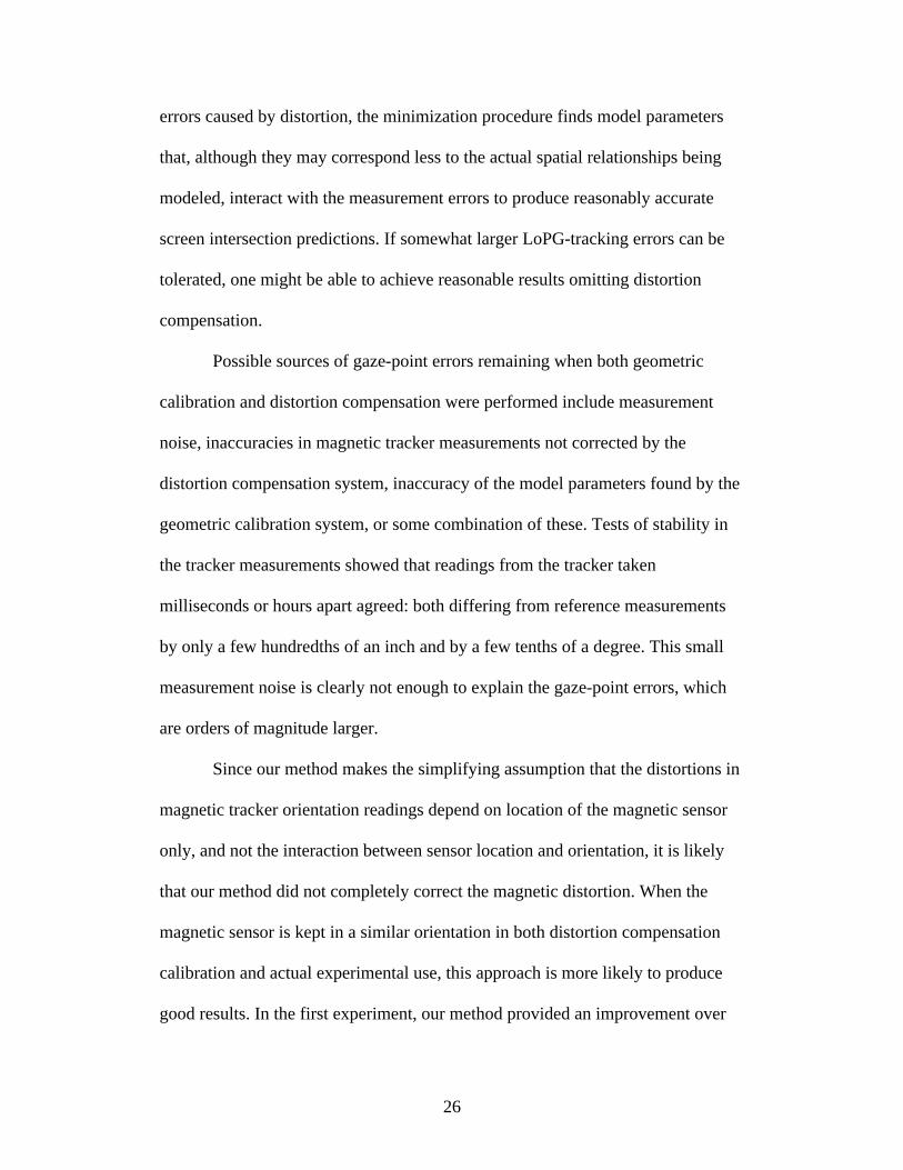
range of head movement needed for our walking simulator (Figure 1). This

simulator takes the form of a projected virtual environment where a subject views

computer generated images projected onto a large screen (Southard, 1995).

Access to the algorithms and intermediate variables computed within the

commercial gaze tracking systems is often not available. These may be useful for

combining gaze tracking with other experimental requirements, such as use of 3-

dimensional pointing devices or the tracking of multiple subjects.

A number of techniques exist for tracking eye movements (Young &

Sheena, 1975), but relatively little has been written on methods for combing

recordings of head and eye movements. A combined head and eye tracking

system was developed for use in a projected virtual environment (Asai, Osawa,

Takahashi, & Sugimoto, 2000), but few details of calibration methodology were

provided. Gaze tracking systems that combine head and eye movements have

been developed for head-mounted displays. Duchowski et al. (2002) describes a

virtual reality system based on a head-mounted display and incorporates a gaze

4

tracking system. Detailed descriptions of geometry and calibration techniques are

provided, but cannot be directly applied to projected virtual environments.

Towards developing a gaze tracking system for our walking simulator, we

separated the task into two parts: tracking the movement of the subject’s head and

tracking of rotation of the eye in its socket. Techniques for tracking the head are

useful for tasks where a subject “points” at objects by moving his or her head.

Such systems are in use in tactical aircraft: with the aid of a crosshair projected on

a helmet-mounted display, pilots can aim weaponry by turning their heads,

aligning the crosshair with a target (King, 1995).We developed a similar system

to allow subjects in our walking simulator to “point” at objects on a screen. By

equipping our subjects with a head-mounted sight (see Figure 2) and using a

magnetic head tracker and a tracking algorithm (described in the Method section),

we were able to find the point on the simulator’s screen that was aligned with a

mark at the center of the sight. For experiments, we align this mark to lie “straight

ahead” of the subject’s left eye. When the subject views a target through the

aligned mark, his or her eye is in the primary position of gaze as defined by Leigh

& Zee (1983). We use the term Line of Primary Gaze (LoPG) to describe the line

connecting the center of rotation of the subject’s left eye, and the center of the

pupil of that eye when the subject is looking straight ahead through the sight.

Experiments in our walking simulator require knowledge of the point of

intersection of LoPG with the screen within about two degrees.

A number of calibration challenges must be overcome for accurate

tracking of the LoPG. Our walking simulator uses a magnetic tracker (Blood,

5

1990) to measure location and orientation of the subject's head. These devices,

also used in biomechanics (Day, Dumas, & Murdoch, 1998), virtual reality

(Livingston & State, 1997) and eye-tracking research (Caldwell, Berbaum, &

Borah, 2000), are subject to environmental magnetic distortions that worsen with

distance between transmitter and sensor. Compensation for this distortion is

required if measurements are to be taken from near the limits of the tracker's

range or if the tracker is to be used near large metallic objects (Nixon, C., Fright,

& Price, 1998). Several methods for compensating for this distortion have been

proposed. A summary of several techniques was compiled by Kindratenko (2000).

Most of the techniques reviewed by Kindratenko were developed for virtual

reality, to allow for motion parallax as viewers move their heads, but are

applicable to gaze tracking. These distortion compensation techniques generally

require custom equipment and are not included in popular commercial gaze

tracking systems. For example, in a study investigating eye movements of

radiologists, Caldwell et al. (2000) used an ASL eye tracking system, but

employed a modified version of the ASL EYEPOS software and a custom

calibration fixture to correct for magnetic distortion. This method allowed for

more accurate gaze tracking near a metallic device, but few details of software

modifications were published.

In addition to compensating for magnetic distortion, the alignment

between the physical components of the tracking system must be found. The

distances between and relative orientations of these components become

parameters in the LoPG-tracking model. While direct measurement of these

6

parameters is possible, small errors in these measurements can lead to large errors

in computed LoPG. Developers of augmented reality systems (where visual

information is overlaid on an observer's view using a see-through head-mounted

display) have explored geometric models and calibration techniques like those

used in eye tracking. Calibration is required for aligning overlaid images with

real-world objects. Janin (1993) proposed calibrating the location of information

presented in a head-mounted display by aligning targets projected in the display

with markers on a real-world workbench in a series of intentional gazes. We used

a similar approach for LoPG calibration.

Our system allows for accurate (average error of less than two degrees)

tracking of LoPG over a wide range of head locations and orientations. This

system computes predicted gaze using a model of the geometry of gazes with few

simplifying assumptions. This allows model parameters for the gaze computation

algorithm to correspond to actual distances and angles between parts of the

tracking system, making direct verification possible. The general approach of this

algorithm can also be extended to incorporate additional or alternate sensors. The

addition of a head mounted eye tracker would allow for head-movement-

compensated gaze tracking.

<Figure 1 here>

7

METHOD

Apparatus

The LoPG tracking system we used to validate of our tracking algorithm

and calibration techniques was built on top of our walking simulator. It consisted

of the following:

Projection Screen: A 67 x 50 in. rear projection screen was used for

presentation of calibration targets. The bottom of the screen was elevated 30 in.

above the walking platform to place its center near eye-level for walking subjects.

Magnetic Tracker: An Ascension Flock-of-Birds magnetic tracker with

Extended Range Transmitter (Ascension Technology Corporation, Burlington,

VT) was used to monitor head position. This system reports location and

orientation of a small magnetic sensor in relation to a transmitter. The transmitter

was mounted on a 48 in. tall wood stand and was placed 52 in. to the right and 36

in. in front of the projection screen center.

Head-Mounted Sight: A head-mounted sight was used to allow subjects

to consistently direct their LoPG at projected screen targets. The sight was a 1/8

in. opaque mark on a clear plastic panel, which was in turn mounted on a 10 in.

lightweight brass boom extending from adjustable headgear. The magnetic tracker

sensor was attached to the headband as shown in Figure 2.

Computer: A Pentium computer running Microsoft Windows 2000,

Matlab 6.5 (The MathWorks Inc. Natick, MA), and custom software was used to

generate screen images of calibration targets, to control and record data from the

8

magnetic tracker and to perform calibration and gaze computations. Real-time

gaze computation software was written in C using Microsoft Visual Studio 6.0

and World Toolkit R9 (Sense8 Inc., San Rafael, CA). Calibration software was

written in Matlab.

<Figure 2 about here>

LoPG Tracking Algorithm

We developed an algorithm to transform raw position sensor readings into

experimental variables of interest for behavior research. The algorithm consists of

three steps: first, distortion compensation is performed—raw magnetic tracker

readings were corrected to compensate for the spatial distortions characteristic of

these devices. In this step, we attempted to compute the true location and

orientation of the magnetic sensor from its reported location. In the second step,

geometric transformation, corrected measurements, which describe the location

and orientation of the magnetic sensor in relation to the transmitter, were used to

find the LoPG relative to the projection screen. Thirdly, the LoPG can be used to

compute the point on the screen aligned with the aiming target. Here, we call this

on-screen location the “point of gaze.” The first and second steps of this algorithm

rely on parameters that are obtained through a pair of calibration processes

described below.

Distortion compensation. Examination of readings from our magnetic

tracker confirmed findings of other research (Bryson, 1992) that the distortion in

9

both the location and orientation components of the measurements varied

dramatically depending on location of the magnetic sensor. To account for these

distortions, we used a compensation function that added a correction factor to

measurements depending on the magnetic sensor location readings.

To compensate for distortion, the translational components (xo, yo, zo) of

each raw measurement from the magnetic tracker were processed with a

polynomial distortion correction function (Kindratenko, 1999). This correction

consisted of three polynomials in three variables of degree n. Each of these three

polynomials contained terms comprising the product of xo, yo and zo, raised to

powers in all combinations where the sum of the exponents was n or fewer:

∑∑∑= =

−

=

⋅⋅

+

=

n

i

i

j

ji

k

kjikj

ijk

ijk

ijk

o

o

o

c

c

c

zyxcba

zyx

zyx

0 0 0

--ooo (1)

where each aijk, bijk and cijk are t = (n+1)(n+2)(n+3)/6 polynomial coefficients, and

xC, yC and zC comprise the coordinates of the corrected measurement. Orientation

of the sensor, reported by the magnetic tracker as angles αo, βo and γo were

corrected using a similar set of polynomials:

∑∑∑= =

−

=

⋅⋅

+

=

n

i

i

j

ji

k

kjikj

ijk

ijk

ijk

o

o

o

c

c

c

zyxfed

0 0 0

--ooo

γβα

γβα

(2)

10

where dijk, eijk and fijk are each t polynomial coefficients, and αc, βc and γc are

corrected orientation angles. Correcting for distortion in this way assumes that the

distortion in orientation measurements depend only on location of the magnetic

sensor and not on orientation. Although distortion in orientation measurements

does indeed vary with sensor orientation (Livingston & State, 1997), this form of

distortion compensation is still effective if the sensor remains in the same relative

orientation in both calibration and experimental use. Polynomial coefficients in

Equations 1 and 2 correspond to the shape of the specific distortion in a given

experimental configuration and can be computed using the calibration procedure

described below. In agreement with the findings of Kindratenko (2000) we found

that a polynomial of degree n = 4 modeled the shape of the distortion well. A

fourth degree polynomial yielded t = 35 coefficients for each equation (210 in

total).

Geometric transformation. The second computational step of the LoPG

tracking algorithm transformed the distortion-compensated motion tracker

readings to locate LoPG in relation to the screen. This transformation employed a

geometric model of the spatial relationships between the eye and magnetic sensor

and of the relationship between the screen and the magnetic transmitter (Figure

3). The set of twelve model parameters computed in the geometric calibration

procedure described below characterizes these two relationships.

The model takes each of the following locations within the tracking

environment to be the origin of a three-dimensional coordinate frame: the upper

left corner of the screen (coordinate frame O), the measurement origin of the

11

magnetic transmitter (B), the measurement center of the magnetic sensor mounted

on the head (S) and the center of rotation of the eye (E). The x-, y- and z-axes of

each coordinate frame were oriented as shown in Figure 3.

<Figure 3 here>

We represented the spatial relationships between pairs of these coordinate

frames as 4x4 homogeneous transformation matrices. Each such matrix encodes

the relative locations and orientations of two coordinate frames and allows

locations measured in one frame to be transformed to the other. For each such

matrix,

=τ←

1000333231

232221

131211

abZ

Y

X

lrrrlrrrlrrr

(3)

representing the transformation from frame a to frame b, lX, lY and lZ are

equivalent to the three-dimensional location of the origin of a in the coordinate

system of b. The variables r are the lengths of the projections of unit vectors

along each of the three coordinate axes of frame a onto the axes of frame b. These

projections encode the rotational component of the transformation.

Since the LoPG lies along the x-axis of the eye frame E, to find LoPG

relative to the screen we find the location and orientation of this frame with

respect to the screen. To find this, we composed the matrix representations of the

spatial relationships measured by the magnetic tracker with matrices computed

12

through calibration. The position of the transmitter with respect to the screen

τO←B (transformation from transmitter frame to screen frame) and that of the eye

with respect to the sensor τS←E remain fixed for the duration of an experiment.

τB←S is constructed as follows from the 6 variables MC = (xc, yc, zc, αc, βc, γc)

resulting from the distortion compensation step above:

−

−

−

=τ←

1000100010001

10000)cos()sin(00)sin()cos(00001

10000)cos(0)sin(00100)sin(0)cos(

1000010000)cos()sin(00)sin()cos(

SB c

c

c

cc

cc

cc

cc

cc

cc

zyx

γγγγ

ββ

ββαααα

, (4)

where xc, yc and zc represent the corrected three dimensional distance between B

and S and αc, βc and γc are the corrected Euler angles describing the orientation of

S in the coordinate system of B.

Since composite transformations can be modeled as the product of

matrices, we can represent the location and orientation of the eye relative to the

screen as follows:

ττττ←←←←

=ESSBBOEO

. (5)

13

Once τO←E has been computed, we can easily find both the eye location with

respect to the screen1 (simply the last column of τO←E) and the screen intersection

of the LoPG.

Point of gaze computation. The point on the screen that intersects the

subject’s LoPG can be found from τO←E, the result of the geometric

transformation portion of the gaze-tracking algorithm. In our model, the LoPG

falls along the x-axis of the eye coordinate frame. We solve for a point that is on

the x-axis of the eye frame, which also falls in the x-y plane of the screen

coordinate frame – the surface of the screen. This can be formulated as a linear

system consisting of a point on the x-axis of frame E, at (xi, 0, 0), transformed by

τO←E and set equal to a point in the x-y plane of frame O, (Ix, Iy, 0).

=

⋅τ←

10

100

EO

y

xi

IIx

(6)

Solving this system for Ix and Iy gives us the intersection between the LoPG and

the plane of the screen, expressed in the screen coordinate frame.

Calibration

14

Parameters used in the LoPG tracking algorithm were computed via two

calibration steps. First, the distortion in magnetic tracker readings was measured

and coefficients for the compensation polynomials (Equations 1 and 2) were

computed. This process was carried out when the tracking system was installed.

Computed coefficients can be reused, assuming no changes to the relative

placement of the tracker transmitter and distortion-causing (large metal) objects.

The second calibration step computes both the spatial relationship between the

magnetic tracker sensor and the eye and the relationship between the tracker

transmitter and the screen image. This step is performed once for each subject

before an experimental run, as adjustment of the motion tracker headband or

image projected on the screen alters the spatial relationships measured in this

calibration.

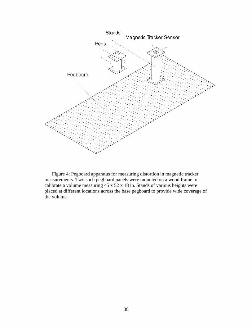
Distortion compensation calibration. To compute coefficients of the

distortion compensation polynomials (Equations 1 and 2), we compared a set of

tracker readings taken over a grid of known points within the tracking volume to

the hand-measured locations of those points. The differences between the

measured and reported locations form a set of vectors mapping points in reported

space to actual physical locations. These error vectors were usually small near the

transmitter and became large (in our case, up to 13 in.) near the outer third of the

nominal volume of the tracker's range. The method then involved solving for the

set of polynomial coefficients that, when used in Equations 1 and 2, minimized

the sum of the squared lengths of these error vectors.

15

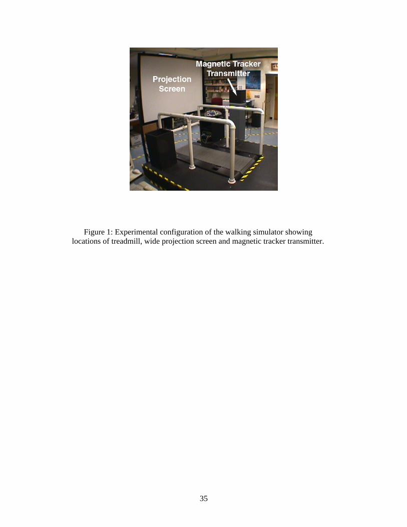
In our walking simulator environment, we constructed a system of

pegboards and stands to provide a set of known locations for placement of the

motion tracker during this procedure. The pegboard system, shown in Figure 4,

was constructed from 24 x 48 in. sheets of predrilled 1/4 in. thick pegboard

mounted on a wood frame. Screws used in the construction of the frame were

replaced with glue after we found them to be causing small local distortions in

magnetic tracker readings. The sensor stands were constructed from sections of 4

in. diameter PVC pipe with flat pegboard caps on each end. Each stand held the

magnetic tracker sensor rigidly on one end cap and had pegs for attachment to the

pegboard on the other. The sensor was positioned so that when the stands were

engaged with the pegboard, the sensor's x-axis (see Figure 3) pointed towards the

screen and its z-axis pointed towards the floor. In this orientation, the magnetic

tracker reported azimuth, elevation and roll of the sensor to all be near zero

(where distortions in orientation measurements were small). Several pipe lengths

were used for measurements at varying heights (0, 6, 12 and 18 in.) above the

pegboard plane. Other systems for placing a sensor at known location have also

been developed, including a fixture made entirely of Plexiglas (Caldwell et al.,

2000) and an optical tracking system (Ikits, Brederson, Hansen, & Hollerbach,

2001).

<Figure 4 here>

16

The pegboard frame was placed in our tracking environment and squared with the

case of the magnetic tracker transmitter. The location of the pegboard grid with

respect to the magnetic transmitter was then measured.2 Readings from the

motion tracker were taken over both a sparse three-dimensional grid of 64

locations spanning 45 x 52 x 18 in. (see Figure 5) and a more dense, smaller grid

of 128 locations covering the central 32 x 40 x 18 in. of the same space. The

magnetic tracker readings from both grids were combined to form the dataset of

reported locations and orientations. Using Matlab, we performed a linear least-

squares fit on the differences between reported and pegboard-measured data sets

to find the coefficients for the distortion correction polynomials. An illustration of

the magnitude of location distortion is provided in Figure 5.

<Figure 5 here>

Geometric calibration. The second calibration step computed the

geometric model parameters describing spatial relationships τO←B and τS←E.

These parameters, corresponding to the alignment of the screen with the tracker

transmitter (τO←B) and position of the magnetic tracker sensor relative to the eye

(τS←E), are difficult to measure directly and τS←E changes from subject to subject

or whenever the headband is adjusted. For these reasons, we developed a

calibration procedure to quickly ascertain these model parameters.

17

Geometric calibration of the gaze-tracking system was performed by

taking magnetic tracker recordings while subjects performed a series of

constrained gazes. For each gaze the subject, using his left eye, aligned the head-

mounted sight with a target dot projected on the screen. The subject repeated this

procedure from a series of standing locations within the desired usage space.

After a number of such gazes, a pair of τO←B and τS←E parameters is computed

by the Gauss-Newton non-linear least squares fitting method as described in the

next section.

Geometric calibration algorithm. The fitting procedure sought the set of

model parameters that, when combined with the geometric model in our LoPG-

tracking algorithm, best predicted onscreen points of gaze from distortion-

compensated magnetic tracker readings (as computed in step 1) over a set of

directed gazes. Generally, for a model F, the model-predicted outcome W can be

represented as

W = F(P,M) (7)

where

P = [p1, p2, p3, … pq] (8)

are the model parameters (a total of q) and

18

M = [m1, m2, m3, … mr] (9)

are the inputs to the model (a total of r). The outcome predicted by our model, Wc

(the two-dimensional screen location of predicted gaze), is expressed as

Wc = Fc(PC,MC), (10)

where Fc is the function that computes point of gaze from a given magnetic

tracker reading and a set of model parameters (Equations 5 and 6). PC is the set of

twelve model parameters representing the spatial relationships τO←B and τS←E

(the twelve parameters describe, for each of the two transformations, a three-

dimensional distance between coordinate frames and three Euler angles

describing relative orientations of the coordinate frames), and MC is the magnetic

tracker measurement (three distances and three angles) corrected for distortion by

Equations 1 and 2. We determined quality of the fit found by the geometric

calibration procedure by the size of the average error across all gazes in a

calibration. This “mean gaze-point error” was expressed as the sum across all

calibration gazes of the distances along the screen between the actual calibration

targets and the predicted points of gaze. The fitting procedure sought to find a set

of model parameters, PC, to minimize this sum, given a set of magnetic tracker

measurements, MC and a “guess” of PC. Starting at the given guess of PC, the

fitting procedure iteratively adjusted these parameters until a local minimum in

mean gaze-point error was found3. Minimization was performed in Matlab using

19

the nlinfit function (from the statistics toolbox; an implementation of the Gauss-

Newton fitting method). In our implementation, this technique found a Pc

corresponding to a given Wc and Mc for twenty calibration gazes in about 10

seconds.

Experimental Validation

To test the calibration and LoPG-tracking techniques presented in this

paper, we first calibrated the distortion compensation system as described above

and then performed two target-sighting experiments. In the first experiment, we

performed the geometric calibration procedure using the beam of a laser pointer to

represent the line of gaze of the human subject. This allowed the simulated Line

of Primary Gaze to be precisely aligned with calibration targets projected on the

screen and allowed testing without the variability of human subjects’ ability to

maintain head position. To fix the relative placement of the laser and sensor, both

were attached to a small wooden block. The sensor was placed on the block with

its x-axis approximately parallel to and two inches above the laser beam. This

alignment enabled us to easily measure the actual spatial relationship between the

sensor and the laser for validation of the parameters found by the geometric

calibration procedure. (We found it much more difficult to measure the equivalent

relationship, τS←E, on a human subject.) The wood block holding the sensor and

laser was fastened to a tripod and raised to a height approximating that of a

human subject’s head. To gather data for testing the geometric calibration

procedure, the tripod was placed at 10 locations. These locations were chosen

20

within the range of possible standing positions of our research subjects (an area

about 36 x 36 in.). For each of the 10 tripod locations, readings from the magnetic

tracker were taken, panning and tilting the tripod head so that the laser beam fell

on each calibration target. Four of the targets were just inside the corners of the

screen, one was placed in the center and five other locations were arbitrarily

chosen. The targets remained in the same locations throughout each experiment.

Due to the distance between the sensor and the pivot point of the tripod head, for

a given tripod location the actual sensor locations varied by up to 8 in. as the head

was tilted at different angles to align the laser.

In a second experiment, a similar set of 100 directed gazes was performed

by a human subject. The subject used the head-mounted sight (Figure 2) to align

his LoPG with each of the 10 targets from each of 10 standing locations. The five

of the calibration targets that were arbitrarily placed in the first experiment were

in somewhat different locations for calibration of the human subject.

Data from both procedures were independently used to calibrate the

LoPG-tracking system and the benefit of distortion compensation and geometric

calibration procedures were examined.

RESULTS

For each of the two experiments, collected data consisted of a set of 100

six-variable tracker readings (each taken when the laser/LoPG was aligned to fall

at the center of a calibration target) and the 100 two-dimensional screen locations

of the corresponding calibration targets. Location and orientation data from the

21

magnetic tracker were passed through the distortion compensation functions

(Equations 1 and 2) yielding a second set of 100 corrected tracker readings for

each experiment. We independently used subsets of this body of distortion-

corrected data to derive the transformation matrices τO←B and τS←E using the

geometric calibration procedure described above and tested these fits against the

remaining data. We compared point of gaze computations made with and without

distortion compensation or geometric calibration to known target locations. By

varying the size of the subsets of the collected dataset used to compute τO←B and

τS←E, we also found the number of calibration points needed to adequately

decrease mean angular error across all computed gaze lines to the desired two

degrees.

Accuracy of predicted point of gaze. Using the distortion-corrected

location and orientation measurements from the entire set of 100 laser-target

alignments from the first experiment and the geometric calibration procedure, the

matrices τO←B and τS←E were computed. Equations 5 and 6 were then used to

predict point of gaze for each of the 100 laser-target alignments and mean gaze-

point error (mean distance along the screen between calibration target and point of

gaze predicted by LoPG-tracking algorithm) was computed. For the dataset from

the first experiment, mean error was 1.46 in. Error can also be described as the

angle between the screen target and computed point of gaze when viewed from

22

the location of the magnetic sensor. Measured in this way, mean angular error was

1.52 degrees.

To examine the effect of distortion compensation on gaze-point error, we

also performed the geometric calibration procedure using raw magnetic tracker

measurements not processed by the distortion correction polynomials. As seen in

Figure 6B, without distortion compensation, mean gaze-point error was

significantly larger (paired t-test, T99 = -4.52, p < 0.001) at 1.93 in. when

calibrating using the same dataset (an increase of 32%). Without distortion

compensation, clear outliers from the clusters of points of gazes can be seen for

most of the screen targets in Figure 6B. These outlying points of gaze were all

from the tripod location most distant from the magnetic transmitter, where

distortion was largest. Distortion compensation provided most benefit for this

tripod location (Figure 9).

To examine the effect of the geometric calibration procedure on accuracy

of predicted LoPG, we also computed mean gaze-point error across the collected

dataset using only a hand-measured estimate of τO←B and τS←E: no geometric

calibration was performed. As one might expect, without calibration, errors were

significantly larger (paired t-test, T99 = -12.2, p < 0.001). Mean gaze-point error

using an uncalibrated model was 4.07 in., as seen in Figure 6C.

We also examined the ability of the geometric model to compute points of

gaze both without distortion compensation and without geometric calibration. The

23

hand-measured τO←B and τS←E and raw magnetic tracker readings were used in

Equations 5 and 6. Mean gaze-point error was 5.66 in.

Conducting the same analysis for the data from the second experiment, we

found mean gaze-point error to be lower than that in the first experiment when

geometric calibration was performed. When both distortion compensation and

geometric calibration were used, mean error was 0.80 in. When geometric

calibration was performed on data not corrected for distortion, mean error was

1.10 in. Without geometric calibration, error was much larger, as we were unable

to measure τS←E with the same accuracy for the second experiment. With and

without distortion correction, mean errors were 39.7 and 42.6 in. respectively.

Reasons for the reduced errors in the second experiment are proposed in the

Discussion section.

<Figure 6 here>

Short calibration. It is important to be able to find geometric model

parameters from a small number of calibration points. In order to use our LoPG

tracking system as a tool for gathering data from untrained research subjects, we

must calibrate the system using only as few data points as necessary. To find the

number of calibration data points needed to accurately predict point of gaze, we

created calibration sets from subsets of the 100 measurements collected in the first

experiment. We used these small calibration sets to compute τO←B and τS←E and

then used those computed parameters to calculate screen intersections across the

full set of 100 measurements. Comparing the calculated and actual screen

24

intersections, we examined the quality of the parameters. We performed this

technique for calibration sets of varying sizes, across 100 random orderings of the

100 data points collected in the first experiment. We found that after about 20

points, the geometric calibration system converges to a point of gaze with an

average error of less than 2 in., with only small improvements attained by

including additional points in the calibration set (Figure 7).

We also performed the same procedure on the dataset generated in

experiment 2 (by the human subject). As overall gaze-point error was lower when

calibration was performed with the entire dataset, the desired 2 in. of error could

be reached with about 10 data points (Figure 8). Calibrations performed with

more than 15 data points provided only a small additional benefit.

In the processing of calibration data in sets of differing sizes, geometric

calibration occasionally failed completely, producing larger mean gaze-point error

than if geometric calibration had not been performed at all. These failures were

common with very small calibration sets, but never occurred with sets of 10

points or more. In all cases where calibration failed, the addition of one or two

calibration points to the set was enough to reverse the failure (Figure 8).

<Figures 7,8 here>

Effect of sensor location on error. Using the raw data (not compensated

for distortion) from the first experiment and computing point of gaze without

performing geometric calibration, the farther the sensor was from the transmitter

the worse the error (Pearson correlation, r = 0.53, n = 100, p < 0.001) and that

error was manifest as an increasing error in the y-dimension (Pearson correlation,

25

r = 0.56, n = 100, p < 0.001). When both the distortion correction and the

geometric calibration were implemented, the errors were more evenly distributed

(Figure 9), resulting in no significant correlation with distance from the

transmitter (Pearson correlation, r = 0.08, n = 100, p < 0.43). There was, however,

a significant tendency for the errors to increase towards the screen (i.e. in the x

dimension; Pearson correlation, r = 0.27, n = 100, p = 0.007).

<Figure 9 here>

DISCUSSION

The LoPG tracking model and calibration techniques presented here

succeed at accurately predicting the on-screen location of gaze while subjects

look through a head-mounted sight. The validation experiments show that, in

agreement with Caldwell et al. (2000), the use of polynomial distortion

compensation can improve the accuracy of gaze-point calculations (Figure 6C,

D). In addition, benefit was also seen from geometric calibration. The model

presented for tracking LoPG provides a foundation for future gaze-tracking

systems.

An interesting result of performing calibration both with and without

distortion compensation was that while point of gaze was predicted more

accurately with distortion compensation, the tracking system still performed

relatively well in the presence of uncompensated distortion provided that

geometric calibration was performed (Figure 6B). In the presence of measurement

26

errors caused by distortion, the minimization procedure finds model parameters

that, although they may correspond less to the actual spatial relationships being

modeled, interact with the measurement errors to produce reasonably accurate

screen intersection predictions. If somewhat larger LoPG-tracking errors can be

tolerated, one might be able to achieve reasonable results omitting distortion

compensation.

Possible sources of gaze-point errors remaining when both geometric

calibration and distortion compensation were performed include measurement

noise, inaccuracies in magnetic tracker measurements not corrected by the

distortion compensation system, inaccuracy of the model parameters found by the

geometric calibration system, or some combination of these. Tests of stability in

the tracker measurements showed that readings from the tracker taken

milliseconds or hours apart agreed: both differing from reference measurements

by only a few hundredths of an inch and by a few tenths of a degree. This small

measurement noise is clearly not enough to explain the gaze-point errors, which

are orders of magnitude larger.

Since our method makes the simplifying assumption that the distortions in

magnetic tracker orientation readings depend on location of the magnetic sensor

only, and not the interaction between sensor location and orientation, it is likely

that our method did not completely correct the magnetic distortion. When the

magnetic sensor is kept in a similar orientation in both distortion compensation

calibration and actual experimental use, this approach is more likely to produce

good results. In the first experiment, our method provided an improvement over

27

omitting orientation distortion compensation entirely as sensor alignment was

similar in calibration and experiment, but it is likely that distortion still plays a

role in gaze-point errors. In the second experiment, we found even lower mean

gaze-point error when magnetic tracker measurements were corrected for location

distortion, but not orientation distortion. As the magnetic tracker is rotated on its

side when attached to the headgear of the head-mounted sight (Figure 2), it is no

longer in the relative orientation needed to see a benefit from our compensation

for orientation distortion. Expanding the distortion compensation calibration

procedure to measure the sensor at multiple orientations for each grid location

sampled could further reduce error due to distortion. This would however

multiply the number of data points collected – and the time required to perform of

the data collection procedure – by the number of orientations to be sampled.

The geometric calibration algorithm seeks a τO←B and τS←E yielding a

local minimum in gaze-point error, starting from the initial guess derived from

hand-measurements of these parameters. Control experiments were performed to

verify that no other, potentially lower, minima could be found near the minima

arrived at by calibration. Initial guesses were perturbed by several inches in all

directions, but the calibration system still converged on parameters predicting the

same LoPG. This implies that uncorrected distortion in magnetic tracker

measurements is still the leading cause of gaze-point error.

Comparison between points of gaze computed with (Figure 6C) and

without (Figure 6C) the geometric calibration step, shows that attempts to directly

measure the spatial relationships τO←B and τS←E (i.e. without) leads to relatively

28

large gaze-point errors. Application of the geometric fitting procedure

substantially improves the ability of the model to find LoPG. Although it is not

surprising that better results can be obtained when calibration is performed, it is

interesting to note that the parameters resulting from calibration deviated

considerably from hand-measured parameters. In fact, the optimized parameters

comprising τS←E indicated spatial relationships that were clearly inconsistent with

the actual configuration of the laser and magnetic sensor. For example,

parameters producing the least mean gaze-point error contained values for the

distance between the magnetic sensor and the LoPG that were several inches

greater than physical measurements indicated. Although there is some imprecision

(we estimate about a quarter of an inch) in measuring straight-line distance

between eye and magnetic sensor, this imprecision alone cannot explain the

difference. Since calibration performed with data from the human subject seemed

less prone to this inconsistency, we suspect that the constraints imposed on the

movement of the laser and sensor by the tripod head may be responsible. In

positioning the laser to align it with calibration targets, the sensor remained within

47 degrees of level and “roll” of the sensor could not be performed. These

constraints lead to less variation in the calibration data and in turn may have

under-constrained the fitting procedure used in geometric calibration.

A limitation of the geometric calibration procedure described here is the

inability of the calibration procedure to locate the eye along the LoPG. Although

this limitation does not impact the ability of the system to predict points of gaze

on the screen, it does impact the veracity of the model parameters. Although the

29

geometric model used specifies the eye as a coordinate frame, with an origin

located some distance from the magnetic tracker sensor, the geometric calibration

procedure constrains only the x-axis of this coordinate frame. This leads to an

infinite number of possible sets of model parameters that still predict the same

point of gaze on the screen (i.e. screen intersection remains the same even if the

eye were to slide forward or back along the LoPG, or rotate on its x-axis). This

means that the parameters comprising τS←E found by the fitting procedure

correspond to one possible location of the eye along the LoPG. Control

experiments showed that the fitted location along the line on of the LoPG

depended on the initial guess used for the fitting procedure. If the intermediate

results of the model are to be used, for example for computing the location of the

eye relative to the screen for placement of a camera in a virtual environment, the

inability of this system to precisely locate the eye might be overcome by

performing an additional calibration. Alternately, a calibration similar to the one

used in this paper, but requiring the subject to place the eye in other, non-primary

positions of gaze could be used to find actual eye location. This technique is

currently being investigated.

30

REFERENCES

Asai, K., Osawa, N., Takahashi, H., & Sugimoto, Y. Y. (2000). Eye Mark Pointer

in Immersive Projection Display. Paper presented at the IEEE Virtual

Reality 2000 Conference, New Brunswick, New Jersey.

Blood, E. (1990).U.S. Patent No. 4,945,305. Washington, DC: U.S. Patent and

Trademark Office.

Bryson, S. (1992). Measurement and calibration of static distortion of position

data from 3D trackers. Paper presented at the SPIE Stereoscopic displays

& applications III, San Jose.

Caldwell, R. T., Berbaum, K. S., & Borah, J. (2000). Correcting errors in eye-

position data arising from the distortion of magnetic fields by display

devices. Behavior Research Methods, Instruments, & Computers, 32(4),

572-578.

Day, J. S., Dumas, G. A., & Murdoch, D. J. (1998). Evaluation of a long-range

transmitter for use with a magnetic tracking device in motion analysis.

Journal of Biomechanics, 31(10), 957-961.

Duchowski, A., Medlin, E., Cournia, N., Murphy, H., Gramopadhye, A., Nair, S.,

et al. (2002). 3-D eye movement analysis. Behavior Research Methods,

Instruments, & Computers, 34(4), 573-591.

Ikits, M., Brederson, J. D., Hansen, C. D., & Hollerbach, J. M. (2001). An

improved calibration framework for electromagnetic tracking devices.

Paper presented at the Virtual Reality, 2001. Proceedings. IEEE.

31

Janin, A., Mizell, D., & Caudell, T. (1993). Calibration of head-mounted displays

for augmented reality applications. Paper presented at the Virtual Reality

Annual International Symposium.

Kindratenko, V. V. (1999). Calibration of electromagnetic tracking devices.

Virtual Reality: Research, Development, & Applications, 4, 139-150.

Kindratenko, V. V. (2000). A survey of electromagnetic position tracker

calibration techniques. Virtual Reality: Research, Development, &

Applications, 5(3), 169-182.

King, P. (1995). Integration of helmet-mounted displays into tactical aircraft.

Proceedings of the Society for Information Display, XXVI, 663-668.

Leigh, R. J., & Zee, D. S. (1983). The Neurology of Eye Movements. Philadelphia:

F. A. Davis Company.

Livingston, M. A., & State, A. (1997). Magnetic Tracker Calibration for

Improved Augmented Reality Registration. Presence: Teleoperators &

Virtual Environments, 6(5), 532-546.

Nixon, M., C., M. B., Fright, R. W., & Price, B. N. (1998). The Effects of Metals

and Interfering Fields on Electromagnetic Trackers. Presence, 7(2), 204-

218.

Southard, D. A. (1995). Viewing Model for virtual environment displays. Jorunal

of Electronic Imaging, 4(4), 413-420.

Young, L. R., & Sheena, D. (1975). Survey of eye movement recording methods.

Behavior Research Methods, Instruments, & Computers, 7(5), 397-429.

32

FIGURE CAPTIONS

Figure 1: Experimental configuration of the walking simulator showing

locations of treadmill, wide projection screen and magnetic tracker transmitter.

Figure 2: Head-mounted sight. Subject aligned objects of interest with a

sighting mark. When viewing objects through the mark, the left eye is held in

primary position of gaze.

Figure 3: Geometric model for finding Line of Primary Gaze (LoPG) by

combining the spatial relationship measured by the magnetic tracker with those

derived through geometric calibration.

Figure 4: Pegboard apparatus for measuring distortion in magnetic tracker

measurements. Two such pegboard panels were mounted on a wood frame to

calibrate a volume measuring 45 x 52 x 18 in. Stands of various heights were

placed at different locations across the base pegboard to provide wide coverage of

the volume.

Figure 5: Distortion measured in performing distortion compensation

calibration of magnetic tracker. Axis units are inches in the coordinate system of

the magnetic tracker transmitter. Shade of surface indicates magnitude of

distortion in location portion of magnetic tracker measurements. Darkest areas

indicate distortion in location measurement of over 13 inches.

Figure 6: Effects of distortion compensation (C, D) and geometric calibration

(B, D) on computation of points of gaze. Data were collected with a laser pointer

used to simulate Line of Primary Gaze (LoPG). Circular marks indicate screen

33

location of calibration targets. Crosses are laser-screen intersections (“points of

gaze”) computed by LoPG-tracking algorithm. Within each cluster, each cross

represents a measurement from a different tripod location. Rectangular outline

shows location of screen. Screen outline and targets appear at hand measured

location (A, C) and location found by geometric calibration (B, D).

Figure 7: Error in computed point of gaze derived when model was calibrated

with increasing numbers of calibration points, across 100 random orderings of the

data set collected in the first experiment. Mean gaze-point error is reduced to

within 2 inches after twenty directed gazes. *The result of one calibration, where

the algorithm did not converge and very large (1034 in.) average error resulted,

was removed for this plot.

Figure 8: Error in computed point of gaze derived when model was calibrated

with increasing numbers of calibration points, across 100 random orderings of the

data set collected in the second experiment. Mean gaze-point error was reduced to

less than two degrees in only 10 directed gazes. Dark line shows an example

calibration where the fitting procedure failed to converge.

Figure 9: The mean gaze-point error at each of the 10 tripod locations, on the

left using the raw data from the position sensor collected in the first experiment

(see Figure 6D) and on the right using the same data corrected using both the

distortion compensation and the geometric calibration. The tripod was on the

treadmill and the laser pointer, to which the sensor was attached, was directed

towards the screen, which is shown as the long white rectangle on the right of

each panel. The transmitter is shown as the black square. Each circle represents

34

one of the tripod locations, with radius equal to the mean gaze-point error from

that location. Mean gaze-point error for each location also shown in the center of

the corresponding circle.

35

Figure 1: Experimental configuration of the walking simulator showing locations of treadmill, wide projection screen and magnetic tracker transmitter.

36

Figure 2: Head-mounted sight. Subject aligned objects of interest with a sighting mark. When viewing objects through the mark, the left eye is held in primary position of gaze.

37

Figure 3: Geometric model for finding Line of Primary Gaze (LoPG) by

combining the spatial relationship measured by the magnetic tracker with those derived through geometric calibration.

38

Figure 4: Pegboard apparatus for measuring distortion in magnetic tracker measurements. Two such pegboard panels were mounted on a wood frame to calibrate a volume measuring 45 x 52 x 18 in. Stands of various heights were placed at different locations across the base pegboard to provide wide coverage of the volume.

39

Figure 5: Distortion measured in performing distortion compensation calibration of magnetic tracker. Axis units are inches in the coordinate system of the magnetic tracker transmitter. Shade of surface indicates magnitude of distortion in location portion of magnetic tracker measurements. Darkest areas indicate distortion in location measurement of over 13 inches.

40

Figure 6: Effects of distortion compensation (C, D) and geometric calibration (B, D) on computation of points of gaze. Data were collected with a laser pointer used to simulate Line of Primary Gaze (LoPG). Circular marks indicate screen location of calibration targets. Crosses are laser-screen intersections (“points of gaze”) computed by LoPG-tracking algorithm. Within each cluster, each cross represents a measurement from a different tripod location. Rectangular outline shows location of screen. Screen outline and targets appear at hand measured location (A, C) and location found by geometric calibration (B, D).

41

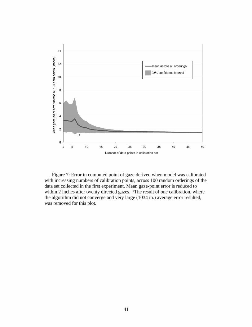
Figure 7: Error in computed point of gaze derived when model was calibrated with increasing numbers of calibration points, across 100 random orderings of the data set collected in the first experiment. Mean gaze-point error is reduced to within 2 inches after twenty directed gazes. *The result of one calibration, where the algorithm did not converge and very large (1034 in.) average error resulted, was removed for this plot.

42

Figure 8: Error in computed point of gaze derived when model was calibrated with increasing numbers of calibration points, across 100 random orderings of the data set collected in the second experiment. Mean gaze-point error was reduced to less than two degrees in only 10 directed gazes. Dark line shows an example calibration where the fitting procedure failed to converge.

43

Figure 9: The mean gaze-point error at each of the 10 tripod locations, on the left using the raw data from the position sensor collected in the first experiment (see Figure 6D) and on the right using the same data corrected using both the distortion compensation and the geometric calibration. The tripod was on the treadmill and the laser pointer, to which the sensor was attached, was directed towards the screen, which is shown as the long white rectangle on the right of each panel. The transmitter is shown as the black square. Each circle represents one of the tripod locations, with radius equal to the mean gaze-point error from that location. Mean gaze-point error for each location also shown in the center of the corresponding circle.

44

NOTES

1 This position is used in projected virtual reality displays to determine how to position the virtual

camera when generating an image of a scene.

2 Even if the tracker is not aligned exactly with the case of the transmitter, the correction

polynomials (Equations 1 and 2) we computed include terms to account for such an offset: These

offsets are contained in the constant (i = 0) and linear (i = 1) terms of polynomials.

3 It should be noted that the calibration procedure described here does not completely constrain the

model parameters used. As no measurement of orientation on the screen of the center of gaze, or

distance from eye to screen during a fixation is made, neither of these can be predicted by the

model. As a result, the best fit model parameters describing τS←E may converge on any one of a

line of solutions corresponding to possible locations of the eye along the LoPG. Each of these eye

locations predicts the same LoPG location on the screen.