TRACKING IN WIRELESS SENSOR NETWORK USING BLIND …

TRACKING IN WIRELESS SENSOR NETWORK USING

BLIND SOURCE SEPARATION ALGORITHMS

ANIL BABU VIKRAM

Bachelor of Technology (B.Tech)

Electronics and Communication Engineering(E.C.E)

Jawaharlal Nehru Technological University,India

May, 2006

submitted in partial fulfillment of the requirements for the degree

MASTER OF SCIENCE IN ELECTRICAL ENGINEERING

at the

CLEVELAND STATE UNIVERSITY

NOVEMBER, 2009

This thesis has been approved for the

Department of ELECTRICAL AND COMPUTER ENGINEERING

and the College of Graduate Studies by

Thesis Committee Chairperson, Dr. Ye Zhu

Department/Date

Dr. Vijay K. Konangi

Department/Date

Dr. Yongjian Fu

Department/Date

To my Parents and Friends

ACKNOWLEDGMENTS

I would like to thank my advisor Dr.Ye Zhu, for constant support, motivation

and guidance.

I would like thank committee members Dr. Vijay K. Konangi, Dr. Yongjian

Fu for their support. I am very appreciate for Dr. Zhu giving me an opportunity to

work in Network Security and Privacy research group.

I would like to thank my research group members for their support and friend-

ship.

Special thanks and appreciation go to my family and friends for their moral

and physical support. Special thanks to my sister Sakuntala and a good friend Srikar

for constant moral support.

iv

TRACKING IN WIRELESS SENSOR NETWORK USINGBLIND SOURCE SEPARATION ALGORITHMS

ANIL BABU VIKRAM

ABSTRACT

This thesis describes an approach to track multiple targets using wireless sen-

sor networks. In most of previously proposed approaches, tracking algorithms have

access to the signal from individual target for tracking by assuming (a) there is only

one target in a field, (b) signals from different targets can be differentiated, or (c)

interference caused by signals from other targets is negligible because of attenuation.

We propose a general tracking approach based on blind source separation, a statistical

signal processing technique widely used to recover individual signals from mixtures

of signals. By applying blind source separation algorithms to mixture signals col-

lected from sensors, signals from individual targets can be recovered. By correlating

individual signals recovered from different sensors, the proposed approach can esti-

mate paths taken by multiple targets. Our approach fully utilizes both temporal

information and spatial information available for tracking. We evaluate the proposed

approach through extensive experiments. Experiment results show that the proposed

approach can track multiple objects both accurately and precisely. We also propose

cluster topologies to improve tracking performance in low-density sensor networks.

Parameter selection guidelines for the proposed topologies are given in this Thesis.

We evaluate proposed cluster topologies with extensive experiments. Our empirical

experiments also show that BSS-based tracking algorithm can achieve comparable

tracking performance in comparison with algorithms assuming access to individual

signals.

v

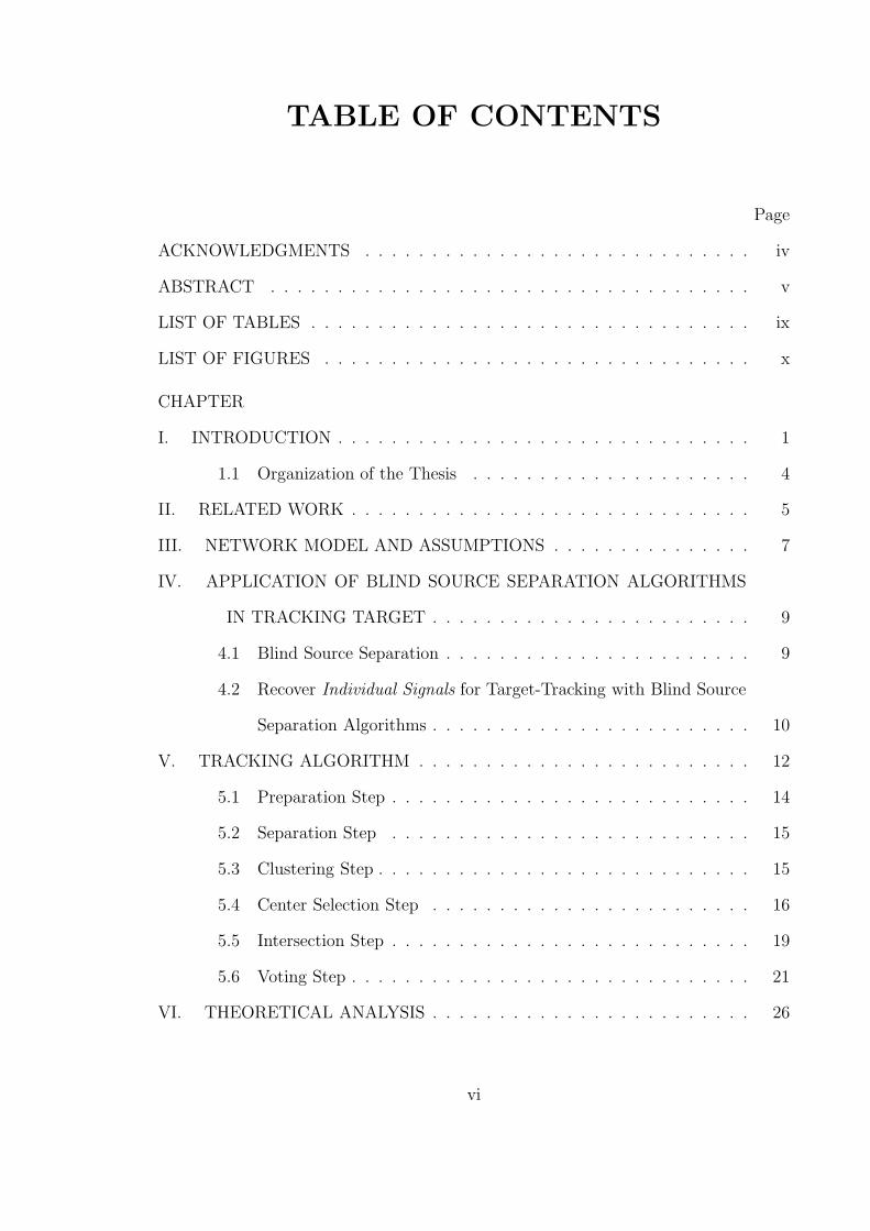
TABLE OF CONTENTS

Page

ACKNOWLEDGMENTS . . . . . . . . . . . . . . . . . . . . . . . . . . . . . iv

ABSTRACT . . . . . . . . . . . . . . . . . . . . . . . . . . . . . . . . . . . . v

LIST OF TABLES . . . . . . . . . . . . . . . . . . . . . . . . . . . . . . . . . ix

LIST OF FIGURES . . . . . . . . . . . . . . . . . . . . . . . . . . . . . . . . x

CHAPTER

I. INTRODUCTION . . . . . . . . . . . . . . . . . . . . . . . . . . . . . . . 1

1.1 Organization of the Thesis . . . . . . . . . . . . . . . . . . . . . 4

II. RELATED WORK . . . . . . . . . . . . . . . . . . . . . . . . . . . . . . 5

III. NETWORK MODEL AND ASSUMPTIONS . . . . . . . . . . . . . . . 7

IV. APPLICATION OF BLIND SOURCE SEPARATION ALGORITHMS

IN TRACKING TARGET . . . . . . . . . . . . . . . . . . . . . . . . 9

4.1 Blind Source Separation . . . . . . . . . . . . . . . . . . . . . . . 9

4.2 Recover Individual Signals for Target-Tracking with Blind Source

Separation Algorithms . . . . . . . . . . . . . . . . . . . . . . . . 10

V. TRACKING ALGORITHM . . . . . . . . . . . . . . . . . . . . . . . . . 12

5.1 Preparation Step . . . . . . . . . . . . . . . . . . . . . . . . . . . 14

5.2 Separation Step . . . . . . . . . . . . . . . . . . . . . . . . . . . 15

5.3 Clustering Step . . . . . . . . . . . . . . . . . . . . . . . . . . . . 15

5.4 Center Selection Step . . . . . . . . . . . . . . . . . . . . . . . . 16

5.5 Intersection Step . . . . . . . . . . . . . . . . . . . . . . . . . . . 19

5.6 Voting Step . . . . . . . . . . . . . . . . . . . . . . . . . . . . . . 21

VI. THEORETICAL ANALYSIS . . . . . . . . . . . . . . . . . . . . . . . . 26

vi

6.1 Signal Attenuation . . . . . . . . . . . . . . . . . . . . . . . . . . 26

6.2 Tracking Resolution . . . . . . . . . . . . . . . . . . . . . . . . . 28

6.2.1 Finest Tracking Resolution . . . . . . . . . . . . . . . . . 30

6.2.2 Average Tracking Resolution . . . . . . . . . . . . . . . . 31

6.3 Effect of Moving Speed . . . . . . . . . . . . . . . . . . . . . . . 31

VII. EMPIRICAL EVALUATION . . . . . . . . . . . . . . . . . . . . . . . 33

VIII. PERFORMANCE EVALUATION . . . . . . . . . . . . . . . . . . . . 35

8.1 Experiment Setup . . . . . . . . . . . . . . . . . . . . . . . . . . 35

8.2 Performance Metrics . . . . . . . . . . . . . . . . . . . . . . . . . 36

8.3 A Typical Example . . . . . . . . . . . . . . . . . . . . . . . . . 37

8.4 Effectiveness of BSS Algorithm . . . . . . . . . . . . . . . . . . . 38

8.5 Sensor Density vs Performance . . . . . . . . . . . . . . . . . . . 38

8.6 Number of Targets . . . . . . . . . . . . . . . . . . . . . . . . . . 40

8.7 Moving Speed . . . . . . . . . . . . . . . . . . . . . . . . . . . . 41

8.8 Segment Length (lseg) . . . . . . . . . . . . . . . . . . . . . . . . 42

8.9 Step Size (lstep) . . . . . . . . . . . . . . . . . . . . . . . . . . . . 42

8.10 Effect of Parameter nslot in Center Selection Step . . . . . . . . . 43

8.11 Effect of Number of Sensors in Sensor Groups . . . . . . . . . . . 44

8.12 Paths with High-Frequency Variations . . . . . . . . . . . . . . . 45

IX. TOPOLOGIES OF SENSOR NETWORKS DEPLOYED FOR TRACK-

ING . . . . . . . . . . . . . . . . . . . . . . . . . . . . . . . . . . . . 47

9.1 Introduction . . . . . . . . . . . . . . . . . . . . . . . . . . . . . 47

9.2 System Model and Goal . . . . . . . . . . . . . . . . . . . . . . . 48

9.3 Requirements on Candidate Topologies . . . . . . . . . . . . . . 49

X. PROPOSED TOPOLOGIES OF WIRELESS SENSOR NETWORKS

FOR TRACKING . . . . . . . . . . . . . . . . . . . . . . . . . . . . 51

vii

10.1 Separation Performance . . . . . . . . . . . . . . . . . . . . . . . 51

10.2 Proposed Topologies . . . . . . . . . . . . . . . . . . . . . . . . . 54

XI. PERFORMANCE EVALUATION OF PROPOSED TOPOLOGIES . . 57

11.1 Experiment Setup . . . . . . . . . . . . . . . . . . . . . . . . . . 57

11.2 Number of Sensors per Cluster (nclust) . . . . . . . . . . . . . . . 58

11.3 Effect of In-Cluster Arrangement . . . . . . . . . . . . . . . . . . 58

11.4 Effect of Intra-Cluster Distance (dintra) . . . . . . . . . . . . . . 59

11.5 Effect of Number of Targets (ntargets) . . . . . . . . . . . . . . . 60

XII. DISCUSSION . . . . . . . . . . . . . . . . . . . . . . . . . . . . . . . . 63

XIII. CONCLUSION . . . . . . . . . . . . . . . . . . . . . . . . . . . . . . 64

BIBLIOGRAPHY . . . . . . . . . . . . . . . . . . . . . . . . . . . . . . . . . 65

APPENDIX . . . . . . . . . . . . . . . . . . . . . . . . . . . . . . . . . . . . . 73

.1 Proof of Theorem 6.2.1 . . . . . . . . . . . . . . . . . . . . . . . 74

.2 Proof of Theorem 6.2.3 . . . . . . . . . . . . . . . . . . . . . . . 76

viii

LIST OF TABLES

Table Page

I Performance Comparison (NA- not Applicable) . . . . . . . . . . . . 34

II Separation Performance vs Dcenter . . . . . . . . . . . . . . . . . . . . . 52

III Separation Performance vs Dpair (200m < Dcenter < 250m) . . . . . . . . 52

IV Percentage increase in Performance of Cluster Topology Compared to

Grid and Random Topologies ( N =128, nclust = 8) . . . . . . . . . . 61

V Percentage increase in Performance of Cluster Topology Compared to


VI Percentage increase in Performance of Cluster Topology Compared to


VII Percentage increase in Performance of Cluster Topology Compared to

Grid and Random Topologies ( N =288, nclust =32) . . . . . . . . . . 62

ix

LIST OF FIGURES

Figure Page

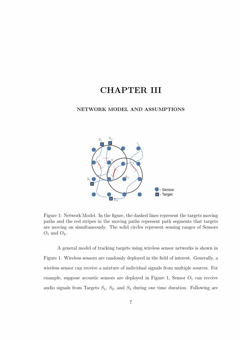
1 Network Model. In the figure, the dashed lines represent the targets

moving paths and the red stripes in the moving paths represent path

segments that targets are moving on simultaneously. The solid circles

represent sensing ranges of Sensors O1 and O2. . . . . . . . . . . . . . 7

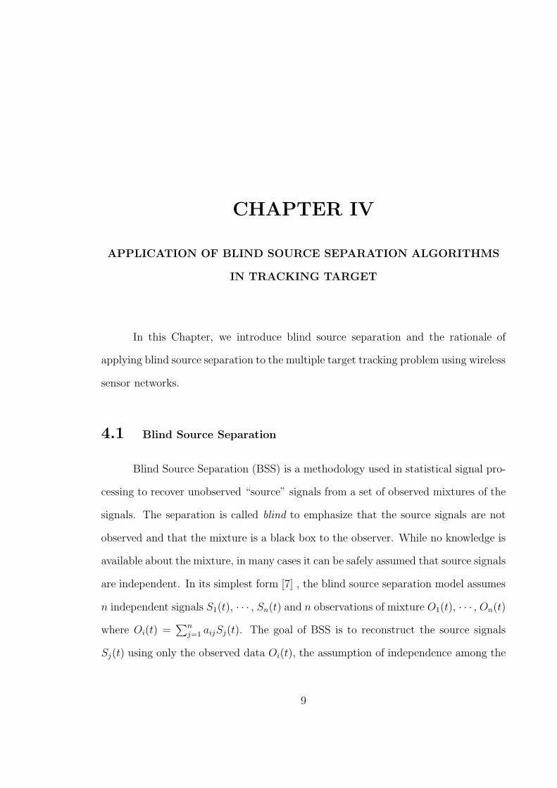
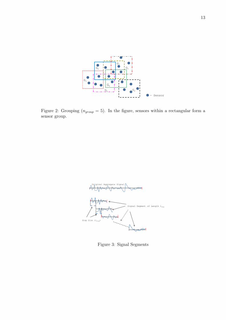
2 Grouping (ngroup = 5). In the figure, sensors within a rectangular form

a sensor group. . . . . . . . . . . . . . . . . . . . . . . . . . . . . . . 13

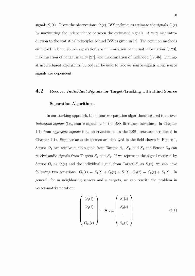
3 Signal Segments . . . . . . . . . . . . . . . . . . . . . . . . . . . . . . 13

4 Rationale Behind The Center Selection Step . . . . . . . . . . . . . . 17

5 Clustering . . . . . . . . . . . . . . . . . . . . . . . . . . . . . . . . . 19

6 Setup for Experiments on Signal Attenuation. In the figure, the solid

line and the dashed lines represent the moving paths taken by the

target of interest and other targets respectively. . . . . . . . . . . . . 27

7 Effect of Attenuation . . . . . . . . . . . . . . . . . . . . . . . . . . . 28

8 Error Distance. The area within the dashed line is the estimated area

and the error distance between a dot within estimated area and the

actual target path is shown in the figure. . . . . . . . . . . . . . . . . 29

9 Empirical Evaluation . . . . . . . . . . . . . . . . . . . . . . . . . . . 34

10 An Example . . . . . . . . . . . . . . . . . . . . . . . . . . . . . . . . 37

11 Effect of BSS Algorithm . . . . . . . . . . . . . . . . . . . . . . . . . 38

x

12 Tracking Performance for Different Sensor Density: with 95 Percent

Confidence Interval . . . . . . . . . . . . . . . . . . . . . . . . . . . . 39

13 Comparison between Experimental Results and Theoretical Results . 40

14 Tracking Performance for Different Number of Targets: with 95 Percent


15 Scatter Plot of Tracking Performance vs. Moving Speed . . . . . . . . 41

16 Effect of Signal Segment Length (lseg) on Tracking Performance: with

95 Percent Confidence Interval . . . . . . . . . . . . . . . . . . . . . . 42

17 Effect of Step Size (lstep) on Tracking Performance: with 95 Percent


18 Effect of Parameter nslot on Tracking Performance: with 95 Percent


19 Effect of Number of Sensors in Sensor Groups: with 95 Percent Confi-

dence Interval . . . . . . . . . . . . . . . . . . . . . . . . . . . . . . . 45

20 Path with High Frequency Variation: with 95 Percent Confidence Interval 45

21 Example of Zigzag Path . . . . . . . . . . . . . . . . . . . . . . . . . 46

22 Effect of Topology on Separation . . . . . . . . . . . . . . . . . . . . 53

23 Example of Cluster Topology . . . . . . . . . . . . . . . . . . . . . . 54

24 Effect of Number of Sensors per Cluster (nclust) with 95 Percent Con-

fidence Interval (When nclust = 1, Cluster Topology essentially degen-

erates into Grid Topology.) . . . . . . . . . . . . . . . . . . . . . . . . 59

25 Effect of In-Cluster Arrangement on Tracking Performance . . . . . . 60

26 Effect of Intra Cluster Distance (dintra) on Tracking Performance with

95 Percent Confidence Interval . . . . . . . . . . . . . . . . . . . . . . 62

27 Finest Tracking Resolution . . . . . . . . . . . . . . . . . . . . . . . . 74

xi

28 Average Tracking Resolution . . . . . . . . . . . . . . . . . . . . . . . 76

xii

List of Algorithms

1 Center Selection Step . . . . . . . . . . . . . . . . . . . . . . . . . . . 20

2 Intersection Step . . . . . . . . . . . . . . . . . . . . . . . . . . . . . . 22

3 Voting Step . . . . . . . . . . . . . . . . . . . . . . . . . . . . . . . . . 24

4 Voting Step (Continued from Algorithm 3) . . . . . . . . . . . . . . . 25

xiii

CHAPTER I

INTRODUCTION

Tracking moving targets with wireless sensors is one of the prominent appli-

cations of wireless sensor networks. Sensors, also called as “smart dust” [47], are

small devices known for their simplicity and low cost. Using a network of sensors

with wireless communication capability enables both cost-effective and performance-

effective approaches to track targets, due to the availability of large amount of data

collected by sensors for tracking targets. Depending on the applications, sensors with

different sensing modalities such as acoustic, seismic, infrared, radio, and magnetic

can be deployed for tracking different type of targets.

In general, data collected by sensors is aggregate data. In the signal processing

language, signals received by sensors are generally mixtures of signals from individual

targets. For example, an acoustic sensor in a field of interest may receive sound

signals from more than one target. Obviously tracking targets based on mixture

signals can result in inaccurate results when interference from targets other than the

one of interest is not negligible. For brevity, we use the term aggregate signal to mean

the signal received by sensor, i.e., data collected by sensors and individual signal to

mean the signal transmitted from or caused by individual targets in the rest of the

1

2

Thesis.

The fact that signals collected by sensor networks are aggregate signals, poses

a big challenge to target-tracking solutions. The problem space of the target-tracking

problem is divided and special cases of the target-tracking problem have been well

studied:

∙ Single-target case: In this case, it is assumed that only one target exists in a

field of interest. So signals received by sensors are essentially individual signals.

∙ Negligible interference case: Some researches assume that interference from

targets other than the one of interest is negligible. The assumption is legitimate

only for applications in which signal from a target attenuates dramatically when

distance between the target and sensor increases.

∙ Distinguishable target case: Sensors can distinguish targets by tags embedded

in signals or by having different targets to send signals using different channels

such as using different frequency bands.

All these special cases assume that tracking algorithms can have access to individual

signals. Singh et al. [52] proposed a general approach to track multiple targets indis-

tinguishable by sensors. The approach is based on binary proximity sensors that can

only report whether or not there are targets in sensing areas. The approach is simple

and robust to interference from other targets with the cost of the limitation that it

is only applicable to track targets in smooth paths [52].

We propose an approach based on Blind Source Separation, a methodology

from statistical signal processing to recover unobserved “source” signals from a set

of observed mixtures of the signals. Blind source separation models were originally

defined to solve the cocktail party problem: The blind source separation algorithms

can extract one person’s voice signal from given mixtures of voices in a cocktail party.

3

Blind source separation algorithms solve the problem based on the independence be-

tween voices from different persons. Similarly, in the target-tracking problem, it is

generally safe to assume individual signals from different targets are independent.

So, we can use blind source separation algorithms to recover individual signals from

aggregate signals collected by sensors. For the cases in which individual signals are

dependent, blind source separation algorithms based on timing structure [56] of indi-

vidual signals can be used.

The proposed algorithm utilizes both temporal information and spatial infor-

mation available to track targets. Applying blind source separation algorithms on

aggregate signals collected by sensors can recover individual signals. But the output

of blind source separation algorithms includes not only recovered individual signals,

but also noise signals, aggregate signals and partial signals, which contain part of

individual signals in different time durations. Clustering is used in our algorithm

to pick out the individual signals from signal output by the blind source separation

algorithms. A voting step based on spatial information is used to further improve the

performance of the algorithm.

The contributions of this Thesis can be summarized as follows:

∙ We proposed a general approach to track multiple targets in a field. The ap-

proach can be applied in real-world applications where targets are indistin-

guishable and interference from targets other than the one of interest is not

negligible.

∙ We evaluate our approach with both empirical experiments and simulations.

We also analyze the effect of parameters used in the proposed approach exper-

imentally and theoretically.

∙ We propose metrics to evaluate performance of target-tracking algorithms. The

metrics originate from the general metrics used to evaluate performance of an

4

estimator in statistics since, essentially, target tracking algorithms estimate the

paths based on data collected from sensor networks.

∙ According to our knowledge, we are the first to apply blind source separation to

process data collected from wireless sensor networks. Blind source separation

algorithms are useful tools for processing data collected from wireless sensor

networks since, essentially, data collected from sensors are all aggregate data.

In this Thesis we focus on applying blind source separation in the target-tracking

problem. The blind source separation algorithms can also be used to process

data in other applications of wireless sensor networks such as location detection

and factor analysis. For most applications of wireless sensor networks, analysis

based on individual signals can yield more accurate results.

1.1 Organization of the Thesis

The rest of the thesis is organized as follows: In Chapter 2, we review related

work. Chapter 3 outlines our network model and assumptions. The main idea of

applying blind source separation algorithms in tracking targets is described in Chapter

4. In Chapter 5, we describe our approach in details. We theoretically analyzed the

performance of our approach and effect of parameters used in our approaches in

Chapter6. The evaluation of our approach by empirical experiments and simulations

is presented in Chapter 7 and Chapter 8 respectively. In Chapter 9 we discuss on

topologies of sensor network to improve tracking performance and formally defines the

problem in randomly placed low-density networks. We describe proposed topologies

in Chapter 10. We evaluate proposed topologies under various settings in Chapter

11. We discuss possible extension to our approach and outline our future work in

Chapter 12. The thesis concludes in Chapter 13.

CHAPTER II

RELATED WORK

Multiple-target tracking originates from military applications such as tracking

missiles and airplanes with radars and tracking vessels with sonars [53]. In these

applications, sensors such as radars and sonars are able to scan a field of interest

with beams operating in selected resolution modes and in selected beam directions.

The tracking systems track targets based on deflection from targets. Algorithms

based on particle filtering and kalman filtering were proposed for these applications

[18, 31, 40, 57, 58]. In this Thesis, we assume simple wireless sensors, which can only

report signal strength and has no capability to determine signal directions, are used

for target tracking.

Wireless sensors, known for their simplicity and low cost, have been proposed

or deployed to track targets in various applications. The examples are tracking robots

with infrared signals [9], tracking vehicles with infrared signals [20], tracking ground

moving targets with seismic signals [43], tracking moving vehicles with acoustic sen-

sors [26], and tracking people with RF signals [45]. Location detection, equivalent to

tracking static targets, has also been studied extensively. This topic has been investi-

gated in different wireless networks such as wireless sensor networks [49,50], wireless

5

6

LANs [2], and wireless ad-hoc networks [12, 61].

Most approaches proposed to track targets or detect location are based on

characteristics of physical signals such as angle of arrival (AOA) [14, 36, 39], Time of

Arrival (TOA) [37,41], Time Difference of Arrival (TDOA) [11,48] and Received Signal

Strength (RSS) [25, 62]. Receiver signal strength is widely used in tracking targets

with wireless sensor networks [2,34]. Most of the previous researches focus on tracking

a single target [1, 16, 29, 42, 51] or assume targets are distinguishable [20, 35, 38, 60].

A string of researches on tracking targets with wireless sensor networks are

based on binary proximity sensors which can only report whether there are targets

within sensing areas. The initial work [1, 29, 51] on binary proximity sensors focuses

on tracking single target. Singh et al. [52] extended the approach to track multiple

indistinguishable targets by applying particle filtering algorithms. Approaches based

on binary proximity sensors have two obvious advantages: (a) The sensors are very

simple since they only report binary information. (b) The approaches are robust since

interference from other targets are essentially filtered out by an equivalent low-pass

filter [51]. The cost of using these simple devices is loss of information that is helpful

to accurately track targets due to the filtering effect. So, approaches based on binary

proximity sensors can not track target in a path with high-frequency variations [51].

We propose a general approach to track multiple indistinguishable targets. The ap-

proach is based on blind source separation algorithms, which can recover individual

signals from aggregate signals. So, the challenging problem of tracking multiple tar-

gets becomes a much easier problem, equivalent to tracking single targets. Since

individual signals can be fully recovered, our approach can track targets following

paths with high-frequency variations.

CHAPTER III

NETWORK MODEL AND ASSUMPTIONS

S2

S3

O1

S4

S1

o2

- Sensor- Target

Figure 1: Network Model. In the figure, the dashed lines represent the targets movingpaths and the red stripes in the moving paths represent path segments that targetsare moving on simultaneously. The solid circles represent sensing ranges of SensorsO1 and O2.

A general model of tracking targets using wireless sensor networks is shown in

Figure 1. Wireless sensors are randomly deployed in the field of interest. Generally, a

wireless sensor can receive a mixture of individual signals from multiple sources. For

example, suppose acoustic sensors are deployed in Figure 1, Sensor O1 can receive

audio signals from Targets S1, S2, and S3 during one time duration. Following are

7

8

the assumptions made in this general model:

∙ Sensors have no capability to distinguish targets. This assumption is important

for deploying sensors in uncooperative or hostile environments such as tracking

enemy soldiers with wireless sensor networks.

∙ The location of each sensor in the sensor network is known. Location informa-

tion can be gathered in a variety of ways. For example, the sensors may be

planted, and their location is marked. Alternatively, sensors may have GPS ca-

pabilities. Finally, sensors may locate themselves through one of several schemes

that rely on sparsely located anchor sensor nodes [6].

∙ Aggregate signals collected by wireless sensors can be gathered for processing

by a sink or gateway. Data compression or coding schemes designed for sensor

networks such as ESPIHT [54,59] can be used to reduce the data volume that is

caused by remaining spatial redundancy across neighboring nodes or temporal

redundancy at individual nodes.

∙ Targets are moving under a speed limit. Obviously it is impossible to track a

high-speed target that only generates a small amount of data when passing the

field of interest. We analyze the effect of the speed limit in Chapter 6.

CHAPTER IV

APPLICATION OF BLIND SOURCE SEPARATION ALGORITHMS

IN TRACKING TARGET

In this Chapter, we introduce blind source separation and the rationale of

applying blind source separation to the multiple target tracking problem using wireless

sensor networks.

4.1 Blind Source Separation

Blind Source Separation (BSS) is a methodology used in statistical signal pro-

cessing to recover unobserved “source” signals from a set of observed mixtures of the

signals. The separation is called blind to emphasize that the source signals are not

observed and that the mixture is a black box to the observer. While no knowledge is

available about the mixture, in many cases it can be safely assumed that source signals

are independent. In its simplest form [7] , the blind source separation model assumes

n independent signals S1(t), ⋅ ⋅ ⋅ , Sn(t) and n observations of mixture O1(t), ⋅ ⋅ ⋅ , On(t)

where Oi(t) =∑n

j=1 aijSj(t). The goal of BSS is to reconstruct the source signals

Sj(t) using only the observed data Oi(t), the assumption of independence among the

9

10

signals Sj(t). Given the observations Oi(t), BSS techniques estimate the signals Sj(t)

by maximizing the independence between the estimated signals. A very nice intro-

duction to the statistical principles behind BSS is given in [7]. The common methods

employed in blind source separation are minimization of mutual information [8, 23],

maximization of nongaussianity [27], and maximization of likelihood [17,46]. Timing-

structure based algorithms [55,56] can be used to recover source signals when source

signals are dependent.

4.2 Recover Individual Signals for Target-Tracking with Blind Source

Separation Algorithms

In our tracking approach, blind source separation algorithms are used to recover

individual signals (i.e., source signals as in the BSS literature introduced in Chapter

4.1) from aggregate signals (i.e., observations as in the BSS literature introduced in

Chapter 4.1). Suppose acoustic sensors are deployed in the field shown in Figure 1,

Sensor O1 can receive audio signals from Targets S1, S2, and S3 and Sensor O2 can

receive audio signals from Targets S2 and S4. If we represent the signal received by

Sensor Oi as Oi(t) and the individual signal from Target Si as Si(t), we can have

following two equations: O1(t) = S1(t) + S2(t) + S3(t), O2(t) = S2(t) + S4(t). In

general, for m neighboring sensors and n targets, we can rewrite the problem in

vector-matrix notation,

⎛

⎜

⎜

⎜

⎜

⎜

⎜

⎜

⎝

O1(t)

O2(t)

...

Om(t)

⎞

⎟

⎟

⎟

⎟

⎟

⎟

⎟

⎠

= Am×n

⎛

⎜

⎜

⎜

⎜

⎜

⎜

⎜

⎝

S1(t)

S2(t)

...

Sn(t)

⎞

⎟

⎟

⎟

⎟

⎟

⎟

⎟

⎠

(4.1)

11

where Am×n is called mixing matrix in the BSS literature. Since the individual signals

are independent from each other - they come from different targets - we can use any of

the algorithms mentioned in Chapter 4.1 to recover individual signals S1(t), ⋅ ⋅ ⋅ , Sn(t).

While the goal of BSS in this context is to re-construct the original signals

Si(t), in practice the separated signals are sometimes only loosely related to the

original signals. We categorize these separated signals into four types, as follows: In

the first case, the separated signal is correlated to actual individual signals Si(t). The

separated signal in this case may have a different sign than the original signal. We

call this type of separated signal an individual separated signal. In the second case,

a separated signal may be correlated to an aggregate of signals from several targets.

This happens when signals from more than two targets can be “heard” by all the

sensors. In such a case, the BSS algorithm would not be able to fully separate the

signal mixture into the individual separated signals. Rather, while some individual

signals can be successfully separated, others remain aggregated. In the third case,

separated signals may be correlated to one original signal in the beginning part and

correlated to another original signal in the rest. We call this type of separated signal

a partial separated signal. This happens when a target moves out of one sensing

range and enters into another sensing range. In the fourth case, separated signals

may represent noise signals.

Noise signals are separated out when neighboring sensors receive different in-

dividual signals from the same target. The difference can be caused by signal atten-

uation or environment noise. BSS algorithms separate the difference as noise signals.

The effect of signal attenuation on separation performance is described in Chapter

6.1.

CHAPTER V

TRACKING ALGORITHM

The tracking algorithm consists of six steps: (1) Aggregate signals collected

from sensors are grouped and segmented and these groups of signal segments are fed to

the second step, the blind source separation step. (2) The blind source separation step

outputs separated signals. As described in Chapter 4, these separated signals contain

individual separated signals, aggregate separated signals, noise signals, and partial

separated signals. (3) The clustering step will cluster these separated signals. (4)

The center selection step selects separated signals that are closest to actual individual

signals from clusters formed in the clustering step. (5) The intersection step estimates

segments of paths based on separated signals selected from the previous step. (6) The

voting step outputs estimated paths by voting on path segments generated in the

intersection step. The details of these six steps (preparation, separation, clustering,

center selection, intersection, voting) are described below.

12

13

G3

G1

G2

G4

G5

G6

G7

- Sensor

Figure 2: Grouping (ngroup = 5). In the figure, sensors within a rectangular form asensor group.

Step Size (lstep)

Original Aggregate Signal

Signal Segment of Length lseg

Figure 3: Signal Segments

14

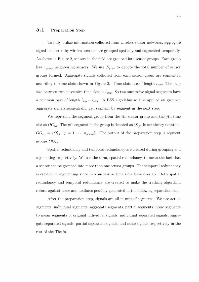
5.1 Preparation Step

To fully utilize information collected from wireless sensor networks, aggregate

signals collected by wireless sensors are grouped spatially and segmented temporally.

As shown in Figure 2, sensors in the field are grouped into sensor groups. Each group

has ngroup neighboring sensors. We use Ngrps to denote the total number of sensor

groups formed. Aggregate signals collected from each sensor group are segmented

according to time slots shown in Figure 3. Time slots are of length lseg. The step

size between two successive time slots is lstep. So two successive signal segments have

a common part of length lseg − lstep. A BSS algorithm will be applied on grouped

aggregate signals sequentially, i.e., segment by segment in the next step.

We represent the segment group from the ith sensor group and the jth time

slot as OGi,j. The pth segment in the group is denoted as Opi,j. In set theory notation,

OGi,j = {Opi,j : p = 1, ⋅ ⋅ ⋅ , ngroup}. The output of the preparation step is segment

groups OGi,j.

Spatial redundancy and temporal redundancy are created during grouping and

segmenting respectively. We use the term, spatial redundancy, to mean the fact that

a sensor can be grouped into more than one sensor groups. The temporal redundancy

is created in segmenting since two successive time slots have overlap. Both spatial

redundancy and temporal redundancy are created to make the tracking algorithm

robust against noise and artifacts possibly generated in the following separation step.

After the preparation step, signals are all in unit of segments. We use actual

segments, individual segments, aggregate segments, partial segments, noise segments

to mean segments of original individual signals, individual separated signals, aggre-

gate separated signals, partial separated signals, and noise signals respectively in the

rest of the Thesis.

15

5.2 Separation Step

In the separation step, a BSS algorithm is applied on segments contained in

OGi,j for all i and j. The outputs of the separation step are groups of separated

segments denoted by SGi,j, i.e., the group of segments separated from OGi,j.

5.3 Clustering Step

The clustering step is designed to eliminate noise segments, aggregate seg-

ments, and partial segments by taking advantage of spatial redundancy created in

the preparation step. The heuristic behind this step is as follows: if a separated

signal represents an individual signal, similar signals will be separated in at least

similar forms by more than one neighboring sensor groups. In contrast, a separated

signal that was generated because of attenuation or interference is unlikely to be

generated by more than one group1. In our experiments, agglomerative hierarchical

clustering [13] is used.

Based on the heuristic, we use correlation as the measure of similarity, and

define the distance between two separated segments as follows:

D(S′pi,j, S

′qk,j) = 1− ∣corr(S ′p

i,j, S′qk,j)∣ , (5.1)

where S′pi,j denotes the pth segment in separated segment group SGi,j, and corr(x, y)

denotes the correlation coefficient of segments x and y. We use the absolute value

of the correlation coefficient because the separated segments may be of different sign

than the actual segment. Clustering will only cluster segments of the same time slots

as indicated in the distance measure defined in Equation 5.1. The number of clusters

formed in this step is heuristically set to two times the number2 of targets in the field

1More analysis of attenuation and interference can be found in Chapter 62The number of targets can be either known a priori or can be estimated using existing algorithms

16

because some clusters may contain only partial segments and noise segments. These

clusters of partial segments and noise segments are removed in the following center

selection step.

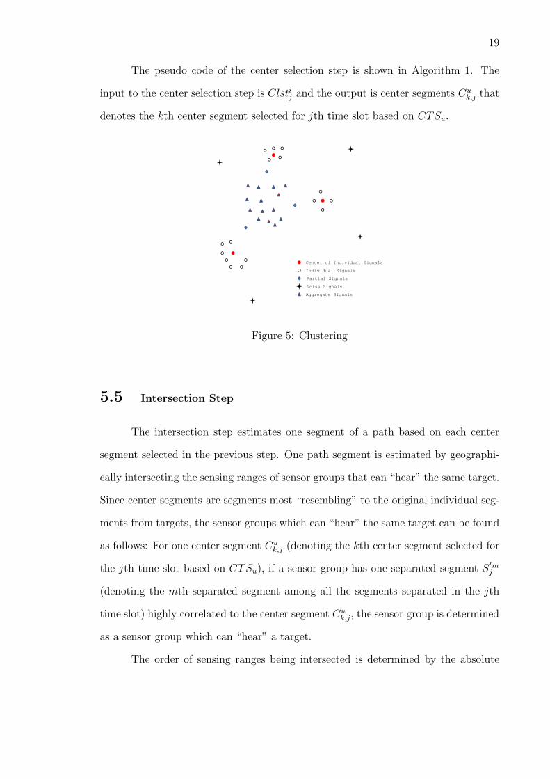
The highly-correlated (similar) segments will cluster together. Figure 5 uses

a two-dimensional representation to further illustrate the rationale for the clustering

approach in this step. In Figure 5, the two-dimensional representation is only for

visualization: Each dot in the figure represents a separated segment of length lseg.

For better visualization, we simplify the visualization to be two-dimension. Since it

is impossible to draw in a space with more than three dimensions. As shown in this

Figure 5, the individual segments form clusters. The aggregate segments and partial

segments, on the other hand, scatter in-between these clusters. The noise segments

are distant both from each other and from the other segments.

In summary, the input of the clustering step is SGi,j and the clustering step

outputs clusters formed in each time slots. We use Clstij to denote the ith cluster

formed in the jth time slot.

5.4 Center Selection Step

The goal of the center selection step is to select center segments as shown in

Figure 5 from clusters formed in the previous step. Center segments are the segments

in the center of each cluster formed according to the distance measure as defined in

Equation 5.1.

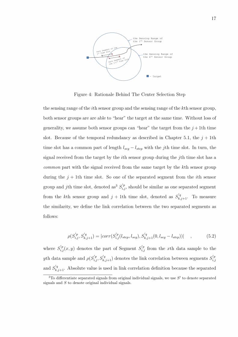
The center selection step is based on the temporal redundancy created in the

preparation step. For ease of understanding, we use the example in Figure 4 to

describe the rationale behind the center selection step. Because of the overlap between

[3, 5, 15]. Similar tracking performance was observed with more clusters mainly because of thefollowing center selection step.

17

the Sensing Range of the ith Sensor Group

the Sensing Range of the kth Sensor Group

- Target

Figure 4: Rationale Behind The Center Selection Step

the sensing range of the ith sensor group and the sensing range of the kth sensor group,

both sensor groups are are able to “hear” the target at the same time. Without loss of

generality, we assume both sensor groups can “hear” the target from the j+1th time

slot. Because of the temporal redundancy as described in Chapter 5.1, the j + 1th

time slot has a common part of length lseg − lstep with the jth time slot. In turn, the

signal received from the target by the ith sensor group during the jth time slot has a

common part with the signal received from the same target by the kth sensor group

during the j + 1th time slot. So one of the separated segment from the ith sensor

group and jth time slot, denoted as3 S′pi,j, should be similar as one separated segment

from the kth sensor group and j + 1th time slot, denoted as S′qk,j+1. To measure

the similarity, we define the link correlation between the two separated segments as

follows:

�(S′pi,j , S

′qk,j+1) = ∣corr(S

′pi,j(lstep, lseg), S

′qk,j+1(0, lseg − lstep))∣ , (5.2)

where S′pi,j(x, y) denotes the part of Segment S

′pi,j from the xth data sample to the

yth data sample and �(S′pi,j, S

′qk,j+1) denotes the link correlation between segments S

′pi,j

and S′qk,j+1. Absolute value is used in link correlation definition because the separated

3To differentiate separated signals from original individual signals, we use S′ to denote separatedsignals and S to denote original individual signals.

18

segments may be of different sign than the actual segments.

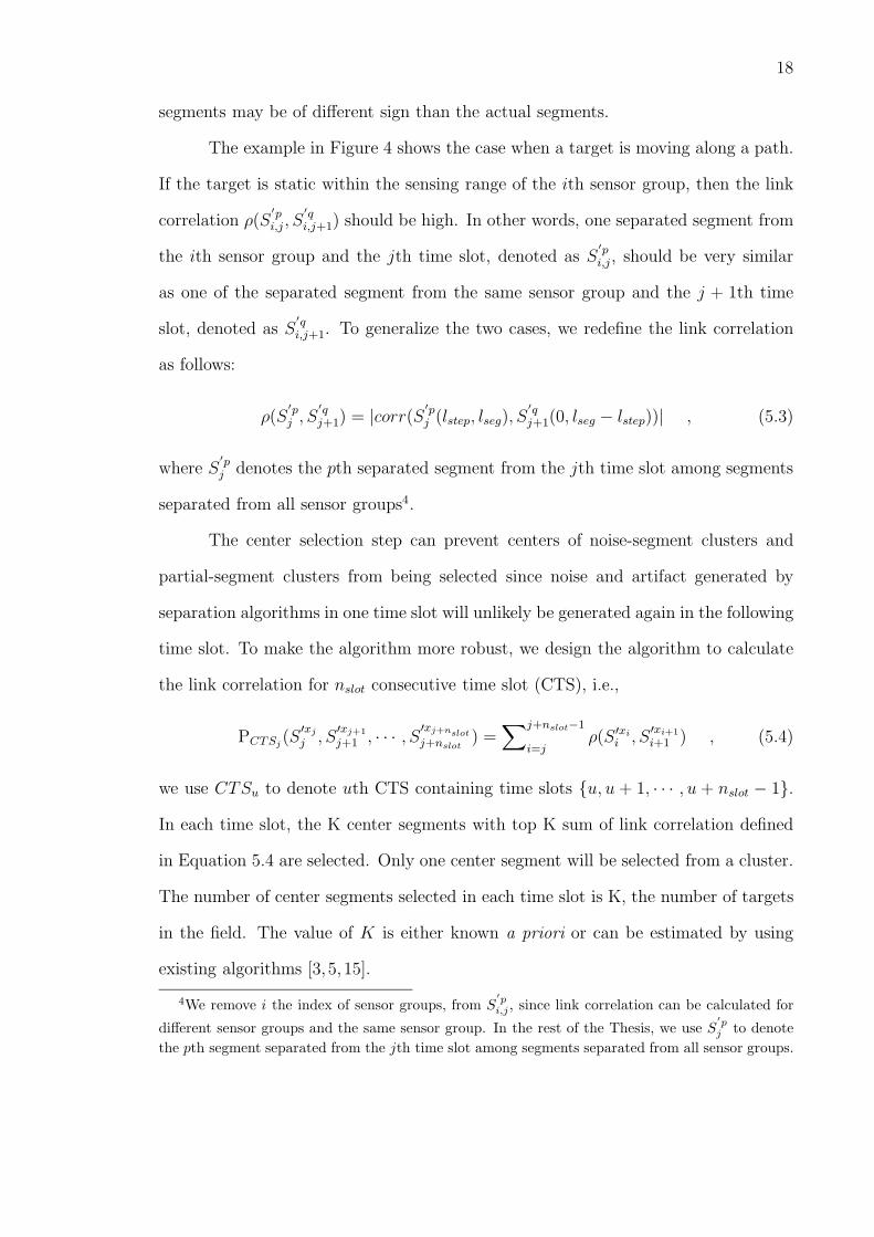
The example in Figure 4 shows the case when a target is moving along a path.

If the target is static within the sensing range of the ith sensor group, then the link

correlation �(S′pi,j , S

′qi,j+1) should be high. In other words, one separated segment from

the ith sensor group and the jth time slot, denoted as S′pi,j, should be very similar

as one of the separated segment from the same sensor group and the j + 1th time

slot, denoted as S′qi,j+1. To generalize the two cases, we redefine the link correlation

as follows:

�(S′pj , S

′qj+1) = ∣corr(S

′pj (lstep, lseg), S

′qj+1(0, lseg − lstep))∣ , (5.3)

where S′pj denotes the pth separated segment from the jth time slot among segments

separated from all sensor groups4.

The center selection step can prevent centers of noise-segment clusters and

partial-segment clusters from being selected since noise and artifact generated by

separation algorithms in one time slot will unlikely be generated again in the following

time slot. To make the algorithm more robust, we design the algorithm to calculate

the link correlation for nslot consecutive time slot (CTS), i.e.,

PCTSj(S

′xj

j , S′xj+1

j+1 , ⋅ ⋅ ⋅ , S ′xj+nslot

j+nslot) =

∑j+nslot−1

i=j�(S ′xi

i , S′xi+1

i+1 ) , (5.4)

we use CTSu to denote uth CTS containing time slots {u, u+ 1, ⋅ ⋅ ⋅ , u+ nslot − 1}.

In each time slot, the K center segments with top K sum of link correlation defined

in Equation 5.4 are selected. Only one center segment will be selected from a cluster.

The number of center segments selected in each time slot is K, the number of targets

in the field. The value of K is either known a priori or can be estimated by using

existing algorithms [3, 5, 15].

4We remove i the index of sensor groups, from S′p

i,j , since link correlation can be calculated for

different sensor groups and the same sensor group. In the rest of the Thesis, we use S′p

j to denote

the pth segment separated from the jth time slot among segments separated from all sensor groups.

19

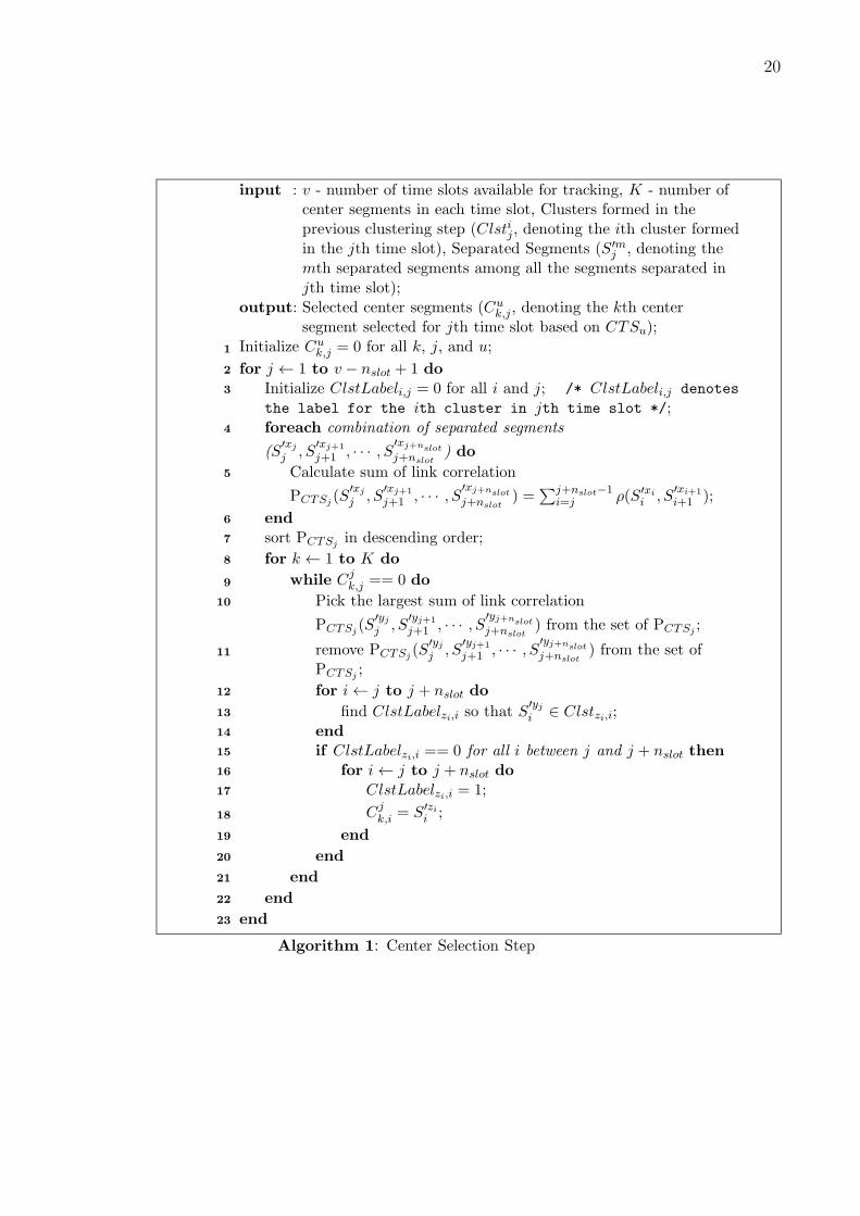
The pseudo code of the center selection step is shown in Algorithm 1. The

input to the center selection step is Clstij and the output is center segments Cuk,j that

denotes the kth center segment selected for jth time slot based on CTSu.vCenter of Individual Signals

Partial Signals

Individual Signals

Partial Signals

Noise Signals

Aggregate Signals

Figure 5: Clustering

5.5 Intersection Step

The intersection step estimates one segment of a path based on each center

segment selected in the previous step. One path segment is estimated by geographi-

cally intersecting the sensing ranges of sensor groups that can “hear” the same target.

Since center segments are segments most “resembling” to the original individual seg-

ments from targets, the sensor groups which can “hear” the same target can be found

as follows: For one center segment Cuk,j (denoting the kth center segment selected for

the jth time slot based on CTSu), if a sensor group has one separated segment S′mj

(denoting the mth separated segment among all the segments separated in the jth

time slot) highly correlated to the center segment Cuk,j, the sensor group is determined

as a sensor group which can “hear” a target.

The order of sensing ranges being intersected is determined by the absolute

20

input : v - number of time slots available for tracking, K - number ofcenter segments in each time slot, Clusters formed in theprevious clustering step (Clstij, denoting the ith cluster formedin the jth time slot), Separated Segments (S′m

j , denoting themth separated segments among all the segments separated injth time slot);

output: Selected center segments (Cuk,j, denoting the kth center

segment selected for jth time slot based on CTSu);Initialize Cu

k,j = 0 for all k, j, and u;1

for j ← 1 to v − nslot + 1 do2

Initialize ClstLabeli,j = 0 for all i and j; /* ClstLabeli,j denotes3

the label for the ith cluster in jth time slot */;foreach combination of separated segments4

(S′xj

j , S′xj+1

j+1 , ⋅ ⋅ ⋅ , S′xj+nslot

j+nslot) do

Calculate sum of link correlation5

PCTSj(S

′xj

j , S′xj+1

j+1 , ⋅ ⋅ ⋅ , S′xj+nslot

j+nslot) =

∑j+nslot−1i=j �(S′xi

i , S′xi+1

i+1 );

end6

sort PCTSjin descending order;7

for k ← 1 to K do8

while Cjk,j == 0 do9

Pick the largest sum of link correlation10

PCTSj(S

′yjj , S

′yj+1

j+1 , ⋅ ⋅ ⋅ , S′yj+nslot

j+nslot) from the set of PCTSj

;

remove PCTSj(S

′yjj , S

′yj+1

j+1 , ⋅ ⋅ ⋅ , S′yj+nslot

j+nslot) from the set of11

PCTSj;

for i← j to j + nslot do12

find ClstLabelzi,i so that S′yji ∈ Clstzi,i;13

end14

if ClstLabelzi,i == 0 for all i between j and j + nslot then15

for i← j to j + nslot do16

ClstLabelzi,i = 1;17

Cjk,i = S′zi

i ;18

end19

end20

end21

end22

end23

Algorithm 1: Center Selection Step

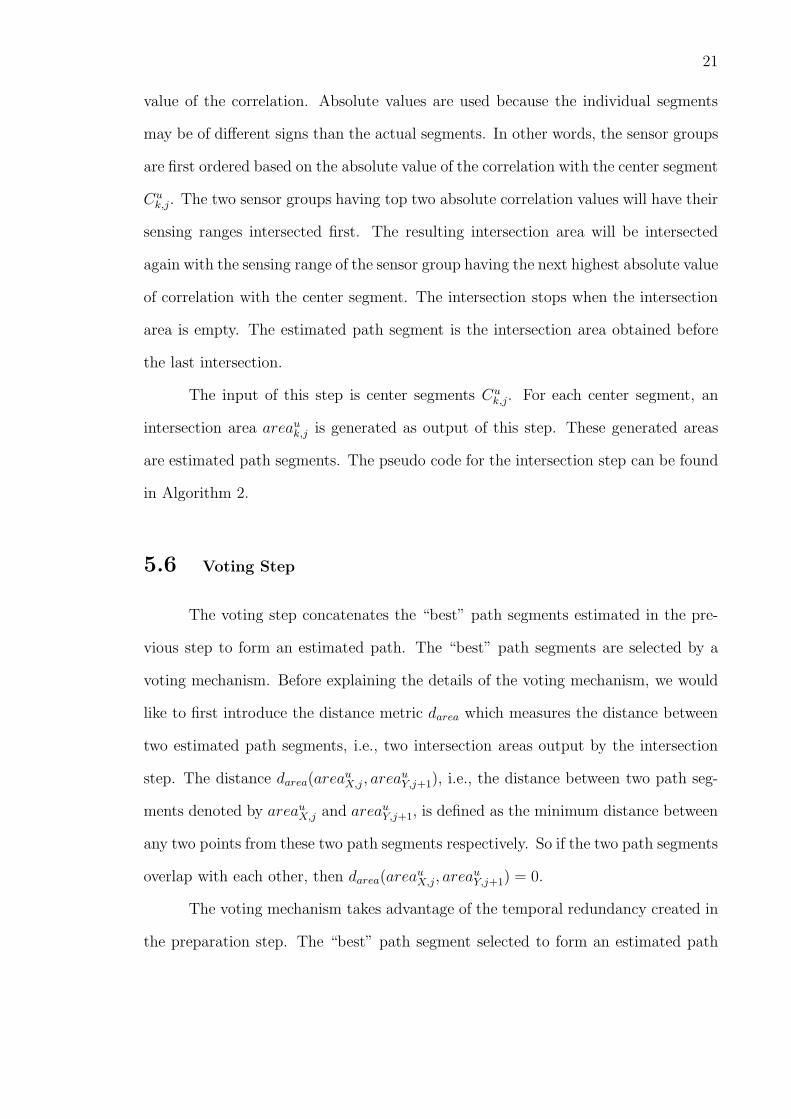
21

value of the correlation. Absolute values are used because the individual segments

may be of different signs than the actual segments. In other words, the sensor groups

are first ordered based on the absolute value of the correlation with the center segment

Cuk,j. The two sensor groups having top two absolute correlation values will have their

sensing ranges intersected first. The resulting intersection area will be intersected

again with the sensing range of the sensor group having the next highest absolute value

of correlation with the center segment. The intersection stops when the intersection

area is empty. The estimated path segment is the intersection area obtained before

the last intersection.

The input of this step is center segments Cuk,j. For each center segment, an

intersection area areauk,j is generated as output of this step. These generated areas

are estimated path segments. The pseudo code for the intersection step can be found

in Algorithm 2.

5.6 Voting Step

The voting step concatenates the “best” path segments estimated in the pre-

vious step to form an estimated path. The “best” path segments are selected by a

voting mechanism. Before explaining the details of the voting mechanism, we would

like to first introduce the distance metric darea which measures the distance between

two estimated path segments, i.e., two intersection areas output by the intersection

step. The distance darea(areauX,j , area

uY,j+1), i.e., the distance between two path seg-

ments denoted by areauX,j and areauY,j+1, is defined as the minimum distance between

any two points from these two path segments respectively. So if the two path segments

overlap with each other, then darea(areauX,j, area

uY,j+1) = 0.

The voting mechanism takes advantage of the temporal redundancy created in

the preparation step. The “best” path segment selected to form an estimated path

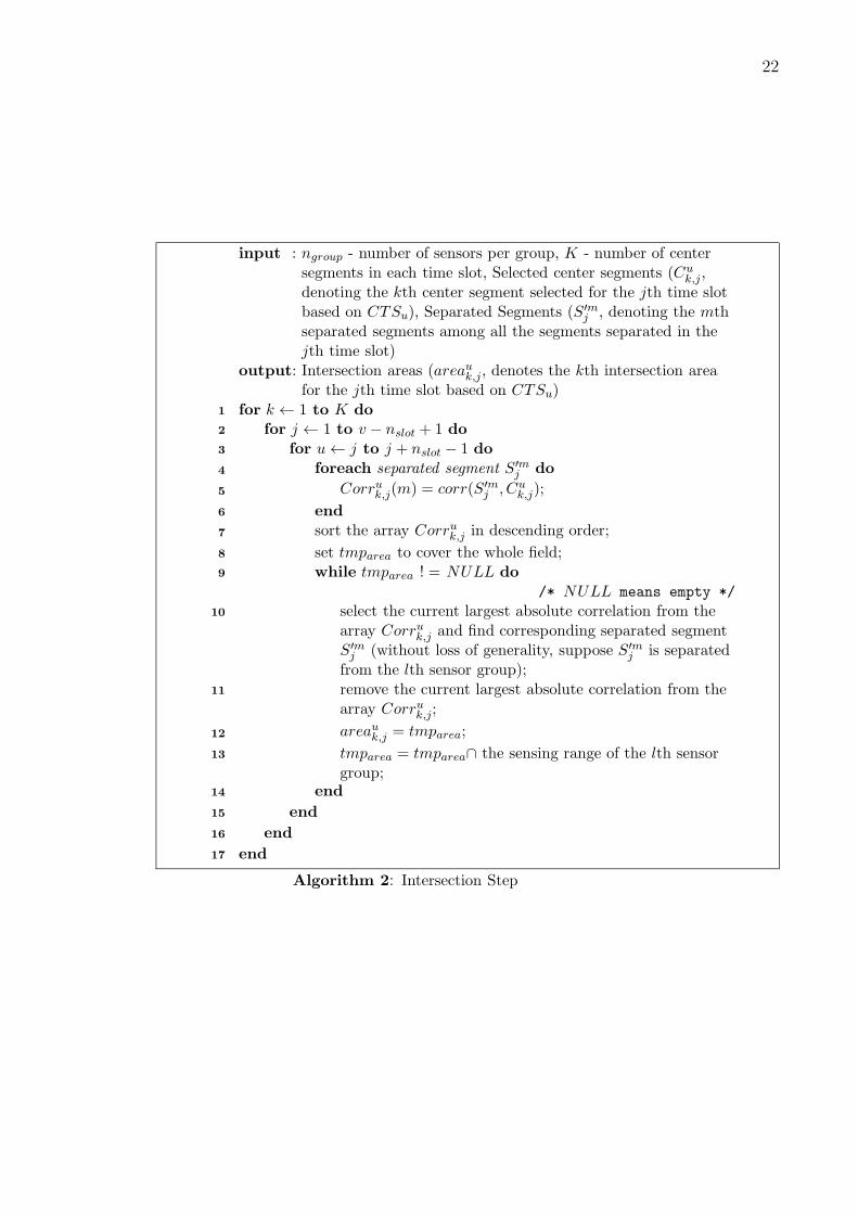
22

input : ngroup - number of sensors per group, K - number of centersegments in each time slot, Selected center segments (Cu

k,j,denoting the kth center segment selected for the jth time slotbased on CTSu), Separated Segments (S′m

j , denoting the mthseparated segments among all the segments separated in thejth time slot)

output: Intersection areas (areauk,j, denotes the kth intersection areafor the jth time slot based on CTSu)


for j ← 1 to v − nslot + 1 do2

for u← j to j + nslot − 1 do3

foreach separated segment S′mj do4

Corruk,j(m) = corr(S′mj , Cu

k,j);5

end6

sort the array Corruk,j in descending order;7

set tmparea to cover the whole field;8

while tmparea ! = NULL do9

/* NULL means empty */

select the current largest absolute correlation from the10

array Corruk,j and find corresponding separated segmentS′mj (without loss of generality, suppose S′m

j is separatedfrom the lth sensor group);remove the current largest absolute correlation from the11

array Corruk,j;

areauk,j = tmparea;12

tmparea = tmparea∩ the sensing range of the lth sensor13

group;end14

end15

end16

end17

Algorithm 2: Intersection Step

23

should satisfy the following two requirements: (1) The selected path segment areauk,u

should have zero distance with all path segments estimated based on the same CTSu,

i.e., dcurk,u =∑u+nslot−2

j=u darea(areauk,u, area

uk,j+1) = 0. The selected path segment

should also have zero distance with all the path segments estimated for the same

time slot based on different CTS, i.e.,

dprek,u =∑

min(darea(areauk,u, area

u−m1,u ), ⋅ ⋅ ⋅ , darea(areauk,u, areau−m

K,u )) = 0.

Finally a path is estimated by linking path segments selected from different

time slots. To determine whether a selected “best” path segment, say Psegzj ,j denot-

ing the zjth selected path segment for the jth time slot, belongs to a path, say epatℎl

denoting the lth estimated path, the distance between Psegzj,j and the path segment

of epatℎl determined in the previous time slot, say Psegzj−1,j−1, is calculated. If the

distance is zero, then Psegzj ,j is determined as one path segment of epatℎl. The

pseudo code of the voting step is shown in Algorithm 3 and Algorithm 4.

24

input : K - number of estimated segments in each time slot, v - number oftime slots available, Estimated path segments (areaui,j - the ithestimated segment among all the estimated segments in the jthtime slot based on CTSu;

output: epatℎl - Estimated path of the lth moving target.for u← 1 to v − nslot + 1 do1


dcurk,u =∑u+nslot−2

j=u darea(areauk,u, area

uk,j+1);3

/* dcurk,u is sum of distance between estimated segments

in the uth time slot and other time slots estimated in

the same CTSu. */

if u > 1 && u < nslot then4

/* Boundary Case */

dprek,u =∑u−1

m=1min(darea(areauk,u, area

u−m1,u ),

darea(areauk,u, area

u−m2,u ), ⋅ ⋅ ⋅ ,


u−mK,u ));

/* dprek,u is

5

sum of minimum distance between estimated segments in

the uth time slot in current CTS and the uth time

slot in all previous CTS. */

else6

dprek,u =∑nslot−1

m=1 min(darea(areauk,u, area

u−m1,u ),


u−m2,u ), ⋅ ⋅ ⋅ ,


u−mK,u ));7

end8

if dcurk,u == 0 && dprek,u == 0 then9

Psegk,u = areauk,u; /* Psegk,u, denote the kth estimated10

segment in the uth time slot */

else11

Psegk,u = −1; /* −1, means not selected */;12

end13

if u == v − nslot + 1 then14

for i← u to v − 1 do15

if darea(areauk,u, area

uk,i+1) == 0 then16

Psegk,i+1 = areauk,i+1;17

else18

Psegk,i+1 = −1;19

end20

end21

end22

end23

end24

/* Continuation of Voting Step is shown in Algorithm 4 */

Algorithm 3: Voting Step

25

/* Continuation of Voting Step */

foreach target l← 1 to K do25

for j ← 2 to v do26

if j == 2 then27

ifmin(darea(Psegl,j , Pseg1,j+1), darea(Psegl,j,

Pseg2,j+1), ⋅ ⋅ ⋅ , darea(Psegl,j , PsegK,j+1)) == 028

then

Psegl,j ∈ epatℎl;29

Psegzj+1,j+1 ∈ epatℎl; /* Without loss of generality,30

it is assumed that darea(Psegl,j , Psegzj+1,j+1) = 0. If

more than two segments have zero distance with

Psegl,j, the tiebreaker is the index x in Psegx,j+1.

*/else31

Psegl,j ∈ epatℎl;32

end33

else34

ifmin(darea(Psegzj−1,j−1, Pseg1,j), darea(Psegzj−1,j−1,

Pseg2,j), ⋅ ⋅ ⋅ , darea(Psegzj−1,j−1, PsegK,j)) == 035

then

Psegzj ,j ∈ epatℎl ; /* Without loss of generality, it36

is assumed that darea(Psegzj−1,j−1, Psegzj ,j) = 0 */

end37

end38

if Psegzj ,j ∈ epatℎl then39

continue;40

else41

find the last determined segment in Psegzx,x in epatℎl;42

findmin(darea(Psegzx,x, Pseg1,j), darea(Psegzx,x,

Pseg2,j), ⋅ ⋅ ⋅ , darea(Psegzx,x, PsegK,j));43

Psegzj ,j ∈ epatℎl; /* with out loss of generality, it is

assumed that darea(Psegzx,x, Psegzj ,j) = 0 */

end44

end45

end46

Algorithm 4: Voting Step (Continued from Algorithm 3)

CHAPTER VI

THEORETICAL ANALYSIS

In this Chapter, we analyze the effect of signal attenuation, the tracking reso-

lution, and the effect of moving speed.

6.1 Signal Attenuation

Signal attenuation is a natural consequence of signal transmission over long

distances. It is a function of transmission distance.

When static targets are being tracked, signal attenuation will not affect track-

ing performance. Since targets are static, the distance between targets and sensors

does not change over time. So the attenuation can be modeled as a constant. For

the same individual signal from a target, different sensors will observe different at-

tenuation because of different transmission distance. So individual signals received

by different sensors from the same target are different only by a scaling factor. The

difference because of the scaling factor can be absorbed by the mixing matrix defined

in the BSS model as Equation 4.1. So attenuation does not affect tracking static

targets by our approach.

26

27

d

Center

Path

- Sensor

- Center of a Sensor Group

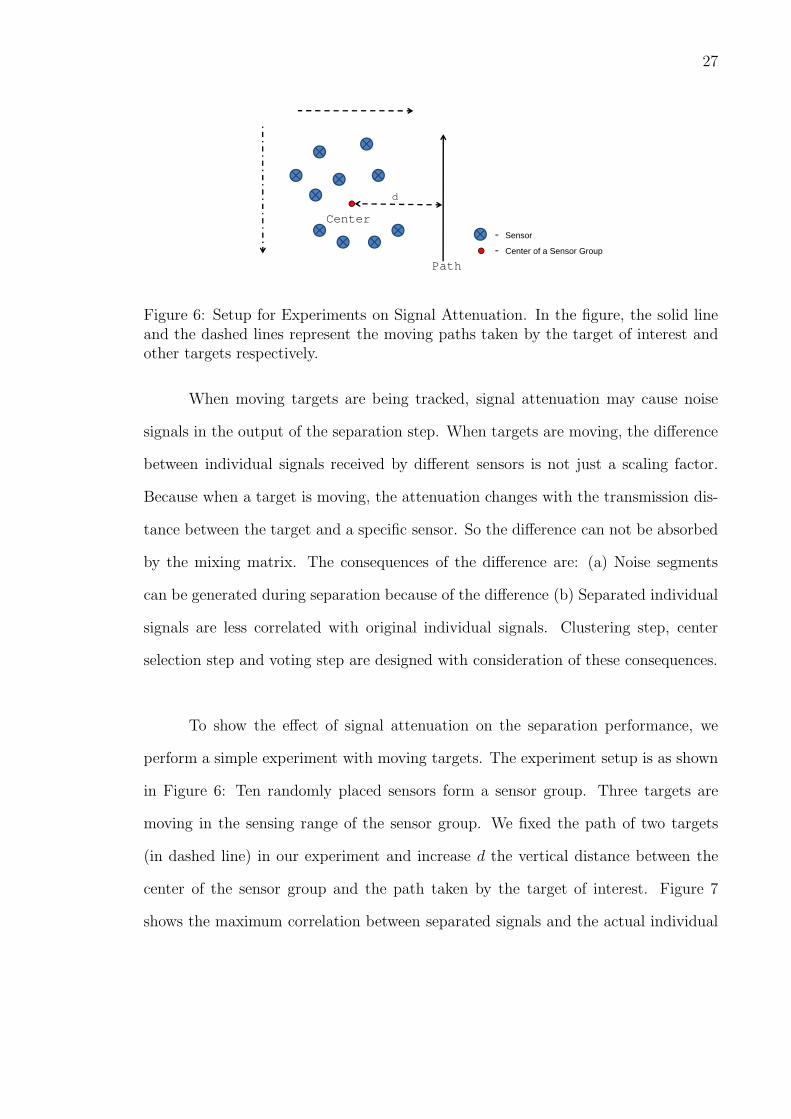
Figure 6: Setup for Experiments on Signal Attenuation. In the figure, the solid lineand the dashed lines represent the moving paths taken by the target of interest andother targets respectively.

When moving targets are being tracked, signal attenuation may cause noise

signals in the output of the separation step. When targets are moving, the difference

between individual signals received by different sensors is not just a scaling factor.

Because when a target is moving, the attenuation changes with the transmission dis-

tance between the target and a specific sensor. So the difference can not be absorbed

by the mixing matrix. The consequences of the difference are: (a) Noise segments

can be generated during separation because of the difference (b) Separated individual

signals are less correlated with original individual signals. Clustering step, center

selection step and voting step are designed with consideration of these consequences.

To show the effect of signal attenuation on the separation performance, we

perform a simple experiment with moving targets. The experiment setup is as shown

in Figure 6: Ten randomly placed sensors form a sensor group. Three targets are

moving in the sensing range of the sensor group. We fixed the path of two targets

(in dashed line) in our experiment and increase d the vertical distance between the

center of the sensor group and the path taken by the target of interest. Figure 7

shows the maximum correlation between separated signals and the actual individual

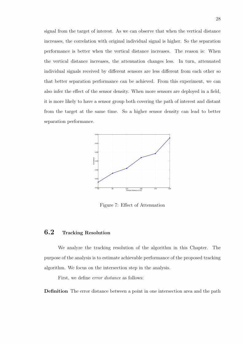
28

signal from the target of interest. As we can observe that when the vertical distance

increases, the correlation with original individual signal is higher. So the separation

performance is better when the vertical distance increases. The reason is: When

the vertical distance increases, the attenuation changes less. In turn, attenuated

individual signals received by different sensors are less different from each other so

that better separation performance can be achieved. From this experiment, we can

also infer the effect of the sensor density. When more sensors are deployed in a field,

it is more likely to have a sensor group both covering the path of interest and distant

from the target at the same time. So a higher sensor density can lead to better

separation performance.

50 80 110 140 170 2000.82

0.84

0.86

0.88

0.90

0.92

0.94

Vertical Distance d (m)

Cor

rela

tion

Figure 7: Effect of Attenuation

6.2 Tracking Resolution

We analyze the tracking resolution of the algorithm in this Chapter. The

purpose of the analysis is to estimate achievable performance of the proposed tracking

algorithm. We focus on the intersection step in the analysis.

First, we define error distance as follows:

Definition The error distance between a point in one intersection area and the path

29

Actual Target Path

Estimated Area

Error Distance

Figure 8: Error Distance. The area within the dashed line is the estimated area andthe error distance between a dot within estimated area and the actual target path isshown in the figure.

of interest is the minimal distance between the point and any point on the path.

Mathematically, the error distance derr between a point (x,y) in an estimated

area A and an actual target path P is defined as follows:

derr(x, y) = min(xp ,yp)∈P ∣(x, y)− (xp, yp)∣2 , (6.1)

where (xp, yp) represent a point on the actual target path P and ∣ ∣2 denotes the

L2-norm.

Tracking resolution is defined based on the error distance definition:

Definition Tracking resolution is defined as the average of error distance between

all the points inside an intersection area and a path segment of interest.

Mathematically, the tracking resolution TR is defined as follows:

TR =

∫

(x,y)∈Aderr(x, y)dxdy

∫

(x,y)∈Adxdy

. (6.2)

As in Figure 8, error distance derr is the minimum distance between the point inside

estimated intersection area (represented with dot) and points on the path segment of

interest. Tracking resolution is the average error distance of all the points inside an

estimated intersection area.

We focus on linear path segments in theoretical analysis for the following rea-

sons: (a) Any path can be formed with linear segments. (b) In practice the size of

30

signal segment used in the proposed algorithm is small so that estimated path seg-

ments are close to linear. To simplify the analysis of the tracking resolution we assume

the path segment of interest fits inside the intersection area and it is perpendicular

to the line joining centers of two sensor groups. We assume the sensors are uniformly

distributed over the field. So sensor groups are also uniformly distributed over the

field.

We assume N sensors are deployed in a field of size a meter by b meter and

the sensing range of each sensor is R. Both the average tracking resolution and the

finest tracking resolution are analyzed below.

6.2.1 Finest Tracking Resolution

The finest tracking resolution is defined as the achievable minimal mean error

distance. We assume sensor groups are located within circles of radius r on average.

So we have

Sensor Density =N

a× b

=ngroup

�r2

where ngroup is the number of sensors in each sensor group. Thus the average radius

r is

r =

√

ngroupab

�N, (6.3)

Theorem 6.2.1 The finest tracking resolution of tracking a linear path segment of

length l is (R+r)2

4lsin−1( l

2(R+r))− 1

8

√

(R + r)2 − ( l2)2.

The proof of Theorem 6.2.1 can be found in Appendix .1.

31

Corollary 6.2.2 When the finest tracking resolution is achieved, the distance between

the two neighboring sensor blocks is 2√

(R + r)2 − ( l2)2

Corollary 6.2.2 can be easily proven by extending Equation 1 in Theorem 6.2.1.

6.2.2 Average Tracking Resolution

The average tracking resolution predicts the average tracking accuracy achiev-

able by the proposed tracking algorithm. It is the mean error distance averaged over

all the possible cases.

Theorem 6.2.3 The average tracking resolution of tracking a linear path segment of

length l is (R+r)2

4l2sin−1( l

2(R+r))((R + r)− 2

√

(R + r)2 − ( l2)2) + 3(R+r)2

16l− l

16.

The proof of Theorem 6.2.3 can be found in Appendix .2.

6.3 Effect of Moving Speed

In general, targets’ moving speed affects performance of tracking algorithms.

Tracking algorithms track moving targets by observing changes in sensing signals

collected from sensors. If a target moves through a sensor-deployed field with very

high speed, then sensors are not able to observe enough change in sensing signals for

tracking. On the other hand, signals reported by sensors are digitized, i.e., sampled

from original sensing signals. If a sensor can sample sensing signals with a high

sampling rate, the sensing data collected from sensors can possibly capture enough

changes for tracking fast-moving targets. To make moving speed discussed in this

Thesis independent from the sampling rate, we use meter per sample interval as the

unit for speed.

32

Low moving speed leads to better tracking performance. Since when a target

is moving at low speed, more data samples can be collected from sensors. In the sepa-

ration step, the separation performance for longer signal segments is generally better

than the performance for shorter segments. So, in turn, better tracking performance

can be achieved.

CHAPTER VII

EMPIRICAL EVALUATION

We evaluate the proposed tracking algorithm using data [32] collected from

Mica2-compatible XSM motes, programmed using the nesC programming language

and running the TinyOS operating system. The data was collected during simulta-

neous tracking of multiple targets as explained in [33].

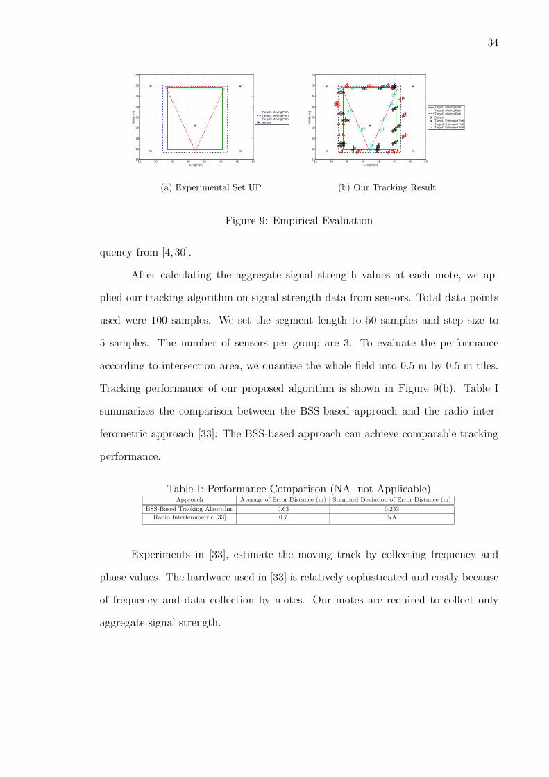
Experimental set up is as shown in Figure 9(a). Five anchor nodes were placed

at known positions, covering an area of approximately 27.4 meter by 27.4 meter. Four

anchor nodes were placed in the corners of the square and the fifth anchor close to

the center. The moving paths of targets are, a person holds two motes in two hands

and walks on the rectangular track and another person holds single mote and walks

on the triangular track. Sensors record the phase and frequency of an interference

signals transmitted over 22 channels.

The signal strength of aggregate signals received by sensors can be calculated

as follows:

signal strength =

22∑

i=1

distance

att× alpℎa, (7.1)

where att is attenuation and alpℎa is attenuation coefficient calculated using fre-

33

34

15 20 25 30 35 40 45 5015

20

25

30

35

40

45

50

55

Length (m)

Wid

th (

m)

Target1 Moving PathTarget2 Moving PathTarget3 Moving PathSensor

15 20 25 30 35 40 45 5015

20

25

30

35

40

45

50

55

Length (m)

Wid

th (

m)

Target1 Moving PathTarget2 Moving PathTarget3 Moving PathSensorTarget1 Estimated PathTarget2 Estimated PathTarget3 Estimated Path

(a) Experimental Set UP (b) Our Tracking Result

Figure 9: Empirical Evaluation

quency from [4, 30].

After calculating the aggregate signal strength values at each mote, we ap-

plied our tracking algorithm on signal strength data from sensors. Total data points

used were 100 samples. We set the segment length to 50 samples and step size to

5 samples. The number of sensors per group are 3. To evaluate the performance

according to intersection area, we quantize the whole field into 0.5 m by 0.5 m tiles.

Tracking performance of our proposed algorithm is shown in Figure 9(b). Table I

summarizes the comparison between the BSS-based approach and the radio inter-

ferometric approach [33]: The BSS-based approach can achieve comparable tracking

performance.

Table I: Performance Comparison (NA- not Applicable)Approach Average of Error Distance (m) Standard Deviation of Error Distance (m)

BSS-Based Tracking Algorithm 0.63 0.253Radio Interferometric [33] 0.7 NA

Experiments in [33], estimate the moving track by collecting frequency and

phase values. The hardware used in [33] is relatively sophisticated and costly because

of frequency and data collection by motes. Our motes are required to collect only

aggregate signal strength.

CHAPTER VIII

PERFORMANCE EVALUATION

We evaluate the performance of the proposed tracking algorithm with extensive

simulations. We assume acoustic sensors are deployed in the field of interest for

tracking purpose.

8.1 Experiment Setup

In the following experiments, the simulated field is a 1600m × 1600m square

area. Sensors are randomly deployed in the field. The movement of targets is re-

stricted to a 1000m × 1000m center area to eliminate boundary effects. The signals

used for tracking are real bird signals downloaded from the website of Florida Museum

of Natural History [21]. In our simulation experiments, we use FastICA [24] algorithm

for signal separation. FastICA is an efficient and popular algorithm for independent

component analysis in terms of accuracy and low computational complexity. The at-

tenuation of sound signals is according to atmospheric sound absorption model [4,30].

The simulations are performed in Matlab. Following parameters are used in our ex-

periments if not specified: (1) The sensing range of sensors is 250m. (2) Paths followed

35

36

by targets are generated randomly. (3) The number of sensors in each sensor group

ngroup is 10. (4) The number of moving targets in the field is 10. (5) Sensor density

is sensors in the field. (6) The segment length is 100 samples and the step size is 10

samples. (7) Targets are moving at a speed below 0.15 meter per sample interval.

8.2 Performance Metrics

As described in Chapter 5.5 and 5.6, the estimated paths output by the target-

tracking algorithm is essentially concatenated intersection areas. To evaluate the

performance according to the concatenated intersection areas, we quantize the whole

area using 5m × 5m tiles. One intersection area is represented by a set of points

inside the area, each point representing the corner of the corresponding tile. Two

metrics are used to evaluate the area: One is the mean error distance. It is based

on the error distance defined in Chapter 6.2. The mean error distance is the mean

of the error distance between all points inside concatenated intersection areas and

the actual path taken by a target. The other is the standard deviation of the error

distance between the points inside the concatenated intersection areas and the actual

path taken by a target. The first one measures accuracy of the tracking algorithm and

the second measures precision of the tracking algorithm. If we cast the evaluation of

the estimation algorithm in terms of evaluating a statistical estimator, the accuracy

corresponds to the bias of the estimator and the precision corresponds to the variance

of the estimator.

The step size can affect both tracking performance and computational com-

plexity. A big step size can reduce computation time with the cost of having gaps

between concatenated intersection areas. We use percentage of coverage to measure

the continuity in estimated paths. It is equal to one minus the ratio between the

sum of distance between neighboring intersection areas and the length of the actual

37

0 200 400 600 800 1000 1200 1400 16000

200

400

600

800

1000

1200

1400

1600

sensortaget1target2target3target4target5target6target7target8target9

0 200 400 600 800 1000 1200 1400 16000

200

400

600

800

1000

1200

1400

1600

(a) Experiment Setup (b) Tracking Result

Figure 10: An Example

path. The distance between two intersection areas is defined as in Chapter 5.6: It is

the distance between two closest points in each intersection area. If two intersection

areas have overlap, the distance is zero.

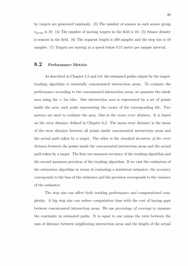
8.3 A Typical Example

An example of typical results of the proposed tracking algorithm is shown in

Figure 10. The paths taken by these targets are shown in Figure 10(a). The sensor

density is 1000 sensors in the field. We include a zigzag1 path in this example since

the zigzag path is one kind of path with high frequency variation. Figure 10(b)

shows paths estimated by our algorithm. The estimated paths are drawn in red dots.

We can observe from the Figure 10 that the proposed tracking algorithm can track

targets including targets following paths with high frequency variations, accurately

and precisely.

1A formal definition of zigzag path is given in the Chapter 8.12 on experiments of paths withhigh frequency variation.

38

8.4 Effectiveness of BSS Algorithm

In this Chapter we investigate the relationship between the effectiveness of the

BSS algorithms and tracking performance. In this set of experiments the number of

moving targets is 10 and the sensor density is 1000 sensors in the field. Figure 11 show

the relationship between separation performance and tracking performance. The X-

axis is absolute value of correlation between center components selected in center

selection step and original signals. A large value in X-axis indicates better separa-

tion performance. Y-axis is mean of error distance, measuring tracking performance.

Figure 11 shows tracking performance increases with separation performance.

0.3 0.4 0.5 0.6 0.7 0.8 0.9 10

5

10

15

20

25

30

Correlation

Mea

n of

Err

or D

ista

nce

(m)

Figure 11: Effect of BSS Algorithm

8.5 Sensor Density vs Performance

As analyzed in Chapter 6, sensor density can greatly affect tracking perfor-

mance. In this series of experiments, we increase the number of sensors in the field

from 100 to 1000.

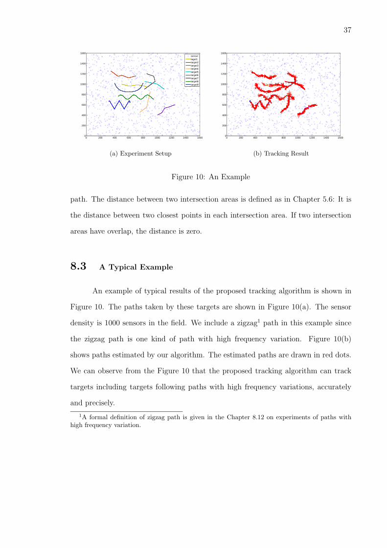
Figure 12(a) and 12(b) shows the tracking performance under different sensor

densities. From Figure 12(a), we can observe: (a) The tracking algorithm can both

39

100 200 300 400 500 600 700 800 900 10000

5

10

15

20

25

30

35

Sensor Density

Err

or D

ista

nce

(m)

Mean of Error DistanceStandard Deviation of Error Distance

100 200 300 400 500 600 700 800 900 100082

84

86

88

90

92

94

96

98

100

Sensor Density

Per

cent

age

of C

over

age

(a) Error Distance (b) Percentage of Coverage

Figure 12: Tracking Performance for Different Sensor Density: with 95 Percent Con-fidence Interval

accurately and precisely track targets even when the sensor density is not high. (b)

When the sensor density increases, the error distance decreases. This is because of two

reasons: (a) When sensor density increases, more sensor groups can sense the target of

interest. So intersecting sensing areas of more sensor groups can lead to smaller error

distance. (b) When sensor density is high, better separation is possible as analyzed in

Chapter 6.1. Figure 12(b) shows that percentage of coverage decreases when sensor

density increases. In other words, when the sensor density increases, more gaps exist

in the estimated paths. It is because of smaller or more precise intersection areas are

estimated when sensor density increases. So the distance between two neighboring

estimated path segments increases and more gaps are created in this way.

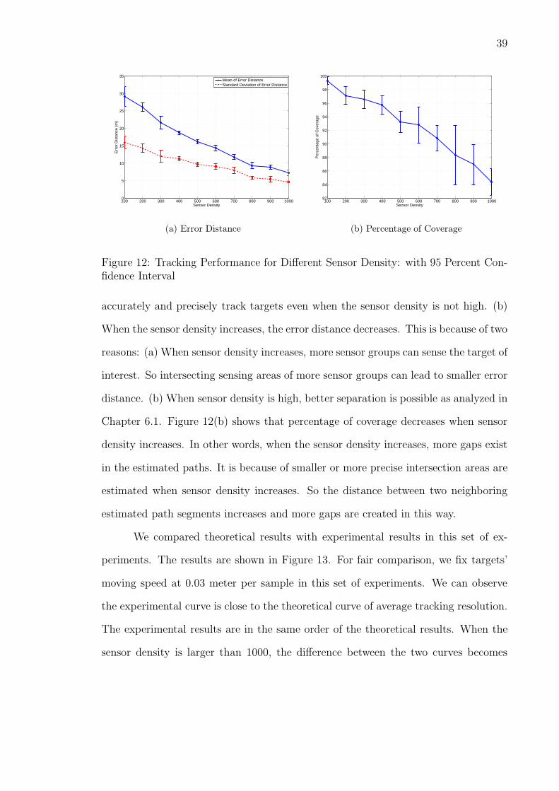
We compared theoretical results with experimental results in this set of ex-

periments. The results are shown in Figure 13. For fair comparison, we fix targets’

moving speed at 0.03 meter per sample in this set of experiments. We can observe

the experimental curve is close to the theoretical curve of average tracking resolution.

The experimental results are in the same order of the theoretical results. When the

sensor density is larger than 1000, the difference between the two curves becomes

40

100 200 300 400 500 600 700 800 900 10004

6

8

10

12

14

16

18

20

22

Sensor Density

Err

or D

ista

nce

(m)

ExperimentalTheoretical

Figure 13: Comparison between Experimental Results and Theoretical Results

5 10 15 20 25 300

5

10

15

20

25

30

35

40

Number of Targets

Err

or D

ista

nce

(m)

Mean of Error Distance−400 sensorsMean of Error Distance−700 sensorsMean of Error Distance−1000 sensorsStandard Deviation of Error Distance−400 sensorsStandard Deviation of Error Distance−700 sensorsStandard Deviation of Error Distance−1000 sensors

5 10 15 20 25 3065

70

75

80

85

90

95

100

Number of Targets

Per

cent

age

of C

over

age

400 sensors700 sensors1000 sensors


Figure 14: Tracking Performance for Different Number of Targets: with 95 PercentConfidence Interval

smaller because (1) Error distance decreases when sensor density increases for both

curves. (2) The difference between these two curves is less than 9 meters when sensor

density is larger than 1000.

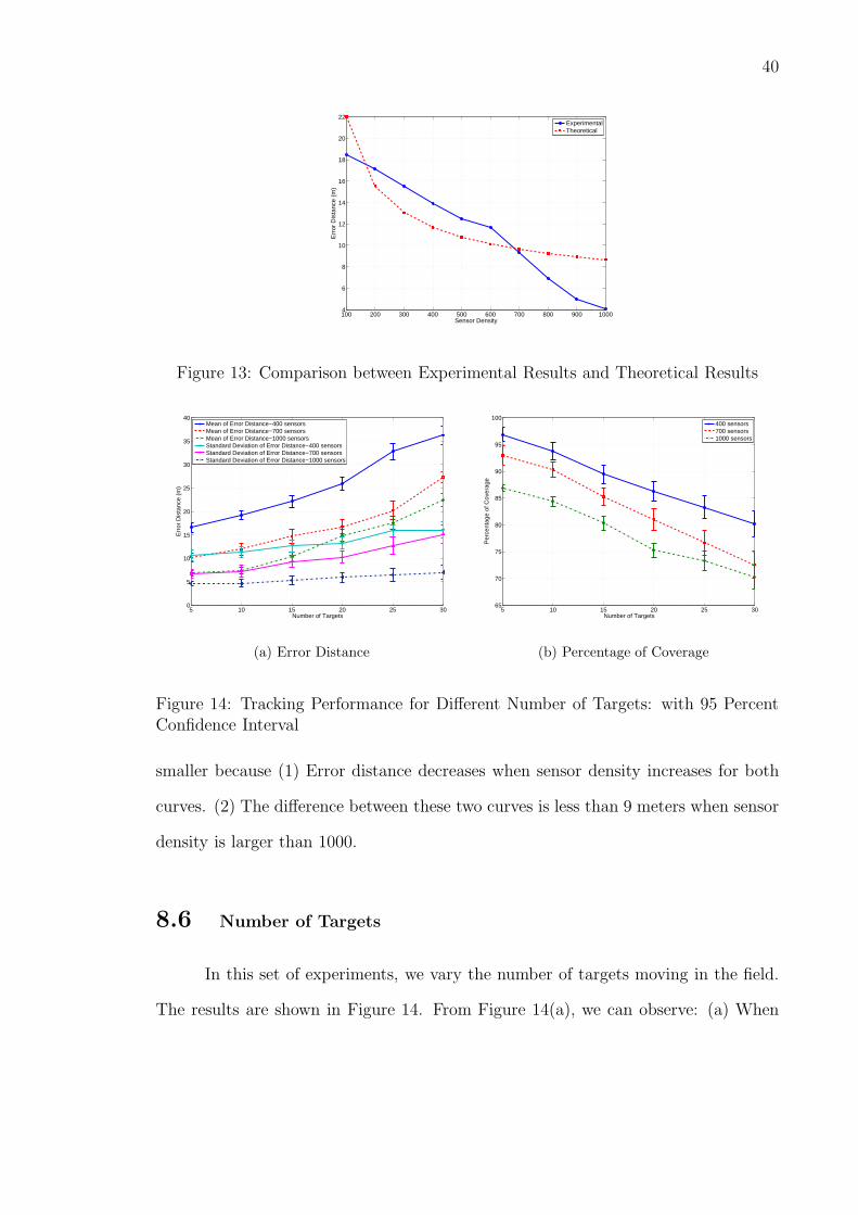
8.6 Number of Targets

In this set of experiments, we vary the number of targets moving in the field.

The results are shown in Figure 14. From Figure 14(a), we can observe: (a) When

41

0.02 0.04 0.06 0.08 0.10 0.125

10

15

20

Speed (m/sample interval)

Err

or D

ista

nce

(m)

Mean of Error DistanceStandard Deviation of Error Distance

Figure 15: Scatter Plot of Tracking Performance vs. Moving Speed

the field is crowded with targets, our algorithm can still track targets with reasonable

accuracy and precision. (b) The error distance increases when the number of targets

increases. It is because the separation step can not perfectly separate out all the

signals when the number of moving targets increases. As shown in Figure 14(b), the

percentage of coverage decreases when the number of targets increases. The decrease

is caused by the decrease in separation performance so that path segments estimated

for different time slots are less consistently covering the actual paths.

8.7 Moving Speed

In this set of experiments, we investigate the effect of the moving speed on

tracking performance. Targets in this set of experiments are moving with different

speed. From experiment results shown in Figure 15, we can observe that the error

distance increases when the moving speed increases. The reasons are as analyzed in

Chapter 6.3: Speed increase can lead to decrease of separation performance and less

number of sensor groups sense enough signal for tracking.

42

100 200 300 400 500 600 700 800 900 10000

5

10

15

20

25

30

Segment Length

Err

or D

ista

nce

(m)

Mean of Error Distance−400sensorsMean of Error Distance−700 sensorsMean of Error Distance−1000 sensorsStandard Deviation of Error Distance−400 sensorsStandard Deviation of Error Distance−700 sensorsStandard Deviation of Error Distance−1000 sensors

100 200 300 400 500 600 700 800 900 100065

70

75

80

85

90

95

100

Segment Length

Per

cent

age

of C

over

age



Figure 16: Effect of Signal Segment Length (lseg) on Tracking Performance: with 95Percent Confidence Interval

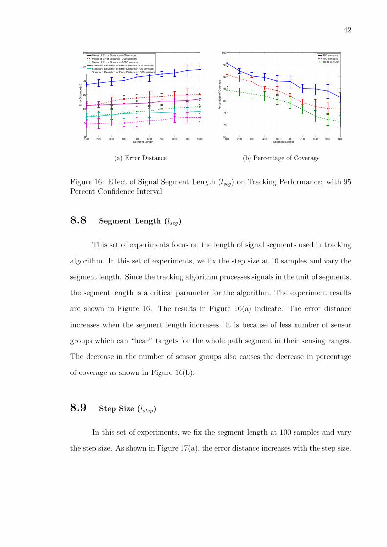
8.8 Segment Length (lseg)

This set of experiments focus on the length of signal segments used in tracking

algorithm. In this set of experiments, we fix the step size at 10 samples and vary the

segment length. Since the tracking algorithm processes signals in the unit of segments,

the segment length is a critical parameter for the algorithm. The experiment results

are shown in Figure 16. The results in Figure 16(a) indicate: The error distance

increases when the segment length increases. It is because of less number of sensor

groups which can “hear” targets for the whole path segment in their sensing ranges.

The decrease in the number of sensor groups also causes the decrease in percentage

of coverage as shown in Figure 16(b).

8.9 Step Size (lstep)

In this set of experiments, we fix the segment length at 100 samples and vary

the step size. As shown in Figure 17(a), the error distance increases with the step size.

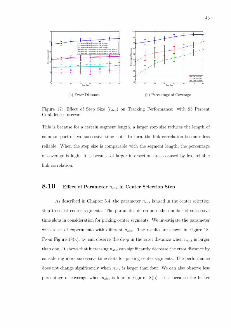
43

10 20 30 40 50 60 70 800

5

10

15

20

25

Step Size

Err

or D

ista

nce

(m)


10 20 30 40 50 60 70 8082

84

86

88

90

92

94

96

98

100

Step Size

Per

cent

age

of C

over

age



Figure 17: Effect of Step Size (lstep) on Tracking Performance: with 95 PercentConfidence Interval

This is because for a certain segment length, a larger step size reduces the length of

common part of two successive time slots. In turn, the link correlation becomes less

reliable. When the step size is comparable with the segment length, the percentage

of coverage is high. It is because of larger intersection areas caused by less reliable

link correlation.

8.10 Effect of Parameter nslot in Center Selection Step

As described in Chapter 5.4, the parameter nslot is used in the center selection

step to select center segments. The parameter determines the number of successive

time slots in consideration for picking center segments. We investigate the parameter

with a set of experiments with different nslot. The results are shown in Figure 18.

From Figure 18(a), we can observe the drop in the error distance when nslot is larger

than one. It shows that increasing nslot can significantly decrease the error distance by

considering more successive time slots for picking center segments. The performance

does not change significantly when nslot is larger than four. We can also observe less

percentage of coverage when nslot is four in Figure 18(b). It is because the better

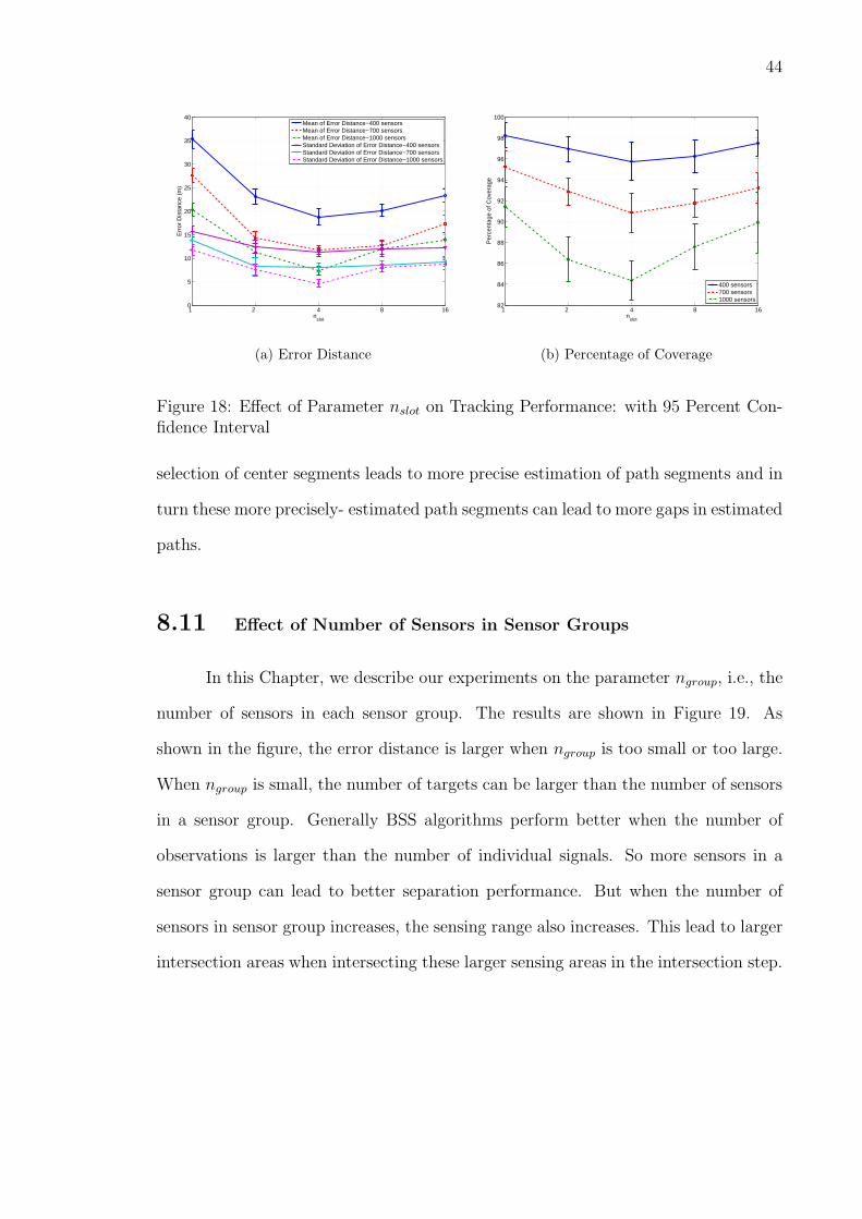
44

1 2 4 8 160

5

10

15

20

25

30

35

40

nslot

Err

or D

ista

nce

(m)


1 2 4 8 1682

84

86

88

90

92

94

96

98

100

nslot

Per

cent

age

of C

over

age



Figure 18: Effect of Parameter nslot on Tracking Performance: with 95 Percent Con-fidence Interval

selection of center segments leads to more precise estimation of path segments and in

turn these more precisely- estimated path segments can lead to more gaps in estimated

paths.

8.11 Effect of Number of Sensors in Sensor Groups

In this Chapter, we describe our experiments on the parameter ngroup, i.e., the

number of sensors in each sensor group. The results are shown in Figure 19. As

shown in the figure, the error distance is larger when ngroup is too small or too large.

When ngroup is small, the number of targets can be larger than the number of sensors

in a sensor group. Generally BSS algorithms perform better when the number of

observations is larger than the number of individual signals. So more sensors in a

sensor group can lead to better separation performance. But when the number of

sensors in sensor group increases, the sensing range also increases. This lead to larger

intersection areas when intersecting these larger sensing areas in the intersection step.

45

5 10 15 20 25 300

5

10

15

20

25

Number of Sensors per Group

Err

or D

ista

nce

(m)


Figure 19: Effect of Number of Sensors in Sensor Groups: with 95 Percent ConfidenceInterval

1 2 4 8 160

5

10

15

20

25

Frequency of Moving Target

Err

or D

ista

nce

(m)


Figure 20: Path with High Frequency Variation: with 95 Percent Confidence Interval

8.12 Paths with High-Frequency Variations

In this set of experiments, we experiment on the performance of tracking targets

following paths with high-frequency variations. In the experiments, we focus on paths

between two points A and B with distance of 300m from each other as shown in Figure

21. Paths between these two points are zigzag paths of different periods. The width

of the path is 100m and we vary zigzag period in our experiments. From the results

shown Figure 20, we can observe the tracking algorithm can track targets following

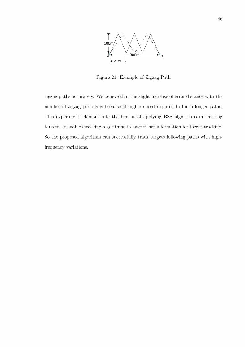
46

300mA

100m

Bperiod

Figure 21: Example of Zigzag Path

zigzag paths accurately. We believe that the slight increase of error distance with the

number of zigzag periods is because of higher speed required to finish longer paths.

This experiments demonstrate the benefit of applying BSS algorithms in tracking

targets. It enables tracking algorithms to have richer information for target-tracking.

So the proposed algorithm can successfully track targets following paths with high-

frequency variations.

CHAPTER IX

TOPOLOGIES OF SENSOR NETWORKS DEPLOYED FOR

TRACKING

9.1 Introduction

In the previous chapters we focus on random topologies of high density sensor

network. In the following chapters we focus on topologies of sensor network to improve

tracking performance. The topology of a sensor network deployed for tracking is

critical to tracking performance: (a) The topology affects separation performance.

For better separation performance, sensors should be clustered so that there are more

sensors than the number of targets within the sensing ranges of these sensors. It is

because BSS algorithms perform better when the number of available mixtures are

larger than the number of source signals. In general better separation performance

leads to better tracking performance. (b) The number of sensors which can “hear” a

target of interest determines how accurate and how precise a tracking algorithm can

estimate the path taken by the target.

We propose cluster-based topologies for better tracking performance. Our

contributions in this Thesis can be summarized as follows:

47

48

∙ We provide a list of necessary requirements on candidate topologies.

∙ We propose cluster-based topologies to improve tracking performance. Guide-

lines of parameter selection for proposed cluster topologies are given in the

Thesis. We evaluate proposed topologies with extensive experiments.

∙ Our empirical experiments show that BSS-based tracking algorithms can achieve

comparable performance in comparison with tracking algorithms assuming ac-

cess to individual signals.

∙ We propose metrics to evaluate performance of proposed topologies using target-

tracking algorithms. The metrics originate from the general metrics used to eval-

uate performance of an estimator in statistics since, essentially, target tracking

algorithms estimate the paths based on data collected from sensor networks.

9.2 System Model and Goal

A general model of tracking targets using wireless sensor networks is shown in

Figure 1.

The goal of this part of the Thesis is to improve tracking performance for

tracking multiple targets with BSS algorithms. We use mean and standard deviation

of error distance to measure tracking performance in this Thesis. The error distance

is defined as the nearest distance between a specific point in the estimated areas to the

actual path taken by a target as shown in Figure 8. The mean and standard deviation

of error distance are calculated based on all the points in estimated areas. The mean

and standard deviation of error distance measures the accuracy and precision of the

tracking algorithm respectively. If we cast the evaluation of the estimation algorithm

in terms of evaluating a statistical estimator, the accuracy corresponds to the bias of

the estimator and the precision corresponds to the variance of the estimator.

49

9.3 Requirements on Candidate Topologies

We focus on topologies of low-density sensor networks simply because the effect

of topologies on tracking performance is negligible for high-density sensor networks.

In this Thesis, we assume that candidate topologies should satisfy the following re-

quirements:

∙ Planned Deployment: The deployment used in tracking targets can be classified

into two categories: random deployment [28] and planned deployment [22, 28].

In random deployment, sensors are distributed randomly over a field. We elimi-

nate random deployment from consideration because for low-density sensor net-

works, the tracking performance of random deployment is usually worse than

the tracking performance of planned deployment.

∙ Full Coverage: In planned deployment, we focus on topologies enabling sensors

to cover the whole field of interest. This requirement is especially important for

low-density sensor networks to prevent targets disappearing from tracking. One

of the reasons to eliminate random deployment from consideration is because

of its possibility of incomplete coverage for low-density sensor networks.

∙ Symmetrical Topology: In this Thesis we only consider symmetrical topologies.

Symmetry is desired because targets can move in various directions and symmet-

rical topologies can ensure that tracking performance is direction-independent.

In this Thesis, we focus on topologies of sensor networks for BSS-based tracking

algorithms: Blind source separation enables tracking algorithms to track multiple

targets based on individual signals instead of aggregate signals. So BSS-based tracking

algorithms can potentially track targets more accurately and precisely and they can

track targets moving along paths of high-frequency variation. We introduce blind

50

source separation and rationale of applying blind source separation to the multiple

target tracking problem below.

CHAPTER X

PROPOSED TOPOLOGIES OF WIRELESS SENSOR NETWORKS

FOR TRACKING

In this Chapter, we introduce topologies proposed for BSS-based tracking al-

gorithms. Before introducing the topologies, we first analyze separation performance

in our experiments and describe rationale behind the proposed topologies.

10.1 Separation Performance

The key step in BSS-based tracking algorithms is to apply BSS algorithms

to recover individual signals from aggregate signals so that tracking algorithms can

have access to individual signals. Obviously the performance of separating out indi-

vidual signals largely dictate overall tracking performance. To investigate the effect

of topologies on separation performance, we did a series of initial experiments with

random topologies.

In these initial experiments, 700 sensors are randomly distributed in a field of

size 1.6km× 1.6km. To remove boundary issues, totally 15 targets are restricted to

move in the field center of size 1km× 1km. Sensing range of each sensor is 250m.

51

52

Table II: Separation Performance vsDcenter

Dcenter(m) Psep

50 - 100 0.4841100 - 150 0.5224150 - 200 0.5301200 - 250 0.5521250 - 300 0.5132

Table III: Separation Performance vsDpair (200m < Dcenter < 250m)

Dpair(m) Psep

50 - 70 0.68170 - 90 0.600590 - 110 0.5152110 - 130 0.4821

A correlation-based metric denoted by Psep is used in our experiments to mea-

sure the separation performance. It is calculated by taking the absolute value of cor-

relation between original signals and separated signals. We use absolute value because

one separated signal may be of different sign in comparison with the corresponding

original signal. The metric Psep is within the range [0, 1]. Two topology-related met-

rics are used in our analysis. We represent the first metric as Dpair. It measures the

average distance between each pair of sensors in a sensor group. The second met-

ric measures the average distance between a target of interest and the center of the

sensor group of interest when the target is moving. We represent the second met-

ric as Dcenter. It is calculated by averaging over 100 data samples. Essentially, the

metric Dpair measures clustering degree of neighboring sensors and the metric Dcenter

measures the distance between a target and a cluster of sensors.

Figure 22 shows the separation performance of these initial experiments. We

present the separation performance visually as a data image in Figure 22, the grid

with the metrics Dpair and Dcenter on x-axis and y-axis respectively. The gray level

of each pixel in the data image represents the separation performance Psep: A darker

pixel indicates better separation performance, i.e., a larger value of Psep.

Table II summarizes separation performance in terms of the distance Dcenter.

From Figure 22 and Table II, we can observe that the separation performance is best

when the distance Dcenter is between 200m and 250m. In other words, the separation

performance is best when the target is away from one sensor group and still within

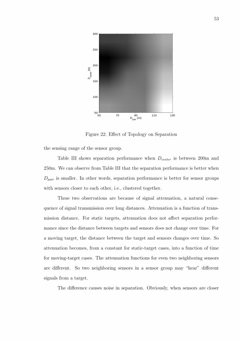
53

Dpair

(m)

Dce

nter

(m)

50 70 90 110 130

300

250

200

150

100

50

Figure 22: Effect of Topology on Separation

the sensing range of the sensor group.

Table III shows separation performance when Dcenter is between 200m and

250m. We can observe from Table III that the separation performance is better when

Dpair is smaller. In other words, separation performance is better for sensor groups

with sensors closer to each other, i.e., clustered together.

These two observations are because of signal attenuation, a natural conse-

quence of signal transmission over long distances. Attenuation is a function of trans-

mission distance. For static targets, attenuation does not affect separation perfor-

mance since the distance between targets and sensors does not change over time. For

a moving target, the distance between the target and sensors changes over time. So

attenuation becomes, from a constant for static-target cases, into a function of time

for moving-target cases. The attenuation functions for even two neighboring sensors

are different. So two neighboring sensors in a sensor group may “hear” different

signals from a target.

The difference causes noise in separation. Obviously, when sensors are closer

54d interd intraSensor Cluster centerFigure 23: Example of Cluster Topology

to each other and the target of interest is away from these sensors, the difference in

attenuation functions of these sensors is smaller. In turn, less noise is generated in

separation and better separation performance can be achieved.

10.2 Proposed Topologies

Based on observations made in our initial experiments, we propose cluster

topologies for BSS-based tracking algorithms as shown Figure 23:

In the proposed topologies, sensors are placed into clusters and sensor clusters

are distributed evenly in a field. The proposed cluster topologies have four parame-

ters:

∙ In-cluster arrangement: Within each cluster, sensors are arranged in regular

patterns. The possible choices are any polygon-based patterns such as well-

known triangle lattice pattern, square pattern, pentagon pattern, and hexagon

pattern. Our experiments indicate that tracking performance is not sensitive to

55

patterns for in-cluster arrangement. So, we choose square pattern in this Thesis

since research results on data segmentation [44], routing [19], and storage [10]

recommend the square pattern. For the same reason, we arrange clusters in a

field in square pattern.

∙ Number of sensors per cluster nclst: This parameter specifies the number of sen-

sors within each sensor cluster. For better separation performance, the number

of sensors per cluster should be no less than the number of targets moving in

the sensing range of a cluster. Potentially all the targets can move into the

sensing range of one cluster, so we set the number of sensors per cluster close

to the number of targets in the field.

∙ Inter-cluster distance dinter: As shown in Figure 23, the inter-cluster distance is

the distance between two centers of neighboring sensor clusters. This parameter

depends on N , the total number of sensors to be deployed in the field, and nclst,

the number of sensors per cluster.

∙ Intra-cluster distance dintra: Intra-cluster distance is the distance between the

center of a sensor cluster and the furthest sensor within the same cluster. It is

a measure of clustering degree. To avoid the merge of neighboring clusters, the

parameter dintra should be less than dinter

2. Our initial experiments shown in

Figure 22 indicate that better separation performance is achieved where sensors

are close to each other. But it is not desired to cluster sensors in a very small

area because (a) It may leave lots of uncovered spots in the field when sensor

density is low. (b) When sensors are too close to each other, sensors “hear”

roughly the same mixture of individual signals. In this case the separation

performance can not be good. So we suggest dintra to be close to dinter

4. Our

further experiments also support the choice of the parameter.

56

Besides considerations on separation performance, we propose cluster topolo-

gies because they satisfy the requirements listed in chapter 9.3: It is symmetric and

it can cover the whole field. The proposed cluster topology is general: Grid topology

is a special case of the cluster topology when nclst = 1.

CHAPTER XI

PERFORMANCE EVALUATION OF PROPOSED TOPOLOGIES

We evaluate the performance of tracking algorithm in our proposed topology

with extensive simulations with Matlab. We assume acoustic sensors are deployed in

the field of interest for tracking purpose.

11.1 Experiment Setup

In the following experiments, the simulated field is a 1.6km × 1.6km square

area. The movement of targets is restricted to a 1km × 1km center area to eliminate

boundary effects. The signals used for tracking are real bird signals downloaded from

the website of Florida Museum of Natural History [21]. The attenuation of sound

signals is according to atmospheric sound absorption model [30]. We choose low-

density sensor network with density N =128 and 288 sensors. The sensing range of

sensors is 250m. In the following experiments, targets are moving at a speed below

0.15 meter per sample interval. The performance metrics used in our experiments is

mean and standard deviation of error distance. In all the following experiments we

compare our cluster topology with grid and random topologies.

57

58

11.2 Number of Sensors per Cluster (nclust)

In this set of experiments, we vary the number of sensors per cluster nclust. We

choose dintra=80m according to parameter selection guidelines in chapter 10.2. The

inter-cluster distance depends on the sensor density N and the number of sensors

per cluster nclust. For N=128, the inter-cluster distance dinter=320m and 533.33m for

nclust =8 and 32 respectively. And forN=288, the inter-cluster distance dinter=228.57m

and 400m for nclust =8 and 32 respectively. The number of moving targets ntargets is

10 or 30 in this set of experiments. As shown in Figure 24, for the experiments on 128

sensors (N=128), the minimum error distance is achieved for 10 targets (ntargets=10)

when nclust=8. In the same experiments, the best tracking performance for 30 targets

is achieved when nclust=32. These experiment results indicate the number of sensors

per cluster nclust should be close to the number of targets as suggested in parame-

ter selection guidelines given in Section 10.2. In comparison with grid and random

topologies, performance increase for the cluster topology is 18.75% and 23.28% for

10 and 30 moving targets respectively when N=128. For 288 sensors (N=288), the

increase is 26.12% and 27.90% for 10 and 30 moving targets respectively. We can

also observe that performance of the cluster topology with selected parameters can

be 33.62% and 32.78% better than random and grid topologies respectively.

11.3 Effect of In-Cluster Arrangement

In this set of experiments, we investigate the effect of in-cluster topologies. We

experiment on the square pattern and the pentagon pattern as in-cluster arrangement.

Similar experiment results are got from other polygons. Parameters used in this set

of experiments are dintra=80m and ntargets =10. As shown in Figure 25(a) and 25(b),

we observe that tracking performance is not sensitive to in-cluster arrangement.

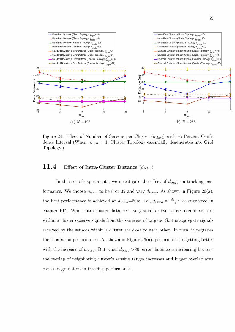
59

1 2 8 32 12110

15

20

25

30

35

40

nclust

Err

or

Dis

tance (

m)

Mean Error Distance (Cluster Topology, ntargets

=10)


=30)

Mean Error Distance (Random Topology, ntargets

=10)


=30)

Standard Deviation of Error Distance (Cluster Topology, ntargets

=10)


=30)

Standard Deviation of Error Distance (Random Topology, ntargets

=10)

Standard Deviation of Error Distance (Random topology, ntargets

=30)

1 2 8 32 725

10

15

20

25

30

35

nclust

Err

or

Dis

tance (

m)


=10)


=30)


=10)


=30)


=10)


=30)


=10)


=30)

(a) N =128 (b) N =288

Figure 24: Effect of Number of Sensors per Cluster (nclust) with 95 Percent Confi-dence Interval (When nclust = 1, Cluster Topology essentially degenerates into GridTopology.)

11.4 Effect of Intra-Cluster Distance (dintra)

In this set of experiments, we investigate the effect of dintra on tracking per-

formance. We choose nclust to be 8 or 32 and vary dintra. As shown in Figure 26(a),

the best performance is achieved at dintra=80m, i.e., dintra ≈ dintra

4as suggested in

chapter 10.2. When intra-cluster distance is very small or even close to zero, sensors

within a cluster observe signals from the same set of targets. So the aggregate signals

received by the sensors within a cluster are close to each other. In turn, it degrades

the separation performance. As shown in Figure 26(a), performance is getting better

with the increase of dintra. But when dintra >80, error distance is increasing because

the overlap of neighboring cluster’s sensing ranges increases and bigger overlap area

causes degradation in tracking performance.

60

8 32 1210

5

10

15

20

25

30

35

nclust

Mea

n E

rror

Dis

tanc

e (m

)

Square PatternPentagon Pattern

8 32 720

5

10

15

20

25

30

nclust

Mea

n E

rror

Dis

tanc

e (in

m)

Square PatternPentagon Pattern

(a) Error Distance of N=128 (b) Error Distance of N=288

Figure 25: Effect of In-Cluster Arrangement on Tracking Performance

11.5 Effect of Number of Targets (ntargets)

In this set of experiments, we investigate the effect of number of targets on

tracking performance. Table VII shows the typical performance increase of cluster

topology over grid and random topologies. The experiment parameters are as follows:

density N =288, nclust =32, and dintra =80m. Table IV, V, VI, VII shows percent-

age of increase in performance of cluster topology over grid and random topologies

over different experiment settings. We can observe that percentage of increase can

achieve 37.18% and 35.02% for 40 targets over random topologies and grid topologies

respectively. Table VII shows that performance increase becomes larger when the

number of targets increases. It is mainly because better separation performance can

be achieved for cluster topology.

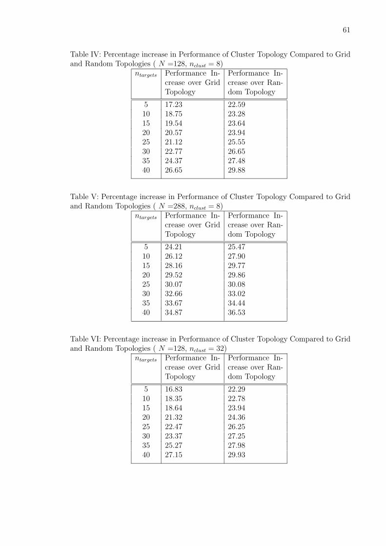
61

Table IV: Percentage increase in Performance of Cluster Topology Compared to Gridand Random Topologies ( N =128, nclust = 8)

ntargets Performance In-crease over GridTopology

Performance In-crease over Ran-dom Topology

5 17.23 22.5910 18.75 23.2815 19.54 23.6420 20.57 23.9425 21.12 25.5530 22.77 26.6535 24.37 27.4840 26.65 29.88

Table V: Percentage increase in Performance of Cluster Topology Compared to Gridand Random Topologies ( N =288, nclust = 8)



5 24.21 25.4710 26.12 27.9015 28.16 29.7720 29.52 29.8625 30.07 30.0830 32.66 33.0235 33.67 34.4440 34.87 36.53

Table VI: Percentage increase in Performance of Cluster Topology Compared to Gridand Random Topologies ( N =128, nclust = 32)



5 16.83 22.2910 18.35 22.7815 18.64 23.9420 21.32 24.3625 22.47 26.2530 23.37 27.2535 25.27 27.9840 27.15 29.93

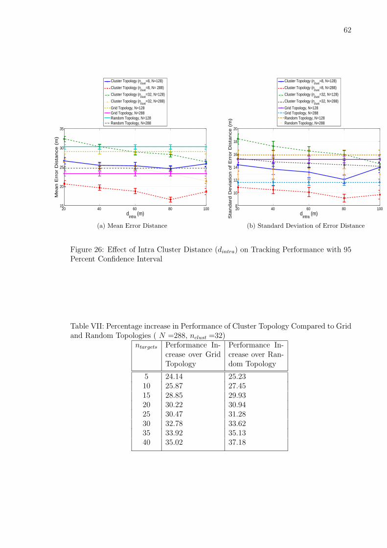
62

20 40 60 80 10015

20

25

30

35

dintra

(m)

Mean E

rror

Dis

tance (

m)

Cluster Topology (nclust

=8, N=128)


=8, N= 288)


=32, N=128)


=32, N=288)

Grid Topology, N=128Grid Topology, N=288Random Topology, N=128 Random Topology, N=288

20 40 60 80 1008

10

12

14

16

18

20

dintra

(m)

Sta

ndard

Devia

tion o

f E

rror

Dis

tance (

m)


=8, N=128)


=8, N=288)


=32, N=128)


=32, N=288)

Grid Topology, N=128 Grid Topology, N=288 Random Topology, N=128 Random Topology, N=288

(a) Mean Error Distance (b) Standard Deviation of Error Distance

Figure 26: Effect of Intra Cluster Distance (dintra) on Tracking Performance with 95Percent Confidence Interval

Table VII: Percentage increase in Performance of Cluster Topology Compared to Gridand Random Topologies ( N =288, nclust =32)



5 24.14 25.2310 25.87 27.4515 28.85 29.9320 30.22 30.9425 30.47 31.2830 32.78 33.6235 33.92 35.1340 35.02 37.18

CHAPTER XII

DISCUSSION

The complexity of the algorithm is largely determined by the step size shown

in Figure 3. The number of separations performed by the algorithm is in the order

of O( Llstep× Ngrps), where L is the total number of samples in one aggregate signal,

lstep is the step size and Ngrps is the number of sensor groups. A larger step size can

reduce the number of separations performed by the algorithm. The cost will be slight

degradation of tracking performance as shown in Figure 17(a).

In this Thesis, we assume the sensors are placed randomly in the field. From the

analysis in Chapter 6, we know that better separation performance can be achieved

when sensor groups are distant from targets and sense targets. So we can possibly

reduce the number of sensors needed for tracking by placed sensors in a better way

such as in clusters. This is one of the topics in our future work.

In this Thesis, we use BSS algorithms for the tracking purpose. The algorithms

can also be used to process data collected by sensor networks for other applications.

Since data collected by sensors is essentially aggregate data and BSS algorithms can

recover data generated by different sources from aggregate data, analysis based on

BSS algorithms can be more accurate.

63

CHAPTER XIII

CONCLUSION

We propose a general approach to track multiple targets using wireless sensor

networks. The approach is based on blind source separation (BSS) algorithms. By

applying BSS algorithms on aggregate signals collected from sensors, we can recover

individual signals from targets for tracking. The proposed tracking algorithm fully

utilize both spatial and temporal information available for tracking. We evaluate

the proposed tracking algorithm both experimentally and theoretically. The tracking

algorithm can track targets both accurately and precisely. Because of richer infor-

mation made available by BSS algorithms, the proposed algorithm can also track

paths with high-frequency variations. And also we propose cluster topologies to im-

prove tracking performance of BSS-based tracking algorithms. A set of guidelines

on parameter selection for proposed topologies are given in the Thesis. We evaluate

proposed topologies with extensive experiments. The proposed topology can achieve

more than 35 percent improvement in tracking performance over grid and random

topologies. Our empirical experiments show that BSS-based tracking algorithm can

achieve comparable tracking performance in comparison with algorithms assuming

access to individual signals.

64

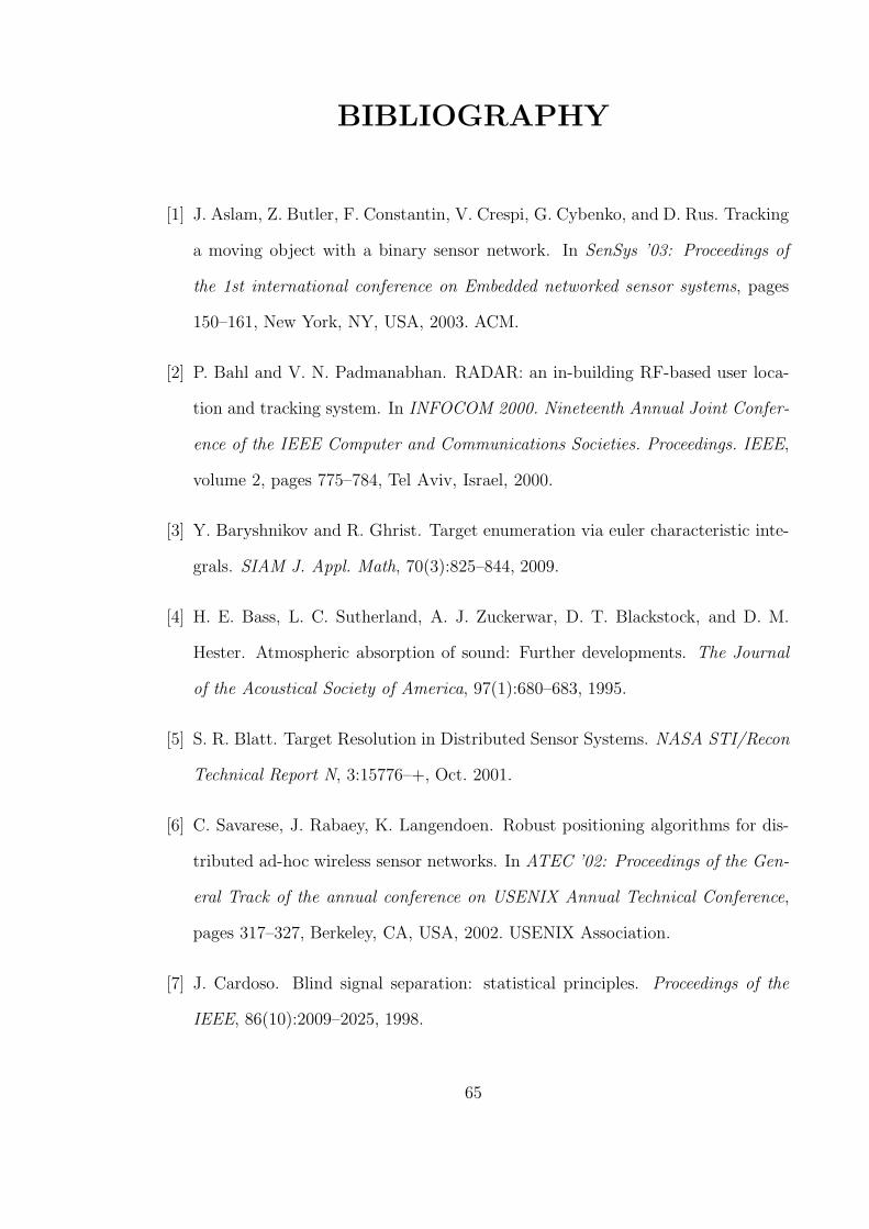
BIBLIOGRAPHY

[1] J. Aslam, Z. Butler, F. Constantin, V. Crespi, G. Cybenko, and D. Rus. Tracking

a moving object with a binary sensor network. In SenSys ’03: Proceedings of

the 1st international conference on Embedded networked sensor systems, pages

150–161, New York, NY, USA, 2003. ACM.

[2] P. Bahl and V. N. Padmanabhan. RADAR: an in-building RF-based user loca-

tion and tracking system. In INFOCOM 2000. Nineteenth Annual Joint Confer-

ence of the IEEE Computer and Communications Societies. Proceedings. IEEE,

volume 2, pages 775–784, Tel Aviv, Israel, 2000.

[3] Y. Baryshnikov and R. Ghrist. Target enumeration via euler characteristic inte-

grals. SIAM J. Appl. Math, 70(3):825–844, 2009.

[4] H. E. Bass, L. C. Sutherland, A. J. Zuckerwar, D. T. Blackstock, and D. M.

Hester. Atmospheric absorption of sound: Further developments. The Journal

of the Acoustical Society of America, 97(1):680–683, 1995.

[5] S. R. Blatt. Target Resolution in Distributed Sensor Systems. NASA STI/Recon

Technical Report N, 3:15776–+, Oct. 2001.

[6] C. Savarese, J. Rabaey, K. Langendoen. Robust positioning algorithms for dis-

tributed ad-hoc wireless sensor networks. In ATEC ’02: Proceedings of the Gen-

eral Track of the annual conference on USENIX Annual Technical Conference,

pages 317–327, Berkeley, CA, USA, 2002. USENIX Association.

[7] J. Cardoso. Blind signal separation: statistical principles. Proceedings of the

IEEE, 86(10):2009–2025, 1998.

65

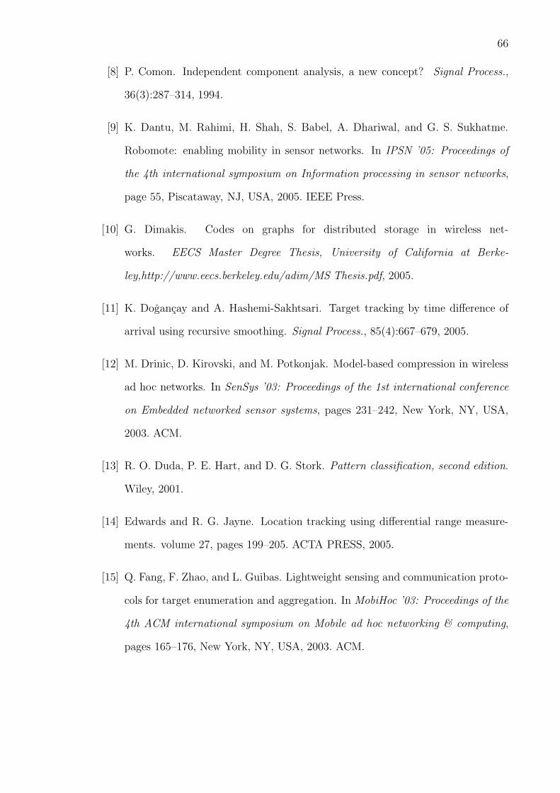
66

[8] P. Comon. Independent component analysis, a new concept? Signal Process.,

36(3):287–314, 1994.

[9] K. Dantu, M. Rahimi, H. Shah, S. Babel, A. Dhariwal, and G. S. Sukhatme.

Robomote: enabling mobility in sensor networks. In IPSN ’05: Proceedings of

the 4th international symposium on Information processing in sensor networks,

page 55, Piscataway, NJ, USA, 2005. IEEE Press.

[10] G. Dimakis. Codes on graphs for distributed storage in wireless net-

works. EECS Master Degree Thesis, University of California at Berke-

ley,http://www.eecs.berkeley.edu/adim/MS Thesis.pdf, 2005.

[11] K. Dogancay and A. Hashemi-Sakhtsari. Target tracking by time difference of

arrival using recursive smoothing. Signal Process., 85(4):667–679, 2005.

[12] M. Drinic, D. Kirovski, and M. Potkonjak. Model-based compression in wireless

ad hoc networks. In SenSys ’03: Proceedings of the 1st international conference

on Embedded networked sensor systems, pages 231–242, New York, NY, USA,

2003. ACM.

[13] R. O. Duda, P. E. Hart, and D. G. Stork. Pattern classification, second edition.

Wiley, 2001.

[14] Edwards and R. G. Jayne. Location tracking using differential range measure-

ments. volume 27, pages 199–205. ACTA PRESS, 2005.

[15] Q. Fang, F. Zhao, and L. Guibas. Lightweight sensing and communication proto-

cols for target enumeration and aggregation. In MobiHoc ’03: Proceedings of the

4th ACM international symposium on Mobile ad hoc networking & computing,

pages 165–176, New York, NY, USA, 2003. ACM.

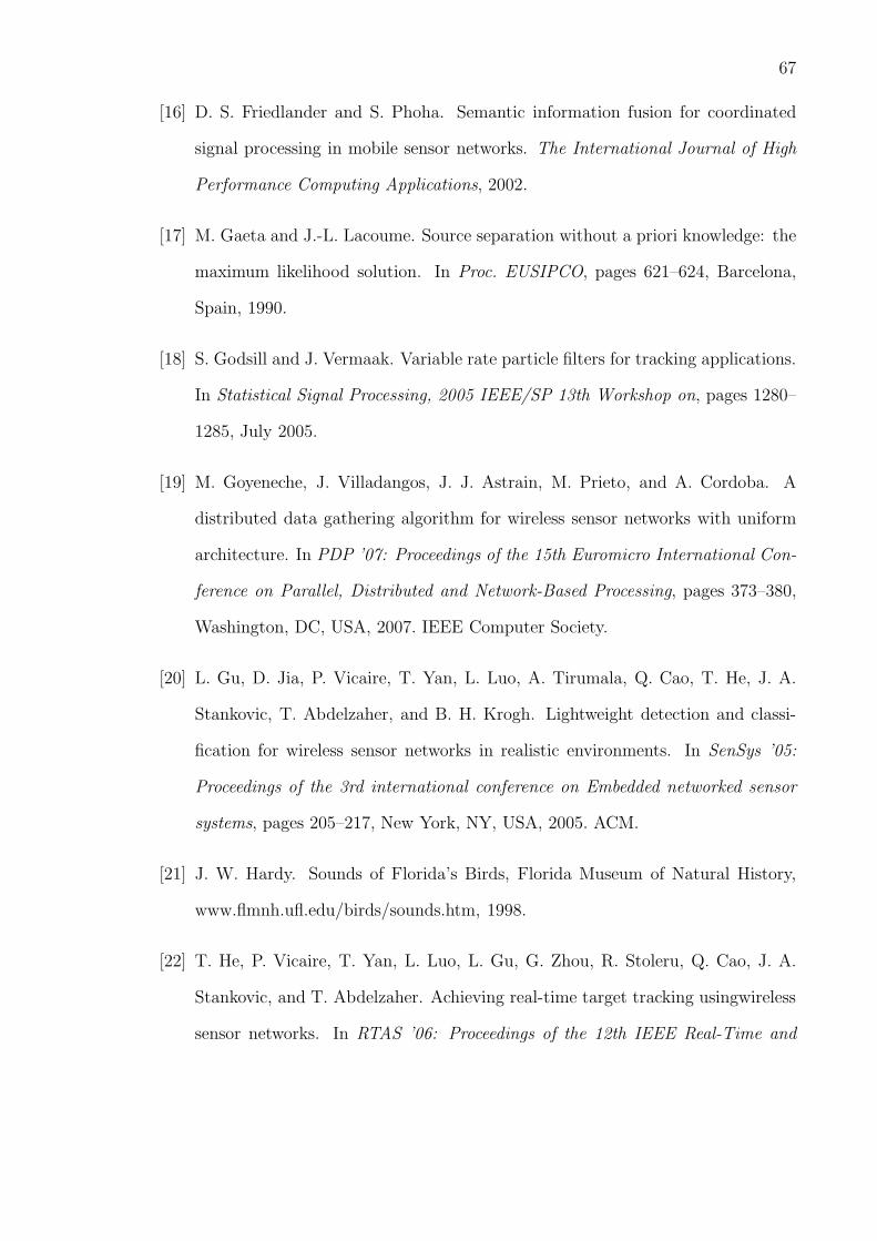
67

[16] D. S. Friedlander and S. Phoha. Semantic information fusion for coordinated

signal processing in mobile sensor networks. The International Journal of High

Performance Computing Applications, 2002.

[17] M. Gaeta and J.-L. Lacoume. Source separation without a priori knowledge: the

maximum likelihood solution. In Proc. EUSIPCO, pages 621–624, Barcelona,

Spain, 1990.

[18] S. Godsill and J. Vermaak. Variable rate particle filters for tracking applications.

In Statistical Signal Processing, 2005 IEEE/SP 13th Workshop on, pages 1280–

1285, July 2005.

[19] M. Goyeneche, J. Villadangos, J. J. Astrain, M. Prieto, and A. Cordoba. A

distributed data gathering algorithm for wireless sensor networks with uniform

architecture. In PDP ’07: Proceedings of the 15th Euromicro International Con-

ference on Parallel, Distributed and Network-Based Processing, pages 373–380,

Washington, DC, USA, 2007. IEEE Computer Society.

[20] L. Gu, D. Jia, P. Vicaire, T. Yan, L. Luo, A. Tirumala, Q. Cao, T. He, J. A.

Stankovic, T. Abdelzaher, and B. H. Krogh. Lightweight detection and classi-

fication for wireless sensor networks in realistic environments. In SenSys ’05:

Proceedings of the 3rd international conference on Embedded networked sensor

systems, pages 205–217, New York, NY, USA, 2005. ACM.

[21] J. W. Hardy. Sounds of Florida’s Birds, Florida Museum of Natural History,

www.flmnh.ufl.edu/birds/sounds.htm, 1998.

[22] T. He, P. Vicaire, T. Yan, L. Luo, L. Gu, G. Zhou, R. Stoleru, Q. Cao, J. A.

Stankovic, and T. Abdelzaher. Achieving real-time target tracking usingwireless

sensor networks. In RTAS ’06: Proceedings of the 12th IEEE Real-Time and

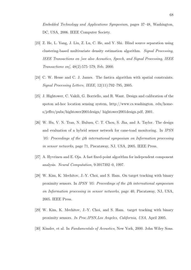
68

Embedded Technology and Applications Symposium, pages 37–48, Washington,

DC, USA, 2006. IEEE Computer Society.

[23] Z. He, L. Yang, J. Liu, Z. Lu, C. He, and Y. Shi. Blind source separation using

clustering-based multivariate density estimation algorithm. Signal Processing,

IEEE Transactions on [see also Acoustics, Speech, and Signal Processing, IEEE

Transactions on], 48(2):575–579, Feb. 2000.

[24] C. W. Hesse and C. J. James. The fastica algorithm with spatial constraints.

Signal Processing Letters, IEEE, 12(11):792–795, 2005.

[25] J. Hightower, C. Vakili, G. Borriello, and R. Want. Design and calibration of the

spoton ad-hoc location sensing system, http://www.cs.washington. edu/home-

s/jeffro/pubs/hightower2001design/ hightower2001design.pdf, 2001.

[26] W. Hu, V. N. Tran, N. Bulusu, C. T. Chou, S. Jha, and A. Taylor. The design

and evaluation of a hybrid sensor network for cane-toad monitoring. In IPSN

’05: Proceedings of the 4th international symposium on Information processing

in sensor networks, page 71, Piscataway, NJ, USA, 2005. IEEE Press.

[27] A. Hyvrinen and E. Oja. A fast fixed-point algorithm for independent component

analysis. Neural Computation, 9:3917392–0, 1997.

[28] W. Kim, K. Mechitov, J.-Y. Choi, and S. Ham. On target tracking with binary

proximity sensors. In IPSN ’05: Proceedings of the 4th international symposium

on Information processing in sensor networks, page 40, Piscataway, NJ, USA,

2005. IEEE Press.

[29] W. Kim, K. Mechitov, J.-Y. Choi, and S. Ham. target tracking with binary

proximity sensors. In Proc.IPSN,Los Angeles, California, USA, April 2005.

[30] Kinsler, et al. In Fundamentals of Acoustics, New York, 2000. John Wiley Sons.

69

[31] C. Kreucher, K. Kastella, and I. Hero, A.O. Multitarget tracking using the

joint multitarget probability density. Aerospace and Electronic Systems, IEEE

Transactions on, 41(4):1396–1414, Oct. 2005.

[32] B. Kusy and J. Sallai. CRAWDAD data set vander-

bilt/interferometric (v. 2007-06-06). Downloaded from

http://crawdad.cs.dartmouth.edu/vanderbilt/interferometric, June 2007.

[33] B. Kusy, J. Sallai, G. Balogh, A. Ledeczi, V. Protopopescu, J. Tolliver, F. DeNap,

and M. Parang. Radio interferometric tracking of mobile wireless nodes. In

MobiSys ’07: Proceedings of the 5th international conference on Mobile systems,

applications and services, pages 139–151, New York, NY, USA, 2007. ACM.

[34] S.-P. K. Y.-C. T. F.-J. W. C.-Y. Lin. A probabilistic signal-strength-based

evaluation methodology for sensor network deployment. Advanced Information

Networking and Applications, 2005. AINA 2005. 19th International Conference,

1:Taipei, Taiwan, 319 – 324, March 2005.

[35] J. Liu, M. Chu, and J. Reich. Multitarget tracking in distributed sensor networks.

Signal Processing Magazine, IEEE, 24(3):36–46, May 2007.

[36] R. F. Lutomirski and R. G. Buser. Phase difference and angle-of-arrival fluctu-

ations in tracking a moving point source. Appl. Opt., 13(12):2869, 1974.

[37] D. Macagnano, G. Destino, F. Esposito, and G. Abreu. Mac performances for

localization and tracking in wireless sensor networks. In Positioning, Navigation

and Communication, 2007. WPNC apos;07., volume 22, pages 297 – 302, March

2007.

[38] B. Malhotra and A. Aravind. Path-adaptive on-site tracking in wireless sensor

networks. IEICE - Trans. Inf. Syst., E89-D(2):536–545, 2006.

70

[39] M. Moghavvemi and L. C. Seng. Pyroelectric infrared sensor for intruder de-

tection. In TENCON 2004. 2004 IEEE Region 10 Conference, pages 656–659,

Chiang Mai, Thailand, Nov. 2004.

[40] M. Morelande, C. Kreucher, and K. Kastella. A bayesian approach to multi-

ple target detection and tracking. Signal Processing, IEEE Transactions on,

55(5):1589–1604, May 2007.

[41] A. Nasipuri and K. Li. A directionality based location discovery scheme for

wireless sensor networks. In WSNA ’02: Proceedings of the 1st ACM interna-

tional workshop on Wireless sensor networks and applications, pages 105–111,

New York, NY, USA, 2002. ACM.

[42] E. Olson, J. J. Leonard, and S. Teller. Robust range-only beacon localization.

Oceanic Engineering, IEEE Journal of, 31(4):949–958, Oct. 2006.

[43] Q. Pan, J. Wei, H. Cao, N. Li, and H. Liu. Improved ds acoustic-seismic modality

fusion for ground-moving target classification in wireless sensor networks. Pattern

Recogn. Lett., 28(16):2419–2426, 2007.

[44] A. Panangadan and G. Sukhatme. Data segmentation for region detection

in a sensor network. CRES Technical Report 05-005, University of Southern

California,http://cres.usc.edu/cgi-bin/print pub details.pl?pubid=434, 2005.

[45] A. Pereira, A. Monteiro, L. Nunes, and N. Costa. Wireless sensor network for mo-

bile entities localization people monitor. In ICSNC ’07: Proceedings of the Second

International Conference on Systems and Networks Communications, page 51,

Washington, DC, USA, 2007. IEEE Computer Society.

[46] D. Pham and P. Garrat. Blind separation of mixture of inde-

71

pendent sources through a quasi-maximum likelihood approach, cite-

seer.ist.psu.edu/pham97blind.html, 1997.

[47] K. Pister, J. Kahn, and B. Boser. Smartdust: wireless networks of millimeter-

scale sensor nodes, 1999.

[48] N. B. Priyantha, A. Chakraborty, and H. Balakrishnan. The cricket location-

support system. In MobiCom ’00: Proceedings of the 6th annual international

conference on Mobile computing and networking, pages 32–43, New York, NY,

USA, 2000. ACM Press.

[49] S. Ray, W. Lai, and I. C. Paschalidis. Statistical location detection with sensor

networks. IEEE/ACM Trans. Netw., 14(SI):2670–2683, 2006.

[50] S. Ray, D. Starobinski, A. Trachtenberg, and R. Ungrangsi. Robust location

detection with sensor networks. IEEE Journal on Selected Areas in Communi-

cations, 22(6):1016–1025, 2004.

[51] N. Shrivastava, R. M. U. Madhow, and S. Suri. Target tracking with binary

proximity sensors: fundamental limits, minimal descriptions, and algorithms.

In SenSys ’06: Proceedings of the 4th international conference on Embedded

networked sensor systems, pages 251–264, New York, NY, USA, 2006. ACM.

[52] J. Singh, U. Madhow, R. Kumar, S. Suri, and R. Cagley. Tracking multiple

targets using binary proximity sensors. In IPSN ’07: Proceedings of the 6th

international conference on Information processing in sensor networks, pages

529–538, New York, NY, USA, 2007. ACM.

[53] L. D. Stone, T. L. Corwin, and C. A. Barlow. Bayesian Multiple Target Tracking.

Artech House, Inc., Norwood, MA, USA, 1999.

72

[54] C. Tang and C. Raghavendra. Compression techniques for wireless sensor net-

works. pages 207–231. 2004.

[55] L. Tong, Y. Inouye, and R. Liu. Waveform-preserving blind estimation of multi-

ple independent sources. IEEE Transactions on Signal Processing, 41(7):2461–

2470, July 1993.

[56] L. Tong, V. Soon, and Y. F. H. R. Liu. Indeterminacy and identifiability of blind

identification. IEEE Transactions, 38:499–509, March 1991.

[57] J. Vermaak, S. Godsill, and P. Perez. Monte carlo filtering for multi target track-

ing and data association. Aerospace and Electronic Systems, IEEE Transactions

on, 41(1):309–332, Jan. 2005.

[58] B. Vo, N. Ma, P. Ching, and K. Wong. Tracking moving speech source using

cyclic adaptive beamforming. Electronics Letters, 36(19):1666–1668, Sep 2000.

[59] P. von Rickenbach and R. Wattenhofer. Gathering correlated data in sensor

networks. In DIALM-POMC ’04: Proceedings of the 2004 joint workshop on

Foundations of mobile computing, pages 60–66, New York, NY, USA, 2004. ACM.

[60] S. Yang, Y. Kim, and H. Choi. Vehicle identification using wireless sensor net-

works. In Proceedings. IEEE, Richmond, VA,, pages 41 – 46, March 2007.

[61] B. Zaidi, Z.R. Mark. A mobility tracking model for wireless ad hoc networks.

In Wireless Communications and Networking, 2003. WCNC 2003. 2003 IEEE,

volume 3, pages 1790– 1795, New Orleans, LA, USA, March 2003.

[62] G. V. Zaruba, M. Huber, F. A. Kamangar, and I. Chlamtac. Indoor location

tracking using rssi readings from a single wi-fi access point. volume 13, pages

221–235, Hingham, MA, USA, 2007. Kluwer Academic Publishers.

73

APPENDIX

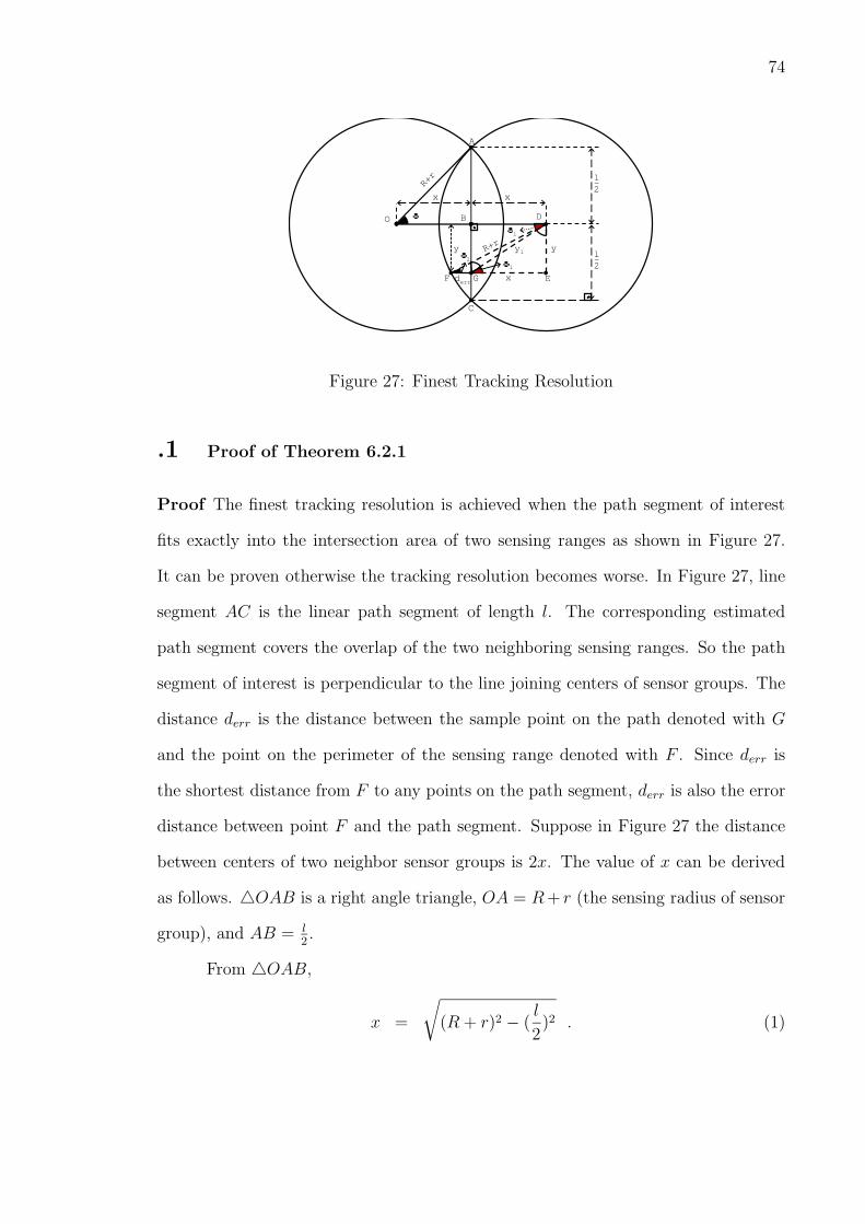
74

derr

R+r

R+r

O

A

EGF

DB

x

y

x

y1

x

yl-2

l-2θ

C

θ2 θ

1

θ1

Figure 27: Finest Tracking Resolution

.1 Proof of Theorem 6.2.1

Proof The finest tracking resolution is achieved when the path segment of interest

fits exactly into the intersection area of two sensing ranges as shown in Figure 27.

It can be proven otherwise the tracking resolution becomes worse. In Figure 27, line

segment AC is the linear path segment of length l. The corresponding estimated

path segment covers the overlap of the two neighboring sensing ranges. So the path

segment of interest is perpendicular to the line joining centers of sensor groups. The

distance derr is the distance between the sample point on the path denoted with G

and the point on the perimeter of the sensing range denoted with F . Since derr is

the shortest distance from F to any points on the path segment, derr is also the error

distance between point F and the path segment. Suppose in Figure 27 the distance

between centers of two neighbor sensor groups is 2x. The value of x can be derived

as follows. △OAB is a right angle triangle, OA = R+ r (the sensing radius of sensor

group), and AB = l2.

From △OAB,

x =

√

(R + r)2 − (l

2)2 . (1)

75

Thus the distance between neighbor sensor groups is 2x, i.e., 2√

(R + r)2 − ( l2)2.

The error distance derr can be derived as follows: From △DGE as shown in Figure

27,

tan�1 =y

x,

�1 = tan−1 y

x, (2)

x =y

tan�1. (3)

Now from △FDE, FD = R+ r (the sensing radius of sensor group). We denote the

distance between the point B and G with y. From △FDE,

�2 = sin−1(y

R + r) , (4)

and

tan�2 =y

derr + x,

derr =y

tan�2− x ,

(5)

where x is from Equation 3 and �2 is from Equation 4. Since

derr =y

tan�2− y

tan�1, (6)

we can further simplify the above equation by substituting �1 and �2 values derived

in Equation 2 and Equation 4 respectively. So derr can be derived as follows:

derr = (R + r) cos(�2)−√

(R + r)2 − (l

2)2 . (7)

For all the points on the line segment FG, the average error distance is derr2. Integral

is used to calculate average of error distance for all the points within the intersection

76

area. Thus the finest tracking resolution is 12

l/2∫

0

{ (R+r)cos(�2)−√

(R+r)2−( l2)2

l}dy where

�2 = sin−1( yR+r

).

After further simplification the finest tracking resolution becomes (R+r)2

4lsin−1( l

2(R+r))−

18

√

(R + r)2 − ( l2)2.

77

.2 Proof of Theorem 6.2.3

A

O DB

x x

l-2

l-2θ

C

R+ry

F

θ1

derr EG

y1 y

x

θ2

θ1

Figure 28: Average Tracking Resolution

Proof From △FDE as shown in Figure 28,

cos�2 =y

R + r,

�2 = cos−1(y

R + r) . (8)

We derived the error distance derr in Appendix .1.

derr =y

tan�2− y

tan�1, (9)

we can further simplify the above Equation by substituting �1 and �2 values derived

in Equation 2 and Equation 8 respectively. Then derr can be derived as follows:

derr = (R + r) cos �2 − x , (10)

where �2 = sin−1( yr+R

). So the mean error distance is 12

l/2∫

0

{(R+ r)cos�2 − x}dy.

From Corollary 6.2.2, we know the distance between the centers of two sen-

sor groups when the finest tracking resolution is achieved. The worst-case tracking

resolution is achieved when the distance between the centers of two sensor groups is

78

R + r. The average tracking resolution can be derived by integral of mean error dis-

tance over possible distance between the centers of two sensor groups. So the average

tracking resolution is 12

R+r∫

Z

l2∫

0

{ (R+r) cos �2−xl2

}dydx where Z = 2×√

(R + r)2 − ( l2)2 and

�2 = sin−1( yr+R

).

After further simplification the average tracking resolution is

(R+r)2

4l2sin−1( l

2(R+r))((R + r)− 2

√

(R + r)2 − ( l2)2) + 3(R+r)2

16l− l

16.

Documents

TRACKING IN WIRELESS SENSOR NETWORK USING BLIND …