Embed Size (px)
Citation preview

SHARE August 2013 Session 13465 7/9/2013
Trending (c) Ray Wicks 2013 1
Tracking and Trending for Capacity Planning and Performance Analysis
Ray Wicks
ATS at the Washington Systems Center
561-236-5846
AbstractThis session covers the technicalities of simple linear Regression Analysis and the extension of this into multivariate analysis found in Time Series. The approach is generally intuitive so that one can learn what is being said and what it means. You’ll see the principles of how-to and the evaluation of different regressions.
The examples used will generally be taken from system data (utilizations, rates). We will look at the reasons for both tracking and trending along with the reasons why such activities can fail. The simpler examples will use EXCEL.

SHARE August 2013 Session 13465 7/9/2013
Trending (c) Ray Wicks 2013 2
BibliographyRay has spent most of his career at IBM in the performance analysis and capacity planning end of the business in Poughkeepsie, London, and now at the Washington Systems Center. He is the major contributor to IBM’s internal PA & CP tool zCP3000. This tool is used extensively by the IBM services and technical support staff world wide to analyze existing zSeries configurations (Processor, storage, and I/O) and make projections for capacity expectations.
Ray has given classes and lectures worldwide. He was a visiting scholar at the University of Maryland where he taught part time at the Honors College.
He won the prestigious Computer Measurement Group’s A.A. Michelson award in 2000..
Trade Marks, Copyrights & StuffMany terms are trademarks of different companies and are owned by them.
On foils that appear in this presentation are not in the handout. This is to prevent you from looking ahead and spoiling my jokes and surprises. Also foils added afterI made handouts.

SHARE August 2013 Session 13465 7/9/2013
Trending (c) Ray Wicks 2013 3
The Knowing the Futurea.k.a. Prediction
Niels Bohr said: “Prediction is very hard to do. Especially about the future.”
Karl Popper was asked: Will the future be like the past? “I do not know that the future will be like the past; on the contrary, I have good reason to expect that it will be different in many ways”
Two issues: Accuracy and Variation.
Accuracy and Effort
Message: Complete accuracy is hard, may not be needed and costs a lot. Do your questions need that accuracy?
SHARE August 2013 Session 13465 7/9/2013
Trending (c) Ray Wicks 2013 4
GDP Prediction
18 Predictions,6 Wrong, That’s a Grade of 67%.
Message: Ask yourself, how is my decision effected by the prediction being wrong?
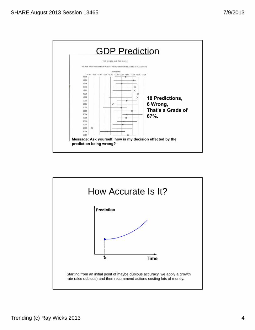
How Accurate Is It?
Time
Prediction
t0
Starting from an initial point of maybe dubious accuracy, we apply a growth rate (also dubious) and then recommend actions costing lots of money.
SHARE August 2013 Session 13465 7/9/2013
Trending (c) Ray Wicks 2013 5
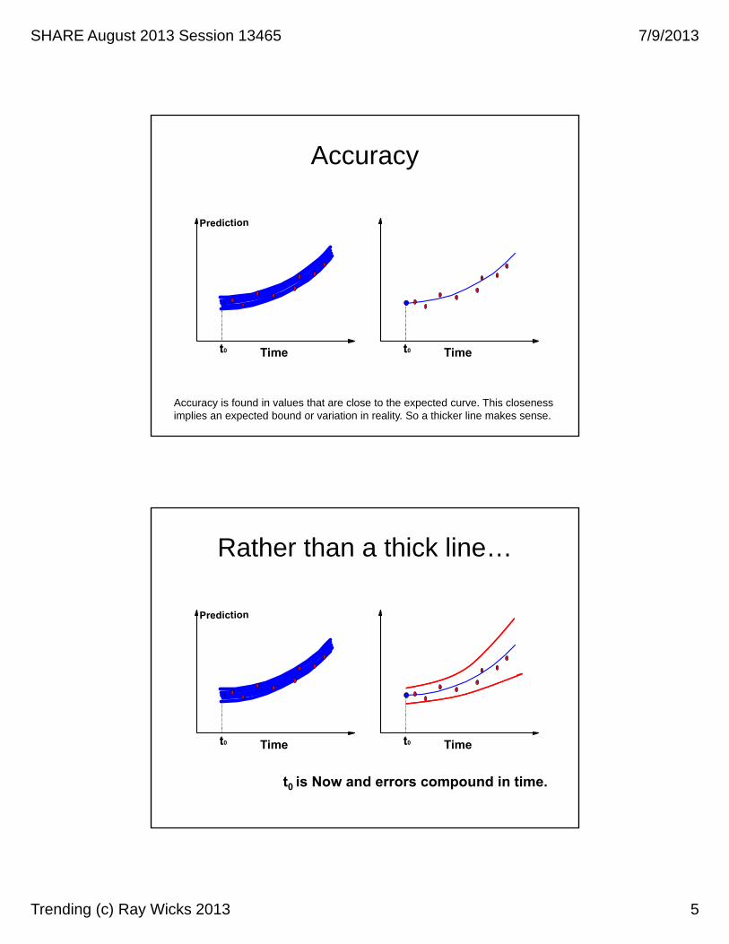
Accuracy
Timet0Time
Prediction
t0
Accuracy is found in values that are close to the expected curve. This closeness implies an expected bound or variation in reality. So a thicker line makes sense.
Rather than a thick line…
Timet0Time
Prediction
t0
t0 is Now and errors compound in time.

SHARE August 2013 Session 13465 7/9/2013
Trending (c) Ray Wicks 2013 6
How Accurate Is It?
Time
Prediction
t0 t
p
Time
Prediction
t0 t
p
At time t, is the prediction a precise point p or a fuzzy patch?

SHARE August 2013 Session 13465 7/9/2013
Trending (c) Ray Wicks 2013 7
Accuracy
Message: How far off the line is too far? And, I better track this stuff.
A Conversation
You: The answer is 42.67.
Them: I measured it and the answer is 42.663!
You: Give me a break.
Them: I just want to be exact.
You: OK the answer is around 42.67.
Them: How far around.
You: ????

SHARE August 2013 Session 13465 7/9/2013
Trending (c) Ray Wicks 2013 8
Fuzzy Expectations: X is around 42.67or X-42.67 ≈ 0or X-42.67 ≤ ∆
42.67
Around 42.67 = if you pick a number on [42.67- ∆, 42.67+ ∆] it is as good as equal 42.67.
42.67+∆42.67-∆
How to define ∆?
Fuzzy Expectations or Fuzzy Reality?
Probability of Expected Value
Expected ValueThe expected value could move within this bound if the experiment was repeated with higher probability of it being close to the center.

SHARE August 2013 Session 13465 7/9/2013
Trending (c) Ray Wicks 2013 9
Confidence Interval
[ μ – 1.96 σ/n , μ + 1.96 σ/n ]
[ μ – zα/2 σ/n , μ + zα/2 σ/n ]
Using a Standard Normal Probability table, 95% confidence (2 tail) is found by looking for a z score of 0.025.
In Excel: =Confidence(μ, σ, n)
=Confidence(0.5,1,100) = 1.96
SummaryGiven a list of numbers X={Xi} i=1 to n
StatisticsTerm Formula Excel PS ViewCount (number of items) n
=Count(X)Number of points plotted
Average X=Sum(X)/n =Average(X) Center of gravityMedian§ X[ROUND DOWN 1+N*0.5] =MEDIAN(X) Middle numberVariance V=(Xi-X)2)/n =Var(X) Spread of data
Standard Deviation s=SQRT(V) =Stnd(X) Spread of dataCoeficient of Variation (Std/Avg) CV=s/X
Spread of data around average
Minimum First in Sorted list =MIN(X) Bottom of plotMaximum Last in Sorted list =Max(X) Top of plotRange
[Minimum,Maximum]Distance between top and bottom
90th percentile§ X[ROUND DOWN 1+n*0.9] =Percentile(X,0.9) 10% from the topConfidence interval
Look in book =Confidence(0.05,s,n)Expected Variability of average (a thick line)
§= Percentile formulae assume a sorted list; Low to high.

SHARE August 2013 Session 13465 7/9/2013
Trending (c) Ray Wicks 2013 10
Correlation & Prediction
0
100
200
300
400
500
600
700
800
900
1000
0 10 20 30 40 50
Var 1
Var
2
Random with correlation = 0
The Intent of regression analysisGiven a set of paired observations {(xi,yi)} for i=1 to nThe goal is to develop a function that uses X as a predictor of Y.Y = f(X) such that yi-yi is minimal. Or Yi = Yi + e where e is the error term.
Question: Does X cause (correlate, act as a predictor) of Y?
A concern when X is Time. Given {(ti,yi)}, can time be a cause? If T is peak daily period and Y is CPU%, does time of day cause CPU% level? No it is a correlate.

SHARE August 2013 Session 13465 7/9/2013
Trending (c) Ray Wicks 2013 11
Briefly: Correlation is not Causality
Cause → Effect (sufficient cause)~Effect → ~Cause (necessary cause)
R2 or CORR(C,E) may indicate a linear relationship without there being a causal connection.
In cities of various sizes: C = number of TVs is highly correlated with E = number of murders. C = religious events is highly correlated with E = number of suicides.
Causality & CorrelationClaim: Eating Cheerios will lower your cholesterolCause → EffectCause: Eating CheeriosEffect: Lower Cholesterol
Test: Real causeIntervening Variable
Bacon & Eggs Cholesterol
Cheerios Lower Cholesterol
Bacon & Eggs Lower Cholesterol
There is a correlation between Eating Cheerios and lowerCholesterol but is there a causal relationship?
X
SHARE August 2013 Session 13465 7/9/2013
Trending (c) Ray Wicks 2013 12
Interesting Correlations1. The Japanese eat very little fatand suffer fewer heart attacks than Americans.
2. The Mexicans eat a lot of fatand suffer fewer heart attacks than Americans.
3. The Chinese drink very little red wine and suffer fewer heart attacks than Americans.
4. The Italians drink a lot of red wineand suffer fewer heart attacks than Americans.
5. The Germans drink a lot of beers and eat lots of sausages and fats and suffer fewer heart attacks than Americans.
CONCLUSION?
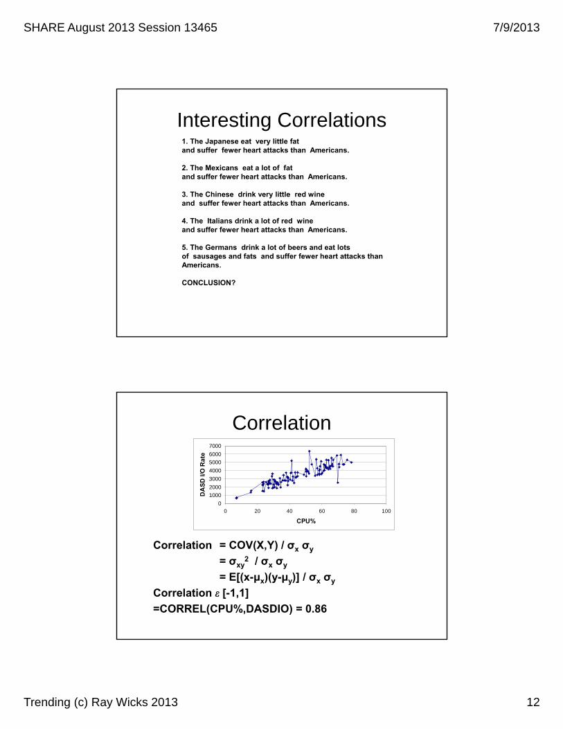
Correlation
0
1000
2000
3000
4000
5000
6000
7000
0 20 40 60 80 100
CPU%
DA
SD
I/O
Ra
te
Correlation = COV(X,Y) / σx σy
= σxy2 / σx σy
= E[(x-μx)(y-μy)] / σx σy
Correlation [-1,1]
=CORREL(CPU%,DASDIO) = 0.86

SHARE August 2013 Session 13465 7/9/2013
Trending (c) Ray Wicks 2013 13
The B.S. Model
y = 60.941x + 655.76
R2 = 0.8377
0
1000
2000
3000
4000
5000
6000
7000
0 10 20 30 40 50 60 70 80
CPU%
DA
SD
I/O
DASD
DASD
GKWE
Thinking
CPU
Memory
Our B.S. model anticipates a correlation between CPU time and DASD rate.
Linear Fit
y = 59.877x + 733.8
R2 = 0.7425
01000
20003000
40005000
60007000
0 20 40 60 80 100
CPU%
DA
SD
I/O
Rat
e

SHARE August 2013 Session 13465 7/9/2013
Trending (c) Ray Wicks 2013 14
Predictive Analysis Given {Xi,Yi} i=1,n
Find Yi=F(Xi) such that the sum of errors squared is minimized (Sum(Yi – Yi)2 )
The evaluate F(Xi) from i = n+1 to n+j (j future periods/values)
y = 0.0588x + 8.7307R2 = 0.7978
0
10
20
30
40
50
60
70
80
0 200 400 600 800 1000 1200
Block Count
CP
U%
Y=0.0588x + 8.7307
Y=0.0588*1000 + 8.7307
Y = 67.5%
Linear Regression
y = 3.0504x + 385.42
R2 = 0.7881
0
100
200
300
400
500
600
700
800
900
1000
0 50 100 150 200
Week
MIP
S U
sed

SHARE August 2013 Session 13465 7/9/2013
Trending (c) Ray Wicks 2013 15
Reality
y = 3.0504x + 385.42
R2 = 0.7881
0
200
400
600
800
1000
1200
1400
1600
1800
0 50 100 150 200
Week
MIP
S U
sed
Linear regression’s predictions assume that the future looks like the past.
Linear Fit for {Xi,Yi}
X
Y
Yi=B0 + B1Xi
Xi
Yi
Yi
e
B0
Y
(Yi - Y)2
(Yi - Y)2
On the line would be perfect. Next to that would be a line with minimum error (e). Actually minimum e2 is better.
Goodness of Fit R2 =

SHARE August 2013 Session 13465 7/9/2013
Trending (c) Ray Wicks 2013 16
Excel Help
Search Excel Help for R Squared return:
RSQ: Returns the square of the Pearson product moment correlation coefficient through data points in known_y's and known_x's. For more information, see PEARSON. The r-squared value can be interpreted as the proportion of the variance in y attributable to the variance in x.
Matrix Solution for Linear FitB = (Mt * M)-1 * Mt * Y
Solve for Y = B0 + B1*X X Y YH Sq (YH-YA) Sq (Y-YA) R2
M is 5x2 1 62.3 1.3 1.316809 0.0151761 0.0196 0.819061 =(SUM(F3:F7)/SUM(G3:G7))1 64.3 1.4 1.354367 0.007333 0.00161 70.8 1.4 1.476432 0.0013273 0.00161 71.1 1.5 1.482065 0.0017695 0.00361 75.8 1.6 1.570328 0.0169853 0.0256
Avg 1.44
MT is 2x5 1 1 1 1 1 ctl-shift-enter62.3 64.3 70.8 71.1 75.8
MT*M is 2x2 5 344.3344.3 23829.27
INV(MTM) is 2x2 39.46158 -0.57017-0.57017 0.00828
IMTM*MT is 2x5 3.940284 2.799954 -0.90612 -1.07717 -3.756947-0.05432 -0.03776 0.016063 0.018547 0.0574637
IMTMMT*Y is 2x1 0.146865 B00.018779 B1

SHARE August 2013 Session 13465 7/9/2013
Trending (c) Ray Wicks 2013 17
Excel Solution
y = 0.0188x + 0.1469
R2 = 0.8191
1.21.251.3
1.351.4
1.451.5
1.551.6
1.65
60 65 70 75 80
X
Y
Impact of Outlier
y = -0.0058x + 1.9284
R2 = 0.0174
1.21.3
1.41.51.6
1.71.81.9
22.1
60 65 70 75 80
Y
Linear (Y)

SHARE August 2013 Session 13465 7/9/2013
Trending (c) Ray Wicks 2013 18
A perfect fit is always possible
y = 58111x4 - 338194x3 + 736689x2 - 711801x + 257442
R2 = 1
50
55
60
65
70
75
80
1.2 1.25 1.3 1.35 1.4 1.45 1.5 1.55 1.6 1.65
Units of Work
CP
U%
Albeit meaningless in this case.
Goodness of Fit.
Residual
-2.5
-2
-1.5
-1
-0.5
0
0.5
1
1.5
2
2.5
1.1
Units of Work
Re
sid
ua
l
Residual = Yi – YpredictThe plot of residuals should show points randomly distributed around 0.

SHARE August 2013 Session 13465 7/9/2013
Trending (c) Ray Wicks 2013 19
EXCEL Solutiony = 47.3x + 0.275
R2 = 0.9262
50
55
60
65
70
75
80
1.2 1.3 1.4 1.5 1.6 1.7
Units of Work
CP
U%
Units of Work (X) CPU% (Y) YH=47.3x + 0.275 Residual=Yi-Yhi Resid*21.3 62.3 61.765 0.535 0.2862251.4 64.3 66.495 -2.195 4.818025
1.45 70.8 68.86 1.94 3.76361.5 71.1 71.225 -0.125 0.0156251.6 75.8 75.955 -0.155 0.024025
SSE 8.9075Syx 1.723127002Avg X 1.45sum(xi-avgx)*2T 3.182446305N 5
Solution with Bounds
y = 47.3x + 0.275
R2 = 0.9262
5055606570758085
1.2 1.3 1.4 1.5 1.6 1.7
Units of Work
CP
U%
CPU%
LB
UB
Linear (CPU%)
Linear (CPU%)

SHARE August 2013 Session 13465 7/9/2013
Trending (c) Ray Wicks 2013 20
ComputationsUnits of Work (X) CPU% (Y) YH=47.489x + 0.275Residual=Yi-Yhi Resid*2(Xi-Avgx)*2 Comp LB UB
1.3 62.3 61.765 0.535 0.286225 0.0225 0.65 57.34385 66.186151.4 64.3 66.495 -2.195 4.818025 0.0025 0.25 63.75312 69.23688
1.45 70.8 68.86 1.94 3.7636 0 0.2 66.40759 71.312411.5 71.1 71.225 -0.125 0.015625 0.0025 0.25 68.48312 73.966881.6 75.8 75.955 -0.155 0.024025 0.0225 0.65 71.53385 80.37615
1.65 78.32 1 72.83624 83.803761.7 80.685 1.45 74.08168 87.28832
1.75 83.05 2 75.29479 90.805211.8 85.415 2.65 76.48809 94.34191
SSE 8.9075Syx 1.723127002Avg X 1.45sum(xi-avgx)*2 0.05T 3.182446305N 5
Comp: =(1/ROWS(X))+(POWER(A2-Avgx,2))/$F$14
LB: =$C2-T*Sxy*SQRT($G2)
Projection with Bounds
y = 47.3x + 0.275
R2 = 0.9262
50
60
70
80
90
100
1.2 1.4 1.6 1.8 2
Units of Work
CP
U% CPU%
LB
UB
Linear (CPU%)

SHARE August 2013 Session 13465 7/9/2013
Trending (c) Ray Wicks 2013 21
Projection with Bounds
y = 47.3x + 0.275
R2 = 0.9262
50
60
70
80
90
100
1.2 1.4 1.6 1.8 2
Units of Work
CP
U% CPU%
LB
UB
Linear (CPU%)
Y=mX for CPU% vs Blocks/Sec
y = 0.0235x
R2 = -0.7761
0
10
20
30
40
50
60
70
0 1000 2000 3000
Blocks/sec
CP
U%
(b=0 in Y=mX + b)

SHARE August 2013 Session 13465 7/9/2013
Trending (c) Ray Wicks 2013 22
Filtered Data CPU%>10
y = 0.0742x
R2 = 0.9028
0
10
20
30
40
50
60
70
0 200 400 600 800 1000
Blocks/sec
CP
U%
Residuals
For each Xi, plot e = Y- Yi
Residual
-20
-15
-10
-5
0
5
10
0 100 200 300 400 500 600 700 800 900
Units of Work
Re
sid
ua
l
SHARE August 2013 Session 13465 7/9/2013
Trending (c) Ray Wicks 2013 23
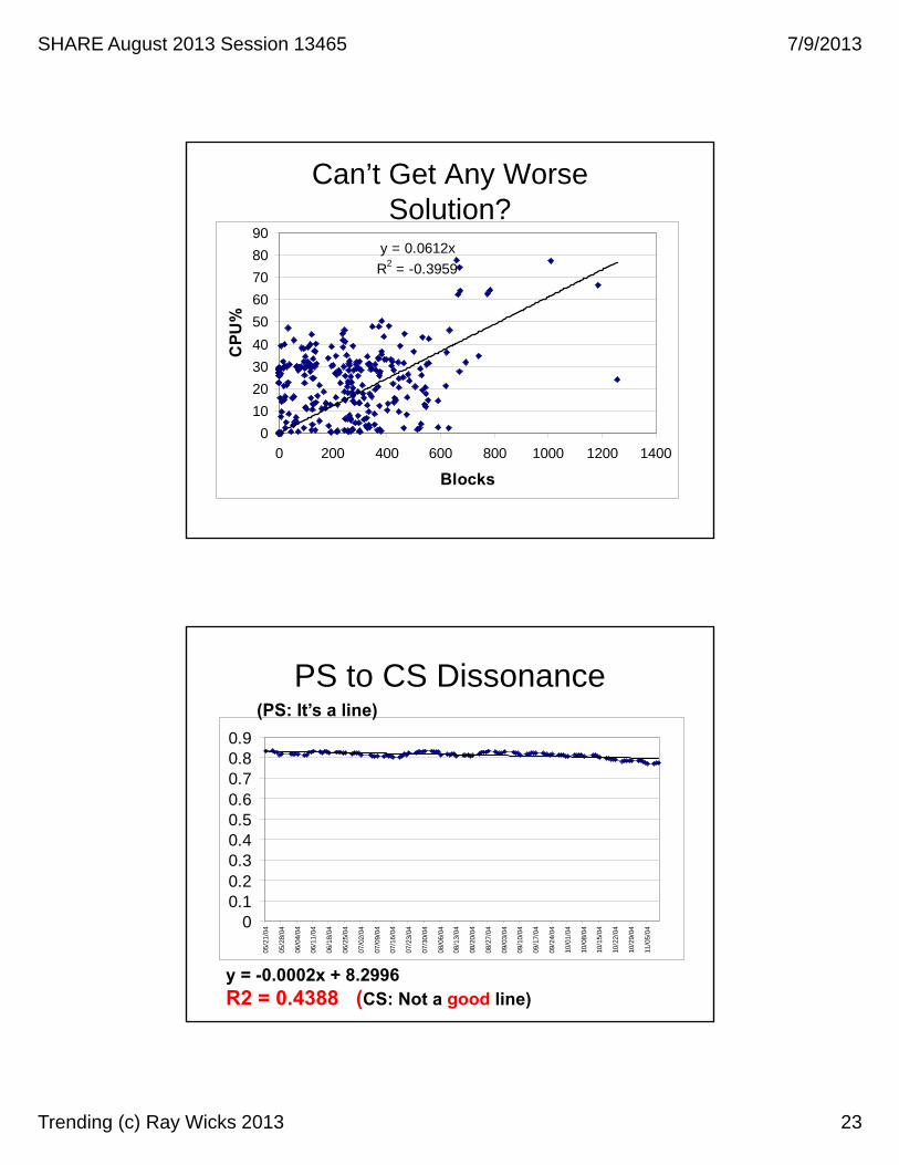
Can’t Get Any WorseSolution?
y = 0.0612x
R2 = -0.3959
0
10
20
30
40
50
60
70
80
90
0 200 400 600 800 1000 1200 1400
Blocks
CP
U%
PS to CS Dissonance
00.10.20.30.40.50.60.70.80.9
05/2
1/04
05/2
8/04
06/0
4/04
06/1
1/04
06/1
8/04
06/2
5/04
07/0
2/04
07/0
9/04
07/1
6/04
07/2
3/04
07/3
0/04
08/0
6/04
08/1
3/04
08/2
0/04
08/2
7/04
09/0
3/04
09/1
0/04
09/1
7/04
09/2
4/04
10/0
1/04
10/0
8/04
10/1
5/04
10/2
2/04
10/2
9/04
11/0
5/04
(PS: It’s a line)
y = -0.0002x + 8.2996R2 = 0.4388 (CS: Not a good line)
SHARE August 2013 Session 13465 7/9/2013
Trending (c) Ray Wicks 2013 24
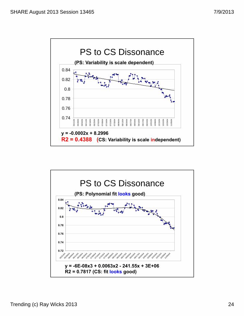
PS to CS Dissonance
0.74
0.76
0.78
0.8
0.82
0.8405
/21/
04
05/2
8/04
06/0
4/04
06/1
1/04
06/1
8/04
06/2
5/04
07/0
2/04
07/0
9/04
07/1
6/04
07/2
3/04
07/3
0/04
08/0
6/04
08/1
3/04
08/2
0/04
08/2
7/04
09/0
3/04
09/1
0/04
09/1
7/04
09/2
4/04
10/0
1/04
10/0
8/04
10/1
5/04
10/2
2/04
10/2
9/04
11/0
5/04
y = -0.0002x + 8.2996R2 = 0.4388 (CS: Variability is scale independent)
(PS: Variability is scale dependent)
PS to CS Dissonance
y = -6E-08x3 + 0.0063x2 - 241.55x + 3E+06R2 = 0.7817 (CS: fit looks good)
0.72
0.74
0.76
0.78
0.8
0.82
0.84
05/21
/04
05/28
/04
06/04
/04
06/11
/04
06/18
/04
06/25
/04
07/02
/04
07/09
/04
07/16
/04
07/23
/04
07/30
/04
08/06
/04
08/13
/04
08/20
/04
08/27
/04
09/03
/04
09/10
/04
09/17
/04
09/24
/04
10/01
/04
10/08
/04
10/15
/04
10/22
/04
10/29
/04
11/05
/04
(PS: Polynomial fit looks good)

SHARE August 2013 Session 13465 7/9/2013
Trending (c) Ray Wicks 2013 25
???
0
0.1
0.2
0.3
0.4
0.5
0.6
0.7
0.8
0.905
/21/
04
06/0
4/04
06/1
8/04
07/0
2/04
07/1
6/04
07/3
0/04
08/1
3/04
08/2
7/04
09/1
0/04
09/2
4/04
10/0
8/04
10/2
2/04
11/0
5/04
11/1
9/04
12/0
3/04
12/1
7/04
12/3
1/04
01/1
4/05
01/2
8/05
02/1
1/05
02/2
5/05
03/1
1/05
03/2
5/05
In 144 Days, the $ will be worthless.
Trending: What to DO?
Average In & Ready
0
5
10
15
20
25
30
35
40
0 100 200 300 400
90th%ile
SHARE August 2013 Session 13465 7/9/2013
Trending (c) Ray Wicks 2013 26
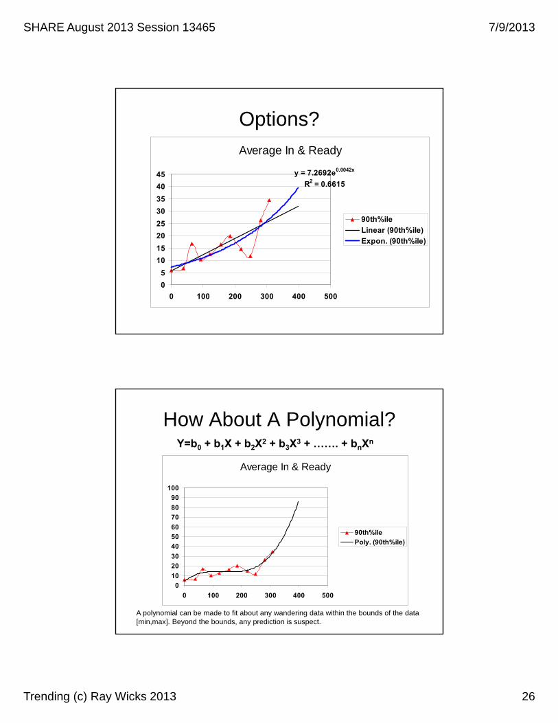
Options?
Average In & Ready
y = 7.2692e0.0042x
R2 = 0.6615
0
5
10
15
20
25
30
35
40
45
0 100 200 300 400 500
90th%ile
Linear (90th%ile)
Expon. (90th%ile)
How About A Polynomial?
Average In & Ready
0
10
20
30
40
50
60
70
80
90
100
0 100 200 300 400 500
90th%ile
Poly. (90th%ile)
A polynomial can be made to fit about any wandering data within the bounds of the data [min,max]. Beyond the bounds, any prediction is suspect.
Y=b0 + b1X + b2X2 + b3X3 + ……. + bnXn

SHARE August 2013 Session 13465 7/9/2013
Trending (c) Ray Wicks 2013 27
A time series is a sequence of observations which are ordered in time (or space). If observations are made on some phenomenon throughout time, it is most sensible to display the data in the order in which they arose, particularly since successive observations will probably be dependent. Time series are best displayed in a scatter plot. The series value X is plotted on the vertical axis and time t on the horizontal axis. Time is called the independent variable (in this case however, something over which you have little control). There are two kinds of time series data: 1. Continuous, where we have an observation at every instant of time e.g. lie detectors, electrocardiograms. We denote this using observation X at time t, X(t). 2. Discrete, where we have an observation at (usually regularly) spaced intervals. We denote this as Xt.
Time Series
See http://www.cas.lancs.ac.uk/glossary_v1.1/tsd.html#timeseries
Time Series Models (Briefly)(Box-Jenkins Analysis)

SHARE August 2013 Session 13465 7/9/2013
Trending (c) Ray Wicks 2013 28
Poor Mans Time Series
INDEX AIR Diff 11 5.92 6.7 0.83 16.8 10.14 10.3 -6.55 12.4 2.16 16.5 4.17 19.9 3.48 14.6 -5.39 11.7 -2.9
10 26.3 14.611 34.5 8.2
Input AIR
0
5
10
15
20
25
30
35
40
0 2 4 6 8 10 12
Period
AIR AIR
Difference 1
-10
-5
0
5
10
15
20
0 2 4 6 8 10 12
Period
Dif
f
Ref: TSERDAT.xls
A 1 2-3 2.5
B 0 -17 2
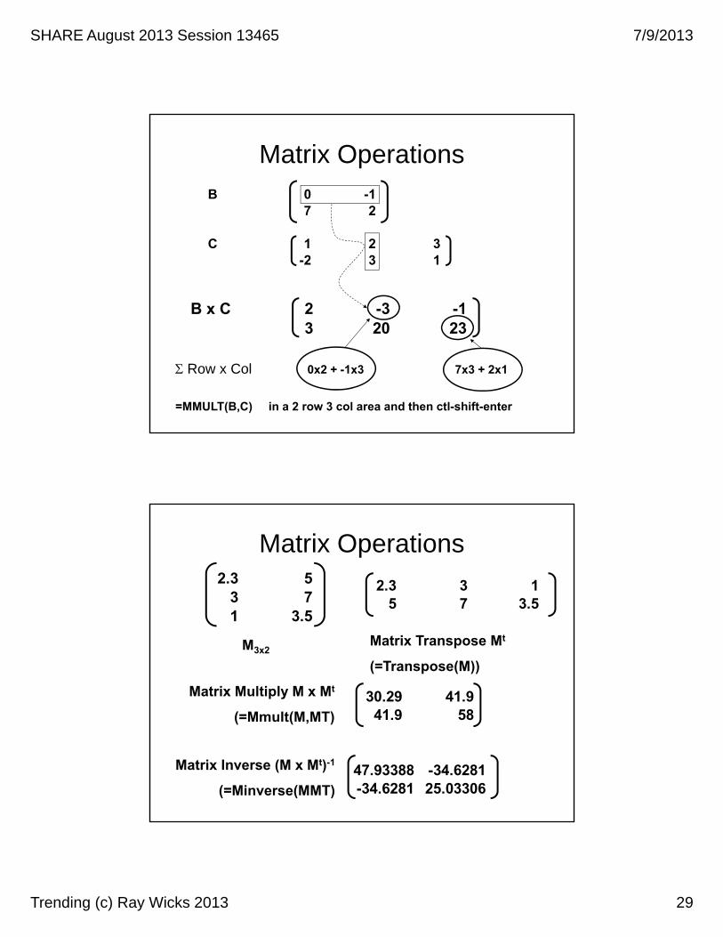
Matrix Operations
A+B 1 14 4.5
SHARE August 2013 Session 13465 7/9/2013
Trending (c) Ray Wicks 2013 29
B 0 -17 2
C 1 2 3-2 3 1
Matrix Operations
B x C 2 -3 -13 20 23
Row x Col 0x2 + -1x3 7x3 + 2x1
=MMULT(B,C) in a 2 row 3 col area and then ctl-shift-enter
Matrix Operations2.3 5
3 71 3.5
2.3 3 15 7 3.5
30.29 41.941.9 58
47.93388 -34.6281-34.6281 25.03306
M3x2Matrix Transpose Mt
(=Transpose(M))
Matrix Multiply M x Mt
(=Mmult(M,MT)
Matrix Inverse (M x Mt)-1
(=Minverse(MMT)

SHARE August 2013 Session 13465 7/9/2013
Trending (c) Ray Wicks 2013 30
Matrix Operations
30.29 41.941.9 58
47.93388 -34.6281-34.6281 25.03306
X
1 4.54747E-130 1
The Ugly Part
INDEX AIR Diff 11 5.92 6.7 0.83 16.8 10.14 10.3 -6.55 12.4 2.16 16.5 4.17 19.9 3.48 14.6 -5.39 11.7 -2.9
10 26.3 14.611 34.5 8.2
Y X0 X1 X2 X32.1 1 0.8 10.1 -6.54.1 1 10.1 -6.5 2.13.4 1 -6.5 2.1 4.1
-5.3 1 2.1 4.1 3.4-2.9 1 4.1 3.4 -5.314.6 1 3.4 -5.3 -2.98.2 1 -5.3 -2.9 14.6
Y = b0 + b1X1 + b2X2 +b3X3Or
X4 = b0 + b1X1 + b2X2 +b3X3
From the input variable AIR, form the pair wise difference sequence Diff 1 = xn – xn-1. Then build the matrix M for order 3 solution.
Y M

SHARE August 2013 Session 13465 7/9/2013
Trending (c) Ray Wicks 2013 31
With a Little MagicSolve for B
B = (Mt * M)-1 * Mt * Y* = Matrix multiplyB0= 6.493 B1= -0.951 B2= -1315 B3= -0.673
//WICKS JOB (????,????),WICKS,MSGLEVEL=1,MSGCLASS=O,NOTIFY=WICKS //SAS EXEC SAS //SYSIN DD * OPTIONS LINESIZE=80 NOCENTER;
DATA CAPTURE; INPUT Y X1-X3;CARDS;
2.1 0.8 10.1 -6.54.1 10.1 -6.5 2.13.4 -6.5 2.1 4.1-5.3 2.1 4.1 3.4-2.9 4.1 3.4 -5.314.6 3.4 -5.3 -2.98.2 -5.3 -2.9 14.6 PROC REG; MODEL Y = X1-X3 ;
SAS:
Or Excel ►
Excel Steps for Multiple Regression
X0 X1 X2 X31 0.8 10.1 -6.51 10.1 -6.5 2.11 -6.5 2.1 4.11 2.1 4.1 3.41 4.1 3.4 -5.31 3.4 -5.3 -2.91 -5.3 -2.9 14.6
Y = b0 + b1X1 + b2X2 +b3X3B = (Mt * M)-1 * Mt * Y
1 1 1 1 1 1 10.8 10.1 -6.5 2.1 4.1 3.4 -5.3
10.1 -6.5 2.1 4.1 3.4 -5.3 -2.9-6.5 2.1 4.1 3.4 -5.3 -2.9 14.6
M =[7 x 4]
Mt = Transpose(M) =[4 x 7]

SHARE August 2013 Session 13465 7/9/2013
Trending (c) Ray Wicks 2013 32
More Steps
5 9.5-51.32 -112.47213.54 -101.74
-101.74 324.69
Y = b0 + b1X1 + b2X2 +b3X3B = (Mt * M)-1 * Mt * Y
0.228013 -0.02868 -0.02368 -0.02402-0.02868 0.011571 0.006773 0.006969-0.02368 0.006773 0.009772 0.006101-0.02402 0.006969 0.006101 0.008108
MTM= Mt * M = MMULT(MT,M) = [4 x 7]*[7 x 4] = [4 x 4]
invMTM = Inverse(MTM) =[4 x 4]
More Steps
6.492618-0.95067-1.31524-0.67382
Y = b0 + b1X1 + b2X2 +b3X3B = (Mt * M)-1 * Mt * Y
invMTMMT = MMULT( invMTM,MT) =[4 x 4]*[4 x 7] = [4 x7]
SOLB = MULT(invMTMMT.Y) =[4 x 7]*[7 x 1] = [4 x 1]
0.122092 0.041831 0.266191 -0.01096 0.157264 0.325667 0.0979160.003684 0.0588 -0.06109 0.047085 0.004853 -0.04544 -0.007890.040781 -0.00598 -0.02217 0.051352 0.004981 -0.07013 0.00116-0.00954 0.023739 -0.02327 0.043193 -0.01768 -0.05618 0.039731

SHARE August 2013 Session 13465 7/9/2013
Trending (c) Ray Wicks 2013 33
The Prediction
INDEX AIR Diff 1 Pred Diff 1 Pred AIR1 5.92 6.7 0.83 16.8 10.14 10.3 -6.55 12.4 2.1 -3.17 7.136 16.5 4.1 4.02 16.427 19.9 3.4 7.15 23.658 14.6 -5.3 -3.19 16.719 11.7 -2.9 1.69 16.29
10 26.3 14.6 12.19 23.8911 34.5 8.2 5.51 31.8112 -15.48 19.0213 -7.74 11.2814 24.27 35.5515 15.04 50.5916 -28.20 22.39
Xn = 6.493 - 0.951Xn-1 -1315Xn-2 -0.673Xn-3
=+
Diff 1 Plot
Difference 1
-40
-30
-20
-10
0
10
20
30
0 5 10 15 20
Period
Dif
f Diff 1
Pred Diff 1

SHARE August 2013 Session 13465 7/9/2013
Trending (c) Ray Wicks 2013 34
Prediction for AIR
AIR
0
10
20
30
40
50
60
0 5 10 15 20
Period
AIR
AIR
Pred AIR
Xn = 6.493 - 0.951Xn-1 -1315Xn-2 -0.673Xn-3
R2 = 0.89
Bibliography
Statistical Concepts and Methods, Bhattacharyya & Johnson, Wiley, 1977. This has both a discussion of meaning and the formulae.
Applied Statistics for Engineers and Scientists, Levine, Ramsey & Smidt, Prentice Hall, 2001. This has a good approach to statistics and Excel implementations. CD comes with the book.
The Art of Computer Systems Performance Analysis, by Raj Jain, Wiley. I like this one. For performance analysis and capacity planning, it is thorough and complete. A very good reference. It may be hard to find.
Applied Regression Analysis, by Draper & Smith. This is the classic in regression analysis. It can get a little deep. However, if you like a full treatment with derivations of the formulae, this is it.
The Signal and the Noise, by Nate Silver. An interesting book on real life prediction.