Tracking a maneuvering object in a noisy environment using IMMPDAF By: Igor Tolchinsky Alexander Levin Supervisor: Daniel Sigalov Spring 2006

Tracking a Tracking a maneuvering object in maneuvering object in a noisy environment a noisy environment

using IMMPDAFusing IMMPDAF By:By:

Igor TolchinskyIgor TolchinskyAlexander LevinAlexander Levin

Supervisor:Supervisor:Daniel SigalovDaniel Sigalov

Spring 2006Spring 2006

Project goalsProject goals Learn about ATC problems and the Learn about ATC problems and the

algorithms involved.algorithms involved. Implement the simulation track and the Implement the simulation track and the

tracking algorithms IMM and PDAF in tracking algorithms IMM and PDAF in MATLAB.MATLAB.

Test algorithms performance.Test algorithms performance.

Problem DefinitionProblem Definition Estimate target state (position, Estimate target state (position,

velocity and acceleration) in 2-velocity and acceleration) in 2-dimensional Cartesian coordinates.dimensional Cartesian coordinates.

The estimation overcomes the next The estimation overcomes the next problems:problems:

-Discrete sampling.-Discrete sampling. -Noisy sampling, noisy environment. -Noisy sampling, noisy environment. -Detection probability lower then 1.-Detection probability lower then 1.

Solution approachSolution approach KF - Kalman Filter: a linear filter that KF - Kalman Filter: a linear filter that

estimates the state vector.estimates the state vector. IMM - Interacting Multiple Model: uses a KF IMM - Interacting Multiple Model: uses a KF

for each one of the models.for each one of the models. PDAF - Probabilistic Data Association Filter: PDAF - Probabilistic Data Association Filter:

statistical approach that deals with false statistical approach that deals with false alarms. alarms.

IMMPDAF - Combining both algorithms in IMMPDAF - Combining both algorithms in order to estimate the state vector of order to estimate the state vector of maneuvering object in noisy environment.maneuvering object in noisy environment.

Kalman FilterKalman Filter KF estimates the state of a discrete KF estimates the state of a discrete

time controlled process that is time controlled process that is governed by the linear difference governed by the linear difference equation:equation:

KF uses recursive solution:KF uses recursive solution:

1 1 1n

k k k k

mk k k

x Ax Bu w x R state vector

z Hx v z R measurement state

1 1

1

ˆ ˆk k k

Tk k

x Ax BuTime update equations

P AP A Q

1( )

ˆ ˆ ˆ( )

( )

T Tk k k

k k k k k

k k k

K P H HP H R

x x K z Hx Measurement update equations

P I K H P

IMM - Interacting Multiple IMM - Interacting Multiple ModelModel

Defining the number and the kind of Defining the number and the kind of models for the algorithm (each models for the algorithm (each model is Kalman-Filter based).model is Kalman-Filter based).

Calculating the probability for each Calculating the probability for each model, by using a-priori probabilities model, by using a-priori probabilities and transition matrix.and transition matrix.

Combining the estimations of each Combining the estimations of each model in order to estimate the state model in order to estimate the state vector.vector.

IMM treats maneuvering problems by:IMM treats maneuvering problems by:

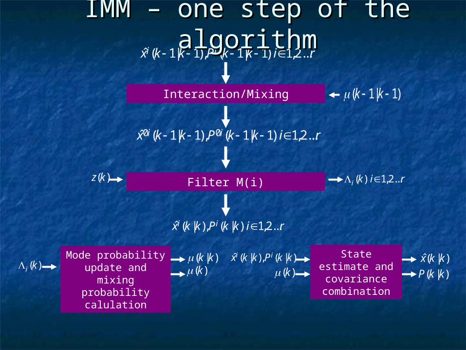
( 1| 1), ( 1| 1) 1,2...ˆi ix k k P k k i r

Interaction/Mixing ( 1| 1)k k

0 0( 1| 1), ( 1| 1) 1,2...ˆ i ix k k P k k i r

Filter M(i)( )z k ( ) 1,2...i k i r

ˆ ( | ), ( | ) 1,2...i ix k k P k k i r

Mode probability update and mixing

probability calulation

State estimate and covariance

combination( )i k

( | )k k( )k ( )k

ˆ ( | ), ( | )i ix k k P k k ˆ( | )x k k

( | )P k k

IMM – one step of the IMM – one step of the algorithmalgorithm

PDAF – Probabilistic Data PDAF – Probabilistic Data Association FilterAssociation Filter

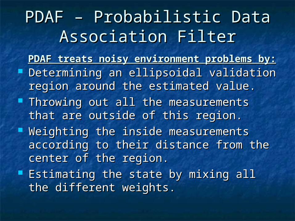
Determining an ellipsoidal validation Determining an ellipsoidal validation region around the estimated value.region around the estimated value.

Throwing out all the measurements that Throwing out all the measurements that are outside of this region.are outside of this region.

Weighting the inside measurements Weighting the inside measurements according to their distance from the center according to their distance from the center of the region.of the region.

Estimating the state by mixing all the Estimating the state by mixing all the different weights.different weights.

PDAF treats noisy environment problems by:PDAF treats noisy environment problems by:

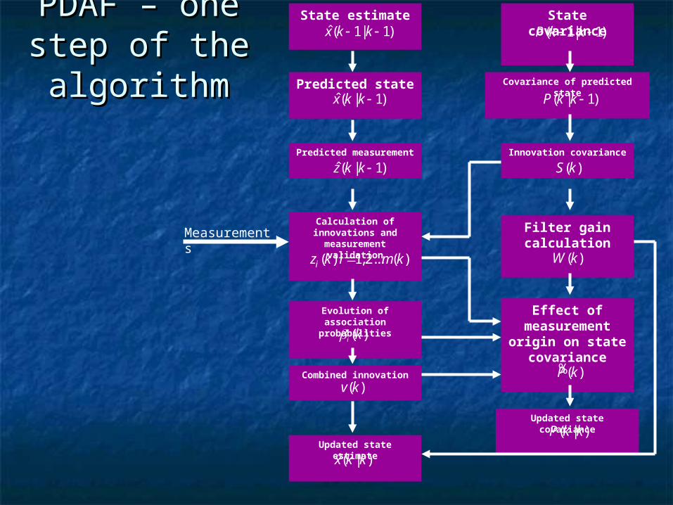
State estimateˆ( 1| 1)x k k

State covariance( 1| 1)P k k

Predicted stateˆ( | 1)x k k

Covariance of predicted state( | 1)P k k

Predicted measurementˆ( | 1)z k k

Innovation covariance

( )S k

Calculation of innovations and measurement

validation( ) 1,2... ( )iz k i m k

Filter gain calculation

( )W k

Effect of measurement origin on state

covariance( )P k%

Evolution of association

probabilities( )i k

Measurements

Combined innovation

( )v k

Updated state covariance( | )P k k

Updated state estimateˆ( | )x k k

PDAF – one step PDAF – one step of the algorithmof the algorithm

IMMPDAFIMMPDAF For each model the IMM uses a KF For each model the IMM uses a KF

and upon it’s estimation builds the and upon it’s estimation builds the validation region for the PDAF.validation region for the PDAF.

IMMPDAF treats the false alarms for IMMPDAF treats the false alarms for each model separately, and later on each model separately, and later on combines them in order to get the combines them in order to get the final state estimation.final state estimation.

Maneuvering IndexManeuvering Index The definition of the maneuvering index is The definition of the maneuvering index is

T is the sampling period and are T is the sampling period and are sampling noise and process noise sampling noise and process noise respectfully.respectfully.

As we’ll see in the next slides the value of As we’ll see in the next slides the value of the maneuvering index has a great influence the maneuvering index has a great influence on algorithm’s performance. Moreover, on algorithm’s performance. Moreover, smart definition of the model covariance can smart definition of the model covariance can optimize drastically the performance.optimize drastically the performance.

2v

w

T

,v w

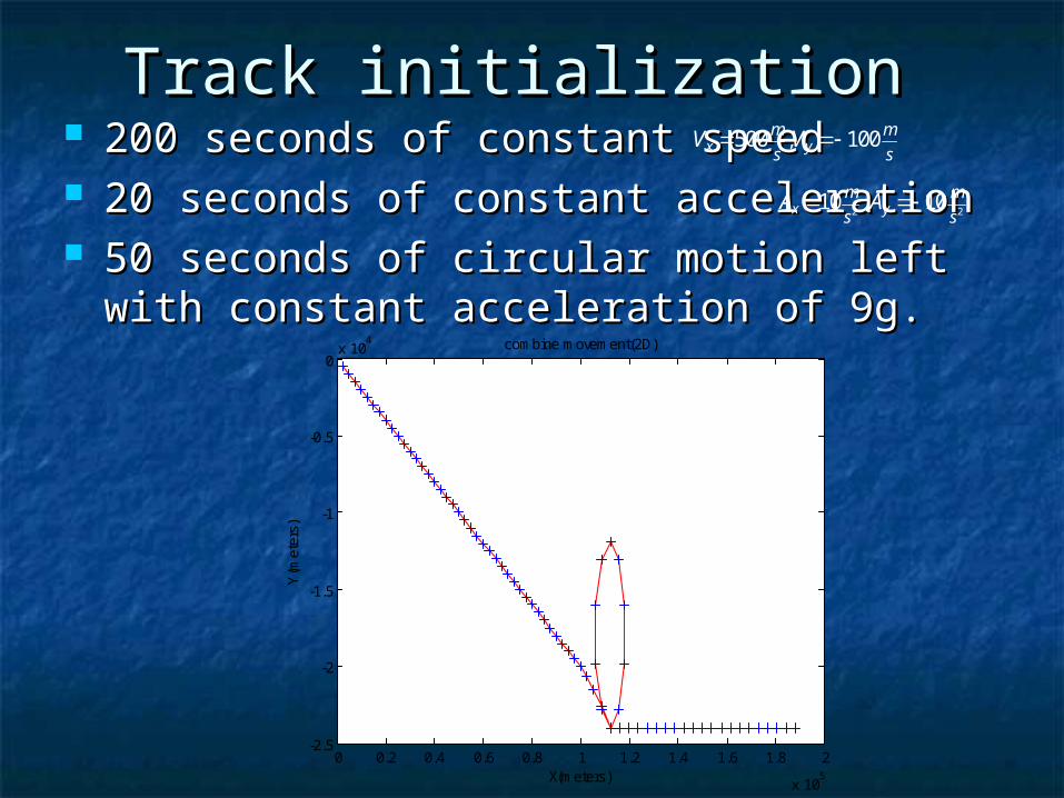
Track initialization Track initialization 200 seconds of constant speed200 seconds of constant speed 20 seconds of constant acceleration20 seconds of constant acceleration 50 seconds of circular motion left with 50 seconds of circular motion left with

constant acceleration of 9g. constant acceleration of 9g.

,500 100x ym m

s sV V

2 2,10 10x y

m m

s sA A

0 0.2 0.4 0.6 0.8 1 1.2 1.4 1.6 1.8 2

x 105

-2.5

-2

-1.5

-1

-0.5

0x 10

4

X(meters)

Y(m

eter

s)

combine movement(2D)

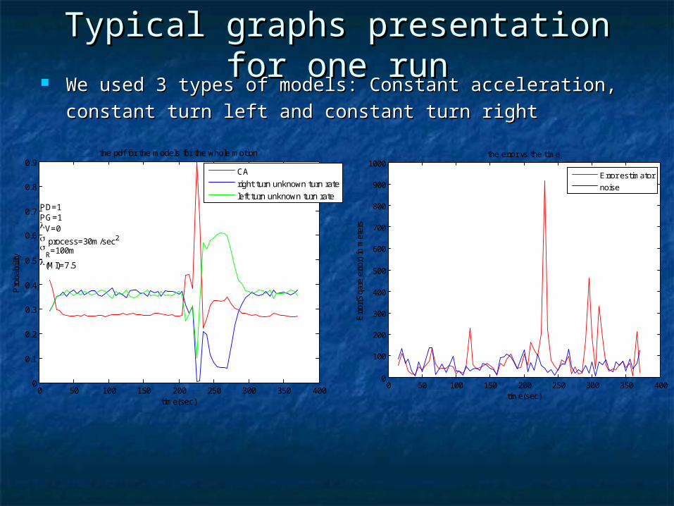
Typical graphs presentation for Typical graphs presentation for one runone run

We used 3 types of models: Constant acceleration, constant We used 3 types of models: Constant acceleration, constant

turn left and constant turn rightturn left and constant turn right

0 50 100 150 200 250 300 350 4000

0.1

0.2

0.3

0.4

0.5

0.6

0.7

0.8

0.9

time(sec)

Pro

babi

lity

the pdf for the models for the whole motion

PD=1PG=1V=0 process=30m/sec2

R=100m

(MI)=7.5

CA

right turn unknown turn rate

left turn unknown turn rate

0 50 100 150 200 250 300 350 4000

100

200

300

400

500

600

700

800

900

1000

time(sec)

Err

or(S

qare

err

or)

in m

eter

s

the error vs the time

Error estimator

noise

Typical graph presentation for Typical graph presentation for a 50 runs Monte-Carloa 50 runs Monte-Carlo

0 50 100 150 200 250 300 350 4000

100

200

300

400

500

600

700

time(sec)

RM

S-E

rror(

Sqare

err

or)

in m

ete

rs

Monte-Carlo 50runs percentage of successful runs=100%

PD=1PG=1V=50Max Error=673.3233mManeuvering RMS=182.5281mNon-Maneuvering RMS=252.5624m process=10m/sec2

R=100m

(MI)=2.5

Error estimator

average Error is 196.1459[m]

KF vs IMM comparing to Bar-KF vs IMM comparing to Bar-Shalom and Kirubarajan articleShalom and Kirubarajan article

Goals:Goals: Comparing the performances of a single KF for Comparing the performances of a single KF for

constant velocity vs 2 models IMM. Both models constant velocity vs 2 models IMM. Both models are modeling constant velocity. are modeling constant velocity. The maneuvering index of the first The maneuvering index of the first model is constant and the maneuvering index of model is constant and the maneuvering index of the second one is changing accordingly to the the second one is changing accordingly to the maneuver.maneuver.

Reconstructing the results of the article and Reconstructing the results of the article and extend the results for noisy environment (FA). extend the results for noisy environment (FA).

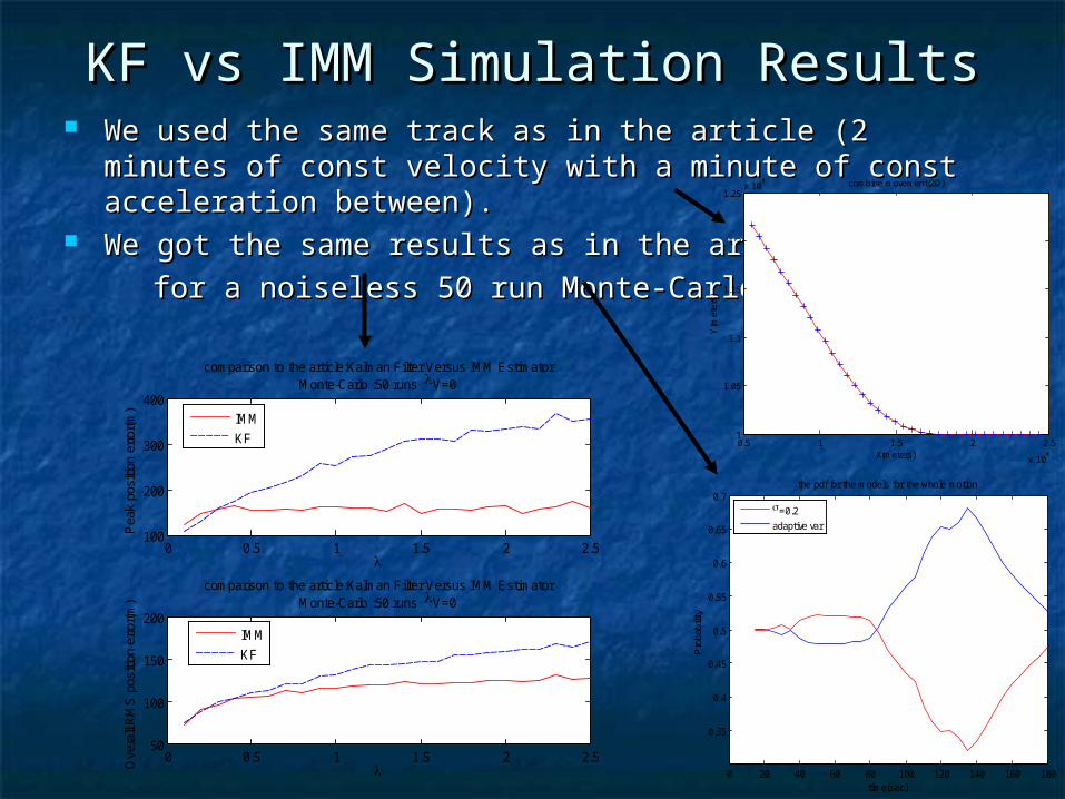
KF vs IMM Simulation ResultsKF vs IMM Simulation Results We used the same track as in the article (2 minutes of We used the same track as in the article (2 minutes of

const velocity with a minute of const acceleration between).const velocity with a minute of const acceleration between). We got the same results as in the articleWe got the same results as in the article

for a noiseless 50 run Monte-Carlo.for a noiseless 50 run Monte-Carlo.

0.5 1 1.5 2 2.5

x 104

1

1.05

1.1

1.15

1.2

1.25x 10

4

X(meters)

Y(m

eter

s)

combine movement(2D)

0 0.5 1 1.5 2 2.5100

200

300

400

Pea

k po

sitio

n er

ror(

m)

comparison to the article:Kalman Filter Versus IMM EstimatorMonte-Carlo :50 runs V=0

IMM

KF

0 0.5 1 1.5 2 2.550

100

150

200

Ove

rall

RM

S p

ositi

on e

rror

(m)


IMM

KF

0 20 40 60 80 100 120 140 160 180

0.35

0.4

0.45

0.5

0.55

0.6

0.65

0.7

time(sec)

Pro

babi

lity

the pdf for the models for the whole motion

=0.2

adaptive var

ConclusionsConclusions As expected, the performance of the As expected, the performance of the

IMM increases with the increase of IMM increases with the increase of the maneuvering index.the maneuvering index.

The intersection point is about The intersection point is about as in the article. as in the article.

0.5

Article extension – noisy Article extension – noisy environmentenvironment The number of false alarms is an independent The number of false alarms is an independent

poisson process with a known .poisson process with a known . The number of errors in this example, was 10 per The number of errors in this example, was 10 per

10 square kilometers.10 square kilometers.

0 0.5 1 1.5 2 2.5150

200

250

300

Pea

k po

sitio

n er

ror(

m)


IMM

KF

0 0.5 1 1.5 2 2.5100

120

140

160

180

Ove

rall

RM

S p

ositi

on e

rror

(m)


IMM

KF

0 0.5 1 1.5 2 2.50

20

40

60

80

Pea

k sp

eed

erro

r(m

/s)


IMM

KF

0 0.5 1 1.5 2 2.50

10

20

30

Ove

rall

RM

S s

peed

err

or(m

/s)


IMM

KF

ConclusionsConclusions In a noisy environment the difference between the In a noisy environment the difference between the

performances lowers due to the fact that the increase of performances lowers due to the fact that the increase of the maneuvering index causes wrong estimation towards the maneuvering index causes wrong estimation towards false alarms. That’s why the intersection point shifted false alarms. That’s why the intersection point shifted rightwards, .rightwards, .

The percentage of lost tracks of the IMM is always lower The percentage of lost tracks of the IMM is always lower then the one of KF, because of the maneuvering part of the then the one of KF, because of the maneuvering part of the track:track:

0.4 0.6 0.8 1 1.2 1.4 1.6 1.8 2 2.2 2.470

75

80

85

90

95

100

105

110

Per

cent

age

of s

uces

sful

run

s

percentage of successful tracking comparison to the article:Kalman Filter Versus IMM EstimatorMonte-Carlo :50 runs V=20

IMM

KF

0.8

Maneuvering index influence in Maneuvering index influence in noiseless environment noiseless environment

We used our values and got an index of about 20 in the We used our values and got an index of about 20 in the most maneuvering part (turning with constant acceleration most maneuvering part (turning with constant acceleration of 9g) of 9g)

We kept constant of 0.5 for the turning model and We kept constant of 0.5 for the turning model and changed it only for the acceleration model.changed it only for the acceleration model.

0 5 10 15 20 25200

300

400

500

Pea

k po

sitio

n er

ror(

m)

Peak Error vs lamda Monte-Carlo :5 runs best is=25PD=1 PG=1 V=0

R=100m

0 5 10 15 20 25100

150

200

250

300

Pea

k sp

eed

erro

r(m

/s)

0 5 10 15 20 2555

60

65

70

75

Ove

rall

RM

S p

ositi

on e

rror

(m)

checking for the best variance Monte-Carlo :5 runs best is=21PD=1 PG=1 V=0

R=100m

0 5 10 15 20 2522

24

26

28

30

32

Ove

rall

RM

S s

peed

err

or(m

/s)

v

500 , 100wT s m

ConclusionsConclusions At least one of the models should be with a At least one of the models should be with a

low maneuvering index and one with a high low maneuvering index and one with a high one.one.

The increase of the maneuvering index The increase of the maneuvering index improves the performance of the algorithm improves the performance of the algorithm both in maximum errors and average errors.both in maximum errors and average errors.

The algorithm performs optimally when the The algorithm performs optimally when the maneuvering index reaches it’s maximum maneuvering index reaches it’s maximum value. Furthermore increase doesn’t improve value. Furthermore increase doesn’t improve it’s performance. it’s performance.

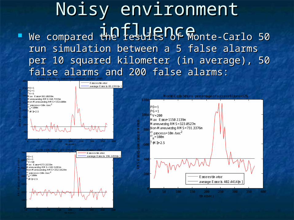
Noisy environment influenceNoisy environment influence We compared the results of Monte-Carlo 50 run We compared the results of Monte-Carlo 50 run

simulation between a 5 false alarms per 10 simulation between a 5 false alarms per 10 squared kilometer (in average), 50 false alarms squared kilometer (in average), 50 false alarms and 200 false alarms:and 200 false alarms:

0 50 100 150 200 250 300 350 4000

50

100

150

200

250

300

350

400

time(sec)

RM

S-E

rror(

Sqare

err

or)

in m

ete

rs



R=100m

(MI)=2.5

Error estimator


0 50 100 150 200 250 300 350 4000

100

200

300

400

500

600

700

time(sec)

RM

S-E

rror(

Sqare

err

or)

in m

ete

rs



R=100m

(MI)=2.5

Error estimator


0 50 100 150 200 250 300 350 4000

200

400

600

800

1000

1200

time(sec)

RM

S-E

rror

(Sqa

re e

rror

) in

met

ers



R=100m

(MI)=2.5

Error estimator


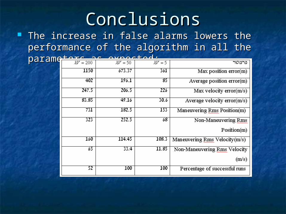
ConclusionsConclusions The increase in false alarms lowers the The increase in false alarms lowers the

performance of the algorithm in all the performance of the algorithm in all the parameters as expected:parameters as expected:

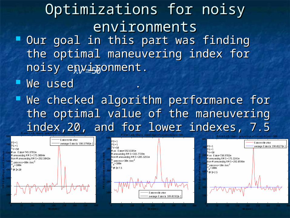
Optimizations for noisy Optimizations for noisy environmentsenvironments

Our goal in this part was finding the Our goal in this part was finding the optimal maneuvering index for noisy optimal maneuvering index for noisy environment.environment.

We used .We used . We checked algorithm performance for the We checked algorithm performance for the

optimal value of the maneuvering optimal value of the maneuvering index,20, and for lower indexes, 7.5 and index,20, and for lower indexes, 7.5 and 2.5 .2.5 .

50v

0 50 100 150 200 250 300 350 4000

100

200

300

400

500

600

700

800

time(sec)

RM

S-E

rror

(Sqa

re e

rror

) in

met

ers



R

=100m

(MI)=20

Error estimator


0 50 100 150 200 250 300 350 4000

100

200

300

400

500

600

time(sec)

RM

S-E

rror

(Sqa

re e

rror

) in

met

ers



R=100m

(MI)=7.5

Error estimator


0 50 100 150 200 250 300 350 4000

100

200

300

400

500

600

700

800

time(sec)

RM

S-E

rror

(Sqa

re e

rror

) in

met

ers



R=100m

(MI)=2.5

Error estimator


ConclusionsConclusions The optimal value of the The optimal value of the

maneuvering index in noisy maneuvering index in noisy environment is much lower then in environment is much lower then in noiseless one, due to the fact that noiseless one, due to the fact that high index causes estimation high index causes estimation towards false alarms.towards false alarms.

The last conclusions leads us to The last conclusions leads us to choose the maneuvering index of the choose the maneuvering index of the different models not only according different models not only according to the equation but also in response to the equation but also in response to the pdf of the false alarms.to the pdf of the false alarms.

Pd<1 influencePd<1 influence We changed Pd to 0.9.We changed Pd to 0.9. We worked with a noisy environment (50 We worked with a noisy environment (50

errors for 10 squared kilometers).errors for 10 squared kilometers). We choose our maneuvering index as the We choose our maneuvering index as the

optimal for this noise rate.optimal for this noise rate.

0 50 100 150 200 250 300 350 4000

200

400

600

800

1000

1200

time(sec)

RM

S-E

rror

(Sqa

re e

rror

) in

met

ers


PD=0.9PG=1V=50Max Error=1165.44mManeuvering RMS=640.2421mNon-Maneuvering RMS=530.2117m process=30m/sec2

R=100m

(MI)=7.5

Error estimator


0 50 100 150 200 250 300 350 4000

100

200

300

400

500

600

time(sec)

RM

S-E

rror

(Sqa

re e

rror

) in

met

ers



R=100m

(MI)=7.5

Error estimator


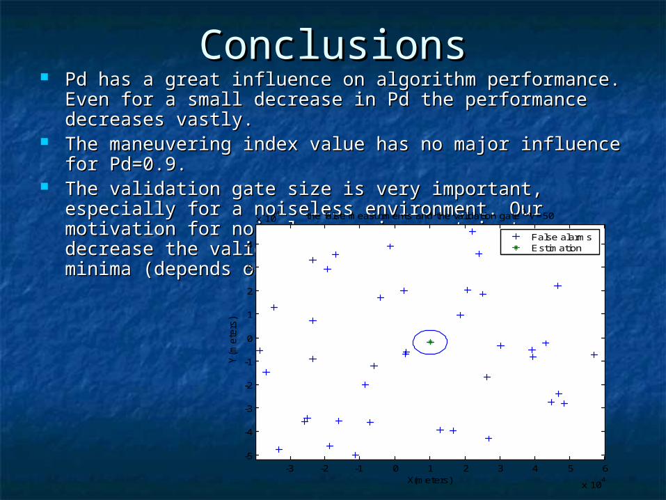
ConclusionsConclusions Pd has a great influence on algorithm performance. Even Pd has a great influence on algorithm performance. Even

for a small decrease in Pd the performance decreases for a small decrease in Pd the performance decreases vastly.vastly.

The maneuvering index value has no major influence for The maneuvering index value has no major influence for Pd=0.9.Pd=0.9.

The validation gate size is very important, especially for a The validation gate size is very important, especially for a noiseless environment. Our motivation for noiseless noiseless environment. Our motivation for noiseless environment is to decrease the validation gate for the environment is to decrease the validation gate for the potential minima (depends on object’s velocities).potential minima (depends on object’s velocities).

-3 -2 -1 0 1 2 3 4 5 6

x 104

-5

-4

-3

-2

-1

0

1

2

3

4

x 104

X(meters)

Y(m

ete

rs)

the false measurments and the validation gate V=50

False alarmsEstimation

SummarySummary We implemented the IMMPDAF in We implemented the IMMPDAF in

Matlab.Matlab. We compared our algorithm to a We compared our algorithm to a

given article and got the same given article and got the same results. Later on we extended the results. Later on we extended the conclusions for noisy environment.conclusions for noisy environment.

We analyzed algorithm’s We analyzed algorithm’s performance for different performance for different parameters.parameters.

Further workFurther work In the next part of the project we In the next part of the project we

intend to implement in Matlab an intend to implement in Matlab an algorithm which uses MCMC method algorithm which uses MCMC method in order to track unknown and in order to track unknown and uninitialized number of objects in uninitialized number of objects in noisy environment, and compare it’s noisy environment, and compare it’s performance to other recently performance to other recently proposed heuristical algorithm.proposed heuristical algorithm.

Documents

Tracking a maneuvering object in a noisy environment using IMMPDAF By: Igor Tolchinsky Alexander Levin Supervisor: Daniel Sigalov Spring 2006