Track, Check, Repeat: An EM Approach to Unsupervised Tracking

Adam W. Harley Yiming Zuo* Jing Wen* Ayush Mangal

Shubhankar Potdar Ritwick Chaudhry Katerina Fragkiadaki

Carnegie Mellon University

{aharley, yzuo, jingwen2, smpotdar, rchaudhr, katef}@cs.cmu.edu, amangal@cs.iitr.ac.in

Abstract

We propose an unsupervised method for detecting and

tracking moving objects in 3D, in unlabelled RGB-D videos.

The method begins with classic handcrafted techniques for

segmenting objects using motion cues: we estimate opti-

cal flow and camera motion, and conservatively segment

regions that appear to be moving independently of the back-

ground. Treating these initial segments as pseudo-labels,

we learn an ensemble of appearance-based 2D and 3D

detectors, under heavy data augmentation. We use this

ensemble to detect new instances of the “moving” type,

even if they are not moving, and add these as new pseudo-

labels. Our method is an expectation-maximization algo-

rithm, where in the expectation step we fire all modules and

look for agreement among them, and in the maximization

step we re-train the modules to improve this agreement. The

constraint of ensemble agreement helps combat contami-

nation of the generated pseudo-labels (during the E step),

and data augmentation helps the modules generalize to yet-

unlabelled data (during the M step). We compare against

existing unsupervised object discovery and tracking meth-

ods, using challenging videos from CATER and KITTI, and

show strong improvements over the state-of-the-art.

1. Introduction

Humans can detect moving objects and delineate their

approximate extent [54, 15], without ever having been sup-

plied boxes or segmentation masks as supervision. Where

does this remarkable ability come from? Psychology litera-

ture points to a variety of perceptual grouping cues, which

make some regions look more object-like than others [25].

These types of objectness cues have long been known in

computer vision literature [1], yet this domain knowledge

has not yet led to powerful self-supervised object detectors.

Work on integrating perceptual grouping cues into com-

puter vision models stretches back decades [51], and still

likely serves as inspiration for many of the design decisions

*Equal contribution.

in modern computer vision architectures related to atten-

tion, segmentation, and tracking. Much of the current work

on recognition and tracking is fully-supervised, and relies

on vast pools of human-provided annotations. On the un-

supervised side, a variety of deep learning-based methods

have been proposed, which hinge on reconstruction objec-

tives and part-centric, object-centric, or scene-centric bot-

tlenecks in the architecture [38, 9]. These methods are

rapidly advancing, but so far only on toy worlds, made up

of simple 2D or 3D shapes against simple backgrounds – a

far cry from the complexity tackled in older works, based

on perceptual grouping (e.g., [21]).

Classic methods of object discovery, such as center-

surround saliency in color or flow [2], are known to be brit-

tle, but they need not be discarded entirely. In this paper,

we propose to mine and exploit the admittedly rare suc-

cess scenarios of these models, to bootstrap the learning of

something more general. We hypothesize that if the suc-

cessful vs. unsuccessful runs of the classic algorithms can

be readily identified with automatic techniques, then we can

self-supervise a learning-based module to mimic and out-

perform the traditional methods. This is a kind of knowl-

edge distillation [30], from traditional models to deep ones.

We propose an optimization algorithm for learning de-

tectors of moving objects, based on expectation maximiza-

tion [45]. We begin with a motion-based handcrafted de-

tector, tuned to be very conservative (low recall, high pre-

cision). We then convert each object proposal into thou-

sands of training examples for learning-based 2D and 3D

detectors, by randomizing properties like color, scale, and

orientation. This forces the learned models to general-

ize, and allows recall to expand. We then use the ensem-

ble of models to obtain new high-confidence estimates (E

step), repeat the optimization (M step), and iterate. Our

method outperforms not only the traditional methods, which

only work under specific conditions, but also the current

learning-based methods, which only work in toy environ-

ments. We demonstrate success in a popular synthetic envi-

ronment where recent deep models have already been de-

ployed (CLEVR/CATER [34, 24]), and also on the real-

16581

world urban scenes benchmark (KITTI [23]), where the ex-

isting learned models fall flat.

Our main contribution is not in any particular compo-

nent, but rather in their combination. We demonstrate

that by exploiting the successful outcomes of traditional

methods for moving object segmentation, we can train a

learning-based method to detect and track objects in a target

domain, without requiring any annotations.

2. Related Work

Object discovery Many recent works have proposed deep

neural networks for object discovery from RGB videos.

These models typically have an object-centric bottleneck,

and are tasked with a reconstruction objective. MONet [9],

Slot attention [42], IODINE [26] , SCALOR [33], AIR [19],

and AlignNet [16] fall under this category. These methods

have been successful in a variety of simple domains, but

have not yet been tested on real-world videos. In this paper

we evaluate whether these models are able to perform well

under the complexities of real-world imagery.

Ensemble methods Using ensembles is a well-known

way to improve overall performance of an algorithm. As-

suming that each member of the ensemble is prone to dif-

ferent types of errors, the combination of them is likely to

make fewer errors than any individual component [17]. En-

sembling is also the key idea behind knowledge distillation,

where knowledge gets transferred from cumbersome mod-

els to simpler ones [30, 49]. A typical modern setup is to

make up the ensemble out of multiple copies of a neural

network, which are trained from different random initial-

izations or using different partitions of the data [3]. In our

case, the ensemble is more diverse: it is made up of com-

ponents which solve different tasks, but which can still be

checked against one another for consistency. For example,

we learn a 2D pixel labeller which operates on RGB im-

ages, and a 3D object detector which operates on voxelized

pointclouds; when the 3D detections are projected into the

image, we expect them to land on “object” pixels.

Never ending learning We take inspiration from the

methods described in “never ending learning” literature

[10, 12], where the goal is to learn an ever-increasing set

of concepts over the course of an infinite training loop. We

follow the “macro-vision” philosophy described by Chen et

al. [12], and build dataset-level knowledge (i.e., detectors)

by leveraging a small number of “easy” examples from a

dataset, rather than attempt to understand every data point.

Structure-from-Motion/SLAM Early works on struc-

ture from motion (SfM) [57, 14] set the ambitious goal of

extracting unscaled 3D scene pointclouds and camera tra-

jectories from 2D pixel trajectories, exploiting the reduced

rank of the trajectory matrix under rigid motions. Unfor-

tunately, these methods are often confined to very simple

videos, due to their difficulty handling camera motion de-

generacies, non rigid object motion, or frequent occlusions,

which cause 2D trajectories to be short in length. Simul-

taneous Localization And Mapping (SLAM) methods opti-

mize the camera poses in every frame as well as the 3D co-

ordinates of points in the scene online and often in real time,

assuming a calibrated setup (i.e., knowing camera intrin-

sics) [52, 36]. These methods are sensitive to measurement

noise and the difficulties of multi-view correspondence, but

produce accurate reconstructions when assumptions on the

sensor and scene setup are met. Dynamic objects are typ-

ically treated as outliers [35, 61], or are actively detected

with the help of optical flow [13] or pre-trained appearance

cues [4]. Our method exploits the occasional successes of a

flow-based egomotion estimation method as a starting point

to learn about the static vs. moving parts of scenes.

Moving object segmentation Early approaches at-

tempted motion segmentation completely unsupervised by

integrating motion information over time through 2D pixel

trajectories [7, 46]. Recent works instead focus on learning

to segment 2D objects in videos, supervised by annotated

video benchmarks [6, 31, 48, 39, 20]. Here, we segment a

sparse set of objects using motion cues, then learn to seg-

ment in 2D and 3D using appearance, without annotations.

Learning from augmentations The state of the art ap-

proach in self-supervised learning of 1D visual representa-

tions (i.e., vectors describing images) relies on training the

features to be invariant to random augmentations, such as

color jittering and random cropping [28, 11]. Some tracking

approaches use data augmentation at test time, to fine-tune

the tracker with diverse variations of a specified target [37].

Interestingly, the most important factor seems to be high

diversity, rather than realism, even for practical robotics

applications [56]. Our work takes inspiration from these

methods, to upgrade self-generated annotations into diverse

datasets through data augmentation.

3. Track, Check, Repeat

3.1. Setup and overview

Our method takes as input a video with RGB and depth

(either a depthmap or a pointcloud) and camera intrinsics,

and produces as output a 3D detector and 3D tracker for

moving rigid objects in the video.

We treat this data as a test set, in the sense that we do not

use any annotations. In the current literature, most machine

learning methods have a training phase and a test phase,

where the model is “frozen” when the test phase arrives.

Our method instead attempts to optimize its parameters for

the test domain, using “free” supervision that it automati-

cally generates (without any human intervention).

The optimization operates in “rounds”. The first round

leverages optical flow and cycle-consistency constraints to

16582

Input: Pseudo-labelled dataset

Method: Apply augmentations; train CNNs

Output: Trained object detectors

(b) M step

Input: Trained object detectors, unlabelled data

Method: Run CNNs; seek ensemble agreement

Output: Pseudo-labelled dataset

(c) E step

…

Loss2D CNN 3D CNN

Input: Unlabelled RGB-D dataset

Method: Find independently-moving segments

Output: Pseudo-labelled dataset

(a) Start (initial E step)

2D CNN 3D CNN

2D pseudo-labels 3D pseudo-

labels

Pointcloud

dataset with

pseudo-labels

…

RGB dataset

with pseudo-labels

AugmentationsFlowNet + RANSAC

Moving object masks

Egomotion flowOptical flow

RGBD dataset

RGBD dataset

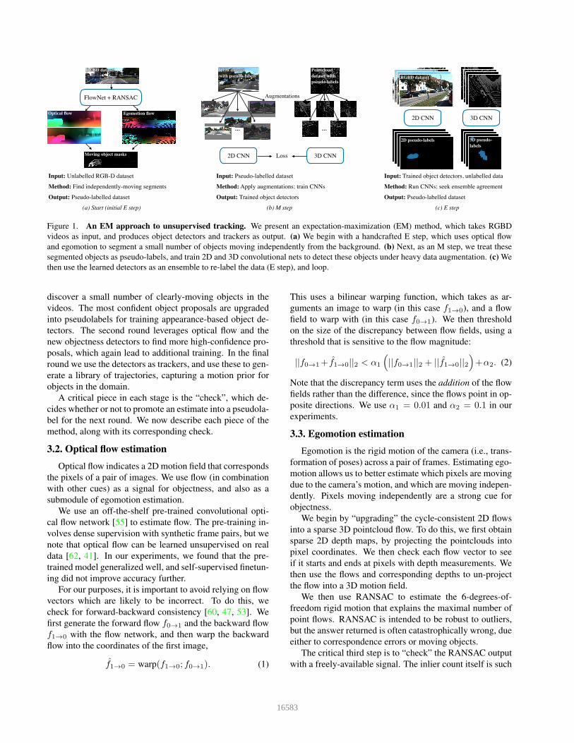
Figure 1. An EM approach to unsupervised tracking. We present an expectation-maximization (EM) method, which takes RGBD

videos as input, and produces object detectors and trackers as output. (a) We begin with a handcrafted E step, which uses optical flow

and egomotion to segment a small number of objects moving independently from the background. (b) Next, as an M step, we treat these

segmented objects as pseudo-labels, and train 2D and 3D convolutional nets to detect these objects under heavy data augmentation. (c) We

then use the learned detectors as an ensemble to re-label the data (E step), and loop.

discover a small number of clearly-moving objects in the

videos. The most confident object proposals are upgraded

into pseudolabels for training appearance-based object de-

tectors. The second round leverages optical flow and the

new objectness detectors to find more high-confidence pro-

posals, which again lead to additional training. In the final

round we use the detectors as trackers, and use these to gen-

erate a library of trajectories, capturing a motion prior for

objects in the domain.

A critical piece in each stage is the “check”, which de-

cides whether or not to promote an estimate into a pseudola-

bel for the next round. We now describe each piece of the

method, along with its corresponding check.

3.2. Optical flow estimation

Optical flow indicates a 2D motion field that corresponds

the pixels of a pair of images. We use flow (in combination

with other cues) as a signal for objectness, and also as a

submodule of egomotion estimation.

We use an off-the-shelf pre-trained convolutional opti-

cal flow network [55] to estimate flow. The pre-training in-

volves dense supervision with synthetic frame pairs, but we

note that optical flow can be learned unsupervised on real

data [62, 41]. In our experiments, we found that the pre-

trained model generalized well, and self-supervised finetun-

ing did not improve accuracy further.

For our purposes, it is important to avoid relying on flow

vectors which are likely to be incorrect. To do this, we

check for forward-backward consistency [60, 47, 53]. We

first generate the forward flow f0→1 and the backward flow

f1→0 with the flow network, and then warp the backward

flow into the coordinates of the first image,

f1→0 = warp(f1→0; f0→1). (1)

This uses a bilinear warping function, which takes as ar-

guments an image to warp (in this case f1→0), and a flow

field to warp with (in this case f0→1). We then threshold

on the size of the discrepancy between flow fields, using a

threshold that is sensitive to the flow magnitude:

||f0→1+ f1→0||2 < α1

(

||f0→1||2 + ||f1→0||2

)

+α2. (2)

Note that the discrepancy term uses the addition of the flow

fields rather than the difference, since the flows point in op-

posite directions. We use α1 = 0.01 and α2 = 0.1 in our

experiments.

3.3. Egomotion estimation

Egomotion is the rigid motion of the camera (i.e., trans-

formation of poses) across a pair of frames. Estimating ego-

motion allows us to better estimate which pixels are moving

due to the camera’s motion, and which are moving indepen-

dently. Pixels moving independently are a strong cue for

objectness.

We begin by “upgrading” the cycle-consistent 2D flows

into a sparse 3D pointcloud flow. To do this, we first obtain

sparse 2D depth maps, by projecting the pointclouds into

pixel coordinates. We then check each flow vector to see

if it starts and ends at pixels with depth measurements. We

then use the flows and corresponding depths to un-project

the flow into a 3D motion field.

We then use RANSAC to estimate the 6-degrees-of-

freedom rigid motion that explains the maximal number of

point flows. RANSAC is intended to be robust to outliers,

but the answer returned is often catastrophically wrong, due

either to correspondence errors or moving objects.

The critical third step is to “check” the RANSAC output

with a freely-available signal. The inlier count itself is such

16583

a signal, but this demands carefully tuning the threshold for

inlier counting. Instead, we enforce cycle-consistency, sim-

ilar to flow. We estimate two rigid motions with RANSAC:

once using the forward flow, and once using the backward

flow (which delivers an estimate of the inverse transform, or

backward egomotion). We then measure the inconsistency

of these results, by applying the forward and backward mo-

tion to the same pointcloud, and measuring the maximum

alignment error:

x′

0= T bw

1→0T

fw0→1

(x0) (3)

error = maxn

(||x′

0− x0||), (4)

where Tfw0→1

denotes the rotation and translation com-

puted from forward flow, which carries the pointcloud from

timestep 0 to timestep 1, T bw1→0

is the backward counterpart,

and x0 denotes the pointcloud from timestep 0.

If the maximum displacement across the entire point-

cloud is below a threshold (set to 0.25 meters), then we treat

the estimate as “correct”. In practice we find that this occurs

about 80% of the time in the KITTI dataset.

On these successful runs, we apply the egomotion to the

pointcloud to create another 3D flow field (in addition to

the one produced by upgrading the optical flow to 3D), and

we subtract these to obtain the camera-independent mo-

tion field. Independently moving objects produce high-

magnitude regions in the egomotion-stabilized motion field,

which is an excellent cue for objectness. Examples of this

are shown in Figure 1-a and Figure 2-c: note that although

real objects are highlighted by this field, some spurious

background elements are highlighted also.

In the first “round” of optimization, we proceed di-

rectly from this stage to pseudo-label generation. Using the

pseudo-labels, we train the parameters of two object detec-

tors, described next.

3.4. 2D objectness segmentation

This module takes an RGB image as input, and produces

a binary map as output. The intent of the binary map is

to estimate the likelihood that a pixel belongs to the “mov-

ing object” class. This module transfers knowledge from

the motion-based estimators into the domain of appearance,

since it learns to mimic pseudolabels that were generated

from motion alone. This is an important aspect of the over-

all model, since it allows us to identify objects of the “mov-

ing” type even when they are stationary.

We use a 50-layer ResNet [29] with a feature pyramid

[40] as the architecture, and train the last layer with a logis-

tic loss against sparse pseudo-ground-truth:

Lseg =∑

m log(1 + exp(−s · s)), (5)

where m is a mask indicating where the supervision is valid.

We experimented with and without ImageNet pretraining

(h) Box fitting,

center-surround

(a) Input RGBD

frames

(b) Optical flow,

egomotion flow

(c) Independent

motion magnitude

(d) Visibility map

(e) Unprojected 2D

object segmentation

(f) 3D object

segmentation

(heatmap)

(g) Combined

signal

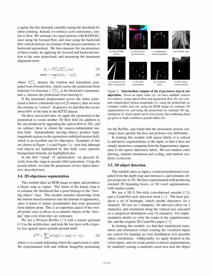
Figure 2. Intermediate outputs of the Expectation step in our

algorithm. Given an input video (a), we have multiple sources

of evidence: using optical flow and egomotion flow (b), we com-

pute independent motion magnitude (c); using the pointcloud we

compute visible area (d), using the RGB image we estimate 2D

segmentation (e), and using the pointcloud we estimate 3D seg-

mentation (f). Each signal can be error-prone, but combining them

(g) gives us high confidence pseudo-labels (h).

for the ResNet, and found that the pretrained version con-

verges more quickly but does not perform very differently.

In training this module with sparse labels, it is critical

to add heavy augmentations to the input, so that it does not

simply memorize a mapping from the happenstance appear-

ance to the sparse objectness labels. We use random color

jittering, random translation and scaling, and random syn-

thetic occlusions.

3.5. 3D object detection

This module takes as input a voxelized pointcloud (com-

puted from the depth map and intrinsics), and estimates ob-

ject proposals in 3D. We have experimented with producing

oriented 3D bounding boxes, or 3D voxel segmentations,

with similar results.

We use a 3D U-Net-style convolutional encoder [50],

and a CenterNet-style detection head [18]. The head pro-

duces a set of heatmaps, which encode objectness (in 1

channel), 3D size (in 3 channels), 3D subvoxel offset (in 3

channels), and orientation along the vertical axis (encoded

as a categorical distribution over 16 channels). For imple-

mentation details we refer the reader to the supplementary

file, and the original 2D CenterNet paper [18].

In training this module, we find that randomized trans-

lation and orientation (when creating the voxelized input)

are critical for learning an even distribution over possible

object orientations. Additionally, we apply dropout in the

voxel inputs, and we create partial occlusion augmentations

by randomly erasing a randomly-sized area near the object

16584

pseudo-label in image space, along with the 3D points that

project into that area.

3.6. Short­range tracking

To relocate a detected object over short time periods, we

use two simple techniques: hungarian matching with IoU

scores, and cross correlation with a rigid template [43]. We

find that the IoU method is sufficient in CATER, where the

motions are relatively slow. In KITTI, due to the fast mo-

tions of the objects and the additional camera motion, we

find that cross-correlation is more effective. We do this

using the features provided by the backbone of the object

detector. We simply create a template by encoding a crop

around the object, and then use this template for 3D cross

correlation against features produced in nearby frames. We

find that this is a surprisingly effective tracker despite not

handling rotations, likely because the objects do not un-

dergo large rotations under short timescales. To track for

longer periods and across occlusions, we make use of mo-

tion priors represented in a library of previously-observed

motions, described next.

3.7. Long­range tracking, with trajectory libraries

To track objects over longer time periods, we build and

use a library of motion trajectories, to act as a motion prior.

We build the library out of the successful outcomes of short-

range tracker, which typically correspond to “easy” tracking

cases, such as close-range objects will full visibility. The

key insight here is that a motion prior built from “good visi-

bility” tracklets is just as applicable to “poor visibility track-

lets”, since visibility is not a factor in objects’ motion.

To verify tracklets and upgrade them into library entries,

we check if they agree with the per-timestep cues, pro-

vided by flow, 2D segmentation, 3D object detection, and

a visibility map computed by raycasting on the pointcloud.

Specifically, we ask that a tracklet (1) obey the flow field,

and (2) travel through area that is either object-like or in-

visible. For flow agreement, we simply project the 3D ob-

ject motion to 2D and measure the inconsistency with the

2D flow in the projected region. To ensure that the trajec-

tory travels through object-like territory, we create a spa-

tiotemporal volume of objectness/visiblity cues, and trilin-

early sample in that volume at each timestep along the tra-

jectory. Each temporal slice of the volume is given by:

p = max(unproj(s) · o+ (1.0− v), 1), (6)

where unproj(s) is the 2D segmentation map unprojected to

3D (Figure 2-d), o is the 3D heatmap delivered by the object

detector (Figure 2-f), and v is the visibility map computed

through raycasting (Figure 2-d). In other words, we require

that both the 2D and 3D objectness signals agree on the

object’s presence, or that the visibility indicates the object

is in an occluded area. To evaluate a trajectory’s likelihood,

we simply take the mean of its values in the spatiotemporal

volume, and we set a stringent threshold (0.99) to prevent

erroneous tracklets from entering the library.

Once the library is built, we use it to link detections

across partial and full occlusions (where flow-based and

correlation-based tracking fails). Specifically, we orient the

library to the initial motion of an object, and then evaluate

the likelihood of all paths in the library, via the cost volume.

This is similar to a recent approach for motion planning for

self-driving vehicles [63], but here the set of possible tra-

jectories is generated from data rather than handcrafted.

3.8. Pseudo­label generation

Pseudo-label generation is what takes the model from

one round of optimization to the next. The intent is to select

the object proposals that are likely to be correct, and treat

them as ground truth for training future modules.

We take inspiration from never-ending learning architec-

tures [44], which promote an estimate into a label only if (i)

at least one module produces exceedingly-high confidence

in the estimate, or (ii) multiple modules have reasonably-

high confidence in the estimate.

The 2D and 3D modules directly produce objectness

confidences, but the motion cues need to be converted into

an objectness cue. Our strategy is inspired by classic liter-

ature on motion saliency [32]: (1) compute the magnitude

of the egomotion-stabilized 3D motion field, (2) threshold

it at a value (to mark regions with motion larger than some

speed), (3) find connected components in that binary map

(to obtain discrete regions), and (4) evaluate the center-

surround saliency of each region. Specifically, we com-

pute histograms of the motion inside the region and in the

surrounding shell, compute the chi-square distance between

the distributions, and threshold on this value [2]:

cs(θ) = χ2(h(cenθ(∆x)), h(surrθ(∆x))), (7)

where θ denotes the region being evaluated, cenθ and surrθselect points within and surrounding the region, h computes

a histogram, and ∆x denotes the egomotion-stabilized 3D

motion field.

When the trained objectness detectors are available

(i.e., on rounds after the first), we convert the egomotion-

stabilized motion field into a heatmap with exp(−λ||∆x||),and add this heatmap to the ones produced by the 2D and 3D

objectness estimators. We then proceed with thresholding,

connected components, and box fitting as normal. The only

difference is that we use a threshold that demands multiple

modules to agree: since each module produces confidences

in [0, 1], setting the threshold to any value above 2 enforces

this constraint.

16585

Figure 3. 3D object detections in CATER (top) and KITTI

(bottom). Ground-truth boxes are shown in beige and detection

results are shown in blue. IoU scores are marked alongside each

box. Results are shown in perspective RGB and bird’s-eye view.

3.9. Connection to EM

The mathematical connection to Expectation-

Maximization (EM) is not perfect, because our model

is not generative, but the mapping is quite close. Following

the terminology of Nigam et al. [45], we have:

E step: Use the current classifier to estimate the class

membership for each datapoint. In our case, use the en-

semble of handcrafted and learned modules to estimate the

objectness probability for each pixel/point.

M step: Re-estimate the classifier, using the estimated

class labels. In our case, re-optimize the parameters of the

learned components of the ensemble, using estimates pro-

duced by the ensemble as a whole (i.e., where agreement

was reached).

Note that if our classifier were a single discriminative

model, it would theoretically converge after the first M

step; using an ensemble of independent modules allows our

method to improve over rounds, since it will not converge

until all submodules produce the same labelling.

4. Experiments

We evaluate in the following datasets:

1. Synthetic RGB-D videos of tabletop scenes from

CATER [24]. CATER is a built upon CLEVR [34],

and it focuses on testing a model’s ability to do long-

term temporal reasoning. We modified the simulator

so that it can generate depth maps in addition to RGB

images, but leave all other rendering parameters un-

touched. The max number of objects is set to 10 to

make the scenes as complex as possible. Videos are

captured by 6 virtual cameras placed around the scene.

2. Real RGB-D videos of urban scenes, from the KITTI

dataset [23]. This data was collected with a sensor

platform mounted on a moving vehicle, with a hu-

man driver navigating through a variety of road types

in Germany. The data provides multiple images per

timestep; we use the “left” color camera. The dataset

provides depth in the form of LiDAR sweeps synced

to the images. We use the “tracking” subset of KITTI,

which includes 3D object labels, and approximate (but

relatively inaccurate) egomotion.

We evaluate the models on their ability to discover objects

in 3D, and track objects over time.

4.1. Baselines

For unsupervised object discovery, we use the following

baselines:

• Object-Centric Learning with Slot Attention [42].

This model trains an autoencoder with image recon-

struction loss, with soft clustering assignments as a

representational bottleneck. An iterative attention-

based update mechanism is applied when constructing

the clusters.

• MONet [9]. MONet applies a recurrent attention

mechanism that tries to explain the scene part by part.

A VAE is also trained to reconstruct the image. Since

there is no official code released, we re-implemented

using PyTorch.

• Spectral Clustering [8]. This method first extracts

dense point trajectories using optical flow, then per-

forms object segmentation by computing affinities be-

tween trajectories and then clustering.

• Discontinuity-Aware Clustering [22]. This method

also begins with dense point trajectories, but uses den-

sity discontinuities in the spectral embeddings to im-

prove the segmentation.

For tracking, we use the following baselines:

• Supervised Siamese Network [5]. This is a 3D con-

volutional net trained as a siamese object tracker. This

model produces a feature volume for the object at

t = 0, and produces feature volume for the scene at

each timestep, and then locates the object in the wider

scene by doing cross correlation at each step. The

model is supervised so that the peak of the correlation

heatmap is in the correct place.

16586

0 2 4 6 8 10 12 14 16 18Frame number

0.0

0.2

0.4

0.6

0.8

1.0

Mea

n IO

U o

ver t

ime CATER

0 2 4 6 8 10 12 14 16 18Frame number

0.0

0.2

0.4

0.6

0.8

1.0 KITTISupervised SiameseOursTracking by Colorizing

Figure 4. 3D object tracking IoU over time, in CATER and

KITTI. Tracking precision necessarily begins near 1.0 because

tracking is initialized with a real object box in frame0, and declines

over time, more drastically in KITTI than in CATER.

• Tracking by Colorizing [58]. This model learns fea-

tures through an image reconstruction task. The goal

is to colorize a grayscale image, by indexing into a

source color image with feature dot products. We up-

grade this model into a 3D tracker by associating the

learned features onto the 3D points of the object to

track, and by doing RANSAC on the point-wise cor-

respondences to estimate rigid transformations of the

target box [27].

4.2. Quantitative Results

Object discovery Our main evaluation is in Table 4.1,

where we evaluate the object proposal accuracy in mean Av-

erage Precision (mAP) at different IoU thresholds, on both

CATER and KITTI. The metrics are collected in a bird’s-

eye view (BEV) and in 2D projections (2D). We find that

our model outperforms the baselines in nearly all metrics.

Adding additional rounds of EM improves the precision at

the higher IoU thresholds. Interestingly, the learning-based

baselines, which achieve state-of-the-art results in synthetic

datasets, have near zero accuracy in KITTI. This is prob-

ably because certain assumptions in their design are vio-

lated in this data (e.g., a static-camera assumption is vio-

lated, and there is relatively little self-similarity within ob-

ject/background regions compared to CATER). See the sup-

plementary file for visualizations of the baselines’ outputs.

Object tracking Object tracking accuracy (in IoU over

time) is shown in Figure 4. To evaluate tracking, we ini-

tialize the correlation tracker with the bounding box of the

object to track.

As shown in Figure 4, the supervised model outperforms

the unsupervised ones, especially in CATER (where the

data and supervision are perfect), and by a narrower mar-

gin in KITTI. Our method can maintain relatively high IoU

over long time horizons. The IoU at frame19 is 0.34 in

KITTI and 0.7 in CATER. Our model compares favorably

to the 3D-upgraded colorization baseline.

We also input our Round2 KITTI detections to a recent

tracking-by-detection method [59], and evaluated with stan-

dard multi-object tracking metrics. We obtained sAMOTA:

0.2990; AMOTA: 0.0863; AMOTP: 0.1581. This is en-

couraging but still far behind the supervised state-of-the-

Numerical values indicate confidences, not IOUs.

Figure 5. Ablation of ensemble agreement causes divergence.

The model eventually detects objects everywhere.

art, which obtains sAMOTA: 0.9328; AMOTA: 0.4543;

AMOTP: 0.7741. Our main failure case appears to be

missed detections. We also used this tracker to compute al-

ternate results for the IoU-over-time evaluation (cf. Fig. 4):

this yields a relatively stable line around 0.44 IoU across 20

frames. Performance appears upper-bounded by the detec-

tor’s mean IoU.

Ablation on ensemble agreement Figure 5 shows what

happens when the ensemble agreement check is dropped:

the model gradually begins classifying everything as an ob-

ject (BEV mAP@.5=0.17 on Round2 instead of 0.28).

Ablation on the trajectory library Table 4.2 shows an

ablation study on the trajectory library. We report “Recall”,

which we define as the proportion of objects that are suc-

cessfully tracked by our model from the beginning of the

video to the end, where tracking success is defined by an

IoU threshold of 0.5. We also report “Precision”, which we

define as the proportion of tracklets that begin and end on

the same object. With the trajectory library, we improve

the recall from 53% to 64%, while precision drops slightly

from 94% to 91%. Qualitatively we find that the majority

of improvement is on partially and fully-occluded objects,

where strict appearance-based matching is ambiguous and

prone to failure, but where the library is a useful prior.

We present the remainder of the quantitative results in

the supplementary, showing that the tracking performance

of our model outperforms the baseline, and showing that

ablating components of our model decreases performance.

4.3. Qualitative Results

For object discovery, We show object proposals of our

model in CATER and KITTI in Figure 3. Ground-truth

boxes are shown in beige and proposed boxes are shown

in blue. Their IoU are marked near the boxes. Results are

shown on RGB image as well as bird’s-eye view. The boxes

have high recall and high precision overall; it can detect

small objects as well as separate the object that are spatially

close to each other. In KITTI, there are some false positive

results on bushes and trees because of the lack of pseudo-

label supervision there. We visualize KITTI object tracking

in Figure 6, but we encourage the reader to inspect the sup-

plementary video for clearer tracking visualizations.

16587

Method DatasetmAP@X

0.1 0.2 0.3 0.4 0.5 0.6 0.7

Slot Attention [42]CATER (2D) 0.63 0.51 0.43 0.34 0.22 0.1 0.05

KITTI (2D) 0.07 0.03 0.01 0 0 0 0

MONet [9]CATER (2D) 0.23 0.14 0.12 0.10 0.07 0.03 0.01

KITTI (2D) 0.03 0.01 0 0 0 0 0

Spectral Clustering [8]CATER (2D) 0.18 0.08 0.04 0.03 0.01 0 0

KITTI (2D) 0.08 0.03 0.02 0.02 0.01 0 0

Discontinuity

Aware Clustering [22]

CATER (2D) 0.17 0.08 0.04 0.02 0.01 0.01 0

KITTI (2D) 0.08 0.04 0.03 0.01 0 0 0

Ours

(Round1)

CATER (2D) 0.98 0.97 0.97 0.94 0.86 0.7 0.36

KITTI (2D) 0.53 0.39 0.18 0.06 0.03 0.01 0.01

CATER (BEV) 0.97 0.92 0.75 0.57 0.34 0.06 0

KITTI (BEV) 0.46 0.42 0.06 0 0 0 0

Ours

(Round2)

CATER (2D) 0.98 0.97 0.96 0.94 0.88 0.69 0.33

KITTI (2D) 0.43 0.40 0.39 0.33 0.30 0.22 0.10

CATER (BEV) 0.97 0.95 0.84 0.66 0.46 0.08 0

KITTI (BEV) 0.41 0.39 0.35 0.31 0.28 0.11 0.02

Ours

(Round3)

CATER (2D) 0.98 0.98 0.97 0.95 0.88 0.71 0.34

KITTI (2D) 0.43 0.4 0.37 0.35 0.33 0.3 0.21

CATER (BEV) 0.98 0.97 0.9 0.76 0.46 0.1 0.02

KITTI (BEV) 0.4 0.38 0.35 0.33 0.31 0.23 0.06

Table 1. Object discovery performance, in CATER and KITTI. Results are reported as mean average precision (mAP) at several IoU

threshols. Our method works best in all the metrics reported. 2D means perspective view and BEV means bird’s-eye view.

Method Recall Precision

Ours, with short-range tracker 0.53 0.94

. . . and trajectory library 0.64 0.91

Table 2. Ablations of the trajectory library, in CATER.

4.4. Limitations

The proposed method has two main limitations. Firstly,

our work assumes access to RGB-D data with accurate

depth, which excludes the method from application to gen-

eral videos (e.g., from YouTube). Second, it is unclear how

best to mine for negatives (i.e., “not a moving object”).

Right now we use a small region around each pseudo label

as negative, but it leaves the method prone to false positives

in far-away non-objects like bushes and trees.

5. Conclusion

We propose an unsupervised method for detecting and

tracking objects in unlabelled RGB-D videos. We be-

gin with a simple handcrafted technique for segmenting

independently-moving objects from the background, rely-

ing on cycle-consistent flows and RANSAC. We then train

an ensemble of 2D and 3D detectors with these segmenta-

tions, under heavy data augmentation. We then use these

detectors to re-label the dataset more densely, and return to

the training step. The ensemble agreement keeps precision

Figure 6. 3D object tracking in KITTI. IoU scores are marked

alongside each estimated box (in blue) across subsampled frames.

of the pseudo-labels high, and the data augmentations allow

recall to gradually expand. Our approach opens new av-

enues for learning object detectors from videos in arbitrary

environments, without requiring explicit object supervision.

Acknowledgements This material is based upon work

supported by US Army contract W911NF20D0002, Sony

AI, DARPA Machine Common Sense, an NSF CAREER

award, and the Air Force Office of Scientific Research un-

der award number FA9550-20-1-0423. Any opinions, find-

ings and conclusions or recommendations expressed in this

material are those of the author(s) and do not necessarily

reflect the views of the United States Army or the United

States Air Force.

16588

References

[1] Bogdan Alexe, Thomas Deselaers, and Vittorio Ferrari.

What is an object? In 2010 IEEE computer society con-

ference on computer vision and pattern recognition, pages

73–80. IEEE, 2010. 1

[2] Bogdan Alexe, Thomas Deselaers, and Vittorio Ferrari. Mea-

suring the objectness of image windows. IEEE transactions

on pattern analysis and machine intelligence, 34(11):2189–

2202, 2012. 1, 5

[3] Zeyuan Allen-Zhu and Yuanzhi Li. Towards understanding

ensemble, knowledge distillation and self-distillation in deep

learning. arXiv preprint arXiv:2012.09816, 2020. 2

[4] Dan Barnes, Will Maddern, Geoffrey Pascoe, and Ingmar

Posner. Driven to distraction: Self-supervised distractor

learning for robust monocular visual odometry in urban en-

vironments. In 2018 IEEE International Conference on

Robotics and Automation (ICRA), pages 1894–1900. IEEE,

2018. 2

[5] Luca Bertinetto, Jack Valmadre, Joao F Henriques, Andrea

Vedaldi, and Philip HS Torr. Fully-convolutional siamese

networks for object tracking. In European conference on

computer vision, pages 850–865. Springer, 2016. 6

[6] Goutam Bhat, Felix Jaremo Lawin, Martin Danelljan, An-

dreas Robinson, Michael Felsberg, Luc Van Gool, and Radu

Timofte. Learning what to learn for video object segmenta-

tion, 2020. 2

[7] Thomas Brox and Jitendra Malik. Object segmentation by

long term analysis of point trajectories. In Kostas Daniilidis,

Petros Maragos, and Nikos Paragios, editors, ECCV, pages

282–295, 2010. 2

[8] Thomas Brox and Jitendra Malik. Object segmentation by

long term analysis of point trajectories. In European confer-

ence on computer vision, pages 282–295. Springer, 2010. 6,

8

[9] Christopher P Burgess, Loic Matthey, Nicholas Watters,

Rishabh Kabra, Irina Higgins, Matt Botvinick, and Alexan-

der Lerchner. Monet: Unsupervised scene decomposition

and representation. arXiv preprint arXiv:1901.11390, 2019.

1, 2, 6, 8

[10] Andrew Carlson, Justin Betteridge, Bryan Kisiel, Burr Set-

tles, Estevam R. Hruschka, and Tom M. Mitchell. Toward

an architecture for never-ending language learning. In Pro-

ceedings of the Twenty-Fourth AAAI Conference on Artificial

Intelligence, AAAI’10, page 1306–1313. AAAI Press, 2010.

2

[11] Ting Chen, Simon Kornblith, Mohammad Norouzi, and Ge-

offrey Hinton. A simple framework for contrastive learning

of visual representations. arXiv preprint arXiv:2002.05709,

2020. 2

[12] Xinlei Chen, Abhinav Shrivastava, and Abhinav Gupta.

NEIL: Extracting visual knowledge from web data. In ICCV,

pages 1409–1416, 2013. 2

[13] Jiyu Cheng, Yuxiang Sun, and Max Q-H Meng. Improving

monocular visual slam in dynamic environments: an optical-

flow-based approach. Advanced Robotics, 33(12):576–589,

2019. 2

[14] J. Costeira and T. Kanade. A multi-body factorization

method for motion analysis. ICCV, 1995. 2

[15] Lincoln G Craton. The development of perceptual comple-

tion abilities: Infants’ perception of stationary, partially oc-

cluded objects. Child Development, 67(3):890–904, 1996.

1

[16] Antonia Creswell, Kyriacos Nikiforou, Oriol Vinyals, An-

dre Saraiva, Rishabh Kabra, Loic Matthey, Chris Burgess,

Malcolm Reynolds, Richard Tanburn, Marta Garnelo, et al.

Alignnet: Unsupervised entity alignment. arXiv preprint

arXiv:2007.08973, 2020. 2

[17] Thomas G Dietterich. Ensemble methods in machine learn-

ing. In International workshop on multiple classifier systems,

pages 1–15. Springer, 2000. 2

[18] Kaiwen Duan, Song Bai, Lingxi Xie, Honggang Qi, Qing-

ming Huang, and Qi Tian. Centernet: Keypoint triplets for

object detection. In Proceedings of the IEEE International

Conference on Computer Vision, pages 6569–6578, 2019. 4

[19] S. M. Ali Eslami, Nicolas Heess, Theophane Weber, Yuval

Tassa, David Szepesvari, koray kavukcuoglu, and Geoffrey E

Hinton. Attend, infer, repeat: Fast scene understanding with

generative models. In D. Lee, M. Sugiyama, U. Luxburg, I.

Guyon, and R. Garnett, editors, Advances in Neural Infor-

mation Processing Systems, volume 29, pages 3225–3233.

Curran Associates, Inc., 2016. 2

[20] Katerina Fragkiadaki, Pablo Arbelaez, Panna Felsen, and Ji-

tendra Malik. Learning to segment moving objects in videos.

In CVPR, June 2015. 2

[21] Katerina Fragkiadaki and Jianbo Shi. Detection free track-

ing: Exploiting motion and topology for segmenting and

tracking under entanglement. In CVPR, 2011. 1

[22] Katerina Fragkiadaki, Geng Zhang, and Jianbo Shi. Video

segmentation by tracing discontinuities in a trajectory em-

bedding. In 2012 IEEE Conference on Computer Vision and

Pattern Recognition, pages 1846–1853. IEEE, 2012. 6, 8

[23] Andreas Geiger, Philip Lenz, Christoph Stiller, and Raquel

Urtasun. Vision meets robotics: The kitti dataset. Interna-

tional Journal of Robotics Research (IJRR), 2013. 2, 6

[24] Rohit Girdhar and Deva Ramanan. CATER: A diagnostic

dataset for Compositional Actions and TEmporal Reasoning.

In ICLR, 2020. 1, 6

[25] E Bruce Goldstein. Perceiving objects and scenes: the gestalt

approach to object perception. Goldstein EB. Sensation

and Perception. 8th ed. Belmont, CA: Wadsworth Cengage

Learning, 2009. 1

[26] Klaus Greff, Raphael Lopez Kaufman, Rishabh Kabra, Nick

Watters, Christopher Burgess, Daniel Zoran, Loic Matthey,

Matthew Botvinick, and Alexander Lerchner. Multi-object

representation learning with iterative variational inference.

In International Conference on Machine Learning, pages

2424–2433. PMLR, 2019. 2

[27] Adam W Harley, Shrinidhi K Lakshmikanth, Paul Schydlo,

and Katerina Fragkiadaki. Tracking emerges by looking

around static scenes, with neural 3D mapping. In ECCV,

2020. 7

[28] Kaiming He, Haoqi Fan, Yuxin Wu, Saining Xie, and Ross

Girshick. Momentum contrast for unsupervised visual rep-

resentation learning. In CVPR, 2020. 2

16589

[29] Kaiming He, Xiangyu Zhang, Shaoqing Ren, and Jian Sun.

Deep residual learning for image recognition. In Proceed-

ings of the IEEE conference on computer vision and pattern

recognition, pages 770–778, 2016. 4

[30] Geoffrey Hinton, Oriol Vinyals, and Jeff Dean. Distill-

ing the knowledge in a neural network. arXiv preprint

arXiv:1503.02531, 2015. 1, 2

[31] Yuan-Ting Hu, Hong-Shuo Chen, Kexin Hui, Jia-Bin Huang,

and Alexander G. Schwing. Sail-vos: Semantic amodal in-

stance level video object segmentation - a synthetic dataset

and baselines. In The IEEE Conference on Computer Vision

and Pattern Recognition (CVPR), June 2019. 2

[32] Laurent Itti and Christof Koch. A saliency-based search

mechanism for overt and covert shifts of visual attention. Vi-

sion research, 40(10-12):1489–1506, 2000. 5

[33] Jindong Jiang*, Sepehr Janghorbani*, Gerard De Melo, and

Sungjin Ahn. Scalor: Generative world models with scal-

able object representations. In International Conference on

Learning Representations, 2020. 2

[34] Justin Johnson, Bharath Hariharan, Laurens van der Maaten,

Li Fei-Fei, C. Lawrence Zitnick, and Ross Girshick. Clevr:

A diagnostic dataset for compositional language and elemen-

tary visual reasoning, 2016. 1, 6

[35] Maik Keller, Damien Lefloch, Martin Lambers, Shahram

Izadi, Tim Weyrich, and Andreas Kolb. Real-time 3d re-

construction in dynamic scenes using point-based fusion.

In 2013 International Conference on 3D Vision-3DV 2013,

pages 1–8. IEEE, 2013. 2

[36] C. Kerl, J. Sturm, and D. Cremers. Dense visual SLAM for

RGB-D cameras. In IROS, 2013. 2

[37] Anna Khoreva, Rodrigo Benenson, Eddy Ilg, Thomas Brox,

and Bernt Schiele. Lucid data dreaming for object tracking.

In CVPR Workshops, 2017. 2

[38] Tejas Kulkarni, Ankush Gupta, Catalin Ionescu, Sebas-

tian Borgeaud, Malcolm Reynolds, Andrew Zisserman, and

Volodymyr Mnih. Unsupervised learning of object keypoints

for perception and control. In NeurIPS, 2019. 1

[39] Yu Li, Zhuoran Shen, and Ying Shan. Fast video object seg-

mentation using the global context module, 2020. 2

[40] Tsung-Yi Lin, Piotr Dollar, Ross Girshick, Kaiming He,

Bharath Hariharan, and Serge Belongie. Feature pyra-

mid networks for object detection. In Proceedings of the

IEEE conference on computer vision and pattern recogni-

tion, pages 2117–2125, 2017. 4

[41] Pengpeng Liu, Michael Lyu, Irwin King, and Jia Xu. Self-

low: Self-supervised learning of optical flow. In Proceed-

ings of the IEEE Conference on Computer Vision and Pattern

Recognition, pages 4571–4580, 2019. 3

[42] Francesco Locatello, Dirk Weissenborn, Thomas Un-

terthiner, Aravindh Mahendran, Georg Heigold, Jakob

Uszkoreit, Alexey Dosovitskiy, and Thomas Kipf. Object-

centric learning with slot attention. Advances in Neural In-

formation Processing Systems, 33, 2020. 2, 6, 8

[43] Lain Matthews, Takahiro Ishikawa, and Simon Baker. The

template update problem. IEEE transactions on pattern

analysis and machine intelligence, 26(6):810–815, 2004. 5

[44] Tom Mitchell, William Cohen, Estevam Hruschka, Partha

Talukdar, Bishan Yang, Justin Betteridge, Andrew Carlson,

Bhavana Dalvi, Matt Gardner, Bryan Kisiel, et al. Never-

ending learning. Communications of the ACM, 61(5):103–

115, 2018. 5

[45] Kamal Nigam, Andrew Kachites McCallum, Sebastian

Thrun, and Tom Mitchell. Text classification from labeled

and unlabeled documents using EM. Machine learning,

39(2):103–134, 2000. 1, 6

[46] P. Ochs and T. Brox. Object segmentation in video: A hi-

erarchical variational approach for turning point trajectories

into dense regions. In ICCV, 2011. 2

[47] Pan Pan, Fatih Porikli, and Dan Schonfeld. Recurrent

tracking using multifold consistency. In Proceedings of

the Eleventh IEEE International Workshop on Performance

Evaluation of Tracking and Surveillance, 2009. 3

[48] F. Perazzi, A. Khoreva, R. Benenson, B. Schiele, and A.

Sorkine-Hornung. Learning video object segmentation from

static images. In 2017 IEEE Conference on Computer Vision

and Pattern Recognition (CVPR), pages 3491–3500, 2017. 2

[49] Ilija Radosavovic, Piotr Dollar, Ross Girshick, Georgia

Gkioxari, and Kaiming He. Data distillation: Towards omni-

supervised learning. In Proceedings of the IEEE Conference

on Computer Vision and Pattern Recognition (CVPR), June

2018. 2

[50] Olaf Ronneberger, Philipp Fischer, and Thomas Brox. U-

net: Convolutional networks for biomedical image segmen-

tation. In International Conference on Medical image com-

puting and computer-assisted intervention, pages 234–241.

Springer, 2015. 4

[51] Sudeep Sarkar and Kim L Boyer. Perceptual organization

in computer vision: A review and a proposal for a classifi-

catory structure. IEEE Transactions on Systems, Man, and

Cybernetics, 23(2):382–399, 1993. 1

[52] T. Schops, J. Engel, and D. Cremers. Semi-dense visual

odometry for AR on a smartphone. In ISMAR, 2014. 2

[53] Ishwar K Sethi and Ramesh Jain. Finding trajectories of fea-

ture points in a monocular image sequence. IEEE Transac-

tions on pattern analysis and machine intelligence, 9(1):56–

73, 1987. 3

[54] Elizabeth S Spelke, J Mehler, M Garrett, and E Walker.

Perceptual knowledge of objects in infancy. In NJ: Erl-

baum Hillsdale, editor, Perspectives on mental representa-

tion, chapter 22. Erlbaum, 1982. 1

[55] Zachary Teed and Jia Deng. Raft: Recurrent all-pairs field

transforms for optical flow. In European Conference on

Computer Vision, pages 402–419. Springer, 2020. 3

[56] Josh Tobin, Rachel Fong, Alex Ray, Jonas Schneider, Woj-

ciech Zaremba, and Pieter Abbeel. Domain randomization

for transferring deep neural networks from simulation to the

real world. In 2017 IEEE/RSJ international conference on

intelligent robots and systems (IROS), pages 23–30. IEEE,

2017. 2

[57] Carlo Tomasi and Takeo Kanade. Shape and motion from

image streams under orthography: A factorization method.

Int. J. Comput. Vision, 9(2):137–154, Nov. 1992. 2

16590

[58] Carl Vondrick, Abhinav Shrivastava, Alireza Fathi, Sergio

Guadarrama, and Kevin Murphy. Tracking emerges by col-

orizing videos. In Proceedings of the European Conference

on Computer Vision (ECCV), pages 391–408, 2018. 7

[59] Xinshuo Weng, Jianren Wang, David Held, and Kris Kitani.

AB3DMOT: A Baseline for 3D Multi-Object Tracking and

New Evaluation Metrics. ECCVW, 2020. 7

[60] Hao Wu, Aswin C Sankaranarayanan, and Rama Chellappa.

In situ evaluation of tracking algorithms using time reversed

chains. In 2007 IEEE Conference on Computer Vision and

Pattern Recognition, pages 1–8. IEEE, 2007. 3

[61] Heng Yang, Jingnan Shi, and Luca Carlone. TEASER: Fast

and certifiable point cloud registration. IEEE Transactions

on Robotics, 2020. 2

[62] Jason J. Yu, Adam W. Harley, and Konstantinos G. Derpa-

nis. Back to basics: Unsupervised learning of optical flow

via brightness constancy and motion smoothness. In ECCV,

2016. 3

[63] Wenyuan Zeng, Wenjie Luo, Simon Suo, Abbas Sadat, Bin

Yang, Sergio Casas, and Raquel Urtasun. End-to-end inter-

pretable neural motion planner. In Proceedings of the IEEE

Conference on Computer Vision and Pattern Recognition,

pages 8660–8669, 2019. 5

16591