Embed Size (px)
Citation preview
Tracial state spaces of higher stable rank simpleC∗-algebras
by
Fernando de Lacerda Mortari
A thesis submitted in conformity with the requirementsfor the degree of Doctor of PhilosophyGraduate Department of Mathematics
University of Toronto
Copyright © 2009 by Fernando de Lacerda Mortari
Abstract
Tracial state spaces of higher stable rank simple C∗-algebras
Fernando de Lacerda Mortari
Doctor of Philosophy
Graduate Department of Mathematics
University of Toronto
2009
Ten years ago, J. Villadsen constructed the first examples of simple C∗-algebras with
stable rank other than one or infinity. Villadsen’s examples all had a unique tracial
state.
It is natural to ask whether examples can be found of simple C∗-algebras with higher
stable rank and more than one tracial state; by building on Villadsen’s construction, we
describe such examples that admit arbitrary tracial state spaces.
ii
Acknowledgements
I would first of all like to thank my parents, for the education they gave me, and for
all their dedication and love. I thank my entire family for their support and care, in
particular my sisters, and my nephew Arthur and niece Isabela, for bringing such joy to
my life. This is for you.
To my supervisor, Professor George A. Elliott, for all his invaluable insights, and for
showing me Mathematics under a completely new light, my most profound and sincere
thanks. Sharing his passion and dedication towards Mathematics over these past four
years has been a great honour to me.
I thank all my colleagues at the Department of Mathematics at the University of
Toronto and the Fields Institute, especially Alin Ciuperca, Alan Lai, Greg Maloney,
Leonel Robert, Barry Rowe, Luis Santiago, Aaron Tikuisis and friends from the Operator
Algebras Seminar, for all the mathematical discussions, insights, advice and knowledge
we shared. I have learned a lot from all of you.
I also thank the Department of Mathematics at the University of Toronto, the Fields
Institute, the 89 Chestnut Residence and their respective staffs for providing me with
such wonderful living and working conditions. In particular, I thank Ida Bulat for always
being so kind and helpful.
To my love, Alda, for her unrelenting support and understanding of my dream that
took me so far away and for so long, among other various reasons too numerous to
describe, my eternal gratitude; these past four years were anything but easy, on so many
levels, and you were always there for me. Thank you.
Finally, I would like to thank the CAPES Foundation and, ultimately, the people of
Brazil for trusting in me and blessing me with the means to pursue my degree. I am
deeply grateful for this honour and hope to be able to repay it in the years to come
helping shape the minds and future of our country.
iii
Contents
1 Introduction 1
2 Villadsen algebras 4
2.1 Stable and real ranks . . . . . . . . . . . . . . . . . . . . . . . . . . . . . 4
2.2 Obtaining the higher stable ranks . . . . . . . . . . . . . . . . . . . . . . 6
2.3 Constructing the algebras . . . . . . . . . . . . . . . . . . . . . . . . . . 9
3 Generalizing the construction 11
3.1 Order unit spaces, tracial states . . . . . . . . . . . . . . . . . . . . . . . 11
3.2 Generalized diagonal *-homomorphisms, Markov operators . . . . . . . . 18
3.3 The main theorem . . . . . . . . . . . . . . . . . . . . . . . . . . . . . . 21
3.4 The real rank, and further questions . . . . . . . . . . . . . . . . . . . . 32
Bibliography 35
iv
Chapter 1
Introduction
The topological stable rank for C∗-algebras was introduced by Marc A. Rieffel in [13], as
a notion of noncommutative dimension for C∗-algebras. Given a C∗-algebra A, the stable
rank of A is the least integer n such that the subset Lgn(A) of An, consisting of all the
n-tuples that generate A as a left ideal, is dense in An. If no such n exists, the stable
rank of A is defined to be infinity.
For a commutative C∗-algebra C(X), the stable rank is proportional to the covering
dimension of the spectrum X of the algebra; there are commutative C∗-algebras with
arbitrary stable rank values, including infinity. If we on the other hand look at the class
of simple C∗-algebras, the picture there was not so clear at first. While many examples
of simple C∗-algebras with stable rank one (or infinity) were known, it was not until ten
years ago that the first examples of simple C∗-algebras with stable rank other than one
or infinity were found, by Jesper Villadsen ([21]).
These Villadsen algebras can appear to be quite strange at first; they are simple, unital
and stably finite algebras with highly nontrivial K-theory, as indicated by holes present
in their K0 groups, and that came to life through an application of powerful tools from
differential topology into C∗-algebra theory. These tools were used originally by Villadsen
([20],[21]) and later by others to settle several open questions in the theory of nuclear
1
Chapter 1. Introduction 2
C∗-algebras ([15],[14],[18]), including the construction of the first counterexamples to the
strongest form of Elliott’s classification conjecture for separable amenable C∗-algebras
([19]).
Andrew Toms later produced more stably finite examples of higher stable rank simple
C∗-algebras using Villadsen’s techniques and a generalized mapping torus construction
([17]); despite the complexity of the C∗-algebras in both classes of examples, their tracial
simplices are remarkably simple: these C∗-algebras all admit a unique tracial state. It
is therefore natural to ask whether examples can be found of simple C∗-algebras with
higher stable rank and more than one tracial state (as is the case with so many classes
of simple C∗-algebras with stable rank one).
The purpose of this thesis is to settle this question affirmatively by concretely pro-
ducing examples of simple C∗-algebras with stable rank other than one and more than
one tracial state. In fact, our main result states that such C∗-algebras can have arbitrary
tracial state spaces (Theorem 3.3.2). The constructed examples constitute a generaliza-
tion of Villadsen’s class of examples in [21], and the arbitrary tracial state spaces are
obtained by an adaptation to our setting of the techniques used by Klaus Thomsen to
prove that a certain class of AI-algebras admits arbitrary tracial state spaces ([16]).
The content of this thesis is organized as follows:
In Chapter 2, we look at the notions of stable and real ranks in a little more detail,
and give a brief description of the construction of Villadsen’s algebras, as well as some of
the techniques used to obtain the higher stable ranks; this is meant to provide the reader
with a picture of the construction that will be generalized in the following chapter.
In Chapter 3, we proceed to generalize Villadsen’s construction in order to obtain
examples with more than one tracial state. In the first section we recall Thomsen’s
argument to produce his AI examples, and identify the problems in adapting his method
to Villadsen algebras; the remainder of this section, and also the second section, deal
with generalizing results of Thomsen to this new setting. The third section contains our
Chapter 1. Introduction 3
main result, Theorem 3.3.2, that shows the class of Villadsen examples can be expanded
to allow for richer structure on traces. The fourth and final section deals with estimating
the real rank for the C∗-algebras obtained, and examining some related open questions.
Chapter 2
Villadsen algebras
In this chapter we examine a class of C∗-algebras constructed by Villadsen in [21], the
first examples of simple unital stably finite C∗-algebras with stable rank other than one,
reviewing some of the technical aspects and tools necessary for their construction.
It is worth mentioning that Villadsen constructed earlier another class of simple C∗-
algebras in [20], that are also often referred to as Villadsen algebras. These were AH
algebras with stable rank one, and lots of tracial states; their interesting feature was
perforation in the K0 group, which in particular showed that there are simple AH alge-
bras that don’t have slow dimension growth. We will use the term Villadsen algebras
specifically in reference to his second class of examples.
2.1 Stable and real ranks
As stated in the introduction, given a unital C∗-algebra A and a positive integer n, one
says that the (left) stable rank of A is less than or equal to n if the subset Lgn(A) of An
consisting of all the n-tuples that generate A algebraically as a left ideal, is dense in An;
the stable rank of A is then defined to be the least such n, and denoted sr(A). If no such
n exists, the stable rank of A is defined to be infinity.
The topological stable rank was introduced by Rieffel as a noncommutative dimension
4
Chapter 2. Villadsen algebras 5
for C∗-algebras; the following theorem illustrates well the relation between the topological
stable rank and dimension, for commutative C∗-algebras.
Theorem 2.1.1. If X is a compact Hausdorff space, then
sr(C(X)) = bdim(X)/2c+ 1.
It follows from the definition of stable rank that a unital C∗-algebra has stable rank
one when its set of invertible elements is dense in the algebra. Examples of simple stable
rank one C∗-algebras include for instance the class of simple unital AH-algebras with
slow dimension growth ([7]).
Examples of simple C∗-algebras with infinite stable rank include all simple unital
purely infinite C*-algebras ([13]).
In what follows we deal with a number of homogeneous C∗-algebras of the form
p(C(X)⊗K)p, for X a compact metric space, p a projection in C(X)⊗K, and K the
algebra of compact operators on separable Hilbert space, and work with their stable
ranks; these can be calculated using the formula in the following result, that generalizes
the result above for commutative C∗-algebras, and follows from Theorem 7 of [12].
Theorem 2.1.2. Let A be a given m-homogeneous unital C∗-algebra. Then,
sr(A) = dbdim(A)/2c/me+ 1,
where A denotes the spectrum of A with its natural topology, and de, bc are the ceiling
and floor functions, respectively.
In other words, for A = p(C(X)⊗K)p as above we have
sr(A) = dbdim(X)/2c/rank(p)e+ 1.
The real rank for C∗-algebras was introduced by Brown and Pedersen in [6] and is,
unlike the stable rank, a purely C∗-algebraic invariant: given a unital C∗-algebra A, the
Chapter 2. Villadsen algebras 6
real rank of A, denoted RR(A), is the least integer k such that the set of (k + 1)-tuples
of self-adjoint elements of A that generate A as a left ideal, is dense in Ak+1sa (Asa denotes
the set of self-adjoint elements of A). If no such k exists, the real rank of A is defined to
be infinity.
The real rank also provides a notion of noncommutative dimension for C∗-algebras.
For a commutative C∗-algebra, say C(X) for X compact, the real rank is actually equal
to the dimension of X. As shown in [6], Proposition 1.2, the real rank of a C∗-algebra A
can be related to its stable rank by the inequality
RR(A) ≤ 2sr(A)− 1.
The work of Villadsen in [21] seem to suggest that, in the case of a simple C∗-algebra
A, one has RR(A) ≤ sr(A); further evidence to this is given by Theorem 3.4.2 in the
next chapter.
2.2 Obtaining the higher stable ranks
The Villadsen algebras are AH algebras presented as A = lim−→(Ai, φi), where each Ai
is composed of a single homogeneous building block, Ai = pi(C(Xi)⊗K)pi, for some
very particular choices of compact metric spaces Xi, projections pi ∈ C(Xi)⊗K, and
*-homomorphisms φi, which we will describe below.
The first key aspect of these algebras is that they do not have slow dimension growth.
Recall that an AH algebra A is said to have slow dimension growth if it can be presented
as an AH system A = lim−→(Ai, φi), with Ai = ⊕nij=1pi,j(C(Xi,j)⊗K)pi,j, such that
lim supi→∞
sup
{dim(Xi,1)
rank(pi,1), · · · , dim(Xi,ni
)
rank(pi,ni)
}= 0.
Simple AH algebras with slow dimension growth necessarily have stable rank one ([7]),
so to obtain higher stable rank examples one must consider AH systems such that the
Chapter 2. Villadsen algebras 7
dimensions of the base spaces Xi,j grow relatively fast compared to the rank of the
projections pi,j as i tends to infinity.
Given compact metric spaces X and Y , recall that a *-homomorphism
φ : Mn(C(X)) −→ Mm(C(Y ))
is said to be diagonal if n dividesm and there are continuous maps λ1, . . . , λm/n : Y −→ X
(the eigenvalue maps of φ) such that
φ(a) =
m/n⊕i=1
a ◦ λi,
for all a in Mn(C(X)). Many interesting classes of C∗-algebras can be obtained as in-
ductive limits with diagonal *-homomorphisms, such as AF algebras, Goodearl algebras,
and even the first class of Villadsen’s examples in [20], among others.
It has been shown recently by G. Elliott, T. Ho and A. Toms that arbitrary simple uni-
tal AH algebras that can be presented as an AH system with diagonal *-homomorphisms
have stable rank one ([9]). The surprising aspect of their result is that no restriction is
made on the dimension growth of the base spaces; for instance, you could have such an
inductive limit with infinite dimensional base spaces at each step (and therefore infinite
stable rank at each finite stage), but the stable rank of the limit would still drop down
to one! Therefore, more general *-homomorphisms must be considered in constructing
higher stable rank examples.
The *-homomorphisms considered by Villadsen are what we might call generalized
diagonal ; given compact metric spaces X, Y , a set of mutually orthogonal projections
p1, . . . , pn in C(Y )⊗K, and continuous maps λ1, . . . , λn : Y −→ X, a generalized diagonal
*-homomorphism φ : C(X)⊗K −→ C(Y )⊗K can be constructed as follows: let φ :
C(X) −→ C(Y )⊗K be given by
φ(f) =n∑i=1
(f ◦ λi)pi,
Chapter 2. Villadsen algebras 8
and define φ = (idC(Y )⊗α) ◦ (φ⊗idK), where α : K⊗K −→ K is some isomorphism.
If one takes the projections pi in the above definition of φ to be trivial (that is,
Murray-von Neumann equivalent to constant projections), and restricts the domain of
φ to some matrix algebra over C(X), a diagonal *-homomorphism in the usual sense is
obtained; thus, the interest in these generalized diagonal maps comes from allowing for
projections that are twisted in some way.
Given a projection p in C(X)⊗K of constant rank, for X a compact Hausdorff space,
a complex vector bundle over X can be obtained by associating to each x ∈ X the
range of the projection p(x); similarly, each complex vector bundle of constant rank over
X can be seen as a projection in C(X)⊗K. Under this correspondence, two complex
vector bundles over X are isomorphic if and only if their corresponding projections are
Murray-von Neumann equivalent. It follows in particular that a projection is trivial if
and only if its corresponding vector bundle is trivial. Vector bundles and projections will
be therefore used interchangeably from here on.
In the next section more details are given concerning how Villadsen used nontrivial
(that is, twisted) projections to obtain his higher stable rank examples. The arguments in
the proof that his algebras have stable rank higher than one rely on precisely quantifying
how twisted the projections are, in a certain sense; to do that, some algebraic topology
is required.
The Euler class of a real vector bundle ξ over a topological space X, denoted e(ξ),
is an element of the integral cohomology ring of X that provides some measure on how
twisted the bundle ξ is; it is very useful to the present purposes in the sense that it
detects whether a vector bundle has some trivial part to it. More precisely, if you add to
any vector bundle ξ a trivial vector bundle θ, the resulting vector bundle ξ ⊕ θ will have
zero Euler class.
Chapter 2. Villadsen algebras 9
2.3 Constructing the algebras
For the convenience of the reader, in this section let us briefly review the construction
of a Villadsen algebra of stable rank n+ 1 for a given positive integer n, as an inductive
limit A = lim−→(Ai, φi). All of the missing details and proofs can be found in [21].
The first algebra, A1, is given by A1 = p1(C(Dn) ⊗ K)p1 for some trivial rank one
projection p1 ∈ C(Dn) ⊗ K), and is thus isomorphic to the commutative algebra C(Dn)
of continuous, complex valued functions on the n-fold Cartesian power of the closed unit
disk in the complex plane.
The disk has dimension two and therefore the stable rank of A1 is n+1, by the results
recalled in the previous chapter. For i ≥ 1, the base space for the algebra i+ 1 is Xi+1 =
Xi × CP(ai), where CP(ai) denotes the complex projective space of complex dimension
ai, and ai is some positive integer to be determined. Define generalized diagonal *-
homomorphisms φi : C(Xi)⊗K −→ C(Xi+1)⊗K, each obtained from two eigenvalue
maps, as follows: the first is simply projection of Xi+1 onto Xi, associated with a trivial
rank one projection over Xi+1, and the second is a point evaluation to be determined,
associated with a projection isomorphic to the pull-back to Xi+1 of the universal line
bundle over CP(ai).
Set pi+1 = φi(pi); each algebra Ai is then given by Ai = pi(C(Xi)⊗K)pi, and the
connecting *-homomorphisms are obtained by restricting φi to the algebra Ai, for all i.
The integers ai are chosen so that sr(Ai) = n + 1 for all i. This can be done by
observing that the rank of the projection pi is 2i−1, and using Theorem 2.1.2. Since
inductive limits do not increase the stable rank ([13], Theorem 5.1), we have sr(A) ≤ n+1.
Finally, the point evaluations in the eigenvalue maps are chosen to ensure simplicity of
the limit algebra.
For j = 1, . . . , n, let fj ∈ C(Dn) denote the projection onto the j-th coordinate. By
construction, each projection pi+1 is the direct sum of a trivial rank one projection with
a projection that is the pull-back to Xi+1 of a vector bundle over CP(a1)× · · · × CP(ai)
Chapter 2. Villadsen algebras 10
satisfying the condition that the n-th power of its Euler class, in the integral cohomology
ring of CP(a1)× · · · × CP(ai), is nonzero. Villadsen then showed that these projections
have enough twist to ensure that the image of (f1, . . . , fn) inside Ani via the maps φj
lies at least distance 1 away from Lgn(Ai), for all i. The proof of this fact constitutes a
fascinating application of differential topology in operator algebras, and shows that the
limit algebra A must have stable rank equal to n+ 1.
Another surprising feature of these algebras is that their real ranks were estimated
by Villadsen to be very close to their stable ranks: for a Villadsen algebra of finite stable
rank n + 1 ≥ 2 like the above, its real rank is either equal to n + 1 or n. It is not yet
known which of these two possibilities actually occur; we will have more to say on this
question in the next chapter.
Chapter 3
Generalizing the construction
As observed by Villadsen in [21], all C∗-algebras in his second class of examples, described
in the previous chapter, admit a unique tracial state.
A few years later, A. Toms described in [17] another class of higher stable rank simple
C∗-algebras, using a generalized mapping torus construction. These algebras can also be
seen to admit a unique tracial state.
In this chapter we generalize Villadsen’s construction to produce examples of higher
stable rank simple C∗-algebras with more than one tracial state; an analysis of Villadsen’s
algebras reveals that, in order to try and obtain more tracial states for these algebras,
eigenvalue maps more general than the ones used by Villadsen must be introduced. This
is by itself a nontrivial task, given that the eigenvalues affect the computations on the
twist of the projections that make up the building block algebras, and these must be
carefully monitored, to ensure the stable rank doesn’t drop in the limit algebra.
Other difficulties also arise, and will be discussed in the following two sections.
3.1 Order unit spaces, tracial states
Let us begin with a brief review of certain concepts that will be used later on. Given a
compact, convex set K in a locally convex space, consider the set Aff(K) of real-valued
11
Chapter 3. Generalizing the construction 12
continuous affine functions on K. This set is an example of a complete order unit space
([1],[2]). By the category of complete order unit spaces we mean the category whose
objects are complete order unit spaces and the morphisms of which are linear, positive,
and order unit preserving maps between two such objects.
The following simple lemma will be very useful later on.
Lemma 3.1.1. Let ψ : A −→ B be a morphism in the category of complete order unit
spaces. Then, ψ is non-expansive, i.e., ‖ψ(a)‖ ≤ ‖a‖ for all a ∈ A.
Proof. This follows immediately from Proposition II.1.3 of [1], which states that a linear
map between order unit spaces is positive if and only if it is order unit preserving and
bounded with norm one.
If K is a Bauer simplex, i.e., a Choquet simplex whose set of extreme points ∂eK
is closed, then Aff(K) is isomorphic in the category of order unit spaces to the space
CR(∂eK) of real valued, continuous functions on ∂eK, the isomorphism being the map
that sends an element of Aff(K) into its restriction to the extreme boundary ∂eK.
For a compact Hausdorff space X, the simplex K of Borel probability measures on
X is an example of a Bauer simplex; its extreme boundary is composed of the Dirac
measures (that is, the measures of the form µx, x ∈ X, such that µx(Y ) is equal to either
1 or zero depending on whether x belongs to Y or not), and is homeomorphic to X (see
[1], Corollary II.4.2). Thus, in this case Aff(K) is isomorphic to CR(X).
Given a unital C∗-algebra A, we denote by T(A) the space of tracial states on A. This
space has the structure of a Choquet simplex if, for instance, A is exact (by Theorem
II.4.4 of [5] and the fact quasi-traces on exact C∗-algebras are traces, see [11]). We
can define a covariant functor from the category of unital C∗-algebras and unital *-
homomorphisms to the category of complete order unit spaces as follows: an object A of
the former is taken to Aff(T(A)), and a unital *-homomorphism φ : A −→ B is taken to
the map φ : Aff(T(A)) −→ Aff(T(B)) given by φ(g) = g ◦ φ#, for g ∈ Aff(T(A)), where
Chapter 3. Generalizing the construction 13
φ# : T(B) −→ T(A) is the map φ#(τ) = τ ◦ φ, for τ ∈ T(B).
As before, let K denote the C∗-algebra of compact operators on a separable infinite-
dimensional Hilbert space H. Given a compact Hausdorff space X and p ∈ C(X)⊗K a
projection with constant rank, the simplex of tracial states on p(C(X)⊗K)p is affinely
homeomorphic to the simplex of Borel probability measures on X; for a given Borel
probability measure µ on X, the corresponding tracial state τ on p(C(X)⊗K)p is given
by the equation
τ(a) =1
rank(p)
∫X
Tr(a(x))dµ(x),
where Tr denotes the standard unbounded trace on the C∗-algebra of bounded operators
on H.
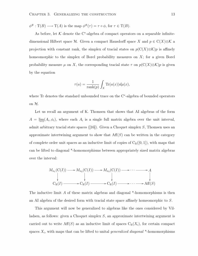
Let us recall an argument of K. Thomsen that shows that AI algebras of the form
A = lim−→(Ai, φi), where each Ai is a single full matrix algebra over the unit interval,
admit arbitrary tracial state spaces ([16]). Given a Choquet simplex S, Thomsen uses an
approximate intertwining argument to show that Aff(S) can be written in the category
of complete order unit spaces as an inductive limit of copies of CR([0, 1]), with maps that
can be lifted to diagonal *-homomorphisms between appropriately sized matrix algebras
over the interval:
Mn1(C(I)) //
��
Mn2(C(I)) //
��
Mn3(C(I)) //
��
· · · // A
��CR(I) // CR(I) // CR(I) // · · · // Aff(S)
The inductive limit A of these matrix algebras and diagonal *-homomorphisms is then
an AI algebra of the desired form with tracial state space affinely homeomorphic to S.
This argument will now be generalized to algebras like the ones considered by Vil-
ladsen, as follows: given a Choquet simplex S, an approximate intertwining argument is
carried out to write Aff(S) as an inductive limit of spaces CR(Xi), for certain compact
spaces Xi, with maps that can be lifted to unital generalized diagonal *-homomorphisms
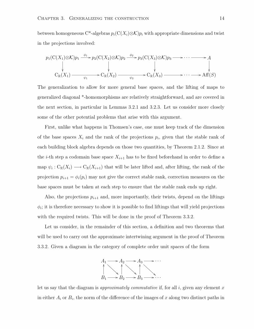
Chapter 3. Generalizing the construction 14
between homogeneous C*-algebras pi(C(Xi)⊗K)pi with appropriate dimensions and twist
in the projections involved:
p1(C(X1)⊗K)p1φ1 //
��
p2(C(X2)⊗K)p2φ2 //
��
p3(C(X3)⊗K)p3//
��
· · · // A
��CR(X1) ψ1
// CR(X2) ψ2
// CR(X3) // · · · // Aff(S)
The generalization to allow for more general base spaces, and the lifting of maps to
generalized diagonal *-homomorphisms are relatively straightforward, and are covered in
the next section, in particular in Lemmas 3.2.1 and 3.2.3. Let us consider more closely
some of the other potential problems that arise with this argument.
First, unlike what happens in Thomsen’s case, one must keep track of the dimension
of the base spaces Xi and the rank of the projections pi, given that the stable rank of
each building block algebra depends on those two quantities, by Theorem 2.1.2. Since at
the i-th step a codomain base space Xi+1 has to be fixed beforehand in order to define a
map ψi : CR(Xi) −→ CR(Xi+1) that will be later lifted and, after lifting, the rank of the
projection pi+1 = φi(pi) may not give the correct stable rank, correction measures on the
base spaces must be taken at each step to ensure that the stable rank ends up right.
Also, the projections pi+1 and, more importantly, their twists, depend on the liftings
φi; it is therefore necessary to show it is possible to find liftings that will yield projections
with the required twists. This will be done in the proof of Theorem 3.3.2.
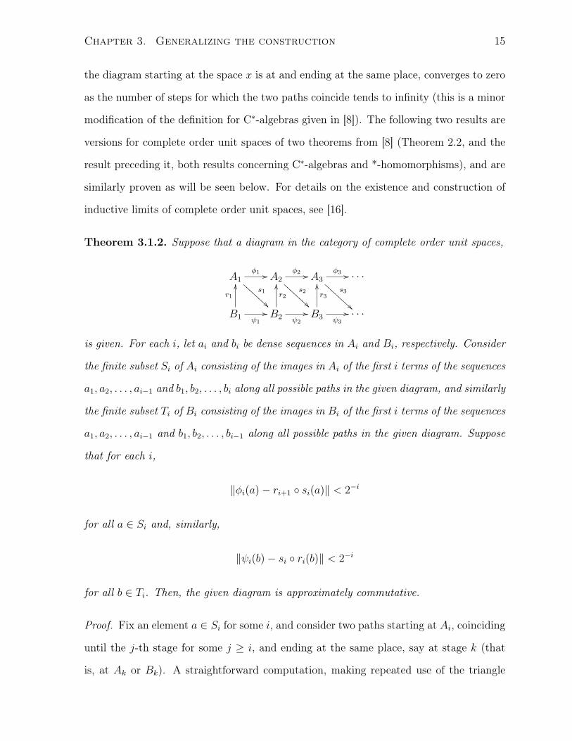
Let us consider, in the remainder of this section, a definition and two theorems that
will be used to carry out the approximate intertwining argument in the proof of Theorem
3.3.2. Given a diagram in the category of complete order unit spaces of the form
A1//
BBB
BBBB
B A2//
BBB
BBBB
B A3//
BBB
BBBB
B· · ·
B1
OO
// B2
OO
// B3
OO
// · · ·
let us say that the diagram is approximately commutative if, for all i, given any element x
in either Ai or Bi, the norm of the difference of the images of x along two distinct paths in
Chapter 3. Generalizing the construction 15
the diagram starting at the space x is at and ending at the same place, converges to zero
as the number of steps for which the two paths coincide tends to infinity (this is a minor
modification of the definition for C∗-algebras given in [8]). The following two results are
versions for complete order unit spaces of two theorems from [8] (Theorem 2.2, and the
result preceding it, both results concerning C∗-algebras and *-homomorphisms), and are
similarly proven as will be seen below. For details on the existence and construction of
inductive limits of complete order unit spaces, see [16].
Theorem 3.1.2. Suppose that a diagram in the category of complete order unit spaces,
A1φ1 //
s1
BBB
BBBB
B A2φ2 //
s2
BBB
BBBB
B A3φ3 //
s3
BBB
BBBB
B· · ·
B1
r1
OO
ψ1
// B2
r2
OO
ψ2
// B3
r3
OO
ψ3
// · · ·
is given. For each i, let ai and bi be dense sequences in Ai and Bi, respectively. Consider
the finite subset Si of Ai consisting of the images in Ai of the first i terms of the sequences
a1, a2, . . . , ai−1 and b1, b2, . . . , bi along all possible paths in the given diagram, and similarly
the finite subset Ti of Bi consisting of the images in Bi of the first i terms of the sequences
a1, a2, . . . , ai−1 and b1, b2, . . . , bi−1 along all possible paths in the given diagram. Suppose
that for each i,
‖φi(a)− ri+1 ◦ si(a)‖ < 2−i
for all a ∈ Si and, similarly,
‖ψi(b)− si ◦ ri(b)‖ < 2−i
for all b ∈ Ti. Then, the given diagram is approximately commutative.
Proof. Fix an element a ∈ Si for some i, and consider two paths starting at Ai, coinciding
until the j-th stage for some j ≥ i, and ending at the same place, say at stage k (that
is, at Ak or Bk). A straightforward computation, making repeated use of the triangle
Chapter 3. Generalizing the construction 16
inequality and Lemma 3.1.1, shows that the images of a along the two paths differ by
at most the sum of the prescribed differences at each triangle between stages j and k,
and this number goes to zero as j tends to infinity, given that the series∑∞
i=1 2−i is
summable. For instance, if we consider a ∈ A1 and the paths φ2 ◦ r2 ◦ s1 and r3 ◦ s2 ◦ φ1
starting at A1 and ending at A3, we would have (noting that φ1(a) ∈ S2)
‖φ2 ◦ r2 ◦ s1(a)− r3 ◦ s2 ◦ φ1(a)‖ ≤ ‖φ2(r2 ◦ s1(a)− φ1(a))‖+ ‖φ2(φ1(a))− r3 ◦ s2(φ1(a))‖
< ‖r2 ◦ s1(a)− φ1(a)‖+ 2−2
< 2−1 + 2−2.
The same argument holds for elements in Ti, and the density of the sequences aj, bj
ensures the desired convergence holds for arbitrary elements of Ai and Bi, completing
the proof.
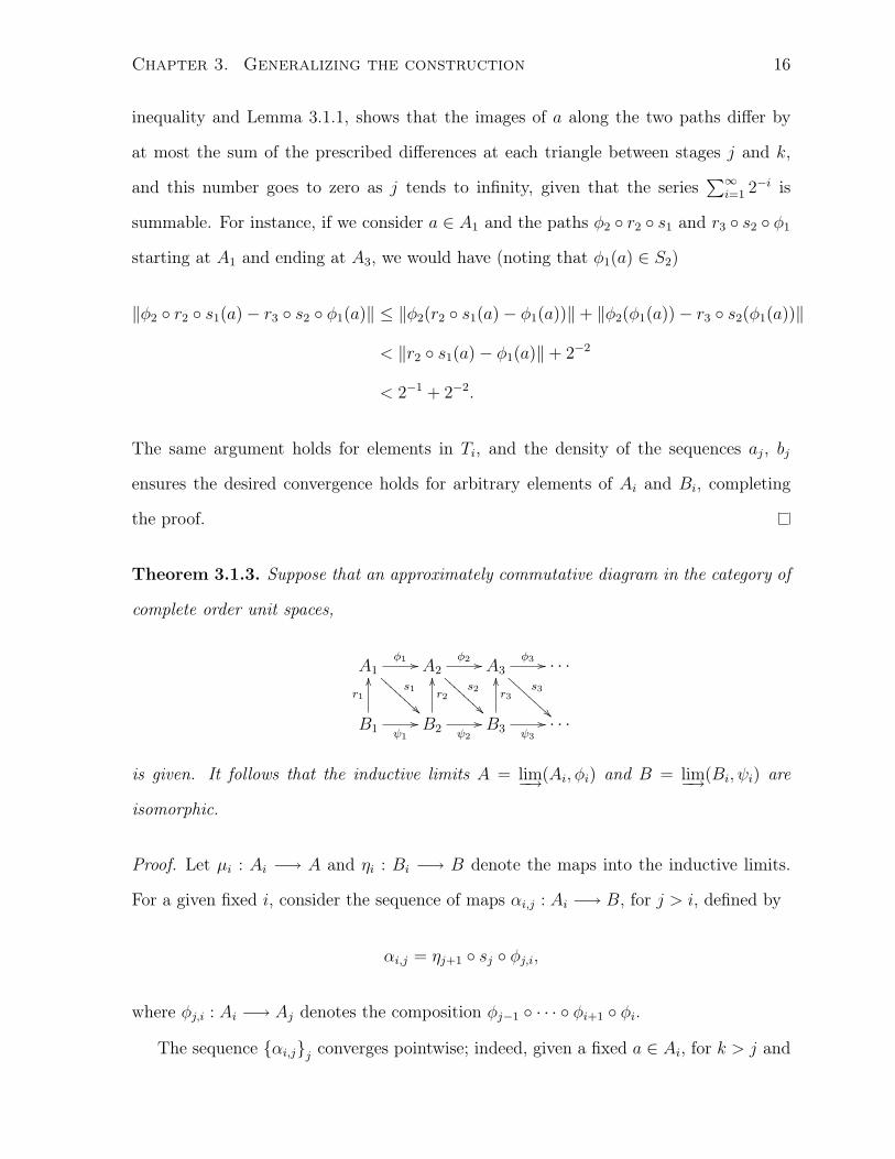
Theorem 3.1.3. Suppose that an approximately commutative diagram in the category of
complete order unit spaces,
A1φ1 //
s1
BBB
BBBB
B A2φ2 //
s2
BBB
BBBB
B A3φ3 //
s3
BBB
BBBB
B· · ·
B1
r1
OO
ψ1
// B2
r2
OO
ψ2
// B3
r3
OO
ψ3
// · · ·
is given. It follows that the inductive limits A = lim−→(Ai, φi) and B = lim−→(Bi, ψi) are
isomorphic.
Proof. Let µi : Ai −→ A and ηi : Bi −→ B denote the maps into the inductive limits.
For a given fixed i, consider the sequence of maps αi,j : Ai −→ B, for j > i, defined by
αi,j = ηj+1 ◦ sj ◦ φj,i,
where φj,i : Ai −→ Aj denotes the composition φj−1 ◦ · · · ◦ φi+1 ◦ φi.
The sequence {αi,j}j converges pointwise; indeed, given a fixed a ∈ Ai, for k > j and
Chapter 3. Generalizing the construction 17
using Lemma 3.1.1 we have the following estimate:
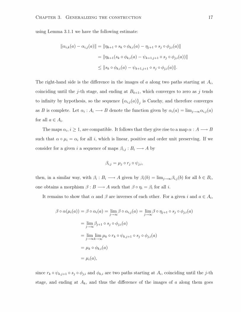
‖αi,k(a)− αi,j(a)‖ = ‖ηk+1 ◦ sk ◦ φk,i(a)− ηj+1 ◦ sj ◦ φj,i(a)‖
= ‖ηk+1(sk ◦ φk,i(a)− ψk+1,j+1 ◦ sj ◦ φj,i(a))‖
≤ ‖sk ◦ φk,i(a)− ψk+1,j+1 ◦ sj ◦ φj,i(a)‖.
The right-hand side is the difference in the images of a along two paths starting at Ai,
coinciding until the j-th stage, and ending at Bk+1, which converges to zero as j tends
to infinity by hypothesis, so the sequence {αi,j(a)}j is Cauchy, and therefore converges
as B is complete. Let αi : Ai −→ B denote the function given by αi(a) = limj→∞αi,j(a)
for all a ∈ Ai.
The maps αi, i ≥ 1, are compatible. It follows that they give rise to a map α : A −→ B
such that α ◦ µi = αi for all i, which is linear, positive and order unit preserving. If we
consider for a given i a sequence of maps βi,j : Bi −→ A by
βi,j = µj ◦ rj ◦ ψj,i,
then, in a similar way, with βi : Bi −→ A given by βi(b) = limj→∞βi,j(b) for all b ∈ Bi,
one obtains a morphism β : B −→ A such that β ◦ ηi = βi for all i.
It remains to show that α and β are inverses of each other. For a given i and a ∈ Ai,
β ◦ α(µi(a)) = β ◦ αi(a) = limj→∞
β ◦ αi,j(a) = limj→∞
β ◦ ηj+1 ◦ sj ◦ φj,i(a)
= limj→∞
βj+1 ◦ sj ◦ φj,i(a)
= limj→∞
limk→∞
µk ◦ rk ◦ ψk,j+1 ◦ sj ◦ φj,i(a)
= µk ◦ φk,i(a)
= µi(a),
since rk ◦ ψk,j+1 ◦ sj ◦ φj,i and φk,i are two paths starting at Ai, coinciding until the j-th
stage, and ending at Ak, and thus the difference of the images of a along them goes
Chapter 3. Generalizing the construction 18
to zero as j (and therefore k) tends to infinity. It follows that β ◦ α = idA; similarly,
α ◦ β = idB, whence A and B are isomorphic.
3.2 Generalized diagonal *-homomorphisms, Markov
operators
In this section we deal with the problem of lifting maps at the level of affine functions
on traces to generalized diagonal *-homomorphisms at the level of C∗-algebras. We
must of course determine what special kind of morphism is to be lifted, but first we
should perhaps see what the image φ of a generalized diagonal *-homomorphism φ via
the functor described in the previous section looks like; that’s done with the following
lemma, that generalizes a similar result of Thomsen for diagonal maps between matrix
algebras (Lemma 3.5 of [16]).
Lemma 3.2.1. Let compact Hausdorff spaces X, Y, a projection p in C(X)⊗K with
constant rank, and a unital generalized diagonal *-homomorphism
φ : (C(X)⊗K)p −→ (C(Y )⊗K)φ(p)
corresponding to a d-tuple (λi, qi)di=1, where the projections qi have constant rank 1, be
given. Then, after making the identifications of Aff(T((C(X)⊗K)p)) with CR(X) and
Aff(T((C(Y )⊗K)φ(p))) with CR(Y ), the induced map φ : CR(X) −→ CR(Y ) is given by
the formula
φ(g) =1
d
d∑i=1
g ◦ λi.
Proof. Let us begin by observing that if x, y are arbitrary points in X, Y respectively,
then the tracial states over (C(X)⊗K)p and (C(Y )⊗K)φ(p) corresponding to the Dirac
measures µx and µy are given respectively by the formulas τx(a) = 1rank(p)
Tr(a(x)), τy(b) =
Chapter 3. Generalizing the construction 19
1rank(φ(p))
Tr(b(y)). If b = φ(a), then since φ is essentially sending a to d orthogonal twisted
copies of a, namely a ◦ λi, 1 ≤ i ≤ d, we have that
τy(φ(a)) =1
rank(φ(p))Tr(φ(a)(y))
=1
rank(φ(p))
d∑i=1
Tr(a(λi(y)))
=rank(p)
rank(φ(p))
d∑i=1
τλi(y)(a).
Observing that rank(φ(p))rank(p)
= d, we therefore conclude that φ#(τy) = 1d
∑di=1 τλi(y), and the
result follows.
A linear map ω : C(X) −→ C(Y ) is called a Markov operator if it is unital and
positive. Markov operators are bounded, and they constitute a convex subset of the
space of bounded operators from C(X) to C(Y ), whose extreme boundary is given by
Hom1(C(X),C(Y )), the set of unital *-homomorphisms from C(X) to C(Y ) (see [16]).
The following theorem is a Krein-Milman type theorem for Markov operators due to
Thomsen ([16], Theorem 2.1), included here for convenience.
Theorem 3.2.2. Assume that X is path-connected. Then the closed convex hull of the
unital *-homomorphisms from C(X) to C(Y ), in the strong operator topology, is the set
of Markov operators.
The rational convex hull of Hom1(C(X),C(Y )), denoted by coQ Hom1(C(X),C(Y )),
is the set of Markov operators of the form
ω =N∑j=1
αjdωj,
where N, d, α1, . . . , αN are natural numbers satisfying∑N
j=1 αj = d and with ωj ∈
Hom1(C(X),C(Y )), 1 ≤ j ≤ N . It follows from the above theorem and the fact that Q is
dense in R that coQ Hom1(C(X),C(Y )) is dense, in the strong operator topology, in the
set of Markov operators. It is the elements in this rational convex hull that can be lifted
Chapter 3. Generalizing the construction 20
to generalized diagonal *-homomorphisms, as the following lemma shows; it generalizes
Lemma 3.6 of [16].
Lemma 3.2.3. Let compact Hausdorff spaces X, Y and ω ∈ coQ Hom1(C(X),C(Y )) be
given. If ω =∑N
j=1αj
dωj with N, d, αj, ωj as above, then there are continuous maps
λi : Y −→ X, 1 ≤ i ≤ d, satisfying the following: if q1, . . . , qd are any d mutually
orthogonal projections in C(Y )⊗K with constant rank equal to 1, and
φ : C(X)⊗K −→ C(Y )⊗K
is a generalized diagonal *-homomorphism corresponding to the d-tuple (λi, qi)di=1, then
for any nonzero projection p in C(X)⊗K with constant rank, the restricted (unital) *-
homomorphism φp : (C(X)⊗K)p −→ (C(Y )⊗K)φ(p) induced by φ satisfies φp = ω (after
making the proper identifications).
Proof. For j = 1, . . . , N , let hj : Y −→ X denote the continuous function such that the
induced unital *-homomorphism h∗j : C(X) −→ C(Y ) equals ωj (that is, for all f ∈ C(X),
we have ωj(f) = f ◦ hi).
Fix d mutually orthogonal projections q1, . . . , qd in C(Y )⊗K with constant rank equal
to 1, and define λ1, . . . , λd : Y −→ X in order by α1 copies of h1, α2 copies of h2, and so on;
let φ : C(X)⊗K −→ C(Y )⊗K be a generalized diagonal *-homomorphism corresponding
to the d-tuple (λi, qi)di=1. It now follows from Lemma 3.2.1 that, for a given g ∈ CR(X),
the restricted *-homomorphism φp satisfies
φp(g) =1
d
d∑j=1
g ◦ λj
=1
d
N∑j=1
αjg ◦ hj
=N∑j=1
αjdωj(g)
= ω(g),
completing the proof.
Chapter 3. Generalizing the construction 21
3.3 The main theorem
Suppose that M is a compact, connected and orientable differentiable manifold, and
let Dn denote the n-fold Cartesian power of the closed unit disk in the complex plane.
Let π1 : Dn ×M −→ Dn, π2 : Dn ×M −→ M denote the coordinate projections, let
aj ∈ C(Dn), 1 ≤ j ≤ n denote the projection onto the j-th coordinate, let p be a trivial
rank one projection in C(Dn ×M) ⊗ K, and let q be a projection in C(Dn ×M) ⊗ K
orthogonal to p of the form q = π∗2(η), where η is a complex vector bundle over M such
that e(η)n, the n-fold (cup) product of the Euler class e(η) of η by itself, is nonzero. Set
B = (C(Dn ×M)⊗K)p+q. The following result is due to Villadsen, and will be essential
to the proof of Theorem 3.3.2:
Theorem 3.3.1 (Villadsen ([21], Theorem 7)). Suppose that b1, . . . , bn ∈ B are such that
pbjp = (aj ◦ π1)p for each j. Then the distance from (b1, . . . , bn) to Lgn(B) is at least 1.
We are now ready for our main theorem.
Theorem 3.3.2. Let m ∈ {2, 3, . . .}∪{∞} and a non-empty metrizable Choquet simplex
S be given. Then, there exists a simple, separable, unital AH-algebra A with stable rank
m and tracial state space affinely homeomorphic to S.
Proof. By [10], Proposition 4.2, any non-empty metrizable Choquet simplex is affinely
homeomorphic to the projective limit of a sequence of finite dimensional simplices and
continuous affine maps; it follows that the space Aff(S) is isomorphic to the inductive
limit of a sequence
Rn1 θ1−→ Rn2 θ2−→ Rn3 θ3−→ · · ·
in the category of complete order unit spaces (Rn is a complete order unit space with the
usual ordering and order unit given by the element (1, 1, . . . , 1)).
Let us start with the case of finite m. Write n = m − 1, and consider the spaces
X1 = Dn and X2 = X1×CP(n), where CP(n) is the complex projective space of complex
Chapter 3. Generalizing the construction 22
dimension n. Choose n2 distinct points in X2, say b1, . . . , bn2 , and a partition of unity on
CR(X2), g1, . . . , gn2 , such that gi(bj) = δij, 1 ≤ i, j ≤ n2. Define maps s2 : Rn2 −→ CR(X2)
and r2 : CR(X2) −→ Rn2 by
s2(a1, . . . , an2) =
n2∑j=1
ajgj
r2(f) = (f(b1), . . . , f(bn2));
it can be easily verified that these maps are linear, positive, and order unit preserving
and, moreover, that s2 is injective with left inverse given by r2.
By choosing n1 distinct points in X1 and proceeding analogously as above, define
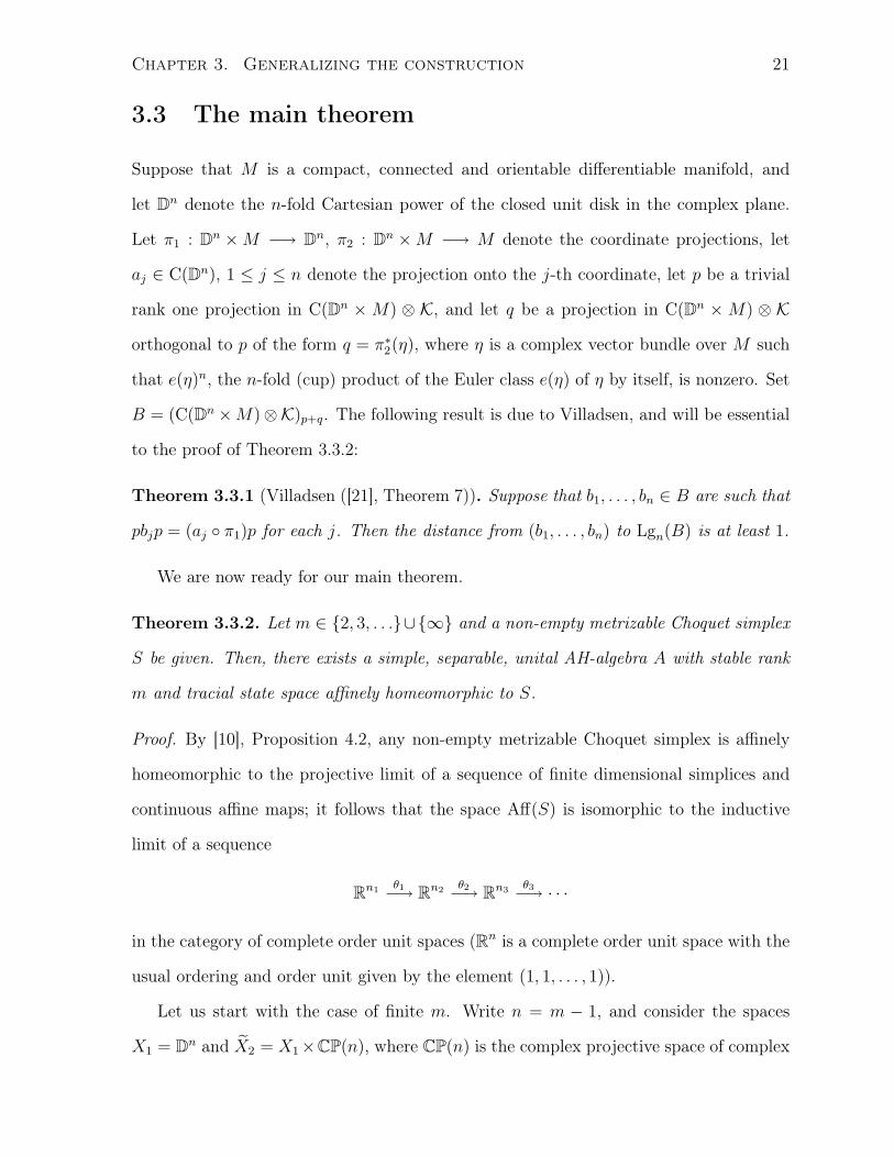
maps s1 : Rn1 −→ CR(X1) and r1 : CR(X1) −→ Rn1 with r1 as left inverse to s1. Denote
the composition map s2 ◦ θ1 ◦ r1 : CR(X1) −→ CR(X2) by ψ1. We obtain by construction
the following commutative diagram:
Rn1θ1 //
s2◦θ1%%LLLLLLLLLL Rn2
CR(X1)
r1
OO
ψ1
// CR(X2)
r2
OO
Choose a dense sequence in the closed unit ball of CR(X1) (with the supremum norm),
say f1,1, f1,2, f1,3, . . .. The map ψ1 gives rise to a Markov operator ψ′1 : C(X1) −→ C(X2)
via ψ′1(f) = ψ1(Re(f)) + iψ1(Im(f)); we can then choose γ1 ∈ coQ Hom1(C(X1),C(X2))
such that
‖ψ1(f1,1)− γ1(f1,1)‖ = ‖ψ′1(f1,1)− γ1(f1,1)‖ < 2−1.
The map γ1 is of the form
γ1 =
N1∑j=1
αj1d1
γj1,
where N1, d1, α11, . . . , α
N11 ∈ N,
∑N1
j=1 αj1 = d1, γj1 ∈ Hom1(C(X1),C(X2)), and we can
assume that d1 ≥ 23.
Chapter 3. Generalizing the construction 23
LetX2 = X1×CP(n(d1 − 1)), and denote by π the continuous projection of CP(n(d1 − 1))
onto CP(n) induced by the projection of Cn(d1−1)+1 onto Cn+1 obtained by restricting to
the first n + 1 coordinates; the map η2 := idX1 × π : X2 −→ X2 is continuous and sur-
jective, so it gives rise to a unital injective *-homomorphism η∗2 : C(X2) −→ C(X2).
Choose n2 distinct points b1, . . . , bn2 in X2 such that η2(bi) = bi, and consider the maps
r2 : CR(X2) −→ Rn2 , ψ1 : C(X1) −→ C(X2) given by
r2(f) = (f(b1), . . . , f(bn2))
ψ1 = η∗2 ◦ γ1 =
N1∑j=1
αj1d1
η∗2 ◦ γj1.
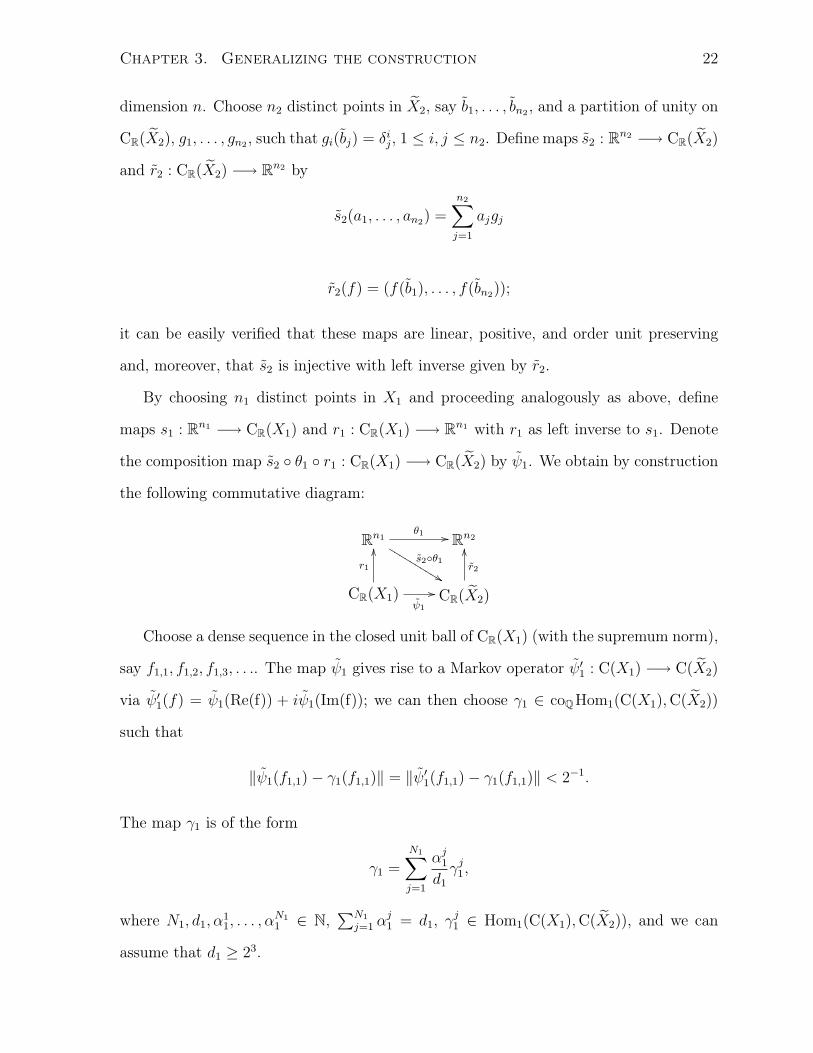
We obtain a diagram
Rn1θ1 //
η∗2◦s2◦θ1
&&LLLLLLLLLL Rn2
CR(X1)
r1
OO
ψ1
// CR(X2)
r2
OO
such that the upper triangle in the diagram is commutative, and the lower triangle
approximately commutes within 2−1 on the set S1 = {f1,1} ⊆ CR(X1). Indeed, commu-
tativity of the upper triangle follows from the fact r2 ◦ η∗2 = r2 by construction and, for
the lower triangle, we have
‖η∗2 ◦ s2 ◦ θ1 ◦ r1(f1,1)− ψ1(f1,1)‖ = ‖η∗2(ψ1(f1,1)− γ1(f1,1)
)‖ < 2−1,
using the fact η∗2 is contractive.
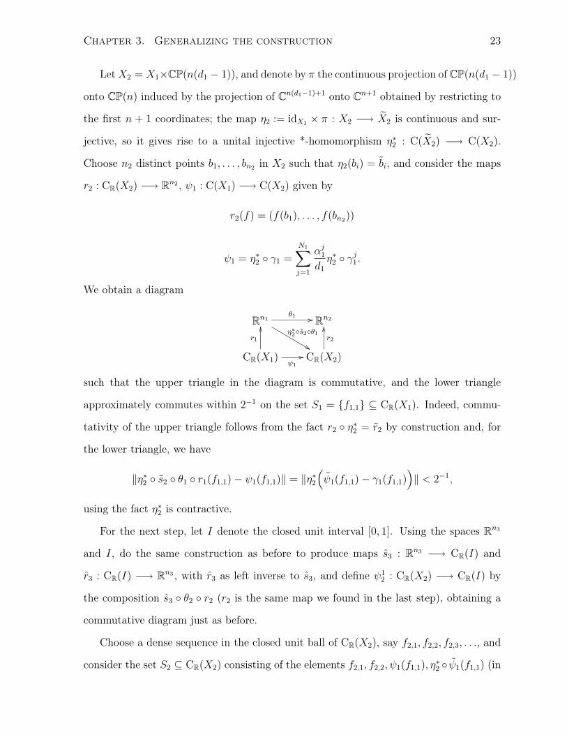
For the next step, let I denote the closed unit interval [0, 1]. Using the spaces Rn3
and I, do the same construction as before to produce maps s3 : Rn3 −→ CR(I) and
r3 : CR(I) −→ Rn3 , with r3 as left inverse to s3, and define ψ12 : CR(X2) −→ CR(I) by
the composition s3 ◦ θ2 ◦ r2 (r2 is the same map we found in the last step), obtaining a
commutative diagram just as before.
Choose a dense sequence in the closed unit ball of CR(X2), say f2,1, f2,2, f2,3, . . ., and
consider the set S2 ⊆ CR(X2) consisting of the elements f2,1, f2,2, ψ1(f1,1), η∗2 ◦ ψ1(f1,1) (in
Chapter 3. Generalizing the construction 24
other words, the first two elements of the chosen dense sequence in the closed unit ball
of CR(X2), and the images of f1,1 in CR(X2) along the two possible paths in the diagram
obtained in the last step). There is then γ12 ∈ coQ Hom1(C(X2),C(I)) such that γ1
2 and
ψ12 are close within 2−3 on the set S2; write
γ12 =
N2∑j=1
αj2d1
2
εj2,
where∑N2
j=1 αj2 = d1
2, εj2 ∈ Hom1(C(X2),C(I)), and assume that d1
2 ≥ 2√
4 = 22.
Let X3 = X2 × CP(n); by using n3 distinct points in X3, produce maps s3 : Rn3 −→
CR(X3) and r3 : CR(X3) −→ Rn3 with r3 as left inverse to s3, just as before, and denote
the composition s3 ◦ r3 : CR(I) −→ CR(X3) by ψ22.
Let S ′2 be the subset of CR(I) given by γ12(S2). Choose γ2
2 ∈ coQ Hom1(C(I),C(X3))
such that γ22 and ψ2
2 are close within 2−3 on the set S ′2. Write
γ22 =
M2∑j=1
βj2d2
2
δj2,
where∑M2
j=1 βj2 = d2
2, δj2 ∈ Hom1(C(I),C(X3)), assuming that d2
2 ≥ 22.
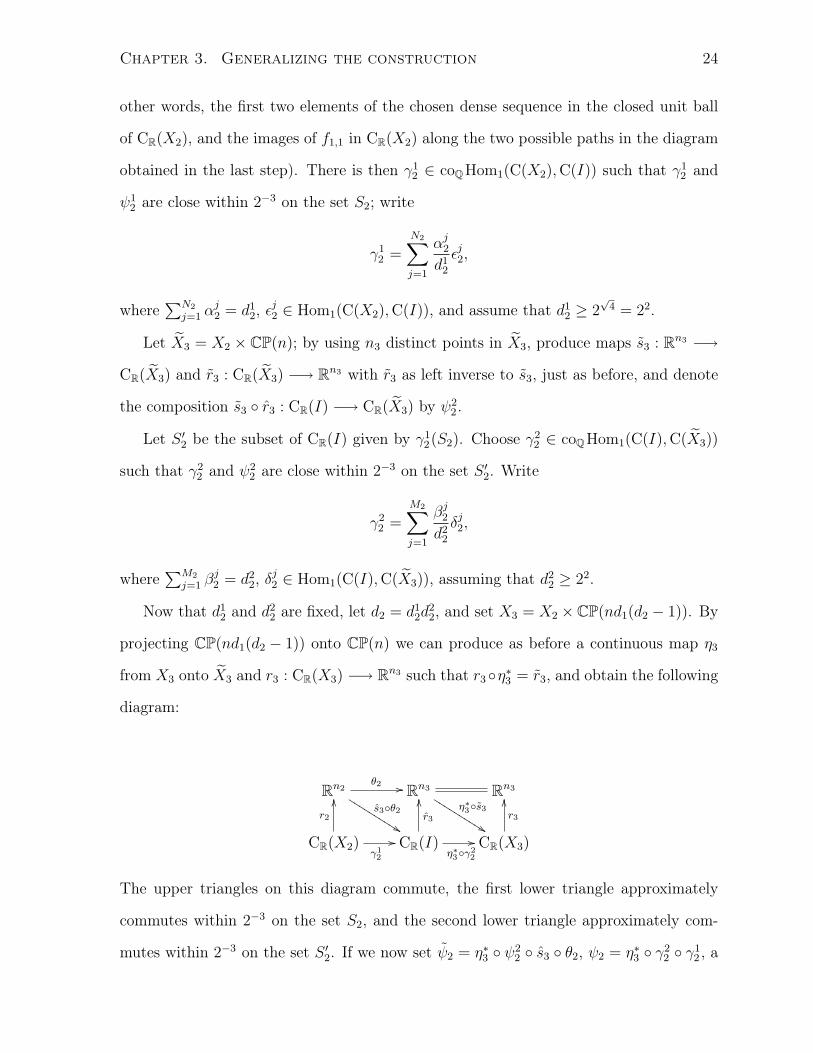
Now that d12 and d2
2 are fixed, let d2 = d12d
22, and set X3 = X2 ×CP(nd1(d2 − 1)). By
projecting CP(nd1(d2 − 1)) onto CP(n) we can produce as before a continuous map η3
from X3 onto X3 and r3 : CR(X3) −→ Rn3 such that r3◦η∗3 = r3, and obtain the following
diagram:
Rn2θ2 //
s3◦θ2
%%KKKKKKKKKK Rn3
η∗3◦s3
%%KKKKKKKKKK Rn3
CR(X2)
r2
OO
γ12
// CR(I)
r3
OO
η∗3◦γ22
// CR(X3)
r3
OO
The upper triangles on this diagram commute, the first lower triangle approximately
commutes within 2−3 on the set S2, and the second lower triangle approximately com-
mutes within 2−3 on the set S ′2. If we now set ψ2 = η∗3 ◦ ψ22 ◦ s3 ◦ θ2, ψ2 = η∗3 ◦ γ2
2 ◦ γ12 , a

Chapter 3. Generalizing the construction 25
straightforward calculation (using Lemma 3.1.1 and the fact η∗3 is non-expansive) shows
that the diagram
Rn2θ2 //
ψ2
&&LLLLLLLLLL Rn3
CR(X2)
r2
OO
ψ2
// CR(X3)
r3
OO
is commutative at the upper triangle, and approximately commutative within 2−2 on the
set S2 ⊆ CR(X2) at the lower triangle. The fact that ψ2 factors through CR(I) will be
very important later on.
The i-th step, i ≥ 3, is analogous to the second step; more precisely, use the spaces
Rni+1 and I and do the by now familiar construction to produce maps si+1 : Rni+1 −→
CR(I) and ri+1 : CR(I) −→ Rni+1 , with ri+1 as left inverse to si+1, and define ψ1i :
CR(Xi) −→ CR(I) by the composition si+1 ◦ θi ◦ ri, to obtain a commutative diagram.
After that, fix a dense sequence in the closed unit ball of CR(Xi), and set Si to be the
subset of CR(Xi) consisting of the first i elements of this sequence, together with the
images in CR(Xi) of the first i elements of all the dense sequences chosen in the previous
steps along all possible paths in the diagram
Rn1θ1 //
η∗2◦s2◦θ1
&&LLLLLLLLLL Rn2θ2 //
ψ2
&&LLLLLLLLLL Rn3θ3 //
ψ3
%%KKKKKKKKKKK · · · · · · θi−1 //
ψi−1
%%KKKKKKKKKK Rni
CR(X1)
r1
OO
ψ1
// CR(X2)
r2
OO
ψ2
// CR(X3)
r3
OO
ψ3
// · · · · · ·ψi−1
// CR(Xi)
ri
OO
Choose γ1i ∈ coQ Hom1(C(Xi),C(I)) such that γ1
i and ψ1i are close within 2−(i+1) on
the set Si, writing
γ1i =
Ni∑j=1
αjid1i
εji ,
where∑Ni
j=1 αji = d1
i , εji ∈ Hom1(C(Xi),C(I)), and such that d1
i ≥ 2√i+2.
Set Xi+1 = Xi × CP(n), construct morphisms si+1 : Rni+1 −→ CR(Xi+1) and ri+1 :
CR(Xi+1) −→ Rni+1 with ri+1 as left inverse to si+1, and let ψ2i : CR(I) −→ CR(Xi+1)
Chapter 3. Generalizing the construction 26
denote the composition si+1 ◦ ri+1. Choose γ2i ∈ coQ Hom1(C(I),C(Xi+1)) such that γ2
i
and ψ2i are close within 2−(i+1) on the set S ′i = γ1
i (Si) ⊆ CR(I), writing
γ2i =
Mi∑j=1
βjid2i
δji ,
where∑Mi
j=1 βji = d2
i and d2i ≥ 2
√i+2.
Set di = d1i d
2i , Dk =
∏kj=1 dj, and Xi+1 = Xi × CP(nDi−1(di − 1)). Just as be-
fore, there exists a continuous map ηi+1 from Xi+1 onto Xi+1, and morphisms ri+1 :
CR(Xi+1) −→ Rni+1 , si+1 : Rni+1 −→ CR(Xi+1) such that ri+1 is a left inverse to si+1 and
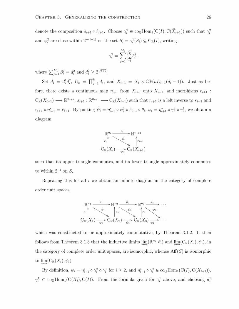
ri+1 ◦ η∗i+1 = ri+1. By putting ψi = η∗i+1 ◦ ψ2i ◦ si+1 ◦ θi, ψi = η∗i+1 ◦ γ2
i ◦ γ1i , we obtain a
diagram
Rniθi //
ψi
&&MMMMMMMMMMM Rni+1
CR(Xi)
ri
OO
ψi
// CR(Xi+1)
ri+1
OO
such that its upper triangle commutes, and its lower triangle approximately commutes
to within 2−i on Si.
Repeating this for all i we obtain an infinite diagram in the category of complete
order unit spaces,
Rn1θ1 //
ψ1
&&LLLLLLLLLL Rn2θ2 //
ψ2
&&LLLLLLLLLL Rn3θ3 //
ψ3
$$HHHHHHHHHH · · ·
CR(X1)
r1
OO
ψ1
// CR(X2)
r2
OO
ψ2
// CR(X3)
r3
OO
ψ3
// · · ·
which was constructed to be approximately commutative, by Theorem 3.1.2. It then
follows from Theorem 3.1.3 that the inductive limits lim−→(Rni , θi) and lim−→(CR(Xi), ψi), in
the category of complete order unit spaces, are isomorphic, whence Aff(S) is isomorphic
to lim−→(CR(Xi), ψi).
By definition, ψi = η∗i+1 ◦ γ2i ◦ γ1
i for i ≥ 2, and η∗i+1 ◦ γ2i ∈ coQ Hom1(C(I),C(Xi+1)),
γ1i ∈ coQ Hom1(C(Xi),C(I)). From the formula given for γ1
i above, and choosing d1i
Chapter 3. Generalizing the construction 27
orthogonal (trivial) rank one projections in C(I) ⊗ K, say ui1, . . . , uid1i, we now apply
Lemma 3.2.3 to the map γ1i to obtain continuous maps µij : I −→ Xi and a generalized
diagonal *-homomorphism
χ1i : C(Xi)⊗K −→ C(I)⊗K
associated to the d1i -tuple (µij, u
ij)j satisfying the conclusions of the lemma.
Recall that Xi+1 = Xi × CP(nci), where ci = Di−1(di − 1) (with the convention
D0 = 1); for i ≥ 1, denote by π1i+1 and π2
i+1 the projections of Xi+1 onto Xi and
CP(nci) respectively, and by Γnci the universal line bundle over CP(nci). Now, consider
the formula given for γ2i , and choose d2
i orthogonal projections in C(Xi+1) ⊗ K, say
vi+11 , . . . , vi+1
d2i, such that vi+1
1 is a trivial rank one projection and, for j ≥ 2, each vi+1j ,
when seen as a vector bundle, is isomorphic to the bundle π2∗i+1(Γnci). Apply Lemma
3.2.3 to η∗i+1 ◦ γ2i to get continuous maps λi+1
j : Xi+1 −→ I and a generalized diagonal
*-homomorphism
χ2i : C(I)⊗K −→ C(Xi+1)⊗K
associated to the d2i -tuple (λi+1
j , vi+1j )j satisfying the conclusions of the lemma.
The *-homomorphism given by the composition
χi = χ2i ◦ χ1
i : C(Xi)⊗K −→ C(Xi+1)⊗K
is also a generalized diagonal *-homomorphism, associated to a d1i d
2i -tuple (that is, a
di-tuple, if we recall di = d1i d
2i ) given by (µij ◦λi+1
k , qi+1j,k )j,k, where each qi+1
j,k is a projection
that, when seen as a vector bundle, is isomorphic to (uij ◦ λi+1k )⊗vi+1
k , which in turn is
itself isomorphic to vi+1k , since uij is a trivial rank one projection. For convenience, we
will write this di tuple as (σi+1j , qi+1
j )j; thus, for each j, σi+1j = µil ◦λi+1
k for some k, l, qi+11
is a trivial rank one projection and, for each j ≥ 2, qi+1j is isomorphic to π2∗
i+1(Γnci) (as
vector bundles).
Chapter 3. Generalizing the construction 28
The case i = 1 is easier; apply Lemma 3.2.3 to ψ1 directly to obtain χ1 associated to
the d1-tuple (σ2j , q
2j )j, where q2
1 is a trivial rank one projection and q2j is isomorphic to
π2∗2 (Γnc1) if j ≥ 2.
Let p1 be a trivial rank one projection in C(X1)⊗K and set pi+1 = χi(pi), i ≥ 1. Set
Ai = (C(Xi)⊗K)pi; if we consider the restricted (unital) *-homomorphisms χi : Ai −→
Ai+1, it then follows by functoriality and Lemma 3.2.3 that χi = ψi, since
χi = χ2i ◦ χ1
i = χ2i ◦ χ1
i = η∗i+1 ◦ γ2i ◦ γ1
i = ψi,
and χ1 = ψ1 directly from the lemma. If A is the C∗-algebra given by the inductive limit
lim−→(Ai, χi), then the above implies that Aff(T(A)) is isomorphic to Aff(S).
The algebra A is not necessarily simple; furthermore, by construction it is an AI
algebra and therefore has stable rank one. The last step of the proof consists in modifying
the algebra A to obtain a new C∗-algebra A that is simple, has stable rank n + 1, and
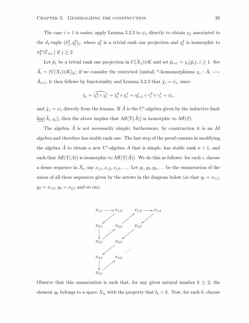
such that Aff(T(A)) is isomorphic to Aff(T(A)). We do this as follows: for each i, choose
a dense sequence in Xi, say xi,1, xi,2, xi,3, . . .. Let y1, y2, y3, . . . be the enumeration of the
union of all these sequences given by the arrows in the diagram below (so that y1 = x1,1,
y2 = x1,2, y3 = x2,1 and so on):
x1,1 // x1,2
||yyyy
yyyy
x1,3 // x1,4
||yyyy
yyyy
x2,1
��
x2,2
<<yyyyyyyyx2,3
||yyyy
yyyy
x3,1
<<yyyyyyyyx3,2
||yyyy
yyyy
x4,1
��
x4,2
...
x5,1
<<yyyyyyyy
Observe that this enumeration is such that, for any given natural number k ≥ 2, the
element yk belongs to a space Xlk with the property that lk < k. Now, for each k, choose
Chapter 3. Generalizing the construction 29
an element zk ∈ Xk such that π1lk+1 ◦ · · · ◦ π1
k−2 ◦ π1k−1(zk) = yk.
For each i, consider the generalized diagonal *-homomorphism
φi : C(Xi)⊗K −→ C(Xi+1)⊗K
corresponding to (σi+1j , qi+1
j )dij=1, obtained from χi by simply changing the eigenvalue
maps as follows: set σi+11 = π1
i+1, let σi+12 denote the constant map that takes all points
in Xi+1 into zi, and set σi+1j = σi+1
j if j = 3, . . . , di. Now, set p1 = p1, pi+1 = φi(pi) for
i ≥ 1, and set Ai = (C(Xi)⊗K)pi. The C∗-algebra A we are looking for is equal to the
inductive limit lim−→(Ai, φi).
Clearly, A is a unital AH-algebra. The point evaluations zk were chosen to ensure
that, for any a ∈ Ai, there is an index j ≥ i such that all the images of a along the
inductive sequence after the j-th stage are everywhere nonzero. This will in turn imply
in the simplicity of A by pretty much the same argument as in the proof of Proposition
2.1 of [7], and also used by Villadsen in [21].
Let us now show that Aff(T(A)) is isomorphic to Aff(T(A)): observing that, given
any i and g ∈ CR(Xi) with norm less than or equal to 1, and recalling that Lemma 3.2.1
gives us
ψi = χi =1
di
di∑j=1
g ◦ σi+1j , φi =
1
di
di∑j=1
g ◦ σi+1j ,
where d1 ≥ 23 and di = d1i d
2i ≥ 2
√i+22
√i+2 = 2i+2 if i ≥ 2, we get∥∥∥ψi(g)− φi(g)
∥∥∥ =1
di
∥∥g ◦ σi+11 + g ◦ σi+1
2 − g ◦ σi+11 − g ◦ σi+1
2
∥∥ ≤ 4
di≤ 2−i.
From this, it follows that the i-th square in the diagram below approximately commutes
to within 2−i on Si,
CR(X1)φ1 // CR(X2)
φ2 // CR(X3)φ3 // · · ·
CR(X1) ψ1
// CR(X2) ψ2
// CR(X3) ψ3
// · · ·
Chapter 3. Generalizing the construction 30
and therefore the whole diagram is approximately commutative in the category of com-
plete order unit spaces, whence their inductive limits, namely Aff(T(A)) and Aff(T(A)),
are isomorphic (again by Theorems 3.1.2 and 3.1.3). Together with the fact that Aff(T(A))
is isomorphic to Aff(S), this will in turn imply that T(A) is affinely homeomorphic to S,
as desired.
It only remains to show that the stable rank of A is n+1. Note that, by construction,
dim(X1) = 2n, rank(p1) = 1, and dim(Xi) = 2nDi−1, rank(pi) = Di−1 for i ≥ 2. Then,
since Ai is a rank(pi)-homogeneous unital C∗-algebra, by Theorem 2.1.2 its stable rank
is given by
sr(Ai) = dbdim(Ai)/2c/rank(pi)e+ 1
= dbdim(Xi)/2c/rank(pi)e+ 1
= n+ 1.
We can therefore conclude that sr(A) ≤ n + 1, and to complete the proof it is now
sufficient to show that sr(A) ≥ n+ 1 (the proof, as we shall see, is similar to the proof of
Theorem 8 of [21]).
Observe that, since φi comes from (σi+1j , qi+1
j )dij=1, as vector bundles the following
isomorphism holds:
pi+1 = φi(pi) ∼=di⊕j=1
σi+1∗j (pi)⊗ qi+1
j .
Now, if i ≥ 2, recall that each σi+1j for j ≥ 3 factors through the interval I; that is,
there are k, l such that σi+1j = µil ◦ λi+1
k with maps λi+1j : Xi+1 −→ I, µij : I −→ Xi
defined before. Therefore, σi+1∗j (pi) = λi+1∗
k (µi∗l (pi)) and, since the space I is compact
and contractible, the vector bundle µi∗l (pi) is trivial, whence σi+1∗j (pi) is a trivial vector
bundle over Xi+1 with rank equalling the rank of pi, namely Di−1. In the case j = 2,
σi+1∗2 (pi) is also trivial since σi+1
2 is a point evaluation. From this, we can conclude that,
Chapter 3. Generalizing the construction 31
for j ≥ 2,
σi+1∗j (pi)⊗ qi+1
j∼= rank(pi)q
i+1j∼= Di−1π
2∗i+1(Γnci),
where by kξ we mean the k-fold direct sum of copies of the bundle ξ and, if we recall
that σi+11 = π1∗
i+1, it follows that
pi+1∼= π1∗
i+1(pi)⊕ (di − 1)Di−1π2∗i+1(Γnci)
= π1∗i+1(pi)⊕ ciπ2∗
i+1(Γnci).
Thus, by recursion we can write
pi+1∼= ξ1 × c1Γnc1 × · · · × ciΓnci = ξ1 × ζi,
where ξ1 represents a trivial line bundle over Dn, and ζi = c1Γnc1×· · ·× ciΓnci is a vector
bundle over Mi = CP(nc1) × · · · × CP(nci) such that e(ζi)n is nonzero in the integral
cohomology ring of Mi. To see this recall that, for any positive integer k, H∗(CP(k)), the
cohomology ring of CP(k), is generated by e(Γk), with the single relation e(Γk)k+1 = 0.
Thus, e(Γncj )ncj is nonzero for all j = 1, . . . , i. That e(ζi)n is nonzero will then follow
from the Künneth formula for singular cohomology; see [20] for instance.
Now, write φi = φ1i ⊕ φ2
i , where φ1i comes from (π1
i+1, qi+11 ), and φ1
i comes from
(σi+1j , qi+1
j )j≥2. If we denote by φi,1 the composition φi−1 ◦φi−2 ◦ · · · ◦φ1 (with φ1,1 = φ1),
then pi − φ1i,1(p1) corresponds to the pull-back to Xi of the bundle ζi−1, since φ1
i,1(p1) is
the subprojection of pi that, when seen as a vector bundle, is trivial with rank one. For
j = 1, . . . , n, let aj ∈ C(Dn) be the projection onto the j-th coordinate. We have the
identity
φ1i,1(p1)φi,1(aj)φ
1i,1(p1) = φ1
i,1(aj) = (aj ◦ πi)φ1i,1(p1),
where πi denotes the projection of Xi onto X1 = Dn. Since e(ζi−1)n 6= 0, it follows from
Theorem 3.3.1 that the distance from (φi,1(a1), . . . , φi,1(an)) to Lgn(Ai) is at least one.
As a consequence, sr(A) ≥ n+ 1, whence sr(A) = n+ 1 = m, as desired.
Chapter 3. Generalizing the construction 32
In the case m is infinite, we obtain the desired algebra by doing almost the same
construction as above: we replace the spaces Xi, using instead X1 = D and, for i ≥ 1,
Xi+1 = Di(ci)2 × CP(c1)× CP(2c2)× · · · × CP(ici),
where ci = Di−1(di − 1), just as before. In particular,
Xi+1 = Dα ×Xi × CP((i+ 1)ci+1)
for some non negative integer α, so that we can define projections π1i+1 and π2
i+1 of Xi+1
onto Xi and CP((i+ 1)ci+1) respectively, and the rest of the construction is the same.
That the algebra obtained this way has infinite stable rank follows from the proof of
Theorem 12 of [21].
The C∗-algebras constructed in 3.3.2 are structurally very similar to the algebras
considered by Villadsen, and could thus rightfully be also called Villadsen algebras.
3.4 The real rank, and further questions
Let us consider the question of the real rank of the C∗algebras constructed in Theorem
3.3.2. First, the real rank for the C∗-algebras with infinite stable rank constructed in
Theorem 3.3.2 is also infinite; this follows from Theorem 13 of [21].
As mentioned in Chapter 2, Villadsen obtained an estimate for the real ranks of his
C∗-algebras with finite stable rank. The same estimates can be shown to hold for the class
of C∗-algebras constructed in Theorem 3.3.2; we need nothing more than what Villadsen
used for his estimates and, in fact, the proof follows analogously. For completeness, this
is presented below.
Recall that the real rank of an m-homogeneous C∗-algebra A is given by the following
formula ([3],[12]):
RR(A) = ddim(A)/(2m− 1)e.
Chapter 3. Generalizing the construction 33
We need the following theorem, that uses the same notation as Theorem 3.3.1; that
is, suppose that M is a compact, connected and orientable differentiable manifold. Let
π1 : Dn ×M −→ Dn, π2 : Dn ×M −→ M denote the coordinate projections, let aj ∈
C(Dn), 1 ≤ j ≤ n denote the projection onto the j-th coordinate, let p denote a trivial
rank one projection in C(Dn×M)⊗K, and let q denote a projection in C(Dn×M)⊗K
orthogonal to p of the form q = π∗2(η), where η is a complex vector bundle over M such
that e(η)n is nonzero. Set B = (C(Dn ×M)⊗K)p+q.
Theorem 3.4.1 (Villadsen ([21], Theorem 9)). Suppose that b1, . . . , bn ∈ Bsa are such
that pbjp = (Re(aj)◦π1)p for each j. Then the distance from (b1, . . . , bn) to Lgn(B)∩Bnsa
is at least 1.
Theorem 3.4.2. Let A be one of the C∗-algebras constructed in Theorem 3.3.2, and
suppose A has finite stable rank n ≥ 2. Then, its real rank is either equal to n or n− 1.
Proof. Following the notation of the proof of Theorem 3.3.2, A was written as an inductive
limit of homogeneous C∗-algebras Ai = pi(C(Xi) ⊗ K)pi, such that dim(Xi) = 2(n −
1)Di−1, rank(pi) = Di−1 for i ≥ 2. The real rank formula above then gives
RR(Ai) = ddim(A)/(2m− 1)e
= ddim(Xi)/(2rank(pi)− 1)e
= d2Di−1(n− 1)/(2Di−1 − 1)e,
which can be seen to be equal to (n − 1) + 1 = n for large enough i, and so we have
RR(A) ≤ n.
The estimate RR(A) ≥ n − 1 is obtained by the same argument as the estimate
sr(A) ≥ n in Theorem 3.3.2, only we use the real parts of the coordinate projections aj
and Theorem 3.4.1 instead of Theorem 3.3.1.
This estimate for the real rank brings up several questions, particularly if one considers
the dichotomy now established of Villadsen algebras with one, or more than one, tracial
state.
Chapter 3. Generalizing the construction 34
For instance, AI algebras have stable rank one, and therefore real rank either zero
or one; the condition of real rank zero for an AI algebra is equivalent to the algebra
admitting a unique tracial state ([16]). Therefore, for an AI algebra the real rank can be
seen to be zero or one depending on whether the algebra admits a unique tracial state,
or more than one.
A similar result holds for simple unital AH algebras with slow dimension growth
(which, as we discussed before, also have stable rank one): if such an algebra admits a
unique tracial state, then it must have real rank zero (a result that follows from [4]).
It is worth noticing that the results mentioned above for stable rank one C∗-algebras
use a particular characterization of real rank zero; namely, a C∗-algebra has real rank
zero if and only if its self-adjoint elements can be approximated arbitrarily well by self-
adjoint elements with finite spectra ([6]). Still, one can ask whether similar results hold
for Villadsen algebras. Given a Villadsen algebra with stable rank n and with a unique
(respectively, with more than one) tracial state, must its real rank be n− 1 (respectively,
n)? What about the converse statements?
These questions have resisted all attempts at solving them so far. One complication
arises from the fact that the real rank (also the stable rank, despite what the term
suggests) is far from being stable. For instance, as mentioned in the previous chapter,
one can have an inductive sequence of C∗-algebras, each with infinite real and stable
ranks, but whose inductive limit has stable rank one and real rank zero. Moreover,
even the slightest changes in the *-homomorphisms in the sequence can greatly affect
the stable and real ranks; a good example of this is seen already in the C∗-algebras of
Theorem 3.3.2: if one considers one such C∗-algebra A with stable rank n ≥ 2, then by
changing just a single eigenvalue map at each stage in the construction of A (a change
that becomes increasingly minor as one goes further along the sequence) one obtains an
AI algebra as a result. Despite this instability, it doesn’t seem unlikely at this point that
one or more of the statements above could turn out to be true.
Bibliography
[1] E. M. Alfsen. Compact convex sets and boundary integrals. Springer-Verlag, New
York, 1971. Ergebnisse der Mathematik und ihrer Grenzgebiete, Band 57.
[2] E. M. Alfsen and F. W. Shultz. State spaces of operator algebras. Mathematics:
Theory & Applications. Birkhäuser Boston Inc., Boston, MA, 2001. Basic theory,
orientations, and C∗-products.
[3] E. J. Beggs and D. E. Evans. The real rank of algebras of matrix valued functions.
Internat. J. Math., 2(2):131–138, 1991.
[4] B. Blackadar, M. Dădărlat, and M. Rørdam. The real rank of inductive limit C∗-
algebras. Math. Scand., 69(2):211–216 (1992), 1991.
[5] B. Blackadar and D. Handelman. Dimension functions and traces on C∗-algebras.
J. Funct. Anal., 45(3):297–340, 1982.
[6] L. G. Brown and G. K. Pedersen. C∗-algebras of real rank zero. J. Funct. Anal.,
99(1):131–149, 1991.
[7] M. Dădărlat, G. Nagy, A. Némethi, and C. Pasnicu. Reduction of topological stable
rank in inductive limits of C∗-algebras. Pacific J. Math., 153(2):267–276, 1992.
[8] G. A. Elliott. On the classification of C∗-algebras of real rank zero. J. Reine Angew.
Math., 443:179–219, 1993.
35
Bibliography 36
[9] G. A. Elliott, T. M. Ho, and A. Toms. A class of simple C∗-algebras with stable
rank one. J. Funct. Anal., 256(2):307–322, 2009.
[10] K. R. Goodearl. Algebraic representations of Choquet simplexes. J. Pure Appl.
Algebra, 11(1–3):111–130, 1977/78.
[11] U. Haagerup. Quasi-traces on exact C∗-algebras are traces. preprint, 1991.
[12] V. Nistor. Stable rank for a certain class of type I C∗-algebras. J. Operator Theory,
17(2):365–373, 1987.
[13] M. A. Rieffel. Dimension and stable rank in the K-theory of C∗-algebras. Proc.
London Math. Soc. (3), 46(2):301–333, 1983.
[14] M. Rørdam. Stability of C∗-algebras is not a stable property. Doc. Math., 2:375–386
(electronic), 1997.
[15] M. Rørdam. A simple C∗-algebra with a finite and an infinite projection. Acta
Math., 191(1):109–142, 2003.
[16] K. Thomsen. Inductive limits of interval algebras: the tracial state space. Amer. J.
Math., 116(3):605–620, 1994.
[17] A. Toms. On the independence of K-theory and stable rank for simple C∗-algebras.
J. Reine Angew. Math., 578:185–199, 2005.
[18] A. S. Toms. Cancellation does not imply stable rank one. Bull. London Math. Soc.,
38(6):1005–1008, 2006.
[19] A. S. Toms. On the classification problem for nuclear C∗-algebras. Ann. of Math.
(2), 167(3):1029–1044, 2008.
[20] J. Villadsen. Simple C∗-algebras with perforation. J. Funct. Anal., 154(1):110–116,
1998.
Bibliography 37
[21] J. Villadsen. On the stable rank of simple C∗-algebras. J. Amer. Math. Soc.,
12(4):1091–1102, 1999.