Embed Size (px)
Citation preview

TRACE V5.0THEORY MANUAL
Field Equations, Solution Methods,and Physical Models
Division of Risk Assessment and Special ProjectsOffice of Nuclear Regulatory ResearchU. S. Nuclear Regulatory Commission
Washington, DC 20555-0001
DRAFT

This page intentionally left blank
DRAFT

Acknowledgements
Many individuals have contributed to the NRC code consolidation effort and to this manual, inparticular. In a project of this magnitude and complexity, and given the long histories of the NRCpredecessor codes and their associated manuals (from which this manual has evolved), it is ratherdifficult to sort out and keep track of each and every individual contribution of authorship.Rather than attempt to cite individual contributors to this particular manual (and run the risk ofexcluding somebody, either past or present), we simply acknowledge all known contributors tothe TRACE code development and assessment project, in general.
Nuclear Regulatory Commission (NRC): Stephen Bajorek, Mirela Gavrilas, Chester Gingrich,James Han, Kevin Hogan, Joseph Kelly, William Krotiuk, Norman Lauben, Shanlai Lu,Christopher Murray, Frank Odar, Gene Rhee, Michael Rubin, Simon Smith, JosephStaudenmeier, Jennifer Uhle, Weidong Wang, Kent Welter, James Han, Veronica Klein, WilliamBurton, James Danna, John Jolicoeur, Sudhamay Basu, Imtiaz Madni, Shawn Marshall, AlexVelazquez, Prasad Kadambi, Dave Bessette, Margaret Bennet, Michael Salay, Andrew Ireland,William Macon, Farouk Eltawila
Advanced Systems Technology and Management (AdSTM): Yue Guan, David Ebert, DukeDu, Tong Fang, Weidong He, Millan Straka, Don Palmrose
Applied Programming Technologies (APT): Ken Jones
Applied Research Laboratory/Penn State (ARL/PSU): John Mahaffy, Mario Trujillo, MichalJelinek, Matt Lazor, Brian Hansell, Justin Watson, Michael Meholic
Information System Laboratories (ISL): Birol Aktas, Colleen Amoruso, Doug Barber, MarkBolander, Dave Caraher, Claudio Delfino, Don Fletcher, Dave Larson, Scott Lucas, GlenMortensen, Vesselin Palazov, Daniel Prelewicz, Rex Shumway, Randy Tompot, Dean Wang, JaySpore
Los Alamos National Laboratory (LANL): Brent Boyack, Skip Dearing, Joseph Durkee, JayElson, Paul Giguere, Russell Johns, James Lime, Ju-Chuan Lin, David Pimentel
Purdue University: Tom Downar, Matt Miller, Jun Gan, Han Joo, Yunlin Xu, TomaszKozlowski, Doek Jung Lee
DRAFT
iii

TRACE V4.160
Universidad Politecnica de Madrid: Roberto Herrero
Korean Nuclear Fuel Co: Jae Hoon Jeong
Korean Institute of Nuclear Safety: Chang Wook Huh, Ahn Dong Shin
DRAFT
iv

TRACE V5.0
Preface....................................................................................................xvOverview of TRACE ...............................................................................................................xv
TRACE Characteristics......................................................................................................... xvii
Multi-Dimensional Fluid Dynamics ............................................................................... xvii
Non-homogeneous, Non-equilibrium Modeling............................................................. xvii
Flow-Regime-Dependent Constitutive Equation Package ............................................. xvii
Comprehensive Heat Transfer Capability...................................................................... xviii
Component and Functional Modularity ......................................................................... xviii
Physical Phenomena Considered ......................................................................................... xviii
Limitations on Use................................................................................................................. xix
Intended Audience ...................................................................................................................xx
Organization of This Manual ................................................................................................. xxi
Reporting Code Errors ........................................................................................................... xxi
Conventions Used in This Manual........................................................................................ xxii
1: Field Equations ...................................................................................1Nomenclature.............................................................................................................................2
Fluid Field Equations.................................................................................................................6
Rearrangement of Equations for Numerical Solution........................................................14
Noncondensable Gas..........................................................................................................16
Liquid Solute......................................................................................................................17
Application Specific Usage of these Equations .......................................................................18
1-D Equations ....................................................................................................................18
Pseudo 2-D Flow ...............................................................................................................20
3-D Equations ....................................................................................................................21
Basic Finite-Volume Approximations to the Flow Equations .................................................21
Time Level Selection .........................................................................................................32
Basics of the Semi-Implicit Method ..................................................................................35
Enhancements to the Semi-Implicit Method .....................................................................37
Semi-Implicit Method Adapted to Two-Phase Flow .........................................................39
Basics of the SETS Method ...............................................................................................43
Enhancements to the SETS Method ..................................................................................46
The SETS Method Adapted to Two-Phase Flow...............................................................48
DRAFT
v

TRACE V5.0
3D Finite-Difference Methods.................................................................................................58
Modifications to the Basic Equation Set..................................................................................66
Conserving Convected Momentum .........................................................................................67
Reversible and Irreversible Form Losses...........................................................................71
Special Cases .....................................................................................................................71
References................................................................................................................................75
2: Solution Methods...............................................................................77Nomenclature...........................................................................................................................77
Overall Solution Strategy.........................................................................................................79
Basic Solution Methodology ...................................................................................................80
Solution of the 1D Stabilizer Motion Equations................................................................80
Solving the SETS Semi-Implicit Step................................................................................83
Solution of the SETS Stabilizer Mass and Energy Equations ...........................................88
Final Solution for a New-Time Void Fraction ...................................................................88
Considerations for 3D Solutions..............................................................................................90
The Capacitance Matrix Method .............................................................................................93
Water Packing ..........................................................................................................................96
3: Heat Conduction Equations..............................................................99Nomenclature...........................................................................................................................99
Governing Equations .............................................................................................................101
Coupling of Thermal Hydraulics with the Reactor Structure ................................................102
Cylindrical Wall Heat Conduction.........................................................................................105
Slab and Rod Heat Conduction..............................................................................................106
The Lumped-Parameter Solution.....................................................................................107
The Semi-Implicit Calculation.........................................................................................108
The Fully Implicit Calculation.........................................................................................112
Fine-Mesh Algorithm. .....................................................................................................115
References..............................................................................................................................118
4: Drag Models.....................................................................................119Nomenclature.........................................................................................................................119
Interfacial Drag ......................................................................................................................123
DRAFT
vi

TRACE V5.0
Pre-CHF Interfacial Drag Models....................................................................................124
Stratified Flow Interfacial Drag Models ..........................................................................148
Post-CHF Interfacial Drag Models ..................................................................................157
Wall Drag ...............................................................................................................................170
Single-Phase Friction Factor............................................................................................171
Pre-CHF Regimes: Two-Phase Multiplier .......................................................................173
Horizontal Stratified Flow Model ....................................................................................182
Post-CHF Flow Regimes .................................................................................................184
References..............................................................................................................................187
5: Interfacial Heat Transfer Models ...................................................193Nomenclature.........................................................................................................................193
Introduction............................................................................................................................197
Pre-CHF Interfacial Heat Transfer Models............................................................................200
Bubbly Flow Regime .......................................................................................................200
Cap Bubble/Slug Flow Regime .......................................................................................204
Modifications for Subcooled Boiling ..............................................................................207
Interfacial Heat Transfer Models for the Annular/Mist Flow Regime ............................208
Interpolation Region ........................................................................................................215
Flashing Model ................................................................................................................216
Stratified Flow Interfacial Heat Transfer Models ..................................................................216
Transition to Non-Stratified Flow....................................................................................219
Post-CHF Interfacial Heat Transfer Models ..........................................................................219
Inverted Annular ..............................................................................................................220
Inverted Slug....................................................................................................................224
Dispersed Flow ................................................................................................................226
Interpolation Region ........................................................................................................228
Transition to Pre-CHF Regimes.......................................................................................229
Non-Condensable Gas Effects ...............................................................................................229
Default Model for Condensation .....................................................................................230
Special Model for Film Condensation .............................................................................232
Model for Evaporation.....................................................................................................238
References..............................................................................................................................240
DRAFT
vii

TRACE V5.0
6: Wall Heat Transfer Models .............................................................245Nomenclature.........................................................................................................................245
Introduction............................................................................................................................250
Pre-CHF Heat Transfer ..........................................................................................................252
Single-Phase Liquid Convection .....................................................................................252
Two-Phase Forced Convection ........................................................................................263
Onset of Nucleate Boiling................................................................................................267
Nucleate Boiling ..............................................................................................................271
Subcooled Boiling Model ................................................................................................278
Critical Heat Flux...................................................................................................................282
AECL-IPPE CHF Table...................................................................................................284
CISE-GE Critical Quality ................................................................................................292
Biasi Critical Quality .......................................................................................................293
Minimum Film Boiling Temperature.....................................................................................295
Post-CHF Heat Transfer.........................................................................................................302
Transition Boiling ............................................................................................................302
Inverted Annular Film Boiling ........................................................................................308
Dispersed Flow Film Boiling...........................................................................................316
Inverted Slug Film Boiling ..............................................................................................336
Condensation Heat Transfer...................................................................................................338
Film Condensation...........................................................................................................338
Dropwise Condensation ...................................................................................................346
Non-Condensible Gas Effects..........................................................................................347
References..............................................................................................................................351
7: Flow Process Models.......................................................................359Nomenclature.........................................................................................................................359
Critical Flow ..........................................................................................................................362
Subcooled Liquid .............................................................................................................363
Two-Phase, Two-Component Fluid .................................................................................367
Single-Phase Vapor ..........................................................................................................373
Transition Regions ...........................................................................................................373
Cell-Center Momentum-Solution Velocities ...................................................................374
DRAFT
viii

TRACE V5.0
New-Time Choking Velocities.........................................................................................374
Determining the Sound Speed .........................................................................................375
Countercurrent Flow ..............................................................................................................376
CCFL in the 3D VESSEL................................................................................................376
The Model........................................................................................................................377
Input Scheme ...................................................................................................................378
Level Tracking .......................................................................................................................379
Level Tracking Method....................................................................................................380
Modifications To The Field Equations ............................................................................382
Mass and Energy Equations.............................................................................................382
Momentum Equations......................................................................................................385
Corrections to Evaluation of the Closure Models............................................................388
Interfacial Drag ................................................................................................................388
Interfacial Heat and Mass Transfer..................................................................................390
Numerical Experiments .........................................................................................................392
Fill and Drain Test ...........................................................................................................392
Oscillating Manometer ....................................................................................................396
Expulsion of Superheated Steam by Subcooled Water ....................................................404
Summary of the Simulations............................................................................................412
Offtake Model ........................................................................................................................412
Form Loss Models .................................................................................................................416
Abrupt Expansion ............................................................................................................421
Abrupt Contraction ..........................................................................................................422
Thin-Plate Orifice ............................................................................................................424
Models as Coded..............................................................................................................425
References..............................................................................................................................427
8: Fuel Rod Models..............................................................................431Nomenclature.........................................................................................................................431
Nuclear Fuel Mixed-Oxide Properties ...................................................................................434
Fuel Density .....................................................................................................................434
Specific Heat....................................................................................................................435
Fuel Thermal Conductivity ..............................................................................................436
DRAFT
ix

TRACE V5.0
Fuel Spectral Emissivity ..................................................................................................437
Fuel Rod Gap Gas Properties.................................................................................................438
Zircaloy Cladding Properties .................................................................................................441
Cladding Density .............................................................................................................441
Cladding Specific Heat ....................................................................................................442
Cladding Thermal Conductivity ......................................................................................443
Cladding Spectral Emissivity...........................................................................................444
Fuel-Cladding Gap Conductance...........................................................................................445
Fuel - Cladding Gap Dimension ......................................................................................446
Metal - Water Reaction ..........................................................................................................449
References..............................................................................................................................450
9: Reactor-Core Power Models ...........................................................453Nomenclature.........................................................................................................................454
Partitioning of the Core Power into the Heat-Conduction Mesh...........................................458
Power Evaluation and Reactor Kinetics ................................................................................467
Point-Reactor Kinetics .....................................................................................................467
Default Data for the Delayed-Neutron Groups................................................................469
Default Data for the Decay-Heat Groups.........................................................................470
Fission Power History......................................................................................................471
Reactivity Feedback.........................................................................................................471
Solution of the Point-Reactor Kinetics ............................................................................480
Conclusions Regarding the Reactor-Core Power Model .......................................................487
References..............................................................................................................................488
10:Special Component Models ............................................................491Nomenclature.........................................................................................................................491
PUMP Component .................................................................................................................496
Pump Governing Equations .............................................................................................496
Pump Head Modeling ......................................................................................................498
Pump Torque Modeling ...................................................................................................501
Pump Speed .....................................................................................................................502
Pump Friction Heating.....................................................................................................503
DRAFT
x
TRACE V5.0
PRIZER Component ..............................................................................................................504
Collapsed Liquid Level....................................................................................................505
Heater/Sprays...................................................................................................................506
SEPD Component ..................................................................................................................507
Definitions .......................................................................................................................510
Conceptual Structure of the SEPD Component ...............................................................511
Assumptions.....................................................................................................................511
Fundamental Analytical Model .......................................................................................512
Mechanistic Separator Modeling .....................................................................................517
Dryer Modeling................................................................................................................525
JETP Component ...................................................................................................................527
References..............................................................................................................................533
11:Fluid Properties ..............................................................................535Nomenclature.........................................................................................................................535
Thermodynamic Properties....................................................................................................536
Saturation Properties........................................................................................................537
Liquid Properties..............................................................................................................547
Steam Properties ..............................................................................................................551
Noncondensable Gas (Air, Hydrogen, or Helium) Properties .........................................558
Steam-Gas Mixture Properties .........................................................................................561
Transport Properties...............................................................................................................561
Latent Heat of Vaporization .............................................................................................562
Constant-Pressure Specific Heat......................................................................................562
Fluid Viscosity .................................................................................................................564
Fluid Thermal Conductivity.............................................................................................569
Surface Tension................................................................................................................571
Liquid Solute Properties ........................................................................................................572
Model Description ...........................................................................................................572
Verification.............................................................................................................................574
Verification of Boron Solubility Model ...........................................................................580
References..............................................................................................................................581
DRAFT
xi

TRACE V5.0
12:Structural Material Properties .......................................................583Nomenclature.........................................................................................................................583
Electrical Fuel-Rod Insulator (BN) Properties ......................................................................584
Density .............................................................................................................................584
Specific Heat....................................................................................................................584
Thermal Conductivity ......................................................................................................584
Spectral Emissivity ..........................................................................................................585
Electrical Fuel-Rod Heater-Coil (Constantan) Properties .....................................................585
Density .............................................................................................................................585
Specific Heat....................................................................................................................585
Thermal Conductivity ......................................................................................................585
Spectral Emissivity ..........................................................................................................585
Structural Material Properties ................................................................................................585
References..............................................................................................................................591
A: Quasi-Steady Assumption and Averaging Operators ....................593Nomenclature.........................................................................................................................593
Introduction............................................................................................................................595
Averagers and Limiters Arising from Temporal-Averager Considerations ...........................598
Variations in the Application of Temporal Averagers and Limiters ......................................599
Spatial-Averaging Operator ...................................................................................................600
Validity of the Quasi-Steady Assumption..............................................................................601
Concluding Remarks..............................................................................................................606
References..............................................................................................................................606
B: Finite Volume Equations.................................................................609Nomenclature.........................................................................................................................609
Approximation of the Momentum Equations ........................................................................613
Special Cases for Side Junction Flow....................................................................................623
Flow Out a Side Junction.................................................................................................624
Side Junction Inflow, Splitting in the Main Leg ..............................................................625
C: Critical Flow Model: Computational Details .................................627Nomenclature.........................................................................................................................627
DRAFT
xii

TRACE V5.0
Determining the Sound Speed ...............................................................................................629
Isentropic Expansion of Ideal Gas ...................................................................................629
L/D £ 1.5 or Noncondensable Gas Present in Two-Phase Flow at Cell Center...............630
L/D < 1.5 or Only Superheated Vapor Phase, or Only Subcooled-Liquid Phase Present at Cell Center .......................................................................................................................637
Model as Coded .....................................................................................................................648
Initial Calculations ...........................................................................................................648
Determination of Choking Velocities Using the Appropriate Model ..............................649
New-Time Choking Velocities.........................................................................................656
Second-Pass for Velocity Derivatives..............................................................................657
D:Tee Offtake Model: Computational Details ....................................659Nomenclature.........................................................................................................................659
Offtake Model Computational Sequence...............................................................................660
Upward Offtake ...............................................................................................................661
Side-Oriented Offtake......................................................................................................664
Gas Entrainment Scenario ...............................................................................................666
Downward Offtake...........................................................................................................669
DRAFT
xiii

TRACE V5.0
DRAFT
xiv
Preface
Advanced computing plays a critical role in the design, licensing and operation of nuclear powerplants. The modern nuclear reactor system operates at a level of sophistication whereby humanreasoning and simple theoretical models are simply not capable of bringing to light fullunderstanding of a system's response to some proposed perturbation, and yet, there is an inherentneed to acquire such understanding. Over the last 30 years or so, there has been a concerted efforton the part of the power utilities, the U. S. Nuclear Regulatory Commission (USNRC), andforeign organizations to develop advanced computational tools for simulating reactor systembehavior during real and hypothetical transient scenarios. The lessons learned from simulationscarried out with these tools help form the basis for decisions made concerning plant design,operation, and safety.
The TRAC/RELAP Advanced Computational Engine (TRACE - formerly called TRAC-M) is thelatest in a series of advanced, best-estimate reactor systems codes developed by the U.S. NuclearRegulatory Commission for analyzing transient and steady-state neutronic-thermal-hydraulicbehavior in light water reactors. It is the product of a long term effort to combine the capabilitiesof the NRC’s four main systems codes (TRAC-P, TRAC-B, RELAP5 and RAMONA) into onemodernized computational tool..
This manual is one of three manuals that comprise the basic TRACE documentation set. Theother two are the Users’ Manual and Developmental Assessment Manual.
Overview of TRACETRACE has been designed to perform best-estimate analyses of loss-of-coolant accidents(LOCAs), operational transients, and other accident scenarios in pressurized light-water reactors(PWRs) and boiling light-water reactors (BWRs). It can also model phenomena occuring inexperimental facilities designed to simulate transients in reactor systems. Models used includemultidimensional two-phase flow, nonequilibrium thermo-dynamics, generalized heat transfer,reflood, level tracking, and reactor kinetics. Automatic steady-state and dump/restart capabilitiesare also provided.
The partial differential equations that describe two-phase flow and heat transfer are solved usingfinite volume numerical methods. The heat-transfer equations are evaluated using a semi-implicit
DRAFT
xv
TRACE V5.0
time-differencing technique. The fluid-dynamics equations in the spatial one-dimensional (1D),and three-dimensional (3D) components use, by default, a multi-step time-differencing procedurethat allows the material Courant-limit condition to be exceeded. A more straightforward semi-implicit time-differencing method is also available, should the user demand it. The finite-difference equations for hydrodynamic phenomena form a system of coupled, nonlinear equationsthat are solved by the Newton-Raphson iteration method. The resulting linearized equations aresolved by direct matrix inversion. For the 1D network matrix, this is done by a direct full-matrixsolver; for the multiple-vessel matrix, this is done by the capacitance-matrix method using a directbanded-matrix solver.
TRACE takes a component-based approach to modeling a reactor system. Each physical piece ofequipment in a flow loop can be represented as some type of component, and each component canbe further nodalized into some number of physical volumes (also called cells) over which thefluid, conduction, and kinetics equations are averaged. The number of reactor components in theproblem and the manner in which they are coupled is arbitrary. There is no built-in limit for thenumber of components or volumes that can be modeled; the size of a problem is theoretically onlylimited by the available computer memory. Reactor hydraulic components in TRACE includePIPEs, PLENUMs, PRIZERs (pressurizers), CHANs (BWR fuel channels), PUMPs, JETPs (jetpumps), SEPDs (separators), TEEs, TURBs (turbines), HEATRs (feedwater heaters), CONTANs(containment), VALVEs, and VESSELs (with associated internals). HTSTR (heat structure) andREPEAT-HTSTR components modeling fuel elements or heated walls in the reactor system areavailable to compute two-dimensional conduction and surface-convection heat transfer inCartesian or cylindrical geometries. POWER components are available as a means for deliveringenergy to the fluid via the HTSTR or hydraulic component walls. FLPOWER (fluid power)components are capable of delivering energy directly to the fluid (such as might happen in wastetransmutation facilities). RADENC (radiation enclosures) components may be used to simulateradiation heat transfer between multiple arbitrary surfaces. FILL and BREAK components areused to apply the desired coolant-flow and pressure boundary conditions, respectively, in thereactor system to perform steady-state and transient calculations. EXTERIOR components areavailable to facilitate the development of input models designed to exploit TRACE’s parallelexecution features.
The code’s computer execution time is highly problem dependent and is a function of the totalnumber of mesh cells, the maximum allowable timestep size, and the rate of change of theneutronic and thermal-hydraulic phenomena being evaluated. The stability-enhancing two-step(SETS) numerics in hydraulic components allows the material Courant limit to be exceeded. Thisallows very large time steps to be used in slow transients. This, in turn, can lead to significantspeedups in simulations (one or two orders of magnitude) of slow-developing accidents andoperational transients.
While we do not wish to overstate the performance of the numerical techniques incorporated inTRACE, we believe that the current schemes demonstrate exceptional stability and robustnessthat will serve adequately in codes like TRACE for years to come. However, the models andcorrelations in the code can have a significant impact on the speed of a calculation; they can (andfrequently do) affect adversely the time-step size and the number of iterations used. Because ofthe impact on the speed of the calculation and because the models and correlations greatly affect
DRAFT
xvi
TRACE V5.0
the accuracy of the results, the area of model/correlation development may result in significantimprovements in overall code performance.
TRACE CharacteristicsSome distinguishing characteristics of the code are summarized below.
Multi-Dimensional Fluid Dynamics
A 3D (x, y, z) Cartesian- and/or (r, θ, z) cylindrical-geometry flow calculation can be simulatedwithin the reactor vessel or other other reactor components where 3D phenomena take place. All3D components, such as Reactor Water Storage Tank, where 3D phenomena are modeled, arenamed VESSEL although they may not have any relationship with the reactor vessel. Flowswithin a coolant loop are usually modeled in one dimension using PIPE and TEE components.The combination of 1D and 3D components allows an accurate modeling of complex flownetworks as well as local multidimensional flows. This is important in determining emergencycore coolant (ECC) downcomer penetration during blowdown, refill, and reflood periods of aLOCA. The mathematical framework exists to directly treat multidimensional plenum- and core-flow effects, and upper-plenum pool formation and core penetration during reflood.
Non-homogeneous, Non-equilibrium Modeling
A full two-fluid (six-equation) hydrodynamic model evaluates gas-liquid flow, thereby allowingimportant phenomena such as countercurrent flow to be simulated explicitly. A stratified-flowregime has been added to the 1D hydrodynamics; a seventh field equation (mass balance)describes a noncondensable gas field; and an eigh1th field equation tracks dissolved solute in theliquid field that can plated out on surfaces when solubility in the liquid is exceeded.
Flow-Regime-Dependent Constitutive Equation Package
The thermal-hydraulic equations describe the transfer of mass, energy, and momentum betweenthe steam-liquid phases and the interaction of these phases with heat flow from the modeledstructures. Because these interactions are dependent on the flow topology, a flow-regime-dependent constitutive-equation package has been incorporated into the code. Assessmentcalculations performed to date indicate that many flow conditions can be calculated accuratelywith this package.
DRAFT
xvii
TRACE V5.0
Comprehensive Heat Transfer Capability
TRACE can perform detailed heat-transfer analyses of the vessel and the loop components.Included is a 2D (r,z) treatment of conduction heat transfer within metal structures. Heatconduction with dynamic fine-mesh rezoning during reflood simulates the heat transfercharacteristics of quench fronts. Heat transfer from the fuel rods and other structures is calculatedusing flow-regime-dependent heat transfer coefficients (HTC) obtained from a generalizedboiling curve based on a combination of local conditions and history effects. Inner- and/or outer-surface convection heat-transfer and a tabular or point-reactor kinetics with reactivity feedbackvolumetric power source can be modeled. One-dimensional or three-dimensional reactor kineticscapabilities are possible through coupling with the Purdue Advanced Reactor Core Simulator(PARCS) program.
Component and Functional Modularity
The TRACE code is completely modular by component. The components in a calculation arespecified through input data; available components allow the user to model virtually any PWR orBWR design or experimental configuration. Thus, TRACE has great versatility in its range ofapplications. This feature also allows component modules to be improved, modified, or addedwithout disturbing the remainder of the code. TRACE component modules currently includeBREAKs, FILLs, CHANs, CONTANs, EXTERIORs, FLPOWERs, HEATRs, HTSTRs, JETPs,POWERs, PIPEs, PLENUMs, PRIZERs, PUMPs, RADENCs, REPEAT-HTSTRs, SEPDs,TEEs, TURBs, VALVEs, and VESSELs with associated internals (downcomer, lower plenum,reactor core, and upper plenum).
The TRACE program is also modular by function; that is, the major aspects of the calculations areperformed in separate modules. For example, the basic 1D hydrodynamics solution algorithm,the wall-temperature field solution algorithm, heat transfer coefficient (HTC) selection, and otherfunctions are performed in separate sets of routines that can be accessed by all componentmodules. This modularity allows the code to be upgraded readily with minimal effort andminimal potential for error as improved correlations and test information become available.
Physical Phenomena ConsideredAs part of the detailed modeling in TRACE, the code can simulate physical phenomena that areimportant in large-break and small-break LOCA analyses, such as:
1) ECC downcomer penetration and bypass, including the effects of countercurrent flow and hot walls;
2) lower-plenum refill with entrainment and phase-separation effects;
3) bottom-reflood and falling-film quench fronts;
DRAFT
xviii
TRACE V5.0
4) multidimensional flow patterns in the reactor-core and plenum regions;
5) pool formation and countercurrent flow at the upper-core support-plate (UCSP) region;
6) pool formation in the upper plenum;
7) steam binding;
8) water level tracking,
9) average-rod and hot-rod cladding-temperature histories;
10) alternate ECC injection systems, including hot-leg and upper-head injection;
11) direct injection of subcooled ECC water, without artificial mixing zones;
12) critical flow (choking);
13) liquid carryover during reflood;
14) metal-water reaction;
15) water-hammer pack and stretch effects;
16) wall friction losses;
17) horizontally stratified flow, including reflux cooling,
18) gas or liquid separator modeling;
19) noncondensable-gas effects on evaporation and condensation;
20) dissolved-solute tracking in liquid flow;
21) reactivity-feedback effects on reactor-core power kinetics;
22) two-phase bottom, side, and top offtake flow of a tee side channel; and reversible and irreversible form-loss flow effects on the pressure distribution
Limitations on UseAs a general rule, computational codes like TRACE are really only applicable within theirassessment range. TRACE has been qualified to analyze the ESBWR design as well asconventional PWR and BWR large and small break LOCAs (excluding B&W designs). At thispoint, assessment has not been officially performed for BWR stability analysis, or otheroperational transients.
The TRACE code is not appropriate for modeling situations in which transfer of momentum playsan important role at a localized level. For example, TRACE makes no attempt to capture, indetail, the fluid dynamics in a pipe branch or plenum, or flows in which the radial velocity profileacross the pipe is not flat.
DRAFT
xix
TRACE V5.0
The TRACE code is not appropriate for transients in which there are large changing asymmetriesin the reactor-core power such as would occur in a control-rod-ejection transient unless it is usedin conjunction with the PARCS spatial kinetics module. In TRACE, neutronics are evaluated ona core-wide basis by a point-reactor kinetics model with reactivity feedback, and the spatiallylocal neutronic response associated with the ejection of a single control rod cannot be modeled.
The typical system model cannot be applied directly to those transients in which one expects toobserve thermal stratification of the liquid phase in the 1D components. The VESSEL componentcan resolve the thermal stratification of liquid only within the modeling of its multidimensionalnoding when horizontal stratification is not perfect.
The TRACE field equations have been derived assuming that viscous shear stresses are negligible(to a first-order approximation) and explicit turbulence modeling is not coupled to theconservation equations (although turbulence effects can be accounted for with specializedengineering models for specific situations). Thus, TRACE should not be employed to modelthose scenarios where the viscous stresses are comparable to, or larger than, the wall (and/orinterfacial, if applicable) shear stresses. For example, TRACE is incapable of modelingcirculation patterns within a large open region, regardless of the choice of mesh size.
TRACE does not evaluate the stress/strain effect of temperature gradients in structures. Theeffect of fuel-rod gas-gap closure due to thermal expansion or material swelling is not modeledexplicitly. TRACE can be useful as a support to other, more detailed, analysis tools in resolvingquestions such as pressurized thermal shock.
The TRACE field equations are derived such that viscous heating terms within the fluid isgenerally ignored. A special model is, however, available within the PUMP component toaccount for direct heating of fluid by the pump rotor.
Approximations in the wall and interface heat flux terms prevent accurate calculations of suchphenomena as collapse of a steam bubble blocking natural circulation through a B&W candy-cane, or of the details of steam condensation at the water surface in an AP1000 core makeup tank.
Intended AudienceThis document is not intended to serve as a textbook on thermal-hydraulic phenomena ormodeling. We do assume that the reader has been educated in the area of two-phase flow.Instead, it is intended to describe the underlying theory at such a level that scientists and engineersnot closely involved in the development of TRACE can review the documentation and gainsufficient confidence that TRACE is adequate for its intended purpose. Along these lines, thisdocument provides a baseline against which to measure the adequacy of the current models andcorrelations and a tool to help prioritize future experiment and development activities. We havedone our best to ensure that discussions are kept at a level that precludes the need to introducecode-specific implementation details like subroutine or variable names.
DRAFT
xx
TRACE V5.0
We have also written this document for the TRACE code user who desires to understand thereasons behind the qualitative and quantitative nature of the comparisons between calculatedresults and data; to determine the applicability of the code to particular facilities and/or transients;or to determine the appropriateness of calculated results, with or without data to support thecalculations. The definition of code user includes anyone who is involved in running the code orin analyzing its calculated results. Some chapters, particulary those that discuss the componentand flow-process models, do presume some knowledge of the general TRACE modelingapproach and its nomenclature (i.e. component names, global input variables that control overallcode behavior, etc), such as might be gained from a quick read of the User’s Manual.
Individuals involved in the development of TRACE (or similar codes) should find the informationcontained in this document useful because it provides insight into the many problems associatedwith closure and demonstrates methodologies for obtaining continuity at the boundaries amongcorrelation sets that, because of their mathematical forms and different databases, are inherentlydiscontinuous. This document provides one example of how one could select correlations andmodels and define logic to link them into a coherent system to describe, in conjunction with thefield equations, a large variety of thermal-hydraulic conditions and transients. Even within thefield of reactor safety in the United States other, similar calculational tools exist (e.g. RELAP5,COBRA/TRAC, TRAC-BWR, TRAC-PWR, CATHARE, RETRAN) in which differentobjectives, constraints, and histories have led to different choices for solution strategies, models,and correlations.
Organization of This ManualThis document is designed to serve as the resource for understanding the mathematical modelsthat the code uses, how they are solved, and their limitations. In particular, it discusses the two-phase flow equations, their transformation into finite volume methods, the overall solutionprocess, the heat conduction equations, the core power and fuel rod models, and the variousconstitutive models and closure relationships employed (without necessarily delving into the low-level details of how they were developed).
Reporting Code ErrorsIt is vitally important that the USNRC receive feedback from the TRACE user community. Tothat end, we have established a support website at http://www.nrccodes.com. It contains theTRACEZilla bug tracking system, latest documentation, a list of the updates currently waiting tobe integrated into the main development trunk (called the HoldingBin), and the recent buildhistory showing what changes have been made, when, and by whom. Access to the TRACE-specific areas of the site are password-protected. Details for obtaining access are provided on thepublic portion of the site.
DRAFT
xxi

TRACE V5.0
Conventions Used in This ManualIn general. items appearing in this manual use the Times New Roman font. Sometimes, text isgiven a special appearance to set it apart from the regular text. Here’s how they look (colored textwill, of course, not appear colored when printed in black and white)
ALL CAPS
Used for TRACE component names and input variable names
BOLD RED, ALL CAPS
Used for TRACE variable identifiers in the component card tables (column 2)
Bold Italic
Used for chapter and section headings
Bold Blue
Used for TRACE card titles, note headings, table headings, cross references
Plain Red
Used for XTV graphics variable names
Bold
Used for filenames, pathnames, table titles, headings for some tables, and AcGrace dialog box names
Italic
Used for references to a website URL and AcGrace menu items
Fixed Width Courier
Used to indicate user input, command lines, file listings, or otherwise, any text that you would see or type on the screen
Note – This icon represents a Note. It is used to emphasize various informational messages that might be of interest to the reader. This is some invisible text - its sole purpose is to make the paragraph a little longer so that the bottom line will extend below the icon.
Warning – This icon represents a Warning. It is used to emphazize important information that you need to be aware of while you are working with TRACE. This is some invisible text - its sole purpose is to make the paragraph a little longer so that the bottom line will extend below the icon.
!
DRAFT
xxii

TRACE V5.0
Tip – This icon represents a Tip. It is used to dispense bits of wisdom that might be of particular interest to the reader. This is some invisible text - its sole purpose is to make the paragraph a little longer so that the bottom line will extend below the icon.
For brevity, when we refer to filenames that TRACE either takes as input or outputs, we willgenerally refer to it using its default internal hardwired name (as opposed to the prefix namingconvention to which you will be introduced in the following chapters). So for example,references to the TRACE input file name would use tracin; references to the output file woulduse trcout, etc.
DRAFT
xxiii

TRACE V5.0
DRAFT
xxiv

TRACE V5.0 Field Equations
Field E
quations
1 Field EquationsFOOBAR1234
This chapter describes the fluid field equations used by TRACE to model two-phase flow, and thenumerical approximations made to solve these equations. Derivation of the equation set used inTRACE starts with single phase Navier-Stokes equations in each phase, and jump conditionsbetween the phases. Time averaging is applied to this combination of equations, to obtain a usefulset of two-fluid, two-phase conservation equations. TRACE uses this flow model in both one andthree dimensions. Kocamustafaogullari (Ref. 1-1), Ishii (Ref. 1-2), and Bergles et al. (Ref. 1-3)have provided detailed derivations of the equations similar to those used in TRACE, and a moreconcise derivation related to the TRACE equations is available in a report by Addessio (Ref. 1-4).That this model is formally ill-posed was the subject of considerable debate many years ago and isdiscussed by Stewart and Wendroff (Ref. 1-5). Our experience, however, has always been thatthis is a moot point, since the numerical solution procedures effectively introduce minormodifications to the field equations, making them well-posed. A paper by Stewart (Ref. 1-6)confirms these observations and demonstrates clearly that with normal models for interfacial dragand reasonable finite-difference nodalizations, the problem solved numerically is well-posed.
The basic two-fluid, two-phase field equation set consists of separate mass, energy, andmomentum conservations for the liquid and gas fields. This gives a starting point of six partialdifferential equations (PDEs) to model steam/water flows. For a wide range of reactor safetyanalysis, noncondensable gas may enter the system and mix with the steam. At any given locationTRACE assumes that all components of the gas mixture are moving at the same velocity and areat the same temperature. As a result a single momentum equation and a single energy equation areused for the gas mixture. Relative concentrations of steam and noncondensable are determined byusing separate mass equations for each component of the gas field. In a typical LOCA nitrogenwill eventually enter the primary loops from the accumulators, and air from the containment.Because the properties of nitrogen and air are so similar, users normally treat bothnoncondensable sources as air, adding one mass equation to the set of PDEs that must be solved.However, TRACE permits users to treat nitrogen and air as two separate components of the gasfield (two additional mass equations), and allows requests for more noncondensable massequations if needed (e.g. for hydrogen).
The set of field equations can be further extended if a user chooses to follow the boronconcentration in the system. An additional mass conservation equation can be activated to followthe concentration of boric acid, moving with the liquid. Total content of boric acid is assumed tobe small enough that its mass is not used in the liquid momentum equation and it does not
DRAFT
1
Field Equations TRACE V5.0
contribute to the thermodynamic or other physical properties of the liquid. Boron trackingcapabilities are extended through the use of a model for solubility of boric acid, and a simpleinventory of boric acid plated out in each cell in the system. Another solute could be modeledthrough a user option to replace the default solubility curve.
The TRACE code, as well as most other codes like it, invokes a quasi-steady approach to the heat-transfer coupling between the wall and the fluid as well as the closure relations for interfacial andwall-to-fluid heat transfer and drag. This approach assumes detailed knowledge of the local fluidparameters and ignores time dependencies so that the time rate of change in the closurerelationships becomes infinite and the time constants are zero. It has the advantages of beingreasonably simple (and, therefore, generally applicable to a wide range of problems) and notrequiring previous knowledge of a given transient. Where appropriate, we integrate the effects ofthe quasi-steady approach; however, in the interests of brevity, the description of the quasi-steadymethodology presented in this chapter is somewhat limited. Appendix A contains a much moredetailed discussion of the quasi-steady assumption and the averaging operators used in the code.
NomenclatureBefore presenting the fluid field equations, we need to define certain terminology. In ournomenclature, the term "gas" implies a general mixture of water vapor and the noncondensablegas. The subscript will denote a property or parameter applying to the gas mixture; the subscript
indicates a quantity applying specifically to water vapor (referred to as simply "vapor"); and thesubscript (for "air") signifies a quantity associated with mixture of one or more noncondensablegases. The term "liquid" implies pure liquid water, and the subscript denotes a quantity applyingspecifically to liquid water. For convenience, we define the following terms that will be used inthe subsequent equations and list them alphabetically, with the Greek symbols and subscripts tofollow. The following notation applies to the discussion of numerical methods. A caret (ˆ) abovea variable denotes an explicit predictor value. A tilde (˜) above a variable denotes an intermediateresult, and a line (¯) above denotes an average operation. Details of the specific average areprovided in discussion of the equations in which it occurs. A horizontal arrow (or half-arrow)above a variable denotes a vector quantity (in the physical sense such that it has both a magnitudeand direction).
= flow area between mesh cells
= interfacial area per unit volume between the liquid and gas phases
= speed of sound
= shear coefficient
= rate of energy transfer per unit volume across phase interfaces
= internal energy
gv
al
A
Ai
c
C
Ei
e
DRAFT
2

TRACE V5.0 Field Equations
Field E
quations
= force per unit volume
or = gravity vector
= magnitude of the gravity vector
= heat-transfer coefficient (HTC)
= gas saturation enthalpy
= , the effective wall HTC to gas
= , the effective wall HTC to liquid
= liquid enthalpy of the bulk liquid if the liquid is vaporizing or the liquid
saturation enthalpy if vapor is condensing
= vapor enthalpy of the bulk vapor if the vapor is condensing or the vapor
saturation enthalpy if liquid is vaporizing
= form-loss coefficient or wall friction coefficient
= solute concentration in the liquid (mass of solute per unit mass of liquid)
= rate of momentum transfer per unit volume across phase interfaces
= fluid pressure or total pressure
= heat-transfer rate per unit volume
= power deposited directly to the gas or liquid (without heat-conduction process)
= liquid-to-gas sensible heat transfer
= heat flux
= radius
= ideal gas constant (including effects of molecular weight)R = Reynolds/viscous stress tensor
= factor applied to the 1D component so that its positive flow direction becomes the positive flow direction of the vessel
= plated-out solute density (mass of plated solute divided by cell volume)
= product of an orifice factor
= source term in the solute-mass differential equation
= time
= temperatureT = stress tensor
f
g g
g
h
hsg
hwg 1 fl–( )hwg′
hwl fl hwl′
hl′
hv′
K
m
Mi
P
q
qd
qgl
q′
r
R
S
Sc
SC
Sm
t
T
DRAFT
3

Field Equations TRACE V5.0
= saturation temperature corresponding to the vapor partial pressure
or = velocity vector
= magnitude of the velocity
= hydrodynamic-cell volume
= weighting factor
= distance
= mass fraction of an additional noncondensable gas species
= dummy variable
= axial coordinate
Greek = gas volume fraction
= momentum-convection temporal expansion flags
= weighting factor
= interfacial mass-transfer rate (positive from liquid to gas)
= maximum of Γ and 0
= minimum of Γ and 0
= density
= pressure difference
= radial ring increment for 3D components
= time-step size
= velocity change
= cell length for 1D components
= axial level increment for 3D components
= azimuthal segment increment for 3D components
= linear Taylor series expansion term for pressure
= linear Taylor series expansion term for temperature
= linear Taylor series expansion term for void fraction
= inclination angle from vertical or the azimuthal coordinate
Tsv
V V
Vvol
w
x
X
Y
z
α
β
γ
Γ
Γ+
Γ-
ρ
P∆
r∆
t∆
V∆
x∆
z∆
θ∆
Pδ
Tδ
αδ
θ
DRAFT
4

TRACE V5.0 Field Equations
Field E
quations
= angle between the main and side tubes in a TEE component
Subscripts = one dimensional
= three dimensional
= donor cell
= the first cell in the side leg of the TEE or the interface between the jth cell of the primary and the first cell in the side leg
= noncondensable gas
= 1) generic index for , , or or , , or ; 2) denotes direct heating when used with energy source (q)
= gas mixture
= interfacial
= cell-center index
= downstream cell-center index
= downstream cell-edge index
= upstream cell-center index
= upstream cell-edge index
= index on additional noncondensable gas species
= liquid
= maximum
= minimum
= radial
= saturation
= water vapor
= wall
= axial
= azimuthal
Superscripts = current-time quantity
= new-time quantity
φ
1D
3D
donor
T
a
d r θ z i j k
g
i
j
j 1+
j 1 2⁄+
j 1–
j 1 2⁄–
k
l
max
min
r
sat
v
w
z
θ
n
n 1+
DRAFT
5
Field Equations TRACE V5.0
= last estimate
In the discussion of the finite-difference equations, all quantities except for the velocities arecentered in the hydrodynamic cell (cell-centered), and the velocities are cell-edge quantities.
Fluid Field EquationsTime averaging of the single phase gas and single phase liquid conservation equations combinedwith interface jump conditions results in a starting point summarized in Eqs. (1-1) through (1-6).In these equations an overbar represents a time average, is the probability that a point in spaceis occupied by gas, and , , and represent the contribution of time averaged interface jumpconditions to transfer of mass, energy and momentum respectively. In addition q’ is conductiveheat flux, is direct heating (e.g. radioactive decay) and is the full stress tensor. Subscripts of
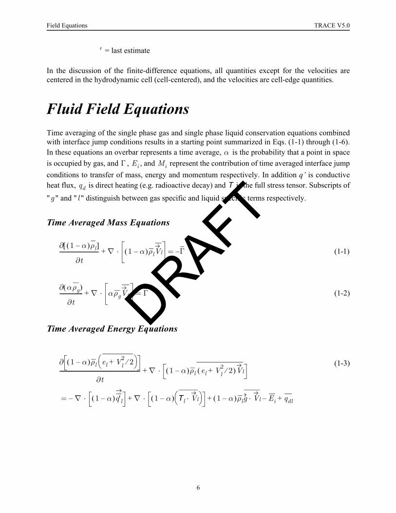
" " and " " distinguish between gas specific and liquid specific terms respectively.
Time Averaged Mass Equations
(1-1)
(1-2)
Time Averaged Energy Equations
(1-3)
′
αΓ Ei Mi
qd T
g l
1 α–( )ρl[ ]∂
t∂------------------------------ 1 α–( )ρlVl∇ · + Γ–=
αρg( )∂
t∂------------------ αρgVg∇ · + Γ=
1 α–( )ρl el V+ l2 2⁄⎝ ⎠
⎛ ⎞∂
t∂-------------------------------------------------------------- 1 α–( )ρl el V+ l
2 2⁄( )Vl∇ · +
1 α–( )q'l∇ · – 1 α–( ) Tl Vl·⎝ ⎠⎛ ⎞ 1 α–( )ρlg Vl· Ei– qdl+ +∇ · +=
DRAFT
6

TRACE V5.0 Field Equations
Field E
quations
(1-4)Time Averaged Momentum Equations
(1-5)
(1-6)
The equations are consistent with Reynolds averaging and splitting the velocities into mean andfluctuating contributions will yield expressions familiar to those who work with turbulence.However, contributions from the Reynolds stress, as well as most of the terms on the right handside of the energy and momentum equations will be modeled with engineering correlations, so thefollowing forms of the energy and momentum equations do not include full notation from classicturbulence formulation. In the energy equation the term q’ is redefined to include energy flux dueto turbulent diffusion. Energy carried with mass transfer at the interface is represented by theproducts of mass transfer rate and appropriate stagnation enthalpy at the interface (Γh’v and Γh’l).Work done on the fluid is split into that due to the pressure terms in the stress tensor, and a termsimply labeled "W", containing work done by shear stress and by interfacial force terms.
Revised Time Average Energy Equations
(1-7)
αρg eg V+ g2 2⁄⎝ ⎠
⎛ ⎞∂
t∂-------------------------------------------------- αρg eg V+ g
2 2⁄( )Vg∇ · +
αq'g∇ · – α Tg Vg·⎝ ⎠⎛ ⎞ αρgg Vg· Ei qdg+ + +∇ · +=
1 α–( )ρlVl∂
t∂------------------------------------- 1 α–( )ρlVlVl∇ · + 1 α–( )Tl[ ] 1 α–( )ρl g Mi–+∇ · =
αρgVg∂
t∂------------------------- αρgVgVg∇ · + αTg[ ] αρg g Mi+ +∇ · =
1 α–( )ρl el V+ l2 2⁄⎝ ⎠
⎛ ⎞∂
t∂--------------------------------------------------------------- 1 α–( )ρl el
Pρl---- V+ + l
22⁄⎝ ⎠
⎛ ⎞ Vl⎝ ⎠⎛ ⎞∇ · +
1 α–( )q'l 1 α–( )ρlg Vl Γ– h'l Wl qdl+ +·+∇ · –=
DRAFT
7

Field Equations TRACE V5.0
(1-8)
In the momentum equations pressure is also isolated from the stress tensor, and for purposes ofthis derivation the viscous shear stress terms are combined with the Reynolds stress into a singletensor .
Revised Time Average Momentum Equations
(1-9)
(1-10)
At this point it is possible to move on to the finite volume conservation equations. However, thenext round of approximations made in the TRACE flow model can also be illustrated byconsidering a volume averaged form of the above field equations. First the overbar is dropped andall variables are treated as time averages. Next the overbar is returned to the notation as a volumeaverage of terms in the conservation equations.
Volume Averaged Mass Equations
(1-11)
(1-12)
αρg eg V+ g2 2⁄⎝ ⎠
⎛ ⎞∂
t∂------------------------------------------------- αρg eg
Pρg----- V+ + g
22⁄⎝ ⎠
⎛ ⎞ Vg⎝ ⎠⎛ ⎞∇ · +
αq'g∇ · – αρg g Vg· Γh'v Wg qdg+ + ++=
R
1 α–( )ρlVl∂
t∂------------------------------------- 1 α–( )ρlVlVl∇ · + 1 α–( )Rl[ ] 1 α–( )ρl g Mi–+∇ · =
αρgVg∂
t∂------------------------- αρgVgVg∇ · + αRg[ ] αρg g Mi+ +∇ · =
1 α–( )ρl[ ]∂
t∂------------------------------ 1 α–( )ρlVl[ ]∇ · + Γ–=
αρg( )∂
t∂------------------- αρgVg∇ · + Γ=
DRAFT
8

TRACE V5.0 Field Equations
Field E
quations
Volume Averaged Energy Equations
(1-13)
(1-14)
Volume Averaged Momentum Equations
(1-15)
(1-16)
Now a series of approximations are made.
1) The volume average of a product is assumed to be equal to the product of volume averages. This is reasonable if the averaging volume is small enough, but eventually when applied within the finite volume context to reactor systems, the averaging vol-ume will span flow channels. In this case, the approximation is good for most turbu-lent flows due to the flat profile across most of the flow cross-section. However, for laminar single phase flow in a circular channel cross-section, when the average of the product of two parabolic profiles is replaced by the product of the average velocities, momentum flux terms will be low by 25%. Flows with rising droplets and falling wall film or certain vertical slug flows will also present problems.
1 α–( )ρl el V+ l2 2⁄( )∂
t∂--------------------------------------------------------------- 1 α–( )ρl el
Pρl
---- V+ + l
22⁄⎝ ⎠
⎛ ⎞ Vl∇ · +
1 α–( )q'l[ ]∇ · – 1 α–( )ρl g Vl Γ– h'i Wl+· qdl+ +=
αρg eg V+ g2 2⁄( )∂
t∂------------------------------------------------- αρg eg
Pρg----- V+ + g
22⁄⎝ ⎠
⎛ ⎞ Vg⎝ ⎠⎛ ⎞∇ · +
αq'g[ ]∇ · – αρgg Vg· Γh'v Wg+ qdg+ ++=
1 α–( )ρlVl[ ]∂
t∂------------------------------------- 1 α–( )ρlVlVl∇ · + 1 α–( )Rl[ ]∇ · 1 α–( )ρlg Mi–+=
αρgVg[ ]∂
t∂------------------------- αρgVgVg∇ · + αRg[ ]∇ · αρgg Mi+ +=
DRAFT
9
Field Equations TRACE V5.0
2) Only contributions from wall heat fluxes and heat fluxes at phase interfaces within the averaging volume are normally included in the volume average of the divergence of heat flux. An option exists to include the conduction heat flux within the fluid (perhaps useful for liquid metal flow), but no provision has been made for turbulent heat flux between averaging volumes. In effect, heat flux is a subgrid model. This approxima-tion prevents accurate calculations of such phenomena as collapse of a steam bubble blocking natural circulation through a B&W candy-cane, or of the details of steam condensation at the water surface in an AP1000 core makeup tank. From a practical standpoint, lack of the volume to volume heat diffusion terms will not make a major difference in a simulation. For any normal spatial discretization the numerical diffu-sion (see (Ref. 1-7)) will significantly exceed the physical thermal diffusion.
3) Only contributions from the stress tensor due to shear at metal surfaces or phase inter-faces within the averaging volume are considered. No contributions due to shear between flows in adjacent averaging volumes is included. Again from a practical standpoint, numerical diffusion terms exceed any physical terms dropped by this approximation. However, code users need to understand that field equations with this approximation are not capable of modeling circulation patterns within a large open region regardless of the choice of mesh size.
4) Only those portions of the work terms and that contribute to change in bulk kinetic energy of motion are retained. Viscous heating is ignored, except as a special model within pump components, accounting for heating of the fluid by a pump rotor. through the direct heating source term .
As a result of the first approximation, overbars are eliminated from the following equations, and acombination of time and volume average is implied for all state variables. At this point a switch ismade in the definition of α from a probability that a point is space is gas, to the fraction of theaveraging volume occupied by gas (void fraction). Heat transferred from the interface to gas andto liquid (W/m3) is represented by the terms and respectively. Similar expressions ( ,
) are used for heat transferred from surfaces of structures to the fluid. Expressions for all ofthese will come from correlations developed from steady state data, and they replace the heattransport terms in Equations (1-13) and (1-14) as shown in the following expressions
(1-17)
(1-18)
Under the third approximation the right hand sides of the momentum equations are changed to asimpler form:
Wl Wg
qdl
qig qil qwg
qwl
1 α–( )q'l[ ]∇ · qil qwl+⇒–
αq'g[ ]∇ · qig qwg+⇒–
DRAFT
10
TRACE V5.0 Field Equations
Field E
quations
(1-19)(1-20)
where is the force per unit volume due to shear at the phase interface, is the wall shear force
per unit volume acting on the liquid, is the wall shear force per unit volume acting on the gas,
and is the flow velocity at the phase interface.
Given the above notation for force terms, and the fourth assumption, the energy equations can bewritten in the form:
(1-21)
(1-22)
Under the notation used in Equations (1-19) through (1-22), the mass equations for the two fluidmodel, become:
(1-23)
1 α–( )ρlVl[ ]∂
t∂------------------------------------- 1 α–( )ρlVlVl∇ · 1 α–( ) P∇+ + fi fwl 1 α–( )ρlg ΓVi–+ +=
αρgVg[ ]∂
t∂------------------------- αρgVgVg∇ · α P∇+ + f– i fwg αρgg ΓVi+ + +=
fi fwl
fwg
Vi
1 α–( )ρl el V+ l2 2⁄( )∂
t∂------------------------------------------------------------- 1 α–( )ρl el
Pρl---- Vl
2 2⁄+ +⎝ ⎠⎛ ⎞ Vl∇ · +
qil qwl qdl 1 α–( )+ + ρl g Vl Γ– h'l fi fwl+( ) Vl·+·+=
αρg eg V+ g2 2⁄( )∂
t∂------------------------------------------------- αρg eg
Pρg----- Vg
2 2⁄+ +⎝ ⎠⎛ ⎞ Vg∇ · +
qig qwg qdg αρgg Vg· Γh'v fi– fwg+( ) Vg·+ + + + +=
1 α–( )ρl[ ]∂
t∂------------------------------ 1 α–( )ρlVl[ ]∇ · + Γ–=
DRAFT
11

Field Equations TRACE V5.0
(1-24)
Closure is obtained for these equations using normal thermodynamic relations and correlationsfor phase change, heat source and force terms. These equations do not directly require the quasi-steady assumption for the closure terms as long as the correct closure relations for the giventransient exist. A real difficulty arises because, depending on how the closure relations weredeveloped, a different set of closure relations may be required for each transient, and each setmust comply with the assumptions associated with the definition of the time- and volume-averaging used in the field equations. If a steady- or quasi-steady-state database or a relationshipderived from such a database is used to represent a closure relation, the code necessarily appliesthe quasi-steady assumption, as detailed in Appendix A. This latter case applies for the closurerelations within TRACE.
The phase-change rate required by the equation set is evaluated from a simple thermal-energy-jump relation, often called a heat conduction limited model.
(1-25)
where the interfacial heat transfer per unit volume on the gas and liquid sides are
(1-26)
and
. (1-27)
Here is the interfacial area per unit volume, and are HTCs at the liquid/gas interface,
and is the saturation temperature corresponding to the partial steam pressure ( ). Chapter
5 discusses the closure relationships used to define , , and . The quantities and arethe appropriate enthalpies of the vapor and liquid, respectively. These enthalpies are the bulk fluidenthalpy for the phase moving to the interface and the saturation enthalpy for the product of thephase change. This choice of enthalpies was inherited from both the RELAP and TRAC codeseries. Use of bulk enthalpy for the phase moving to the interface was necessary to preventunphysical thermal runaways.
One example of such runaway behavior can occur when subcooled liquid is driving thecondensation of a superheated vapor and the interfacial heat transfer on the gas side is very low.In this situation the bulk gas temperature increases if steam is removed at the interface at thesaturation temperature, but no significant interfacial heat transfer (diffusion) from bulk gas to
αρg( )∂
t∂------------------ αρgVg[ ]∇ · + Γ=
Γqig qil+( )–hv' hl'–( )
--------------------------=
qigPvP------higai Tsv Tv–( )=
qil hilai Tsv Tl–( )=
ai hig hil
Tsv Pv
ai hig hil hv' hl'
DRAFT
12

TRACE V5.0 Field Equations
Field E
quations
interface is present to provide a balancing cooling effect for the bulk gas. Removal of steam at atemperature less than the bulk temperature, leaves the remaining gas hotter. The root of thisproblem is in the use of the heat conduction limited model. It is meant for a diffusion dominatedprocess and the heat transfer coefficients selected to represent the boundary conditions at theinterface assume diffusion dominates the energy transfer. In fact when the full advection/diffusionproblem is considered the diffusive heat flux at the boundary is strongly enhanced as theadvection becomes important (see, for example, the temperature profiles in the advection/diffusion example presented by Roach (Ref. 1-8)). In this limit of negligible interfacial heattransfer on the gas side, use of the bulk gas temperature to evaluate the steam enthalpy in Eqs.(1-22) and (1-25) is rigorously correct. In any case, except for very unusual circumstances,temperatures are close enough to saturation that use of a bulk enthalpy rather than a saturationenthalpy in Eqs. (1-22) and (1-25) will make much less difference in results than the inherentrange of uncertainty associated with interfacial heat transfer equations.
Using Newton’s law of cooling extended to a thermal nonequilibrium situation, the wall heat-transfer terms assume the form
(1-28)
and
(1-29)
where is the heated surface area per volume of fluid (only meaningful in a volume averaged or
finite volume context). The heat transfer coefficients and include the informationregarding the portion of the wall having gas and liquid contact. Chapter 6 discusses the closurerelationships used to define and .
Force terms , , and are cast in the following forms, relying on correlations for friction
coefficients , . and .
(1-30)
(1-31)
(1-32)
By representing interfacial force with Eq. (1-30), two contributions to interfacial force have beenneglected. Terms proportional to acceleration (virtual mass terms) have been ignored because ofno evidence of significance in reactor safety problems, combined with significant increase in
qwg hwgaw Tw Tg–( ) q 'wgaw= =
qwl hwlaw Tw Tl–( ) q 'wl aw= =
aw
hwg hwl
hwg hwl
fi fwg fwl
Ci Cwg Cwl
fi Ci Vg Vl–( ) Vg Vl–=
fwg C– wgVg Vg=
fl C– wlVl Vl=
DRAFT
13
Field Equations TRACE V5.0
complexity of the solution procedure when they are present with semi-implicit or SETS solutionprocedures. Virtual mass terms will be reconsidered if higher order numerical methods areintroduced into a future version of TRACE and a well-posed set of PDEs becomes important. Liftforces perpendicular to the flow direction have also been dropped. However, some representationof this term will be necessary in future TRACE versions containing the ability to do sub-channelanalysis in a reactor core.
Rearrangement of Equations for Numerical Solution
TRACE does not solve the field equations in the form presented above. To cut complexity andcomputer time of the numerical solution, the fully conservative forms of the energy andmomentum equations are rearranged to provide internal energy and motion equations. The stepsto the next form of the field equations are rigorous mathematically, and involve no formalapproximations. However, in finite volume form, the internal energy equations have problemswith very large changes in pressure between two cells that are not present when the fullyconservative forms of the energy equations are implemented directly into a finite volumeapproach. In such cases the prediction of temperature change between two volumes deterioratessignificantly when the pressure change between the volumes is very large. This problem wasinherited from RELAP and TRAC, and from a practical standpoint has only been apparent whenthe code has been used to model both the reactor primary and the containment during a LOCA.Fortunately, one portion of the TRACE development effort was a task to provide direct time stepby time step linkage between parallel executions of TRACE and CONTAIN. CONTAIN wasdeveloped for the USNRC at Sandia National Laboratory to simulate a reactor containment’stransient behavior during a LOCA. In a coupled calculation TRACE only simulates the reactorcoolant system (vessel, primary loops, and steam generator secondary system) while CONTAINsimulates the containment side of the problem. Development of the linkage between TRACE andCONTAIN included adjustments to the energy flux terms between the codes to preserve thecorrect temperature change in fluid as it moves from a high pressure volume in TRACE to a lowpressure volume in CONTAIN.
Use of motion equations, rather than fully conservative momentum equations, generally worksvery well. However, exaggerated momentum transfer can occur in TRACE V5.0 (or earlier) whena steam/droplet mixture flows down towards the surface of a liquid pool (often in a downcomerduring reflood). When practical, the solution to this problem is to engage the TRACE interfacetracking model.
An internal energy conservation equation (gas or liquid) is obtained by taking the dot product ofthe corresponding momentum equation with its velocity and subtracting the results from the fullyconservative energy equation. For gas the result is:
(1-33)αρgeg( )∂
t∂----------------------- αρgegVg( )∇ · + P
t∂∂α P αVg( )∇ · –– qwg qdg qig Γhv'+ + + +=
DRAFT
14
TRACE V5.0 Field Equations
Field E
quations
A similar operation is performed on the liquid energy equation, but rather than using it in thatform, the result is added to the gas energy equation to produce a mixture energy conservationequation.
(1-34)
When included in the finite volume equation solution, the mixture energy equation makes it easierto deal with transitions from two-phase to single-phase flow during a step in the time integration.To fully achieve this advantage during a transition, a similar pair of gas and mixture massequations must be used in the actual solution.
(1-35)
(1-36)
Motion equations are obtained by the standard means of multiplying the mass conservationequation for a phase (Eq. (1-23) or Eq. (1-24)) by that phase’s velocity, subtracting it from thecorresponding momentum conservation equation (Eq. (1-19) or Eq. (1-20)), and dividing theresult by the appropriate macroscopic density.
(1-37)
(1-38)
Eq. (1-37) and Eq. (1-38) are generally referred to as the nonconservative form of the momentumequations, because it is not possible to write a finite volume method that guarantees somenumerical integral of momentum over a system does not change from one time step to the next in
1 α–( )ρlel αρgeg+∂
t∂--------------------------------------------------------- 1 α–( )ρlelVl αρgegVg+∇ · +
P 1 α–( )Vl αVg+∇ · – qwl qwg qdl qdg+ + + +=
αρg( )∂
t∂------------------ αρgVg[ ]∇ · + Γ=
1 α–( )ρl αρg+∂
t∂----------------------------------------------- 1 α–( )ρlVl αρgVg+∇ · + 0=
Vl∂
t∂--------- Vl Vl∇·+ 1
ρl---- P∇–
fi Γ Vi Vl–( )– fwl+
1 α–( )ρl------------------------------------------------------ g+ +=
Vg∂
t∂---------- Vg Vg∇·+ 1
ρg----- P∇–
fwg fi– Γ Vg Vi–( )–
αρg------------------------------------------------------ g+ +=
DRAFT
15
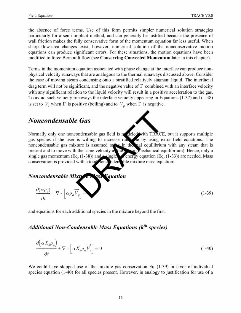
Field Equations TRACE V5.0
the absence of force terms. Use of this form permits simpler numerical solution strategiesparticularly for a semi-implicit method, and can generally be justified because the presence ofwall friction makes the fully conservative form of the momentum equation far less useful. Whensharp flow-area changes exist, however, numerical solution of the nonconservative motionequations can produce significant errors. For these situations, the motion equations have beenmodified to force Bernoulli flow (see Conserving Convected Momentum later in this chapter).
Terms in the momentum equation associated with phase change at the interface can produce non-physical velocity runaways that are analogous to the thermal runaways discussed above. Considerthe case of moving steam condensing onto a stratified relatively stagnant liquid. The interfacialdrag term will not be significant, and the negative value of combined with an interface velocitywith any significant relation to the liquid velocity will result in a positive acceleration to the gas.To avoid such velocity runaways the interface velocity appearing in Equations (1-37) and (1-38)is set to when is positive (boiling) and to when is negative.
Noncondensable Gas
Normally only one noncondensable gas field is modeled with TRACE, but it supports multiplegas species if the user is willing to increase run time by using extra field equations. Thenoncondensable gas mixture is assumed to be in thermal equilibrium with any steam that ispresent and to move with the same velocity as the steam (mechanical equilibrium). Hence, only asingle gas momentum (Eq. (1-38)) and a single gas energy equation (Eq. (1-33)) are needed. Massconservation is provided with a total noncondensable mixture mass equation:
Noncondensable Mixture Mass Equation
, (1-39)
and equations for each additional species in the mixture beyond the first.
Additional Non-Condensable Mass Equations (kth species)
(1-40)
We could have skipped use of the mixture gas conservation Eq. (1-39) in favor of individualspecies equation (1-40) for all species present. However, in analogy to justification for use of a
Γ
Vl Γ Vg Γ
αρa( )∂
t∂------------------ αρaVg∇ · + 0=
αXkρa⎝ ⎠⎛ ⎞∂
t∂-------------------------- αXkρaVg∇ · + 0=
DRAFT
16

TRACE V5.0 Field Equations
Field E
quations
full mixture mass equation (1-36), inclusion of the full mixture mass equation aids in enforcementof mass conservation when individual gas species disappear from a computational volume.
For pure non-condensable gases, air, and mixtures of these gases, an ideal gas equation of state isnormally assumed. The only exception occurs when helium is the only noncondensable gaspresent in a flow simulation. In that case, you are permitted to select a non-ideal helium equation(see Chapter 11). In terms of the ideal gas model, the mixture density is obtained from:
(1-41)
With this field present, the total gas density and energy are sums of the vapor and thenoncondensable components,
(1-42)
and
(1-43)
where specific internal energy of the noncondensable mixture is the sum of mass weightedcontributions from all noncondensable gas species.
(1-44)
We assume Dalton’s law applies; therefore,
. (1-45)
TRACE, by default, applies the thermodynamic properties for air to a single noncondensable gas.The code user may, however, select hydrogen, helium, nitrogen, argon, krypton, or xenon as thesingle gas, or use any of these in a mixture.
Liquid Solute
TRACE includes an optional mass-continuity equation for a solute (default is orthoboric acid)moving with the liquid field.
ρaP
RmixT----------------=
ρg ρv ρa+=
egρg evρv eaρa+=
ea XNC 1,
eNC 1,
XNC 2,
eNC 2,
…+ +=
P Pv Pa+= DRAFT
17

Field Equations TRACE V5.0
Liquid-Solute Concentration Equation
(1-46)
where m is the solute concentration (mass of solute/unit mass of liquid water) in the liquid phase.
The solute does not affect the hydrodynamics directly. However, the amount of the dissolved andthe plated-out orthoboric acid in a reactor core may affect the hydrodynamics indirectly throughneutronic-reactivity feedback corresponding to user-specified input values obtained from a boron-mass reactivity-coefficient table (see Chapter 9, Reactivity Feedback). If the solute concentrationexceeds the orthoboric-acid solubility at the liquid temperature in a specific hydrodynamic cell,TRACE assumes that the excess solute in that cell plates out. Plating on structures can occur if thecell liquid boils and thus increases the concentration beyond the solubility limit. TRACE alsoassumes that any plated-out solute instantaneously redissolves to the maximum allowableconcentration if more liquid enters the cell. Because the solute does not affect the hydrodynamicsdirectly, the solute variable may also be used as a tag to track the movement of liquid from aspecific source through the system.
Application Specific Usage of these EquationsTRACE utilizes the time and volume averaged equations presented in the previous section in twocontexts. The first is in a 1-D form in which fluid behavior in the other two dimensions is hiddenby an average of the flow over the cross-section of the flow channel. As will be seen below, thisprocedure permits modeling of flow channels with variable cross-sectional area, but loses theability to capture the effects of flow structures (e.g. recirculation zones) associated with changesin cross-sectional area. The second context is 3-D modeling, where a porous media approach isfollowed in the actual implementation. When the field equations are averaged over a 3-D region,provisions are made for metal structures filling portions of the geometric volumes and boundingflow areas, reducing the actual space available for flow. Changes of available flow area withinthis context, combined with sizes of the averaging volumes will also mask details of flowpatterns. In both cases empirical modeling is required to capture the average effects of flows notresolved. The primary contribution to this modeling seen by the user is the need to specifyempirical loss coefficients for the momentum equations.
1-D Equations
The use of the term "one-dimensional" in association with the equations used by TRACE tomodel piping in reactors or experiments can be an immediate source of confusion. The tendencyis to think in terms of three-dimensional Cartesian geometry, and a pipe running straight in asingle direction. However, piping runs in these systems have a number of bends, and a true one-
1 α–( )mρl[ ]∂
t∂------------------------------------ 1 α–( )mρlVl∇ · + Sm=
DRAFT
18
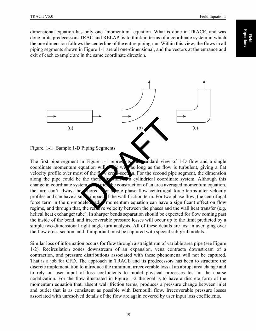
TRACE V5.0 Field Equations
Field E
quations
dimensional equation has only one "momentum" equation. What is done in TRACE, and wasdone in its predecessors TRAC and RELAP, is to think in terms of a coordinate system in whichthe one dimension follows the centerline of the entire piping run. Within this view, the flows in allpiping segments shown in Figure 1-1 are all one-dimensional, and the vectors at the entrance andexit of each example are in the same coordinate direction.
The first pipe segment in Figure 1-1 represents the standard view of 1-D flow and a singlecoordinate momentum equation will work well as long as the flow is turbulent, giving a flatvelocity profile over most of the flow cross-section. For the second pipe segment, the dimensionalong the pipe could be the theta direction in a cylindrical coordinate system. Although thischange in coordinate system simplifies the construction of an area averaged momentum equation,the turn can’t always be ignored. For single phase flow centrifugal force terms alter velocityprofiles and can have a small impact of the wall friction term. For two phase flow, the centrifugalforce term in the un-modeled radial momentum equation can have a significant effect on flowregime, and through that, the relative velocity between the phases and the wall heat transfer (e.g.helical heat exchanger tube). In sharper bends separation should be expected for flow coming pastthe inside of the bend, and irrecoverable pressure losses will occur up to the limit predicted by asimple two-dimensional right angle turn analysis. All of these details are lost in averaging overthe flow cross-section, and if important must be captured with special sub-grid models.
Similar loss of information occurs for flow through a straight run of variable area pipe (see Figure1-2). Recirculation zones downstream of an expansion, vena contracta downstream of acontraction, and pressure distributions associated with these phenomena will not be captured.That is a job for CFD. The approach in TRACE and its predecessors has been to structure thediscrete implementation to introduce the minimum irrecoverable loss at an abrupt area change andto rely on user input of loss coefficients to model physical processes lost in the coarsenodalization. For the flow illustrated in Figure 1-2 the goal is to have a discrete form of themomentum equation that, absent wall friction terms, produces a pressure change between inletand outlet that is as consistent as possible with Bernoulli flow. Irrecoverable pressure lossesassociated with unresolved details of the flow are again covered by user input loss coefficients.
Figure. 1-1. Sample 1-D Piping Segments
(a) (b) (c)
DRAFT
19

Field Equations TRACE V5.0
Pseudo 2-D Flow
One-dimensional modeling is complicated by the fact that pipes modeled by one dimensionalcross-section averaged equations can have connections through their walls from other pipes.Within reactor systems these connections are necessary to model Emergency Core CoolingSystems (ECCS) and jet pumps. Topologically, connections can range from a right angle "T",through angled connections to the wall, to injection pipes that are interior and parallel to a largerpipe at the point of injection (see Figure 1-3).
Derivations of the finite volume equations in the next section include provisions for such sidejunctions to a 1-D flow path. However, there are certain limitations within the current TRACE
Figure. 1-2. Abrupt Expansion and Contraction
Figure. 1-3. Tee connections
Side View
End View
(a) (b) (c)
DRAFT
20

TRACE V5.0 Field Equations
Field E
quations
implementation that should be noted now. For reactor system transients the injection flow patternsillustrated in Figure 1-3 are the situations where the momentum transport terms are the mostsignificant. In particular it is very important to transfer momentum correctly within a jet pumpmodel, and in situations where ECCS liquid is being injected into a steam flow through a reactorcoolant pipe. A rigorous formulation for momentum transfer terms has not been developed for thecase were flow is out through the side connection. When this happens in normal reactor scenarios,the split in mass flows between the main and side legs of the connection is driven by pressurerather than momentum terms. In addition TRACE currently expects the main channel to have aconstant cross-sectional area over the volume with the side flow connection. Abrupt area changesacross a volume containing a side junction can lead to distortions in momentum transfer terms. Ifthe impact of momentum transfer in such a location is not clearly understood to be minimal, userguidelines on nodalization at a side junction should be followed.
One aspect of outflow from a side junction has been given special treatment. When the mainchannel has stratified two-phase flow and a large enough pressure drop occurs through the sideconnection, the volume fraction of fluid pulled through the side junction is not equal to the meanvolume fraction in the main flow channel. TRACE uses a special offtake model, documented inChapter 10, to determine the void fraction of the fluid convected out of the side junction.
3-D Equations
The 3-D implementation of the field equations suffer from two primary limitations. The first hasalready been mentioned. There is no model for turbulent diffusion and shear between fluid cells,making TRACE unsuitable for modeling circulation patterns in large open regions. The second isrelated to the large computational volumes used in models of reactor vessels. Flow turns from thecold leg into the downcomer and normally from the downcomer to the lower plenum within asingle volume. This yields an irrecoverable pressure loss within the calculation that is the same ascan be obtained from a simple back of the envelop calculation for a sharp right angle turn. In factthe streamlines curve, and the pressure distribution is such that the actual pressure loss will be lessthan the right angle limit.
Basic Finite-Volume Approximations to the Flow EquationsTo avoid confusion a few words are necessary about notation used in this section. We use a fairlystandard notation to represent a volume integral. For example mass in a volume would be writtenas
(1-47)mass ρ VdV∫=
DRAFT
21

Field Equations TRACE V5.0
Unfortunately, an upper case "V" is also used when writing velocities. However, there will be nointegration over velocities in this documentation, so that the combination of a " " below anintegral sign and a " " should always be interpreted as a volume integral. To avoid confusionwhen integrals are not present in notation, we define
(1-48)
Integrals are further abreviated through use of overbar averaging notation. For example the meandensity in a volume is expressed as
(1-49)
The field equations introduced in the previous section have gone through a volume averagingprocess to generate the wall terms in the energy and momentum equations, and fit well with afinite volume solution approach. Consider the region in a flow channel illustrated in Figure 1-4. Inthis example the surface bounding the volume of fluid is divided into the channel wall area, and
three areas through which flow can occur. The integral form of the gas massconservation equation for this volume is:
(1-50)
or applying Gauss’ Theorem:
. (1-51)
Hence the time derivative of the total gas mass in the region can be written as:
(1-52)
where the positive sense of an area vector is directed out from the volume.
VdV
Vol VdV∫=
ρ
ρ VdV∫
⎝ ⎠⎜ ⎟⎛ ⎞
Vol-------------------------=
A1 A2 A3, ,( )
t∂∂ αρg Vd
V∫ αρgVg( )∇ · Vd
V∫+ Γ Vd
V∫=
t∂∂ αρg Vd
V∫ αρgVg dS·
S∫+ Γ Vd
V∫=
αρg( )∂
t∂------------------Vol αρgVg
⎝ ⎠⎜ ⎟⎛ ⎞
1A1· αρgVg
⎝ ⎠⎜ ⎟⎛ ⎞
2A2· αρgVg
⎝ ⎠⎜ ⎟⎛ ⎞
3A3·+ + + Γ Vol·=
DRAFT
22

TRACE V5.0 Field Equations
Field E
quations
Four approximations must be made to convert Eq. (1-52) to a useful discrete approximation to thegas mass conservation equation. First the volume average of vapor macroscopic density must berelated to the volume centered values. In TRACE, the simple first order assumption is made thatstate quantities are constant throughout a volume, so the volume average is taken to be equal tothe volume center value. The next approximation converts the partial derivative with respect totime to a simple algebraic expression, given as
, (1-53)
where:
1) a superscript " " denotes known values at the current level in time;
2) a superscript " " denotes a value at the next level in time that must be determined from solution of the equations; and
3) is the increment in time between levels and .
The third approximation is that for all expressions, the average of a product is equal to the productof individual average state variables. In this case, Eq. (1-52) becomes
. (1-54)
The fourth approximation relates values of state variables at volume edge flow faces to volumecentered quantities. In the case of Eq. (1-54), when void fraction and gas density are needed to
Figure. 1-4. Volume in a Flow Channel
A3
A1 A2
Aw
αρg( )∂
t∂------------------
αρgn 1+ αρg
n–
∆t-------------------------------------=
n
n 1+
∆t n n 1+
αρg∂
t∂-------------Vol αρgVg⎝ ⎠
⎛ ⎞1
A1· αρgVg⎝ ⎠⎛ ⎞
2A2· αρgVg⎝ ⎠
⎛ ⎞3
A3·+ + + Γ Vol·=
DRAFT
23

Field Equations TRACE V5.0
calculate a mass flux at a flow surface ( , , or ), the values are obtained from the nearestvolume center upstream (as determined by gas velocity) from the flow surface. This is a first orderupwind method. Momentum equations are evaluated at the edges of the volumes used for massand energy conservation, so no upwind approximation is needed to obtain the velocity used inmass flux terms. One important piece of information missing from Eq. (1-54) is the time level ofstate variables in the mass flux terms. Options for this choice within TRACE are discussed later inthis chapter.
Similar derivations can be followed to obtain discrete forms for other mass and energyconservation equations. For liquid mass or energy equations, the upwind cell center is determinedfrom the liquid velocity.
Generation of a discrete approximation to the momentum equation is more complex due to thefact that velocities and associated momentum equations are not evaluated at the same locations asthermodynamic state variables. Momentum equations and the primary associated velocities areevaluated at the surfaces separating the volumes used for conservation of mass and energy.
Figure 1-5 illustrates the edge (labeled ) between two adjacent mass/energy conservation
volumes ( and ). It illustrates the fact that a given computational volume can have a non-
uniform cross-sectional area, and that discontinuous changes in flow area can be modeled at thejunction between volumes. The center of a mass conservation volume is taken to be halfwaybetween the bounding flow surfaces along the center of the flow channel. Dotted lines throughthese center points represent surfaces that will bound a volume to be used in the derivation of thefinite volume form of the momentum equation. Since the fundamental evaluation of velocities isnot at these dotted surfaces through points and , a special averaging procedure is needed toobtain velocities at these surfaces for use in momentum transport terms. This needs to beconsistent with the upwind procedure discussed for the mass conservation equation. However,
Figure. 1-5. Two mass/energy conservation volumes
A1 A2 A3
j 1 2⁄+
j j 1+
j j+1j+½j-½
j j 1+
DRAFT
24

TRACE V5.0 Field Equations
Field E
quations
because rapid area changes are permitted from volume to volume, the upwind approach is appliedto volumetric flow rather than velocity and for the flow direction chosen in Figure 1-5 we get
and
.
A detailed derivation of the discrete momentum equation and an alternative derivation based uponkinetic energy are provided in Appendix B. However, key steps in the process are provided here.Figure 1-6 focuses on the momentum volume consisting of the right half of mass volume andleft half of mass volume . To cut the length of subscript notation, the surfaces at locations and in Figure 1-5 are now designated by subscripts 1 and 2 respectively and assigned areas
and . The central surface between the two mass volumes is given a subscript , and to
cover side junctions in the derivation, side flow through an area is permitted. Users need toknow that more than one such side junction may exist. Because of the upstream approximationsused for spatial averages, only those side junctions upstream from the center of the momentumcell can contribute to momentum fluxes. In the final implementation of the finite volumemomentum equation, this upstream requirement can result in a shift in association of a sidejunction from one momentum volume to its immediate neighbor as flow velocities switch sign.
Basic approximations used in generation of the final discrete equations are modified slightly.Thermodynamic state variables such as density, pressure, and volume fraction are still constant
Figure. 1-6. Momentum Volume
Vj 1+
Aj 1 2⁄+
Vj 1 2⁄+
Aj 1+-------------------------------------=
Vj
Aj 1 2⁄–
Vj 1 2⁄–
Aj------------------------------------=
jj 1+ j
j 1+A1 A2 c
A3
A3
A1 A2Ac
DRAFT
25

Field Equations TRACE V5.0
over mass conservation volumes, so within the momentum volume, density (for example) has oneuniform value upstream of the central flow area ( ), and a second uniform value downstream ofthe central area. However, it is the product of velocity and channel flow area (volumetric flow)that is treated as constant on either side of the central flow area.
As a simple example of generation of a discrete momentum equation, integrate the gasmomentum equation over the momentum volume associated with flow surface locatedbetween two mass/energy conservation volumes.
(1-55)
or
. (1-56)
Next integrate the mass conservation equations over the portions of the volume to the left andright of . Area vectors for areas 1 through 3 are chosen to have a positive sense out of themomentum volume. The area vector associated with an area splitting the momentum volume inthe middle has a sign convention that is positive towards end area 2.
(1-57)
and
(1-58)
Changing notation to use of the volume and area averages seen in the derivation of the finitevolume mass equation, the integrated momentum equation can be written as:
Ac
Ac
t∂∂ αρgVg( ) Vd
V∫ αρgVgVg( ) Sd·
S∫ α P∇ Vd
V∫+ + ΓVi fi fw αρg+ + +( ) Vd
V∫=
t∂∂ αρgVg( ) Vd
V∫ αρgVgVg( )k Ak·
k 1 3,=∑ α P∇ Vd
V∫+ + ΓVi fi fw αρg+ + +( ) Vd
V∫=
Ac
t∂∂ αρg( ) Vd
Vr
∫ αρgVg( )c Ac·– αρgVg( )2 A2·+ Γ VdVr
∫=
t∂∂ αρg( ) Vd
Vl
∫ αρgVg( )1 A1· αρgVg( )c+ Ac· αρgVg( )3 A3·+ + Γ VdVl
∫=
DRAFT
26

TRACE V5.0 Field Equations
Field E
quations
(1-59)
The mass equations for the left (subscript ) and right (subscript ) halves of the momentumvolume are:
(1-60)
and
(1-61)
Next rearrange these mass equations to get end fluxes along the primary direction of flow.
(1-62)
and
(1-63)
At this point we use the assumption that the volume average of the products is equal to theproduct of the volume averages. By this point all velocities are time averaged, and turbulenceeffects have been included in wall and interfacial force terms, so no further loss of turbulenceeffects is implied. As mentioned in the previous section, this assumption works well in mostcases, but some cases exist where this will introduce difficulties. To simplify notation beyond thispoint we will drop the bar over flow variables. Eq. (1-59) becomes:
(1-64)
t∂∂ αρgVg( )Vol
j 1 2⁄+αρgVgVg( )k Ak·
k 1 3,=∑
α P∇ Volj 1 2⁄+
+
+ ΓVi fi fw αρg+ + +⎝ ⎠⎛ ⎞ Vol
j 1 2⁄+=
l r
t∂∂ αρg( )Voll αρgVg( )1 A1· αρgVg( )c Ac· αρgVg( )3 A3·+ + + ΓlVoll=
t∂∂ αρg( )
rVolr αρgVg( )c Ac·– αρgVg( )2 A2·+ ΓrVolr=
αρgVg( )1 A1· ΓlVoll t∂∂ αρg( )
lVoll αρgVg( )c Ac·– αρgVg( )3 A3·––=
αρgVg( )2 A2· ΓrVolr t∂∂ αρg( )
rVolr αρgVg( )c Ac·+–=
t∂∂ αρgVg( )Vol
j 1 2⁄+αρgVgVg( )k Ak·
k 1 3,=∑
α P∇( )Volj 1 2⁄+
+
+ ΓVi fi fw αρg+ + +⎝ ⎠⎛ ⎞ Vol
j 1 2⁄+=
DRAFT
27

Field Equations TRACE V5.0
Flux terms in Eq. (1-64) are expanded by multiplying Eq. (1-62) by and Eq. (1-63) by
, giving us
(1-65)
. (1-66)
Eq. (1-65) and Eq. (1-66) provide expressions for the first two terms in the momentum fluxsummation from Eq. (1-64), giving:
(1-67)
or
(1-68)
Given that the only permitted location for area discontinuity is at the center of the momentumvolume, and that the final numerical method is restricted to first order accuracy, we can write:
Vg 1,
Vg 2,
αρgVgVg( )l Al· ΓlVg 1, Voll Vg 1, t∂∂ αρg( )
lVoll–
Vg 1, αρgVg( )c Ac·– Vg 1, αρgVg( )3 A3·–
=
αρgVgVg( )2 A2· ΓrVg 2, Volr Vg 2, t∂∂ αρg( )
rVolr– Vg 2, αρgVg( )c Ac·+=
αρgVgVg( )k Ak·k 1 3,=∑ Vg 2, αρgVg( )c Ac· Vg 1, αρgVg( )c Ac·–
Vg 3, Vg 1,–( ) αρgVg( )3 A3· ΓrVg 2, Volr ΓlVg 1, Voll
Vg 2, t∂∂ αρg( )
rVolr– Vg 1, t∂
∂ αρg( )lVoll–
+ + +
=
αρgVgVg( )k Ak·k 1 3,=∑ αρgVg( )c Ac Vg 2, Vg 1,–⎝ ⎠
⎛ ⎞·
Vg 3, Vg 1,–( ) αρgVg( )3 A3· ΓrVg 2, Volr ΓlVg 1, Voll
Vg 2, t∂∂ αρg( )
rVolr– Vg 1, t∂
∂ αρg( )lVoll–
+ + +
= DRAFT
28
TRACE V5.0 Field Equations
Field E
quations
(1-69)
and
(1-70)
Eqs. (1-69) and (1-70) can be substituted into Eq. (1-68), and the result substituted intoEq. (1-64), to give a simpler form of the finite volume momentum equation.
(1-71)
At this point, to obtain results useful for a computer solution, we need to employ the previouslymentioned assumptions about the spatial dependence of state variables within the volumes ofinterest. Here void fraction, densities, and pressure are taken as constant within the left portion ofthe momentum volume and a separate set of constant values over the right portion of themomentum volume. The basis functions for velocities are slightly modified to deal with thepossibility of discontinuous change in area at the center of the momentum volume. Rather thantaking the velocity to be constant, the product of area averaged velocity and area is taken asconstant.
Expressions for volume averages need to be reexamined under the first order assumptions toprovide useful forms for these terms. One additional quantity that will be useful in this contextwill be the distance "dx" along the primary flow path between bounding areas and . Threeof the averages in Eq. (1-71) are:
t∂∂ αρgVg( )Vol
j 1 2⁄+Vg 2, t∂
∂ αρg( )rVolr–
Vg 1, t∂∂ αρg( )
lVoll– αρg t∂
∂ Vg( )Volj 1 2⁄+
=
ΓVi Volj 1 2⁄+
ΓrVg 2, Volr– ΓlVg 1, Voll– Γ Vi Vg–( )Volj 1 2⁄+
=
αρg t∂∂ Vg( )Vol
j 1 2⁄+αρgVg( )c Ac Vg 2, Vg 1,–⎝ ⎠
⎛ ⎞·
Vg 3, Vg 1,–⎝ ⎠⎛ ⎞ αρgVg( )3 A3· α PVol
j 1 2⁄+∇
+
+ +
Γ Vi Vg–( ) fi fw αρg+ + + Volj 1 2⁄+
=
A1 A2
DRAFT
29

Field Equations TRACE V5.0
(1-72)
(1-73)
and
(1-74)
Evaluation of the total contribution of pressure forces is greatly simplified by the first orderassumption that state variables are constant over sub-regions of the integration volume. For thisparticular case with pressure and void constant to the left and right of , we divide the integral
of the pressure force term into integration over three sub-volumes. One is centered on with an
infinitesimal thickness perpendicular to . The other two sub-volumes cover the remainder of
the momentum volume to the left and right of . The integral over these two large volumes willbe zero because the pressure gradient is zero throughout both. However, the integral over thecentral volume is non-zero due to the discontinuity in pressure. The result is obtained through useof Heaviside step functions to represent the functional forms of pressure and void fraction.
(1-75)
αρg t∂∂ Vg( )Vol
j 1 2⁄+αρg t∂
∂ Vg( ) VdV∫ αρg t∂
∂ Vg( ) Ad xdA∫
xd∫
αρg t∂∂ Vg( ) Ad xd
A∫
xd∫ αρgdx( )l αρgdx( )r+
t∂∂ Vg c,( )Ac
αρg t∂∂ Vg c,( )Acdx
= =
= =
=
Γ Vi Vg–( )Volj 1 2⁄+
Γ Vi Vg–( ) VdV∫ Γ Vi Vg–( ) Ad xd
A∫
xd∫
Γ Vi Vg–( ) Ad xdA∫
xd∫ Γdx( )l Γdx( )r+[ ] Vi Vg–( )cAc
Γ Vi Vg–( )c Acdx
= =
= =
=
αρg gVolj 1 2⁄+
αρg g VdV∫ αρg( )lVoll gl αρg( )rVolr gr+ αρg g Vol
j 1 2⁄+= = =
Ac
Ac
Ac
Ac
α∇P VdV∫ Ac α∇P xd
δ–
δ
∫ Acαl αr+( )
2---------------------- Pr Pl–( )= =
DRAFT
30
TRACE V5.0 Field Equations
Field E
quations
For those accustomed to the derivation of loss coefficients for an abrupt expansion, thisapproximation will look wrong. In the classic abrupt expansion case, the pressure is assumedto also be appropriate in the right sub-volume over the wall area aligned with the center surface ofthe momentum volume. Unfortunately, the finite volume calculation must be able to deal with awide variety of channel shapes. Rather than doing subgrid calculations to obtain better values ofsurface pressure distributions, we have elected to account for the discrepancy by using losscoefficients. The approach taken in Eq. (1-75) produces the lowest irrecoverable pressure loss ofall possible assumptions about wall pressure distribution. It is up to the user to provide losscoefficients in the model’s input specification that result in the correct irrecoverable pressure loss.
The force terms for interfacial and wall shear have proportionality to velocity, so the volume
multiplying those terms ( ) can be converted to the product . Substituting all of
the approximations to the volume integrals into the last form of the momentum equation and
dividing everything by gives
(1-76)
The actual momentum equations in TRACE were derived from a finite difference approach, andratios with the product of volume fraction and density in numerator and denominator are set toone.
(1-77)
To this point the time and volume averaged momentum equation is still 3-D. Three steps arenecessary to make it useful for a 1-D model. First the equation is recast into a coordinate systemin which one dimension follows the flow channel. From the standpoint of this coordinate system,there are no bends in the piping. The piping’s centerline can be treated as the axis of the primarydimension. Second, take the dot product of Eq. (1-77) with a unit vector along the primarydimension to isolate the component of the velocity along the piping. Finally introduce a term toaccount for irrecoverable losses lost in the volume averaging and collapse to one dimension. This
P1
Volj 1 2⁄+
Ac dx·
αρgAcdx
t∂∂ Vg( )
αρgVg( )cαρg Acdx----------------------- Ac Vg 2, Vg 1,–⎝ ⎠
⎛ ⎞·Vg 3, Vg 1,–⎝ ⎠
⎛ ⎞
αρg Acdx------------------------------------ αρgVg( )3 A3·
α pr pl–( )
αρg dx------------------------ i
+ +
+ 1αρg--------- Γ Vi c, Vg c,–( ) f
i c,fw c,
αρg gVol
j 1 2⁄+
Acdx-----------------------+ + +=
t∂∂ Vg( )
Vg( )cAcdx------------- Ac Vg 2, Vg 1,–⎝ ⎠
⎛ ⎞·Vg 3, Vg 1,–⎝ ⎠
⎛ ⎞
αρg Acdx------------------------------------ αρgVg( )3 A3·
α pr pl–( )
αρg dx------------------------ i
+ +
+ 1αρg--------- Γ Vi c, Vg c,–( ) f
i c,fw c,
+ + g+=
DRAFT
31
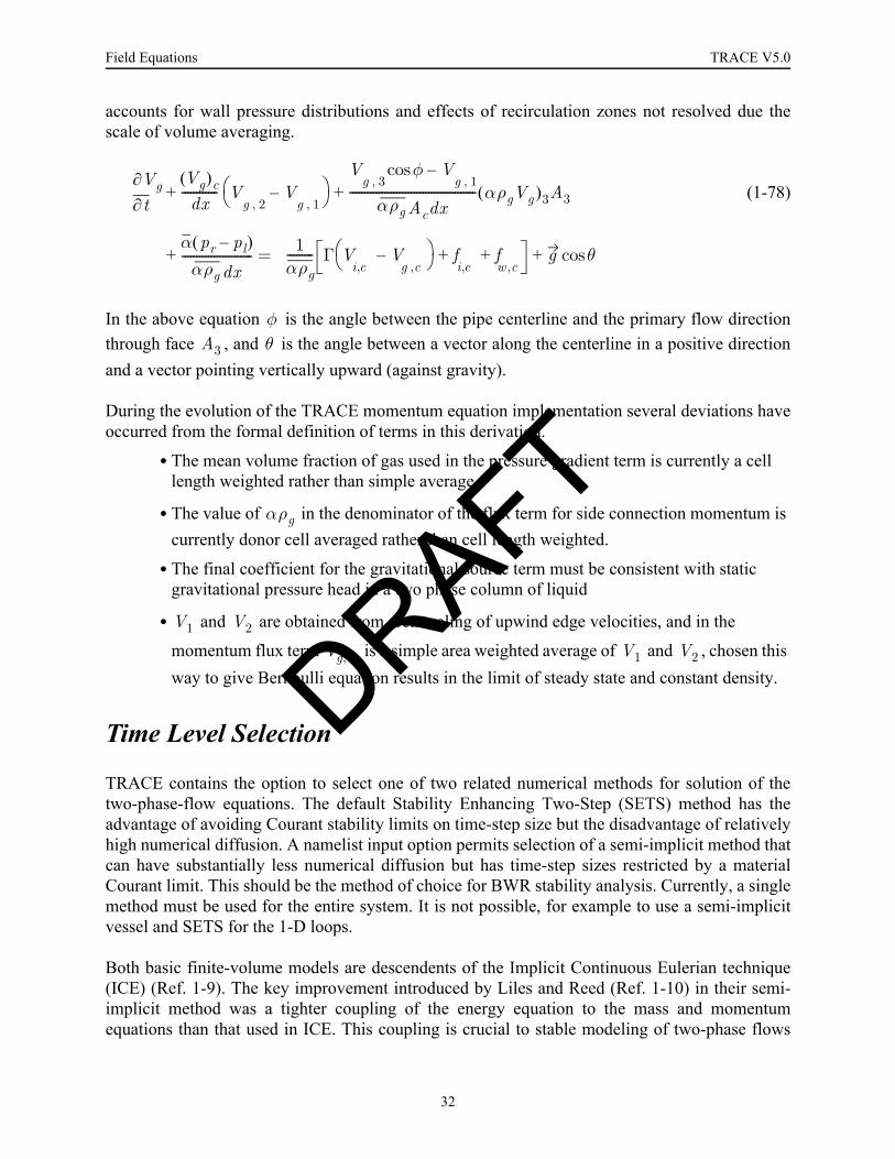
Field Equations TRACE V5.0
accounts for wall pressure distributions and effects of recirculation zones not resolved due thescale of volume averaging.
(1-78)
In the above equation is the angle between the pipe centerline and the primary flow directionthrough face , and is the angle between a vector along the centerline in a positive directionand a vector pointing vertically upward (against gravity).
During the evolution of the TRACE momentum equation implementation several deviations haveoccurred from the formal definition of terms in this derivation.
•The mean volume fraction of gas used in the pressure gradient term is currently a cell length weighted rather than simple average.
•The value of in the denominator of the flux term for side connection momentum is currently donor cell averaged rather than cell length weighted.
•The final coefficient for the gravitational source term must be consistent with static gravitational pressure head in a two phase column of liquid
• and are obtained from area scaling of upwind edge velocities, and in the
momentum flux term is a simple area weighted average of and , chosen this way to give Bernoulli equation results in the limit of steady state and constant density.
Time Level Selection
TRACE contains the option to select one of two related numerical methods for solution of thetwo-phase-flow equations. The default Stability Enhancing Two-Step (SETS) method has theadvantage of avoiding Courant stability limits on time-step size but the disadvantage of relativelyhigh numerical diffusion. A namelist input option permits selection of a semi-implicit method thatcan have substantially less numerical diffusion but has time-step sizes restricted by a materialCourant limit. This should be the method of choice for BWR stability analysis. Currently, a singlemethod must be used for the entire system. It is not possible, for example to use a semi-implicitvessel and SETS for the 1-D loops.
Both basic finite-volume models are descendents of the Implicit Continuous Eulerian technique(ICE) (Ref. 1-9). The key improvement introduced by Liles and Reed (Ref. 1-10) in their semi-implicit method was a tighter coupling of the energy equation to the mass and momentumequations than that used in ICE. This coupling is crucial to stable modeling of two-phase flows
t∂∂Vg Vg( )c
dx------------ V
g 2,V
g 1,–⎝ ⎠
⎛ ⎞V
g 3,φcos V
g 1,–
αρg Acdx------------------------------------------- αρgVg( )3A3
α pr pl–( )
αρg dx------------------------
+ +
+ 1αρg--------- Γ V
i c,V
g c,–⎝ ⎠
⎛ ⎞ fi c,
fw c,
+ + g θcos+=
φA3 θ
αρg
V1 V2
Vg c, V1 V2
DRAFT
32

TRACE V5.0 Field Equations
Field E
quations
with substantial boiling or condensation. The SETS method (Refs. 1-11 and 1-12) includes thesemi-implicit method at its core and increases stability with an additional evaluation of each fieldequation during each time step.
In the following subsections, the semi-implicit and SETS methods will be described at threelevels of detail. The basic aspects of each method are illustrated for simple 1D single-phase-flowequations as follows:
, (1-79)
, (1-80)
and
, (1-81)
where is a wall friction coefficient that may be a function of velocity and fluid properties and is a pipe wall temperature. More detail is then provided through explanation of special
adaptations to improve robust simulation of single- and/or two-phase flow. Finally, the full two-phase-flow equations are presented.
Fairly standard notation is used in presenting the finite-volume equations. A superscript “ ”indicates known values at the beginning of a step in the time integration (old-time value). Asuperscript “ ” labels a variable value at the end of the current time step (new-time value),which must be obtained as part of the solution of the equations. Subscripts provide information onspatial location as illustrated in Figure 1-5. Integer subscripts such as “ ” or “ ” label volume
center information (e.g., is the new-time pressure in volume “ ”). A half-integer subscript
indicates a value obtained at the surface separating two volumes (e.g., is the old-time
velocity at the surface separating volume “ ” from volume “ ”).
When values of cell-centered variables are needed at cell edges, an average of some form isrequired. The methods discussed here use values only from the volumes immediately adjacent tothe given edge, so the averages are always in the following form:
. (1-82)
ρ∂∂t------
x∂∂+ ρV( ) 0=
∂ ρe( )∂t
--------------x∂
∂+ ρeV( ) P∂V∂x--------– hw
Awvol-------- Tw T–( )+=
∂V∂t-------- V+ ∂V
∂x-------- 1
ρ---– ∂P∂x------- KV V–=
KTw
n
n 1+
j j 1+
Pjn 1+ j
Vj 1 2⁄+n
j j 1+
Y⟨ ⟩j 1 2⁄+
wj 1 2⁄+
= Yj 1 wj 1 2⁄+
–( )Yj 1++
DRAFT
33

Field Equations TRACE V5.0
For simple 1D flow, terms expressing mass and energy flow for the finite volume then havethe following form:
. (1-83)
The form is more complex for 1D flow with a spatially varying cross-sectional flow area. In thiscase the mass flux term is abbreviated as
, (1-84)
where is the flow area between cells and and is the volume of the jth cell.
The related derivative used in the finite-difference momentum flux involves the use of a morecomplicated averaging method. This is driven by a need to model Bernoulli flows whenappropriate and to conserve momentum properly when a side-junction flow is present. Details ofthis methodology are presented in Conserving Convected Momentum. To aid in understandingthe basic numerical methods, it is worth noting that with no area changes or side junctions, thenumerical form of the velocity gradient is
. (1-85)
For flows in 1D channels with variable cross-sectional area, the momentum-transfer term isabbreviated as .
Although the basics of the finite volume spatial discretization have already been covered, furtherdetails are provided in later sections of this document. 3D Finite-Difference Methods presents ageneralization of the methods to 3D geometry. Special treatment of transition to single-phase flowand conditions beyond the critical point is described in Modifications to the Basic Equation Set.The section Conserving Convected Momentum describes details of special treatment used formomentum-flux terms. The actual solution of these equations is described in Chapter 2.
jth
∂∂xj-------- YV( )
Y⟨ ⟩j 1 2⁄+
Vj 1 2⁄+
Y⟨ ⟩j 1 2⁄–
– Vj 1 2⁄–
x∆--------------------------------------------------------------------------------------------
wj 1 2⁄+
Yj 1 wj 1 2⁄+
–⎝ ⎠⎛ ⎞ Yj 1++ V
j 1 2⁄+w
j 1 2⁄–Yj 1– 1 w
j 1 2⁄––⎝ ⎠
⎛ ⎞ Yj+ Vj 1 2⁄–
–
x∆------------------------------------------------------------------------------------------------------------------------------------------------------------------------------------------------------------------
=
=
∇j YV( )·
wj 1 2⁄+
Yj 1 wj 1 2⁄+
–⎝ ⎠⎛ ⎞+ Yj 1+ A
j 1 2⁄+V
j 1 2⁄+⎝ ⎠⎛ ⎞ w
j 1 2⁄–Yj 1– 1 w
j 1 2⁄––⎝ ⎠
⎛ ⎞+ Yj Aj 1 2⁄–
Vj 1 2⁄–⎝ ⎠
⎛ ⎞–
volj--------------------------------------------------------------------------------------------------------------------------------------------------------------------------------------------------------------------------------------------------------------------
=
Aj 1 2⁄+
j j 1+ volj
∂V∂x--------
j 1 2⁄+
1 wj 1 2⁄+
–( )Vj 3 2⁄+
2wj 1 2⁄+
1–( )Vj 1 2⁄+
wj 1 2⁄+
– Vj 1 2⁄–
+
x∆--------------------------------------------------------------------------------------------------------------------------------------------------------=
Vj 1 2⁄+
∇j 1 2⁄+
V
DRAFT
34

TRACE V5.0 Field Equations
Field E
quations
Basics of the Semi-Implicit Method
When fluid flow is modeled with a fully explicit method, time-step sizes are restricted by theCourant limit as
, (1-86)
where is a characteristic mesh length, is the flow velocity, is the speed of sound, andparameter varies in value depending on the details of the method, but here can be taken to be1.0. This simple class of methods is appropriate when it is important to track the details ofpressure wave propagation (e.g., shock waves). However, in most reactor transients, this level ofdetail is not important. At most, continuity waves (moving liquid levels or froth fronts) must befollowed. Frequently the transient is simply an evolution between quasi-steady states.
Both the ICE and semi-implicit methods relax the explicit restrictions on time-step size byevaluating terms involved in pressure wave propagation at the new ( ) time level. For asimple form of the momentum equation, this requires new-time values in the pressure gradientterm as given by
. (1-87)
Similarly, relaxation of the restrictions on time-step size also requires that velocities involved influx of mass and energy be evaluated at the new-time level. The equations then become
(1-88)
and
. (1-89)
t k≤∆ x∆V c+----------------·
∆x V ck
n 1+
Vj 1 2⁄+n 1+ V
j 1 2⁄+n–⎝ ⎠
⎛ ⎞
t∆------------------------------------------------ V
j 1 2⁄+n ∂Vn
∂x-----------
j 1 2⁄+
1ρ⟨ ⟩
j 1 2⁄+n----------------------
Pj 1+n 1+ Pj
n 1+–( )x∆
--------------------------------------- Kj 1 2⁄+n V
j 1 2⁄+n 1+ V
j 1 2⁄+n+ 0=
+
+
ρjn 1+ ρj
n–( )∆t
------------------------------xj∂∂ ρnVn 1+( )+ 0=
ρjn 1+ ej
n 1+ ρjnej
n–( )∆t
-------------------------------------------------xj∂∂ ρnenVn 1+( ) Pj
n 1++ +Vj 1 2⁄+
n 1+Vj 1 2⁄–
n 1+–⎝ ⎠⎛ ⎞
x∆-----------------------------------------------
=heat sources (W/m3 )
DRAFT
35
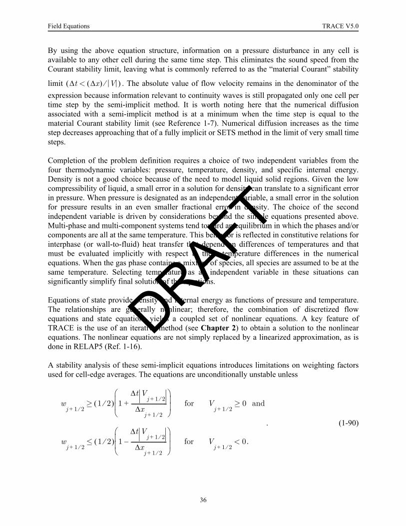
Field Equations TRACE V5.0
By using the above equation structure, information on a pressure disturbance in any cell isavailable to any other cell during the same time step. This eliminates the sound speed from theCourant stability limit, leaving what is commonly referred to as the “material Courant” stability
limit . The absolute value of flow velocity remains in the denominator of theexpression because information relevant to continuity waves is still propagated only one cell pertime step by the semi-implicit method. It is worth noting here that the numerical diffusionassociated with a semi-implicit method is at a minimum when the time step is equal to thematerial Courant stability limit (see Reference 1-7). Numerical diffusion increases as the timestep decreases approaching that of a fully implicit or SETS method in the limit of very small timesteps.
Completion of the problem definition requires a choice of two independent variables from thefour thermodynamic variables: pressure, temperature, density, and specific internal energy.Density is not a good choice because of the need to model liquid solid regions. Given the lowcompressibility of liquid, a small error in a solution for density can translate to a significant errorin pressure. When pressure is designated as an independent variable, a small error in the solutionfor pressure results in an even smaller fractional error in density. The choice of the secondindependent variable is driven by considerations beyond the simple equations presented above.Multi-phase and multi-component systems tend toward an equilibrium in which the phases and/orcomponents are all at the same temperature. This behavior is reflected in constitutive relations forinterphase (or wall-to-fluid) heat transfer that depend on differences of temperatures and thatmust be evaluated implicitly with respect to these temperature differences in the numericalequations. When the gas phase contains a mixture of species, all species are assumed to be at thesame temperature. Selecting temperature as an independent variable in these situations cansignificantly simplify final solution of the equations.
Equations of state provide density and internal energy as functions of pressure and temperature.The relationships are generally nonlinear; therefore, the combination of discretized flowequations and state equations yields a coupled set of nonlinear equations. A key feature ofTRACE is the use of an iterative method (see Chapter 2) to obtain a solution to the nonlinearequations. The nonlinear equations are not simply replaced by a linearized approximation, as isdone in RELAP5 (Ref. 1-16).
A stability analysis of these semi-implicit equations introduces limitations on weighting factorsused for cell-edge averages. The equations are unconditionally unstable unless
. (1-90)
t x∆( ) V⁄<∆( )
wj 1 2⁄+
1 2⁄( ) 1t V
j 1 2⁄+∆
xj 1 2⁄+
∆---------------------------+
⎝ ⎠⎜ ⎟⎜ ⎟⎛ ⎞
for Vj 1 2⁄+
0≥ and≥
wj 1 2⁄+
1 2⁄( ) 1t V
j 1 2⁄+∆
xj 1 2⁄+
∆---------------------------–
⎝ ⎠⎜ ⎟⎜ ⎟⎛ ⎞
for Vj 1 2⁄+
0. <≤
DRAFT
36
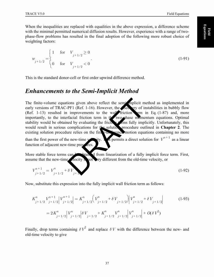
TRACE V5.0 Field Equations
Field E
quations
When the inequalities are replaced with equalities in the above expression, a difference schemewith the minimal permitted numerical diffusion results. However, experience with a range of two-phase-flow problems has resulted in the final adoption of the following more robust choice ofweighting factors:
. (1-91)
This is the standard donor-cell or first order upwind difference method.
Enhancements to the Semi-Implicit Method
The finite-volume equations given above reflect the semi-implicit method as implemented inearly versions of TRAC-PF1 (Ref. 1-16). However, the discovery of instabilities in bubbly flow(Ref. 1-13) resulted in improvements to the wall friction term in Eq. (1-87) and, moreimportantly, to the interfacial friction term in the two-phase momentum equations. Optimalstability would be obtained by evaluating the friction terms fully implicitly. Unfortunately, thiswould result in serious complications for the solution procedure outlined in Chapter 2. Theexisting solution procedure relies on the finite-difference motion equations containing no more
than the first power of the new-time velocity. This permits a direct solution for as a linearfunction of adjacent new-time pressures.
More stable force terms can be obtained from linearization of a fully implicit force term. First,assume that the new-time velocity is not very different from the old-time velocity, or
. (1-92)
Now, substitute this expression into the fully implicit wall friction term as follows:
(1-93)
Finally, drop terms containing and replace with the difference between the new- andold-time velocity to give
wj 1 2⁄+
1 for Vj 1 2⁄+
0≥
0 for Vj 1 2⁄+
0<⎩⎪⎨⎪⎧
=
Vn 1+
Vj 1 2⁄+n 1+ V
j 1 2⁄+n δV
j 1 2⁄++=
Kj 1 2⁄+n V
j 1 2⁄+n 1+ V
j 1 2⁄+n 1+ K
j 1 2⁄+n V
j 1 2⁄+n δV
j 1 2⁄++⎝ ⎠
⎛ ⎞ Vj 1 2⁄+n δV
j 1 2⁄++
2Kj 1 2⁄+n V
j 1 2⁄+n δV
j 1 2⁄+K
j 1 2⁄+n V
j 1 2⁄+n V
j 1 2⁄+n O δV2( )++
=
=
δV2 δV
DRAFT
37
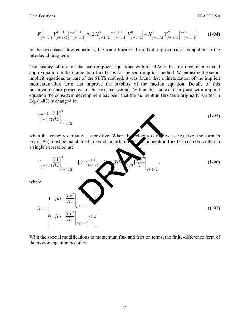
Field Equations TRACE V5.0
. (1-94)
In the two-phase-flow equations, the same linearized implicit approximation is applied to theinterfacial drag term.
The history of use of the semi-implicit equations within TRACE has resulted in a relatedapproximation in the momentum flux terms for the semi-implicit method. When using the semi-implicit equations as part of the SETS method, it was found that a linearization of the implicitmomentum-flux term can improve the stability of the motion equation. Details of thislinearization are presented in the next subsection. Within the context of a pure semi-implicitequation the consistent development has been that the momentum flux term originally written inEq. (1-87) is changed to:
(1-95)
when the velocity derivative is positive. When the velocity derivative is negative, the form inEq. (1-87) must be maintained to avoid an instability. The momentum flux term can be written ina single expression as:
, (1-96)
where
. (1-97)
With the special modifications to momentum flux and friction terms, the finite-difference form ofthe motion equation becomes
Kj 1 2⁄+n V
j 1 2⁄+n 1+ V
j 1 2⁄+n 1+ 2≈ K
j 1 2⁄+n V
j 1 2⁄+n 1+ V
j 1 2⁄+n K
j 1 2⁄+n V
j 1 2⁄+n V
j 1 2⁄+n–
Vj 1 2⁄+n 1+ ∂V
∂x--------
j 1 2⁄+
n
Vj 1 2⁄+
∂V∂x--------
j 1 2⁄+
nβV
j 1 2⁄+n 1+ 1 β–( )V
j 1 2⁄+n+[ ]∂Vn
∂x-----------
j 1 2⁄+
=
β
1 for ∂Vn
∂x-----------
j 1 2⁄+
0≥
0 for ∂Vn
∂x-----------
j 1 2⁄+
0<=
DRAFT
38

TRACE V5.0 Field Equations
Field E
quations
. (1-98)Semi-Implicit Method Adapted to Two-Phase Flow
Extension of the numerical method to the two-phase, two-fluid model is relativelystraightforward. Special modifications to the method are necessary to treat changes from two-phase to single-phase flow and are described below. Source terms are present to model phasechange and heat transfer. These are generally implicit in any driving temperature difference andexplicit in any coefficient. The importance of gravitationally driven liquid flow requires anaccurate model of gravitational force along the direction of motion. This uses an input angle ( )between a vector from the center of cell to the center of cell and a vector directed againstgravity. In the application of the code, is more generally the inverse cosine (cos–1) of the changein elevation between cell centers divided by the flow length between cell centers.
To shorten notation in the following difference equations, some subscripts associated withlocation have been eliminated. For velocities not contained in spatial differences, the subscript
denoting spatial location is assumed to be . For cell-centered variables, the assumed
subscript is . The phrase “combined gas” refers to the mixture of noncondensable gas and steam,which is assumed to move with no interspecies diffusion.
Semi-Implicit Equations of Motion
Combined Gas
+
Vj 1 2⁄+n 1+ Vn
j 1 2⁄+–( )
∆t-------------------------------------------------- βV
j 1 2⁄+n 1+ 1 β–( )V
j 1 2⁄+n++ ∂Vn
∂x-----------⎝ ⎠
⎛ ⎞
j 1 2⁄+
1ρ⟨ ⟩
j 1 2⁄+n
----------------------Pj 1+
n 1+ Pjn 1+–( )
∆x--------------------------------------- 2K
j 1 2⁄+n V
j 1 2⁄+n 1+ Vn
j 1 2⁄+
Kj 1 2⁄+
nV
j 1 2⁄+n V
j 1 2⁄+n– 0=
+ +
θj j 1+
θ
j 1 2⁄+
j
Vgn 1+ Vg
n–( )t∆
-------------------------------- βgVgn 1+ 1 βg–( )Vg
n+[ ]∇j 1 2⁄+
Vgn+
Cin Vg
n Vln–
αρg⟨ ⟩j 1 2⁄+
n------------------------------- 2 Vgn 1+ Vl
n 1+–( ) Vgn Vl
n–( )–[ ]
DRAFT
39

Field Equations TRACE V5.0
+
+ . (1-99)
Liquid
+
+
+ . (1-100)
Semi-Implicit Mass Equations
Combined Gas
. (1-101)
Noncondensable Gas
. (1-102)
Additional Noncondensable Mass Equations (kth species)
(1-103)
1ρg⟨ ⟩
j 1 2⁄+n-------------------------
Pj 1+n 1+ Pj
n 1+–( )∆x
j 1 2⁄+
---------------------------------------Γ
j 1 2⁄++n
αρg⟨ ⟩j 1 2⁄+n----------------------------- Vg
n 1+ Vln 1+–( )+
Cwg
αρg⟨ ⟩j 1 2⁄+n
----------------------------- 2Vgn 1+ Vg
n–( ) Vgn g θcos+ 0=
Vln 1+ Vl
n–t∆
---------------------------- βlVln 1+ 1 βl–( )Vl
n+[ ]∇j 1 2⁄+
Vln+
Cin Vl
n Vgn–
1 α–( )ρl⟨ ⟩j 1 2⁄+n--------------------------------------- 2 Vl
n 1+ Vgn 1+–( ) Vl
n Vgn–( )–[ ]
1ρl⟨ ⟩
j 1 2⁄+n------------------------
Pj 1+n 1+ Pj
n 1+–( )∆x
j 1 2⁄+
---------------------------------------Γ
j 1 2⁄+-n
1 α–( )ρl⟨ ⟩j 1 2⁄+n------------------------------------------ Vl
n 1+ Vgn 1+–( )–
Cwl
1 α–( )ρl⟨ ⟩j 1 2⁄+n
--------------------------------------- 2Vln 1+ Vl
n–( ) Vln g θcos+ 0=
αjn 1+ ρgj
n 1+ αjnρgj
n–∆t
------------------------------------------------ ∇j αnρgnVg
n 1+[ ]·+ Γn 1+=
αjn 1+ ρaj
n 1+ αjnρaj
n–[ ]t∆
----------------------------------------------------- ∇j αnρanVg
n 1+[ ]·+ 0=
αXkρa[ ]jn 1+ αXkρa[ ]j
n–∆t
-------------------------------------------------------------- ∇j αXkρa( )nVgn 1+
[ ]·+ 0=
DRAFT
40

TRACE V5.0 Field Equations
Field E
quations
Liquid
. (1-104)
Semi-Implicit Energy Equations
Combined Gas
+
. (1-105)
Total Fluid (gas and liquid)
+
+
. (1-106)
The wall heat transfer to the gas and liquid, and , and the interfacial mass-transfer rate, ,also require further definition. Note the mixture of old- and new-time values in these terms. Thechoice of old-time heat-transfer coefficients was driven by the desire to simplify theimplementation of the method, but can result in bounded instabilities during calculations. Theseterms are given by
, (1-107)
, (1-108)
and
1 αjn 1+–( )ρlj
n 1+ 1 α– jn( )ρlj
n–[ ]t∆
----------------------------------------------------------------------------- ∇j 1 αn–( )ρlnVl
n 1+[ ]·+ Γn 1+–=
αjn 1+ ρgj
n 1+ egjn 1+ αj
n– ρgjn egj
n[ ]t∆
----------------------------------------------------------------------- ∇j αnρgneg
nVgn 1+
[ ]·+
Pn 1+ αn 1+ αn–( )t∆
------------------------------- ∇j αnVgn 1+
( )·+
qwgn 1+ qdg
n qign 1+ Γn 1+ hsg
n 1++ + +=
αjn 1+ ρgj
n 1+ egjn 1+ 1 αj
n 1+–( )+ ρljn 1+ elj
n 1+[ ] αjnρgj
n egjn 1 αj
n–( ) ρljnelj
n( )+–t∆
------------------------------------------------------------------------------------------------------------------------------------------------------------------------------
∇j αnρgneg
nVgn 1+ 1 αn–( )ρl
nelnVl
n 1++[ ]·
Pn 1+ ∇j 1 α–( )nVln 1+ αnVg
n 1++[ ]·
qwgn 1+ qwl
n 1+ qdln qdg
n+ + +=
qwg qwl Γ
qwln 1+ hwl
n aw Twn 1+ Tl
n 1+–( )=
qwgn 1+ hwg
n aw Twn 1+ Tg
n 1+–( )=
DRAFT
41
Field Equations TRACE V5.0
, (1-109)
where
(1-110)
and
. (1-111)
The interfacial heat transfer coefficients ( , ), wall heat transfer coefficients ( , ),
interfacial drag coefficient ( ) and wall friction coefficients ( , ) all are the result ofnonlinear functions associated obtained from correlations. Old time (explicit) evaluation of thesecoefficients can result in bounded instabilities.
Further definition is also needed for a special set of density averages used in the momentumequations. Cell-edge densities used in the denominator of Eq. (1-99) and Eq. (1-100) are definedto produce a good prediction of hydrostatic pressure heads. For example, the edge-average gasmacroscopic density is defined as
. (1-112)
A similar definition holds for the cell-edge liquid macroscopic density. The edge-averagemicroscopic densities are somewhat more complex. For example,
. (1-113)
This particular average is necessary for consistency within the SETS equations (see The SETSMethod Adapted to Two-Phase Flow), where macroscopic densities have a more fundamentalimportance within the solution.
The above finite-volume-flow equations hold only when a two-phase mixture is present at boththe old- and new-time levels. Modifications are necessary when the old- or new-time-level fluidstate is single phase; these are described in Modifications to the Basic Equation Set
Γn 1+ qign 1+ qil
n 1++( )–hv′( )n 1+ hl
′( )n 1+–---------------------------------------------=
qign 1+ hig
n ain Tsat
n 1+ Tgn 1+–( )=
qiln 1+ hil
nain Tsat
n 1+ Tln 1+–( )=
hil hig hwl hwg
Ci Cwg Cwl
αρ⟨ ⟩j 1 2⁄+n
xj∆ αρ( )jn xj 1+∆ αρ( )j 1+n+
xj∆ xj 1+∆+------------------------------------------------------------------=
ρg⟨ ⟩j 1 2⁄+
n αρg⟨ ⟩j 1 2⁄+
n xj∆ αjn xj 1+∆ αj 1+
n+xj∆ xj 1+∆+
-------------------------------------------------1–
=
DRAFT
42

TRACE V5.0 Field Equations
Field E
quations
Liquid Solute
Treatment of the liquid solute field (defaults to boric acid) requires a bit more discussion than thebasic equations above. The primary variable used for following the solute is its mass fraction (m).Because the rate of transition between the dissolved and plated components of the solute field istaken to be instantaneous when the solubility limit is reached, the time evolution of solute massfraction (concentration) is modeled in a two step process. First the change in solute mass fractionover a time step is predicted based upon a standard mass conservation equation accounting forfluid flow alone.
, (1-114)
Next a correlation is checked for the maximum mass fraction of solute that can bedissolved in the liquid at the current temperature. This is either a correlation for boric acid or areplacement provided by a TRACE user as optional input. The highest possible dissolved massfraction at the end of a time step is the sum of the result from Eq. (1-114) and available mass ofplated solute per mass of liquid in the volume. The final end of time step mass fraction must bethe smaller of this limit and mmax.
, (1-115)
In the above equation is the plated solute mass divided by the volume of the computationalcell in which it is plated. Whatever plated solute was not taken into solution by Eq. (1-115)remains in the inventory of plated solute at the end of the step. This can be expressedmathematically as:
. (1-116)
Basics of the SETS Method
The goal of the SETS method was to eliminate the material Courant stability limit with minimalalterations to the existing semi-implicit method. Given the success of the semi-implicit method inpropagating information about sound waves, a correction step was devised to perform a similarpropagation of information on continuity waves. As a very simple example, consider the single-phase mass equation. For each time step, the semi-implicit method is used to establish the new-time velocity field. Next, the following correction (or “stabilizer”) step is used to obtain a finalvalue of the new-time density:
1 α–( )n 1+ mn 1+ ρln 1+ 1 α–( )nmnρl
n–[ ]jt∆
------------------------------------------------------------------------------------------------------- ∇j 1 α–( )nmnρlnVl
n 1+[ ]·+ 0=
mmax
mn 1+ Min= mn 1+Sc
n
1 α–( )n 1+ ρln 1+
----------------------------------------- mmax,+
Sc
Scn 1+ mn 1+ mn 1+–( )= 1 α–( )n 1+ ρl
n 1+ Scn+DRAFT
43

Field Equations TRACE V5.0
. (1-117)
On the surface, this appears to be a fully implicit finite-difference equation. It is not, however,
because the new-time velocities ( ) are all known numbers, obtained from the semi-implicitstep. New-time densities are the only unknowns in this system of equations. Information about adensity change in any given computational cell is propagated to all other cells within the sametime step. Formal stability analysis and direct testing confirm expectations based on informationpropagation. The material Courant stability limit actually is eliminated. This does not implyunconditional stability for the method. The only modifications to the semi-implicit methodinvolve flux terms. The continued practice of evaluating heat-transfer and friction coefficients atthe old time results in other poorly defined problems with bounded instabilities.
One unusual aspect of SETS as implemented in the code is that the pattern of evaluation of semi-implicit and stabilizer equations is not the same for the motion equations as it is for the mass andenergy equations. All mass and energy equations follow the above pattern of a semi-implicit stepfollowed by a stabilizer step. However, the analogous momentum-stabilizer equation is evaluatedbefore the evaluation of the semi-implicit equations. This pattern was established during theoriginal development of SETS through tests of the various combinations of equation ordering. Inthese tests, two-phase-flow problems ran smoothly at significantly higher time steps with thecurrent equation ordering than with others. The physical explanation for this behavior is theimportance of the pressure gradient term in problems of interest. A solution is better behavedwhen the velocity used for transport of mass and energy is a direct result of a pressure-balancedsolution.
For our special example of 1D single-phase flow, the SETS difference equations are
Stabilizer Motion Equation
+ . (1-118)
ρjn 1+ ρj
n–( )∆t
------------------------------xj∂∂+ ρn 1+ Vn 1+( ) 0=
Vn 1+
Vj 1 2⁄+n 1+
Vj 1 2⁄+n–⎝ ⎠
⎛ ⎞
∆t------------------------------------------------ V
j 1 2⁄+n+ ∂V
n 1+
∂x------------------
j 1 2⁄+
1ρ⟨ ⟩
j 1 2⁄+n
----------------------Pj 1+
n Pjn–
∆x------------------------- K
j 1 2⁄+n+ 2V
j 1 2⁄+n 1+
Vj 1 2⁄+n–⎝ ⎠
⎛ ⎞ Vj 1 2⁄+n 0=
DRAFT
44

TRACE V5.0 Field Equations
Field E
quations
Semi-Implicit Equation Step
+ , (1-119)
, and (1-120)
. (1-121)
Stabilizer Mass and Energy Equations
, and (1-122)
. (1-123)
A tilde above a variable indicates that it is a first estimate of the new-time value. Actual new-timevariables have a superscript “ ” and no tilde. Note that the only result of the above semi-implicit step appears to be just a new-time velocity field. In practice the situation is morecomplex. To save computational time, temperatures and pressures that are fully consistent withthe densities and energies obtained from solving the stabilizer mass and energy equations arenever calculated. If the correlation used to obtain an old-time wall friction coefficient requirestemperature or pressure, the values used would be those obtained during the solution of the semi-implicit equation step.
As will be clear in the discussion of the solution of the SETS equations, each of the aboveequations is solved once per time step. During development of the method, attempts were made tomake repeated evaluations of a form of the SETS equations during each time step to produce aniterative solution to the fully implicit method. This approach was found to converge poorly or notat all, particularly at time steps in excess of the material Courant limit.
Vj 1 2⁄+n 1+ V
j 1 2⁄+n–⎝ ⎠
⎛ ⎞
∆t------------------------------------------------ V
j 1 2⁄+n+ ∂V
n 1+
∂x------------------
j 1 2⁄+
1
ρ⟨ ⟩j 1 2⁄+n
---------------------- Pj 1+n 1+
Pjn 1+
–( )∆x
-------------------------------------- Kj 1 2⁄+n+ 2V
j 1 2⁄+n 1+ V
j 1 2⁄+n–⎝ ⎠
⎛ ⎞ Vj 1 2⁄+n 0=
ρjn 1+
ρjn–( )
∆t-----------------------------
xj∂∂ ρnVn 1++ 0=
ρjn 1+
ejn 1+ ρe( )j
n–( )∆t
--------------------------------------------------xj∂∂ ρnenV
n 1+Pj
n 1+V
j 1 2⁄+n 1+ V
j 1 2⁄–n 1+–
∆x------------------------------------------+ + 0=
ρjn 1+ ρj
n–( )∆t
-----------------------------xj∂∂ ρn 1+ V n 1+( )+ 0=
ρe( )jn 1+ ρe( )j
n–∆t
----------------------------------------xj∂∂ ρe( )n 1+ Vn 1+[ ] Pj
n 1+V
j 1 2⁄+n 1+ V
j 1 2⁄–n 1+–
∆x------------------------------------------+ + 0=
n 1+
DRAFT
45

Field Equations TRACE V5.0
Enhancements to the SETS Method
As with the semi-implicit method, linearized implicit terms are introduced in the motion equationto improve the behavior of friction and momentum transfer. The improved friction terms areidentical to those derived in Enhancements to the Semi-Implicit Method. The momentum-transfer terms are somewhat more complex. First, the new-time velocity and velocity gradient arelinearized in the following forms:
and (1-124)
. (1-125)
Substitution of these relationships into the implicit form of the momentum-transfer term gives
(1-126)
Keeping only terms with no more than the first power of a variation and back-substituting thevariations in terms of differences between old- and new-time variables gives
. (1-127)
The difference in base points for the linearizations of Eqs. (1-124) and (1-125) is not an error inthe equations. It is the result of numerical experimentation with the three possible alternatives.The situation is further complicated by instabilities resulting from negative values of the gradientor sign discrepancies between final and intermediate (tilde) velocities. Numerical experimentationresulted in the following robust form of the linearized implicit momentum-transfer term:
, (1-128)
where
Vj 1 2⁄+n 1+
Vj 1 2⁄+n= δV
j 1 2⁄++
∇Vj 1 2⁄+n 1+ ∇V
j 1 2⁄+n= δ ∇V
j 1 2⁄+( )+
Vj 1 2⁄+n 1+ ∇V
j 1 2⁄+n 1+
Vj 1 2⁄+n δV
j 1 2⁄++⎝ ⎠
⎛ ⎞ ∇Vj 1 2⁄+n δ ∇V
j 1 2⁄+⎝ ⎠⎛ ⎞+⎝ ⎠
⎛ ⎞
Vj 1 2⁄+n ∇V
j 1 2⁄+n δV
j 1 2⁄+n ∇V
j 1 2⁄+n
Vj 1 2⁄+n δ+
+
∇Vj 1 2⁄+
( ) δVj 1 2⁄+n δ ∇V
j 1 2⁄+( )+
=
=
Vj 1 2⁄+n 1+ ∇V
j 1 2⁄+n 1+
Vj 1 2⁄+n ∇V
j 1 2⁄+n 1+
Vj 1 2⁄+n
Vj 1 2⁄+n–⎝ ⎠
⎛ ⎞∇Vj 1 2⁄+n
+≈
Vj 1 2⁄+n 1+ ∇V
j 1 2⁄+n 1+
Vj 1 2⁄+n ∇
j 1 2⁄+V
j 1 2⁄+n 1+
β Vj 1 2⁄+n 1+
Vj 1 2⁄+n–⎝ ⎠
⎛ ⎞+ ∇j 1 2⁄+
Vj 1 2⁄+n
≈
DRAFT
46

TRACE V5.0 Field Equations
Field E
quations
. (1-129)
With these modifications, the final form of the stabilizer motion equation is
+ . (1-130)
The following revised form of the motion equation in the semi-implicit step contains the revisedflux term to increase the robustness of the method:
+ . (1-131)
One significant modification is introduced in the stabilizer mass and energy equations. To savecomputational effort and overhead associated with the communication of more variables, thestabilizer equations listed in the previous section are not directly solved. Instead, the actualequations solved are the result of subtracting the semi-implicit equations from the correspondingstabilizer equations.
Stabilizer Mass and Energy Equations as Solved
, and (1-132)
β
1 for∂Vn
∂x-----------
j 1 2⁄+
0≥ and Vj 1 2⁄+n V
j 1 2⁄+n
0>
0 for ∂Vn
∂x-----------
j 1 2⁄+
0< or Vj 1 2⁄+n V
j 1 2⁄+
n0≤
=
Vj 1 2⁄+n 1+
Vj 1 2⁄+n–⎝ ⎠
⎛ ⎞
∆t------------------------------------------------ V
j 1 2⁄+n ∇
j 1 2⁄+V
j 1 2⁄+n 1+ β V
j 1 2⁄+n 1+
Vj 1 2⁄+n–⎝ ⎠
⎛ ⎞+ ∇j 1 2⁄+
Vj 1 2⁄+n
+
1
ρ⟨ ⟩j 1 2⁄+n
----------------------Pj 1+
n Pjn–( )
x∆------------------------------ K
j 1 2⁄+n 2Vj 1/2+
n 1+Vj 1/2+
n–( ) Vj 1 2⁄+n 0=+
Vj 1 2⁄+n 1+ V
j 1 2⁄+n–⎝ ⎠
⎛ ⎞
∆t------------------------------------------------ V
j 1 2⁄+n ∇
j 1 2⁄+V
j 1 2⁄+n 1+ β V
j 1 2⁄+n 1+ V
j 1 2⁄+n–⎝ ⎠
⎛ ⎞+ ∇j 1 2⁄+
Vj 1 2⁄+n
+
1
ρ⟨ ⟩j 1 2⁄+n
----------------------Pj 1+
n 1+ Pjn 1+–( )
x∆-------------------------------------- K
j 1 2⁄+n 2Vj 1/2+
n 1+ Vj 1/2+n–( ) V
j 1 2⁄+n 0=+
ρjn 1+ ρj
n 1+–( )t∆
-------------------------------------xj∂∂ ρn 1+ Vn 1+( )+
xj∂∂ ρnVn 1+( )=
DRAFT
47
Field Equations TRACE V5.0
. (1-133)
Note that these appear to be conservation equations, but on close examination what appears to bea time derivative is in fact a difference between two time derivatives. The advantage of thisapproach is more apparent in the application of the method to the full two-phase-flow equations.In that case, all source terms (mass and energy transfer) are canceled out of the equations to besolved. The disadvantage of this approach is that the rigorous mass conservation of Eq. (1-122) islost. Mass conservation associated with Eq. (1-132) depends on the level of convergence of theiterative solution for the semi-implicit equations.
The SETS Method Adapted to Two-Phase Flow
The two-phase forms of the SETS equations contain some significant modifications. The first,which improves code robustness, is an initial evaluation of the equations of motion that is usedsolely to provide an improved prediction of the interfacial force terms needed in the standardstabilizer motion equations.
Equations for Prediction of Interfacial Drag Force
Combined Gas
+
+
+ , (1-134)
where
ρe( )jn 1+ ρj
n 1+ej
n 1+–t∆
----------------------------------------------------xj∂∂ ρe( )n 1+ V
n 1+( )+
xj∂∂ ρe( )nV
n 1+( )=
Vgn 1+
Vgn–( )
t∆-------------------------------- Vg
n∇j 1 2⁄+
Vgn β Vg
n 1+ Vgn–( )∇
j 1 2⁄+Vg
n+ +
Cin Vg
n Vln–
αρg⟨ ⟩j 1 2⁄+
n------------------------------ 2 Vg
n 1+Vl
n 1+–( ) Vg
n Vln–( )–[ ]
1
ρg⟨ ⟩j 1 2⁄+
n------------------------
Pj 1+n Pj
n–( )∆x
j 1 2⁄+
------------------------------Γ
j 1 2⁄++n
αρg⟨ ⟩j 1 2⁄+
n----------------------------- Vg
n 1+Vl
n 1+–( )+
Cwg
αρg⟨ ⟩j 1 2⁄+
n----------------------------- 2Vg
n 1+Vg
n–( ) Vgn g θcos+ 0=
DRAFT
48
TRACE V5.0 Field Equations
Field E
quations
(1-135)Liquid
+
+
+ . (1-136)
Edge-average densities follow the definitions provided in the discussion of the semi-implicitmethod [Eqs. (1-112) and (1-113)].
The velocities obtained from the above equations are used to decouple the vapor and liquidstabilizer motion equations. The prediction of the interfacial force term is good enough that theinterfacial force term in the following stabilizer equations does not need to depend on the new-time stabilizer velocities. As a result, the liquid stabilizer motion equation contains only liquidstabilizer (tilde) velocities as unknowns. The liquid and gas equations are two completelyindependent systems of equations, which are solved separately.
Stabilizer Equations of Motion
Combined Gas
β0 if ∇
j 1 2⁄+Vn 0< and VnV n 0<
1 if ∇j 1 2⁄+
Vn 0≥ and VnV n 0≥=
Vln 1+
Vln–( )
t∆-------------------------------- Vl
n Vln β+
j 1 2⁄+∇+ Vl
n 1+Vl
n–( )∇j 1 2⁄+
Vln
Cin Vg
n V+ ln
1 α–( )ρl⟨ ⟩j 1 2⁄+
n------------------------------------------ 2 Vl
n 1+Vg
n 1+–( ) Vl
n Vgn–( )–[ ]
1
ρl⟨ ⟩j 1 2⁄+
n-----------------------
Pj 1+n Pj
n–( )x
j 1 2⁄+∆
------------------------------Γ
j 1 2⁄+-n
1 α–( )ρl⟨ ⟩j 1 2⁄+
n------------------------------------------ Vl
n 1+Vg
n 1+–( )–
Cwl
1 α–( )ρl⟨ ⟩j 1+ 2⁄
n------------------------------------------ 2Vl
n 1+Vl
n–( ) Vln g θcos+ 0=
Vgn 1+
Vgn–( )
t∆-------------------------------- Vg
n Vgn 1+ β+ Vg
n 1+Vg
n–( ) Vgn
j 1 2⁄+∇
j 1 2⁄+∇+
DRAFT
49
Field Equations TRACE V5.0
+
+
+ . (1-137)
Liquid
+
+
+ . (1-138)
Equations of Motion for the SETS Semi-Implicit Step
The equations solved during the semi-implicit step are almost identical to those presented inSemi-Implicit Method Adapted to Two-Phase Flow but are reproduced here in their entirety toavoid ambiguity in details of the implementation. The primary difference between the motionequation in a pure semi-implicit method and its corresponding form in the semi-implicit step ofSETS is the use of stabilizer velocities for momentum transport.
Combined Gas
Cin Vg
n V– ln
αρg⟨ ⟩j 1 2⁄+
n------------------------------- 2 Vg
n 1+Vl
n 1+–( ) Vg
n Vln–( )–[ ]
1
ρg⟨ ⟩j 1 2⁄+
n------------------------
Pj 1+n Pj
n–( )x
j 1 2⁄+∆
------------------------------Γ+n
j 1 2⁄+
αρg⟨ ⟩j 1 2⁄+
n----------------------------- Vg
n 1+Vl
n 1+–( )+
Cwg
αρg⟨ ⟩j 1 2⁄+
n----------------------------- 2Vg
n 1+Vg
n–( ) Vgn g θcos+ 0=
Vln 1+
Vln–( )
t∆-------------------------------- Vl
n Vln 1+ β+ Vl
n 1+Vl
n–( ) Vln
j 1 2⁄+∇
j 1 2⁄+∇+
Cin Vg
n V– ln
1 α–( )ρl⟨ ⟩j 1 2⁄+
n------------------------------------------ 2 Vl
n 1+Vg
n 1+–( ) Vl
n Vgn–( )–[ ]
1
ρl⟨ ⟩j 1 2⁄+
n-----------------------
Pj 1+n Pj
n–( )x
j 1 2⁄+∆
------------------------------ Γ-n
j 1 2⁄+
1 α–( )ρl⟨ ⟩j 1 2⁄+
n------------------------------------------– Vl
n 1+Vg
n 1+–( )
Cwl
1 α–( )ρl⟨ ⟩j 1 2⁄+
n------------------------------------------ 2Vl
n 1+Vl
n–( ) Vln g θcos+ 0=
Vgn 1+ Vg
n–( )t∆
-------------------------------- Vgn Vg
n 1+ β+ Vgn 1+ Vg
n–( ) Vgn
j 1 2⁄+∇
j 1 2⁄+∇+
DRAFT
50

TRACE V5.0 Field Equations
Field E
quations
+
+
+ . (1-139)
Liquid
+
+
+ . (1-140)
Basic Semi-Implicit Mass Equations
These equations differ from those in a pure semi-implicit method; the resulting void fraction andnew-time thermodynamic variables are intermediate results. Final new-time values for thesevariables are formally set by the stabilizer mass and energy equations. Individual thermodynamicvariables also are carefully distinguished from products that comprise macroscopic densities andenergies. These macroscopic quantities [e.g., ( )] are a direct result of the solution of thestabilizer mass and energy equations at the end of the previous time step. Another key differenceis found in the modified form of the divergence operator, which can involve an unusual mixture ofnew- and old-time values [see Eq. (1-147)].
Combined Gas
Cin Vg
n V– ln
αρg⟨ ⟩j 1 2⁄+n
------------------------------ 2 Vgn 1+ Vl
n 1+–( ) Vgn Vl
n–( )–[ ]
1ρg⟨ ⟩
j 1 2⁄+
n------------------------ Pj 1+
n 1+Pj
n 1+–( )
xj 1 2⁄+
∆--------------------------------------
Γ+n
j 1 2⁄+
αρg⟨ ⟩j 1 2⁄+
n-----------------------------+ Vg
n 1+ Vln 1+–( )
Cwg
αρg⟨ ⟩j 1 2⁄+
n----------------------------- 2Vg
n 1+ Vgn–( ) Vg
n g θcos+ 0=
Vln 1+ Vl
n–( )t∆
-------------------------------- Vln Vl
n 1+ β+ Vln 1+ Vl
n–( ) Vln
j 1 2⁄+∇
j 1 2⁄+∇+
Cin Vl
n V– gn
1 α–( )ρl⟨ ⟩j 1 2⁄+
n------------------------------------------ 2 Vl
n 1+ Vgn 1+–( ) Vl
n Vgn–( )–[ ]
1
ρl⟨ ⟩j 1 2⁄+
n----------------------- Pj 1+
n 1+Pj
n 1+–( )
xj 1 2⁄+
∆--------------------------------------
Γj 1 2⁄+-n
1 α–( )ρl⟨ ⟩j 1 2⁄+
n------------------------------------------– Vl
n 1+ Vgn 1+–( )
Cwl
1 α–( )ρl⟨ ⟩j 1 2⁄+
n------------------------------------------ 2Vl
n 1+ Vln–( ) Vl
n g θcos+ 0=
αρg
DRAFT
51
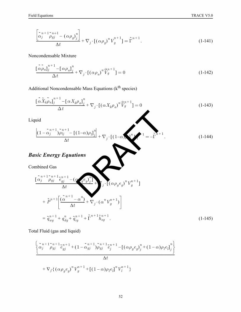
Field Equations TRACE V5.0
. (1-141)
Noncondensable Mixture
(1-142)
Additional Noncondensable Mass Equations (kth species)
(1-143)
Liquid
. (1-144)
Basic Energy Equations
Combined Gas
+
= . (1-145)
Total Fluid (gas and liquid)
+
αjn 1+
ρgjn+1
αρg( )jn –
t∆-------------------------------------------------------- ∇j αρg( )nVg
n 1+[ ]·+ Γ
n 1+=
αρa[ ]jn 1+
αρa[ ]jn–
∆t----------------------------------------------- ∇j αρa( )nVg
n 1+[ ]·+ 0=
αXkρa[ ]jn 1+
αXkρa[ ]jn–
∆t-------------------------------------------------------------- ∇j αXkρa( )nVg
n 1+[ ]·+ 0=
1 α– jn 1+
( )ρljn 1+
1 α–( )ρl[ ]jn–
t∆----------------------------------------------------------------------------- ∇j 1 α–( )ρl[ ]nVl
n 1+·+ Γ–n 1+
=
αjn 1+
ρgjn 1+
egjn 1+ αρgeg( )j
n–[ ]
t∆------------------------------------------------------------------------- ∇j αρgeg( )nVg
n 1+[ ]·+
Pn 1+ α
n 1+αn–( )
t∆------------------------------- ∇j αnVg
n 1+( )·+
qwgn 1+ qdg
n qign 1+ Γ
n 1+hsg
n 1++ ++
αjn 1+
ρgjn 1+
egjn 1+ 1 αgj
n 1+–( )ρgj
n 1+ejn 1+ αρgeg( )j
n 1 α–( )ρlel+[ ]jn
–+⎩ ⎭⎨ ⎬⎧ ⎫
t∆--------------------------------------------------------------------------------------------------------------------------------------------------------------------------------
· αρgeg( )nVgn 1+ 1 α–( )ρlel[ ]nVl
n 1++ j∇
DRAFT
52

TRACE V5.0 Field Equations
Field E
quations
+
= . (1-146)
The divergence operator is revised during the semi-implicit step to improve modeling accuracy ofsituations in which flux can be predominately attributed to phase change in the cell for which thecontinuity equation is being evaluated. The idea is to use new-time information for that portion ofthe flux associated with the same cell as the equation (cell ). This makes the local solution moresensitive to variation in phase-change rates. In terms of the notation used for the basic definitionof the divergence operator, the revised form is
. (1-147)
The special feature of this operator is that all occurrences of in the normal finite volumedivergence operator are replaced by a mixed time average defined as
. (1-148)
The weighting factor is determined by several considerations. For flow that is single phase overthe entire time step, is set to zero. When the net predicted flow out of a cell of either phaseexceeds the current mass in that cell, the weight is set to one (new-time cell-centered quantitiesare fluxed). For less dramatic situations, three ratios are computed. The first ratio has as anumerator the sum of the change in cell vapor mass for the time step due to all mass fluxes plustwice the change due to boiling. The ratio’s denominator is the cell’s mass decrease due only tooutwardly directed vapor mass flows (positive number). The second ratio is the analog of the firstas applied to the liquid phase. For the third ratio, the numerator adds half the old-time cell liquidmass to the predicted change in cell liquid mass for the time step. The denominator is half of themass change due to outwardly directed flows at the cell’s edges (negative number). When otherconsiderations are not in control, the maximum of the three ratios is limited to the range of zerothrough one and is used for γ.
The ratios used to compute the weighting factor were obtained after a long period ofexperimentation with two-phase-flow problems. The first two ratios force the use of a cell-centered implicit value when outflow of a phase is almost exclusively the result of phase-changeterms. The factor will also force this implicit evaluation when phase change is not significant andinflow significantly exceeds the outflow. The third ratio becomes important when some liquidoutflow is present and a prediction is made that over half of the existing liquid mass will flow orboil away during the time step.
Pn 1+ ∇j 1 α–( )nVl
n 1+ αnVgn 1++[ ]·
qwgn 1+ qwl
n 1+ qdln qdg
n+ ++
j
∇j˜ YnVg
n 1+( )·
wj 1 2⁄+
Yj′ 1 w
j 1 2⁄+–⎝ ⎠
⎛ ⎞ Yj 1+n+ A
j 1 2⁄+V
j 1 2⁄+w
j 1 2⁄–Yj 1–
n 1 wj 1 2⁄–
–⎝ ⎠⎛ ⎞ Yj
′+⟨ ⟩Aj 1 2⁄–
Vj 1 2⁄–
–
volj--------------------------------------------------------------------------------------------------------------------------------------------------------------------------------------------------------------------------------------------------------
=
Y'i
Yj′ γYj
n 1+ 1 γ–( )Yjn+=
γγ DRAFT
53

Field Equations TRACE V5.0
The mixture of old- and new-time values of the quantity being fluxed results in a differencescheme for this step that is not rigorously conservative. However, the standard finite-volumedivergence operator is applied in the stabilizer mass and energy equations, restoring conservationto the final fluxes of mass and energy.
To understand the stabilizer mass and energy equations, it is important to remember what isunknown and what quantities have fixed values. In this respect, the superscript “ ” can bedeceptive. New-time velocity values are fixed by the semi-implicit step, as are all new-time termsmarked with a tilde. In the stabilizer combined-gas mass equation, the only unknown new-time
variables are the macroscopic gas densities . For the noncondensable mass equation,
the only unknowns are the terms , and for the liquid mass equation, the only unknowns
are the terms . In the stabilizer combined-gas energy equation, the only unknown
new-time variables are the macroscopic gas energy densities . For the liquid energy
equation, the only unknowns are the terms .
Stabilizer Mass Equations
Combined Gas
. (1-149)
Noncondensable Gas
. (1-150)
Additional Noncondensable Mass Equations (kth species)
(1-151)
Liquid
. (1-152)
Liquid Solute (see the semi-implicit section for a description)
n 1+
αρg( )n 1+
αρa( )n 1+
1 α–( )ρl[ ]n 1+
αρgeg( )n 1+
1 α–( )ρlel[ ]n 1+
αρg( )jn 1+ αρg( )j
n–[ ]
t∆---------------------------------------------------- ∇j αρg( )n 1+ Vg
n 1+[ ]·+ Γjn 1+
=
αρa( )jn 1+ αρa( )j
n–[ ]
t∆---------------------------------------------------- ∇j αρa( )n 1+ Vg
n 1+[ ]·+ 0=
αXkρa[ ]jn 1+ αXkρa[ ]j
n–∆t
-------------------------------------------------------------- ∇j αXkρa( )n 1+ Vgn 1+
[ ]·+ 0=
1 α–( )ρl[ ]jn 1+ 1 α–( )ρl[ ]j
n–t∆
------------------------------------------------------------------------- ∇j 1 α–( )ρl[ ]n 1+ Vln 1+· ·+ Γj
n 1+–=
DRAFT
54

TRACE V5.0 Field Equations
Field E
quations
(1-153)
, (1-154)
and
. (1-155)
Stabilizer Energy Equations
Combined Gas
+
= . (1-156)
Liquid
+
= . (1-157)
As indicated in Enhancements to the SETS Method, the code does not directly solve all of theabove stabilizer equations. The actual equations solved are differences between these equationsand their corresponding equations from the semi-implicit step. For the case of solute transport, nocorresponding equation exists in the semi-implicit step. As a result, the stabilizer solute-transportequation, Eq. (1-154), is solved exactly as listed above. The final forms of the other equations asset in TRACE follow:
1 α–( )jn 1+ mj
n 1+ ρljn 1+ 1 α–( )j
nmjnρlj
n–[ ]t∆
----------------------------------------------------------------------------------------------------- ∇j 1 α–( )n 1+ mn 1+ ρln 1+ Vl
n 1+·+ 0=
mjn 1+ min mj
n 1+ Scjn
1 α–( )jn 1+ ρlj
n 1+---------------------------------------- , mmax+=
Scjn 1+ mj
n 1+ mjn 1+–( ) 1 α–( )j
n 1+ ρljn 1+ Scj
n+=
αρgeg( )jn 1+ αρgeg( )j
n–[ ]
t∆--------------------------------------------------------------- ∇j αρgeg( )n 1+ Vg
n 1+[ ]·+
Pjn 1+ αj
n 1+αj
n–( )t∆
------------------------------- ∇j αnVgn 1+( )·+
qwgn 1+ qdg
n qign 1+ Γj
n 1+hsg
n 1++ ++
1 α–( )ρlel[ ]jn 1+ 1 α–( )ρlel[ ]j
n–t∆
---------------------------------------------------------------------------------- ∇j 1 α–( )ρlel[ ]n 1+ Vln 1+ ·+
Pjn 1+ αj
n αjn 1+
–( )t∆
------------------------------- ∇j 1 α–( )nVln 1+[ ]·+
⎩ ⎭⎨ ⎬⎧ ⎫
qwln 1+ qdl
n qign 1+– Γj
n 1+hsg
n 1+–+
DRAFT
55

Field Equations TRACE V5.0
Stabilizer Mass Equations
Combined Gas
. (1-158)
Noncondensable Gas
. (1-159)
Additional Noncondensable Mass Equations (kth species)
(1-160)
Liquid
.
+ (1-161)
Stabilizer Energy Equations
Combined Gas
+ . (1-162)
Liquid
αρg( )jn 1+ αj
n 1+ρgj
n 1+–[ ]
t∆-------------------------------------------------------------- ∇j αρg( )n 1+ Vg
n 1+[ ]·+ ∇j αρg( )nVgn 1+[ ]·=
αρa( )jn 1+ αj
n 1+ρgj
n 1+–[ ]
t∆------------------------------------------------------------------ ∇j αρa( )n 1+ Vg
n 1+[ ]·+ ∇j αρa( )nVgn 1+[ ]·=
αXkρa[ ]jn 1+ αXkρa[ ]j
n 1+–∆t
--------------------------------------------------------------------- ∇j αXkρa( )n 1+ Vgn 1+
[ ]·+ ∇j αXkρa( )nVgn 1+
[ ]·=
1 α–( )ρl[ ]jn 1+ 1 α– j
n 1+( )ρlj
n 1+–
t∆-----------------------------------------------------------------------------------
∇j 1 α–( )ρl[ ]n 1+ Vln 1+ · ∇j 1 α–( )ρl[ ]nVl
n 1+ ·=
αρgeg( )jn 1+ αj
n 1+ρgj
n 1+egjn 1+–[ ]
t∆--------------------------------------------------------------------------------
∇j αρgeg( )n 1+ Vgn 1+[ ]· ∇j αρgeg( )nVg
n 1+[ ]·=
1 α–( )ρlel[ ]jn 1+ 1 αj
n 1+–( )ρlj
n 1+elj
n 1+–⎩ ⎭⎨ ⎬⎧ ⎫
t∆------------------------------------------------------------------------------------------------------------ ∇j 1 α–( )ρlel[ ]n 1+ Vl
n 1+ ·+
DRAFT
56

TRACE V5.0 Field Equations
Field E
quations
= . (1-163)
Source terms in the SETS equations follow the definitions provided during the discussion of thesemi-implicit methods. They are redefined below to clarify the use of intermediate variables.
, (1-164)
, (1-165)
and
, (1-166)
where
(1-167)
and
. (1-168)
As mentioned in Enhancements to the SETS Method, an important subtlety in the SETSapplication is the use of thermodynamic variables in the evaluation of specific terms. The currentform of the SETS solution provides only final new-time values for void fraction (α), macroscopic
densities , and macroscopic energies . A final call tothe thermodynamics equation-of-state does not occur after the solution of the stabilizer mass andenergy equations. As a result, when basic thermodynamic variables are needed for evaluation ofproperties such as viscosity or heat-transfer coefficients, values obtained from the previous semi-implicit step are used.
Eq. (1-134) and Eq. (1-136) do not involve any implicit coupling between cells and can be solveddirectly for the gas and liquid (caret) velocities at each mesh-cell interface. Eq. (1-137) andEq. (1-138) are not coupled to each other. Each of these systems is implicitly coupled in spacethrough the momentum-convection term, and each requires the solution of a tridiagonal linearsystem. Equations (1-139) through (1-146), combined with the necessary thermodynamic andconstitutive equations, form a coupled system of nonlinear equations. Eq. (1-139) and Eq. (1-140)
are solved directly to obtain and as linear functions of . After substitutingthese equations for velocity into Eqs. (1-141) through (1-146), the resulting system is solved with
∇j 1 α–( )ρlel[ ]nVln 1+ ·
qwln 1+ hwl
n aw Twn Tl
n 1+–( )=
qwgn 1+ hwg
n aw Twn Tg
n 1+–( )=
Γn 1+ qig
n 1+ qiln 1++⎝ ⎠
⎛ ⎞–
hv′( )
n 1+ hl′( )
n 1+–---------------------------------------------=
qign 1+ hig
n ain Tsat
n 1+T– g
n 1+( )=
qiln 1+ hil
nain Tsat
n 1+T– l
n 1+( )=
αρg αρa 1 α–( )ρl, ,[ ] αρgeg 1 α–( )ρlel,[ ]
Vgn 1+ Vl
n 1+ Pn 1+
DRAFT
57

Field Equations TRACE V5.0
a standard Newton iteration for the independent variables , , , ,
and any with , including all coupling between cells. In practice, the linearizedequations solved during this Newton iteration are reduced easily to a system is tridiagonal ordominately tridiagonal involving only total pressures. The final stabilizer mass and energyequations [Eq. (1-149) through Eq. (1-157)] also are simple tridiagonal linear systems because
and are known after solving Eq. (1-139) through Eq. (1-146).
3D Finite-Difference MethodsAll basic equations and stabilizer equations for the 3D VESSEL component are solved in thesame form as the 1D components. The vector form of the motion equation separates into threeorthogonal-coordinate velocity-component motion equations. We present only the combined-gasequations with the understanding that the liquid equations are treated analogously. The 3DVESSEL component can be modeled by the TRACE user in either cylindrical or Cartesiangeometry. The following equations in cylindrical geometry convert to Cartesian geometry by
replacing the divisor by unity and deleting the term in the divergence operator that
models momentum convection. The and dependence is replaced by x- and y-dependence. Foran orthogonal, right-handed, cylindrical coordinate system, the three velocity-component formsof the combined-gas motion differential equation are as follows:
Axial Velocity (z) Component
(1-169)
Radial Velocity (r) Component
. (1-170)
Azimuthal Velocity (θ) Component
Pn 1+ Pan 1+ Tg
n 1+ Tln 1+
αn 1+ Xk˜ n 1+ k 1>
Vgn 1+ Vl
n 1+
r V2 r⁄
r θ
Vgz∂
t∂------------ Vgr
Vgz∂
r∂------------
Vgθr
---------Vgz∂
θ∂------------ Vgz
Vgz∂
z∂------------+ +
⎝ ⎠⎜ ⎟⎜ ⎟⎛ ⎞
+ 1ρg-----
P∂
z∂-------– Γ+
αρg--------- Vgz Vlz–( )–=
Cizαρg--------- Vgz Vlz–( ) Vg Vl––
Cwgzαρg-----------Vgz Vg– ggz–
Vgr∂
t∂------------ Vgr
Vgr∂
r∂------------
Vgθr
---------Vgr∂
θ∂------------ Vgθ
2
r--------- Vgz
Vgr∂
z∂------------+–+
⎝ ⎠⎜ ⎟⎜ ⎟⎛ ⎞
+ 1ρg-----
P∂
r∂-------– Γ+
αρg--------- Vgr Vlr–( )–=
Cirαρg--------- Vgr Vlr–( ) Vg Vl––
Cwgrαρg------------Vgr Vg– ggr–
DRAFT
58

TRACE V5.0 Field Equations
Field E
quations
(1-171)
In the last term of each equation, is the gravitational acceleration constant and , , and are the directional components of the gravity vector based on the orientation of the 3D VESSEL
component. By default, TRACE internally defines , , and , where the z-axisis oriented vertically upward for all VESSEL components in the system model. The user may,however, redefine through input the orientation of each VESSEL component to something moregeneral.
TRACE uses a staggered-mesh scheme (Ref. 1-14) similar to that used for the 1D components inwhich the velocities ( ) are defined at the mesh-cell interfaces and the pressure ( ), gas volumefraction ( ), temperature ( ), internal energy ( ), and density ( ) are defined at the mesh-cellcenters. The scalar field equations (mass and energy) apply to a mesh cell, whereas the velocity-component motion equations apply to an interface between mesh cells in the three velocity-component directions. The wall heat transfer and the interfacial mass transfer required by the fieldequations are defined with a form similar to Eqs. (1-164) through (1-168).
The difference scheme for each motion equation is lengthy because of the cross-derivative terms.Therefore, to illustrate the procedure, we will describe only the combined-gas velocity-component, z-direction, finite-difference basic equation of motion for a typical mesh cellinterface, together with the gas basic mass and energy equations, for a typical mesh cell. The gasvelocity-component basic equations of motion in the and directions along with all of theliquid basic equations are similar in form. The stabilizer motion, mass, and energy equations willnot be illustrated; the reader is referred to the 1D component equations - Eq. (1-134) toEq. (1-146) and Eq. (1-149) to Eq. (1-163) - where time-level parameters with ˜, ˆ, , and superscripts are changed in going from the basic equations to the stabilizer equations. Thesuperscript indicates a current-time quantity; the superscript indicates a new-time
quantity. The functional dependence points to the cell center. By incrementing or
or by ±1, one moves to the adjacent cell in the direction based on which coordinate is
incremented and on the sign of the increment. The functional dependencies and
point to the inside and outside radial faces of the cell, respectively;
and , the right and left azimuthal faces of the cell (based on a
perspective of looking radially out of the cell), respectively; and and
Vgθ∂
t∂------------ Vgr
Vgθ∂
r∂------------
Vgθr
---------Vgθ∂
θ∂------------
VgrVgθr
------------------ VgzVgθ∂
z∂------------+ + +
⎝ ⎠⎜ ⎟⎜ ⎟⎛ ⎞
+ 1rρg--------
P∂
θ∂-------– Γ+
αρg--------- Vgθ Vlθ–( )–=
Ciθαρg--------- Vgθ Vlθ–( ) Vg Vl––
Cwgθαρg------------Vgθ Vg– ggθ–
g gz gr gθ
gz 1= gr 0= gθ 0=
V Pα T e ρ
θ r
n n 1+
n n 1+
r θ z, ,( ) r θz
r 1 2⁄– θ z, ,( )
r 1 2⁄+ θ z, ,( )
r θ 1 2⁄– z, ,( ) r θ 1 2⁄+ z, ,( )
r θ z 1 2⁄–, ,( )
DRAFT
59

Field Equations TRACE V5.0
, the bottom and top axial faces of the cell, respectively. The subscript (for gas)is dropped unless it is needed for clarity.
The finite-difference combined-gas basic equation of motion in the z-direction has the followingform:
Combined-Gas Basic Equation of Motion in the z-Direction
, (1-172)
r θ z 1 2⁄+, ,( ) g
Vzn 1+ r θ z 1 2⁄+, ,( ) Vz
n r θ z 1 2⁄+, ,( )=
∆tVr∆rVz
n 1+( )∆r
---------------------------------Vθ∆θVz
n 1+
r∆θ----------------------------- 1
2---
Az 1 2⁄+
Az 1+------------------
Az 1 2⁄+
Az------------------+
⎝ ⎠⎜ ⎟⎛ ⎞ Vz
n 1+ r θ z 1 2⁄+, ,( )∆z
-----------------------------------------------------+ +–
AZ 1 2⁄+
AZ 1+-------------------Vz
n 1+r θ Z 1 2⁄+, ,( )
AZ 1 2⁄–
AZ-------------------Vz
n 1+r θ Z 1 2⁄–, ,( )–
P r θ z 1+, ,( ) P r θ z, ,( )–[ ]n 1+
ρn r θ z 1 2⁄+, ,( )∆z----------------------------------------------------------------------------------–
Cizn r θ z 1 2⁄+, ,( )
α ρ,( )n
r θ z 1 2⁄+, ,( )---------------------------------------------------------–
Vg Vl–n Vgz Vlz–( )n r θ z 1 2⁄+, ,( )( )
2
Vg Vl–n
----------------------------------------------------------------------------+
⎩⎪⎨⎪⎧
× Vgz Vlz–( )n 1+ r θ z 1 2⁄+, ,( )
Vgz Vlz–( )n r θ z 1 2⁄+, ,( )( )
3
Vg Vl–n
----------------------------------------------------------------------------
⎭⎪⎬⎪⎫
–
Γ+n r θ z 1 2⁄+, ,( ) Vgz Vlz–( )n 1+ r θ z 1 2⁄+, ,( )
α ρ,( )n
r θ z 1 2⁄+, ,( )-----------------------------------------------------------------------------------------------------------------------------– ggz–
Cwzn r θ z 1 2⁄+, ,( ) Vg
n Vzn r θ z 1 2⁄+, ,( )( )
2
Vgn
-----------------------------------------------------+ Vzn 1+ r θ z 1 2⁄+, ,( )
Vzn r θ z 1 2⁄+, ,( )( )
3
Vgn
-----------------------------------------------------–
⎩ ⎭⎪ ⎪⎨ ⎬⎪ ⎪⎧ ⎫
α ρ,( )n
r θ z 1 2⁄+, ,( )-------------------------------------------------------------------------------------------------------------------------------------------------------------------------------------------------------------------------------------------------------–
DRAFT
60
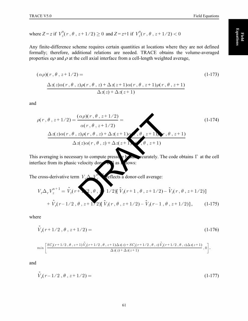
TRACE V5.0 Field Equations
Field E
quations
where Z = z if and Z = z+1 if
Any finite-difference scheme requires certain quantities at locations where they are not definedformally; therefore, additional relations are needed. TRACE obtains the volume-averagedproperties αρ and ρ at the cell axial interface from a cell-length weighted average,
(1-173)
and
(1-174)
This averaging is necessary to compute pressure heads accurately. The code obtains at the cellinterface from its phasic velocity donor cell as follows:
The cross-derivative term reflects a donor-cell average:
, (1-175)
where
(1-176)
.
and
(1-177)
Vzn r θ z 1 2⁄+, ,( ) 0≥ Vz
n r θ z 1 2⁄+, ,( ) 0<
αρ( ) r θ z 1 2⁄+, ,( )
∆z z( )α r θ z, ,( )ρ r θ z, ,( ) ∆z z 1+( )α r θ z 1+, ,( )ρ r θ z 1+, ,( )+∆z z( ) ∆z z 1+( )+
--------------------------------------------------------------------------------------------------------------------------------------------------------------------------
=
ρ r θ z 1 2⁄+, ,( )αρ( ) r θ z 1 2⁄+, ,( )
α r θ z 1 2⁄+, ,( )--------------------------------------------------
∆z z( )α r θ z, ,( )ρ r θ z, ,( ) ∆z z 1+( )α r θ z 1+, ,( )ρ r θ z 1+, ,( )+
∆z z( )α r θ z, ,( ) ∆z z 1+( )α r θ z 1+, ,( )+--------------------------------------------------------------------------------------------------------------------------------------------------------------------------
= =
Γ
Vr∆rVzn 1+
Vr∆rVzn 1+ Vr
˜ r 1 2⁄+ θ z 1 2⁄+, ,( ) Vz r 1+ θ z 1 2⁄+, ,( ) Vz r θ z 1 2⁄+, ,( )–[ ]=
Vr˜ r 1 2⁄– θ z 1 2⁄+, ,( ) Vz r θ z 1 2⁄+, ,( ) Vz r 1– θ z 1 2⁄+, ,( )–[ ]+
Vr˜ r 1 2⁄+ θ z 1 2⁄+, ,( ) =
min SCr r 1 2⁄+ θ z 1+, ,( )Vr
˜ r 1 2⁄+ θ z 1+, ,( )∆z z( ) SCr r 1 2⁄+ θ z, ,( )Vr˜ r 1 2⁄+ θ z, ,( )∆z z 1+( )+
∆z z( ) ∆z z 1+( )+--------------------------------------------------------------------------------------------------------------------------------------------------------------------------------------------------------------------------------------------------------------- 0,
Vr˜ r 1 2⁄– θ z 1 2⁄+, ,( ) =
DRAFT
61

Field Equations TRACE V5.0
.
In the above equations, “min” and “max” are the mathematical functions of minimum and
maximum values of the terms inside the brackets. is the product of an orificefactor that is 0 (when an orifice plate is present at the r+1/2 interface) or 1 and the ratio of the flow
area through the interface to the cell flow area in the radial direction,
. The oriface factor is simply a statement that transverse momentum is nottransported across an oriface. This assumption is particularly valid at the upper and lower coresupport plates. The area ratio contained in SC is consistent with the discussion later in this chapter
of use of area ratios in momentum flux terms. An analogous expression holds for the term.
Note that the differences in the r and θ directions do not contain the z-direction flow-area
weighting form. The and factors make this correction for z-direction momentum
convection in the and directions, respectively.
In the interfacial drag terms, the magnitude of the relative velocity is defined as follows:
+
−
+
− . (1-178)
The convective terms in the finite volume relations for the scalar field equations are inconservative form. The finite-difference form of the combined-gas basic mass equation is
max SCr r 1 2⁄– θ z 1+, ,( )Vr
˜ r 1 2⁄– θ z 1+, ,( )∆z z( ) SCr r 1 2⁄– θ z, ,( )Vr˜ r 1 2⁄– θ z, ,( )∆z z 1+( )+
∆z z( ) ∆z z 1+( )+-------------------------------------------------------------------------------------------------------------------------------------------------------------------------------------------------------------------------------------------------------------- 0,
SCr r 1 2⁄+ θ z, ,( )
r 1 2⁄+ r θ z, ,( )
vol r θ z, ,( ) ∆rcell⁄
Vθ∆θVzn 1+
Vz
SCr SCθ
r θ
Vg Vl– Vzg r θ z 1 2⁄+, ,( ) Vzl r θ z 1 2⁄+, ,( )–[ ]2
⎩⎨⎧
=
0.25 Vrg r 1 2 θ z, ,⁄+( ) Vrg r 1 2 θ z, ,⁄–( )+([
Vrl r 1 2⁄ θ z, ,+( ) Vrl r 1 2⁄ θ z, ,–( )– ]2
0.25 Vθg r θ 1 2⁄ z,+,( ) Vθg r θ 1 2⁄ z,–,( )+[
Vθl r θ 1 2⁄ z,+,( ) Vθl r θ 1 2⁄ z,–,( )– ]2
⎭⎬⎫1 2⁄
DRAFT
62
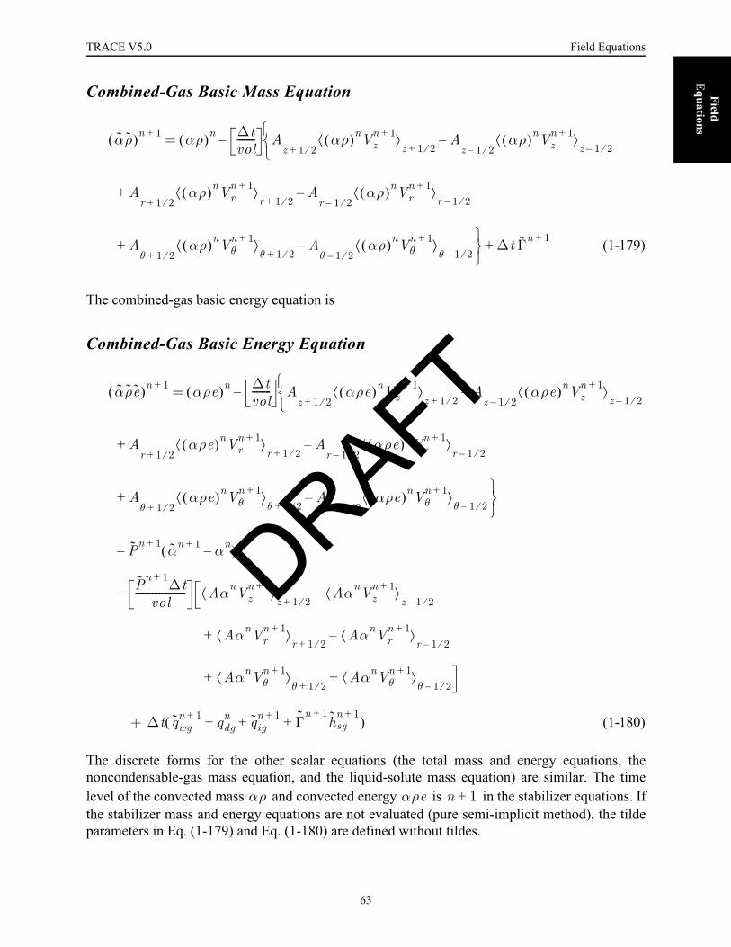
TRACE V5.0 Field Equations
Field E
quations
Combined-Gas Basic Mass Equation
(1-179)
The combined-gas basic energy equation is
Combined-Gas Basic Energy Equation
(1-180)
The discrete forms for the other scalar equations (the total mass and energy equations, thenoncondensable-gas mass equation, and the liquid-solute mass equation) are similar. The timelevel of the convected mass and convected energy is in the stabilizer equations. Ifthe stabilizer mass and energy equations are not evaluated (pure semi-implicit method), the tildeparameters in Eq. (1-179) and Eq. (1-180) are defined without tildes.
αρ( )n 1+ αρ( )n ∆tvol-------- A
z 1 2⁄+αρ( )nVz
n 1+⟨ ⟩z 1 2⁄+
Az 1 2⁄–
αρ( )nVzn 1+⟨ ⟩
z 1 2⁄––
⎩⎨⎧
–=
Ar 1 2⁄+
αρ( )nVrn 1+⟨ ⟩
r 1 2⁄+A
r 1 2⁄–αρ( )nVr
n 1+⟨ ⟩r 1 2⁄–
–+
Aθ 1 2⁄+
αρ( )nVθn 1+⟨ ⟩
θ 1 2⁄+A
θ 1 2⁄–αρ( )nVθ
n 1+⟨ ⟩θ 1 2⁄–
–⎭⎬⎫
∆t Γn 1++ +
αρe( )n 1+ αρe( )n ∆tvol-------- A
z 1 2⁄+αρe( )nVz
n 1+⟨ ⟩z 1 2⁄+
Az 1 2⁄–
αρe( )nVzn 1+⟨ ⟩
z 1 2⁄––
⎩⎨⎧
–=
Ar 1 2⁄+
αρe( )nVrn 1+⟨ ⟩
r 1 2⁄+A
r 1 2⁄–αρe( )nVr
n 1+⟨ ⟩r 1 2⁄–
–+
Aθ 1 2⁄+
αρe( )nVθn 1+⟨ ⟩
θ 1 2⁄+A
θ 1 2⁄–αρe( )nVθ
n 1+⟨ ⟩θ 1 2⁄–
–⎭⎬⎫
+
Pn 1+ αn 1+ αn–( )–
Pn 1+ ∆tvol
--------------------- AαnVzn 1+⟨ ⟩
z 1 2⁄+AαnVz
n 1+⟨ ⟩z 1 2⁄–
–
AαnVrn 1+⟨ ⟩
r 1 2⁄+AαnVr
n 1+⟨ ⟩r 1 2⁄–
–
AαnVθn 1+⟨ ⟩
θ 1 2⁄+AαnVθ
n 1+⟨ ⟩θ 1 2⁄–
+
+ +
–
+ ∆t qwgn 1+ qdg
n qign 1+ Γ
n 1+hsg
n 1++ + +( )
αρ αρe n 1+
DRAFT
63
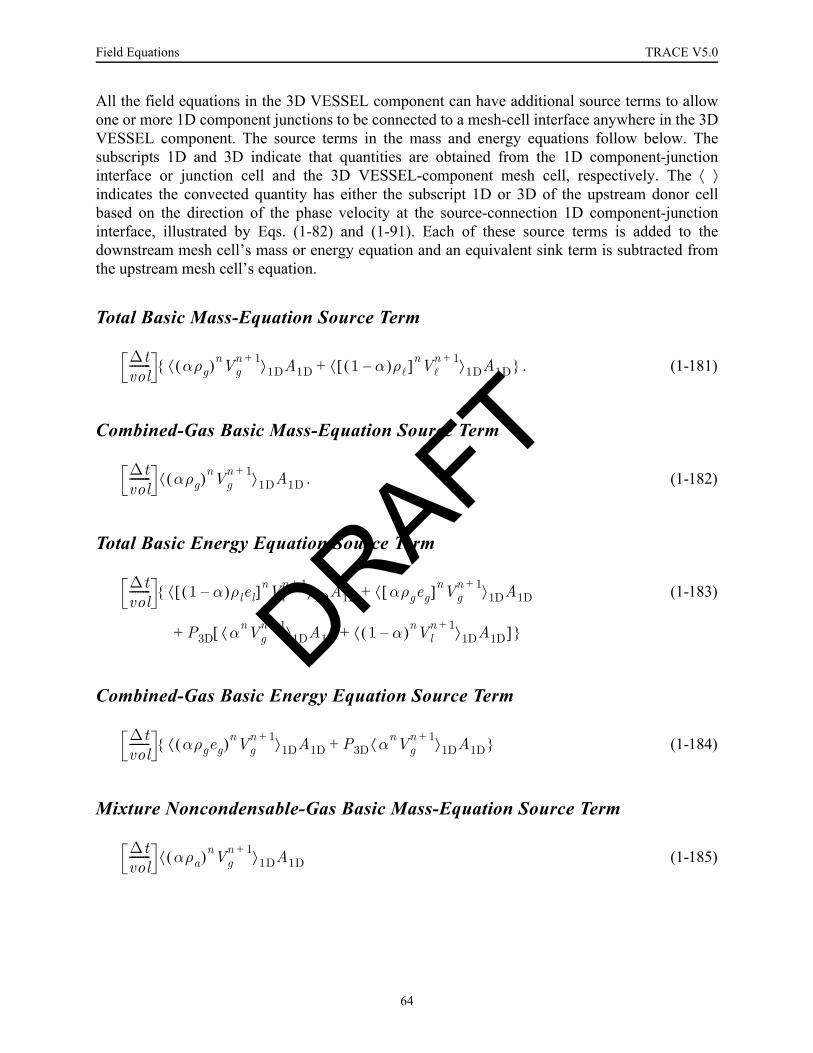
Field Equations TRACE V5.0
All the field equations in the 3D VESSEL component can have additional source terms to allowone or more 1D component junctions to be connected to a mesh-cell interface anywhere in the 3DVESSEL component. The source terms in the mass and energy equations follow below. Thesubscripts 1D and 3D indicate that quantities are obtained from the 1D component-junctioninterface or junction cell and the 3D VESSEL-component mesh cell, respectively. The ⟨ ⟩indicates the convected quantity has either the subscript 1D or 3D of the upstream donor cellbased on the direction of the phase velocity at the source-connection 1D component-junctioninterface, illustrated by Eqs. (1-82) and (1-91). Each of these source terms is added to thedownstream mesh cell’s mass or energy equation and an equivalent sink term is subtracted fromthe upstream mesh cell’s equation.
Total Basic Mass-Equation Source Term
. (1-181)
Combined-Gas Basic Mass-Equation Source Term
. (1-182)
Total Basic Energy Equation Source Term
(1-183)
Combined-Gas Basic Energy Equation Source Term
(1-184)
Mixture Noncondensable-Gas Basic Mass-Equation Source Term
(1-185)
∆tvol-------- αρg( )nVg
n 1+⟨ ⟩1DA1D 1 α–( )ρl[ ]nVln 1+⟨ ⟩1DA1D+
∆tvol-------- αρg( )nVg
n 1+⟨ ⟩1DA1D
∆tvol-------- 1 α–( )ρlel[ ]nVl
n 1+⟨ ⟩1DA1D αρgeg[ ]nVgn 1+⟨ ⟩1DA1D
P3D αnVgn 1+⟨ ⟩1DA1D 1 α–( )nVl
n 1+⟨ ⟩1DA1D+[ ]
+
+
∆tvol-------- αρgeg( )nVg
n 1+⟨ ⟩1DA1D P3D αnVgn 1+⟨ ⟩1DA1D+
∆tvol-------- αρa( )nVg
n 1+⟨ ⟩1DA1D
DRAFT
64
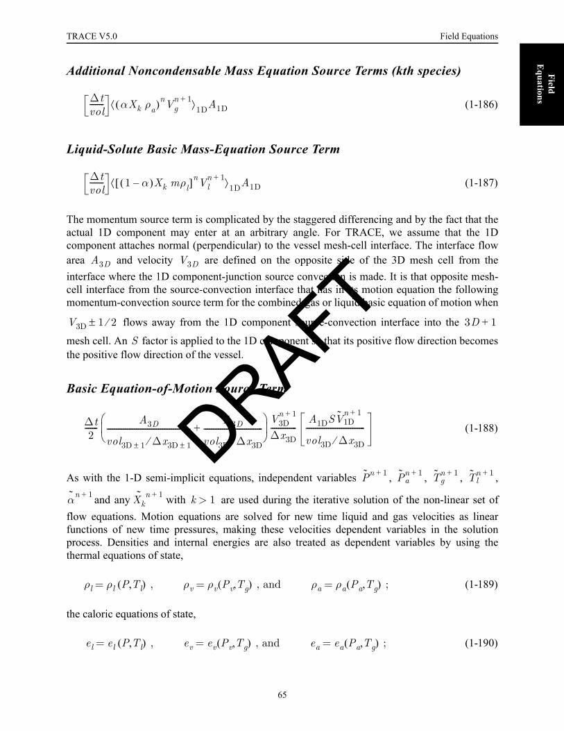
TRACE V5.0 Field Equations
Field E
quations
Additional Noncondensable Mass Equation Source Terms (kth species)
(1-186)
Liquid-Solute Basic Mass-Equation Source Term
(1-187)
The momentum source term is complicated by the staggered differencing and by the fact that theactual 1D component may enter at an arbitrary angle. For TRACE, we assume that the 1Dcomponent attaches normal (perpendicular) to the vessel mesh-cell interface. The interface flowarea and velocity are defined on the opposite side of the 3D mesh cell from theinterface where the 1D component-junction source convection is made. It is that opposite mesh-cell interface from the source-convection interface that has in its motion equation the followingmomentum-convection source term for the combined-gas or liquid basic equation of motion when
flows away from the 1D component source-convection interface into the
mesh cell. An factor is applied to the 1D component so that its positive flow direction becomesthe positive flow direction of the vessel.
Basic Equation-of-Motion Source Term
(1-188)
As with the 1-D semi-implicit equations, independent variables , , , ,
and any with are used during the iterative solution of the non-linear set offlow equations. Motion equations are solved for new time liquid and gas velocities as linearfunctions of new time pressures, making these velocities dependent variables in the solutionprocess. Densities and internal energies are also treated as dependent variables by using thethermal equations of state,
(1-189)
the caloric equations of state,
(1-190)
∆tvol-------- αXk ρa( )nVg
n 1+⟨ ⟩1DA1D
∆tvol-------- 1 α–( )Xk mρl[ ]nVl
n 1+⟨ ⟩1DA1D
A3D V3D
V3D 1 2⁄± 3D 1+
S
∆t2
-------A3D
vol3D 1± ∆x3D 1±⁄---------------------------------------------
A3D
vol3D ∆x3D⁄--------------------------------+
⎝ ⎠⎜ ⎟⎛ ⎞ V3D
n 1+
∆x3D--------------
A1DSV1Dn 1+
vol3D ∆x3D⁄--------------------------------
Pn 1+ Pan 1+ Tg
n 1+ Tln 1+
αn 1+ Xk˜ n 1+ k 1>
ρl ρl P Tl( , ) , ρv ρv Pv Tg( , ) , and ρa ρa Pa Tg( , ) ;= = =
el el P Tl( , ) , ev ev Pv Tg( , ) , and ea ea Pa Tg( , ) ;= = =
DRAFT
65

Field Equations TRACE V5.0
and the definitions for , , and P (Eqs. , (1-42) through (1-45)).
If one or more hardware structures exist in the 3D mesh cells, the interface flow area ( ) for fluidflow and the mesh-cell fluid volume ( ) are reduced from their geometric mesh-cell values bythe user through inputting fractions of their geometric area and volume. These fractions can beinput with values greater than unity, but it is recommended that the user not do so for the model tobe physically valid. Thus, should be less than or equal to the geometric mesh-cell side area and“ ” should be less than or equal to the geometric mesh-cell volume. Mesh-cell fluid volumes
are constrained to be by TRACE. When the flow area is defined to be zero, fluidflow across the mesh-cell interface is zero. This procedure allows large obstacles, such as thedowncomer walls and flow channels, to be modeled within the VESSEL component.
Modifications to the Basic Equation SetBecause of the choice of independent variables in the solution of the 1D or 3D basic equations(total pressure, air partial pressure, void fraction, combined-gas and liquid temperatures, and massfractions of any noncondensable species beyond the first), the basic equation set becomes singularat void fractions of zero and one. To avoid this solution difficulty the combined gas mass equation
(1-141). is replaced with a simple equation setting or . The combined-gas energyequation is replaced with an equation setting the temperature of the missing phase to thesaturation temperature based on the total pressure.
When the transition from single-phase gas or liquid to a two-phase fluid first occurs, thecombined-gas and liquid mass equations are evaluated but the replacement equation for the gasenergy equation is used for one more time step. This forces the second phase to initially appear atsaturation conditions, which is generally a very good approximation. It drastically reducessporadic numerical problems associated with the use of two energy equations in which the firstappearance of a phase can be associated with an exceptionally bad predicted value of itstemperature. Special considerations are also made during the linearization for the Newtonsolution of the semi-implicit equations. When an explicit mass test suggests the first appearanceof a second phase, flux of the second phase is used to estimate the new-time void fraction. If air isjust appearing in a cell, an initial estimate is also made of the air partial pressure. Both of theseestimates are used to specify the base state for the linearization associated with the currentNewton iteration.
When the pressure exceeds the critical-point pressure, the basic equations can become singular.However, care has been taken to place a minimum value on the difference between liquid andvapor density wherever it appears in a constitutive equation. This results in a two-phase equationset that drives itself rapidly to single phase when pressure is above the critical point.
ρg eg
Avol
Avol
1 12–×10 m3≥
α 0= α 1=
DRAFT
66

TRACE V5.0 Field Equations
Field E
quations
Conserving Convected Momentum
The backward difference approach given in Eq. (1-85) to determine the term in amomentum equation is known to be stable numerically. For smooth area changes, however, thisbackward or upwind difference scheme is not accurate and does not conserve momentum. Forabrupt area changes, it can be shown that the upwind difference scheme combining Eq. (1-85) and
Eq. (1-91) for will result in pressure changes that include both reversible and irreversibleeffects. Upwind differencing is accurate for abrupt expansions and overestimates the pressurechange for an abrupt contraction. (see Chapter 7, Form Loss Models for details.)
It has been shown that the accuracy of a central difference representation of is quite goodfor smooth area changes and for the reversible portion of an abrupt area change. It can be shown,however, through linear stability analysis, that central differencing is, in general, unconditionallyunstable. An approach was developed (originally for TRAC-PF1/MOD2 and carried over intoTRACE) to improve momentum conservation by determining factors based on geometry that
change the upwind differencing of the so that its accuracy is consistent with centraldifferencing. The assumption used in developing these factors is constant volumetric flow fromthe cell center to the cell edge.
A central difference for 1D flow yields
. (1-191)
Equation (1-191) can be rewritten as
(1-192)
In TRACE, velocities are calculated at cell edges, therefore cell-center velocities must beestimated from cell-edge velocities. Equation (1-192) can be written in terms of the cell-edgevelocities by applying the following equations based on constant volumetric flow from cell centerto the cell edge:
, (1-193)
, (1-194)
V V∇·
V V∇·
V V∇·
V V∇·
V V∇·
V V∇·V Vd
xd------------
0.5 V 2( )d
xd------------------------
0.5 Vj 1+2 Vj
2–( )∆x
j 1 2⁄+
--------------------------------------≡= =
V V∇·0.5 Vj 1+ Vj+( ) Vj 1+ Vj–( )
∆xj 1 2⁄+
-------------------------------------------------------------------=
Aj 1+ Vj 1+ Aj 1 2⁄+
Vj 1 2⁄+
=
AjVj Aj 1 2⁄+
Vj 1 2⁄+
=
DRAFT
67

Field Equations TRACE V5.0
and
. (1-195)
If Eqs. (1-193) and (1-194) are substituted into the summed portion of Eq. (1-192), and Eqs.(1-193) and (1-195) are substituted into the difference portion of Eq. (1-192), an upwind
difference form that is as accurate as central differencing is obtained for .
(1-196)
These equations assume that but similar sets of equations can be derived for
. In TRACE, Eq. (1-196) is the approximation used in both the 1D and 3D
momentum-convection terms to improve the conservation of momentum.
In general, TRACE, even with the corrected term, is still solving a nonconservingmomentum equation. What follows is a simplified version of the derivation leading to Eq. (1-78).A conserving form of the momentum equation for single-phase flow with no momentum sourcesor sinks can be written as
(1-197)
Expanding the derivatives of Eq. (1-197) yields
. (1-198)
The continuity equation for single-phase flow with no sources or sinks can be written as
(1-199)
Therefore, Eq. (1-198) can be written as
AjVj Aj 1 2⁄–
Vj 1 2⁄–
=
V V∇·
V V∇·j 1 2⁄+
0.5A
j 1 2⁄+
Aj 1+------------------
Aj 1 2⁄+
Aj------------------+
⎝ ⎠⎜ ⎟⎛ ⎞
Vj 1 2⁄+
Aj 1 2⁄+
Vj 1 2⁄+
Aj 1+-------------------------------------
Aj 1 2⁄–
Vj 1 2⁄–
Aj------------------------------------–
⎝ ⎠⎜ ⎟⎛ ⎞
∆xj 1 2⁄+
-----------------------------------------------------------------------------------------------------------------------------------------------------------------=
Vj 1 2⁄+
0≥
Vj 1 2⁄+
0<
V V∇·
d ρV( )dt
---------------- d ρVAV( )
A xd------------------------- 0= =
Vρ( )d
td-----------
ρVA( )d
A xd--------------------+
⎩ ⎭⎨ ⎬⎧ ⎫
ρV( )d
td------------ V
V( )d
xd------------+
⎩ ⎭⎪ ⎪⎨ ⎬⎪ ⎪⎧ ⎫
+ 0=
d ρ( )dt
----------- d ρVA( )Adx
---------------------+ 0=
DRAFT
68

TRACE V5.0 Field Equations
Field E
quations
. (1-200)
Equation (1-200) represents the type of nonconserving form of the momentum equation solved bythe TRACE code. This derivation indicates that TRACE will conserve momentum with thenonconserving form of the momentum equation if mass is conserved on a point-by-point basis.TRACE conserves mass within each hydraulic cell and assumes that within that cell, the densityand void fractions are constant. This assumption may lead to errors in conserving momentum,since the nonconserving momentum equation is solved from cell center to cell center and thegeometry area ratio factors developed for Eq. (1-196) assume constant density and void fractionfrom cell center to cell edge.
If we assume constant volumetric flow from cell edge j−1/2 to cell edge j+1/2, Eq. (1-196) in theform of the Bernoulli equation is equivalent to
. (1-201)
Substitute the constant volumetric-flow relations and
into the momentum-convection term of Eq. (1-201) to obtain the
Bernoulli equation
. (1-202)
We see from the above derivation of the momentum-convection term and the assumptions madethat the equation of motion for single-phase liquid (a near-incompressible fluid) to a very goodapproximation satisfies the Bernoulli equation. Convected momentum flux between momentumcells should be nearly conserved. Reversible form losses caused by flow-area and elevationchanges should be evaluated correctly. This has been demonstrated (Ref. 1-15) for single-phaseliquid with a variable flow-area and elevation flow-channel test problem having a total of seven1D PIPE and VESSEL components connected in series with a FILL-component velocity andBREAK-component pressure boundary condition at each end of the flow channel, respectively.Each 1D VESSEL component was evaluated in each of three Cartesian-coordinate directions in
separate calculations. Wall losses in the flow channel with flow area varying from 0.1 to 0.6 were minimized by increasing the flow-channel hydraulic diameter by a factor of 100.
A plot of the Bernoulli expression (as calculated using TRAC-PF1/MOD2)
versus flow-channel cell number for four different PIPE- and VESSEL-component models is
V( )d
td----------- V
V( )dxd
-----------+ 0=
Pj 1+ Pj– ρ2---
Aj 1 2⁄+
Aj 1+------------------V
j 1 2⁄+⎝ ⎠⎜ ⎟⎛ ⎞
2 Aj 1 2⁄–
Aj------------------V
j 1 2⁄–⎝ ⎠⎜ ⎟⎛ ⎞
2
– ρg∆xj 1 2⁄+
θcos+ + 0=
Aj 1 2⁄+
Vj 1 2⁄+
Aj 1+ Vj 1+=
Aj 1 2⁄–
Vj 1 2⁄–
AjVj=
Pj 1+ Pj– 12---ρ Vj 1+
2 Vj2–[ ] ρg∆x
j 1 2⁄+θcos+ + 0=
m2
Pj ρj⁄ Vj2 2⁄ ghj+ +
j
DRAFT
69

Field Equations TRACE V5.0
shown in Figure 1-7, with and without flow-area ratios applied in the momentum-convection termof the liquid equation of motion. Each of the four models comprised a different combination ofPIPE and/or 1D VESSEL components, yet each gave the same results. The momentum equationcurrently used in TRACE provided an accurate evaluation of the Bernoulli equation asdemonstrated by the constant value of the Bernoulli expression when flow-area ratios are appliedin the momentum-convection term. Similar calculations were performed for single-phase vaporwherein TRAC-PF1/MOD2 was temporarily modified to evaluate a constant vapor microscopicdensity (making vapor an incompressible fluid). The results determined were similar to those ofliquid, which served as a check that the combined-gas equation of motion as well as the liquidequation of motion are programmed correctly for both 1D and 3D components.
For a compressible single-phase vapor, the change in its microscopic density because of fluidpressure and temperature variation over a mesh-cell distance generally is small. Approximatingconstant density within a fluid cell should cause only a small error in conserving convected vapormomentum flux between momentum cells. However, a significant spatial variation in the fluidvoid fraction across a mesh cell can result in a momentum-flux conservation error, in part becauseof the constant volumetric-flow assumption. However, for rapidly changing void fractions thelarger problem in momentum conservation can be traced to the assumption equating two differentaverages of macroscopic density, leading to the difference between Eq. (1-76) and Eq. (1-77).
Figure. 1-7. The Bernoulli expression Pj / ρj + Vj2 / 2 + ghj vs. flow-channel
cell number j from a 1D flow-channel test problem having variable flow area and elevation. This calculation was performed with TRAC-PF1/MOD2.
1025
1020
1015
1010
10050 5 10 15 20
Cell Number
With Flow-Area Ratios
Single-Phase LiquidDH Times 100
Without Flow-Area Ratios
1025
1020
1015
1010
10050 5 10 15 20
With Flow-Area Ratios
Single-Phase Liquid
Without Flow-Area Ratios
P/ρ
+ V
2 /2 +
gh
(m2 /s
2 )
DRAFT
70

TRACE V5.0 Field Equations
Field E
quations
Reversible and Irreversible Form Losses.
With flow-area ratios in the momentum-convection term, TRACE approximately conservesconvected momentum and evaluates only the reversible form losses of the Bernoulli equation.The TRACE user is therefore responsible for supplying input that specifies all irreversible formlosses due to abrupt or semi-abrupt flow-area expansions and contractions, thin-plate-orifice-typeflow restrictions, and flow redirection (turning) at an elbow or tee, as discussed in Chapter 7,Form Loss Models.
TRACE users who are adapting old TRAC-PF1/MOD1 input files need to be aware of a conflictin the way form losses are applied between TRACE and that older code. The TRAC-PF1/MOD1momentum-convection term does not include the flow-area ratios illustrated in Eq. (1-196). Thatresults in a numerically produced irreversible form loss that is about right for an abrupt expansionand approximately twice the irreversible form loss of an abrupt contraction. Code users who haveprepared TRAC-PF1/MOD1 input-data plant models have compensated for this numericallygenerated irreversible form-loss error by not including other irreversible form losses at flowrestrictions or at elbows and tees in order to evaluate the correct overall pressure drop through aportion or all of a flow loop. TRACE users who inherit and convert such TRAC-PF1/MOD1input-data files into TRACE input-data files need to be aware that their plant model may havebuilt-in compensating-error features for TRAC-PF1/MOD1 that, when evaluated by TRACE,give pressure losses along flow paths that are significantly low. The user’s response to thissituation should be to never use converted TRAC-PF1/MOD1 input-data files blindly. All mesh-cell interface flow areas and mesh-cell volumes and lengths (whose ratio defines mesh-cell flowarea) need to be checked against plant specifications, and all input-specified FRICs or K-factors(and those that have not been specified) need to be defined to account for their actual irreversibleform losses at abrupt or semi-abrupt flow-area changes, flow restrictions, and flow turns(redirections).
TRACE assists code users by not requiring them to determine values loss coefficients at abruptexpansion or contraction 1D component mesh-cell interfaces for input specification. At all suchinterfaces, TRACE internally evaluates the standard K-factor formulas in Chapter 7, Form LossModels, for abrupt-expansion [K = (1−Amin/Amax)2] and abrupt-contraction [K = 0.5 − 0.7(Amin/Amax) + 0.2 (Amin/Amax)2] form losses based on mesh-cell flow areas and adds them to the anyinput-specified loss coefficients. This feature is extended in TRACE to 3D VESSEL componentsas well.
Special Cases
The definition of flow-area ratios and irreversible form losses when evaluating momentumconvection in BREAK, PLENUM, TEE (and, more generally, side junctions), and VESSELcomponents needs further consideration.
DRAFT
71

Field Equations TRACE V5.0
BREAK Component
TRACE models a BREAK component as a volume in which state conditions are prescribed by theuser rather than generated through the solution of flow equations. The user specifies the volumeof the cell and a characteristic length perpendicular to it’s connection area. A momentum equationis evaluated at the BREAK junction area, and when an area is required from the BREAK side foruse in the momentum transfer terms, it is obtained by dividing the BREAK volume by theBREAK characteristic length. TRACE user’s need to think carefully about the physicalconfiguration within which the BREAK is being used a a boundary condition to isolate asubsystem. If in the real system piping continues beyond BREAK junction, the pipe geometrymust be considered in setting the BREAK geometry. If piping ends at the BREAK junction andflow enters a very large volume (e.g. containment), the ratio of volume to length in the breakshould give an area much larger than the flow area at the BREAK junction. The characteristiclength input for the BREAK should not, however, be a characteristic length for the large physicalvolume. It is used in the pressure gradient term in the junction momentum equation, and should besmall to reflect the fact that pressure changes rapidly as it enters the large volume. The standardguideline for TRACE is to set the length for the BREAK equal to the length of the computationalvolume immediately adjacent to the BREAK.
As with other points of abrupt area change, when the flow area changes between the BREAKmesh cell and the adjacent-component mesh cell, we recommend user specification of anappropriate irrecoverable loss coefficient. This can be done either as a specific coefficient, or arequest that TRACE calculate an appropriate coefficient. It is important to provide a dissipativeterm in the equation of motion to determine the correct and numerically stable solution. ABREAK component is a pressure boundary condition that locally removes a degree of freedomfrom the hydrodynamic solution. The equation set becomes locally stiffer and more sensitive toerror growth when there is not a dissipative term.
PLENUM Component
In general, we no longer recommend use of the PLENUM component when developing newTRACE input models. We document it here for completeness in case you find yourselfmaintaining or using a legacy model that includes such a component type.
The PLENUM component is a single mesh cell with a user selected number of junction interfacesconnected to 1D components. Momentum can be transferred into a plenum but not across aplenum from one connecting face to another. The input for a plenum requests a characteristiclength associated with each connection. This can be considered as twice the distance from theconnecting face to the center of the plenum. When a plenum area is needed as part of themomentum transfer term, it is calculated as the ratio of plenum volume divided by thecharacteristic length associated with the junction at which the momentum equation is evaluated.When a velocity is needed from the plenum side for use in the momentum transfer term it is takento be zero. For example if face j+1/2 in Eq. (1-196) is a plenum junction, and volume j is theplenum, the equation becomes:
DRAFT
72
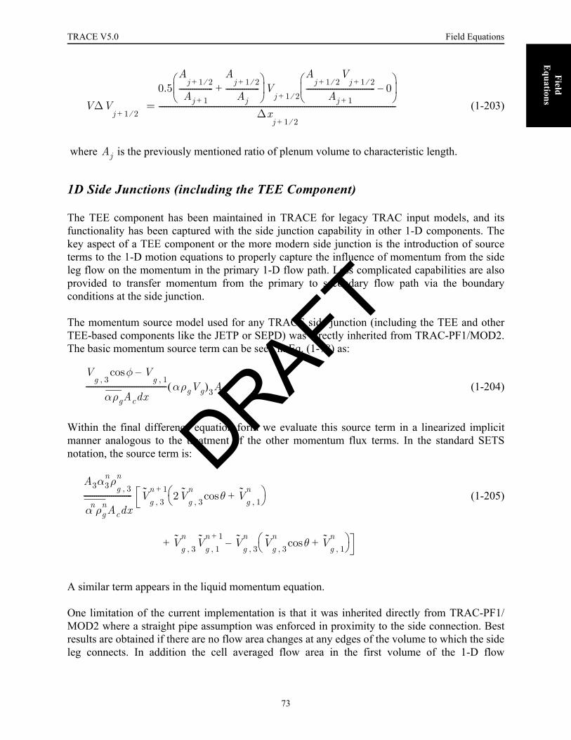
TRACE V5.0 Field Equations
Field E
quations
(1-203)
where is the previously mentioned ratio of plenum volume to characteristic length.
1D Side Junctions (including the TEE Component)
The TEE component has been maintained in TRACE for legacy TRAC input models, and itsfunctionality has been captured with the side junction capability in other 1-D components. Thekey aspect of a TEE component or the more modern side junction is the introduction of sourceterms to the 1-D motion equations to properly capture the influence of momentum from the sideleg flow on the momentum in the primary 1-D flow path. Less complicated capabilities are alsoprovided to transfer momentum from the primary to secondary flow path via the boundaryconditions at the side junction.
The momentum source model used for any TRACE side junction (including the TEE and otherTEE-based components like the JETP or SEPD) was directly inherited from TRAC-PF1/MOD2.The basic momentum source term can be seen in Eq. (1-78) as:
(1-204)
Within the final difference equation form we evaluate this source term in a linearized implicitmanner analogous to the treatment of the other momentum flux terms. In the standard SETSnotation, the source term is:
(1-205)
A similar term appears in the liquid momentum equation.
One limitation of the current implementation is that it was inherited directly from TRAC-PF1/MOD2 where a straight pipe assumption was enforced in proximity to the side connection. Bestresults are obtained if there are no flow area changes at any edges of the volume to which the sideleg connects. In addition the cell averaged flow area in the first volume of the 1-D flow
V∆Vj 1 2⁄+
0.5A
j 1 2⁄+
Aj 1+------------------
Aj 1 2⁄+
Aj------------------+
⎝ ⎠⎜ ⎟⎛ ⎞
Vj 1 2⁄+
Aj 1 2⁄+
Vj 1 2⁄+
Aj 1+------------------------------------- 0–
⎝ ⎠⎜ ⎟⎛ ⎞
∆xj 1 2⁄+
-------------------------------------------------------------------------------------------------------------------------------=
Aj
Vg 3,
φ Vg 1,
–cos
αρgAcdx------------------------------------------- αρgVg( )3A3
A3α3nρ
g 3,n
αnρgnAcdx
-------------------------- Vg 3,n 1+
2Vg 3,n θcos Vg 1,
n+⎝ ⎠
⎛ ⎞
Vg 3,n
Vg 1,n 1+
Vg 3,n
Vg 3,n θcos V
g 1,n
+⎝ ⎠⎛ ⎞–+
DRAFT
73

Field Equations TRACE V5.0
component connected to the side junction should be the same as the side junction’s area. Theserestrictions will be lifted with TRACE v6.0.
Differences in implementation of the momentum transport terms also affect irrecoverable losscoefficients. The option for automatic internal calculation of these coefficients is disabled at theedges of a volume containing a side junction. If area changes are present the code user needs tocarefully check that pressure drops through the primary flow path are acceptable. If more pressureloss is needed, then specific values of loss coefficients should be supplied via the input. If toomuch pressure loss is obtained adjacent to a junction volume, then renodalization may berequired.
A discussion of the side junction (TEE) model inherited from TRAC-PF1/MOD2 is given inReference 1-17.
VESSEL Component.
Using flow-area ratios to correctly donor-cell the approximate momentum flux at a mesh-cellcenter (based on its interface-defined velocity a half mesh-cell distance away) is done only formomentum that is convected by its own component-direction velocity. This is not done in thecross-derivative terms of the divergence operator for momentum convection as shown in Eqs.(1-176) and (1-177).
Flow-area ratios are evaluated using the mesh-cell average flow area, , where d = i,
j, or k defines the component direction of the equation of motion. When the structure volumefraction within a 3D mesh cell is nonuniform in the d direction, the average flow area for the mesh
cell can be incorrectly defined by . Nonphysical mesh-cell flow areas affect the
pressure solution through the Bernoulli equation by not approximating the donor-cell-approximated velocity components at the mesh-cell centers correctly. Locating 3D mesh-cellinterfaces on planes of structure volume-fraction discontinuity can minimize this modelingdifficulty. A modeling example that is difficult to handle correctly is representing the internalstructure curved surface of a pressure vessel that bisects mesh cells in the vessel lower plenum.
A source connection to a 3D VESSEL component by a 1D component uses the and ∆d
geometry parameters of the mesh cell (where refers to the edge direction to which the1-D flow is connected), to define the 3D mesh-cell flow area for evaluating the source-connectionjunction momentum-convection term flow-area ratios. The actual -direction flow area in theVESSEL component that the 1D component flow is expanding or contracting into may be
significantly different from . The sides of the mesh-cell volume that the
source-connection flow expands or contracts into may not be physical-structure surfaces that limitthe flow area as in a 1D component pipe. Again the user needs to be aware of this when defining
voli j k, ,
∆d⁄
voli j k, ,
∆d⁄
voli j k, ,
i j k, ,( ) d
d
voli j k, ,
∆d⁄ voli j k, ,
DRAFT
74
TRACE V5.0 Field Equations
Field E
quations
mesh-cell interface planes and source connections to 3D mesh cells. The effect that the resultingincorrect flow-area ratios has on evaluating a Bernoulli-equation solution needs to be recognized.These area ratios also affect the irreversible flow loss coefficients that can by user request beevaluated by TRACE at the 1D to 3D junction.
References1-1 Gunol Kocamustafaogullari, “Thermo-Fluid Dynamics of Separated Two-Phase Flow,”
Ph.D. thesis, Georgia Institute of Technology (December 1971).
1-2 M. Ishii, Thermo-Fluid Dynamic Theory of Two-Phase Flow (Collection de la Directiondes Etudes et Recherches D’Electricite de France, Eyrolles, Paris, 1975).
1-3 A. E. Bergles, J. S. Collier, J. M. Delhaye, G. F. Hewitt, and F. Mayinger, Two-Phase Flowand Heat Transfer in the Power and Process Industries, pp 40-122, (HemispherePublishing Corp., New York; McGraw-Hill Book Co., New York, 1981).
1-4 F. L. Addessio, “A Review of the Development of Two-Fluid Models,” Los AlamosNational Laboratory report LA-8852 (NUREG/CR-2164) (August 1981).
1-5 H. Bruce Stewart and Burton Wendroff, “Two-Phase Flow: Models and Methods,”Journal of Computational Physics 56, 363-409 (1984).
1-6 H. Bruce Stewart, “Stability of Two-Phase Flow Calculation Using Two-Fluid Models,”Journal of Computational Physics 33, 259-270 (1979).
1-7 C. W. Hirt, "Heuristic stability theory for finite-difference, J. Comp. Phys., Vol 2. No. 2(1967) 339-355.
1-8 P. J. Roache, "Fundamentals of Computational Fluid Dynamics," p. 179 (HermosaPublishers, 1998
1-9 F. H. Harlow and A. A. Amsden, “A numerical fluid dynamics calculation method for allflow speeds,” J. Comput. Phys. 8 (1971) 197-213.
1-10 D. R. Liles and W. H. Reed, “A semi-implicit method for two-phase fluid dynamics,” J.Comput. Phys. 26 (1978) 390-407.
1-11 J. H. Mahaffy, “A stability enhancing two-step method for one-dimensional two-phaseflow,” Los Alamos Scientific Laboratory Report LA-7951-MS, US Nuclear RegulatoryCommission Report NUREG/CR-0971 (1979).
1-12 J. H. Mahaffy, “A stability-enhancing two-step method for fluid flow calculations,” J.Comput. Phys. 46 (1982) 329-341.
DRAFT
75
Field Equations TRACE V5.0
1-13 J. H. Mahaffy, “Numerics of Codes: Stability, Diffusion, Convergence,” NuclearEngineering and Design, Vol. 145, pp. 131-145 (1993)
1-14 Francis H. Harlow and Anthony A. Amsden, “A Numerical Fluid Dynamics CalculationMethod for All Flow Speeds,” Journal of Computational Physics 8, 197-213 (1971).
1-15 R. G. Steinke and J. W. Spore, “Conserving Convected Momentum in the TRAC MotionEquation,” The 18th Biennial CUBE Symposium (Albuquerque, New Mexico, November1988), p. 116.
1-16 K. E. Carlson, R. A. Riemke, S. Z. Rouhani, R. W. Shumway, and W. L. Weaver,“RELAP5/MOD3 Code Manual, Volume 1: Code Structure, System Models, and SolutionMethods (Draft),” Idaho National Engineering Laboratory report EGG-2596 (NUREG/CR-5535) (June 1990).
1-17 R. G. Steinke, “TRAC-P and Bernoulli-Equation Momentum-Convection Terms for theTEE-Component Internal-Junction Cell Interfaces,” Los Alamos National Laboratoryreport, LA-UR-96-3111 (August 1996).
DRAFT
76

TRACE V5.0 Solution Methods FOOBAR1234
Solution M
ethods
2 Solution Methods
FOOBAR1234FOOBAR1234
This chapter describes the solution methods employed by TRACE for evaluatiing the fluidequations. First, the overall solution strategy and general solution steps are outlined for the twonumerical methods approximating the flow equations (semi-implicit and SETS). Next, wedescribe the basic solution strategy, as illustrated by a simple 1D problem, and extensions to thesolution strategy required for 3D flows, respectively. A summary is provided of the Newtoniteration used to solve the system of non-linear equations required by both numerical methods, aswell as the solution of the sparse system of linear equations produced during each iteration of thenonlinear solution and all stabilizer steps of the SETS method. One section, in particular, isdevoted to a description of the special capacitance matrix solution applied to any 3D blocks of asystem matrix. Finally, we describe the treatment of a special numerical situation called waterpacking.
NomenclatureBefore presenting the solution methods, we need to define certain terminology. In ournomenclature, the term "gas" implies a general mixture of water vapor and the noncondensablegas. The subscript will denote a property or parameter applying to the gas mixture; thesubscript indicates a quantity applying specifically to water vapor (referred to as simply"vapor"); and the subscript (for "air") signifies a noncondensable-gas quantity. The term"liquid" implies pure liquid water, and the subscript denotes a quantity applying specifically toliquid water. For convenience, we define the following terms that will be used in the subsequentequations and list them alphabetically, with the Greek symbols and subscripts to follow. Thereader may note in various places that dummy variables are used. Although the dummy variablesare not listed in the following nomenclature, their significance becomes obvious to the reader byreading the text. A caret (ˆ) above a variable denotes an explicit predictor value. A tilde (˜) abovea variable denotes an intermediate result. A double line underneath a symbol refers to a matrix,whereas a single line underneath means a vector (1D array).
, . = non-zero matrix/vector elementsA = a known matrix
gv
al
a b c
DRAFT
77

Solution Methods TRACE V5.0
B = banded portion of matrix A in capacitance matrix method
= a known vector
= internal energyE = element of matrix product in capacitance matrix methodI = intermediate result in capacitance matrix method
= form-loss coefficient or wall friction coefficient
= number of rows in matrix A having non-zero elements outside the tridiagonal bandwidth
= total number of rows and columns in matrix A
= fluid pressure or total pressureR = element of matrix product in capacitance matrix method
, . . = non-zero elements of the A matrix in capacitance matrix method
= time
= temperature
= magnitude of the velocity
= distance
= unknown vector to be solved (density, velocity, energy, pressure) in capacitance matrix method
Greek = gas volume fraction
= momentum-convection temporal expansion flags
= density
= pressure difference
= time-step size
= velocity change
= cell length for 1D components
= linear Taylor series expansion term for pressure
= linear Taylor series expansion term for temperature
= linear Taylor series expansion term for void fraction
Subscripts
b
e
K
M
N
P
r s t x
t
T
V
x
x
α
β
ρ
P∆
t∆
V∆
x∆
Pδ
Tδ
αδ
DRAFT
78
TRACE V5.0 Solution Methods FOOBAR1234
Solution M
ethods
= noncondensable gas
= gas mixture
= downstream cell-center index
= downstream cell-edge index
= upstream cell-center index
= upstream cell-edge index
= liquid
= radial
Superscripts, = denotes an iteration level
= current-time quantity
= new-time quantity
= last estimate
Overall Solution StrategySolving the equations should be viewed from two perspectives. In the broadest view, we aresolving an approximation to the partial differential equations modeling two-phase flow. In thiscontext, time and spatial location are independent variables, and physical properties (pressure,temperature, etc.) are dependent variables of the system. Initial and boundary conditions areavailable, and the solution is integrated forward in time over the spatial domain of the problem.The size of the next step forward in time is selected based on a complex time step selectionalgorithm.
The second perspective on the solution ignores the original partial differential equations. Withina given time step, one or more systems of algebraic equations must be solved to obtain the state ofthe system at the end of the time step. In this context, time and spatial location are notindependent variables. They are just contributions to constants within the algebraic equations.The independent variables for the algebraic equations are end-of-time-step state variables (e.g.,velocity, temperature, pressure, and void fraction). This chapter has been written from thisperspective, dealing with the solution of the algebraic equations defined in Chapter 1, BasicFinite-Volume Approximations to the Flow Equations.
Details of the solution within a given step in time are broken into three stages - a pre-pass, outeriteration (also sometimes called the semi-implicit step), and post-pass. The complexity of eachstage is a function of the specific solution methodology being employed (i.e. semi-implicit or
a
g
j 1+
j 1 2⁄+
j 1–
j 1 2⁄–
l
r
i i 1+
n
n 1+
′
DRAFT
79

Solution Methods TRACE V5.0
SETS). When using the semi-implicit approximation to the flow equations, each stage representsa rather straightforward set of steps in the solution of the difference equations. First, all quantitiesdependent only on the state at the beginning of the time step are evaluated. This includes heat-transfer and friction coefficients and physical properties such as viscosity and conductivity. Next,the algebraic difference equations are solved. Finally, the end-of-step values are generated forvarious other variables needed for edits or to start the next time step.
For the SETS method, the situation is somewhat more complicated. The outer iteration stepinvolves equations basically identical to those of the semi-implicit method and is accomplishedby the same coding. However, this semi-implicit step is preceded by a solution of motionequations for “stabilizer” velocities (calculated during the pre-pass). In addition, stabilizer massand energy equations are solved after the semi-implicit step, during the post-pass. As a result,SETS involves the solution of flow equations at all three stages of a time step.
Each equation solution follows a similar flow within the program. First, a loop is made over allsystem components to evaluate terms in the equation and store these terms in a system-widedatabase. Next, the full system of equations is solved. Finally, another loop over all componentscopies the values of the independent variables from the system-wide database into the componentdata structure and, when necessary, evaluates dependent variables.
Basic Solution MethodologyAlmost all aspects of the equation solution procedure can be illustrated using the 1D single-phase-flow model introduced in Chapter 1, Basic Finite-Volume Approximations to the FlowEquations. For added clarity, examples will be presented based on some specific flow-pathconfigurations. The solution of equations in the pure semi-implicit method is identical to thesolution of the semi-implicit (or “basic”) step in SETS. As a result, no specific discussion isprovided for solution when the semi-implicit method is selected (namelist variable NOSETS=1).
To illustrate the 1D portion of the solution, we will describe a specific example for flow in aclosed loop, as shown in Figure 2-1. Cells and cell faces in Figure 2-1 have been given absolutenumbers to facilitate discussion of full system-equation coupling. In terms of componentnumbering, cells 1–4 in this figure are considered to be cells 1–4 of PIPE 1, and cells 5–8 in thefigure are considered to be cells 1–4 of PIPE 2.
Solution of the 1D Stabilizer Motion Equations
The stabilizer motion equations are purely linear in the unknown stabilizer velocities. If the tildeand superscript are dropped for simplicity, the general form for this linear system for the flowloop in Figure 2-1 is
DRAFT
80

TRACE V5.0 Solution Methods FOOBAR1234
Solution M
ethods
. (2-1)
One standard linear algebra trick to solve this problem is to break it into blocks that can be moreeasily solved. One obvious approach would be to isolate the last row and column of the matrix asfollows:
Figure. 2-1. Flow loop for an example of 1D solution.
1
2 3
4
5
67
8
1
23
4
5
67
8
a1 1,
a1 2,
0 0 0 0 0 a1 8,
a2 1,
a2 2,
a2 3,
0 0 0 0 0
0 a3 2,
a3 3,
a3 4,
0 0 0 0
0 0 a4 3,
a4 4,
a4 5,
0 0 0
0 0 0 a5 4,
a5 5,
a5 6,
0 0
0 0 0 0 a6 5,
a6 6,
a6 7,
0
0 0 0 0 0 a7 6,
a7 7,
a7 8,
a8 1,
0 0 0 0 0 a8 7,
a8 8,⎝ ⎠
⎜ ⎟⎜ ⎟⎜ ⎟⎜ ⎟⎜ ⎟⎜ ⎟⎜ ⎟⎜ ⎟⎜ ⎟⎜ ⎟⎜ ⎟⎜ ⎟⎜ ⎟⎜ ⎟⎜ ⎟⎜ ⎟⎜ ⎟⎜ ⎟⎛ ⎞
V1
V2
V3
V4
V5
V6
V7
V8⎝ ⎠⎜ ⎟⎜ ⎟⎜ ⎟⎜ ⎟⎜ ⎟⎜ ⎟⎜ ⎟⎜ ⎟⎜ ⎟⎜ ⎟⎜ ⎟⎜ ⎟⎜ ⎟⎛ ⎞ b1
b2
b3
b4
b5
b6
b7
b8⎝ ⎠⎜ ⎟⎜ ⎟⎜ ⎟⎜ ⎟⎜ ⎟⎜ ⎟⎜ ⎟⎜ ⎟⎜ ⎟⎜ ⎟⎜ ⎟⎜ ⎟⎜ ⎟⎛ ⎞
=DRAFT
81

Solution Methods TRACE V5.0
. (2-2)
This can then be written more clearly as the following problem:
(2-3)
and
. (2-4)
Equation (2-3) is solved to obtain velocities through as linear functions of . Theexistence of two constant vectors on the right-hand side of the equation means that two solutionsof a 7 × 7 system are required. However, use of an L-U (lower-upper) decomposition methodsubstantially reduces the cost of the second solution. Once these solutions are available, thespecific linear expressions for and as functions of are substituted into Eq. (2-4) and a
value for is obtained. Back-substitution of this value into the equations for the othervelocities completes the solution.
a1 1,
a1 2,
0 0 0 0 0 a1 8,
a2 1,
a2 2,
a2 3,
0 0 0 0 0
0 a3 2,
a3 3,
a3 4,
0 0 0 0
0 0 a4 3,
a4 4,
a4 5,
0 0 0
0 0 0 a5 4,
a5 5,
a5 6,
0 0
0 0 0 0 a6 5,
a6 6,
a6 7,
0
0 0 0 0 0 a7 6,
a7 7,
a7 8,
a8 1,
0 0 0 0 0 a8 7,
a8 8,⎝ ⎠
⎜ ⎟⎜ ⎟⎜ ⎟⎜ ⎟⎜ ⎟⎜ ⎟⎜ ⎟⎜ ⎟⎜ ⎟⎜ ⎟⎜ ⎟⎜ ⎟⎜ ⎟⎜ ⎟⎜ ⎟⎜ ⎟⎜ ⎟⎜ ⎟⎛ ⎞
V1
V2
V3
V4
V5
V6
V7
V8⎝ ⎠⎜ ⎟⎜ ⎟⎜ ⎟⎜ ⎟⎜ ⎟⎜ ⎟⎜ ⎟⎜ ⎟⎜ ⎟⎜ ⎟⎜ ⎟⎜ ⎟⎜ ⎟⎛ ⎞ b1
b2
b3
b4
b5
b6
b7
b8⎝ ⎠⎜ ⎟⎜ ⎟⎜ ⎟⎜ ⎟⎜ ⎟⎜ ⎟⎜ ⎟⎜ ⎟⎜ ⎟⎜ ⎟⎜ ⎟⎜ ⎟⎜ ⎟⎛ ⎞
=
a1 1,
a1 2,
0 0 0 0 0
a2 1,
a2 2,
a2 3,
0 0 0 0
0 a3 2,
a3 3,
a3 4,
0 0 0
0 0 a4 3,
a4 4,
a4 5,
0 0
0 0 0 a5 4,
a5 5,
a5 6,
0
0 0 0 0 a6 5,
a6 6,
a6 7,
0 0 0 0 0 a7 6,
a7 7,⎝ ⎠
⎜ ⎟⎜ ⎟⎜ ⎟⎜ ⎟⎜ ⎟⎜ ⎟⎜ ⎟⎜ ⎟⎜ ⎟⎜ ⎟⎜ ⎟⎜ ⎟⎜ ⎟⎜ ⎟⎜ ⎟⎛ ⎞
V1
V2
V3
V4
V5
V6
V7⎝ ⎠⎜ ⎟⎜ ⎟⎜ ⎟⎜ ⎟⎜ ⎟⎜ ⎟⎜ ⎟⎜ ⎟⎜ ⎟⎜ ⎟⎜ ⎟⎛ ⎞ b1
b2
b3
b4
b5
b6
b7⎝ ⎠⎜ ⎟⎜ ⎟⎜ ⎟⎜ ⎟⎜ ⎟⎜ ⎟⎜ ⎟⎜ ⎟⎜ ⎟⎜ ⎟⎜ ⎟⎛ ⎞ a
1 8,
00000
a7 8,⎝ ⎠
⎜ ⎟⎜ ⎟⎜ ⎟⎜ ⎟⎜ ⎟⎜ ⎟⎜ ⎟⎜ ⎟⎜ ⎟⎜ ⎟⎜ ⎟⎛ ⎞
V8–=
a8 1,
V1 a8 7,
V7 a8 8,
V8+ + b8=
V1 V7 V8
V1 V7 V8
V8
DRAFT
82

TRACE V5.0 Solution Methods FOOBAR1234
Solution M
ethods
TRACE is not quite as selective as the previous example in isolating submatrices for solution.When the basic matrix structure is established, all rows are scanned for the presence of thosecoefficients not on the main (tridiagonal) band. These rows are designated as “networkequations” and variables with the same index as “network variables.”
. (2-5)
Solving Eq. (2-5) is analogous to the steps outlined for Eq. (2-3). In this instance, the centraltridiagonal matrix block is reduced to provide velocities through as linear functions of
and (e.g., ). The resulting equations are substituted into thetwo isolated rows of Eq. (2-5) to obtain the following pair of network equations involving only
and :
(2-6)
and
. (2-7)
This closed system is solved for and . Back-substitution of these values into the equations
for through completes the solution of the system.
Solving the SETS Semi-Implicit Step
After the stabilizer motion equations are solved, the version of SETS implemented in TRACEproceeds to solve the semi-implicit (or “basic”) equations for motion, mass, and energy. Apart
a1 1,
a1 2,
0 0 0 0 0 a1 8,
a2 1,
a2 2,
a2 3,
0 0 0 0 0
0 a3 2,
a3 3,
a3 4,
0 0 0 0
0 0 a4 3,
a4 4,
a4 5,
0 0 0
0 0 0 a5 4,
a5 5,
a5 6,
0 0
0 0 0 0 a6 5,
a6 6,
a6 7,
0
0 0 0 0 0 a7 6,
a7 7,
a7 8,
a8 1,
0 0 0 0 0 a8 7,
a8 8,⎝ ⎠
⎜ ⎟⎜ ⎟⎜ ⎟⎜ ⎟⎜ ⎟⎜ ⎟⎜ ⎟⎜ ⎟⎜ ⎟⎜ ⎟⎜ ⎟⎜ ⎟⎜ ⎟⎜ ⎟⎜ ⎟⎜ ⎟⎜ ⎟⎜ ⎟⎛ ⎞
V1
V2
V3
V4
V5
V6
V7
V8⎝ ⎠⎜ ⎟⎜ ⎟⎜ ⎟⎜ ⎟⎜ ⎟⎜ ⎟⎜ ⎟⎜ ⎟⎜ ⎟⎜ ⎟⎜ ⎟⎜ ⎟⎜ ⎟⎛ ⎞ b1
b2
b3
b4
b5
b6
b7
b8⎝ ⎠⎜ ⎟⎜ ⎟⎜ ⎟⎜ ⎟⎜ ⎟⎜ ⎟⎜ ⎟⎜ ⎟⎜ ⎟⎜ ⎟⎜ ⎟⎜ ⎟⎜ ⎟⎛ ⎞
=
V2 V7
V1 V8 Vj V0,j cj,1V1 cj,8V8+ +=
V1 V8
a1 1,
a1 2,
c2 1,
+( )V1 a1 2,
c2 8,
a1 8,
+( )V8+ b1 a1 2,
V0 2,
–=
a8 1,
a8 7,
c7 1,
+( )V1 a8 7,
c7 8,
a8 8,
+( )V8+ b8 a8 7,
V0 7,
–=
V1 V8
V2 V7
DRAFT
83
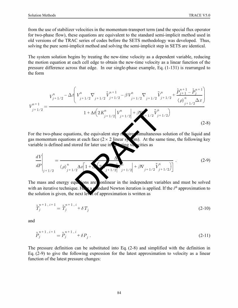
Solution Methods TRACE V5.0
from the use of stabilizer velocities in the momentum-transport term (and the special flux operatorfor two-phase flow), these equations are equivalent to the standard semi-implicit method used inold versions of the TRAC series of codes before the SETS methodology was developed. Thus,solving the pure semi-implicit method and solving the semi-implicit step in SETS are identical.
The system solution begins by treating the new-time velocity as a dependent variable, reducingthe motion equation at each cell edge to obtain the new-time velocity as a linear function of thepressure difference across that edge. In our single-phase example, Eq. (1-131) is rearranged tothe form
(2-8)
For the two-phase equations, the equivalent step requires simultaneous solution of the liquid andgas momentum equations at each face (2 × 2 linear system). At the same time, the following keyvariable is defined and stored for later use in updating velocities as
. (2-9)
The mass and energy equations are nonlinear in the independent variables and must be solvedwith an iterative technique. Here a standard Newton iteration is applied. If the ith approximation tothe solution is given, the next level of approximation is written as
(2-10)
and
. (2-11)
The pressure definition can be substituted into Eq. (2-8) and simplified with the definition inEq. (2-9) to give the following expression for the latest approximation to velocity as a linearfunction of the latest pressure changes:
Vj 1 2⁄+n 1+
Vj 1 2⁄+n ∆t V
j 1 2⁄+n ∇
j 1 2⁄+V
j 1 2⁄+n 1+ βV
j 1 2⁄+n ∇
j 1 2⁄+V
j 1 2⁄+n
– Pj 1+n 1+
Pjn 1+
–
ρ⟨ ⟩j 1 2⁄+n ∆x
---------------------------------+⎝ ⎠⎜ ⎟⎜ ⎟⎛ ⎞
–
1 t 2Kj 1 2⁄+n V
j 1 2⁄+n β V
j 1 2⁄+n
j 1 2⁄+∇+⎝ ⎠
⎛ ⎞∆+--------------------------------------------------------------------------------------------------------------------------------------------------------------------------------------------------------=
Vd
Pd-------
j 1 2⁄+
t∆
ρ⟨ ⟩j 1 2⁄+n x 1 t 2K
j 1 2⁄+n V
j 1 2⁄+n β V
j 1 2⁄+n
j 1 2⁄+∇+⎝ ⎠
⎛ ⎞∆+∆--------------------------------------------------------------------------------------------------------------------------------------------------=
Tjn 1 i 1+,+
Tjn 1 i,+
δTj+=
Pjn 1 i 1+,+
Pjn 1 i,+
δPj+=
DRAFT
84

TRACE V5.0 Solution Methods FOOBAR1234
Solution M
ethods
. (2-12)
These expressions are applied to the semi-implicit mass and energy equations [see Chapter 1Eqs. (1-120) and (1-121)] through the direct substitutions
, (2-13)
, and (2-14)
. (2-15)
Use of the state relationships and and a first-order Taylor seriesexpansion produces the linearized mass equation
(2-16)
and the linearized energy equation
Vj 1 2⁄+
n 1 i 1+,+V
j 1 2⁄+
n 1 i,+ dVdP-------
j 1 2⁄+
δPj δPj 1+–( )+=
Pjn 1+
Pn 1 i,+
δPj+⇒
Tjn 1+
Tjn 1 i,+
δTj+⇒
Vj 1 2⁄+n 1+ V
j 1 2⁄+
n 1 i,+ dVdP-------
j 1 2⁄+
δPj δPj 1+–( )+⇒
ρ P T,( )[ ] e P T,( )[ ]
∂ρ∂T--------
j
n 1 i,+
δTj∂ρ∂P-------
j
n 1 i,+
δPj+⎝ ⎠⎜ ⎟⎛ ⎞
∆t-------------------------------------------------------------------------------
ρ⟨ ⟩j 1
2---+
n dVdP-------
j 1 2⁄+
δPj δPj 1+–( ) ρ⟨ ⟩j 1 2⁄–n dV
dP-------
j 1 2⁄–
δPj 1– δPj–( )–
∆x--------------------------------------------------------------------------------------------------------------------------------------------------------------------------+
ρjn 1 i,+ ρj
n–∆t
---------------------------–xj∂∂– ρnV
n 1 i,+
⎝ ⎠⎛ ⎞=
∂ρ∂T--------
j
n 1 i,+
ejn 1 i,+
ρj˜ n 1 i,+ ∂e
∂T--------
j
n 1 i,+
+⎝ ⎠⎜ ⎟⎛ ⎞
δTj
∆t------------------------------------------------------------------------------------------------------------
∂ρ∂P-------
j
n 1 i,+
ejn 1 i,+
ρjn 1 i,+ ∂e
∂P-------
j
n 1 i,+
+⎝ ⎠⎜ ⎟⎛ ⎞
δPj
∆t----------------------------------------------------------------------------------------------------------+
DRAFT
85

Solution Methods TRACE V5.0
(2-17)
For the particular block-reduction technique used to solve this system of linear equations, anauxiliary variable is defined as
. (2-18)
This results in a set of linear equations for each cell in the form
. (2-19)
The first row in the above linear system can be considered to be the linearized mass conservationequation and the second to be the linearized energy equation. At each cell, this system is solvedfor the pressure and temperature variations in the form
. (2-20)
At this point, the constants represent the linearized predictions of change in pressure andtemperature assuming no further velocity changes at the cell faces. The coefficients accountfor contributions due to velocity changes (driven by changes in the pressure gradient).
The solution of the basic equations is completed in two steps. First, for each block represented byEq. (2-20), the pressure equation is isolated and Eq. (2-18) is substituted to provide a set of 10equations in the form
+
ρe⟨ ⟩j 1 2⁄+n dV
dP-------
j 1 2⁄+
δPj δPj 1+–( ) ρe⟨ ⟩j 1 2⁄–n dV
dP-------
j 1 2⁄–
δPj 1– δPj–( )–
∆x-------------------------------------------------------------------------------------------------------------------------------------------------------------------------------------
+ Pjn 1 i,+
dVdP-------
j 1 2⁄+
δPj δPj 1+–( ) dVdP-------
j 1 2⁄–
δPj 1– δPj–( )–
∆x--------------------------------------------------------------------------------------------------------------------------------- δPj
Vj 1 2⁄+
n 1 i,+V
j 1 2⁄–
n 1 i,+–
x∆--------------------------------------------+
ρjn 1 i,+
ejn 1 i,+
ρe( )jn–⎝ ⎠
⎛ ⎞
t∆------------------------------------------------------------–
xj∂
∂– ρnenVn 1 i,+
⎝ ⎠⎛ ⎞ Pj
n 1 i,+ Vj 1 2⁄+
n 1 i,+V
j 1 2⁄–
n 1 i,+–
x∆--------------------------------------------–=
P∆j 1 2⁄+
δPj 1+ δPj–=
aj 1 1, ,
aj 1 2, ,
aj 2 1, ,
aj 2 2, ,⎝ ⎠
⎜ ⎟⎜ ⎟⎜ ⎟⎛ ⎞
δPj
δTj⎝ ⎠⎜ ⎟⎛ ⎞ b
j 1,
bj 2,⎝ ⎠
⎜ ⎟⎜ ⎟⎜ ⎟⎛ ⎞ c
1j 1,
c1j 2,⎝ ⎠
⎜ ⎟⎜ ⎟⎜ ⎟⎛ ⎞
∆Pj 1 2⁄–
–crj 1,
crj 2,⎝ ⎠
⎜ ⎟⎜ ⎟⎜ ⎟⎛ ⎞
∆Pj 1 2⁄+
+=
δPj
δTi⎝ ⎠⎜ ⎟⎛ ⎞ b′
j 1,
b′j 2,⎝ ⎠
⎜ ⎟⎜ ⎟⎜ ⎟⎛ ⎞ c′
1j 1,
c′1j 2,⎝ ⎠
⎜ ⎟⎜ ⎟⎜ ⎟⎛ ⎞
∆Pj 1 2⁄–
–c′
rj 1,
c′rj 2,⎝ ⎠
⎜ ⎟⎜ ⎟⎜ ⎟⎛ ⎞
∆Pj 1 2⁄+
+=
b′c′
DRAFT
86
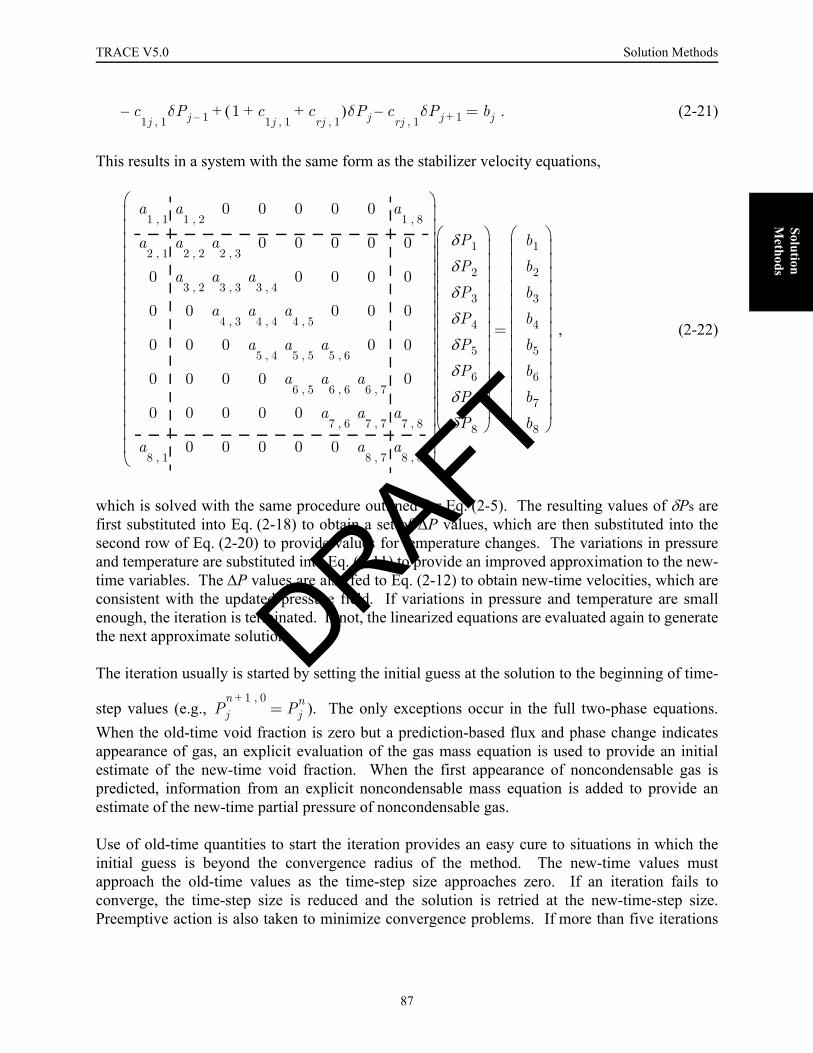
TRACE V5.0 Solution Methods FOOBAR1234
Solution M
ethods
. (2-21)
This results in a system with the same form as the stabilizer velocity equations,
, (2-22)
which is solved with the same procedure outlined for Eq. (2-5). The resulting values of δPs arefirst substituted into Eq. (2-18) to obtain a set of ∆P values, which are then substituted into thesecond row of Eq. (2-20) to provide values for temperature changes. The variations in pressureand temperature are substituted into Eq. (2-11) to provide an improved approximation to the new-time variables. The ∆P values are also fed to Eq. (2-12) to obtain new-time velocities, which areconsistent with the updated pressure field. If variations in pressure and temperature are smallenough, the iteration is terminated. If not, the linearized equations are evaluated again to generatethe next approximate solution.
The iteration usually is started by setting the initial guess at the solution to the beginning of time-
step values (e.g., ). The only exceptions occur in the full two-phase equations.When the old-time void fraction is zero but a prediction-based flux and phase change indicatesappearance of gas, an explicit evaluation of the gas mass equation is used to provide an initialestimate of the new-time void fraction. When the first appearance of noncondensable gas ispredicted, information from an explicit noncondensable mass equation is added to provide anestimate of the new-time partial pressure of noncondensable gas.
Use of old-time quantities to start the iteration provides an easy cure to situations in which theinitial guess is beyond the convergence radius of the method. The new-time values mustapproach the old-time values as the time-step size approaches zero. If an iteration fails toconverge, the time-step size is reduced and the solution is retried at the new-time-step size.Preemptive action is also taken to minimize convergence problems. If more than five iterations
c1j 1,
δPj 1–– 1 c1j 1,
crj 1,
+ +( )δPj crj 1,
δPj 1+–+ bj=
a1 1,
a1 2,
0 0 0 0 0 a1 8,
a2 1,
a2 2,
a2 3,
0 0 0 0 0
0 a3 2,
a3 3,
a3 4,
0 0 0 0
0 0 a4 3,
a4 4,
a4 5,
0 0 0
0 0 0 a5 4,
a5 5,
a5 6,
0 0
0 0 0 0 a6 5,
a6 6,
a6 7,
0
0 0 0 0 0 a7 6,
a7 7,
a7 8,
a8 1,
0 0 0 0 0 a8 7,
a8 8,⎝ ⎠
⎜ ⎟⎜ ⎟⎜ ⎟⎜ ⎟⎜ ⎟⎜ ⎟⎜ ⎟⎜ ⎟⎜ ⎟⎜ ⎟⎜ ⎟⎜ ⎟⎜ ⎟⎜ ⎟⎜ ⎟⎜ ⎟⎜ ⎟⎜ ⎟⎛ ⎞
δP1
δP2
δP3
δP4
δP5
δP6
δP7
δP8⎝ ⎠⎜ ⎟⎜ ⎟⎜ ⎟⎜ ⎟⎜ ⎟⎜ ⎟⎜ ⎟⎜ ⎟⎜ ⎟⎜ ⎟⎜ ⎟⎜ ⎟⎜ ⎟⎛ ⎞ b1
b2
b3
b4
b5
b6
b7
b8⎝ ⎠⎜ ⎟⎜ ⎟⎜ ⎟⎜ ⎟⎜ ⎟⎜ ⎟⎜ ⎟⎜ ⎟⎜ ⎟⎜ ⎟⎜ ⎟⎜ ⎟⎜ ⎟⎛ ⎞
=
Pjn 1 0,+
Pjn=
DRAFT
87

Solution Methods TRACE V5.0
are required to converge the solution on a given time step, the size of the next step is reduced bythe ratio of five divided by the last iteration count.
Solution of the SETS Stabilizer Mass and Energy Equations
The final step in the SETS method is the solution of the stabilizer mass and energy equations. Atthis point, the new-time velocities have been determined and can be treated as constants in thesolution of the equations. The equations vary from the mass and energy equations of the semi-implicit step only in that the densities and energies in flux terms are now evaluated at the newtime.
The mass and energy equations are linear in and respectively, with a structurethat is basically tridiagonal. For the loop flow problem, the general form of the mass equation canbe written as
, (2-23)
where superscripts representing new time have been dropped. This can be recognized asidentical in form to Eq. (2-5) and is solved with the same procedure.
The linear system produced by the stabilizer energy equation has the same coefficient matrix asthat of the mass equation. Time is saved by storing matrix factorization steps used in the massequation solution and by applying the results during the solution of the energy equation.
Final Solution for a New-Time Void Fraction
Solving the stabilizer mass and energy equations provides new-time values only for macroscopicdensities [ , , ] and macroscopic energy densities [ , ].
ρn 1+ ρe( )n 1+
a1 1,
a1 2,
0 0 0 0 0 a1 8,
a2 1,
a2 2,
a2 3,
0 0 0 0 0
0 a3 2,
a3 3,
a3 4,
0 0 0 0
0 0 a4 3,
a4 4,
a4 5,
0 0 0
0 0 0 a5 4,
a5 5,
a5 6,
0 0
0 0 0 0 a6 5,
a6 6,
a6 7,
0
0 0 0 0 0 a7 6,
a7 7,
a7 8,
a8 1,
0 0 0 0 0 a8 7,
a8 8,⎝ ⎠
⎜ ⎟⎜ ⎟⎜ ⎟⎜ ⎟⎜ ⎟⎜ ⎟⎜ ⎟⎜ ⎟⎜ ⎟⎜ ⎟⎜ ⎟⎜ ⎟⎜ ⎟⎜ ⎟⎜ ⎟⎜ ⎟⎜ ⎟⎜ ⎟⎛ ⎞
ρ1
ρ2
ρ3
ρ4
ρ5
ρ6
ρ7
ρ8⎝ ⎠⎜ ⎟⎜ ⎟⎜ ⎟⎜ ⎟⎜ ⎟⎜ ⎟⎜ ⎟⎜ ⎟⎜ ⎟⎜ ⎟⎜ ⎟⎜ ⎟⎜ ⎟⎛ ⎞ b1
b2
b3
b4
b5
b6
b7
b8⎝ ⎠⎜ ⎟⎜ ⎟⎜ ⎟⎜ ⎟⎜ ⎟⎜ ⎟⎜ ⎟⎜ ⎟⎜ ⎟⎜ ⎟⎜ ⎟⎜ ⎟⎜ ⎟⎛ ⎞
=
n 1+( )
αρg αρa 1 α–( )ρl αρgeg 1 α–( )ρlel
DRAFT
88
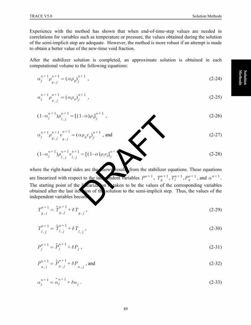
TRACE V5.0 Solution Methods FOOBAR1234
Solution M
ethods
Experience with the method has shown that when end-of-time-step values are needed incorrelations for variables such as temperature or pressure, the values obtained during the solutionof the semi-implicit step are adequate. However, the method is more robust if an attempt is madeto obtain a better value of the new-time void fraction.
After the stabilizer solution is completed, an approximate solution is obtained in eachcomputational volume to the following equations:
, (2-24)
, (2-25)
, (2-26)
, and (2-27)
. (2-28)
where the right-hand sides are the known results from the stabilizer equations. These equations
are linearized with respect to the independent variables , , , , and .The starting point of the linearization is taken to be the values of the corresponding variablesobtained after the last iteration of the solution to the semi-implicit step. Thus, the values of theindependent variables become
, (2-29)
, (2-30)
, (2-31)
, and (2-32)
. (2-33)
αjn 1+ ρ
g j,n 1+ αρg( )j
n 1+=
αjn 1+ ρ
a j,n 1+ αρa( )j
n 1+=
1 αjn 1+–( )ρ
l j,n 1+ 1 α–( )ρl[ ]j
n 1+=
αjn 1+ ρ
g j,n 1+ e
g j,
n 1+αρgeg( )j
n 1+=
1 αjn 1+–( )ρ
l j,n 1+ e
l j,n 1+ 1 α–( )ρlel[ ]j
n 1+=
Pn 1+ Tgn 1+ Tl
n 1+ Pan 1+ αn 1+
Tg j,n 1+ T
g j,n 1+ δT
g j,+=
Tl j,n 1+ T
l j,n 1+ δT
l j,+=
Pjn 1+ Pj
n 1+ δPj+=
Pa j,n 1+ Pa j,
n 1+ δPa j,
+=
αjn 1+ αj
n 1+δαj+=
DRAFT
89
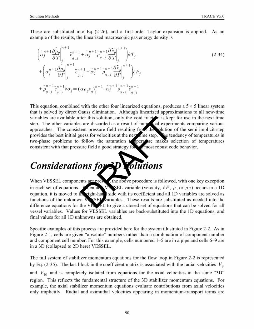
Solution Methods TRACE V5.0
These are substituted into Eq. (2-26), and a first-order Taylor expansion is applied. As anexample of the results, the linearized macroscopic gas energy density is
(2-34)
This equation, combined with the other four linearized equations, produces a 5 × 5 linear systemthat is solved by direct Gauss elimination. Although linearized approximations to all new-timevariables are available after this solution, only the void fraction is kept for use in the next timestep. The other variables are discarded as a result of numerical experiments comparing variousapproaches. The consistent pressure field resulting from the solution of the semi-implicit stepprovides the best initial guess for velocities at the next time step. The tendency of temperatures intwo-phase problems to follow the saturation temperature makes selection of temperaturesconsistent with that pressure field a good strategy for the most robust code behavior.
Considerations for 3D SolutionsWhen VESSEL components are present, the above procedure is followed, with one key exceptionin each set of equations. When any VESSEL variable (velocity, , , or ) occurs in a 1Dequation, it is moved to the right-hand side with its coefficient and all 1D variables are solved asfunctions of the unknown VESSEL variables. These results are substituted as needed into thedifference equations for the VESSEL to give a closed set of equations that can be solved for allvessel variables. Values for VESSEL variables are back-substituted into the 1D equations, andfinal values for all 1D unknowns are obtained.
Specific examples of this process are provided here for the system illustrated in Figure 2-2. As inFigure 2-1, cells are given “absolute” numbers rather than a combination of component numberand component cell number. For this example, cells numbered 1–5 are in a pipe and cells 6–9 arein a 3D (collapsed to 2D here) VESSEL.
The full system of stabilizer momentum equations for the flow loop in Figure 2-2 is representedby Eq. (2-35). The last block in the coefficient matrix is associated with the radial velocities
and and is completely isolated from equations for the axial velocities in the same “3D”region. This reflects the fundamental structure of the 3D stabilizer momentum equations. Forexample, the axial stabilizer momentum equations evaluate contributions from axial velocitiesonly implicitly. Radial and azimuthal velocities appearing in momentum-transport terms are
αjn 1+ ∂ρg
∂T---------
j
n 1+
eg j,n 1+ αj
n 1+ρg j,
n 1+ ∂eg∂T--------
j
n 1+
+⎝ ⎠⎜ ⎟⎛ ⎞
δTj
αjn 1+ ∂ρg
∂P---------
j
n 1+
eg j,n 1+ αj
n 1+ρg j,
n 1+ ∂eg∂P--------
j
n 1+
+⎝ ⎠⎜ ⎟⎛ ⎞
δPj
ρg j,n 1+
eg j,n 1+ δαj
+
+ αρgeg( )jn 1+ αj
n 1+– ρg j,
n 1+eg j,n 1+=
δP ρ ρe
V9
V10
DRAFT
90

TRACE V5.0 Solution Methods FOOBAR1234
Solution M
ethods
evaluated explicitly. This results in no coupling coefficients between velocity variables in theaxial momentum block and those in the radial (or azimuthal) blocks. In matrix notation, we have
. (2-35)
Solving the 1D portion of this system proceeds as before, isolating the 1D block as
Figure. 2-2. System for 3D solution examples.
1 2
3
4
5
7
8
6
91
2
5
3
4
6
8
9
10
7
a1 1,
a1 2,
0 0 0 0 0 a1 8,
0 0
a2 1,
a2 2,
a2 3,
0 0 0 0 0 0 0
0 a3 2,
a3 3,
a3 4,
0 0 0 0 0 0
0 0 a4 3,
a4 4,
a4 5,
0 0 0 0 0
0 0 0 a5 4,
a5 5,
a5 6,
0 0 0 0
0 0 0 0 a6 5,
a6 6,
a6 7,
0 0 0
0 0 0 0 0 a7 6,
a7 7,
a7 8,
0 0
a8 1,
0 0 0 0 0 a8 7,
a8 8,
0 0
0 0 0 0 0 0 0 0 a9 9,
a9 10,
0 0 0 0 0 0 0 0 a10 9,
a10 10,⎝ ⎠
⎜ ⎟⎜ ⎟⎜ ⎟⎜ ⎟⎜ ⎟⎜ ⎟⎜ ⎟⎜ ⎟⎜ ⎟⎜ ⎟⎜ ⎟⎜ ⎟⎜ ⎟⎜ ⎟⎜ ⎟⎜ ⎟⎜ ⎟⎜ ⎟⎜ ⎟⎜ ⎟⎜ ⎟⎜ ⎟⎜ ⎟⎛ ⎞
V1
V2
V3
V4
V5
V6
V7
V8
V9
V10⎝ ⎠⎜ ⎟⎜ ⎟⎜ ⎟⎜ ⎟⎜ ⎟⎜ ⎟⎜ ⎟⎜ ⎟⎜ ⎟⎜ ⎟⎜ ⎟⎜ ⎟⎜ ⎟⎜ ⎟⎜ ⎟⎜ ⎟⎜ ⎟⎛ ⎞ b1
b2
b3
b4
b5
b6
b7
b8
b9
b10⎝ ⎠⎜ ⎟⎜ ⎟⎜ ⎟⎜ ⎟⎜ ⎟⎜ ⎟⎜ ⎟⎜ ⎟⎜ ⎟⎜ ⎟⎜ ⎟⎜ ⎟⎜ ⎟⎜ ⎟⎜ ⎟⎜ ⎟⎜ ⎟⎛ ⎞
=
DRAFT
91
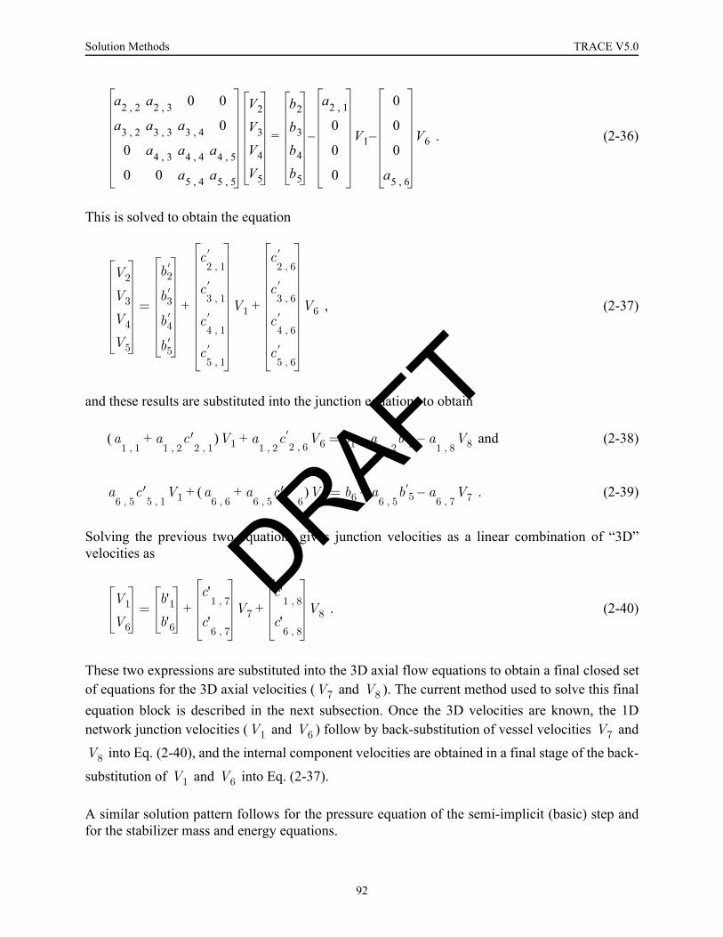
Solution Methods TRACE V5.0
. (2-36)
This is solved to obtain the equation
, (2-37)
and these results are substituted into the junction equations to obtain
and (2-38)
. (2-39)
Solving the previous two equations gives junction velocities as a linear combination of “3D”velocities as
. (2-40)
These two expressions are substituted into the 3D axial flow equations to obtain a final closed setof equations for the 3D axial velocities ( and ). The current method used to solve this finalequation block is described in the next subsection. Once the 3D velocities are known, the 1Dnetwork junction velocities ( and ) follow by back-substitution of vessel velocities and
into Eq. (2-40), and the internal component velocities are obtained in a final stage of the back-
substitution of and into Eq. (2-37).
A similar solution pattern follows for the pressure equation of the semi-implicit (basic) step andfor the stabilizer mass and energy equations.
a2 2, a2 3, 0 0
a3 2, a3 3, a3 4, 0
0 a4 3, a4 4, a4 5,
0 0 a5 4, a5 5,
V2
V3
V4
V5
b2
b3
b4
b5
a2 1,
0
0
0
– V1
0
0
0
a5 6,
– V6=
V2
V3
V4
V5
b2′
b3′
b4′
b5′
c2 1,′
c3 1,′
c4 1,′
c5 1,′
V1
c2 6,′
c3 6,′
c4 6,′
c5 6,′
V6+ +=
a1 1,
a1 2,
c′2 1,
+( )V1 a1 2,
+ c′2 6,
V6 b1 a1 2,
b′2– a1 8,
V8–=
a6 5,
c′5 1,
V1 a6 6,
a6 5,
c′5 6,
+( )V6+ b6 a6 5,
b′5–= a6 7,
V7–
V1
V6
b'1b'6
c'1 7,
c'6 7,
V7
c'1 8,
c'6 8,
V8+ +=
V7 V8
V1 V6 V7
V8
V1 V6
DRAFT
92

TRACE V5.0 Solution Methods FOOBAR1234
Solution M
ethods
The Capacitance Matrix MethodThe capacitance matrix method is applied in TRACE to provide an efficient numerical solutionalgorithm for solving the multidimensional vessel-matrix equations. Each vessel-matrix equationcombines the multidimensional mesh-cell or interface equations of all vessel components in themodeled system. The external or internal connectivity to the VESSEL component(s) of 1Dhydro-component loops introduces nonzero elements into the vessel matrix, coupling the vesselmesh cells or interfaces at the loop source connections to the vessel(s). The vessel-matrixequations that are solved are the semi-implicit pressure vessel-matrix equation in the outer-stagesolution and the stabilizer motion x- or r-, y- or , and z-direction vessel-matrix equations in theprepass stage of the solution and the stabilizer mass and energy vessel-matrix equations in thepostpass stage of the solution.
The capacitance matrix method is a direct L-U matrix-decomposition solution algorithm like thedirect full-matrix L-U matrix-decomposition solution algorithm used in TRAC-PF1/MOD1, but itdoes the L-U matrix decomposition on the banded portion of the vessel matrix with a moreefficient banded-matrix solver routine. The banded portion of the vessel matrix includes thenonzero coupling elements between a vessel mesh cell or interface and its six adjacent(neighboring) mesh cells or interfaces in 3D geometry. Nonzero elements outside the bandwidthof the matrix that couple vessel mesh cells or interfaces to nonadjacent mesh cells or interfaces ofthe same vessel or a different vessel component (due to 1D hydro-component loop connectivity)will be referred to as nonzero outlying elements. The effect that the nonzero outlying elementshave on the matrix-equation solution is accounted for in the capacitance matrix method by a directfull-matrix L-U matrix decomposition of a lower-order capacitance matrix. That solution is usedto modify the banded-matrix equation solution to give the desired solution of the vessel matrixwith its nonzero outlying elements. The capacitance matrix method was found in a study to bemore efficient than a direct full-matrix L-U matrix-decomposition solution of a vessel-matrixequation when fewer than 20% of the vessel-matrix rows have nonzero outlying elements. Formost system models (especially those with more than a hundred vessel mesh cells), only a fewpercent of the vessel-matrix rows have nonzero outlying elements. Thus, for a four-loop plantmodel with eight rows on nonzero outlying elements, the capacitance matrix method is faster thana full-matrix method by factors of 2, 4, 8, and 12 for vessel matrices of order 100, 200, 300, and400, respectively. Similar factors apply to computer memory storage for the vessel-matrixequation by the full-matrix method versus the capacitance matrix method.
We can summarize the above description of the method by noting that the capacitance matrixmethod is a direct two-stage procedure. In the first stage, the banded-matrix portion of the matrixequation is solved with an efficient banded-matrix solver to determine the solution for the vessel-matrix equation with zero-valued outlying elements. Then, if there are nonzero outlying elementsin the vessel matrix (1D hydro-component loops that connect back to a nonadjacent vessellocation generate nonzero outlying elements), the second stage evaluates a direct full-matrix L-Umatrix-decomposition solution of a much lower-order capacitance-matrix equation. Doing thisaccounts for the effect the nonzero outlying elements have on the vessel-matrix equation solution.This results in a modification of the banded-matrix solution to determine the solution of thevessel-matrix equation with nonzero outlying elements.
θ
DRAFT
93

Solution Methods TRACE V5.0
The following derivation determines the working equations and presents the four-step solutionprocedure programmed into the code. Given the vessel-matrix equation
A · x = b , (2-41)
where A is a known (vessel) matrix, x is an unknown (mass density, velocity, energy, or pressure)vector, and b is a known vector, let us partition A as follows into the sum of its banded matrix Band a matrix product E · R that has only the nonzero elements lying outside the bandwidth:
A · x = (B + E · R) · x = b . (2-42)
Consider the following example of how a simple form for A would appear when partitioned.
For A = , a matrix of order N, (2-43)
where r, s, t, and x are nonzero elements, N = 6 is the total number of rows and columns in A, andM = 2 is the number of rows in A having nonzero elements outside the three-diagonal bandwidth,then define
A = B + E · R (2-44)
where
B = , E =
x x O O O Ox x x O t OO x x x O OO O x x x Or O s x x xO O O O x x
N N×( )
x x O O O Ox x x O O OO x x x O OO O x x x OO O O x x xO O O O x x
O OO 1O OO O1 OO O
N N×( ) N M×( )
DRAFT
94

TRACE V5.0 Solution Methods FOOBAR1234
Solution M
ethods
R = , E · R = . (2-45)
(2-46)
Note that the nonzero elements in E are unity and in R are the actual nonzero outlying elements ofA. The term A is an N × N matrix with M rows having nonzero elements outside its bandwidth, Bis an N × N banded matrix, E is an N × M matrix, and R is an M × N matrix.
Multiply Eq. (2-42) by the inverse of the banded matrix, B to get
(I + B–1 · E · R) · x = B–1 · b . (2-47)
Define R · x = y and move its term in Eq. (2-47) to the right-hand side of the equation, giving
x = B–1 · b - B–1 E · y . (2-48)
Substitute Eq. (2-48) for x into Eq. (2-47) to give
(I + B–1 · E · R) · (B–1 · b - B–1 · E · y ) = B–1 · b . (2-49)
Expand Eq. (2-49), delete the B–1 · b term from both sides of the equation, and multiply theequation by (B–1 · E)–1 giving
(I + R · B–1 · E) · y = R · B–1 · b . (2-50)
Multiply Eq. (2-50) by the inverse of the matrix on its left-hand side to define y as follows:
y = (I + R · B–1 · E)–1 · R · B–1 · b . (2-51)
To determine x = A–1 · b, evaluate Eq. (2-51) for y and substitute y into Eq. (2-48) to evaluate x.
This evaluation procedure appears lengthy until we observe that it involves the following foursteps with some intermediate results used several times.
Step 1.Multiply the vector b and each of the M columns of E by the inverse of B.
= B–1 · b and = B–1 · E (2-52)
(N) (N x N) (N) (N x M) (N x N) (N x M)
r O s O O OO O O O t O
O O O O O OO O O O t OO O O O O OO O O O O Or O s O O OO O O O O O
M N×( ) N N×( )
x E
DRAFT
95

Solution Methods TRACE V5.0
Step 2.Multiply and from Step 1 by R.
= R · and = R · (2-53)
(M) (M x N) (N) (M x M) (M x N) (N x M)
Step 3.Evaluate Eq. (2-51) for y using and from Step 2.
y = ( I + )–1 · (2-54)
(M) (M x M) (M x M) (M)
Step 4.Evaluate Eq. (2-48) for the desired solution vector x using and from Step 1 and yfrom Step 3.
x = - · y (2-55)
(N) (N) (N x M) (M)
Computationally, Eq. (2-51) is solved by performing a single banded-matrix L-U matrixdecomposition to determine B-1. Then B-1 is applied to the 1+M column vectors of b and E by adirect forward-elimination and backward-substitution solution procedure. Equation (2-54)requires that a L-U matrix decomposition be applied to the full (nonbanded), but much smaller,
capacitance matrix I+ . The method becomes rapidly less efficient as the size of the capacitance
matrix I+ increases. The remainder of the computation involves matrix multiplications that areperformed efficiently on a vector computer.
Water PackingThe water-packing logic in the code is triggered under certain conditions (but not all conditions)when the code attempts during a time step to overfill (pack) a liquid-full finite-difference meshcell or to overextract (stretch) liquid from a liquid-full cell. The physical analog to water-packingevent is a water hammer; when cold water surges down a dead-end pipe filled with steam, a largepressure spike occurs when the last steam collapses and the water fills the pipe. This spike has avery short duration because of the low compressibility of liquid water, .
In any Eulerian finite-difference scheme, the boundary of a mesh cell behaves like the dead end ofa pipe in a water hammer event. This is especially true when condensation is present. Consider a
x E
b x R E
b R
R b
x E
x E
R
R DRAFT
96
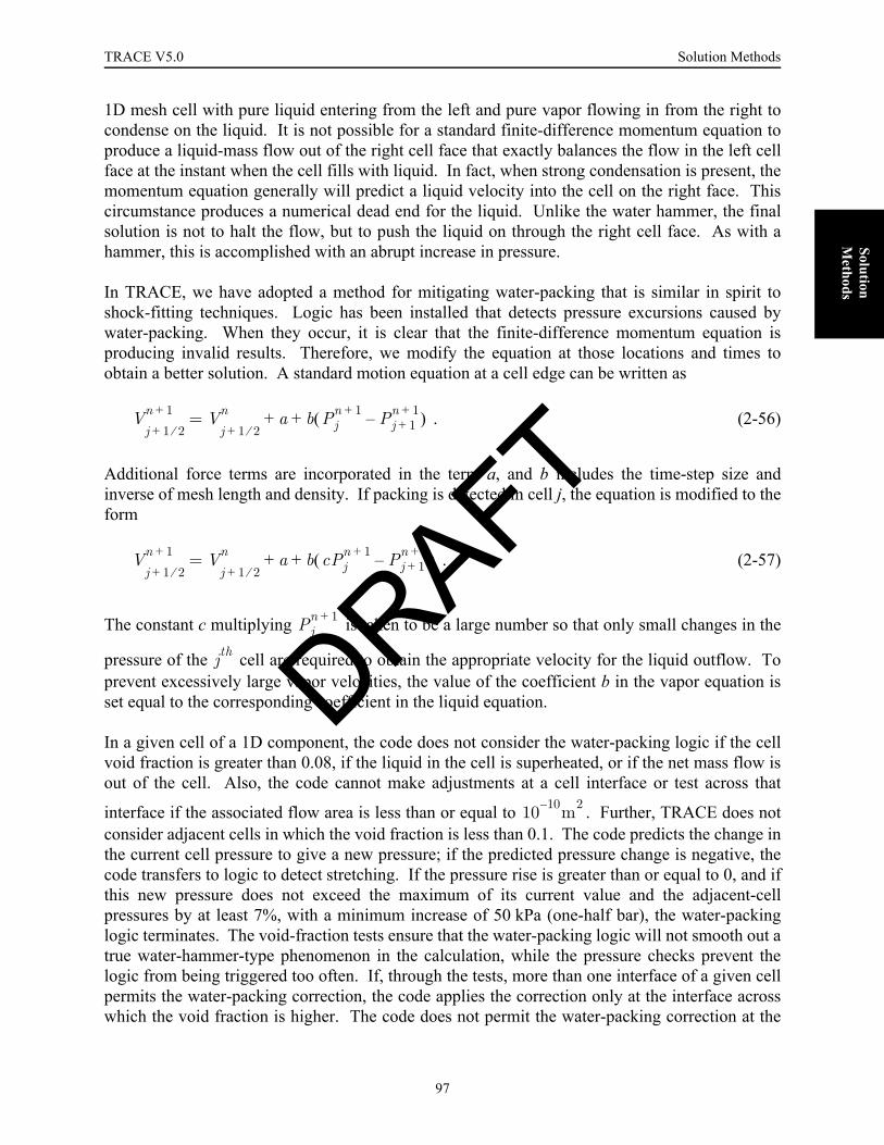
TRACE V5.0 Solution Methods FOOBAR1234
Solution M
ethods
1D mesh cell with pure liquid entering from the left and pure vapor flowing in from the right tocondense on the liquid. It is not possible for a standard finite-difference momentum equation toproduce a liquid-mass flow out of the right cell face that exactly balances the flow in the left cellface at the instant when the cell fills with liquid. In fact, when strong condensation is present, themomentum equation generally will predict a liquid velocity into the cell on the right face. Thiscircumstance produces a numerical dead end for the liquid. Unlike the water hammer, the finalsolution is not to halt the flow, but to push the liquid on through the right cell face. As with ahammer, this is accomplished with an abrupt increase in pressure.
In TRACE, we have adopted a method for mitigating water-packing that is similar in spirit toshock-fitting techniques. Logic has been installed that detects pressure excursions caused bywater-packing. When they occur, it is clear that the finite-difference momentum equation isproducing invalid results. Therefore, we modify the equation at those locations and times toobtain a better solution. A standard motion equation at a cell edge can be written as
. (2-56)
Additional force terms are incorporated in the term a, and b includes the time-step size andinverse of mesh length and density. If packing is detected in cell j, the equation is modified to theform
. (2-57)
The constant c multiplying is taken to be a large number so that only small changes in the
pressure of the cell are required to obtain the appropriate velocity for the liquid outflow. Toprevent excessively large vapor velocities, the value of the coefficient b in the vapor equation isset equal to the corresponding coefficient in the liquid equation.
In a given cell of a 1D component, the code does not consider the water-packing logic if the cellvoid fraction is greater than 0.08, if the liquid in the cell is superheated, or if the net mass flow isout of the cell. Also, the code cannot make adjustments at a cell interface or test across that
interface if the associated flow area is less than or equal to . Further, TRACE does notconsider adjacent cells in which the void fraction is less than 0.1. The code predicts the change inthe current cell pressure to give a new pressure; if the predicted pressure change is negative, thecode transfers to logic to detect stretching. If the pressure rise is greater than or equal to 0, and ifthis new pressure does not exceed the maximum of its current value and the adjacent-cellpressures by at least 7%, with a minimum increase of 50 kPa (one-half bar), the water-packinglogic terminates. The void-fraction tests ensure that the water-packing logic will not smooth out atrue water-hammer-type phenomenon in the calculation, while the pressure checks prevent thelogic from being triggered too often. If, through the tests, more than one interface of a given cellpermits the water-packing correction, the code applies the correction only at the interface acrosswhich the void fraction is higher. The code does not permit the water-packing correction at the
Vj 1 2⁄+n 1+ V
j 1 2⁄+n a b Pj
n 1+ Pj 1+n 1+–( )+ +=
Vj 1 2⁄+n 1+ V
j 1 2⁄+n a b cPj
n 1+ Pj 1+n 1+–( )+ +=
Pjn 1+
jth
10 10– m2
DRAFT
97
Solution Methods TRACE V5.0
interface opposite a FILL component if the velocities at both interfaces have the same sign or atthe interface at which the PUMP-component source is applied. Also, the code terminates thewater-packing logic for a given cell interface if choking is detected at that interface and if theinterface is either the first or last interface of a component.
The stretching logic is similar, although the code looks for a pressure drop in the current cell thatreduces its pressure to less than the minimum of 95% of its current value or 95% of theneighboring cells, with the additional constraint that the projected pressure must be less than thesaturation pressure corresponding to the current liquid temperature minus 20.0 K. The finalconstraint for stretching is that the test pressure cannot be below the lower pressure limit for theequation of state (see Chapter 11). For a stretch event, the code does not make an adjustment ata given interface if the void fraction on the other side of the interface is less than or equal to 0.1, ifthe liquid velocity at the interface is into the cell in which the stretch is detected, or if the PUMP-component source is applied at the interface.
The 3D VESSEL water-packing detection logic is very similar. The VESSEL, however, permitspacking to occur if the current cell void fraction is greater than 0.1, instead of the 0.08 in the 1Dcomponents. Also, in detecting a stretch, the code requires the pressure test to be 0.8 of that in the1D components.
DRAFT
98
TRACE V5.0 Heat Conduction Equations FOOBAR1234FOOBAR1234
Heat
Conduction
Equations
3 Heat Conduction Equations
FOOBAR1234FOOBAR1234FOOBAR1234
The nuclear reaction that takes place in the reactor core generates energy inside the fuel. In aPWR, that energy is then transferred to the primary fluid and crosses the steam-generator tubes tothe secondary fluid. In a BWR, that energy is deposited directly into the primary fluid, causingsteam to be generated, and ultimately driving the turbines. The code must calculate the heatconduction in the fuel and the steam-generator tubes to simulate correctly the heat-transferprocesses involved in thermal-energy transport. Also, the passive solid structures, such as pipingwalls, vessel walls, and the internal vessel structures, represent significant metal masses that canstore or release large amounts of thermal energy depending upon the reactor coolant temperature.Therefore, the code needs to model these additional structures. This chapter describes theunderlying theory employed by TRACE in order to model these phenomena.
NomenclatureThe following nomenclature applies to this chapter
= area in radial direction
= area in axial directionA = coefficient matrix
= nonzero elements of A
= equality vector
= elements of
= specific heat
C, D, E = nonzero submatrices of A
, = stability flags
HTC = heat transfer coefficient
= convective HTC
A
A∗
a
B
b B
cp
ft fss
h
DRAFT
99

Heat Conduction Equations TRACE V5.0
= gap conductance
= thermal conductivity
= number of nodes that segment the radial direction
= number of nodes that segment the axial direction
= heat flux vector
= heat generation rate per unit volume
= total heat flux
= radius
, = variables defined by Eqs. (3-26) and (3-27)
= radial coordinate
= time
= temperature
= temperature vector
= cell volume
= axial distance
= bottom of the fuel rod
= top of the fuel rod
= radial increment
= time increment
= slab thickness
= axial increment
= density
Subscripts = gas
= inner surface
= finite-difference indices
= liquid
= maximum
= outer surface
hgap
k
NR
NZ
q
q'''
qtotal
R
R+ R-
r
t
T
T
V
z
zb
zu
r∆
t∆
x∆
z∆
ρ
g
I
i j,
l
max
o
DRAFT
100

TRACE V5.0 Heat Conduction Equations FOOBAR1234FOOBAR1234
Heat
Conduction
Equations
= wall
Superscripts = axial direction
= current-time and new-time values
= predicted new-time values+, − = refers to material to the right and left of the interface, respectively
= new quantities when a fine mesh is added
Governing EquationsBecause the heat flux in a solid material is a vector quantity, the following general equationdescribes the heat-conduction process in an arbitrary geometry:
. (3-1)
In practice, the product is assumed to be constant for purposes of taking the time derivative.
The heat flux can be expressed in terms of the temperature gradient by Fourier’s law ofconduction (Ref. 3-1) as follows:
. (3-2)
Therefore, Eq. (3-1) becomes
. (3-3)
The thermal history of the reactor structure is obtained from a solution of the heat-conductionequation applied to different geometries. The next section discusses the coupling of the heat-conduction field equation in any of its many forms to the thermal-hydraulic field equationsrepresenting the fluid. Following this discussion, we present the details concerning the variousformulations of the heat-conduction equations that represent particular geometries typically foundin reactor systems. These geometries include cylindrical walls, slabs, and core fuel rods. Thefirst model analyzes heat conduction within the walls of the 1D loop components, such as pipewalls. The latter two are associated with heat transfer within structural components of the vessel.They are modeled similarly in the code, differing only in the area and volume calculations used inthe finite-difference equations.
w
j
n n 1+,
p
′
∂ ρcpT( )∂t
---------------------- ∇ q·+ q'''=
ρcp
q
q k∇T–=
ρcp∂T∂t-------- ∇ k∇T( ) q'''+·=
DRAFT
101
Heat Conduction Equations TRACE V5.0
Coupling of Thermal Hydraulics with the Reactor StructureThe energy transported by convective heat transfer from any structure into the different fluidphases is modeled using Newton’s law of cooling to represent the energy exchange rate betweenthe structure and the fluid phase. These terms appear in the energy equations of the different fluidphases. Chapter 6 discusses the logic used to determine which heat-transfer regime existsbetween the wall and fluid and which correlations for the wall heat-transfer coefficient (HTC) areused to represent the different regimes. The coupling algorithm (Figure 3-1) is currently implicitin terms of the wall temperature, liquid and vapor phase temperatures and explicit in terms of theheat transfer coefficient. For each new-time step, the wall HTCs ( ) of a given structure areevaluated using the surface wall temperatures ( ) and the fluid conditions obtained for the lasttime step. The new-time fluid-dynamics equations are solved using these HTCs, the new-timesurface temperatures, and the new-time fluid temperatures where the sum of the total energytransported into the fluid cell can be written as
. (3-4)
In general the finite volume approximation for the conduction equation (i.e. Eq. (3-3)) can bewritten as a set of linear equations for the new time heat structure temperatures:
A · = (3-5)
Given a convective heat transfer boundary condition, then the right-hand side vector B is afunction of the liquid and vapor phase temperatures for the fluid cell associated with the HS.Therefore, the derivative of Eq. (3-5) with respect to a change in the liquid phase temperature,yields:
A · = (3-6)
and the derivative of Eq. (3-5) with respect to a change in the vapor phase temperature, yields,
A · = (3-7)
The solution of Eq. (3-5) gives the predicted wall temperatures, in Eq. (3-4). The solution ofEq. (3-6) gives how the HS temperatures change given a change in the liquid phase temperatueand the solution of Eq. (3-7) gives how the HS temperatures change given a change in vapor
hTw
qtotaln 1+ hl
n Twp Tl
n–( ) hgn Tw
p Tgn–( )
hln ∂Tw
∂Tl----------- 1–⎝ ⎠
⎛ ⎞ hgn∂Tw∂Tl-----------+ Tl
n 1+ Tln–( ) hg
n ∂Tw∂Tg----------- 1–⎝ ⎠
⎛ ⎞ hln∂Tw∂Tg-----------+ Tg
n 1+ Tgn–( )
+
+
+=
T B
∂T∂Tl--------- ∂B
∂Tl---------
∂T∂Tg---------- ∂B
∂Tg----------
Twp
DRAFT
102

TRACE V5.0 Heat Conduction Equations FOOBAR1234FOOBAR1234
Heat
Conduction
Equations
phase temperatures. The solution of these three equations is the linearization of the conductionequation about the liquid and vapor phase temperatures.
. (3-8)
Notice that the coefficient matrix is not a function of the liquid or vapor phase temperatures,therefore, the difference between Eq. (3-5), Eq. (3-6), and Eq. (3-7) is the change in the right-hand side vector. The forward elimination developed for the solution of Eq. (3-5) is saved andused to obtain the linearization derivatives in Eq. (3-6) and Eq. (3-7). From the linearization of
the heat conduction equation, the two derivatives and are obtained for theradial HS node that is the wall of the HS. These two derivatives of how the HS wall temperaturechanges given a change in the liquid phase temperature and how the HS wall temperature changes
Figure. 3-1. Implicit coupling between hydrodynamics and structural heat transfer.
tn+1=tn+∆t
Calc. Material Properties(ρ,k,cp,...) and HTC (hl,hg)and Linearize ConductionEquation.
Solve the Fluid DynamicsEquations along with Linearized Conduction Eq.(αn+1,...,Tl
n+1,Tgn+1,Tw
n+1)
Calc. Wall Heat Fluxestn+1=tend
YES
PREPASS
OUTER
POSTPASS
NO
Tn 1+ Tn ∂T∂Tl--------- Tl
n 1+ Tln–( )
∂T∂Tg---------- Tg
n 1+ Tgn–( )+ +=
∂Tw ∂Tl⁄ ∂Tw ∂Tg⁄
DRAFT
103

Heat Conduction Equations TRACE V5.0
given a change in the vapor phase temperature together with Eq. (3-4) determines how the wallheat flux changes given a change in the liquid and vapor phase temperatures. This allows thefluid dynamics solution to be consistent with the linearized conduction equation.
Eq. (3-4) and Eq. (3-8) completely describe a single-side heat structure (i.e. a HS with convectiveheat transfer boundary condition on either the inside or outside surface of the heat structure). Forsingle-sided heat structures Eq. (3-5) through Eq. (3-7) are solved once and the linearizationcoefficients saved and used to update the HS temperature distribution each outer iteration (seeFigure 3-1).
For double-sided heat structures there are additional linearization terms associated with thechange in liquid and vapor phase temperatures on the other side of the heat structure.Experimentation with typical double-sided heat structures in a PWR and BWR power plant modelindicate that in most cases the derivative of the wall temperature given a change in the fluidtemperatures on the other side of the heat structure was small enough that it could be ignored.Therefore, for double-sided HS that derivatives of the phase temperatures on the other side of theheat structure are ignored in Eq. (3-4). However, for double-sided HS’s, Eq. (3-8) is not used toupdate the HS temperature distributions each outer iteration. For double-sided HS’s, Eq. (3-5)through Eq. (3-7) are solved for both the inner and outer surface. This ensures that for double-sided HSs the temperature distribution is consistent with the conduction equation and not anapproximate linearization of the conduction equation.
Figure. 3-2. Cylindrical wall geometry.
DRAFT
104

TRACE V5.0 Heat Conduction Equations FOOBAR1234FOOBAR1234
Heat
Conduction
Equations
Cylindrical Wall Heat ConductionThe temperature distribution within the walls of the 1D components is obtained from a finite-difference approximation to the 1D conduction equation,
. (3-9)
The finite-difference equations are derived by applying an integral method (Ref. 3-2) to the
elemental volumes shown in Figure 3-2. The general form of the volume ( ) is
(3-10)
where
. (3-11)
This formulation positions nodal points on material interfaces. Material properties are evaluated
between nodes. The boundary conditions applied to the inner ( ) and outer ( ) surfacesare
. (3-12)
For example, application of this boundary condition to the inner surface ( ) yields
ρcp∂T∂t-------- 1
r--- ∂
∂r------ rk∂T
∂r--------⎝ ⎠
⎛ ⎞ q'''+=
ith 1 i N< <
ri 1 2⁄–
ki 1 2⁄–
ri 1–∆--------------------------------Ti 1–
n 1+ri 1 2⁄–
ki 1 2⁄–
ri 1–∆--------------------------------
ri 1 2⁄+
ki 1 2⁄+
ri∆---------------------------------
12 t∆--------- ri ri 1–
ri 1–2∆4
--------------–∆⎝ ⎠⎜ ⎟⎛ ⎞
ρcp( )i 1 2⁄–
ri riri2∆
4--------+∆
⎝ ⎠⎜ ⎟⎛ ⎞
ρcp( )i 1 2⁄+
+⎭⎬⎫Ti
n 1+
ri 1 2⁄+
ki 1 2⁄+
ri∆---------------------------------Ti 1+
n 1+ 12--- ri ri 1–
r∆ i 1–2
4--------------–∆
⎝ ⎠⎜ ⎟⎛ ⎞
ρcp( )i 1 2⁄–
t∆---------------------------Ti
n q'''+⎩⎨⎧
–=
ri∆ri∆ri
2
4----------+
⎝ ⎠⎜ ⎟⎛ ⎞
ρcp( )i 1 2⁄+
∆t---------------------------Ti
n q'''+⎭⎬⎫
+
+
+
+
⎩⎪⎨⎪⎧
–
fin f tn ri,( )=
i 1= i N=
k∂T∂r--------
i 1 N,=
– hl Tl Ti–( ) hg Tg Ti–( )+[ ]±=
i 1=
DRAFT
105

Heat Conduction Equations TRACE V5.0
. (3-13)
The resulting linear equations are solved in a sequential fashion in the axial z-direction. For eachaxial position, a solution is achieved using Gaussian elimination.
A lumped-parameter solution is available to the user if the number of nodes is set equal to one.For this option the wall temperature is obtained from the equation,
. (3-14)
The subscripts and refer to the inner and outer radii, respectively.
Slab and Rod Heat ConductionStructures that can exchange heat with the fluid in a reactor vessel include downcomer walls andsupport plates, modeled as slabs, and vessel rods. These elements are referred to as heat-structurecomponents. Both nuclear and electrically heated rods or slabs can be analyzed. The effects ofgap conduction, metal-water reaction, and variable material properties are included (these modelsare documented in Chapter 8).
Only one rod within a cell may have hydro-cell coupling. This “average” rod is coupled to thefluid by Newton’s law of cooling. Any number of additional user-specified rods may be includedin each segment. The rod power factors (that is, relative to the average rod located within eachsegment) are specified by the user for these supplemental rods. The supplemental rods allow the
r3 2⁄
k3 2⁄
r1∆--------------------- 1
2--- r1∆r1
∆r12
4----------+
ρcp( )3 2⁄
t∆--------------------- r1 hl hg+( )+ +
⎩ ⎭⎨ ⎬⎧ ⎫
T1n 1+–
r3 2⁄
k3 2⁄
r1∆---------------------T2
n 1++
12--- r1 r1
r12∆
4--------+∆
⎝ ⎠⎜ ⎟⎛ ⎞
ρcp( )3 2⁄
t∆---------------------T1
n q'''+ r1 hlTln 1+ hgTg
n 1++––=
– r1 hlTln 1+ hgTg
n 1++[ ]
Tn 1+ 12--- 2 r r2∆
RI--------+∆
⎝ ⎠⎜ ⎟⎛ ⎞ ρcp
t∆--------Tn q'''+⎝ ⎠
⎛ ⎞ hlITlIn 1+
hgITgI
n 1+ 1 r∆RI------+⎝ ⎠
⎛ ⎞ hloTlon 1+ hgo
Tgo
n 1++[ ]+⎭⎬⎫
12--- 2 r r2∆
RI--------+∆
⎝ ⎠⎜ ⎟⎛ ⎞ ρcp
t∆--------⎝ ⎠
⎛ ⎞ hlI hgI1 r∆
RI------+⎝ ⎠
⎛ ⎞ hlo hgo+( )+ ++
⎩ ⎭⎨ ⎬⎧ ⎫
1–
+
+
+
⎩⎪⎨⎪⎧
=
I o DRAFT
106
TRACE V5.0 Heat Conduction Equations FOOBAR1234FOOBAR1234
Heat
Conduction
Equations
user to include hot rods in the reactor vessel. Such rods do not affect the fluid-dynamicscalculation because their contributions are already represented by average rods. They areincluded separately only for the purpose of determining their temperature response.
More than one slab may be located within a cell. Each slab is coupled to the fluid by Newton’slaw of cooling.
The user has four numerical calculation options for computing temperature distribution in slabsand rods. For thin slabs or rods of small diameter where the radial temperature profile is flat andaxial conduction is negligible, the user may choose the “lumped-parameter” solution. This optiongives the best calculational efficiency and should be used whenever it can be justified.
The second option is a 1D solution with implicit differencing in the radial direction and noconduction in the axial direction. This option is appropriate when steep axial profiles do not exist.
The third option is a 2D solution with implicit differencing in the radial direction and explicitdifferencing in the axial direction. This allows the very small radial node spacing required by thelarge radial power variations without severely limiting the time step. The explicit differencing inthe axial direction does limit the maximum time-step size for axial spacing. In many cases,however, this maximum time-step size is much greater than that used for the fluid-dynamicscalculation and is not restrictive. For those cases, the semi-implicit calculation gives goodcomputational efficiency.
The fourth option is the fully implicit, 2D finite-difference calculation. This is the best choice forcases where the axial temperature gradient is very large, such as in the vicinity of a quench front.Then the very fine axial noding that is required would cause the time step to be severely limited ifthe semi-implicit calculation was used. These methods are discussed in the following sections.
The Lumped-Parameter Solution.
The lumped-parameter equation for cylindrical coordinates is Eq. (3-14). If we choose and
for maximum stability, that equation reduces to
+
. (3-15)
ft 0=
fss 1=
Tn 1+ 12--- 2 r r2∆
RI--------+∆
⎝ ⎠⎜ ⎟⎛ ⎞ ρcp
t∆--------Tn q'''+⎝ ⎠
⎛ ⎞ hlITlIn 1+ hgI
TgI
n 1+++⎩⎨⎧
=
1 r∆RI------+⎝ ⎠
⎛ ⎞ hloTlon 1+ hgo
Tgo
n 1++[ ]⎭⎬⎫
12--- 2 r r2∆
RI--------+∆
⎝ ⎠⎜ ⎟⎛ ⎞ ρcp
t∆--------⎝ ⎠
⎛ ⎞ hlI hgI1 r∆
RI------+⎝ ⎠
⎛ ⎞ hlo hgo+( )+ ++
⎩ ⎭⎨ ⎬⎧ ⎫
1–
DRAFT
107

Heat Conduction Equations TRACE V5.0
For a solid rod, the axial temperatures are
. (3-16)
The lumped-parameter equation for the temperature of a slab is
, (3-17)
where is the slab thickness.
The Semi-Implicit Calculation.
Finite-difference equations are obtained by applying an integral method (Ref. 3-3) to appropriatedifferential volumes. The axial noding within a rod (see Figure 3-3) is typically the same or at afiner axial noding than the fluid component axial noding.
Consider a general differential volume (that is, the volume labeled in Figure 3-3). Usingexplicit differencing in the axial direction and implicit differencing in the radial direction, thefinite-difference equation for this volume is
(3-18)
Tn 1+ r∆2
------ρcp
t∆--------Tn q'''+ hloTlo
n 1+ hgoTgo
n 1++ +⎩ ⎭⎨ ⎬⎧ ⎫ rρcp∆
2 t∆--------------- hlo hgo
+ +⎩ ⎭⎨ ⎬⎧ ⎫
1–
=
Tn 1+
ρcp x∆t∆
---------------Tn q''' x∆+ hloTlon 1+ hgo
Tgo
n 1+ hlITlIn 1+ hgI
TgI
n 1++ + + +
ρcp x∆t∆
--------------- hlo hgohlI hgI
+ + + +-------------------------------------------------------------------------------------------------------------------------------------------------------=
∆x
i j,
ρcp( )ijTij
n 1+ Tijn–
t∆--------------------------- qij
'''–⎩ ⎭⎨ ⎬⎧ ⎫1
2--- ri ri
ri2∆
4--------+∆
⎝ ⎠⎜ ⎟⎛ ⎞
ri ri 1–ri 1–2∆4
--------------–∆⎝ ⎠⎜ ⎟⎛ ⎞
+zj z∆ j 1–+∆
2----------------------------
ri 1 2⁄+
ki 1 2 j,⁄+
Ti 1 j,+n 1+ Tij
n 1+–
ri∆-------------------------------------
⎝ ⎠⎜ ⎟⎜ ⎟⎛ ⎞
ri 1 2⁄–
ki 1 2 j,⁄–
Ti 1– j,n 1+ Tij
n 1+–
ri 1–∆-----------------------------------
⎝ ⎠⎜ ⎟⎜ ⎟⎛ ⎞
+
⎩ ⎭⎪ ⎪⎨ ⎬⎪ ⎪⎧ ⎫
zj zj 1–∆+∆2
---------------------------- ki j 1 2⁄+,
Ti j, 1+n Tij
n–
zj∆-------------------------------
⎝ ⎠⎜ ⎟⎜ ⎟⎛ ⎞
ki j 1 2⁄–,
Ti j, 1–n Tij
n–
zj 1–∆-------------------------------
⎝ ⎠⎜ ⎟⎜ ⎟⎛ ⎞
+
⎩ ⎭⎪ ⎪⎨ ⎬⎪ ⎪⎧ ⎫
+×
12--- ri ri
ri∆ 2
4----------+∆
⎝ ⎠⎜ ⎟⎛ ⎞
ri ri 1–ri 1–2∆4
--------------–∆⎝ ⎠⎜ ⎟⎛ ⎞
+×
=
DRAFT
108
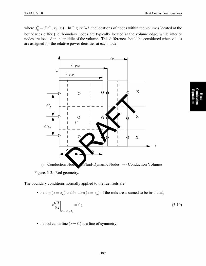
TRACE V5.0 Heat Conduction Equations FOOBAR1234FOOBAR1234
Heat
Conduction
Equations
where . In Figure 3-3, the locations of nodes within the volumes located at theboundaries differ (i.e. boundary nodes are typically located at the volume edge, while interiornodes are located in the middle of the volume. This difference should be considered when valuesare assigned for the relative power densities at each node.
The boundary conditions normally applied to the fuel rods are
• the top ( ) and bottom ( ) of the rods are assumed to be insulated,
; (3-19)
• the rod centerline ( ) is a line of symmetry,
Figure. 3-3. Rod geometry.
fijn f tn ri zj, ,( )=
r
z
X
X
X
O O O O O
O O O O O
O O O O O
O Conduction Nodes X Fluid-Dynamic Nodes ---- Conduction Volumes
∆ri-1 ∆ri
r-gap
r+gap
ro
i,j
∆zj
∆zj-1
z zu= z zb=
k∂T∂z--------
z zb zu,=
0=
r 0=
DRAFT
109

Heat Conduction Equations TRACE V5.0
; (3-20)
•heat transfer at the inner and outer gap surfaces and at the cladding
surface ( ) is specified using Newton’s law,
, and (3-21)
, (3-22)
where to conserve energy.
All properties (that is, , , and ) required by the difference equations are stored at the nodelocations. Linear interpolation is used to obtain properties between nodes (that is, at cellsurfaces). A node located at the interface between two dissimilar materials requires two sets ofproperties. Application of an integral technique to the differential volume in Figure 3-4 results inthe differential equation (after dividing through by the volume),
×
, (3-23)
where
∂T∂r--------
r 0=
0=
r rgap− rgap
+,=( )
r ro=
k∂T∂r--------
r rgap±=
hgap± T
rgap− T
rgap+–( )–=
k∂T∂r--------
r r0=
hfluid Tr0Tfluid–( )–=
hgap+ hgap
− rgap− rgap
+⁄( )=
ρ cp k
ρcp( )ijTij
n 1+ Tijn–
t∆---------------------------
⎝ ⎠⎜ ⎟⎛ ⎞
qij'''– r
i 1 2⁄+k
i 1 2 j,⁄+
Ti 1j+n 1+ Tij
n 1+–ri∆
----------------------------------⎝ ⎠⎜ ⎟⎛ ⎞
ri 1 2⁄–
ki 1 2 j,⁄–
+⎩⎨⎧
=
Ti 1 j,–n 1+ Tij
n 1+–
ri 1–∆-------------------------------------
⎝ ⎠⎜ ⎟⎜ ⎟⎛ ⎞
⎭⎪⎬⎪⎫ ri r∆ i
r∆ i2
4--------+
⎝ ⎠⎜ ⎟⎛ ⎞
ri r∆ i 1–r∆ i 1–2
4--------------+
⎝ ⎠⎜ ⎟⎛ ⎞
+
2-------------------------------------------------------------------------------------
1–
×
+ ki j 1 2⁄+,
Ti j, 1+n Tij
n–
zj∆-------------------------------
⎝ ⎠⎜ ⎟⎜ ⎟⎛ ⎞
ki j 1 2⁄–,
Ti j, 1–n Tij
n–
zj 1–∆-------------------------------
⎝ ⎠⎜ ⎟⎜ ⎟⎛ ⎞
+
⎩ ⎭⎪ ⎪⎨ ⎬⎪ ⎪⎧ ⎫
zj zj 1–∆+∆2
----------------------------1–
DRAFT
110

TRACE V5.0 Heat Conduction Equations FOOBAR1234FOOBAR1234
Heat
Conduction
Equations
(3-24)
and
. (3-25)
In the above equations,
(3-26)
and
. (3-27)
The superscripts "+" and "–" refer to the material to the right and left of the interface.
The semi-implicit finite-difference formulation for the slab is identical to that of the rod exceptfor the obvious geometric differences.
Figure. 3-4. Node located at the interface between two dissimilar materials.
ρcp( )ij
ρcp( )i+ j,
R+ ρcp( )+i− j,
R-
R+ R+−
-----------------------------------------------------------------------≡
ki j 1 2⁄+,
ki+ j 1 2⁄+,
R+ k+ i- j 1 2⁄+, R−
R+ R+−
[ ]--------------------------------------------------------------------------≡
R+ riri∆4
-------+⎝ ⎠⎛ ⎞ ri∆
2-------≡
R− riri 1–∆4
--------------–⎝ ⎠⎛ ⎞ ri 1–∆
2--------------≡
DRAFT
111
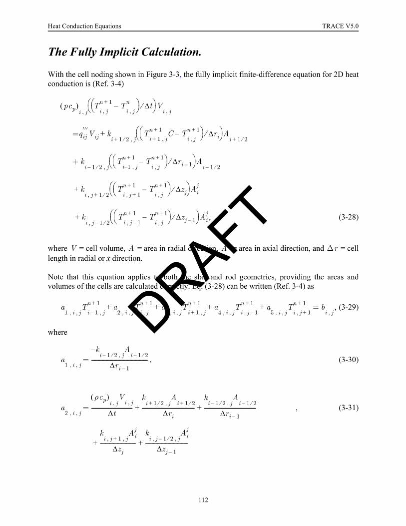
Heat Conduction Equations TRACE V5.0
The Fully Implicit Calculation.
With the cell noding shown in Figure 3-3, the fully implicit finite-difference equation for 2D heatconduction is (Ref. 3-4)
, (3-28)
where = cell volume, = area in radial direction, = area in axial direction, and = celllength in radial or x direction.
Note that this equation applies to both the slab and rod geometries, providing the areas andvolumes of the cells are calculated correctly. Eq. (3-28) can be written (Ref. 3-4) as
, (3-29)
where
, (3-30)
, (3-31)
pcp( )i j,
Ti j,n 1+ T
i j,n–⎝ ⎠
⎛ ⎞ t∆⁄⎝ ⎠⎛ ⎞ V
i j,
qij′′′Vij k
i 1 2 j,⁄+T
i 1 j,+n 1+ C T
i j,n 1+–⎝ ⎠
⎛ ⎞ ri∆⁄⎝ ⎠⎛ ⎞ A
i 1 2⁄++=
ki 1 2 j,⁄–
Ti 1– j,n 1+ T
i j,n 1+–⎝ ⎠
⎛ ⎞ ri 1–∆⁄⎝ ⎠⎛ ⎞ A
i 1 2⁄–+
ki j 1 2⁄+,
Ti j 1+,n 1+ T
i j,n 1+–⎝ ⎠
⎛ ⎞ zj∆⁄⎝ ⎠⎛ ⎞ Ai
j+
ki j 1 2⁄–,
Ti j 1–,n 1+ T
i j,n 1+–⎝ ⎠
⎛ ⎞ zj 1–∆⁄⎝ ⎠⎛ ⎞ Ai
j+
V A Aj ∆r
a1 i j, ,
Ti 1– j,n 1+ a
2 i j, ,T
i j,n 1+ a
3 i j, ,T
i 1+ j,n 1+ a
4 i j, ,T
i j 1–,n 1+ a
5 i j, ,T
i j 1+,n 1++ + + + b
i j,=
a1 i j, ,
ki 1 2 j,⁄–
Ai 1 2⁄–
–
ri 1–∆------------------------------------------=
a2 i j, ,
ρcp( )i j,
Vi j,
t∆-------------------------------
ki 1 2 j,⁄+
Ai 1 2⁄+
ri∆----------------------------------------
ki 1 2⁄ j,–
Ai 1 2⁄–
ri 1–∆---------------------------------------
ki j 1 j,+,
Aij
zj∆---------------------------
ki j 1 2 j,⁄–,
Aij
zj 1–∆--------------------------------
+ +
+ +
=
DRAFT
112

TRACE V5.0 Heat Conduction Equations FOOBAR1234FOOBAR1234
Heat
Conduction
Equations
, (3-32)
, (3-33)
, and (3-34)
. (3-35)
Eq. (3-29) is rewritten in matrix notation as
A · T = B (3-36)
or
, (3-37)
where
, (3-38)
a3 i j, ,
ki 1 2 j,⁄+
Ai 1 2⁄+
–
ri∆-------------------------------------------=
a4 i j, ,
ki j 1 2⁄–,
Aij
∆zj 1–---------------------------=
a5 i j, ,
ki j 1 2⁄+,
Aij–
zj∆-------------------------------=
bi j,
qi j,′′′
ρcp( )i j,
Ti j,n
t∆-------------------------------+
⎩ ⎭⎪ ⎪⎨ ⎬⎪ ⎪⎧ ⎫
Vi j,
=
D 1( ) E 1( )C 2( ) D 2( ) E 2( ) 0
C 3( ) D 3( ) E 3( )O
0C NZ 1–( ) D NZ 1–( ) E NZ 1–( )
C NZ( ) D NZ( )⎝ ⎠⎜ ⎟⎜ ⎟⎜ ⎟⎜ ⎟⎜ ⎟⎜ ⎟⎜ ⎟⎜ ⎟⎜ ⎟⎛ ⎞ T 1( )
T 2( )T 3( )M
M
T NZ 1–( )T NZ )( )⎝ ⎠
⎜ ⎟⎜ ⎟⎜ ⎟⎜ ⎟⎜ ⎟⎜ ⎟⎜ ⎟⎜ ⎟⎜ ⎟⎛ ⎞ B 1( )
B 2( )B 3( )M
M
B NZ 1–( )B NZ( )⎝ ⎠
⎜ ⎟⎜ ⎟⎜ ⎟⎜ ⎟⎜ ⎟⎜ ⎟⎜ ⎟⎜ ⎟⎜ ⎟⎛ ⎞
=
T j( )
T1 j,
T2 j,
M
TNR j,⎝ ⎠
⎜ ⎟⎜ ⎟⎜ ⎟⎜ ⎟⎜ ⎟⎜ ⎟⎜ ⎟⎛ ⎞
j 1 NZ,=( )= B j( )
b1 j,
b2 j,
M
bNR j,⎝ ⎠
⎜ ⎟⎜ ⎟⎜ ⎟⎜ ⎟⎜ ⎟⎜ ⎟⎜ ⎟⎛ ⎞
j 1 NZ,=( )=
DRAFT
113

Heat Conduction Equations TRACE V5.0
C(j) , (3-39)
D(j) , and (3-40)
E(j) . (3-41)
Matrix A is a symmetrical banded matrix. To solve for the temperatures, matrix A is inverted by amodified Cholesky method. Then the temperatures are computed from
T = A-1B . (3-42)
Note that Eq. (3-42) yields the predicted temperature distribution for the fully implicit 2D HS thatappears in Eq. (3-4). The linearization coefficients for the fully implicit 2D HS are:
= A-1 . (3-43)
= A-1 . (3-44)
a4 1 j, ,
0
a4 2 j, ,
O
0 a4 NR j,,⎝ ⎠
⎜ ⎟⎜ ⎟⎜ ⎟⎜ ⎟⎜ ⎟⎜ ⎟⎜ ⎟⎛ ⎞
j 2 NZ,=( )=
a2 1 j, ,
a3 1 j, ,
a1 2 j, ,
a2 2 j, ,
a3 2 j, ,
a1 3 j, ,
a2 3 j, ,
a3 3 j, ,
O
0 a1 NR j,,
a2 NR j,,⎝ ⎠
⎜ ⎟⎜ ⎟⎜ ⎟⎜ ⎟⎜ ⎟⎜ ⎟⎜ ⎟⎜ ⎟⎜ ⎟⎛ ⎞
j 1 NZ,=( )=
a5 1 j, ,
0
a5 2 j, ,
O
0 a5 NR j,,⎝ ⎠
⎜ ⎟⎜ ⎟⎜ ⎟⎜ ⎟⎜ ⎟⎜ ⎟⎜ ⎟⎛ ⎞
j 1 NZ 1–,=( )=
∂T∂Tl--------- ∂B
∂Tl---------
∂T∂Tg---------- ∂B
∂Tg----------
DRAFT
114

TRACE V5.0 Heat Conduction Equations FOOBAR1234FOOBAR1234
Heat
Conduction
Equations
Fine-Mesh Algorithm.
The reflood phase of a postulated LOCA is characterized by a sequence of heat-transfer and two-phase-flow regimes advancing rapidly through the vessel core. A correctly predicted thermalresponse from the fuel/heater rods during reflood requires a numerical technique that can modelthe quenching phenomena associated with the quench-front motion.
The leading edge of the quenching region is characterized by large variations of temperatures andheat fluxes within small axial distances ( ~ 1 mm) (Ref. 3-5). The front advancement iscontrolled by two heat-removal mechanisms, the first being axial conduction from the post-CHFregion ahead of the quenched region to the nucleate-boiling region behind the advancing film.The rod conduction model contains the necessary physics to analyze such phenomena. Thesecond is the precursory rod cooling associated with heat transfer to the slugs and dropletsentrained in the vapor field downstream of the quench front. The convective heat transferdiscussed in Chapter 6 contains the physics necessary to describe this phenomenon.
To model the inherently nonstationary, Lagrangian quench-front motion and to resolve the relatedthermal gradients, a fine-mesh rezoning technique (Ref. 3-6) is used during the refloodconduction calculations. The axial gradients encountered within the quenching region areresolved by the insertion of rows of transitory nodes (see Figure 3-5). These nodes are addedwhenever the surface temperature difference between adjacent nodes exceeds a heat transferregime dependent value ( ). If the heat transfer regime is film boiling, then isgiven by:
, (3-45)
If the heat transfer regime is transition boiling, then is given by:
, (3-46)
If the heat transfer regime is nucleate boiling, then is given by:
, (3-47)
For all other heat transfer regimes, is given by:
, (3-48)
∆z
∆Tmax ∆Tmax
∆Tmax Max 25 5 0.067∆Ts 0.000028 ∆Ts( )2+ +,⎝ ⎠⎛ ⎞=
∆Tmax
∆Tmax Min 25 5 0.067∆Ts+,( )=
∆Tmax
∆Tmax Min 5 25∆Ts-----------,
⎝ ⎠⎜ ⎟⎛ ⎞
=
∆Tmax
∆Tmax 25=
DRAFT
115
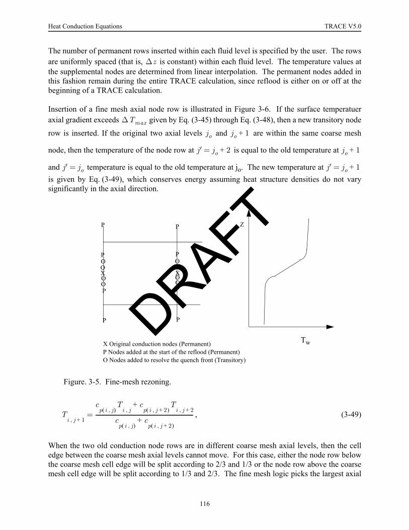
Heat Conduction Equations TRACE V5.0
The number of permanent rows inserted within each fluid level is specified by the user. The rowsare uniformly spaced (that is, is constant) within each fluid level. The temperature values atthe supplemental nodes are determined from linear interpolation. The permanent nodes added inthis fashion remain during the entire TRACE calculation, since reflood is either on or off at thebeginning of a TRACE calculation.
Insertion of a fine mesh axial node row is illustrated in Figure 3-6. If the surface temperatueraxial gradient exceeds given by Eq. (3-45) through Eq. (3-48), then a new transitory node
row is inserted. If the original two axial levels and are within the same coarse mesh
node, then the temperature of the node row at is equal to the old temperature at
and temperature is equal to the old temperature at jo. The new temperature at is given by Eq. (3-49), which conserves energy assuming heat structure densities do not varysignificantly in the axial direction.
, (3-49)
When the two old conduction node rows are in different coarse mesh axial levels, then the celledge between the coarse mesh axial levels cannot move. For this case, either the node row belowthe coarse mesh cell edge will be split according to 2/3 and 1/3 or the node row above the coarsemesh cell edge will be split according to 1/3 and 2/3. The fine mesh logic picks the largest axial
Figure. 3-5. Fine-mesh rezoning.
∆z
∆Tmax
jo jo 1+
j′ jo 2+= jo 1+
j′ jo= j′ jo 1+=
Tw
Z
X Original conduction nodes (Permanent)P Nodes added at the start of the reflood (Permanent)O Nodes added to resolve the quench front (Transitory)
X XO
O
O
OO O
OO
P
P
P
PP
P
P
P
Ti j 1+,
cp i j,( )
Ti j,
cp i j 2+,( )
Ti j 2+,
+
cp i j,( )
cp i j 2+,( )
+-------------------------------------------------------------------------=
DRAFT
116

TRACE V5.0 Heat Conduction Equations FOOBAR1234FOOBAR1234
Heat
Conduction
Equations
level of the two axial levels at the coarse mesh boundary to split into two axial node rows. Forthis case the new temperatures are based on the linear interpolation based on the original un-modified noding and temperatures. Since it is a single axial level that is split into two axial levels(i.e. one at 1/3 the height of the original axial level and the other at 2/3 the height of the originalaxial level), it is not necessary to do any averaging to ensure that energy is conserved with thenew noding.
When the axial surface temperature gradient between two node rows becomes less than one-halfof given by Eqs. (3-45) through (3-47), then two node rows are merged into one node
row. Inserting an axial node row based on and removing an axial node row based on
ensures that the fine mesh logic will not consistently insert and remove the sametransitory axial level every time step.
The above algorithm can analyze multiple quench fronts simultaneously. Both quenching anddryout are modeled automatically.
During the reflood phase, a number of surface conduction nodes are located within each fluid cell.Therefore, total heat transfer rate is obtained by summing the surface heat flux for each fine meshaxial level associated with a fluid cell.
(3-50)
It already has been noted that, for a given time step ( ), a minimum spacing ( ) betweenrows of conduction nodes exists because of the explicit axial differencing. For reflood
Figure. 3-6. Insertion of conduction nodes during reflood.
X X X X X X X X
X X X X X
X X X X
X X X Xj = jo
j = jo+1
j’ = jo+1
j’ = jo
j’ = jo+2
T(ri,zi)T’(ri,zi)
X Conduction Nodes---- Conduction Volume
∆Tmax
∆Tmax
∆Tmax( ) 2⁄
Q qj∂qj∂Tl--------- Tl
n 1+ Tln–( )
∂qj∂Tg---------- Tg
n 1+ Tgn–( )+ +⎝ ⎠
⎛ ⎞ Ajj∑=
∆t ∆z
DRAFT
117

Heat Conduction Equations TRACE V5.0
calculations, this axial spacing can be violated, resulting in stability problems. To avoid suchproblems, the time step is limited internally by a diffusion number. The user also can specifyminimum spacing ( ) beyond which supplemental rows of conduction nodes will not beadded. This additional advantage can prevent excessively large computer costs.
References3-1 G. B. Wallis, One Dimensional Two-Phase Flow (McGraw-Hill, Inc., New York, 1969).
3-2 Frank P. Incropera and David P. DeWitt, Fundamentals of Heat Transfer (John Wiley &Sons, New York, 1981).
3-3 P. J. Roache, Computational Fluid Dynamics (Hermosa Publishers, Albuquerque, NewMexico, 1972).
3-4 H. Akimoto, Y. Abe, and Y. Murao, “Implementation of an Implicit Method into HeatConduction Calculation of TRAC-PF1/MOD2 Code,” JAERI-memo 01-008 (February1989).
3-5 G. Yadigaroglu, “The Reflooding Phase of the LOCA in PWRs. Part I: Core Heat Transferand Fluid Flow,” Nuclear Safety 19 (1978).
3-6 Reactor Safety Research Program, “Quarterly Report for the Period July 1–September 30,1978,” Battelle Pacific Northwest Laboratories report PNL-2653-3 (NUREG/CR-0546)(1978).
∆zmin
DRAFT
118

FOOBAR1234FOOBAR1234FOOBAR1234
Drag M
odels
4 Drag Models
FOOBAR1234FOOBAR1234FOOBAR1234FOOBAR1234
As shown in Chapter 1, the liquid- and gas-field momentum equations each include terms for theinterfacial shear force and the wall drag force. Closure of these equations thus requires that wespecify the interfacial drag coefficient, , and the phasic wall drag coefficients, and ,for wall-liquid and wall-gas shear respectively. Typically, only one of the wall drag coefficientshas a non-zero value. For example, in either bubbly/slug or annular/mist flow, all of the wall dragis applied to the liquid phase and is set to zero. Both the models for the interfacial dragcoefficient and the wall drag coefficients are dependent upon the flow regime. These flow regimedependent closure models are discussed below, first for the interfacial drag and then for the walldrag.
NomenclatureThe following nomenclature applies to this chapter:
= minor radius of prolate ellipsoid
= flow area (m2)
= flow area of phase in stratified flow (m2)
= interfacial area per unit volume (m-1)
= projected area per unit volume (m-1)
= major radius of prolate ellipsoid
= particle drag coefficient
= Interfacial drag coefficient
= distribution parameter used in drift flux model
Ci Cwl Cwg
Cwg
a
A
Ak k
Ai″′
Ap″′
b
CD
Ci
C0
DRAFT
119

Drag Models TRACE V5.0
= wall drag coefficient for phase
= particle diameter, either bubble or drop, (m)
= pipe diameter (m)
= hydraulic diameter (m)
= entrainment fraction
= interfacial friction factor
= fraction of a cell that is quenched, i.e., in the pre-CHF flow regime
= wall friction factor for phase
= interfacial drag force per unit volume
= gravitational acceleration (m/s2)
= mass flux (kg/m2/s)
= height of liquid layer (m) in stratified flow
= volumetric flux (m/s)
= superficial velocity of phase (m/s)
= non-dimensional superficial velocity of phase
= Laplace no., equal to
= viscosity no. for phase ,
= pressure
= profile slip factor
= drop radius
= non-dimensional drop radius
= Reynolds no.
= perimeter of pipe in contact with gas phase in stratified flow
= width of gas-liquid interface in stratified flow
= temperature (K) of phase
= saturation temperature at the total pressure
Cwk k
d
D
Dh
E
fi
fQ
fwk k
Fi″′
g
G
hl
j
jk k
jk∗ k
La σ g ρ∆⁄( )1 2⁄
Nµk k Nµk µk ρkσσ
g ρ∆---------
1 2⁄⁄=
P
Ps
r
r*
Re
Sg
Si
Tk k
Tsat
DRAFT
120

TRACE V5.0 Drag Models FOOBAR1234FOOBAR1234FOOBAR1234
Drag M
odels
= weighted area-average value of the drift flux velocity
= velocity (m/s)
= void-weighted area average velocity for phase
= relative velocity (m/s)
= terminal velocity in infinite medium (m/s)
= non-dimensional terminal velocity
= Weber no.
= weighting factor
Greek = void fraction
= volume fraction of phase
= film thickness (m)
= non-dimensional gas film thickness defined by Eq. (4-116)
= density difference between liquid and gas phases (kg/m3)
= density (kg/m3)
= surface roughness
= liquid film flow rate per unit wetted perimeter (kg/s-m)
= viscosity (Ns/m2)
= dynamic viscosity (m/s2),
= non-dimensional gas velocities (see Eq. (4-54) and Eq. (4-56))
= pipe inclination angle (0 = horizontal)
= two-phase multiplier for phase flowing alone
= surface tension (N/m)
= shear stress (N/m2)
Subcripts = annular/mist flow regime
= bubble
= bubbly/slug flow regime
v gj
V
Vk k
Vr
V∞
V *∞
We
wf
α
αk k
δ
δ∗
ρ∆
ρ
ε
Γf
µ
ν ν µ ρ⁄=
π1π2
θ
φk2 k
σ
τ
AM
B
BS'
DRAFT
121

Drag Models TRACE V5.0
= core region in annular/mist flow
= critical value
= counter-current flow limit
= churn-turbulent bubbly flow
= Choe-Weisman (see Eq. (4-99))
= drop
= dispersed flow regime
= liquid film
= the liquid film or a value at a reference "film" temperature
= vapor-gas mixture
= interface
= inverted annular
= inverted slug
= Kataoka-Ishii drift flux model
= liquid
= laminar
= mixture value
= maximum value
= multi-particle
= non-stratified
= non-condensable gas
= nucleate boiling
= projected or particle
= value for film boiling or post-CHF regime
= value for normal pre-CHF regime
= relative
= value from Rayleigh-Taylor instability
= smooth
= value at saturated conditions
= value for laminar-smooth inverted annular regime
= stratified flow regime
c
crit
CCFL
CT'
C W–
d
DF
f
film
g
i
IA
IS
KI
l
lam
m
max
MP
ns
NC
NB
p
post CHF–
pre CHF–
r
R T–
s
sat
smooth
strat
DRAFT
122

TRACE V5.0 Drag Models FOOBAR1234FOOBAR1234FOOBAR1234
Drag M
odels
= Sauter mean value
= single-particle
= Taitel-Dukler (see Eq. (4-96))
= vapor
= volume median
= wall
= value for rough-wavy inverted annular regime
= in contact with liquid phase
= value from Kelvin-Helmholtz instability, that is, the Weber no. criterion.
= infinite medium or fully-developed
Interfacial DragThe two-phase flow model employed by TRACE is what is commonly referred to as the "sixequation" two-fluid model. This representation of the two-phase flow provides two characteristicvelocities in each coordinate direction. So, for example, for flow in a 1-D component, there aretwo velocities at every junction: one for the liquid phase, and another for the combined gas/vapormixture. The equations of motion for these two velocities are coupled by two interfacial terms:one resulting from the interfacial drag force between the phases and the other from themomentum transfer associated with mass transfer (see Chapter 1). It is the former, the interfacialdrag force arising from shear between the phases, that is the subject of this section.
The interfacial drag force per unit volume is given by
(4-1)
where is the interfacial drag force per unit volume, is the interfacial drag coefficient, and
is the relative velocity.
The interfacial drag coefficient is dependent upon the flow regime selected by the code. InTRACE, there are three distinct classes of flow regimes:
•Pre-CHF: these consist of the bubbly/slug and the annular/mist regimes as explained below in Bubbly/Slug Flow Regime and Annular/Mist Flow Regime.
•Stratified: the horizontal stratified flow regime is available for 1-D components that are either horizontal or inclined as explained in Stratified Flow Interfacial Drag Models.
•Post-CHF: this encompasses the "inverted" flow regimes that occur when the wall is too hot for liquid-wall contact, see Post-CHF Interfacial Drag Models .
SM
SP
T D–
v
vm
w
wavy
wet
We
∞
Fi″′ CiVr Vr=
Fi″′ Ci
Vr
DRAFT
123
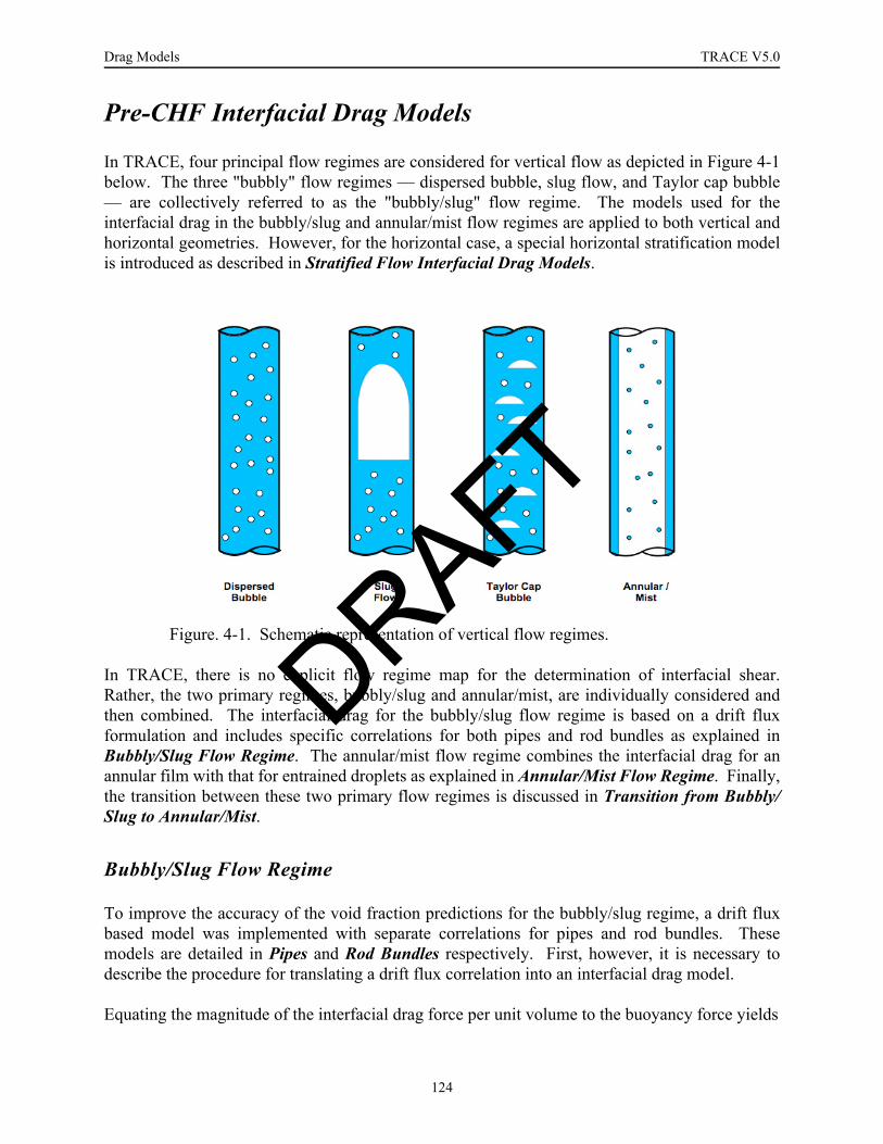
Drag Models TRACE V5.0
Pre-CHF Interfacial Drag Models
In TRACE, four principal flow regimes are considered for vertical flow as depicted in Figure 4-1below. The three "bubbly" flow regimes — dispersed bubble, slug flow, and Taylor cap bubble— are collectively referred to as the "bubbly/slug" flow regime. The models used for theinterfacial drag in the bubbly/slug and annular/mist flow regimes are applied to both vertical andhorizontal geometries. However, for the horizontal case, a special horizontal stratification modelis introduced as described in Stratified Flow Interfacial Drag Models.
In TRACE, there is no explicit flow regime map for the determination of interfacial shear.Rather, the two primary regimes, bubbly/slug and annular/mist, are individually considered andthen combined. The interfacial drag for the bubbly/slug flow regime is based on a drift fluxformulation and includes specific correlations for both pipes and rod bundles as explained inBubbly/Slug Flow Regime. The annular/mist flow regime combines the interfacial drag for anannular film with that for entrained droplets as explained in Annular/Mist Flow Regime. Finally,the transition between these two primary flow regimes is discussed in Transition from Bubbly/Slug to Annular/Mist.
Bubbly/Slug Flow Regime
To improve the accuracy of the void fraction predictions for the bubbly/slug regime, a drift fluxbased model was implemented with separate correlations for pipes and rod bundles. Thesemodels are detailed in Pipes and Rod Bundles respectively. First, however, it is necessary todescribe the procedure for translating a drift flux correlation into an interfacial drag model.
Equating the magnitude of the interfacial drag force per unit volume to the buoyancy force yields
Figure. 4-1. Schematic representation of vertical flow regimes.
DRAFT
124

TRACE V5.0 Drag Models FOOBAR1234FOOBAR1234FOOBAR1234
Drag M
odels
(4-2)
so that the interfacial drag coefficient becomes
(4-3)
To translate equation Eq. (4-3)[A-4] into a correlation for the interfacial drag coefficient, itremains to substitute for the relative velocity from the appropriate drift flux correlation. Then, theinterfacial drag coefficient, , will be a function of the weighted drift flux velocity, , and the
distribution parameter, .
To continue, a few definitions are necessary. A value averaged over the cross-sectional area isdenoted by the 's and defined by
(4-4)
where is any locally varying quantity and is the cross-sectional area. Of particular interestare the void-weighted area-averaged velocities, defined by
(4-5)
where the subscript indicates the phase ( for liquid and for the vapor/gas mixture). Thevoid-weighted area-averaged phase velocities are the velocities used in the field equations byTRACE. So, the relative velocity used by TRACE is then a "void-weighted area-averaged" valuegiven by
(4-6)
Next, the local drift velocity is given by
(4-7)
where is the volumetric flux and the weighted area-average value of the drift velocity, asdefined by Zuber and Findlay (Ref. 4-1), is then
(4-8)
α 1 α–( )g ρ∆ CiVr2=
Ciα 1 α–( )g ρ∆
Vr2
--------------------------------=
Ci v gj
C0
⟨ ⟩
X⟨ ⟩ 1A---- X Ad∫=
X A
VkαkVk⟨ ⟩αk⟨ ⟩
-------------------=
k l g
Vr Vg Vl–=
vgj Vg j–=
j
v gjαvgj⟨ ⟩
α⟨ ⟩-----------------=
DRAFT
125
Drag Models TRACE V5.0
Zuber and Findlay also introduced the distribution coefficient, , to account for phasedistribution effects, where
(4-9)
Next, the void-weighted area-averaged relative velocity, as used by TRACE, must be put in termsof these two drift flux parameters. Ishii and Mishima (Ref. 4-5) show that the area-averagedrelative velocity can be approximated by
(4-10)
where it is important to realize that
(4-11)
Rewrite equation [A-4] as
(4-12)
and substitute equation Eq. (4-10) to give
(4-13)
The last term on the right-hand-side of equation Eq. (4-13) will be denoted as the "profile slipfactor"
(4-14)
so equation Eq. (4-13) yields
(4-15)
for the interfacial drag coefficient.
C0
C0αj⟨ ⟩α⟨ ⟩ j⟨ ⟩
-----------------=
Vg Vl–⟨ ⟩v gj
1 α⟨ ⟩–------------------≈
Vg Vl–⟨ ⟩ Vg Vl–≠
Ciα 1 α–( )g ρ∆
Vg Vl–⟨ ⟩2--------------------------------
Vg Vl–⟨ ⟩2
Vr2
---------------------------·=
Ciα 1 α–( )3g ρ∆
v gj2
----------------------------------Vg Vl–⟨ ⟩2
Vr2
---------------------------·=
PsVg Vl–⟨ ⟩2
Vr2
---------------------------=
Ciα 1 α–( )3g ρ∆
v gj2
---------------------------------- Ps·=
DRAFT
126

TRACE V5.0 Drag Models FOOBAR1234FOOBAR1234FOOBAR1234
Drag M
odels
To evaluate the profile slip factor, it is necessary to relate the area-averaged relative velocity tothe void-weighted area-averaged phase velocities used by TRACE. Again from Ishii andMishima (Ref. 4-5), we have
(4-16)
so that the profile slip factor becomes
. (4-17)
The profile slip factor can be considerably less than unity and, for many situations, is much moreimportant in the calculation of the void fraction than is the drift flux velocity. For numericalreasons, its value is limited to be greater than 0.05.
To convert a drift flux model into an interfacial drag coefficient then requires the specification oftwo parameters: and . The drift flux velocity is specified uniquely for each of the bubbly/slug flow regimes as described below, whereas, one formulation is used for the distributioncoefficient for all of the bubbly/slug regimes (see Eq. (4-19)).
Pipes
For two-phase flow in pipes, two characteristic flow regimes are treated for the bubbly/slugregion. They are:
•Dispersed Bubbly Flow: bubbles are relatively small and may be spherical or distorted.
•Slug Flow or Taylor Cap Bubbly Flow: agglomeration has progressed to the extent that most of the gas phase is transported in large structures that are either slugs (for small diameter pipes) or Taylor cap bubbles (large diameter pipes).
For the dispersed bubbly flow regime, only one type of bubbly flow is considered: churn-turbulent flow. The churn-turbulent flow regime, according to Wallis (Ref. 4-2), represents atransition region between "ideal bubbly flow," in which bubbles rise uniformly and steadily, andslug flow in which large bubbles fill the tube and flow entirely in each other's wakes. The flowpattern is somewhat agitated and unsteady; agglomeration is important, and there is significantentrainment of bubbles in each other's wakes. The result is an increase in the relative velocitywith an increase in the number of bubbles present.
For the churn-turbulent regime, the correlation proposed by Ishii was selected (see Reference 4-3). The weighted drift flux velocity is given by
Vg Vl–⟨ ⟩1 C0 α⟨ ⟩–1 α⟨ ⟩–
-------------------------Vg C0Vl–=
Ps
1 C0 α⟨ ⟩–1 α⟨ ⟩–
-------------------------Vg C0Vl–⎝ ⎠⎜ ⎟⎛ ⎞
2
Vr2
-----------------------------------------------------------=
v gj C0
DRAFT
127
Drag Models TRACE V5.0
(4-18)
and the distribution parameter by
(4-19)
For small diameter pipes, the drift flux velocity given by Eq. (4-18) can exceed that for the slugflow regime (see Eq. (4-20)). To prevent this unrealistic situation, the churn-turbulent drift fluxvelocity is limited to always be less than that for slug flow.
As the void fraction increases, agglomeration becomes progressively more important and thebubbles grow to form either Taylor cap or slug bubbles. This regime will be referred to as the"cap/slug" regime in what follows. For this regime, Kataoka and Ishii (Ref. 4-4) developed onecorrelation with two parts to handle both the cases of cap bubble and slug flow. This model wasselected for the cap/slug regime in TRACE.
As presented by Kataoka and Ishii, the model has two formulations, one for low viscosity fluidsand another for high viscosity fluids. As the low viscosity formulation applies to fluids such aswater, it was implemented in TRACE. For relatively small diameter pipes, slug flow is possibleand the governing characteristic dimension becomes the pipe diameter. For this case, theweighted drift velocity is given by:
, for (4-20)
where the non-dimensional drift velocity is defined
, (4-21)
the non-dimensional hydraulic diameter is given by
, (4-22)
and the liquid viscosity number is
vgj 2σg ρ∆
ρl2
-------------⎝ ⎠⎜ ⎟⎛ ⎞ 1 4⁄
=
C0 1.2 0.2ρgρl-----–=
υgj+
0.0019 Dh*( )0.809 ρg
ρl-----
⎝ ⎠⎜ ⎟⎛ ⎞
0.157–
Nµl( )0.562–
= Dh* 30≤
υgj+ υgj
σg ρ∆
ρl2
-------------⎝ ⎠⎜ ⎟⎛ ⎞ 1 4⁄---------------------------=
Dh* =
Dh
σ g ρ∆⁄---------------------
DRAFT
128

TRACE V5.0 Drag Models FOOBAR1234FOOBAR1234FOOBAR1234
Drag M
odels
(4-23)
In relatively large diameter pipes, , slug bubbles cannot be sustained due to surfaceinstability, and they are disintegrated into cap bubbles. For this regime, Kataoka and Ishii gave
, for (4-24)
Eq. (4-20) and Eq. (4-24) are continuous with respect to pipe diameter and are programmed as
(4-25)
For both the cap bubble and slug formula, Kataoka and Ishii recommend using the samedistribution coefficient, , as for the churn-turbulent regime (see Eq. (4-19)).
It remains to specify how the transition between the dispersed bubble and the cap/slug bubbleregimes is handled. Air-water two-phase flow data indicate a clear transition for this transition inthe void fraction range from 20 to 30%. For values of the void fraction less than about 20%, theflow regime is dispersed bubble, and the data is well represented by the churn-turbulent model(Eq. (4-18) and Eq. (4-19)). As the void fraction increases, a transition to the Taylor cap bubbleregime occurs for void fractions greater than about 30% as represented by the Kataoka-Ishiimodel (Eq. (4-25) and Eq. (4-19)).
A simple linear ramp on the calculated drift flux velocity as a function of void fraction betweenthe limits of 20% to 30% provides a good fit to this transition region. The transition is theneffected by
(4-26)
where the linear ramp is
(4-27)
The implementation of this transition is illustrated in Figure 4-2 and Figure 4-3.
Nµlµl
ρl σ σ g ρ∆⁄⎝ ⎠⎛ ⎞
1 2⁄--------------------------------------------=
Dh* 30>
υgj+
0.030 ρgρl-----
⎝ ⎠⎜ ⎟⎛ ⎞
0.157–
Nµl( )0.562–
= Dh* 30≥
υgj+
0.0019 Min 30 Dh*,·
0.809 ρgρl-----
⎝ ⎠⎜ ⎟⎛ ⎞
0.157–
Nµl( )0.562–
=
C0
υgj wfCT υgj⎝ ⎠⎛ ⎞
CT1 wfCT–( ) υgj( )KI for 0.2 α 0.3≤ ≤·+·=
wfCT0.3 α–0.3 0.2–---------------------
⎝ ⎠⎜ ⎟⎛ ⎞
=
DRAFT
129
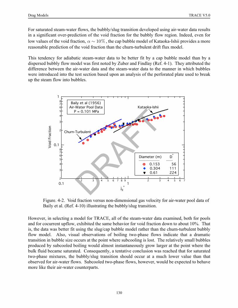
Drag Models TRACE V5.0
For saturated steam-water flows, the bubbly/slug transition developed using air-water data resultsin a significant over-prediction of the void fraction for the bubbly flow region. Indeed, even forlow values of the void fraction, , the cap bubble model of Kataoka-Ishii provides a morereasonable prediction of the void fraction than the churn-turbulent drift flux model.
This tendency for adiabatic steam-water data to be better fit by a cap bubble model than by adispersed bubbly flow model was first noted by Zuber and Findlay (Ref. 4-1). They attributed thedifference between the air-water data and the steam-water data to the manner in which bubbleswere introduced into the test section based upon an analysis of the perforated plate used to breakup the steam flow into bubbles.
However, in selecting a model for TRACE, all of the steam-water data examined, both for poolsand for cocurrent upflow, exhibited the same behavior for void fraction down to about 10%. Thatis, the data was better fit using the slug/cap bubble model rather than the churn-turbulent bubblyflow model. Also, visual observations of boiling two-phase flows indicate that a dramatictransition in bubble size occurs at the point where subcooling is lost. The relatively small bubblesproduced by subcooled boiling would almost instantaneously grow larger at the point where thebulk fluid became saturated. Consequently, a tentative conclusion was reached that for saturatedtwo-phase mixtures, the bubbly/slug transition should occur at a much lower value than thatobserved for air-water flows. Subcooled two-phase flows, however, would be expected to behavemore like their air-water counterparts.
Figure. 4-2. Void fraction versus non-dimensional gas velocity for air-water pool data of Baily et al. (Ref. 4-10) illustrating the bubbly/slug transition.
α 10%∼
!" #
# $ %#
DRAFT
130
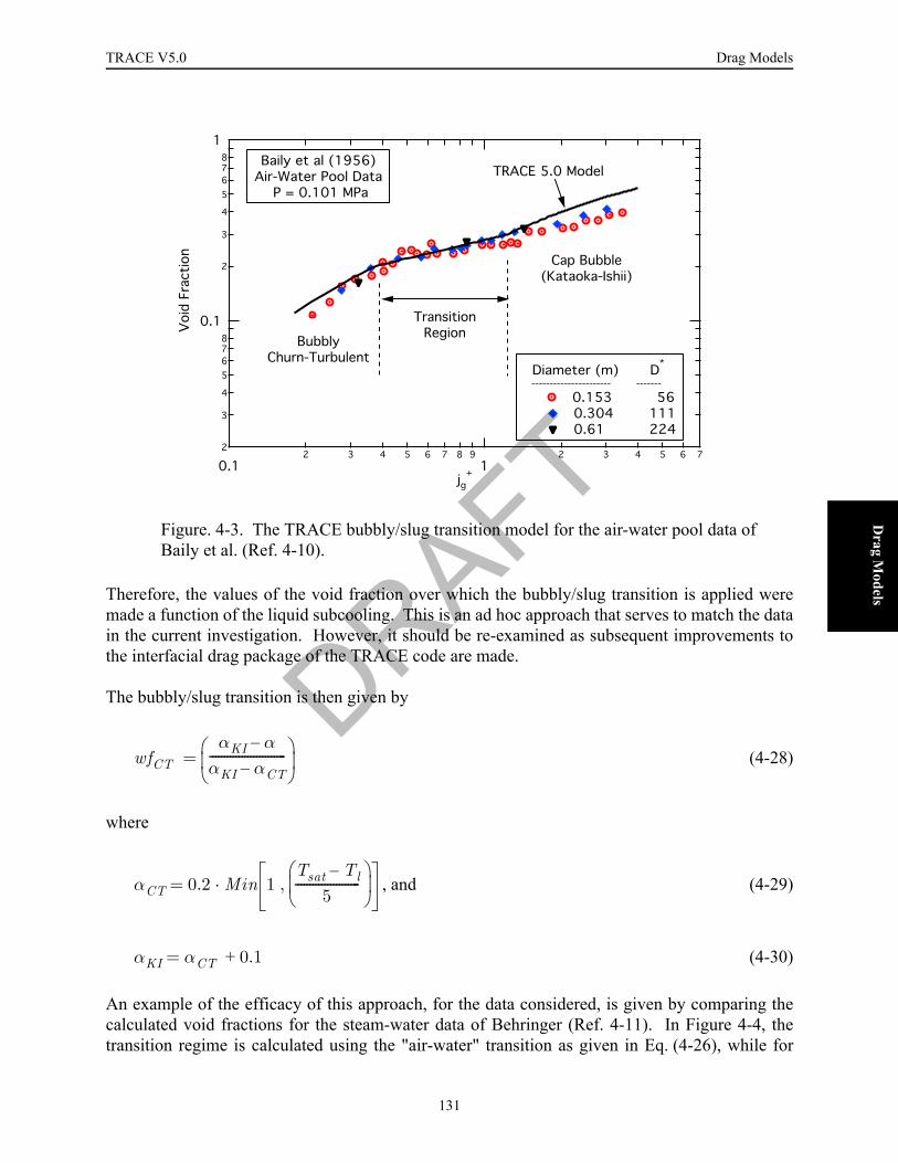
TRACE V5.0 Drag Models FOOBAR1234FOOBAR1234FOOBAR1234
Drag M
odels
Therefore, the values of the void fraction over which the bubbly/slug transition is applied weremade a function of the liquid subcooling. This is an ad hoc approach that serves to match the datain the current investigation. However, it should be re-examined as subsequent improvements tothe interfacial drag package of the TRACE code are made.The bubbly/slug transition is then given by
(4-28)
where
, and (4-29)
(4-30)
An example of the efficacy of this approach, for the data considered, is given by comparing thecalculated void fractions for the steam-water data of Behringer (Ref. 4-11). In Figure 4-4, thetransition regime is calculated using the "air-water" transition as given in Eq. (4-26), while for
Figure. 4-3. The TRACE bubbly/slug transition model for the air-water pool data of Baily et al. (Ref. 4-10).
!" #
# $ %#
!!"
!!#$!
&'!() %
wfCTαKI α–
αKI αCT–--------------------------
⎝ ⎠⎜ ⎟⎛ ⎞=
αCT 0.2 Min 1Tsat Tl–
5----------------------
⎝ ⎠⎜ ⎟⎛ ⎞
,·=
αKI αCT 0.1+=
DRAFT
131

Drag Models TRACE V5.0
Figure 4-5, the transition regime is calculated using the "steam-water" transition as given byEq. (4-29) and Eq. (4-30). The improvement is obvious as the "bump" present in Figure 4-5 hasnow disappeared.
Finally, for high flow rate conditions, turbulent shear stresses act to break up the bubbles therebyextending the dispersed bubbly regime to a much higher void fraction range. For such cases, theabove bubbly/slug transition would not be appropriate. However, the void fraction for high flowconditions is almost entirely determined by the distribution parameter, , and is unaffected bythe specification of the drift flux velocity. Therefore, no special treatment for high mass fluxconditions is needed.
Rod Bundles
The usage of pipe interfacial drag models for rod bundle geometries, as was done previously inTRAC-PF1/MOD2, resulted in core void fractions that were consistently over-predicted. Toimprove the accuracy of void fraction calculations, and hence core inventory, the Bestion (Ref. 4-6) drift flux model was implemented into TRACE. This model is used for the calculation of theinterfacial drag coefficient in the core region of the 3-D vessel component and for the 1-D CHANcomponent.
Figure. 4-4. Illustration of the problem with the air-water bubbly/slug transition model for the steam-water pool data of Behringer (Ref. 4-11).
!"!# "
!"!$!"!%&!"'!"&"%"!%&
(()* + , !"& !"
C0
DRAFT
132

TRACE V5.0 Drag Models FOOBAR1234FOOBAR1234FOOBAR1234
Drag M
odels
Based on previous experience, it was known that the Bestion model did a reasonably good job forlow-flow low-pressure conditions. Also, a study by Salay (Ref. 4-7) compared the predictivecapability of five drift flux models for high-pressure boil-off conditions and recommended theimplementation of the Bestion correlation in TRACE. This recommendation, in addition to thegood low-pressure performance of the Bestion model led to its adoption as the interfacial dragmodel for rod bundles.
The Bestion model is simply given by
(4-31)
and was originally specified with a constant distribution parameter, . In TRACE, it wasimplemented using the same distribution parameter as Ishii recommended for pipe flow. That is,
(4-32)
Figure. 4-5. Illustration of the improved bubbly/slug transition model for the steam-water pool data of Behringer (Ref. 4-11).
!"!# "
!"!$!"!%&!"'!"&"%"!%&
(()* + , ! !"
υgj 0.188 g ρDh ρg⁄∆=
C0 1.2=
C0 1.2 0.2ρgρl-----–=
DRAFT
133

Drag Models TRACE V5.0
At low pressure, these are essentially equivalent, and the dependence upon density ratio providesthe proper behavior as the pressure increases to the critical point.
However, assessment of TRACE for boiling water reactor conditions revealed a marked tendencyto under-predict the void fraction for values above about 40%. Consequently, the value of thedistribution parameter for rod bundles was set to unity, as recommended by Coddington andMacian (Ref. 4-12). With this change, the comparison with the FRIGG void fraction data (Ref. 4-13) is much improved, see Figure 4-6. Indeed, the average void fraction error was reduced from -5.0% to only 0.2%, and the RMS error was reduced from 6.0% to 2.7%.
Annular/Mist Flow Regime
The annular/mist flow regime in the TRACE code is treated as a superposition of interfacial dragon a liquid film and on entrained droplets. To complete this model, in addition to interfacial dragformulations for films and droplets, an entrainment model is needed to determine the fraction ofliquid flowing as droplets and a weighting scheme is needed to combine the individualcontributions. The following four sections describe each of these in turn.
Annular Film Models
Figure. 4-6. Comparison of calculated and measured values of the void fraction for the FRIGG experiments (Ref. 4-13) with the distribution parameter set to unity.
!"#$%
DRAFT
134

TRACE V5.0 Drag Models FOOBAR1234FOOBAR1234FOOBAR1234
Drag M
odels
For the annular flow regime, the interfacial drag force per unit volume for the liquid film is givenby
(4-33)
where is the interfacial friction factor and is the interfacial area per unit volume
for the liquid film. The interfacial friction coefficient from Eq. (4-1) is then defined as
(4-34)
The correlations used to evaluate the interfacial friction factor, , are detailed below. The
interfacial area per unit volume is computed from
(4-35)
which assumes that the volume fraction of the entrained droplets is much less than that of the gas/vapor mixture. That is,
(4-36)
which is a good approximation for annular/mist flow.
The TRAC-PF1/MOD2 model for the annular flow interfacial friction factor was that proposed byWallis (Ref. 4-8). Due to its general applicability, simple formulation and reasonably accuratepredictions, this model was retained in the TRACE code. However, for the special case ofcocurrent downflow, important for downflow tube condensation, the model of Wallis was foundto significantly over-predict the interfacial friction and hence under-predict the film thickness.Consequently, a modified form of the Asali-Hanratty correlation (Ref. 4-14) was implemented forthis regime.
The Wallis model (Ref. 4-8) treats the interfacial friction in annular flow as if the wavy filmrepresented an equivalent "sand roughness" for turbulent pipe flow. Thus, the friction factor wasgiven as a function of a dimensionless film thickness
(4-37)
and approximated by
F″′i film,
fi film,
A″′i film,
12---ρg Vr Vr·=
fi film,
A″′i film,
Ci film,
fi film,
A″′i film,
12---ρg·=
fi film,
A″′i film,
4Dh------- α=
α α αd+≈
fi film,
0.005 1 300 δD----+=
DRAFT
135
Drag Models TRACE V5.0
(4-38)
There are two principal assumptions built into this model:
•The flow is fully turbulent, i.e., , and
•The film surface is wavy, so that the wall roughness analogy applies.
These two assumptions are usually valid for vertical upflows but may not always be accurate fordownflow. As Wallis states, in horizontal or downflow at low gas velocities, the liquid film issmooth and the interfacial friction factor approaches the smooth pipe value.
Tube condensers are being proposed as safety equipment in the advanced passive reactor designs,so the TRACE code has been modified to enable accurate predictions of their heat removalcapacity. Both the wall and interfacial heat transfer coefficients in the annular flow regime usethe liquid film thickness as the characteristic length scale. So, to calculate pure-steamcondensation heat transfer with reasonable agreement, a good prediction of the film thickness isneeded. Therefore, an assessment of this capability was conducted for TRACE and led to twocode improvements:
•Wall Drag: an annular flow wall drag model was implemented (see the section titled Wall Drag below), and
• Interfacial Drag: a special correlation for cocurrent downflow (Asali and Hanratty, (Ref. 4-14)) was implemented.
The model of Asali and Hanratty for cocurrent downflow with entrainment was selected forTRACE, based on data comparisons with the downflow data of Andreussi and Zanelli (Ref. 4-15).The original form of the Asali and Hanratty correlation is
(4-39)
where is the smooth tube friction factor as a function of the gas Reynolds no. and the non-dimensional film thickness is
(4-40)
Note that the non-dimensional film thickness formula uses a friction velocity characterized by the
interfacial shear stress. This makes a function of the interfacial shear stress and hence of theinterfacial friction factor itself. That is, Eq. (4-39) is an implicit formulation and, as such, isunsuitable for implementation into the TRACE code as it would require an iterative solution.
fi film,
0.005 1 75 1 α–( )+=
fg 0.005≈
fifs--- 1– 0.45 Reg
0.2– δg+ 5.9–( )··=
fs
δg+ δ
τi ρg⁄νg
-------------------·=
δg+
DRAFT
136
TRACE V5.0 Drag Models FOOBAR1234FOOBAR1234FOOBAR1234
Drag M
odels
However, the definition of the interfacial shear stress
(4-41)
can be substituted into Eq. (4-40) so that, making use of the quadratic formula, Eq. (4-39) can besolved to yield an explicit formulation. This explicit formulation is given by
(4-42)
where the coefficients are
, and (4-43)
(4-44)
Note that the coefficient, , must be constrained to have a negative value.
Although not as accurate as the original implicit formulation, Eq. (4-42) still predicts thedownflow data of Andreussi and Zanelli well. Indeed, it is more accurate than any of the eightannular flow models tested except the original implicit formulation. For example, the averageRMS values for the relative error in the interfacial friction factor were -17.6% and 51.7%,respectively for the Wallis correlation but were reduced to -12.0% and 5.5% for the explicitformulation of the Asali-Hanratty model.
Entrainment Models
For the estimation of the interfacial drag coefficient in the annular/mist flow regime, as detailedin Annular/Mist Interfacial Drag Coefficient, it is necessary to know the fraction of the liquidflow that is composed of droplets. TRAC-PF1/Mod2 employed the Ishii-Mishima (Ref. 4-16)correlation to determine the mass fraction of liquid flowing as entrained droplets. Due to its largedatabase, reasonable accuracy and usage in other thermal-hydraulic codes such as RELAP5, thismodel has been retained in TRACE.
However, during the developmental assessment process, significant problems were observedwhen the Ishii-Mishima correlation was used outside the range of its database. Most specifically,one of the correlating variables that Ishii and Mishima used is the liquid film Reynolds no. The
τi fi12--- ρ· g Vr
2· ·=
fib – b2 4 c·–+
2----------------------------------------------
⎩ ⎭⎨ ⎬⎧ ⎫
2
=
b0.45 fs δ Vr· · ·
2 Reg0.2 νg· ·
---------------------------------------–=
c fs 1– 5.9 0.45
Reg0.2
-------------·+
⎝ ⎠⎜ ⎟⎜ ⎟⎛ ⎞
·=
c
DRAFT
137

Drag Models TRACE V5.0
correlation's database covers a film Reynolds no. range of , which is usuallyadequate for annular flow in small diameter pipes.
For large diameter pipes, such as the cold and hot legs of a PWR, the film Reynolds no. can be onthe order of 105 – 106. Consequently, the Ishii-Mishima correlation would be far outside therange of its database and significantly over-predict the entrainment fraction. Indeed, thecorrelation was found to predict nearly full entrainment at gas velocities below that necessary forthe initiation of entrainment. To remedy this problem, the Steen-Wallis entrainment correlationwas implemented for large diameter pipes while Ishii-Mishima was retained for geometries withsmall hydraulic diameters, such as steam generator tubes and rod bundles. Both of thesecorrelations are detailed below.
Ishii and Mishima developed a semi-empirical correlation for the fraction of the liquid fluxflowing as entrained drops. The theoretical basis came from a consideration of the roll waveentrainment mechanism. Using the entrainment inception criterion of Ishii and Grolmes (Ref. 4-17) as a starting point, they determined a critical film flow and assumed that all liquid flow inexcess of this critical value would be entrained. Refinements to this theory were then made toaccount for droplet deposition effects and to better match experimental data.
The entrained fraction was correlated as
(4-45)
where the subscript, , indicates the value for fully developed flow. In Eq. (4-45), the non-dimensional gas superficial velocity is defined by
, (4-46)
the non-dimensional tube diameter is scaled by the Taylor wavelength and given by
, (4-47)
and the film Reynolds no. is defined
(4-48)
370 Ref 6400< <
E∞ 7.25 7–×10 jg*( )2.5 D*( )1.25
Ref0.25tanh=
∞
jg∗ = jg
σ g ρ∆( )
ρg2 ρ ρg⁄∆( )
2 3⁄------------------------------------- 1 4⁄
--------------------------------------------------
D* Dh g ρ∆ σ⁄=
Ref1 α–( )ρlVlDh
µl------------------------------------=
DRAFT
138

TRACE V5.0 Drag Models FOOBAR1234FOOBAR1234FOOBAR1234
Drag M
odels
which is equivalent to the usual definition for film flow,
(4-49)
where is the film flow rate per unit wetted perimeter.
Finally, the non-dimensional gas flux and diameter were combined to define an effective Weberno. for entrainment,
(4-50)
yielding
(4-51)
Ishii and Mishima compared their correlation for the entrained fraction in fully developedannular/mist flow, given by Eq. (4-51), to an extensive set of experimental data in air-watersystems for the ranges:
Despite its semi-theoretical basis, the Ishii-Mishima correlation, as is the case for all empiricalformulations, should be used with caution outside the range of its database.
Furthermore, the behavior of the Ishii-Mishima correlation when extrapolated outside its databasewas considered to be unrealistic. Consequently, two changes were made to TRACE. First, thefilm Reynolds no. used in the Ishii-Mishima correlation was limited to the upper limit of thedatabase. That is,
(4-52)
1 < P < 4 (atm)
0.95 < D < 3.2 (cm)
370 < Ref < 6400
jg < 100 (m/s)
Ref4 Γf·µl
------------=
Γf
Wegρg jg
2 Dhσ
----------------------- ρ∆ρg------
⎝ ⎠⎜ ⎟⎛ ⎞
1 3⁄
=
E∞ 7.25 10×7–Weg
1.25Ref0.25tanh=
E∞ 7.25 10 7–× Weg1.25 Min 6400 Ref,
⎩ ⎭⎨ ⎬⎧ ⎫
0.25
·tanh=
DRAFT
139

Drag Models TRACE V5.0
Also, the Steen-Wallis entrainment correlation (Ref. 4-18) was implemented for usage in largediameter pipes. Here the definition of "large diameter" is simply taken to be the upper limit of thedatabase used by Ishii and Mishima, that is .
The Steen-Wallis correlation is a simple recasting of the formula presented by Paleev andFilippovich (Ref. 4-19) to better represent the property dependence upon liquid viscosity andexplicitly take into account the non-dimensional critical gas velocity introduced by Steen (Ref. 4-20). Paleev and Filippovich correlated the entrained fraction as
(4-53)
where the non-dimensional group, , is defined
(4-54)
and is the mean density of the gas-droplet flow.
In his comments on the paper of Paleev and Filippovich, Wallis (Ref. 4-18) states that theirproposed entrainment correlation [Eq. (4-53)] agrees substantially with the results obtained byWallis (Ref. 4-21) and Steen and Wallis (Refs. 4-20 and 4-22) as far as the effects of gas density,surface tension, and liquid density are concerned. However, their results were not in agreementwith the viscosity dependence reported by Steen who found that a change of a factor of 100 inliquid viscosity did not change the entrainment characteristics as long as the liquid flow rate washigh enough. Consequently, Wallis proposed modifying the correlation of Paleev and Filippovichto
(4-55)
where the non-dimensional gas velocity, , is that proposed by Steen to correlate the onset ofentrainment. Namely,
(4-56)
Steen found that the critical gas velocity for the onset of entrainment could be expressed by
(4-57)
However, Eq. (4-55) implies that the onset of entrainment begins at
Dh 3.2 (cm)>
E∞ 0.015 0.44 10 π1 104·[ ]log+=
π1
π1ρρl----
jg µlσ
----------⎝ ⎠⎜ ⎟⎛ ⎞ 2
=
ρ
E∞ 0.015 0.44log10 2.77 7×10 π· 22[ ]+=
π2
π2jgµgσ
----------ρgρl-----=
π2 crit,
2.46 4–×10∼
DRAFT
140

TRACE V5.0 Drag Models FOOBAR1234FOOBAR1234FOOBAR1234
Drag M
odels
(4-58)
Consequently, in TRACE, Eq. (4-55) has been rewritten as an explicit function of the critical non-dimensional gas velocity, :
(4-59)
and the inception criteria of Steen is used, (i.e., ).
Droplet Drag
The droplet drag force per unit volume is given by:
(4-60)
where is the drop drag coefficient, is the drop projected area per unit volume (m-1), and
is the drop relative velocity (m/s). Each of these quantities needed to compute the droplet
drag are described below.
First, the drop drag coefficient is taken from a correlation recommended by Ishii and Chawla(Ref. 4-23). The correlation is given by
(4-61)
and is an approximation to the drag curve for a solid sphere. In Eq. (4-61), the drop Reynolds no.is defined as a function of the relative velocity
(4-62)
where is the droplet Sauter mean diameter and the mixture viscosity is given by
(4-63)
π2 crit,
1.83 4–×10∼
π2 crit,
E∞ 0.015 0.44log10 0.9245π2
π2 crit,
-----------------⎝ ⎠⎜ ⎟⎛ ⎞ 2
·+=
π2 crit,
2.46 4–×10=
Fd″′ CDAd
″′ 12---ρgVr d,
2·=
CD Ad″′
Vr d,
CD24Red---------- 1 0.1Red
0.75+⎝ ⎠⎛ ⎞=
Redρg Vg Vd– dd
µm-----------------------------------------=
dd
µmµg
1 αd–( )2.5--------------------------=
DRAFT
141

Drag Models TRACE V5.0
Next, to compute the droplet projected area per unit volume, , it is necessary to obtain an
estimate of the fraction of the annular core occupied by the droplets, 1. From the definition ofthe entrained fraction, we have
(4-64)
where is the volume fraction of the annular core region (gas + drops), the product is
the drop volume fraction, and it has been assumed that, .
There is one unknown on the right-hand-side of Eq. (4-64) — the drop velocity, . BecauseTRACE employs a six-equation two-fluid model, the drop velocity is not directly calculated butmust be inferred. For the purpose of estimating the drop fraction, it is assumed that the dropletrelative velocity is small compared to the gas velocity, thus
(4-65)
and
(4-66)
The value of the droplet fraction calculated from Eq. (4-66) is then limited, so that
(4-67)
to protect against an unphysical result for a case where the gas velocity is low but the entrainmentfraction is non-zero.
From the definition of the Sauter mean diameter, the drop projected area per unit volume, is then
(4-68)
The next step is to determine the drop Sauter mean diameter that appears in the denominator ofEq. (4-68). In TRACE, this is accomplished through the evaluation of an empirical correlationbased on the local flow conditions and is calculated using the correlation of Kataoka, Ishii, andMishima (Ref. 4-24). They assumed that the mechanism for the generation of the droplets is that
1. Note that this droplet fraction is relative to the area of the annular core and not to the total cross-section. This terminology complicates the discussion but is retained here so that the model description will be consistent with the actual coding.
Ad′″
αd
αdE∞ 1 α–( ) Vl
αc Vd-------------------------------------
E∞ 1 α–( ) Vlα Vd
-------------------------------------≈=
αc αc αd
αc α≈
Vd
Vd Vg≈
αdE∞ 1 α–( ) Vl
α Vg-------------------------------------≈ E∞
jljg----=
αd E∞ 1 α–( )≤
Ad″′ 6
4---αc αd
dd--------------- 3
2---
α αd1 αd–( )dd
----------------------------= =
DRAFT
142
TRACE V5.0 Drag Models FOOBAR1234FOOBAR1234FOOBAR1234
Drag M
odels
of shearing from wave crests and proposed that the droplet diameter should be correlated as afunction of the film Reynolds no. in addition to the gas Reynolds no. and gas superficial velocity.The full form of their correlation is given by
(4-69)
where the gas Reynolds no. is defined
(4-70)
and the second subscript on the drop diameter, , indicates that the diameter is a volumemedian value. However, for the data used in developing this correlation, the film Reynolds no.
range only varied from 100 to 4700. This corresponds to a range in of 0.46 to 0.24.Consequently, they proposed a simplified form of the correlation where the dependency upon filmReynolds no. has been removed. The volume median diameter is then
, (4-71)
and it is this simplified form that is used in TRACE.
The droplet diameter used in TRACE for the calculation of both interfacial drag and heat transferis taken to be the Sauter mean diameter, that is, the drop diameter that has the same ratio ofinterfacial area to volume as that of the entire population. Kataoka et al. (Ref. 4-24) alsodeveloped an expression for the droplet size distribution. They fitted the data to the upper limitlog-normal distribution proposed by Mugele and Evans (Ref. 4-25). For the fitting parametersthat Kataoka et. al. used, the ratio of the Sauter mean to the volume median diameter is
(4-72)
Thus, Eq. (4-71) yields
(4-73)
dd vm,
0.028σ
ρg j2g
--------------⎝ ⎠⎜ ⎟⎛ ⎞
Ref1 6⁄–
Re2 3⁄g
µgµl-----
⎝ ⎠⎜ ⎟⎛ ⎞ 2 3⁄ ρg
ρl-----
⎝ ⎠⎜ ⎟⎛ ⎞ 1– 3⁄
=
Regρg jgDhµg
-------------------=
vm
Ref1 6⁄–
dd vm,
0.01
σρg j
2g
--------------⎝ ⎠⎜ ⎟⎛ ⎞
Re2 3⁄g
µgµl-----
⎝ ⎠⎜ ⎟⎛ ⎞ 2 3⁄ ρg
ρl-----
⎝ ⎠⎜ ⎟⎛ ⎞ 1– 3⁄
=
dd SM,
dd vm,
--------------- 0.796=
dd 0.008
σρg j
2g
--------------⎝ ⎠⎜ ⎟⎛ ⎞
Re2 3⁄g
µgµl-----
⎝ ⎠⎜ ⎟⎛ ⎞ 2 3⁄ ρg
ρl-----
⎝ ⎠⎜ ⎟⎛ ⎞ 1– 3⁄
=
DRAFT
143
Drag Models TRACE V5.0
for the Sauter mean diameter, where the subscript, , has been dropped.
Finally, the drop diameter calculated from Eq. (4-73) is limited to be in the range
. (4-74)
According to Cappiello (Ref. 4-26), this droplet diameter range was selected because it matchedthe range of the experimental data used in developing the correlation.
The final quantity in Eq. (4-60) left to be defined is the drop relative velocity, . As
explained below, the drop relative velocity is much less than the computed phasic velocitydifference. That is,
, (4-75)
because the computed liquid velocity represents both the film and the droplets. Consequently, thedrop terminal velocity is used to approximate the drop relative velocity.
The drop terminal velocity is taken from Ishii (Ref. 4-3). For spherical droplets in the Newtonregime, the relative velocity is given by:
(4-76)
For larger distorted drops, where the relative velocity is independent of the drop diameter, Ishiigives
. (4-77)
A criterion for the transition from the Newton to the distorted particle regime that is both simpleand physically meaningful is to simply limit the drop relative velocity given by Eq. (4-76) to beless than that for a distorted particle. The Newton regime would then be used for
(4-78)
Finally, the drop relative velocity estimated by either Eq. (4-76) or Eq. (4-77) is limited to be lessthan the value calculated for the phasic velocity difference by the solution of the two-fluidmomentum equations. That is,
SM
84 µm dd 4mm .≤ ≤
Vr d,
Vr d,
Vg Vl–
Vr d,
1.718 dd g ρ∆ρg
---------1 2⁄
1 αd–( )1.5
=
Vr d,
2 σg ρ∆ρg
2-------------
1 4⁄ 1 αd–( )
1.5=
dd 0.678 σg ρ∆---------≤
DRAFT
144

TRACE V5.0 Drag Models FOOBAR1234FOOBAR1234FOOBAR1234
Drag M
odels
. (4-79)
From Eq. (4-60), the interfacial drag force per unit volume on the drops is
(4-80)
or, in terms of the drop interfacial drag coefficient,
(4-81)
The drop interfacial drag coefficient, , is then defined by
(4-82)
Substituting for the drop projected area per unit volume, , from Eq. (4-68), the final form thedrop interfacial drag coefficient is
(4-83)
It remains to explain the procedure for superposing the interfacial drag forces for the drops andthe film. This is the subject of the following section.
Annular/Mist Interfacial Drag Coefficient
For the annular/mist flow regime, when the gas velocity is high enough, the liquid phase iscomprised of two distinct forms, the annular film and droplets carried in the gaseous core region.These two liquid forms interact with each other through the processes of entrainment and de-entrainment and have their own distinctly different characteristic velocity; indeed the droplets andthe liquid film can even flow counter-current to each other. Future versions of the TRACE codewill model each of these liquid forms with its own set of field equations thereby providingseparate velocities for the droplets and the annular film. However, in TRACE version 5.0, onlyone liquid field is available to model the combined droplet and annular film flows necessitating amodeling compromise.
Consequently, the drag forces between the gas-to-droplets and the gas-to-film are superposed. InTRAC-PF1/MOD1, this was done in the following simplified manner:
Vr d,
Vg Vl –≤
Fd″′ CDAd
″′ 12--- ρgVr d,
2·=
Fd″′ C
i drop,V
r d,2·=
Ci drop,
Ci drop,
CDAd″′ 1
2--- ρg·=
Ad″′
Ci drop,
CD ρg 3αcαd
4dd------------------· ·=
DRAFT
145

Drag Models TRACE V5.0
(4-84)
That is, the interfacial drag coefficients for the two liquid forms were simply added. The dragforce between the gas and the liquid was then
(4-85)
The result of this approach is that, as entrainment becomes significant, the drag force between thegas and liquid fields far exceeds that for the gas-to-film of annular flow. The calculated liquidfraction is then much too small and the calculated liquid velocity is much larger than isappropriate for a liquid film,
, (4-86)
which in turn causes the wall drag to be over-estimated.
To improve this situation, a significant modification was made to the model for the annular/mistflow regime in the development of the TRAC-PF1/Mod2 code. Here, the drag forces weresuperposed rather than just the coefficients. So,
(4-87)
and then
(4-88)
The evaluation of Eq. (4-88) requires that relative velocities for both the gas-drops and thegas-film be specified in addition to the drag coefficients. In Eq. (4-76) and Eq. (4-77), we haveseen how the drop terminal velocity, corrected for multi-particle effects, is used to estimate thegas-drop relative velocity. It remains to specify the relative velocity between the gas core and theannular film. In TRACE, it is assumed that
(4-89)
so Eq. (4-88) becomes
Ci AM,
Ci film,
C+i drop,
=
F″′i AM, C
i film,C+
i drop,⎝ ⎠⎛ ⎞ Vg Vl–( )
2=
Vf Vl Vd<
F″′i AM, C
i film,Vg Vf–( )
2C
i drop,Vg Vd–( )
2+=
Ci AM,
Ci film,
Vg Vf–( )2
C+i drop,
Vg Vd–( )2
Vg Vl–( )2
------------------------------------------------------------------------------------------------------=
Vg Vf– Vg Vl–≈
DRAFT
146

TRACE V5.0 Drag Models FOOBAR1234FOOBAR1234FOOBAR1234
Drag M
odels
(4-90)
This completes the description for the annular/mist flow regime, the following section describeshow the transition between the bubbly/slug and the annular/mist regimes is treated.
Transition from Bubbly/Slug to Annular/Mist
The replacement of the original TRAC-PF1/MOD2 interfacial drag model for the bubbly/slugregime with a drift flux based approach was done to:
• Improve accuracy of void fraction predictions, and
•Reduce void fraction oscillations at low-pressure conditions.
The improved accuracy is demonstrated during the developmental assessment, both for pipes andfor rod bundle geometries. Also, the root cause of the calculated void fraction oscillations wasdetermined to be the linear interpolation of the interfacial friction coefficient between the bubbly/slug and the annular/mist flow regimes that were used in TRAC-PF1/MOD2. This sectiondescribes the procedure adopted to resolve this oscillation problem.
The magnitude of the interfacial friction coefficient varies by orders of magnitude between thebubbly/slug and the annular/mist flow regime as illustrated below in Figure 4-7. In this figure, thebubbly/slug interfacial drag coefficient was calculated using the drift flux model for pipegeometry. It has a peak value in the void fraction range of 20% to 25%, as expected, and thendecreases dramatically as the annular flow regime is approached1.
Because of this large difference in magnitude of the interfacial friction coefficient for these tworegimes, a natural transition is provided by a simple power law weighting scheme. That is:
(4-91)
An example of this transition is provided in Figure 4-8 for these low-pressure low-flowconditions. The key point is that the flow regime transition is consistent with the interfacial dragmodels. Thus, the transition void fraction will change as the flow conditions change unlike thestatic transition of TRAC-PF1/MOD2. The result of the implementation of this power lawweighting flow regime transition in TRACE is the almost complete elimination of the voidfraction oscillation that was observed for low-pressure low-flow conditions.
1. The inflection that occurs in the bubbly/slug curve of Figure 4-7 at a void fraction of about 75% is due to the limitation on the profile slip factor, .
Ci AM,
Ci film,
C+i drop,
Vr d,
Vg Vl–( )2
-------------------------2
=
Ps 0.05≥
Ci C2i BS, Ci AM,
2+=
DRAFT
147
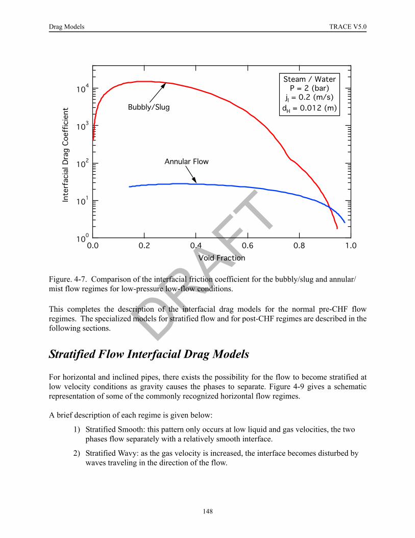
Drag Models TRACE V5.0
This completes the description of the interfacial drag models for the normal pre-CHF flowregimes. The specialized models for stratified flow and for post-CHF regimes are described in thefollowing sections.
Stratified Flow Interfacial Drag Models
For horizontal and inclined pipes, there exists the possibility for the flow to become stratified atlow velocity conditions as gravity causes the phases to separate. Figure 4-9 gives a schematicrepresentation of some of the commonly recognized horizontal flow regimes.
A brief description of each regime is given below:
1) Stratified Smooth: this pattern only occurs at low liquid and gas velocities, the two phases flow separately with a relatively smooth interface.
2) Stratified Wavy: as the gas velocity is increased, the interface becomes disturbed by waves traveling in the direction of the flow.
Figure. 4-7. Comparison of the interfacial friction coefficient for the bubbly/slug and annular/mist flow regimes for low-pressure low-flow conditions.
!
DRAFT
148

TRACE V5.0 Drag Models FOOBAR1234FOOBAR1234FOOBAR1234
Drag M
odels
3) Plug/Slug Flow: a further increase in the gas velocity causes the waves at the interface to bridge the channel and form a frothy slug that is propagated with a high velocity.
4) Annular/Dispersed: a still higher gas velocity results in the formation of a gas core with a liquid film around the periphery of the pipe. This regime is usually accompanied by the presence of entrained droplets due to the high gas velocity.
5) Dispersed Bubble: this flow pattern is similar to that of vertical flow; at low liquid velocities the gas bubbles tend to travel in the upper half of the pipe, whereas at high liquid velocities the bubbles are dispersed.
Not all of these horizontal flow regimes are explicitly considered by TRACE. The "dispersedbubble" and "annular/dispersed" regimes are treated by their vertical flow analogs, that is, by thebubbly/slug and annular/mist flow regimes described in Bubbly/Slug Flow Regime and Annular/Mist Flow Regime respectively. No special alterations to these regimes are made for differencesthat might occur in horizontal flow. The "stratified smooth" regime is explicitly considered asdescribed in Interfacial Friction for Stratified Flow. However, the other two regimes, "stratifiedwavy" and "plug/slug flow" are not explicitly considered but rather are treated as transitionregimes that occur as the flow regime is transitioning from stratified flow to a non-stratified flowpattern.
Figure. 4-8. Close-up of interfacial drag curve giving an example of the bubbly/slug to annular/mist transition using a power law weighting scheme.
!
"#$#
%# &'
& (&)
DRAFT
149
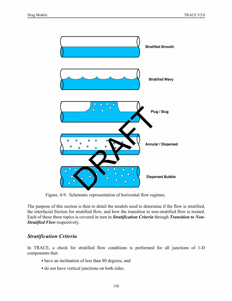
Drag Models TRACE V5.0
The purpose of this section is then to detail the models used to determine if the flow is stratified,the interfacial friction for stratified flow, and how the transition to non-stratified flow is treated.Each of these three topics is covered in turn in Stratification Criteria through Transition to Non-Stratified Flow respectively.
Stratification Criteria
In TRACE, a check for stratified flow conditions is performed for all junctions of 1-Dcomponents that:
•have an inclination of less than 80 degrees, and
•do not have vertical junctions on both sides.
Figure. 4-9. Schematic representation of horizontal flow regimes.DRAFT
150
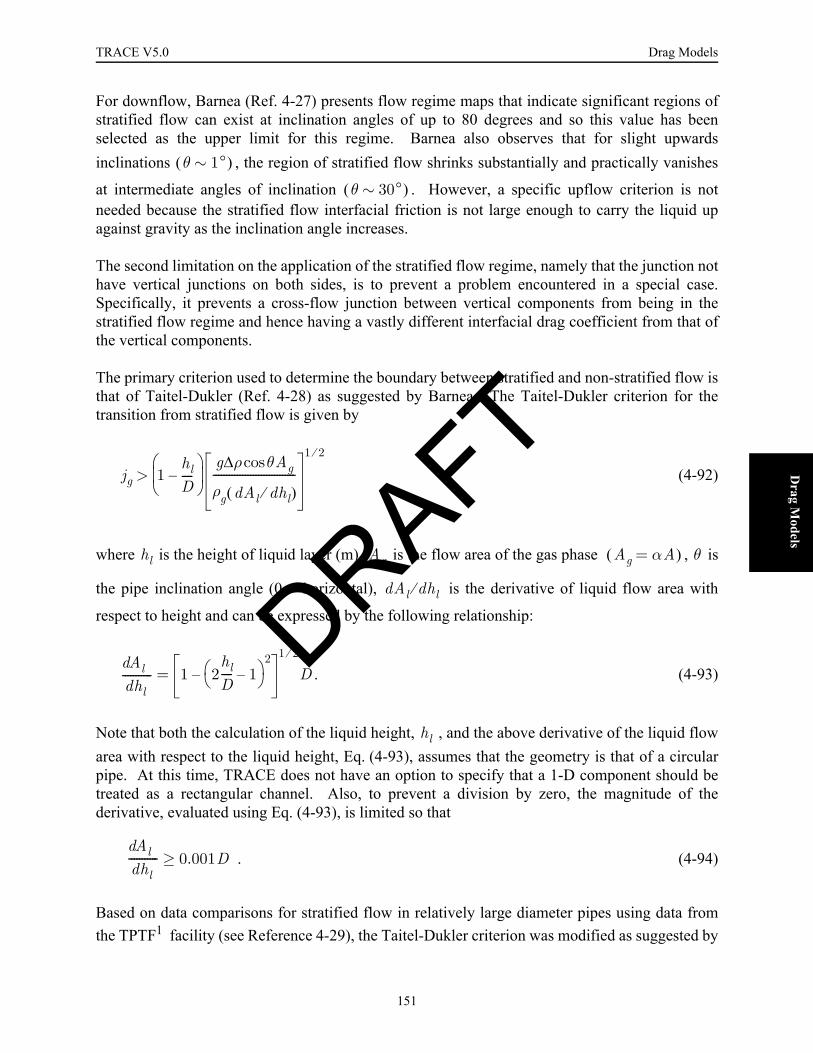
TRACE V5.0 Drag Models FOOBAR1234FOOBAR1234FOOBAR1234
Drag M
odels
For downflow, Barnea (Ref. 4-27) presents flow regime maps that indicate significant regions ofstratified flow can exist at inclination angles of up to 80 degrees and so this value has beenselected as the upper limit for this regime. Barnea also observes that for slight upwardsinclinations , the region of stratified flow shrinks substantially and practically vanishes
at intermediate angles of inclination . However, a specific upflow criterion is notneeded because the stratified flow interfacial friction is not large enough to carry the liquid upagainst gravity as the inclination angle increases.
The second limitation on the application of the stratified flow regime, namely that the junction nothave vertical junctions on both sides, is to prevent a problem encountered in a special case.Specifically, it prevents a cross-flow junction between vertical components from being in thestratified flow regime and hence having a vastly different interfacial drag coefficient from that ofthe vertical components.
The primary criterion used to determine the boundary between stratified and non-stratified flow isthat of Taitel-Dukler (Ref. 4-28) as suggested by Barnea. The Taitel-Dukler criterion for thetransition from stratified flow is given by
(4-92)
where is the height of liquid layer (m), is the flow area of the gas phase , is
the pipe inclination angle (0 = horizontal), is the derivative of liquid flow area with
respect to height and can be expressed by the following relationship:
. (4-93)
Note that both the calculation of the liquid height, , and the above derivative of the liquid flowarea with respect to the liquid height, Eq. (4-93), assumes that the geometry is that of a circularpipe. At this time, TRACE does not have an option to specify that a 1-D component should betreated as a rectangular channel. Also, to prevent a division by zero, the magnitude of thederivative, evaluated using Eq. (4-93), is limited so that
. (4-94)
Based on data comparisons for stratified flow in relatively large diameter pipes using data fromthe TPTF1 facility (see Reference 4-29), the Taitel-Dukler criterion was modified as suggested by
θ 1°∼( )
θ 30°∼( )
jg 1hlD----–
⎝ ⎠⎜ ⎟⎛ ⎞ g ρ θAgcos∆
ρg dAl dhl⁄( )-------------------------------
1 2⁄
>
hl Ag Ag αA=( ) θ
dAl dhl⁄
dAl dhl----------- 1 2
hlD---- 1–⎝ ⎠
⎛ ⎞2
–1 2⁄
D=
hl
dAl dhl----------- 0.001D≥
DRAFT
151
Drag Models TRACE V5.0
Anoda et. al. (Ref. 4-30). That is, the superficial gas velocity in Eq. (4-92) was replaced by therelative velocity, so that the criterion becomes
(4-95)
Using the value of the critical relative velocity from Eq. (4-95), a weighting factor for the Taitel-Dukler transition from stratified flow is defined
(4-96)
where a value of unity indicates that stratification is possible and zero that the flow isnon-stratified. The usage of the stratified flow weighting factor is explained in Transition toNon-Stratified Flow, and its effectiveness in predicting the void fraction for co-current horizontalflow is illustrated in Figure 4-10. This figure presents the results of a TRACE assessment caseagainst the TPTF horizontal flow tests (Ref. 4-29) for a pipe with a diameter of 0.18 m.
Two additional criteria are used to determine whether the flow can be stratified:
• the flow regime transition criterion for dispersed bubbly flow, and
• the counter-current flow limit (CCFL) for inclined pipes.
Each of these criteria and its TRACE implementation are described below.
For high liquid flow rates, liquid phase turbulence can break-up the gas phase into small dispersedbubbles. Choe et. al. (Ref. 4-31) gave the criterion for this transition to homogeneous dispersedbubbly flow as a simple mass flux limit. They concluded that homogeneous flow begins at
(4-97)
or
(4-98)
The implementation of this criterion is taken from the TRAC-PF1/Mod2 flow regime map (Ref.4-32) and the corresponding weighting factor is defined by
1. TPTF - the Two-Phase Test Facility operated in conjunction with the ROSA program by the Japan Atomic Energy Research Institute, located in Tokai, Japan.
Vr crit,
1hlD----–⎝ ⎠
⎛ ⎞ g ρ θAgcos∆
ρg dAl dhl⁄( )-------------------------------
1 2⁄
=
wfT D– Max 0 Min 1 2Vr
Vr crit,
-----------------–,⎝ ⎠⎜ ⎟⎜ ⎟⎛ ⎞
,=
G 2 6×10 (lbm/ft2 hr)=
G 2700 (kg/m2 s )≈
DRAFT
152

TRACE V5.0 Drag Models FOOBAR1234FOOBAR1234FOOBAR1234
Drag M
odels
(4-99)
In building a TRACE input model, the user has the responsibility of specifying geometrydependent CCFL model coefficients at all significant flow area restrictions where CCFL isexpected to occur. However, CCFL can also occur, and be important, for components such as thehot leg of a PWR that do not have any significant flow area restrictions. To handle suchgeometries, without placing a needless burden on the user, the Richter CCFL model (Ref. 4-33)for inclined pipes was built into the stratification criteria of TRACE. Basically, the idea is that ifthe flooding criteria are exceeded, then the flow cannot be stratified and the increased interfacialdrag of the non-stratified regime will be sufficient to prevent counter-current flow.
The Richter CCFL model (Ref. 4-33) for inclined pipes was selected for implementation inTRACE due to its good representation of the full-scale hot leg CCFL tests in the UPTF1 facility(see Reference 4-34). It is expressed by:
Figure. 4-10. Comparison of calculated and measured void fractions for the TPTF co-current horizontal flow tests (Ref. 4-29).
1. The Upper Plenum Test Facility, for investigating three-dimensional flow phenomena at full-scale, mod-eled the upper plenum, loops and downcomer of a PWR and was the German contribution to the 2D/3D project.
wfC W– Max 0 Min 1 2700 G –2700 2000–------------------------------,
⎝ ⎠⎜ ⎟⎛ ⎞
,=
DRAFT
153

Drag Models TRACE V5.0
(4-100)
where
, and (4-101)
(4-102)
To implement this model in TRACE, a stratified weighting factor is defined as
(4-103)
This weighting factor is used to turn stratification off gradually as the sum, ,
increases from 0.65 to 1.2 and was found to give a good representation of the flooding curve forthe UPTF hot leg tests as illustrated in Figure 4-11.
In Eq. (4-100) and Eq. (4-103), it is assumed that the flow is counter-current and so it is themagnitude of the liquid superficial velocity that is used in Eq. (4-102). For co-current flowsituations, for the evaluation of the CCFL weighting factor, the liquid superficial velocity is takento be zero, and so Eq. (4-100) effectively becomes
(4-104)
and is applied as an upper limit for the gas velocity in co-current stratified flow. This approachwas adopted to provide a continuous treatment at the flooding point.
In summary, three separate criteria are used to determine whether or not the flow can be stratified:
• it must first satisfy the modified form of the Taitel-Dukler criterion (Eq. (4-95)) that represents the transition from stratified to intermittent flow,
• the mass flux must be low enough, see Eq. (4-98), so that the flow is not in the dispersed bubble regime, and
jg*1 2⁄
jl*1 2⁄
+ 0.7=
jg* jgρg
g ρD∆--------------
⎝ ⎠⎜ ⎟⎛ ⎞
1 2⁄
=
jl* jlρl
g ρD∆--------------
⎝ ⎠⎜ ⎟⎛ ⎞
1 2⁄
=
wfCCFL Max 0 Min 11.2 jg*
1 2⁄jl*1 2⁄
+⎝ ⎠⎛ ⎞–
1.2 0.65–----------------------------------------------------,,
⎩ ⎭⎪ ⎪⎪ ⎪⎨ ⎬⎪ ⎪⎪ ⎪⎧ ⎫
=
jg*1 2⁄
jl*1 2⁄
+⎝ ⎠⎛ ⎞
jg*1 2⁄
0.7=
DRAFT
154
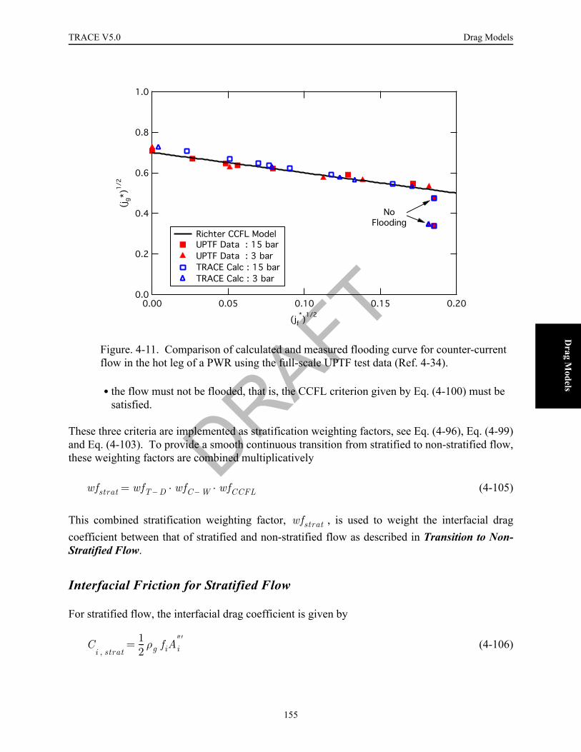
TRACE V5.0 Drag Models FOOBAR1234FOOBAR1234FOOBAR1234
Drag M
odels
• the flow must not be flooded, that is, the CCFL criterion given by Eq. (4-100) must be satisfied.
These three criteria are implemented as stratification weighting factors, see Eq. (4-96), Eq. (4-99)and Eq. (4-103). To provide a smooth continuous transition from stratified to non-stratified flow,these weighting factors are combined multiplicatively
(4-105)
This combined stratification weighting factor, , is used to weight the interfacial dragcoefficient between that of stratified and non-stratified flow as described in Transition to Non-Stratified Flow.
Interfacial Friction for Stratified Flow
For stratified flow, the interfacial drag coefficient is given by
(4-106)
Figure. 4-11. Comparison of calculated and measured flooding curve for counter-current flow in the hot leg of a PWR using the full-scale UPTF test data (Ref. 4-34).
!"
!"
#$
wfstrat wfT D– wfC W– w· fCCFL·=
wfstrat
Ci strat,
12--- ρg fiAi
″′=
DRAFT
155

Drag Models TRACE V5.0
where the interfacial area per unit volume is
(4-107)
and is the width of the stratified two-phase interface as depicted in Figure 4-12.
The only stratified flow regime that is explicitly modeled is the "stratified smooth" regime wherethe phases flow separately with a relatively smooth interface. To specify the interfacial frictionfactor for this regime, the correlation of Ohnuki et. al. (Ref. 4-35) that was used in TRAC-PF1/Mod2 is retained. The interfacial friction factor is then given by
(4-108)
where is the single-phase wall drag friction factor for the gas phase. The wall-gas frictionfactor is evaluated as a function of the gas Reynolds no. using the formula of Churchill (Ref. 4-36). This is given in the section Single-Phase Friction Factor below. The gas phase Reynoldsno. is computed from
, (4-109)
Figure. 4-12. Schematic of stratified flow in a horizontal pipe.
Ai″′ Si
A----=
Si
fi 1.84 fwg·=
fwg
Regρg VgDgµg
-----------------------=
DRAFT
156

TRACE V5.0 Drag Models FOOBAR1234FOOBAR1234FOOBAR1234
Drag M
odels
where is a special hydraulic diameter for the gas-phase computed for stratified flow assuggested by Agrawal et. al. (Ref. 4-37):
(4-110)
where is the perimeter of the pipe in the gas region (see Figure 4-12).
Transition to Non-Stratified Flow
The stratified flow weighting factor, , introduced in Eq. (4-105), is used to weight thecontributions to the interfacial drag from the stratified and non-stratified flow regimes. Becausethe respective interfacial drag coefficients for these disparate regimes can vary by several ordersof magnitude, an exponential weighting scheme is used. Thus, when the stratified flow weightingfactor is greater than zero, the interfacial drag coefficient is given by
(4-111)
where the exponent, , is set equal to .
Post-CHF Interfacial Drag Models
When the temperature of a surface is above the Leidenfrost1 point, the liquid phase cannot contactthe hot surface. This gives rise to a family of "inverted" flow regimes with the gas phase incontact with the wall as depicted schematically in Figure 4-13. The determination between thenormal pre-CHF flow regimes and the inverted post-CHF flow regimes is made using the axiallocations of the bottom and top quench fronts. For momentum cells that are completelyquenched, the normal pre-CHF regimes are used. Whereas, for momentum cells whose heattransfer surface is in film boiling, (i.e., they are located entirely between the top and bottomquench fronts), the inverted post-CHF flow regimes are used. Finally, for cells that are partiallyquenched, an interpolation between the interfacial drag coefficients for the pre- and post-CHFvalues is performed as explained in Transition to Pre-CHF Regimes.
Three principal inverted flow regimes are modeled in TRACE for post-CHF conditions: invertedannular, inverted slug, and dispersed flow. The region over which each of these post-CHF flowregimes is applied is shown in Figure 4-14. This post-CHF flow regime map is primarily afunction of the void fraction with the gas superficial velocity governing the entrainment fraction
1. This temperature is also commonly known as , which is short for the "minimum stable film boiling
temperature".
Dg
Dg4Ag
Sg Si+( )------------------------=
Sg
wfstrat
Ci C ni strat, C 1 n–( )
i ns,·=
n wfstrat
Tmin
DRAFT
157

Drag Models TRACE V5.0
and hence the transition to dispersed flow. The models used for the evaluation of the interfacialdrag coefficient for each of these flow regimes, as well as the flow regime transition criteria aredescribed in the following sections.
Inverted Annular
The inverted annular flow regime typically occurs when subcooled liquid flows past the quenchfront. Just downstream of the quench front, a thin vapor film separates the liquid core from thehot wall. Initially, the vapor velocity is low so that the flow is laminar and the gas-liquid interfaceis smooth. Further downstream of the quench front, as the subcooling of the liquid core is
Figure. 4-13. Schematic of the inverted flow regimes that occur for post-CHF conditions.
DRAFT
158

TRACE V5.0 Drag Models FOOBAR1234FOOBAR1234FOOBAR1234
Drag M
odels
reduced, the vapor flow increases causing the interface to first become wavy and then oscillateviolently until breakup occurs at about the point where the liquid becomes saturated.Experimental data indicate that the inverted annular regime persists up to void fractions of 60-70% and that a smooth transition, in so far as the wall heat transfer is concerned, is made to thedispersed flow regime. In TRACE, the inverted annular regime is assumed to exist for voidfractions up to 60%.
For the inverted annular regime, the interfacial drag coefficient is given by
(4-112)
where the interfacial area per unit volume is computed from the void fraction assuming that theliquid core is circular, that is
(4-113)
When the gas film flow is laminar, the interfacial friction factor is assumed equal to that for flowbetween parallel plates, namely
(4-114)
Figure. 4-14. Post-CHF flow regime map.
Ci IA,
12---ρgfiAi
″′=
Ai″′ 4 1 α–( )
Dh---------------------=
fi 24Reg---------=
DRAFT
159

Drag Models TRACE V5.0
where the gas phase Reynolds no. is defined by
(4-115)
Cachard (Ref. 4-38) introduced a non-dimensional gas film thickness for the analysis of invertedannular film boiling, given by
(4-116)
and used it as the correlating parameter for the interfacial friction factor. For laminar flow with asmooth interface, Eq. (4-114) can then be recast as
(4-117)
and it is this formulation that is used in TRACE.
As the gas flow increases, the flow becomes turbulent and the interface becomes wavy orirregular causing the friction factor to increase. To complete the specification for the interfacialfriction factor for the inverted annular regime, it remains to define the friction factor for this wavyregime.
Although void fraction measurements exist for inverted annular flow, because the flow quality isnegative, the actual phasic velocities are unknown and it is impossible to directly determine theinterfacial friction from this data. Consequently, a simple model has been developed thatdescribes the correct qualitative behavior. This model is an inverted analog to that for annularflow. Specifically, the interfacial friction factor is taken to be a function of the interfaceroughness and this roughness is assumed to be proportional to the thickness of the gas film.
From observations on ducts with grooved or wavy walls, the friction factor follows that of smoothparallel plates up to a Reynolds no. of about 200-400. With further increases in the Reynolds no.,significant flow separation is observed and the friction factor versus Reynolds no. curve takes onthe appearance of that for fully rough turbulent flow. That is, it is nearly a constant value with themagnitude of that value dependent upon the amplitude/wavelength ratio. From this observation,and that of Andritsos and Hanratty (Ref. 4-39) that the interfacial friction factor for horizontalstratified flow is dependent on the wave amplitude and consequently is linearly proportional tothe vapor Reynolds no., the following model was developed:
. (4-118)
Regαρg VgDhµg
---------------------------=
δ* δρgg ρ∆
µg2
---------------1 3⁄
=
fi smooth,
144
δ*( )3
------------=
fi wavy,
0.35 δLa-------
⎝ ⎠⎜ ⎟⎛ ⎞
0.72
=
DRAFT
160

TRACE V5.0 Drag Models FOOBAR1234FOOBAR1234FOOBAR1234
Drag M
odels
The exponent in the above formula was selected so that the interfacial friction factor, when wavesgovern its value, is linearly proportional to the vapor Reynolds no. The Laplace no., given by
(4-119)
was used to non-dimensionalize the gas film thickness in order to provide a continuous treatmentwith that for the inverted slug regime. Finally, the approximate value of the coefficient inEq. (4-118) was determined from data comparisons with FLECHT-SEASET high flooding ratereflood data.
Rather than try to specify a criterion for the transition from smooth to wavy inverted annular flow,a power law weighting was used. Specifically,
(4-120)
The resulting model for the interfacial friction factor in the inverted annular flow regime isdepicted in Figure 4-15. The minimum value of the friction factor occurs at a gas Reynolds no. ofabout 350 followed by an increase that is linearly proportional to the Reynolds no.
Figure. 4-15. Interfacial friction factor for the inverted annular flow regime as a function of the gas Reynolds no.
La σg ρ∆---------=
fi IA,
f 2i smooth, f 2
i wavy,+1 2⁄
=
DRAFT
161
Drag Models TRACE V5.0
Inverted Slug Regime
Further downstream of the quench front, as the subcooling of the liquid core is reduced, the vaporflow increases causing the interface to first become wavy and then oscillate violently untilbreakup occurs at about the point where the liquid becomes saturated. Kawaji and Banerjee (seeReference 4-40) observed that the wavelength of maximum growth rate was about 4.5 times thediameter of the liquid column. Therefore, they proposed that the ligaments formed by thedisintegration of the inverted annular core could be modeled as prolate ellipsoids with the lengthof the semi-major axis larger than that of the semi-minor axis by a factor of 4.5. This proposal,coupled with the fluidized bed concept, form the basis for the inverted slug flow regime model inTRACE.
For the inverted slug regime, the interfacial drag coefficient is given by
(4-121)
where is the drag coefficient corrected for multi-particle effects and is the projected
area per unit volume. Based on the assumption that the ligaments can be represented as prolateellipsoids, the projected area of a ligament would be
(4-122)
and its volume would be
(4-123)
where and are the minor and major radii of the ellipsoid respectively. With an aspect ratio of4.5, the projected area per unit volume becomes
(4-124)
where is the diameter of the ligament, that is twice the minor radius.
To estimate the drag coefficient for a ligament, the formula for a distorted droplet given by Clift,Grace and Weber (Ref. 4-41) is used. The single particle drag coefficient is then
(4-125)
Ci IS,
12---ρgCD MP,
Ap″′=
CD MP,
Ap″′
Ap πa2=
V 43---πa2b=
a b
Ap″′ 1 α–( )
3dIS-----------------=
dIS
CD SP,
13---
dISLa-------
⎝ ⎠⎜ ⎟⎛ ⎞
=
DRAFT
162
TRACE V5.0 Drag Models FOOBAR1234FOOBAR1234FOOBAR1234
Drag M
odels
The multi-particle effect is taken to be that of the inertial regime from Richardson and Zaki (Ref.4-42), that is
(4-126)
Combining Eq. (4-124) through Eq. (4-126), we have
(4-127)
In TRACE, the above interfacial drag coefficient has been reduced by a factor of ¾ to bettermatch FLECHT-SEASET high flooding rate reflood data, so that
(4-128)
As indicated in Figure 4-14, an interpolation region is applied between the inverted annular andinverted slug flow regimes. The rationale for this interpolation region is that film boiling heattransfer data indicates a smooth transition between these two regimes. Consequently, aninterpolation region was used for the wall heat transfer coefficient and the same interpolationscheme is used here for consistency.
For void fractions less than 60%, the flow regime is inverted annular, whereas for void fractionsabove 90%, the flow regime is inverted slug. At void fractions between these limits, theinterfacial drag coefficient is computed from
(4-129)
where is a spline weighting factor for inverted annular flow. This weighting factor is givenby
(4-130)
where
(4-131)
This completes the description of the models used for the inverted slug flow regime. As the gasvelocity increases, entrainment becomes important and a transition to the dispersed flow regimeoccurs as described in the following section.
CD MP,
CD SP ,
α1.8--------------------=
Ci IS,
118------
ρgLa------- 1 α–( )
α1.8-----------------=
Ci IS,
124------
ρgLa------- 1 α–( )
α1.8-----------------=
Ci wfIA Ci IA,
+ (1 wfIA ) Ci IS,
·–·=
wfIA
wfIA x (2 x )–=
x (0.9 α )– (0.9 0.6 )–------------------------------=
DRAFT
163

Drag Models TRACE V5.0
Dispersed Flow
After the breakup of the inverted annular core, the liquid phase is assumed to consist of ligamentsand droplets. The ligaments are treated as prolate ellipsoids as described in Inverted SlugRegime. The droplets are relatively small and nearly spherical, so they are treated using modelsappropriate for spheres.
The interfacial drag coefficient for the dispersed flow regime is
(4-132)
where the projected area per unit volume is calculated from the droplet Sauter mean diameter by
(4-133)
Four specific constitutive models are needed to evaluate of the dispersed flow regime:
•Droplet diameter,
•Droplet drag coefficient,
•Multiple particle effect, and
•Entrained fraction.
Each of these four models is detailed below, along with the interpolation scheme used for thetransition from inverted slug to dispersed flow.
As the gas velocity increases and ligaments shatter, both large liquid fragments and small dropletsare formed. It is assumed that the creation of these small droplets is due to the Kelvin-Helmholtzinstability, and hence a Weber no. criterion is used to estimate their initial diameter. Themaximum droplet diameter is then
(4-134)
where a critical value of 12 was chosen for the Weber no. The relative velocity in the denominatorof Eq. (4-134) is evaluated using the droplet terminal velocity. Wallis (Ref. 4-43) gives theterminal velocity for large spherical drops (Region 2B in (Ref. 4-43)) as
(4-135)
where the non-dimensional values of the velocity and droplet radius are defined as
Ci DF,
12--- ρgCD MP,
Ap″′=
Ap″′ 6(1 α )–
4dSM-------------------------=
Ci DF,
d max12σ
ρg V r2
------------------=
V *∞ 0.693 r*( )
0.858=
DRAFT
164
TRACE V5.0 Drag Models FOOBAR1234FOOBAR1234FOOBAR1234
Drag M
odels
, and (4-136)
(4-137)
Eq. (4-135) is valid for the range, , which covers the expected size range for dropdiameters during reflood. Combining Eq. (4-134) and Eq. (4-135) yields
(4-138)
for the initial maximum droplet diameter as a function of the Laplace and Viscosity nos.
Further downstream, as the gas velocity increases, additional droplet breakup due to the Kelvin-Helmholtz instability may occur. Here, it is assumed that the largest drops are only just levitatedby the gas stream and that for the dispersed flow region the void fraction is near unity, so therelative velocity is approximated by the gas superficial velocity,
(4-139)
The critical Weber no. criterion then becomes
(4-140)
In TRACE, for the subsequent breakup of drops in the dispersed flow regime, the value of thecritical Weber no., , was set to 18 to better match dispersed flow film boiling heat transferdata in the THTF upflow film boiling tests. Thus,
(4-141)
The local value for the maximum drop diameter is then taken as the minimum of the two valuesgiven by Eq. (4-138) and Eq. (4-141), that is
(4-142)
V *∞ V∞
ρg2
µgg ρ∆----------------
1 3⁄
=
r* rρgg ρ∆
µg2---------------
1 3⁄
=
10 r* 36< <
d max 5.07 La N 0.176µg··=
Vr jg≈
dWeWecrit σ
ρg jg2
-----------------------=
Wecrit
dWe18σρg jg
2--------------=
d max Min 5.07 La N0.176µg
18σρg jg
2--------------
⎝ ⎠⎜ ⎟⎛ ⎞,··=
DRAFT
165

Drag Models TRACE V5.0
Eq. (4-142) is used for the maximum drop diameter for upflow cases, .
For downflow, , the assumptions used to estimate the drop relative velocity in Eq. (4-138)and Eq. (4-141) do not apply, as the drops can fall freely with the gas stream. Consequently, adifferent criterion is used for the maximum droplet diameter, that is, the drop size is assumed tobe governed by the Rayleigh-Taylor instability and the physical dimensions of the flow channel.Kitscha and Kocamustafaogullari (Ref. 4-44) give the Rayleigh-Taylor limit, for freely fallingdrops in a gaseous media, as
(4-143)
and, since the largest drop cannot be larger than the flow channel,
(4-144)
For upflow conditions, the maximum diameter given by Eq. (4-142) should always besignificantly smaller than that given by Eq. (4-144). However, for consistency, the value fromEq. (4-144) is also applied as an upper limit on the drop size.
Finally, for the estimation of the projected area per unit volume, the relationship between themaximum diameter and the Sauter mean diameter is needed. Ardron and Hall (Ref. 4-45)observed that for their experimental droplet size distributions, the Sauter mean diameter wastypically about one-third of the maximum diameter and this ratio is used in TRACE. Thus,
(4-145)
The second step is to evaluate the droplet drag coefficient. As stated above, the dispersed dropletsare relatively small and nearly spherical, so the standard drag curve for spheres can be used. Clift,Grace and Weber (Ref. 4-46), provide a table of formulas that approximate the rigid sphere dragcurve. From this table, the formula of Schiller and Nauman was selected due to its high accuracyfor drop Reynolds nos. less than 800. The single-particle drag coefficient is then
(4-146)
where the drop Reynolds no. is defined by
(4-147)
jg 0>
jg 0<
dR T– 3.52La=
d max Min 3.52La Dh, =
dSM13--- d max=
CD SP,
24Red -------------- 1 + 0.15Re0.687
d⎝ ⎠⎛ ⎞=
RedρgVrdSMµ
g film,
----------------------=
DRAFT
166

TRACE V5.0 Drag Models FOOBAR1234FOOBAR1234FOOBAR1234
Drag M
odels
The relative velocity used in Eq. (4-147) is simply the magnitude of the difference between thephasic velocities, , but with the two modifications described below.
First, the phasic relative velocity results from the solution of the velocity equations using themulti-particle drag coefficient. To make it consistent with the Richardson and Zaki (Ref. 4-42)formulation, this relative velocity must be translated to that which would occur for a singleparticle in an infinite medium. Thus,
(4-148)
Then, to prevent unrealistically high values of the drag coefficient, this relative velocity is limitedto be larger than that given by Eq. (4-135) for the single-particle terminal velocity.
Note also that the gas viscosity in Eq. (4-147) is evaluated at a "film" temperature. This is toaccount for the mass transfer effect upon the drag coefficient as suggested by Renksizbulut andYuen (Ref. 4-47). The film temperature is defined by
(4-149)
to account for the surface of the droplet being at the saturation temperature and the variation ofproperties from the free stream value.
Finally, for drop Reynolds nos. greater than about 1000, the drag coefficient approaches aconstant value and may be approximated by
(4-150)
To provide a continuous treatment, the maximum of Eq. (4-146) and Eq. (4-150) is taken.
For the multi-particle effect, the inertial regime from Richardson and Zaki (Ref. 4-42) is used. Toimplement this model requires two modifications. The first was described above and modifies thedrop Reynolds no. used in the computation of the single-particle drag coefficient. The seconddirectly modifies the drag coefficient in the same manner as was done for the inverted slugregime, that is
(4-151)
The transition from the inverted slug to the dispersed flow regime is governed by the entrainmentfraction, that is, the fraction of the liquid determined to be entrained is treated as droplets while
Vg Vl–
VrVg Vl–
α1.4---------------------------=
Tfilm12--- Tg Tsat+( )=
CD SP,
0.44≈
CD MP,
CD SP ,
α1.8--------------------=
DRAFT
167

Drag Models TRACE V5.0
the remainder of the liquid is considered to be inverted slugs. To effect this transition, a simplelinear weighting scheme is employed,
(4-152)
where is the entrainment fraction.
The first step in determining the entrainment fraction is to specify a critical gas velocity for theonset of entrainment. This critical gas velocity is computed from Eq. (4-135) to be consistentwith the formula for the drop diameter. The critical gas superficial velocity is then that which isjust sufficient to levitate a drop with the Sauter mean diameter given by Eq. (4-138) andEq. (4-145). Thus,
(4-153)
For superficial gas velocities less than this value, the entrainment fraction will be zero and theflow regime will be inverted slug.
For higher gas velocities, the entrainment fraction is estimated using a modified form of the poolentrainment correlation of Kataoka and Ishii (Ref. 4-48). They express the entrained liquid massflux as a function of a critical non-dimensional gas velocity and the gas mass flux by
(4-154)
where the non-dimensional gas superficial velocity is defined
(4-155)
To make Eq. (4-154) consistent with the criterion for the onset of entrainment, two modificationsare made. First, it is recast in terms of the critical gas velocity as
(4-156)
which does not affect the magnitude of the entrained liquid mass flux. Then, to force theentrained fraction to zero at the critical value for the onset of entrainment, Eq. (4-156) is modifiedto
Ci E C·i DF,
1 E–( ) Ci IS,
·+=
E
jg crit,
0.6 σ0.316 g ρ∆( )0.228
ρg0.456 µg
0.0879---------------------------------------=
Gd 0.002 jg*3Nµg
1 2⁄ ρ∆ρg------
⎝ ⎠⎜ ⎟⎛ ⎞
Gg=
jg* jg
ρgσg ρ∆-------------
2
⎝ ⎠⎜ ⎟⎛ ⎞ 1 4⁄
=
Gd 4.32 4–×10 jg
jg crit,
---------------⎝ ⎠⎜ ⎟⎛ ⎞ 3
Nµg0.236 ρ∆
ρg------
⎝ ⎠⎜ ⎟⎛ ⎞
Gg=
DRAFT
168
TRACE V5.0 Drag Models FOOBAR1234FOOBAR1234FOOBAR1234
Drag M
odels
(4-157)
or more simply to
(4-158)
Based on reflood data comparisons with TRACE, the value for the entrained mass flux given byEq. (4-158) above is reduced by a factor of two. So,
(4-159)
The last step is to convert the entrained mass flux into the entrainment fraction and by definition
(4-160)
which is expressed in TRACE as
(4-161)
where the droplet volume fraction is estimated from
(4-162)
This completes the description of the models necessary to determine the interfacial dragcoefficient for the dispersed flow regime and for the transition regime between dispersed flow andinverted slug flow. The following section describes the transition from the post-CHF regimes tothe normal pre-CHF flow regimes.
Transition to Pre-CHF Regimes
The determination between the normal pre-CHF flow regimes and the inverted post-CHF flowregimes is made using the axial locations of the bottom and top quench fronts. For momentum
Gd 4.32 4–×10 jg
jg crit,
---------------⎝ ⎠⎜ ⎟⎛ ⎞ 3
1– Nµg0.236 ρ∆
ρg------
⎝ ⎠⎜ ⎟⎛ ⎞
Gg=
Gd 4.32 4–×10 jg
jg crit,
---------------⎝ ⎠⎜ ⎟⎛ ⎞ 3
1– Nµg0.236 ρ∆ jg=
Gd 2.16 4–×10 jg
jg crit,
---------------⎝ ⎠⎜ ⎟⎛ ⎞ 3
1– Nµg0.236 ρ∆ jg=
EGdGl-------=
Eαd
1 α–( )-----------------=
αdGd
ρl Max 0.01 Vl,( )·------------------------------------------------≈
DRAFT
169

Drag Models TRACE V5.0
cells that are completely quenched, the normal pre-CHF regimes are used. Whereas, formomentum cells whose heat transfer surface is in film boiling, (i.e., they are located entirelybetween the top and bottom quench fronts), the inverted post-CHF flow regimes are used.Finally, for cells that are partially quenched, an exponential interpolation between the interfacialdrag coefficients for the pre- and post-CHF values is performed.
Let represent the fraction of the momentum cell that is quenched. Then,
(4-163)
where the exponential interpolation is used because of the large difference in the magnitude of thepre- and post-CHF interfacial drag coefficients. This helps to reduce the perturbation that occursas the quench front crosses a cell boundary.
The description of the interfacial drag models is complete, the single-phase and two-phase walldrag models are described next.
Wall DragTwo types of frictional pressure losses are modeled in TRACE:
•Wall Drag: models the fluid-wall shear using a friction factor approach, and
•Form Drag: models geometry specific pressure losses through user specification of additive loss coefficients" for irreversible form losses due to abrupt or semi-abrupt flow-area expansions and contractions, thin-plate-orifice-type flow restrictions, and flow redirection (turning) at an elbow or tee.
The models for both single- and two-phase wall drag are described in the following sections. TheTRACE model for additive loss coefficients is described in Chapter 7.
In the TRACE formulation, the frictional pressure gradient due to wall drag is given by:
(4-164)
where and are the wall drag coefficients for wall-liquid and wall-gas shear respectively.Typically, only one of these coefficients has a non-zero value. For example, in either bubbly/slugor annular/mist flow, all of the wall drag is applied to the liquid phase and is set to zero.
For TRACE, the wall drag model from TRAC-PF1/MOD2 was substantially modified to:
• Improve accuracy in the annular flow regime so that film thickness can be calculated accurately, especially for applications in downflow condensers, and
fQ
Ci Ci( )pre CHF–fQ Ci( )post CHF–
1 fQ–( )·=
dPdz-------
f C– wl Vl Vl Cwg Vg Vg · ·–··=
Cwl Cwg
Cwg
DRAFT
170
TRACE V5.0 Drag Models FOOBAR1234FOOBAR1234FOOBAR1234
Drag M
odels
•Explicitly account for the post-CHF "inverted" flow regimes where the only wall-fluid contact is to the gas phase.
Four specific areas of application for the wall drag model are discussed below: single-phasefraction factor, pre-CHF regimes, horizontal stratified flow, and post-CHF regimes.
Single-Phase Friction Factor
For single-phase flow, the wall drag coefficient is defined by
(4-165)
where the subscript indicates the fluid phase ( l or g ) and is the Fanning friction factor1 .The Churchill formula (see Reference 4-36) for the friction factor is used in TRACE because itapplies to all three flow regimes - laminar, transition, and turbulent.
The Churchill friction factor formula is given by
(4-166)
where
(4-167)
and
(4-168)
1. The Darcy friction factor is four times larger than the Fanning friction factor.
Cwk fwk4
Dh------- 1
2---ρk· · fwk
2ρkDh--------·= =
k fw
fw 2 8Re-------
⎝ ⎠⎜ ⎟⎛ ⎞12 1
a b+( )3 2⁄
------------------------+1 12⁄
=
a 2.475
1
7Re-------
⎝ ⎠⎜ ⎟⎛ ⎞
0.9
0.27 εDh-------
⎝ ⎠⎜ ⎟⎛ ⎞
+
--------------------------------------------------ln·
⎩ ⎭⎪ ⎪⎪ ⎪⎪ ⎪⎨ ⎬⎪ ⎪⎪ ⎪⎪ ⎪⎧ ⎫16
=
b 3.753 4×10 Re
-------------------------⎝ ⎠⎜ ⎟⎛ ⎞
16
=
DRAFT
171

Drag Models TRACE V5.0
Its predictions for the laminar regime are in agreement with , as expected. Thepredictions for transition flow are subject to some uncertainty (as indeed is the experimental datafor this regime). However, according to Reference 4-49, its accuracy for turbulent flow shows amaximum deviation from the Colebrook-White equation of about 3.2% for 4000 < Re < 108 and
10-8 < < 0.05. A simplified Moody diagram created using the Churchill equation ispresented in Figure 4-16.
In Eq. (4-166), the Reynolds no. is computed for the phase of interest by
(4-169)
and, to eliminate very large values for nearly stagnant conditions, is limited to be greater than 10.
In TRACE, there is no specific test for single-phase liquid wall drag. Instead, the two-phasemodel for the bubbly/slug regime devolves into the single-phase value as the limit of zero voidfraction is approached. In contrast, as the void fraction approaches unity, an explicit ramp is
Figure. 4-16. Representation of the Moody diagram using the Churchill friction factor formula Eq. (4-166).
fw 16 Re⁄=
ε D⁄
Rek
ρk Vk Dh
µk------------------------=
DRAFT
172

TRACE V5.0 Drag Models FOOBAR1234FOOBAR1234FOOBAR1234
Drag M
odels
applied to switch the wall drag from the liquid to the gas phase. This ramp is explained inAnnular Flow Regime.
Pre-CHF Regimes: Two-Phase Multiplier
For the normal pre-CHF flow regimes, bubbly/slug and annular/mist, all of the wall drag isapplied to the liquid phase alone. Thus,
(4-170)
or, in terms of the two-phase multiplier for the liquid phase considered to flow alone in thechannel,
(4-171)
where the friction factor, , is the Fanning friction factor1 calculated with
(4-172)
The wall drag coefficient is then
(4-173)
To complete the specification of the wall drag for the pre-CHF regimes, it remains to specify the
two-phase multiplier, , and the friction factor, . The annular flow regime is treated first
because:
1. Note, the double subscript, " ", is used to differentiate the liquid friction factor for two-phase condi-tions for the liquid phase considered to flow alone in the channel, , from the single-phase liquid
friction factor, . The primary difference between these two is the definition of the liquid Reynolds
no. (see Eq. (4-169) and Eq. (4-172)) used to evaluate them.
dPdz-------
f C– wl Vl Vl ·=
dPdz-------
fΦl
22f
2Φ l,Gl Gl
Dh ρl--------------------------------–=
f2Φ l,
2Φ l,f2Φ l,
fwl
Re2Φ l,
Gl Dhµl
----------------1 α–( )ρl Vl Dh
µl---------------------------------------= =
Cwl Φl2
2f2Φ l,
1 α–( )2ρl
Dh-----------------------------------------=
Φl2 f
2Φ l,
DRAFT
173

Drag Models TRACE V5.0
• improving accuracy for this regime was the reason for the modification to the wall drag model of TRACE, and
• its derivation is more straightforward than that for the bubbly/slug regime.
Following the description of the annular flow regime, the model for the bubbly/slug regime andthe transition between these two regimes are described.
Annular Flow Regime
The two-phase multiplier for the annular flow regime will be described first, followed by thedetermination of the friction factor for both the laminar and turbulent regimes. Finally, themodifications to account for the transition to single-phase gas flow as the void fractionapproaches unity are described.
Annular flow theory (see References 4-50 and 4-51) gives the two-phase multiplier as
(4-174)
Eq. (4-174) has been shown to give excellent predictions of the frictional pressure gradient whenthe friction coefficient is adjusted in the transition regime, as depicted in Figure 4-18. Forexample, see Figure 4-17 for a comparison of the annular flow two-phase multiplier, , used byTRACE with data both for co-current upflow and downflow.
Substituting Eq. (4-174) into Eq. (4-173) simplifies the wall drag coefficient to:
(4-175)
The only difference between Eq. (4-165) for single-phase liquid flow and Eq. (4-175) for annularflow is the evaluation of the friction factor.
In Figure 4-18, the friction factor for the annular flow regime is given by a power lawcombination of the laminar and turbulent values:
(4-176)
where the laminar value is that for pipe flow
(4-177)
Φl2 1
1 α–( )2--------------------=
Φl
Cwl ffilm2ρlDh-------·=
ffilm f lam3 f turb
3+⎝ ⎠⎛ ⎞
1 3⁄=
f lam16
Re2Φ l,
------------------=
DRAFT
174

TRACE V5.0 Drag Models FOOBAR1234FOOBAR1234FOOBAR1234
Drag M
odels
and the turbulent value is given by Haaland's explicit approximation (Ref. 4-52) to the Colebrookequation
(4-178)
Note that the roughness effect has not been established conclusively for annular flow, it isincluded here to provide a continuous description with that for single-phase flow.
For laminar flow, Eq. (4-177) is appropriate for pipe flow. However, as the film thins, the frictionfactor is better approximated by that for a parallel plate, namely
(4-179)
Therefore, in TRACE, a simple void fraction ramp1 is used between the formulas given byEq. (4-177) and Eq. (4-179). Specifically, for void fractions greater than 99%, the parallel plateformula is used and for void fractions less than 95%, the pipe formula is used. In between thesevalues, the laminar friction factor is computed from
Figure. 4-17. Comparison of the TRACE annular flow model versus data.
!" #$% & ' ( )') *+,
- ( $ *+,
-% $ ( ./ *++,
01% $ ( $ *+,
# " #2 ( 3 *+,
.245 6 7 *,
f turb1
3.6 log106.9
Re2Φ l,
------------------ε D⁄3.7
----------⎝ ⎠⎜ ⎟⎛ ⎞
1.11
+·
⎩ ⎭⎪ ⎪⎨ ⎬⎪ ⎪⎧ ⎫--------------------------------------------------------------------------------------
2=
f lam24
Re2Φ l,
------------------=
DRAFT
175

Drag Models TRACE V5.0
(4-180)
The accuracy of the TRACE model to calculate liquid film thickness is demonstrated in Figure4-19 for falling liquid films.
The transition to single-phase gas flow is handled by considering the breakdown of the film intorivulets. Film breakdown is assumed to occur when the film thickness becomes less than a criticalvalue. Many different models of varying complexity are available to predict this minimum filmthickness depending upon flow orientation, and whether evaporation or condensation isoccurring. In TRACE, a simple constant value of 25 microns is used. The resulting rivulets arefurther assumed to have a thickness equal to this critical value, so that the fraction of the surfacein contact with the liquid phase is estimated by
1. Note, there is no theoretical basis for Eq. (4-180), the actual laminar friction factor depends on the veloc-ity profile within the liquid film and is a function of the gravitational and interfacial shear forces. This ramp merely forces it to the correct limiting values.
Figure. 4-18. Comparison of friction factor for a film with that for a smooth pipe.
f lam
16 8 α 0.95–0.99 0.95–---------------------------
⎝ ⎠⎜ ⎟⎛ ⎞
+
Re2Φ l,
----------------------------------------------------------= DRAFT
176
TRACE V5.0 Drag Models FOOBAR1234FOOBAR1234FOOBAR1234
Drag M
odels
(4-181)where the thin film approximation has been used. The wall-liquid drag coefficient then becomes
(4-182)
For the fraction of the surface not covered by rivulets, wall drag is applied to the gas phase usingthe friction factor from Eq. (4-166) and
(4-183)
This completes the description for the annular flow regime, a similar "void fraction based" two-phase multiplier is used for the bubbly/slug flow regime as detailed below.
Figure. 4-19. Comparison of TRACE calculated values for film thickness with falling film data.
fwet1 α–( )Dh
4 25 6–×10( )----------------------------≈
Cwl fwet ffilm2ρlDh-------· ·=
Cwl 1 fwet–( ) f2Φ g,
2ρgDh--------· ·=
DRAFT
177

Drag Models TRACE V5.0
Bubbly/Slug Flow Regime
To also improve the accuracy of TRACE's wall drag model for the bubbly/slug regime, a two-phase multiplier was implemented as described below. Most correlations from the literature usethe flow quality as the primary correlating variable. However, as flow quality is undefined ormeaningless for a number of situations encountered in transient reactor analysis, such as counter-current flow and pool boiling, it is not an ideal correlating variable for a model in TRACE.Consequently, a "void fraction based" two-phase multiplier model was developed.
First, it was observed that the original Lockhart and Martinelli model (Ref. 4-53) tabulated values
for , almost exactly reproduce Eq. (4-174). However, in comparisons with two-phasepressure drop data, it was found that this expression over-estimated the two-phase multiplier.Indeed, using the adiabatic steam-water data of Ferrell & McGee (Ref. 4-54), one obtains
(4-184)
as shown in Figure 4-20.
This behavior of the two-phase multiplier with respect to the liquid fraction given by Eq. (4-184)is very similar to values reported by Yamazaki & Shiba (Ref. 4-55) and Yamazaki & Yamaguchi
Figure. 4-20. Liquid-only two-phase multipliers inferred from the adiabatic steam-water data of Ferrel-McGee (Ref. 4-54)
Φl2
Φl2 1
1 α–( )1.72--------------------------≈
DRAFT
178
TRACE V5.0 Drag Models FOOBAR1234FOOBAR1234FOOBAR1234
Drag M
odels
(Ref. 4-56) who suggested exponents of -1.75 for upflow and -1.8 for downflow. Especiallynotable is that when the data are represented this way there is no noticeable effect of mass flux,pressure or tube diameter.
Recall that for turbulent pipe flow, the friction factor varies roughly as to . Then,using the model for single-phase liquid flow Eq. (4-165) and Eq. (4-166) and a Reynolds no.defined by Eq. (4-169), gives an effective two-phase multiplier of
(4-185)
in line with experimental observations for adiabatic two-phase flow. This simple model for thetwo-phase multiplier was adopted for use in TRACE for the bubbly-slug flow regime.
For two-phase flows with nucleate boiling, the situation is more complicated than that discernedabove for adiabatic flows. The pressure drop data of Ferrell & Bylund (Ref. 4-57) show that thetwo-phase multiplier when boiling is present is both significantly higher and contains apronounced mass flux effect, as shown in Figure 4-21. No available model for the two-phasemultiplier specifically addresses the enhancement due to wall nucleation evident in this data.Collier (Ref. 4-58) does discuss a surface roughness effect for subcooled boiling and suggests thatit might be correlated in terms of the bubble departure diameter but does not extend this conceptinto the saturated boiling regime. Ferrell & Bylund's data covers both subcooled and saturatedboiling, yet there is no evident discontinuity in the behavior of the two-phase multiplier versusliquid fraction as the saturation line is crossed.
Consequently, a simple correction factor to the two-phase multiplier for adiabatic two-phase flowhas been developed using the data of Ferrell & Bylund in the form:
(4-186)
As suggested by Collier, it was postulated that this correction factor would be a function of thebubble departure diameter. Collier also suggests using the model developed by Levy (Ref. 4-59)that balances surface tension and drag forces to give
(4-187)
where the wall shear stress is computed without the enhancement due to wall nucleation. Thus,
(4-188)
Re 0.25– Re 0.2–
Φl2 1
1 α–( )1.75-------------------------- to 1
1 α–( )1.8-----------------------∼
Φl′ Φl 1 CNB+⎝ ⎠
⎛ ⎞·=
dgD-----
h0.015
στw Dh·-----------------
12---
·=
τw
f2Φ l,
2-------------- ρl Vl
2· ·=
DRAFT
179
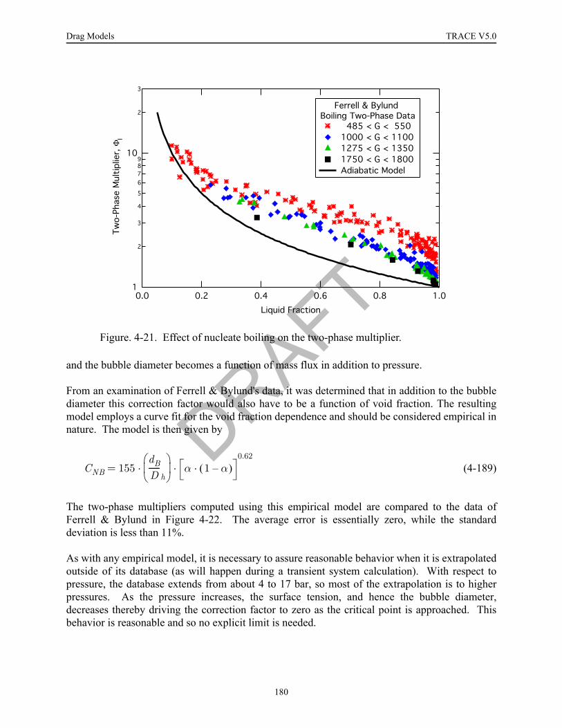
Drag Models TRACE V5.0
and the bubble diameter becomes a function of mass flux in addition to pressure.
From an examination of Ferrell & Bylund's data, it was determined that in addition to the bubblediameter this correction factor would also have to be a function of void fraction. The resultingmodel employs a curve fit for the void fraction dependence and should be considered empirical innature. The model is then given by
(4-189)
The two-phase multipliers computed using this empirical model are compared to the data ofFerrell & Bylund in Figure 4-22. The average error is essentially zero, while the standarddeviation is less than 11%.
As with any empirical model, it is necessary to assure reasonable behavior when it is extrapolatedoutside of its database (as will happen during a transient system calculation). With respect topressure, the database extends from about 4 to 17 bar, so most of the extrapolation is to higherpressures. As the pressure increases, the surface tension, and hence the bubble diameter,decreases thereby driving the correction factor to zero as the critical point is approached. Thisbehavior is reasonable and so no explicit limit is needed.
Figure. 4-21. Effect of nucleate boiling on the two-phase multiplier.
! "
#""" ! ##""
#$% ! #&"
#%" ! #""
'(
CNB 155dBD------
h⎝ ⎠⎜ ⎟⎛ ⎞
α 1 α–( )·0.62
· ·= DRAFT
180
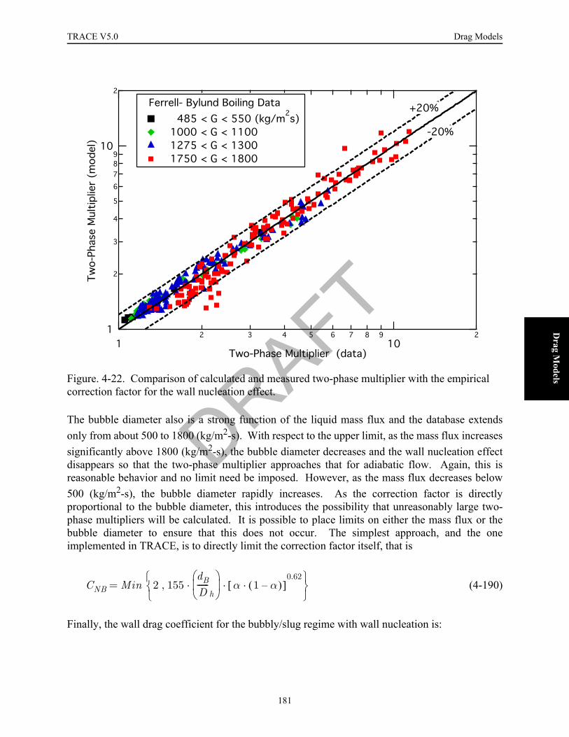
TRACE V5.0 Drag Models FOOBAR1234FOOBAR1234FOOBAR1234
Drag M
odels
The bubble diameter also is a strong function of the liquid mass flux and the database extendsonly from about 500 to 1800 (kg/m2-s). With respect to the upper limit, as the mass flux increasessignificantly above 1800 (kg/m2-s), the bubble diameter decreases and the wall nucleation effectdisappears so that the two-phase multiplier approaches that for adiabatic flow. Again, this isreasonable behavior and no limit need be imposed. However, as the mass flux decreases below500 (kg/m2-s), the bubble diameter rapidly increases. As the correction factor is directlyproportional to the bubble diameter, this introduces the possibility that unreasonably large two-phase multipliers will be calculated. It is possible to place limits on either the mass flux or thebubble diameter to ensure that this does not occur. The simplest approach, and the oneimplemented in TRACE, is to directly limit the correction factor itself, that is
(4-190)
Finally, the wall drag coefficient for the bubbly/slug regime with wall nucleation is:
Figure. 4-22. Comparison of calculated and measured two-phase multiplier with the empirical correction factor for the wall nucleation effect.
! " # " !! $%
& " # " &&
&'! " # " &(
&'! " # " &
CNB Min 2 155,dBD------
h⎝ ⎠⎜ ⎟⎛ ⎞
α 1 α–( )·[ ]0.62
· ·⎩ ⎭⎨ ⎬⎧ ⎫
=
DRAFT
181
Drag Models TRACE V5.0
(4-191)
Transition from Bubbly/Slug to Annular/Mist
For the computation of interfacial drag, the transition between the bubbly/slug and the annular/mist regimes was handled by a power-law combination. (See the counterpart section titledTransition from Bubbly/Slug to Annular/Mist in Interfacial Drag.) However, as the magnitudeof the two-phase multipliers for these regimes is similar over the entire range of liquid fractions, apower-law combination is unsuitable for the wall drag. Consequently, an explicit ramp as afunction of void fraction was introduced to provide a continuous definition of the wall dragcoefficient. Based on observations of the data used to develop the model, the model for thebubbly/slug wall drag is applied up to a void fraction of 80%, and above void fractions of 90%,the annular flow model is applied. For values of the void fraction between 80% and 90%,
(4-192)
where the bubbly/slug weighting factor is
(4-193)
This completes the description of the wall drag models for the normal pre-CHF flow regimes.The next two sections describe the models for horizontal stratified flow and for the post-CHFflow regimes respectively.
Horizontal Stratified Flow Model
In horizontal stratified flow (see Figure 4-12), both the liquid and gas phases are in contact withthe pipe wall, so the wall drag coefficient is specified for both phases. Taitel and Dukler (Ref. 4-28) gave the wall shear stresses as
(4-194)
where the friction factors are evaluated using
Cwl fwl2ρlDh------- 1 CNB+( )
2· ·=
Cwl wfBS Cwl BS,
· 1 wfBS–( ) Cwl AM,
·+=
wfBS0.9 α–0.9 0.8–---------------------
⎝ ⎠⎜ ⎟⎛ ⎞=
τwl fwl ρlVl
2
2-------------
τwg fwg ρgVg
2
2--------------
=
=
DRAFT
182

TRACE V5.0 Drag Models FOOBAR1234FOOBAR1234FOOBAR1234
Drag M
odels
(4-195)
for turbulent flow, and
(4-196)
for laminar flow. The phasic Reynolds nos. are calculated from
(4-197)
with the phasic hydraulic diameters evaluated in the manner suggested by Agrawal et. al. (Ref. 4-37):
(4-198)
Note that this definition of the phasic hydraulic diameters implies that the wall drag to the liquidis similar to that for open channel flow and that of the gas phase to closed-duct flow.
From Eq. (4-194) and considering the surface area of the wall in contact with each phase, the walldrag coefficients are:
(4-199)
As the friction factors used by Taitel and Dukler, Eq. (4-195) and Eq. (4-196), are simply thosefor a pipe, the formula of Churchill, Eq. (4-166), is used in TRACE.
The determination of whether or not the flow is stratified is made using the criteria described inStratification Criteria. Should the flow regime be in the transition region, the wall dragcoefficients are evaluated by a simple linear interpolation between the values calculated forstratified and non-stratified flow using the weighting factor given by Eq. (4-105),
fwk0.046
Re0.2k
---------------=
fwk16Rek---------=
RelρlVl Dlµl
-------------------
RegρgVgDgµg
-------------------=
=
Dl4AlSl
---------
Dg4Ag
Sg Si+( )---------------------=
=
Cwl fwlPl 2
-------Sl A-------
Cwg fwgPg 2
--------Sg A
--------·=
·=
DRAFT
183
Drag Models TRACE V5.0
(4-200)
This completes the description of the wall drag for the horizontal stratified flow regime. Thefollowing section describes the wall drag models for the inverted post-CHF flow regimes.
Post-CHF Flow Regimes
For the "inverted" post-CHF flow regimes, the wall surface temperature is beyond the Leidenfrostpoint and so only the gas phase is in contact with the wall. Consequently, wall-fluid shear onlyoccurs for the gas phase and should be zero. As described below, the inverted annularregime is treated as a direct analog to the annular regime while the dispersed flow regime istreated using a model for particle-laden flows.
Inverted Annular
The inverted annular regime is treated as a direct "inverse" analog to the annular flow regime.That is, the frictional pressure gradient is computed from
(4-201)
in terms of the two-phase multiplier for the gas phase considered to flow alone in the channel,
. The friction factor, , is the Fanning friction factor for the gas phase calculated from
the Churchill formula with
(4-202)
The wall drag coefficient is then
(4-203)
From the analogy with annular flow, the two-phase multiplier is simply
Cwk wfstrat Cwk strat,
· 1 wfstrat–( ) Cwk ns,
·+=
Cwl
dPdz-------
fΦg
22f
2Φ g,Gg Gg
Dhρg------------------------------------–=
Φg2 f
2Φ g,
Re2Φ g,
Gg Dhµg
-------------------α ρg Vg Dh
µg-------------------------------= =
Cwg Φg2
2f2Φ g,
α2ρg
Dh-----------------------------=
DRAFT
184
TRACE V5.0 Drag Models FOOBAR1234FOOBAR1234FOOBAR1234
Drag M
odels
(4-204)
and so the wall drag coefficient reduces to
(4-205)
Dispersed Flow
The frictional pressure gradient for the dispersed flow regime is calculated using an empiricalmodel for particle-laden gas flows developed by Pfeffer et. al. (Ref. 4-60). The pressure gradientis given by the formula for single-phase gas flow
(4-206)
with the gas phase friction factor replaced by the equivalent friction factor, , for a gas-particlemixture. The ratio of the friction factor for dilute suspensions was found to be a function of theloading ratio only. No significant dependence was found upon the gas Reynolds no., particlediameter, or particle density. They correlated this effective friction factor for dilute suspensionsas
(4-207)
where is the loading factor and is given by
(4-208)
For the case of dispersed flow, the loading factor becomes the ratio of the liquid to gas flow rate,so
(4-209)
The TRACE implementation of this model uses the Churchill formula for the gas friction factorand limits the loading factor to be less than 12, the maximum value in the database used todevelop the correlation. Then, the effective friction factor is
Φg2 1
α2------=
Cwg f2Φ g,
2ρgDh--------·=
dPdz-------
f
2fpg Gg GgDhρg
------------------------------–=
fpg
fpgfwg------- 1 LF+( )
0.3=
LF
LFmp
mg·-------·
=
LF1 α–( ) ρl Vl α ρg Vg
-----------------------------------=
DRAFT
185
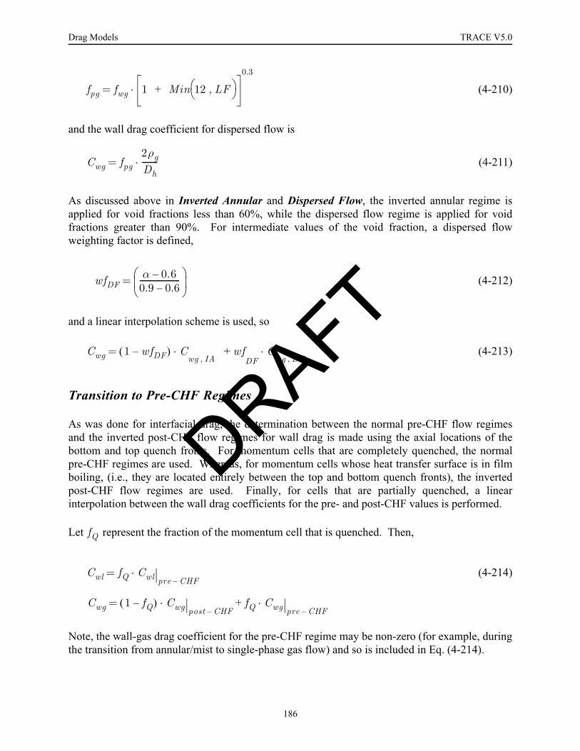
Drag Models TRACE V5.0
(4-210)
and the wall drag coefficient for dispersed flow is
(4-211)
As discussed above in Inverted Annular and Dispersed Flow, the inverted annular regime isapplied for void fractions less than 60%, while the dispersed flow regime is applied for voidfractions greater than 90%. For intermediate values of the void fraction, a dispersed flowweighting factor is defined,
(4-212)
and a linear interpolation scheme is used, so
(4-213)
Transition to Pre-CHF Regimes
As was done for interfacial drag, the determination between the normal pre-CHF flow regimesand the inverted post-CHF flow regimes for wall drag is made using the axial locations of thebottom and top quench fronts. For momentum cells that are completely quenched, the normalpre-CHF regimes are used. Whereas, for momentum cells whose heat transfer surface is in filmboiling, (i.e., they are located entirely between the top and bottom quench fronts), the invertedpost-CHF flow regimes are used. Finally, for cells that are partially quenched, a linearinterpolation between the wall drag coefficients for the pre- and post-CHF values is performed.
Let represent the fraction of the momentum cell that is quenched. Then,
(4-214)
Note, the wall-gas drag coefficient for the pre-CHF regime may be non-zero (for example, duringthe transition from annular/mist to single-phase gas flow) and so is included in Eq. (4-214).
fpg fwg 1 Min 12 LF,⎝ ⎠⎛ ⎞+·
0.3
=
Cwg fpg2ρgDh--------·=
wfDFα 0.6–0.9 0.6–---------------------
⎝ ⎠⎜ ⎟⎛ ⎞=
Cwg 1 wfDF–( ) Cwg IA ,
wf+·DF
Cwg DF,
·=
fQ
Cwl fQ Cwl pre CHF–
Cwg 1 fQ–( ) Cwg post CHF–· fQ Cwg pre CHF–
·+=
·=
DRAFT
186

TRACE V5.0 Drag Models FOOBAR1234FOOBAR1234FOOBAR1234
Drag M
odels
References4-1 N. Zuber and J. Findlay, "Average Volumetric Concentration in Two-Phase Flow
Systems," Trans. ASME J. of Heat Trans., series C, 87, 453-468 (1965).
4-2 G. B. Wallis, "One-Dimensional Two-Phase Flow," Chapter 9, McGraw-Hill, New York,NY (1969).
4-3 M. Ishii, "One-Dimensional Drift-Flux Model and Constitutive Equations for RelativeMotion Between Phases in Various Flow Regimes," Argonne National Laboratory reportANL-77-47 (1977).
4-4 I. Kataoka and M. Ishii, "Drift Flux Model for Large Diameter Pipe and New Correlationfor Pool Void Fraction," Int. J. Heat Mass Transfer, 30, 1927-1939 (1987).
4-5 M. Ishii and K. Mishima, "Two-Fluid Model and Hydrodynamic Constitutive Relations,"Nucl. Eng. and Design, 82, 107-126 (1984).
4-6 D. Bestion, "Interfacial Friction Determination for the 1-D Six Equation Two-FluidModel Used in the CATHARE Code," European Two-Phase Flow Group Meeting,Marchwood, 3-7 June 1985.
4-7 M. A. Salay, "Evaluation of Interfacial Drag Models for Use in TRAC-M Rod BundleCompoents with Validation Against Steady-State and Transient Boil-Off Experiments,"Ph.D. Thesis, Univ. of Maryland, 2001.
4-8 G. B. Wallis, "Annular Two-Phase Flow, Part 1: A Simple Theory," J. of Basic Eng., 59-72, 1970.
4-9 I. Kataoka and M. Ishii, "Prediction of Pool Void Fraction by New Drift FluxCorrelation," Argonne National Laboratory Report ANL-86-29 (NUREG/CR-4657),(1986).
4-10 R. V. Baily, P. C. Zmola, F. M. Taylor and R. J. Planchet, "Transport of Gases ThroughLiquid-Gas Mixture," paper presented at the AIChE New Orleans Meeting (1956). Takenfrom secondary reference (4-9).
4-11 P. Behringer, "Steiggeshwindigheit von Dampfblasen in Kesselrohrev," V.D.I.Forschungsheft, 365 (1934). Taken from secondary reference (4-9).
4-12 P. Coddington and R. Macian, "A Study of the Performance of Void Fraction CorrelationsUsed in the Context of Drift-Flux Two-Phase Flow Models," Nucl. Eng. Design, 215, 199-216, 2002.
DRAFT
187

Drag Models TRACE V5.0
4-13 O. Nylund, et al., "Hydrodynamic and Heat Transfer Measurements on a Full-ScaleSimulated 36-Rod Marviken Fuel Element with Uniform Heat Flux Distribution," FRIGGLoop Project, FRIGG-2, 1968.
4-14 C. Asali, T.J. Hanratty and P. Andreussi, "Interfacial Drag and Film Height for VerticalAnnular Flow," AIChE J., 31 (6), 895-902, 1985.
4-15 Andreussi and S. Zanelli, "Downward Annular and Annular-Mist Flow of Air-WaterMixtures," from Two-Phase Momentum, Heat and Mass Transfer in Chemical, Process,and Energy Engineering Systems, Volume 1, Hemisphere Publishing, 1978.
4-16 M. Ishii and K. Mishima, "Droplet Entrainment Correlation in Annular Two-Phase Flow,"Int. J. Heat Mass Transf., 32(10),1835-1845, 1989.
4-17 M. Ishii and M. A. Grolmes, "Inception Criteria for Droplet Entrainment in Two-PhaseConcurrent Film Flow," AIChE Journal, 21 (2), 308-318, 1975.
4-18 G. B. Wallis, letter to the editor on "Phenomena of Liquid Transfer in Two-PhaseDispersed Annular Flow," Int. J. Heat Mass Transfer, 11, 783-785, 1968.
4-19 I. I. Paleev and B. S. Filippovich, "Phenomena of Liquid Transfer in Two-Phase DispersedAnnular Flow," Int. J. Heat Mass Transfer, 9, 1089-1093, 1966.
4-20 D. A. Steen, M. S. Thesis, Dartmouth College, 1964.
4-21 G. B. Wallis, "The Onset of Droplet Entrainment in Annular Gas-Liquid Flow," Report no.62GL127, General Electric Co., Schenectady, N.Y., 1962.
4-22 D. A. Steen and G. B. Wallis, "The Transition from Annular to Annular-Mist ConcurrentTwo-Phase Down Flow," AEC Report NYO-3114-2, 1964.
4-23 M. Ishii and T.C. Chawla, "Local Drag Laws in Dispersed Two-Phase Flow," ArgonneNational Laboratory Report ANL-79-105 (NUREG/CR-1230), December 1979.
4-24 I. Kataoka, M. Ishii, and K. Mishima, "Generation and Size Distribution of Droplets inAnnular Two-Phase Flow," Transactions of the ASME, 105, 230-238, June 1983.
4-25 R. A. Mugele and H. D. Evans, "Droplet Size Distribution in Sprays," Ind. Eng. Chem.,43, p. 1317, 1951.
4-26 M. W. Cappiello, "A Model for the Interfacial Shear in Vertical, Adiabatic, Annular-MistFlow," Los Alamos National Laboratory Report, LA-CP-89-392, October 1989.
4-27 D. Barnea, "A Unified Model for Predicting Flow-Pattern Transitions for the WholeRange of Pipe Inclinations," Int. J. Multiphase Flow, 13 (1), 1-12, 1987.
DRAFT
188

TRACE V5.0 Drag Models FOOBAR1234FOOBAR1234FOOBAR1234
Drag M
odels
4-28 Y. Taitel and A.E. Dukler, "A Model for Predicting Flow Regime Transitions in HorizontalAnd Near Horizontal Gas-Liquid Flow," AIChE Journal, 22 (1), 47-55, 1976.
4-29 H. Nakamura, "Slug Flow Transition in Horizontal Gas/Liquid Two-Phase Flows," JapanAtomic Energy Research Institute Report, JAERI-Research 96-022, May 1996.
4-30 Y. Anoda et. al., "Flow Regime Transition in High-Pressure Large-Diameter HorizontalTwo-Phase Flow," 26th ASME/AIChE/ANS National Heat Transfer Conference,Philadelphia, 1989.
4-31 W.G. Choe, L. Weinberg and J. Weisman, "Observation and Correlation of Flow PatternTransition in Horizontal, Co-Current Gas-Liquid Flow," in Two-Phase Transport andReactor Safety (Edited by T.N. Veziroglu & S. Kakac), Hemisphere, Washington, 1978.
4-32 J.W. Spore et. al., "TRAC-PF1/Mod2: Volume I. Theory Manual," NUREG/CR-5673,1993.
4-33 H.J. Richter et. al., "De-entrainment and Counter-Current Air-Water Flow in a ModelPWR Hot Leg," NRC-0193-9, 1978.
4-34 MPR Associates, Inc., "Summary of Results from the UPTF Hot Leg Separate EffectsTest, Comparison to Scaled Tests and Application to U.S. Pressurized Water Reactors,"MPR Report MPR-1024, September 1987.
4-35 A. Ohnuki, H. Adachi and Y. Murao, "Scale Effects on Countercurrent Gas-Liquid Flowin Horizontal Tube Connected to Inclined Riser," ANS National Heat TransferConference, Pittsburgh, Pennsylvania, pp. 40-49, 1987.
4-36 S.W. Churchill, "Friction Factor Equations Spans All Fluid-Flow Regimes," ChemicalEng., November, 91-92, 1977.
4-37 S.S. Agrawal, G.A. Gregory and G.W. Govier, "An Analysis of Horizontal Stratified Two-Phase Flow in Pipes," Can. J. Chem. Eng., 51, 280-286, 1973.
4-38 F. de Cachard, "Development, Implementation, and Assessment of Specific Closure lawsfor Inverted-Annular Film-Boiling in a Two-Fluid Model," USNRC InternationalAgreement Report, NUREG/IA-0133, 1996.
4-39 N. Andritsos and T.J. Hanratty, "Influence of Interfacial Waves in Stratified Gas-LiquidFlows," AIChE Journal, 33 (3), 444-454, 1987.
4-40 M. Kawaji and S. Banerjee, "Application of a Multifield Model to Reflooding of a HotVertical Tube: Part II - Analysis of Experimental Results," J. of Heat Transfer, 110, 710-720, 1988.
DRAFT
189

Drag Models TRACE V5.0
4-41 R. Clift, J.R. Grace and M.E. Weber, Bubbles, Drops, and Particles, Chapter 7, p. 179,Equation [7-14], Academic Press, New York, 1978.
4-42 J.F Richardson and W.N. Zaki, "Sedimentation and Fluidisation, Part 1," Trans. Instn.Chem. Engrs., 32, 35-53, 1954.
4-43 G.B. Wallis, "The Terminal Speed of Single Drops or Bubbles in an Infinite Medium," Int.J. Multiphase Flow, 1, 491-511, 1974.
4-44 J. Kitscha and G. Kocamustafaogullari, "Breakup Criteria for Fluid Particles," Int. J.Multiphase Flow, 15 (4), 573-588, 1989.
4-45 K.H. Ardron and P.C. Hall, "Droplet Hydrodynamics in the Dispersed Flow Regime inBottom Flooding," in Transient Two-Phase Flow: Proceedings of the Third CSNISpecialist Meeting, edited by M.S. Plesset, N. Zuber, and I. Catton, HemispherePublishing Corp., pp. 205-225, 1983.
4-46 R. Clift, J.R. Grace and M.E. Weber, Bubbles, Drops, and Particles, Chapter 5, p. 111,Table 5.1, Academic Press, New York, 1978.
4-47 M. Rensizbulut and M.C. Yuen, "Numerical Study of Droplet Evaporation in a High-Temperature Stream," J. of Heat Transfer, 105, 389-397, 1983.
4-48 I. Kataoka and M. Ishii, "Mechanistic Modeling of Pool Entrainment Phenomenon," Int. J.of Heat Mass Transfer, 27 (11), 1999-2014, 1984.
4-49 M.A.Ebadian and Z.F. Dong, "Forced Convection, Internal Flow in Ducts," Chapter 5 ofthe Handbook of Heat Transfer, edited by W.M. Rohsenow, J.P. Hartnett and Y.I. Cho, 3rdedition, McGraw Hill, 1998.
4-50 G.B. Wallis, One-Dimensional Two-Phase Flow, Chapter 11, pp. 323-329, McGraw-Hill,New York, 1969.
4-51 G.F. Hewitt and N.S. Hall-Taylor, Annular Two-Phase Flow, Chapter 5, p. 79, Equation[5.4], Pergamon Press, Oxford, 1970.
4-52 S.E. Haaland, "Simple and Explicit Formulas for the Friction Factor in Turbulent PipeFlow," J. Fluids Eng., 105, 89-90, 1983.
4-53 R.W. Lockhart and R.C. Martinelli, "Proposed Correlation of Data for Isothermal Two-Phase, Two-Component Flow in Pipes," Chem. Eng. Prog., 45 (1), 39-48, 1949.
4-54 J.K. Ferrell and D.M. Bylund, "A Study of Convection Boiling Inside Channels," FinalReport, Volume II, North Carolina State University, Dept. of Chemical Eng., June 1966.
DRAFT
190

TRACE V5.0 Drag Models FOOBAR1234FOOBAR1234FOOBAR1234
Drag M
odels
4-55 Y. Yamazaki and M. Shiba, "A Comparative Study on the Pressure Drop of Air-Water andSteam-Water Flows," in Cocurrent Gas-Liquid Flow, Proceedings of an InternationalSymposium on Research in Cocurrent Gas-Liquid Flow at the University of Waterloo, pp.359-380, Plenum Press, New York, 1969.
4-56 Y. Yamazaki and K. Yamaguchi, "Characteristics of Cocurrent Two-Phase Downflow inTubes," J. Nuclear Science and Technolgy, 16 (4), 245-255, 1979.
4-57 J.K. Ferrell and J.W. McGee, "A Study of Convection Boiling Inside Channels," FinalReport, Volume III, North Carolina State University, Dept. of Chemical Eng., June 1966.
4-58 J.G. Collier, Convective Boiling and Condensation, Chapter 6, pp. 186-188, McGraw-Hill,London, 1972.
4-59 S. Levy, "Forced Convection Subcooled Boiling Prediction of Vapor VolumetricFraction," Int. J. Heat Mass Transfer, 10, 951-965, 1967.
4-60 R. Pfeffer, S. Rossetti and S. Lieblein, "Analysis and Correlation of Heat TransferCoefficients and Friction Factor Data for Dilute Gas-Solid Suspensions," NASA TN D-3603, September 1966.
4-61 G. F. Hewitt, R. D. King and P. C. Lovegrove, "Techniques for Liquid Film and PressureDrop Studies in Annular Two-Phase Flow," AERE-R3921, United Kingdom AtomicEnergy Authority, Harwell, England, 1962.
4-62 L. E. Gill and G. F. Hewitt, "Further Data on the Upwards Annular Flow of Air-WaterMixtures," AERE-R3935, United Kingdom Atomic Energy Authority, Harwell, England,1962.
4-63 L. E. Gill, G. F. Hewitt and D. N. Roberts, "Studies of the Behaviour of DisturbanceWaves in Annular Flow in a Long Vertical Tube," AERE-R6012, United Kingdom AtomicEnergy Authority, Harwell, England, 1969.
4-64 P. B. Whalley, G. F. Hewitt and P. Hutchinson, "Experimental Wave and EntrainmentMeasurements in Vertical Annular Two-Phase Flow," AERE-R7521, United KingdomAtomic Energy Authority, Harwell, England, 1973.
DRAFT
191

Drag Models TRACE V5.0
DRAFT
192

FOOBAR1234FOOBAR1234FOOBAR1234FOOBAR1234
Interfacial H
eat Transfer
Models
5 Interfacial Heat Transfer
ModelsFOOBAR1234FOOBAR1234FOOBAR1234FOOBAR1234FOOBAR1234
This chapter describes the TRACE interfacial heat transfer package.
Nomenclature = minor radius of prolate ellipsoid
= flow area (m2)
= flow area of phase in stratified flow (m2)
= interfacial (m2)
= interfacial area per unit volume (m-1)
= major radius of prolate ellipsoid or the mass transfer driving potential
= "blowing factor" for effect of mass transfer upon heat transfer
= specific heat (J/kg-K)
= concentration (kg/m3)
= coefficient in formula for bubbly/slug interfacial area, see Eq. (5-29)
= particle diameter, either bubble or drop, (m).
= pipe diameter (m)
= hydraulic diameter (m)
= diameter used in bubbly/slug flow regime, see Eq. (5-30)
= diffusion coefficient (m2/s)
a
A
Ak k
Ai
Ai′′′
b
Bf
cp
C
C∗
d
D
Dh
D∗
D0
DRAFT
193

Interfacial Heat Transfer Models TRACE V5.0
= ellipticity, see Eq. (5-96)
= entrainment fraction
= "fog factor" to account for increase of sensible heat transfer due to mist
formation
= fraction of a cell that is quenched, i.e., in the pre-CHF flow regime.
= fraction of the surface covered by a liquid film
= gravitational acceleration (m/s2)
= mass flux (kg/m2-s)
= Grashof no.,
= heat transfer coefficient (W/m2-K)
= interfacial heat transfer coefficient for phase to interface (W/m2-K)
= latent heat of evaporation (J/kg)
= enthalpy of phase (J/kg)
= mass transfer coefficient (m/s)
= empirical constant in Eq. (5-38)
= thermal conductivity (W/m-K)
= Laplace no., equal to
= molecular weight (kg/mole)
= viscosity no. for phase ,
= Nusselt no.,
= pressure (Pa)
= partial pressure of the non-condensable gas in the gas-vapor mixture (Pa)
= vapor partial pressure of gas-vapor mixture (Pa)
= pitch-to-diameter ratio for a rod bundle
= Peclet no.,
= Prandtl no.,
e
E
ffog
fQ
fwet
g
G
Gr L3 g ρ∆· ·( ) ρ V2·( )⁄=[ ]
h
hki k
hfg
hk k
hM
H0
k
La σ g ρ∆⁄
MW
Nµk k Nµk µk ρkσLa( )1 2⁄
⁄=
Nu h d· k⁄=( )
P
PNC
Pv
P Dr⁄
Pe Re Pr·=( )
Pr cp µ k⁄=( )
DRAFT
194

TRACE V5.0 Interfacial Heat Transfer Models FOOBAR1234FOOBAR1234FOOBAR1234FOOBAR1234
Interfacial H
eat Transfer
Models
= interfacial heat flux from phase k to the interface (W/m2)
= interfacial heat transfer rate per unit volume from phase (W/m3)
= gas constant for steam (J/kg-K)
= Reynolds no.
= surface area (m2)
= width of gas-liquid interface in stratified flow
= Schmidt no.,
= Sherwood no.,
= temperature (K)
= saturation temperature at the total pressure (K)
= saturation temperature at the bulk vapor partial pressure (K)
= velocity (m/s)
= relative velocity (m/s)
= terminal velocity in infinite medium (m/s)
= maximum dimensionless circulation velocity at drop surface
= weighting factor
= vapor mass fraction in gas-vapor mixture
Greek = void fraction (volume fraction of gas phase )
= volume fraction of phase
= film thickness (m)
= density difference between liquid and gas phases (kg/m3)
= density (kg/m3)
= mass transfer rate per unit volume, negative for condensation, positive for
evaporation (kg/m3-s)
= liquid film flow rate per unit wetted perimeter (kg/s-m)
= mass transfer rate per unit volume due to interfacial heat transfer
qki″
qki′′′ k
Rs
Re
S
Si
Sc ν D0⁄=( )
Sh hM d· D0⁄=( )
T
Tsat
Tsv
V
Vr
V∞
V∗max
wf
xv
α αg
αk k
δ
ρ∆
ρ
Γ
Γf
Γi
DRAFT
195

Interfacial Heat Transfer Models TRACE V5.0
= mass transfer rate per unit volume due to subcooled boiling
= mass flux at interface due to condensation or evaporation (kg/m2-s)
= condensation mass flux calculated without variable property correction (kg/
m2-s)
= turbulent length scale
= viscosity (Ns/m2)
= dynamic viscosity (m/s2),
= surface tension (N/m)
Subscripts = air
= annular/mist flow regime
= bubble
= condensation or the core region in annular/mist or inverted annular flow
= condensation
= critical value
= drop
= dispersed-bubble
= dispersed flow regime
= drop
= evaporation
= film
= the liquid film or a value at a reference "film" temperature
= flashing
= forced convection
= gas-to-liquid
= evaluated using Gnielinski correlation for turbulent forced convection
= vapor-gas mixture
= interface
= inverted annular
= inverted slug
Γsub
Γ″
Γ″0
λt
µ
ν ν µ ρ⁄=
σ
a
AM
b
c
cond
crit
d
DB
DF
drop
evap
f
film
flash
FC
gl
Gnielinski
g
i
IA
IS
DRAFT
196

TRACE V5.0 Interfacial Heat Transfer Models FOOBAR1234FOOBAR1234FOOBAR1234FOOBAR1234
Interfacial H
eat Transfer
Models
= phase index, = liquid, and = gas/vapor mixture
= liquid
= laminar
= liquid-to-interface
= large bubble (e.g., slug or Taylor cap bubbles)
= non-stratified
= non-condensable or natural convection
= component due to thermal radiation
= value from Rayleigh-Taylor instability
= steam
= value at saturation
= sensible heat component
= stratified
= subcooled or subcooled boiling
= superheat
= saturation at the vapor partial pressure
= subcooled boiling
= turbulent
= terminal
= turbulent
= vapor
= vapor-to-interface
= based on equivalent volume
= wall
IntroductionInterfacial heat transfer models are required for closure of both the mass and energy equations. InTRACE, the interfacial mass transfer rate per unit volume, , is defined as the sum of the masstransfer rates from interfacial heat transfer and from subcooled boiling, as
k l g
l
lam
li
LB
ns
NC
rad
R T–
s
sat
sens
strat
sub
sup
sv
SB
t
term
turb
v
vi
V
w
Γ
DRAFT
197

Interfacial Heat Transfer Models TRACE V5.0
(5-1)
where is the mass transfer rate per unit volume due to interfacial heat transfer, and is themass transfer rate per unit volume due to subcooled boiling.
The mass transfer rate due to subcooled boiling will be described in Chapter 6, SubcooledBoiling Model. The mass transfer rate caused by interfacial heat transfer is evaluated from thethermal energy jump relation
(5-2)
where and are the interfacial heat transfer rates per unit volume for the liquid-to-interface and vapor-to-interface respectively. The denominator of Eq. (5-2) is not simply thelatent heat, , but rather is given by
(5-3)
where the second subscript "sat" denotes that the phase enthalpy is evaluated at saturation. Thisformulation correctly accounts for the sensible heat that is first required to bring the disappearingphase to saturation and that the generated phase appears at saturation.
In the TRACE numerical scheme, the liquid-gas interface is assumed to be at the saturationtemperature corresponding to the bulk vapor partial pressure for the mass-energy computationalcell. This temperature is denoted by where
(5-4)
and is distinct from the saturation temperature, , computed from the total pressure,
(5-5)
that is especially important for wall heat transfer processes such as nucleate boiling.
The interfacial heat transfer rates are then given by
Γ Γi Γsub+=
Γi Γsub
Γiq'''li q'''vi+hv∗ hl∗–( )
--------------------------=
q'''li q'''vi
hfg
h∗v hl∗–( )h
v sat,hl–( ) ; Γ 0>
hv hl sat,
–( ) ; Γ 0<⎩⎪⎪⎨⎪⎪⎧
=
Tsv
Tsv Tsat Pv( )=
Tsat
Tsat Tsat P( )=
DRAFT
198

TRACE V5.0 Interfacial Heat Transfer Models FOOBAR1234FOOBAR1234FOOBAR1234FOOBAR1234
Interfacial H
eat Transfer
Models
(5-6)
for the liquid-side heat transfer and by
(5-7)
for the gas-side heat transfer. For the special case where the liquid is superheated with respect tosaturation at the total pressure, , rapid nucleation will occur at any surface and theresulting interfacial heat transfer coefficient will increase dramatically as the level of liquidsuperheat increases. Under these conditions, Eq. (5-6) is modified to add an additional term forflashing, that is,
(5-8)
When non-condensable gases are present, several modifications are made to the above equations.First, as discussed below in Default Model for Condensation, the additional heat transferresistance associated with the diffusion of the non-condensable gas either to or from the interfaceis added to that for the liquid-side heat transfer. Thus, Eq. (5-6) becomes
(5-9)
where the second subscript "NC" indicates that the non-condensable gas effect has been added.
Second, for the effect of non-condensable gases upon the gas-side heat transfer, the interfacialheat transfer coefficient determined using the models described below is multiplied by the relativepartial pressure in the energy equation. Thus,
(5-10)
which forces the vapor-interface heat transfer to zero as the vapor is depleted. Finally, allowanceis made for the sensible heat transfer between the gas mixture and the liquid phase. The gas-liquid heat transfer coefficients described below are similarly multiplied by the relative partialpressure of the non-condensable gas, so that
(5-11)
and the sensible heat transfer goes to zero as pure-steam conditions are approached.
q′′′li hli A′′′i Tl Tsv–( )· ·=
q′′′vi hvi A′′′i Tg Tsv–( )· ·=
Tl Tsat>
q′′′li hli Ai′′′ Tl Tsv–( ) hflash Ai′′′ Tl Tsat–( )· ·+· ·=
qli′′′ hli NC,
Ai′′′ Tl Tsv–( )· ·=
qvi″PvP------ hvi Tg Tsv–( )· ·=
qgl″PNCP
----------- hgl Tg Tl–( )· ·=
DRAFT
199

Interfacial Heat Transfer Models TRACE V5.0
Therefore, models need to be specified for the four heat transfer coefficients, , , , and
, and the associated interfacial area. These interfacial heat transfer coefficients are dependentupon the flow regime selected by the code. As explained above for the interfacial drag coefficient,TRACE considers three distinct classes of flow regimes:
•Pre-CHF: these consist of the bubbly/slug and the annular/mist regimes as explained in Chapter 4, Pre-CHF Interfacial Drag Models.
•Stratified: the horizontal stratified flow regime is available for 1-D components that are either horizontal or inclined as explained in Chapter 4, Stratified Flow Interfacial Drag Models.
•Post-CHF: this encompasses the "inverted" flow regimes that occur when the wall is too hot for liquid-wall contact, see Chapter 4, Post-CHF Interfacial Drag Models.
The interfacial heat transfer models used by TRACE for these flow regimes are detailed below inPre-CHF Interfacial Heat Transfer Models, Stratified Flow Interfacial Heat Transfer Modelsand Post-CHF Interfacial Heat Transfer Models. In addition, a special section is added todescribe the models for the effect on non-condensable gases upon condensation and evaporation.
Pre-CHF Interfacial Heat Transfer ModelsIn TRACE, as discussed previously for the evaluation of the interfacial drag coefficient, fourprincipal flow regimes are considered for vertical flow as depicted in Figure 4-1 The three"bubbly" flow regimes, i.e., dispersed bubble, slug flow and Taylor cap bubble, are collectivelyreferred to as the "bubbly/slug" flow regime. The models used for the interfacial heat transfer inthe bubbly/slug and annular/mist flow regimes are applied to both vertical and horizontalgeometries. However, for the horizontal case, a special horizontal stratification model isintroduced as described in Stratified Flow Interfacial Heat Transfer Models below.
The pre-CHF flow regime map used for interfacial heat transfer is that of TRAC-PF1/MOD2, asdepicted in Figure 5-1. The flow regime determination is primarily based on void fraction withthe mass flux range for the Taylor cap or slug bubble flow regime limited. Both the region overwhich a flow regime is applied and the corresponding models for interfacial area and heat transfercoefficient are detailed below. Also, the churn regime, that is, the transition regime between thebubbly/slug and the annular/mist flow regimes, where the nature of the two-phase interface is notclearly defined, is approximated by interpolation between the values for the other regimes.
Bubbly Flow Regime
The upper limit of the void fraction for the dispersed bubble flow regime is nominally given avalue of 30%. This value was chosen as it roughly corresponds to bubble concentrations wherecoalescence rates rapidly drive the regime towards either Taylor cap or slug flow. For high liquidflow rates, however, liquid phase turbulence can break-up the gas phase into small, dispersed
hli hvi hflash
hgl
DRAFT
200

TRACE V5.0 Interfacial Heat Transfer Models FOOBAR1234FOOBAR1234FOOBAR1234FOOBAR1234
Interfacial H
eat Transfer
Models
bubbles. Choe et. al. (Ref. 4-31) give the criterion for this transition to homogeneous dispersedbubbly flow as a simple mass flux limit, specifically, that homogeneous flow exists for massfluxes greater than about 2700 kg/m2-s.
In TRACE, the Choe-Weisman mass flux criterion for the transition to dispersed bubble flow isimplemented by a linear ramp on the maximum allowable volume fraction for the dispersedbubbles. That is,
(5-12)
The diameter of the dispersed bubbles is approximated by that for a distorted bubble and is afunction of the Laplace coefficient, namely
(5-13)
Figure. 5-1. Pre-CHF flow regime map for interfacial heat transfer.
αDB
0.3 ; G 2000 kg m2s⁄( )≤
0.3 0.2 G 2000–2700 2000–------------------------------⎝ ⎠
⎛ ⎞·+ ; 2000 G 2700 kg m2s⁄( )< <
0.5 ; G 2700 kg m2s⁄( )≥⎩⎪⎪⎪⎨⎪⎪⎪⎧
=
dDB 2 La· 2 σ g∆ρ⁄·= =
DRAFT
201

Interfacial Heat Transfer Models TRACE V5.0
and is constrained to be in the range
(5-14)
If the void fraction is less than , the interfacial area for the dispersed bubbles is simply
(5-15)
However, for larger values of the void fraction, a combination of small dispersed bubbles andlarge slug or cap bubbles is assumed to exist. For this case, Ishii and Mishima (Ref. 5-1) give theinterfacial area concentration due to small bubbles as a function of the average void fractionwithin the liquid slug, so that
(5-16)
The interfacial area and heat transfer associated with the large slug or cap bubbles is described inthe following section. It remains to calculate the interfacial heat transfer coefficient for thedispersed bubbles as it is the product, , that is needed for the energy equation.
For both evaporation and condensation, the heat transfer between the liquid and the bubbleinterface is modeled using the Ranz-Marshall correlation (Ref. 5-2) as recommended by Warrieret. al. (Ref. 5-3). The heat transfer coefficient is then
(5-17)
where the Nusselt no. is given by
(5-18)
For high bubble Reynolds no. conditions, the values of the Nusselt no. given by the Ranz-Marshall correlation are similar but somewhat lower than those of the Chen-Mayinger correlation(Ref. 5-4) that was used in TRAC-PF1/MOD2. However, for low Reynolds no. conditions, thebehavior of the Ranz-Marshall correlation is clearly superior as it correctly reduces to the steadystate conduction solution for a sphere immersed in an infinite fluid (Ref. 5-5).
The bubble Reynolds no. used in Eq. (5-18) is a function of the dispersed bubble relative velocityand is defined
1.0 10 4–× m( ) dDB 0.9 Dh·≤ ≤
αDB
A′′′i DB,
6 α·dDB-----------=
A′′′i DB,
6 αDB·dDB
------------------ 1 α–1 αDB–-------------------⎝ ⎠
⎛ ⎞·=
hAi
hli DB,
kldDB---------- NuDB·=
NuDB 2.0 0.6 ReDB1 2⁄
Prl1 3⁄
··+=
DRAFT
202
TRACE V5.0 Interfacial Heat Transfer Models FOOBAR1234FOOBAR1234FOOBAR1234FOOBAR1234
Interfacial H
eat Transfer
Models
(5-19)
In practice, the dispersed bubble relative velocity cannot simply be assumed to be given by thephasic relative velocity, , that results from the solution of the two-fluid momentumequations. This is because the gas field in TRACE can represent a combination of large and smallbubbles, and so
is generally true. To get a more accurate estimate of the dispersed bubble relative velocity, thebubble terminal velocity is used as an upper limit. Thus,
(5-20)
where the dispersed bubble terminal velocity is calculated for a distorted particle with the multi-particle correction of Richardson & Zaki (Ref. 4-42). For a single distorted particle, Wallis'formula (Ref. 4-43) gives
(5-21)
and, applying the Richardson-Zaki correction, the multi-particle terminal velocity is
(5-22)
Note – The exponent in Eq. (5-22) is incorrect in TRACE V5.0. It should be 1.39. This will be corrected in a follow-on bug fix release.
Normally, due both to its high values of heat transfer coefficient and interfacial area, the dispersedbubble component of the interfacial heat transfer dominates over that of the Taylor cap/slugbubble described below.
Eq. (5-18) gives the formula for the Nusselt no. for the liquid-side interfacial heat transfer. Tocomplete the description, models are also needed for the gas-side heat transfer and, when non-condensable gases are present, for the sensible heat transfer between the gas and the liquid. In
ReDB
ρl Vr DB,
dDB· ·
µl----------------------------------------=
Vg Vl–
Vr DB,
Vg Vl–
Vr DB,
Min Vg Vl– VDB term,
,=
Vr ∞,
2σ g ∆ρ· ·
ρl2
-----------------------⎝ ⎠⎜ ⎟⎛ ⎞ 1 4⁄
=
VDB term,
Vr ∞,
1 α–( )2.39·= DRAFT
203

Interfacial Heat Transfer Models TRACE V5.0
TRACE, these heat transfer coefficients are simply set to the constant values that were usedpreviously in TRAC-PF1/MOD2. That is,
(5-23)
The vapor-interface heat transfer coefficient, , is seldom important in governing the masstransfer rate for bubbly flow and it is thought adequate to keep it at a constant value that issufficiently high enough to prevent large departures from thermal equilibrium. For the sensibleheat transfer when non-condensable gases are present, however, this argument does not hold.This is especially true as using Eq. (5-23) for ignores the heat transfer resistance on theliquid-side. A future update to TRACE 5.0 will correct this oversight.
When subcooled boiling is present, the liquid-side interfacial heat transfer for bubbly flow ismodified to account for near-wall condensation. The TRACE model for this is described below inModifications for Subcooled Boiling. The following section describes the models for the largebubbles that occur in the cap bubble/slug flow regimes.
Cap Bubble/Slug Flow Regime
For void fractions greater than the dispersed bubble limit, , but less than 50%, the flowregime for interfacial heat transfer is considered to be either cap bubble or slug flow. In eithercase, the bubble diameter is much larger than for the dispersed bubbly regime, so that both theinterfacial area and heat transfer coefficient are much smaller. Consequently, the component ofthe interfacial heat transfer due to these large bubbles is dwarfed by that of the smaller dispersedbubbles contained within the liquid slugs. Nevertheless, for completeness, the large bubblecomponent is calculated and added to that of the dispersed bubbles, so that
(5-24)
The approach taken to describe the interfacial heat transfer for cap and slug bubbles is similar tothat used above for dispersed bubbles with the primary differences being the estimation of thebubble diameter, the interfacial area, and the limiting value of the relative velocity. To estimatethe interfacial area, the first step is to determine whether the flow regime is cap bubble or slugflow. Kataoka and Ishii (Ref. 4-4) state that slug bubbles cannot be sustained for channels with adiameter much larger than . Similarly, the interface stability analysis of Kitscha andKocamustafaogullari (Ref. 4-44) yields
(5-25)
hvi hgl 1000 W m2K⁄( )= =
hvi
hgl
αDB
hli Ai·( ) hli Ai·( )DB hli Ai·( )LB+=
40La
db V,
27.07 1 Nµl+( )0.83
La·=
DRAFT
204

TRACE V5.0 Interfacial Heat Transfer Models FOOBAR1234FOOBAR1234FOOBAR1234FOOBAR1234
Interfacial H
eat Transfer
Models
for the maximum stable bubble diameter, where is the volume equivalent diameter. For
water, the liquid viscosity number is much less than unity and so,
(5-26)
Using the geometry of an idealized cap bubble with a wake angle of 55o, the diameter of the baseof a cap bubble would then be about . Further, assuming that a cap bubble will grow into aslug bubble when its diameter reaches about , the channel critical diameter for thetransition to slug flow is then
(5-27)
So, for channels having a hydraulic diameter less than , large bubbles will be treated as
slugs, while for larger diameter channels they will be Taylor cap bubbles.
For the cap bubble/slug regime, the interfacial area associated with the large bubbles is computedusing the formula of Ishii and Mishima (Ref. 5-1), specifically
(5-28)
where the values of the coefficient C* and the diameter D* depend on whether or not the flowregime is slug or cap bubble and is a function of the channel hydraulic diameter. Namely,
(5-29)
and
(5-30)
The liquid-side heat transfer coefficient for these large bubbles is
db V,
db V,
27 La·≈
45La0.9Dh
Dh crit,
50 La·≈
Dh crit,
Ai LB,′′′ C∗
D∗-------
α αDB–1 αDB–--------------------
⎝ ⎠⎜ ⎟⎛ ⎞
·=
C∗4.5 ; Dh D
h crit,<
16 ; Dh Dh crit,
≥⎩⎪⎪⎨⎪⎪⎧
=
D∗Dh ; Dh D
h crit,<
Dh crit,
; Dh Dh crit,
≥⎩⎪⎪⎨⎪⎪⎧
=
DRAFT
205

Interfacial Heat Transfer Models TRACE V5.0
(5-31)
where the Nusselt no. is computed using the Ranz-Marshall correlation Eq. (5-18) and the bubbleReynolds no. is
(5-32)
As was the case for small dispersed bubbles, the relative velocity for the large bubbles cannotsimply be taken to be the phasic velocity difference, . Thus,
(5-33)
An upper limit on the relative velocity for cap and slug bubbles is estimated using the formulasfrom Wallis (Ref. 4-43) for the terminal velocity of his "region 5" bubbles with the correctionfactor for tube radius. Define the non-dimensional bubble diameter as
(5-34)
and a relative velocity in an infinite medium by
(5-35)
Then, the limiting value of the relative velocity is
(5-36)
This completes the description for the liquid-side interfacial heat transfer for the large bubbles inthe cap bubble/slug flow regimes. For both the gas-side, , and sensible heat transfer, , theconstant values used for the dispersed bubbles are retained. The small bubble interfacial area issimply augmented by that for the large bubbles, e.g.,
hli LB,
kl
D∗------- NuLB·=
ReLB
ρl Vr LB,
D∗· ·
µl-------------------------------------=
Vg Vl–
Vr LB,
Min Vg Vl– VLB term,
,⎩ ⎭⎨ ⎬⎧ ⎫
=
d∗LBD∗Dh-------=
Vr ∞,
22
-------g ∆ρ D∗··
ρl--------------------------------·=
VLB term,
Vr ∞,
; d∗LB 0.125<
1.13 Vr ∞,
e d∗LB–· · ; 0.125 d∗LB 0.6< <
0.496 Vr ∞,
d∗LB⁄· ; d∗LB 0.6≥⎩⎪⎪⎪⎨⎪⎪⎪⎧
=
hvi hgl
DRAFT
206

TRACE V5.0 Interfacial Heat Transfer Models FOOBAR1234FOOBAR1234FOOBAR1234FOOBAR1234
Interfacial H
eat Transfer
Models
(5-37)
Modifications for Subcooled Boiling
When subcooled boiling is present, the liquid-side interfacial heat transfer for bubbly flow ismodified to account for near-wall condensation. For this effect, TRACE uses the modelsuggested by Lahey and Moody (see Eq. 5.174 in Reference 5-6), which is given by
(5-38)
where H0 is an empirical constant and is the interfacial heat flux due to near-wallcondensation. The product of the interfacial heat transfer coefficient and interfacial areaconcentration for subcooled boiling is then
(5-39)
Lahey and Moody suggest that
(5-40)
and this is the value used in TRACE. Also, to provide a reasonable value as the void fractionapproaches zero, Eq. (5-39) is rewritten as
(5-41)
This model is applied only when subcooled boiling is occurring, that is
and
.
Finally, as the condition of bulk boiling is approached, a smooth transition between the subcooledboiling model and that for normal bubbly flow is necessary. This is accomplished by using asimple void fraction ramp between values of 10% and 20%. The subcooled boiling weightingfactor is defined
hvi Ai·( ) hvi Ai DB,
Ai LB,
+( )·=
qcond″ H0
Dh4
------- hfgρlρg∆ρ---------- α Tl Tsv–( )· · · · ·=
qcond″
hliAi′′′( )SB H0 hfg
ρlρg∆ρ---------- α· · ·=
H0 0.075 s K–( ) 1–=
hliAi′′′( )SB 0.075 hfg
ρlρg∆ρ---------- Max 0.0001 α,[ ]· · ·=
Γsub 0>
Tl Tsv<
DRAFT
207

Interfacial Heat Transfer Models TRACE V5.0
(5-42)
and the interfacial heat transfer for bubbly flow is given by
(5-43)
Interfacial Heat Transfer Models for the Annular/Mist Flow Regime
For void fractions in excess of 75%, the flow regime for interfacial heat transfer is assumed to beannular/mist. As was the case for the computation of interfacial drag, components for both anannular film and entrained droplets are calculated separately and then combined. For example,
(5-44)
The models used for annular films are discussed first, followed by those for the entraineddroplets.
Annular Film Models
For annular films, the most important quantity is the film thickness as it is the characteristic lengthfor heat transfer. In TRACE, this characteristic length results directly from the solution of thetwo-fluid momentum equations that yield the void fraction as a function of wall drag, interfacialshear, and gravity. The film thickness is then calculated from the void fraction based on thegeometry. For most components, the film thickness is computed using the formula for tubegeometry, that is,
(5-45)
A special case is made for the downcomer region of the 3-D vessel component, here the filmthickness is computed assuming the geometry of an annulus. So,
(5-46)
In both cases, the film thickness is constrained to be greater than 10 . This value was selectedas a limiting value because a film with that thickness gives a heat transfer coefficient of about thesame magnitude as dropwise condensation.
The interfacial area is similarly calculated directly from the void fraction and hydraulic diameter,
wfSB Max 0 Min 1 10 0.2 α–( )·,[ ], =
hliAi( )DB 1 wfSB–( ) hliAi( )DB wfSB hliAi( )SB·+·=
hliAi( )AM hliAi( )film hliAi( )drops+=
δDh2
------- 1 α–( )·=
δDh2
------- 1 α–( )·=
µm
DRAFT
208

TRACE V5.0 Interfacial Heat Transfer Models FOOBAR1234FOOBAR1234FOOBAR1234FOOBAR1234
Interfacial H
eat Transfer
Models
(5-47)
For cases where the surface is considered to be only partially wetted by the liquid film, thisinterfacial area is modified by the fraction of the surface wetted, as
(5-48)
The fraction of the surface wetted by the film, fwet , is estimated using Eq. (4-181).
The model for the liquid-side film interfacial heat transfer, hli,film, has to be valid over a widerange of film Reynolds numbers: from a laminar falling film during condensation to a highlysheared turbulent film during forced convection evaporation. To accomplish this, models for boththe turbulent and laminar regimes were implemented and are combined using power-lawweighting as
(5-49)
For the laminar film, the condensation correlation of Kuhn et. al. (Ref. 5-7) was selected. This isan empirical correlation fitted to their pure steam condensation data for co-current downflow byKuhn, Schrock and Peterson. It is given by
(5-50)
where the Nusselt no. is based on the film thickness,
(5-51)
and the film Reynolds no. is calculated from
(5-52)
The Kuhn-Schrock-Peterson empirical correlation is compared to its database in Figure 5-2 and tothe well-known Kutateladze model (Ref. 5-8). From the form of Eq. (5-50), it is obvious that theNusselt no. reduces to the correct value of one for conduction through a film as the film Reynoldsno. goes to zero. The enhancement as the film Reynolds no. increases is attributed to the onset of
Ai′′′ 4
Dh------- α·=
Ai′′′ 4
Dh------- α fwet· ·=
hli film,
hli lam,
( )2 h
li turb,( )
2+1 2⁄
=
Nucond 1 1.83 10 4–× Ref·+=
Nucondhc δ·
kl------------=
Ref4 Γf·µl
------------Gl Dh·µl
-----------------= =
DRAFT
209

Interfacial Heat Transfer Models TRACE V5.0
ripples though this enhancement is less than that of the Kutateladze model. From its database, the
K-S-P correlation is applicable to films with Reynolds nos. in the range . .
In its original form, this correlation was for the Nusselt no. across a film during condensation andhence included heat transfer resistances for both the wall-liquid and liquid-interface. To translateit into a correlation for interfacial heat transfer, it is necessary to make an assumption regardingthe apportioning of these two resistances. As the wall heat transfer package also uses the K-S-Pcorrelation for laminar films (see Chapter 6, Laminar Film Heat Transfer), exactly how theresistances are apportioned is of little consequence as the total heat transfer resistance will remainthe same. Consequently, it was decided to simply divide the total heat transfer resistance into twoequal parts. Then, the K-S-P correlation, when used for interfacial heat transfer becomes
(5-53)
For turbulent films, the "turbulence-centered method" of Bankoff (Ref. 5-9) was initially selecteddue to its simplicity, its reasonable estimation of the Northwestern University interfacialcondensation data (Ref. 5-10), and its semi-theoretical basis [Banerjee (Ref. 5-11), and Theofanus(Ref. 5-12)]. This model is simply given by
Figure. 5-2. Comparison of Kuhn-Schrock-Peterson correlation for laminar film condensation with its database.
50 Ref 2000≤≤
Nuli lam,
2 1 1.83 10 4– Ref·×+( )·=
DRAFT
210
TRACE V5.0 Interfacial Heat Transfer Models FOOBAR1234FOOBAR1234FOOBAR1234FOOBAR1234
Interfacial H
eat Transfer
Models
(5-54)
where the Nusselt no. is defined using a turbulent length scale,
and the Reynolds no. is defined using turbulent length and velocity scales,
Bankoff (Ref. 5-9) chose the film thickness for the length scale and 0.3 times the film velocity forthe velocity scale. Substituting these into Eq. (5-54) yields
(5-55)
for the Nusselt no. as a function of the film Reynolds no. Further comparisons with theNorthwestern University condensation data revealed that the values of the Nusselt no. fromEq. (5-55) were inflated somewhat due to the inclusion of data points with significant inleteffects. Omitting these data points resulted in a "modified Bankoff" model given by
(5-56)
During the developmental assessment of TRACE for tube condensation with pure steam, it wasdetermined that using Eq. (5-56) resulted in a significant over-prediction of the heat transfer forfilms with Reynolds nos. in the transition region. To remedy this problem, the single-phaseforced convection heat transfer correlation of Gnielinski (see Chapter 6, Single-Phase LiquidConvection) was adapted for use as an interfacial heat transfer model. As the modified Bankoffmodel is considered to be reasonably accurate over the range of its database,
, a multiplier was put on the Gnielinski correlation so that it wouldmatch the values given by the modified Bankoff model in this range. Thus,
(5-57)
The results of this adaptation are shown in Figure 5-3. As can been seen from this figure, using amultiplier of 0.7 on the Gnielinski correlation does a good job of matching the modified Bankoffmodel for high Reynolds no. conditions. Also, the large over-prediction of the Nusselt no. in thetransition region is corrected.
Nut 0.25 Ret3 4⁄
Prl1 2⁄
··=
Nuth λt·
kl------------=
RetVt λt·νl
----------------=
Nuli turb,
0.036 Ref3 4⁄
Prl1 2⁄
··=
Nuli turb,
0.027 Ref3 4⁄
Prl1 2⁄
··=
10 000 Ref 50 000,<<,
Nuli turb,
0.7 NuGnielinski·=
DRAFT
211

Interfacial Heat Transfer Models TRACE V5.0
For the annular/mist flow regime, the gas-side interfacial heat transfer is considered to be ofsecondary importance. Consequently, no changes were made to the legacy TRAC-PF1/MOD2models. Thus, for the vapor-interface heat transfer coefficient, we have
(5-58)
where is the diameter of the annular core approximated by
(5-59)
The vapor-interface Nusselt no. is taken to be the maximum of that given by the Dittus-Boeltercorrelation (Ref. 5-13) for turbulent convection and a constant value of 4 for laminar flow in atube. That is,
(5-60)
where the Reynolds no. for the annular core is
Figure. 5-3. Illustration of transition region for the Bankoff and Gnielinski models.
! "#!!$%&' #
hvikgDc------ Nuvi·=
Dc
Dc α Dh·≈
Nuvi Max 4 0.23 Rec0.8 Prg
0.4··, =
DRAFT
212

TRACE V5.0 Interfacial Heat Transfer Models FOOBAR1234FOOBAR1234FOOBAR1234FOOBAR1234
Interfacial H
eat Transfer
Models
(5-61)
For the sensible heat transfer between the gas and the liquid that occurs when non-condensablegases are present, Eq. (5-60) is also used. Though, as in the case for bubbly flow discussed above,this approach ignores the heat transfer resistance associated with the liquid film, this is notsignificant as
for annular flow, and so
is a reasonable approximation. This completes the description of the interfacial heat transfermodels for the annular film region. Those for heat transfer to/from the entrained droplets aredescribed below.
Entrained Droplet Models
For droplet heat transfer, the characteristic length is the droplet diameter. To estimate the Sautermean diameter for the droplets in the annular/mist flow regime, Eq. (4-73) is used, as detailedpreviously in Chapter 4, Annular/Mist Flow Regime. Similarly, the droplet interfacial areaconcentration is given by Eq. (4-68) except that the droplet projected area is translated to itssurface area. Thus,
(5-62)
where is the fraction of the annular core region occupied by the droplets. To estimate thisquantity requires both the knowledge of the entrained fraction and the droplet velocity. Theentrained fraction is calculated using either Eq. (4-52) or Eq. (4-59) depending upon the channelhydraulic diameter. As was done for the calculation of the droplet interfacial drag, theassumption is made to approximate the droplet velocity by that of the gas in the annular coreregion, thus Eq. (4-66) is again used to evaluate .
With the droplet diameter and interfacial area thus specified, it remains to describe the models forthe interfacial heat transfer coefficients and , and for the sensible heat transfer,
. For the liquid-side, the rate of heat transfer between the drop and its surface is governed
RecGg Dc·µg
------------------=
hli hvi
hgi hvi≈
Ai drop,′′′ 6 α αd· ·
1 αd–( ) dd·------------------------------=
αd
αd
hli d,
hvi d,
hgl d,
DRAFT
213
Interfacial Heat Transfer Models TRACE V5.0
by parameters such as the exposure time of the droplet and the internal circulation within thedroplet. As both of these are highly uncertain, a simple model has been selected, namely theasymptotic value given by Kronig and Brink (Ref. 5-14). Thus,
(5-63)
During both condensation and evaporation, the vapor-side heat transfer coefficient is calculatedusing the correlation developed by Ryskin (Ref. 5-15),
(5-64)
where the Nusselt and Peclet nos. are defined as
(5-65)
and
(5-66)
respectively. The drop relative velocity appearing in Eq. (5-65) and Eq. (5-66) is calculated froma force balance between gravity and interfacial drag using a drop drag coefficient of 0.44, whichyields
(5-67)
In Eq. (5-64), is the maximum dimensionless circulation velocity at the surface of thedrop. Ryskin (Ref. 5-15) defines this as
(5-68)
where
hli d,
2 π2 kldd-----· ·=
Nuvi d,
2 V∗max Pe·+=
Nuvi d,
hvi d,
dd·
kg-----------------------=
Peρg c
P g,dd Vr· · ·
kg-------------------------------------------=
Vr 2.462g ∆ρ·ρg
---------------dd2-----=
V∗max
V∗max1.5
1 2.8 1 2λ+( ) 2 3κ+( )2 3λ+( ) Red
--------------------------------------------------+------------------------------------------------------------=
DRAFT
214

TRACE V5.0 Interfacial Heat Transfer Models FOOBAR1234FOOBAR1234FOOBAR1234FOOBAR1234
Interfacial H
eat Transfer
Models
, (5-69)
, (5-70)
and
. (5-71)
In the evaluation of Eq. (5-68), the drop Reynolds no. is first constrained to be in the range
, and the resulting value of the maximum dimensionless circulation velocity to
be in the range .
The same model defined by Eqs. (5-64) through (5-71) for the droplet gas-side interfacial heattransfer are also used for the direct sensible heat transfer when non-condensable gases are present.That is,
.
Interpolation Region
The interfacial heat transfer coefficients for the churn regime, that is, the transition regimebetween the bubbly/slug and the annular/mist flow regimes, where the nature of the two-phaseinterface is not clearly defined, are approximated by interpolation between the values for the othertwo regimes. In TRACE, this interpolation region covers the void fraction range from 50% to75%. The procedure to effect this interpolation is described below.
First, the interfacial heat transfer coefficients are evaluated for the bubbly/slug regime with the
void fraction set to the maximum value for that regime, that is, . Then, the values forthe annular/mist regime are calculated with the void fraction set to the minimum value for that
regime, i.e., . A weighting factor is then defined by
(5-72)
Both the interfacial and sensible heat transfer coefficients are then calculated using linearinterpolation as
Redρg Vr dd· ·µg
--------------------------=
λρlµlρgµg-----------=
κ µl µg⁄=
0.5 Red 200≤≤
0.0001 V∗max 1.0≤ ≤
hgl d,
hvi d,
=
αBS 0.5=
αAM 0.75=
wfAMα 0.5–
0.75 0.5–------------------------⎝ ⎠
⎛ ⎞=
DRAFT
215
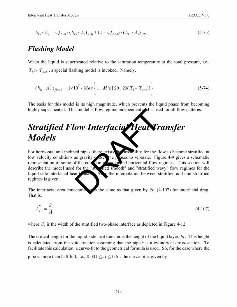
Interfacial Heat Transfer Models TRACE V5.0
. (5-73)
Flashing Model
When the liquid is superheated relative to the saturation temperature at the total pressure, i.e.,
, a special flashing model is invoked. Namely,
(5-74)
The basis for this model is its high magnitude, which prevents the liquid phase from becominghighly super-heated. This model is flow regime independent and is used for all flow patterns.
Stratified Flow Interfacial Heat Transfer ModelsFor horizontal and inclined pipes, there exists the possibility for the flow to become stratified atlow velocity conditions as gravity causes the phases to separate. Figure 4-9 gives a schematicrepresentation of some of the commonly recognized horizontal flow regimes. This section willdescribe the model used for the "stratified smooth" and "stratified wavy" flow regimes for theliquid-side interfacial heat transfer. Also, the interpolation between stratified and non-stratifiedregimes is given.
The interfacial area concentration is the same as that given by Eq. (4-107) for interfacial drag.That is,
(4-107)
where is the width of the stratified two-phase interface as depicted in Figure 4-12.
The critical length for the liquid-side heat transfer is the height of the liquid layer, hl . This heightis calculated from the void fraction assuming that the pipe has a cylindrical cross-section. Tofacilitate this calculation, a curve-fit to the geometrical formula is used. So, for the case where the
pipe is more than half full, i.e., , the curve-fit is given by
hki Ai· wfAM hki Ai·( )AM 1 wfAM–( ) hki Ai·( )BS·+·=
Tl Tsat>
hli Ai′′′·( )flash 1 7×10 Max 1 Min 20 20 Tl Tsat–( ),[ ],
⎩ ⎭⎨ ⎬⎧ ⎫
·=
Ai″′ Si
A----=
Si
0.001 α 0.5≤ ≤
DRAFT
216

TRACE V5.0 Interfacial Heat Transfer Models FOOBAR1234FOOBAR1234FOOBAR1234FOOBAR1234
Interfacial H
eat Transfer
Models
(5-75)
and if ,
(5-76)
Conversely, for the case where the pipe is more than half empty, i.e., , Eq. (5-75) andEq. (5-76) are rewritten as a function of the liquid volume fraction:
(5-77)
and if ,
(5-78)
For the liquid-side interfacial heat transfer coefficient, we have
, (5-79)
where the Nusselt no. is given by the same models as were used for the liquid film in annular flow[see Eqs. (5-49), (5-53), and (5-57)]. For stratified flow, however, the Reynolds no. is calculatedusing Eq. (4-197) which makes use of the "liquid-phase hydraulic diameter" defined byEq. (4-198).
For stratified flow, no data on interfacial condensation for the laminar flow regime was found.Though the K-S-P correlation was developed for condensation on slightly sheared falling films, ityields values only slightly greater than for steady conduction in laminar flow and thus shouldprovide a reasonable lower bound for the heat transfer.
For turbulent stratified flow, we have the data produced in the series of condensation experimentsconducted at Northwestern University. These experiments included test configurations for co-current horizontal flow (Ref. 5-10), counter-current horizontal flow (Ref. 5-16) with a pipeinclination angle of 4o, and counter-current vertical flow (Ref. 5-16) with a pipe inclination angleof 87o. Figure 5-4 compares all of the data from these three experiments to the models used inTRACE. For the co-current horizontal data, either the modified Bankoff or the adaptation of theGnielinski correlation used in TRACE, provides a reasonable lower bound to the data. As
hlD---- 1 0.70269591 α
2 3⁄0.34146667 α 0.161023911 α2·–·–·–=
α 0.001<
hlD---- 1 7.612668 α·–=
α 0.5>
hlD---- 0.70269591 αl
2 3⁄0.034146667 αl 0.161023911 αl
2·+·+·=
αl 0.001<
hlD---- 7.612668 αl·=
hliklhl---- Nuli·=
DRAFT
217

Interfacial Heat Transfer Models TRACE V5.0
explained above in Interfacial Heat Transfer Models for the Annular/Mist Flow Regime, asignificant entrance length effect was found in this data and the Bankoff correlation was reducedby 25% to better fit the data in the fully-developed region. Consequently, the data pointscorresponding to the inlet region are under-predicted.
The counter-current horizontal flow data are also reasonably well represented by the TRACEmodel as long as the film Reynolds no. has a value greater than about 104. However, for the
transition region, , the TRACE model consistently over-predicts theheat transfer for both the horizontal and vertical counter-current flow data.
Of more concern than the apparent over-prediction in the transition region is the capability of themodel to scale to larger Reynolds no. conditions. The maximum value in the NWU database is
only about , whereas in a PWR cold leg during ECC injection the Reynolds no. can range
from about during LPCI to about during accumulator injection for LBLOCAconditions. Consequently, due to the large amount of extrapolation that could be expected, theinterfacial heat transfer coefficient from Eq. (5-79) is limited to the maximum value present in theNWU database, namely
Figure. 5-4. Comparison of Bankoff and Gnielinski correlations with the Northwestern University condensation data.
! " #$
#%&' (
2 000 Ref 10 000,<<,
5 4×10
4 5×10 4 6×10
DRAFT
218

TRACE V5.0 Interfacial Heat Transfer Models FOOBAR1234FOOBAR1234FOOBAR1234FOOBAR1234
Interfacial H
eat Transfer
Models
(5-80)
Additionally, it should be noted that all of the NWU data was taken at atmospheric conditions andso pressure scaling could not be established.
Transition to Non-Stratified Flow
As was the case for the interfacial drag coefficients, there exists the potential for order-of-magnitude differences between the interfacial heat transfer for the stratified and non-stratifiedflow regimes. The section Stratified Flow Interfacial Drag Models in Chapter 4 detailed thecriteria used to determine whether or not the flow is stratified. The weighting factor for stratifiedflow, , determined in the calculation of the interfacial drag is also used for the interfacialheat transfer and is not repeated here [see Eq. (4-95) through Eq. (4-105)].
When the stratified flow weighting factor is greater than zero, the interfacial heat transfercoefficient is calculated from
(5-81)
where the exponent, n , is set equal to wfstrat .
Post-CHF Interfacial Heat Transfer ModelsThe post-CHF models are used to describe the interfacial heat transfer for the "inverted" flowregimes that occur when the surface temperature is too hot for the liquid phase to contact the wall.These regimes are shown schematically in Figure 4-13 and are the same as those described inChapter 4, Post-CHF Interfacial Drag Models.
The determination between the normal pre-CHF flow regimes and the inverted post-CHF flowregimes is made using the axial locations of the bottom and top quench fronts. For mass/energycomputational volumes that are completely quenched, the normal pre-CHF regimes are used.Whereas, for computational volumes whose heat transfer surface is in film boiling, (i.e., they arelocated entirely between the top and bottom quench fronts), the inverted post-CHF regimes areused. Finally, for computational volumes that are partially quenched, an interpolation betweenthe interfacial heat transfer for pre- and post-CHF values is performed as explained in Transitionto Pre-CHF Regimes.
Three principal inverted flow regimes are modeled in TRACE for post-CHF conditions: invertedannular, inverted slug, and dispersed flow. The region over which each of these post-CHFregimes is applied is shown in Figure 4-14. The models used for the evaluation of the interfacial
hli Min 2.5 4×10 hli, =
wfstrat
hli Ai· hli Ai·( )stratn
hli Ai·( )ns1 n–( )
·=
DRAFT
219

Interfacial Heat Transfer Models TRACE V5.0
heat transfer for each of these flow regimes are described in the following sections along with thetransition to pre-CHF regimes.
Inverted Annular
During film boiling, when the liquid phase is significantly subcooled, only a thin vapor filmseparates the hot surface from the subcooled liquid core. This regime is called inverted annularfilm boiling and the heat transfer paths are as depicted in Figure 5-5. Most of the heat transferfrom the wall is across the vapor film to the saturated liquid interface and thence into thesubcooled liquid core. Experimental data indicate that the inverted annular regime persists up tovoid fractions of 60-70% and that a smooth transition is made to the dispersed flow regime. InTRACE, the inverted annular regime is assumed to exist for void fractions up to 60%. Thissection describes the models used for the two interfacial heat transfer paths: vapor-interface andinterface-liquid.
Figure. 5-5. Schematic of heat transfer paths for inverted annular film boiling.
Vapor Liquid
Qwv Qvi Qli
TsatTv
Tw
Qrad
TliqDRAFT
220
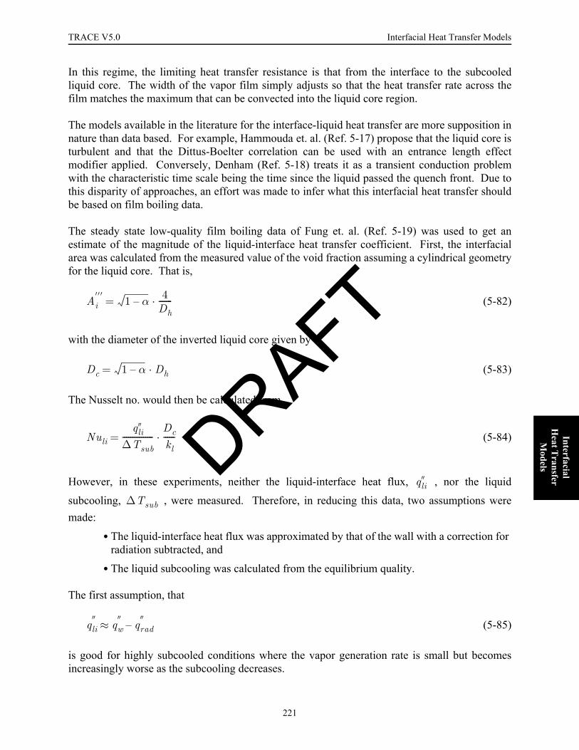
TRACE V5.0 Interfacial Heat Transfer Models FOOBAR1234FOOBAR1234FOOBAR1234FOOBAR1234
Interfacial H
eat Transfer
Models
In this regime, the limiting heat transfer resistance is that from the interface to the subcooledliquid core. The width of the vapor film simply adjusts so that the heat transfer rate across thefilm matches the maximum that can be convected into the liquid core region.
The models available in the literature for the interface-liquid heat transfer are more supposition innature than data based. For example, Hammouda et. al. (Ref. 5-17) propose that the liquid core isturbulent and that the Dittus-Boelter correlation can be used with an entrance length effectmodifier applied. Conversely, Denham (Ref. 5-18) treats it as a transient conduction problemwith the characteristic time scale being the time since the liquid passed the quench front. Due tothis disparity of approaches, an effort was made to infer what this interfacial heat transfer shouldbe based on film boiling data.
The steady state low-quality film boiling data of Fung et. al. (Ref. 5-19) was used to get anestimate of the magnitude of the liquid-interface heat transfer coefficient. First, the interfacialarea was calculated from the measured value of the void fraction assuming a cylindrical geometryfor the liquid core. That is,
(5-82)
with the diameter of the inverted liquid core given by
(5-83)
The Nusselt no. would then be calculated from
(5-84)
However, in these experiments, neither the liquid-interface heat flux, , nor the liquid
subcooling, , were measured. Therefore, in reducing this data, two assumptions weremade:
•The liquid-interface heat flux was approximated by that of the wall with a correction for radiation subtracted, and
•The liquid subcooling was calculated from the equilibrium quality.
The first assumption, that
(5-85)
is good for highly subcooled conditions where the vapor generation rate is small but becomesincreasingly worse as the subcooling decreases.
Ai′′′ 1 α– 4
Dh-------·=
Dc 1 α– Dh·=
Nuliqli″
∆Tsub----------------
Dckl------·=
qli″
∆Tsub
qli″ qw
″ qrad″–≈
DRAFT
221
Interfacial Heat Transfer Models TRACE V5.0
Figure 5-6 shows the results of this data analysis for the experiments of Fung (Ref. 5-19) using theabove two assumptions. The first thing to note is that there is little if any dependence upon themass flux, so using a model for turbulent forced convection, such as Dittus-Boelter, is probablynot correct. Second, at high values of the liquid subcooling, where the assumption given byEq. (5-85) is considered valid, it appears that the inferred Nusselt no. approaches an asymptoticvalue. This leads then to the proposed model,
(5-86)
that is similar to that of Saha and Zuber (Ref. 5-20) for subcooled boiling at low Peclet nos.,namely
(5-87)
This simple constant value for the liquid-interface Nusselt no. was chosen as the model forTRACE. However, in simulations of FLECHT-SEASET high flooding rate tests, this valueappeared to be too large and thus was reduced to
. (5-88)
Also, in Figure 5-6, a large increase in the liquid-interface Nusselt no. is indicated as thesubcooling decreases to zero. At least part of this large increase results from the assumptiongiven by Eq. (5-85) becoming invalid. However, as the liquid core approaches saturation andvapor generation increases dramatically, the surface of the core becomes rough and the entire corecan oscillate. So, it is possible that some of this apparent enhancement is real though no attemptto model it is made in TRACE.
For the vapor-interface heat transfer, the model chosen was laminar convection in a thin film.That is,
(5-89)
The characteristic length, , is the vapor film thickness, which is computed from the void fractionusing geometric formula either for a tube or a rod bundle. For the rod bundle case, the filmthickness is then
(5-90)
where (P/Dr) is the pitch-to-diameter ratio, and for a tube geometry
Nuli 200≈
Nuli 455≈
Nuli 100≈
hvi 2kgδ-----·=
δ
δDh2
------- 1 α 4π--- P
Dr------
⎝ ⎠⎜ ⎟⎛ ⎞
2
1–·+ 1–
⎩ ⎭⎪ ⎪⎨ ⎬⎪ ⎪⎧ ⎫
·=
DRAFT
222

TRACE V5.0 Interfacial Heat Transfer Models FOOBAR1234FOOBAR1234FOOBAR1234FOOBAR1234
Interfacial H
eat Transfer
Models
(5-91)
In both Eq. (5-90) and Eq. (5-91), the void fraction is limited to be greater than 0.01 to keep themagnitude of the resulting heat transfer coefficient from getting unreasonably large.
Two heat transfer coefficients remain to be specified: that for gas-liquid sensible heat transfer andthat for flashing. Neither of these is considered to be important for inverted annular film boiling,but both must be specified to complete the mathematical model. First, for the case of sensibleheat transfer, the gas-liquid heat transfer coefficient is taken to be the same as that for the vapor-interface,
(5-92)
which assumes that the liquid-side heat transfer resistance is negligible.
Flashing occurs when the liquid temperature exceeds saturation. This is not expected to occur ininverted annular film boiling as the associated large vapor generation rate would rapidly lead tobreakup and entrainment of the liquid core. However, to ensure that unreasonably large values ofliquid superheat do not occur, the interfacial heat transfer coefficient given by Eq. (5-88) is
Figure. 5-6. Inferred values of the Nusselt no. for liquid-interface heat transfer for the low-quality film boiling data of Fung.
! " #$%
! " #$%
! " #$%
! " #$%
! " #$%
! " #$%
δDh2
------- 1 1 α––( )·=
hgl hvi=
DRAFT
223

Interfacial Heat Transfer Models TRACE V5.0
ramped to a large value as a function of liquid superheat. The so-called "F12" multiplier of theRELAP5 code (Ref. 5-21) is used to accomplish this ramping. Thus,
(5-93)
where is the liquid superheat.
This completes the description for the models used in the inverted annular film boiling regime.Film boiling data indicates that there is a smooth transition from inverted annular film boiling todispersed flow. As no models were available for this "transition region", a simple interpolationprocedure is used as discussed below in Interpolation Region. First, the models for invertedslugs and dispersed droplets that provide the other point for the interpolation scheme aredescribed.
Inverted Slug
As the liquid core approaches saturation and the vapor generation rate increases, the liquid coredisintegrates into a mixture of ligaments and droplets. In TRACE, breakup of the invertedannular liquid core is assumed to begin at a void fraction of 60% and to be complete at a voidfraction of 90%. Between these two values, an "interpolation region" is used to provide a smoothtransition as described below. For void fractions above 90%, the liquid phase is assumed to becomposed entirely of a mixture of small, dispersed droplets and large liquid fragments, or"inverted slugs" with the determination between these two forms being given by the entrainmentfraction. This section describes the interfacial heat transfer models for the liquid considered to bein the form of inverted slugs.
The fraction of the liquid considered to be in the form of dispersed droplets is given by theentrained fraction and is computed using Eqs. (4-159) and (4-160), while the remainder of theliquid is treated as inverted slugs. The interfacial heat transfer is then calculated using a simplelinear weighting scheme, for example,
(5-94)
where E is the entrainment fraction.
As discussed for interfacial drag in Chapter 4, Inverted Slug Regime, the inverted slugs areidealized as prolate ellipsoids with an aspect ratio of 4.5. The surface area of a prolate ellipsoid isgiven by
(5-95)
hli( )flash hli 1 ∆Tsup 250 50 ∆Tsup·+( )·+·=
Tsup∆
hli Ai· 1 E–( ) hli Ai·( )IS E hli Ai·( )DF·+·=
S 2π a2 2πa b·e
---------- e( )asin· ·+·=
DRAFT
224
TRACE V5.0 Interfacial Heat Transfer Models FOOBAR1234FOOBAR1234FOOBAR1234FOOBAR1234
Interfacial H
eat Transfer
Models
where and are respectively the minor and major radii and is the ellipticity defined by
(5-96)
For a ligament with an aspect ratio of 4.5, the ellipticity is then equal to 0.975 and the surface areareduces to
(5-97)
Then, using Eq. (4-123) for the ligament volume, the surface area per unit volume is
(5-98)
where is the diameter of the ligament, that is, twice the minor radius.
To evaluate the interfacial area, it remains to specify the ligament diameter. As a firstapproximation, the diameter of the inverted annular core at breakup is used. Then, using a voidfraction of 60% as the upper limit for the inverted annular regime, we have
(5-99)
To compute the interfacial heat transfer coefficients, the models described below for dispersedflow are used. For large droplets, such as an inverted slug, one modification to the disperseddroplet models is made. Specifically, the liquid-side heat transfer coefficient is increased by up toa factor of 4 for large drops in order to account for the effects of shape oscillation as noted byHijikata et. al. (Ref. 5-22). In practice, this enhancement helps to eliminate any residualsubcooling that might exist from the inverted slugs in a region close to where they are formed.This enhancement factor is an engineering approximation and is given by
(5-100)
where dRT is the Sauter mean diameter for a distribution having a maximum diameter that isstable against the Rayleigh-Taylor instability. Using the formula of Kitsch andKocamustafaogullari (Ref. 4-44), then gives
(5-101)
a b e
e 1 ab---
⎝ ⎠⎛ ⎞
2–=
S 7.2156 2π a2··=
Ai′′′( )IS
4.8104 1 α–( )·dIS
---------------------------------------=
dIS
dIS 0.6325 Dh·≈
hli′ hli 4 Min 1dISdRT----------⎝ ⎠
⎛ ⎞2
,· ·=
dRT3.524
---------- σg ∆ρ·---------------·=
DRAFT
225

Interfacial Heat Transfer Models TRACE V5.0
The following section details all of the droplet heat transfer models used in TRACE for post-CHFconditions.
Dispersed Flow
The fraction of the liquid that is entrained is treated as dispersed droplets that are relatively smalland nearly spherical. The droplet diameter for interfacial heat transfer is calculated from the samemodels as previously described for post-CHF interfacial drag in Chapter 4, Post-CHF FlowRegimes (see Eqs. (4-134) through (4-145)). The interfacial area concentration is then
(5-102)
in terms of the droplet Sauter mean diameter.
For post-CHF conditions, the most important interfacial heat transfer process is that for the gas-side as it limits the steam superheat and thereby directly affects the peak clad temperature. Thegas-side heat transfer coefficient is given by
(5-103)
For the gas-side drop Nusselt no., the model of Renksizbulut & Yuen (Ref. 5-23) was chosengiving
(5-104)
as a function of the droplet Reynolds no. This correlation is stated to be valid for the range
The major difference between Eq. (5-104) and the model of Ranz-Marshall is the inclusion of a"blowing factor", , to account for the effects of mass transfer upon heat transfer. In addition,the vapor transport properties used in Eq. (5-104) are evaluated at a reference film temperature asindicated by the second " " subscript. However, in TRACE, we have elected to simply use the
Ai′′′ 6 1 α–( )·
dSM-------------------------=
hvikg
dSM---------- Nud·=
Nud f,
1 Bf+[ ]0.7· 2 0.57 Red f,
1 2⁄Pr
g f,
1 2⁄··+=
25 Red f,
2000≤≤
0.07 Bf 2.79≤ ≤
150 Tg Tsat–( ) 700°C≤ ≤
Bf
f
DRAFT
226
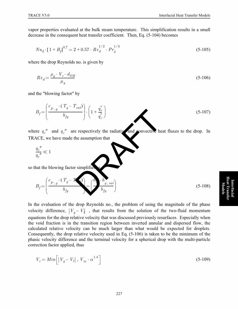
TRACE V5.0 Interfacial Heat Transfer Models FOOBAR1234FOOBAR1234FOOBAR1234FOOBAR1234
Interfacial H
eat Transfer
Models
vapor properties evaluated at the bulk steam temperature. This simplification results in a smalldecrease in the consequent heat transfer coefficient. Then, Eq. (5-104) becomes
(5-105)
where the drop Reynolds no. is given by
(5-106)
and the "blowing factor" by
(5-107)
where and are respectively the radiative and convective heat fluxes to the drop. InTRACE, we have made the assumption that
so that the blowing factor simplifies to
(5-108)
In the evaluation of the drop Reynolds no., the problem of using the magnitude of the phasevelocity difference, , that results from the solution of the two-fluid momentumequations for the drop relative velocity that was discussed previously resurfaces. Especially whenthe void fraction is in the transition region between inverted annular and dispersed flow, thecalculated relative velocity can be much larger than what would be expected for droplets.Consequently, the drop relative velocity used in Eq. (5-106) is taken to be the minimum of thephasic velocity difference and the terminal velocity for a spherical drop with the multi-particlecorrection factor applied, thus
(5-109)
Nud 1 Bf+[ ]0.7· 2 0.57 Red1 2⁄
Prg1 3⁄
··+=
Redρg Vr dSM· ·
µg-------------------------------=
Bf
cP g,
Tg Tsat–( )·
hfg--------------------------------------------
⎝ ⎠⎜ ⎟⎜ ⎟⎛ ⎞
1qr″
qc″
-----+⎝ ⎠⎜ ⎟⎛ ⎞
·=
qr″ qc″
qr″qr″------- 1
Bf
cP g,
Tg Tsat–( )·
hfg--------------------------------------------
⎝ ⎠⎜ ⎟⎜ ⎟⎛ ⎞ hg h
g sat,–
hfg--------------------------
⎝ ⎠⎜ ⎟⎛ ⎞
= =
Vg Vl–
Vr Min Vg Vl– V∞ α1.4·,=
DRAFT
227

Interfacial Heat Transfer Models TRACE V5.0
For the single-particle terminal velocity, , the formula of Wallis given in Eq. (4-135) is usedagain. Also, the reflood Sauter mean drop diameter from Eq. (4-138) and Eq. (4-145) wassubstituted into Eq. (4-135) to yield
(5-110)
For the liquid-side heat transfer, hli , the asymptotic value of Kronig & Brink (Ref. 5-14) given byEq. (5-63) is used. For the gas-liquid sensible heat transfer, we assume that the liquid-side heattransfer resistance is much smaller than the gas-side, and so the gas-side interfacial heat transfercoefficient from Eq. (5-105) is used. That is,
(5-111)
Finally, as was done for the inverted annular regime, see Eq. (5-93), the flashing interfacial heattransfer is computed by applying the "F12" multiplier from RELAP5 to the liquid-side heattransfer coefficient.
Interpolation Region
Experimental data indicate that the inverted annular regime persists up to void fractions of 60-70% and that a smooth transition is made to the dispersed flow regime. The role of theinterpolation region is to provide this smooth transition. As shown in Figure 4-14, the invertedannular regime is assumed for void fractions less than 60%, while for void fractions greater than90%, the flow consists of a mixture of inverted slugs and droplets. Between these two limits, thefollowing interpolation scheme is used.
First, the interfacial heat transfer for the inverted annular regime is calculated, as denoted by thesubscript "IA". Next, the interfacial heat transfer is re-calculated treating the liquid phase as amixture of dispersed droplets and inverted slugs with the subscripts "DF" and "IS" denoting thevalues for dispersed flow and inverted slugs respectively. Then, the weighting factor for invertedannular flow is calculated from
(5-112)
where
(5-113)
Finally, the contributions from the inverted annular and the dispersed flow or inverted slugregimes are combined as illustrated for the case of the liquid-side heat transfer by
V∞
V∞ 0.6σ0.316 g ∆ρ·( )
0.228
ρg0.456µg
0.0879---------------------------------------------·=
hgl hvi=
wfIA 2 xIA xIA2–·=
xIA0.9 α–0.9 0.6–---------------------⎝ ⎠
⎛ ⎞=
DRAFT
228
TRACE V5.0 Interfacial Heat Transfer Models FOOBAR1234FOOBAR1234FOOBAR1234FOOBAR1234
Interfacial H
eat Transfer
Models
(5-114)
This same interpolation formula is used for the other interfacial heat transfer coefficients and forthe wall heat transfer coefficient (see Chapter 6, Inverted Slug Film Boiling).
Transition to Pre-CHF Regimes
The determination between the normal pre-CHF flow regimes and the inverted post-CHF flowregimes is made using the axial locations of the bottom and top quench fronts. For mass/energycomputational volumes that are completely quenched, the normal pre-CHF regimes are used.Whereas, for computational volumes whose heat transfer surface is in film boiling, (i.e., they arelocated entirely between the top and bottom quench fronts), the inverted post-CHF regimes areused. Finally, for computational volumes that are partially quenched, an interpolation betweenthe interfacial heat transfer for pre- and post-CHF values is performed.
Let represent the fraction of the mass/energy computational volume that is quenched. Theinterfacial heat transfer coefficients are then computed using a simple linear interpolation scheme.For example, for the liquid-side heat transfer,
(5-115)
This same linear interpolation is used for all of interfacial heat transfer coefficients.
However, before Eq. (5-115) is applied to the liquid-side heat transfer, one modification is made.Specifically, the liquid-side heat transfer coefficient for the pre-CHF regime is constrained to begreater than that for the post-CHF regime as would be expected.
Non-Condensable Gas EffectsWhen non-condensable gases are present, the mass transfer processes of condensation andevaporation are both affected in two ways. First, the driving temperature difference is reduced inthe case of condensation, as
or, increased in the case of evaporation, as
hli Ai· wfIA hli Ai·( )IA 1 wfIA–( ) E hli Ai·( )DF 1 E–( ) hli Ai·( )IS·+·[ ]+·=
fQ
hli Ai· fQ hli Ai·( )pre CHF– 1 fQ–( ) hli Ai·( )post CHF–·+·=
Tsv Tl Tsat Tl–≤–
Tl Tsv Tl Tsat–≥–
DRAFT
229

Interfacial Heat Transfer Models TRACE V5.0
where is the saturation temperature at the vapor bulk partial pressure for the mass/energycomputational cell. Secondly, the mass transfer rate can become limited by the rate at which thenon-condensable gas can diffuse either away from (condensation) or towards the interface(evaporation).
The models used by TRACE to modify the liquid-side interfacial heat transfer when non-condensable gases are present are described below. Both the default model for condensation andthe model for evaporation were retained from the TRAC-PF1/MOD2 code. However, to improveTRACE's predictive capability for both in-tube condensation for the PCCS component and forwall condensation in the drywell of the proposed ESBWR design, a new model for the effects ofnon-condensable gases upon film condensation was added to the TRACE code. This new modelis described in Special Model for Film Condensation below and is expected to replace the defaultmodel in a future code release after more testing has been completed.
For the effect of non-condensable gases upon the gas-side heat transfer, the interfacial heattransfer coefficient determined using the models described above is multiplied by the relativepartial pressure in the energy equation. Thus,
(5-116)
which forces the vapor-interface heat transfer to zero as the vapor is depleted.
Also, when non-condensable gases are present, allowance is made for the sensible heat transferbetween the gas mixture and the liquid phase. The gas-liquid heat transfer coefficients describedabove are similarly multiplied by the relative partial pressure of the non-condensable gas, so that
(5-117)
and the sensible heat transfer goes to zero as pure-steam conditions are approached.
Default Model for Condensation
During condensation driven by interfacial heat transfer for pure-steam conditions, the limitingheat transfer resistance is usually that between the interface and the subcooled liquid. When non-condensable gases are present, the concentration of the non-condensable gas builds up at theinterface, thereby lowering the local vapor partial pressure and hence the temperature of theinterface below that for saturation of the bulk gas mixture. That is,
Tsv
qvi″PvP------ hvi Tg Tsv–( )· ·=
qgl″ PNC
P----------- hgl Tg Tl–( )· ·=
Ti Tsv≤
DRAFT
230

TRACE V5.0 Interfacial Heat Transfer Models FOOBAR1234FOOBAR1234FOOBAR1234FOOBAR1234
Interfacial H
eat Transfer
Models
and so the driving potential for condensation is reduced even further and the condensation ratecan become limited by the rate at which the non-condensable gas can diffuse away from theinterface.
The two-fluid numerical scheme of TRACE includes a non-condensable gas field and so the bulkvapor partial pressure is calculated for every mass/energy computational volume. The interfacialheat transfer rates that drive mass transfer, are then defined in terms of the cell's bulk conditions,for example
(5-118)
rather than in terms of the local interface temperature. The non-condensable gas effect describedabove then must be added as an effective heat transfer resistance on the liquid-side heat transfer,so that
(5-119)
where the second subscript "NC" indicates that the additional resistance due to diffusion of thenon-condensable gas away from the interface has been added to that of the liquid-side heattransfer.
The TRACE default model is the empirical correlation of Sklover and Rodivilin (Ref. 5-24) and it
is invoked whenever and the special film condensation model is not selected (seebelow). The original form of this correlation was developed for subcooled water jets with an air-steam crossflow and was given by
(5-120)
where is the liquid-side heat transfer coefficient in the presence of non-condensables, and
Ga, Gl , and Gs are the air, water, and steam mass fluxes, respectively. The experimental basisfor the Sklover and Rodivilin correlation covered the following liquid and steam mass fluxranges,
but the range for the air mass flux was not specified.
qli″ hli Tl Tsv–( )·=
qli″ h
li NC,Tl Tsv–( )· hli Tl Ti–( )·= =
Tl Tsv≤
hli NC,
hli---------------- 0.366
GaGl
Gs2
-------------⎝ ⎠⎜ ⎟⎛ ⎞
0.2–·=
hli NC,
3000 Gl 18000 kg m2s⁄( )≤ ≤
100 Gs 710 kg m2s⁄( )≤ ≤
DRAFT
231

Interfacial Heat Transfer Models TRACE V5.0
In TRACE, the mixture of condensable and non-condensable gases flows with the same velocity.Thus, Eq. (5-120) reduces to
(5-121)
which is finally rewritten in terms of the gas mixture density and non-condensable gas density as
(5-122)
In the evaluation of Eq. (5-122), the mass fluxes are limited to be in the ranges,
(5-123)
and the reduction factor is limited to the range
(5-124)
The above model is strictly applicable only to the specific configuration for which it wasdeveloped, that is, a subcooled liquid jet in an air-steam crossflow. It is not applicable to otherconfigurations and being highly empirical, extrapolation beyond its database will lead toquestionable results. This model will be replaced in a future TRACE update by he mass transferbased model described below in Special Model for Film Condensation as soon as sufficienttesting has been conducted to assure the accuracy and robustness of the new model.
Special Model for Film Condensation
For the proposed ESBWR design, a critical component is the Passive Containment CoolingSystem (PCCS) that removes decay heat from the drywell via in-tube condensation of a steam-gasmixture. To improve the predictive capability of the TRACE code for the PCCS component, anew model for condensation in the presence of non-condensable gases was developed asdescribed below. Later, this model was extended to also be applicable to condensation on thewalls of the drywell itself. It is intended that this new model will become the default in TRACEreplacing the Sklover-Rodivilin correlation in a future update once it has been extended to theother flow regimes and sufficient testing has been completed. For this code release though, the"special film condensation model" has to be invoked for each component using the "PipeType" or"VessType" input parameters as described in the user's guide.
hli NC,
hli---------------- 0.366
ρsρNC----------
⎝ ⎠⎜ ⎟⎛ ⎞
0.2 GsGl------
⎝ ⎠⎜ ⎟⎛ ⎞0.2
· ·=
hli NC,
hli---------------- 0.366
ρg ρNC–ρNC
---------------------⎝ ⎠⎜ ⎟⎛ ⎞
0.2GsGl------
⎝ ⎠⎜ ⎟⎛ ⎞
0.2
· ·=
3000 Gl 18000 kg m2s⁄( )≤ ≤
0 Gs 640 kg m2s⁄( )≤ ≤
0.1h
li NC,
hli---------------- 1.0≤ ≤
DRAFT
232
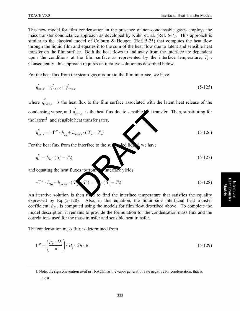
TRACE V5.0 Interfacial Heat Transfer Models FOOBAR1234FOOBAR1234FOOBAR1234FOOBAR1234
Interfacial H
eat Transfer
Models
This new model for film condensation in the presence of non-condensable gases employs themass transfer conductance approach as developed by Kuhn et. al. (Ref. 5-7). This approach issimilar to the classical model of Colburn & Hougen (Ref. 5-25) that computes the heat flowthrough the liquid film and equates it to the sum of the heat flow due to latent and sensible heattransfer on the film surface. Both the heat flows to and away from the interface are dependentupon the conditions at the film surface as represented by the interface temperature, Ti .Consequently, this approach requires an iterative solution as described below.
For the heat flux from the steam-gas mixture to the film interface, we have
(5-125)
where is the heat flux to the film surface associated with the latent heat release of the
condensing vapor, and is the heat flux due to sensible heat transfer. Then, substituting for
the latent1 and sensible heat transfer rates,
(5-126)
For the heat flux from the interface to the subcooled liquid, we have
(5-127)
and equating the heat fluxes to/from the interface yields,
(5-128)
An iterative solution is then used to find the interface temperature that satisfies the equalityexpressed by Eq. (5-128). Also, in this equation, the liquid-side interfacial heat transfercoefficient, hli , is computed using the models for film flow described above. To complete themodel description, it remains to provide the formulation for the condensation mass flux and thecorrelations used for the mass transfer and sensible heat transfer.
The condensation mass flux is determined from
(5-129)
1. Note, the sign convention used in TRACE has the vapor generation rate negative for condensation, that is,
.
qmix″ qcond
″ qsens″+=
qcond″
qsens″
Γ 0<
qmix″ Γ″ hfg hsens Tg Ti–( )·+·–=
qli″ hli Ti Tl–( )·=
Γ″ hfg hsens Tg Ti–( )·+·– hli Ti Tl–( )·=
Γ″ρg D0·
d-----------------
⎝ ⎠⎜ ⎟⎛ ⎞
Bf Sh b·· ·=
DRAFT
233

Interfacial Heat Transfer Models TRACE V5.0
where is the density of the gas-steam mixture at free-stream conditions, D0 is the diffusioncoefficient, and d is the characteristic length. The mass transfer driving potential, b , is given by
(5-130)
in terms of the vapor mass fraction for the interface, , and for the free-stream, . The
vapor mass fraction at the interface is
(5-131)
where the vapor density is computed for saturation conditions at a partial pressure correspondingto the interface temperature. That is,
(5-132)
and
(5-133)
The density of the non-condensable gas is similarly evaluated as a function of its partial pressureand the interface temperature.
The Sherwood no., , will be evaluated from standard heat transfer correlations using the heat-mass transfer analogy as discussed below. Finally, , is the "blowing factor" that accounts forthe effects of mass transfer upon the diffusion of steam towards the interface and is given by
(5-134)
according to Eq. (18-9) of Reference 5-26.
The sensible heat flux is given by
ρg
bx
v ∞,x
v i,–
⎝ ⎠⎛ ⎞
xv i,
1–⎝ ⎠⎛ ⎞
----------------------------------=
xv i,
xv ∞,
xv i,
ρv i,
ρv ρNC+( )i
----------------------------=
Pv i,
Pv sat,
Ti( )=
ρv i,
ρv sat,
Pv i,⎝ ⎠
⎛ ⎞=
ShBf
Bf1 b+( )lnb
-----------------------=
DRAFT
234
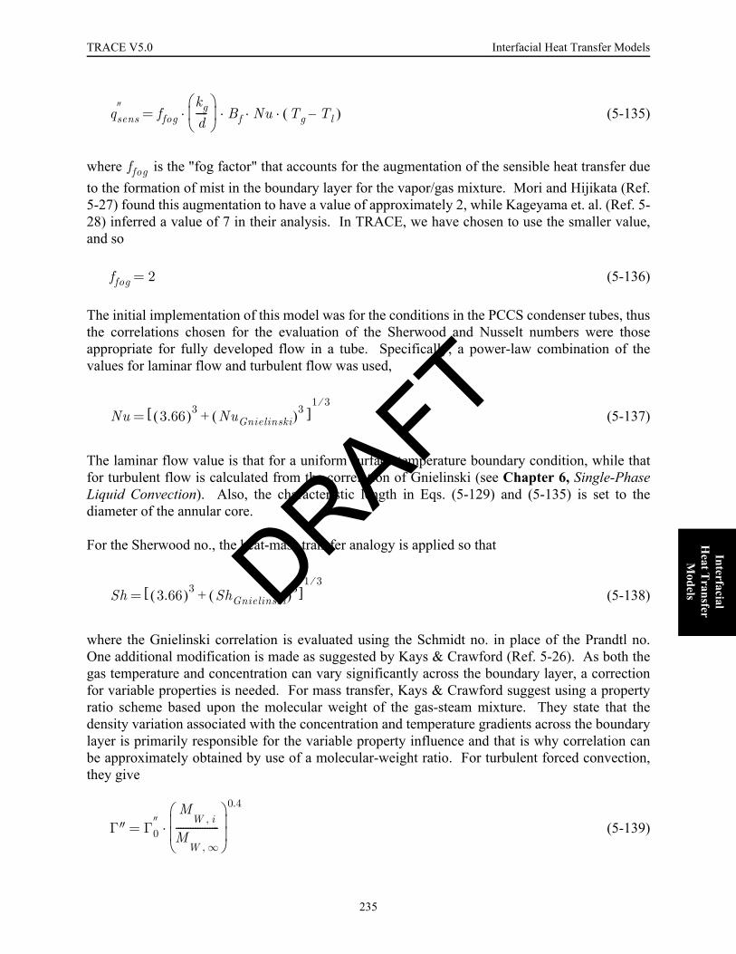
TRACE V5.0 Interfacial Heat Transfer Models FOOBAR1234FOOBAR1234FOOBAR1234FOOBAR1234
Interfacial H
eat Transfer
Models
(5-135)
where is the "fog factor" that accounts for the augmentation of the sensible heat transfer dueto the formation of mist in the boundary layer for the vapor/gas mixture. Mori and Hijikata (Ref.5-27) found this augmentation to have a value of approximately 2, while Kageyama et. al. (Ref. 5-28) inferred a value of 7 in their analysis. In TRACE, we have chosen to use the smaller value,and so
(5-136)
The initial implementation of this model was for the conditions in the PCCS condenser tubes, thusthe correlations chosen for the evaluation of the Sherwood and Nusselt numbers were thoseappropriate for fully developed flow in a tube. Specifically, a power-law combination of thevalues for laminar flow and turbulent flow was used,
(5-137)
The laminar flow value is that for a uniform surface temperature boundary condition, while thatfor turbulent flow is calculated from the correlation of Gnielinski (see Chapter 6, Single-PhaseLiquid Convection). Also, the characteristic length in Eqs. (5-129) and (5-135) is set to thediameter of the annular core.
For the Sherwood no., the heat-mass transfer analogy is applied so that
(5-138)
where the Gnielinski correlation is evaluated using the Schmidt no. in place of the Prandtl no.One additional modification is made as suggested by Kays & Crawford (Ref. 5-26). As both thegas temperature and concentration can vary significantly across the boundary layer, a correctionfor variable properties is needed. For mass transfer, Kays & Crawford suggest using a propertyratio scheme based upon the molecular weight of the gas-steam mixture. They state that thedensity variation associated with the concentration and temperature gradients across the boundarylayer is primarily responsible for the variable property influence and that is why correlation canbe approximately obtained by use of a molecular-weight ratio. For turbulent forced convection,they give
(5-139)
qsens″ ffog
kgd-----
⎝ ⎠⎜ ⎟⎛ ⎞
Bf Nu Tg Tl–( )·· · ·=
ffog
ffog 2=
Nu 3.66( )3 NuGnielinski( )3+[ ]1 3⁄
=
Sh 3.66( )3 ShGnielinski( )3+[ ]1 3⁄
=
Γ″ Γ0″
MW i,
MW ∞,
------------------⎝ ⎠⎜ ⎟⎜ ⎟⎛ ⎞ 0.4
·=
DRAFT
235

Interfacial Heat Transfer Models TRACE V5.0
where is the condensation mass flux for constant properties evaluated at free-streamconditions.
Once the iterative solution for the interface temperature has converged, the condensation rate isknown and the resulting interfacial heat transfer coefficients can be determined. In terms of theinterface temperature, the condensation rate is then
(5-140)
and so the liquid-side interfacial heat transfer coefficient in the presence of non-condensablegases becomes
(5-141)
Similarly, the heat flux associated with the sensible heat transfer from the gas mixture to theinterface is translated into a heat transfer coefficient using the gas-liquid temperature differenceas the driving potential. Namely,
(5-142)
The choice was made to use a more mechanistic approach, i.e., a mass transfer conductancemodel, for the effect of non-condensable gases upon condensation not only because it is morephilosophically appealing but because it also has the potential to be more accurate. For example,Kuhn et. al. (Ref. 5-7) noted that for their database, the mass transfer conductance model wasmore accurate than a purely empirical model developed from that same data. We compared theabove TRACE model to all of the air-steam and helium-steam data in the experiments of Kuhn.There were 72 air-steam tests giving a total of 571 data points, the TRACE model calculated theheat transfer coefficient for these with an average error of 12.5% and an RMS error of 20.5%.Similarly, there were 25 helium-steam tests giving a total of 192 data points, the TRACE modelcalculated the heat transfer coefficient for these with an average error of 0.9% and an RMS errorof 16.3%. These values are considered to be within the error bands associated with this data.
Later, it was decided to extend this film condensation model to also be applicable for theconditions of the drywell walls in the ESBWR design. For large containment volumes, thecorrelations used for turbulent forced convection to evaluate the Nusselt and Sherwood numbersneeded to be replaced by something more appropriate. For this purpose, the correlation forturbulent free convection on a vertical plate given by McAdams (Ref. 5-29) was chosen. That is,
Γ0″
Γ″ hfg· hli Tl Ti–( )·=
hli NC,
Γ″ hfg·Tl Tsv–( )
------------------------- hliTl Ti–( )Tl Tsv–( )
-------------------------·= =
hgl hsensTg Ti–( )Tg Tl–( )
-----------------------·=
NuL 0.13 GrL Prg·( )1 3⁄
·=
DRAFT
236
TRACE V5.0 Interfacial Heat Transfer Models FOOBAR1234FOOBAR1234FOOBAR1234FOOBAR1234
Interfacial H
eat Transfer
Models
(5-143)
where the subscript L indicates that it is the average over a plate of that length. The Grashof no. iscalculated from the density difference between the interface and the free-stream. Thus,
(5-144)
Note that because the characteristic length scale, , in Eq. (5-144) is cubed, and the Grashof no.is taken to the one-third power, the dependence upon the length scale is absent from the resultingheat and mass transfer coefficients. Consequently, in TRACE, the hydraulic diameter is used forthis length scale but has no effect upon the results.
Similar to the situation for turbulent forced convection, a correction for variable properties is alsoneeded for the free convection case. Failing to find a suitable correction factor in the literature, amodel was derived along the lines of that proposed by Kays and Crawford (Ref. 5-26) for theforced convection case. The resulting correction yields
(5-145)
for the case of turbulent free convection.
A comparison of this model was made to both the Uchida correlation (Ref. 5-30) and the Dehbidata (Ref. 5-31) with excellent results. Figure 5-7 presents this comparison to the Uchidacorrelation over a wide range of non-condensable gas mass fraction for atmospheric pressureconditions.
Finally, to eliminate the need for the user to select either "tube" or "wall" condensation, thecorrelations used to evaluate the Sherwood and Nusselt numbers for free and forced convectionwere combined. Simply stated, the maximum value for either free or forced convection is used.For example,
(5-146)
As stated above, this model is invoked by the user through the specification of the PIPETYPE orVESSTYPE input variables for 1-D and 3-D components, respectively. When this model hasbeen extended to the remaining flow regimes and sufficiently tested, it will become the defaultmodel for the effects of non-condensable gases upon condensation. At present, its application islimited to the annular flow regime.
ShL 0.13 GrL Scg·( )1 3⁄
·=
GrL
L3 g ρg ρg i,
–· ·
ρg νg2·
--------------------------------------------=
L
Γ″ Γ0″
MW i,
MW ∞,
------------------⎝ ⎠⎜ ⎟⎜ ⎟⎛ ⎞ 0.57
·=
Nu Max NuNC NuFC,=
DRAFT
237

Interfacial Heat Transfer Models TRACE V5.0
Model for Evaporation
When non-condensable gases are present, , and evaporation due to interfacial heat
transfer can occur whenever . For this case, the vapor generation increases theconcentration of steam at the interface, thereby increasing the local interface temperature anddecreasing the evaporation rate. When a significant fraction of non-condensable gases arepresent, evaporation can then be governed by the rate at which the non-condensable gas candiffuse towards the interface. In TRACE, this is modeled by adding the resistance to heat transferassociated with this diffusion to that of the heat transfer within the liquid phase. That is,
(5-147)
where denotes the effective interfacial heat transfer resistance associated with thediffusion process.
Figure. 5-7. Comparison of the TRACE model for wall condensation in the presence of non-condensable gases with the Uchida correlation at atmospheric pressure.
! "
#$
%&' !
Tsv Tsat<
Tl Tsv≥
hli NC,
1hli------ 1
hevap------------+
1–
=
1 hevap⁄
DRAFT
238

TRACE V5.0 Interfacial Heat Transfer Models FOOBAR1234FOOBAR1234FOOBAR1234FOOBAR1234
Interfacial H
eat Transfer
Models
To provide a reasonable estimate for , a simple diffusion model is used. The mass transfercoefficient is obtained from
(5-148)
where the Sherwood, Schmidt, and Reynolds numbers are defined respectively as
(5-149)
Eq. (5-148) was given by Skelland (Ref. 5-32) for the mass transfer coefficient, , in fullydeveloped pipe flow with constant concentration on the wall. This is simply the heat-masstransfer analogy with the Dittus-Boelter correlation used for turbulent flow.
The diffusion coefficient, , is obtained from a curve fit to a theoretical equation for the
diffusion of steam in air1. The curve fit is given by
(5-150)
where the diffusion coefficient is in (m/s), the gas temperature is in (K), and the total pressure is
in (Pa). The curve fit was obtained for .
With the mass transfer coefficient from Eq. (5-148), the evaporative mass flux is computed from
(5-151)
where and are the steam concentration at the interface and for the free-streamrespectively. We assume that the interface temperature is equal to that of the liquid, and hence the
1. This is one of the limitations implicit in using this model. A future update to TRACE will use the correct diffusivity for whatever non-condensable gas is present.
hevap
Sh3.66 ; Reg 2300≤
0.023 Reg0.8 Scg
1 3⁄·· ; Reg 2300>⎩
⎪⎨⎪⎧
=
ShhMDhD0
--------------=
Scgµg
ρgD0------------=
RegGgDhµg
--------------=
hM
D0
D01 10 3–×
P--------------------- 699.2438– 4.9249 Tg 0.0171 Tg
2·+·+·=
273 Tg 600K≤ ≤
Γevap″ hM Ci C∞–( )=
Ci C∞
DRAFT
239

Interfacial Heat Transfer Models TRACE V5.0
interface concentration is the density of pure steam with the vapor pressure corresponding tosaturation at the liquid temperature, that is
(5-152)
Using an ideal gas approximation for the vapor phase, the interface concentration is
, (5-153)
where Rs is the ideal gas constant for steam and has the value 462 (J/kg-K). For the free-streamconditions, the steam density is simply that computed for the bulk conditions in the computationalvolume, and hence
(5-154)
where and are the mixture and non-condensable gas densities, respectively. Substitutinginto Eq. (5-151), the evaporative mass flux is
(5-155)
and the associated heat transfer resistance is
(5-156)
In addition to the diffusivity in this model being that of steam in air, this model is further limitedby its usage of a Sherwood no. appropriate for fully developed flow in a pipe. Though thisassumption is good for annular flow, this model is used for all flow regimes.
This completes the description of the interfacial heat transfer models used in TRACE, the nextsection describes the models for wall heat transfer.
References5-1 M. Ishii and K. Mishima, "Study of Two-Fluid Model and Interfacial Area," Argonne
National Laboratory Report, ANL-80-111 (NUREG/CR-1873), 1980.
Pv Pv sat,
Tl( )=
Ci ρv i,
Pv sat,
Tl( )
Rs Tl·--------------------------≈=
C∞ ρg ρNC–=
ρg ρNC
Γevap″ hM ρ
v i,ρg– ρNC+( )=
1hevap------------
Tl Tsv–( )
hfg hM ρv i,
ρg– ρNC+( )·--------------------------------------------------------------= DRAFT
240

TRACE V5.0 Interfacial Heat Transfer Models FOOBAR1234FOOBAR1234FOOBAR1234FOOBAR1234
Interfacial H
eat Transfer
Models
5-2 E. Ranz and W.R. Marshall, "Evaporation from Droplets: part I and II," ChemicalEngineering Progress, 48, 141-146 and 173-180, 1952.
5-3 G.R. Warrier, N. Basu and V.K. Dhir, "Subcooled Boiling at Low Pressures, ProgressReport for USNRC Task Order No. 5," UCLA ENG-01-224, September, 2001.
5-4 Y.M. Chen and F. Mayinger, "Measurement of Heat Transfer at the Phase Interface ofCondensing Bubbles," ANS Proc. 1989 National Heat Transfer Conf. (Philadelphia, Pa.,August 6-9, 1989), HTC-Vol. 4, 147-152, 1989.
5-5 S. Whitaker, "Forced Convection Heat Transfer Correlations for Flow in Pipes, Past FlatPlates, Single Cylinders, Single Spheres, and for Flow in Packed Beds and Tube Bundles,"AIChE Journal, 18, 361-371, 1972.
5-6 R.T. Lahey, Jr. and F.J. Moody, The Thermal-Hydraulics of a Boiling Water NuclearReactor, ANS monograph, 1977.
5-7 S.Z. Kuhn, V.E. Schrock and P.F. Peterson, "Final Report on U. C. Berkeley Single TubeCondensation Studies," UCB-NE-4201, August 1994.
5-8 S.S. Kutateladze, "Semi-Empirical Theory of Film Condensation of Pure Vapours," Int. J.Heat Mass Transfer, 25, 653-660, 1982.
5-9 S.G. Bankoff, "Some Condensation Studies Pertinent to LWR Safety," Int. J. MultiphaseFlow, 6, 51-67, 1980.
5-10 I.S. Lim et. al., "Cocurrent Steam/Water Flow in a Horizontal Channel," NUREG/CR-2289, 1981.
5-11 S. Banerjee, D.S. Scott and E. Rhodes, "Mass Transfer to Falling Wavy Liquid Films inTurbulent Flow," I&EC Fundamentals, 7, 22-27, 1968.
5-12 T.G. Theofanus, R.N. Houze and L.K. Brumfield, "Turbulent Mass Transfer at Free Gas-Liquid Interfaces, with Applications to Open-Channel, Bubble and Jet Flows," Int. J. HeatMass Transfer, 19, 613-624, 1976.
5-13 P.W. Dittus and L.M.K. Boelter, "Heat Transfer in Automobile Radiators of the TubularType," Univ. Calif. Pub. Eng., 2/13, 443-461, 1930; reprinted in Int. Comm. Heat massTransfer, 12, 3-22, 1985.
5-14 R. Kronig and J. Brink, "On the Theory of Extraction From Falling Droplets," AppliedScientific Research, Vol. A2, 142-154, 1950.
5-15 G. Ryskin, "Heat and Mass Transfer from a Moving Drop - Some Approximate Relationsfor the Nusselt Number," Int. Comm. Heat Mass Transfer. 14, 741-749, 1987.
DRAFT
241

Interfacial Heat Transfer Models TRACE V5.0
5-16 H.J. Kim, "Local Properties of Countercurrent Stratified Steam-Water Flow," NUREG/CR-4417, 1985.
5-17 N. Hammouda, D.C. Groeneveld and S.C. Cheng, "Two-Fluid Modelling of InvertedAnnular Film Boiling," Int. J. Heat Mass Transfer, 40, 2655-2670, 1997.
5-18 M.K. Denham, "Inverted Annular Film Boiling and the Bromley Model," WinfrithUKAEA Report, AEEW-R 1590, 1983.
5-19 K.K. Fung, "Subcooled and Low Quality Film Boiling of Water in Vertical Flow atAtmospheric Pressure," Ph.D. Thesis, University of Ottawa, 1981.
5-20 P. Saha and N. Zuber, "Point of Net Vapor Generation and Vapor Void Fraction inSubcooled Boiling," Proc. 5th Int. Heat Transfer Conf., Tokyo, Japan, Paper B4.7, 1974.
5-21 "RELAP5/Mod3.3 Code Manual, Volume IV: Models and Correlations," NUREG/CR-5535, Vol. IV, 2001.
5-22 K. Hijikata, Y. Mori and S. Kawaguchi, "Direct Contact Condensation of Vapor to FallingCooled Droplets," Int. J. Heat Mass Transfer, 27, 1631-1640, 1984.
5-23 M. Renksizbulut and M.C. Yuen, "Experimental Study of Droplet Evaporation in a High-Temperature Air Stream," J. Heat Transfer, 105, 384-388, 1983.
5-24 G.G. Sklover and M.D. Rodivilin, "Condensation on Water Jets with a Cross Flow ofSteam," Teploenergetika, 23, 48-51, 1976.
5-25 A.P. Colburn and O.A. Hougen, "Design of Cooler Condensers for Mixtures of Vaporswith Noncondensing Gases," Ind. And Eng. Chemistry, 26, 1178-1182, 1934.
5-26 W.M. Kays and M.E. Crawford, Convective Heat and Mass Transfer, 2nd Edition, Chapter18, McGraw-Hill Book Co., New York, NY, 1980.
5-27 Y. Mori and K. Hijikata, "Free Convective Condensation Heat Transfer withNoncondensable Gas on a Vertical Surface," Int. J. Heat Mass Transfer, 16, 2229-2240,1973.
5-28 T. Kageyama, P. F. Peterson and V. E. Schrock, "Diffusion Layer Modeling forCondensation in Vertical Tubes with Noncondensable Gases," Nucl. Eng. Design, 141,289-302, 1993
5-29 W.H. McAdams, Heat Transmission, 3rd Edition, Chapter 7, Eq. (7-4a), McGraw-HillBook Co., New York, NY, 1954.
DRAFT
242

TRACE V5.0 Interfacial Heat Transfer Models FOOBAR1234FOOBAR1234FOOBAR1234FOOBAR1234
Interfacial H
eat Transfer
Models
5-30 H. Uchida, A. Oyama and Y. Togo, "Evaluation of Post-Incident Cooling Systems ofLight-Water Power Reactors," Proc. Of the Third International Conference on the Peacefuluses of Atomic Energy, 13, 93-104, 1965.
5-31 A.A. Dehbi, "Analytical and Experimental Investigation of the Effects of NoncondensableGases on Steam Condensation under Turbulent Natural Convection Conditions," PhDThesis, Dept of Nuclear Engineering, MIT, Jan 1991.
5-32 A.H.P. Skelland, Diffusional Mass Transfer, Robert E. Kreiger Publishing Co, Malabar,Fl., 1985.
DRAFT
243

Interfacial Heat Transfer Models TRACE V5.0
DRAFT
244
FOOBAR1234FOOBAR1234FOOBAR1234FOOBAR1234FOOBAR1234
Wall H
eat T
ransfer M
odels
6 Wall Heat Transfer Models
FOOBAR1234FOOBAR1234FOOBAR1234FOOBAR1234FOOBAR1234FOOBAR1234
This chapter describes the TRACE wall heat transfer package. We have grouped the models thatare presented into five separate sections:
•Pre-CHF Heat Transfer: models for wall-liquid convection, nucleate boiling, and subcooled boiling.
•Critical Heat Flux: models for the peak heat flux in the nucleate boiling heat transfer regime and the wall temperature at which it occurs.
•Minimum Film Boiling Temperature: the temperature above which wall-liquid contact does not occur.
•Post-CHF Heat Transfer: models for transition and film boiling heat transfer.
•Condensation Heat Transfer: models for film condensation and the non-condensable gas effect.
Nomenclature = wall heat transfer area per unit volume (m-1)
= specific heat (J/kg-K)
= drag coefficient
, , = constants used for the rod bundle effect in the heat transfer correlations
of El-Genk, Inayatov, and Weisman, respectively.
= drop diameter (m)
= pipe diameter (m)
= available cavity diameter (m)
= hydraulic diameter (m)
A″′w
cp
CD
CEG CIn CW P DR⁄
dd
D
Dc
Dh
DRAFT
245

Wall Heat Transfer Models TRACE V5.0
= rod diameter (m)
= Fanning friction factor
= fraction of the wall-liquid heat transfer that causes subcooled boiling
= fraction of the surface covered by a liquid film
= flow factor in Chen nucleate boiling correlation
= force per unit volume (N/m3)
= pressure effect in Gorenflo correlation
= radiation gray body factor for the wall to phase
= gravitational acceleration (m/s2)
= mass flux (kg/m2-s)
= Grashof no.
= reference heat transfer coefficient in Gorenflo correlation
= interfacial heat transfer coefficient for phase (W/m2-K)
= wall heat transfer coefficient for phase (W/m2-K)
= wall-liquid heat transfer coefficient for subcooled boiling (W/m2-K)
= latent heat of evaporation (J/kg)
= liquid enthalpy at bubble departure in subcooled boiling (J/kg)
= liquid enthalpy, set to the bulk value for boiling and saturation for
condensation
= vapor enthalpy, set to the bulk value for condensation and saturation for
boiling
= thermal conductivity (W/m-K)
, , = correction factors in the AECL-IPPE CHF look-up table for tube diameter, rod
bundle geometry, and low flow conditions, respectively.
= boiling length
= development length, i.e., the length-to-diameter ratio
= Nusselt no.,
DR
f
fsub
fwet
F
F″′
FP
Fwk k
g
G
Gr
h0
hki k
hwk k
hΓ
hfg
hld
hl*
hv*
k
K1 K2 K8
LB Z Zsat–=⎝ ⎠⎛ ⎞
L D⁄
Nu h d· k⁄=( )
DRAFT
246

TRACE V5.0 Wall Heat Transfer Models FOOBAR1234FOOBAR1234FOOBAR1234FOOBAR1234FOOBAR1234
Wall H
eat T
ransfer M
odels
= Nusselt no. with characteristic length based on fluid property group relevant to
film flow,
= pressure (the default units are Pa, but certain correlations may use MPa or psia as indicated in the text)
= non-dimensional pressure used in AECL-IPPE CHF look-up table (see Eq. (6-98))
= critical pressure (Pa)
= heated perimeter (m)
= wetted perimeter (m)
= reduced pressure
= pitch-to-diameter ratio for a rod bundle
= Peclet no.
= Prandtl no.,
= reference heat flux in Gorenflo correlation
= heat flux from the wall to phase (W/m2)
= wall heat transfer rate per unit volume to phase (W/m3)
= radial peaking factor for critical quality correlations
= surface roughness ( )
= Reynolds no.
= Richardson no.
= rod bundle pitch (m)
= suppression factor in Chen nucleate boiling correlation
= Stanton no.
= temperature (K)
Nu*
hw hl⁄( ) µl2 g ρ∆ ρl· ·( )⁄
1 3⁄·=
⎝ ⎠⎜ ⎟⎛ ⎞
P
P*
Pcrit
Ph
Pw
Pr P Pcrit⁄=⎝ ⎠⎛ ⎞
P DR⁄
Pe Re Pr·=( )
Pr cp µ k⁄=( )
q″0
q″wk k
q″′wk k
Rf
RP µm
Re
Ri Gr Re2⁄=⎝ ⎠⎛ ⎞
s
S
St Nu Re Pr·( )⁄=⎝ ⎠⎛ ⎞
T
DRAFT
247

Wall Heat Transfer Models TRACE V5.0
= saturation temperature at the total pressure (K)
= saturation temperature at the bulk vapor partial pressure (K)
= wall superheat
= subcooling
= relative velocity (m/s)
= weighting factor
= flow quality
= critical quality, i.e., the quality at which annular film dryout occurs.
= "static" quality used for low flow conditions (see Eqs. (6-101) to (6-107))
= Martinelli parameter (see Eq. (6-42))
= axial location of the quench front (m)
Greek = void fraction (volume fraction of gas phase )
= volume fraction of phase
= thermal expansion coefficient
= gas or liquid film thickness (m)
= non-dimensional gas or liquid film thickness,
= emissivity
= film flow rate per unit of wetted perimeter (kg/s-m)
= mass transfer rate per unit volume due to interfacial heat transfer
= mass transfer rate per unit volume due to subcooled boiling
= viscosity (Ns/m2)
= dynamic viscosity (m/s2),
= liquid-solid contact angle (radians)
= density difference between liquid and gas phases (kg/m3)
Tsat
Tsv
T∆ sat Tw Tsat–=⎝ ⎠⎛ ⎞
T∆ sub Tsat Tl–=⎝ ⎠⎛ ⎞
Vrel
wf
x
xcrit
xstatic
Xtt
ZQF
α αg
αk k
β 1ρ---–
t∂∂ρ
P·=
⎝ ⎠⎜ ⎟⎛ ⎞
δ
δ∗ δ µk2 g ρ∆ ρk· ·( )⁄
1 3⁄⁄=
⎝ ⎠⎜ ⎟⎛ ⎞
ε
Γf
Γi
Γsub
µ
ν ν µ ρ⁄=
φ
ρ∆
DRAFT
248

TRACE V5.0 Wall Heat Transfer Models FOOBAR1234FOOBAR1234FOOBAR1234FOOBAR1234FOOBAR1234
Wall H
eat T
ransfer M
odels
= density (kg/m3)
= surface tension (N/m)
= Stefan-Boltzman constant (= W/m2-K)
= two-phase convective enhancement factor for dispersed flow film boiling
, = correction factors for rod bundle geometry and variable fluid properties in heat
transfer correlation of Inayatov.
Subscripts = constant property value
= single-phase
= two-phase
= annular flow regime
= evaluated at the "bulk" fluid condition
= boiling initiation
= critical heat flux
= condensation
= constant property value, i.e., evaluated at the bulk fluid conditions.
= Dittus-Boelter
= dispersed flow film boiling
= dropwise
= El-Genk
= film
= film boiling
= forced convection
= the liquid or gas film, or a value at a reference "film" temperature
= vapor-gas mixture1
= evaluated using Gnielinski correlation for turbulent forced convection
= interface
= inverted annular film boiling
1. For brevity, the vapor-gas mixture is simply referred to as the gas phase. When the vapor phase alone or the non-condensable gas alone are referenced, their individual subscripts, and , are used.
ρ
σ
σSB 5.670 8–×10
Ψ2Φ
Ψs Ψt
0
1Φ
2Φ
ann
b
BI
CHF
cond
cp
DB
DFFB
DW
EG
f
FB
FC
film
g
v NC
Gnielinski
i
IAFB
DRAFT
249

Wall Heat Transfer Models TRACE V5.0
= Inayatov
= phase index, = liquid, and = gas/vapor mixture
= Kim & Li
= liquid
= laminar
= mixture
= value at the minimum film boiling point
= nucleate or flow boiling
= natural convection or non-condensable
= onset of nucleate boiling
= pool boiling
= radiation
= value for rough wall
= value at saturation
= sensible heat
= value for smooth wall
= subcooled or subcooled boiling
= saturation at the vapor partial pressure
= transition boiling
= turbulent
= vapor
= variable property value
= wall
= Weisman
= component that causes subcooled vapor generation
IntroductionWall heat transfer models are required for closure of both the mass and energy equations. Thephasic energy equations contain the terms, and , that represent the heat transfer rate
In
k l g
KL
l
lam
m
min
NB
NC
ONB
PB
rad
rough
sat
sens
smooth
sub
sv
TB
turb
v
vp
w
W
Γ
qwl''' qwg'''
DRAFT
250

TRACE V5.0 Wall Heat Transfer Models FOOBAR1234FOOBAR1234FOOBAR1234FOOBAR1234FOOBAR1234
Wall H
eat T
ransfer M
odels
per unit volume from the wall to the liquid and from the wall to the gas-vapor mixturerespectively. These heat transfer rates are computed from
(6-1)
where is the wall-to-liquid heat transfer coefficient, is the wall-to-gas heat transfercoefficient, and the wall heat transfer surface area per unit volume is given by
(6-2)
Normally, only one of these phasic wall heat transfer coefficients is non-zero as only one phase isin contact with the wall. For example, in pre-CHF heat transfer, the wall-to-gas component iszero.
In addition, the mass equations contain a term, , for the vapor generation rate at the wall dueto subcooled nucleate boiling as explained below in the section Subcooled Boiling Model. InTRACE, the subcooled vapor generation rate is computed from
(6-3)
which can be restated as
(6-4)
where is the fraction of the wall-to-liquid heat transfer that results in vapor generation whenthe bulk liquid temperature is subcooled. Also note that the latent heat in the denominator ofEq. (6-4) is defined by Eq. (5-3).
To calculate these phasic heat transfer coefficients, the wall heat transfer package used in TRACEconsists of a library of heat transfer correlations and a selection logic algorithm. Together theseproduce a continuous heat transfer surface that is used to determine the phasic heat fluxes andhence heat transfer coefficients. For a fixed set of fluid conditions, a boiling curve can beproduced to illustrate how these correlations work together, for example, see Figure 6-1. Theresultant boiling curve is continuous and has the expected shape with inflection points denoted as:
(onset of nucleate boiling), (critical heat flux), and (minimum film boilingtemperature).
qwl''' hwl Tw Tl–( ) Aw'''· ·=
qwg''' hwg Tw Tg–( ) Aw'''· ·=
hwl hwg
Aw''' 4Dh-------=
Γsub
ΓsubhΓ Tw Tl–( ) Aw'''· ·
hfg--------------------------------------------------=
Γsubfsub hwl Tw Tl–( ) Aw'''· · ·
hfg-----------------------------------------------------------------=
fsub
TONB TCHF Tmin
DRAFT
251

Wall Heat Transfer Models TRACE V5.0
Each region (mode of heat transfer) defined by the boiling curve is described in turn below.
Pre-CHF Heat TransferThe pre-CHF heat transfer regimes are characterized by wall-to-liquid contact and consist of bothconvection and nucleate boiling. The selection logic used to determine the pre-CHF heat transferregime is given in Figure 6-2. For forced convection, correlations specific to both tube and rodbundle geometries are included.
Single-Phase Liquid Convection
This section describes the models used for convective heat transfer to single-phase liquid. Someof the same models are also used for convection to single-phase gases, however, the details ofthese models are given later in the section Dispersed Flow Film Boiling. In addition to standardmodels for tube geometry, models specific to rod bundle geometry are available in TRACE.Models for rod bundles are invoked for the core region of a vessel and for the fuel rods in aCHAN component. In either case, correlations are provided for the laminar and turbulent forcedconvection regimes and for natural convection.
Figure. 6-1. Example of boiling curve calculated using the TRACE wall heat transfer package.
!"
#$$%&"
'%&
'#(
'$&
DRAFT
252

TRACE V5.0 Wall Heat Transfer Models FOOBAR1234FOOBAR1234FOOBAR1234FOOBAR1234FOOBAR1234
Wall H
eat T
ransfer M
odels
Figure. 6-2. Heat transfer regime selection logic for the pre-CHF and condensation regimes.
DRAFT
253

Wall Heat Transfer Models TRACE V5.0
The wall heat transfer coefficient for single-phase liquid convection is taken as the maximum ofthe values for laminar and turbulent forced convection and natural convection. That is,
(6-5)
where is the wall heat transfer coefficient for natural convection, is the wall heat
transfer coefficient for laminar forced convection, and is the wall heat transfer coefficientfor turbulent forced convection.
The models used for tube geometry are described first, followed by those for a rod bundlegeometry.
Tube Geometry
For laminar forced convection, the Nusselt no. is set to the analytical value for fully developedflow with a constant heat flux boundary condition. Thus,
(6-6)
Laminar forced convection typically has long development lengths, however, these are notconsidered in TRACE. Instead, the fully developed laminar Nusselt no. given by Eq. (6-6) is usedas a lower limit on the wall forced convection heat transfer. Also, the effect of variable fluidproperties upon the heat transfer coefficient in laminar flow is neglected. Therefore, the liquidthermal conductivity is evaluated at the bulk fluid temperature, and so,
(6-7)
For turbulent forced convection, the legacy TRAC-PF1/MOD2 code used the classic correlationof Dittus-Boelter (Ref. 5-13) for heating, given by
(6-8)
Equation (6-8) gives a reasonably accurate value for the Nusselt no. in fully developed turbulentflow at moderate values of the Prandtl no. Bhatti and Shah (Ref. 6-1) state that for the Reynolds
no. range, , the Dittus-Boelter correlation gives values for air
that are 13.5% to 17% too high. Conversely, for heat transfer to water,
, it over-predicts by about 7%. However, if extended into the transition regime, it
hwl Max hlam hturb hNC, ,⎩ ⎭⎨ ⎬⎧ ⎫
=
hNC hlam
hturb
Nulam 4.36=
hlam 4.36klDh-------·=
NuDB 0.023 Rel0.8 Prl
0.4··=
104 Re 1.24 105×≤≤
Pr 0.7=( )
3 Pr 10≤≤
DRAFT
254
TRACE V5.0 Wall Heat Transfer Models FOOBAR1234FOOBAR1234FOOBAR1234FOOBAR1234FOOBAR1234
Wall H
eat T
ransfer M
odels
seriously over-predicts the heat transfer coefficient and was judged to be unacceptable forReynolds numbers less than about 104. This leaves a large gap between the region where thelaminar value is appropriate and that where the accuracy of the Dittus-Boelter correlation isacceptable.
Consequently, it was decided to use a more modern heat transfer correlation for turbulent forcedconvection that would also be applicable to the transition region. As recommended by both Bhattiand Shah (Ref. 6-1) and Incropera and De Witt (Ref. 6-2), we selected the Gnielinski correlation(Ref. 6-3) for implementation in TRACE. For fully developed turbulent flow with constantproperties, the Gnielinski correlation is given by
(6-9)
where the friction factor is evaluated using the smooth tube formula of Filonenko (Ref. 6-4),
(6-10)
The above formulation for the Nusselt no. is valid over the range
but yields negative values for Reynolds numbers less than 1000. So, the liquid Reynolds no. islimited to be greater than 1000, and is defined for single-phase flow by
(6-11)
For similar reasons, the Prandtl no. in Eq. (6-9) is constrained to have a value greater than 0.15.
A comparison of the Gnielinski correlation to the classic correlation of Dittus-Boelter is given inFigure 6-3. Also plotted in this figure is experimental data for the average Nusselt no. foratmospheric air flowing through a long heated tube (Ref. 6-5). The superior performance of theGnielinski correlation for the transition region is clearly evident in this figure.
Note that the data presented in Figure 6-3 are taken from the textbook of Kreith and Bohn (Ref. 6-5) which cites them without reference. For this data, the Nusselt no. in the laminar region appears
to decrease proportional to and falls below the laminar value for fully developed flow foreither a constant heat flux boundary condition, , or for a constant temperature
Nuturbf 2⁄( ) Re 1000–( ) Pr·
1 12.7 f 2⁄( )1 2⁄
Pr2 3⁄
1–⎝ ⎠⎛ ⎞·+
---------------------------------------------------------------------------=
f 1.58 1n Re( ) 3.28–·[ ]2–
=
2300 Re 5 106×≤≤
0.5 Pr 2000≤≤
RelGl Dh·µl
-----------------=
Re0.3
Nu 4.36=
DRAFT
255

Wall Heat Transfer Models TRACE V5.0
boundary condition, . The reason for this discrepancy between laminar theory anddata is not known.
The correction factor for temperature dependent property effects for single-phase liquid heattransfer is that of Hufschmidt and Burck (Ref. 6-6) as given in the original paper of Gnielinski.Namely,
(6-12)
where is the constant property value from Eq. (6-9), is the liquid Prandtl no. evaluated
at the liquid bulk temperature, and is the liquid Prandtl no. evaluated at the wall surfacetemperature. This correction is valid for Prandtl no. ratios in the range
and for heating of the fluid, . Note that although the above variable property correctionfactor for forced convection heat transfer to liquids was developed for tube data, it will also beapplied for heat transfer in rod bundles.
Figure. 6-3. Comparison of the Gnielinski and Dittus-Boelter correlations versus heat transfer data for air in a long heated tube.
Nu 3.66=
Nu Nu0PrlPrw----------
⎝ ⎠⎜ ⎟⎛ ⎞
0.11
·=
Nu0 Prl
Prw
0.05PrlPrw---------- 20≤ ≤
Tw Tb>
DRAFT
256

TRACE V5.0 Wall Heat Transfer Models FOOBAR1234FOOBAR1234FOOBAR1234FOOBAR1234FOOBAR1234
Wall H
eat T
ransfer M
odels
Finally, for heat transfer due to natural convection, the correlations used in TRAC-PF1/MOD2were retained (Ref. 6-7). Correlations for both the laminar and turbulent regimes are provided anda simple maximum of the two values is used to ensure continuity. The heat transfer coefficient iscomputed from
(6-13)
where the liquid thermal conductivity is evaluated at the bulk fluid temperature and thecharacteristic length is the hydraulic diameter.
The Nusselt no. is then given by
(6-14)
where
(6-15)
is used for turbulent natural convection, and
(6-16)
for laminar natural convection. The Grashof no. appearing in Equations Eq. (6-15) and Eq. (6-16)is calculated using the hydraulic diameter as the characteristic length from
(6-17)
where
(6-18)
and is the liquid density evaluated at a reference "film" temperature,
(6-19)
hNCklDh------- NuNC·=
NuNC Max NuNC lam,
NuNC turb,
,⎩ ⎭⎨ ⎬⎧ ⎫
=
NuNC turb,
0.1 Grl Prl·( )1 3⁄
·=
NuNC lam,
0.59 Grl Prl·( )1 4⁄
·=
Grlg βl ∆T Dh
3·· ·
µl ρl film,⁄⎝ ⎠
⎛ ⎞ 2--------------------------------------=
∆T Tw Tl–=
ρl film,
Tfilm12--- Tw Tl+( )·=
DRAFT
257

Wall Heat Transfer Models TRACE V5.0
With respect to the Nusselt no. formulations given above in Eq. (6-15) and Eq. (6-16), a fewcomments are in order. First, both of these formulas were developed for vertical plates. Also, theformula for turbulent natural convection, Eq. (6-15), is that for the local value on a plate, whereasthe formula for laminar natural convection, Eq. (6-16), is that for the average value. To beconsistent, the average value should also be used for the turbulent formula, that is,
(6-20)
Next, both of these formulas were originally developed with all of the fluid properties evaluated atthe reference film temperature, while in TRACE all of the properties except the liquid density areevaluated at the bulk liquid temperature. This approach was chosen in the TRAC-PF1/MOD2code to avoid extra calls to the thermodynamic properties subroutine and has been retained forthis version of TRACE.
Finally, there is the question of the appropriateness of using the hydraulic diameter as thecharacteristic length whereas the correct length scale is the height of the vertical plate. Forturbulent natural convection, this apparent discrepancy is moot because the length scale iscancelled out. That is,
(6-21)
which simplifies to,
(6-22)
and so the dependence upon the hydraulic diameter disappears. However, for laminar naturalconvection, this is not the case and
(6-23)
Although the dependency indicated by Eq. (6-23) is not correct, the resulting error is small. First,the ¼ power dependency reduces the effect. More importantly, for convection to liquid, the wall-liquid temperature difference in the Grashof no. seldom gets large enough for natural convectionto be used because increases of the wall temperature result in a transition to nucleate boiling.
NuNC turb,
0.13 Grl Prl·( )1 3⁄
·=
hNC turb,
0.1klDh-------
g βl ∆T Dh3·· ·
µl ρl film,⁄⎝ ⎠
⎛ ⎞ 2--------------------------------------
1 3⁄
Prl1 3⁄
· · ·=
hNC turb,
0.1 klg βl ∆T· ·
µl ρl film,⁄⎝ ⎠
⎛ ⎞ 2---------------------------------
1 3⁄
Prl1 3⁄
· · ·=
hNC lam,
Dh1– 4⁄
∝
DRAFT
258

TRACE V5.0 Wall Heat Transfer Models FOOBAR1234FOOBAR1234FOOBAR1234FOOBAR1234FOOBAR1234
Wall H
eat T
ransfer M
odels
Rod Bundle Geometry
Although it has been standard practice to use tube correlations for forced convection heat transferin a rod bundle, this tends to under-estimate the wall heat transfer coefficient. Consequently, itwas decided to implement heat transfer correlations specific to rod bundle geometry in TRACE asdescribed below.
Perhaps the best-known rod bundle heat transfer correlation is that of Weisman (Ref. 6-8) forfully developed turbulent flow. It is given by,
(6-24)
where the coefficient, , is a function of the rod bundle pitch-to-diameter ratio as
(6-25)
and the fluid properties are evaluated at the bulk fluid temperature. A similar formulationproposed by Inayatov (Ref. 6-9) is
(6-26)
where is a correction factor to account for the effect of variable fluid properties and is thefactor to account for rod bundle geometry. Specifically, for liquid heat transfer, the variableproperty effect is that of Hufschmidt & Burck (Ref. 6-6) seen previously,
(6-27)
and the rod bundle geometry is correlated by
(6-28)
where and are the pitches for a rectangular tube bundle. For liquid convection in a squarerod bundle, the correlation of Inayatov then reduces to
(6-29)
Nuturb CW Re0.8 Pr1 3⁄
··=
CW
CW 0.042 PDR--------
⎝ ⎠⎜ ⎟⎛ ⎞ 0.024–·=
Nuturb Ψt Ψs 0.023 Re0.8 Pr0.4·· · ·=
Ψt Ψs
Ψt
PrlPrw----------
⎝ ⎠⎜ ⎟⎛ ⎞
0.11
=
Ψss1 s2·
DR2
--------------=
s1 s2
Nuturb 0.023PDR--------
⎝ ⎠⎜ ⎟⎛ ⎞
Re0.8 Pr0.4 PrPrw----------
⎝ ⎠⎜ ⎟⎛ ⎞
0.11
··· ·=
DRAFT
259

Wall Heat Transfer Models TRACE V5.0
or equivalently,
(6-30)
with
(6-31)
Finally, a more recent correlation is that of El-Genk et al. (Ref. 6-10), which for fully developedturbulent flow in a bare rod bundle is also based on the Dittus-Boelter correlation and is given by
(6-32)
where
(6-33)
and the fluid properties are evaluated at the bulk fluid temperature.
Figure 6-4 compares the above three expressions for , , and , for the rod bundle
geometry effect. Especially in the range, , common for operating BWRs andPWRs, there is little to choose from as
and
So, for the conditions of most interest, the correlation of El-Genk is intermediate in value beingabout 2% above that of Inayatov and 2% below that of Weisman and was selected for TRACE.Note that in the current TRACE version, the pitch-to-diameter ratio is fixed at a value of 1.33.Future code versions will include the pitch-to-diameter ratio as part of the heat structure input.
In addition to developing a correlation for turbulent forced convection, El-Genk et al. (Ref. 6-10)also investigated the transition and laminar regimes. Consequently, their model provides two
Nuturb CIn Re0.8 Pr0.4 PrPrw----------
⎝ ⎠⎜ ⎟⎛ ⎞
0.11
···=
CIn 0.023PDR--------
⎝ ⎠⎜ ⎟⎛ ⎞
·=
Nuturb CEG Re0.8 Pr0.33··=
CEG 0.028PDR--------
⎝ ⎠⎜ ⎟⎛ ⎞
0.006–·=
CW CIn CEG
P DR⁄ 1.33∼
CW 0.03186 ,
Cl 0.03059 ,
=
=
CEG 0.03124=
DRAFT
260
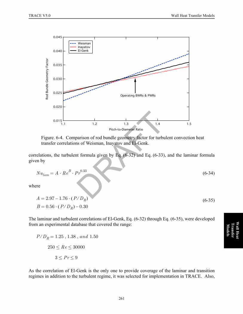
TRACE V5.0 Wall Heat Transfer Models FOOBAR1234FOOBAR1234FOOBAR1234FOOBAR1234FOOBAR1234
Wall H
eat T
ransfer M
odels
correlations, the turbulent formula given by Eq. (6-32) and Eq. (6-33), and the laminar formulagiven by
(6-34)
where
(6-35)
The laminar and turbulent correlations of El-Genk, Eq. (6-32) through Eq. (6-35), were developedfrom an experimental database that covered the range:
As the correlation of El-Genk is the only one to provide coverage of the laminar and transitionregimes in addition to the turbulent regime, it was selected for implementation in TRACE. Also,
Figure. 6-4. Comparison of rod bundle geometry factor for turbulent convection heat transfer correlations of Weisman, Inayatov and El-Genk.
! "
#$ % &
Nulam A ReB Pr0.33··=
A 2.97 1.76 P DR⁄( )
B 0.56 P DR⁄( ) 0.30–·=
·–=
P DR⁄ 1.25 1.38 and 1.50, ,=
250 Re 30000≤≤
3 Pr 9≤≤
DRAFT
261

Wall Heat Transfer Models TRACE V5.0
for the turbulent correlation, the variable property effect of Hufschmidt & Burck (Ref. 6-6) forheat transfer to liquid is included as proposed by Inayatov. Thus,
(6-36)
One potential problem with the laminar correlation of El-Genk is that it goes to zero as theReynolds no. decreases rather than approaching the expected constant value. Consequently, theanalytical results presented by Kim & Li (Ref. 6-11) for fully developed laminar flow in a rodbundle with constant heat flux boundary condition are used as a lower limit. Kim & Li presentedtheir results in a tabular format as shown in Table 6-1.
Rather than use tabular interpolation, their results are implemented in TRACE as a curvefit over
the region, , by
(6-37)
which gives a value of 6.825 for a pitch-to-diameter ratio of 1.33.
To ensure continuity, the Nusselt no. for forced convection to liquid in a rod bundle geometry istaken as the maximum of the three values given by the analytical lower limit of Kim & Li, and thelaminar and turbulent correlations of El-Genk. That is,
Table 6-1. Fully developed laminar Nusselt no. for square array rod bundles, Kim & Li (Ref. 6-11).
Pitch-to-Diameter Nusselt no.
1.02 1.618
1.10 2.845
1.2 4.600
1.3 6.377
1.5 9.448
1.8 12.99
2 15.06
Nuturb CEG Re0.8 Pr0.33 PrPrw----------
⎝ ⎠⎜ ⎟⎛ ⎞
0.11
···=
1.1 P DR⁄ 2≤ ≤
NuKL 5.6605PDR--------
⎝ ⎠⎜ ⎟⎛ ⎞
2
31.061PDR--------
⎝ ⎠⎜ ⎟⎛ ⎞
24.473–·+·–=
DRAFT
262
TRACE V5.0 Wall Heat Transfer Models FOOBAR1234FOOBAR1234FOOBAR1234FOOBAR1234FOOBAR1234
Wall H
eat T
ransfer M
odels
(6-38)
The resulting model for forced convective heat transfer in a rod bundle is compared to that for atube in Figure 6-5. In the fully turbulent regime, the rod bundle Nusselt no. is about 12% greaterthan that for a tube. However, in the laminar regime, the results are drastically different. Finally,recall that the correlations of El-Genk and the analytical result of Kim & Li are both for bare rodbundles. Thus, any heat transfer enhancement due to the presence of spacer grids should besuperposed upon this.
Similar to the heat transfer model for convection to single-phase liquid in tubes, the Nusselt no.for liquid convection in a rod bundle is taken as the maximum of the values for forced and naturalconvection. That is,
(6-39)
For the Nusselt no. due to natural convection, , TRACE needs a "local condition" modelthat correlates the wall heat transfer in terms of the local wall-to-fluid temperature difference.Most natural convection heat transfer models, however, use either an isothermal condition for theentire heat transfer surface or a constant power boundary condition and neither of these boundaryconditions is appropriate for our application.
One local-condition correlation for natural convection in vertical tubes was found in the literature[Sarma et al., (Ref. 6-12)] and was implemented in TRACE. Sarma's correlation was developedexpressly for mixed convection and is given by
(6-40)
where the Grashof no. is defined in terms of the tube diameter using Eq. (6-17). As was the casefor heat transfer in tubes, the liquid density is evaluated at the reference film temperature but allother properties are at the bulk liquid temperature. The values for the natural convection Nusseltno. from Eq. (6-40) are approximately three times higher than those for a vertical flat plate.
Two-Phase Forced Convection
As illustrated in Figure 6-2, the two-phase forced convection heat transfer regime is invokedwhenever the fluid is two-phase and the wall temperature is below that necessary for the onset of
nucleate boiling. Thus, it occurs both for fluid heating, , and for condensing
NuFC Max NuKL Nulam Nuturb,,⎩ ⎭⎨ ⎬⎧ ⎫
=
Nu Max NuFC NuNC,⎩ ⎭⎨ ⎬⎧ ⎫
=
NuNC
NuNC 0.7 GrD Prl·( )1 4⁄
·=
TONB Tw Tl> >
DRAFT
263

Wall Heat Transfer Models TRACE V5.0
flows, . In addition, as explained in the section Nucleate Boiling, the models presentedbelow for two-phase convective heat transfer are also used for the forced convection evaporationcomponent when boiling is occurring.
When the fluid condition is two-phase and forced convection heat transfer is occurring, eitherwith or without the presence of nucleate boiling, the forced convection heat transfer issignificantly enhanced above that for single-phase flow. The approach developed here will be touse the single-phase heat transfer correlations described above with an appropriate multiplier toaccount for two-phase effects.
In TRAC-PF1/MOD2, this two-phase enhancement was accounted for by using the flow factor ofthe Chen nucleate boiling correlation (Ref. 6-13). The wall-liquid forced convection heat transfercoefficient is given by
(6-41)
The first part of the above equation is recognizable as the Dittus-Boelter correlation, the last termis Chen's flow factor. The flow factor, or "F factor", is a function of the Martinelli parameter,defined by
Figure. 6-5. Comparison of models for forced convection heat transfer in tube and rod bundle geometries.
! " # $
%
&'
Tw Tsv<
hFC 2Φ,
0.023klDh------- Rel
0.8 Prl0.4 F··· ·=
DRAFT
264

TRACE V5.0 Wall Heat Transfer Models FOOBAR1234FOOBAR1234FOOBAR1234FOOBAR1234FOOBAR1234
Wall H
eat T
ransfer M
odels
(6-42)
The ratio involving the flow quality in can vary significantly from time-step to time-step forlow flow conditions where the flow quality is ill-defined. This was one of the root causes ofoscillations in RELAP5 for AP-600 calculations due to its usage in both the flow factor (whichcan vary by two orders of magnitude) and in the suppression factor of the nucleate boilingcomponent of the Chen correlation. Consequently, another approach, one that is less likely togenerate unphysical oscillations was selected for TRACE. That is, the two-phase multiplier forconvective heat transfer should be a function of the void fraction rather than of flow quality.
Recently, Kim et al. (Ref. 6-14) critically reviewed twenty different heat transfer correlations fortwo-phase forced convection by comparing them against seven sets of experimental data. Two ofthe correlations consistently recommended were those of Aggour (Ref. 6-15) and Rezkallah &Sims (Ref. 6-16). Both of these correlations have their two-phase enhancement factor based onthe void fraction and hence would be suitable for our application.
The correlation of Aggour (Ref. 6-15) is given by
(6-43)
for laminar flow, and by
(6-44)
for turbulent flow in tubes with the liquid Reynolds no. defined by
(6-45)
Xtt1 x–
x-----------
⎝ ⎠⎜ ⎟⎛ ⎞
0.9 ρgρl-----
⎝ ⎠⎜ ⎟⎛ ⎞
0.5 µlµg-----
⎝ ⎠⎜ ⎟⎛ ⎞
0.1
· ·=
Xtt
h2Φhl
-------- 1 α–( )13---–
=
Nul 1.615 Rel PrlDhL
-------··⎝ ⎠⎜ ⎟⎛ ⎞
13---µbµw------
⎝ ⎠⎜ ⎟⎛ ⎞
0.14
· ·=
h2Φhl
-------- 1 α–( ) 0.83–=
Nul 0.0155 Rel0.83 Prl
0.5 µbµw------
⎝ ⎠⎜ ⎟⎛ ⎞
0.33
···=
RelGl Dh·µl
-----------------ρl 1 α–( ) Vl Dh· · ·
µl-------------------------------------------------= =
DRAFT
265

Wall Heat Transfer Models TRACE V5.0
In both the above formulations, it is apparent that the role of the two-phase multiplier is to simplycorrect the liquid Reynolds no. so that it is based on the actual liquid velocity rather than thesuperficial liquid velocity. This is in accordance with Collier's (Ref. 6-17) observation that:
"It would appear that in the bubbly and slug flow regimes, the mechanism of heat transfer is by the normal convective process to the liquid phase and that the enhancement over the single-phase liquid heat transfer coefficient is due, in general, to the increase in the liquid phase velocity in the two-phase case."
For turbulent flow, Rezkallah and Sims (Ref. 6-16) found that an excellent method of correlatingthe two-phase convective heat transfer coefficient was what they termed the "Liquid-AccelerationModel." In this model, it is implied that the role of the gas phase is to accelerate the liquid phasewhile the heat transfer coefficient is predicted using a conventional single-phase correlation withthe liquid properties and an adjusted liquid velocity. The equation describing this model is
(6-46)
where the is the exponent on the Reynolds no. for single-phase heat transfer.
Again, it is seen that the primary role of the enhancement factor is to correct the liquid Reynoldsno. so that it is based on the actual liquid velocity rather than the superficial liquid velocity.Therefore, for implementation in TRACE, this is accomplished by defining a two-phase Reynoldsno. as
(6-47)
and using it in the evaluation of the forced convection Nusselt no. This approach should workreasonably well (and is certainly simple) for turbulent forced convection in tubes, and for bothlaminar and turbulent convection in rod bundles using the correlations given in Single-PhaseLiquid Convection, above.
For laminar convection in tubes, where the Nusselt no. is not a function of the Reynolds no., thisapproach is not applicable. For the bubbly flow and slug regimes, as per Collier's observation, itis probably sufficient to simply leave the laminar Nusselt no. unmodified and that is the case inthe TRACE model.
However, for annular flow, it is obvious that the characteristic length that should be used with theNusselt no. is not the tube diameter but rather the thickness of the annular film. This is theapproach followed in TRACE, and the heat transfer models used for convection in the annularflow regime are detailed below in Film Condensation. To ensure continuity between the two-phase convection models and those for the annular flow regime, a simple linear interpolation invoid fraction is used between the values of 80% to 90%. Specifically,
h2Φhl
-------- 1 α–( ) n–=
n
Re2ΦGl Dh·
1 α–( ) µl·---------------------------
ρl Vl Dh· ·µl
--------------------------= =
DRAFT
266
TRACE V5.0 Wall Heat Transfer Models FOOBAR1234FOOBAR1234FOOBAR1234FOOBAR1234FOOBAR1234
Wall H
eat T
ransfer M
odels
(6-48)
where the weighting factor for annular flow is given by
(6-49)
and is limited to values between zero and unity.
Onset of Nucleate Boiling
As the wall temperature increases above the saturation temperature corresponding to the totalpressure, nucleate boiling heat transfer can be initiated if the wall superheat is sufficient toactivate nucleation sites present on the surface. The wall surface temperature at which nucleateboiling heat transfer begins is denoted as the "temperature for the onset of nucleate boiling",TONB. This temperature is used as part of the heat transfer regime selection logic as depicted inFigure 6-2 for the pre-CHF heat transfer regimes.
Recently, Basu et al. (Ref. 6-18) have proposed a correlation for , the wall superheat atthe onset of nucleate boiling, that includes the effects of material surface properties by expressingthe available cavity size as a function of the fluid-surface contact angle. Included in the databasefor this model is a 9-rod bundle with Zircaloy-4 cladding.
The wall superheat is then
(6-50)
where the available cavity size, , is given by
(6-51)
with being a correction factor that depends on contact angle, and is the cavity diametercorresponding to the tangency condition. From the available data, the contact angle correctionfactor was determined to be
(6-52)
hwl wfann hann 1 wfann–( ) h2Φ·+·=
wfannα 0.8–( )0.9 0.8–( )
--------------------------=
∆TONB
∆TONB4 σ Tsat· ·
Dc ρv hfg· ·----------------------------=
Dc
Dc F φ( ) Dc0·=
F φ( ) Dc0
F φ( ) 1 φ3– 0.5 φ·–( )exp–=
DRAFT
267
Wall Heat Transfer Models TRACE V5.0
where the contact angle, , is measured in radians. is obtained by invoking the minimumsuperheat criteria as
(6-53)
Combining these equations, the wall superheat at the onset of nucleate boiling is then
(6-54)
Figure 6-6 compares the values for the wall superheat at the onset of nucleate boiling calculatedusing the model of Basu et al. (Ref. 6-18) [Eq. (6-54)] with that of the empirical correlation ofBergles & Rohsenow (Ref. 6-19) and with that of the analytical model of Davis & Anderson (Ref.6-20) for two different heat flux levels. At the modest wall heat flux level,
, the values given by all three models are nearly identical. For the higher
heat flux level, , such as might be encountered in subcooled boiling athigh flow conditions, there is a small difference between the predicted values with those given bythe models of Basu et al. being the highest and those of Bergles & Rohsenow the lowest.However, the maximum difference, that occurs at low pressure, is only about 1 Kelvin degree.
From the above comparison, any one of these models would be suitable, however, only the modelof Basu et al. (Ref. 6-18) includes the surface material effect. Consequently, it was selected foruse in TRACE. An example of the dependence upon the surface material is given in Figure 6-7which compares the values for stainless steel with those for Zircaloy-4.
Equation (6-54) is an implicit relationship as the wall heat flux, appearing on the right-hand-side,is a function of . As the value of is needed for the determination of the heattransfer regime, and an implicit formula would require an iterative solution, a procedure totranslate this implicit formula into an explicit one was developed as detailed below.
Prior to the onset of nucleate boiling, single-phase heat transfer prevails on the heater surface.Thus, the associated wall heat flux can be expressed in terms of the single-phase convective heattransfer coefficient as
(6-55)
where is the forced convection heat transfer coefficient, and
φ Dc0
Dc0 8 σ Tsat kl· · ·
ρv hfg qw″· ·-----------------------------------
⎝ ⎠⎜ ⎟⎜ ⎟⎛ ⎞
12---
=
∆TONB2
F φ( )------------
σ Tsat q″ONB· ·
ρv hfg kl· ·---------------------------------------
⎝ ⎠⎜ ⎟⎜ ⎟⎛ ⎞
12---
·=
q″ONB 105 W m2⁄( )=
q″ONB 106 W m2⁄( )=
∆TONB TONB
q″ONB hFC TONB Tl–( )· hFC ∆TONB ∆Tsub+( )·= =
hFC
DRAFT
268

TRACE V5.0 Wall Heat Transfer Models FOOBAR1234FOOBAR1234FOOBAR1234FOOBAR1234FOOBAR1234
Wall H
eat T
ransfer M
odels
Substitute Eq. (6-54) into Eq. (6-55) to yield,
(6-56)
Equation (6-56) is implicit in but can be solved using the quadratic equation as
(6-57)
where to simplify the notation, the quantity, , the wall superheat necessary for the
onset of nucleate boiling when the liquid is at saturation, has been introduced and is given by
Figure. 6-6. Comparison of wall superheat values at the onset of nucleate boiling for three different models for water-stainless steel.
!"#$ % &
'( ) *+
'( ) *+
∆TONB TONB Tsat–=
∆Tsub Tsat Tl–=
q″ONB2 hFC·F φ( )
---------------------σ Tsat q″ONB· ·
ρv hfg kl· ·---------------------------------------
⎝ ⎠⎜ ⎟⎜ ⎟⎛ ⎞
12---
hFC ∆Tsub·+·=
q″ONB
q″ONB12--- hFC ∆T
ONB sat,· hFC ∆T
ONB sat,4 hFC ∆Tsub· ·+·+⎝ ⎠
⎛ ⎞·2
=
∆TONB sat,
DRAFT
269

Wall Heat Transfer Models TRACE V5.0
(6-58)
which yields
(6-59)
The wall-liquid temperature difference is then
(6-60)
and finally
Figure. 6-7. Comparison of wall superheat values at the onset of nucleate boiling for stainless steel and Zircalloy-4 using the model of Basu et al. (Ref. 6-18) with water as the working fluid.
! " #$%&
∆TONB sat,
2F φ( )------------
σ Tsat hFC ∆TONB sat,
· · ·
ρv hfg kl· ·-------------------------------------------------------------------
⎝ ⎠⎜ ⎟⎜ ⎟⎜ ⎟⎛ ⎞
12---
·=
∆TONB sat,
2 hFC·
F 2 φ( )-----------------
σ Tsat·
ρv hfg kl· ·-------------------------·=
Tw Tl–q″ONBhFC
---------------- 14--- ∆T
ONB sat,∆T
ONB sat,4 ∆Tsub·++⎝ ⎠
⎛ ⎞ 2·= =
DRAFT
270

TRACE V5.0 Wall Heat Transfer Models FOOBAR1234FOOBAR1234FOOBAR1234FOOBAR1234FOOBAR1234
Wall H
eat T
ransfer M
odels
(6-61)
This formula for will be used to determine whether or not the heat transfer regime isforced convection or nucleate boiling. To use this model, we need the contact angle for theparticular surface-fluid combination. From Basu et al., the contact angle for water and stainlesssteel is ~38º and for water and zircaloy-4 it is ~57º. At present, TRACE uses the value forstainless steel. A future code update will introduce the effect of surface material upon .
Nucleate Boiling
The model for nucleate boiling must be suitable for pool boiling and for flow boiling at bothsaturated and subcooled conditions. The model traditionally selected for this, and the one used inTRAC-PF1/MOD2, is the Chen correlation (Ref. 6-21). The Chen correlation is a straightforwardlinear superposition of forced convection and pool boiling heat transfer components
(6-62)
where F is the flow factor discussed in Two-Phase Forced Convection above and S is thesuppression factor1.
As noted above, the flow factor is a function of the Martinelli parameter that in turn is a functionof the flow quality. The suppression factor is likewise a function of the Martinelli parameter andserves to turn off the nucleate boiling component of the wall heat flux as the flow qualityincreases. Consequently, for low flow conditions where the flow quality is ill-defined, the heattransfer coefficients calculated by the Chen correlation can vary wildly from time-step to time-step producing unphysical oscillations in the numerical solution. Although there are numerousmore modern nucleate boiling heat transfer correlations that claim higher accuracy, the Chencorrelation might be accurate enough for our purposes, however, the potential for poor numericalbehavior led to its replacement in the TRACE code.
A second reason for choosing a more modern nucleate boiling correlation is the dependency ofthe boiling heat flux upon the wall superheat. That is,
(6-63)
1. It would be preferable to use the subscript "FB" to indicate flow boiling instead of "NB". However, to avoid confusion with film boiling, "NB" will be used to indicate flow boiling.
TONB Tl14--- ∆T
ONB sat,∆T
ONB sat,4 ∆Tsub·++
⎝ ⎠⎜ ⎟⎛ ⎞
2
·+=
TONB
TONB
hNB F hFC S hPB·+·=
q″PB ∆Tsatn∝
DRAFT
271

Wall Heat Transfer Models TRACE V5.0
where the exponent is generally agreed upon to have a value between 3 and 4 (e.g., McAdams(Ref. 6-29)). However, for the Chen correlation, the value of is only about 2. For a comparisonwith other correlations, both modern and classical, refer to Table 6-2.
Also, to minimize the potential for unphysical oscillations caused by large fluctuations in theforced convective component that are especially troublesome for the low-pressure, low-flowconditions prevalent in passive plants during the long-term cooling phase, the model for the two-phase multiplier should be void fraction based rather than a function of flow quality.Consequently, the model discussed above in Two-Phase Forced Convection is retained for theforced convection component of the flow boiling regime.
Then, to complete the model for flow boiling, we need to:
1) Identify a suitable superposition method for the forced convection and nucleate boil-ing components.
2) Select a heat transfer correlation for the nucleate boiling component.
3) Determine an appropriate form for the nucleate boiling suppression factor.
4) Ensure continuity in the wall heat flux at the onset of nucleate boiling.
Each of these four items is discussed in the subsections below. Following this is a subsection onthe implementation of the selected pool boiling model.
Table 6-2. Comparison of wall superheat exponent in nucleate boiling.
CorrelationYear
Published
Pressure (bar)
2.7 70
Chen (Ref. 6-21) 1963 2.16 2.07
Cooper (Ref. 6-22) 1984 3.03 3.03
Gorenflo (Ref. 6-23) 1993 3.92 2.84
Jens-Lottes (Ref. 6-24) 1951 4 4
Levy (Ref. 6-25) 1959 - 3
McAdams (Ref. 6-26) 1949 3.96 -
Steiner & Taborek (Ref. 6-27) 1992 3.31 2.67
Thom (Ref. 6-28) 1965 2 2
nn
DRAFT
272

TRACE V5.0 Wall Heat Transfer Models FOOBAR1234FOOBAR1234FOOBAR1234FOOBAR1234FOOBAR1234
Wall H
eat T
ransfer M
odels
Flow Boiling Additive Approach
The super-position method is treated first. Steiner and Taborek (Ref. 6-27) proposed a flowboiling correlation where each of the components (forced convection and nucleate boiling) werecorrelated independently. The superposition method was an "asymptotic" or "power-type"addition model of the type proposed by Kutateladze (Ref. 6-30) and formalized by Churchill (Ref.6-31) to represent the transition between two regimes, each dominated by different limitingphenomena. In generalized form, the asymptotic addition method for flow boiling is
(6-64)
From a regression analysis using the Karlsruhe heat transfer databank, Steiner and Taborek
determined that the value of the exponent, , should be so that is the value that will be usedhere. Thus,
(6-65)
However, as we intend to use this model for both saturated and subcooled boiling where the sinktemperatures are different, the asymptotic addition method will be applied to the heat fluxcomponents rather than to the heat transfer coefficients. That is,
(6-66)
and the wall-to-liquid heat transfer coefficient becomes
(6-67)
Pool Boiling Model
To select a heat transfer correlation for the nucleate boiling component, three of the more modernboiling correlations were investigated: Steiner & Taborek (Ref. 6-27), Cooper (Ref. 6-22) andGorenflo (Ref. 6-23). As a large nucleate boiling database was not readily available, thecandidate correlations were evaluated through comparison with each other and with well-knownclassical models. For saturated pool boiling conditions, these three models were evaluated atpressures of 2.7 bar (typical of reflood and passive cooling conditions) and 70 bar (typical ofBWR operating conditions and PWR SBLOCA pressure) and compared to the McAdam's
hNB hFCn S hPB·( )
n+
1n---
=
n 3≈
hNB hFC3 S hPB·( )
3+
13---
=
q″NB q″FC3 q″PB
3+
13---
=
hwlq″NB
Tw Tl–( )------------------------=
DRAFT
273

Wall Heat Transfer Models TRACE V5.0
correlation (low pressure) and the Levy correlation (high pressure) as recommended by Holman(Ref. 6-32). The results of these comparisons are given in Figure 6-8 and Figure 6-9 where thenucleate boiling component of the Chen correlation has been included.
For low pressure conditions, all of the modern correlations predict larger values of the saturatedpool boiling heat flux than the correlation of McAdams. The model of Gorenflo has a similarslope to that of McAdams, that is, its dependence upon wall superheat has approximately thesame power (3.92 versus 3.96), while the models of both Cooper and Steiner & Taborek haveshallower slopes (exponents of 3.03 and 3.31 respectively). At high pressure conditions, themodels of Gorenflo and Cooper give values of the wall heat flux very close to that of Levy whilethe values given by Steiner & Taborek are clearly too low. The dependence upon the wallsuperheat has an exponent of 3 for Levy's correlation, 2.67 for Steiner & Taborek, 3.03 forCooper, and 2.84 for Gorenflo. Based on these comparisons, the model of Steiner & Taborek waseliminated from consideration.
Based on these comparisons, no definitive conclusions can be made as to the superiority of onecorrelation over another for the models of Cooper and Gorenflo. Also, implementationcomplexity is about the same for both models. Therefore, the model of Gorenflo was selectedbecause of its lower predicted value of the nucleate boiling heat transfer coefficient at lowsuperheats for low pressure conditions. The rationale for this choice is that during refloodsimulations, for the region below the quench front where the boiling component should simply beremoving the decay heat and wall superheats are only a few degrees, the model of Gorenflo willbe less likely to produce large wall heat flux variations in response to small pressure oscillations.
Figure. 6-8. Comparison of pool boiling correlations at low pressure.
!"#$%&'
(&& ) * +
DRAFT
274

TRACE V5.0 Wall Heat Transfer Models FOOBAR1234FOOBAR1234FOOBAR1234FOOBAR1234FOOBAR1234
Wall H
eat T
ransfer M
odels
The pool boiling model of Gorenflo uses a reference point formulation and is given by
(6-68)
where, for water,
(W/m2 - C)
(W/m2)
(6-69)
with being the reduced pressure,
and the surface roughness having the reference value
Figure. 6-9. Comparison of pool boiling correlations at high pressure.
!"#$%
&'' ( )
hPB h0 FP q″ q″0⁄( )n
RP RP0⁄( )0.133
· · ·=
h0 5600=
q″0 20000=
FP 1.73 Pr0.27 6.1 0.68
1 Pr–---------------+
⎝ ⎠⎜ ⎟⎛ ⎞
Pr2·+·=
n 0.9 0.3 Pr0.15·–=
Pr
PrP
Pcrit-----------=
DRAFT
275

Wall Heat Transfer Models TRACE V5.0
For boiling surfaces that have not been characterized, it is recommended that the roughness betaken to be , so that the surface roughness term is unity and this is the approach used inTRACE.
Nucleate Boiling Suppression Factor
The role of the nucleate boiling suppression factor is to "turn off" the nucleate boiling heat fluxcomponent as the flow regime becomes annular and the heat transfer regime switches to forcedconvection evaporation. That is, as the annular film becomes thin, the heat transfer modebecomes convection through the film causing evaporation at the interface rather than nucleation atthe wall. The suppression factor, due to its dependence upon the film thickness, is also usuallycorrelated in terms of the Martinelli parameter. Consequently, the numerical problemsencountered for the "F factor" at low flow conditions also occur for the suppression factor.
A number of recent flow boiling models, see Steiner & Taborek (Ref. 6-27) or Bjorge et al. (Ref.6-33), omit the suppression factor. Indeed, the appendix to Steiner & Taborek's paper makes theargument that the suppression factor doesn't exist. To avoid the numerical difficulties at low flowconditions observed with the Chen correlation, the approach used here will follow that which doesnot provide an explicit suppression factor. While an explicit suppression factor has not beenincluded in the TRACE model, the effect of the two-phase forced convection heat transfercoefficient upon provides an implicit suppression of the nucleate boiling component ofthe wall heat flux.
Continuity at the Onset of Nucleate Boiling
The power-law combination used for the super-position of the forced convection and the nucleateboiling heat transfer components, that is,
(6-66)
leads to a jump in the wall heat flux at the point of ONB as the value of abruptly changesfrom zero to a finite value. Though this discontinuity is usually small, it is best to remove it andthe approach of Bjorge et al. (Ref. 6-33) is adopted to accomplish this. Namely,
(6-70)
RP0 0.4 µm=
0.4 µm
∆TONB
q″NB q″FC3 q″PB
3+
13---
=
q″PB
q″NB q″FC q″PB q″BI–( )3+
13---
=
DRAFT
276
TRACE V5.0 Wall Heat Transfer Models FOOBAR1234FOOBAR1234FOOBAR1234FOOBAR1234FOOBAR1234
Wall H
eat T
ransfer M
odels
where is the fully developed boiling heat flux at the point of boiling initiation,
(6-71)
which forces the boiling component to be zero at . Furthermore, as noted above, thisapproach provides an implicit suppression factor. For example, as the forced convectioncomponent increases, increases, so that increases and the nucleate boilingcomponent of the total heat flux decreases.
Implementation of the Gorenflo Correlation
The Gorenflo correlation for the pool boiling heat transfer coefficient, with the roughness factortaken as unity, is
(6-72)
where the exponent is a function of pressure only. When only pool boiling is to be considered, thepool boiling heat flux is given by the implicit relationship
(6-73)
This can be expressed explicitly as
(6-74)
where the first term on the right hand side is a function of pressure and second term gives thedependence upon the wall superheat.
When the Gorenflo pool boiling correlation is used as part of a flow boiling correlation, where thetotal heat flux is given as the sum of forced convection and pool boiling components,
(6-70)
an ambiguity occurs with respect to what heat flux should be used in the evaluation of the poolboiling heat transfer coefficient. That is, should we use
(6-75)
q″Bl
q″BI q″PB TONB( )=
TONB
TONB q″BI
hPB h0 FP q″ q″0⁄( )n
· ·=
q″PB hPB Tw Tsat–( )· h0 FP q″PB q″0⁄( )n
Tw Tsat–( )··= =
q″PB h0 FP q″0n⁄·⎝ ⎠
⎛ ⎞
11 n–------------
Tw Tsat–⎝ ⎠⎛ ⎞
11 n–------------
·=
q″NB q″FC q″PB q″BI–( )3+
13---
=
hPB h0 FP q″PB q″o⁄( )n
· ·=
DRAFT
277
Wall Heat Transfer Models TRACE V5.0
or
(6-76)
where the subscript "PB" indicates the pool boiling component only and the subscript "NB"indicates the total flow boiling heat flux. If the latter expression, i.e., Eq. (6-76), is used, and thewall superheat is the independent variable, an iterative procedure is required to evaluate the poolboiling component.
Except near the point for the onset of nucleate boiling, there is very little difference between thesetwo approaches. Therefore, we have decided to use the approach that is the simplest to implementand the most computationally efficient. Thus, the pool boiling heat flux is used so that an explicitformula for the pool boiling heat transfer coefficient is
(6-77)
This completes the description of the models used for pool and flow boiling in the TRACE code.
Subcooled Boiling Model
When the wall temperature exceeds that necessary for the onset of nucleate boiling, ,
but the bulk liquid temperature is subcooled, , the wall heat transfer regime issubcooled nucleate boiling. In this regime, despite the subcooling of the liquid, significant levelsof void fraction exist and are important to calculate accurately due to their effects on reactorkinetics, gravity heads in passive plants, and two-phase friction losses.
Recall from the Interfacial Heat Transfer chapter that the mass transfer rate per unit volume due tointerfacial heat transfer is
(6-78)
with the interfacial heat transfer rates given by
(6-79)
for the liquid-side heat transfer and by
(6-80)
hPB h0 FP q″NB q″o⁄( )n
· ·=
hPB h0 FP q″0n⁄·( )
11 n–------------
Tw Tsat–( )n
1 n–------------
·=
Tw TONB>
Tl Tsv<
Γiq'''li q'''vi+hv∗ hl∗–( )
--------------------------=
q'''li hli A'''i Tl Tsv–( )· ·=
q'''vi hvi A'''i Tg Tsv–( )· ·=
DRAFT
278
TRACE V5.0 Wall Heat Transfer Models FOOBAR1234FOOBAR1234FOOBAR1234FOOBAR1234FOOBAR1234
Wall H
eat T
ransfer M
odels
for the gas-side heat transfer. With the liquid subcooled, the liquid-side heat transfer will benegative indicating the presence of condensation for the bulk flow conditions. Also, the gas-sideheat transfer is usually negligible as the gas temperature is typically close to saturation.Consequently, to provide a mechanism for the generation of vapor during subcooled boiling, aspecial source term, , the mass transfer rate per unit volume due to subcooled boiling, wasintroduced. Thus, the net mass transfer is
(6-81)
where for subcooled boiling, would represent bulk condensation and the net vaporgeneration rate at the wall. It is the role of this section to describe the models used to calculate
. The wall heat transfer coefficient in the subcooled nucleate boiling regime is calculatedusing the models described above in Nucleate Boiling and is not repeated here.
During subcooled boiling, vapor bubbles are generated at the wall due to nucleate boiling. Someof these bubbles immediately collapse due to condensation in the "near wall" region while othersdetach and become part of the bulk two-phase flow. Still other bubbles may slide along theheated surface before either condensing or growing large enough to detach. The details of thesemicro-processes are too complicated to be modeled explicitly in a reactor system analysis codesuch as TRACE. Instead, a constitutive model is provided that specifies the net vapor generationrate resulting from the competing processes of vapor generation and condensation in this nearwall region.
In the nucleate boiling regime, the wall heat flux is comprised of both forced convection and poolboiling components. The fraction of the wall heat flux that results in subcooled vapor generationonly derives from the pool boiling component as the forced convection component should onlyresult in a change in the sensible heat. Recall that the total flow boiling heat flux is given by
(6-70)
This power-law additive scheme makes it difficult to determine what the actual pool boilingcomponent is. Consequently, we will consider all of the wall heat flux in excess of forcedconvection as available to generate vapor, that is,
(6-82)
The net vapor generation rate due to subcooled boiling is then specified as a fraction of thisboiling heat flux by
Γsub
Γ Γi Γsub+=
Γi Γsub
Γsub
q″NB q″FC q″PB q″BI–( )3+
13---
=
q″PB q″NB q″FC–≈
DRAFT
279
Wall Heat Transfer Models TRACE V5.0
(6-83)
where is the fraction that results in subcooled vapor generation and is the surface areaof the heat transfer surface per unit volume.
The fraction of the boiling heat flux that results in subcooled vapor generation is taken from theLahey mechanistic subcooled boiling model (Ref. 6-34) and takes the form
(6-84)
where is the liquid enthalpy at which bubble detachment occurs.
Saha and Zuber (Ref. 6-35) give two separate formulations for based on the Peclet no.depending upon whether the subcooled boiling regime is thermally or hydrodynamicallycontrolled. At low mass fluxes, it was found that the point of net vapor generation is dependentonly on local thermal conditions, which determine the rates of vapor condensation andevaporation at the wall. To make an estimate of these two rates it was assumed that the rate ofevaporation at the wall was proportional to the wall heat flux, whereas the rate of condensationwas proportional to the local subcooling. Thus, the similarity parameter was taken to be the localNusselt number defined by
(6-85)
For high mass flux conditions, the phenomenon is hydrodynamically controlled, and theappropriate similarity parameter is the local Stanton number defined as
(6-86)
The Peclet number, which by definition is the ratio of the Nusselt number and the Stantonnumber, is then
, (6-87)
Γsubfsub q″NB q″FC–( ) A'''w· ·
hv sat,
hl–( )----------------------------------------------------------------=
fsub A'''w
fsub Max 0hl hld–( )
hl sat,
hld–( )-------------------------------,=
hld
hld
Nuq″NB Dh·
kl Tsat Tl–( )·------------------------------------=
Stq″NB
G cp l, Tsat Tl–( )· ·---------------------------------------------------=
Pe NuSt--------
G Dh cp l,· ·
kl------------------------------= =
DRAFT
280

TRACE V5.0 Wall Heat Transfer Models FOOBAR1234FOOBAR1234FOOBAR1234FOOBAR1234FOOBAR1234
Wall H
eat T
ransfer M
odels
was selected to be the correlation-independent parameter with the Stanton number as thedependent parameter. Data from 10 different sources were plotted as shown in Figure 6-10. Thetwo distinct regions can easily be identified. Up to a Peclet number of 70000, the data fall in astraight line having the slope of minus one, which implies a constant value for the local Nusseltnumber. This is the thermally controlled region. Beyond a Peclet number of 70000, the data fallon a constant Stanton number, which is referred to as the hydrodynamically controlled region.The entire correlation for the point of net vapor generation is then expressed as
(6-88)
These two formulas can be written simply as
(6-89)
where the Peclet no. is constrained to be larger than the critical value of . The Peclet no.is then
Figure. 6-10. Original database of the Saha-Zuber correlation.
Nu 455= : Pe 70000≤
St 0.0065= : Pe 70000>
hf hld–( )q″NB Dh Cp l,· ·
Pe St·----------------------------------------=
7.0 4×10
DRAFT
281

Wall Heat Transfer Models TRACE V5.0
(6-90)
or
(6-91)
and the Stanton no. has a constant value of 0.0065.
Finally, the implementation of this model can be made a bit simpler by writing the subcooledvapor generation fraction in terms of temperature rather than enthalpy. Thus,
(6-92)
and
(6-93)
where the Peclet no. is evaluated from Eq. (6-91) and the Stanton no. has a constant value of0.0065.
Critical Heat FluxThe point where the maximum heat flux occurs in the idealized boiling curve shown in Figure 6-1
will be denoted as the CHF point, , and is characterized by both the critical heatflux and the wall temperature at which it occurs. This is the point where the heat transfer regimetransitions from that where the liquid phase wets the wall (i.e., nucleate boiling), to the post-CHFregimes where liquid-wall contact is either transient (transition boiling) or non-existent (filmboiling).
In TRACE, the role of the CHF model is two-fold:
1) Determine the transition point for the heat transfer regime, and
2) Serve as the anchor point for the transition boiling wall heat flux (see Transition Boil-ing below).
Pe Max 7.0 104G Dh cp l,· ·
kl------------------------------,×=
Pe Max 7.0 104 Rel Prl·,×[ ]=
fsub Max 0Tl Tld–( )
Tsat Tld–( )-----------------------------,=
Tsat Tld–( )q″NB Dh·
Pe St·------------------------=
q″CHF TCHF,( )
DRAFT
282
TRACE V5.0 Wall Heat Transfer Models FOOBAR1234FOOBAR1234FOOBAR1234FOOBAR1234FOOBAR1234
Wall H
eat T
ransfer M
odels
To serve both these roles, the CHF model in TRACE must provide a continuous estimate of theCHF over a wide range of conditions with reasonable accuracy. This range of conditions mustextend from the high pressure, high-flow conditions typical of operating PWRs and BWRs, to thelow pressure, low-flow conditions existing after a LBLOCA or for a passive plant in the long termcooling phase.
For the analysis of anticipated transients, such as a perturbation in the core flow or inletsubcooling, the metric is the departure from nucleate boiling (DNB) margin. DNB is one of thetypes of CHF and for each fuel type there are specific DNB correlations with high accuracy. Mostof these correlations employ the boiling length concept, in which the core inlet quality or enthalpyexplicitly appears in the correlation. During many transients and postulated accidents, however,the use of boiling length correlations is not appropriate. For example, during a cold-leg-breakLOCA, the core experiences a flow reversal thereby rendering the definition of the core inletambiguous. In addition, these correlations are unsuited for general use in TRACE because theyare highly empirical with a limited range of validity, and are unreliable when extrapolated outsidetheir original database.
Therefore, for the default CHF model in TRACE the 1995 AECL-IPPE CHF look-up table (Ref.6-36) was selected. It is based on an extensive database of CHF values obtained in tubes with avertical upflow of a steam-water mixture and provides the value of the critical heat flux as afunction of the local conditions. As described below, a correction factor is included to improvethe accuracy of this table when applied to rod bundles. This look-up table allows for a reasonablyaccurate prediction of CHF based on the local flow conditions for a much wider range ofconditions than would be possible with either empirical correlations or phenomena based models.
To define the CHF point, the wall temperature at which the critical heat flux occurs must bedetermined. This is accomplished by solving the equation
(6-94)
which requires an iterative solution due to the non-linearities associated with the flow boiling heatflux as a function of wall temperature. As shown above in Figure 6-2, the critical heat fluxtemperature, , is used to determine whether the heat transfer regime is pre- or post-CHF.
Also, both and are used in the formulation for the wall heat flux in the transitionboiling regime.
For BWRs, the high-quality, high mass flux conditions may introduce memory effects that limitthe accuracy of a local condition CHF model such as the default look-up table. Therefore, as partof the consolidation of the TRAC-B code's capabilities into TRACE, two critical qualitycorrelations were implemented as well and are described below. Either of these critical qualitycorrelations can be selected by the user via input through the "ICHF" parameter in the heatstructure input. In TRACE, the role of these critical quality correlations is limited to that ofdetermining the transition point from nucleate to transition boiling. That is, if the local flowquality exceeds the value of xcrit , the heat transfer regime switches to post-CHF. For the wall
q″NB TCHF( ) q″CHF=
TCHF
q″CHF TCHF
DRAFT
283
Wall Heat Transfer Models TRACE V5.0
heat flux in the transition boiling regime, however, the CHF point calculated using the look-uptable is used.
AECL-IPPE CHF Table
Groeneveld et al. (Ref. 6-36) published an updated look-up table for CHF that was developedjointly by AECL1 Research (Canada) and IPPE2 (Russia). This method of determining the valueof the critical heat flux was selected for TRACE because of its reasonably good accuracy andwide range of applicability. The AECL-IPPE CHF table is based upon an extensive database ofCHF values obtained in tubes for a vertical upward flow of a steam-water mixture. While thedatabase covers a wide range of flow conditions, the look-up table was designed to provide CHFvalues for 8 mm tubes at discrete values of pressure, mass flux, and dryout quality. Three-dimensional linear interpolation is used to determine the CHF for conditions between tabulatedvalues and is implemented as a direct-indexing scheme to reduce the computational burdenassociated with a table look-up.
The database used to develop the AECL-IPPE look-up table contains 22,946 unique data pointscovering the following range of conditions:
(mm)
(MPa)
(kg/m2s)
Despite the large number of data points in this database, the data population density at some flowconditions remains relatively low thereby contributing to greater uncertainty, especially for lowflow conditions where CHF is very difficult to measure due to unstable flow conditions. Theresulting table was constructed to provide CHF values for 8 mm tubes at discrete values ofpressure, mass flux, and dryout quality, and includes empirical correction factors to extend thetable to other tube diameters and for rod bundles. Details of the table's derivation and accuracyare given in the original reference (Ref. 6-36) by Groeneveld and are not repeated here.Compared against the combined AECL-IPPE CHF databank, the 1995 look-up table predicts the
1. AECL: Atomic Energy of Canada Limited.2. IPPE: Institute of Power and Physics, Obninsk, Russia.
3 D 40≤ ≤
0.1 P 20≤ ≤
6 G 8000≤ ≤
0.5 x 1≤ ≤–
80 L D 2485≤⁄≤
DRAFT
284

TRACE V5.0 Wall Heat Transfer Models FOOBAR1234FOOBAR1234FOOBAR1234FOOBAR1234FOOBAR1234
Wall H
eat T
ransfer M
odels
data with overall average and root-mean-squared errors of 0.69% and 7.82% respectively. Theimplementation of the look-up table in TRACE is described below.
The value of the critical heat flux is given by
(6-95)
where is the correction factor for tube diameter, is the correction factor for rod bundlegeometry, is the correction factor for low flow conditions and is the table look-up value.
These correction factors and the procedures used to extrapolate outside the table boundaries aregiven below. In addition to the above correction factors, Groeneveld (Ref. 6-37) provides otherfactors for effects such as that of axial flux shape, heated length and grid spacers. However, thesefactors were not implemented in this version of TRACE.
The first parameter used in the table look-up is the total pressure. As the table values cover therange, (MPa) , extrapolation outside this range is seldom encountered. In TRACE,no provision is made for extrapolation to sub-atmospheric conditions; however, the procedurerecommended by Groeneveld (Ref. 6-37) is used to extrapolate to pressures above this range.Specifically, the pool boiling relationship is used, so that
(6-96)
where indicates the table look-up value at a pressure of 20 MPa. To avoidthe extra computational burden associated with the fluid property calls necessary to evaluate thelast term in Eq. (6-96), a curve-fit is used in TRACE. Thus,
(6-97)
where the non-dimensional pressure is defined by
(6-98)
q″CHF K1 K2 K8 fn P G x, , · · ·=
K1 K2K8 fn P G x, ,
0.1 P 20≤ ≤
q″CHF P G x, ,( ) q″CHF P20 G x, ,( )
ρg1 2⁄
hfg σ ∆ρ·[ ]1 4⁄
⎝ ⎠⎜ ⎟⎛ ⎞
P
ρg1 2⁄
hfg σ ∆ρ·[ ]1 4⁄
⎝ ⎠⎛ ⎞
P20
--------------------------------------------------------------·=
q″CHF P20 G x, ,( )
q″CHF P G x, ,( )
q″CHF P20 G x, ,( )---------------------------------------------- 1.546 P∗ 1.6108 P∗2 1.7818 P∗3 0.7199 P∗4·–·+·–·=
P∗ Pcrit P–Pcrit P20–--------------------------=
DRAFT
285

Wall Heat Transfer Models TRACE V5.0
The second parameter used in the table look-up is the mass flux, G. For co-current flowconditions, either upflow or downflow, the mass flux is taken to be the sum of the individualphasic liquid and gas mass fluxes as expected. However, for counter-current flow conditions, forwhich the table is not strictly applicable, the mass flux is set to that of the liquid phase alone. Thatis,
(6-99)
For mass flux values greater than the table upper limit, no extrapolation is made. The mass flux issimply set to the maximum value,
(6-100)
as recommended by Groeneveld (Ref. 6-37). Finally, for two-phase low mass flux conditions,
(kg/m2s) , the low flow correction factor, , is applied as described below.
The final parameter used in the table look-up is the quality, , defined as
(6-101)
where is the flowing mixture enthalpy given by
(6-102)
Substitution of Eq. (6-102) into Eq. (6-101) yields
(6-103)
Examination of Eq. (6-103) reveals that for co-current flow with saturated liquid, the expressionreduces to the expected value for the flow quality,
GGl Gg+ : Gl Gg·( ) 0>
Gl : Gl Gg·( ) 0≤⎩⎪⎨⎪⎧
=
G Min 8000 G,⎩ ⎭⎨ ⎬⎧ ⎫
=
400 G 100≤ ≤– K8
x
xhm h
l sat,–
hg hl sat,
–---------------------------=
hm
hmGl hl Gg hg·+·
Gl Gg+--------------------------------------=
xGgG------ G
G----
hl hl sat,
–
hg hl sat,
–-------------------------
⎝ ⎠⎜ ⎟⎜ ⎟⎛ ⎞
·+=
DRAFT
286
TRACE V5.0 Wall Heat Transfer Models FOOBAR1234FOOBAR1234FOOBAR1234FOOBAR1234FOOBAR1234
Wall H
eat T
ransfer M
odels
(6-104)
Similarly, for single-phase liquid conditions, Eq. (6-103) becomes the familiar
(6-105)
The definition of quality given by Eq. (6-101) and Eq. (6-102) is meaningless for counter-currentflow. Consequently, a "static" quality is introduced to account for this special case. The staticquality, , is calculated from the void fraction using Eq. (6-101) and a mixture enthalpygiven by
(6-106)
With both phases at saturation, this reduces to
(6-107)
This static quality is used both for counter-current flow conditions and for the special case of lowflow in the evaluation of the correction factor.
The CHF look-up table is constructed so that the CHF value for a quality of unity is set to zero.As the maximum dryout quality is 1.0, no need for extrapolation beyond this point is needed. Atthe lower end, table values for subcooled conditions are supplied for values down to a quality of
. For high-pressure conditions, it is possible for the liquid subcooling to be large enough thatthis lower bound is exceeded. For this case, a linear extrapolation is used as recommended byGroeneveld (Ref. 6-37).
The three correction factors used in TRACE are described next. First, the diameter factor, , is
(6-108)
and is based on data for a range of tube diameters from 0.62 mm to 92.4 mm. For large diametertubes, Groeneveld (Ref. 6-36) observed that the value of seems to approach a constant valueof about 0.6. Thus,
xGgG------=
xhl h
l sat,–
hg sat,
hl sat,
–-----------------------------------=
xstatic
hm1 α–( ) ρl hl α ρg hg· ·+· ·
1 α–( ) ρl α ρ· g+·------------------------------------------------------------------=
xstatic 1 11 α–( )ρlαρg( )
----------------------+⁄=
K8
0.5–
K1
K1 0.008 Dh⁄=
K1
DRAFT
287

Wall Heat Transfer Models TRACE V5.0
(6-109)
Also, Groeneveld notes that the CHF for small diameter tubes is more difficult to estimate due tothe small amount of data and that the effect of diameter on CHF is more likely to be affected byflow conditions. So, caution should be used when applying this correction factor to tubes with adiameter of less than 3 mm. This caveat has little relevance to reactor safety applications wherethe characteristic dimension is much larger than this value.
For rod bundle geometries, Groeneveld et al. (Ref. 6-38) recommend
(6-110)
where is the pitch-to-diameter ratio for the bundle, as the simplest one available and onethat exhibits the correct asymptotic trends. Furthermore, the value of K2 is constrained to be less
than unity. Thus, for a typical rod bundle with , the ratio of the CHF value for the
rod bundle to that of an 8 mm diameter tube is within the range . In theevaluation of this rod bundle correction factor, note that the quality is limited to positive valuesand that the diameter factor, , is set to unity.
For two-phase low mass flux conditions, Eq. (6-95) includes a correction factor denoted as .Although indicated as a multiplicative correction factor, the low flow correction is actuallyimplemented through an interpolation procedure. First, the procedure used to construct the poolboiling, G = 0 , part of the look-up table is briefly described, followed by an explanation of therecommended interpolation procedure that was implemented in TRACE.
Due to the scarcity of reliable CHF data for low flow conditions, Groeneveld (Ref. 6-36) used thepool boiling CHF model of Zuber (Ref. 6-39) as the basis for the table values at zero mass flux.Two modifications were then made to improve the accuracy of the pool boiling CHF model forsubcooled and two-phase conditions. For subcooled pool boiling, the increase in the CHF withsubcooling was modeled using the correlation of Ivey & Morris (Ref. 6-40). For negative valuesof the quality, the CHF table was then computed from
(6-111)
where is the CHF value from the Zuber pool boiling model and
K1 Max 0.6 0.008 Dh⁄,⎩ ⎭⎨ ⎬⎧ ⎫
=
K2 2PDR--------
⎝ ⎠⎜ ⎟⎛ ⎞
1.5–· x1 3⁄
2----------–
⎝ ⎠⎜ ⎟⎛ ⎞
exp·=
P DR⁄( )
P DR⁄ 1.33=
0.7339 K2 1≤ ≤
K1
K8
q″CHF P( G, 0 x 0 )<, q″CHF P G 0= x 0=, ,( ) 1 B ∆Tsub·+[ ]·= =
q″CHF P G 0= x 0=, ,( )
DRAFT
288

TRACE V5.0 Wall Heat Transfer Models FOOBAR1234FOOBAR1234FOOBAR1234FOOBAR1234FOOBAR1234
Wall H
eat T
ransfer M
odels
(6-112)
For low flow two-phase conditions, Griffith (Ref. 6-41) showed that the value of the pool boilingCHF decreased in an approximately linear manner with the decrease in the liquid fraction. Thisapproach was built into the CHF look-up table with the provision that the value of the quality usedfor the table look-up be computed using the static value given above in Eq. (6-107). Thus,
(6-113)
The mass flux boundaries of the low flow region for the AECL-IPPE CHF look-up table are
defined as (kg/m2-s). Within this region, a linear extrapolation is performedbetween the look-up table value at the limit and the pool boiling value with the quality set to the
static value. For positive flow, (kg/m2-s), this gives
(6-114)
where the weighting factor is
(6-115)
and for negative flow, ,
(6-116)
with the weighting factor given by
(6-117)
In addition to providing a much wider range of applicability than that of the Biasi CHF correlation(Ref. 6-42), the default model in the TRAC-PF1/MOD2 code, the selection of the AECL-IPPElook-up table for TRACE also provides gains in accuracy. Figure 6-11 and Figure 6-12 showexamples of the behavior of the predicted CHF values from the look-up table and from the Biasicorrelation for high-pressure high-flow case and a low-pressure low-flow case respectively.
B 0.1ρlρg-----
⎝ ⎠⎜ ⎟⎛ ⎞
0.75 cP l,
hfg----------
⎝ ⎠⎜ ⎟⎛ ⎞
·=
q″CHF P( G, 0 x 0 )>, q″CHF P( G, 0 xstatic ),== =
400 G 100≤ ≤–
0 G 100<≤
q″CHF P G x, ,( ) wf q″CHF P( G,· 100 x )
1 wf–( ) q″CHF P( G,·+
,
0 xstatic ),
= =
=
wf G 100⁄=
400 G 0 kg m2s⁄( )<≤–
q″CHF P G x, ,( ) wf q″CHF P( G,· 400 x )
1 wf–( ) q″CHF P( G,·+
,
0 xstatic ),
= =
=
wf G 400⁄–=
DRAFT
289

Wall Heat Transfer Models TRACE V5.0
Figure. 6-11. Comparison of the AECL-IPPE CHF table and the Biasi correlation for high-pressure high-flow conditions.
Figure. 6-12. Comparison of the AECL-IPPE CHF table and the Biasi correlation for low-pressure low-flow conditions.
!"#$$! % &' ( ) )*
$ + ,$
- + .(
/ +
!"#$$! % &' ( ) )*
$ + ,$
- + .(
/ +
DRAFT
290

TRACE V5.0 Wall Heat Transfer Models FOOBAR1234FOOBAR1234FOOBAR1234FOOBAR1234FOOBAR1234
Wall H
eat T
ransfer M
odels
From these figures, the applicability of the CHF table to subcooled conditions, whereas the Biasicorrelation is limited to two-phase conditions, is readily apparent. Also, in Figure 6-11, the CHFvalues for the high-pressure high-flow comparison are remarkably similar, as is to be expected, asthe database used to develop the Biasi correlation is included in that used for the lookup table.Conversely, in Figure 6-12, the CHF values for the low-pressure low-flow comparison are quitedifferent. Indeed, comparing the two figures reveals that the predicted CHF values from the Biasicorrelation for the low-pressure low-flow case exceed those for the high-pressure high-flow case.This low-flow behavior of the Biasi correlation is contrary to experimental evidence and reveals alimitation of the correlation even though these conditions are within its stated range ofapplicability.
In both Figure 6-11 and Figure 6-12, the curves of CHF versus quality from the look-up table arenot smooth. Groeneveld (Ref. 6-36) notes that this undesirable behavior is present in all threeparametric directions: pressure, mass flux, and quality. These fluctuations are attributed to datascatter, systematic differences between different data sets, and possible effects of such second-order parameters as the heated length, surface conditions and flow instability. Future revisions tothe CHF look-up table, in addition to improving accuracy, may also improve the smoothingalgorithm used to create the table.
Finally, a quantitative comparison of the accuracy of the CHF look-up table versus the Biasicorrelation is given in Reference (Ref. 6-36). The database used was that of AECL-IPPE but onlythe data points within the recommended range of the Biasi correlation were used in thecomparison. This reduced the number of data values from 22,946 to 14,977. For this reduceddata set, the overall average and RMS errors for the look-up table were 0.38% and 8.17%respectively, compared to errors of 6.48% and 14.38% for the Biasi correlation.
In summary, the wider range of applicability and improved accuracy of the AECL-IPPE look-uptable over that of the Biasi correlation led to its selection as the default model in the TRACE code.However, as stated above, for transient DNB analysis, where the flow conditions do not deviatedrastically from their nominal values, highly accurate DNB correlations for specific fuel types areavailable and should be used when the estimation of the DNB margin is paramount. Such fueltype specific DNB correlations have not been incorporated in TRACE due to their limited rangeof applicability and their proprietary nature.
For BWR conditions, as part of the consolidation of TRAC-B's capabilities within the TRACEcode, a pair of critical quality correlations were implemented in TRACE and are described in thefollowing two sections. The user, through the heat structure input "ICHF" parameter, can selecteither of these critical quality correlations. When one of these critical quality correlations isselected, its value is used in determining the transition point from pre- to post-CHF heat transferas illustrated in Figure 6-19 below. However, even in this case, the values of the CHF point,
, used in the determination of the wall heat flux for the transition boiling regimeare calculated using the CHF look-up table.q″CHF TCHF,( )
DRAFT
291
Wall Heat Transfer Models TRACE V5.0
CISE-GE Critical Quality
In a boiling water reactor, the core exit under normal operating conditions is in the annular/mistflow regime. Consequently, the transition from flow boiling to post-CHF heat transfer isgoverned by annular film dryout. The dryout of the liquid film on the wall is determined by abalance between losses due to vaporization and entrainment and gains due to droplet deposition.In future versions of TRACE, a droplet field will be included and these processes can be modeleddirectly. However, in the present two-fluid version, it is necessary to provide a constitutive modelto predict the location of film dryout and hence the point of boiling transition.
The most widely used empirical approach for the computation of the dryout point is the "criticalquality-boiling length" approach. The inclusion of the boiling length - the axial distance from thelocation where the bulk fluid enthalpy reaches saturation to the dryout point - in this approachgives a measure of the upstream history that is important to the prediction of film dryout that isnot available in a local conditions approach such as the AECL-IPPE look-up table. Two criticalquality correlations were available in the TRAC-B code and have been incorporated into TRACEas part of the code consolidation process: the CISE-GE correlation (the subject of this section),and a model derived from the Biasi CHF correlation (the subject of the next section). Either ofthese models may be selected through the specification of the "ICHF" parameter in the heatstructure input.
The critical quality-boiling length approach was introduced by Bertoletti et al. (Ref. 6-43) and hasthe general form
(6-118)
where is the boiling length and
The CISE-GE correlation (Ref. 6-44) is a modified form of the original CISE (Ref. 6-43) tubecorrelation that was derived from blowdown heat transfer experiments performed by the GeneralElectric Corporation (GE). It is therefore based on data from rod bundle experiments andincludes the effect of local peaking factors. The database from which it was derived is limited and
the correlation is adequate only for mass fluxes in the range (kg/m2-s) . Notethat in its TRACE implementation, the critical quality is set to unity if the mass flux is outside thisrange or if the boiling length is less than one meter.
xcritA LB·B LB+-----------------=
LB
A fn P G,⎩ ⎭⎨ ⎬⎧ ⎫
=
B fn P G D, ,⎩ ⎭⎨ ⎬⎧ ⎫
=
300 G 1400≤ ≤
DRAFT
292

TRACE V5.0 Wall Heat Transfer Models FOOBAR1234FOOBAR1234FOOBAR1234FOOBAR1234FOOBAR1234
Wall H
eat T
ransfer M
odels
In TRACE, the modified CISE-GE correlation from TRAC-BF1/MOD1 (Ref. 6-44) is used, sothat
(6-119)
where the last term is a correction factor for the effect of the radial peaking factor, . In the
formulas given below, the functions and are expressed in British units, specifically, themass flux has the units (Mlbm/ft2/hr), the pressure is in psia, and the boiling length in inches.Then,
(6-120)
and
(6-121)
Also, for the case of an 8x8 rod bundle,
(6-122)
which corrects for the effect of the difference between the heated perimeter for the 8x8 bundleversus a 7x7 bundle for which the correlation was originally derived.
Biasi Critical Quality
In addition to the CISE-GE critical quality correlation, a form of the Biasi CHF correlation (Ref.6-42) transformed into a critical quality correlation has been included. Phillips et al. (Ref. 6-45)developed this correlation and it was selected for inclusion in TRAC-B due to its large database
and greater mass flux range, i.e., (kg/m2s) .
The original Biasi CHF correlation has two separate formulas for the CHF value. Consequently,the transformed critical quality correlation also has two formulas for the critical quality and themaximum value of the two is used. Thus,
(6-123)
xcritA LB·B LB+----------------- 1.24
Rf----------
⎝ ⎠⎜ ⎟⎛ ⎞
·=
Rf
A B
A 1.055 0.013 P 600–400
-------------------⎝ ⎠⎜ ⎟⎛ ⎞
2
– 1.233 G 0.907 G2 0.285 G3·–·+·–=
B 17.98 78.873 G 35.464 G2·–· ·+=
B B 1.12⁄=
100 G 6000≤ ≤
xcrit Max xcrit 1,
xcrit 2,
,⎩ ⎭⎨ ⎬⎧ ⎫
=
DRAFT
293

Wall Heat Transfer Models TRACE V5.0
The general form of the Biasi critical quality correlation is
(6-124)
where the subscript k indicates the formula, is the heated perimeter, and is the wetted
perimeter. The functions and are then specified for each formula as
(6-125)
and
(6-126)
The functions of pressure, and , used in the above formulas are written in terms ofthe pressure in bars and are given by
(6-127)
The Biasi critical quality correlation was implemented the TRAC-B code due to its largerdatabase and greater mass flux range compared to the CISE-GE correlation. However, unlike theCISE-GE correlation, it is not based on rod bundle data and is also subject to the assumptionsused in converting it from a local CHF correlation into a critical quality correlation (Ref. 6-45).The TRAC-B code manual notes that the Biasi correlation gives larger values of the criticalquality than the CISE-GE correlation. An example of this is given in Figure 6-13. The over-prediction of the Biasi correlation vis-à-vis CISE-GE is considerable and indicates that the Biasiform should be used with caution due to its potential for non-conservatism.
In its TRACE implementation, due to poor performance at low mass fluxes, the Biasi
correlation is only evaluated for mass fluxes greater than 300 (kg/m2-s) . For values of the mass
xcrit k,
Ak LB·Bk LB+--------------------
PhPw-------
⎝ ⎠⎜ ⎟⎛ ⎞ 1
Rf-----
⎝ ⎠⎜ ⎟⎛ ⎞ 1 2⁄
· ·=
Ph Pw
A B
A1 1.0=
B11.048 10 8– G1.6 Dh
1.4 hfg· · ·×H P( )
--------------------------------------------------------------------------=
A2 F P( ) G1 6⁄
⁄=
B2 5.707 10 8– G7 6⁄
·× Dh1 4⁄
hfg· ·=
F P( ) H P( )
F P( ) 0.7249 0.099 P 0.032 P·– exp· ·+=
H P( ) 1.159– 0.149 P 0.019 P·– 8.99 P·
10 P2+( )------------------------+exp· ·+=
xcrit
xcrit
DRAFT
294

TRACE V5.0 Wall Heat Transfer Models FOOBAR1234FOOBAR1234FOOBAR1234FOOBAR1234FOOBAR1234
Wall H
eat T
ransfer M
odels
flux less than this, or if the boiling length is less than one meter, the critical quality is set to unity.Also, negative mass fluxes (i.e., downflow) are computed using the absolute value of the massflux.
Minimum Film Boiling TemperatureThe temperature where the minimum post-CHF heat flux occurs in the idealized boiling curveshown in Figure 6-1 will be denoted as the minimum film boiling temperature, i.e., . In theliterature, this point is referred to by many other names according to the specific circumstancesunder which it is observed. For example, during the high-pressure high-flow conditionsassociated with blowdown during a LBLOCA, it is referred to as the "rewet temperature", duringlow-pressure bottom reflood as the "quench temperature", during quenching of a rod by a fallingliquid film as the "sputtering temperature", and, of course, classically as the "Leidenfrost point".For all of these cases, this temperature designates the point at which the heat transfer regimeswitches from transition boiling to film boiling or vice-versa and corresponds to the point atwhich the wall superheat is high enough that no appreciable liquid-wall contact occurs. Thissection describes the model selected for this transition temperature. In what follows, Tmin will beused in lieu of the other names mentioned above with the one exception that a distinction will bedrawn between and the "quench temperature" as discussed below.
Figure. 6-13. Comparison of predicted critical quality for the CISE-GE and Biasi correlations for high-pressure high-flow conditions.
!" #
$% &'& ( )
*## (' + ,-!#
.## + /
Tmin
Tmin
DRAFT
295

Wall Heat Transfer Models TRACE V5.0
There is a general consensus that is governed by hydrodynamic stability for low pressureconditions and then by the maximum liquid superheat condition as the pressure increases. Ifhydrodynamic stability governs (e.g., the well-known Berenson model (Ref. 6-46)), then liquidsubcooling is an important parameter. Material properties (e.g., thermal conductivity) of theheater surface have little impact as the surface is insulated from the liquid by a relatively thickvapor film. Surface roughness, if sufficiently rough, can be a factor though, as the vapor filmmust blanket the highest peaks on the surface.
At higher pressures (perhaps as low as 2-3 bar for water), the governing process appears to switchto that of the maximum liquid superheat condition. Basically, this states that for liquid-wallcontact to occur the wall temperature must be low enough that the liquid will not exceed itsmaximum superheat value, that is the liquid temperature must remain below that at whichhomogeneous nucleation would occur. When transient conduction effects are considered, ineffect taking the instantaneous "contact temperature" to be equal to the homogeneous nucleationtemperature, then material property effects can be included and are substantial for a surface with asufficiently thick coating of a low conductivity material such as zircaloy dioxide.
Indeed, in early reactor system analysis codes such as COBRA-TRAC (Ref. 6-47) the model for used the minimum of the values given by the Berenson model and the homogeneous
nucleation temperature with a contact temperature correction applied. These two models areplotted in Figure 6-14 against data from both the Winfrith (Ref. 6-48) and Groeneveld-Stewart(Ref. 6-49) "hot patch" film boiling tests. Also included in this figure is the correlation ofGroeneveld and Stewart (Ref. 6-49). The conditions of these tests were such that subcooling wasnegligible and, as the tubes were Inconel, the contact temperature correction is also minimal.Furthermore, the tests were conducted so that the reported is more representative of a"spontaneous collapse" of film boiling rather than the "quench temperature" associated with apropagating quench front.
As can be seen in Figure 6-14, the Berenson model, which is based on hydrodynamic stability ofthe vapor film, is close to the data at only very low pressure (2 bar or less) and rapidly goes tounrealistically high values as the pressure increases. Obviously, the approach of taking theminimum of the values given by the Berenson model and the homogeneous nucleationtemperature with a contact temperature correction provides a more reasonable approximation for
over the entire pressure range than using Berenson alone. However, compared to the data,
it appears that this approach could over-predict for pressures of a few bar and under-predictit significantly for higher pressures. In addition, this approach does not capture the subcoolingeffect evident in other data.
The Groeneveld-Stewart correlation (Ref. 6-49) is an empirical relation for the minimum filmboiling temperature valid over a wide range of pressure (1-90 bar) that includes the subcoolingeffect and consequently was selected as the model for in TRACE. This correlation is basedon vapor film collapse data that is purported to be unaffected by a propagating quench front. Thereason that this distinction is made is that the "quench temperature" is somewhat higher than the
Tmin
Tmin
Tmin
Tmin
Tmin
Tmin
DRAFT
296

TRACE V5.0 Wall Heat Transfer Models FOOBAR1234FOOBAR1234FOOBAR1234FOOBAR1234FOOBAR1234
Wall H
eat T
ransfer M
odels
actual minimum film boiling temperature due to the axial conduction effects present at a quenchfront. The Groeneveld-Stewart correlation for saturated water (or positive quality conditions) isgiven by
(6-128)
for pressures less than 9 MPa where is in K and is in MPa. In their database, both
the effects of mass flux and quality (for positive values) were deemed negligible.
A significant effect of subcooling was observed and was correlated by
(6-129)
where is the subcooled quality. This can be rewritten in terms of liquid enthalpy as
(6-130)
Figure. 6-14. Comparison of data and models for the minimum film temperature for saturated water and Inconel surface as a function of pressure.
!"#$%&
' #" !"#$%& #"() * + , -
%#
Tmin sat,
557.85 44.1 P 3.72 P2·–·+=
Tmin sat,
P
Tmin Tmin sat,
x 104·
2.82 1.22 P·+( )-----------------------------------------–=
x
Tmin Tmin sat,
hl sat,
hl–⎝ ⎠⎛ ⎞
hfg------------------------------- 104
2.82 1.22 P·+( )-----------------------------------------·+=
DRAFT
297

Wall Heat Transfer Models TRACE V5.0
For pressures in excess of this correlation's database, the authors recommend that becalculated by
(6-131)
where is the wall superheat corresponding to at a system pressure of 9
MPa. The effect of Eq. (6-131) is to ramp the calculated value for to the criticaltemperature as the pressure approaches the critical point.
In Figure 6-14, the Groeneveld-Stewart correlation was plotted against both their own data andthe Winfrith data and gave a more reasonable behavior with pressure than the approach that usedBerenson and the homogeneous nucleation temperature. The inclusion of the Winfrith data in thisfigure, which were not part of the database used to develop the correlation, serves to verify itspredicted behavior for with pressure and support its selection for TRACE.
In many simple film boiling experiments, it has been observed that the minimum film boilingtemperature is greatly increased as the liquid subcooling increases. For example, Dhir andPurohit (Ref. 6-50), for subcooled forced convection film boiling on spheres in water atatmospheric pressure, observed that increased about 80 K for every 10 degree K increase inliquid subcooling. They further observed that the effects of liquid mass flux and surface materialproperties were minimal. Note, however, that their experiment was at low pressure and so shouldbe controlled by hydrodynamic stability and that the materials they tested (steel, copper, andsilver) all had relatively high thermal conductivities. The subcooling effect of the Groeneveld-Stewart correlation is in good agreement with this trend at atmospheric pressure, namely, it givesan increase of about 63 K for every 10 degree K increase in liquid subcooling.
At high pressure, it is expected that will be governed by the maximum superheat limit ofthe liquid and that subcooling would not be a major factor. Yet, the subcooling effect given bythe Groeneveld-Stewart correlation for high-pressure conditions is still considerable. Forexample, at a pressure of 9 MPa, the Groeneveld-Stewart correlation predicts an increase in of about 28 K for every 10 degree K increase in liquid subcooling. This result is somewhatsurprising as the controlling mechanism is no longer that of hydrodynamic stability. However,this trend is well supported by their database as shown in Figure 6-15 for a pressure of 9 MPa.
Figure 6-14 compared the behavior of the Groeneveld-Stewart correlation with pressure for dataassociated with the vapor film collapse mechanism up to values of 9 MPa for the system pressure.To examine its behavior both at higher pressures and for quench conditions, the high-pressurequench data taken at the ROSA-TPTF facility (a 5x5 rod bundle, (Ref. 6-51)) and for a single-rodreflood experiment conducted by JAERI (Ref. 6-52) will be used. For both series of tests, the
Tmin
Tmin ∆Tmin 9MPa( )Pcrit P–( )
Pcrit 9–( )-------------------------- Tsat+·=
∆Tmin 9MPa( ) Tmin
Tmin
Tmin
Tmin
Tmin
Tmin
DRAFT
298

TRACE V5.0 Wall Heat Transfer Models FOOBAR1234FOOBAR1234FOOBAR1234FOOBAR1234FOOBAR1234
Wall H
eat T
ransfer M
odels
liquid inlet was saturated, so no subcooling effect is present. Also, for both experiments, theheater rods were clad with Inconel 600, so material property effects, due for example to thepresence of a low-conductivity surface oxide, are expected to be minimal. However, both of theseexperiments were quenching tests and it is expected that the observed value of the quenchtemperature would be somewhat in excess of due to the aforementioned effects of axialconduction at the quench front. Given this expectation, Groeneveld-Stewart does a reasonablejob of predicting the behavior of the data with pressure as shown in Figure 6-16.
In Figure 6-16, each data point represents the mean value for all of the thermocouples in the rodbundle (9 instrumented rods with a total of about 57 thermocouples per test). The errors bars inthe figure then represent the range of measured quench temperatures, that is, the maximum andminimum observed values, for each test. The first observation from this data is that, in agreementwith the Groeneveld-Stewart correlation, there is no effect of the mass flux upon the quenchtemperature. Second, it is clear that the value of from the Groeneveld-Stewart correlationconsistently under-predicts the high-pressure quench data by 20 to 70 degrees K. Finally, thoughthe general prediction of the behavior with respect to pressure is reasonably good, theextrapolation procedure employed for pressures above 9 MPa leads to a discontinuity in the slope.It appears that the relatively rapid decrease in given by Groeneveld-Stewart for pressuresgreater than about 6 MPa is primarily a result of the data fitting procedure used and the limitationsof their database.
Figure. 6-15. Comparison of the subcooling effect in the Groeneveld-Stewart correlation with high-pressure data.
!
Tmin
Tmin
Tmin
DRAFT
299
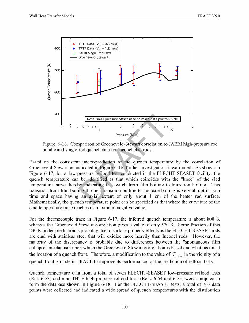
Wall Heat Transfer Models TRACE V5.0
Based on the consistent under-prediction of the quench temperature by the correlation ofGroeneveld-Stewart as indicated in Figure 6-16, further investigation is warranted. As shown inFigure 6-17, for a low-pressure reflood test conducted in the FLECHT-SEASET facility, thequench temperature can be identified as that which coincides with the "knee" of the cladtemperature curve thereby indicating the switch from film boiling to transition boiling. Thistransition from film boiling through transition boiling to nucleate boiling is very abrupt in bothtime and space having an axial extent of only about 1 cm of the heater rod surface.Mathematically, the quench temperature point can be specified as that where the curvature of theclad temperature trace reaches its maximum negative value.
For the thermocouple trace in Figure 6-17, the inferred quench temperature is about 800 Kwhereas the Groeneveld-Stewart correlation gives a value of only 570 K. Some fraction of this230 K under-prediction is probably due to surface property effects as the FLECHT-SEASET rodsare clad with stainless steel that will oxidize more heavily than Inconel rods. However, themajority of the discrepancy is probably due to differences between the "spontaneous filmcollapse" mechanism upon which the Groeneveld-Stewart correlation is based and what occurs atthe location of a quench front. Therefore, a modification to the value of in the vicinity of aquench front is made in TRACE to improve its performance for the prediction of reflood tests.
Quench temperature data from a total of seven FLECHT-SEASET low-pressure reflood tests(Ref. 6-53) and nine THTF high-pressure reflood tests (Refs. 6-54 and 6-55) were compiled toform the database shown in Figure 6-18. For the FLECHT-SEASET tests, a total of 763 datapoints were collected and indicated a wide spread of quench temperatures with the distribution
Figure. 6-16. Comparison of Groeneveld-Stewart correlation to JAERI high-pressure rod bundle and single-rod quench data for inconel clad rods.
! " #
! " #
$%&'( ) *+ ',-
.,/+-0)1
2,3 ++ ,44 - , 5 - , / 6+"
Tmin
DRAFT
300
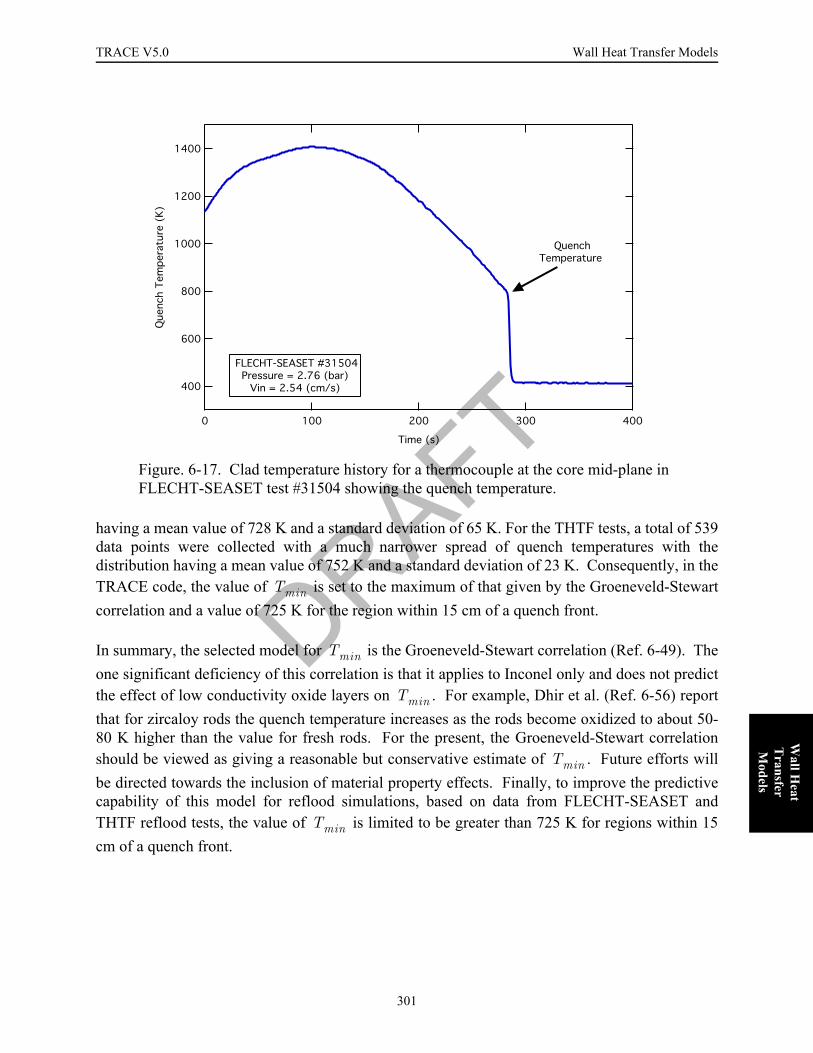
TRACE V5.0 Wall Heat Transfer Models FOOBAR1234FOOBAR1234FOOBAR1234FOOBAR1234FOOBAR1234
Wall H
eat T
ransfer M
odels
having a mean value of 728 K and a standard deviation of 65 K. For the THTF tests, a total of 539data points were collected with a much narrower spread of quench temperatures with thedistribution having a mean value of 752 K and a standard deviation of 23 K. Consequently, in theTRACE code, the value of is set to the maximum of that given by the Groeneveld-Stewartcorrelation and a value of 725 K for the region within 15 cm of a quench front.
In summary, the selected model for is the Groeneveld-Stewart correlation (Ref. 6-49). Theone significant deficiency of this correlation is that it applies to Inconel only and does not predictthe effect of low conductivity oxide layers on . For example, Dhir et al. (Ref. 6-56) reportthat for zircaloy rods the quench temperature increases as the rods become oxidized to about 50-80 K higher than the value for fresh rods. For the present, the Groeneveld-Stewart correlationshould be viewed as giving a reasonable but conservative estimate of . Future efforts willbe directed towards the inclusion of material property effects. Finally, to improve the predictivecapability of this model for reflood simulations, based on data from FLECHT-SEASET andTHTF reflood tests, the value of is limited to be greater than 725 K for regions within 15cm of a quench front.
Figure. 6-17. Clad temperature history for a thermocouple at the core mid-plane in FLECHT-SEASET test #31504 showing the quench temperature.
!"# $ %& '( $ %" )
Tmin
Tmin
Tmin
Tmin
Tmin
DRAFT
301

Wall Heat Transfer Models TRACE V5.0
Post-CHF Heat TransferThe post-CHF heat transfer regimes consist of transition and film boiling and are selected asillustrated in Figure 6-19 below. The transition boiling regime literally provides a "transition"from the wet-wall heat transfer of the nucleate boiling regime to that of "dry-wall" heat transfer inthe film boiling regime. The film boiling regime models are used to describe the wall heattransfer for the "inverted" flow regimes that occur when the surface temperature is too hot for theliquid phase to contact the wall. These regimes are described in Chapter 4, Post-CHF InterfacialDrag Models and are shown schematically in Figure 4-13. Three principal inverted flow regimesare modeled in TRACE for post-CHF conditions: inverted annular, inverted slug, and dispersedflow. The heat transfer models used for each of these regimes are described in the followingsections.
Transition Boiling
The transition boiling regime provides the transition between the "wet wall" heat transfer of thenucleate boiling regime and the "dry wall" heat transfer of the film boiling regime. There aremany correlations for the transition boiling heat transfer coefficient available in the literature,however, there is no general consensus on a best correlation. Nor is there much consistencybetween different correlations. Furthermore, oscillatory behavior in some system thermal-
Figure. 6-18. Cumulative distributions for the quench temperature at both low- and high-pressure reflood conditions for stainless steel clad rods.
!
"#$%&'$('$ &)*%" %+ ,, )-*
DRAFT
302
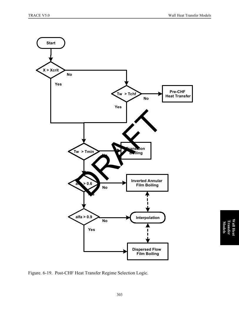
TRACE V5.0 Wall Heat Transfer Models FOOBAR1234FOOBAR1234FOOBAR1234FOOBAR1234FOOBAR1234
Wall H
eat T
ransfer M
odels
Figure. 6-19. Post-CHF Heat Transfer Regime Selection Logic.
Dispersed FlowFilm Boiling
alfa > 0.6Inverted Annular
Film BoilingNo
Yes
alfa > 0.9 InterpolationNo
Yes
X > XcritNo
Yes
Tw > Tchf
Tw > Tmin
No
Yes
Start
Pre-CHFHeat Transfer
No
TransitionBoiling
DRAFT
303

Wall Heat Transfer Models TRACE V5.0
hydraulic analysis codes has been traced to the choice of transition boiling correlation, e.g., theChen transition boiling correlation as it was implemented in RELAP5 (Ref. 6-57).
For the TRACE code, we have made the decision to use the minimum film boiling temperature asthe regime transition criteria between film boiling and transition boiling. The wall heat flux at thispoint, , is simply the film boiling heat flux calculated for the wall superheat corresponding
to . That is,
(6-132)
where the film boiling heat transfer can be either that for dispersed flow film boiling or invertedannular film boiling. For our boiling curve specification to be continuous with respect to wallsuperheat, it must pass through this minimum film boiling (MFB) point, .
Similarly, the above described CHF point, , provides the lower wall superheatboundary for the transition boiling regime. Again, for our boiling curve specification to becontinuous with respect to wall superheat, it must pass through this CHF point. Consequently,both ends of the transition boiling regime have been specified and no empirical correlation couldbe expected to match these two points. Instead, an interpolation between these two points basedon wall superheat will be implemented as the transition boiling heat transfer model.
This interpolation approach has been used with some success in the past, notably in the TRAC-PF1/MOD1 (Ref. 6-58) and COBRA/TRAC (Ref. 6-47) codes. Considering that the normalschematic representation of the boiling curve portrays the transition boiling regime as a straightline in log-log coordinates connecting the CHF and MFB points, one such scheme is logarithmicinterpolation as described in Kirchner (Ref. 6-59). The wall heat flux in the transition boilingregime would then be
(6-133)
where the exponent is calculated from
(6-134)
The resulting curve is displayed on Figure 6-20 and is denoted by the label "Log Interpolation".
A second interpolation approach is that suggested by Bjornard and Griffith (Ref. 6-60) asimplemented in both TRAC-PF1/MOD1 and COBRA/TRAC, that is
q″min
Tmin
q″min q″FB Tmin( )=
q″min Tmin,( )
q″CHF TCHF,( )
q″TB q″CHFTw
TCHF--------------
⎝ ⎠⎜ ⎟⎛ ⎞
n
·=
nq″CHF q″min⁄( )ln
TCHF Tmin⁄( )ln--------------------------------------------=
DRAFT
304

TRACE V5.0 Wall Heat Transfer Models FOOBAR1234FOOBAR1234FOOBAR1234FOOBAR1234FOOBAR1234
Wall H
eat T
ransfer M
odels
(6-135)
where
(6-136)
This formula is also displayed on Figure 6-20 and is denoted by the label "TRAC-PF1/MOD1".In effect, the interpolation weighting factor, , represents the fraction of the surfaceconsidered to have "wet-wall" heat transfer and decreases from a value of unity at the CHF pointto zero when the wall temperature reaches .
The last interpolation scheme to be considered is a cubic spline fit with the additional constraintsthat the derivative of the heat flux with respect to wall superheat is zero at both the CHF and MFBpoints. This cubic spline fit is given by
(6-137)
where
(6-138)
and
(6-139)
Figure 6-20 compares the results of all three interpolation schemes with the transition boiling dataof Johannsen et al. (Ref. 6-61) for a case with
Pressure = 2.5 (bar)Mass Flux = 50 (kg/m2-s)Inlet Subcooling = 21.7 (K)
q″TB wfTB q″CHF 1 wfTB–( ) q″min·+·=
wfTBTw Tmin–
TCHF Tmin–---------------------------------
⎝ ⎠⎜ ⎟⎛ ⎞
2
=
wfTB
Tmin
q″TB q″CHF c0 c1 θ c2 θ2 c3 θ3·+·+·+( )·=
θTw TCHF–
Tmin TCHF–---------------------------------
⎝ ⎠⎜ ⎟⎛ ⎞
=
c0 1=
c1 0=
c2 3 1( q″min q″CHF⁄ )–·–=
c323--- c2·–=
DRAFT
305

Wall Heat Transfer Models TRACE V5.0
According to their data report, the shape of the boiling curve depicted for this particular test (Run025-050-23) is representative of that observed in all of their tests.
In Figure 6-20, the CHF point is that given by the data but the MFB point is estimated based on calculated using the Groeneveld-Stewart correlation and a film boiling heat transfer
coefficient of 350 (W/m2-K) which is representative of the inverted annular film boiling regimewith a moderate subcooling. It was necessary to estimate the MFB point because it was notmeasured for the test used to obtain the transition boiling data depicted in the figure. All threeinterpolation schemes connect the CHF and MFB points as they should, however, the resultingshape of the curves are quite different.
The log interpolation scheme gives a straight line connecting the CHF and MFB points andclearly gives a poor representation of the actual boiling curve. Both the TRAC-PF1/MOD1 andthe cubic spline interpolation schemes give a reasonable approximation of the measured boilingcurve shape. No firm conclusions with respect to accuracy can be drawn due to the MFB pointbeing estimated. For example, for the same , a higher value of the wall heat transfercoefficient at the MFB point would give a higher value of and hence make the TRAC-PF1/MOD1 interpolation scheme appear to be more accurate. Conversely, a lower estimate of the wallheat transfer coefficient at the MFB point would cause the cubic spline fit appear to be moreaccurate. For TRACE, we chose the TRAC-PF1/MOD1 interpolation scheme over that of the
Figure. 6-20. Example of transition boiling interpolation schemes for Run 025-050-23 of Johannsen et al. (Ref. 6-61).
! "# $%&%' %
%% % (%%# % )% !
%%' %
Tmin
Tminq″min
DRAFT
306

TRACE V5.0 Wall Heat Transfer Models FOOBAR1234FOOBAR1234FOOBAR1234FOOBAR1234FOOBAR1234
Wall H
eat T
ransfer M
odels
cubic spline because it is simpler and should provide a slight under-estimate of the heat fluxwhereas the spline interpolation is expected to slightly over-predict.
Using the TRAC-PF1/MOD1 interpolation scheme described above, the boiling curve illustratedin Figure 6-1 was generated using the TRACE models for pre- and post-CHF heat transfer for theindicated conditions. When used in reflood simulations, this simple interpolation scheme for thetransition boiling region resulted in overly rapid quenching of the bottom portion of the heaterrod. It was found that this too rapid quenching was the consequence of the transition boiling heatflux not having a dependence upon the local value of the void fraction. Therefore, the transitionboiling weighting factor was modified to include a void fraction multiplier, namely
(6-140)
The above void fraction multiplier is an ad hoc approach to address the specific problem of toorapid quenching at the bottom of heater rods during reflood simulations. It has the undesirableconsequence of introducing a sharp decrease in the wall heat flux as the CHF point is exceeded asillustrated in the boiling curve of Figure 6-21. Also, this approach will under-predict thetransition boiling heat flux for high void fraction dispersed flow conditions such as thoseencountered at the top of a fuel rod during reflood. Consequently, during reflood simulations, thetop down quenching of the rods is expected to be under-predicted. Nevertheless, this approachhas been adopted for this first version of TRACE.
Figure. 6-21. Effect of the void fraction multiplier upon the boiling curve.
wfTB 1 α–Tw Tmin–
TCHF Tmin–---------------------------------
⎝ ⎠⎜ ⎟⎛ ⎞
2
·=
!""
DRAFT
307

Wall Heat Transfer Models TRACE V5.0
It remains to specify the heat transfer coefficients for the wall-liquid and wall-gas for thetransition boiling regime. First, the "wet wall" component of the transition boiling heat flux isassumed to be entirely transmitted to the liquid phase and is designated with a second subscript of"TB". Thus,
(6-141)
where is given by Eq. (6-140). The corresponding heat transfer coefficient is computed as
(6-142)
Also, as this "wet wall" heat flux is due to boiling heat transfer, all of it is assumed to result invapor generation. Therefore,
(6-143)
Next, the "dry wall" component of the transition boiling heat flux is calculated by evaluating theheat transfer coefficients for the film boiling regime (see below) with the wall temperature set to
. These will be designated with the addition of "FB" as a second subscript, i.e., ,
and . Finally, these "dry wall" components are weighted with the transition
boiling interpolation parameter and added to the "wet wall" components, yielding
(6-144)
The following three subsections describe the film boiling heat transfer models used for theinverted annular, dispersed flow, and inverted slug regimes. The inverted slug regime is treatedvia interpolation as indicated in Figure 6-19.
Inverted Annular Film Boiling
During film boiling, when the liquid phase is significantly subcooled, only a thin vapor filmseparates the hot surface from the subcooled liquid core. This regime is called inverted annularfilm boiling and the heat transfer paths are as depicted in Figure 6-22 below. Most of the heattransfer from the wall is across the vapor film to the saturated liquid interface. Here, part of the
q″wl TB, wfTB q″CHF·=
wfTB
hwl TB,
q″wl TB,
Tw Tl–( )------------------------
wfTB q″CHF·Tw Tl–( )
---------------------------------= =
hΓ TB,
hwl TB,
=
Tmin hwl FB,
hΓ FB,hwg FB,
hwl hwl TB,
1 wfTB–( ) hwl FB,
hΓ hΓ TB,
1 wfTB–( ) hh FB,
hwg 1 wfTB–( ) hwg FB,
·=
·+=
·+= DRAFT
308

TRACE V5.0 Wall Heat Transfer Models FOOBAR1234FOOBAR1234FOOBAR1234FOOBAR1234FOOBAR1234
Wall H
eat T
ransfer M
odels
heat is transferred into the subcooled liquid core with the remainder resulting in vapor generation.Experimental data indicate that the inverted annular regime persists up to void fractions of 60-70% and that a smooth transition is made to the dispersed flow regime. In TRACE, the invertedannular regime is assumed to exist for void fractions up to 60%. This section describes both theconvective and radiation heat transfer models used for inverted annular film boiling regime.
As indicated in Figure 6-22, the convective heat transfer between the wall and the liquid interfacehas two components: the wall-vapor and the vapor-interface heat transfer. No experimentalinformation exists as to the expected value of the vapor superheat in this regime and hence therelative magnitude of these two heat transfer resistances cannot be determined. Thus, it will beassumed that these two resistances are equal which is equivalent to assuming that the vaportemperature is halfway between that of the wall and the saturated interface.
If the vapor-liquid interface were smooth and the vapor flow laminar, then the wall heat transfercoefficient (referenced to the saturation temperature) would simply be
Figure. 6-22. Schematic of heat transfer paths for inverted annular film boiling. Vapor Liquid
Qwv Qvi Qli
TsatTv
Tw
Qrad
Tliq
DRAFT
309

Wall Heat Transfer Models TRACE V5.0
(6-145)
where is the vapor thermal conductivity and is the vapor film thickness. However, as themeasured void fraction increases, the heat transfer coefficient does not decrease as rapidly aswould be predicted by the above equation, see Figure 6-23. Considerable qualitativeexperimental evidence exists that suggests this enhancement is a result of the waviness of theinterface and/or oscillation of the liquid core thereby bringing the liquid much closer to the hotsurface than indicated by the time-averaged void fraction. Therefore, to develop an accuratemodel for heat transfer in the inverted annular film boiling regime, an empirical correction factoris needed to account for this heat transfer enhancement.
Figure 6-23 presents the low-pressure (near atmospheric) low-quality steady state film boilingdata of Fung (Ref. 6-62). This data was taken for a heated tube using the "hot patch" technique tofreeze the quench front so that steady state film boiling data could be taken. The plotted value ofthe heat transfer coefficient is referenced to the saturation temperature,
(6-146)
and has the radiative heat transfer component subtracted from it, so that
Figure. 6-23. Fung's (Ref. 6-62) low-pressure subcooled film boiling data illustrating void fraction dependence for the inverted annular film boiling regime.
hwkgδ-----=
kg δ
!"# $%
& '
& '
& '
& '
& '
& '
! ()
$%
hwq″w
Tw Tsat–( )-----------------------------=
DRAFT
310
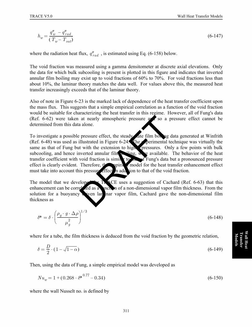
TRACE V5.0 Wall Heat Transfer Models FOOBAR1234FOOBAR1234FOOBAR1234FOOBAR1234FOOBAR1234
Wall H
eat T
ransfer M
odels
(6-147)
where the radiation heat flux, , is estimated using Eq. (6-158) below.
The void fraction was measured using a gamma densitometer at discrete axial elevations. Onlythe data for which bulk subcooling is present is plotted in this figure and indicates that invertedannular film boiling may exist up to void fractions of 60% to 70%. For void fractions less thanabout 10%, the laminar theory matches the data well. For values above this, the measured heattransfer increasingly exceeds that of the laminar theory.
Also of note in Figure 6-23 is the marked lack of dependence of the heat transfer coefficient uponthe mass flux. This suggests that a simple empirical correlation as a function of the void fractionwould be suitable for characterizing the heat transfer in this regime. However, all of Fung's data(Ref. 6-62) were taken at nearly atmospheric pressure and so a pressure effect cannot bedetermined from this data alone.
To investigate a possible pressure effect, the steady state film boiling data generated at Winfrith(Ref. 6-48) was used as illustrated in Figure 6-24. The experimental technique was virtually thesame as that of Fung but with the extension to higher pressures. Only a few points with bulksubcooling, and hence inverted annular film boiling, were available. The behavior of the heattransfer coefficient with void fraction is similar to that of Fung's data but a pronounced pressureeffect is clearly evident. Therefore, the empirical model for the heat transfer enhancement effectmust take into account this pressure effect in addition to that of the void fraction.
The model that we developed for TRACE uses a suggestion of Cachard (Ref. 6-63) that thisenhancement can be correlated as a function of a non-dimensional vapor film thickness. From thesolution for a buoyancy driven laminar vapor film, Cachard gave the non-dimensional filmthickness as
(6-148)
where for a tube, the film thickness is deduced from the void fraction by the geometric relation,
(6-149)
Then, using the data of Fung, a simple empirical model was developed as
(6-150)
where the wall Nusselt no. is defined by
hwq″w q″rad–Tw Tsat–( )
-----------------------------=
q″rad
δ∗ δρg g ∆ρ· ·
µg2
-------------------------⎝ ⎠⎜ ⎟⎛ ⎞ 1 3⁄
·=
δ D2---- 1 1 α––( )·=
Nuw 1 0.268 δ∗0.77 0.34–·( )+=
DRAFT
311

Wall Heat Transfer Models TRACE V5.0
(6-151)
and has a minimum value of unity so that it devolves into the laminar theory. In Eq. (6-150) theterm in parentheses is the enhancement factor due to the waviness or oscillatory behavior of theliquid core. Note, in developing this model, an estimate of the heat transfer due to thermalradiation [see Eq. (6-158)] was subtracted from the total heat transfer before the data wascorrelated.
In TRACE, the heat transfer rate corresponding to that of the laminar theory is represented by awall-gas component while the heat transfer enhancement is modeled as a wall-interfacecomponent. That is,
(6-152)
and
(6-153)
Figure. 6-24. Winfrith subcooled film boiling data showing pressure dependence of the heat transfer coefficient in the inverted annular film boiling regime.
!
! " #
! "
! "
! " $
Nuwhw δ·
kg-------------=
hwg 2kgδ-----·=
hΓ hwlkgδ----- Nuwl
Tw Tsat–( )Tw Tl–( )
-----------------------------··= =
DRAFT
312

TRACE V5.0 Wall Heat Transfer Models FOOBAR1234FOOBAR1234FOOBAR1234FOOBAR1234FOOBAR1234
Wall H
eat T
ransfer M
odels
where the liquid Nusselt no. is given by
(6-154)
In Eq. (6-152), the factor of 2 was added because the wall-gas heat transfer coefficient isreferenced to the gas temperature and this has been assumed to be halfway between that of thewall and the saturated interface, consistent with the model used for the interfacial heat transfer.Eq. (6-153), for the wall-liquid heat transfer coefficient, is referenced to the liquid temperature asopposed to the saturation temperature thereby necessitating the final term in this formula, which isusually not far from unity.
This simple, wholly empirical, model provides a good estimate of the wall heat transfercoefficient for Fung's subcooled data as depicted in Figure 6-25. It also does a reasonable job ofcorrelating the pressure effect observed in the Winfrith data as shown in Figure 6-26 though someunder-prediction of the high-pressure data for thick vapor films is evident.
The model for the inverted annular film boiling heat transfer enhancement given by Eq. (6-150) isstrictly only applicable to tube geometry. To investigate its possible validity to rod bundlegeometry, a database of film boiling heat transfer coefficient versus void fraction was generatedusing the forced-feed reflood data of the FLECHT-SEASET 161-Rod tests (Ref. 6-53). Toaccomplish this, at specific times in the reflood transient, axial profiles of both the heat transfer
Figure. 6-25. Comparison of TRACE empirical model for the IAFB enhancement factor versus the subcooled data of Fung (Ref. 6-62).
Nuwl Max 0 0.268 δ∗0.77 0.34–·,⎩ ⎭⎨ ⎬⎧ ⎫
=
! "! ! # $%!
& ' ()*+
, -
, -
, -
, -
, -
, -
#./ &
DRAFT
313
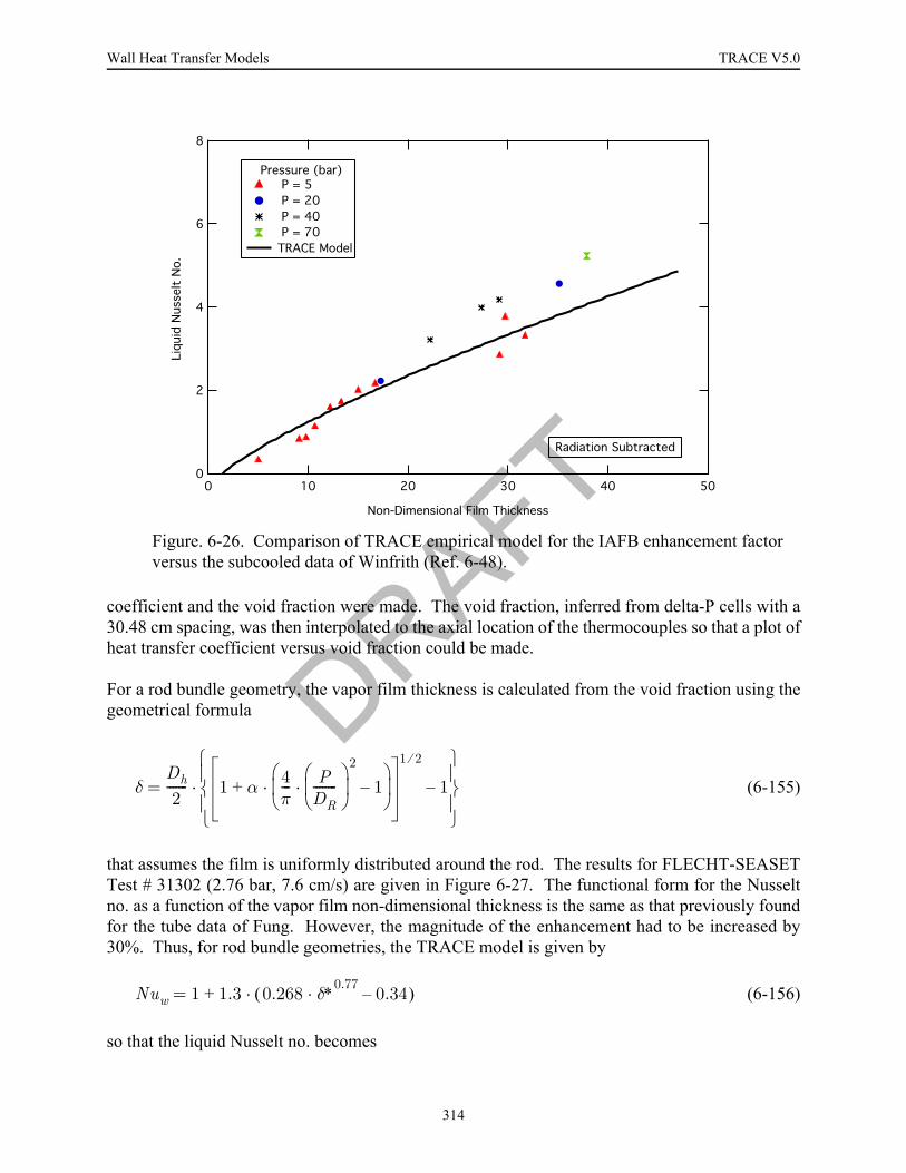
Wall Heat Transfer Models TRACE V5.0
coefficient and the void fraction were made. The void fraction, inferred from delta-P cells with a30.48 cm spacing, was then interpolated to the axial location of the thermocouples so that a plot ofheat transfer coefficient versus void fraction could be made.
For a rod bundle geometry, the vapor film thickness is calculated from the void fraction using thegeometrical formula
(6-155)
that assumes the film is uniformly distributed around the rod. The results for FLECHT-SEASETTest # 31302 (2.76 bar, 7.6 cm/s) are given in Figure 6-27. The functional form for the Nusseltno. as a function of the vapor film non-dimensional thickness is the same as that previously foundfor the tube data of Fung. However, the magnitude of the enhancement had to be increased by30%. Thus, for rod bundle geometries, the TRACE model is given by
(6-156)
so that the liquid Nusselt no. becomes
Figure. 6-26. Comparison of TRACE empirical model for the IAFB enhancement factor versus the subcooled data of Winfrith (Ref. 6-48).
!"
#" " $!"%# &
# &
# &
# & '
()* +
δDh2
------- 1 α 4π--- P
DR--------
⎝ ⎠⎜ ⎟⎛ ⎞
2
1–·⎝ ⎠⎜ ⎟⎛ ⎞
·+
1 2⁄
1–
⎩ ⎭⎪ ⎪⎨ ⎬⎪ ⎪⎧ ⎫
·=
Nuw 1 1.3 0.268 δ∗0.77 0.34–·( )·+=
DRAFT
314
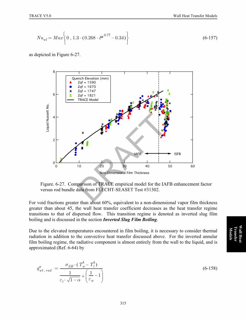
TRACE V5.0 Wall Heat Transfer Models FOOBAR1234FOOBAR1234FOOBAR1234FOOBAR1234FOOBAR1234
Wall H
eat T
ransfer M
odels
(6-157)
as depicted in Figure 6-27.
For void fractions greater than about 60%, equivalent to a non-dimensional vapor film thicknessgreater than about 45, the wall heat transfer coefficient decreases as the heat transfer regimetransitions to that of dispersed flow. This transition regime is denoted as inverted slug filmboiling and is discussed in the section Inverted Slug Film Boiling.
Due to the elevated temperatures encountered in film boiling, it is necessary to consider thermalradiation in addition to the convective heat transfer discussed above. For the inverted annularfilm boiling regime, the radiative component is almost entirely from the wall to the liquid, and isapproximated (Ref. 6-64) by
(6-158)
Figure. 6-27. Comparison of TRACE empirical model for the IAFB enhancement factor versus rod bundle data from FLECHT-SEASET Test #31302.
Nuwl Max 0 1.3 0.268 δ∗0.77 0.34–·( )·,⎩ ⎭⎨ ⎬⎧ ⎫
=
! "#$% & '
$% & (
$% & ((
$% &
)*+ ,
-*. -/.
q″wl rad,σSB Tw
4 Tl4–( )·
1εl 1 α–·------------------------- 1
εw------ 1–
⎝ ⎠⎜ ⎟⎛ ⎞
+
-----------------------------------------------------=
DRAFT
315

Wall Heat Transfer Models TRACE V5.0
where and are the liquid and the wall emissivities respectively. The radiation from thewall to the vapor phase is ignored. As the wall-liquid radiation is absorbed within the liquid, asopposed to occurring at the surface, it can be considered as a sensible heat input. The wall-liquidradiation heat transfer coefficient is then
(6-159)
and is added to that for the convective heat transfer.
In summary, the heat transfer coefficients for the inverted annular film boiling regime are
(6-152)
for the wall-gas component,
(6-160)
for the wall-liquid component, and
(6-153)
for the wall-interface heat transfer that results in subcooled vapor generation. The wall-liquidNusselt no. in Eq. (6-160) and Eq. (6-153) is given by either Eq. (6-154) for tube geometries orEq. (6-157) for rod bundles.
Dispersed Flow Film Boiling
In TRACE, the dispersed flow film boiling regime is assumed to exist for void fractions greaterthan 90%. This regime consists of a finely dispersed droplet mixture with the continuous phasebeing superheated vapor. The void fraction, especially for low-pressure conditions, is generallyin excess of 99% though the quality is often 50% or even lower. The two primary components ofthe wall heat transfer are forced convection to the superheated vapor and thermal radiation to theliquid droplets. In dispersed flow film boiling, droplet-to-wall contact heat transfer is commonlyadded to the convective heat transfer, usually through some variant of the Forslund-Rohsenowcorrelation (Ref. 6-65). However, for wall temperatures in excess of the Leidenfrost point, this
εl εw
hwl rad,
q″wl rad,
Tw Tl–( )------------------------
σSB Tw2 Tsat
2+( ) Tw Tsat+( )·
1εl 1 α–·------------------------- 1
εw------ 1–
⎝ ⎠⎜ ⎟⎛ ⎞+
-------------------------------------------------------------------------= =
hwg 2kgδ-----·=
hwlkgδ----- Nuwl
Tw Tsat–( )Tw Tl–( )
----------------------------- hwl rad,
+··=
hΓkgδ----- Nuwl
Tw Tsat–( )Tw Tl–( )
-----------------------------··= DRAFT
316

TRACE V5.0 Wall Heat Transfer Models FOOBAR1234FOOBAR1234FOOBAR1234FOOBAR1234FOOBAR1234
Wall H
eat T
ransfer M
odels
drop contact heat transfer is small compared to the uncertainty in the convective component andso it is not treated in TRACE.
The primary heat transfer mode is usually convection from the wall to the superheated steam withthe consequent level of superheat being governed by the interfacial heat transfer between thesteam and the droplet mixture. Dispersed flow film boiling is then modeled as a superposition ofradiative and convective components with the heat transfer equivalent of a two-phase multiplieron the convective term, that is
(6-161)
where
(6-162)
The two-phase enhancement factor, , accounts for the enhancement of the convectivecomponent of the wall-vapor heat transfer due to the presence of the dispersed droplets in thesuperheated vapor flow. The single-phase vapor Nusselt no., , is calculated using the
normal single-phase forced convection heat transfer correlations for the gas phase as if it wereflowing alone.
The heat transfer correlations used for the wall-gas convective heat transfer are essentially thosedescribed above in Single-Phase Liquid Convection with modifications for property anddevelopment length effects as described below. Next, the model developed for the two-phaseconvective enhancement effect is described. Finally, the radiation heat transfer models fordispersed flow film boiling are discussed.
Convective Heat Transfer Models
This section describes the models used for wall-gas convective heat transfer for single-phase andfor dispersed flow. Most of these correlations are essentially the same as those described abovefor single-phase liquid convective heat transfer with some changes to incorporate variableproperty effects for the gas and development length effects. In addition to standard models fortube geometry, models specific to rod bundle geometry are available in TRACE. Models for rodbundles are invoked for the core region of a vessel and for the fuel rods in a CHAN component.In either case, correlations are provided for the laminar and turbulent forced convection regimesand mixed convection effects are considered.
For both tubes and rod bundles, the wall heat transfer coefficient for single-phase gas convectionis taken as the maximum of the values for laminar and turbulent forced convection. That is,
q″DFFB q″wg FC, q″wl rad, q″wg rad,+ +=
q″wg FC,kgDh------- Nu
wg FC,Ψ2Φ Tw Tg–( )· ··=
Ψ2Φ
Nuwg FC,
DRAFT
317

Wall Heat Transfer Models TRACE V5.0
(6-163)
where is the wall heat transfer coefficient for laminar or mixed convection and is thewall heat transfer coefficient for turbulent forced convection
The characteristic length used for the convective heat transfer regimes is the hydraulic diameter;consequently the wall-gas heat transfer coefficient is given by
(6-164)
where the gas thermal conductivity is evaluated at the bulk fluid temperature.
The forced convection heat transfer models used for tube geometry are described first, followedby those for rod bundle geometry. For low flow conditions, the temperature differential betweenthe wall and the gas can be large enough that mixed or natural convection becomes important.TRACE also considers mixed convection effects for the laminar flow regime as detailed below inthe Mixed Convection Effects subsection.
Tube Geometry
For laminar forced convection, the Nusselt no. is set to the analytical value for fully developedflow with a constant heat flux boundary condition. Thus,
(6-6)
Laminar forced convection typically has long development lengths, however, these are notconsidered in TRACE. Instead, the fully developed laminar Nusselt no. given by Eq. (6-6) is usedas a lower limit on the wall forced convection heat transfer. Also, the effect of variable fluidproperties upon the heat transfer coefficient in laminar flow is neglected.
For turbulent forced convection, it was decided to use a modern heat transfer correlation thatwould also be applicable to the transition region. As recommended by both Bhatti and Shah (Ref.6-1) and Incropera and De Witt (Ref. 6-2), we selected the Gnielinski correlation (Ref. 6-3) forimplementation in TRACE. For fully developed turbulent flow with constant properties, theGnielinski correlation is
(6-9)
hwg Max hlam hturb,⎩ ⎭⎨ ⎬⎧ ⎫
=
hlam hturb
hwgkgDh------- Nuwg·=
Nulam 4.36=
Nuturbf 2⁄( ) Re 1000–( ) Pr·
1 12.7 f 2⁄( )1 2⁄
Pr2 3⁄
1–⎝ ⎠⎛ ⎞·+
---------------------------------------------------------------------------=
DRAFT
318

TRACE V5.0 Wall Heat Transfer Models FOOBAR1234FOOBAR1234FOOBAR1234FOOBAR1234FOOBAR1234
Wall H
eat T
ransfer M
odels
where the friction factor is evaluated using the smooth tube formula of Filonenko (Ref. 6-4), seeEq. (6-10).
The above formulation for the Nusselt no. is valid over the range
but yields negative values for Reynolds numbers less than 1000. So, the gas Reynolds no. islimited to be greater than 1000, and is defined by
(6-165)
For similar reasons, the Prandtl no. in Eq. (6-9) is constrained to have a value greater than 0.15.
The effect of variable properties upon the Nusselt no., due to the large temperature differenceacross the boundary layer, can be significant. For turbulent forced convection to a gas in a tube,Gnielinski uses the temperature ratio factor
(6-166)
which is valid for
where the subscripts and designate variable and constant properties respectively. Thistemperature ratio range is quite limited, therefore TRACE uses the variable property correctionfactor proposed by Sleicher & Rouse (Ref. 6-66), which has the form
(6-167)
where the exponent is
(6-168)
2300 Re 5 106×
0.5 Pr 2000≤≤
≤≤
Regρg Vg Dh· ·µg
----------------------------=
NuvpNucp------------
TwTg-------
⎝ ⎠⎜ ⎟⎛ ⎞
0.45–
=
0.67TwTg------- 2≤ ≤
vp cp
NuvpNucp------------
TwTg-------
⎝ ⎠⎜ ⎟⎛ ⎞
n
=
n
n Tw Tg⁄( )10log[ ]
14---
– 0.3+=
DRAFT
319

Wall Heat Transfer Models TRACE V5.0
The Sleicher & Rouse correction factor is valid for the range
which implies that the fluid is being heated. For dispersed flow film boiling during reflood,
however, there arises the possibility for the condition of reverse heat transfer, that is, .
For this case, the formula for the exponent is undefined and TRACE uses the value of -0.36initially suggested by Petukhov (Ref. 6-67) for cooling of the fluid.
In fully turbulent flow, entrance effects are generally negligible for development lengths greaterthan about 60 L/D's. However, at the moderate Reynolds nos. typical of dispersed flow filmboiling, entrance length effects can enhance the wall heat transfer by up to 15% for L/D's as largeas 50, see Figure 6-28. In a reactor system thermal-hydraulic code such as TRACE, correctionfactors for entrance effects are difficult to apply, as the "entrance" is not always clearly defined,especially in the case of reverse flow. For large break LOCA analysis, the peak clad temperatureusually occurs during the reflood phase of the transient in the dispersed flow film boiling regime.Therefore, in TRACE, a provision is made to include entrance effects for this special case, namelywhere a quench front exists, the flow is positive and the heat transfer regime is either single-phaseforced convection or dispersed flow film boiling. For this case, the entrance length is defined asthe distance downstream of the bottom quench front, i.e.,
(6-169)
Molki & Sparrow (Ref. 6-68) proposed an empirical correction factor for the entrance lengtheffect in turbulent forced convection that is a function of both the entrance length and theReynolds no., see Figure 6-28. For implementation in TRACE, we have selected the simplerformula of Bhatti & Shah (Ref. 6-1) that is only a function of the entrance length. The correlationBhatti & Shah is based on the experimental data of Mills (Ref. 6-69) for an abrupt contraction andis given by
(6-170)
where the subscript on the Nusselt no. indicates that it is the average value over thatdevelopment length. As shown in Figure 6-28, the simpler correlation of Bhatti & Shah is in goodagreement with that of Molki & Sparrow for moderate Reynolds nos. Bhatti & Shah state that this
formula is valid for ; so to stay within its database and avoid unreasonably large valuesfor this effect, the value of is constrained to be larger than 3 in TRACE.
1TwTg------- 5< <
Tw Tg<
n
LD----
Z ZQF–Dh
--------------------=
NuLNu0----------- 1 2.4254
L D⁄( )0.676
---------------------------+=
L
L D 3>⁄L D⁄
DRAFT
320

TRACE V5.0 Wall Heat Transfer Models FOOBAR1234FOOBAR1234FOOBAR1234FOOBAR1234FOOBAR1234
Wall H
eat T
ransfer M
odels
Note that although the above correction factors for variable properties and entrance length effectswere developed for tube data, they are also applied for heat transfer in rod bundles in TRACE.Likewise, the treatment for mixed convection is the same for tubes and rod bundles (as detailedbelow in the Mixed Convection Effects subsection).
Rod Bundle Geometry
Although it has been standard practice to use tube correlations for forced convection heat transferin a rod bundle, this tends to under-estimate the wall heat transfer coefficient. Consequently, itwas decided to implement heat transfer correlations specific to rod bundle geometry in TRACE asdescribed below.
As explained above in the section Single-Phase Liquid Convection, the correlation of El-Genk etal. (Ref. 6-10) provides coverage of the laminar and transition regimes in addition to the turbulentregime, and was selected for implementation in TRACE. For fully developed turbulent flow in abare rod bundle their correlation is based on that of Dittus-Boelter correlation and is given by
(6-32)
where
Figure. 6-28. Comparison of models for the entrance length effect in turbulent forced convection.
! "# $ %
Nuturb CEG Re0.8 Pr0.33··=
DRAFT
321
Wall Heat Transfer Models TRACE V5.0
(6-33)
and the fluid properties are evaluated at the bulk fluid temperature.
The effect of variable fluid properties is treated using the relation of Sleicher & Rouse (Ref. 6-66)as described above. So,
(6-171)
where the exponent is given by Eq. (6-168). Also, for turbulent convection, the entrance lengtheffect of Bhatti & Shah (Ref. 6-1) is added using Eq. (6-170).
For the transition and laminar regimes El-Genk et al. correlate the Nusselt no. by
(6-34)
where
(6-35)
As was the case for laminar convection in tubes, no correction factors for variable property orentrance length effects are applied to Eq. (6-34).
The laminar and turbulent correlations of El-Genk, Eq. (6-32) through Eq. (6-35), were developedfrom an experimental database that covered the range:
One potential problem with the laminar correlation of El-Genk is that it goes to zero as theReynolds no. decreases rather than approaching the expected constant value. Consequently, theanalytical results presented by Kim & Li (Ref. 6-11) for fully developed laminar flow in a rodbundle with constant heat flux boundary condition are used as a lower limit, see Table 6-1 andEq. (6-37). For low flow conditions, mixed convection effects can become significant and aretreated as described in the following section.
CEG 0.028 PDR--------
⎝ ⎠⎜ ⎟⎛ ⎞
0.006–·=
Nuturb CEG Reg0.8 Prg
0.33 TwTg-------⎝ ⎠
⎛ ⎞n
···=
n
Nulam A ReB Pr0.33··=
A 2.97 1.76 P DR⁄( )
B 0.56 P DR⁄( ) 0.30–·=
·–=
P DR⁄ 1.25 1.38 and 1.50, ,=
250 Re 30000≤≤
3 Pr 9≤≤
DRAFT
322

TRACE V5.0 Wall Heat Transfer Models FOOBAR1234FOOBAR1234FOOBAR1234FOOBAR1234FOOBAR1234
Wall H
eat T
ransfer M
odels
Mixed Convection Effects
When the wall-to-fluid temperature difference is large and the velocity low, the potential forbuoyancy forces to influence the heat transfer arises. For laminar flow with the buoyancy forceaiding the flow (i.e., heated upflow or cooled downflow), the resultant acceleration of the fluidnear the wall leads to an increase of the wall heat transfer coefficient. Also, according to Worsoe-Schmidt and Leppert (Ref. 6-70), when the buoyancy force acts in opposition to the flow (e.g.,heated down flow) in laminar flow, instability tends to develop at quite low values of the naturalconvection parameter and transition to turbulent flow occurs at Reynolds numbers far below theusual critical value. The result is an enhancement of the wall heat transfer above that for forcedconvection alone. So, for laminar flow, mixed convection effects always serve to increase theheat transfer coefficient.
To account for the effect of mixed convection in dispersed flow film boiling, TRACE uses thesuperposition method of Churchill (Ref. 6-31) to modify the laminar Nusselt no.,
(6-172)
The forced convection Nusselt no. for laminar flow, , is evaluated by the formulas
given above for tubes and rod bundles. For the Nusselt no. due to natural convection, ,TRACE needs a "local condition" model that correlates the wall heat transfer in terms of the localwall-to-fluid temperature difference. Most natural convection heat transfer models, however, useeither an isothermal condition for the entire heat transfer surface or a constant power boundarycondition and neither of these boundary conditions is appropriate for our application.
One local-condition correlation for natural convection in vertical tubes was proposed by Sarma etal. (Ref. 6-12) and was tested for use in TRACE. Sarma's correlation is
(6-173)
where the Grashof no. is defined in terms of the tube diameter and wall-to-fluid temperaturedifference as
(6-174)
where is the thermal expansion coefficient and is the dynamic viscosity. During simulationswith TRACE, it was found that Eq. (6-173) over-estimated the core heat transfer for low-flowconditions. Indeed, for the range of Rayleigh numbers encountered in the core during lowflooding rate reflood tests, the correlation of Sarma et al. gave values of the Nusselt no. aboutthree times larger than those calculated using the formula of McAdams (Ref. 6-71) as illustratedin Figure 6-29.
Nulam Nulam FC,3 NuNC
3+1 3⁄
=
Nulam FC,
NuNC
NuNC 0.7 GrD Prg·( )1 4⁄
·=
GrD g βg Tw Tg–( ) D3 νg2⁄· · ·=
β ν
DRAFT
323

Wall Heat Transfer Models TRACE V5.0
Consequently, the correlation of Sarma was replaced in TRACE by that of McAdams forturbulent natural convection from a vertical flat plate, given by
(6-175)
In the McAdams correlation, the length scale in the Grashof no. is the total height of the platewhereas in TRACE, the length scale is taken to be the hydraulic diameter. This discrepancy isinconsequential because when the Nusselt no. is converted to a heat transfer coefficient the lengthscale dependence is removed. That is,
(6-176)
becomes
(6-177)
Figure. 6-29. Comparison of natural convection heat transfer models for the range of Rayleigh nos. encountered in the core during low flooding rate reflood tests.
NuNC 0.13 GrL Prg·( )1 3⁄
·=
NuNC 0.13g βg Tw Tg–( ) Dh
3· · ·
νg2
------------------------------------------------------ Prg·1 3⁄
·=
hwg NC,
0.13 kgg βg Tw Tg–( )· ·
νg2
------------------------------------------ Prg·1 3⁄
· ·=
DRAFT
324
TRACE V5.0 Wall Heat Transfer Models FOOBAR1234FOOBAR1234FOOBAR1234FOOBAR1234FOOBAR1234
Wall H
eat T
ransfer M
odels
In TRACE, the natural convection Nusselt no. given by Eq. (6-176) is always added to that offorced convection for laminar flow using the superposition method of Churchill as shown inEq. (6-172). This accounts for the heat transfer enhancement evident in both buoyancy-aided andbuoyancy-opposed laminar flows.
Mixed convection effects also exist for turbulent flow conditions. As for laminar flow, buoyancy-opposed flows lead to an enhancement of heat transfer. However, for buoyancy-aided flows, ifthe buoyancy force is large enough with respect to the forced convection, the flow can "re-laminarize" with the result that the heat transfer coefficient is somewhat decreased. For TRACEapplications, e.g., reflood heat transfer, these effects are considered to be of secondary import andno mixed convection effects are considered for turbulent flow.
For stagnant flow conditions, the usage of the Nusselt no. for fully-developed laminar flow inEq. (6-172) leads to an over-prediction of the wall heat transfer. For example, the fully-developed laminar Nusselt no. is 4.36 for a tube and 6.825 for a rod bundle with a pitch-to-diameter ratio of 1.33, whereas the Nusselt no. for natural convection, appropriate for stagnationconditions, would have a value perhaps as low as 1 or 2. Consequently, a procedure to "turn off"the laminar forced convection component is needed as the flow goes to zero.
The Eckert-Metais map (Ref. 6-72), see Figure 6-30, indicates the regions of forced, mixed andnatural convection for flow in a vertical tube. The vertical axis is the Reynolds no. and thehorizontal axis is the product of the Rayleigh no. and the ratio of tube diameter to length. Thismap is valid for the range , but is not directly applicable in TRACEbecause of the usage of the tube diameter-to-length ratio that can be ambiguous during a transientsimulation. Therefore, we decided to use a procedure based on a constant value of the Richardsonno. instead of directly applying the Eckert-Metais map.
The Richardson no. is given by
(6-178)
and provides a measure of the importance of the buoyancy forces to those associated with forcedconvection. In general, buoyancy forces become non-negligible when the Richardson no. exceedsa value of unity. As the Richardson no. increases further, the effects of forced convectioneventually become negligible and the heat transfer can be modeled by free convection only.
In TRACE, we have selected a value of 100 for the Richardson no. at which only free convectionis considered. Then, a logarithmic ramp is used to gradually turn off laminar forced convection asthe Richardson no. ranges from 1 to 100. That is,
(6-179)
0.01 Pr D L⁄·( ) 1≤ ≤
RiGrD
ReD2
-----------=
wfFC100( )10 Ri( )10log–log100( )10 1( )10log–log
---------------------------------------------------------2 Ri( )10log–
2---------------------------------= =
DRAFT
325

Wall Heat Transfer Models TRACE V5.0
and
(6-180)
where the weighting factor is only evaluated for values of the Richardson no. between 1 and 100.
To relate the procedure used in TRACE to the Eckert-Metais map, two lines of constantRichardson no. were plotted in Figure 6-30. For laminar flow conditions, the mixed-freeconvection boundary line, below which only free convection is important, is reasonably wellapproximated by
(6-181)
Taking this maximum value of the Richardson no. equal to be 100 corresponds to a length-to-diameter ratio of about 40 for superheated steam. For a rod bundle in an operating PWR, the
distance between grid spacers gives an of about 44. So, the mixed-free convectionboundary for a PWR rod bundle for low-flow steam conditions is reasonably well represented bya Richardson no. of 100.
Figure. 6-30. The Eckert-Metais (Ref. 6-72) map for mixed convection in vertical tubes.
! " # #$% %
Nulam FC,
wfFC Nulam FC,
·=
Rimax2.5
Pr D L⁄( )·----------------------------=
L D⁄
DRAFT
326

TRACE V5.0 Wall Heat Transfer Models FOOBAR1234FOOBAR1234FOOBAR1234FOOBAR1234FOOBAR1234
Wall H
eat T
ransfer M
odels
Also shown in Figure 6-30 is a line for
(6-182)
that roughly corresponds to the forced-mixed convection boundary. Again, for a PWR rod bundlein low-flow steam conditions, this line is approximately equal to a Richardson no. of unity andprovides some basis for ramping the laminar forced convection Nusselt no. to zero as theRichardson no. increases from a value of 1 to 100 as given by Eq. (6-179) and Eq. (6-180).
Two-Phase Enhancement of Convective Heat Transfer
The wall-to-gas convective heat flux for dispersed flow film boiling is given by
(6-162)
where is the two-phase enhancement factor and the single-phase vapor Nusselt no.,
, is calculated using the normal single-phase forced convection heat transfer
correlations for the vapor phase as if it were flowing alone. accounts for the enhancement ofthe convective component of the wall-gas heat transfer due to the presence of the disperseddroplets in the superheated vapor flow.
An example of two-phase convective enhancement is given in Figure 6-31 as a plot of theconvective Nusselt no. versus vapor Reynolds no. for dispersed flow film boiling in a tube. Forthe data, the two-phase Nusselt no. was calculated from
(6-183)
where the gas temperature was measured but the radiative heat flux was estimated using themodels described in the section below. The curve labeled "Gnielinski" represents the single-phaseNusselt no. for turbulent forced convection calculated with a Prandtl no. of 0.91. The data shownin Figure 6-31 is highly uncertain due to the experimental difficulties encountered in performingsteady-state film boiling experiments and in measuring the temperature of the superheated steamin a dispersed flow. Nevertheless, it is apparent that as the vapor Reynolds no. decreases into thetransition region, the observed enhancement over the single-phase value increases dramatically.It is for this enhancement that a model was implemented in TRACE.
Two separate film boiling heat transfer databases were used in the model selection process. Thefirst database consists of tests from the following experiments:
•Lehigh Tube Steady State [Nijhawan, (Ref. 6-73)]
Rimin0.025
Pr D L⁄( )·----------------------------=
q″wg FC,kgDh------- Nu
wg FC,Ψ2Φ Tw Tg–( )· ··=
Ψ2Φ
Nuwg FC,
Ψ2Φ
Nuwg 2Φ,
Dhkg-------
q″meas q″rad–( )Tw Tg–( )
----------------------------------------·= DRAFT
327

Wall Heat Transfer Models TRACE V5.0
•Lehigh Tube Quasi-Steady State [Evans et al., (Ref. 6-74)]
•Winfrith Test Series 3 (Ref. 6-48)
•Harwell Mark II Experiments (Ref. 6-75)
and has a total of 301 data points. In the above tests, either a "hot patch" was used to freeze thequench front at the test section inlet or the quench front was allowed to propagate into the testsection and the data was analyzed as a series of quasi-steady axial "snapshots". For the aboveexperiments, either an aspirated steam probe or bare fluid thermocouples were used to measurethe superheated vapor temperature. As only data points where the vapor temperaturemeasurement was judged by the experimenters to be of high quality were included in thisdatabase, the resulting fluid conditions tended to be in the highly dispersed flow regime and henceat relatively high values of the flow quality. For this reason, this database will be referred to asthe "high quality" database.
The reasonably accurate measure of vapor superheat in the high quality database allowed for astraightforward calculation of the actual flow quality and derived quantities such as the vaporReynolds no. and single-phase Nusselt no. However, critical parameters such as the entrainedliquid volume fraction and droplet diameter, necessary for the development of a model for theenhancement, had to be inferred from the data using the TRACE models for drop diameter andinterfacial drag described in Chapter 4, Post-CHF Interfacial Drag Models. Consequently, theuncertainty in this database is even larger than the experimental uncertainty in quantities such asthe wall heat flux, the actual quality and the steam temperature.
Figure. 6-31. Example of two-phase convective enhancement for high-quality dispersed flow film boiling in a tube.
! " #$ %& ''
() *
+ ,-$.
+ ,/0.
1 & ,2 3 .
DRAFT
328

TRACE V5.0 Wall Heat Transfer Models FOOBAR1234FOOBAR1234FOOBAR1234FOOBAR1234FOOBAR1234
Wall H
eat T
ransfer M
odels
The second database consisted of the following experiments:
•Winfrith Test Series 3 (Ref. 6-48)
•Winfrith Test Series 4 (Ref. 6-76)
•Harwell Mark II Experiments (Ref. 6-75)
•Fung Low-Pressure Film Boiling (Ref. 6-62)
and has a total of 368 data points. All of these experiments utilized a tube test section and a hotpatch to freeze the quench front at the inlet. For these tests, the void fraction was measured by agamma densitometer at several axial elevations. These same tests were used in the developmentof the inverted annular film boiling model described above. The difference here is that only datapoints where the equilibrium quality is positive are considered (the data used in the invertedannular film boiling model development all were at subcooled conditions). The addition of thissecond database added flow conditions where significant liquid fractions existed such as areexpected for the transition region between inverted annular and dispersed flow.
However, for these liquid rich flows, it was not possible to measure the vapor temperature,therefore to back calculate the vapor heat transfer coefficient from the wall heat flux, the vaportemperature has to be inferred from the fluid conditions. This was accomplished by performing aheat balance between the imposed wall heat flux and the interfacial heat transfer with the keyassumption being that all of the wall heat flux (minus the radiative component) was assumed to betransferred to the liquid droplets via interfacial heat transfer. This assumption tended to over-estimate the vapor temperature and hence indicate higher than actual values for the two-phaseenhancement. The data points in this database tend to be at lower quality and higher liquidfraction conditions than the "high quality" database and will be referred to as the "low quality"database.
Once the local fluid conditions were inferred for both of these databases, a comparison was madebetween the experimental value of the wall heat flux and that calculated assuming single-phaseforced convection to vapor and thermal radiation. Figure 6-32 makes this comparison andillustrates the large enhancement over single-phase forced convection that results from thepresence of the liquid droplets within the vapor stream. For the high quality data, labeled as"Tvap Measured", the average value of the two-phase enhancement is ~70% while the maximumvalue is almost a factor of four times larger than the single-phase heat transfer alone. For the lowquality database, labeled as "Void Fraction Measured", the average value of the two-phaseenhancement is about 5.5 while the maximum is almost 30. The large enhancement values seenfor the low quality data are somewhat inflated due to the assumptions used in our analysisprocedure (see comment above). Nevertheless, both these results illustrate the importance ofmodeling this enhancement factor, without which significant under-predictions of the dispersedflow film boiling heat transfer are likely to occur.
Two separate mechanisms have been proposed for the heat transfer enhancement observed indispersed flow film boiling: 1) turbulence enhancement, and 2) distributed heat sinks. In the first,it is proposed that the wake turbulence caused by droplet drag increases the overall free streamturbulence level and thereby enhances the wall heat transfer. In the second, it is supposed that the
DRAFT
329

Wall Heat Transfer Models TRACE V5.0
droplets act as heat sinks distributed throughout the superheated vapor changing the radialtemperature profile and hence the heat transfer. Models from the literature based on thedistributed heat sink approach (see Refs. 6-77 and 6-78) were compared to this database butcaused large over-predictions of the heat transfer coefficient under reflood conditions.Consequently, the model chosen for TRACE is based on turbulent enhancement and wasmodified to provide a conservative estimate of the two-phase enhancement.
For the high quality database, the majority of the data points are in the dispersed flow film boilingregime and have void fractions in excess of 95%. Whereas, for the low quality database, the voidfractions range from about 70-90% and indicate that the flow regime is primarily inverted slug.Other than this obvious difference in void fraction level, the high quality data tend to be at highervalues of the vapor superficial velocity, which in turn implies that the drop diameter is smallerthan that of the low quality data. For the low quality data, the larger drops and higher dropvolume fractions would make a model based on wake induced turbulence enhancement morelikely.
Clare and Fairbairn (Ref. 6-79) proposed two similar two-phase turbulence enhancement modelsof differing complexity. Their "complex" model was compared to our database but the scatterwas unacceptably large. Their "simple" model was based on the observation that, for a roughwall, the heat transfer coefficient is approximately equal to that for a smooth wall multiplied bythe square root of the ratio of the rough-wall to smooth-wall friction factors, that is
Figure. 6-32. Comparison of calculated versus measured heat flux for dispersed flow film boiling database assuming single-phase vapor convection and thermal radiation only.
! ! "
DRAFT
330

TRACE V5.0 Wall Heat Transfer Models FOOBAR1234FOOBAR1234FOOBAR1234FOOBAR1234FOOBAR1234
Wall H
eat T
ransfer M
odels
(6-184)
Using this "rough wall" analogy, they proposed that the two-phase heat transfer coefficient couldbe represented by
(6-185)
where is an equivalent "friction factor" for two-phase dispersed flow. This equivalent two-phase friction factor was defined by
(6-186)
where is the wall drag force per unit volume and is the interfacial drag force per unitvolume given by
(6-187)
and
(6-188)
respectively.
Then, for steady dispersed flow, the interfacial drag force can be approximated by the buoyancyforce, yielding
(6-189)
The two-phase enhancement factor then becomes
(6-190)
hroughhsmooth------------------
froughfsmooth-----------------=
h2Φh1Φ--------
f2Φfw-------=
f2Φ
f2ΦDh Fw
″′ Fi″′+( )·
2 ρg Vg2· ·
-------------------------------------=
Fw″′ Fi
″′
Fw″′ fw
ρg Vg2·
2----------------- 4
Dh-------··=
Fi″′ CD
3 ρg Vrel2· ·
4---------------------------- 1 α–( )
dd-----------------· ·=
Fi″′ 1 α–( ) g ∆ρ· ·=
Ψ2Φ 11 α–( ) g ∆ρ Dh·· ·
2 fw ρg Vg2· · ·
--------------------------------------------------+1 2⁄
=
DRAFT
331

Wall Heat Transfer Models TRACE V5.0
Equation (6-190) can be rewritten in terms of a two-phase Grashof no. and the gas Reynolds no.as
(6-191)
where
(6-192)
If we assume that the wall friction factor has its fully developed value for a smooth pipe of 0.005(as suggested by Drucker et al. (Ref. 6-80)), then
. (6-193)
Equation (6-193) does a reasonable job of correlating the "low quality" data but caused the peakclad temperature in reflood simulations to be under-predicted. Therefore, the magnitude of theenhancement factor was reduced to
(6-194)
for implementation in TRACE. Also, to eliminate unreasonably large values for thisenhancement factor at low Reynolds no. conditions, is limited to have a value no greaterthan 5.
The correlating group that we have chosen is the same as that used by Kianjah et al. (Ref. 6-81) tocorrelate their heat transfer data for air-particle dispersed flows using 30 and 100 glassspheres. Their data was correlated by
(6-195)
and
Ψ2Φ 11 α–( ) Gr2Φ·
2 fw Reg2· ·
-----------------------------------+1 2⁄
=
Gr2Φρg g ∆ρ Dh
3·· ·
µg2
-------------------------------------=
Ψ2Φ 1 1001 α–( ) Gr2Φ·
Reg2
-----------------------------------·+1 2⁄
=
Ψ2Φ 1 251 α–( ) Gr2Φ·
Reg2
-----------------------------------·+1 2⁄
=
Ψ2Φ
µm
Ψ2Φ 1 71.51 α–( ) Gr2Φ·
Reg2
-----------------------------------0.85
·+=
DRAFT
332

TRACE V5.0 Wall Heat Transfer Models FOOBAR1234FOOBAR1234FOOBAR1234FOOBAR1234FOOBAR1234
Wall H
eat T
ransfer M
odels
(6-196)
for the 30 and 100 particles respectively. The TRACE model, given by Eq. (6-194),produces very similar results for the enhancement as the empirical correlation of Kianjah for a100 diameter spheres as shown in Figure 6-33. The original form of this model, as given byEq. (6-193), would produce values for the enhancement about halfway between those for the 30and 100 glass spheres.
Both of the air-particle mixtures that Kianjah et al. (Ref. 6-81) tested were mono-dispersed andthey noted a sizable particle diameter effect as evidenced by their usage of two differentcorrelations and as shown in Figure 6-33. However, for a poly-dispersed mixture containing both30 and 100 spheres, the observed heat transfer enhancement was close to that for the 30 spheres alone. The poly-dispersed result is probably more realistic for dispersed droplet flow asthe droplet diameter range covers a continuous spectrum. Consequently, the model implementedin TRACE would be expected to yield a conservative estimate of the two-phase enhancement.
The TRACE model is compared to both the high-quality (indicated by the data points labeled"Tvap Measured) and the low-quality (indicated by the data points labeled "Void Fraction
Figure. 6-33. Comparison of two-phase enhancement calculated using the TRACE model [Eq. (6-194)] to the empirical results of Kianjah et al. (Ref. 6-81) for spherical particles in air.
Ψ2Φ 1 2.6+1 α–( ) Gr2Φ·
Reg2
-----------------------------------1 2⁄
·=
µm
µm
µm
µm µm
!" #$
!" #$
# %&
# %&
DRAFT
333

Wall Heat Transfer Models TRACE V5.0
Measured) databases in Figure 6-34. As expected, the majority of the data points are under-predicted because the TRACE model was given a conservative bias to avoid under-predicting thepeak clad temperature during reflood. For the high-quality database, the wall heat flux wasunder-predicted by an average of 28% and had an RMS error of 34%. For the low-qualitydatabase, the wall heat flux was under-predicted by an average of 33% and had an RMS error of47%.
The large scatter in this comparison and the model's conservative bias, necessary for TRACEduring reflood calculations, point to inaccuracies in this modeling approach. These inaccuraciesare due to the uncertainties in the experimental data, to the larger uncertainties associated with theanalysis technique to infer local flow conditions, and to the correlation itself. Resolving this two-phase convective enhancement, in addition to improving the models for droplet diameter, isnecessary for future improvement in the code's predictive capability for dispersed flow heattransfer.
Radiation Heat Transfer Models
The final component in the model for dispersed flow film boiling heat transfer is the addition ofradiation heat transfer. Two models are provided for this: 1) the default model (described below),and 2) a radiation enclosure model (see the descriptions of the CHAN and RADENC componentsin Volume 2 of the TRACE User’s Guide, as well as Reference 6-94 for details of the actualphysical model). The radiation enclosure model includes rod-to-rod and rod-to-wall radiation
Figure. 6-34. Comparison of calculated versus measured heat flux for dispersed flow film boiling database using the TRACE model for two-phase convective enhancement.
! !"
DRAFT
334
TRACE V5.0 Wall Heat Transfer Models FOOBAR1234FOOBAR1234FOOBAR1234FOOBAR1234FOOBAR1234
Wall H
eat T
ransfer M
odels
heat transfer in addition to wall-to-fluid. This enclosure model is automatically invoked for theCHAN component (BWR fuel bundles) and can be selected as a user option for other heatstructures. The default model, however, only includes wall-fluid radiation as described below.
The default radiation model for the dispersed flow regime is that developed by Sun, Gonzalez,and Tien (Ref. 6-82). They demonstrated that if the dispersed flow regime is "optically thin", thenthe wall, vapor, and liquid droplets could be treated as single nodes in a conventional networkanalysis of radiation heat transfer. Surface-to-surface radiation is not included and theassumption that the vapor-droplet mixture is optically thin means that the liquid and vapor do notself-absorb emitted radiation. In their network model, radiation energy exchange between thewall and the droplets, the wall and the gas, and the gas and the droplets were considered. InTRACE, the gas-to-droplet radiation is not modeled as it is negligible in comparison to theinterfacial heat transfer.
The wall-to-fluid radiation heat fluxes were expressed by Sun et al. (Ref. 6-82) as
(6-197)
where and are the wall-to-liquid and wall-to-gas gray body factors respectively, and
is the Stefan-Boltzman constant ( W/m2-K). The gray body factors are
(6-198)
where
(6-199)
q″wl rad, Fwl σSB Tw4 Tsv
4–⎝ ⎠⎛ ⎞
q″wg rad, Fwg σSB Tw4 Tg
4–( )· ·=
· ·=
Fwl Fwg
σSB 5.670 8–×10
Fwl 1 R2 1R3R1------
R3R2------+ +
⎝ ⎠⎜ ⎟⎛ ⎞
⁄
Fwg 1 R1 1R3R1------
R3R2------+ +
⎝ ⎠⎜ ⎟⎛ ⎞
⁄=
=
R11 εg–
εg 1 εgεl–( )-----------------------------
R21 εl–
εl 1 εgεl–( )-----------------------------
R31
1 εgεl–( )-----------------------
1 εw–εw
---------------+=
=
=
DRAFT
335

Wall Heat Transfer Models TRACE V5.0
The emissivities for the gas and liquid droplets, and , used in Eq. (6-199) are calculated
using the method described in Reference 6-94. Both and are functions of the average beamlength and this has been taken to be equal to 0.9 times the hydraulic diameter as recommended in(Ref. 6-82). The emissivity for the wall, , would be a function of the temperature and possiblyof time as the surface undergoes oxidation. For simplicity, it is set to a fixed value of 0.7 asrecommended in the RELAP5 Manual (Ref. 6-57) for Zircaloy.
Finally, in TRACE, the wall-to-droplet heat flux is modified from that given in Eq. (6-197) to
(6-200)
This modification simplifies the necessary conversion to a heat transfer coefficient referenced tothe liquid temperature as required by the phasic energy equations. Also, when radiation heattransfer is significant, there is little difference in the values of the wall-droplet radiation heat fluxcalculated using either Eq. (6-197) or Eq. (6-200).
Inverted Slug Film Boiling
The inverted annular flow regime typically occurs when subcooled liquid flows past the quenchfront. Just downstream of the quench front, a thin vapor film separates this subcooled liquid corefrom the hot wall. The vapor velocity is low so that the flow is laminar and the gas-liquidinterface is smooth. Further downstream of the quench front, as the subcooling of the liquid coreis reduced, the vapor flow increases causing the interface to first become wavy and then oscillateviolently until breakup occurs at about the point where the liquid becomes saturated.Experimental data indicate that the inverted annular regime persists up to void fractions of 60-70% and that a smooth transition is made to the dispersed flow regime. In TRACE, the invertedannular regime is assumed to exist for void fractions up to 60%. For void fractions greater thanabout 60%, equivalent to a non-dimensional vapor film thickness greater than about 45, the wallheat transfer coefficient decreases as the heat transfer regime transitions to that of dispersed flow.This transition regime is denoted as inverted slug film boiling.
To ensure a smooth transition for the wall heat transfer coefficient between inverted annular film
boiling and dispersed flow film boiling , the TRACE model employsinterpolation as illustrated in Figure 6-35. This is accomplished by using a spline interpolationfunction to ramp the inverted annular heat transfer to zero at a void fraction of 90% and that has azero derivative at a void fraction of 60%. The wall heat transfer coefficients for the inverted slugregime are then
εg εl
εg εl
εw
q″wl rad, Fwl σSB Tw4 Tl
4–( )· ·=
α 0.6≤( ) α 0.9≥( )
DRAFT
336
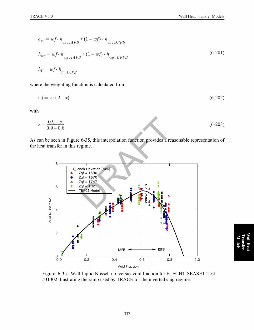
TRACE V5.0 Wall Heat Transfer Models FOOBAR1234FOOBAR1234FOOBAR1234FOOBAR1234FOOBAR1234
Wall H
eat T
ransfer M
odels
(6-201)
where the weighting function is calculated from
(6-202)
with
(6-203)
As can be seen in Figure 6-35, this interpolation function provides a reasonable representation ofthe heat transfer in this regime.
Figure. 6-35. Wall-liquid Nusselt no. versus void fraction for FLECHT-SEASET Test #31302 illustrating the ramp used by TRACE for the inverted slug regime.
hwl wf hwl IAFB,
1 wf–( ) hwl DFFB,
hwg wf hwg IAFB,
1 wf–( ) hwg DFFB,
hΓ wf hΓ IAFB,
·=
·+·=
·+·=
wf x 2 x–( )·=
x 0.9 α–0.9 0.6–---------------------=
!""#$% & '(
$% & )
$% & ))
$% &
*+, - DRAFT
337

Wall Heat Transfer Models TRACE V5.0
Condensation Heat TransferWhenever the surface temperature of a heat structure is less than the saturation temperature
corresponding to the vapor partial pressure, i.e., , condensation will occur. In TRACE,models for condensation heat transfer either with or without non-condensable gases have beenimplemented and are invoked whenever the above wall temperature criterion is met and the voidfraction is greater than 90%. As illustrated in the pre-CHF heat transfer regime selection map, seeFigure 6-2, condensation heat transfer that occurs when the void fraction is less than 80% ishandled using the normal models for two-phase convection. Also, for void fraction valuesbetween these two limits, , interpolation is used as given in Eq. (6-48) andEq. (6-49). This section describes the models that are used for the wall heat transfer coefficientwhen condensation is occurring and the void fraction is greater than 90%.
During filmwise condensation, condensation occurs at the liquid-vapor interface. As depicted inFigure 6-36, this heat transfer occurs in a two-step process, whereby heat is removed from thetwo-phase interface by interfacial heat transfer, , and then from the subcooled liquid to the
wall, . The models used by TRACE for interfacial heat transfer were previously described inChapter 5, this section describes the models used for the wall heat transfer coefficient. Theprimary mode of condensation is filmwise, and for this mode the heat transfer coefficient is thatfrom the wall to the liquid phase, , and the corresponding models are given in FilmCondensation below. However, especially during transient calculations, wall condensation canoccur when there is not enough liquid present to cover the wall with a film. For this case, it isnecessary to specify a wall-to-gas heat transfer coefficient as described in DropwiseCondensation. Finally, the section Non-Condensible Gas Effects describes the modificationsused when non-condensable gases are present.
Film Condensation
The primary mode for condensation heat transfer is filmwise as depicted above in Figure 6-36.This section describes the models used for the heat transfer coefficient between the liquid and thewall, defined by
(6-204)
where is the film thickness. One of the requirements for the TRACE condensation model wasthat it must be applicable to both falling films (such as occur on containment structures) andsheared films (e.g., high velocity flows in condenser tubes). Using the film thickness as thecharacteristic length allows for both cases as the primary effect of interfacial shear is filmthinning. Likewise, the TRACE condensation model must be applicable over a wide range of
Tw Tsv<
0.8 α 0.9< <
Qli
Qwl
hwl
hwlklδ---- Nuwl·=
δ
DRAFT
338
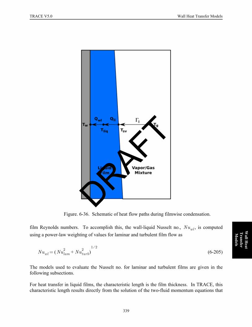
TRACE V5.0 Wall Heat Transfer Models FOOBAR1234FOOBAR1234FOOBAR1234FOOBAR1234FOOBAR1234
Wall H
eat T
ransfer M
odels
film Reynolds numbers. To accomplish this, the wall-liquid Nusselt no., , is computedusing a power-law weighting of values for laminar and turbulent film flow as
(6-205)
The models used to evaluate the Nusselt no. for laminar and turbulent films are given in thefollowing subsections.
For heat transfer in liquid films, the characteristic length is the film thickness. In TRACE, thischaracteristic length results directly from the solution of the two-fluid momentum equations that
Figure. 6-36. Schematic of heat flow paths during filmwise condensation.
Nuwl
Nuwl Nulam2 Nuturb
2+( )1 2⁄
=
DRAFT
339

Wall Heat Transfer Models TRACE V5.0
yield the void fraction as a function of wall drag, interfacial shear, and gravity. The film thicknessis then calculated from the void fraction by the formula
(6-206)
and is constrained to be greater than 10 . This limiting value was selected because a film withthat thickness gives a heat transfer coefficient of about the same magnitude as dropwisecondensation.
Laminar Film Heat Transfer
For a smooth laminar film, the Nusselt no. for heat transfer across the film1 is simply unity, sothat
(6-207)
corresponding to conduction through the film. The Reynolds no. for a film is defined by
(6-208)
where is the film flow rate per unit width of the wetted perimeter. Thus, using the definition ofthe hydraulic diameter,
(6-209)
and so the Reynolds no. is the same as that for single-phase pipe flow. As the film Reynolds no.increases above a value of about 20, (see Ref. 6-83), ripples develop on the film surface andenhance the heat transfer primarily by the film thinning that occurs in the troughs. At sufficientlyhigh Reynolds no. values, roll waves appear leading to further heat transfer enhancement.
There are many correlations in the literature to account for the wave-induced enhancement of heattransfer in laminar-wavy falling films. For example, Kutateladze (Ref. 5-8) recommended
(6-210)
1. Note that the subscript ’cond’, for condensation, will be used for heat transfer across a liquid film that includes both the wall-liquid and liquid interface heat transfer resistances.
δDh2
------- 1 α–( )·=
µm
hcondklδ----=
Ref4 Γf·µl
------------=
Γf
Ref4 Γf·µl
------------Gl Dh·µl
-----------------= =
Nucond 0.895 Ref1 12⁄
·=
DRAFT
340

TRACE V5.0 Wall Heat Transfer Models FOOBAR1234FOOBAR1234FOOBAR1234FOOBAR1234FOOBAR1234
Wall H
eat T
ransfer M
odels
However, when compared to the UCB pure steam condensation tests for cocurrent downflow in atube (Ref. 5-7), correlations such as that given by Eq. (6-210) over-predicted the datasignificantly. Therefore, the empirical correlation of Kuhn, Schrock and Peterson (Ref. 5-7)given by
(6-211)
was selected for implementation in TRACE.
The Kuhn-Schrock-Peterson (K-S-P) empirical correlation is compared to its database in Figure6-37 and to the Kutateladze model (Ref. 5-8). From the form of Eq. (6-211), it is obvious that theNusselt no. reduces to the correct value of one for conduction through a film as the film Reynoldsno. goes to zero. The enhancement as the film Reynolds no. increases is attributed to the onset ofripples though this enhancement is less than that of the Kutateladze model. From its database, the
K-S-P correlation is applicable to films with Reynolds nos. in the range: .
In its original form, the K-S-P correlation was for the Nusselt no. across a film duringcondensation and hence included heat transfer resistances for both the wall-liquid and liquid-interface. To translate it into a correlation for interfacial heat transfer, it is necessary to make anassumption regarding the apportioning of these two resistances. As, the interfacial heat transferpackage also uses the K-S-P correlation for laminar films (see Chapter 5), exactly how the
Figure. 6-37. Comparison of Kuhn-Schrock-Peterson correlation for laminar film condensation with its database.
Nucond 1 1.83 4–×10 Ref·+=
50 Ref 2000≤≤
DRAFT
341

Wall Heat Transfer Models TRACE V5.0
resistances are apportioned is of little consequence as the total heat transfer resistance will remainthe same. Consequently, it was decided to simply divide the total heat transfer resistance into twoequal parts. Then, the K-S-P correlation, when used for wall heat transfer becomes
(6-212)
and this is the form used in the TRACE wall heat transfer package for laminar-wavy filmcondensation.
Turbulent Film Heat Transfer
For heat transfer between the wall and a turbulent liquid film, we wanted a model that would beapplicable both to the turbulent and the transition regimes. In selecting such a model, it was verydifficult to use falling film condensation data. The reason for this is that the experimental valuesof the heat transfer coefficient were averaged over the entire heat transfer surface and thusincluded integration over both the laminar and turbulent regions. Consequently, this data couldnot be used in a straightforward model selection process.
Instead, we elected to use turbulent film heating data for the model selection process as theexperimental technique allowed for better determination of the wall-liquid heat transfercoefficient as a function of the film Reynolds no. First, three candidate correlations wereidentified: Wilke (Ref. 6-84), Gimbutis (Ref. 6-85), and a modified form of the Gnielinski (Ref.6-3) tube correlation. Both the Wilke and Gimbutis correlations were developed from filmheating data and their usual forms are given as
(6-213)
where the property group on the right-hand-side has taken the place of the film thickness as thelength scale.
While Nusselt no. correlations in the form given by Eq. (6-213) would be applicable to heattransfer for falling films, they would not include the effect of interfacial shear upon the filmthickness. So, for implementation in TRACE, it was required that these correlations be translatedinto the Nusselt no. definition that directly employs the film thickness, see Eq. (6-207). TheWilke correlation was available in both forms and is given in a piece-wise fashion by
Nulam 2 1 1.83 4–×10 Ref·+( )·=
Nu∗hwlkl
-------µl
2
g ∆ρ ρl··-------------------------
⎝ ⎠⎜ ⎟⎜ ⎟⎛ ⎞ 1 3⁄
·= DRAFT
342

TRACE V5.0 Wall Heat Transfer Models FOOBAR1234FOOBAR1234FOOBAR1234FOOBAR1234FOOBAR1234
Wall H
eat T
ransfer M
odels
(6-214)
The Gimbutis correlation (Ref. 6-85) was only available in terms of as
(6-215)
However, a correlation for the non-dimensional film thickness,
(6-216)
was also provided so that the Nusselt no. could be converted to the usual form. That is,
(6-217)
A third candidate correlation was generated by modifying Gnielinski's correlation for turbulentconvection in a tube to be applicable for film heat transfer. Specifically, it was recognized thatthe "hydraulic diameter" for a thin liquid film is simply four times the film thickness. Thus,
(6-218)
These three candidate correlations are compared to one another in Figure 6-38.
From Figure 6-38, it is evident that all three candidate models produce very similar values for thefilm Nusselt no. and that any one of them would be suitable for TRACE. Figure 6-39 and Figure6-40 compare the Wilke and modified Gnieliski correlations to different sets of film heating dataso that both the Reynolds no. and Prandtl no. dependencies could be checked. In these figures,the vertical axis uses that is based on a property group instead of the film thickness. Tocompare the Gnielinski correlation to this data, it was necessary to calculate the falling filmthickness. This was accomplished using the wall-film friction factors described in Chapter 4.
Both correlations do a good job of reproducing the data with the Wilke's correlation being a littlemore accurate in the transition region but tending to over-predict for highly turbulent films. ForTRACE, the Gnielinski film correlation was chosen for its better performance at higher film
Nufilm
Max 1.88 0.0293 Ref8 15⁄
Prl0.344··, : Ref 1600<
2.122 4–×10 Ref6 5⁄
Prl0.344·· : 1600 Ref 3200<<
0.00181 Ref14 15⁄
Prl0.344·· : Ref 3200>⎩
⎪⎪⎪⎨⎪⎪⎪⎧
=
Nu∗
Nu∗ 0.165 Ref0.16 0.4–·( ) Prl
0.34·=
δ∗ δ
µl2 g ∆ρ ρl··( )⁄
1 3⁄------------------------------------------------------ 0.03175 Ref
0.92 8+·( )2 3⁄
= =
Nufilm Nu∗ δ∗·=
Nufilm14--- NuGnielinski·≈
Nu∗
DRAFT
343
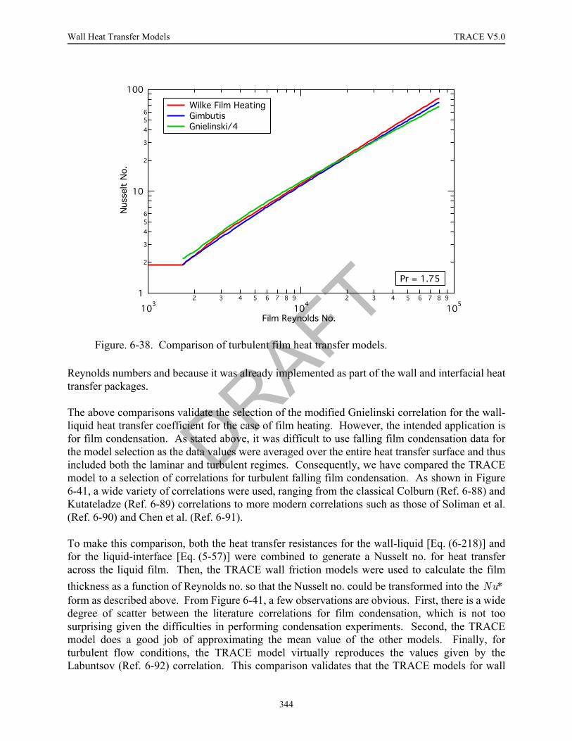
Wall Heat Transfer Models TRACE V5.0
Reynolds numbers and because it was already implemented as part of the wall and interfacial heattransfer packages.
The above comparisons validate the selection of the modified Gnielinski correlation for the wall-liquid heat transfer coefficient for the case of film heating. However, the intended application isfor film condensation. As stated above, it was difficult to use falling film condensation data forthe model selection as the data values were averaged over the entire heat transfer surface and thusincluded both the laminar and turbulent regimes. Consequently, we have compared the TRACEmodel to a selection of correlations for turbulent falling film condensation. As shown in Figure6-41, a wide variety of correlations were used, ranging from the classical Colburn (Ref. 6-88) andKutateladze (Ref. 6-89) correlations to more modern correlations such as those of Soliman et al.(Ref. 6-90) and Chen et al. (Ref. 6-91).
To make this comparison, both the heat transfer resistances for the wall-liquid [Eq. (6-218)] andfor the liquid-interface [Eq. (5-57)] were combined to generate a Nusselt no. for heat transferacross the liquid film. Then, the TRACE wall friction models were used to calculate the filmthickness as a function of Reynolds no. so that the Nusselt no. could be transformed into the form as described above. From Figure 6-41, a few observations are obvious. First, there is a widedegree of scatter between the literature correlations for film condensation, which is not toosurprising given the difficulties in performing condensation experiments. Second, the TRACEmodel does a good job of approximating the mean value of the other models. Finally, forturbulent flow conditions, the TRACE model virtually reproduces the values given by theLabuntsov (Ref. 6-92) correlation. This comparison validates that the TRACE models for wall
Figure. 6-38. Comparison of turbulent film heat transfer models.
Nu∗
DRAFT
344

TRACE V5.0 Wall Heat Transfer Models FOOBAR1234FOOBAR1234FOOBAR1234FOOBAR1234FOOBAR1234
Wall H
eat T
ransfer M
odels
Figure. 6-39. Comparison of candidate film heat transfer models with the falling film heating data of Bays (Ref. 6-86) for water.
Figure. 6-40. Comparison of candidate film heat transfer models with the falling film heating data of Gimbutis (Ref. 6-85), Wilke (Ref. 6-84), and Ueda (Ref. 6-87).
! "##$! % &
#' (# )
!"
# $ % "
& '"
# $ $ DRAFT
345

Wall Heat Transfer Models TRACE V5.0
drag, wall-liquid heat transfer, and interfacial heat transfer all work together correctly to provide agood estimate for film condensation heat transfer in turbulent flow.
Dropwise Condensation
There is no explicit dropwise condensation model in the TRACE code as dropwise condensationusually only occurs for non-wettable surfaces. During TRACE simulations, however, conditionscan arise where the heat transfer mode is condensation but there is not enough liquid present towet the surface. Such a condition occurs, for example, during a transient when condensation isjust beginning so that a film has not yet had time to form. Similarly, for a vertical heat transfersurface undergoing condensation, the top-most node is often only partially wetted for the samereason. For such conditions, where only a fraction of the surface is covered with a liquid film, acondensation model is needed for the fraction of the surface that is "dry".
For film condensation, as described above, heat transfer occurs in a two-step process1;condensation occurs at the film surface with heat being removed first by interfacial heat transferto the liquid and thence to the wall. However, if there is not enough liquid present for a film toform, then the condensation heat flux must be removed directly from the vapor. That is,
Figure. 6-41. Comparison of TRACE model with literature correlations for falling film condensation.
1. It is a two-step process for pure-steam conditions, but a three-step process for condensation with non-con-densable gases with the additional step being the mass transfer that occurs in the steam-gas mixture.
! "
# "$
%&' (
) * + , $
DRAFT
346

TRACE V5.0 Wall Heat Transfer Models FOOBAR1234FOOBAR1234FOOBAR1234FOOBAR1234FOOBAR1234
Wall H
eat T
ransfer M
odels
(6-219)
where the subscript "DW" is used to indicate dropwise condensation. As dropwise condensationonly occurs for either a short period of time or for a small fraction of a heat transfer surface, anaccurate model is not required for TRACE. Indeed, there is no such thing as an accurate modelfor dropwise condensation. Instead, a model is required that simply provides a heat transfercoefficient that is large enough to get condensation started but not so large as to causecomputational difficulties.
To realize this in TRACE, the wall-gas heat transfer coefficient is simply set equal to the maximalvalue used for a liquid film. Thus, for pure-steam condensation,
(6-220)
where is the value for the minimum liquid film thickness. The value for was taken to
be 10 , so that the resulting condensation heat transfer coefficient would have the right orderof magnitude for dropwise condensation. This approach provides a degree of continuity ascondensation progresses and the surface becomes covered with a liquid film. Note, however, thatthis approach is only appropriate for pure-steam condensation. When non-condensable gases arepresent, the additional heat transfer resistance associated with the mass transfer process must beadded. This will be described in the next section.
The fraction of the heat transfer surface that is covered by a liquid film is estimated from the voidfraction using the thin film approximation,
(6-221)
Then, for the fraction of the wall that is wetted, the wall-liquid heat transfer is used,
(6-222)
and for the non-wetted fraction,
(6-223)
Non-Condensible Gas Effects
As described by Collier and Thome (Ref. 6-93), the presence of even a small quantity of non-condensable gas in the condensing vapor has a profound influence on the overall heat transfer
q″DW q″wg hwg Tw Tg–( )·= =
hwgkl
δmin-----------=
δmin δmin
µm
fwet1 α–( ) Dh·
4 δmin·-----------------------------=
hwl fwet hwl·=
hwg 1 fwet–( ) hwg·=
DRAFT
347

Wall Heat Transfer Models TRACE V5.0
resistance during condensation. The non-condensable gas is carried with the vapor towards theinterface where it accumulates so that the partial pressure of the vapor at the interface decreasesthereby decreasing the driving potential for heat transfer across the liquid film. The processlimiting the heat transfer rate then becomes the mass transfer rate for the vapor diffusing throughthe gas-vapor mixture to the interface. Indeed, as shown in Figure 10.4 of Reference 6-93,reductions of more than 50% in the heat transfer can be caused by air mass fractions as low as0.5% for a stagnant air-steam mixture.
To improve the predictive capability of the TRACE code for the Passive Containment CoolingSystem (PCCS) of the proposed ESBWR design, a new model for condensation in the presence ofnon-condensable gases was developed. Later, this model was extended to also be applicable tocondensation on the walls of the drywell itself. This new model for film condensation in thepresence of non-condensable gases employs the mass transfer conductance approach as developedby Kuhn et al. (Ref. 5-7) and was described previously in Chapter 5, Special Model for FilmCondensation.
During film condensation, the wall heat transfer coefficient is calculated using the models forwall-to-liquid heat transfer for laminar and turbulent films given by Eq. (6-212) and Eq. (6-218).The non-condensable gas effect, that normally controls the condensation rate, is calculated usingthe mass transfer model described previously in Chapter 5 and serves to augment the interfacialheat transfer resistance between the liquid and the gas-vapor mixture. This description of thismodel will not be repeated here but a comparison of its predicted heat transfer coefficients withthose of the UCB-Kuhn (Ref. 5-7) condensation experiments is given below.
Kuhn et al. (Ref. 5-7) conducted condensation experiments for cocurrent downflow in a tube withthe same diameter as that proposed for the PCCS condenser of the ESBWR design. In addition tothe pure-steam tests used above for the laminar film condensation model, they conducted both air-steam and helium-steam tests. We compared the TRACE model to all of the air-steam andhelium-steam data in the experiments of Kuhn. In these comparisons, the "total" heat transfercoefficient is defined as
(6-224)
There were 72 air-steam tests giving a total of 571 data points, the TRACE model calculated theheat transfer coefficient for these with an average error of 7.7% and an RMS error of 16.1% (seeFigure 6-42). Similarly, there were 25 helium-steam tests giving a total of 192 data points, theTRACE model calculated the heat transfer coefficient for these with an average error of 0.9% andan RMS error of 16.3% (see Figure 6-43). These values are considered to be within the errorbands associated with this data.
This film condensation model was extended to also be applicable for the conditions of the drywellwalls in the ESBWR design. For large containment volumes, the correlations used for turbulentforced convection in the mass transfer model needed to be replaced by something moreappropriate. For this purpose, the correlation for turbulent free convection on a vertical plate
hcondq″w
Tw Tsv–( )---------------------------=
DRAFT
348

TRACE V5.0 Wall Heat Transfer Models FOOBAR1234FOOBAR1234FOOBAR1234FOOBAR1234FOOBAR1234
Wall H
eat T
ransfer M
odels
Figure. 6-42. Comparison of condensation heat transfer coefficients calculated using the TRACE model with the air-steam data of Kuhn et al. (Ref. 5-7).
Figure. 6-43. Comparison of condensation heat transfer coefficients calculated using the TRACE model with the helium-steam data of Kuhn et al. (Ref. 5-7).
!"# ##$#
%$& '
()
)
DRAFT
349

Wall Heat Transfer Models TRACE V5.0
given by McAdams (Ref. 5-29) was chosen as detailed in Chapter 5, Special Model for FilmCondensation. Again, this model description will not be repeated here.
For the case of "dropwise" condensation, that is, when not enough liquid is present to cover thesurface with a film, the non-condensable gas effect must be applied directly to the wall-gas heattransfer coefficient. To accomplish this, the mass transfer and gas-side interfacial heat transfermodels described previously are used to compute the condensation and sensible heat fluxes thatwould occur if the liquid-side heat transfer resistance was negligible. Simply put, the iterative
procedure for the liquid-gas interface temperature is bypassed so that . Then, the wall-gas heat flux is computed from
(6-225)
and the heat transfer coefficient becomes
(6-226)
A comparison of this model was made to both the Uchida correlation (Ref. 5-30) and the Dehbidata (Ref. 5-31) with excellent results. Figure 6-44 presents this comparison to the Uchidacorrelation over a wide range of non-condensable gas mass fraction for atmospheric pressureconditions.
Figure. 6-44. Comparison of the TRACE model for wall condensation in the presence of non-condensable gases with the Uchida correlation at atmospheric pressure.
Ti Tw≈
q″wg q″cond q″sens+=
hwgq″cond q″sens+( )
Tw Tg–( )-----------------------------------------=
! "
#$
%&' ! DRAFT
350
TRACE V5.0 Wall Heat Transfer Models FOOBAR1234FOOBAR1234FOOBAR1234FOOBAR1234FOOBAR1234
Wall H
eat T
ransfer M
odels
This completes the description of the TRACE wall heat transfer models.
References6-1 M.S. Bhatti and R.K. Shah, "Turbulent and Transition Flow Convective Heat Transfer in
Ducts," Handbook of Single-Phase Convective Heat Transfer, eds. S. Kakac, R.K. Shah,and W. Aung, Chapter 4, Wiley-Interscience, New York, 1987.
6-2 F.P. Incropera and D.P. De Witt, Introduction to Heat Transfer, 2nd edition, Chapter 8,John Wiley & Sons, New York, 1990.
6-3 V. Gnielinski, "New Equations flow regime Heat and Mass Transfer in Turbulent Pipe andChannel Flow," Int. Chem. Eng., 16, 359-368, 1976.
6-4 G.K. Filonenko, "Hydraulic Resistance in Pipes," (in Russian), Teplonergetika, 1, 40-44,1954.
6-5 F. Kreith and M.S. Bohn, Principles of Heat Transfer, 4th edition, Chapter 6, page 289-290, Harper-Collins Publishers, New York, 1986.
6-6 W. Huschmidt and E. Burck, "The Effect of Temperature-Dependent Properties ofMaterials on Heat Transfer in the Turbulent Flow of Liquids in Tubes at High Heat Fluxesand Prandtl Numbers," Int. J. Heat Mass Transfer, 11, 1041-1048, 1968.
6-7 J.P Holman, Heat Transfer, 5th edition, Table 7.1, McGraw-Hill Book Co., Inc., NewYork, 1981.
6-8 J. Weisman, "Heat Transfer to Water Flowing Parallel to Tube Bundles," Nuclear Scienceand Engineering, 6, 78-79, 1959.
6-9 A. Ya. Inayatov, "Correlation of Data on Heat Transfer. Flow Parallel to Tube Bundles atRelative Tube Pitches of 1.1 < s/d < 1.6," Heat Transfer - Soviet Research, 7, 84-88, 1975.
6-10 M.S. El-Genk, B. Su, and Z. Guo, "Experimental Studies of Forced, Combined andNatural Convection of Water in Vertical Nine-Rod Bundles with a Square Lattice," Int. J.Heat Mass Transfer, 36, 2359-2374, 1993.
6-11 J.H. Kim and W.-H. Li, "Heat Transfer in Laminar Flow Along Circular Rods in InfiniteSquare Arrays," J. Heat Transfer, 110, 252-257, 1988.
6-12 P.K. Sarma, C.V.N. Sastry, and V.N. Murthy, "Experimental Investigation of CombinedForced and Free Convective Heat Transfer Rates in a Vertical U-Tube with One LegHeated," Proceedings of the 7th International Heat Transfer Conference, Vol. 3, 471-476,1982.
DRAFT
351

Wall Heat Transfer Models TRACE V5.0
6-13 J. C. Chen, "A Correlation for Boiling Heat Transfer to Saturated Fluids in ConvectiveFlow," presented to 6th National Heat Transfer Conference, Boston, 11-14 Aug., ASMEpreprint 63-HT-34, 1963.
6-14 D. Kim et al, "Comparison of 20 Two-Phase Heat Transfer Correlations with Seven Setsof Experimental Data, Including Flow Pattern and Tube Inclination Effects," HeatTransfer Engineering, 20, 15-40, 1999.
6-15 M.A. Aggour, M.M. Vijay, and G.E. Sims, "A Correlation of Mean Heat TransferCoefficients for Two-Phase Two-Component Flow in a Vertical Tube," Proceedings of the7th International Heat Transfer Conference, Vol. 5, 367-372, 1982.
6-16 K.S. Rezkallah and G.E. Sims, "An Examination of Correlations of Mean Heat TransferCoefficients in Two-Phase Two-Component Flow in Vertical Tubes," AIChE SymposiumSeries, 83 (257), 109-114, 1987.
6-17 J.G. Collier, Convective Boiling and Condensation, p. 382-406, McGraw-Hill, London,1972.
6-18 N. Basu, G.R. Warrier, and V.K. Dhir, "Onset of Nucleate Boiling and Active NucleationSite Density During Subcooled Flow Boiling," J. Heat Transfer, 124, 717-728, 2002.
6-19 A. E. Bergles and W. M. Rohsenow, "The Determination of Forced Convection SurfaceBoiling Heat Transfer," J. Heat Transfer, 86, 365-372, 1964.
6-20 E. J. Davis and G. H. Anderson, "The Incipience of Nucleate Boiling in ForcedConvection Flow," AIChE Journal, 12(4), 774-780, 1966
6-21 J.C. Chen, "A Correlation for Boiling Heat Transfer to Saturated Fluids in ConvectiveFlow," ASME preprint 63-HT-34 presented at 6th National Heat Transfer Conference,Boston, 11-14 August, 1963.
6-22 M. G. Cooper, "Heat Flow Rates in Saturated Nucleate Boiling - a Wide-RangingExamination Using Reduced Properties," Adv. Heat Transfer, 16, 157-239, 1984.
6-23 D. Gorenflo, "Pool Boiling," VDI-Heat Atlas, Sect. Ha, VDI-Verlag, Dusseldorf, 1993.Obtained from secondary reference: J.G. Collier and J. R. Thome, Convective Boiling andCondensation, 3rd Edition, p. 155-158, Oxford University Press, Oxford, 1994.
6-24 W. H. Jens and P. A. Lottes, "Analysis of Heat Transfer Burnout, Pressure Drop andDensity Data for High Pressure Water," ANL-4627, May 1951.
6-25 S. Levy, "Generalized Correlation of Boiling Heat Transfer," J. Heat Transfer, 81C, 37-42, 1959.
DRAFT
352

TRACE V5.0 Wall Heat Transfer Models FOOBAR1234FOOBAR1234FOOBAR1234FOOBAR1234FOOBAR1234
Wall H
eat T
ransfer M
odels
6-26 W. H. McAdams, et al., "Heat Transfer at High Rates to Water with Surface Boiling," Ind.Eng. Chem., 41, 1945-1955, 1949.
6-27 D. Steiner and J. Taborek, "Flow Boiling Heat Transfer in Vertical Tubes Correlated by anAsymptotic Model," Heat Transfer Engng., 13(2), 43-69, 1992.
6-28 J. R. S. Thom, et al., "Boiling in Subcooled Water During Flow Up Heated Tubes orAnnuli," Paper 6 presented at the Symposium on Boiling Heat Transfer in SteamGeneration Units and Heat Exchangers held in Manchester, IMechE (London) 15-16September, 1965.
6-29 W.H. McAdams, Heat Transmission, 3rd Edition, p. 378, McGraw-Hill, New York, 1954.
6-30 S. S. Kutateladze, "Boiling Heat Transfer," Int. J. Heat Mass Transfer, 4, 3-45, 1961
6-31 S. W. Churchill, The Interpretation and Use of Rate Data, Hemisphere, New York, 1974.
6-32 J. P. Holman, Heat Transfer, 8th Edition, McGraw-Hill, New York, p. 536, 1997.
6-33 R. W. Bjorge, G. R. Hall and W. M. Rohsenow, "Correlation of Forced Convection BoilingHeat Transfer Data," Int. J. Heat Mass Transfer, 25(6), 753-757, 1982.
6-34 R. T. Lahey, Jr., "A Mechanistic Subcooled Boiling Model," Heat Transfer 1978,Proceedings of the 6th International Heat Transfer Conference, Toronto, Canada, Vol. 1,293-297, 1978.
6-35 P. Saha and N. Zuber, "Point of Net Vapor Generation and Vapor Void Fraction inSubcooled Boiling," Heat Transfer 1974, Proceedings of the 5th International HeatTransfer Conference, Tokyo, Japan, Vol. 4, 175-179, 1974.
6-36 D. C. Groeneveld, et al., "The 1995 Look-Up Table for Critical heat Flux in Tubes," Nucl.Eng. Des., 163, 1-23, 1996.
6-37 D. C. Groeneveld, S. C. Cheng and T. Doan, "1986 AECL-UO Critical Heat Flux LookupTable," Heat Trans. Eng., 7, 46-62, 1986.
6-38 D. C. Groeneveld, et al., "A General Method of Predicting Critical Heat Flux in AdvancedWater-Cooled Reactors," Proceedings of the 9th International Topical Meeting on NuclearReactor Thermal Hydraulics (NURETH-9), San Francisco, California, October 1999.
6-39 N. Zuber, "Hydrodynamic Aspects of Boiling Heat Transfer," AECU-4439, AtomicEnergy Commission, 1959
6-40 H. J. Ivey and D. J. Morris, "On the Relevance of the Vapour-Liquid ExchangeMechanism for Subcooled Boiling Heat Transfer at High Pressure," AEEW-R-137, UnitedKingdom Atomic Energy Authority Research Group, 1962.
DRAFT
353

Wall Heat Transfer Models TRACE V5.0
6-41 P. Griffith, C. T. Avedisian and J. P. Walkush, "Counterflow Critical Heat Flux," AIChESymposium Series, No. 174, Vol. 74, 149-155, 1978.
6-42 L. Biasi et al., "Studies in Burnout, Part 3: A New Correlation for Round Ducts andUniform Heating and Its Comparison with World Data," Energ. Nucl., 14, 530-536, 1967.
6-43 S. Bertoletti et al., "Heat Transfer Crisis with Steam-Water Mixtures," Energ. Nucl., 12(3),1965.
6-44 J. A. Borkowski and N. L. Wade, editors, "TRAC-BF1/MOD1 Models and Correlations,"NUREG/CR-4391, Section 4.2.12, 1992.
6-45 R. E. Phillips, R. W. Shumway and K. H. Chu, "Improvements to the Prediction of BoilingTransition in BWR Transient Calculations," Proceedings of the 20th ASME/AIChENational Heat Transfer Conference, Milwaukee, WI, August 1981.
6-46 P. J. Berenson, "Film Boiling Heat Transfer from a Horizontal Surface," J. Heat Transfer,p. 351-358, August 1961.
6-47 M. J. Thurgood et al., "COBRA/TRAC - A Thermal-Hydraulics Code for TransientAnalysis of Nuclear Reactor Vessels and Primary Coolant Systems," Vol. 1, NUREG/CR-3046, 1983.
6-48 D. Swinnerton, K. G. Pearson, and M. L. Hood, "Steady State Post Dryout Experiments atLow Quality and Medium Pressure," United Kingdom Atomic Energy Authority, AEEW-R 2192, 1988.
6-49 J. C. Stewart and D. C. Groeneveld, "Low-Quality and Subcooled Film Boiling of Waterat Elevated Pressures," Nucl. Eng. Des., 67, 259-272, 1981.
6-50 V. K. Dhir and G. P. Purohit, "Subcooled Film Boiling Heat Transfer from Spheres," Nucl.Eng. Des., 47, 49-66, 1978.
6-51 Y. Koizumi, et al., "High-Pressure Reflooding Experiments of Multi-Rod Bundle atROSA-IV TPTF," Nucl. Eng. Design, 120, 301-310, 1990.
6-52 G. Xu, H. Kumamaru, and K. Tasaka, "Reflood Experiments in Single Rod Channel UnderHigh-Pressure Condition," Japan Atomic Energy Research Institute, JAERI-M 89-178,1989.
6-53 M. J. Loftus et al., "PWR FLECHT-SEASET Unblocked Bundle, Forced and GravityReflood Task Data Report," NUREG/CR-1532, 1981.
6-54 T. M. Anklam, "ORNL Small-Break LOCA Heat Transfer Test Series I: High-PressureReflood Analysis," NUREG/CR-2114, 1981.
DRAFT
354

TRACE V5.0 Wall Heat Transfer Models FOOBAR1234FOOBAR1234FOOBAR1234FOOBAR1234FOOBAR1234
Wall H
eat T
ransfer M
odels
6-55 C. R. Hyman, T. M. Anklam and M. D. White "Experimental Investigations of BundleBoiloff and Reflood Under High-Pressure Low Heat Flux Conditions," NUREG/CR-2455, 1982.
6-56 V. K. Dhir, R. B. Duffey, and I. Catton, "Quenching Studies on a Zircaloy Rod Bundle," J.Heat Transfer, 103, 293-299, 1981.
6-57 "RELAP5/Mod3.3 Code Manual, Volume IV: Models and Correlations," NUREG/CR-5535, Rev. 1, Vol. IV, 2001.
6-58 D. R. Liles et al., "TRAC-PF1/MOD1: Correlations and Models," NUREG/CR-5069,1988.
6-59 W. L. Kirchner, "Reflood Heat Transfer in a Light Water Reactor," Ph.D Thesis,Massachusetts Institute of Technology, NUREG-0106, 1976.
6-60 T. A. Bjornard and P. Griffith, "PWR Blowdown Heat Transfer," Thermal and HydraulicAspects of Nuclear Reactor Safety, American Society of Mechanical Engineers, NewYork, Vol. 1, 17-41, 1977.
6-61 K. Johannsen, P. Weber, and Q. Feng, "Experimental Investigation of Heat Transfer in theTransition Region," Commission of the European Communities, EUR 13235 EN, 1990.
6-62 K. K. Fung, "Subcooled and Low Quality Film Boiling of Water in Vertical Flow atAtmospheric Pressure," NUREG/CR-2461, 1981.
6-63 F. de Cachard, "Development, Implementation, and Assessment of Specific Closure Lawsfor Inverted-Annular Film-Boiling in a Two-Fluid Model," NUREG/IA-0133, 1996.
6-64 N. Hammouda, D. C. Groeneveld and S. C. Cheng, "Two-Fluid Modeling of InvertedAnnular Film Boiling," Int. J. Heat Mass Transfer, 40(11), 2655-2670, 1997.
6-65 R. P. Forslund and W. M Rohsenow, "Dispersed Flow Film Boiling," J. Heat Transfer,90(6), 399-407, 1968.
6-66 C. A. Sleicher and M. W. Rouse, "A Convenient Correlation for Heat Transfer to Constantand Variable Property Fluids in Turbulent Pipe Flow," Int. J. Heat Mass Transfer, 18, 677-683, 1975.
6-67 B. S. Petukhov, "Turbulent Heat Transfer in Tubes with Variable Fluid Properties,"Chapter 9, Heat Exchanger Sourcebook, edited by J. W. Palen, Hemisphere, Washington,1986.
6-68 M. Molki and E. M. Sparrow, "An Empirical Correlation for the Average Heat TransferCoefficient in Circular Tubes," J. Heat Transfer, 108, 482-484, 1986.
DRAFT
355
Wall Heat Transfer Models TRACE V5.0
6-69 A. F. Mills, "Experimental Investigation of Turbulent Heat Transfer in the EntranceRegion of a Circular Conduit," J. Mech. Eng. Sci., 4, 63-77, 1962.
6-70 P. M. Worsoe-Schmidt and G. Leppert, "Heat Transfer and Friction for Laminar Flow of aGas in a Circular Tube at High Heating Rate," Int. J. Heat Mass Transfer, 8, 1281-1301,1965.
6-71 W.H. McAdams, Heat Transmission, 3rd Edition, Chapter 7, Eq. (7-4a), McGraw-HillBook Co., New York, NY, 1954.
6-72 B. Metais and E. R. G. Eckert, "Forced, Mixed, and Free Convection Regimes," J. HeatTransfer, 295-296, May 1964.
6-73 S. M. Nijhawan, "Experimental Investigation of Thermal Non-Equilibrium in Post-DryoutSteam-Water Flow," Ph.D Thesis, Lehigh University, 1980.
6-74 D. G. Evans, S. W. Webb, and J. C. Chen, "Measurement of Axially VaryingNonequilibrium in Post-Critical-Heat-Flux Boiling in a Vertical Tube," NUREG/CR-3363, Vol. 2, 1983.
6-75 D. P. Frankum, J. C. Ralph, and C. D. Wade, "Post Dryout Heat Transfer and Void FractionMeasurements at Low Flow and 2-4 Bar Pressure," United Kingdom Atomic EnergyAuthority, Harwell, PWR/HTWG/P(90)777 and G-5415, 1990.
6-76 R. A. Savage, D. Swinnerton, and K. G. Pearson, "Steady State Post Dryout Experimentsat Low Quality and Medium Pressure," United Kingdom Atomic Energy Authority,AEEW-R 2486, 1989.
6-77 A. N. Bhaskarwar and M. S. Phanikumar, "On Heat Transfer Augmentation Using DiluteGas-Solid Suspensions," J. Heat Transfer, 117, 1091-1094, 1995.
6-78 S. W. Webb and J. C. Chen, "A Two-Region Vapor Generation Rate Model for ConvectiveFilm Boiling," Proceedings of the 1st International Workshop on Fundamental Aspects ofPost-Dryout Heat Transfer, Salt Lake City, NUREG/CP-0060, p 485-508, 1984.
6-79 A. J. Clare and S. A. Fairbairn, "Droplet Dynamics and Heat Transfer in Dispersed Two-Phase Flow," Proceedings of the 1st International Workshop on Fundamental Aspects ofPost-Dryout Heat Transfer, Salt Lake City, NUREG/CP-0060, p 373-396, 1984.
6-80 M. I. Drucker, V. K. Dhir, and R. B. Duffey, "Two-Phase Heat Transfer for Flow in Tubesand Over Rod Bundles with Blockages," J. Heat Transfer, 106, 856-864, 1984.
6-81 H. Kianjah, V. K. Dhir, and A. Singh, "An Experimental Study of Heat TransferEnhancement in Disperse Flow in Rod Bundles," Proceedings of the 1st InternationalWorkshop on Fundamental Aspects of Post-Dryout Heat Transfer, Salt Lake City,NUREG/CP-0060, p 397-415, 1984.
DRAFT
356

TRACE V5.0 Wall Heat Transfer Models FOOBAR1234FOOBAR1234FOOBAR1234FOOBAR1234FOOBAR1234
Wall H
eat T
ransfer M
odels
6-82 K. H. Sun, J. M. Gonzalez-Santalo, and C. L. Tien, "Calculations of Combined Radiationand Convection Heat Transfer in Rod Bundles Under Emergency Cooling Conditions," J.Heat Transfer, 414-420, August 1976.
6-83 S. Z. Kuhn, P. F. Peterson, and V. E. Schrock, "Interfacial Shear and Waviness Effects onLaminar Film Flow Heat Transfer in Vertical Tubes," Proceedings of the 31st NationalHeat Transfer Conference, Houston, 4, 79-89, 1996.
6-84 W. Wilke, "Heat Transfer in Rippling Films," Ver. Deut. Ingr. Forshungsh., 490, 1962.
6-85 G. J. Gimbutis, "Heat Transfer of a Turbulent Vertically Falling Film," Heat Transfer 1974,Proceedings of the 5th International Heat Transfer Conference, Tokyo, Vol. 2, 85-89, 1974.
6-86 G. S. Bays and W. H. McAdams, "Heat Transfer Coefficients in Falling Film Heaters:Streamline Flow," Ind. Eng. and Chem., 29 (11), 1240-1246, 1937.
6-87 T. Ueda, et al., "Heat Transfer and Pressure Drop for Flow Condensation Inside a VerticalTube," Bulletin of the JSME, 15, No. 88, 1267-1277, 1972.
6-88 A. P. Colburn, "The Calculation of Condensation Where a Portion of the CondensateLayer is in Turbulent Flow," Trans. AIChE, 30, 187-193, 1933.
6-89 S. S. Kutateladze, Fundamentals of Heat Transfer, p. 307, Academic Press, New York,1963.
6-90 M. Soliman, J. R. Schuster, and P. J. Berenson, "A General Heat Transfer Correlation forAnnular Flow Condensation," J. Heat Transfer, 90, 267-276, 1968.
6-91 S. L. Chen, F. M. Gerner, and C. L. Tien, "General Film Condensation Correlations,"Experimental Heat Tranfer, 1, 93-107, 1987.
6-92 D. A. Labuntsov, "Condensation of Steam on a Vertical Surface with TurbulentCondensate Film," Inzh. Fiz. Zhur,, 3(8), 3-8, 1960.
6-93 J.G. Collier and J. R. Thome, Convective Boiling and Condensation, 3rd Edition, p. 439-445, Oxford University Press, Oxford, 1994.
6-94 R. Shumway, "Consolidation of TRAC Codes: Task CHAN," Scientech Internal ReportSCIE-NRC-375-99, NRC ADAMS Accession No. ML071710042, (January 12, 1999).
DRAFT
357

Wall Heat Transfer Models TRACE V5.0
DRAFT
358

TRACE V5.0 Flow Process Models FOOBAR1234FOOBAR1234FOOBAR1234FOOBAR1234FOOBAR1234FOOBAR1234
Flow Process
Models
7 Flow Process Models
FOOBAR1234FOOBAR1234FOOBAR1234FOOBAR1234FOOBAR1234FOOBAR1234FOOBAR1234
Special models play an important role in the overall performance of TRACE. In the followingsections, four special models are described:
•models for critical flow,
• countercurrent flow,
•offtake flow from a large pipe in horizontal stratified flow,
• form loss, and
NomenclatureThe nomenclature that applies to this section follows:
= homogeneous equilibrium sound speed
= flow area
= flow area before the abrupt expansion
= flow area after the abrupt expansion
= virtual mass coefficient
= abscissa intercept in Bankoff CCFL correlation
= interfacial drag coefficient
, = correlation constants in offtake model
= diameter
= interpolation constant used in the CCFL model
= gravitational acceleration constant
= characteristic height from liquid surface to offtake entrance plane
aHE
A
Aj
Aj 1+
C
CB
Ci
C1 C2
D
E
g
h
DRAFT
359

Flow Process Models TRACE V5.0
= critical entrainment height
= latent heat of vaporization
= dimensionless gas flux
= dimensionless liquid delivery
= superficial velocity
= critical wave number
= additive loss factor or kinetic energy (in level tracking model)
= length or water level height (in level tracking model)
= Bond number
= slope in the Bankoff CCFL correlation
= number of holes in the tie plate
= pressure
= pressure at the choking plane
= pressure upstream of the choking plane
= heat flux from the saturation interface to the liquid field
= heat flux from the saturation interface to the gas field
= flux of direct sensible heat to the liquid field
= flux of direct sensible heat to the gas field
= gas constant or nondimensional height ratio for offtake model
= entropy
= time
= thickness of the tie plate
= temperature
= stagnation temperature
= velocity
= critical velocity for single-phase vapor
= subcooled-liquid choking velocity
= velocity upstream of the choking plane
hb
hfg
Hg
Hl
j
kc
K
L
L∗
MB
n
P
Pc
Pup
qil
qig
qdl
qdg
R
s
t
tp
T
To
V
Vcg
Vcl
Vup
DRAFT
360

TRACE V5.0 Flow Process Models FOOBAR1234FOOBAR1234FOOBAR1234FOOBAR1234FOOBAR1234FOOBAR1234
Flow Process
Models
= volume
= mass flow rate in offtake model
= distance or offtake flow quality
Greek = gas volume fraction
= specific heat ratio or mass, energy and volume flux time weighting factor
= temperature difference
= time step size
= cell height
= interfacial mass exchange term
= characteristic roots
= distance between liquid-gas interface and cell boundaries
= density
= difference between the phasic densities
= mass flux
= energy flux
= potential energy
= surface tension
= ratio of the area of the holes in the tie plate to the total area of the tie plate
= volume flux
Subscripts = noncondensable gas
= cell-centered value
= a cutoff value
= edge variables
= combined-gas mixture
= denotes a cell index location (could also be , , , etc)
= phase index (liquid or gas)
= applies to the water level
Vol
W
x
α
γ
T∆
t∆
x∆
Γi
λi
λE
ρ
ρ∆
φ
ζ
Φ
σ
η
ω
a
c
cut
E
g
j j 1+ j 1 2⁄+ j 1 2⁄–
k
L
DRAFT
361

Flow Process Models TRACE V5.0
= liquid
= denotes the cell that contains the water level
= total mixture
= conditions upstream of the choking plane
= vapor
= edge-based value (may be accompanied by a + or - superscript to indicate which side of cell center the edge is on)
Superscripts = applies to the water level
= current-time quantity
= new-time quantity
= predicted quantity
= above the water level
= below the water level
Critical FlowCritical (or "choked") flow occurs when the mass flow in a pipe becomes independent of thedownstream conditions. Therefore, a further reduction in the downstream pressure will notchange the mass flow rate. The reason choking occurs is that acoustic signals can no longerpropagate upstream to affect the boundary conditions that determine the mass flow rate at thechoke plane. There are numerous examples in the operation of a nuclear power plant where thepresence of critical flow can play a large role in how the plant responds during some hypotheticaltransient. Predicting such phenomena during reactor safety simulations can therefore be key toachieving an accurate overall understanding of the scenario being simulated.
Because the TRACE fluid-dynamics equations for one-dimensional components use a multi-stepprocedure that allows the material Courant condition to be violated, the presence of critical flowcan be predicted for components with smooth area changes simply by using a sufficiently finenodalization. The computational efficiency of models that employ this technique, however,generally makes this approach cost prohibitive. For 1-D components with abrupt area changes,this technique can also be problematic as a fine nodalization can cause erroneous natural chokingresults. As a result, a separate choking model that will allow TRACE to predict critical flow isalmost a necessity (Ref. 7-1).
The basic thrust of the critical flow model is to predict, for a given cell edge, the conditions forwhich choked flow would be expected to occur. Then, by comparing the momentum solution
l
lev
m
up
v
e
L
n
n 1+
p
+
-
DRAFT
362
TRACE V5.0 Flow Process Models FOOBAR1234FOOBAR1234FOOBAR1234FOOBAR1234FOOBAR1234FOOBAR1234
Flow Process
Models
predictions against these conditions, TRACE can determine whether the flow is actually chokedat a particular cell edge, and adjust the velocity and associated pressure derivatives accordingly.Because the predictions of the choking criteria are highly dependent upon the nature of the flowfield at the cell-edge and upstream cell-center, the critical flow model is really three separatemodels in one:
• a subcooled-liquid choked-flow model
• a two-phase, two-component choked-flow model
• a single-phase vapor choked-flow model
Each of these models will be addressed separately in the sub-sections that follow.
The critical flow model in TRACE is implemented as a modeling option that you may turn on oroff at individual cell edges in each 1D component. Each edge location may also have associatedwith it, one of four pairs of user-defined subcooled and two-phase choked-flow multipliers.Depending on which choking model is used (either subcooled-liquid, two-phase two-componentfluid, or superheated vapor), these multipliers allow you to adjust the predicted liquid, steam/gas-mixture, or both, choking velocities to account for break or nozzle geometry effects. The use ofthese multipliers is described more completely in the TRACE User’s Guide.
Subcooled Liquid
The subcooled choked-flow model is a modified form of the Burnell model (Ref. 7-2) and isessentially the same as that used in RELAP5 (Ref. 7-3). The physical process that occurs duringthe subcooled blowdown phase is described in the following paragraphs. Much of the discussionpresented here has simply been repeated directly from Reference 7-3.
Initially, and in the early phase of blowdown , the flow approaching the break or break nozzle willbe subcooled liquid. Under most conditions of interest in LWR systems, the fluid changes phaseat the break because the downstream pressure is much lower than the saturation pressurecorresponding to the system fluid temperature. The transition from single- to two-phase flow,which is accompanied by a nearly discontinuous change in the fluid bulk modulus (measure of itscompressibility), leads to a large discontinuity in the sound speed at the break. This is especiallytrue for the liquid to liquid-vapor transition (for example, at 600 kPa, the ratio of single- to two-phase sound speed at the liquid boundary is 339.4. An effective discontinuity is also present atthe vapor boundary, but the ratio is only 1.069). Thus considerable care must be exercised whenanalyzing a flow having transitions to or from a pure phase.
To understand the physical process that occurs for subcooled upstream conditions, consider theflow through a converging/diverging nozzle connected to an upstream plenum with subcooledwater at a high pressure. For a downstream pressure only slightly lower than the upstreampressure, subcooled liquid flow will exist throughout the nozzle. Under these conditions, the flowcan be analyzed using Bernoulli’s equation, which predicts a minimum pressure, , at the
throat1. As the downstream pressure is lowered further, a point is reached where the throat
Pt
DRAFT
363

Flow Process Models TRACE V5.0
pressure equals the local saturation pressure, . If the downstream pressure is lowered further,
vaporization will take place at the throat1. When this happens, the fluid sound speed lowersdrastically; but continuity considerations dictate that the velocity, , of the two-phase mixture (atthe point of minuscule void fraction) just equals the velocity of the subcooled water slightlyupstream of the throat. When this occurs, in the subcooled region is less than the water soundspeed, ; but in the two-phase region, can be greater than the two-phase sound speed, .
Hence, the subcooled water has a Mach number ( ) < 1, whereas the two-phase mixture at thethroat has . Under these conditions ( in the two-phase region), downstreampressure effects cannot be propagated upstream, so the flow is considered to be choked. Inparticular, the supersonic two-phase fluid at the throat must increase in velocity and the pressuremust drop as it expands in the diverging section2. We should be careful to note, however, thattransition back to subsonic flow can occur in the nozzle as a result of a shock wave. This chokedcondition is shown in Figure 7-1, along with the corresponding sound speed and velocity profiles.Contrary to the usual single-phase choked flow in a converging/diverging nozzle, there is no pointin the flow field where . This is because in the homogeneous equilibrium model the fluidundergoes a discontinuous change in sound speed from single-phase subcooled conditions to two-phase conditions, although the fluid properties are continuous through the transition point.
The liquid velocity at the throat can be calculated from Bernoulli’s equation, assuming steady,frictionless, incompressible flow, such that
, (7-1)
where the subscript refers to values at the throat and the subscript refers to the upstreamvalues. The throat pressure, , is equal to the nucleation pressure, , and can be considerably
lower than the local saturation pressure, , because thermal nonequilibrium effects can causenucleation delay.
Any further reduction in the downstream pressure does not affect the flow because thedisturbance cannot move upstream where the flow is supersonic in the diverging section. Thus,Eq. (7-1) gives the liquid throat velocity for any downstream pressure lower than the pressurenecessary to cause the subcooled liquid to begin flashing at the throat (which is the case for mostproblems of interest in LWR applications).
1. For all practical cases of choking, the subcooled water can be considered incompressible with infinite sound speed.
1. An idealized one-dimensional homogeneous equilibrium model is assumed.2. In a supersonic flow, a diverging nozzle implies an increase in velocity.
Psat
vt
vtaliq vt aHE
MM 1> M 1>
M 1=
Vt Vup2 2 pup pt–( )
ρl---------------------------+
12---
=
t uppt pnuc
psatDRAFT
364
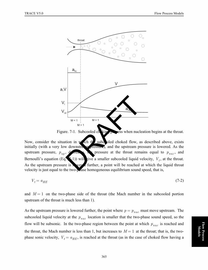
TRACE V5.0 Flow Process Models FOOBAR1234FOOBAR1234FOOBAR1234FOOBAR1234FOOBAR1234FOOBAR1234
Flow Process
Models
Now, consider the situation in which the subcooled choked flow, as described above, existsinitially (with a very low downstream pressure), and the upstream pressure is lowered. As theupstream pressure, , decreases, the pressure at the throat remains equal to , and
Bernoulli’s equation (Eq. (7-1)) will give a smaller subcooled liquid velocity, , at the throat.As the upstream pressure is lowered further, a point will be reached at which the liquid throatvelocity is just equal to the two-phase homogeneous equilibrium sound speed, that is,
(7-2)
and on the two-phase side of the throat (the Mach number in the subcooled portionupstream of the throat is much less than 1).
As the upstream pressure is lowered further, the point where must move upstream. Thesubcooled liquid velocity at the location is smaller that the two-phase sound speed, so the
flow will be subsonic. In the two-phase region between the point at which is reached and
the throat, the Mach number is less than 1, but increases to at the throat; that is, the two-phase sonic velocity, , is reached at the throat (as in the case of choked flow having a
Figure. 7-1. Subcooled choking process when nucleation begins at the throat.
M < 1 M > 1
aHE
V
a,V
M > 1
throat
aliq
Vt
Vup
pup pnuc
Vt
Vt aHE=
M 1=
p pnuc=pnuc
pnuc
M 1=Vt aHE=
DRAFT
365

Flow Process Models TRACE V5.0
continuous variation of sound speed with pressure). As the upstream pressure is reduced evenfurther, the point moves upstream until complete two-phase flow exists. Therefore, themaximum of the Burnell expression and the homogeneous equilibrium sound speed give thesubcooled choking criterion. Thus,
. (7-3)
In TRACE, a nucleation delay model, developed by Alamgir and Leinhard (Ref. 7-4) andimproved upon by Jones (Ref. 7-5) and Abuaf (Ref. 7-6), determines the cell-edge pressure, ,
from the saturation pressure, (corresponding to the upstream liquid temperature, ), suchthat
(7-4)
where is the surface tension, is the upstream liquid temperature, is the critical
temperature, is the substantial derivative of the pressure, is the Boltzmann constant,
and are cell-edge phasic densities, is the throat (cell-edge) velocity, and and arethroat and upstream (nozzle inlet) flow areas.
Equations (7-3) and (7-4) form a set of coupled equations that, through iteration, can be solved todetermine the throat velocity that will result when the flow is choked. By comparing the velocity,as calculated by the momentum solution, against this predicted choke velocity, TRACE is able todetermine whether, in fact, choked flow has occurred and thereby take the necessary steps toaccount for this in the time solution procedure. The calculational sequence for the TRACEsubcooled-liquid choking model is described in Appendix C.
pnuc
Vt Max aHE Vup2 2 pup pt–( )
ρl---------------------------+
12---
,
⎩ ⎭⎪ ⎪⎨ ⎬⎪ ⎪⎧ ⎫
=
pt
psat Tl
pt pnuc psat Max 0.0 0.258
σ1.5 TlTc------
⎝ ⎠⎜ ⎟⎛ ⎞
13.76
1 13.25 1
1.01325 11×10---------------------------------– Dp
Dt-------
⎝ ⎠⎜ ⎟⎛ ⎞
0.8
+
kTc( )0.5 1ρgρl-----–⎝ ⎠
⎛ ⎞---------------------------------------------------------------------------------------------------------------------------,–= =
27 0.072( )2AtAup---------
⎝ ⎠⎜ ⎟⎛ ⎞
2 ρlVt2
2-----------–
σ Tl Tc
Dp Dt⁄ k ρl
ρg Vt At Aup
DRAFT
366
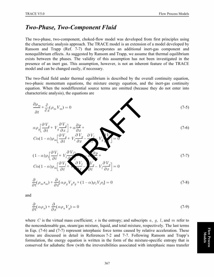
TRACE V5.0 Flow Process Models FOOBAR1234FOOBAR1234FOOBAR1234FOOBAR1234FOOBAR1234FOOBAR1234
Flow Process
Models
Two-Phase, Two-Component Fluid
The two-phase, two-component, choked-flow model was developed from first principles usingthe characteristic analysis approach. The TRACE model is an extension of a model developed byRansom and Trapp (Ref. 7-7) that incorporates an additional inert-gas component andnonequilibrium effects. As suggested by Ransom and Trapp, we assume that thermal equilibriumexists between the phases. The validity of this assumption has not been investigated in thepresence of an inert gas. This assumption, however, is not an inherent feature of the TRACEmodel and can be changed easily, if necessary.
The two-fluid field under thermal equilibrium is described by the overall continuity equation,two-phasic momentum equations, the mixture energy equation, and the inert-gas continuityequation. When the nondifferential source terms are omitted (because they do not enter intocharacteristic analysis), the equations are
(7-5)
(7-6)
(7-7)
(7-8)
and
(7-9)
where is the virtual mass coefficient; is the entropy; and subscripts , , , and refer tothe noncondensable gas, steam/gas mixture, liquid, and total mixture, respectively. The last termsin Eqs. (7-6) and (7-7) represent interphasic force terms caused by relative acceleration. Theseterms are discussed in detail in References 7-2 and 7-7. Following Ransom and Trapp’sformulation, the energy equation is written in the form of the mixture-specific entropy that isconserved for adiabatic flow (with the irreversibilities associated with interphasic mass transfer
ρm∂
t∂----------
x∂∂ ρmVm( ) 0=+
αρg∂Vg∂t
---------- Vg∂Vg∂x
----------+ α∂p∂x------
Cα 1 α–( )ρm∂Vg∂t
---------- Vl∂Vg∂x
----------∂Vl∂t
---------– Vg∂Vl∂x---------–+
+ +
0=
1 α–( )ρl∂Vl∂t
--------- Vl∂Vl∂x
---------+ 1 α–( )∂p∂x------
Cα 1 α–( )ρm∂Vl∂t
--------- Vg∂Vl∂x---------
∂Vg∂t
----------– Vl∂Vg∂x
----------–+
+ +
0=
∂∂t----- ρmsm( ) ∂
∂x------ αρgVgsg 1 α–( )ρlVlsl+[ ]+ 0=
∂∂t----- αρa( ) ∂
∂x------ αρaVg( )+ 0=
C s a g l m
DRAFT
367

Flow Process Models TRACE V5.0
and relative phase acceleration neglected). No basic difficulty in the analysis is experienced,however, if the mixture energy equation is written in terms of the internal energy or enthalpy.
In the thermal-equilibrium case, , , , , and are known functions of and . If weassume that Dalton’s law of partial pressures applies, Eqs. (7-5) through (7-9) can be written interms of the five unknowns , , , , and . The matrix representation of these equationsis of the form
(7-10)
where the consists of , , , , and .
An example of one of the equations in the system given by Eq. (7-10) is the mixture or overallcontinuity equation, Eq. (7-5). We will provide here the details of the derivation of that equation,then merely list the other equations. Under equilibrium, we know that
(7-11)
which results in
(7-12)
(7-13)
ρv ρl sg sl ρa pa pv
pv α Vg Vl pa
A U( )∂U∂t-------- B U( ) ∂U
∂x--------+ 0=
U pv α Vg Vl pa
Tl Tg T,= =
ρa f pa T,( ),=
ρv f pv( ), and=
ρl f p T,( )=
dρa∂ρa∂pa---------⎝ ⎠
⎛ ⎞Tdpa
∂ρa∂T---------⎝ ⎠
⎛ ⎞pa
dT+
∂ρa∂pa---------⎝ ⎠
⎛ ⎞Tdpa
∂ρa∂T---------⎝ ⎠
⎛ ⎞pa
dTdpv--------dpv+
=
=
dρl∂ρl∂p--------⎝ ⎠
⎛ ⎞T
dp∂ρl∂T--------⎝ ⎠
⎛ ⎞p
dT+
∂ρl∂p--------⎝ ⎠
⎛ ⎞T
dpa dpv+( )∂ρl∂T--------⎝ ⎠
⎛ ⎞p
dTdpv--------dpv+
∂ρl∂p--------⎝ ⎠
⎛ ⎞T
dpa∂ρl∂p--------⎝ ⎠
⎛ ⎞T
∂ρl∂T--------⎝ ⎠
⎛ ⎞p
dTdpv--------+ dpv
∂ρl∂p--------⎝ ⎠
⎛ ⎞T
dpa ρl∗dpv+≈
+
=
=
=
DRAFT
368
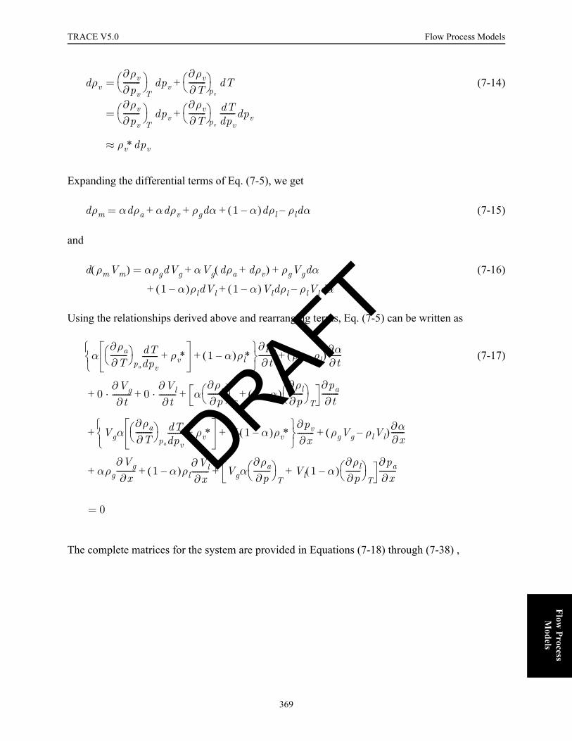
TRACE V5.0 Flow Process Models FOOBAR1234FOOBAR1234FOOBAR1234FOOBAR1234FOOBAR1234FOOBAR1234
Flow Process
Models
(7-14)
Expanding the differential terms of Eq. (7-5), we get
(7-15)
and
(7-16)
Using the relationships derived above and rearranging terms, Eq. (7-5) can be written as
(7-17)
The complete matrices for the system are provided in Equations (7-18) through (7-38) ,
dρv∂ρv∂pv---------⎝ ⎠
⎛ ⎞T
dpv∂ρv∂T---------⎝ ⎠
⎛ ⎞pv
dT+
∂ρv∂pv---------⎝ ⎠
⎛ ⎞T
dpv∂ρv∂T---------⎝ ⎠
⎛ ⎞pv
dTdpv--------dpv
ρv∗dpv≈
+
=
=
dρm αdρa αdρv ρgdα 1 α–( )dρl ρldα–+ + +=
d ρmVm( ) αρgdVg αVg dρa dρv+( ) ρgVgdα
1 α–( )ρldVl 1 α–( )Vldρl ρlVldα–
+ +
+ +
=
α∂ρa∂T---------⎝ ⎠
⎛ ⎞pa
dTdpv-------- ρv∗+ 1 α–( )ρl∗+
⎩ ⎭⎨ ⎬⎧ ⎫∂pv
∂t--------- ρg ρl–( )∂α∂t
-------
0∂Vg∂t
---------- 0∂Vl∂t
--------- α∂ρa∂p---------⎝ ⎠
⎛ ⎞T
1 α–( )∂ρl∂p--------⎝ ⎠
⎛ ⎞T
+∂pa∂t
---------
Vgα∂ρa∂T---------⎝ ⎠
⎛ ⎞pa
dTdpv-------- ρv∗+ Vl 1 α–( )ρv∗+
⎩ ⎭⎨ ⎬⎧ ⎫∂pv
∂x--------- ρgVg ρlVl–( )∂α∂x
-------
αρg∂Vg∂x
---------- 1 α–( )ρl∂Vl∂x
--------- Vgα∂ρa∂p---------⎝ ⎠
⎛ ⎞T
Vl 1 α–( )∂ρl∂p--------⎝ ⎠
⎛ ⎞T
+∂pa∂x---------+
+
+ +
+
+
·+·
+
+
0=
DRAFT
369

Flow Process Models TRACE V5.0
A (7-18)
where
(7-19)
(7-20)
(7-21)
(7-22)
(7-23)
(7-24)
and
A1 1,
ρg ρl– 0 0 A1 5,
0 0 A2 3,
Cα 1 α–( )ρm– 0
0 0 Cα 1 α–( )ρm– A3 4,
0
A4 1,
ρgsg ρlsl– 0 0 A4 5,
α T∂∂ρa
⎝ ⎠⎜ ⎟⎛ ⎞
papvd
dT ρa 0 0 αpa∂
∂ρa
⎝ ⎠⎜ ⎟⎛ ⎞
T
∂pv∂t
---------
∂α∂t-------
∂Vg∂t
------------
∂Vl∂t
----------
∂pg∂t
----------
=
A1 1,
αT∂
∂ρa
⎝ ⎠⎜ ⎟⎛ ⎞
papvd
dT ρv∗+ 1 α–( )ρl∗+=
A1 5,
αp∂
∂ρa
⎝ ⎠⎜ ⎟⎜ ⎟⎛ ⎞
T1 α–( )
p∂
∂ρl
⎝ ⎠⎜ ⎟⎜ ⎟⎛ ⎞
T+=
A2 3,
αρg Cα 1 α–( )ρm+=
A3 4,
1 α–( )ρl Cα 1 α–( )ρm+=
A4 1,
α ρvsv∗– svρv∗ pvddT ρa T∂
∂sa
⎝ ⎠⎜ ⎟⎛ ⎞
pa
sa T∂∂ρa
⎝ ⎠⎜ ⎟⎛ ⎞
pa
+⎝ ⎠⎜ ⎟⎛ ⎞
+ +
1 α–( ) ρlsl∗ sl ρl∗+[ ]+
=
A4 5,
α ρa pa∂∂sa
⎝ ⎠⎜ ⎟⎛ ⎞
Tsa pa∂
∂ρa
⎝ ⎠⎜ ⎟⎛ ⎞
T+ 1 α–( ) ρl p∂
∂sl
⎝ ⎠⎜ ⎟⎛ ⎞
Tsl p∂
∂ρl
⎝ ⎠⎜ ⎟⎛ ⎞
T++=
DRAFT
370

TRACE V5.0 Flow Process Models FOOBAR1234FOOBAR1234FOOBAR1234FOOBAR1234FOOBAR1234FOOBAR1234
Flow Process
Models
B (7-25)
where
(7-26)
(7-27)
(7-28)
(7-29)
(7-30)
(7-31)
(7-32)
B1 1,
B1 2,
αρg 1 α–( )ρl B1 5,
α 0 B2 3,
V– g Cα 1 α–( )ρm α
1 α–( ) 0 Vl Cα 1 α–( )ρm– B3 4,
1 α–( )
B4 1,
B4 2,
αρgsg 1 α–( )ρlsl B4 5,
B5 1,
Vg ρa αρa 0 Vgα pa∂∂ρa
⎝ ⎠⎜ ⎟⎛ ⎞
T
∂pv∂x---------
∂α∂x-------
∂Vg∂x
------------
∂Vl∂x
----------
∂pg∂x
----------
=
B1 1,
Vg T∂∂ρa
⎝ ⎠⎜ ⎟⎛ ⎞
papvd
dT ρv∗+ Vl 1 α–( )ρl∗+=
B1 2,
ρgVg ρlVl–=
B1 5,
Vgα pa∂∂ρa
⎝ ⎠⎜ ⎟⎛ ⎞
TVl 1 α–( ) p∂
∂ρl
⎝ ⎠⎜ ⎟⎛ ⎞
T+=
B2 3,
Vgαρg Vl Cα 1 α–( )ρm+=
B3 4,
Vg Cα 1 α–( )ρm Vl 1 α–( )ρl+=
B4 1,
Vg α ρvsv∗– svρv∗ pvddT ρa T∂
∂sa
⎝ ⎠⎜ ⎟⎛ ⎞
pa
sa T∂∂ρa
⎝ ⎠⎜ ⎟⎛ ⎞
pa
+⎝ ⎠⎜ ⎟⎛ ⎞
+ +
Vl 1 α–( ) ρlsl∗ sl ρl∗+[ ]+
=
B4 2,
Vg ρgsg Vl ρl sl–=
DRAFT
371

Flow Process Models TRACE V5.0
(7-33)
(7-34)
The starred terms are given by the following relationships
(7-35)
(7-36)
and
(7-37)
. (7-38)
With , , and known, all of the thermodynamic partial derivatives used in the aboveequations are obtained by a call to the equation of state package.
The characteristic roots, , of the above system of equations are defined as the roots of the fifth-order polynomial,
determinant (A - B) = 0 . (7-39)
Choking occurs when the signal propagating with the largest velocity relative to the fluid isstationary; that is, the maximum value of the real part of a characteristic root, , is zero.
Eq. (7-39) is extremely difficult to solve analytically. Thus, TRACE obtains the characteristicroots of Eq. (7-39) numerically. This method advantageously maintains generality and facilitatescomputations under different assumptions. The calculational sequence for the TRACE two-phasechoking model is described in Appendix C.
B4 5,
Vg α ρa pa∂∂sa
⎝ ⎠⎜ ⎟⎛ ⎞
Tsa pa∂
∂ρa
⎝ ⎠⎜ ⎟⎛ ⎞
T+ Vl 1 α–( ) ρl p∂
∂sl
⎝ ⎠⎜ ⎟⎛ ⎞
Tsl p∂
∂ρl
⎝ ⎠⎜ ⎟⎛ ⎞
T++=
B5 1,
Vgα T∂∂ρa
⎝ ⎠⎜ ⎟⎛ ⎞
papvd
dT=
ρv∗ pv∂∂ρv
⎝ ⎠⎜ ⎟⎛ ⎞
TT∂
∂ρv
⎝ ⎠⎜ ⎟⎛ ⎞
pv
dTdpv--------+=
sv∗1T----
pv∂∂ev
⎝ ⎠⎜ ⎟⎛ ⎞
TT∂
∂ev
⎝ ⎠⎜ ⎟⎛ ⎞
pv
dTdpv--------+
pv
pv2T
----------pv∂
∂ρv
⎝ ⎠⎜ ⎟⎛ ⎞
TT∂
∂ρv
⎝ ⎠⎜ ⎟⎛ ⎞
pv
dTdpv--------+–=
ρv∗ p∂∂ρl
⎝ ⎠⎜ ⎟⎛ ⎞
T T∂∂ρl
⎝ ⎠⎜ ⎟⎛ ⎞
p
dTdpv--------+=
sl∗1T----
p∂∂el
⎝ ⎠⎜ ⎟⎛ ⎞
T T∂∂el
⎝ ⎠⎜ ⎟⎛ ⎞
p
dTdpv--------+ p
ρl2T
----------p∂
∂ρl
⎝ ⎠⎜ ⎟⎛ ⎞
T T∂∂ρl
⎝ ⎠⎜ ⎟⎛ ⎞
p
dTdpv--------+–=
p pa T
λi
λ
λi re max, ,
DRAFT
372

TRACE V5.0 Flow Process Models FOOBAR1234FOOBAR1234FOOBAR1234FOOBAR1234FOOBAR1234FOOBAR1234
Flow Process
Models
Single-Phase Vapor
The single-phase vapor choked-flow model is based on isentropic expansion of an ideal gas (seeReference 7-8). A throat pressure, , is calculated from the stagnation pressure, , such that
(7-40)
where is the specific-heat ratio. A downstream throat temperature, , is calculated from the
stagnation temperature, , using the ideal-gas relation
(7-41)
When is greater than the saturation temperature at , the fluid flow at the throat is predictedto be superheated by the ideal-gas relations. The continuity equation, in conjunction with theideal-gas relations, yields a fluid choking velocity,
(7-42)
where is the gas constant.
If is less than or equal to the saturation temperature at , then the fluid flow at the throat isnot predicted to be superheated by the ideal-gas relations, and the choking velocity is calculatedusing iterations to maximize mass flux along the isentrope that extends from the superheatedconditions upstream of the throat to the two-phase conditions at the throat. This method assumesthat no delay in condensation occurs as the steam expands to the saturated two-phase state at thethroat.
The calculational sequence for the TRACE single-phase vapor choking model is described inAppendix C.
Transition Regions
Because there is a discontinuity in the sound speed during the transition from liquid to two-phaseflow, the flow during this transition regime must be analyzed carefully. In TRACE, this transition
is handled by linear interpolation between the subcooled ( ) and the two-phase
( ) regimes. The basis for these limits is somewhat arbitrary and comes fromnumerical experimentation designed to identify the values that allow the model to perform most
pe po
pe po2
γ 1+------------⎝ ⎠
⎛ ⎞γ γ 1–⁄
=
γ Te
To
Te To2
γ 1+------------⎝ ⎠
⎛ ⎞=
Te pe
Vge2γγ 1+------------RTo=
R
Te pe
α 1.0≤ 8–×10
α 1.0≥ 5–×10
DRAFT
373

Flow Process Models TRACE V5.0
robustly. The calculational sequence for the TRACE transition region is described in AppendixC.
The transition from the two-phase to the vapor-phase regime is smooth because the two-phasecharacteristic solution approaches the homogeneous equilibrium limit as . Thus, thistransition is made by switching the calculational logic at .
Cell-Center Momentum-Solution Velocities
The velocities obtained from the momentum solution are cell-edge values. However, in order toevaluate stagnation conditions, it is necessary to know the phasic velocities at the cell center. Thistransition between cell edge and cell center is accomplished by averaging the mass flux betweencell edges, such that
(7-43)
and
, (7-44)
where and are the transformed cell-center velocities, and are the steam/gas-
mixture and liquid densities, is the void fraction, and are the liquid and steam/gas-
mixture velocities, and is the cross-sectional flow area. The subscripts and refer toupstream cell-edge and downstream cell-edge quantities, while the subscript refers to cell-center quantities for the particular cell in question. It is assumed that at the upstream face isequal to the upstream cell product value, whereas at the downstream face is taken to be equalto the current cell value because densities and void fractions are normally associated with cell-center rather than with cell-edge positions.
New-Time Choking Velocities.
New-time phasic choking velocities are computed by time-averaging the old-time velocities withthe predicted choking velocities, such that
(7-45)
α 1→α 0.999=
Vgc
12--- ρgα( )
e-Vg e-,A
e- ρgα( )e+V g e+,
Ae++[ ]
ρgcαcAc--------------------------------------------------------------------------------------------------=
Vlc
12--- ρl 1 α–( )( )
e-Vl e-,A
e- ρl 1 α–( )( )e+Vl e+,
Ae++[ ]
ρlc 1 α–( )cAc---------------------------------------------------------------------------------------------------------------------------=
Vgc Vlc ρg ρl
α Vl Vg
A e- e+
cρα
ρα
Vln 1+ 0.1Vle
p 0.9Vln+=
DRAFT
374
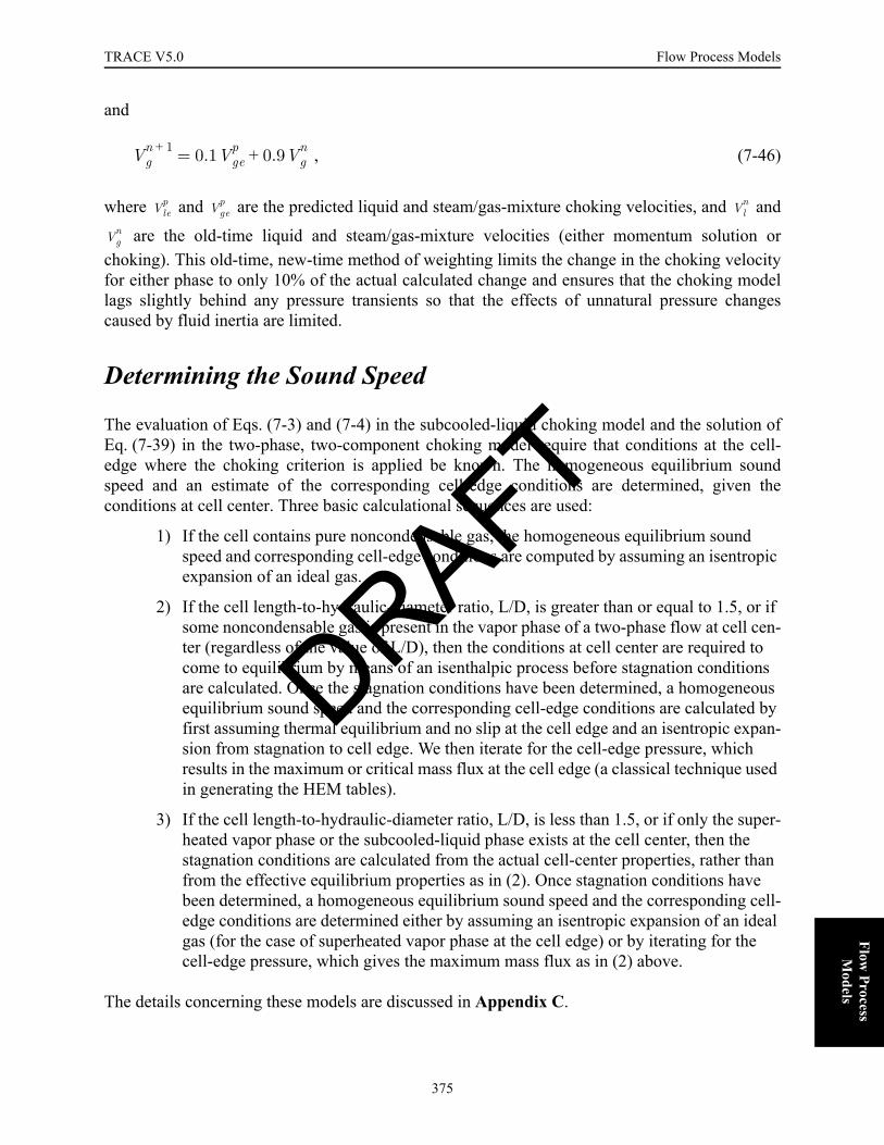
TRACE V5.0 Flow Process Models FOOBAR1234FOOBAR1234FOOBAR1234FOOBAR1234FOOBAR1234FOOBAR1234
Flow Process
Models
and
, (7-46)
where and are the predicted liquid and steam/gas-mixture choking velocities, and and
are the old-time liquid and steam/gas-mixture velocities (either momentum solution orchoking). This old-time, new-time method of weighting limits the change in the choking velocityfor either phase to only 10% of the actual calculated change and ensures that the choking modellags slightly behind any pressure transients so that the effects of unnatural pressure changescaused by fluid inertia are limited.
Determining the Sound Speed
The evaluation of Eqs. (7-3) and (7-4) in the subcooled-liquid choking model and the solution ofEq. (7-39) in the two-phase, two-component choking model require that conditions at the cell-edge where the choking criterion is applied be known. The homogeneous equilibrium soundspeed and an estimate of the corresponding cell-edge conditions are determined, given theconditions at cell center. Three basic calculational sequences are used:
1) If the cell contains pure noncondensable gas, the homogeneous equilibrium sound speed and corresponding cell-edge conditions are computed by assuming an isentropic expansion of an ideal gas.
2) If the cell length-to-hydraulic-diameter ratio, L/D, is greater than or equal to 1.5, or if some noncondensable gas is present in the vapor phase of a two-phase flow at cell cen-ter (regardless of the value of L/D), then the conditions at cell center are required to come to equilibrium by means of an isenthalpic process before stagnation conditions are calculated. Once the stagnation conditions have been determined, a homogeneous equilibrium sound speed and the corresponding cell-edge conditions are calculated by first assuming thermal equilibrium and no slip at the cell edge and an isentropic expan-sion from stagnation to cell edge. We then iterate for the cell-edge pressure, which results in the maximum or critical mass flux at the cell edge (a classical technique used in generating the HEM tables).
3) If the cell length-to-hydraulic-diameter ratio, L/D, is less than 1.5, or if only the super-heated vapor phase or the subcooled-liquid phase exists at the cell center, then the stagnation conditions are calculated from the actual cell-center properties, rather than from the effective equilibrium properties as in (2). Once stagnation conditions have been determined, a homogeneous equilibrium sound speed and the corresponding cell-edge conditions are determined either by assuming an isentropic expansion of an ideal gas (for the case of superheated vapor phase at the cell edge) or by iterating for the cell-edge pressure, which gives the maximum mass flux as in (2) above.
The details concerning these models are discussed in Appendix C.
Vgn 1+ 0.1Vge
p 0.9Vgn+=
Vlep Vge
p Vln
Vgn
DRAFT
375

Flow Process Models TRACE V5.0
Countercurrent FlowCountercurrent flow and CCFL can occur at any location in the reactor system. For instance, inthe case of a reflux-condensation transient associated with a small-break LOCA, countercurrentflow is predicted to exist in the hot leg and in the entrance to the steam-generator inlet plenum. Inthe reactor vessel, CCFL can occur during blowdown as ECC liquid is attempting to fill thedowncomer. During reflood, CCFL can occur at the tie plate, where the upflow of steam preventsor limits the fallback of liquid. This is especially important for those systems that employ upper-plenum ECC injection.
Excluding mass transfer, the accurate prediction of the flow rates is dependent primarily on theinterfacial drag between the phases (which is itself dependent on the accurate prediction of theflow regime). In a given flow system, CCFL usually occurs at a flow-area restriction. Typically,without the use of the CCFL model, TRACE will predict the complete turnaround point (zeroliquid delivery), but overpredict the amount of liquid downflow in the region of countercurrentflow. To improve the prediction in the countercurrent region, a special model exists in TRACEthat allows you to invoke characteristic CCFL correlations at specific locations in the 3DVESSEL component (in the axial direction) or in 1D vertical components.
CCFL in the 3D VESSEL
The CCFL model has been designed primarily for use in the tie-plate region of a PWR. Themechanism for countercurrent flow at this location is very complex. For instance, in a single-bundle experiment, it has been observed that downflow can exist at the periphery of the plate,whereas upflow may occur in the center region. On the average over time, this behavior can bedescribed by a CCFL (or flooding) correlation. CCFL correlations typically provide a superficialmass flux of liquid downflow versus a superficial mass flux of gas upflow. The correlations aredeveloped from the integral over time of the amount of liquid accumulation below the plate for agiven gas-injection rate. The correlation therefore provides a 1D empirical model of the time-averaged multidimensional countercurrent-flow behavior. These correlations are geometry-dependent. For tie plates, the plate thickness, hole diameter (or slot dimensions), number of holes,as well as the type of hardware above and below the tie plate can affect the CCFL characteristics.Rather than try to develop a new mechanistic CCFL model that could predict these complexbehaviors in a variety of geometrical configurations, we decided to make use of the vast amountof correlated data already available. Therefore, the TRACE CCFL model provides you with theoption to implement a CCFL correlation for the specific geometry available and to apply it atspecific locations in the VESSEL component. The input has been generalized so that Wallis (Ref.7-9), Kutateladze (Ref. 7-10), or Bankoff (Ref. 7-11) scaling can be accommodated.
The main point of the CCFL model is that the user supplies the correlation to be used at a specificlocation. Thus, the database is dependent on user input because the correlation constants aredetermined either from experimental data or from estimates based on physical dimensions. If theuser provides a correlation that represents data that are similar to the cell dimensions in geometryand scale, then the code should adequately predict countercurrent flow. Also, CCFL correlations
DRAFT
376
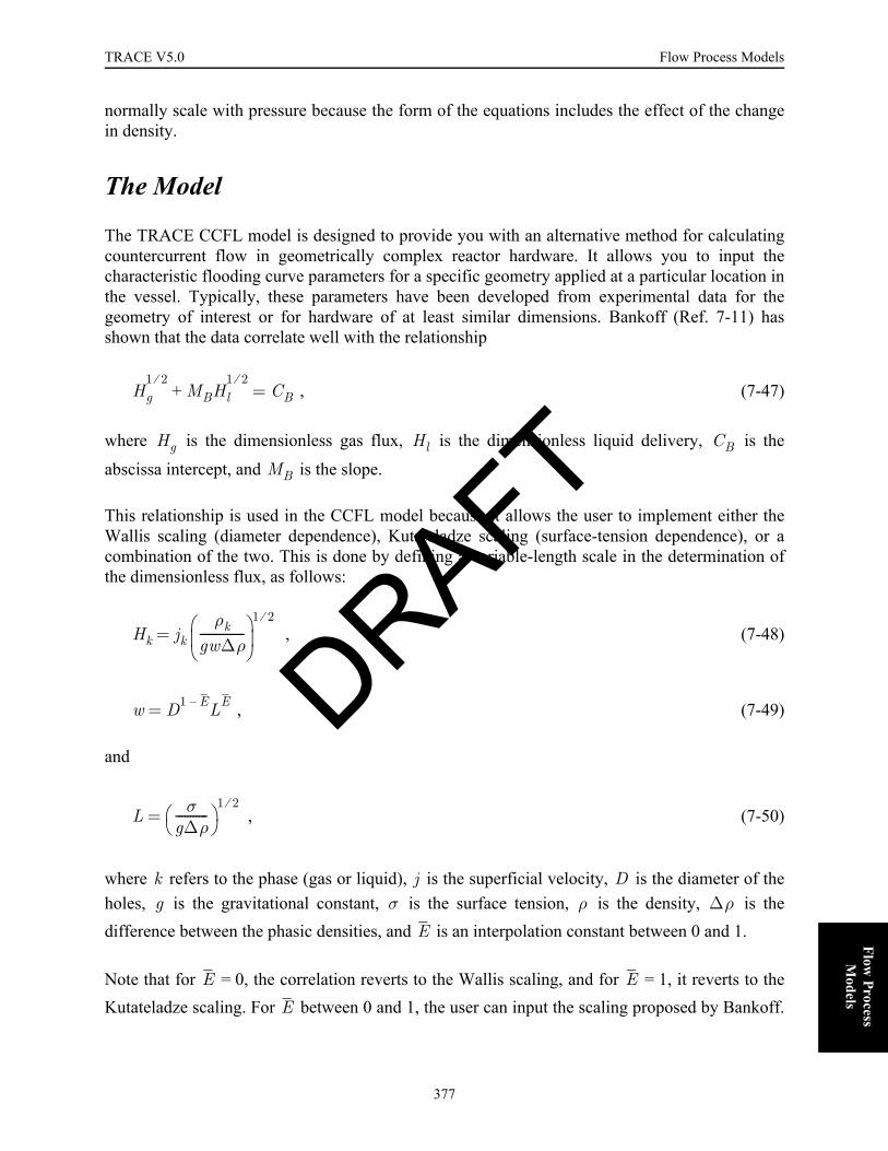
TRACE V5.0 Flow Process Models FOOBAR1234FOOBAR1234FOOBAR1234FOOBAR1234FOOBAR1234FOOBAR1234
Flow Process
Models
normally scale with pressure because the form of the equations includes the effect of the changein density.
The Model
The TRACE CCFL model is designed to provide you with an alternative method for calculatingcountercurrent flow in geometrically complex reactor hardware. It allows you to input thecharacteristic flooding curve parameters for a specific geometry applied at a particular location inthe vessel. Typically, these parameters have been developed from experimental data for thegeometry of interest or for hardware of at least similar dimensions. Bankoff (Ref. 7-11) hasshown that the data correlate well with the relationship
, (7-47)
where is the dimensionless gas flux, is the dimensionless liquid delivery, is the
abscissa intercept, and is the slope.
This relationship is used in the CCFL model because it allows the user to implement either theWallis scaling (diameter dependence), Kutateladze scaling (surface-tension dependence), or acombination of the two. This is done by defining a variable-length scale in the determination ofthe dimensionless flux, as follows:
, (7-48)
, (7-49)
and
, (7-50)
where refers to the phase (gas or liquid), is the superficial velocity, is the diameter of theholes, is the gravitational constant, is the surface tension, is the density, is thedifference between the phasic densities, and is an interpolation constant between 0 and 1.
Note that for = 0, the correlation reverts to the Wallis scaling, and for = 1, it reverts to theKutateladze scaling. For between 0 and 1, the user can input the scaling proposed by Bankoff.
Hg1 2⁄
MBHl1 2⁄
+ CB=
Hg Hl CB
MB
Hk jkρk
gw∆ρ---------------
⎝ ⎠⎜ ⎟⎛ ⎞1 2⁄
=
w D1 E– LE=
L σg∆ρ-----------
⎝ ⎠⎛ ⎞
1 2⁄=
k j Dg σ ρ ∆ρ
E
E E
E
DRAFT
377
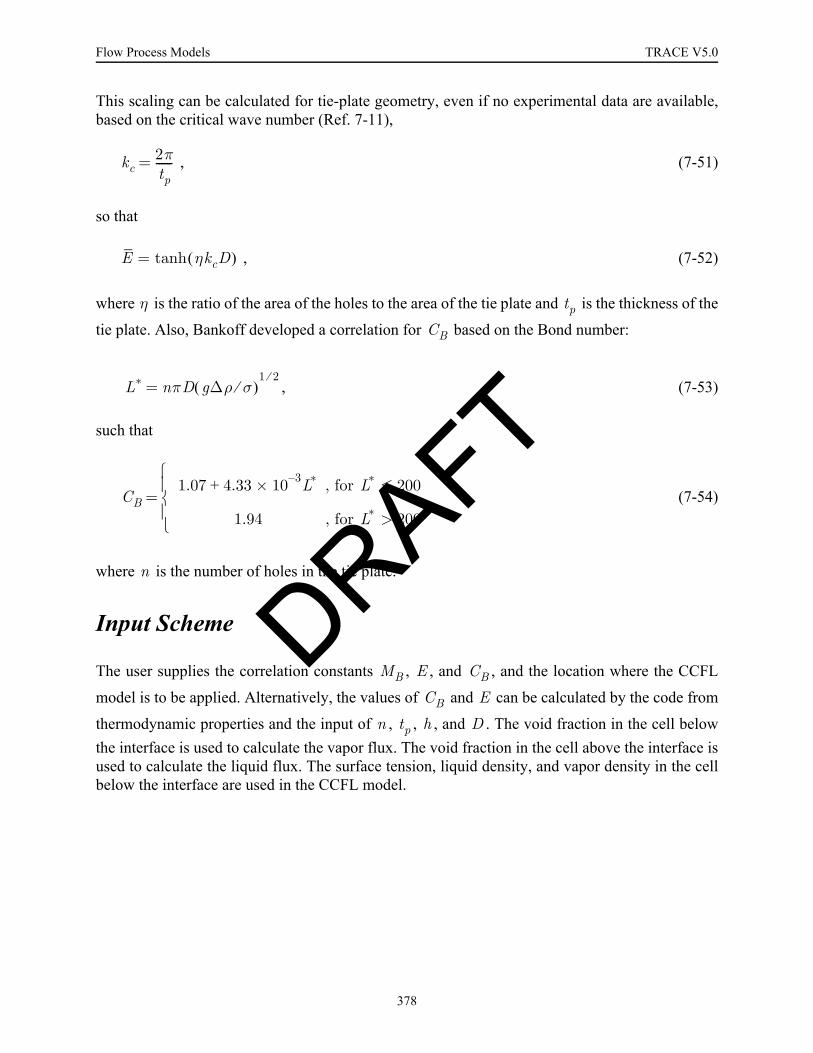
Flow Process Models TRACE V5.0
This scaling can be calculated for tie-plate geometry, even if no experimental data are available,based on the critical wave number (Ref. 7-11),
, (7-51)
so that
, (7-52)
where is the ratio of the area of the holes to the area of the tie plate and is the thickness of the
tie plate. Also, Bankoff developed a correlation for based on the Bond number:
, (7-53)
such that
(7-54)
where is the number of holes in the tie plate.
Input Scheme
The user supplies the correlation constants , , and , and the location where the CCFL
model is to be applied. Alternatively, the values of and can be calculated by the code from
thermodynamic properties and the input of , , , and . The void fraction in the cell belowthe interface is used to calculate the vapor flux. The void fraction in the cell above the interface isused to calculate the liquid flux. The surface tension, liquid density, and vapor density in the cellbelow the interface are used in the CCFL model.
kc2πtp------=
E ηkcD( )tanh=
η tpCB
L* nπD g∆ρ σ⁄( )1 2⁄
=
CB1.07 4.33 10 3–× L*+ , for L* 200≤
1.94 , for L* 200>⎩⎪⎨⎪⎧
=
n
MB E CB
CB E
n tp h D
DRAFT
378

TRACE V5.0 Flow Process Models FOOBAR1234FOOBAR1234FOOBAR1234FOOBAR1234FOOBAR1234FOOBAR1234
Flow Process
Models
Level Tracking
Note – The discussion that follows has been pulled, almost entirely verbatim, from the Ph.D. thesis of Birol Aktas (Ref. 7-24), which was partially funded by NRC. We have taken the liberty to eliminate and/or re-order the presentation of certain concepts so as to fit within the scope and framework of a code theory manual. Where necessary, we also made slight modifications to eliminate typos, improve formatting, fix grammatical issues, change usage of ’TRAC’ to ’TRACE’, etc.
The presence of water levels can severely plague the standard methods of solution to the six-equation model. The use of an average void fraction for a computational volume can lead to anerroneous description of a computational volume when it contains a water level. A short analysisof the initial TRACE simulations of these tests reached a conclusion that such computationalvolumes indeed had two sub-volumes separated by the interface and each of these sub-volumeshad their own distinct flow topology, e.g. the dispersed liquid droplets above the interface and thegas bubbles below. Further conclusion was drawn that for more accurate description of thesedivided computational volumes, regions above and below the interface ought to be treatedseparately requiring the use of separate void fractions inside each region as the outcome ofclosure models strongly depended on the flow regime and the flow regimes were strong functionsof the “cell” void fraction.
Not only the void fractions must be known for the regions above and below the interface but alsothe volumes of each region and the rate at which they change. Only when this additionalinformation is known, one can modify a standard method of solution for the six-equation modelsuch as Semi-Implicit or SETS to accomplish a more accurate description of computationalvolumes with water levels inside them. This strategy of “tracking” to deal with water levelsrequires that the location of a water level, the volumes of regions above and below it, and the voidfractions inside these regions be known at all times.
The idea of tracking water levels is not new. An example is the method which had been developedfor the BWR version of TRAC to track water levels in BWR simulations. This method in TRAC-BWR, which had been applied to the transient simulations of BWRs with some limited success,permitted the use of very large volumes in building computational models of BWR pressurevessels. .
The level tracking method of TRAC-BWR, and of TRACE, consists of two parts: 1) a decisionmaking step to locate and follow the water levels, and 2) modifications to the field equations andclosure models to account for the presence of a water level. The presentation in this section isorganized around these two parts. First, the method of locating the water levels is presented.Modifications to the field equations and the evaluation of closure models then follow. However,there is a third component necessary for a successful level tracking method, mostly overlooked inthe past. This third component is a systematic approach to propagate the water levels across thecell boundaries. The discussions in the following sections present the ideas and approachescritical to a robust method of level tracking. An overview of the first and second components oflevel tracking will be discussed for 1D components to illustrate the level tracking modifications.
DRAFT
379

Flow Process Models TRACE V5.0
A detailed discussion of both 1D and 3D level tracking and details of modifications for the fieldequations, closure model evaluation, and levels crossing cell boundaries will be contained in anAppendix of the manual that will be added in the future.
Level Tracking Method
The search for liquid-gas interfaces is conducted using a series of logical decisions that are basedon empirical observations. Once it is determined that an interface exists inside a computationalvolume, its location inside the volume and its velocity are computed along with the separated sub-volumes. A computational volume that consists of a liquid-gas interface is shown in Figure 7-2. Avoid fraction profile decreasing with increasing height shown in this figure is the simplest casewhere a stratified interface must satisfy either of the following conditions:
(7-55)
(7-56)
The recommended values for , , and are 0.2, 0.005, and 0.7, respectively. Thereare other void fraction profiles, e.g. decreasing with increasing height, reversed void profile aboveand below obstructions, etc... which the liquid-gas interfaces must satisfy different conditions.The void fractions designated for the regions below and above an interface, and the volumes ofthese regions can then be correlated from the computational volume and its void fraction.
Figure. 7-2. A computational volume with the stratified liquid-gas interface
L j∆
x j
αj-
αj+1
αj-1
αj+
αj αj-1– δα>( ) αj+1 αj– ∆αcut>( ) αj+1 αlev>( )∧ ∧
αj αj-1– ∆αcut>( ) αj+1 αj– δα>( ) αj+1 αlev>( )∧ ∧
∆αcut δα αlev
DRAFT
380

TRACE V5.0 Flow Process Models FOOBAR1234FOOBAR1234FOOBAR1234FOOBAR1234FOOBAR1234FOOBAR1234
Flow Process
Models
(7-57)
(7-58)
Subvolumes can be evaluated from Eq. (7-57) and Eq. (7-58).
(7-59)
In a computational volume with constant flow area, the location of the interface can be correlatedfrom Eq. (7-59):
(7-60)
Next, the velocity of the liquid-gas interface is formulated by taking the time derivative ofEq. (7-59) as follows:
(7-61)
(7-62)
In Eq. (7-61), the time derivative of void fractions are first-order approximations. Finally, thelocation of an interface at the end of a timestep can be projected from its location and velocity atthe beginning of a timestep:
(7-63)
When it is determined that a liquid-gas interface exists in a computational volume, an integervariable is set to one to flag its existence. Otherwise, the same variable is set to zero to flag that nointerface is present.
Volj Volj- Volj
++=
Voljαj Volj-αj
- Volj+αj
++=
Volj- αj
+ αj–
αj+ αj
-–------------------- Volj=
Ljαj
+ αj–
αj+ αj
-–------------------- ∆xj=
VL j,
∆xj
αj+ αj
-–-------------------
tddαj
+
tddαj–
Lj
αj+ αj
-–-------------------
tddαj
+
tddαj
-
––=
VL j,n+1 ∆xj
αj+( )
n+1αj
-( )n+1
–----------------------------------------------
αj+( )
n+1αj
+( )n
–∆t
------------------------------------------αj
n+1 αjn–
∆t-------------------------–
Lj
αj+( )
n+1αj
-( )n+1
–----------------------------------------------
αj+( )
n+1αj
+( )n
–∆t
------------------------------------------αj
-( )n+1
αj-( )
n–
∆t--------------------------------------––
=
Ljn+1 Lj
n ∆t VL j,n+1+=
DRAFT
381
Flow Process Models TRACE V5.0
(7-64)
Modifications To The Field Equations
Once it is determined that a liquid-gas interface is present in a computational cell, a new variable,, is defined to specify the distance between the liquid-gas interface and the cell boundaries. A
second variable, , is defined to specify the void fraction of the two-phase fluid convectedacross the boundaries between two adjacent volumes.
(7-65)
(7-66)
(7-67)
In the above equations, is the void fraction at a boundary defined as an average of voidfractions computed for the cells adjacent to a boundary.
Mass and Energy Equations
When a liquid-gas interface is present in a computational cell, its presence must be accounted forby the terms that describe the flux of mass and energy across the cell boundaries. The flux terms
λj1 , for 0 Lj ∆xj< <
0 , otherwise⎩⎪⎨⎪⎧
=
λE
αE
λE j+1/2,
Lj+1 , if λj+1= 1
Lj ∆xj– , if λj= 1
0 , otherwise⎩⎪⎨⎪⎧
=
αE j-1/2,
αj- , if λ
E j-1/2,0>
αj-1+ , if λ
E j-1/2,0<
α⟨ ⟩ j-1/2 , if λE j-1/2,=0
⎩⎪⎪⎪⎨⎪⎪⎪⎧
=
αE j+1/2,
αj+1- , if λ
E j+1/2,0>
αj+ , if λ
E j+1/2,0<
α⟨ ⟩ j+1/2 , if λE j+1/2,=0
⎩⎪⎪⎪⎨⎪⎪⎪⎧
=
α⟨ ⟩
DRAFT
382

TRACE V5.0 Flow Process Models FOOBAR1234FOOBAR1234FOOBAR1234FOOBAR1234FOOBAR1234FOOBAR1234
Flow Process
Models
used in the regular solution schemes shown in Equations (1-101), (1-104), (1-105), and (1-106)use an average of properties from adjacent cells as an approximation for the state properties,which are defined and calculated at cell centers by definition, across the cell boundary. Once it isdetermined that a liquid-gas interface is present adjacent to a cell boundary, averaging of theproperties at the boundary must account for the presence of the interface. Accounting for thepresence of the interface is accomplished by redefining the flow area at the cell boundary in thefollowing redefined flux terms:
(7-68)
(7-69)
(7-70)
(7-71)
(7-72)
(7-73)
where the new definition of flow area in the gas and liquid terms, i.e. and ,
accounts for the presence of an interface in either cell adjacent to the boundary:
(7-74)
φg j+1/2,
αρg⟨ ⟩ j+1/2n A
g j+1/2,α V
g j+1/2,n+1=
φl j+1/2,
1 α–( )ρl⟨ ⟩ j+1/2n A
l j+1/2,α V
l j+1/2,n+1=
ζg j+1/2,
αρgeg⟨ ⟩ j+1/2n A
g j+1/2,α V
g j+1/2,n+1=
ζl j+1/2,
1 α–( )ρlel⟨ ⟩ j+1/2n A
l j+1/2,α V
l j+1/2,n+1=
ωg j+1/2,
α⟨ ⟩ j+1/2n A
g j+1/2,α V
g j+1/2,n+1=
ωl j+1/2,
1 α–⟨ ⟩ j+1/2n A
l j+1/2,α V
l j+1/2,n+1=
Ag j+1/2,α A
l j+1/2,α
Ag j+1/2,α
Aj+1/2
αE j+1/2,
αj---------------------- , if λ
E j+1/2,0<⎝ ⎠
⎛ ⎞ and Vg j+1/2,
0>⎝ ⎠⎛ ⎞
Aj+1/2
αE j+1/2,
αj+1---------------------- , if λ
E j+1/2,0>⎝ ⎠
⎛ ⎞ and Vg j+1/2,
0<⎝ ⎠⎛ ⎞
Aj+1/2 , otherwise⎩⎪⎪⎪⎪⎨⎪⎪⎪⎪⎧
=
DRAFT
383

Flow Process Models TRACE V5.0
(7-75)
The above equations redefine the flux terms in the mass and energy equations of the basic step,i.e. Equations (1-141), (1-144), (1-145), and (1-146), accurately in terms of void fractions aboveand below a water level. However, these corrections to the flux terms in the basic step equationsdo not work for the flux terms in the stabilizer step equations, i.e. Equations (1-149), (1-152), (1-
156), and (1-157) as the flux terms in these equations are formulated in terms of from the
basic step, not of the previous time step. The following equations further adjust the “phasic”flow areas so that the flux terms in the stabilizer step equations remain consistent with thesolution to the basic step equations.
(7-76)
(7-77)
Redefining the macroscopic quantities that are convected across the cell boundaries in terms ofthe void fractions above and below an interface curtails the otherwise inadvertent flux ofquantities based on cell average void fraction. The modifications above are necessary but notsufficient for a successful method of level tracking. Additional considerations must be given tothe other terms which make up the fluxes, i.e. liquid and gas velocities.
Al j+1/2,α
Aj+1/2
1 αE j+1/2,
–
1 α– j------------------------------- , if λ
E j+1/2,0<⎝ ⎠
⎛ ⎞ and Vl j+1/2,
0>⎝ ⎠⎛ ⎞
Aj+1/2
1 αE j+1/2,
–
1 αj+1–------------------------------- , if λ
E j+1/2,0>⎝ ⎠
⎛ ⎞ and Vl j+1/2,
0<⎝ ⎠⎛ ⎞
Aj+1/2 , otherwise⎩⎪⎪⎪⎪⎨⎪⎪⎪⎪⎧
=
αn+1
αn
Ag j+1/2,α
Ag j+1/2,α αj
n
αjn+1
------------ if λE j+1/2,
0<⎝ ⎠⎛ ⎞ and V
g j+1/2,0>⎝ ⎠
⎛ ⎞,
Ag j+1/2,α αj+1
n
αj+1n+1
------------ if λE j+1/2,
0>⎝ ⎠⎛ ⎞ and V
g j+1/2,0<⎝ ⎠
⎛ ⎞,
⎩⎪⎪⎪⎨⎪⎪⎪⎧
→
Al j+1/2,α
Al j+1/2,α 1 α– j
n( )
1 α– jn+1
( )-------------------------- if λ
E j+1/2,0<⎝ ⎠
⎛ ⎞ and Vl j+1/2,
0>⎝ ⎠⎛ ⎞,
Al j+1/2,α 1 α– j+1
n( )
1 αj+1n+1
–( )-------------------------- if λ
E j+1/2,0>⎝ ⎠
⎛ ⎞ and Vl j+1/2,
0<⎝ ⎠⎛ ⎞,
⎩⎪⎪⎪⎨⎪⎪⎪⎧
→
DRAFT
384
TRACE V5.0 Flow Process Models FOOBAR1234FOOBAR1234FOOBAR1234FOOBAR1234FOOBAR1234FOOBAR1234
Flow Process
Models
Momentum Equations
The phase velocities at time level n+1 are expressed as linear functions of pressure changes at theadjacent computational volumes:
(7-78)
(7-79)
Equations (7-78) and (7-79) are substituted into Eqs. (7-68) to (7-73) eliminating the velocities asunknowns from the flux terms. Thus, the flux terms consists of two components before the
iterative solution begins: 1) the known portion in terms of the tilde fluid velocities ( ), and
2) the variable portion in terms of the unknown changes in pressures ( ). The flux quantitiesmodified by Eqs. (7-74) and (7-75) multiply both the known and the variable portions of fluxterms. It should not be overlooked that the product of the tilde velocities and modified fluxquantities will be inconsistent unless the momentum equations, i.e. Eq. (1-99) and Eq. (1-100),are also modified to account for the presence of liquid-gas interfaces.
This subtle detail pertinent to Eqs. (1-99) and (1-100) deserves further clarification. Equations(1-99) and (1-100) balance the fluid momentum across a staggered control volume for liquid andgas fields, i.e. the control volume drawn with thick dotted lines in Figure 7-3 that stretches fromthe center of cell to the center of cell . The use of staggered control volumes allows theexpression of the net force due to pressure drop across the fluid enclosed by the staggered volumesimply as without the need for any further approximation. In the meantime, othervariables such as fluid density and void fraction in Eq. (1-99) and Eq. (1-100) are approximationssince these variables are defined at cell centers. From the balance of momentum across astaggered cell, Eq. (1-99) and Eq. (1-100) are formulated for the liquid and gas velocities. Later,the product of these velocities and the flux quantities at cell boundaries, depicted by the arrowslocated at j+½ in Figure 7-3, define the flux of mass and energy across the cell boundary. Asolution with the standard upstream donor method defines the flux quantitities at cell boundariesas an average of quantities from the adjacent cells. This picture must be revisited when the fluidenclosed by the staggered control volume is no longer uniform and it consists of two regionsdivided by an interface.
Vj+1/2n+1 Vj+1/2
n+1
Pj+1n+1∂
∂Vj+1/2n+1
δPj+1Pj
n+1∂
∂Vj+1/2n+1
δPj+
⎩ ⎭⎪ ⎪⎨ ⎬⎪ ⎪⎧ ⎫
i∑+=
Vj-1/2n+1 Vj-1/2
n+1
Pjn+1∂
∂Vj-1/2n+1
δPjPj-1
n+1∂
∂Vj-1/2n+1
δPj-1+
⎩ ⎭⎪ ⎪⎨ ⎬⎪ ⎪⎧ ⎫
i∑+=
Vj+1/2n+1
δPji
j j 1+
Pj-1 Pj–
DRAFT
385
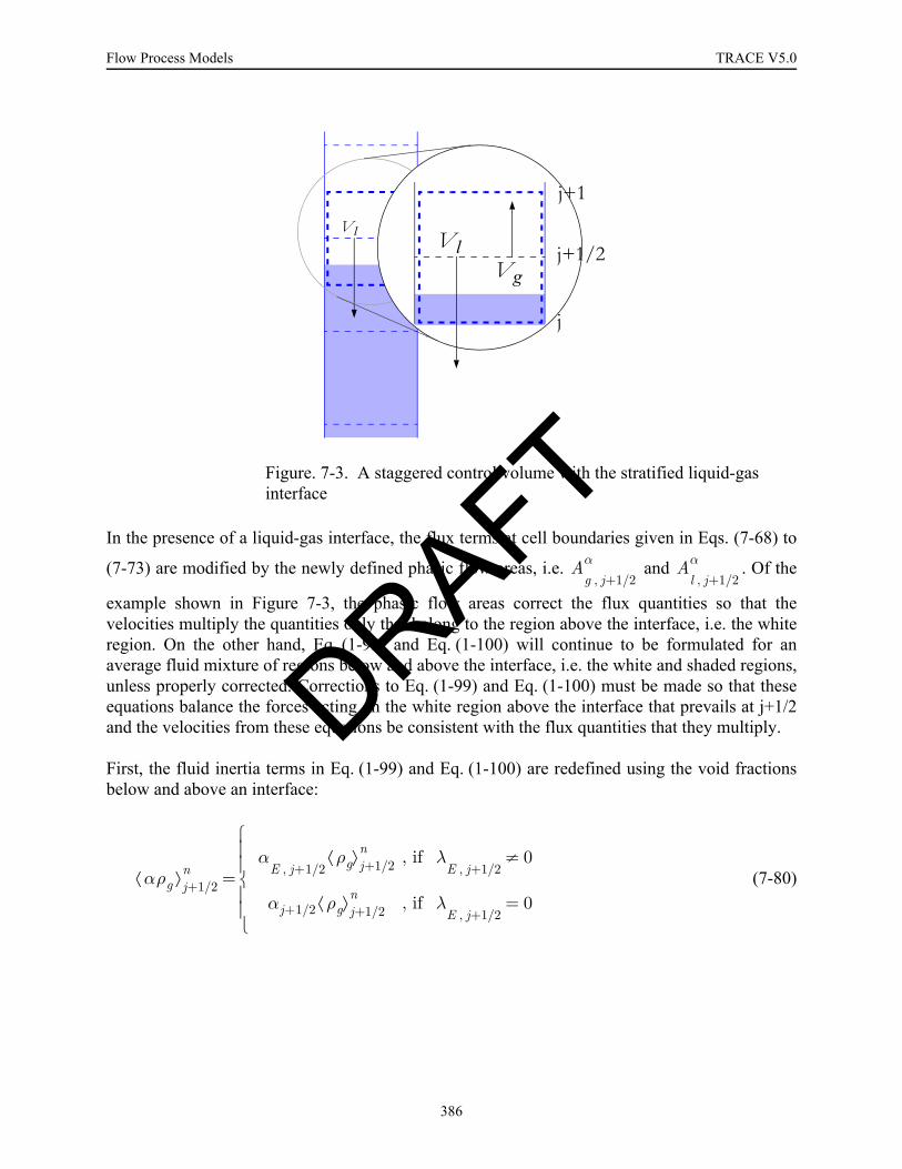
Flow Process Models TRACE V5.0
In the presence of a liquid-gas interface, the flux terms at cell boundaries given in Eqs. (7-68) to
(7-73) are modified by the newly defined phasic flow areas, i.e. and . Of the
example shown in Figure 7-3, the phasic flow areas correct the flux quantities so that thevelocities multiply the quantities only that belong to the region above the interface, i.e. the whiteregion. On the other hand, Eq. (1-99) and Eq. (1-100) will continue to be formulated for anaverage fluid mixture of regions below and above the interface, i.e. the white and shaded regions,unless properly corrected. Corrections to Eq. (1-99) and Eq. (1-100) must be made so that theseequations balance the forces acting on the white region above the interface that prevails at j+1/2and the velocities from these equations be consistent with the flux quantities that they multiply.
First, the fluid inertia terms in Eq. (1-99) and Eq. (1-100) are redefined using the void fractionsbelow and above an interface:
(7-80)
Figure. 7-3. A staggered control volume with the stratified liquid-gas interface
j+1/2
j-1/2
j
j+1
VlVg j+1/2
j
j+1
VlVg
Ag j+1/2,α A
l j+1/2,α
αρg⟨ ⟩ j+1/2n
αE j+1/2,
ρg⟨ ⟩ j+1/2n , if λ
E j+1/2,0≠
αj+1/2 ρg⟨ ⟩ j+1/2n , if λ
E j+1/2,0=
⎩⎪⎪⎨⎪⎪⎧
=
DRAFT
386
TRACE V5.0 Flow Process Models FOOBAR1234FOOBAR1234FOOBAR1234FOOBAR1234FOOBAR1234FOOBAR1234
Flow Process
Models
(7-81)
Second, the pressure gradient term in Eq. (1-99) and Eq. (1-100) is redefined as
(7-82)
where the correction term to account for the presence of a liquid-gas interface is given by thefollowing equation.
(7-83)
It should be noted that Eq. (7-83) yields an accurate pressure drop from the interface to the cellboundary not only due to the hydrostatic head of fluid but also due to the fluid accelaration. Thisdetail should not be overlooked and it is important for situations in which an interface accelarates.It should also be emphasized that Eq. (7-83) yields to the weight of the fluid below the interfacebetween the interface and the cell boundary in the hydrostatic limit, i.e. when there is no pressure
drop due to fluid accelaration .
Third, the gradients of liquid and gas velocities across the cell boundary are set to zero based onan assumption that the changes in fluid velocity across the interface will not contribute to thepressure drop across the staggered control volume. For example, the gas bubbles that reach theliquid-gas interface rise at a terminal velocity. The velocity of gas escaping from the interface isgenerally much smaller than the terminal rise velocity of gas bubbles below the interface.However, this sudden slowdown of gas across the interface, which is due to continuity, should notcause additional pressure changes across the staggered cell. Similarly, the liquid dropletsentrained into the region above the interface may have higher velocity than the continuous liquidregion below the interface. Any additional pressure drop due to this change of liquid velocityacross the staggered cell is incorrect, too. Therefore, the velocity gradient of a field at any cellboundary is set to zero when a liquid-gas interface is present in the upstream direction of that
1 α–( )ρl⟨ ⟩ j+1/2n
1 α–E j+1/2,
( ) ρl⟨ ⟩ j+1/2n , if λ
E j+1/2,0≠
1 α– j+1/2( ) ρl⟨ ⟩ j+1/2n , if λ
E j+1/2,0=
⎩⎪⎪⎨⎪⎪⎧
=
x∂∂P
j+1/2
n 1+ Pj+1n 1+ Pj
n 1+– PL j+1/2,
δ+
∆xj+1/2-----------------------------------------------------------------=
PL j+1/2,
δ
0.5∆xj+1 Lj+1–( )x∂
∂P
j-1/2
n 1+
, if Lj+1 0.5∆xj+1<
0.5∆xj Lj–( )x∂
∂P
j-3/2
n 1+
, if Lj 0.5∆xj>
0 , otherwise⎩⎪⎪⎪⎪⎨⎪⎪⎪⎪⎧
=
t∂∂V 0=
DRAFT
387

Flow Process Models TRACE V5.0
field. The correction to the gradients of liquid and gas velocities are formulated into EquationsEq. (1-99) and Eq. (1-100) as follows:
when (7-84)
when (7-85)
As the level tracking method and the necesary modifications to the field equations describedEq. (7-55) to Eq. (7-85) are incorporated, numerical experiments presented must be simulated totest the method and the modifications to the field equations.
Corrections to Evaluation of the Closure Models
The modifications to the field equations and the extra measures taken to ensure that the waterlevels cross the cell boundaries without harming the solution are not sufficient alone for asuccessful level tracking method. Although not discussed in the previous sections, a correction isnecessary to the definition of the interfacial drag coefficient in terms of fluid properties at a cellboundary when a liquid-gas interface is present in either cell adjacent to a boundary. Thiscorrection to the interfacial drag coefficient is explained here along with another correction to theinterfacial heat transfer coefficient.
Interfacial Drag
Let us first consider the interfacial drag coefficient, in Eq. (4-1). This coefficient relates thedrag force between the separated field to the relative velocity of one field to another. Therefore, itis a strong function of the flow regime The void fraction that is used to determine the flow regimefor any given staggered cell (see Figure 7-3) is an average of void fractions from half-cells thatmake up the staggered cell. As emphasized in discussions on modifications to the momentumequations, the use of an average void fraction for the entire staggered is not consistent with thecorrections made to the flux terms of conservation equations. The conclusion from thesediscussions is that the balance of forces acting on the fluid should represent the conditionsprevailing at cell boundaries, i.e. the center of staggered cell. In view of this conclusion, the
x∂∂Vl
j+1/2
n
0=λ
E j+1/2,0<⎝ ⎠
⎛ ⎞ and Vl j+1/2,n 0>⎝ ⎠
⎛ ⎞
λE j+1/2,
0>⎝ ⎠⎛ ⎞ and V
l j+1/2,n 0<⎝ ⎠
⎛ ⎞⎩⎪⎪⎨⎪⎪⎧
x∂∂Vg
j+1/2
n
0=λ
E j+1/2,0<⎝ ⎠
⎛ ⎞ and Vg j+1/2,n 0>⎝ ⎠
⎛ ⎞
λE j+1/2,
0>⎝ ⎠⎛ ⎞ and V
g j+1/2,n 0<⎝ ⎠
⎛ ⎞⎩⎪⎪⎨⎪⎪⎧
Ci
DRAFT
388

TRACE V5.0 Flow Process Models FOOBAR1234FOOBAR1234FOOBAR1234FOOBAR1234FOOBAR1234FOOBAR1234
Flow Process
Models
interfacial drag coefficient in Eq. (4-1) is evaluated in terms of fluid conditions that prevail at thecell boundary when a liquid-gas interface is present in either of cells adjacent to the boundary.
(7-86)
Figure 7-4 shows the interface drag coefficients at cell boundaries (i.e. cell faces) along the testpipe of the single-phase rising and falling test. The sharp change in the drag coefficient isexpected as the water level crosses the cell boundaries. It should be noted here that it is a commonpractice among the methods like semi-implicit to impose limits on the rate at which dragcoefficients change. Such limits are set to prevent numerical instabilities due to explicit nature ofthese coefficients. In the case of an interface crossing the cell boundary, however, no limit shouldbe imposed on the interfacial drag coefficient since a sharp change is expected and the remainderof equations are already preconditioned to account for sharp changes and to remain stable.Contrary to the other cases, imposing any such limit renders the solution unstable in this case.
The interfacial drag coefficients at cell faces along the test pipe of the two-phase rising and fallingtest exhibit sharp changes, as expected, as the mixture level crosses the cell boundaries. Inaddition to the expected sharp changes, the interfacial drag coefficients in Figure 7-5 also showhow strongly the drag coefficient depends on the void fraction that prevails at the cell boundaryalong with the relative motion of fields against each other. In this figure, the decreasing dragcoefficient at a cell boundary realizes the slight depression of void fraction in the adjacent cells, asis also shown later in Figure 7-13, as the column of bubbly liquid and gas mixture rises above a
Figure. 7-4. Interfacial drag coefficients at cell boundaries of the single-phase fill and drain test (simulated with the level tracking method)
0 2 4 6 8 10Time (s)
0
500
1000
1500
2000
Dra
g C
oef (
kg/m
4)face 5face 6face 7face 8
Ci j+1/2,
C αE j+1/2,
( ) , if λE j+1/2,
0≠
C α⟨ ⟩ j+1/2( ) , if λE j+1/2,
0=⎩⎪⎨⎪⎧
=
DRAFT
389

Flow Process Models TRACE V5.0
cell boundary. This behavior is physically sensible since the void fraction of a bubbly liquid-gasmixture is expected to decrease under an increasing weight of the rising mixture column.
Interfacial Heat and Mass Transfer
The closure model for the interfacial heat transfer (IHT) between the liquid and gas fields mustaccount for the presence of water levels in computational cells. A brief description of the IHTmodel in TRACE is therefore appropriate here before discussing how the IHT model should beadjusted. The following two equations describe the heat transfer to and from liquid and gas at thephase interface
(7-87)
(7-88)
where
Figure. 7-5. Interfacial drag coefficients at cell boundaries of the two-phase fill and drain test (simulated with the level tracking method)
0 2 4 6 8 10Time (s)
0
500
1000
1500
2000
2500
3000
Dra
g C
oef (
kg/m
4) face 5face 6face 7face 8
qg qig qdg+=
PsP------HCHTI Tg Tsv–( )
PaP------HCHTA Tg Tl–( )+=
ql qil qdl+=
HALVE Tl Tsv–( ) HALV Tl Tsat–⟨ ⟩†+[ ]PaP------HCHTA Tl Tg–( )+=
DRAFT
390

TRACE V5.0 Flow Process Models FOOBAR1234FOOBAR1234FOOBAR1234FOOBAR1234FOOBAR1234FOOBAR1234
Flow Process
Models
. (7-89)
Eq. (7-87) assumes that the gas field is a homogeneous mixture of water vapor andnoncondensable gas in thermodynamic equilibrium. The first term in Eq. (7-87) accounts for heattransfer to or from the interface ( ) and is converted to or released as latent heat through phasechange. The second term in Eq. (7-87) is the direct sensible heat exchange between the liquid andthe gas fields. Similarly, the first term in Eq. (7-88) corresponds to the sensible heat transferred toor from the interface, which is converted to or released as latent heat. The second term inEq. (7-88) is the direct sensible heat exchange between the liquid and the gas fields. It should benoted that the liquid to interface has two heat transfer coefficients, and , for
condensation and evaporation. Evaporation occurs if and flashing occurs if
. Equations (7-87) and (7-88) are added to calculate the total rate of heat exchange at
the phase interface where the direct sensible heat transfer terms, and , cancel out.
(7-90)
When there is a water level inside a computational cell, the IHT coefficients must be determinedfor each region above and below the level along with the coefficients that describe the heattransfer at the level as follows:
(7-91)
. (7-92)
The heat transfer coefficients for regions above and below the interfaces can be easily determinedusing the same procedures that apply to an entire computational cells. However, it should benoted that the field temperatures are assumed identical above and below the interface. This is anassumption which may lead to significant errors. Another area of concern is the description heattransfer at the level. In the presence of a strong condensation, the temperature of stratified liquidnear the level may be very close to the saturation temperature, and thus, create a resistance tofurther condensation. As this may sound like a subtle detail, it is a situation which should beconsidered very carefully and accounted for by the IHT terms “from” and “to” the saturation
interface at the water level, i.e. and . For the purpose of this discussion, these two termswill be determined using TRACE’s special treatment for the computational volumes thatrepresent the accumulator or pressurizer of a nuclear plant while it is noted that evaluating thesetwo terms accurately requires an investigation of its own.
Tl Tsat–⟨ ⟩†0 if Tl Tsat≤
Tl Tsat– if Tl Tsat>⎩⎪⎨⎪⎧
=
qig
HALV HALVE
Tsv Tl Tsat< <
Tl Tsat>
qdg qdl
Vol hfg Γi· qig qil+=
qg qig - qdg
-+( ) qigL qdg
L+( ) qig+ qdg
++( )+ +=
ql qil - qdl
-+( ) qilL qdl
L+( ) qil+ qdl
++( )+ +=
qigL qil
L
DRAFT
391

Flow Process Models TRACE V5.0
Numerical ExperimentsAs the level tracking method and the necesary modifications to the field equations describedEq. (7-55) to Eq. (7-85) are incorporated, numerical experiments presented must be simulated totest the method and the modifications to the field equations. A thorough testing is critical to asuccessful implementation of the level tracking method. Several simple problems were run toshow the problems with the regular solution scheme and how level tracking improves the results.
Fill and Drain Test
A schematic diagram of the test problem is shown in Figure 7-7. The model consists of a verticalpipe with 1.0 m2 axial flow area and 10.0 m height. A “T” branch with 0.5 m2 axial flow area and3.0 m height is connected to the bottom of the test pipe. There are two variations to this testproblem. In the first case, liquid water is injected, at the side entry of the “T” branch, to raise thelevel of the liquid column and then withdrawn to let the level drop back to its starting location. Inthe second case, air is injected, at the bottom entry of the “T” branch, to maintain a steady mixtureof liquid water and air under the standard room temperature and pressure conditions. Again,liquid water is first injected to raise the level of the mixture, and then withdrawn to let the leveldrop back to its starting location. The injection and withdrawal of liquid water in both cases at1.0 m3/s moves the level across one computational volume in every second.
Figure. 7-6. Interfacial HT terms designated for a computational volume with the stratified liquid-gas interface
j
j+1
jq+
q-
qL
DRAFT
392
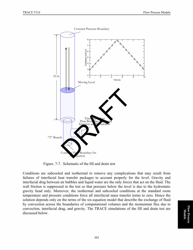
TRACE V5.0 Flow Process Models FOOBAR1234FOOBAR1234FOOBAR1234FOOBAR1234FOOBAR1234FOOBAR1234
Flow Process
Models
Conditions are subcooled and isothermal to remove any complications that may result fromfailures of interfacial heat transfer packages to account properly for the level. Gravity andinterfacial drag between air bubbles and liquid water are the only forces that act on the fluid. Thewall friction is suppressed in the test so that pressure below the level is due to the hydrostaticgravity head only. Moreover, the isothermal and subcooled conditions at the standard roomtemperature and pressure conditions force all interfacial mass transfer terms to zero. Hence thesolution depends only on the terms of the six-equation model that describe the exchange of fluidby convection across the boundaries of computational volumes and the momentum flux due toconvection, interfacial drag, and gravity. The TRACE simulations of the fill and drain test arediscussed below.
Figure. 7-7. Schematic of the fill and drain test
0 2 4 6 8 10Time (s)
2
3
4
5
6
7
8
Col
laps
ed L
evel
(m)
“T” Branch
Moving Level
Constant Pressure Boundary
Time-dependent
Injection and Withdrawal
Constant Flow Boundary for
Flow Boundary for Liquid
Air Injection
10 m
DRAFT
393

Flow Process Models TRACE V5.0
Shown in Figure 7-8 is the computational model that represents the test pipe, made of ten equalcomputational volumes. Henceforth, the computational volumes will also be referred to as “cells.”
This test problem was simulated using the SETS method of TRACE with the standard upstreamdonor method. As shown in Figure 7-8, the collapsed water level, which is given by
, (7-93)
Figure. 7-8. Schematic of the fill and drain test simulated using one-dimensional equations
1
2
3
4
5
6
7
8
9
10
“T” Branch
Moving Level
Constant Pressure Boundary
Time-dependent
Injection and Withdrawal
Constant Flow Boundary for
Flow Boundary for Liquid
Air Injection
HC t( ) 1 αi t( )–[ ]∆xii 1=
N
∑=
DRAFT
394

TRACE V5.0 Flow Process Models FOOBAR1234FOOBAR1234FOOBAR1234FOOBAR1234FOOBAR1234FOOBAR1234
Flow Process
Models
(where is the total number of computational cells) is rising and falling back to its startinglocation at a steady rate. The rising front is expected to fill the computational volumes at a steadyrate starting from the bottom of the pipe and move to the next volume above once a volume is fullof liquid water. The SETS solution of TRACE with the standard upstream donor method fails topredict this expected behavior of cell void fractions as the water level rises. A plot of voidfractions in Figure 7-9 shows that the liquid front moves to the next volume above, before thevolume is fully liquid water, trapping a gas bubble behind. This distorted picture of the risingliquid front repeats itself as the water is drained from the test pipe and the water level drops backto its starting location. The liquid front is smeared over several volumes as the descending liquidfront leaves significant amount of liquid left behind in its tail. Due to smearing of the liquid front,the “predicted” cell pressures (shown in Figure 7-10) below the moving liquid front do not exhibitthe expected behavior as well, i.e. a steady change proportional to the height of the rising andfalling water level. Instead, the cell pressures below the water level increase and decreasesporadically indicating sudden acceleration and deceleration of the fluid, a behavior which isabsolutely numerical in nature. Figure 7-11 and Figure 7-12 show that the SETS method with thestandard donor method continues to suffer severely from similar difficulties when the fluid belowthe moving liquid front is a mixture of air and liquid water.
The two-phase rising and falling level test also shows none of the troubles that were reported inthe previous section. For example, the troubling cell void fractions from 0 to 5 seconds seen inFigure 7-11 are no longer present in Figure 7-15. Previously, the cell void fractions approachedto zero which was well below the expected value of void fraction for the bubbly mixture of liquidand air simulated in this experiment. The cell pressures reported previously for the same test inFigure 7-12 suffered from spike changes and oscillations as the water level crossed the cellboundaries. The cell pressures shown in Figure 7-16 are clean from these spike changes andoscillations. It should be noted that the sudden drop in cell pressures as the bubbly mixture of
Figure. 7-9. Void fractions of the single-phase fill and drain test (simulated with the standard method of solution)
N
0 2 4 6 8 10Time (s)
0
0.2
0.4
0.6
0.8
1
Voi
d Fr
actio
n
cell 4cell 5cell 6cell 7cell 8
DRAFT
395

Flow Process Models TRACE V5.0
liquid and gas reverses direction is due to the fluid acceleration in the opposite direction ofgravity.
Oscillating Manometer
The U-tube manometer in this test consists of gas and liquid with the liquid forming equalcollapsed water levels in each arm. Initially, the liquid slug has a uniform velocity and noacceleration. The top of manometer arms are open to the standard room temperature and pressure
Figure. 7-10. Pressures of the single-phase fill and drain test (simulated with the standard method of solution)
Figure. 7-11. Void fractions of the two-phase fill and drain test (simulated with the standard method of solution)
0 2 4 6 8 10Time (s)
100
110
120
130
140
150
Pre
ssur
e (K
Pa)
cell 4cell 5cell 6cell 7cell 8
0 2 4 6 8 10Time (s)
0
0.2
0.4
0.6
0.8
1
Voi
d Fr
actio
n
cell 4cell 5cell 6cell 7cell 8DRAFT
396
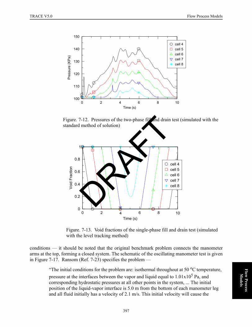
TRACE V5.0 Flow Process Models FOOBAR1234FOOBAR1234FOOBAR1234FOOBAR1234FOOBAR1234FOOBAR1234
Flow Process
Models
conditions — it should be noted that the original benchmark problem connects the manometerarms at the top, forming a closed system. The schematic of the oscillating manometer test is givenin Figure 7-17. Ransom (Ref. 7-23) specifies the problem —
“The initial conditions for the problem are: isothermal throughout at 50 oC temperature, pressure at the interfaces between the vapor and liquid equal to 1.01x10⁵ Pa, and corresponding hydrostatic pressures at all other points in the system, ... The initial position of the liquid-vapor interface is 5.0 m from the bottom of each manometer leg and all fluid initially has a velocity of 2.1 m/s. This initial velocity will cause the
Figure. 7-12. Pressures of the two-phase fill and drain test (simulated with the standard method of solution)
Figure. 7-13. Void fractions of the single-phase fill and drain test (simulated with the level tracking method)
0 2 4 6 8 10Time (s)
100
110
120
130
140
150
Pre
ssur
e (K
Pa)
cell 4cell 5cell 6cell 7cell 8
0 2 4 6 8 10Time (s)
0
0.2
0.4
0.6
0.8
1
Voi
d Fr
actio
n
cell 4cell 5cell 6cell 7cell 8
DRAFT
397
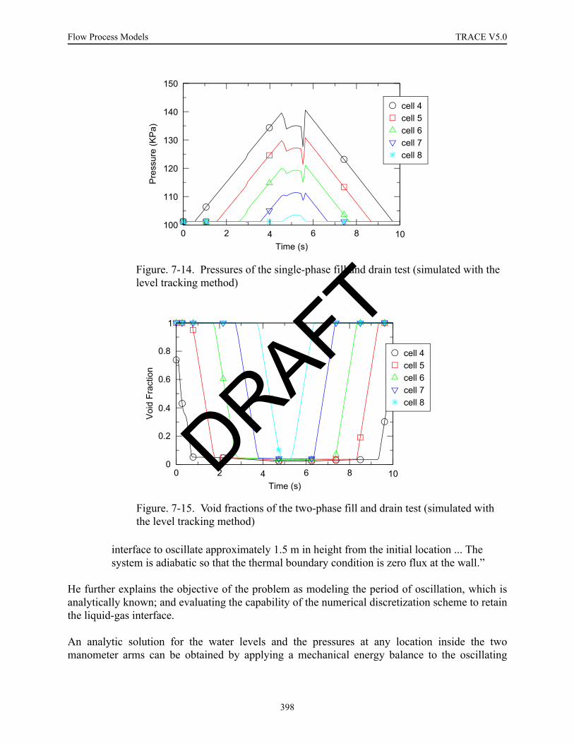
Flow Process Models TRACE V5.0
interface to oscillate approximately 1.5 m in height from the initial location ... The system is adiabatic so that the thermal boundary condition is zero flux at the wall.”
He further explains the objective of the problem as modeling the period of oscillation, which isanalytically known; and evaluating the capability of the numerical discretization scheme to retainthe liquid-gas interface.
An analytic solution for the water levels and the pressures at any location inside the twomanometer arms can be obtained by applying a mechanical energy balance to the oscillating
Figure. 7-14. Pressures of the single-phase fill and drain test (simulated with the level tracking method)
Figure. 7-15. Void fractions of the two-phase fill and drain test (simulated with the level tracking method)
0 2 4 6 8 10Time (s)
100
110
120
130
140
150
Pre
ssur
e (K
Pa)
cell 4cell 5cell 6cell 7cell 8
0 2 4 6 8 10Time (s)
0
0.2
0.4
0.6
0.8
1
Voi
d Fr
actio
n
cell 4cell 5cell 6cell 7cell 8
DRAFT
398

TRACE V5.0 Flow Process Models FOOBAR1234FOOBAR1234FOOBAR1234FOOBAR1234FOOBAR1234FOOBAR1234
Flow Process
Models
water slug. In the absence of any losses, the mechanical energy balance dictates that the gain oftotal potential energy is always equal to the loss of total kinetic energy and vice versa.
Figure. 7-16. Pressures of the two-phase fill and drain test (simulated with the level tracking method)
Figure. 7-17. Schematic of the oscillating manometer test
0 2 4 6 8 10Time (s)
100
110
120
130
140
150
Pre
ssur
e (K
Pa)
cell 4cell 5cell 6cell 7cell 8
1
2
3
4
5
6
7
8
9
10
L/2=
5m
+1.5m
-1.5m
h(t)
t0DRAFT
399

Flow Process Models TRACE V5.0
(7-94)
Defining the length of the oscillating slug , and the cross sectional area of the manometer arm, the distance between the water level at any time to its initial position with , and the
velocity of the oscillating slug with , the change of kinetic energy and potential energy withrespect to time can be expressed as follows:
(7-95)
(7-96)
. (7-97)
Equation (7-97) can be solved for the location of the manometer water level as function of time,i.e. , with the initial conditions that specify the initial position of the oscillating slug and itsvelocity:
, (7-98)
The solution of Eq. (7-97) yields the distance between the surface of the oscillating water levelsand their starting location inside the left and right manometer arms:
and (7-99)
where the period of the oscillating manometer is found to be
. (7-100)
Once the location of the oscillating manometer water level is known as a function of time,pressures at any point along the manometer arm can be determined from a simple force balancebetween the point of interest and the surface of the oscillating water level. The force balanceshould include the terms due to fluid acceleration and gravity:
tddK
tddΦ+ 0=
LS H t( )
V t( )
tdd 1
2---ρV2 t( )SL
⎝ ⎠⎜ ⎟⎛ ⎞
tdd ρgSz zd
0
H t( )
∫ ρgSz zdH t( )–
0
∫+⎝ ⎠⎜ ⎟⎜ ⎟⎛ ⎞
+ 0=
LV t( )td
d V t( ) 2gH t( )td
d H t( )+ 0=
t
2
dd H t( )
2gL------
⎝ ⎠⎜ ⎟⎛ ⎞
H t( )+ 0=
H t( )
H t( ) 0=td
dH
t 0=
V0=
HL t( )V0T2π
----------- 2πtT
---------⎝ ⎠⎜ ⎟⎛ ⎞
sin= HR t( ) HL t( )–=
T 2π L2g------=
DRAFT
400
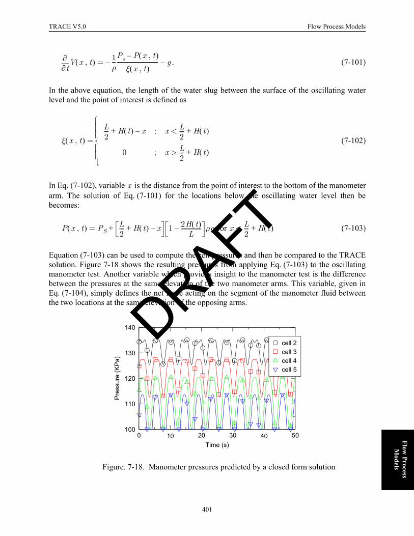
TRACE V5.0 Flow Process Models FOOBAR1234FOOBAR1234FOOBAR1234FOOBAR1234FOOBAR1234FOOBAR1234
Flow Process
Models
. (7-101)
In the above equation, the length of the water slug between the surface of the oscillating waterlevel and the point of interest is defined as
(7-102)
In Eq. (7-102), variable is the distance from the point of interest to the bottom of the manometerarm. The solution of Eq. (7-101) for the locations below the oscillating water level then bebecomes:
for (7-103)
Equation (7-103) can be used to compute the cell pressures and then be compared to the TRACEsolution. Figure 7-18 shows the resulting pressures from applying Eq. (7-103) to the oscillatingmanometer test. Another variable which provides insight to the manometer test is the differencebetween the pressures at the same elevation of the two manometer arms. This variable, given inEq. (7-104), simply defines the net force acting on the segment of the manometer fluid betweenthe two locations at the same elevation of the opposing arms.
Figure. 7-18. Manometer pressures predicted by a closed form solution
t∂∂ V x t,( ) 1
ρ---Ps P x t,( )–
ξ x t,( )------------------------------– g–=
ξ x t,( )
L2--- H t( ) x–+ ; x L
2--- H t( )+<
0 ; x L2--- H t( )+>
⎩⎪⎪⎨⎪⎪⎧
=
x
P x t,( ) PSL2--- H t( ) x–+ 1 2H t( )
L---------------– ρg+= x L
2--- H t( )+<
0 10 20 30 40 50Time (s)
100
110
120
130
140
Pre
ssur
e (K
Pa)
cell 2cell 3cell 4cell 5
DRAFT
401
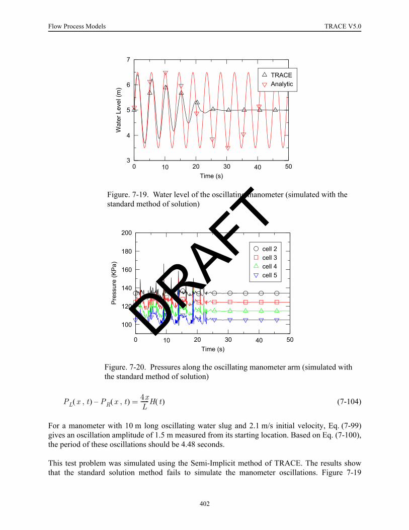
Flow Process Models TRACE V5.0
(7-104)
For a manometer with 10 m long oscillating water slug and 2.1 m/s initial velocity, Eq. (7-99)gives an oscillation amplitude of 1.5 m measured from its starting location. Based on Eq. (7-100),the period of these oscillations should be 4.48 seconds.
This test problem was simulated using the Semi-Implicit method of TRACE. The results showthat the standard solution method fails to simulate the manometer oscillations. Figure 7-19
Figure. 7-19. Water level of the oscillating manometer (simulated with the standard method of solution)
Figure. 7-20. Pressures along the oscillating manometer arm (simulated with the standard method of solution)
0 10 20 30 40 50Time (s)
3
4
5
6
7
Wat
er L
evel
(m)
TRACEAnalytic
0 10 20 30 40 50Time (s)
100
120
140
160
180
200
Pre
ssur
e (K
Pa)
cell 2cell 3cell 4cell 5
PL x t,( ) PR x t,( )– 4xL------H t( )=
DRAFT
402

TRACE V5.0 Flow Process Models FOOBAR1234FOOBAR1234FOOBAR1234FOOBAR1234FOOBAR1234FOOBAR1234
Flow Process
Models
compares the collapsed water level predicted by TRACE to the oscillating water level predictedby Eq. (7-99). A comparison of the pressures along the manometer arm predicted by TRACE andEq. (7-103) (see Figure 7-20) reveals that the standard solution method of TRACE dissipates thekinetic energy of the oscillating fluid very quickly. This conclusion is more obvious when the netforce acting on a given segment of the oscillating fluid described by Eq. (7-104) is considered.Figure 7-21 compares the net force acting on a segment of oscillating fluid contained between2.5 m elevation in one manometer arm to 2.5 m elevation in the opposing arm. This comparisonconcurs that the solution with the upwind donor method quickly dissipates the kinetic energy ofthe oscillating fluid. It is therefore concluded that the standard solution method of TRACE, i.e.Semi-Implicit method, fails to simulate the oscillating manometer test.
The oscillating manometer test simulated with level tracking. The solution method with the leveltracking failed to simulate this test prior to the additional considerations made for the liquid-gasinterface crossing the cell boundaries.
The leading cause of this failure to simulate the oscillating manometer was the pressure spikescaused by the interface crossing cell boundaries. Figure 7-23 shows none of these pressure spikes.Thus, the water level of the manometer arm oscillates without any sign of decay as expected inFigure 7-22. Further, the simulated cell pressures below the oscillating water level in Figure 7-18compare almost perfectly with the pressures predicted analytically in Figure 7-18. These resultsfor the oscillating manometer test are as close as a dicrete solution can be to the analyticalsolution for the oscillating manometer, which is a point that demonstrates the success of theapproach outlined in this section to propagate interfaces across cell boundaries.
Figure. 7-21. The net force on the fluid segment below 2.5 m elevation of the manometer arms (simulated with the standard method of solution)
0 10 20 30 40 50Time (s)
-30
-20
-10
0
10
20
30
Diff
eren
tial P
ress
ure
(Kpa
) TRACEAnalytic
DRAFT
403
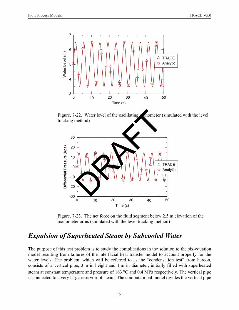
Flow Process Models TRACE V5.0
Expulsion of Superheated Steam by Subcooled Water
The purpose of this test problem is to study the complications in the solution to the six-equationmodel resulting from failures of the interfacial heat transfer model to account properly for thewater levels. The problem, which will be referred to as the “condensation test” from hereon,consists of a vertical pipe, 3 m in height and 1 m in diameter, initially filled with superheatedsteam at constant temperature and pressure of 163 oC and 0.4 MPa respectively. The vertical pipeis connected to a very large reservoir of steam. The computational model divides the vertical pipe
Figure. 7-22. Water level of the oscillating manometer (simulated with the level tracking method)
Figure. 7-23. The net force on the fluid segment below 2.5 m elevation of the manometer arms (simulated with the level tracking method)
0 10 20 30 40 50Time (s)
3
4
5
6
7
Wat
er L
evel
(m)
TRACEAnalytic
0 10 20 30 40 50Time (s)
-30
-20
-10
0
10
20
30
Diff
eren
tial P
ress
ure
(Kpa
)
TRACEAnalytic
DRAFT
404

TRACE V5.0 Flow Process Models FOOBAR1234FOOBAR1234FOOBAR1234FOOBAR1234FOOBAR1234FOOBAR1234
Flow Process
Models
into ten equal computational volumes. A schematic diagram of the test problem is shown inFigure 7-25. Also shown in Figure 7-25 is the three-dimensional version of the same test thatdivides the vertical pipe into 80 equal computational volumes. During the test, liquid watersubcooled at 50 oC is injected with 0.5 m/s velocity at the bottom inlet of the pipe until it fills thepipe completely. The recommended maximum timestep size for the simulation of this test is 0.05seconds.
This test problem was designed to measure the ability of a solution method to cope with thedifficulties which arise from inaccurate modelling of the computational volumes as they are filledby the rising liquid front. Predicting the interfacial heat transfer rate in these volumes, and thereof,the condensation of superheated steam in contact with the very subcooled water is very critical tothe successful simulation of this test. There is also an added complexity as a saturated layer ofliquid builds up in the tail of the rising front that should continuously decrease the condensationrate. A solution method without proper care for these details is expected to suffer severely as acell becomes “packed” with liquid water when the method fails to turn off the condensationbehind the rising liquid front.
The standard solution method of TRACE displays the expected difficulties due to water packingand inaccurate modeling of the condensation at the rising liquid front. Figure 7-26 shows thepressures at each computation volume along the pipe as the subcooled water is injected. Thepresence of the water packing phenomenon is apparent in this figure. The magnitude of theresulting compression waves from the “numerical” water hammer reaches to 2.5 MPa renderingthe TRACE solution unusable. Before drawing a conclusion on the performance of TRACE, thewater packing option, an optional method that overcomes the fluid packing problem bydampening the pressure field, must be engaged in the simulation of the condensation test. Figure7-27 shows the pressures along the test pipe recomputed by TRACE with the water packingoption.
Figure. 7-24. Pressures along the oscillating manometer arm (simulated with the level tracking method)
0 10 20 30 40 50Time (s)
100
110
120
130
140
Pre
ssur
e (K
Pa) cell 2
cell 3cell 4cell 5
DRAFT
405

Flow Process Models TRACE V5.0
Although the amplitude of pressure spikes are several times smaller, their mere presence issufficient to prove that the standard method of solution even with the help from a special methodis still unable to handle properly the steam condensation at the rising liquid front.
Another variable of equal interest is the liquid temperature along the pipe which is expected toindicate the build up of a saturated liquid layer behind the rising front. Figure 7-28 shows that theliquid temperatures follow rather closely the sub-cooled temperature with occasional jumps to thesaturation temperature in the vicinity of the rising front. As sub-cooled water is injected at thebottom, superheated steam is withdrawn into the pipe at the top replenishing the steam beingcondensed at such extreme rates. Normally, the direction of steam flow should be an outcome of abalance between the volume rate at which liquid displaces steam and the volume rate at whichsteam is being condensed at the front. However, the compression waves induced by the fluidpacking dominates the TRACE solution causing high bursts of steam flowing out of the test pipeas seen in Figure 7-29.
Figure. 7-25. Schematic of the 1D and 3D condensation tests
L=3m
Subcooled water injectionT = 50.0oCVin = 0.5m/s
Superheated steamp = 0.4MPaT = 163.0C
1
2
3
4
5
6
7
8
9
10
32
41 5
6
7
8
1
2
3
4
5
6
7
8
9
10
DRAFT
406
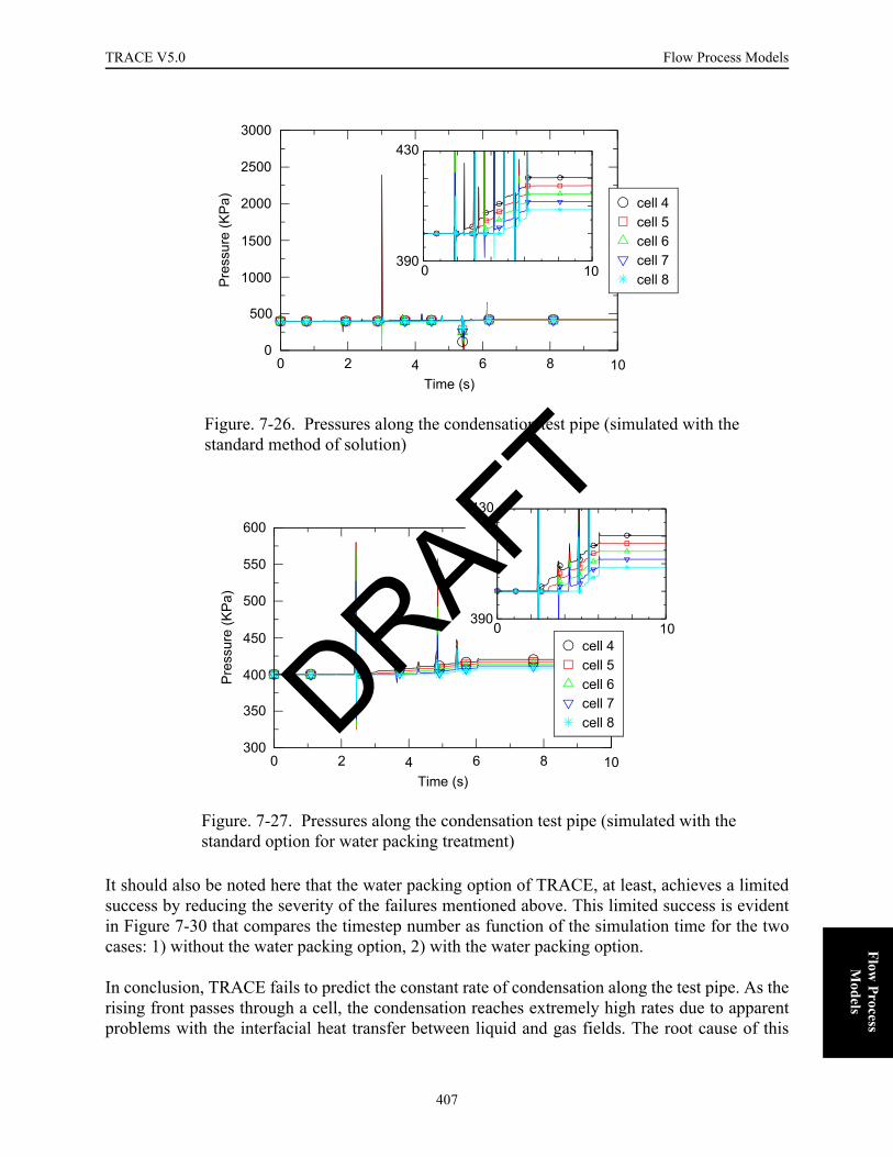
TRACE V5.0 Flow Process Models FOOBAR1234FOOBAR1234FOOBAR1234FOOBAR1234FOOBAR1234FOOBAR1234
Flow Process
Models
It should also be noted here that the water packing option of TRACE, at least, achieves a limitedsuccess by reducing the severity of the failures mentioned above. This limited success is evidentin Figure 7-30 that compares the timestep number as function of the simulation time for the twocases: 1) without the water packing option, 2) with the water packing option.
In conclusion, TRACE fails to predict the constant rate of condensation along the test pipe. As therising front passes through a cell, the condensation reaches extremely high rates due to apparentproblems with the interfacial heat transfer between liquid and gas fields. The root cause of this
Figure. 7-26. Pressures along the condensation test pipe (simulated with the standard method of solution)
Figure. 7-27. Pressures along the condensation test pipe (simulated with the standard option for water packing treatment)
0 2 4 6 8 10Time (s)
0
500
1000
1500
2000
2500
3000
Pre
ssur
e (K
Pa) cell 4
cell 5cell 6cell 7cell 80 10
390
430
0 2 4 6 8 10Time (s)
300
350
400
450
500
550
600
Pres
sure
(KPa
)
0 10390
430
cell 4cell 5cell 6cell 7cell 8DRAFT
407
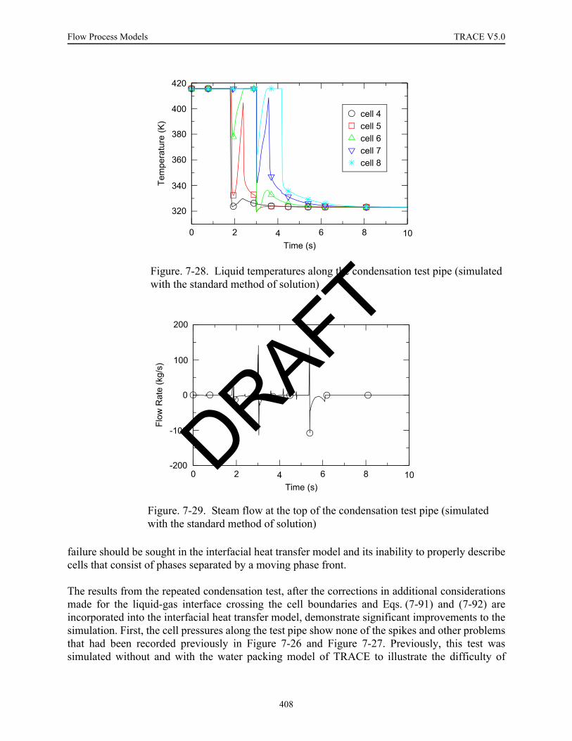
Flow Process Models TRACE V5.0
failure should be sought in the interfacial heat transfer model and its inability to properly describecells that consist of phases separated by a moving phase front.
The results from the repeated condensation test, after the corrections in additional considerationsmade for the liquid-gas interface crossing the cell boundaries and Eqs. (7-91) and (7-92) areincorporated into the interfacial heat transfer model, demonstrate significant improvements to thesimulation. First, the cell pressures along the test pipe show none of the spikes and other problemsthat had been recorded previously in Figure 7-26 and Figure 7-27. Previously, this test wassimulated without and with the water packing model of TRACE to illustrate the difficulty of
Figure. 7-28. Liquid temperatures along the condensation test pipe (simulated with the standard method of solution)
Figure. 7-29. Steam flow at the top of the condensation test pipe (simulated with the standard method of solution)
0 2 4 6 8 10Time (s)
320
340
360
380
400
420
Tem
pera
ture
(K)
cell 4cell 5cell 6cell 7cell 8
0 2 4 6 8 10Time (s)
-200
-100
0
100
200
Flow
Rat
e (k
g/s)
DRAFT
408

TRACE V5.0 Flow Process Models FOOBAR1234FOOBAR1234FOOBAR1234FOOBAR1234FOOBAR1234FOOBAR1234
Flow Process
Models
simulating this test. A comparison of the required number of time steps as a function of thesimulation time from the two simulations in Figure 7-30 had revealed a limited success with thewater packing. When the water packing model of TRACE was engaged, the total number of timesteps was reduced from 3000 to just below 1000. The adjustments made to the IHT model reducesthe total number of time steps to 500. Figure 7-32 compares the number of time steps required tosimulate the condenstation test with the standard solution, with the solution aided by the waterpacking model, and with the solution improved by the level tracking method. It is clear fromFigure 7-32 that no additional time steps are needed as the moving crosses the cell boundarieswhen the level tracking method is engaged. The timestep number as function of simulation time
Figure. 7-30. Comparison of total time step numbers of condenstation test simulations (with and without the option for water packing treatment)
Figure. 7-31. Pressures along the condensation test pipe (simulated with the level tracking method)
0 2 4 6 8 10Time (s)
0
500
1000
1500
2000
2500
3000
Tim
e S
tep
Num
ber
Without PackingWith Packing
0 2 4 6 8 10Time (s)
390
400
410
420
430
Pre
ssur
e (K
Pa)
cell 4cell 5cell 6cell 7cell 8
DRAFT
409

Flow Process Models TRACE V5.0
from the water packing exercise is compared to the repeated simulation following the changes toIHT in Figure 7-32 where the total number of timesteps is reduced to 585. The figure also showsthat the solution spends no extra timestep as the moving water level fills up the cells with liquidwater. This improvement is expected since the water packing model is a remedy for troubles aftera cell is already “packed” while the level tracking method predicts the “packing” before ithappens and adjusts the initial conditions of a time step to avoid the “packing.”
As discussed previously, the superheated steam is withdrawn into the test pipe at the top toreplenish the steam being condensed at it meets the subcooled water at the interface. Previously,large rates of steam flow were recorded in Figure 7-29 because of erroneous condensation takingplace inside the test pipe. Figure 7-33 shows that the steam flow rate is much smaller and orderlywhen the solution is improved by the level tracking method. However, an irregular change incondensation is observed as the water level traverses the “inlet” and “exit” computationalvolumes of the test pipe. This inaccurate behavior is due to an inconsistent treatment of the endcells of one-dimensional flow segments defined within TRACE, and not due to the level trackingmethod.
One of difficulties stated for this exercise was the added complexity due to the build-up of asaturated layer of liquid at the tail of the moving water level. As this layer builds up, it shouldcontinuously decrease the rate at which the steam condenses at the surface. While there is noassurance yet for the accuracy of TRACE’s ability to predict the condensation at the interface, aslight and gradual decrease in the condensation is observed as the water level traverses the“interior” cells of the test pipe. This observation is also enforced by the liquid temperatures shownin is seen in the simulation was due to an error in IHT coefficients for limiting void fractions, theliquid temperatures in Figure 7-34 that shows the build up of a warmer liquid layer. While acomparison of the liquid temperatures in Figure 7-34 to the temperatures previously recorded inFigure 7-28 leaves no doubt about the improvements to TRACE realized by the level tracking
Figure. 7-32. Comparison of total time step numbers of the condenstation test simulations
0 2 4 6 8 10Time (s)
0
500
1000
1500
2000
2500
3000
Tim
e St
ep N
umbe
r Without PackingWith PackingWith Tracking
DRAFT
410

TRACE V5.0 Flow Process Models FOOBAR1234FOOBAR1234FOOBAR1234FOOBAR1234FOOBAR1234FOOBAR1234
Flow Process
Models
method, it is extremely important to assess TRACE’s ability to predict the interfacial heat transferrate at the surface of liquid-gas interfaces by simulating an experiment with available data. Thedesired capability for TRACE is to predict the “correct” rate of condensation and the build-up ofwarmer liquid layer only due to the IHT at the surface of the water level.
Figure. 7-33. Steam flow at the top of the condensation test pipe (simulated with the level tracking method)
Figure. 7-34. Liquid temperatures along the condensation test pipe (simulated with the level tracking method)
0 2 4 6 8 10Time (s)
-2
-1.5
-1
-0.5
0
0.5
Flow
Rat
e (k
g/s)
0 2 4 6 8 10Time (s)
320
340
360
380
400
420
Tem
pera
ture
(K)
cell 4cell 5cell 6cell 7cell 8
DRAFT
411

Flow Process Models TRACE V5.0
Summary of the Simulations
All of the test problems discussed in this chapter are designed to measure the performance of thesemi-implicit method of solution to the six-equation model in the presence of moving waterlevels. However, it should also be emphasized that these problems are designed to reveal thedifficulties of a method and magnify them as much as possible, if there is any, so that thesedifficulties can be identified and studied further.
The results of the numerical experiments presented in this chapter can be summarized as follows:
1) All of the tests reveal that the solution method in TRACE fails to predict accurately the acceleration of liquid and gas fields in vertical paths when both fields are separated by a stratified liquid-gas interface. This failure is evident from the figures that show the transient behavior of fluid pressure in all tests.
2) The solution methods like the semi-implicit method, which are equipped with the stan-dard upstream donor method in general, are unable to retain the liquid-gas interface. The figures that show the void fraction along the test pipes suggest that numerical dif-fusion of fluid mass is very high in the presence of stratified liquid-gas interface. Unlike the diffusion due to the discrete nature of the solution, the root cause of this failure is hidden behind the inability of the upstream donor method to recognize that a computational volume consists of two sub-volumes separated by a liquid-gas inter-face.
3) The mixture of steam and water poses added complexities due to the inability of the interfacial heat transfer model to distinguish the two sub-volumes, which are topologi-cally different, separated by the liquid-gas interface. As the interfacial heat transfer model determines the heat transfer coefficients based on volume average void fraction, the interfacial heat transfer between the two fields is over or under predicted for the computational volume that consists of the liquid-gas interface.
4) The current measures built into the solution method, e.g. the water packing option, have limited success in mitigating the consequences of numerical water hammer when the sudden condensation is initiated by moving liquid-gas interfaces.
Offtake ModelThe TRACE TEE-component offtake model is designed specifically to handle the case of fluidflow through a small break that is made in a larger pipe containing horizontal stratified flow (Ref.7-12). One example of a transient that is particularly well-suited for use with the offtake model isa LOCA, in which a small break occurs in one of the large-diameter horizontal pipes of the reactorinlet or outlet legs. During this transient, horizontal stratified flow may occur and the flow qualitydischarged at the break will depend on whether the break is above or below the liquid level. Toaccurately follow the progression of the transient, it is essential that the offtake flow be predictedcorrectly.
DRAFT
412

TRACE V5.0 Flow Process Models FOOBAR1234FOOBAR1234FOOBAR1234FOOBAR1234FOOBAR1234FOOBAR1234
Flow Process
Models
The TRACE TEE-component offtake model predicts the offtake flow quality that exits the breakbased on conditions in the main pipe in a manner similar to that developed for use in theRELAP5/MOD2 code (Ref. 7-13). When the entrance plane to the break is submerged, the offtakeflow consists mostly of liquid with possibly an entrained gas component. When the entrance planeis above the liquid level, the offtake flow is mostly gas with possibly an entrained liquidcomponent.
The model is implemented as an option that the user may activate via input. To use the model forits intended purpose, the following three assumptions on the geometry of the problem areenforced in the code:
1) The side tube of the TEE is required to be either top, bottom, or centrally located off the main tube.
2) The angle from the low-numbered side of the main tube to the side tube must be 90°.
3) The main-tube-junction cell must be horizontal.
If these three conditions are not met by the input deck TEE geometry, the problem terminates inthe initialization stage with a fatal error concerning inappropriate offtake geometry.
Several studies have been performed to investigate the discharge characteristics of a small breaklocated on a horizontal pipe containing stratified flow. In these studies, the offtake was either top,bottom, or centrally oriented from the main tube as shown in Figure 7-35. The followingdiscussion describes each of these three offtake geometries and the flow correlations developedfor Reference 7-13. The TRACE computational sequence for the offtake model and a moredetailed description of the original experimental work may be found in Appendix D andReferences 7-14 to 7-17.
In each of the three offtake configurations of Figure 7-35, a critical height at which gas or liquidentrainment begins, , may be calculated using major-phase conditions at the entrance plane,such that:
(7-105)
where = a constant determined from data, = major-phase mass-flow rate,
= gravitational constant, = major-phase density, and = phasic densitydifference. For an upward offtake or for a side-oriented offtake with a liquid level below theofftake center, the major phase comprises the gas component. For a downward offtake or for aside-oriented offtake with a liquid level above the offtake center, the liquid component constitutesthe major phase. The values of the constant recommended for use by Reference 7-12 are
summarized in Table 7-1. This formulation for can be derived theoretically for each of thethree offtake geometries by considering the force exerted on the liquid particles by the
hb
hbC1Wk
0.4
gρk∆ρ( )0.2----------------------------=
C1 Wk
g ρk ρ∆ ρl ρg–=
C1
hb
DRAFT
413

Flow Process Models TRACE V5.0
accelerating gas flow for liquid entrainment in upward or side-oriented offtakes and byconsidering surface instability effects for gas entrainment in downward offtakes (Refs. 7-13, 7-16and 7-17). An actual characteristic height, , measured as the distance from the offtake entranceplane to the liquid level, may be determined for each of the three offtake geometries as shown inFigure 7-36.
The nondimensional height ratio, , then may be represented as
(7-106)
Figure. 7-35. Possible offtake configurations
Table 7-1. Critical Height Correlation Constant
Offtake Geometry Correlation Constant, C1
Upward 1.67
Downward 1.50
Side (gas entrain.) 0.75
Side (liquid entrain.) 0.69
h
R
R hhb-----=
DRAFT
414
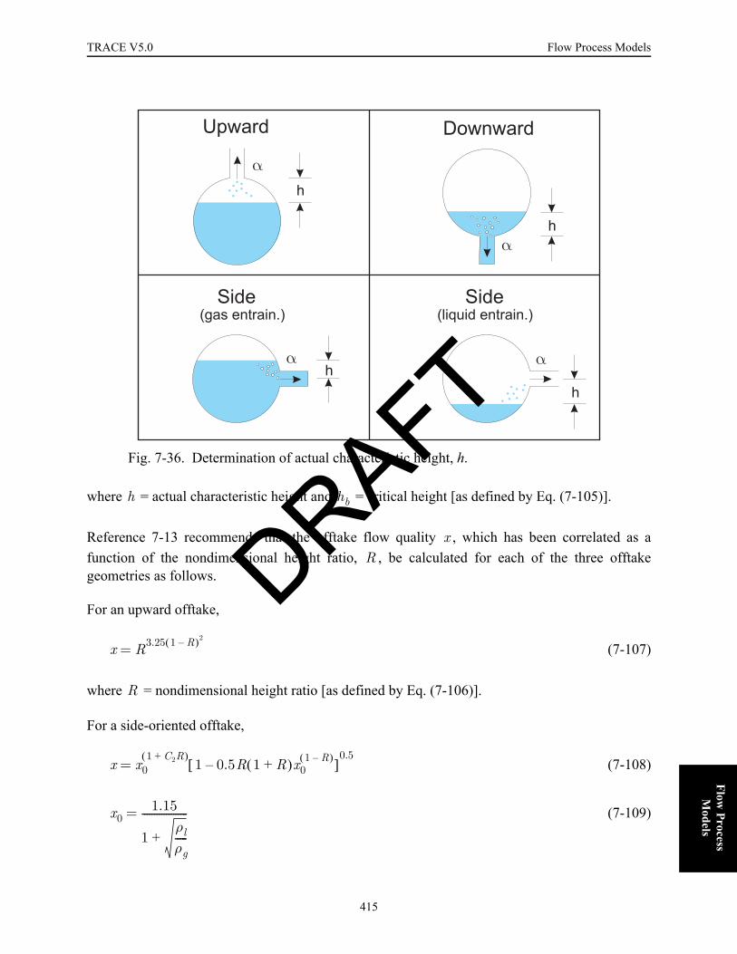
TRACE V5.0 Flow Process Models FOOBAR1234FOOBAR1234FOOBAR1234FOOBAR1234FOOBAR1234FOOBAR1234
Flow Process
Models
where = actual characteristic height and = critical height [as defined by Eq. (7-105)].
Reference 7-13 recommends that the offtake flow quality , which has been correlated as afunction of the nondimensional height ratio, , be calculated for each of the three offtakegeometries as follows.
For an upward offtake,
(7-107)
where = nondimensional height ratio [as defined by Eq. (7-106)].
For a side-oriented offtake,
(7-108)
(7-109)
Fig. 7-36. Determination of actual characteristic height, h.
h
h
h
h
Upward Downward
Side Side(gas entrain.) (liquid entrain.)
h hb
xR
x R3.25 1 R–( )2
=
R
x x01 C2R+( )
1 0.5R 1 R+( )x01 R–( )–[ ]
0.5=
x01.15
1ρlρg-----+
-------------------=
DRAFT
415
Flow Process Models TRACE V5.0
= nondimensional height ratio [as defined by Eq. (7-106)], = liquid-phase density at the
entrance plane, = gas-phase density at the entrance plane, and = 1.09 for gas entrainmentor 1.00 for liquid entrainment.
For a downward offtake,
(7-110)
where is given by Eq. (7-109), = nondimensional height ratio [as defined by Eq. (7-106)],
= liquid-phase density at the entrance plane, and = gas-phase density at the entrance plane.
From the prediction of the offtake quality and knowledge of the phasic velocities and densities atthe break, TRACE finally determines the offtake void fraction.
In conclusion, summarizing, the TRACE TEE-component offtake model predicts the flowdischarged from a small break that is located in a large pipe containing horizontal stratified flow.The current model is able to accommodate three different offtake geometries: upward offtake,side-oriented offtake, and downward offtake. TRACE calculates an offtake void fraction fromflow correlations for the particular offtake geometry being modeled. As explained in more detailin Appendix D, a first prediction of the offtake void fraction is then sent through oneinterpolation based on the liquid level, one weighting based on the degree of horizontalstratification and one limit based on the maximum allowable entrainment volume to arrive at thefinal offtake void fraction.
Form Loss ModelsThere are four contributions to the pressure gradient for steady-state single phase pipe flow: walldrag, gravity head, recoverable flow-area change loss/gain, and irrecoverable loss. The purposeof this section is to document how TRACE deals with the recoverable and irrecoverablecontributions to the overall pressure gradient.
The recoverable flow area change loss/gain comes from the change in the momentum flux term inthe TRACE momentum equations. Consider the single-phase steady-state momentum equationwith gravity and wall shear neglected:
. (7-111)
For a pipe noded as in Figure 7-37, integration of Eq. (7-111) with the assumptions of steady stateand of constant density from point to point yields a Bernoulli-type equation for thepressure change from point to point as follows:
R ρl
ρg C2
x x02.5R 1 0.5R 1 R+( )x0
1 R–( )–[ ]0.5
=
xo R
ρl ρg
1ρ--- ∂P
∂x------- V ∂V
∂x--------+ 0=·
j j 1+j j 1+
DRAFT
416

TRACE V5.0 Flow Process Models FOOBAR1234FOOBAR1234FOOBAR1234FOOBAR1234FOOBAR1234FOOBAR1234
Flow Process
Models
(7-112)
In terms of the pressure drop from cell center to cell center , Eq. (7-112) becomes
. (7-113)
Assuming constant volumetric flow from to , then Eq. (7-113) can be written as:
(7-114)
From Eq. (7-114), it should be obvious that a sudden contraction (see Figure 7-38), where, will result in a positive pressure drop, while a sudden expansion (see Figure 7-39),
where , will result in a negative pressure drop. It should also be obvious that thepressure loss for a sudden contraction followed by a sudden expansion with the same area ratiowill result in complete recovery of the sudden contraction pressure loss. As a result, the pressuredifference due to the change in momentum flux is typically referred to as the recoverable flowarea change pressure loss/gain.
Note – The TRACE one-dimensional staggered difference scheme involves pressures at cell centers and velocities at cell edges. In addition, the backward differencing for the change in momentum flux has been found to be stable and robust, but does not yield a Bernoulli-like solution for single phase incompressible flow. Therefore, an area ratio model — described in Chapter 1 — was developed to ensure that the stable and robust differencing in TRACE also accurately conserves momentum flux.
Figure. 7-37. 1D TRACE noding.
j – 1 j j + 1 j + 2
j – 1/2j – 3/2 j + 1/2 j + 3/2 j + 5/2
Pj 1+ Pj– ρVj
2
2------
Vj 1+2
2-------------–
⎝ ⎠⎜ ⎟⎛ ⎞
=
j j 1+
∆Pj j 1+→
Pj 1+ Pj–( )–= ρVj 1+
2
2-------------
Vj2
2------–
⎝ ⎠⎜ ⎟⎛ ⎞
=
j j 1+
∆Pj j 1+→
ρVj
2
2------
AjAj 1+-------------
⎝ ⎠⎜ ⎟⎛ ⎞
2
1–=
Aj Aj 1+<Aj 1+ Aj<
DRAFT
417

Flow Process Models TRACE V5.0
Figure. 7-38. TRACE noding for abrupt contraction if and for abrupt expansion if .
Figure. 7-39. TRACE noding for abrupt expansion if and for abrupt contraction if .
Figure. 7-40. TRACE noding for sharp-edged, thin-plate orifice.
j – 1 j j + 1 j + 2
j – 1/2j – 3/2 j + 1/2 j + 3/2 j + 5/2
Positive Flow
Vj 1 2⁄+ 0>Vj 1 2⁄+ 0<
j – 1 j j + 1 j + 2
j – 1/2j – 3/2 j + 1/2 j + 3/2 j + 5/2
Positive Flow
Vj 1 2⁄+ 0>Vj 1 2⁄+ 0<
j – 1 j j + 1 j + 2
j – 1/2j – 3/2 j + 1/2 j + 3/2 j + 5/2
Positive Flow
DRAFT
418

TRACE V5.0 Flow Process Models FOOBAR1234FOOBAR1234FOOBAR1234FOOBAR1234FOOBAR1234FOOBAR1234
Flow Process
Models
Irrecoverable pressure losses occur at area changes, pipe bends, flow through orifice, flowthrough tee or manifold, etc. These irrecoverable pressure losses are associated withirrecoverable energy loss from the system typically associated with the creation of turbulence andthe deviation of the flow from smooth straight stream lines. The modeling equation in TRACEfor this irrecoverable pressure loss is based on a form loss factor of the form
(7-115)
So let’s put this together with what we know already about the reversible losses. Consider thefollowing three situations. If no area change occurs between points and , the velocity of theflow does not change, and Eq. (7-113) predicts
(7-116)
as expected. If a smooth area change occurs between sections and , then the irreversiblelosses may be small, and Eq. (7-113) yields an approximation to the pressure drop from point to
. If the area change between cells and is abrupt, however, the irreversible lossescannot be ignored, and it is standard practice to add a form-loss factor like that shown inEq. (7-115) to Eq. (7-113) to account for the additional irrecoverable pressure loss caused by thearea change in question. This yields a general equation for the pressure drop between sections and when an abrupt area change is present, such that
(7-117)
where is the velocity at the cross section where the area change occurs. Once the loss
coefficient for the specific area change in question has been determined, either theoretically orexperimentally, the pressure drop at the abrupt area change can be calculated using Eq. (7-117)above.
The big question, of course, is "where do the K-factors come from?" TRACE provides the abilityto account for irrecoverable losses via user input by supplying a form loss factor at any 1D or 3Dcell edge. Situations that might require the need to specify a non-zero K-factor include flowthrough abrupt expansions or contractions, flow across a thin-plate orifice, flow around a bend,flow streams that merge or split, flow across obstructions, etc (really, any complex flow topologythat leads to separation of the flow from the wall). Normally, it is incumbent upon the user toconsult a body of knowledge like Reference 7-18 or 7-19 to determine the appropriate K-factorfor the situation at hand.
∆Pirreversible ρKV2
2------∼
j j 1+
∆Pj j 1+→
0=
j j 1+j
j 1+ j j 1+
jj 1+
∆Pj j 1+→
Pj 1+ Pj–( )–= ρVj 1+
2
2-------------
Vj2
2------–
⎝ ⎠⎜ ⎟⎛ ⎞
ρKV
j 1 2⁄+2
2------------------+=
Vj 1 2⁄+
K
DRAFT
419

Flow Process Models TRACE V5.0
For the case of abrupt area expansions and contractions in 1D and 3D flow channels, TRACE isable to determine, on its own, the appropriate K-factor, provided you have engaged the propermodeling flag (see the description of the NFF flag in the TRACE User’s Guide). In suchinstances, TRACE will calculate a form-loss coefficient based on the user-input cell-edge flow
area, the volume-averaged mesh-cell flow area ( ), and the direction of the fluidvelocity. TRACE then adds this additional form-loss term to the momentum equation to accountfor the irrecoverable losses caused by the abrupt area change. These models are described insubsections below.
Note – In order to support old TRAC-P input models, TRACE retains the capability for the user to provide additive FRIC values rather than form loss factors to simulate irrecoverable losses. The relationship between form loss factors and FRIC input values is given by , where
is the cell-center to cell-center distance and is the user-supplied hydraulic diameter for the cell edge for which the FRIC value has been input. In general, you should use K-factors, since formulas and data for form loss factors are available, while FRIC values require additional computations for input preparation. In addition, any changes in noding around a user-input FRIC requires that the user re-calculate the input for FRIC
The flow loss of a thin-plate orifice that is modeled at a mesh-cell interface is associated with anabrupt flow-area change. This flow loss is also discussed below, but it is not added by TRACEautomatically as an additional loss because . Such losses that are modeled at interfaces need to bedefined by the user through additive form-loss-coefficient input data.
In a related way, the existence of a thin-plate orifice creates an abrupt flow-area change and alsoresults in irrecoverable pressure losses. While methods do exist to determine the appropriate losscoefficient analytically, in practice, we have found this impossible to implement as an automaticoption because there is no unique criteria for detecting such a flow topology. It is possible tocreate input models that have cell-edge flow areas that are less than both of the bounding mesh-cell flow areas, even though in reality there is no thin-plate orifice. Therefore, if a thin-plateorifice exists, you must supply your own user-defined K-factors to account for the irreversiblelosses; there is no internal calculation for such a loss that can be selected via the input. Arecommendation for user determination of an appropriate loss coefficient is given in a subsectionbelow.
Before proceeding, it is worth noting that there is no input option to select automatic internalcalculation of losses from abrupt expansions or contractions at the three interfaces of the TEEjoining cell. Also, the flow-area ratios logic for reversible losses (as documented in Chapter 1) isnot activated at the three interfaces of the TEE joining cell. As such, you must account for anyadditional losses that result from flow merging, splitting, or abrupt area changes with appropriateuse of the form-loss input array data that specifies K-factors at 1D mesh-cell interfaces. Reference7-201 is a source of such data. The current TEE-component momentum-source-term logic is
1. You are cautioned to note that the correlations for TEE losses in this document include velocities based on experiments that have equal flow areas in all three TEE flow channels.
Aj volj ∆xj⁄=
K FRIC L·( ) D⁄=L D
DRAFT
420

TRACE V5.0 Flow Process Models FOOBAR1234FOOBAR1234FOOBAR1234FOOBAR1234FOOBAR1234FOOBAR1234
Flow Process
Models
discussed in Chapter 1. We note here that while this model exhibits numerical stability, it doesnot give perfect predictions of losses at TEE internal junctions. Usually, the current model willunderpredict TEE losses, although in some situations the losses will be overpredicted.
Abrupt Expansion
To determine the loss coefficient for an abrupt expansion, consider the expansion of Figure 7-41.If the pipes run full and the flow is assumed steady, two simplifying assumptions may be madethat allow the pressure change across the expansion to be calculated. First, assume that thepressure and velocity at section j are uniform across the cross section. This assumption is valid forthe high Reynolds-number flow found in most practical applications. Second, assume that thepressure and velocity at section are also uniform. This assumption is valid if section issufficiently downstream of the expansion where the mixing caused by the turbulence has had achance to even out the velocity profile again. A control-volume analysis using steady-flowequations may now be made on the fluid contained between sections and .
Application of the momentum equation for steady, incompressible flow neglecting wall friction tothe fluid between sections j and j + 1 yields the following force balance:
(7-118)
where is the volumetric flow rate and because of the change in the cross section at
. Therefore,
(7-119)
Application of the Bernoulli equation for an incompressible fluid yields
Figure. 7-41. Abrupt expansion.
j 1+ j 1+
j j 1+
(j) Velocity vjPressure PjArea Aj (j+1) Velocity vj+1
Pressure Pj+1Area Aj+1
Pj Pj 1+–( )Aj 1+ ρQ Vj 1+ Vj–( ) ρAj 1+ Vj 1+ Vj 1+ Vj–( )= =
Q Vj Vj 1+>
j 1 2⁄+
Pj Pj 1+– ρVj 1+ Vj 1+ Vj–( )=
DRAFT
421
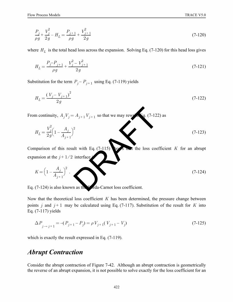
Flow Process Models TRACE V5.0
(7-120)
where is the total head loss across the expansion. Solving Eq. (7-120) for this head loss gives
(7-121)
Substitution for the term using Eq. (7-119) yields
(7-122)
From continuity, so that we may rewrite Eq. (7-122) as
(7-123)
Comparison of this result with Eq. (7-115) shows that the loss coefficient for an abrupt
expansion at the interface is
. (7-124)
Eq. (7-124) is also known as the Borda-Carnot loss coefficient.
Now that the theoretical loss coefficient has been determined, the pressure change betweenpoints and may be calculated using Eq. (7-117). Substitution of the result for intoEq. (7-117) yields
(7-125)
which is exactly the result expressed in Eq. (7-119).
Abrupt Contraction
Consider the abrupt contraction of Figure 7-42. Although an abrupt contraction is geometricallythe reverse of an abrupt expansion, it is not possible to solve exactly for the loss coefficient for an
Pjρg------
Vj2
2g------ HL–+
Pj 1+ρg
------------Vj 1+
2
2g-------------+=
HL
HLPj P– j 1+
ρg---------------------
Vj2 Vj 1+
2–2g
--------------------------+=
Pj Pj 1+–
HLVj Vj 1+–( )2
2g--------------------------------=
AjVj Aj 1+ Vj 1+=
HLVj
2
2g------ 1
AjAj 1+-------------–⎝ ⎠
⎛ ⎞ 2=
K
j 1 2⁄+
K 1Aj
Aj 1+-------------–⎝ ⎠
⎛ ⎞ 2=
Kj j 1+ K
∆Pj j 1+→
Pj 1+ Pj–( )–= ρVj 1+ Vj 1+ Vj–( )=
DRAFT
422
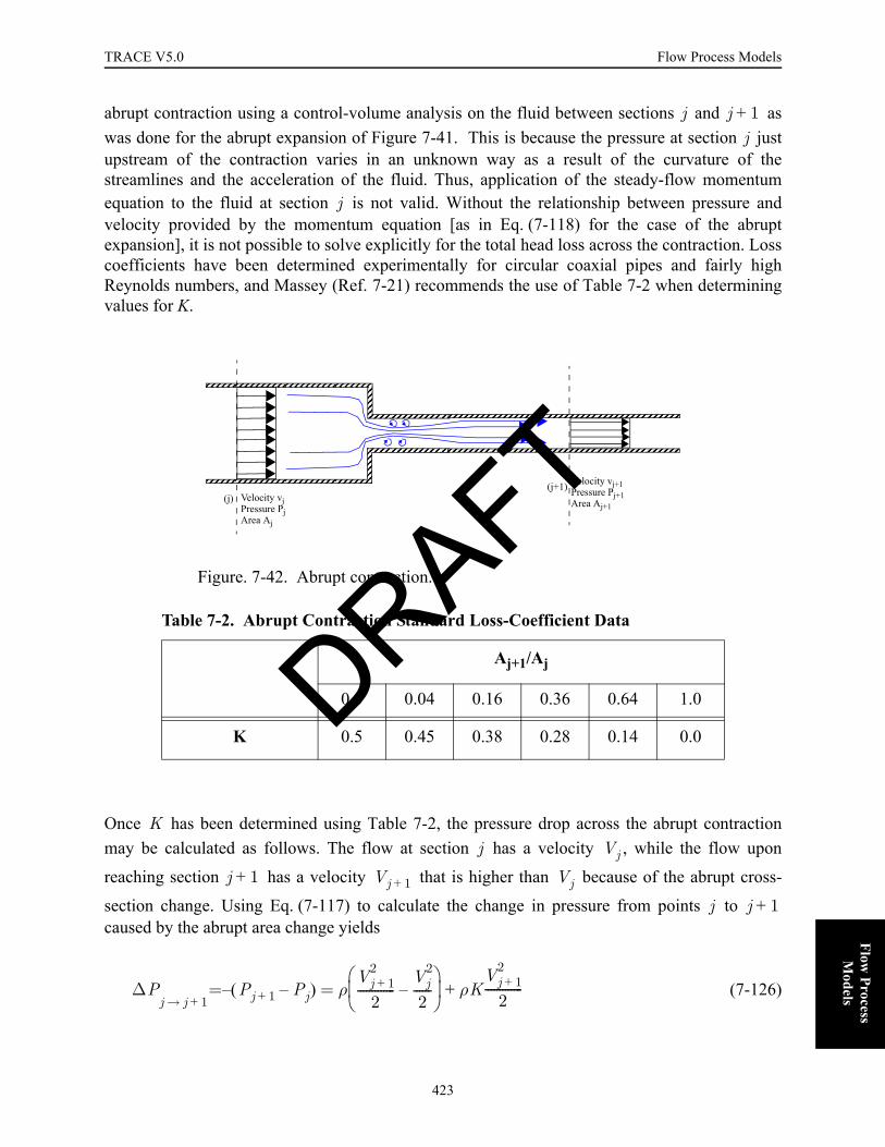
TRACE V5.0 Flow Process Models FOOBAR1234FOOBAR1234FOOBAR1234FOOBAR1234FOOBAR1234FOOBAR1234
Flow Process
Models
abrupt contraction using a control-volume analysis on the fluid between sections and aswas done for the abrupt expansion of Figure 7-41. This is because the pressure at section justupstream of the contraction varies in an unknown way as a result of the curvature of thestreamlines and the acceleration of the fluid. Thus, application of the steady-flow momentumequation to the fluid at section is not valid. Without the relationship between pressure andvelocity provided by the momentum equation [as in Eq. (7-118) for the case of the abruptexpansion], it is not possible to solve explicitly for the total head loss across the contraction. Losscoefficients have been determined experimentally for circular coaxial pipes and fairly highReynolds numbers, and Massey (Ref. 7-21) recommends the use of Table 7-2 when determiningvalues for K.
Once has been determined using Table 7-2, the pressure drop across the abrupt contractionmay be calculated as follows. The flow at section has a velocity , while the flow upon
reaching section has a velocity that is higher than because of the abrupt cross-
section change. Using Eq. (7-117) to calculate the change in pressure from points to caused by the abrupt area change yields
(7-126)
Figure. 7-42. Abrupt contraction.
Table 7-2. Abrupt Contraction Standard Loss-Coefficient Data
Aj+1/Aj
0.0 0.04 0.16 0.36 0.64 1.0
K 0.5 0.45 0.38 0.28 0.14 0.0
j j 1+j
j
(j) Velocity vjPressure PjArea Aj
(j+1) Velocity vj+1Pressure Pj+1Area Aj+1
Kj Vj
j 1+ Vj 1+ Vj
j j 1+
∆Pj j 1+→
Pj 1+ Pj–( )–= ρVj 1+
2
2-------------
Vj2
2------–
⎝ ⎠⎜ ⎟⎛ ⎞
ρKVj 1+
2
2-------------+=
DRAFT
423

Flow Process Models TRACE V5.0
where is taken from Table 7-2
Thin-Plate Orifice
As in the case of the abrupt contraction, it is not possible to determine theoretically the losscoefficient across a thin-plate orifice, so experimental data must be used. For a sharp-edged, thin-plate orifice in a straight conduit, as shown in Figure 7-43, Idel’Chik (Ref. 7-18) suggests that thefollowing expression be used for the loss coefficient in the presence of high Reynolds numberflow (≥ 105):
(7-127)
This curve fit also agrees well with the data plotted in White (Ref. 7-22) for the irrecoverable headloss across a thin-plate orifice.
Once the loss coefficient for a sharp-edged, thin-plate orifice has been determined usingEq. (7-127), the pressure drop across the orifice may be calculated as follows. The flow at section
has a velocity , while the flow upon reaching section has a velocity , which
Figure. 7-43. Sharp-edged, thin-plate orifice.
K
K
Vj Vj+1/2 Vj+1
(j) (j+1/2) (j+1)
Pressure pj Pressure pj+1/2 Pressure pj+1Area Aj Area Aj+1/2 Area Aj+1
K 1 0.707 1A
j 1 2⁄+
Aj------------------–
Aj 1 2⁄+
Aj------------------–+
⎝ ⎠⎜ ⎟⎛ ⎞
2
=
K
j Vj j 1 2⁄+ Vj 1 2⁄+
DRAFT
424
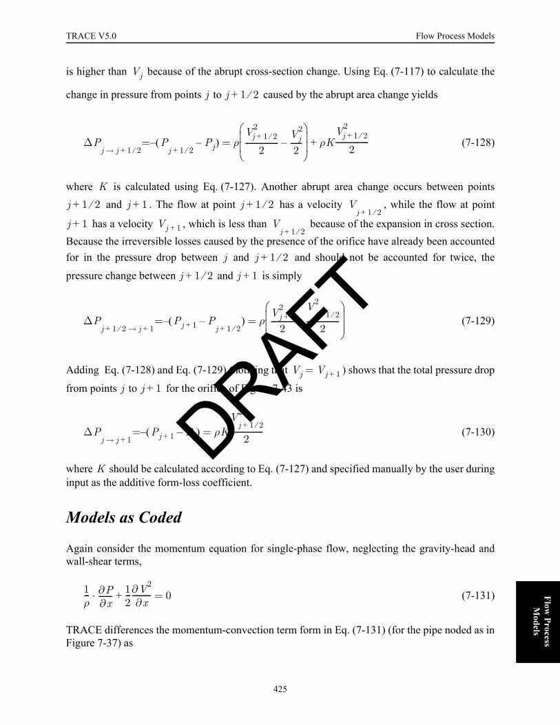
TRACE V5.0 Flow Process Models FOOBAR1234FOOBAR1234FOOBAR1234FOOBAR1234FOOBAR1234FOOBAR1234
Flow Process
Models
is higher than because of the abrupt cross-section change. Using Eq. (7-117) to calculate the
change in pressure from points to caused by the abrupt area change yields
(7-128)
where is calculated using Eq. (7-127). Another abrupt area change occurs between points and . The flow at point has a velocity , while the flow at point
has a velocity , which is less than because of the expansion in cross section.Because the irreversible losses caused by the presence of the orifice have already been accountedfor in the pressure drop between and and should not be accounted for twice, the
pressure change between and is simply
(7-129)
Adding Eq. (7-128) and Eq. (7-129) (noticing that ) shows that the total pressure drop
from points to for the orifice of Figure 7-43 is
(7-130)
where should be calculated according to Eq. (7-127) and specified manually by the user duringinput as the additive form-loss coefficient.
Models as Coded
Again consider the momentum equation for single-phase flow, neglecting the gravity-head andwall-shear terms,
(7-131)
TRACE differences the momentum-convection term form in Eq. (7-131) (for the pipe noded as inFigure 7-37) as
Vj
j j 1 2⁄+
∆Pj j 1 2⁄+→
Pj 1 2⁄+
Pj–( )–= ρVj 1 2⁄+
2
2------------------
Vj2
2------–
⎝ ⎠⎜ ⎟⎜ ⎟⎛ ⎞
ρKVj 1 2⁄+
2
2------------------+=
K
j 1 2⁄+ j 1+ j 1 2⁄+ Vj 1 2⁄+
j 1+ Vj 1+ Vj 1 2⁄+
j j 1 2⁄+
j 1 2⁄+ j 1+
∆Pj 1 2⁄+ j 1+→
Pj 1+ Pj 1 2⁄+
–( )–= ρVj 1+
2
2-------------
Vj 1 2⁄+2
2------------------–
⎝ ⎠⎜ ⎟⎜ ⎟⎛ ⎞
=
Vj Vj 1+=
j j 1+
∆Pj j 1+→
Pj 1+ Pj–( )–= ρKV
j 1 2⁄+2
2------------------=
K
1ρ--- ∂P
∂x------- 1
2---∂V2
∂x----------+ 0=·
DRAFT
425

Flow Process Models TRACE V5.0
(7-132)
Written in terms of a pressure drop between points j and j + 1,
. (7-133)
This finite-difference result is identical to the integral result of Eq. (7-113).
As before, if no area change occurs between points and , the velocity of the flow does notchange, and Eq. (7-133) predicts
(7-134)
as expected. If an abrupt area change between sections and does occur, however, then aform-loss factor is again added to the pressure-drop equation to account for irreversible losses.This yields the general equation for a pressure drop between point and when an abruptarea change is present, such that,
(7-135)
where is the cell-edge velocity at the location of the area change.
In TRACE, pressures are cell-centered quantities whereas velocities are cell-edge quantities.Therefore, approximating the cell-centered velocities in Eq. (7-135) by donoring the interfacevelocities and assuming continuity of volumetric flow gives for a positive-direction flow velocity,
(7-136)
Because the pressure-drop equation in TRACE is identical in form to Eq. (7-117), the losscoefficient calculated by TRACE is exactly that developed in the previous pages for thecases of abrupt expansion and contraction. Namely, for an abrupt expansion noded as in Figure7-39, TRACE calculates the loss coefficient as
(7-137)
1ρ--- pj 1+ pj–( ) 0.5 Vj 1+
2 Vj2–( )+ 0=
pj j 1+( )→
∆ pj 1+ pj–( )– 0.5ρ Vj 1+2 Vj
2–( )= =
j j 1+
pj j 1+→
∆ 0=
j j 1+
j j 1+
pj j 1+→
∆ pj 1+ pj–( )– 0.5ρ Vj 1+2 Vj
2–( ) 0.5KTRACEρVs2+= =
Vs
pj 1+∆ pj 1+ pj–( )– 0.5ρA
j 12---+
Aj 1+-------------
Aj 1
2---+
Aj-------------+ V
j 12---+
Aj 1
2---+
Aj 1+-------------V
j 12---+
Aj 1
2---–
Aj-------------V
j 12---–
–= =
KTRACE
KTRACE 1Aj
Aj 1+-------------–⎝ ⎠
⎛ ⎞ 2 Aj 1 2⁄+
Aj------------------
⎝ ⎠⎜ ⎟⎛ ⎞
2
=
DRAFT
426

TRACE V5.0 Flow Process Models FOOBAR1234FOOBAR1234FOOBAR1234FOOBAR1234FOOBAR1234FOOBAR1234
Flow Process
Models
The factor (1−Aj/Aj+1)2 is the K-factor to be applied to the minimum flow-area-velocity squared,
, as presented in Eq. (7-124). The other factor (Aj+1/2/Aj)2 converts that K-factor to ,
which is applied to the mesh-cell interface-velocity squared, . This conversion is based on
assuming continuity of volumetric flow; i.e., AjVj = Aj+1⁄2 Vj+1⁄2. Similarly, the loss coefficient foran abrupt contraction noded as in Figure 7-38 is calculated by TRACE as a curve fit to the data ofTable 7-2, such that
(7-138)
The bracketed factor is the -factor to be applied to the minimum flow-area-velocity
Multiplying by the following factor (Aj+1/2/Aj+1)2 defines to be applied to the mesh-cell
interface-velocity squared, .
TRACE is programmed also to add abrupt flow-area change losses to the 3D VESSELcomponent. Because NFF is not a VESSEL-component input parameter, the negative values forthe liquid additive friction-loss coefficients CFZL-T, CFZL-Z, and CFZL-R are used as a user-defined input flag that turns on the 3D abrupt area change model. TRACE evaluates the sameabrupt flow-area change loss and adds it to the absolute value of the input-specified additivefriction-loss coefficient. This is done for both liquid and vapor and forward and reverse flow. Thevolume-averaged flow area in the radial direction for cylindrical geometry is divided by
[that is, ] to remove the smooth flow-
area change effect from cylindrical geometry.
References7-1 M. S. Sahota and J. F. Lime, "TRAC-PF1 Choked Flow Model", Los Alamos National
Laboratory Report LA-UR-82-1666, also CONF-830103-8, Submitted to SecondInternational Topical Meeting on Nuclear Reactor Thermal-Hydraulics, (Santa Barbara,California, January 1983).
7-2 J. W. Burnell, “Flow of Boiling Water through Nozzles, Orifices, and Pipes,” Engineering,pp. 572-576, (1947).
7-3 “RELAP5/MOD1 Code Manual, Volume 1: System Models and Numerical Methods,”Idaho National Engineering Laboratory report EGG-2070 Draft, Rev. 1, also NUREG/CR-1826 (March 1981).
Vj2 KTRACE
Vj 1 2⁄+2
KTRACE 0.5 0.7Aj 1+Aj
-------------⎝ ⎠⎛ ⎞– 0.2
Aj 1+Aj
-------------⎝ ⎠⎛ ⎞
2+
⎩ ⎭⎨ ⎬⎧ ⎫
Aj 1 2⁄+
Aj 1+------------------
⎝ ⎠⎜ ⎟⎛ ⎞
2
=
K Vj 1+2
KTRACE
Vj 1 2⁄+2
RmeanjRinj Routj+
2-----------------------------= ∆θj R· meani ∆ri ∆zk· · volijk=DRAFT
427

Flow Process Models TRACE V5.0
7-4 M. D. Alamgir and J. H. Lienhard, “Correlation of Pressure Undershoot During Hot WaterDepressurization,” Transactions of ASME, Journal of Heat Transfer, 103, pp. 52-73,(1981).
7-5 O. C. Jones, Jr., “Flashing Inception in Flowing Liquids,” Brookhaven NationalLaboratory report BNL-NUREG-51221, also NUREG/CR-1515, (1980).
7-6 N. Abuaf, O. C. Jones, Jr., and B. J. C. Wu, "Critical Flashing Flow in Nozzles withSubcooled Inlet Conditions", BNL-NUREG-27512, Brookhaven National Laboratory,1980.
7-7 V. H. Ransom and J. A. Trapp, “The RELAP5 Choked Flow Model and Application to aLarge Scale Flow Test,” in ANS/ASME/NRC International Topical Meeting on NuclearReactor Thermal-Hydraulics (Saratoga Springs, New York, 1980), pp. 799–819.
7-8 F. M. White, Fluid Mechanics (McGraw-Hill, Inc., New York, 1979), p 515.
7-9 G. B. Wallis, One Dimensional Two Phase Flow (McGraw-Hill Book Company,New York, 1969).
7-10 S. S. Kutateladze, Izv. Akad. Nauk SSSR, Otd. Tekhn. Nauk, Vol. 8, p. 529 (1951).
7-11 S. G. Bankoff, R. S. Tankin, M. C. Yuen, and C. L. Hsieh, “Countercurrent Flow of Air/Water and Steam/Water through a Horizontal Perforated Plate,” International Journal ofHeat and Mass Transfer, 24:8, pp. 1381–1395 (1981).
7-12 L. A. Crotzer, “TRAC-PF1/MOD2 TEE Component Offtake Model: A CompletionReport,” Los Alamos National Laboratory report LA-UR-91-4052 (November 1991).
7-13 K. H. Ardron and W. M. Bryce, “Assessment of Horizontal Stratification EntrainmentModel in RELAP5/MOD2,” United Kingdom Atomic Energy Authority, AEE Winfrithdraft report AEEW-R 2345 (April 1988).
7-14 C. Smoglie, “Two Phase Flow Through Small Break Branches in a Horizontal Pipe withStratified Flow,” Kernforschungszentrum Karlsruhe report KfK 3861 (December 1984).
7-15 V. E. Schrock, S. T. Revankar, R. Mannheimer, and C. H. Wang, “Small Break CriticalDischarge—The Roles of Vapor and Liquid Entrainment in a Stratified Two-Phase RegionUpstream of the Break,” Lawrence Berkeley Laboratory report LBL-22024 (NUREG/CR-4761) (December 1986).
7-16 T. Maciaszek and A. Menponteil, “Experimental Study on Phase Separation in a TeeJunction for Steam-Water Stratified Inlet Flow,” European Two-Phase Flow GroupMeeting, Munich, Germany, June 10-13, 1986.
DRAFT
428

TRACE V5.0 Flow Process Models FOOBAR1234FOOBAR1234FOOBAR1234FOOBAR1234FOOBAR1234FOOBAR1234
Flow Process
Models
7-17 J. L. Anderson and R. L. Benedetti, “Critical Flow Through Small Pipe Breaks,” ElectricPower Research Institute report EPRI NP-4532 (May 1986).
7-18 I. E. Idel’Chik, Handbook of Hydraulic Resistance, Coefficients of Local Resistance andof Friction, National Technical Information Service Report NTIS AEC-TR-6630, p. 139,(1960).
7-19 “Flow of Fluids through Valves, Fittings, and Pipes,” Metric Edition-SI Units of the CraneManual, Technical Paper No. 410M, Crane Co., New York (1977).
7-20 R. C. Blevins, Applied Fluid Dynamics Handbook (Krieger Publishing Co., Malabar,Florida, 1992).
7-21 B. S. Massey, Mechanics of Fluids (D. Van Nostrand Co., New York, 1968), pp. 217-219.
7-22 F. M. White, Fluid Mechanics (McGraw-Hill Book Co., New York, 1979), p. 384.
7-23 Ransom, V., “Numerical Benchmark Test No. 2.2: Oscillating Manometer,” MultiphaseScience and Technology, 6, Hemisphere Publishing, New York (1992), 591-609.
7-24 B. Aktas, "Level Tracking in Thermal-Hydraulic Simulations of Nuclear Reactors", Ph.D.Thesis, The Pennsylvania State University, State College, PA (2003)
DRAFT
429

Flow Process Models TRACE V5.0
DRAFT
430

Fuel Rod
Models
8Fuel Rod ModelsFOOBAR1234
TRACE includes an extensive library of temperature dependent material properties that enables itto model a wide variety of structural materials commonly used in reactor systems and testfacilities. Of particular interest in reactor safety however, are the material properties andadditional models that are specific to nuclear fuel rods. This section describes the properties andmodels used by TRACE to represent nuclear fuel and cladding materials. Included are sections todescribe models and correlations for UO2 and mixed oxide fuel thermal expansion, thermalconductivity, specific heat, density, and spectral emissivity for use in the heat-transfercalculations.
Correlations for Zircaloy cladding, Zircaloy dioxide, and fuel-cladding gap gases are alsodescribed. Because at high temperatures Zircaloy-based cladding can undergo an exothermicchemical reaction with steam, models for cladding oxidation and metal-water reaction arediscussed in this section as well.
The TRACE materials library uses numerical indexes for each specific material. The materialindexes in the TRACE library that apply to fuel and cladding are:
1 – mixed-oxide fuel; 2 – Zircaloy; 3 – fuel-clad gap gases; and11 – Zircaloy dioxide.
Since there is no appreciable difference in material properties between conventional Zircaloycladding and newer materials such as Zirlo and M5, TRACE uses the same material properties forall cladding types. While all properties include an emissivity for doing a radiative-heat-transfercalculation, the calculation is only done in connection with the gap-conductivity calculation. Thefilm-boiling heat-transfer model also includes a radiative-heat-transfer calculation, but theemissivity is specified in connection with that model.
NomenclatureThe following nomenclature is used in this section:
DRAFT
431

Fuel Rod Models TRACE V5.0
= specific heat capacity at constant pressure (J/kg-K)
= total gas gap heat transfer coefficient
= gap-gas conductance
= fuel-cladding interfacial contact resistance
= fuel-to-cladding thermal radiation heat transfer coefficient
= Boltzmann’s constant (J/K) or thermal conductivity (W/m-K)
= gap-mixture thermal conductivity
= linear strain caused by thermal expansion
= molecular weight
= pressure (Pa)
= gap-gas pressure
= temperature (K)
= temperature (°C)
= temperature (°F)
= reference temperature (K) for gas gap calculation
= fuel centerline temperature
= fuel surface temperature
= fuel temperature
= cladding temperature
= cladding outside temperature
= cladding inside temperature
= average gap gas temperature
= mole fraction
= fraction of theoretical fuel density
= weight fraction of PuO2 in the fuel
= weight fraction of UO2 in the fuel
= reacting surface radius (m)
cp
hgap
hgas
hcontact
hradiation
k
kgap
L∆ L0⁄
M
p
pgap
T
TC
TF
TREF
Tcl
Tsurf
Tf
Tc
Tco
Tcl
Tgap
x
fTD
fPuO2
fUO2
r
DRAFT
432

TRACE V5.0 Fuel Rod Models
Fuel Rod
Models
= mass per unit length of zirconium consumed in metal-water reaction
= heat source added to conduction equation from metal-water reaction
= fuel-cladding radial gas gap distance
= cladding outer surface radius (m)
, = radius of the outer fuel surface
, = radius to the inner cladding surface
= radial displacement of a fuel region
Greek = linear thermal-expansion coefficient
= characteristic dimension for a closed gap
= initial, undeformed radial thickness of cracked fuel
= cracked fuel deformed thickness
= radial gap width after thermal expansion of fuel and cladding
= thickness of zirconium oxide layer
= emissivity
= fuel emissivity
= cladding surface emissivity
, , = parameters in metal-water reaction model
= characteristic fuel RMS roughness
= Poisson’s ration
= density (kg/m3)
= density of zirconium oxide (kg/m3)
= Stefan-Boltzmann constant (W/m2/K4)
= kinetic parameter representing total oxygen consumed (kg/m2)
Subscripts = cladding
= centerline
= fuel
m'Zr
q'''mw
rgap∆
Ro
Rf Rf∗
Rc RI
u r( )
α
δr
δo
δcf
δgap
δZrO2
ε
εf
εw
η1 η2 η3
λ
ν
ρ
ρZrO2
σSB
τ
c
cl
f
DRAFT
433
Fuel Rod Models TRACE V5.0
=cracked fuel
= gas gap
= i-th constituent gas
= j-th constituent gas
= value after thermal expansion
= radial direction
= steam
= surface
= axial direction
Superscripts = time step
= time-step increment
Nuclear Fuel Mixed-Oxide Properties TRACE calculates the properties for mixed-oxide (UO2 and PuO2) nuclear fuels. Thevalues determined by TRACE are dependent on three input variables: the fraction oftheoretical density, the fraction of plutonium dioxide in the fuel, and the fuel burnup.Property changes upon melting are not included in this code version.
Fuel Density
The model for fuel density in TRACE accounts for dimensional changes in the fuel pellets due totemperature. Dimensional changes affect the pellet to cladding gap size, which in turn affects thegap heat transfer and stored energy of the fuel in a safety analysis. The model is valid for UO2,PuO2, and their mixed oxides. Fuel density is calculated with a correction factor to account forthermal expansion, which is assumed to be axisymmetric, as
(8-1)
where
= density (kg/m3)
cf
gap
i
j
new
r
steam
surf
z
n
n 1+
ρfTD 1 fPuO2
–( )ρUO2fPuO2
ρPuO2+[ ]
1 3 L∆L0-------+⎝ ⎠
⎛ ⎞----------------------------------------------------------------------------------------=
ρ
DRAFT
434
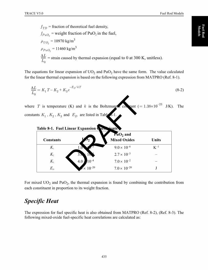
TRACE V5.0 Fuel Rod Models
Fuel Rod
Models
= fraction of theoretical fuel density,
= weight fraction of PuO2 in the fuel,
= 10970 kg/m3
= 11460 kg/m3
= strain caused by thermal expansion (equal to 0 at 300 K, unitless).
The equations for linear expansion of UO2 and PuO2 have the same form. The value calculatedfor the linear thermal expansion is based on the following expression from MATPRO (Ref. 8-1).
(8-2)
where is temperature (K) and is the Boltzmann's constant ( J/K). The
constants and are listed in Table 8-1.
For mixed UO2 and PuO2, the thermal expansion is found by combining the contribution fromeach constituent in proportion to its weight fraction.
Specific Heat
The expression for fuel specific heat is also obtained from MATPRO (Ref. 8-2), (Ref. 8-3). Thefollowing mixed-oxide fuel-specific heat correlations are calculated as:
Table 8-1. Fuel Linear Expansion Coefficients
Constants UO2
PuO2 andMixed Oxides Units
K1 1.0 × 10⁻⁵ 9.0 × 10⁻⁶ K–1
K2 3.0 × 10⁻³ 2.7 × 10⁻³ –
K3 4.0 × 10⁻⁴ 7.0 × 10⁻² –
ED 6.9 × 10⁻²⁰ 7.0 × 10⁻²⁰ J
fTD
fPuO2
ρUO2
ρPuO2
L∆L0-------
L∆L0------- K1T K2– K3e
ED kT⁄–+=
T k 1.38 23–×10=
K1 K2 K3, , ED
DRAFT
435

Fuel Rod Models TRACE V5.0
(8-3)
where = specific heat capacity (J/kg-K). The constants through , are listed in Table8-2.
Fuel Thermal Conductivity
The thermal conductivity of UO2 and mixed oxides is a fit to data. The fuel thermal conductivitycorrelations are taken from the MATPRO (Ref. 8-2). Separate correlations are employed for
temperatures deg C, and deg C. The break between the low andhigh temperature regions depends on the oxide. Both expressions include correction factors toaccount for porosity and density.
For
(8-4)
and for ,
(8-5)
where, is in degrees Celsius and is the porosity correction factor.
Table 8-2. Fuel Specific Heat CoefficientsConstants Uranium Dioxide Mixed Oxides
b1 19.145 19.53b2 7.8473 × 10⁻⁴ 9.25 × 10⁻⁴
b3 5.6437 × 10⁶ 6.02 × 10⁶
b4 535.285 539.0b5 37694.6 40100.0b6 1.987 1.987
cP 15.496b1b4
2 b4 T⁄( )exp
T2 b4 T⁄( )exp 1–[ ]2
---------------------------------------------------- 2b2Tb3b5
b6T2------------ b5 b6T⁄–( )exp+ +
⎩ ⎭⎪ ⎪⎨ ⎬⎪ ⎪⎧ ⎫
=
cP b1 b6
0 TC TL≤< TL TC 2840< <
TC TL<
k cc1
c2 TC+------------------- c3 c4TC( )exp+=
TC TL>
k c c5 c3 c4TC( )exp+[ ]=
TC c
DRAFT
436

TRACE V5.0 Fuel Rod Models
Fuel Rod
Models
For PuO2 and mixed oxides the correction factor for porosity is given by:
(8-6)
and for UO2 it is given by:
(8-7)
In these expressions, is the fraction of theoretical fuel density and
(8-8)
The constants through , and the transition temperature are listed in Table 8-3.
Fuel Spectral Emissivity
The spectral emissivity of the fuel is used in calculation of the fuel to cladding heat conductance,which is described in a later section. Above approximately 1000 K the emissivity of reactor fueldecreases with temperature, and then becomes constant above about 2050 K. The correlationsused in TRACE were obtained from MATPRO (Ref. 8-2). In these correlations, the spectralemissivity of both uranium dioxide and mixed oxide fuel is modeled as a linear function oftemperature between 1000 and 2050 K. Outside this range, the emissivity is assumed to beindependent of temperature. Eq. (8-9) lists the temperature range and spectral emissivity andFigure 8-1 compares the calculated emissivity with data by Claudson (Ref. 8-8) and Ehlert andMargrave (Ref. 8-9)..
Table 8-3. Fuel Thermal Conductivity Equation CoefficientsConstants Uranium Dioxide Mixed Oxides
c1 40.4 33.0c2 464.0 375.0c3 1.216 × 10⁻⁴ 1.54 × 10⁻⁴
c4 1.867 × 10⁻³ 1.71 × 10⁻³
c5 0.0191 0.0171c6 2.58 1.43c7 –5.8 × 10⁻⁴ 0.0
TL (°C) 1650.0 1550.0
c 100.0fTD
1 β 1 fTD–( )–----------------------------------- 1 0.04β+
0.96-----------------------⎝ ⎠
⎛ ⎞=
c 100.01 β 1 fTD–( )–
1 0.05β–-----------------------------------=
fTD
β c6 c7TC+=
c1 c7 TL
DRAFT
437
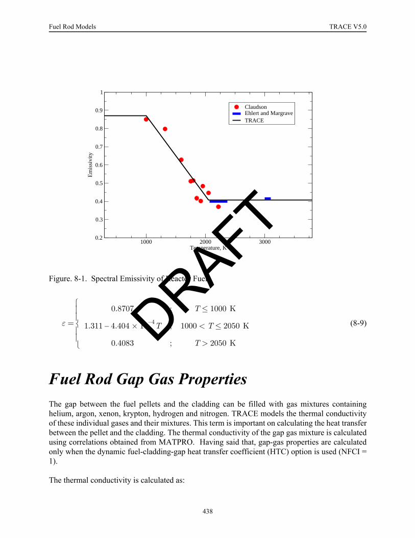
Fuel Rod Models TRACE V5.0
(8-9)
Fuel Rod Gap Gas PropertiesThe gap between the fuel pellets and the cladding can be filled with gas mixtures containinghelium, argon, xenon, krypton, hydrogen and nitrogen. TRACE models the thermal conductivityof these individual gases and their mixtures. This term is important on calculating the heat transferbetween the pellet and the cladding. The thermal conductivity of the gap gas mixture is calculatedusing correlations obtained from MATPRO. Having said that, gap-gas properties are calculatedonly when the dynamic fuel-cladding-gap heat transfer coefficient (HTC) option is used (NFCI =1).
The thermal conductivity is calculated as:
Figure. 8-1. Spectral Emissivity of Reactor Fuel
1000 2000 3000Temperature, K
0.2
0.3
0.4
0.5
0.6
0.7
0.8
0.9
1E
mis
sivi
ty
ClaudsonEhlert and MargraveTRACE
ε
0.8707 ; T 1000 K≤
1.311 4.404 10 4–× T– ; 1000 T 2050 K≤<
0.4083 ; T 2050 K>⎩⎪⎪⎨⎪⎪⎧
= DRAFT
438
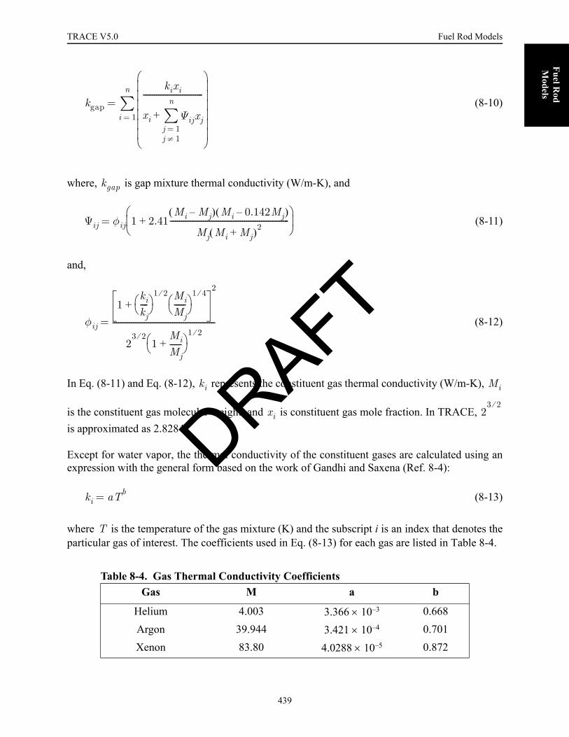
TRACE V5.0 Fuel Rod Models
Fuel Rod
Models
(8-10)
where, is gap mixture thermal conductivity (W/m-K), and
(8-11)
and,
(8-12)
In Eq. (8-11) and Eq. (8-12), represents the constituent gas thermal conductivity (W/m-K),
is the constituent gas molecular weight, and is constituent gas mole fraction. In TRACE, is approximated as 2.8284.
Except for water vapor, the thermal conductivity of the constituent gases are calculated using anexpression with the general form based on the work of Gandhi and Saxena (Ref. 8-4):
(8-13)
where is the temperature of the gas mixture (K) and the subscript i is an index that denotes theparticular gas of interest. The coefficients used in Eq. (8-13) for each gas are listed in Table 8-4.
Table 8-4. Gas Thermal Conductivity CoefficientsGas M a b
Helium 4.003 3.366 × 10⁻³ 0.668Argon 39.944 3.421 × 10⁻⁴ 0.701Xenon 83.80 4.0288 × 10⁻⁵ 0.872
kgap
kixi
xi Ψijxjj 1=j 1≠
n
∑+
--------------------------------
⎝ ⎠⎜ ⎟⎜ ⎟⎜ ⎟⎜ ⎟⎜ ⎟⎜ ⎟⎛ ⎞
i 1=
n
∑=
kgap
Ψij φij 1 2.41Mi Mj–( ) Mi 0.142Mj–( )
Mj Mi Mj+( )2----------------------------------------------------------------+
⎝ ⎠⎜ ⎟⎛ ⎞
=
φij
1kikj----⎝ ⎠
⎛ ⎞1 2⁄ Mi
Mj------⎝ ⎠
⎛ ⎞1 4⁄
+2
23 2⁄
1MiMj------+⎝ ⎠
⎛ ⎞1 2⁄
-------------------------------------------------------=
ki Mi
xi 23 2⁄
ki aTb=
T
DRAFT
439
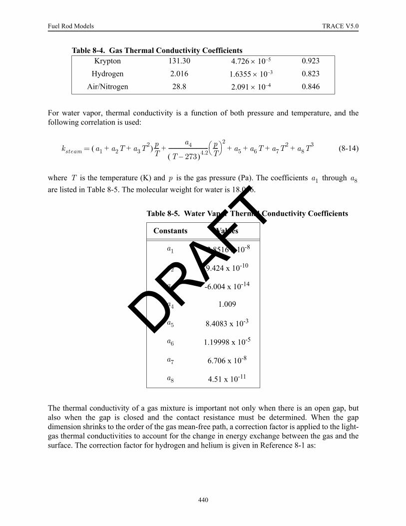
Fuel Rod Models TRACE V5.0
For water vapor, thermal conductivity is a function of both pressure and temperature, and thefollowing correlation is used:
(8-14)
where is the temperature (K) and is the gas pressure (Pa). The coefficients through are listed in Table 8-5. The molecular weight for water is 18.016.
The thermal conductivity of a gas mixture is important not only when there is an open gap, butalso when the gap is closed and the contact resistance must be determined. When the gapdimension shrinks to the order of the gas mean-free path, a correction factor is applied to the light-gas thermal conductivities to account for the change in energy exchange between the gas and thesurface. The correction factor for hydrogen and helium is given in Reference 8-1 as:
Krypton 131.30 4.726 × 10⁻⁵ 0.923Hydrogen 2.016 1.6355 × 10⁻³ 0.823
Air/Nitrogen 28.8 2.091 × 10⁻⁴ 0.846
Table 8-5. Water Vapor Thermal Conductivity Coefficients
Constants Values
-2.8516 x 10⁻⁸
9.424 x 10⁻¹⁰
-6.004 x 10⁻¹⁴
1.009
8.4083 x 10⁻³
1.19998 x 10⁻⁵
6.706 x 10⁻⁸
4.51 x 10⁻¹¹
Table 8-4. Gas Thermal Conductivity Coefficients
ksteam a1 a2T a3T2+ +( ) p
T----
a4
T 273–( )4.2------------------------------ p
T----⎝ ⎠
⎛ ⎞ 2a5 a6T a7T
2 a8T3+ + + + +=
T p a1 a8
a1
a2
a3
a4
a5
a6
a7
a8
DRAFT
440

TRACE V5.0 Fuel Rod Models
Fuel Rod
Models
(8-15)
where,
. (8-16)
In Eq. (8-16), is the average gap gas temperature (K), is the gap-gas pressure, and isthe characteristic fuel RMS roughness. Consistent with MATPRO, in TRACE the roughness is
assumed equal to m for commercial nuclear fuel. This correction is only made forhydrogen and helium. No correction is applied to the other component gases.
Zircaloy Cladding PropertiesTRACE calculates the properties for Zircaloy and oxidized Zircaloy cladding. TRACE assumesthe properties for all common Zircaloy based alloys; Zircaloy-2, Zircaloy-4, Zirlo, M5, E110, etc.to be identical. The only difference in properties between Zircaloy and oxidized Zircaloy is in thethermal conductivity. The equations used are based on the correlations in MATPRO (Ref. 8-1)and/or FRAPTRAN (Ref. 8-11).
Cladding Density
Zircaloy cladding exhibits an asymmetric thermal-expansion behavior. Thermal expansion iscalculated in the radial and axial directions, and these effects are included in the densitycalculation as follows:
(8-17)
where, for K
(8-18)
and,
kki
1 f ki+----------------=
f0.2103 Tgap
pgapλ--------------------------------=
Tgap pgap λ
4.389 6–×10
ρ 6551.4
1 2 L∆L
-------⎝ ⎠⎛ ⎞
r
L∆L
-------⎝ ⎠⎛ ⎞
z++
-------------------------------------------------------=
T 1073.15≤
L∆L
-------⎝ ⎠⎛ ⎞
r2.373 4–×10– 6.721 6–×10 TC+=
DRAFT
441

Fuel Rod Models TRACE V5.0
(8-19)
For ,
(8-20)
and,
(8-21)
and, for K:
(8-22)
and
(8-23)
In Equations (8-18) through (8-23), = temperature (K) and = temperature (oC).
Cladding Specific Heat
The specific heat for all Zircaloy based alloys is obtained by linear interpolation of values listed inTable 8-6. This is the same table of values used by FRAPTRAN (Ref. 8-11), and represents a fitto several sets of experimental data. Below 1090 K the table values are based on data obtained byBrooks and Stansbury (Ref. 8-12). The standard error for data in this low temperature range is
reported to be 1.1 J/kg-K for K and 2.8 J/kg-K for temperatures between
and K. Because Zircaloy undergoes a phase change (alpha to beta) from 1090 to 1248 K,there is a resultant sharp spike in the specific-heat values during the transition, as shown in Figure8-2. The specific heat values in this transition region are based on data by Deem and Eldridge
L∆L
-------⎝ ⎠⎛ ⎞
z2.506 6–×10– 4.441 6–×10 TC+=
1073.15 T< 1273.15≤
L∆L
-------⎝ ⎠⎛ ⎞
r5.1395 3–×10 1.12 5–×10 T 1073.15–( )–=
L∆L
-------⎝ ⎠⎛ ⎞
z3.5277 3–×10 1.06385 5–×10– 4.441 6–×10( )TC=
T 1273.15>
L∆L
-------⎝ ⎠⎛ ⎞
r6.8 3–×10– 9.7 6–×10 TC+=
L∆L
-------⎝ ⎠⎛ ⎞
z8.3 3–×10– 9.7 6–×10 TC+=
T TC
300 T 800< < 800
1090
DRAFT
442

TRACE V5.0 Fuel Rod Models
Fuel Rod
Models
(Ref. 8-13), with a standard error of 10.7 J/kg-K. For temperatures greater than 1248 K, a constantvalue of = 356 J/kg-K is assigned.
Cladding Thermal Conductivity
The thermal conductivity of Zircaloy is based on a fit to experimental data that included both Zr-2 and Zr-4. It is assumed that this conductivity is applicable to all Zircaloy based cladding. Thecorrelation for Zircaloy thermal conductivity and its database is discussed in Reference (Ref. 8-11). For Zircaloy, the thermal conductivity is given by:
(8-24)
The standard deviation of this correlation is reported to be W/m-K. This correlation shouldbe used for temperatures below K.
For zirconium dioxide, the following expression is used for thermal conductivity:
Table 8-6. Zircaloy Specific Heat vs. Temperature for the α Phase and the Transition to the β Phase
T (K) cp (J/kg-K)
300 281
400 302
640 381
1090 375
1093 502
1113 590
1133 615
1153 719
1173 816
1193 770
1213 619
1233 469
1248 356
cp
kZr 7.51 2.09 2–×10( )T 1.45 5–×10( )T 2 7.67 9–×10( )T 3+–+=
1.011800
DRAFT
443

Fuel Rod Models TRACE V5.0
(8-25)
The temperature in both Equations (8-24) and (8-25) is in degrees Kelvin.
Cladding Spectral Emissivity
The emissivity of Zircaloy cladding depends on both temperature and thickness of the oxide layer
on the surface of the cladding. For oxide layers less than m, the emissivity can beestimated by (Ref. 8-11),
(8-26)
where is the thickness of the zirconium oxide layer in meters.
For fresh fuel with low burnup, the oxide thickness is small and the emissivity is nominally 0.4.
However, the emissivity increases with oxide thickness so that for layers exceeding m
Figure. 8-2. Specific Heat for Zircaloy Based Cladding Materials.
200 400 600 800 1000 1200 1400 1600 1800 2000Temperature, K
200
300
400
500
600
700
800
900Sp
ecif
ic H
eat,
J/kg
-K
kZrO21.96 2.41 4–×10( )– T 6.43 7–×10( )T2 1.95 10–×10( )– T3+=
3.88 6–×10
ε 0.325 0.1246 6×10( )δZrO2+=
δZrO2
3.88 6–×10
DRAFT
444

TRACE V5.0 Fuel Rod Models
Fuel Rod
Models
in thickness the emissivity exceeds 0.8. TRACE does not model the variation of emissivity with
oxide thickness, but simply assigns a constant value of . Figure 8-3 shows several setsof experimental data for zirconium oxide and the value used by TRACE.
Fuel-Cladding Gap Conductance The fuel-cladding gap conductance is a function of three components: the gap-gas conductance,fuel-cladding interfacial contact resistance, and fuel to cladding thermal radiation. In TRACE, atotal gap heat transfer coefficient is defined as the sum of the heat transfer coefficients foreach of these three components:
(8-27)
where,
Figure. 8-3. Emissivity of zirconium oxide.
ε 0.75=
400 600 800 1000 1200 1400Temperature, K
0.5
0.6
0.7
0.8
0.9
1
Em
issi
vity
Uniform Oxide; 10e-6 mUniform Oxide; 28e-6 mNodular Oxide; 130e-6 mCrud; 35e-6 mTRACE
hgap
hgap hgas hcontact hradiation+ +=
DRAFT
445

Fuel Rod Models TRACE V5.0
(8-28)
(8-29)
The view factor between the fuel and cladding assumes thermal radiation between two gray,diffuse, infinitely long concentric cylinders, and:
(8-30)
In Equations (8-28) through (8-30), is the gap-gas thermal conductivity, and and are the temperatures at the fuel outer surface and cladding inner surface at radii and, respectively. The fuel and cladding surface emissivities are and , respectively,
and is the Stefan-Boltzmann constant (= W/m2/K4). The characteristic
dimension for a closed gap is m, which accounts for the mean surfaceroughness of the fuel and the cladding plus the temperature jump distances. The contactconductance, is assumed to be zero.
Fuel - Cladding Gap Dimension
The fuel-cladding radial gas gap, , is found by using the uncoupled, quasi-staticapproximation (Ref. 8-7). In this approximation, the mechanical coupling term in the energyequation and the inertial term in the mechanical force balance are omitted. By neglecting theseterms, we assume that the fuel-cladding strains minimally affect the temperature distribution andthat displacements are instantaneous. Figure 8-4 shows the fuel-cladding gap system modeled inthree regions: solid fuel, cracked fuel, and cladding. Please note that in the figure and in thefollowing discussion on thermal expansion, the radii and are called and ,respectively.
Gap changes are found by calculating the radial displacement of each region caused by thermalexpansion. The calculations for the deformation of a hollow or solid circular cylindrical body of
outer radius , inner radius where for a solid cylinder), and height are given in
Reference 8-7 for the case where the ratio is large compared to unity. Other assumptions are
hgaskgas
rgap∆ δr+( )-----------------------------=
hradiationσSBF Tf
4 Tc4–( )
Tf Tc–( )---------------------------------------=
F 11εf----
RfRc------ 1
εw------ 1–
⎝ ⎠⎜ ⎟⎛ ⎞+
----------------------------------------=
kgas Tf
Tc Rf
Rc εf εw
σSB 5.67 8–×10
δr 4.4 6–×10
hcontact
rgap∆
Rf Rc Rf∗ RI
b a a 0= h
h b⁄
DRAFT
446

TRACE V5.0 Fuel Rod Models
Fuel Rod
Models
made that the cylindrical surfaces are free of forces, axial displacement is allowed, and thetemperature distribution is a function of the radial distance only. Because the uncoupled, quasi-static approximation is used, the temperature distributions are assumed to be known from theenergy balance. The radial displacement is given by:
(8-31)
where is Poisson's ratio, is the linear thermal-expansion coefficient, and .
For purposes of this calculation, is set to 298.0 K. Eq. (8-31) is used to calculate the radial
displacement of the cladding inner radius and the solid-fuel radius, , and ,
respectively. When radial symmetry is assumed (so that = 0), this expression becomes
(8-32)
and,
Figure. 8-4. Fuel rod geometry.
SOLID FUEL CRACKEDFUEL
RADIALGAS GAP
CLADDING
r = 0 r = Rf r = Rf* r = Ri r = RoFUEL PELLET SOLID/CRACKED FUEL PELLET INNER OUTERCENTERLINE REGION BOUNDARY OUTER RADIUS RADIUS RADIUS
u r( )
u r( ) αr 1 ν–( )------------------- 1 ν+( ) T∆ r rd
a
r
∫1 3ν–( )r2 a2 1 ν+( )+
b2 a2–------------------------------------------------------- T∆ r rd
a
b
∫+=
ν α T∆ T TREF–( )=
TREF
r RI= r Rf=
ν
u RI( )2αRI
Ro2 RI
2–-------------------- Tc∆ r rd
RI
Ro
∫=
DRAFT
447

Fuel Rod Models TRACE V5.0
(8-33)
The cladding inner radius and the solid-fuel radius after thermal expansion are
(8-34)
and,
(8-35)
The cracked-fuel thickness is calculated using,
(8-36)
where is the initial, un-deformed radial thickness of the cracked fuel.
A parabolic radial temperature distribution is assumed across the fuel pellet,
(8-37)
where is the fuel centerline temperature and is the fuel surface temperature. A lineartemperature profile is assumed across the cladding,
(8-38)
where and are the cladding outside and inside temperatures, respectively. The radial gapwidth after thermal expansion is,
(8-39)
or,
u Rf( )2αfRf-------- Tf r∆ rd
0
Rf
∫=
RI new,
RI u RI( )+=
Rf new,
Rf u Rf( )+=
δcf δo 1αf
Rf∗ Rf–--------------------
⎝ ⎠⎜ ⎟⎛ ⎞
Tf∆ rdRf
Rf∗
∫+=
δo Rf∗ Rf–=
Tf r( ) Tcl Tsurf Tcl–( ) r2
Rf∗2
-----------⎝ ⎠⎜ ⎟⎛ ⎞
+=
Tcl Tsurf
Tc TcI Tco TcI–( )r RI–
Ro RI–-------------------⎝ ⎠
⎛ ⎞+=
Tco TcI
δgap RI new,
Rf new,
δcf+( )–=
DRAFT
448

TRACE V5.0 Fuel Rod Models
Fuel Rod
Models
(8-40)
Metal - Water ReactionWhen Zircaloy reaches a sufficiently high temperature in a steam environment, an exothermicreaction may occur that influences the peak cladding temperatures. This exothermic reaction,called the zirconium-steam reaction, is given by
With a sufficient steam supply, the following reaction-rate equation (Ref. 8-10) is assumed valid:
(8-41)
where represents the total oxygen consumed (kg/m2), = 16.8 kg2/m4s, and = 20070 K.
The kinetic parameter is converted to an effective zirconium-oxide layer thickness according to
(8-42)
where = reacting surface radius (m), = cladding outer radius (m), and = density ofzirconium oxide (kg/m3).
Eq. (8-42) is based on a reacted-material volume expansion of 50% in the radial direction.
This assumption leads to , Eq. (8-42) allows Eq. (8-27) to be rewritten as
(8-43)
where
(8-44)
δgap RI Rf–( )2αcRI
Ro2 RI
2–-------------------- Tc∆ r rd
RI
Ro
∫2αfRf-------- Tf∆( )r rd
0
Rf
∫ δo 1αf
Rf∗ Rf–-------------------- Tf∆( ) rdRf
Rf∗
∫+–
–+=
Zr 2H2O+ ZrO2 2H2 heat+ +→
τtd
dτ η1eη2 T⁄–
=
τ η1 η2
τ
1.5 Ro r–( ) τ0.26ρZrO2
------------------------=
r Ro ρZrO2
ρZrO20.9ρZr=
τtd
dτ η3– Ro r–( )td
dr=
η3 0.351ρZr( )2=
DRAFT
449

Fuel Rod Models TRACE V5.0
The method outlined in (Ref. 8-10) is used to calculate the zirconium-oxide penetration depth andassociated heat source. The mass per unit length of zirconium consumed by the reaction inone time step is
(8-45)
Eq. (8-41) is used to calculate , yielding
(8-46)
If a single-region cladding is assumed, the heat source added to the conduction equation is
(8-47)
where , is the inner cladding radius and J/kg corresponds to the energy released perkilogram of oxidized zirconium.
The metal-water reaction is calculated only at locations that correspond to hydrodynamic-cellboundaries. The effect of the metal-water reaction is included in the intermediate nodes (finemesh) by linear interpolation of the effect along the length of the cell. The error produced by thismethod of accounting for the metal-water reaction is small except in a hydrodyrnamic cell wherequenching is occurring. At the bottom of such a cell the rod temperature is low, and the metal-water reaction has no effect. At the top of the cell the metal-water reaction is calculated correctly.When TRACE interpolates in the cell the effect of the metal-water reaction is underestimated. Ifthe rod temperatures exceed the threshold temperature for metal-water reaction of 1273 K(1832 °F), the user should watch for this situation; if the peak cladding-temperature locationis in the same hydrodynamic cell as the quench front, the metal heat release may be underpredicted.
References8-1 B-1. D. L. Hagerman, G. A. Reymann, and R. E. Mason, "MATPRO-Version 11 (Revision
1): A Handbook of Material Properties for Use in the Analysis of Light Water ReactorFuel Rod Behavior," EG&G Idaho, Inc. report TREE-280, Rev. 1 (NUREG/CR-0479)(February 1980).
m'Zr
m'Zr( ) πρZr rn( )2
rn 1+( )2
–[ ]=
rn 1+
rn 1+ Ro Ro rn–( )2
2η1η3-----
⎝ ⎠⎜ ⎟⎛ ⎞
t∆( )eη2 T⁄–
+
12---
–=
q'''mw
q'''mw6.45 6×10( )m'Zr
t∆( ) Ro2 RI
2–( )π[ ]--------------------------------------------=
RI 6.45 6×10
DRAFT
450

TRACE V5.0 Fuel Rod Models
Fuel Rod
Models
8-2 B-2. Philip E. MacDonald and Loren B. Thompson, compilers and editors, "MATPROVersion 09: A Handbook of Materials Properties for Use in the Analysis of Light WaterReactor Fuel Rod Behavior," EG&G Idaho, Inc. report (TREE-NUREG-1005) (December1976).
8-3 B-3. Donald L. Hagerman, Gregory A. Reymann, and Richard E. Mason, "MATPROVersion 11 (Revision 2): A Handbook of Material Properties for Use in the Analysis ofLight Water Reactor Fuel Rod Behavior," EG&G Idaho, Inc. report TREE-1280, Rev. 2(NUREG/CR-0479) (August 1981).
8-4 Gandhi, J. M., and Saxena, S. C., "Correlated Thermal Conductivity Data of Rare Gasesand Their Binary Mixtures and Ordinary Pressures," Journal of Chemical and EngineeringData, 13, 3, 1968.
8-5 L-1. L. S. Tong and J. Weisman, Thermal Analysis of Pressurized Water Reactors, 2nd ed.(American Nuclear Society, La Grange Park, Illinois, 1979).
8-6 L-2. R E. MacDonald and J. Weisman, "Effect of Pellet Cracking on Light Water ReactorFuel Temperatures," Nuclear Technology 31, 357-366 (1976).
8-7 L-3. B. A. Boley and J. H. Weiner, Theory of Thermal Stresses (John Wiley and Sons, Inc.,New York, 1960).
8-8 T. T. Claudson, Emissivity Data for Uranium Dioxides, HW-55414, November 5, 1958.
8-9 T. C. Ehlert and J. L. Margrave, "Melting Point and Spectral Emissivity of UraniumDioxide," Journal of the American Ceramic Society, 41, 1958, p. 330.
8-10 L-4. J. V. Cathcart, "Quarterly Progress Report on the Zirconium Metal-Water OxidationKinetics Program," Oak Ridge National Laboratory report ORNL/ NUREG/TM-41(August 1976).
8-11 Siefken, L. J., et al. "SCDAP/RELAP/MOD3.3 Code Manual; MATPRO - A Library ofMaterial Properties for Light-Water-Reactor Accident Analysis, " NUREG/CR-6150, Vol.4, Rev. 2, 2001.
8-12 C. R. Brooks and E. E. Stansbury, "The Specific Heat of Zircaloy-2 from 50 to 700 °C'"Journal of Nuclear Materials, 18, 1966, p. 223.
8-13 4.3-2 H. W. Deem and E. A. Eldridge, Specific Heats and Heats of Transformation ofZircaloy-2 and Low Nickel Zircaloy-2, USAEC BMl-1803, May 31, 1967.
DRAFT
451

Fuel Rod Models TRACE V5.0
DRAFT
452

TRACE 5.0 Reactor-Core Power Models FOOBAR1234
Reactor-C
ore Pow
er Models
9 Reactor-Core Power Models
FOOBAR1234FOOBAR1234
The primary energy source for a nuclear-reactor power plant is the reactor core. The initial andtransient nuclear-reactor power is specified via the POWER component, while for PWRapplications the geometry of the core (i.e., fuel rod radius, height, noding, number of fuel rods,etc.) is specified via the HTSTR component and for BWR applications the geometry of the core(i.e., number BWR fuel assemblies, partial length fuel rods, water rods, etc.) is specified via theCHAN component. For PWR applications, all of the reactor power input is contained within thePOWER component, while for BWR applications the CHAN component includes relative fuelrod pin power distributions, rod-to-rod, and CHAN-to-CHAN peaking factor. Complete inputspecifications for the core power model and examples of its use are provided in the TRACEUser’s Manual. The reactor power can be specified as a constant or a table or calculated from apoint kinetics model or from a 3D transient neutronics simulated. The total reactor power ingeneral has two components (i.e. fission power and decay heat power). The TRACE decay heatmodels in the POWER component are based on the 1979 and 1994 ANS decay heat standards(Refs. 9-4 and 9-5).
The reactor power can be determined by a full 3D transient neutronics calculation, when TRACEis coupled to the Purdue Advanced Reactor Core Simulator (PARCS) code (Ref. 9-7). WhenTRACE is coupled with PARCS, the TRACE input must include a POWER component toprovide for the allocation of reactor-power distribution arrays in TRACE, which PARCS will fillwith the appropriate power densities. The POWER component via the input specification willidentify the HTSTR components or CHAN components for which PARCS will provide powerdensities. The PARCS capability and the coupling of TRACE with PARCS is covered inReferences 9-7 and 9-8.
TRACE allows the user to model the power generation in the reactor core in several ways:constant power, power specified from a table, point-reactor kinetics with reactivity feedback, orfull 3D transient neutronics calculation when TRACE is coupled to PARCS. The point kineticscases can be run with the reactor core at a constant with a user-specified trip power until a user-specified trip occurs. The core model defines the local, volumetric heat-generation rate in theheat-conduction equation [Eq. (3-1)]. The geometry of the heat structure is defined in the HTSTRor CHAN component input (see the TRACE User’s Manual). The radial and axial powerdistributions and total power is defined via the POWER component input, except for BWRapplications where the CHAN component includes fuel pin radial power distribution, rod-to-rodpower distribution, and CHAN-to-CHAN power distributions.
q'''
DRAFT
453

Reactor-Core Power Models TRACE V5.0
There are several user-specified tables involved in the complete description of the reactor-corepower model. In this section, we will not belabor the description of these tables and how the codeobtains necessary values from them. In particular, we will not describe signal variables, controlblocks, and rate-factor tables other than briefly to define them here. Signal variables arepredefined parameters, such as time, pressure, coolant levels, etc., that the code calculates andthat the user can select as independent variables for tables, trips, and control blocks. Controlblocks are predefined mathematical functions and logic switches, which the user can stringtogether to model plant systems, such as control systems, or to calculate quantities not normallyavailable from the code (and which in turn may be used to control component behavior), such aspressure drops across multiple components, liquid mass in one or more cells, etc. With the signalvariables and the control blocks, the user can define the necessary independent variables for thetables. The rate-factor table is a means to vary the rate of change of the independent variable of acomponent-action table. That is, the rate-factor table provides a multiplier to the independentvariable of a table that alters its magnitude before the code performs the table lookup. For moreinformation, on TRACE’s control procedure and component-action tables, see the TRACE User’sManual.
NomenclatureThe following nomenclature applies to this chapter. On various occasions, mnemonics are usedthat are equivalent to the TRACE’s input variables instead of the symbols. These mnemonics arealso listed in the nomenclature.
= horizontal cross-sectional area of fuel-rod node for heat structure .
= functions of time defined in Eq. (9-44)
= linear interpolation parameters for power history defined in Eq. (9-22)
= control-rod-cluster-pin solute concentration (kg · m–3)BCR0, BCR1 = polynomial coefficients for BCR defined in Eq. (9-26)
= core-averaged solute concentration (kg · m–3)
= equivalent burnable-poison-pin solute concentration (kg · m–3)BPP0, BPP1 = polynomial coefficients for BPP defined in Eq. (9-25)
= ratio of solute mass to liquid-coolant mass (ppm)
= reactivity feedback coefficient for changes in the void fraction for fluid cell .
= reactivity feedback coefficient for changes in the boron concentration for fluid
cell (1/ppm).
= power of delayed-neutron precursor concentration in group (W)
Aij i j
a1 a2,
al bl,
BCR
Bm
BPP
Br
Cαi i
Cbi
i
Ci i
DRAFT
454

TRACE 5.0 Reactor-Core Power Models FOOBAR1234
Reactor-C
ore Pow
er Models
= reactivity feedback coefficient for changes in the fuel temperature for fuel
node (1/K).
= reactivity feedback coefficient for changes in the moderator temperature for
fluid cell (1/K).CPOWR = relative power density of an average rod
CPOWRN = normalized relative power density of an average rod
, = functions of and ( Eq. (9-53), Eq. (9-54), Eq. (9-65), and Eq. (9-66))
= MeV of decay energy per fission per second for decay-heat group (MeV ·
fission–1 · s–1)
= effective energy fraction of decay-heat group
FISPHI = fissions per initial fissile atom.
= energy of decay-heat precursor concentration group (W · s)
HTNUM = User input array of HS or CHAN component numbers powered by a given POWER component.
= number of delayed-neutron groups or total number of radial nodes in a fuel rod
= recursive exponential function obtained when integrating delayed-neutron
precursor concentration equation over a time step.
= recursive exponential function obtained when integrating decay-heat precursor
concentration equation over a time step.
= number of decay-heat groups or total number of average calculational rods in the core
= number of input-specified coarse-mesh nodes
= neutron multiplication constant
= excess reactivity expressed in terms of the neutron multiplication constant
( )
= number of points in the power history table.
= prompt-neutron lifetime (s).LAMDA = delayed neutron time constant(s).
= fuel or coolant mass if is or in Eq. (9-24); 1 if is , or in
Eq. (9-24)
= arbitrary index
Ctfi
i
Ctmi
i
D D∗ a1 a2
EDj j
Ej j
Hj j
I
Iim
IjmH
J
K
k
kex
k 1–
L
mi x Tf Tc x α Bm Br
m
DRAFT
455

Reactor-Core Power Models TRACE V5.0
= number of fuel rods
NCHANSj = number of BWR fuel assemblies associated with HS .
NDGX = number of delayed neutron groups.NDHX = number of decay heat groups.NHIST = number of points in the power history table.
= ratio of number of actual fuel rods to number of core average fuel rods for a given heat structure.
NRDXj = number of actual fuel rods associated with HS .
NRSX = number of radial rings in a given VESSEL component.NTSX = number of theta sectors in a given VESSEL component.
NZPWTB = number of axial power shapes
= thermal power from fission (W)
= power in mesh cell
= polynomial coefficients for
= effective thermal power
POWEXP = neutron flux distribution parameter
= average core power
= MeV per fission for a given isotope
= function of time defined in Eq. (9-44)
= power density
= supplemental rod power-density distribution
= wall to liquid heat flux (W/m2).
= wall to vapor heat flux (W/m2).
= neutronic reactivity, including both programmed reactivity and feedback reactivity
= radial RADPW = CHAN-to-CHAN power distribution factor
= polynomial coefficient for
RDPWR = relative radial-power densityRDPWRN = normalized relative radial-power density
RDXj = number of fuel rods associated with HS .
N
j
NR
j
P
Pi i
P1,P2,P 1*,P2
* P
Peff
Ptot
Qk k
q t( )
q'''
qsupl'''
qwl''
qwv''
R
r
R1 R
j
DRAFT
456

TRACE 5.0 Reactor-Core Power Models FOOBAR1234
Reactor-C
ore Pow
er Models
RPKF = power-peaking factors for supplemental or hot rodsRPWTB = user input reactor power table.
= thermal power from an external source of neutrons (W)
= scale factor to normalize the relative-power distributions
= core-averaged coolant temperature
= core-averaged fuel temperature
= liquid phase temperature
= time (s)
= volume for heat structure cell i (m3).
= volume for heat structure j (m3).
= average HS volume (m3).
= dummy variableZPOWR = normalized and interpolated relative power densityZPWTB = user input relative axial-power density in a given rod
ZPWTBN = normalized relative axial-power density in a given rod.WF = weighting factor.
Greek = core-averaged gas volume fraction
= total fraction of delayed neutrons
= fraction of delayed neutrons in group i
= change in reactor multiplication factor
= time-step size
= elevation distance
= effective prompt-neutron lifetime (s)
= decay constant for delayed-neutron precursors in group (s–1)
= decay constant for decay-heat group
= density
= dummy integration variable
= azimuthal
= error in estimating
S
Sf
Tc
Tf
T1
t
Vi
Volj
Volavg
x
α
β
βi
k∆
t∆
z∆
Λ
λi i
λjH j
ρ
τ
θ
ε P
DRAFT
457

Reactor-Core Power Models TRACE V5.0
= error bounds in estimating
Subscripts = average
= effective.
= feedback
= delayed-neutron group or cell number or dummy index for fuel-rod node
= CHAN component index.
= decay-heat group or dummy index for cell identification
= dummy isotope index or dummy index for core level
= power history index
= programmed.
= total
= supplemental or hot rod.
Superscripts = control block/signal variable
= corrected
= estimated
= old-time values
= current-time values
= new-time values
= scram curve
Partitioning of the Core Power into the Heat-Conduction MeshThe user must supply as a part of the input for the POWER components several arrays that enablethe code to partition the heat generation into the finite-difference mesh cells that describe the fuelrods (or fuel-rod simulators). These arrays include RDPWR, the relative radial-power density atthe radial node positions in the rod, Figure 9-1; CPOWR, the relative power density in each (r, θ)mesh cell in the horizontal plane, Figure 9-2(A); ZPWTB, the relative axial-power density in agiven rod, Figure 9-3; and RPKF, the fuel-rod power-peaking factors (relative to the average fuelrod in the horizontal mesh cell) for the additional rods, Figure 9-2(B). Since the additional rod or
ε1 ε2, P
avg
eff
fdbk
i
ic
j
k
l
prog
tot
supl
c
cor
est
n 1–
n
n 1+
sDRAFT
458

TRACE 5.0 Reactor-Core Power Models FOOBAR1234
Reactor-C
ore Pow
er Models
supplemental rod peaking is relative to the average fuel rod in the horizontal mesh cell where thesupplemental rod is located, then the relative power density for the supplement rods goes asCPOWR * RPKF (see Figure 9-2(C)). The code assumes that all calculational rods powered by agiven POWER component that the CPOWR and RPKF arrays do not vary in the axial direction.Note that the scenario depicted in Figure 9-2 is for PWR geometry.
For BWR geometry with the CHAN component, the CPOWR array is input for each BWR fuelassembly and is the relative rod-to-rod power distribution for that CHAN component. For PWRgeometry CPOWR is the relative rod-to-rod power distribution for the full core. In addition, theRPKF array is not available for CHAN components.
For the example given in Figure 9-2, the ordering of the HTSTR components in the horizontalplane for the CPOWR array is dependent upon the order in which the HTSTR componentnumbers are input in the HTNUM array in the POWER component input. For example, if theHTNUM array input for the example, given in Figure 9-2 is HTNUM(1:8) = 101, 102, 103, 104,105, 106, 107, 108, that implies that for cell j = 1, the HTSTR component number = 101 is locatedin that horizontal plane cell, for cell j = 2, the HTSTR component number = 102 is located in thathorizontal plane cell, etc. (See Figure 9-2(D)). Where the HTSTR component is located withinthe VESSEL component is determined via the HTSTR component input. For BWR applicationsthe HTNUM input for the POWER component is for the CHAN component numbers. For BWRapplications HTNUM(1:3) = 101, 102, 103 would imply the geometry given in Figure 9-4. Againwhich VESSEL cell contains which CHAN component is determined via the CHAN componentinput.
There are a number of input options available for specifying the axial-power shape as discussed inthe input description for the POWER component. The code also permits the user to specify theaxial-power shape as a function of an independent variable. This independent variable can beeither a signal-variable parameter or a control-block output signal. The purpose of this generaldefinition of the axial-power shape is to permit the code user to vary the axial-power shape during
Figure. 9-1. Relative radial-power density at radial node positions in the fuel rod.
i = 1 2 3 4 5 6
1.0
0.9
0.8
1.1
RD
PWR
Fuel rod radial node number
DRAFT
459

Reactor-Core Power Models TRACE V5.0
the calculation if desired. An example of this variation is to vary the axial-power shape to accountfor the changes in power distribution resulting from control-rod insertion, as shown in Figure 9-5.
The TRACE input-processing subroutine normalizes each individual axial-power shape by thefollowing formula:
Figure. 9-2. Relative power density in each (r, θ) mesh cell in the horizontal plane, for VESSEL with NRSX = 2 (i.e two radial rings) and NTSX = 4 (i.e. four theta sectors).
j=12 3
4
5
6
7
8 j=12 3
4
5
6
7
81.08
1.12 1.08
1.12
0.90
0.95 0.9
0.951.8
2.2
2.5 2.2
2.5
1.9 1.8
1.9
(A) CPOWR - Relative power densityin each core mesh cell for hydro/coupledfuel rod elements.
(B) RPKF - Power peaking forsupplemental non-hydro/coupled fuel rodelements.
j=12 3
4
5
6
7
8
1.62
2.376
2.8 2.376
2.8
1.805 1.62
1.805
(C) CPOWR * RPKF - Relative power density forsupplemental non-hydro/coupled fuel rodelements.
j=12 3
4
5
6
7
8
105
101
102 104
103
106 107
108
(D) Heat Structure Locations
DRAFT
460

TRACE 5.0 Reactor-Core Power Models FOOBAR1234
Reactor-C
ore Pow
er Models
, (9-1)
Figure. 9-3. Relative axial-power density in a fuel rod.
Figure. 9-4. CHANs in VESSEL with NRSX = 4( i.e. four radial rings).
k = 1 2 3 4 5 6 7 8 9 10
ZPWZT - Rod Elevation(m)0.0 0.8 1.6 2.0 2.8 3.6
1.21.00.80.6
0.20.0
0.4ZPW
TB
101 102 103
DowncomerCore Bypass
CHANs
ZPWTBNk ZPWTBk
∆zii 1=
K
∑
ZPWTBi ∆zi( )i 1=
K
∑-------------------------------------------------=
DRAFT
461

Reactor-Core Power Models TRACE V5.0
where ZPWTB is the input power shape and ZPWTBN is the resulting normalized power shape.The summations are over the axial height of the core and ∆zi is the elevation distance over whichthe ith shape element applies. ZPOWR, the relative power density, is determined by interpolationfrom the ZPWTBN array.
Note the RDPWR array is also normalized based on the cross-sectional area of each radial heatstructure node.
, (9-2)
where RDPWRij is the user input radial pin power distribution array for radial node i for heatstructure j, Aij is the cross-sectional area associated with heat structure j and radial node i, andRDPWRNij is the normalized radial pin power distribution.
The CPOWR array is normalized based on the number of fuel rods associated with each fuel rodgroup for which CPOWR is input. For PWR applications the number of fuel rods associated witha given CPOWR(j) is the HTSTR component input for NRDX(j). For BWR applications thenumber of fuel rods associated with a given CPOWR(j) is the CHAN component input forNCHANS times RDX(j), where CPOWR, NCHANS, and RDX are input as part of the CHANcomponent.
Figure. 9-5. Example of multiple entries of axial-power shape to model control-rod insertion as a function of time.
k = 1 2 3 4 5 6 7 8 9 10
ZPWZT - Rod Elevation(m)0.0 0.8 1.6 2.0 2.8 3.6
1.21.00.80.6
0.20.0
0.4ZPW
TB
T0
T1
T2
RDPWRNij RDPWRij
Aiji 1=
I
∑
RDPWRijAiji 1=
I
∑----------------------------------------------= DRAFT
462
TRACE 5.0 Reactor-Core Power Models FOOBAR1234
Reactor-C
ore Pow
er Models
, (9-3)
where CPOWRj is the user input for the rod to rod power distribution for heat structure j, Nj is thenumber of actual fuel rods simulated by heat structure j (i.e. NRDX(j) for PWR applications andNCHANS(j)*RDX(j) for BWR applications). The normalization given by Eq. (9-3) assumes allfuel rod heat structures are the same size (i.e. diameter and length). For applications where theheat structure geometry varies for a given POWER component, the normalization of the CPOWRuser input is:
, (9-4)
where, NRj is the ratio of the number of actual fuel rods to the number of core average fuel rodssimulated by heat structure j.
, (9-5)
where Volj is the volume associated with heat structure j and the core average fuel rod volume is
(9-6)
CPOWRNj CPOWRj
Njj 1=
J
∑
CPOWRjNjj 1=
J
∑------------------------------------------=
CPOWRNj CPOWRjNRj
Njj 1=
J
∑
CPOWRjNjNRjj 1=
J
∑-----------------------------------------------------=
NRj Nj
Voljj 1=
J
∑
Volj Njj 1=
J
∑-----------------------------=
Volavg
Voljj 1=
J
∑
Njj 1=
J
∑
---------------------=
DRAFT
463

Reactor-Core Power Models TRACE V5.0
and the number of core average fuel rods for heat structure j is .
When the advanced BWR option is used for the CHAN component, then the fuel rods within agiven CHAN component may include both full length and partial length fuel rods. Thenormalization logic for the CHAN component with and without partial length fuel rods is thesame as the PWR normalization logic, expect the sums are over only those heat structuresassociated with a given CHAN component. The intent of this approach is that the axial powerprofile for the partial length fuel rods, will be the same as the axial power profile for the fulllength fuel rods, only applied over a smaller fuel rod length. The normalization for CHANcomponent CPOWR user input is:
, (9-7)
where j is for all of the heat structures associated with CHAN component ic. Therefore, CPOWRis normalized relative to the each CHAN component.
The power density in fuel-rod radial node i in heat structure j in core level k is (See Figure9-6):
, (9-8)
where Ptot is the average core power over the time step, RDPWRij is the relative power density infuel node i for the jth powered heat structure, CPOWRj is the relative power of the average rod incell j, ZPOWRkj is the relative power density at core elevation k for the jth powered heat structure,and Sf is the scale factor that normalizes the three input relative-power distributions to a corevolume-averaged value of unity. Ptot is given by Eq. (9-9).
, (9-9)
where P is the total core power, and the superscripts n and n + 1 indicate the beginning and end oftime step, respectively. The following expression defines the scale factor Sf:
Volj Volavg( )⁄
CPOWRNj CPOWRj
Njj 1=
J ic( )
∑
CPOWRjNjj 1=
J ic( )
∑-------------------------------------------
⎝ ⎠⎜ ⎟⎜ ⎟⎜ ⎟⎜ ⎟⎜ ⎟⎜ ⎟⎜ ⎟⎜ ⎟⎜ ⎟⎛ ⎞
=
q'''
qijk''' SfPtotRDPWRNij CPOWRNj ZPOWRkj=
PtotPn Pn 1++
2---------------------------=
DRAFT
464

TRACE 5.0 Reactor-Core Power Models FOOBAR1234
Reactor-C
ore Pow
er Models
, (9-10)
where Aij is the horizontal cross-sectional area for fuel-rod radial node i for the jth powered heatstructure, and Nj is the number of actual fuel rods in cell j for which the average fuel-rod conditionis to be evaluated. For PWR applications (i.e., POWER component powering HTSTRcomponents), Nj is equal to user input for NRDXj. For BWR applications (i.e., POWERcomponents powering CHAN components), Nj is equal to RDXj time NCHANS. The summationsin Eq. (9-10) are over all nodes in all rods: I is the number of radial nodes in a rod (i.e., NODES inthe HTSTR input), J is the number of average fuel rod HTSTRs in the core (i.e., NUMPWRS inthe POWER input), and K is the number of input-specified coarse-mesh axial levels (i.e.,NZHTSTR in the HTSTR input). In general, the heat structures powered by a given POWERcomponent may not have the same noding and geometry (i.e., fuel rod radial noding may vary oraxial noding may vary or etc.). For BWR applications, Eq. (9-10) includes an additional CHAN-to-CHAN peaking factor which is determined from the CHAN component RADPW input. Thescale factor for BWR applications is
(9-11)
Since BWR fuel assemblies may include full length and partial length fuel rods, then inEq. (9-11), the number of axial levels is a function of the heat structure index j. In addition, theradial fuel rod noding may vary from one heat structure to the next and therefore I is also afunction of the heat structure index j. For BWR applications, Eq. (9-8) becomes:
(9-12)
A consistently defined scale factor ensures that total power is conserved.
(9-13)
For the supplemental rod l in cell j, the power density distribution is
Sf 1 Aij RDPWRNij Nj CPOWRNj ZPOWRkj zkj∆··· ··( )
k 1=
K
∑j 1=
J
∑i 1=
I
∑⁄=
Sf1
Aij RDPWRNij Nj RADPWjk CPOWRNj ZPOWRkj zkj∆··· · ··( )k 1=
K j( )
∑i 1=
I j( )
∑j 1=
J
∑----------------------------------------------------------------------------------------------------------------------------------------------------------------------------------------------------------------=
qijk''' SfPtotRDPWRNij CPOWRNj ZPOWRkjRADPWjk=
Ptot qijk''' Nj Aij ∆zk· · ·
k 1=
K j( )
∑i 1=
I j( )
∑j 1=
J
∑=
qsupl'''
DRAFT
465
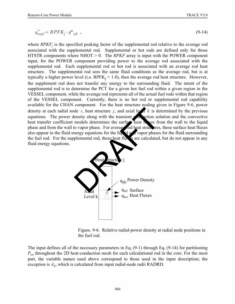
Reactor-Core Power Models TRACE V5.0
, (9-14)
where RPKFj is the specified peaking factor of the supplemental rod relative to the average rodassociated with the supplemental rod. Supplemental or hot rods are defined only for thoseHTSTR components where NHOT > 0. The RPKF array is input with the POWER componentinput, for the POWER component providing power to the average rod associated with thesupplemental rod. Each supplemental rod or hot rod is associated with an average rod heatstructure. The supplemental rod sees the same fluid conditions as the average rod, but is attypically a higher power level (i.e. RPFKj > 1.0), then the average rod heat structure. However,the supplement rod does not transfer any energy to the surrounding fluid. The intent of thesupplemental rod is to determine the PCT for a given hot fuel rod within a given region in theVESSEL component, while the average rod represents all of the actual fuel rods within that regionof the VESSEL component. Currently, there is no hot rod or supplemental rod capabilityavailable for the CHAN component. For the heat structure noding given in Figure 9-6, powerdensity at each radial node , heat structure , and axial level is determined by the previousequations. The power density along with the transient conduction solution and the convectiveheat transfer coefficient models determines the surface heat fluxes from the wall to the liquidphase and from the wall to vapor phase. For average rod heat structures, these surface heat fluxesalso appear in the fluid energy equations for the liquid and vapor phases for the fluid surroundingthe fuel rod. For the supplemental rod, these heat fluxes are calculated, but do not appear in anyfluid energy equations.
The input defines all of the necessary parameters in Eq. (9-1) through Eq. (9-14) for partitioningPtot throughout the 2D heat-conduction mesh for each calculational rod in the core. For the mostpart, the variable names used above correspond to those used in the input description; theexception is Aij, which is calculated from input radial-node radii RADRD.
Figure. 9-6. Relative radial-power density at radial node positions in the fuel rod.
qsupl''' RPFKj q'''ijk·=
i j k
Heat Structure j
AxialLevel k
iqwlqwv
qijk
SurfaceHeat Fluxes
Power DensityDRAFT
466
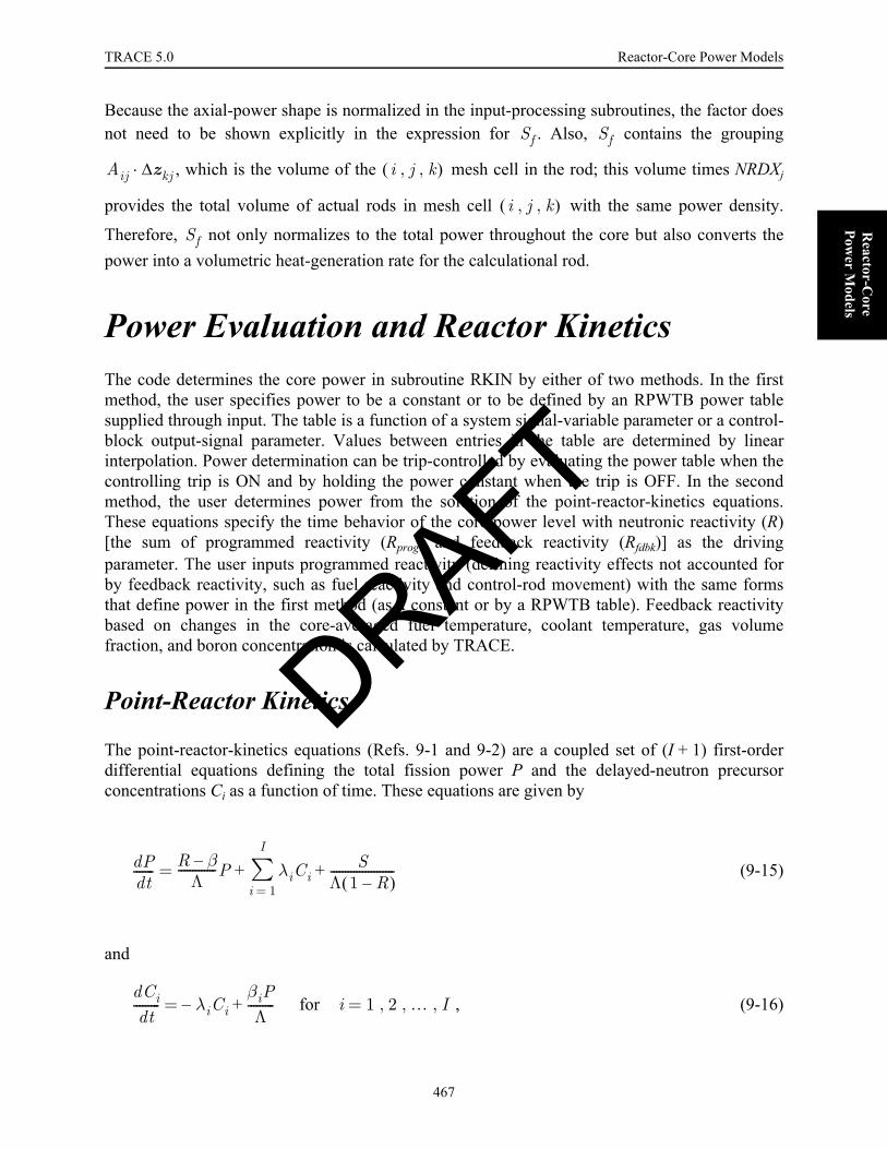
TRACE 5.0 Reactor-Core Power Models FOOBAR1234
Reactor-C
ore Pow
er Models
Because the axial-power shape is normalized in the input-processing subroutines, the factor doesnot need to be shown explicitly in the expression for . Also, contains the grouping
, which is the volume of the mesh cell in the rod; this volume times NRDXj
provides the total volume of actual rods in mesh cell with the same power density.
Therefore, not only normalizes to the total power throughout the core but also converts thepower into a volumetric heat-generation rate for the calculational rod.
Power Evaluation and Reactor KineticsThe code determines the core power in subroutine RKIN by either of two methods. In the firstmethod, the user specifies power to be a constant or to be defined by an RPWTB power tablesupplied through input. The table is a function of a system signal-variable parameter or a control-block output-signal parameter. Values between entries in the table are determined by linearinterpolation. Power determination can be trip-controlled by evaluating the power table when thecontrolling trip is ON and by holding the power constant when the trip is OFF. In the secondmethod, the user determines power from the solution of the point-reactor-kinetics equations.These equations specify the time behavior of the core power level with neutronic reactivity (R)[the sum of programmed reactivity (Rprog) and feedback reactivity (Rfdbk)] as the drivingparameter. The user inputs programmed reactivity (defining reactivity effects not accounted forby feedback reactivity, such as fuel reactivity and control-rod movement) with the same formsthat define power in the first method (as a constant or by a RPWTB table). Feedback reactivitybased on changes in the core-averaged fuel temperature, coolant temperature, gas volumefraction, and boron concentration is calculated by TRACE.
Point-Reactor Kinetics
The point-reactor-kinetics equations (Refs. 9-1 and 9-2) are a coupled set of (I + 1) first-orderdifferential equations defining the total fission power P and the delayed-neutron precursorconcentrations Ci as a function of time. These equations are given by
(9-15)
and
for , (9-16)
Sf Sf
Aij zkj∆· i j k, ,( )
i j k, ,( )
Sf
dPdt------- R β–
Λ-------------P λi
i 1=
I
∑ CiS
Λ 1 R–( )----------------------+ +=
dCidt
--------- λiCi–βiPΛ
---------+= i 1 2 … I, , ,=
DRAFT
467

Reactor-Core Power Models TRACE V5.0
where
P = thermal power (W) that results from fission occurring at time t;t = time (s);
= neutronic reactivity, k = effective neutron multiplication constant = 1 + ∆kprog + ∆kfdbk;Rprog = programmed reactivity = ∆kprog/k;Rfdbk = feedback reactivity = ∆kfdbk/k;
β = total fraction of delayed neutrons = ;
βi = fraction of delayed neutrons in group i;Λ = effective prompt-neutron lifetime (s);λi = decay constant for the delayed-neutron precursors in group i (s–1); Ci = power of the delayed-neutron precursor concentration in group i (W);I = number of delayed-neutron groups; andS = thermal power (W) from an external source of neutrons in the reactor cores that are producing fission.
The Kaganove method (Ref. 9-3) outlined in the Solution of the Point-Reactor Kinetics is used tosolve these equations.
The code applies the thermal-power solution to the decay-heat equations
for , (9-17)
where
P = solution of Eq. (9-15) and Eq. (9-16),Hj = energy of the decay-heat precursor concentration in group j (W · s),
= decay constant for decay-heat group j,Ej = effective energy fraction of decay-heat group j, andJ = number of decay-heat groups.
After solving each jth equation represented by Eq. (9-17) for the decay-heat group concentrationHj, the code calculates the total thermal power generated in the reactor-core fuel at time t. Thetotal power comprises nuclear fission, fission-product decay, and external sources as shown by
. (9-18)
R R Rprog Rfdbk+ k 1–( ) k⁄= =
βii 1=
I
∑
dHjdt
--------- λ– jHHj EjP+= j 1 2 … J, , ,=
λjH
Peff P λjHHj
j 1=
J
∑ S+ +=
DRAFT
468

TRACE 5.0 Reactor-Core Power Models FOOBAR1234
Reactor-C
ore Pow
er Models
Eq. (9-18) is consistent with the coding in TRACE version 5.0. However, Eq. (9-18) is in errorand should not include the source term S, since the contribution to reactor power associated withthe external neutron source has already been included into Eq. (9-15). This will be corrected infuture versions of TRACE. It is typical, for an external source of neutrons to be used bring a coldclean reactor up to power. Therefore, the external source term, S, would be used for a simulationfrom cold startup. The external source term is only used as part of the point-kinetics model and isnot used when the reactor power is determined from a table or a constant.
The code requires the number of delayed-neutron groups, I; the delayed-neutron parameters, λi
and βi; the number of decay-heat groups, J; the decay-heat parameters, and Ej; and either thetotal fission-power history P(t) for –t ≤ 0 or the initial delayed-neutron precursor concentrationsCi(0) and decay-heat concentrations, Hj(0).
Default Data for the Delayed-Neutron Groups
If is input (input parameter NDGX), TRACE internally sets I to 6 and defines λi and βi withthe values in Table 9-1.
If and no total fission-power history is input, the code assumes that an initial steady-statecondition exists to initialize Ci(0) internally. The code sets the time derivative in Eq. (9-16) tozero and calculates the initial values of the Ci from the following:
for , (9-19)
Table 9-1. Delayed-Neutron Constants
Group i Decay Constant λi (s–1) Neutron Fraction βi
1 3.87 0.000169
2 1.40 0.000832
3 0.311 0.00264
4 0.115 0.00122
5 0.0317 0.00138
6 0.0127 0.000247
λjH
I 0≤
I 0≤
Ci 0( )βiλiΛ---------P 0( )= i 1 2 … I, , ,=
DRAFT
469
Reactor-Core Power Models TRACE V5.0
where P(0) is the initial power specified through input. This is equivalent to assuming an infinitereactor operating period at the initial power (i.e. P(0)).
If NDGX is input > 0, then the user must supply the delayed-neutron decay constants (LAMDA)and neutron fractions (BETA). IF NDGX > 0 and NHIST = 0, then the initial values for thedelayed neutron concentrations (CDGN) must be supplied.
Default Data for the Decay-Heat Groups
If is input (i.e., J is user input for NDHX), TRACE internally sets J to the appropriate
number of decay heat groups and defines and EDj obtained from the 1979 or 1994 ANSdecay-heat standard (Refs. 9-4 and 9-5) (i.e., J may be 23, 25, 69, or 71 for the 1979 ANS decay-heat standard and J may be 92 or 94 for the 1994 ANS decay heat standard). If one of the inputoptions for the 1979 standard is used (i.e., NDHX = 69, 71, -23, or -25), the fraction of fissionpower due to each of the three isotopes, U235, Pu239, and U238, must be input. If one of the inputoptions for the 1994 standard is used (i.e., NDHX = -92 or -94), the fissionable fraction of Pu241
must also be input. In addition, in order to convert the decay energy per fission (in MeV) to afraction of the total fission energy, the energy per fission (in MeV) for each of the three or fourisotopes must be input. is converted to using the following equation:
(9-20)
where is the MeV/fission for isotope k and is the decay energy per fission per second (in
MeV/s) for decay-heat group j and is the decay constant for decay-heat group j.
If and no total fission-power history is input, the code assumes that an initial steady-state
condition exists to initialize internally. The code sets the time derivative in Eq. (9-17) to
zero and calculates the initial values of the from the following:
(9-21)
for , where P(0) is the initial steady-state power specified through input. This isequivalent to assuming an infinite reactor operating period at the initial power (i.e. P(0)).
Input requirements in the users manual describe corrections to account for fission product neutronabsorption (i.e., FISPHI and reactor operating time in power history table) and heavy element
J 0≤
λjH
EDj Ej
EjEDj
λjHQk
--------------=
Qk EDj
λjH
J 0≤
Hj 0( )
Hj
Hj 0( )Ej
λjH
-------P 0( )=
j 1 2 … J, , ,=
DRAFT
470

TRACE 5.0 Reactor-Core Power Models FOOBAR1234
Reactor-C
ore Pow
er Models
decay (i.e., NDHX = -25, 71, or 94). The user is encouraged to consult References 9-4 and 9-5 formore detailed discussions.
Fission Power History
If the total fission-power history P(–t) is input, TRACE evaluates Ci(0) and Hj(0) from Eq. (9-16)and Eq. (9-17). The P(–t) consists of tabular data pairs (tl, Pl) for l = 1, 2, . . . , L, where –tl + 1 < –t < –tl. The code assumes that the total fission power varies linearly between data pairs in thepower-history table; that is,
over the time interval . (9-22)
Substituting Eq. (8-12) into Eq. (9-16) and integrating the resulting equation analytically fromt = –tL [where Ci(–tL) = 0 is assumed] to t = 0 gives
(9-23)
One obtains a similar expression for Hj(0) by doing the same for Eq. (9-17). The expression for
Hj(0) is Eq. (9-23) with replacement of Ci by Hj, λi by , βi by Ej, and by 1. TRACEevaluates these two expressions for Ci(0) and Hj(0) when a fission-power-history table is input.
Reactivity Feedback
There are three reactivity-feedback models available in TRACE. The TRAC-P reactivity-feedback model (Ref. 9-9), the TRAC-B reactivity-feedback model (Ref. 9-10), and the RELAP5reactivity feedback model (Ref. 9-11) are all available in TRACE. The TRAC-P model isavailable when the input for TRACE is in its native input format, The TRAC-B reactivity-feedback model is used when the input is in the TRAC-B free format, and the RELAP5 reactivityfeedback model is available when the RELAP5 input model is used to generate a TRACE TPRfile via SNAP.
The TRAC-P reactivity-feedback model is based on the assumption that only changes in the core-averaged fuel temperature (Tf), coolant temperature (Tc), gas volume fraction (α), and solute mass(Bm, solute concentration in the coolant volume, or Br, ratio of solute mass to liquid-coolant massmultiplied by 1 × 10⁶) affect the neutron-multiplication reactivity of the reactor core. The code
P t( ) al blt+= tl 1+ t tl–≤ ≤–
Ci 0( ) =βiλiΛ--------- al
blλi-----–⎝ ⎠
⎛ ⎞ 1 eλi tl 1+ tl–( )–
–( )
bl tl 1+ eλi tl 1+ tl–( )–
tl–( )+
⎩
⎭
⎨
⎬
⎧
⎫eλitl–
l 1=
L 1–
∑
λjH ΛDRAFT
471

Reactor-Core Power Models TRACE V5.0
determines core-averaged values by applying a weighting factor defined as the fuel or coolantdensity times volume times power to the temperatures and solute ratio and a weighting factordefined as the volume times power to the gas volume fraction and solute concentration. Thesefactors approximate the product of the local adjoint flux, neutron flux, and volume. The (power)2
is the neutron flux times the (fission cross section)2. The neutron flux times the (fission crosssection)2 is approximating the adjoint flux. The adjoint flux is commonly called the importancefunction as applied in perturbation theory. The (fission cross section)2 makes the neutron fluxperform like the adjoint flux. This weighting-factor product, i.e., adjoint flux times neutron fluxtimes volume, is from perturbation theory where it is used to spatially weight the change inreaction-rate cross sections to estimate their reactivity change, which is consistent with one groupdiffusion theory, but not with multi-group or transport theory. TRACE approximates thisweighting-factor product by the product of the affecting-material mass (density times volume)and the fission-power density distribution raised to a user-specified power POWEXP.
The averaging process over the reactor core for the general reactivity-feedback parameter xhappens according to the following relationship:
, (9-24)
where Pi is the power, ρi is the density of the fuel or coolant and Vi is the volume of mesh cell iand the summations are over all cells in the reactor core.
For POWEXP = 1.0, the fission reaction-rate cross-section distribution approximates the adjoint-flux distribution. For POWEXP = 2.0, when the fission reaction-rate cross section is spatiallyconstant, the neutron flux approximates the adjoint flux (Galerkin approximation). Theappropriate value to use for POWEXP will depend on the fuel-loading distribution in the reactorcore. Keep in mind, however, that two levels of approximation are being made. First, it isassumed that the affecting-material density times volume times the fission-power densitydistribution raised to the POWEXP power is a good approximation for the perturbation-theoryproduct of the adjoint flux, neutron flux, and volume. Second, it is assumed that the theoreticalbasis for the use of that weighting factor for reaction-rate cross sections can be applied to thereactivity-feedback parameters that TRACE averages over the reactor core. The TRACE User’sManual suggests that POWEXP be set to 2.0 for the case where the core enrichment is radially
x
xiρiViPiPOWEXP
i∑
ρiViPiPOWEXP
i∑
-------------------------------------------------- if x is Tf Tc or Br, ,
xiViPiPOWEXP
i∑
ViPiPOWEXP
i∑
--------------------------------------------- if x is α or Bm
⎩⎪⎪⎪⎪⎪⎪⎪⎨⎪⎪⎪⎪⎪⎪⎪⎧
=
DRAFT
472

TRACE 5.0 Reactor-Core Power Models FOOBAR1234
Reactor-C
ore Pow
er Models
constant. A POWEXP=1 value may be more appropriate for the case where the radial-powerdistribution is constant across the reactor core. The user has the option of replacing any of thethree spatial shapes (fuel-rod radial, core horizontal plane, and core axial) in the fission-powerdensity distribution with a different shape to weight the spatial averaging of reactivity-feedbackparameters over the reactor core. These spatial-shape replacements are specified through input.The axial-power distribution can be input as a function of some user-defined independentvariable. For example, if that independent variable is the programmed reactivity of the controlrods, the effect of the control rods on the axial-power shape can be accounted for when the controlrods are inserted or withdrawn. An example of this is given in Volume 2 of the TRACE UsersManual.
The user defines a reactivity coefficient for each of the reactivity-feedback independent-variableparameters, x = Tf, Tc, α, and Bm or Br, by choosing one of the reactivity-coefficient forms inTable 9-2. Each reactivity coefficient is defined through input by a table of reactivity-coefficientvalues that are dependent on all four reactivity-feedback parameters. Each parameter has one ormore values specified in defining the table. Defining one value for a parameter corresponds to thereactivity coefficient having no dependence on that reactivity-feedback parameter. Defining twoor more values for a parameter gives the reactivity-coefficient dependence on one or more of thereactivity-feedback parameters. Linear interpolation is used to evaluate the reactivity coefficientfor values of each parameter between its table values. Multidimensional linear-surfaceinterpolation is performed when the reactivity coefficient is dependent on two or more of thereactivity-feedback parameters. An example of defining input data for the reactivity feedbackmodel is given in Volume 2 of the TRACE User’s Manual.
Solute in the derivative and solute dependence of a reactivity coefficient is defined in terms of thesolute concentration in the coolant channel, Bm, in units of kg/m3, a macroscopic density, or thesolute mass to liquid-coolant mass ratio, Br, in units of parts solute per million parts liquid coolant(ppm). The solute reactivity coefficient is based on the change in the amount of solute withoutchanging Tc and α when the coefficient is defined as a derivative of Br. The reactivity-coefficientderivative of Bm is affected by changes in Tc and α. Consequently, having the reactivitycoefficient as a derivative of Br is better if data are available. The solute dependence of areactivity coefficient is important when the reactivity coefficient is sensitive to a shift in theneutron-energy spectrum. Through the proportionality to the amount of neutron capture in solute,the Bm- or Br-dependence characterizes this shift. Cross-section/neutronics codes are needed todetermine this dependence separate from TRACE.
Table 9-2. Reactivity-Coefficient Forms
Form Number Reactivity-Coefficient Form
0
1
x∂∂k
1k---
x∂∂k
x∂∂R≅
DRAFT
473
Reactor-Core Power Models TRACE V5.0
All forms of solute in the reactor core are included in the evaluation of Bm or Br for solutedependence of the reactivity coefficients. Examples include dissolved boric acid in the liquidcoolant, boric acid plated on core structure, borosilicate glass in burnable-poison pins, and boronoxide in control-rod-cluster pins. The first two forms are based on boric-acid convection into thereactor core throughout the modeled system and on plate-out of boric acid in the reactor core as aresult of coolant dryout. For the latter two forms, the TRACE user defines the burnable-poison-pin and control-rod-cluster-pin forms through input with what would be their equivalent soluteconcentrations in the coolant channel. BPP or BCR define the equivalent concentration in thecoolant. A first-order-polynomial function of the core-averaged coolant temperature Tc, thecoefficients of which are input parameters, describes the equivalent burnable-poison-pin soluteconcentration as
BPP = BPP0 + BPP1 · Tc (9-25)
Whereas the physical amount of solute in the burnable-poison pins is constant during thetransient, its effective concentration for neutron capture increases with coolant temperaturebecause of reduced spatial self-shielding of solute to neutrons in those pins. The amount ofcontrol-rod-cluster-pin solute in the reactor core depends on the amount of control-rod insertioninto the core. Its effective concentration is input as a first-order-polynomial function ofprogrammed reactivity Rprog as follows:
BCR = BCR0 + BCR1 · Rprog (9-26)
Both BPP and BCR in the previous two equations have units of macroscopic solute density(kg · m–3) in the coolant-channel volume. Programmed reactivity is assumed to be proportional tothe amount of effective solute-mass change caused by control-rod movement in the core. Initially,when the reactor core is at steady-state conditions, BCR = BCR0.
Only the dissolved boric acid and that plated on solid structures in the reactor core are included inthe evaluation of Bm or Br for the solute reactivity-coefficient derivative parameter because theamount of solute in burnable-poison pins is constant during the transient that is being evaluated.Control-rod movement changes the amount of solute, but the reactivity change associated withthis movement is accounted for in the user-defined programmed reactivity Rprog. There is noreactivity feedback from control-rod movement because it is already accounted for in Rprog.
2
3
Table 9-2. Reactivity-Coefficient Forms
xx∂
∂k
xk--
x∂∂k x
x∂∂R≅
DRAFT
474
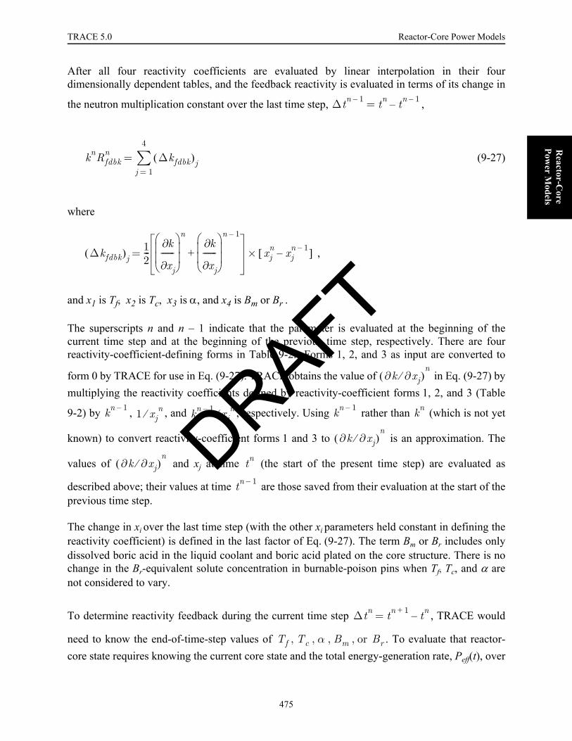
TRACE 5.0 Reactor-Core Power Models FOOBAR1234
Reactor-C
ore Pow
er Models
After all four reactivity coefficients are evaluated by linear interpolation in their fourdimensionally dependent tables, and the feedback reactivity is evaluated in terms of its change in
the neutron multiplication constant over the last time step, ,
(9-27)
where
,
and x1 is Tf, x2 is Tc, x3 is α, and x4 is Bm or Br .
The superscripts n and n – 1 indicate that the parameter is evaluated at the beginning of thecurrent time step and at the beginning of the previous time step, respectively. There are fourreactivity-coefficient-defining forms in Table 9-2. Forms 1, 2, and 3 as input are converted to
form 0 by TRACE for use in Eq. (9-27). TRACE obtains the value of in Eq. (9-27) bymultiplying the reactivity coefficients defined by reactivity-coefficient forms 1, 2, and 3 (Table
9-2) by , , and , respectively. Using rather than (which is not yet
known) to convert reactivity-coefficient forms 1 and 3 to is an approximation. The
values of and xj at time (the start of the present time step) are evaluated as
described above; their values at time are those saved from their evaluation at the start of theprevious time step.
The change in xi over the last time step (with the other xi parameters held constant in defining thereactivity coefficient) is defined in the last factor of Eq. (9-27). The term Bm or Br includes onlydissolved boric acid in the liquid coolant and boric acid plated on the core structure. There is nochange in the Br-equivalent solute concentration in burnable-poison pins when Tf, Tc, and α arenot considered to vary.
To determine reactivity feedback during the current time step , TRACE would
need to know the end-of-time-step values of . To evaluate that reactor-core state requires knowing the current core state and the total energy-generation rate, Peff(t), over
∆tn 1– tn tn 1––=
knRfdbkn ∆kfdbk( )j
j 1=
4
∑=
∆kfdbk( )j12---
k∂
x∂ j
-------⎝ ⎠⎜ ⎟⎜ ⎟⎛ ⎞ n
k∂
x∂ j
-------⎝ ⎠⎜ ⎟⎜ ⎟⎛ ⎞ n 1–
+= xjn xj
n 1––[ ]×
∂k ∂xj⁄( )n
kn 1–1 xj
n⁄ kn 1– xjn⁄ kn 1– kn
∂k ∂xj⁄( )n
∂k ∂xj⁄( )n
tn
tn 1–
∆tn tn 1+ tn–=
Tf Tc α Bm or Br, , , ,
DRAFT
475
Reactor-Core Power Models TRACE V5.0
the time step . The neutronic reactivity R(t) defined by the reactivity-feedback contribution,Rfdbk(t) must be known to determine the value of Peff(t) from the solution of the point-reactor-kinetics equations. Thus, the evaluation of reactivity feedback during the current time steprequires first knowing the time-step solution.
The TRACE code handles this difficulty of needing to know the reactivity feedback in order to
evaluate it in time step by assuming the ∆k feedback-reactivity rate is zero. The ∆kprogrammed-reactivity rate is assumed to be the same as in the previous time step, ∆tn – 1,
. (9-28)
We estimate because the input-defined independent variable needed to evaluate its tabulardefinition at tn + 1 is a function of the reactor-core state that is known at time tn. We have tested asimilar approximation for in TRAC, but near steady state it caused the sign of
to change each time step. It is better to assume that is zero than to estimate its valuebased on its value in the previous time step. Feedback effects for each time step are more tightlycoupled to than to , which causes the former estimate to be numerically unstablein some situations. Thus, estimates for the neutron-multiplication constant and neutronicreactivity for the reactor state at the end of the present time step are
(9-29)
and
(9-30)
After each time-step solution, TRACE compares the actual programmed reactivity withits estimated value. The code corrects any discrepancy by applying
(9-31)
during the next time step, . To prevent a time-step reactivity correction from becoming very
large by applying it over a time step , TRACE constrains in Eq. (9-31) to
∆tn
∆tn
∆kprogest( )
n 1+∆tn
∆kprogn
∆tn 1–-----------------
⎩ ⎭⎨ ⎬⎧ ⎫
=
kprog( )n
∆kprogest( )
n∆kfdbk
est( )n
∆kfdbkest( )
n
∆kfdbkest( )
n∆kprog
est( )n
kest( )n 1+
kn ∆kprogest( )
n 1++=
Rest( )n 1+ kest( )
n 1+1–[ ]
kest( )n 1+
-------------------------------------=
∆tn 1+
∆kcor( )n
∆kprog( )n ∆kprogest( )
n–[ ] min ∆tn 1–
∆tn----------------, 2
⎝ ⎠⎜ ⎟⎛ ⎞
·=
∆tn
tn∆ tn 1–∆ ∆kcor( )n
DRAFT
476

TRACE 5.0 Reactor-Core Power Models FOOBAR1234
Reactor-C
ore Pow
er Models
be no more than twice the time-step value. Including this correction in from the
previous time step in the neutron-multiplication constant end-of-time-step estimate at gives Eq. (9-29) in the modified form,
, (9-32)
where
.
In this procedure, we assume that and are small enough not to require an
iterative evaluation of the present time-step solution and that is large enough to beincluded in the next time-step solution rather than be neglected. The code applies a similarestimate and correction procedure to the end-of-time-step power for the case in which the totalreactor-core power is specified directly by a table.
The TRAC-B reactivity feedback model (Ref. 9-10) is based on the assumption that for BWRapplications accurate reactivity feedback cannot be obtained based on the change in core averageparameters (i.e., core average void fraction, core average moderator temperature, core averagefuel temperature, and core average boron concentration). A more accurate approximation is tosum the reactivity change for each node (i.e., fluid node for void fraction, moderator temperatureand boron concentration and fuel rod node for fuel temperature reactivity-feedback). The totalchange in reactivity is given by Eq. (9-33).
(9-33)
where,
tn 1–∆ k∆
∆tn 1+
kest( )n 1+
kn ∆kprogest( )
n 1+∆kcor( )
n+ +=
kn kn 1– ∆kprog( )n ∆kfdbk( )n+ +=
∆kcor( )n
∆kfdbk( )n 1–
∆kcor( )n
Rn Cαi αin αi
n 1––( ) WFci××i 1=
NFluid
∑
Ctmi Tlin Tli
n 1––( ) WFci 1 αin–( )×××
i 1=
NFluid
∑
Cbi Bin Bi
n 1––( ) WFci××i 1=
NFluid
∑
Ctfi Tfin( )
1 2⁄Tfi
n 1–( )1 2⁄
–⎝ ⎠⎛ ⎞ WFfi××
i 1=
NFuel
∑
+
+
+
= DRAFT
477

Reactor-Core Power Models TRACE V5.0
NFluid = Total number of fluid cells in the core, include fluid cells inside the BWR fuel assemblies, water rods, and core bypass.
NFuel = Total number of fuel nodes in the core, include all average rod groups associated with each CHAN component in the model.
= Reactivity feedback coefficient for changes in the void fraction for fluid cell i.
= Reactivity feedback coefficient for changes in the moderator temperature for
fluid cell i.
= Reactivity feedback coefficient for changes in the boron concentration for
fluid cell i.
= Reactivity feedback coefficient for changes in the fuel temperature for fuel
node i.
= Weighting factor for fluid cell i.
= Weighting factor for fuel node i.
= Void fraction in fluid cell i at time step n.
= Liquid temperature in fluid cell i at time step n.
= Boron concentration in fluid cell i at time step n.
= Fuel temperature in fuel node i at time step n.
The reactivity feedback coefficients are based on the following fits:
(9-34)
(9-35)
(9-36)
(9-37)
The RELAP5 model (Ref. 9-11) available in TRACE for RELAP5 input converted to a TRACETPR file via SNAP includes two models (i.e., a separable feedback model and a tabular feedbackmodel). The separable feedback model assumes that the reactivity feedback due to changes inmoderator density, moderator temperature, fuel temperature, and boron concentration can beseparated and are not dependent upon changes in the other reactivity feedback parameters. This
Cαi
Ctmi
Cbi
Ctfi
WFci
WFfi
αin
Tlin
Bin
Tfin
Cα Cα1 Cα2 α· Cα3 α2·+ +=
Ctm Ctm1 Ctm2 Tl· Ctm3 Tl2·+ +=
Ctf Ctf1 Ctf2 α· Ctf3 α2·+ +=
Cb Cb1 Cb2 B· Cb3 B2·+ +=
DRAFT
478

TRACE 5.0 Reactor-Core Power Models FOOBAR1234
Reactor-C
ore Pow
er Models
assumption is typically valid for reactor core close to critical and with relatively small boronconcentrations. The tabular feedback model assumes that there are interactions between thedifferent reactivity feedback effects, which cannot be neglected. For example during an ATWS,the reactivity feedback due to moderator density may be a function of the boron concentration,moderator temperature, and/or fuel temperature.
The reactivity feedback for the separable feedback model can be written as:
(9-38)
where,nScram = Number of general table scram curves.
nControl = Number of signal variables/control blocks used to specify programmed or reactivity feedback.
= Reactivity associated general table scram curves at time step n.
= Reactivity associated signal variable/control blocks.
= Moderator density reactivity feedback table as a function of core average
moderator density.
= Fuel temperature reactivity feedback table as a function of fuel temperature.
= Moderater temperature reactivity feedback table as a function of moderator
temperature.
= Boron solute reactivity feedback table as a function of boron concentration.
The reactivity feedback model for the tabular feedback is given as:
(9-39)
where is the total reactivity table for a given fuel temperature, moderatordensity, moderator temperature, and boron concentration.
For the separable and tabular reactivity feedback models, the moderator density may be replacedwith void fraction, depending upon the RELAP5 options selected in the original RELAP5 inputmodel. The RELAP5 options for reactivity feedback have not been fully tested and should beused with caution. Note that currently the RELAP5 options for reactivity feedback are onlyavailable if the RELAP5 input was converted to a TRACE TPR file via SNAP. The capability to
Rn Rnsi
i 1=
nScram
∑ Rnci
i 1=
nControl
∑ Rρ ρmn( ) Rf TF
n( ) RB Bn( ) Rm Tmn( )+ + + + +=
Rnsi
Rnci
Rρ ρm( )
RF TF( )
Rm TM( )
RB B( )
Rn RT TFn ρm
n Tmn B,
n, ,( )=
RT TFn ρm
n Tmn B, c
n, ,( )
DRAFT
479

Reactor-Core Power Models TRACE V5.0
access these models via TRACE ASCII input will be provided in future versions of TRACE asdetermined by user needs.
Solution of the Point-Reactor Kinetics
The code solves the point-reactor-kinetics equations Eq. (9-15) through Eq. (9-17) by theKaganove method (Ref. 9-3). Its derivation approximates the time dependence of P and
over each integration time step by second-order polynomials and
assumes where is a constant. For TRACE, it is more appropriate toapproximate the time dependence of P by a second-order polynomial, R by a first-orderpolynomial, and Λ by a constant because TRACE linearly extrapolates its estimate of overthe fluid-dynamics time step to be evaluated and because the weak time dependence of Λgenerally is unknown. These modified assumptions, when applied to the point-reactor-kineticsequations, simplify the form that these equations take when analytically integrated over theneutronics integration time step ∆t. The derivation of those analytically integrated equations is
given below. TRACE then evaluates them for integration time steps during the fluid-dynamics time step.
In TRACE, the neutronics solution is solved before the hydraulic and heat-conduction solutions.Otherwise, the linear extrapolation estimates in the previous sub-section would not have to bedone if the hydraulic and heat-conduction solutions were solved first. The heat-conductionsolution would be more implicit if it were done after the neutronics solution. Another order wouldbe to do the hydraulics solution first, the neutronics solution next, and then the heat-conductionsolution.
We assume
(9-40)
(9-41)
where , , and are all known values, and that
are constant over the interval ,
Solving Eq. (9-16) for in terms of a functional of the fission power gives
kex k 1– R 1 R–( )⁄= =
Λ t( ) 1 kex t( )+( )⁄=
R t( )
∆tn ∆t⁄ ∆tn
P t( ) P 0( ) P1t P2t2+ +=
R t( ) R 0( ) R1t+=
P 0( ) R 0( ) R1 Rest( )n
R 0( )–[ ] ∆tn⁄=
Λ λi βi λjH and Ej,,,, 0 t ∆t≤ ≤
Ci t( ) P t( )
DRAFT
480

TRACE 5.0 Reactor-Core Power Models FOOBAR1234
Reactor-C
ore Pow
er Models
(9-42)
Substituting Eq. (9-42) into Eq. (8-6) and integrating the resulting equation term-by-term gives
(9-43)
Note that Eq. (9-43) assumes R1 is not equal to zero. If R1 is zero, then the last term in Eq. (9-43)
is . Substituting Eq. (9-33) for and Eq. (9-41) for in Eq. (9-43),
evaluating the integrals, and rearranging the resulting equation in terms of the and unknowns gives
(9-44)
where
(9-45)
(9-46)
Ci t( ) Ci 0( )eλit– βi
Λ----- e
λi t τ–( )–P τ( ) τd
0
t
∫+=
P t( ) P 0( ) R τ( )P τ( )Λ
------------------------- τd0
t
∫ βiΛ----- e
λi t τ–( )–P τ( ) τd
0
t
∫i 1=
I
∑–+=
Ci 0( ) 1 eλit–
–[ ] SΛR1----------- 1 R 0( )–
1 R 0( )– R1t–------------------------------------ln+
i 1=
I
∑
+
StΛ 1 R 0( )–( )------------------------------ P τ( ) R τ( )
P1 P2
a1 t( )P1 a2 t( )P2+ q t( )=
a1 t( ) tΛ t2 12---R 0( ) 1
3---R1t+ βit
2Ii1 t( )i 1=
I
∑+–=
a2 t( ) t2Λ t3 13---R 0( ) 1
4---R1t+ βit
3Ii2 t( )i 1=
I
∑+–=
DRAFT
481

Reactor-Core Power Models TRACE V5.0
(9-47)
or if R1 is zero
(9-48)
and
(9-49)
Note the coding in TRACE is currently in error in that the source term in Eq. (9-47) appears as:
(9-50)
This will be corrected in a future version of TRACE.
The and polynomial coefficients are evaluated by requiring Eq. (9-44) to be satisfied for
(at the end of the integration time step) and (at the midpoint of the integrationtime step). Solving the two equations
q t( ) SR1------ 1 R 0( )–
1 R 0( )– R1t–------------------------------------ln t R 0( ) 1
2---R1t+ P 0( )
ΛλiCi 0( ) βiP 0( )–[ ]tIi0 t( )i 1=
I
∑
+ +=
q t( ) St1 R 0( )–--------------------- tR 0( )P 0( ) ΛλiCi 0( ) βiP 0( )–[ ]tIi0 t( )
i 1=
I
∑+ +=
Iim t( )
e λ t τ–( )– τm τd0
t
∫
tm 1+-------------------------------------- for m 0, 1, 2= =
q t( ) S 1 R 0( )t– 12---R1t
2– t R 0( ) 12---R1t+ P 0( )
ΛλiCi 0( ) βiP 0( )–[ ]tIi0 t( )i 1=
I
∑
+ +=
P1 P2
t ∆t= t ∆t 2⁄=
DRAFT
482
TRACE 5.0 Reactor-Core Power Models FOOBAR1234
Reactor-C
ore Pow
er Models
(9-51)
and
(9-52)
for and gives
(9-53)
and
(9-54)
where
.
The total fission power at the end of the integration time step from Eq. (9-40) is
. (9-55)
If we know for we can evaluate by substituting Eq. (9-40) intoEq. (9-42) and using
(9-56)
(9-57)
by analytically integrating its definition in Eq. (9-44) as follows:
a1 ∆t( )P1 a2 ∆t( )P2+ q ∆t( )=
a1∆t2
-------⎝ ⎠⎛ ⎞ P1 a2
∆t2
-------⎝ ⎠⎛ ⎞ P2+ q ∆t
2-------⎝ ⎠
⎛ ⎞=
P1 P2
P1
q ∆t( )a2∆t2
-------⎝ ⎠⎛ ⎞ q ∆t
2-------⎝ ⎠
⎛ ⎞ a2 ∆t( )–
D--------------------------------------------------------------------------------=
P2
a1 ∆t( )q ∆t2
-------⎝ ⎠⎛ ⎞ a1
∆t2
-------⎝ ⎠⎛ ⎞ q ∆t( )–
D--------------------------------------------------------------------------------=
D a1 ∆t( )a2∆t2
-------⎝ ⎠⎛ ⎞ a1
∆t2
-------⎝ ⎠⎛ ⎞ a2 ∆t( )–=
t ∆t=
P ∆t( ) P 0( ) P1∆t P2∆t2+ +=
P t( ) 0 t ∆t≤ ≤ Ci ∆t( )
∆tIi0 ∆t( ) 1 eλi∆t–
–λi
-----------------------=
∆tm 1+ Iim ∆t( )∆tm m∆tmIim 1– ∆t( )–
λi------------------------------------------------------------- for m 1, 2= =
DRAFT
483
Reactor-Core Power Models TRACE V5.0
(9-58)
for i = 1, 2, . . . , I.
The code evaluates the decay-heat equations in the same way to give
(9-59)
for j = 1, 2, . . . , J, and where
. (9-60)
The code evaluates with the following recursion relation:
(9-61)
once
is first evaluated. For , Eq. (9-61) results in the loss of several least-significant digits of
accuracy with each application of the recursion formula. Thus, for , TRACE first
evaluates using the Maclaurin expansion,
Ci ∆t( ) Ci 0( ) 1 λi∆tIi0 ∆t( )–[ ]
βiΛ----- P 0( )∆tIi0 ∆t( ) P1∆t2Ii1 ∆t( ) P2∆t3Ii2 ∆t( )+ +
+=
Hj ∆t( ) Hj 0( ) 1 λjH∆tIj0
H ∆t( )–[ ]
Ej P 0( )∆tIj0H ∆t( ) P1∆t2Ij1
H ∆t( ) P2∆t3Ij2H ∆t( )+ +
+=
∆tm 1+ IjmH ∆t( ) e
λjH ∆t τ–( )– τm τd
0
∆t
∫=
∆tm 1+ Iim ∆t( )
∆tm 1+ IjmH ∆t( )
∆tm m∆tmIjm 1–H ∆t( )–
λjH
------------------------------------------------------------- for m 1, 2= =
∆tIi0H ∆t( ) 1 e
λjH∆t–
–λj
H-------------------------=
λi∆t 1<
λi∆t 1<
∆t3Ii2 ∆t( )
DRAFT
484

TRACE 5.0 Reactor-Core Power Models FOOBAR1234
Reactor-C
ore Pow
er Models
(9-62)
for m = 2, and then evaluates the reciprocal of the Eq. (9-59),
(9-63)
A maximum of the first 13 terms in the series expansion for Eq. (9-62) is included if .The sum is terminated if the absolute value of the next term in the series divided by the sum of all
previous terms is less than 10-14. For , the analytical solution given by Eq. (9-61) isused.
The accuracy of the second-order polynomial approximation for P(t) can be increased bydecreasing the integration time-step size ∆t. We would like ∆t to be as large as possible, however,while we maintain a desired level of accuracy in approximating P(t). To achieve this, thefollowing procedure for automatically adjusting the reactor-kinetics time step in TRACE is used.In the same manner that Eq. (9-51) and Eq. (9-52) were defined, Eq. (9-43) also could be required
to be satisfied at by
. (9-64)
The above equation together with Eq. (9-52), which is evaluated at , are solved over the
time range for and to give
(9-65)
and
(9-66)
where
∆tm 1+ Iim ∆t( ) ∆tm 1+ m! 1m 1+( )!
---------------------λi∆tm 2+( )!
---------------------λi∆t( )2
m 3+( )!--------------------- . . .–+–=
∆tmIim 1– ∆t( )∆tm λ∆tm 1+ Iim ∆t( )–
m------------------------------------------------------------ for m 2, 1= =
λi∆t 1<
λi∆t 1≥
t ∆t 4⁄=
a1∆t4
-------⎝ ⎠⎛ ⎞ P1 a2
∆t4
-------⎝ ⎠⎛ ⎞ P2+ q ∆t
4-------⎝ ⎠
⎛ ⎞=
t ∆t 2⁄=
0 t ∆t 2⁄≤ ≤ P1 P1∗= P2 P2∗=
P1∗q ∆t
2-------⎝ ⎠
⎛ ⎞ a2∆t4
-------⎝ ⎠⎛ ⎞ q ∆t
4-------⎝ ⎠
⎛ ⎞ a2∆t2
-------⎝ ⎠⎛ ⎞–
D∗----------------------------------------------------------------------------=
P2∗q ∆t
4-------⎝ ⎠
⎛ ⎞ a1∆t2
-------⎝ ⎠⎛ ⎞ q ∆t
2-------⎝ ⎠
⎛ ⎞ a1∆t4
-------⎝ ⎠⎛ ⎞–
D∗----------------------------------------------------------------------------=
DRAFT
485
Reactor-Core Power Models TRACE V5.0
This solution over half the integration time step provides a more accurate value for at
,
(9-67)
than the solution over the full integration time step at ,
(9-68)
The code uses the difference between these two values as a measure of the error in the solutionover the full integration time step
(9-69)
It is desirable to increase if the above ε is too small and to decrease if ε is too large.Toward this end, the code defines two error bounds, and , to provide the desiredconvergence such that,
1) if , the code maintains the present value of reactor-kinetics time step
;
2) if , the code halves the value of because the error in is too large; and
3) if , the code doubles the value of because the error in is too small.
When is halved, the integration time step is reevaluated. When the third criterion is satisfied,the number of remaining integration time steps to be evaluated over the fluid-dynamics time stepmust be an even number for the integration time step to be doubled (and the number of remainingintegration time steps to be halved). TRACE is programmed to use ε1 = 10−6 and ε2 = 10−4. Anumerical study showed these values to yield a maximum fractional error less than 10−4 and an
D∗ a1∆t2
-------⎝ ⎠⎛ ⎞ a2
∆t4
-------⎝ ⎠⎛ ⎞ a2
∆t2
-------⎝ ⎠⎛ ⎞ a1
∆t4
-------⎝ ⎠⎛ ⎞–=
P t( )
t ∆t 2⁄=
P∗ ∆t2
-------⎝ ⎠⎛ ⎞ P 0( ) P1∗ ∆t
2-------⎝ ⎠
⎛ ⎞ P2∗ ∆t2
-------⎝ ⎠⎛ ⎞ 2
+ +=
t ∆t 2⁄=
P ∆t2
-------⎝ ⎠⎛ ⎞ P 0( ) P1
∆t2
-------⎝ ⎠⎛ ⎞ P2
∆t2
-------⎝ ⎠⎛ ⎞ 2
+ +=
∆t
ε ∆t( )P ∆t
2-------⎝ ⎠
⎛ ⎞ P∗ ∆t2
-------⎝ ⎠⎛ ⎞–
P∗ ∆t2
-------⎝ ⎠⎛ ⎞
-------------------------------------------=
∆t ∆tε1 ε2
ε1 ε ∆t( ) ε2< <
∆t
ε1 ε2 ε ∆t( )≤< ∆t P ∆t( )
ε ∆t( ) ε≤ 1 ε2< ∆t P ∆t( )
∆t
DRAFT
486

TRACE 5.0 Reactor-Core Power Models FOOBAR1234
Reactor-C
ore Pow
er Models
average fractional error less than 10−5 in the fission power solution. The point-reactor-kineticssolution required < 1% of TRACE execution time.
Conclusions Regarding the Reactor-Core Power ModelThe core-power model in TRACE, with all the options and features, has proved to be sufficientlygeneral for describing core assemblies in most reactor-safety-related experiments, particularlyones that are integral in nature, and in reactor plants, provided that the power shape only changesin time in the axial direction. For this to be true, the axial-power shape must be specified as afunction of some user-defined independent variable for the axial-power-shape table. The option tospecify core power directly with a tabular prescription is generally sufficient for modeling mosttransients of interest where the power-level behavior is known.
The point-reactor kinetics with reactivity feedback model has demonstrated (for many cases ofthe TRACE developmental assessment problem set) the ability to describe the transient powerresponse of a reactor core. For example, in the case of anticipated transients without scram, thecore-power behavior would not be known because of reactivity-feedback effects, and in this case,reactor kinetics is a necessary capability. In analyzing experiments from the LOFT facility (forexample, the L6-1 test simulating a loss-of-steam-load transient) and transients from power plants(for example, the Zion PWR standard test problem), reactor kinetics has demonstrated a goodpredictive capability. For performing best-estimate analyses of large-break LOCAs, reactorkinetics has demonstrated the ability to predict the shutdown of core power by core voidingbefore the control-rod scram is effective.
For a specific reactor transient where multi-dimensional transient neutronics is important,TRACE coupled with PARCS can be used for this simulation (i.e. BWR stability transients).However, for a number of accident scenarios, point-kinetics or specified is power is sufficient.
The decay heat models available in TRACE can be used to accurately simulate the decay heatpower levels associated with a nuclear reactor and determine the amount of decay heat for a givenreactor power history. The user has the option to use a few group decay heat model with aminimum of user input, which will give approximate results or as many as 92 decay heat groupsconsistent with the 1994 decay heat standard. The decay power levels can be based on a specifiedreactor operating history or infinite operation at the initial power level and is calculated consistentwith the decay heat model selected by the user.
The deficiencies of the core-power model are principally related to the fact that reactor kinetics isbased on a point-reactor assumption, and the power distribution is defined by a superposition offuel-rod-radial, core-axial, and (r, θ)-plane shapes. Axial-shape changes in the power distributionwith a known dependence can be simulated, but fuel-rod-radial and core (r, θ)-plane power-shapechanges and power distributions that are not definable by superimposed fuel-rod-radial, core-axial, and (r, θ)-plane shapes cannot be modeled. Reactivity feedback is also based on the point-
DRAFT
487

Reactor-Core Power Models TRACE V5.0
reactor assumption with little theoretical justification for the procedure used to core average thereactivity-feedback parameters. Asymmetric and localized reactivity-feedback effects andcontrol-rod movements in the reactor core cannot be modeled accurately. However, within thesemodeling limitations, the core-power model is accurate and efficient in determining the time-dependent behavior of the reactor-core power. To further assess the point-kinetics model requireshaving good core neutronics data (power shape, reactivity coefficients, etc.) and use of neutronicscodes to generate the point-kinetics input data.
For transients in which 3D neutronics effects are important (i.e., BWR instabilities), TRACE canbe coupled to the PARCS. When TRACE is coupled to PARCS a POWER component is stillrequired in the TRACE model to ensure that necessary power density arrays have been allocatedso that the PARCS transient 3D power can be loaded into the appropriate array element locationsin TRACE.
References9-1 Reactor Physics Constants,” Argonne National Laboratory report ANL-5800, 2nd ed.
(July 1963).
9-2 A. Rodkowsky, Ed., “Naval Reactors Physics Handbook, Vol. 1: Selected BasicTechniques,” Library of Congress Number 65-60008 (1964).
9-3 J. J. Kaganove, “Numerical Solution of the One-Group Space-Independent ReactorKinetics Equations for Neutron Density Given the Excess Reactivity,” Argonne NationalLaboratory report ANL-6132 (1960).
9-4 American National Standard for Decay Heat Power in Light Water Reactors,” AmericanNuclear Society publication ANSI/ANS-5.1 (1979).
9-5 American National Standard for Decay Heat Power in Light Water Reactors,” AmericanNuclear Society publication ANSI/ANS-5.1 (1994).
9-6 TRACE Users Manual.
9-7 Joe, H.C., Barber, D., Jiang, G., and Downar, T. J., "PARCS, A Multi-Dimensional Two-Group Reactor Kinetics Code Based on the Nonlinear Analytic Nodal Method," PU/NE-98-26, Sept. 1998.
9-8 Volume 2: User Manual for the PARCS Kinetic Core Simulator Module.
9-9 J. W. Spore, et.al., "TRAC-M/FORTRAN 90 Version 3.0 Theory Manual," NUREG/CR-6724, July, 2001.
DRAFT
488

TRACE 5.0 Reactor-Core Power Models FOOBAR1234
Reactor-C
ore Pow
er Models
9-10 M. M. Giles, et. al., "TRAC-BF1/MOD1: An Advanced Best Estimate Computer Programfor Boiling Water Reactor Accident Analysis, Volume I: Model Description," May 1992,INEL.
9-11 RELAP5/MOD3.3 Code Manual Volume I: Code Structure, System Models, and SolutionMethods," NSAD, December, 2001, ISL, Rockville, Maryland, Idaho Falls, ID
DRAFT
489

Reactor-Core Power Models TRACE V5.0
DRAFT
490

TRACE V5.0 Special Component Models FOOBAR1234FOOBAR1234
Special C
omponent
Models
10 Special Component Models
FOOBAR1234FOOBAR1234FOOBAR1234
Some one-dimensional components in TRACE perform special functions that requiremodification of the solution of the 1D fluid equations. These modifications are more than simplyaltering the normal closure relations that have been discussed in previous chapters; thesecomponents either alter the normal finite differencing of the fluid equations, introduce sourceterms to the equations, or use complex logic to alter the closure relations to accomplish a specificmodeling requirement. The PUMP component produces a momentum source term in the form ofan additional ∆P on the right-hand side of the momentum equation to model the pressure riseacross the pump impeller. The PRIZER component models a PWR pressurizer. The steam/waterseparator/dryer component (SEPD) permits the user to model the swirl separators and chevrondryers in a BWR reactor. The JETP component models the jet pumps found in BWR systems byuse of the TEE component momentum source in the TEE joining cell and jet pump specificsingular loss coefficients.
Nomenclature = area ratio of outlet to inlet flow area for the jet pump
= swirl vane flow area in separator
= standpipe flow area in separator
= contraction constant for the jet pump
= expansion constant for the jet pump
= friction coefficient
= total loss coefficient in the discharge passage of the separator
= contraction loss coefficient
= critical dryer inlet moisture
= carry-over ratio
A∗
An
Ai
Cc
Ce
Cf
CK
CNOZ
CDIM
CO
DRAFT
491

Special Component Models TRACE V5.0
= carry-under ratio
= specific heat at constant pressure
= hydraulic diameter in the discharge passage of the separator
= range of inlet moisture over which the dryer capacity goes from one to zero for a fixed vapor inlet velocity
= dryer inlet moisture
= effective L/D coefficient at the separator pick-off ring
= axial component of frictional force on swirling water later
= resultant frictional force
= tangential component of frictional force on swirling water layer
= gravitational acceleration
= SEPD capacity factor
= normalized pump head
= normalized pump head from the single-phase performance curve
= normalized pump head from the two-phase fully degraded performance curve
= pump head
= rated pump head
= single-phase pump head
= two-phase fully-degraded pump head
= axial distance between the separator hub and the bottom of the discharge
passage
= length of separator barrel
= height of the liquid pool surrounding the separator relative to the bottom of the
discharge passage
= pump moment of inertiajcell = cell index on the primary side of a TEE component, where the secondary side
is connected to the primary side.
= contraction irreversible loss factor for the jet pump
= expansion irreversible loss factor for the jet pump
= total liquid mass in the PRIZER
CU
cp
DD
DELDIM
DIM
EFFLD
Fa
Ff
Ft
g
GDRY
h
h1φ
h2φ
H
HR
H1φ
H2φ
Hsk
HD
H12
I
Kc
Ke
LMT
DRAFT
492

TRACE V5.0 Special Component Models FOOBAR1234FOOBAR1234
Special C
omponent
Models
= mass flow rate
= ratio of liquid mass flow rate in the drive nozzle of the jet pump to liquid mass flow rate in the suction of the jet pump
= pump head degradation multiplier
= ratio of specific energy increase in the suctio flow to the specific energy decrease in the drive nozzle flow
= pump torque degradation multiplier
= TRACE calculated pressure in cell 1 of the PRIZER
= user-supplied pressure offset at which heater/sprays achieve maximum
effectiveness
= pressure in the vapor core of the separator
= user-supplied pressure setpoint for the PRIZER
= pressure at the separator wall
= normalized pump volumetric flow
= heat generated by pump due to friction
= pump volumetric flow
= energy added/removed from liquid in an individual PRIZER cell
= user-supplied maximum effective power of the PRIZER heater/sprays
= energy added/removed from the PRIZER
= rated pump volumetric flow
= radius
= inner radius of the water layer in the separator
= radius of the separator barrel
= radius of the separator pick-off ring
= liquid Reynolds number
= slip ratio
= pump momentum source term
= time
= pump hydraulic torque acting on the impeller
m·
M
M α( )
N
N α( )
P1
∆Pmax
Po
Pset
Pw
q
qfric
Q
Qf
Qheat
Qin
QR
r
rf
rw
rr
REL
S
Smom
t
T
DRAFT
493

Special Component Models TRACE V5.0
= pump friction torque acting on the rotating parts of the motor
= hydraulic torque
= rated pump torque
= velocity
= axial velocity
= axial velocity in the water layer
= axial velocity in the vapor core
= axial velocity at the swirl vane
= velocity in the discharge passage
= tangential velocity
= tangential velocity at the swirl vane
= tangential velocity on the wall
= resultant swirling velocity on the wall
= vapor velocity below which any amount of moisture is assumed to be separated from the vapor stream
= vapor velocity above which no amount of moisture, however small, can be separated from the vapor stream
= volume
= total liquid volume in the pressurizer
= mass flow rate
= total flow rate
= total discharge flow
= cell length
or = quality
= inlet flow quality
= collapsed liquid level
= void fraction or angle of the jet pump diffuser
= normalized pump hydraulic torque
= normalized pump hydraulic torque from single phase torque curves
Tf
Thy
TR
V
Va
Vaf
Vag
Van
VD
Vt
Vtn
Vtw
Vw
VDRY1
VDRY2
Vol
Volliq
W
Wi
WD
∆x
x X
Xi
XL
α
β
β1φ
DRAFT
494
TRACE V5.0 Special Component Models FOOBAR1234FOOBAR1234
Special C
omponent
Models
= normalized pump hydraulic torque from two phase fully-degraded torque
curves
= density
= mean density
= normalized pump speed
= pump speed (impeller angular velocity)
= rated pump speed
= angle between swirl vanes and the horizontal plane
Subscripts
= denotes a liquid carry-over quantity
= denotes a vapor carry-under quantity
= applies to the discharge arm of the SEPD
= denotes a donor-cell (upstream) quantity
= denotes the drive nozzle of a jet pump
= denotes the discharge of a jet pump
= applies to the exit of the SEPD
or = denotes a liquid quantity
= denotes a gas phase quantity
= denotes a hydraulic quantity
= applies to the inlet of the SEPD
= denotes a quantity that applies to the cell center
= denotes a quantity that applies to a cell edge (center of a momentum cell)
= denotes a quantity that applies to the downstream cell
= index of cell in PRIZER that contains the collapsed liquid level
= denotes a mixture quantity
= denotes the suction line of a jet pump
Superscripts
= denotes an old-time level quantity
= denotes a current or new-time level quantity
β2φ
ρ
ρ
ω
Ω
ΩR
θ
CO
CU
DIS
donor
d
ds
EX
f l
g
hy
IN
j
j 1 2⁄+
j 1+
k
m
s
n
n 1+
DRAFT
495

Special Component Models TRACE V5.0
PUMP ComponentThe PUMP component describes the interaction of the system fluid with a centrifugal pump. Itcalculates the pressure differential across the pump impeller and the pump impeller's angularvelocity as a function of the fluid flow rate and fluid properties. The model can simulate anycentrifugal pump and allows for the inclusion of two-phase effects.
The following considerations were made in creating the PUMP component:
1) compatibility with adjacent components should be maximized,
2) choking at the pump-impeller interface should be predicted automatically by the pump-curve data, and
3) the calculated pressure rise across the pump-impeller interface should agree with that measured at steady-state conditions.
The first two criteria preclude the use of a lumped-parameter model. Instead, the PUMPcomponent has been implemented as a variant of the PIPE component, but with pump-curvecorrelations that define an extra momentum source at the pump-impeller interface. At its heart,the PUMP component is really nothing more than a means of specifying a cell edge that shouldact like the impeller in a pump, imparting momentum to the fluid around it.
Pump Governing Equations
While the User Guide presents several possible PUMP component representations, Figure 10-1illustrates a generic way of conceptualizing the pump model. It shows two mesh cells, labeled and , that straddle the pump impeller interface (labeled with index ). Superimposedover that is the momentum cell over which the motion equations for the interface are solved(denoted by the dashed box). When modeled in the traditional manner1, (i.e. the PUMP has twoor more cells), cells and correspond to cells 1 and 2, respectively. However, because aPUMP component can be modeled as a single face with zero cells, cells and may actuallybelong to other 1D components.
The PUMP-component model is identical to the 1D PIPE-component model except that themotion equations for the interface between cells and are approximated by
1. In the legacy model inherited from TRAC-P, PUMP components must have two or more computational cells, with the pump-impeller interface hardwired to exist at the second face. The ability to model a PUMP as a single cell face with zero cells was added later, as part of the NRC’s code consolidation project (to recapture some of RELAP5’s capabilities). It is not possible to define a PUMP component with just one mesh cell.
j
j 1+ j 1 2⁄+
j j 1+j j 1+
j j 1+
DRAFT
496

TRACE V5.0 Special Component Models FOOBAR1234FOOBAR1234
Special C
omponent
Models
(10-1)
and
, (10-2)
where is the length of the momentum cell, is the mean mixture density of
the momentum cell, and is the first-order approximated pressure rise momentum sourceacross the pump-impeller interface evaluated from the pump-curve correlations. It is given by thefollowing expression:
(10-3)
The pressure rise, , and its derivative with respect to the coolant velocity, , for the
pump-impeller interface is evaluated only once at the beginning of each timestep. Thismomentum source is applied in the coolant motion equation at the pump-impeller interface. Themean mixture density is calculated from the following relationship:
Figure. 10-1. Generic PUMP model conceptualization.
j j+1j+1/2
Pump ImpellerInterface
Pj+1Pj
j+1
j+1
xj+1/2
Smom
Vg
j
j
Vl
Vgn 1+ Vg
n–∆t
---------------------------Pj
n 1+ Pj 1+n 1+– Smom
n 1++[ ]
ρm( )j 1 2⁄+n
∆xj 1 2⁄+·---------------------------------------------------------- g θcos·–=
Vln 1+ Vg
n 1+=
∆xj 1 2⁄+ρm( )j 1 2⁄+
Smom
Smomn 1+ ∆Pn ∂∆P
∂V-------------⎝ ⎠
⎛ ⎞ nVg
n 1+ Vgn–( )·+
⎩ ⎭⎨ ⎬⎧ ⎫
=
∆Pn ∂∆P∂V
-------------⎝ ⎠⎛ ⎞ n
DRAFT
497

Special Component Models TRACE V5.0
(10-4)
where is a donor-cell evaluated void fraction. Given that the phasic densities are knownat the cell-center, the mean phasic densities at the cell edge are calculated using a cell-lengthweighting procedure, as given by:
(10-5)
(10-6)
where and represent the cell lengths of the and cells, respectively. In all of
the above equations, the and superscripts indicate that quantities should be evaluated atthe old-time and new-time levels, respectively.
Friction and form losses do not enter explicitly into Eq. (10-1) because we assume that the frictioneffects are normally included in the homologous curves defining the pump head. Therefore, walldrag and additive friction losses are not modeled between the centers of cells and .
During a steady state, the pressure rise across the pump can be determined by recognizing that thevelocity difference terms in Eq. (10-1) become zero, giving rise to the following equation:
, (10-7)
The time level superscripts have been eliminated as they are irrelevant for a steady state.
Pump Head Modeling
The pump modeling in TRACE is based on the standard homologous-curves approach. Thesecurves represent the performance of the pump in a normalized format, giving the normalizedpump head as a function of the normalized volumetric flow and normalized pump speed.Homologous curves (one curve segment represents a family of curves) are used for thisdescription because of their simplicity. These curves describe, in a compact manner, all operatingstates of the pump obtained by combining positive or negative pump-impeller angular velocitieswith positive or negative fluid volumetric flows. While TRACE maintains several sets of built-incurves for some well-used pump types, you are also offered the option of supplying your own.
The following definitions are used in the subsequent development:
ρm( )j 1 2⁄+n
αdonorρ g( )j 1 2⁄+
n1 αdonor–( ) ρ l( )j 1 2⁄+
n+=
αdonor
ρ g( )j 1 2⁄+n ∆xj
ρg( )jn ∆xj 1+ ρg( )j 1+
n+∆xj ∆xj 1++
----------------------------------------------------------------------=
ρ l( )j 1 2⁄+n ∆xj
ρl( )jn ∆xj 1+ ρl( )j 1+
n+∆xj ∆xj 1++
--------------------------------------------------------------------=
∆xj ∆xj 1+ j j 1+
n n 1+
j j 1+
∆P Pj 1+ Pj– ρm( )j 1 2⁄+ ∆xj 1 2⁄+ g θcos· ··+= DRAFT
498

TRACE V5.0 Special Component Models FOOBAR1234FOOBAR1234
Special C
omponent
Models
= the pump head, (Pa-m3/kg, m2/s2, or N-m/kg),
= the impeller-interface volumetric flow rate, (m3/s), and
= the pump-impeller angular velocity (rad/s),
where is the pressure rise across the pump-impeller interface and is the impeller-interface upstream coolant-mixture density. To allow one set of curves to be used for a variety ofpumps, the following normalized quantities are used:
(10-8)
(10-9)
(10-10)
where is the rated head, is the rated volumetric flow, and is the rated pump-impeller
rotational speed for the pump1. The pump similarity relations (Ref. 10-2) show that
(10-11)
For small , this correlation is not satisfactory, so the following combination of variables is used,
. (10-12)
Eq. (10-11) is used in the range and results in two separate curves, one for
and one for . Eq. (10-12) is used in the range and yields two separate
curves, one for and one for . The four resulting curve segments, as well as the curveselection criteria used in TRACE, are shown in Table 10-1.
1. The rated quantities are provided through input
H ∆P( ) ρm⁄
Q Aj 1 2⁄+
Vj 1 2⁄+
·
Ω
∆P ρm
h H HR⁄=
q Q QR⁄=
ω Ω ΩR⁄=
HR QR ΩR
h ω2⁄ f q ω⁄( )=
ω
h q2⁄ f ω q⁄( )=
0 q ω⁄ 1≤ ≤ ω 0>
ω 0< 0 ω q⁄ 1≤ ≤
q 0> q 0<
DRAFT
499
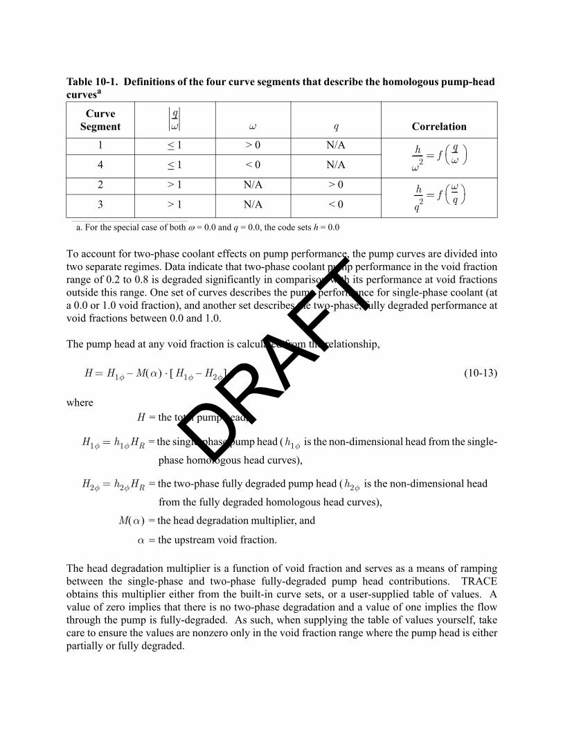
To account for two-phase coolant effects on pump performance, the pump curves are divided intotwo separate regimes. Data indicate that two-phase coolant pump performance in the void fractionrange of 0.2 to 0.8 is degraded significantly in comparison with its performance at void fractionsoutside this range. One set of curves describes the pump performance for single-phase coolant (ata 0.0 or 1.0 void fraction), and another set describes the two-phase, fully degraded performance atvoid fractions between 0.0 and 1.0.
The pump head at any void fraction is calculated from the relationship,
, (10-13)
where = the total pump head,
= the single-phase pump head ( is the non-dimensional head from the single-
phase homologous head curves),
= the two-phase fully degraded pump head ( is the non-dimensional head
from the fully degraded homologous head curves),
= the head degradation multiplier, and
= the upstream void fraction.
The head degradation multiplier is a function of void fraction and serves as a means of rampingbetween the single-phase and two-phase fully-degraded pump head contributions. TRACEobtains this multiplier either from the built-in curve sets, or a user-supplied table of values. Avalue of zero implies that there is no two-phase degradation and a value of one implies the flowthrough the pump is fully-degraded. As such, when supplying the table of values yourself, takecare to ensure the values are nonzero only in the void fraction range where the pump head is eitherpartially or fully degraded.
Table 10-1. Definitions of the four curve segments that describe the homologous pump-head curvesa
a. For the special case of both ω = 0.0 and q = 0.0, the code sets h = 0.0
Curve Segment Correlation
1 < 1 > 0 N/A
4 < 1 < 0 N/A
2 > 1 N/A > 0
3 > 1 N/A < 0
qω---
ω q
h
ω2------ f
qω---
⎝ ⎠⎛ ⎞=
h
q2----- f
ωq---
⎝ ⎠⎛ ⎞=
H H1φ M α( ) H1φ H2φ–[ ]·–=
H
H1φ h1φHR= h1φ
H2φ h2φHR= h2φ
M α( )
α
DRAFT

TRACE V5.0 Special Component Models FOOBAR1234FOOBAR1234
Special C
omponent
Models
At this point, no knowledge of the coolant mixture density is required to calculate from thehomologous head curves. However, the upstream coolant mixture density is used to convert thetotal pump head to the pressure rise across the pump impeller, by the definition of Eq. (10-1).
Pump Torque Modeling
The development of homologous torque curves parallels the previous development forhomologous head curves. The dimensionless hydraulic torque is defined by:
, (10-14)
where is the hydraulic torque and is the rated torque. The convention used is that a
positive works to retard positive pump angular velocity. The dimensionless torque is
correlated as either or , just as the dimensionless head was correlated. Thus we havethe following relationships:
(10-15)
and
(10-16)
As with the head curves, these correlations yield eight additional corresponding curve segments— four corresponding to the performance of the pump under single phase conditions and fourcorresponding to performance for two-phase fully degraded conditions. The homologous torque-curve segments are correlated in the same manner as the head-curve segments shown in Table
10-1 (simply replace with ). For the special case of , TRACE sets
.
The single-phase torque is dependent upon the fluid density and is calculated from
, (10-17)
where is the dimensionless hydraulic torque from the single-phase homologous torque
curves, is the pump upstream mixture density, and is the rated density. The density ratio isneeded to correct for the density difference between the pumped fluid and the rated condition.Similarly, two-phase fully degraded torque is obtained from
H
H
β Thy TR⁄=
Thy TR
Thy β
β ω⁄ β q⁄ h
β ω2⁄ f q ω⁄( )=
β q2⁄ f ω q⁄( )=
h β ω q 0.0= =
β1φ β2φ 0.0= =
T1φ
T1φ β1φ TR ρm ρR⁄( )· ·=
β1φ
ρm ρR
T2φ
DRAFT
501
Special Component Models TRACE V5.0
, (10-18)
where is the dimensionless hydraulic torque from the two-phase fully degraded homologoustorque curves. For two-phase conditions, the pump-impeller torque is calculated from
, (10-19)
where is the total pump-impeller torque and is the torque degradation multiplier (itworks like the head degradation multiplier, as discussed above).
Pump Speed
The PUMP component treats the pump-impeller angular velocity as a constant value that isinput each timestep (and may vary) when the motor is energized. After the drive motor is tripped,the time rate of change of the pump-impeller angular velocity is proportional to the sum of themoments acting on it and is calculated from
, (10-20)
where is the combined impeller, shaft, and motor-assembly moment of inertia, is the
hydraulic torque on the pump-impeller, and is the torque caused by friction and by the bearingand windage.
, (10-21)
where , , , and are user-supplied constants. If the pump-impeller angular velocity(pump speed) drops below a user-defined threshhold, then a second set of constants are used todetermine .
T2φ β2φ TR ρm ρR⁄( )· ·=
β2φ
T T1φ N α( )– T1φ T2φ–[ ]·=
T N α( )
Ω
Ω
I∂Ω∂t-------- Ti
i∑– Thy Tf+( )–= =
I Thy
Tf
Tf
C0 C1ΩΩR------- C2
Ω ΩΩR
2----------- C3
Ω3
ΩR3
-------+ + + ; Ω 0≥
C– 0 C1ΩΩR------- C2
Ω ΩΩR
2----------- C3
Ω3
ΩR3
-------+ + + ; Ω 0<
⎩⎪⎪⎪⎨⎪⎪⎪⎧
=
C0 C1 C2 C3
Tf
DRAFT
502

TRACE V5.0 Special Component Models FOOBAR1234FOOBAR1234
Special C
omponent
Models
, (10-22)
where , , , and are user-supplied constants. The constants , , , ,
, , , and should be determined from experimental data. Note that as the pump
speed approaches zero, the and contributions do not disappear, ensuring there is alwayssome resistance available to prevent the pump from coasting indefinitely.
The hydraulic torque is evaluated using the homologous torque curves and Eq. (10-19); it is afunction of the volumetric flow, the upstream void fraction, the upstream coolant-mixture density,and the pump-impeller angular velocity. For timestep , Eq. (10-20) is evaluated explicitly as
. (10-23)
Pump Friction Heating
The pump model is able to account for energy deposited to the fluid though irreversible frictionlosses in the pump impellers by adding source terms to the liquid and vapor energy equations.The heat is added to the downstream cell, so for normal pump operation, that corresponds to cell
, and for reverse pump operation, that corresponds to cell . The heat generated isdetermined, very simply, by the following relationship
(10-24)
where is the mass flow rate through the pump. As you can see, the thermal energy generated isthe amount of energy added by the motor minus the head times the flow rate obtained. Thethermal energy is partitioned by the liquid and vapor absorption capacity fraction. Thus theamount of energy going to the liquid is
(10-25)
and the amount going to vapor is
Tf
C′0 C′1ΩΩR------- C′2
Ω ΩΩR
2----------- C′3
Ω3
ΩR3
-------+ + + ; Ω 0≥
C– ′0 C′1ΩΩR------- C′2
Ω ΩΩR
2----------- C′3
Ω3
ΩR3
-------+ + + ; Ω 0<
⎩⎪⎪⎪⎨⎪⎪⎪⎧
=
C′0 C′1 C′2 C′3 C0 C1 C2 C3
C′0 C′1 C′2 C′3C0 C′0
T
n 1+
Ωn 1+ Ωn ∆tI
-------– T Q α ρ Ω, , ,( ) C0 C1Ωn
ΩR------- C2
Ωn Ωn
ΩR2
----------------- C3Ωn( )
3
ΩR3
--------------+ + + +=
j 1+ j
qfric TΩ gHm·–=
m·
ql fric,
qfric 1 α–( )ρlcpl1 α–( )ρlcpl αρvcpv+
-----------------------------------------------------=
DRAFT
503

Special Component Models TRACE V5.0
(10-26)
where is the void fraction, is the specific heat of the liquid phase, is the specific heat of
the vapor phase, and and are the phasic densities.
Warning – There is currently a bug in the PUMP friction model that will prevent any energy contributions from being applied to the downstream cell when the PUMP is defined as a single face (a so-called SJC PUMP). The energy contributions are properly handled when the PUMP adheres to a more traditional representation (NCELLS > 1).
PRIZER ComponentThe PRIZER component is designed to simulate a PWR pressurizer. Figure 10-2 illustrates atypical nodalization for such a compoent. As shown, TRACE assumes that the PRIZER consistsof a vertical stack of cells, with cell 1 at the top and cell N at the bottom.
Figure. 10-2. Typical PRIZER nodalization
qv fric,
qfricαρvcpv1 α–( )ρlcpl αρvcpv+
-----------------------------------------------------=
α cpl cpv
ρl ρv
!
Cell 1
Cell 2
Cell 3
Cell N-1
Cell N
gravity
Top
Bottom
DRAFT
504

TRACE V5.0 Special Component Models FOOBAR1234FOOBAR1234
Special C
omponent
Models
Collapsed Liquid Level
The procedure for determining the collapsed liquid level in the PRIZER can be described by thefollowing set of steps:
1) First, the total liquid volume is summed over all mesh cells of the PRIZER compo-nent, as follows
(10-27)
where is the gas volume fraction in volume of each cell denoted by the index
.
2) then, the volume of each cell, starting at the bottom cell N and working upward,
is sequentially subtracted from until the remainder of that subtraction operation is less than or equal to the volume of the next cell. We’ll denote the index of that next cell by the letter .
3) Knowing the value of , the collapsed liquid level may be expressed by the following
relationship if :
(10-28)
where is the length of a cell. If , then Eq. (10-28) can be simplified into the following expression
(10-29)
Note that may not represent the true vertical height of the collapsed liquid as it fails to take
into account area changes that might exist in cell . If the area in cell is uniform, then willrepresent the vertical height of the collapsed column of liquid.
Volliq 1 αj–( ) Volj·j 1=
N
∑=
αj Voljj
VoljVolliq
k
k
N k≠
XL ∆xj ∆xk
Volliq Voljj N 1+=
k 1+
∑–
⎝ ⎠⎜ ⎟⎜ ⎟⎜ ⎟⎛ ⎞
Volk--------------------------------------------------------·+
j N 1+=
k 1+
∑=
∆xj N k=
XL ∆xkVolliqVolk
---------------·=
XL
k k XL
DRAFT
505

Special Component Models TRACE V5.0
Heater/Sprays
The PRIZER component models the effect of pressurizer heaters and sprays by manipulating theenergy deposited into or extracted from the liquid in the PRIZER. The idea behind the heater/sprayer model is that as the pressure in the first (top-most) cell of the PRIZER deviates from auser-defined setpoint, some amount of energy is added to or removed from the PRIZER (tocondense the steam or boil the liquid) to return the pressure to the desired setpoint. The rate atwhich energy is added or removed varies linearly between zero and a user-defined maximumeffective power of the heaters/sprays. The linear function with which the energy addition isvaried is nothing more than a ratio between the deviation of the pressure in the first cell from theuser-defined setpoint and a user-defined pressure difference which results in maximum heater orsprayer effectiveness. Expressing this relationship in equation form, the energy added or removedfrom the PRIZER, denoted by is given by
(10-30)
where is the user-defined maximum effective power of the heaters and the sprays, is
the user-input pressure to which the system is controlled, is the user-input pressure offset
at which the heaters or sprays achieve their maximum effectiveness, and is the calculatedpressure in the first (top) cell of the PRIZER. We must note that Eq. (10-30) only applies if thecollapsed level, , as calculated from Eq. (10-28), is greater than a user-supplied value, denoted
by . When , then the energy contribution becomes
(10-31)
The heater/sprayer power, , is distributed over all the cells containing liquid such that the
power deposited to (extracted from) each cell can be expressed according to the followingexpressions:
Qin
Qin
Qheat ; if Pset P1–∆Pmax
----------------------⎝ ⎠⎜ ⎟⎛ ⎞
1≥
QheatPset P1–∆Pmax
----------------------⎝ ⎠⎛ ⎞ ; if 1
Pset P1–∆Pmax
----------------------⎝ ⎠⎜ ⎟⎛ ⎞
<– 1<
Qheat– ; if Pset P1–∆Pmax
----------------------⎝ ⎠⎜ ⎟⎛ ⎞
1≤⎩⎪⎪⎪⎪⎪⎨⎪⎪⎪⎪⎪⎧
=
Qheat Pset
∆Pmax
P1
XL
ZHTR XL ZHTR≤
Qin 0=
Qin
j
DRAFT
506

TRACE V5.0 Special Component Models FOOBAR1234FOOBAR1234
Special C
omponent
Models
(10-32)
(10-33)
where LMT is the total liquid mass in the PRIZER, as defined by
(10-34)
For each cell , is the microscopic liquid density, is the void fraction, is the cell
volume, and is the power deposited in/extracted from the liquid phase. It is worth noting thatif there is no liquid in the PRIZER, LMT will be zero, causing TRACE to not perform thecalculation to distribute the heat load among the individual cells. In this instance, all valuesare zero.
The sign of , and hence of , indicates whether heat is added or subtracted from the liquid.
If the calculated pressure is above the control pressure , the sprays are assumed to be onand heat is removed from the liquid phase. In this instance, the model is not mechanistic for fourreasons: (1) the reduction in pressure relies on condensation of vapor on the surface of the liquidpool as opposed to the spray itself, (2) removing energy from the liquid results in artificiallysubcooling the entire liquid pool, (3) there is a net energy extraction from the PRIZER that doesnot actually occur, and (4) the mass flows associated with the sprays do not occur in the PRIZER.
However, the case when requires that the heaters be on. This case is reasonablymechanistic in that the heat is added to the liquid, as will occur in a real pressurizer. However, thedistribution of the energy is not necessarily correct nor does the 1D modeling with a single liquidvelocity permit calculating the convective currents within the liquid pool set up by the heataddition.
SEPD ComponentThe steam separators and dryers in a nuclear plant ensure that the steam exiting from the "nuclearisland" is dry and meets the requirements of the turbine plant. In TRACE, the SEPD component is
Qin Qfjj 1=
N
∑=
Qfj Qinρlj 1 αj–( )Volj
LMT-------------------------------------⎝ ⎠
⎛ ⎞=
LMT ρlj 1 αj–( )Voljj 1=
N
∑=
j ρl α Vol
Qf
Qf
Qin Qf
P1 Pset
P1 Pset<
DRAFT
507

Special Component Models TRACE V5.0
usually employed to model these steam separators and moisture dryers, which are located on topof the nuclear core inside the reactor vessel of boiling water reactors, or on top of the steamgenerator pipes in the secondary side of pressurized water reactors. A sketch of a SEPDcomponent inside of a BWR VESSEL component is given in Figure 10-3. Note that in general aSEPD component is a special case of a TRACE TEE component.
Figure. 10-3. TRACE BWR Reactor Vessel Model
CHAN
Feedwater
RecirculationLoop
Jet Pump
DowncomerLevel
MSL
Core BypassLeakagePath
Mixing Plenum
SEPDSeparatorDryer
3D VESSEL
Guide TubesCRD
DRAFT
508
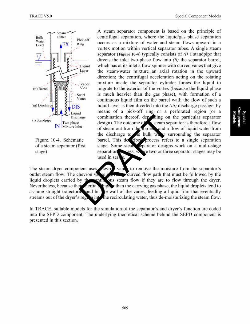
TRACE V5.0 Special Component Models FOOBAR1234FOOBAR1234
Special C
omponent
Models
A steam separator component is based on the principle ofcentrifugal separation, where the liquid/gas phase separationoccurs as a mixture of water and steam flows upward in avortex motion within vertical separator tubes. A single steamseparator (Figure 10-4) typically consists of (i) a standpipe thatdirects the inlet two-phase flow into (ii) the separator barrel,which has at its inlet a flow spinner with curved vanes that givethe steam-water mixture an axial rotation in the upwarddirection; the centrifugal acceleration acting on the rotatingmixture inside the separator cylinder forces the liquid tomigrate to the exterior of the vortex (because the liquid phaseis much heavier than the gas phase), with formation of acontinuous liquid film on the barrel wall; the flow of such aliquid layer is then diverted into the (iii) discharge passage, bymeans of a pick-off ring or a perforated region (or acombination thereof, depending on the particular separatordesign). The outcome of the steam separator is therefore a flowof steam out from the top exit and a flow of liquid water fromthe discharge to the bulk water surrounding the separatorbarrel. This described process refers to a single separationstage. Some steam separator designs work on a multi-stageseparation process, where two or three separator stages may beused in series.
The steam dryer component uses chevron vanes to remove the moisture from the separator’soutlet steam flow. The chevron vanes provide a curved flow path that must be followed by theliquid droplets carried by the continuous steam flow if they are to flow through the dryer.Nevertheless, because their inertia is higher than the carrying gas phase, the liquid droplets tend toassume straight trajectories and hit the wall of the vanes, feeding a liquid film that eventuallystreams out of the dryer’s region into the recirculating water, thus de-moisturizing the steam flow.
In TRACE, suitable models for the simulation of the separator’s and dryer’s function are codedinto the SEPD component. The underlying theoretical scheme behind the SEPD component ispresented in this section.
Vapor
LiquidLayer
Pick-off
Figure. 10-4. Schematic of a steam separator (first stage)
IN
EX
DIS
SteamOutlet
LiquidDischarge
Two-phaseMixture Inlet
SwirlVanes
Core
(i) Standpipe
(ii) Barrel
(iii) Discharge
Ring
BulkWaterLevel
DRAFT
509
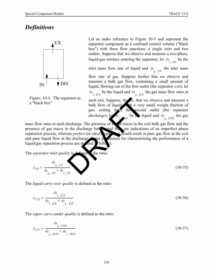
Special Component Models TRACE V5.0
Definitions
Let us make reference to Figure 10-5 and represent theseparator component as a confined control volume ("blackbox") with three flow junctions: a single inlet and twooutlets. Suppose that we observe and measure a two-phase,liquid-gas mixture entering the separator; let be the
inlet mass flow rate of liquid and the inlet mass
flow rate of gas. Suppose further that we observe andmeasure a bulk gas flow, containing a small amount ofliquid, flowing out of the first outlet (the separator exit); let
be the liquid and the gas mass flow rates at
such exit. Suppose, finally, that we observe and measure abulk flow of liquid, with a very small weight fraction ofgas, exiting from the second outlet (the separatordischarge); let be the liquid and the gas
mass flow rates at such discharge. The presence of liquid traces in the exit bulk gas flow and thepresence of gas traces in the discharge bulk liquid flow are indications of an imperfect phaseseparation process, whereas perfect (or ideal) separation would result in pure gas flow at the exitand pure liquid flow at the discharge. Some parameters for characterizing the performance of aliquid/gas separation process are defined as follows.
The separator inlet quality is defined as the ratio:
(10-35)
The liquid carry-over quality is defined as the ratio:
(10-36)
The vapor carry-under quality is defined as the ratio:
(10-37)
EX
IN DIS
Figure. 10-5. The separator as a "black box"
m·l IN,
m·g IN,
m·l EX,
m·g EX,
m·l DIS,
m·g DIS,
xIN
m·g IN,
m·g IN,
m·l IN,
+-------------------------------------=
xCO
m·l EX,
m·l EX,
m·g EX,
+----------------------------------------=
xCU
m·g DIS,
m·g DIS,
m·l DIS,
+-------------------------------------------=
DRAFT
510
TRACE V5.0 Special Component Models FOOBAR1234FOOBAR1234
Special C
omponent
Models
An ideal (perfect) separator would perform with xCO = 0 and xCU = 0. In reality, imperfectseparation always occurs and the performance characteristics of a separator component are oftenrepresented by expressing xCO and xCU as functions of xIN.
Conceptual Structure of the SEPD Component
In TRACE, the SEPD component is in effect a modified TEE for which a special solution isobtained at the joining cell (J-cell). The TRACE separator model can be ideally described asworking on two levels.
At the first conceptual level, the separator model is a "black-box" consisting of a control cell withthree flow junctions for the separator inlet (two-phase mixture), exit (wet steam) and discharge(bulk liquid with traces of gas) flows. At this "black-box" level, the TRACE separator/dryermodel triggers a special solution of the field equations to result, when possible, with theprescribed separator performance, given in terms of xCO and xCU, at exit and discharge junctions.
The separator performance parameters xCO and xCU are determined at the second conceptual levelof the model. At this specialized level, several options are available to the user for describing thephase separation process occurring "inside the black-box." These options range from the simplestapproach, that is the user-definition of constant xCO and xCU (including the particular case ofideal separation, where xCO = 0 and xCU = 0), to a more elaborated option consisting in the user-definition of variable xCO and xCU, to the mechanistic separator option, in which the separatorperformance is calculated by the code as a function of the local flow conditions, according to ananalytical model developed in past years by General Electric Co. Available at this second level isalso the dryers option, whose net result is a further modification of the SEPD xCO, based on acalculated dryer’s efficiency.
Assumptions
The TRACE separator model is based on the following assumptions, which are enforced in thecode:
1) Homogeneous flow at the exit and discharge flow junctions.
2) No phase change inside the SEPD component.
3) During regular SEPD operation, the void fraction of the jcell follows the void fraction of the cell J-1 (i.e., the void fraction history of the fluid in the separator barrel follows the void fraction history of the fluid in the standpipes).
4) Vertical configuration of the jcell.
Assumptions 1) and 2) are introduced during the derivation of the analytical model, as describedin the next section. During normal separator operation, the exit flow is expected to be in the mist
DRAFT
511

Special Component Models TRACE V5.0
regime (bulk gas carrying small liquid droplets) and the discharge flow is in the dispersed bubblesregime; for both situations, the assumption of homogeneous flow seems reasonable since the highinterfacial forces that are characteristic of finely dispersed flow regimes tend to equalize thephasic velocities. The assumption of no phase change is not expected to significantly deviate fromthe real flow behavior for two reasons; (1) because the separation process is rather quick and canbe approximated as adiabatic, and (2) because the incoming two-phase flow from the upperplenum mixing region can be assumed to be in thermal equilibrium.
Assumption 3) is introduced when the level tracking logic is applied to the SEPD component, asdescribed later. It allows for simulation of transient flow scenarios within the separator.Essentially, this assumption enforces the rule that the void fraction of the SEPD jcell (modelingthe separator barrel) follows closely the void fraction history of the incoming flow from cell J-1(standpipes), going to single-phase gas or liquid when the incoming flow also becomes singlephase. This assumption removes the possibility of non-physical results from the code when, forany reason, the incoming standpipe flow becomes single phase.
Assumption 4) is also introduced when the level tracking logic is applied to the SEPD componentand it is consistent with the usual configuration of steam separators in LWR plants.
Fundamental Analytical Model
At the "black-box" separator level, given the inlet flow conditions (phasic mass flow rates) andthe desired separator performance parameters (xCO and xCU), the goal is to determine the flowvariables at the exit and discharge junctions of the SEPD jcell.
Let us consider the relation between void fraction α and flow quality x at a given flow station(Ref. 10-7):
, (10-38)
where the slip ratio, S, is defined as the ratio between gas velocity over liquid velocity; ρ is thedensity and is the mass flow rate of the gas or liquid phase, as indicated by the subscript g or l,respectively. Writing Eq. (10-38) for the exit and discharge flow sections of a separator, assuminghomogeneous flow (S=1), yields:
(10-39)
and
α 1
1 1 x–x
----------- SρVρL------· ·+
----------------------------------------- x
x 1 x–( ) SρVρL------· ·+
---------------------------------------------m· V
m· V m· L SρVρL------· ·+
------------------------------------------= = =
m·
αEX
m·g EX,
m·g EX,
m·l EX,
ρVρL------·+
---------------------------------------------------=
DRAFT
512

TRACE V5.0 Special Component Models FOOBAR1234FOOBAR1234
Special C
omponent
Models
(10-40)
In Eq. (10-39) and (10-40), the phasic mass flow rates are the unknown variables that theseparator model must resolve. For this purpose, let us assume that no phase change occurs withinthe separator component and steady-state operation, so that the phasic mass flow rates areconserved within the separator:
(10-41)
(10-42)
By the definitions Eq. and of carry-over and carry-under qualities:
(10-43)
(10-44)
Equations (10-41), (10-42), (10-43) and (10-44) form a system of four algebraic, linear equationswith the four unknowns , , and . If the four equations are
independent, then a solution to the system exists and is unique. A way to obtain the solution toEq. (10-41) through (10-44) is the following:
Using Equations (10-43) and (10-44), let us define the total exit and discharge mass flowrates and , for which:
(10-45)
(10-46)
Similarly, it can be found that:
(10-47)
(10-48)
αDIS
m·g DIS,
m·g DIS,
m·l DIS,
ρVρL------·+
--------------------------------------------------------=
m·l IN,
m·l EX,
m·l DIS,
+=
m·g IN,
m·g EX,
m·g DIS,
+=
m·l EX,
m·l EX,
m·g EX,
+( ) xCO·=
m·g DIS,
m·l DIS,
m·g DIS,
+( ) xCU·=
m·l EX,
m·g EX,
m·l DIS,
m·g DIS,
m· EX m· DIS
m·l EX,
m· EX xCO·=
m·g DIS,
m· DIS xCU·=
m·g EX,
m· EX m·l EX,
– m· EX 1 x– CO( )·= =
m·l DIS,
m· DIS m·g DIS,
– m· DIS 1 x– CU( )·= =
DRAFT
513
Special Component Models TRACE V5.0
Entering the results of Equations (10-45), (10-46), (10-47) and (10-48) into (10-41) and (10-42),yields:
(10-49)
(10-50)
Equations (10-49) and (10-50) form a system of two linear algebraic equations, equivalent toEquations (10-41) through (10-44), in the unknowns and . It can be written in a morecompact matrix form:
(10-51)
If det(a) is non-zero, then the original Equations (10-41), (10-42), (10-43) and (10-44) areindependent and the unique solution of the system can be found by solving Eq. (10-51)(10-51).The algebraic system represented in Eq. (10-51) can be obtained, one among many ways, byemploying the following "shortcut" to invert a 2x2 square matrix (Ref. 10-11), in the followingway.
Let us define the matrix , obtained from A by inverting and switching the sign of the maindiagonal terms:
(10-52)
The solution to Equation (10-51) is given by:
(10-53)
where the reverse determinant is defined as:
m·l IN,
XCO m· EX· 1 XCU–( ) m· DIS·+=
m·g IN,
1 X– CO( ) m· EX· XCU m· DIS·+=
m· EX m· DIS
XCO 1 XCU–( )
1 X– CO( ) XCU
m· EX
m· DIS
m·l IN,
m·g IN,
=
A x b=
A
AX– CU 1 XCU–( )
1 X– CO( ) X– CO
=
m· EX
m· DIS
1rdet A( )--------------------- X– CU 1 XCU–( )
1 X– CO( ) X– CO
m·l IN,
m·g IN,
=
rdet A( ) 1 X– CO( ) 1 XCU–( ) XCU XCO·–·=
DRAFT
514

TRACE V5.0 Special Component Models FOOBAR1234FOOBAR1234
Special C
omponent
Models
Explicitly, the solution to Equation (10-53) is written as:
(10-54)
and
(10-55)
Finally, the individual phasic mass flow rates at the exit and discharge sections can be obtained byentering the solution to Equations (10-54) and (10-55) into the definitions from Equations(10-45), (10-46), (10-47) and (10-48). With that information available, and knowing the phasicdensities, the void fractions at the exit and discharge sections are also known by using Equations(10-39) and (10-40).
The knowledge of the void fractions αEX and αDIS is a key point in the TRACE separator model.In fact, once the values of the junction void fractions and phasic flow rates are determined fromthe prescribed xCO and xCU and inlet flow rates, then the TRACE separator model transfers theinformation into a modified solution scheme for the SEPD component. This modified solutionscheme relies on the computational framework that is available in TRACE for water leveltracking [See Chapter 6 Section Level Tracking of this manual].
In a nutshell, the TRACE level tracking logic can bedescribed by making reference to the schematic shownFigure 10-6.
For a computational cell where the presence of a waterlevel is detected, additional variables are introduced,among which are the void fractions αA and αB of theregions above and below the liquid/gas interface (andconvected through the two open edges of the cell). Then,within the level tracking framework, the field equationsare modified in order to make opportune use of thosevariables for the evaluation of the convected macroscopicquantities and the flux terms. From this description, itshould become clear how the separator model makes useof the Level Tracking framework. Figure 10-6 shows thelevel tracking structure that is applied on top of theseparator black-box. If the SEPD jcell (i.e., primary cell index where the secondary side connectsto the primary side) is viewed as a computational cell with a water level, and if the interface islocated above the discharge edge and below the exit edge, then the correspondence between thelevel tracking variables αA and αB and the separator model variables xCO and xCU can beintuitively recognized and is analytically identified by Equations (10-39) and (10-40), which havebeen previously derived formally.
m· EX1
rdet A( )--------------------- 1 XCU–( ) m·
g IN,XCU m·
l IN,·–·=
m· DIS1
rdet A( )--------------------- 1 XCO–( ) m·
l IN,XCO m·
g IN,·–·=
J
EX
IN DIS
αA=αEX
αB=αDISαJ
Figure. 10-6. Level Tracking Framework applied on top of the Separator "black box"
DRAFT
515
Special Component Models TRACE V5.0
The application of the level tracking logic to the SEPD jcell presents two complications in that (i)the jcell has three flow junctions to the neighboring cells, whereas a regular 1D level tracking cellhas only two junctions, and that (ii) no information is given about the average void fraction of theSEPD jcell and its value would remain undetermined for this black-box type of separator.
The first difference is overcome when the discharge velocity at the jcell side junction, which isassumed common to both phases, is imposed to the solution rather than addressed by the leveltracking logic. The magnitude of the homogeneous discharge velocity is obtained from theconsiderations discussed earlier (assuming balanced inlet and outlet flow rates) and depends onthe prescribed separator performance:
(10-56)
where FA is the flow area of the discharge section and the phasic mass flow rates are given byEquations (10-46), (10-48) and (10-55) as functions of the separator performance parameters andinlet flow rates.
To address the second complication regarding the determination of the jcell average void fraction,the magnitude of the discharge velocity is adjusted within the separator model logic (with asimple proportional control scheme) in order to impose an additional restrictive condition that thedifference between the void fraction in the jcell and the void fraction in the adjacent cell from theinlet side (cell j-1) be minimized. That is, the discharge velocity is used to regulate the voidfraction of the jcell, in such way that the jcell void fraction follows as close as possible a targetvalue, which is chosen to be the void fraction of the cell preceding the jcell (in the direction of thetwo-phase flow entering the SEPD jcell in regular operation).
Two facts should be noted in conclusion. First, the assumption of balanced inlet and outlet massflows is used to calculate the void fractions and an initial value for the discharge velocity; thatassumption is then "dropped" when the discharge velocity is changed and adjusted to control thejcell void fraction. Thus, the TRACE separator model effectively allows for non-equilibrium inletand outlet flows, with transient mass accumulation or removal from the SEPD jcell. In fact, logicis implemented in the code to bypass the separator model (and the SEPD component becomes aregular TEE) during a calculation when the local flow conditions become inconsistent with theregular function of flow separation, such as for situations of single phase flow or reversed flows(when the jcell void fraction becomes 1 or 0 or the velocities change sign). This feature of themodel is explained in detail in the TRACE User’s Guide. Finally, it should be noted that the leveltracking framework is applied "on top of the black box," in order to reproduce and enforce in thecode a phase separation process, given some performance parameters as input. Therefore, theapplication of the level tracking is not an attempt to model the underlying physics of the two-phase flow separation occurring "inside the black box." This latter task of describing the separatorperformance is left to the user, with the option of using a more mechanistic model.
VH DIS,
m·V DIS,
αDIS FA ρV·( )·-----------------------------------------
m·L DIS,
1 αDIS–( ) FA ρL··--------------------------------------------------= =
DRAFT
516
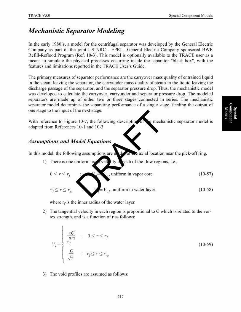
TRACE V5.0 Special Component Models FOOBAR1234FOOBAR1234
Special C
omponent
Models
Mechanistic Separator Modeling
In the early 1980’s, a model for the centrifugal separator was developed by the General ElectricCompany as part of the joint US NRC - EPRI - General Electric Company sponsored BWRRefill-Reflood Program (Ref. 10-3). This model is optionally available to the TRACE user as ameans to simulate the physical processes occurring inside the separator "black box", with thefeatures and limitations reported in the TRACE User’s Guide.
The primary measures of separator performance are the carryover mass quality of entrained liquidin the steam leaving the separator, the carryunder mass quality of steam in the liquid leaving thedischarge passage of the separator, and the separator pressure drop. Thus, the mechanistic modelwas developed to calculate the carryover, carryunder and separator pressure drop. The modeledseparators are made up of either two or three stages connected in series. The mechanisticseparator model determines the separating performance of a single stage, feeding the output ofone stage to the input of the next stage.
With reference to Figure 10-7, the following description of the mechanistic separator model isadapted from References 10-1 and 10-3.
Assumptions and Model Equations
In this model, the following assumptions are made for the axial location near the pick-off ring.
1) There is one uniform axial velocity in each of the flow regions, i.e.,
: , uniform in vapor core (10-57)
: , uniform in water layer (10-58)
where rf is the inner radius of the water layer.
2) The tangential velocity in each region is proportional to C which is related to the vor-tex strength, and is a function of r as follows:
(10-59)
3) The void profiles are assumed as follows:
0 r rf≤ ≤ Va Vag=
rf r rw≤ ≤ Va Vaf=
Vt
rC
rf3 2⁄
---------- ; 0 r rf≤ ≤
Cr
------ ; rf r rw≤ ≤⎩⎪⎪⎪⎨⎪⎪⎪⎧
=
DRAFT
517

Special Component Models TRACE V5.0
(10-60)
and
Figure. 10-7. Schematic of first stage of mechanistic separator.
HD
Hsk
H12
Standpipe
HUB Van
rw
Vaporcore
VD
Liquid layer
rr
rfVaf
Vag
Pickoff ring
Discharge passage
Vi,Pi,ρmi
α1 b r
rw-----– ; 0 r rf≤ ≤
arwr
----- 1–⎝ ⎠⎛ ⎞ ; rf r rw≤ ≤
⎩⎪⎪⎨⎪⎪⎧
=
DRAFT
518
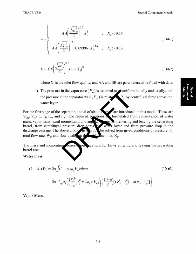
TRACE V5.0 Special Component Models FOOBAR1234FOOBAR1234
Special C
omponent
Models
(10-61)
(10-62)
where Xi is the inlet flow quality, and AA and BB are parameters to be fitted with data.
4) The pressure in the vapor core ( ) is assumed to be uniform radially and axially, and
the pressure at the separator wall ( ) is related to by centrifugal force across the water layer.
For the first stage of the separator, a total of six unknowns are introduced in this model. These areVag, Vaf, C, rf, Po, and Pw. The required equations are formulated from conservation of watermass, vapor mass, axial momentum, and angular momentum entering and leaving the separatingbarrel, from centrifugal pressure drop across the water layer and from pressure drop in thedischarge passage. The above unknowns can now be solved from given conditions of pressure, Pi,total flow rate, Wi, and flow quality at the swirl vane inlet, Xi.
The mass and momentum conservation equations for flows entering and leaving the separatingbarrel are:
Water mass.
(10-63)
Vapor Mass.
aAA
grw2
C-------------
⎝ ⎠⎜ ⎟⎛ ⎞
0.5
Xi2 ; Xi 0.15<
AAgrw
2
C-------------
⎝ ⎠⎜ ⎟⎛ ⎞
0.5
0.09335( )Xi0.75 ; Xi 0.15>
⎩⎪⎪⎪⎨⎪⎪⎪⎧
=
b BBgrw
2
C-------------
⎝ ⎠⎜ ⎟⎛ ⎞
0.5
1 Xi–( )3=
Po
Pw Po
1 Xi–( )Wi 2π 1 α–( )ρfVar rd∫
2πVagρf13---rfbrw-------⎝ ⎠
⎛ ⎞ rf2 2ρf πVaf
1 a+2
------------⎝ ⎠⎛ ⎞ rw
2 rf2–( ) a rw rf–( )–[ ]
⎩ ⎭⎨ ⎬⎧ ⎫
+
= =
DRAFT
519

Special Component Models TRACE V5.0
(10-64)
Angular Momentum.
(10-65)
Axial Momentum.
(10-66)
Assuming that the flow through the swirl vane passages is homogeneous and that the swirl vanepassages act as a nozzle, the pressure and velocity entering the separating barrel are related to theconditions in the standpipe as follows.
(10-67)
(10-68)
(10-69)
where θ is the angle between the swirl vanes and the horizontal plane, ρmi is the inlet mixturedensity, and CNOZ is the contraction loss coefficient defined as:
(10-70)
where An is the swirl vane flow area and Ai is the standpipe flow area.
XiWi 2π αρgVgr rd0
rw
∫
2πρgVag12--- 1
3---b
rfrw-----–⎝ ⎠
⎛ ⎞ rf2 2πρgVaf a
12--- rw rf–( )2 .+
= =
Vtnr 2πrρmiVan( ) rdrh
rw
∫ Vtr 2πrρVa( ) r Ftrw+d0
rw
∫=
πrh2Po 2π ρmiVan
2 Pn+( )r rd0
rw
∫ 2π ρVa2 P+( )r r Fa+d
0
rw
∫= =
Wi ρmiVi Ai ρmiVan An= =
Pi12---ρmiVi
2+ Pn12---ρmi Van
2 Vtn2+( ) 1 CNOZ+( )+=
VanVtn--------- θtan=
CNOZ 0.5 1AnAi-------–⎝ ⎠
⎛ ⎞=
DRAFT
520

TRACE V5.0 Special Component Models FOOBAR1234FOOBAR1234
Special C
omponent
Models
Fa and Ft in Eq. (10-65) and Eq. (10-66) are the axial and tangential components of the frictionalforce on the swirling water layer,
(10-71)
(10-72)
where Vtw is the tangential velocity on the wall,
(10-73)
and Vw is the resultant swirling velocity on the wall,
(10-74)
Ff is the resultant frictional force,
(10-75)
Assuming that the liquid film is thin with respect to the radius of curvature of the separator barrel,the flow can be considered to be film flow over a flat plate. For turbulent flow over a flat plate,
(10-76)
where ReL is defined as
(10-77)
The radial pressure drop across the water layer due to centrifugal force is
(10-78)
Fa Ff
VafVw--------
⎝ ⎠⎜ ⎟⎛ ⎞
=
Ft Ff
VtwVw---------
⎝ ⎠⎜ ⎟⎛ ⎞
=
VtwCrw
---------=
Vw Vtw2 Vaf
2+=
Ff12---ρfCFVw
2 2πrw( )HD=
CF0.455
ReLlog( )2.58-------------------------------=
ReLρVwµ
-----------HDVwVaf
----------------=
PdP0
Pw
∫ ρVt
2
r------ rd
rf
rw
∫=
DRAFT
521

Special Component Models TRACE V5.0
or
(10-79)
The pressure drop in the discharge passage is
(10-80)
where ρM,D and VD are the mixture density and velocity in the discharge passage, HD and DD arethe length of the separator barrel and hydraulic diameter of the discharge passage, EFFLD is theeffective L/D coefficient at the pick-off ring, CK is the total loss coefficient in the dischargepassage, H12 is the height of the liquid pool surrounding the separator relative to the bottom of thedischarge passage, and Hsk is the axial distance between the separator hub and the bottom of thedischarge passage.
For the discharge passage,
(10-81)
The steam and water flows discharged through the discharge passage are calculated as follows:
(10-82)
(10-83)
For a water layer thicker than the gap between the pick-off ring and the separator barrel, i.e.,rf < rr, the steam and water flows through the discharge passage are
Po Pw ρf a ρf ρg–( )+[ ]C2 1rf---- 1
rw-----–⎝ ⎠
⎛ ⎞– a ρf ρg–( )C2 rwrf----- 1
rr---- 1
rw-----–⎝ ⎠
⎛ ⎞+=
12---ρVa
2 P+⎝ ⎠⎛ ⎞
rr
rw
∫ dA
Adrr
rw
∫------------------------------------------ 1
2---ρ
M D,VD
2 1 2CFHDDD-------- EFFLD+⎝ ⎠
⎛ ⎞ CK+ +
Po ρfgH12 ρD– g HD Hsk+( )+[ ]
+=
CF0.079
Re0.25---------------=
Wg cu,
2π αρgVar rdrr
rw
∫=
Wf cu,
1 α–( )ρfVar rdrr
rw
∫=
DRAFT
522

TRACE V5.0 Special Component Models FOOBAR1234FOOBAR1234
Special C
omponent
Models
(10-84)
(10-85)
For a water layer thinner than the gap between the pick-off ring and the separator barrel wall, i.e.,rr < rf, the liquid and vapor flow rates in the discharge passage are
(10-86)
(10-87)
The steam and water flows leaving the present stage and entering the next stage are
(10-88)
(10-89)
The total discharge flow is
(10-90)
Assuming homogeneous flow in the discharge passage, the mean void fraction is
, (10-91)
the mixture density in the discharge passage is
ρM,D = αcuρg + (1 - αcu)ρf (10-92)
and the velocity in the discharge passage is
. (10-93)
Wg cu,
πρgVafa rw rw–( )2=
Wf cu,
πρfVaf rw2 rr
2–( ) a rw rr–( )2–[ ]=
Wg cu,
XiWi 2πρgVag12--- 1
3---b
rrrw-----–⎝ ⎠
⎛ ⎞–= rr2
Wf cu,
1 Xi–( )Wi 2πρfVagrr2 1
2---⎝ ⎠
⎛ ⎞ brrrw-----–=
Wg co,
steam flow( )in Wg cu,
–=
Wf co,
water flow( )in Wf cu,
–=
WD Wg cu,
Wf cu,
+=
αcu
Wg cu,
Wg cu,
Wf cu,
ρgρf-----+
--------------------------------------------=
VDWD
ρM D,
AD----------------------=
DRAFT
523

Special Component Models TRACE V5.0
In summary, for given swirl vane inlet conditions, Pi, Xi, and Wi, the unknowns Vag, Vaf, C, rf,Po, and Pw are calculated by solving Equations Eq. (10-63) to Eq. (10-80) simultaneously.
Similar equations can be written for the second- and third-stages. Since it is assumed that Po isuniform axially, i.e., the vapor core pressure drop in the axial direction is small, the axialmomentum equation can be neglected in the solution for the upper stages. For these stages, theunknowns are reduced to Vag, Vaf, C, rf, and Pw, and the equations are the conservation of watermass, vapor mass, angular momentum, the pressure drop across the water layer, and the pressuredrop in the discharge passage.
The right hand sides of Equations Eq. (10-63), Eq. (10-64), and Eq. (10-65) represent the waterflow, vapor flow, and angular momentum entering the separator barrel. For the second- and third-stages, these terms are modified as follows:
(10-94)
Carryover and Carryunder Qualities
The total vapor flow that is carried under consists of two parts; i.e., the steam flow through thefirst discharge passage which discharges its fluid below the liquid level and the steam entrainedby the water discharged from higher stages. The exits of the discharge passages of the higherstages are located above the liquid level. It is assumed that the entrainment is proportional to thesquare of the total water flow discharged from the higher stages, i.e.,
(10-95)
where N=2 for a two-stage separator, N=3 for a three-stage separator and CC is a constant to befitted with data.
The total water that is carried over consists of two parts, the water flow through the last stage andthe water flow entrained by the steam discharged from the higher stages through their dischargepassages. Similarly, the second part is assumed to be proportional to the square of the total steamflow discharged from the higher stages, i.e.,
Water flow( )in Wf co,
( )previous stage
=
Steam flow( )in Wg co,
( )previous stage
=
Angular momentum( )in Vtr 2πρVa( )r rd0
rr
∫previous stage
.=
Wg cu,⎝ ⎠
⎛ ⎞total
Wg cu,⎝ ⎠
⎛ ⎞1
CC Wf cu,⎝ ⎠
⎛ ⎞i
2
i 2=
N
∑+=
DRAFT
524

TRACE V5.0 Special Component Models FOOBAR1234FOOBAR1234
Special C
omponent
Models
(10-96)
where DD is a constant to be fitted with data.
The carryunder and carryover are defined as
(10-97)
The parameters AA, BB, CC, and DD were tuned to fit the available test data (Refs. 10-4, 10-5,and 10-6) for two- and three-stage separators. Table 10-2 summarizes the values for theseparameters.
Dryer Modeling
This description is taken from Reference 10-1.
The steam dryer uses chevron vanes to remove the moisture which is discharged from the steamseparators. The vanes provide a curved path which the liquid droplets must follow if they are toflow through the dryer. If the interfacial force is too low, it cannot drag the liquid droplets alongthe curved path due to their inertial and they hit the vanes, are de-entrained, and the resultantliquid film flows down the vanes under the force of gravity into collecting trays and then back tothe liquid pool surrounding the separators. If the vapor velocity is high, it exerts a larger
Table 10-2. Summary of fitted parameters in the mechanistic separator model.
2-Stage Separator 3-Stage Separator
Parameter 1st Stage 2nd Stage 1st Stage 2nd Stage 3rd Stage
AA 110. 20. 110. 20. 20.
BB 0.5 0.25 0.5 0.25 0.55
CC 0.0004 --- 0.0004 --- ---
DD 0.009 --- 0.11 --- ---
Wf co,⎝ ⎠
⎛ ⎞total
Wf co,⎝ ⎠
⎛ ⎞N
DD Wg cu,⎝ ⎠
⎛ ⎞i
2
i 2=
N
∑+=
CU
Wg cu,⎝ ⎠
⎛ ⎞total
Total downward water flow------------------------------------------------------------------------=
CO
Wf co,⎝ ⎠
⎛ ⎞total
Total upward steam flow------------------------------------------------------------------ .=
DRAFT
525

Special Component Models TRACE V5.0
interfacial force on the droplets and more of the entrained liquid gets through the dryer vanes.Thus the dryer efficiency depends on the steam velocity and the moisture content of the steamflow entering the dryer. For a given steam inlet velocity, there is a critical dryer inlet moisture.Good moisture separation is achieved if the inlet moisture is lower than the critical value. If theinlet moisture is above the critical value, the dryer separating capacity is exceeded and themoisture can pass through the dryer.
The dryer capacity is simulated by a capacity factor GDRY which is defined in the following way.For a given steam velocity V at the inlet to the dryer, the critical dryer inlet moisture CDIM iscalculated as:
(10-98)
where CDIM is the critical inlet moisture, VDRY1 is the vapor velocity below which any amountof moisture is assumed to be separated from the vapor stream, and VDRY2 is the vapor velocityabove which no amount of moisture, however small, can be separated from the vapor stream.
The dryer inlet moisture (DIM) is computed assuming homogeneous flow as
(10-99)
where αg, ρf, and ρg are the vapor void fraction, liquid density, and the vapor density in the dryer.
The capacity factor GDRY is defined as
(10-100)
where DELDIM is the range of inlet moisture over which the dryer capacity goes from one to zerofor a fixed vapor inlet velocity. These relations are shown schematically in Figure 10-8.
CDIM
1 ; V VDRY1≤
1 V VDRY1–VDRY2 VDRY1–--------------------------------------------------– ; VDRY1 V VDRY2< <
0 ; V VDRY2≥⎩⎪⎪⎪⎨⎪⎪⎪⎧
=
DIM 1αg
αg 1 αg–( )ρfρg-----+
--------------------------------------–=
GDRY
1 ; DIM CDIM≤
1 CDIM DIM–DELDIM
------------------------------------+ ; CDIM DIM CDIM DELDIM+( )<<
0 ; DIM CDIM DELDIM+( )≥⎩⎪⎪⎪⎨⎪⎪⎪⎧
=
DRAFT
526
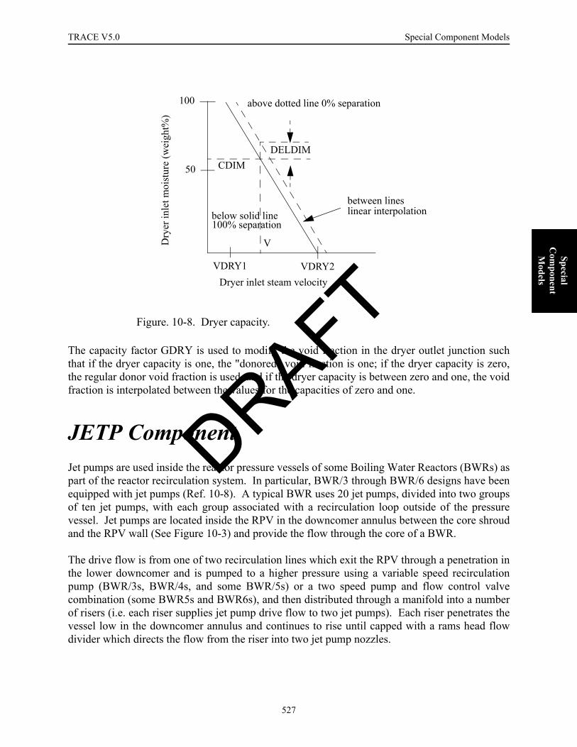
TRACE V5.0 Special Component Models FOOBAR1234FOOBAR1234
Special C
omponent
Models
The capacity factor GDRY is used to modify the void fraction in the dryer outlet junction suchthat if the dryer capacity is one, the "donored" void fraction is one; if the dryer capacity is zero,the regular donor void fraction is used, and if the dryer capacity is between zero and one, the voidfraction is interpolated between the values for the capacities of zero and one.
JETP ComponentJet pumps are used inside the reactor pressure vessels of some Boiling Water Reactors (BWRs) aspart of the reactor recirculation system. In particular, BWR/3 through BWR/6 designs have beenequipped with jet pumps (Ref. 10-8). A typical BWR uses 20 jet pumps, divided into two groupsof ten jet pumps, with each group associated with a recirculation loop outside of the pressurevessel. Jet pumps are located inside the RPV in the downcomer annulus between the core shroudand the RPV wall (See Figure 10-3) and provide the flow through the core of a BWR.
The drive flow is from one of two recirculation lines which exit the RPV through a penetration inthe lower downcomer and is pumped to a higher pressure using a variable speed recirculationpump (BWR/3s, BWR/4s, and some BWR/5s) or a two speed pump and flow control valvecombination (some BWR5s and BWR6s), and then distributed through a manifold into a numberof risers (i.e. each riser supplies jet pump drive flow to two jet pumps). Each riser penetrates thevessel low in the downcomer annulus and continues to rise until capped with a rams head flowdivider which directs the flow from the riser into two jet pump nozzles.
Figure. 10-8. Dryer capacity.
100
50D
ryer
inle
t moi
stur
e (w
eigh
t%)
above dotted line 0% separation
below solid line100% separation
Dryer inlet steam velocity
DELDIMCDIM
VDRY1 VDRY2
V
between lineslinear interpolation
DRAFT
527

Special Component Models TRACE V5.0
The high velocity and relatively high momentum flow through the drive line nozzle entrains fluidfrom the downcomer into the suction of the jet pump. The two flows (i.e. drive and suction)merge together in the jet pump throat or mixing section. The diffuser section below the mixingsection recovers some of the velocity head as static head and discharges the merged flow into thelower plenum. The suction flow can be as large as twice the magnitude of the drive flow. Themajor components within a jet pump are given in Figure 10-9.
The JETP component is a special case of a TEE component. The TRACE JETP componentassumes that the users have defined the geometric input for the major components for a jet pump(i.e. drive line, drive nozzle, throat or mixing section, diffuser, and tail pipe). Based on the userspecified geometry, the JETP component calculates irreversible loss factors for the smooth areachanges associated with the nozzle and diffuser. The user input for flow loss factors is replacedwith flow loss factors based on Idel’Chik (Ref. 10-9) for smooth area expansions and contractionsfor all of the cell edges internal to the JETP component (i.e. not component boundary cell edges).Component boundary cell edges are at the suction inlet, the discharge outlet, and the inlet to driveline. Only the user input for these three component boundary cell edges will not be overwrittenby the JETP component internal irreversible loss factor logic.
For an expansion through a smooth area change, the irreversible loss factor based on Idel’Chik is:
(10-101)
where,
Ke = Expansion irreversible loss factor.Ce = Expansion constant.α = Angle of the diffuser.A* = Area ratio of outlet to inlet flow area.
For contraction through a diffuser/nozzle the irreversible loss factor is:
(10-102)
where,
Kc = Contraction irreversible loss factor.Cc = Contraction constant.
Based on comparison with the data given in Reference 10-10, expansion and contractionconstants were found to be Ce = 5.5 and Cc = 0.38, respectively. The angle of the diffuser is givenby the following formula:
(10-103)
Ke Ce αtan( )1.5 1 A∗–( )2=
Kc Cc α 1 A∗–( )sin=
α HD j 1+( ) HD j( )–2DX j( )
------------------------------------------------atan=
DRAFT
528
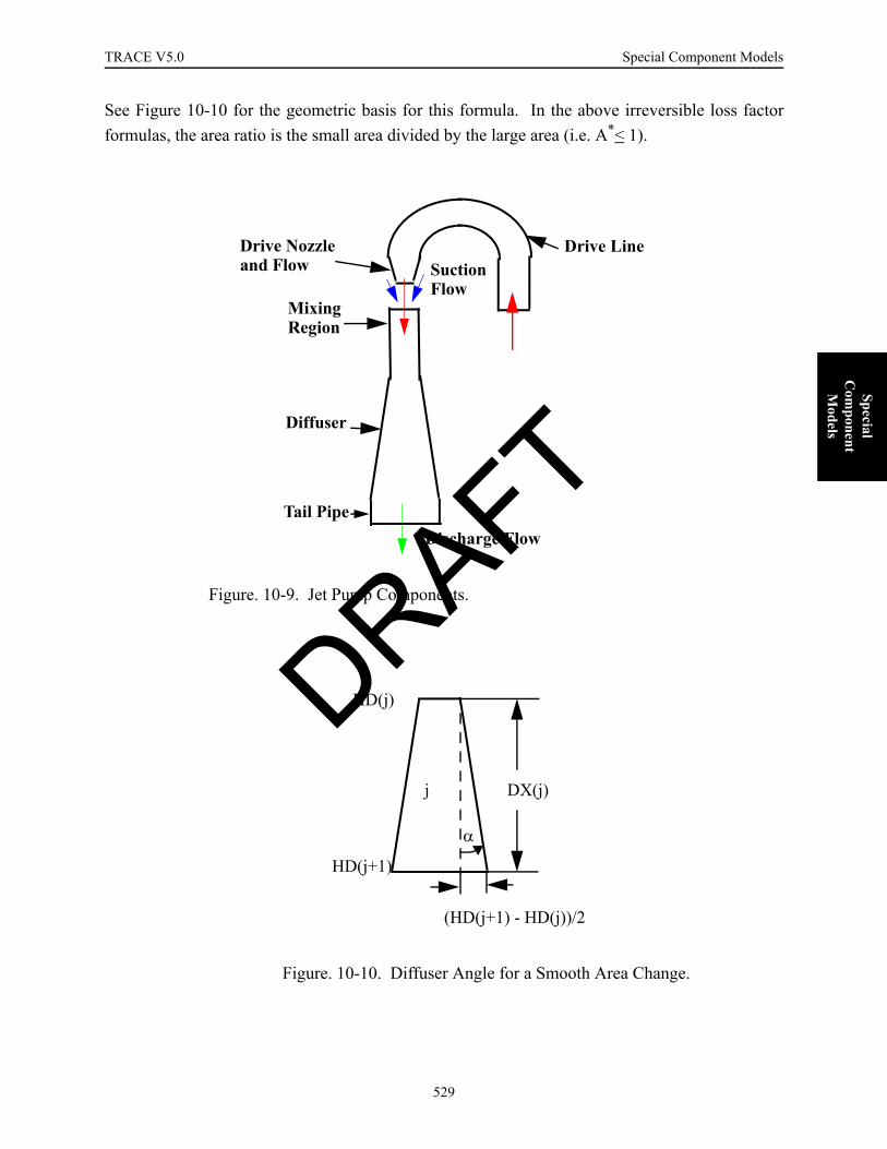
TRACE V5.0 Special Component Models FOOBAR1234FOOBAR1234
Special C
omponent
Models
See Figure 10-10 for the geometric basis for this formula. In the above irreversible loss factorformulas, the area ratio is the small area divided by the large area (i.e. A*< 1).
Figure. 10-9. Jet Pump Components.
Figure. 10-10. Diffuser Angle for a Smooth Area Change.
Tail Pipe
Diffuser
MixingRegion
Drive LineSuctionFlow
Drive Nozzleand Flow
Discharge Flow
j DX(j)
(HD(j+1) - HD(j))/2
α
HD(j)
HD(j+1)
DRAFT
529
Special Component Models TRACE V5.0
The mixing and nozzle losses are due to the incomplete mixing of the high velocity drive nozzlewith the low velocity suction flow. The mixing and nozzle loss model for the JETP componentdepends upon the flow configuration or flow regime. There are six possible steady-state flowregimes for a jet pump, in terms of the direction of the flow at the nozzle, suction, and dischargeof the jet pump or normal and off-normal operation of a jet pump. Three flow configurations forpositive drive nozzle flow and three flow regime configurations for negative drive nozzle flow aregiven in Figure 10-11. The M ratio in Figure 10-11 is defined as:
(10-104)
where,
Wd = Liquid mass flow rate in the drive nozzle of the jet pump.Ws = Liquid mass flow rate in the suction of the jet pump.Wds = Liquid mass flow rate in the discharge of the jet pump.
The mixing loss and nozzle loss formulas for the flow dependent irreversible losses are given inTable 10-3 and are based on comparison to data (Ref. 10-10). For the jcell of the JETPcomponent, where the drive flow and suction mixes, there are three momentum cells (i.e. one foreach cell edge - drive nozzle, suction, and discharge). The jcell of a TEE component, is the cellwhere the secondary side connects to the primary side. The mixing loss factor given in Table10-3 is applied to the discharge cell edge for the jcell control volume given in Figure 10-12. The
Table 10-3. Mixing, Nozzle, and Suction Irreversible Losses
Regime
Mixing Losses
Nozzle Losses
Suction
1 0 0 0
2 0
3 0
4 0 0
5 0
6 0 2.55
∆P
ρ Vd( )2----------------- ∆P
ρ Vd( )2----------------- ∆P
ρ Vs( )2-----------------
0.3 M2·– M 0.08 M· 0.06–( )·[ ]
0.1 0.0333 M·–( )– Min 2.5 M, 0.08 M· 0.06–( )·[ ]
Max 0 0.48, M 0.33 0.055 M·–( )·–[ ]
0.48 M 0.33 1.74 M·–( )·–[ ] AsAds---------⎝ ⎠
⎛ ⎞2
1–⎝ ⎠⎛ ⎞
AsAds---------⎝ ⎠
⎛ ⎞2
1–⎝ ⎠⎛ ⎞
MWdWs--------= DRAFT
530
TRACE V5.0 Special Component Models FOOBAR1234FOOBAR1234
Special C
omponent
Models
Figure. 10-11. Jet Pump Flow Regimes or Configurations
DriveSuction
M > 0Wd > 0Ws > 0
Regime 1
DriveSuction
-1 < M < 0Wd > 0Ws < 0
Regime 2
DriveSuction
M < -1Wd > 0Ws < 0
Regime 3
Wds > 0 Wds > 0 Wds < 0
Positive Drive Nozzle Flow
DriveSuction
M > 0Wd < 0Ws < 0
Regime 4
DriveSuction
-1 < M < 0Wd < 0Ws > 0
Regime 5
DriveSuction
M < -1Wd < 0Ws > 0
Regime 6
Wds < 0 Wds < 0 Wds > 0
Discharge Discharge Discharge
Negative Drive Nozzle Flow
DRAFT
531
Special Component Models TRACE V5.0
nozzle loss factor given in Table 10-3 is applied to the drive nozzle cell edge for the jcell controlvolume given in Figure 10-12. The suction loss factor is applied to the suction cell edge given inFigure 10-12. The loss factors given in Table 10-3 may be positive or negative and have beendetermined based on experimental data to be the correction required for the 1D TRACEmomentum solution to be consistent with the multi-dimensional flow within a jet pump.
TRACE results for the INEL 1/6th scale jet pump for the M-N curve is given in Figure 10-13 andis consistent with experimental data for that test facility. The M-ratio in Figure 10-13 is given byEq. (10-104) and the N-Ratio in Figure 10-13 is given by Eq. (10-105). The N-ratio is the ratio ofthe specific energy increase of the suction flow divided by the specific energy decrease of thedrive nozzle flow.
(10-105)
where,
Pds is the pressure in the discharge of the jet pump.Pd is the pressure in the drive line of the jet pump.Ps is the pressure in the suction of the jet pump.Vd is the velocity in the drive nozzle.ρ is the density in the drive nozzle.
In Figure 10-13 there is one curve for positive flow in the drive nozzle and one curve for negativeflow in the drive nozzle. The six flow regimes identified in Figure 10-11 are covered by the twocurves in Figure 10-13, except for Regime 3 (i.e. positive drive flow with M < -1). There is adiscontinuity in the mixing loss between regimes 2 and 3 at M = -1, which will be addressed in afuture version of the TRACE computer code.
Figure. 10-12. JCELL or Mixing Cell Control Volume
NPds Ps–
Pd Pds–ρVd
2
2------------+
----------------------------------------=
DischargeDrive Nozzle
Suctionjcell
Ad
AsAds
DRAFT
532

TRACE V5.0 Special Component Models FOOBAR1234FOOBAR1234
Special C
omponent
Models
References10-1 K. E. Carlson, R. A. Riemke, S. Z. Rouhani, R. W. Shumway, and W. L. Weaver,
“RELAP5/MOD3 Code Manual — Volume 1: Code Structure, System Models, andSolution Methods,” Idaho National Engineering Laboratory report NUREG/CR-5535,EGG-2596 (Draft), June 1990.
10-2 V. L. Streeter and E. B. Wylie, Hydraulic Transients, (McGraw-Hill Book Company, NewYork, New York, 1967) pp. 151–160.
10-3 Y. K. Cheung, V. Parameswaran, and J. C. Shaug, "BWR Refill-Reflood Program, Task4.7-Model Development, TRAC-BWR Component Models," NUREG/CR-2574, EPRINP-2376, GEAP-22052, April 1983.
10-4 R. H. Moen, et al., “Advances in Boiling Water Reactor Steam Separator Systems,”ASME-60-WA/NE-5, November 1969.
10-5 E. L. Burley, “Performance of Internal Steam Separator System in Boiling WaterReactors,” ASME-69-WA/NE-24, November 1969.
10-6 S. Wolf and R. H. Moen, “Advances in Steam-Water Separators for Boiling WaterReactors,” ASME-73-WA/PWR-4, November 1973.
Figure. 10-13. M-N Curve for INEL 1/6th Scale Jet Pump
-3
-2
-1
0
1
2
3
-2 -1 0 1 2 3
M Ratio
N r
ati
oPositive
Negative
DRAFT
533

Special Component Models TRACE V5.0
10-7 N. Todreas and M. S. Kazimi, "Nuclear Systems I - Thermal Hydraulic Fundamentals",Taylor&Francis Publ., second printing 1993.
10-8 R.T. Lahey, Jr, and F. J. Moody, "The Thermal-Hydraulics of a Boiling Water Reactor,"ANS, 1977.
10-9 Idel’Chik, "Handbook of Hydraulic Resistance Coefficient of Local Resistance andFriction," AEC-TR-6630(1966).
10-10 Wilson, G.E., "INEL One-Sixth Scale Jet Pump Data Analysis," EGG-CAAD-5357(February 1981).
10-11 Weisstein, Eric W. "Matrix Inverse." From MathWorld — A Wolfram Web Resource, http://mathworld.wolfram.com/MatrixInverse.html
DRAFT
534
TRACE V5.0 Fluid Properties FOOBAR1234FOOBAR1234FOOBAR1234
Fluid Properties
11 Fluid Properties
FOOBAR1234FOOBAR1234FOOBAR1234FOOBAR1234
TRACE can model several different working fluids as well as multiple non-condensable gasspecies. The fluids available in TRACE are H20 (Refs. 11-1, 11-5, and 11-9), D20, Na, PbBi, andthe following noncondensable gases, or predefined mixtures of these gases: air, argon, helium,hydrogen, krypton, nitrogen, xenon, and non-ideal helium. With regards to the properties forwater, TRACE offers two schemes by which those properties can be obtained — either frompolynomial fits to steam-table data (the default method), or from interpolation of the steam tabledata that conforms to the IAPWS-95 standard. Water properties presented in later sections of thischapter refer to the original TRACE water properties which are based on polynomial fits tosteam-table data for water. Information about the IAPWS-95 water properties can be found in theoriginal source (Ref. 11-9). Tables 11-1 through 11-11, which list the values of the constants usedto obtain property values, are provided throughout this chapter.
Nomenclature = constant-pressure specific heat (J · kg–1 · K–1)
= constant-volume specific heat (J · kg–1 · K–1)
= internal energy
= change in energy required to move along the isotherm at between two
different pressure values
= enthalpy
= latent heat of vaporization
= enthalpy of evaporation
= thermal conductivity
= numerical constant
= pressure (Pa)
= saturation pressure corresponding to Tl
cp
cv
e
ELP T1
h
hlv
hlvs
k
M
p
PSL
DRAFT
535

Fluid Properties TRACE V5.0
= gas constant (J · kg–1 · K–1)
= temperature (K)
= specific volume
= ratio of specific heats
= viscosity
= density
= surface tension
Subscripts = noncondensable gas
= approximate
= critical
= gas
= ideal gas behavior
= liquid
= steam-gas mixture
, = saturation
= steam
Thermodynamic PropertiesThe input variables to the TRACE equation-of-state (EOS) package are the total pressure; thepartial pressure of the noncondensable gas, if any is present; and the liquid- and gas-phasetemperatures, where the gas phase is either steam, a noncondensable gas, or a steam-gas mixture.The output variables include the saturation temperature corresponding to the total pressure and itsderivative with respect to the total pressure; the saturation temperature corresponding to thepartial pressure of steam and its derivative with respect to the steam partial pressure; the internalenergies and densities of the liquid and gas phases, and their partial derivatives with respect topressure (at constant temperature) and with respect to temperature (at constant pressure); and,finally, the saturated liquid and saturated steam enthalpies and their derivatives with respect topressure.
The TRACE EOS package supplies thermodynamic properties valid for temperatures andpressures within the following ranges:
(11-1)
R
T
v
γ
µ
ρ
σ
a
approx
critical
g
ideal
l
m
sat s
v
273.15 K Tl 713.94025779311 K ,≤ ≤
DRAFT
536

TRACE V5.0 Fluid Properties FOOBAR1234FOOBAR1234FOOBAR1234
Fluid Properties
(11-2)
and
(11-3)
If the EOS package is provided with data outside this range, it adjusts the data to thecorresponding limit and issues a warning message.
Equations for the various properties used in TRACE are given below. Tables 11-1 through 11-6list the values of the constants.
Saturation Properties
Relationship Between Saturation Temperature and Pressure
Four temperature and pressure regions are used to evaluate the saturation pressure, saturationtemperature, and derivative of saturation temperature with respect to saturation pressure.
610.8 Pa ≤ ps< 90.56466 × 10³ Pa and 273.15 K ≤ Ts < 370.4251 K
A linear function of temperature accurately represents the enthalpy of evaporation such that
(11-4)
for all (corresponding to all ). The Clausius-Clapeyronequation, which assumes that steam is an ideal gas and neglects liquid volume compared to steamvolume, can be written as
(11-5)
where is the gas constant for steam (Table 11-1). Substituting for and integrating using
the boundary condition at , gives
(11-6)
273.15 K Tg 3000.0 K ,≤ ≤
1.0 Pa p 45.0 106 Pa×≤ ≤
hlvs
hlvs 3180619.59 2470.2120 Ts–=
Ts 425.01 K≤ ps 0.5 106× Pa≤
Tsddps hlvs ps
Rv Ts2
---------------- ,=
Rv hlvs
ps 24821.0 Pa= Ts 338.0 K=
ps 24821.0 Ts 338.0⁄( )5.3512–
20.387 Ts 338.0–( ) Ts⁄( )exp=
DRAFT
537

Fluid Properties TRACE V5.0
TRACE calculations also require determination of from a given , which can only be
calculated by trial and error from the above equation. A simplified logic for calculating isused that guarantees solution in two iterations with an error of only a fraction of a percent. First,an approximate value of is calculated from
, (11-7)
which gives within a few degrees of the actual value. Integration of the Clausius-
Clapeyron equation, assuming constant between and , calculates the first
iteration value of to be
(11-8)
The resulting value is then input into this equation again as the new value. Both
and are calculated corresponding to using the equations given
above.
Inverting the Clausius-Clapeyron equation allows the derivative of the saturation temperaturewith respect to the saturation pressure to be evaluated, such that
(11-9)
Table 11-1. Ideal Gas Constants
Rv
gideal
=
=
461.4975 [J/(kg·K)]
1.3
Ra = 287.0516 [J/(kg·K)] for air4124.2988 [J/(kg·K)] for hydrogen2077.2345 [J/(kg·K)] for helium
cpv,ideal =cpa = 1004.832 [J/(kg·K)] for air
14533.2 [J/(kg·K)] for hydrogen5193.086 [J/(kg·K)] for helium
cvv,ideal = cva = cpa – Ra
Ts ps
Ts
Ts
Ts approx,
2263.0–
0.434 ps 100000.0⁄( )ln 6.064–------------------------------------------------------------------------------=
Ts approx,
hlvs Ts approx,
Ts
Ts
Ts
Ts approx,
1RvTs approx,
hlvs approx,
-------------------------------ps
ps approx,
-----------------------⎝ ⎠⎜ ⎟⎛ ⎞
ln–
-------------------------------------------------------------------------------=
Ts Ts approx,
hlvs approx,
ps approx,
Ts approx,
γidealRvγideal 1–---------------------
Rvγideal 1–---------------------
psddTs RvTs
2
hlvs ps---------------=
DRAFT
538
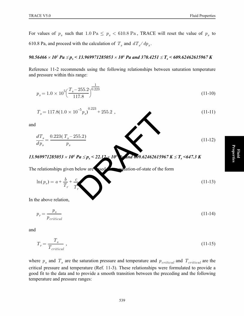
TRACE V5.0 Fluid Properties FOOBAR1234FOOBAR1234FOOBAR1234
Fluid Properties
For values of such that , TRACE will reset the value of to
610.8 Pa, and proceed with the calculation of and .
90.56466 × 10³ Pa ≤ ps < 13.969971285053 × 10⁶ Pa and 370.4251 ≤ Ts < 609.62462615967 K
Reference 11-2 recommends using the following relationships between saturation temperatureand pressure within this range:
(11-10)
, (11-11)
and
(11-12)
13.969971285053 × 10⁶ Pa ≤ ps < 22.12 × 10⁶ Pa and 609.62462615967 K ≤ Ts <647.3 K
The relationships given below are based on an equation-of-state of the form
(11-13)
In the above relation,
(11-14)
and
, (11-15)
where and are the saturation pressure and temperature and and are thecritical pressure and temperature (Ref. 11-3). These relationships were formulated to provide agood fit to the data and to provide a smooth transition between the preceding and the followingtemperature and pressure ranges:
ps 1.0 Pa ps 610.8 Pa<≤ ps
Ts Tsd psd⁄
ps 1.0 105×Ts 255.2–
117.8--------------------------⎝ ⎠
⎛ ⎞1
0.223-------------
=
Ts 117.8 1.0 10 5– ps×( )0.223
255.2+=
psddTs 0.223 Ts 255.2–( )
ps---------------------------------------------=
pr( )ln a bTr------ c
Tr2
------+ +=
prps
pcritical------------------=
TrTs
Tcritical--------------------=
ps Ts pcritical Tcritical
DRAFT
539
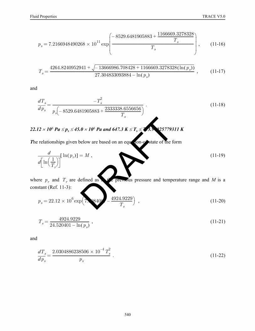
Fluid Properties TRACE V5.0
, (11-16)
, (11-17)
and
. (11-18)
22.12 × 10⁶ Pa ≤ ps ≤ 45.0 × 10⁶ Pa and 647.3 K ≤ Ts ≤ 713.94025779311 K
The relationships given below are based on an equation-of-state of the form
, (11-19)
where and are defined as in the previous pressure and temperature range and M is aconstant (Ref. 11-3):
, (11-20)
, (11-21)
and
. (11-22)
ps 7.2166948490268 1011×8529.6481905883– 1166669.3278328
Ts-------------------------------------------+
Ts--------------------------------------------------------------------------------------------------
⎝ ⎠⎜ ⎟⎜ ⎟⎜ ⎟⎛ ⎞
exp=
Ts4264.8240952941 13666986.708428– 1166669.3278328 ps( )ln( )++
27.304833093884 ps( )ln–-----------------------------------------------------------------------------------------------------------------------------------------------------------------------------=
psddTs Ts
2–
ps 8529.6481905883– 2333338.6556656Ts
-------------------------------------------+⎝ ⎠⎛ ⎞
-------------------------------------------------------------------------------------------------------------=
1Tr------⎝ ⎠
⎛ ⎞lnd
d pr( )ln[ ] M=
pr Tr
ps 22.12 106 7.6084087 4924.9229Ts
-------------------------–⎝ ⎠⎛ ⎞exp×=
Ts4924.9229
24.520401 ps( )ln–-----------------------------------------------=
psddTs 2.0304886238506 10 4– Ts
2×ps
---------------------------------------------------------------------=
DRAFT
540
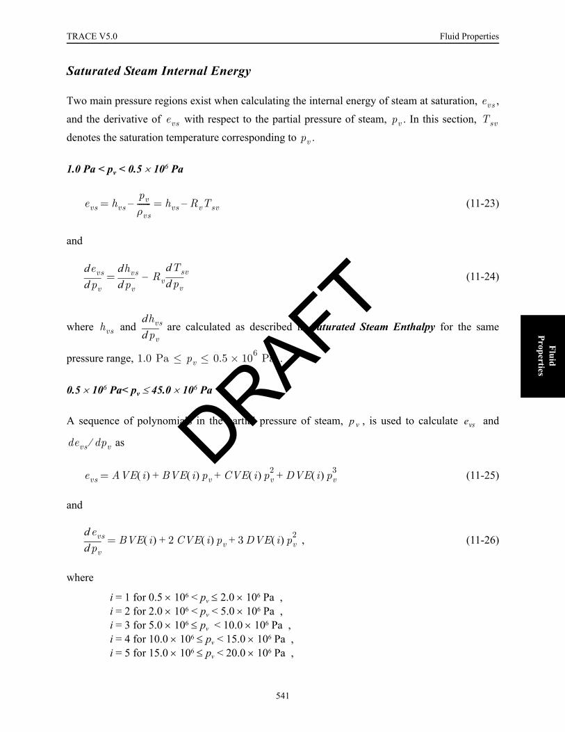
TRACE V5.0 Fluid Properties FOOBAR1234FOOBAR1234FOOBAR1234
Fluid Properties
Saturated Steam Internal Energy
Two main pressure regions exist when calculating the internal energy of steam at saturation, ,
and the derivative of with respect to the partial pressure of steam, . In this section,
denotes the saturation temperature corresponding to .
1.0 Pa < pv < 0.5 × 10⁶ Pa
(11-23)
and
(11-24)
where and are calculated as described in Saturated Steam Enthalpy for the same
pressure range, .
0.5 × 10⁶ Pa< pv ≤ 45.0 × 10⁶ Pa
A sequence of polynomials in the partial pressure of steam, , is used to calculate and
as
(11-25)
and
, (11-26)
where
i = 1 for 0.5 × 10⁶ < pv ≤ 2.0 × 10⁶ Pa ,i = 2 for 2.0 × 10⁶ < pv < 5.0 × 10⁶ Pa ,i = 3 for 5.0 × 10⁶ ≤ pv < 10.0 × 10⁶ Pa ,i = 4 for 10.0 × 10⁶ ≤ pv < 15.0 × 10⁶ Pa ,i = 5 for 15.0 × 10⁶ ≤ pv < 20.0 × 10⁶ Pa ,
evs
evs pv Tsv
pv
evs hvspvρvs-------– hvs RvTsv–= =
pvddevs
pvddhvs Rv pvd
dTsv–=
hvs pvddhvs
1.0 Pa pv 0.5 106 Pa×≤ ≤
p v evs
devs dpv⁄
evs AVE i( ) BVE i( ) pv CVE i( ) pv2 DVE i( ) pv
3+ + +=
pvddevs BVE i( ) 2 CVE i( ) pv 3 DVE i( ) pv
2+ +=
DRAFT
541
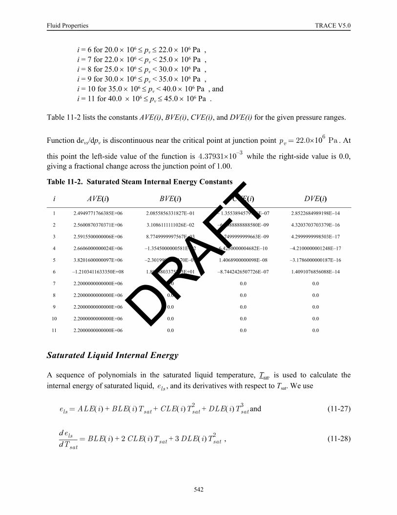
Fluid Properties TRACE V5.0
i = 6 for 20.0 × 10⁶ ≤ pv ≤ 22.0 × 10⁶ Pa ,i = 7 for 22.0 × 10⁶ < pv < 25.0 × 10⁶ Pa ,i = 8 for 25.0 × 10⁶ ≤ pv < 30.0 × 10⁶ Pa ,i = 9 for 30.0 × 10⁶ ≤ pv < 35.0 × 10⁶ Pa ,i = 10 for 35.0 × 10⁶ ≤ pv < 40.0 × 10⁶ Pa , andi = 11 for 40.0 × 10⁶ ≤ pv ≤ 45.0 × 10⁶ Pa .
Table 11-2 lists the constants AVE(i), BVE(i), CVE(i), and DVE(i) for the given pressure ranges.
Function devs/dpv is discontinuous near the critical point at junction point . At
this point the left-side value of the function is while the right-side value is 0.0,giving a fractional change across the junction point of 1.00.
Saturated Liquid Internal Energy
A sequence of polynomials in the saturated liquid temperature, Tsat, is used to calculate theinternal energy of saturated liquid, , and its derivatives with respect to Tsat. We use
and (11-27)
, (11-28)
Table 11-2. Saturated Steam Internal Energy Constants
i AVE(i) BVE(i) CVE(i) DVE(i)
1 2.4949771766385E+06 2.0855856331827E–01 – 1.3553894579716E–07 2.8522684989198E–14
2 2.5600870370371E+06 3.1086111111026E–02 –6.8988888888580E–09 4.3203703703379E–16
3 2.5915500000006E+06 8.7749999997567E–03 –1.7499999999663E–09 4.2999999998503E–17
4 2.6606000000024E+06 –1.3545000000581E–02 6.4250000004682E–10 –4.2100000001248E–17
5 3.8201600000097E+06 –2.3019900000170E–01 1.4068900000098E–08 –3.1786000000187E–16
6 –1.2103411633350E+08 1.8018803375785E+01 –8.7442426507726E–07 1.4091076856088E–14
7 2.2000000000000E+06 0.0 0.0 0.0
8 2.2000000000000E+06 0.0 0.0 0.0
9 2.2000000000000E+06 0.0 0.0 0.0
10 2.2000000000000E+06 0.0 0.0 0.0
11 2.2000000000000E+06 0.0 0.0 0.0
pv 22.0 6×10 Pa=
4.37931 3–×10
els
els ALE i( ) BLE i( )Tsat CLE i( )Tsat2 DLE i( )Tsat
3+ + +=
Tsatddels BLE i( ) 2 CLE i( )Tsat 3 DLE i( )Tsat
2+ +=
DRAFT
542

TRACE V5.0 Fluid Properties FOOBAR1234FOOBAR1234FOOBAR1234
Fluid Properties
where
i = 1 for 273.15 ≤ Tsat < 423.15 K ,i = 2 for 423.15 ≤ Tsat < 473.15 K ,i = 3 for 473.15 ≤ Tsat < 523.15 K ,i = 4 for 523.15 ≤ Tsat < 573.15 K ,i = 5 for 573.15 ≤ Tsat < 623.15 K ,i = 6 for 623.15 ≤ Tsat ≤ 645.15 K ,i = 7 for 645.15 < Tsat < 673.15 K , andi = 8 for 673.15 ≤ Tsat ≤ 713.94025779311 K .
Table 11-3 lists the constants ALE(i), BLE(i), CLE(i), and DLE(i) for the given temperatureranges.
Saturated Steam Enthalpy
Two main pressure regions exist when the enthalpy of steam at saturation is calculated. in
this section denotes the saturation temperature corresponding to the partial pressure of steam, .
1.0 Pa ≤ pv ≤ 0.5 × 10⁶ Pa
Within this pressure region, the enthalpy of saturated steam at temperature is approximatedas the sum of the enthalpy of saturated liquid water at the reference temperature of 273.15 K, plusthe enthalpy necessary to raise the saturated liquid water temperature from 273.15 K to , plus
the latent heat of vaporization needed to convert saturated liquid water at to saturated steam
at . If we define the enthalpy of saturated water at 273.16 K to be exactly zero, this gives
, (11-29)
Table 11-3. Saturated Liquid Internal Energy Constants
i ALE(i) BLE(i) CLE(i) DLE(i)
1 –1.1436668993222E+06 4.1868000000000E+03 0. 0.
2 8.0957542810383E+06 –5.7008855264640E+04 1.3443632119671E+02 –9.7879669155946E–02
3 –1.9373932457007E+06 9.7492797103351E+03 –1.3299615999876E+0l 1.0879999999922E–02
4 –5.3245827703670E+06 2.9179372045334E+04 –5.0452192000967E+0l 3.4560000000583E–02
5 –6.3583523639930E+07 3.2873715263424E+05 –5.6371182000208E+02 3.2760000000116E–01
6 –6.6239163195929E+09 3.1605562257270E+07 –5.0263730855532E+04 2.6650075114186E+01
7 –5.4759091078157E+09 2.4635618770681E+07 –3.6931079506707E+04 1.8454719393083E+01
8 –7.1536399439453E+07 3.0560801674842E+05 –4.2424553999630E+02 1.9719999999823E–01
Tsv
pv
Tsv
Tsv
Tsv
Tsv
hvs 4186.8 273.15 273.16–( ) 4186.8 Tsv 273.15–( ) hlvs+ +=
DRAFT
543
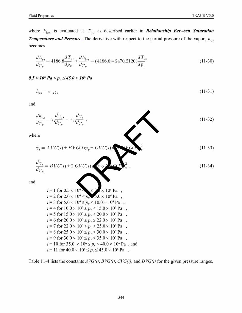
Fluid Properties TRACE V5.0
where is evaluated at as described earlier in Relationship Between Saturation
Temperature and Pressure. The derivative with respect to the partial pressure of the vapor, ,becomes
(11-30)
0.5 × 10⁶ Pa < pv ≤ 45.0 × 10⁶ Pa
(11-31)
and
, (11-32)
where
, (11-33)
, (11-34)
and
i = 1 for 0.5 × 10⁶ < pv ≤ 2.0 × 10⁶ Pa ,i = 2 for 2.0 × 10⁶ < pv < 5.0 × 10⁶ Pa ,i = 3 for 5.0 × 10⁶ ≤ pv < 10.0 × 10⁶ Pa ,i = 4 for 10.0 × 10⁶ ≤ pv < 15.0 × 10⁶ Pa ,i = 5 for 15.0 × 10⁶ ≤ pv < 20.0 × 10⁶ Pa ,i = 6 for 20.0 × 10⁶ ≤ pv ≤ 22.0 × 10⁶ Pa ,i = 7 for 22.0 × 10⁶ < pv < 25.0 × 10⁶ Pa ,i = 8 for 25.0 × 10⁶ ≤ pv < 30.0 × 10⁶ Pa ,i = 9 for 30.0 × 10⁶ ≤ pv < 35.0 × 10⁶ Pa ,i = 10 for 35.0 × 10⁶ ≤ pv < 40.0 × 10⁶ Pa , andi = 11 for 40.0 × 10⁶ ≤ pv ≤ 45.0 × 10⁶ Pa .
Table 11-4 lists the constants AVG(i), BVG(i), CVG(i), and DVG(i) for the given pressure ranges.
hlvs Tsv
pv
pvddhvs 4186.8
pvddTsv
pvddhlvs+ 4186.8 2470.2120–( )
pvddTsv= =
hvs evsγs=
pvddhvs γs pvd
d evs evs pvddγs+=
γs AVG i( ) BVG i( )pv CVG i( )pv2 DVG i( )pv
3+ + +=
pvddγs BVG i( ) 2 CVG i( ) pv 3 DVG i( ) pv
2+ +=
DRAFT
544

TRACE V5.0 Fluid Properties FOOBAR1234FOOBAR1234FOOBAR1234
Fluid Properties
Functions hvs/dpv and dγs/dpv are both discontinuous near the critical point at junction point
. At this point, the left-side value of hvs/dpv is and the right-
side value for a fractional change here of 1.0011. The left-side value of
is and the right-side value is giving a fractional change at thisjunction point of .
Saturated Liquid Enthalpy
From the definition of enthalpy,
(11-35)
and
, (11-36)
where and its derivative are evaluated as shown in Saturated Liquid Internal Energy, and
where and its derivatives are evaluated using the equations in Density with equal to Tsat.
Table 11-4. Saturated Steam Enthalpy Constants
i AVG(i) BVG(i) CVG(i) DVG(i)
1 1.0666845123419E+00 2.8310838172462E–08 –2.1151097428905E–14 4.7404001285964E–21
2 1.0735412407407E+00 2.6518055555551E–09 –6.3461111111128E–16 3.9824074074117E–23
3 1.0777730000000E+00 –2.4300000008021E–11 –7.1979999998378E–17 4.8799999990422E–25
4 1.0851130000007E+00 –1.9307000001824E–09 8.9100000014826E–17 –3.8960000003946E–24
5 1.1639800000015E+00 –1.6338350000254E–08 9.5856000001448E–16 –2.1194000000274E–23
6 3.8898867259868E+00 –3.8595945559811E–07 1.7476370114910E–14 –2.6377008249858E–22
7 2.7168710524682E+00 –2.2832718294604E–07 1.0417331983836E–14 –1.5842822199773E–22
8 3.9749829999964E+00 –3.0657099999960E–07 1.0637899999985E–14 –1.2257999999981E–22
9 1.2946929999997E+00 –2.4834999999979E–08 7.8979999999944E–16 –8.0799999999948E–24
10 1.0590519999963E+00 –2.4615999996941E–09 8.8399999991573E–17 –8.0799999992269E–25
11 1.1430199999838E+00 –7.7095999988588E–09 1.9335999997331E–16 –1.4639999997924E–24
pv 22.0 106 Pa×= 4.6073 3–×10
5.1790– 6–×10 γsd pvd⁄
6.6694 12–×10 2.3541– 2–×101.3530
hls elspρls------+=
pddhls
Tsatddels
pddTsat 1
ρls------ p
ρls2
------p∂
∂ρls⎝ ⎠⎛ ⎞
Tsat Tsat∂∂ρls
⎝ ⎠⎜ ⎟⎛ ⎞
ppd
dTsat+–+=
els
ρls Tl
DRAFT
545
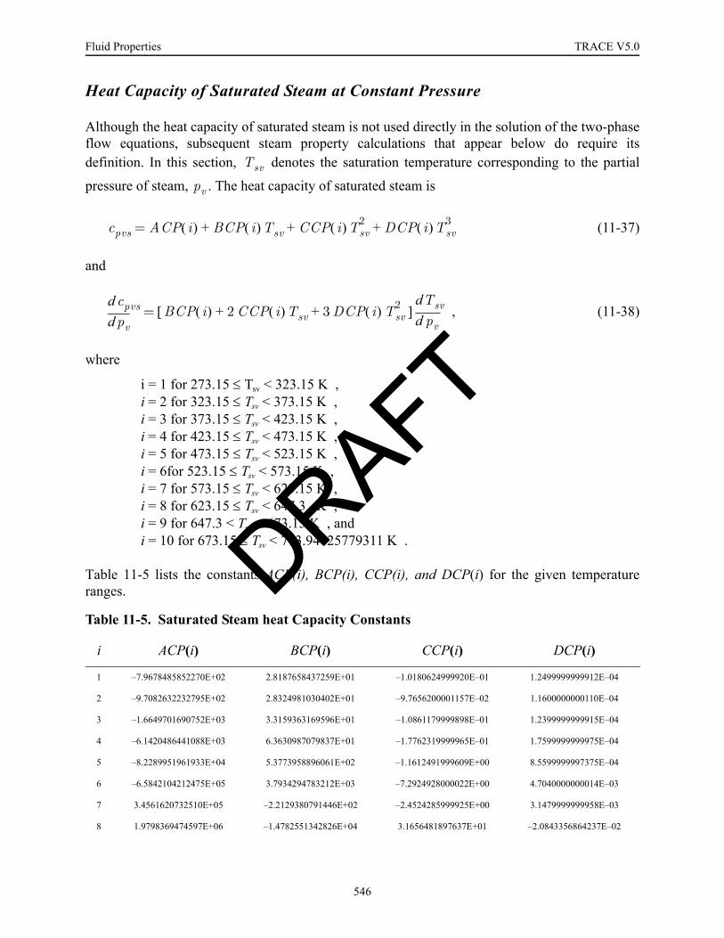
Fluid Properties TRACE V5.0
Heat Capacity of Saturated Steam at Constant Pressure
Although the heat capacity of saturated steam is not used directly in the solution of the two-phaseflow equations, subsequent steam property calculations that appear below do require itsdefinition. In this section, denotes the saturation temperature corresponding to the partial
pressure of steam, . The heat capacity of saturated steam is
(11-37)
and
, (11-38)
where
i = 1 for 273.15 ≤ Tsv < 323.15 K ,i = 2 for 323.15 ≤ Tsv < 373.15 K ,i = 3 for 373.15 ≤ Tsv < 423.15 K ,i = 4 for 423.15 ≤ Tsv < 473.15 K ,i = 5 for 473.15 ≤ Tsv < 523.15 K ,i = 6for 523.15 ≤ Tsv < 573.15 K ,i = 7 for 573.15 ≤ Tsv < 623.15 K ,i = 8 for 623.15 ≤ Tsv < 647.3 K ,i = 9 for 647.3 < Tsv < 673.15 K , andi = 10 for 673.15 ≤ Tsv < 713.94025779311 K .
Table 11-5 lists the constants ACP(i), BCP(i), CCP(i), and DCP(i) for the given temperatureranges.
Table 11-5. Saturated Steam heat Capacity Constants
i ACP(i) BCP(i) CCP(i) DCP(i)
1 –7.9678485852270E+02 2.8187658437259E+01 –1.0180624999920E–01 1.2499999999912E–04
2 –9.7082632232795E+02 2.8324981030402E+01 –9.7656200001157E–02 1.1600000000110E–04
3 –1.6649701690752E+03 3.3159363169596E+01 –1.0861179999898E–01 1.2399999999915E–04
4 –6.1420486441088E+03 6.3630987079837E+01 –1.7762319999965E–01 1.7599999999975E–04
5 –8.2289951961933E+04 5.3773958896061E+02 –1.1612491999609E+00 8.5599999997375E–04
6 –6.5842104212475E+05 3.7934294783212E+03 –7.2924928000022E+00 4.7040000000014E–03
7 3.4561620732510E+05 –2.2129380791446E+02 –2.4524285999925E+00 3.1479999999958E–03
8 1.9798369474597E+06 –1.4782551342826E+04 3.1656481897637E+01 –2.0843356864237E–02
Tsv
pv
cpvs ACP i( ) BCP i( )Tsv CCP i( )Tsv2 DCP i( )Tsv
3+ + +=
pvddcpvs BCP i( ) 2 CCP i( )Tsv 3 DCP i( ) Tsv
2+ +[ ]pvd
dTsv=
DRAFT
546

TRACE V5.0 Fluid Properties FOOBAR1234FOOBAR1234FOOBAR1234
Fluid Properties
Liquid Properties
Internal Energy
Given a liquid at some temperature, , and some pressure, p, the liquid internal energyassociated with that state is calculated by beginning with the internal energy of the saturatedliquid state described by and PSL, where PSL is the saturation pressure corresponding to ,
and adding an additional term that represents the change in internal energy from the state ( ,
PSL) to the state ( , p) That is,
. (11-39)
The additional term, ELP, which represents the change in energy required to move along theisotherm at between two different pressure values, namely PSL and p, is represented as
, (11-40)
where
(11-41)
Therefore, the partial derivative with respect to of the internal energy is calculated as
(11-42)
where
9 –9.6249385211359E+07 4.3633668884423E+05 –6.5887615106930E+02 3.3146147264269E–01
10 –1.1074934463333E+07 4.8073794630970E+04 –6.9212173247881E+0l 3.3091693999800E–02
Table 11-5. Saturated Steam heat Capacity Constants
i ACP(i) BCP(i) CCP(i) DCP(i)
Tl
Tl Tl
Tl
Tl
el Tl, p( ) els Tl, PSL( ) ELP+=
Tl
ELP p PSL–( )p∂
∂ el⎝ ⎠⎛ ⎞
Tl=
p∂∂ el
⎝ ⎠⎛ ⎞ 8.329595 10 4–× 1 e
1.450382 10 6– PSL×–– 2.245825 10 17–× PSL2–=
Tl
Tl∂∂el
⎝ ⎠⎜ ⎟⎛ ⎞
p Tsatdd els ERT+=
DRAFT
547

Fluid Properties TRACE V5.0
and dels/dTsat is calculated as in Saturated Liquid Internal Energy
Density
Initial Calculation
Given the pressure p and temperature of liquid water, Tait’s equation-of-state in the form
(11-43)
is used to determine the liquid density and its partial derivatives, where is the specific volumeof the liquid. The constant is quoted in work by Richardson, Arens, and Haverson (Ref. 11-4)
to be 7.146. The terms and are third-order polynomials of liquid temperaturefitted to steam-table data, such that
(11-44)
and
, (11-45)
where
i = 1 for 273.15 ≤ Tl < 373.15 K ,i = 2 for 373.15 ≤ Tl < 473.15 K ,i = 3 for 473.15 ≤ Tl < 573.15 K ,i = 4 for 573.15 ≤ Tl < 603.15 K ,i = 5 for 603.15 ≤ Tl < 613.15 K ,i = 6 for 613.15 ≤ Tl < 623.15 K ,i = 7 for 623.15 ≤ Tl < 633.15 K ,
ERTTl∂∂ ELP( )
p
= 8.329595 4–×10 1– e 1.450382– 6–×10 PSL 1 1.450382 6–×10 p PSL–( )+[ ]×+[ ]–
2.245825 17–×10 2p PSL 3PSL2–·( )–
⎩
⎭
⎨
⎬
⎧
⎫Tldd PSL( )
=
Tl
v 0 Tl,( ) v p Tl,( )–
v 0 Tl,( )------------------------------------------------ 1
n--- 1 p
B Tl( )---------------+ln=
vn
v 0 Tl,( ) B Tl( )
v 0 Tl,( ) AVO i( ) BVO i( ) Tl CVO i( ) Tl2 DVO i( ) Tl
3+ + +=
B Tl( ) AFN i( ) BFN i( ) Tl CFN i( ) Tl2 DFN i( ) Tl
3+ + +=
DRAFT
548
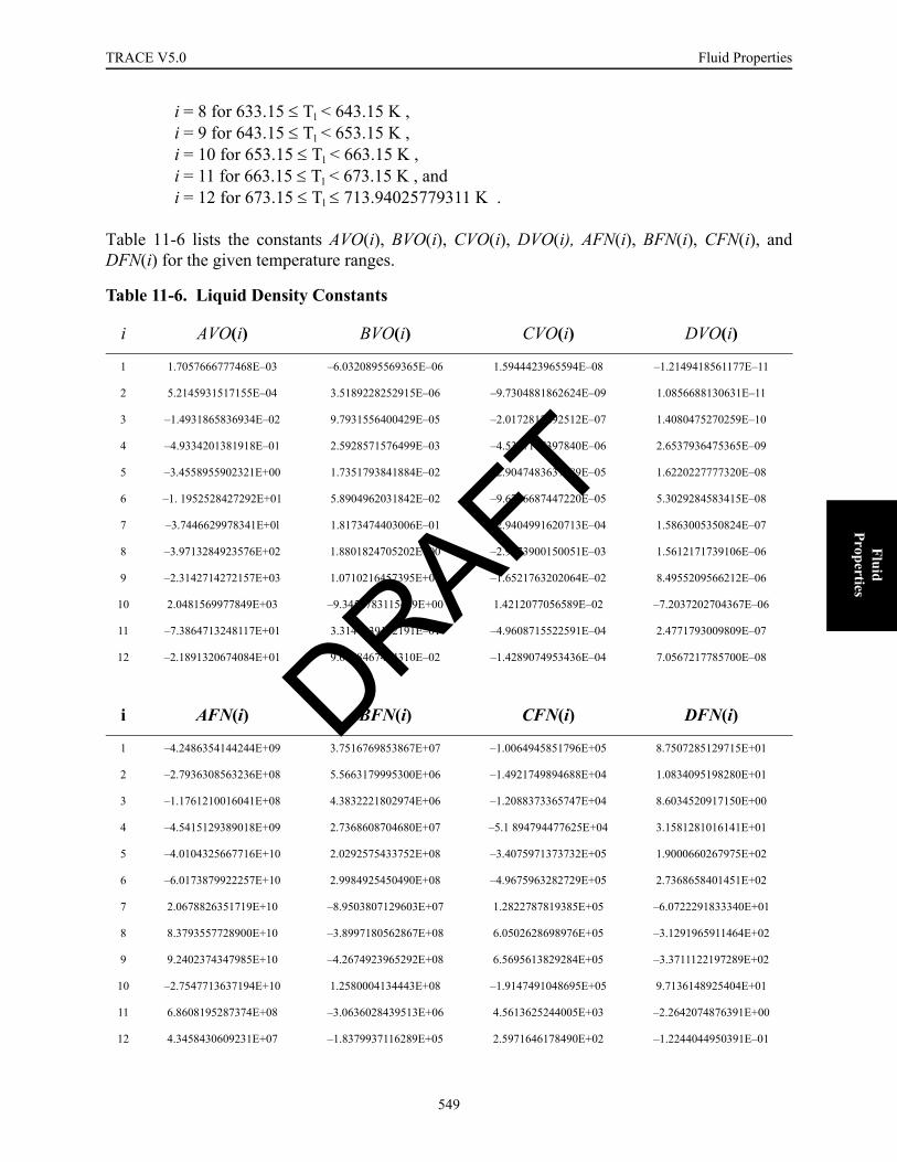
TRACE V5.0 Fluid Properties FOOBAR1234FOOBAR1234FOOBAR1234
Fluid Properties
i = 8 for 633.15 ≤ Tl < 643.15 K ,i = 9 for 643.15 ≤ Tl < 653.15 K ,i = 10 for 653.15 ≤ Tl < 663.15 K ,i = 11 for 663.15 ≤ Tl < 673.15 K , andi = 12 for 673.15 ≤ Tl ≤ 713.94025779311 K .
Table 11-6 lists the constants AVO(i), BVO(i), CVO(i), DVO(i), AFN(i), BFN(i), CFN(i), andDFN(i) for the given temperature ranges.
Table 11-6. Liquid Density Constants
i AVO(i) BVO(i) CVO(i) DVO(i)
1 1.7057666777468E–03 –6.0320895569365E–06 1.5944423965594E–08 –1.2149418561177E–11
2 5.2145931517155E–04 3.5189228252915E–06 –9.7304881862624E–09 1.0856688130631E–11
3 –1.4931865836934E–02 9.7931556400429E–05 –2.0172817692512E–07 1.4080475270259E–10
4 –4.9334201381918E–01 2.5928571576499E–03 –4.5387107397840E–06 2.6537936475365E–09
5 –3.4558955902321E+00 1.7351793841884E–02 –2.9047483637289E–05 1.6220227777320E–08
6 –1. 1952528427292E+01 5.8904962031842E–02 –9.6786687447220E–05 5.3029284583415E–08
7 –3.7446629978341E+0l 1.8173474403006E–01 –2.9404991620713E–04 1.5863005350824E–07
8 –3.9713284923576E+02 1.8801824705202E+00 –2.9673900150051E–03 1.5612171739106E–06
9 –2.3142714272157E+03 1.0710216457395E+01 –1.6521763202064E–02 8.4955209566212E–06
10 2.0481569977849E+03 –9.3452783115489E+00 1.4212077056589E–02 –7.2037202704367E–06
11 –7.3864713248117E+01 3.3144939132191E–01 –4.9608715522591E–04 2.4771793009809E–07
12 –2.1891320674084E+01 9.6758467414310E–02 –1.4289074953436E–04 7.0567217785700E–08
i AFN(i) BFN(i) CFN(i) DFN(i)
1 –4.2486354144244E+09 3.7516769853867E+07 –1.0064945851796E+05 8.7507285129715E+01
2 –2.7936308563236E+08 5.5663179995300E+06 –1.4921749894688E+04 1.0834095198280E+01
3 –1.1761210016041E+08 4.3832221802974E+06 –1.2088373365747E+04 8.6034520917150E+00
4 –4.5415129389018E+09 2.7368608704680E+07 –5.1 894794477625E+04 3.1581281016141E+01
5 –4.0104325667716E+10 2.0292575433752E+08 –3.4075971373732E+05 1.9000660267975E+02
6 –6.0173879922257E+10 2.9984925450490E+08 –4.9675963282729E+05 2.7368658401451E+02
7 2.0678826351719E+10 –8.9503807129603E+07 1.2822787819385E+05 –6.0722291833340E+01
8 8.3793557728900E+10 –3.8997180562867E+08 6.0502628698976E+05 –3.1291965911464E+02
9 9.2402374347985E+10 –4.2674923965292E+08 6.5695613829284E+05 –3.3711122197289E+02
10 –2.7547713637194E+10 1.2580004134443E+08 –1.9147491048695E+05 9.7136148925404E+01
11 6.8608195287374E+08 –3.0636028439513E+06 4.5613625244005E+03 –2.2642074876391E+00
12 4.3458430609231E+07 –1.8379937116289E+05 2.5971646178490E+02 –1.2244044950391E–01
DRAFT
549
Fluid Properties TRACE V5.0
This allows the density, to be calculated as
(11-46)
Therefore,
(11-47)
and
(11-48)
where
(11-49)
and
(11-50)
The polynomial constants for and are the same as for and andare given in Table 11-6
Residual Void Correction1
After evaluation in the above section, and its derivatives are corrected to reflect a residual voidfraction. In the following, the values calculated above are denoted by a tilde (˜).
p ≥ 4.0 × 10⁵ Pa
, (11-51)
1. This artificial compressibility of liquid is presently turned off in the code. It can be turned on by setting the flag NOAC to 0 in subroutine RHOLIQ if it is needed.
ρl
ρl1
v 0 Tl,( ) 1.0 17.146------------- 1.0 p
B Tl( )---------------+ln–
⎩ ⎭⎨ ⎬⎧ ⎫
----------------------------------------------------------------------------------------------------=
p∂∂ρl
⎝ ⎠⎛ ⎞
Tl
ρl2 v 0 Tl,( )
7.146 p B Tl( )+[ ]--------------------------------------------=
Tl∂∂ρl
⎝ ⎠⎜ ⎟⎛ ⎞
pρl
v′ 0 Tl,( )
v 0 Tl,( )-----------------------
⎝ ⎠⎜ ⎟⎛ ⎞
– B′ Tl( ) pB Tl( )---------------⎝ ⎠
⎛ ⎞p∂
∂ρl⎝ ⎠⎛ ⎞
Tl–=
v′ 0 Tl,( ) BVO i( ) 2 CVO i( ) Tl 3 DVO i( ) Tl2+ +=
B′ Tl( ) BFN i( ) 2 CFN i( ) Tl 3 DFN i( ) Tl2+ +=
v′ 0 Tl,( ) B′ Tl( ) v 0 Tl,( ) B Tl( )
ρl
Tl∂∂ρl
⎝ ⎠⎜ ⎟⎛ ⎞
p1 1000
p------------–⎝ ⎠
⎛ ⎞Tl∂
∂ ρl⎝ ⎠⎛ ⎞
p=
DRAFT
550
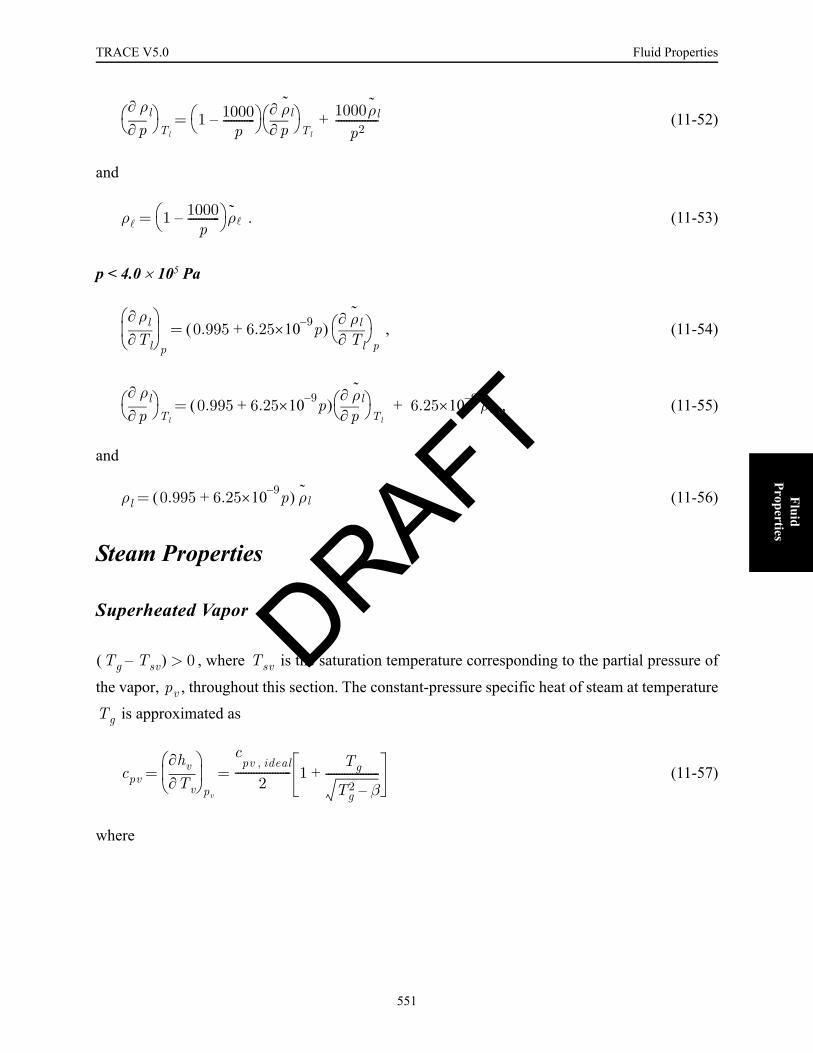
TRACE V5.0 Fluid Properties FOOBAR1234FOOBAR1234FOOBAR1234
Fluid Properties
(11-52)
and
. (11-53)
p < 4.0 × 10⁵ Pa
, (11-54)
, (11-55)
and
(11-56)
Steam Properties
Superheated Vapor
, where is the saturation temperature corresponding to the partial pressure of
the vapor, , throughout this section. The constant-pressure specific heat of steam at temperature
is approximated as
(11-57)
where
p∂∂ ρl
⎝ ⎠⎛ ⎞
Tl1 1000
p------------–⎝ ⎠
⎛ ⎞p∂
∂ ρl⎝ ⎠⎛ ⎞
Tl
1000ρl
p2----------------+=
ρl 1 1000p
------------–⎝ ⎠⎛ ⎞ ρl=
Tl∂∂ρl
⎝ ⎠⎜ ⎟⎛ ⎞
p0.995 6.25 9–×10 p+( )
Tl∂∂ ρl
⎝ ⎠⎛ ⎞
p=
p∂∂ ρl
⎝ ⎠⎛ ⎞
Tl0.995 6.25 9–×10 p+( )
p∂∂ ρl
⎝ ⎠⎛ ⎞
Tl6.25 9–×10 ρl+=
ρl 0.995 6.25 9–×10 p+( ) ρl=
Tg Tsv–( ) 0> Tsv
pv
Tg
cpv Tv∂∂hv
⎝ ⎠⎜ ⎟⎛ ⎞
pv
cpv ideal,
2--------------------- 1
Tg
Tg2 β–
--------------------+= =
DRAFT
551
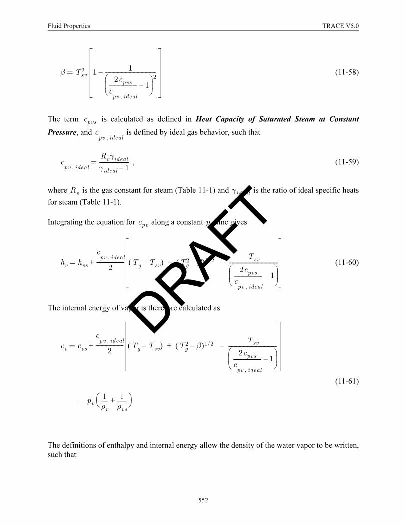
Fluid Properties TRACE V5.0
(11-58)
The term is calculated as defined in Heat Capacity of Saturated Steam at Constant
Pressure, and is defined by ideal gas behavior, such that
, (11-59)
where is the gas constant for steam (Table 11-1) and is the ratio of ideal specific heatsfor steam (Table 11-1).
Integrating the equation for along a constant line gives
(11-60)
The internal energy of vapor is therefore calculated as
(11-61)
The definitions of enthalpy and internal energy allow the density of the water vapor to be written,such that
β Tsv2 1 1
2cpvscpv ideal,
--------------------- 1–⎝ ⎠⎜ ⎟⎛ ⎞ 2--------------------------------------–=
cpvs
cpv ideal,
cpv ideal,
Rvγidealγideal 1–----------------------=
Rv γideal
cpv pv
hv hvs
cpv ideal,
2--------------------- Tg Tsv–( ) Tg
2 β–( )1 2/ Tsv
2cpvscpv ideal,
--------------------- 1–⎝ ⎠⎜ ⎟⎛ ⎞------------------------------------–++=
ev evs
cpv ideal,
2--------------------- Tg Tsv–( ) Tg
2 β–( )1 2/ Tsv
2cpvscpv ideal,
--------------------- 1–⎝ ⎠⎜ ⎟⎛ ⎞------------------------------------–+
pv1ρv----- 1
ρvs-------+⎝ ⎠
⎛ ⎞–
+=DRAFT
552

TRACE V5.0 Fluid Properties FOOBAR1234FOOBAR1234FOOBAR1234
Fluid Properties
(11-62)
where is defined in Table 11-1
Internal Energy
Substitution of and , as defined by the preceding equation, into the equation for the internalenergy of the vapor gives the following equations.
For
(11-63)
where again is the constant-volume specific heat for steam, as defined by ideal gas
behavior (Table 11-1). Therefore,
(11-64)
and
, (11-65)
where
ρvpv
hv ev–----------------
pv
hvs cpv ideal,
Tg Tsv–( )+[ ] evs cvv ideal,
Tg Tsv–( )+[ ]–------------------------------------------------------------------------------------------------------------------------------------------
= pv
hvs evs–( ) γideal 1–( ) ev evs–( )+----------------------------------------------------------------------------------
= =
cvv ideal,
ρv ρvs
pv 1.9 7×10 Pa≤
ev evs
cvv ideal,
2--------------------- Tg Tsv–( ) Tg
2 β–( )1 2/ Tsv
2cpvscpv ideal,
--------------------- 1–⎝ ⎠⎜ ⎟⎛ ⎞------------------------------------–++=
cvv ideal,
Tg∂∂ ev
⎝ ⎠⎜ ⎟⎛ ⎞
pv
cvv ideal,
1 βκ2------–⎝ ⎠
⎛ ⎞---------------------=
pv∂∂ ev
⎝ ⎠⎜ ⎟⎛ ⎞
Tg
12---
Tg∂∂ ev
⎝ ⎠⎜ ⎟⎛ ⎞
pv
1 βκ2------–⎝ ⎠
⎛ ⎞κp′1κ---
pvddβ+–=
DRAFT
553

Fluid Properties TRACE V5.0
, (11-66)
and
(11-67)
and
(11-68)
For ,
, (11-69)
, (11-70)
and
κ 2c
vv ideal,
--------------------- ev evs–( ) Tsv 1 12cpvs
cpv ideal,-------------------- 1–-----------------------------++=
κp′ pv∂∂κ
⎝ ⎠⎛ ⎞
Tg
2c
vv ideal,
---------------------pvd
d evs– 1 12cpvs
cpv ideal,
--------------------- 1–⎝ ⎠⎜ ⎟⎛ ⎞------------------------------------+
pvddTsv
2c
pv ideal,
---------------------Tsv
2cpvscpv ideal,
--------------------- 1–⎝ ⎠⎜ ⎟⎛ ⎞ 2----------------------------------------
pvddcpvs
–
+= =
pvddβ 2
Tsv-------- β
pvddTsv 2
cpv ideal,
---------------------Tsv
2cpvsc
pv ideal,
--------------------- 1–⎝ ⎠⎜ ⎟⎛ ⎞------------------------------------
pvddcpvs+
⎩ ⎭⎪ ⎪⎪ ⎪⎨ ⎬⎪ ⎪⎪ ⎪⎧ ⎫
=
pv 2.0 7×10 Pa≥
ev evscpv, ideal
2γs-------------------
Tg Tsv–( ) Tg2 β–( )
1 2⁄Tsv–+
2cpvscpv, ideal------------------- 1–⎝ ⎠
⎛ ⎞----------------------------------------------------------------------------+=
Tg∂∂ ev
⎝ ⎠⎜ ⎟⎛ ⎞
pv
cpv, ideal2γs
------------------- 1Tg
Tg2 β–( )
1 2⁄----------------------------+
⎝ ⎠⎜ ⎟⎜ ⎟⎛ ⎞
=
DRAFT
554

TRACE V5.0 Fluid Properties FOOBAR1234FOOBAR1234FOOBAR1234
Fluid Properties
(11-71)
where
(11-72)
For the values of and its derivatives are calculated byinterpolating between the values of the two curve fits.
Density
If the vapor density is calculated as
(11-73)
Therefore,
, (11-74)
and
(11-75)
where
pv∂∂ ev
⎝ ⎠⎜ ⎟⎛ ⎞
Tgpvd
devs ev evs–γs
------------------pvd
dγs–c
pv ideal,
2γs---------------------
pvddTsv–
⎝ ⎠⎜ ⎟⎛ ⎞ 1
2---
pvddβ
⎝ ⎠⎛ ⎞ 1
Tg2 β–
--------------------⎝ ⎠⎜ ⎟⎛ ⎞
–
pvddTsv
12cpvs
cpv, ideal------------------- 1–⎝ ⎠
⎛ ⎞----------------------------------
⎝ ⎠⎜ ⎟⎜ ⎟⎜ ⎟⎛ ⎞
2cpv ideal,
---------------------Tsv
2cpvscpv, ideal------------------- 1–⎝ ⎠
⎛ ⎞ 2-------------------------------------
pvddcpvs+·–
·+=
pv∂∂β 2
Tsv-------- β
pvddTsv 2
cpv ideal,
---------------------Tsv
2cpvscpv, ideal------------------- 1–⎝ ⎠
⎛ ⎞------------------------------------
3
pvddcpvs+
⎩ ⎭⎪ ⎪⎨ ⎬⎪ ⎪⎧ ⎫
=
1.9 7×10 Pa pv 2.0 7×10 Pa< < ev
pv 1.9 7×10 Pa≤
ρvρv
γs 1–( )evs γideal 1–( ) ev evs–( )+-----------------------------------------------------------------------------------=
Tg∂∂pv
⎝ ⎠⎜ ⎟⎛ ⎞
pvTg∂
∂ ev
⎝ ⎠⎜ ⎟⎛ ⎞
pv
γideal 1–( )ρvγs 1–( )evs γideal 1–( ) ev evs–( )+
-----------------------------------------------------------------------------------–=
pv∂∂ρv
⎝ ⎠⎜ ⎟⎛ ⎞
Tg
1 ρv–( ) evs pvddγs γs γideal–( )
pvddevs+
1γs 1–( )evs γideal 1–( ) ev evs–( )+
-----------------------------------------------------------------------------------
·⎩
⎭
⎨
⎬
⎧
⎫ev∂
∂ρv
⎝ ⎠⎜ ⎟⎛ ⎞
pvpv∂
∂ev
⎝ ⎠⎜ ⎟⎛ ⎞
Tg
+
=
DRAFT
555

Fluid Properties TRACE V5.0
. (11-76)
If , the vapor density is calculated as
(11-77)
Therefore,
(11-78)
and
(11-79)
where
. (11-80)
If , the vapor density and its derivatives are calculated bylinearly interpolating between the values of the two curve fits.
Minimum and maximum limits are placed on the calculated values of the density, and its partialderivatives. In low-pressure regions where the above equations may predict a negative density,the density and its derivatives are recalculated based on ideal gas behavior. If is less than zero,the vapor density and its derivatives are superseded by
, (11-81)
, (11-82)
ev∂∂ρv
⎝ ⎠⎜ ⎟⎛ ⎞
pv
γideal 1–( )ρvγs 1–( )evs γideal 1–( ) ev evs–( )+
-----------------------------------------------------------------------------------=
pv 2.0 7×10 Pa≥
ρvpv
γs 1–( )ev------------------------=
Tg∂∂pv
⎝ ⎠⎜ ⎟⎛ ⎞
pvev∂
∂ρv
⎝ ⎠⎜ ⎟⎛ ⎞
pvTg∂
∂ev
⎝ ⎠⎜ ⎟⎛ ⎞
pv
=
pv∂∂ρv
⎝ ⎠⎜ ⎟⎛ ⎞
Tg
1 ρvev pvddγs–
⎝ ⎠⎜ ⎟⎛ ⎞ 1
γs 1–( )ev------------------------
ev∂∂ρv
⎝ ⎠⎜ ⎟⎛ ⎞
pvpv∂
∂ev
⎝ ⎠⎜ ⎟⎛ ⎞
Tg
+=
ev∂∂ρv
⎝ ⎠⎜ ⎟⎛ ⎞
pv
ρvev-----–=
1.9 7×10 Pa pv 2.0 7×10 Pa< <
ρv
ρvpv
RvTg-------------=
Tv∂∂ρv
⎝ ⎠⎜ ⎟⎛ ⎞
pv
ρvTg------–=
DRAFT
556

TRACE V5.0 Fluid Properties FOOBAR1234FOOBAR1234FOOBAR1234
Fluid Properties
and
. (11-83)
Near the critical point, it is necessary to impose the following limit on the density ratio when thepressure is less than the critical pressure.
(11-84)
to avoid singularities when calculating certain parameters. If the calculated value of exceeds
the vapor density and its derivatives are superseded by
, (11-85)
, (11-86)
and
(11-87)
For conditions above the critical pressure, is retained.
Enthalpy
The EOS package calculates the enthalpy of the superheated vapor using the definition ofenthalpy, such that
(11-88)
where ev and ρv are calculated from Eqs. (11-63) (or (11-69)) and (11-73) (or (11-77), or (11-81)),respectively.
pv∂∂ρv
⎝ ⎠⎜ ⎟⎛ ⎞
Tg
ρvpg-----–=
ρvρl----- 0.999≤
ρv
0.999ρl
ρv 0.999ρl=
ρv∂
Tg∂----------
⎝ ⎠⎜ ⎟⎛ ⎞
pv
0.999ρl∂
Tl∂---------
⎝ ⎠⎜ ⎟⎛ ⎞
p
=
pv∂∂ρv
⎝ ⎠⎜ ⎟⎛ ⎞
Tg
0.999p∂
∂ρl⎝ ⎠⎛ ⎞
Tl=
ρv
hv evpvρv-----+=
DRAFT
557

Fluid Properties TRACE V5.0
Subcooled Vapor
where refers to the saturation temperature corresponding to the partial
pressure of the vapor, throughout this section.
Internal Energy
, (11-89)
, (11-90)
and
(11-91)
Density
The method used to determine the subcooled vapor density, and its derivatives for all pressure
ranges is identical to the one outlined in the case of superheated vapor for , asgiven by Eq. (11-73).
Enthalpy
TRACE calculates the enthalpy of the subcooled vapor using the definition of enthalpy, such that
, (11-92)
where and are calculated from Eqs. (11-89) and (11-73). respectively.
Noncondensable Gas (Air, Hydrogen, or Helium) Properties
In general, TRACE treats the noncondensable field as an ideal gas. You have the option ofchoosing any of the following gases: air, argon, hydrogen, or helium1, krypton, nitrogen, or
Tg Tsv–( ) 0≤ Tsv
pv
ev evs Tg Tsv–( )cpvsγideal-------------+=
Tg∂∂ ev
⎝ ⎠⎜ ⎟⎛ ⎞
pv
cpvsγideal-------------=
pv∂∂ ev
⎝ ⎠⎜ ⎟⎛ ⎞
Tgpvd
d evs ev evs–cpvs
------------------⎝ ⎠⎛ ⎞
pvddcpvs
Tg∂∂ ev
pvddTsv–+=
pv 1.9 7×10 Pa≤
hv evpvρv-----+=
ev ρv
DRAFT
558

TRACE V5.0 Fluid Properties FOOBAR1234FOOBAR1234FOOBAR1234
Fluid Properties
xenon. TRACE allows you to model either a single species of noncondensable gas or somecombination thereof.
TRACE calculates the thermodynamic properties for the non-condensible gas field with thefollowing correlations:
Internal Energy
The internal energy and its derivatives are given by (see Reference 11-14, pp. 21-22,Eqs. 1.29-1.32, for air and hydrogen and Reference 11-15, p. 247, for helium)
, (11-93)
, (11-94)
and
. (11-95)
The constant-volume specific heat, , is calculated from
, (11-96)
where is the specific heat at constant pressure for noncondensable gases (determined as
described below in the section Constant-Pressure Specific Heat) and is the gas constant forthe noncondensable gas, as determined from
, (11-97)
1. More accurate properties also are available for helium. These optional properties for helium are not dis-cussed here; see Reference 11-18 for complete details. Currently, these properties are only available for light water models (H2O).
ea cvaTg=
ea∂
Tg∂----------
⎝ ⎠⎜ ⎟⎜ ⎟⎛ ⎞
pa
cva=
pa∂∂ ea
⎝ ⎠⎜ ⎟⎛ ⎞
Tg
0.0=
cva
cva cpa Ra–=
cpa
Ra
RaRMa-------=
DRAFT
559

Fluid Properties TRACE V5.0
where is the universal gas constant and is the mass of one mole (molecular weight with
units of kg) of the noncondensible gas. Since and are both constants for a give
noncondensible gas, the values of used by TRACE are provided in Table 11-1.
Density
We use the ideal-gas law for the air, hydrogen, and helium density correlations. Because the ideal-gas law accurately predicts gas behavior for low pressure and high temperature, and TRACEusually deals with this range of pressures and temperatures, we consider the ideal-gas correlationto provide an adequate approximation for the gas densities. The density is calculated according tothe following set of relationships (Ref. 11-16):
, (11-98)
, (11-99)
and
(11-100)
where is the microscopic density, is the noncondensible partial pressure, is the
temperature of the gas, and is the noncondensible gas constant, as defined in the previoussection.
Enthalpy
TRACE calculates the enthalpy of the noncondensable gas, such that
, (11-101)
where and are calculated from Eqs. (11-93) and (11-98) respectively.
R Ma
R Ma
Ra
ρapa
RaTg-------------=
pa∂∂ρa
⎝ ⎠⎜ ⎟⎛ ⎞
Tg
1RaTg-------------=
Tg∂∂ρa
⎝ ⎠⎜ ⎟⎛ ⎞
pa
Ra ρa pa∂∂ρa
⎝ ⎠⎜ ⎟⎛ ⎞
Tg
–=
ρa Pa Tg
Ra
ha eapaρa-----+=
ea ρa
DRAFT
560

TRACE V5.0 Fluid Properties FOOBAR1234FOOBAR1234FOOBAR1234
Fluid Properties
Steam-Gas Mixture Properties
Internal Energy
The EOS package calculates the steam-noncondensible gas mixture internal energy, such that
, (11-102)
where is calculated according to Eq. (11-61) or Eq. (11-89), depending upon whether the
vapor is superheated or subcooled, is calculated according to Eq. (11-93), is the water
vapor density as calculated in Eq. (11-73) or Eq. (11-77), and is the noncondensable-gasdensity as calculated in Eq. (11-98).
Density
The EOS package calculates the steam-noncondensible gas mixture density, such that
, (11-103)
where is the water vapor density as calculated in Eq. (11-73) or Eq. (11-77) and is thenoncondensable-gas density as calculated in Eq. (11-98).
Enthalpy
The EOS package calculates the steam-noncondensible gas mixture enthalpy, such that
, (11-104)
where is calculated according to Eq. (11-102), is calculated according to Eq. (11-103),and p is the total pressure.
Transport PropertiesThe EOS package is used to obtain transport properties for liquid- and vapor-phase water,noncondensable gases, and steam-gas mixtures. The input variables in this case are the saturationtemperature corresponding to the total pressure; the internal energies, densities, and temperatures
emevρv eaρa+ρv ρa+
----------------------------=
ev
ea ρv
ρa
ρm ρv ρa+=
ρv ρa
hmhvρv haρa+ρv ρv+
----------------------------- empρm-------+= =
em ρm
DRAFT
561

Fluid Properties TRACE V5.0
of the liquid and gas phases where the gas is either steam, a noncondensable gas, or a steam-gasmixture; the total pressure; and the partial pressure of the noncondensable gas, if any is present.The output transport variables include the latent heat of vaporization, the constant-pressurespecific heats, viscosities, and thermal conductivities of the liquid and gas phases, and the surfacetension of the liquid.
The polynomial equation fits for the transport properties used in TRACE are described in theremainder of this section. Values of the constants are given in Tables 11-7 through 11-11
Latent Heat of Vaporization
TRACE calculates the latent heat of vaporization as
, (11-105)
where and are calculated according to Eqs. (11-29) (or (11-31)) and (11-35) respectively.
Constant-Pressure Specific Heat
The EOS package calculates the constant-pressure specific heats for the liquid and the steam, gas,or steam-gas mixture, respectively. Constants used in this section are given in Table 11-7
Table 11-7. Constant-Pressure Specific Heat Constants
= 2.394907 × 10–4 = –5.196250 × 10–13
= 1.193203 × 10–11 = 2.412704 × 10–18
= –3.944067 × 10–17 = –1.680771 × 10⁻²⁴
C1υ = 1.68835968 × 10³
C2υ = 0.6029856
C3υ = 4.820979623 × 10²
C4υ = 2.95317905 × 10⁷
C5υ = 1.8
C6υ = 4.60 × 10²
hlv hvs hls–=
hvs hls
B0l B1l
C0l C1l
D0l D1lDRAFT
562

TRACE V5.0 Fluid Properties FOOBAR1234FOOBAR1234FOOBAR1234
Fluid Properties
Liquid
TRACE calculates the liquid constant-pressure specific heat, such that
(11-106)
The maximum permitted value for is and if the above calculation of yields a
value greater than this, it is reset to be
Steam
TRACE calculates the steam constant-pressure specific heat, such that
. (11-107)
Noncondensable Gas
Although the specific heat at constant pressure is temperature-dependent, TRACE assumes theconstant-pressure specific heat of the noncondensable gas to be constant, such that
= 1004.832 [J/(kg·K)] for air, (11-108)
= 14533.2 [J/(kg·K)] for hydrogen, (11-109)
and
= 5193.086 [J/(kg·K)] for helium. (11-110)
This assumption introduces errors that are deemed to be inconsequential to most transients ofinterest in PWRs.
Steam-Gas Mixtures
TRACE uses an averaging technique to calculate the specific heat of a steam-air, steam-hydrogen,or steam-helium mixture, such that
, (11-111)
cpl hl hl D0l D1lp+( ) C0l C1lp+( )+[ ] B0l B1lp+ + 1–=
cpl 4.0 4×10 cpl
4.0 4×10
cpv C1v C2vTgC3vp
C5vTg C6v–( )24----------------------------------------
C4vp3
C5vTg C6v–( )9--------------------------------------+ + +=
cp
cpa
cpa
cpa
cpgp pa–( )cpv pacpa+
p-----------------------------------------------=
DRAFT
563
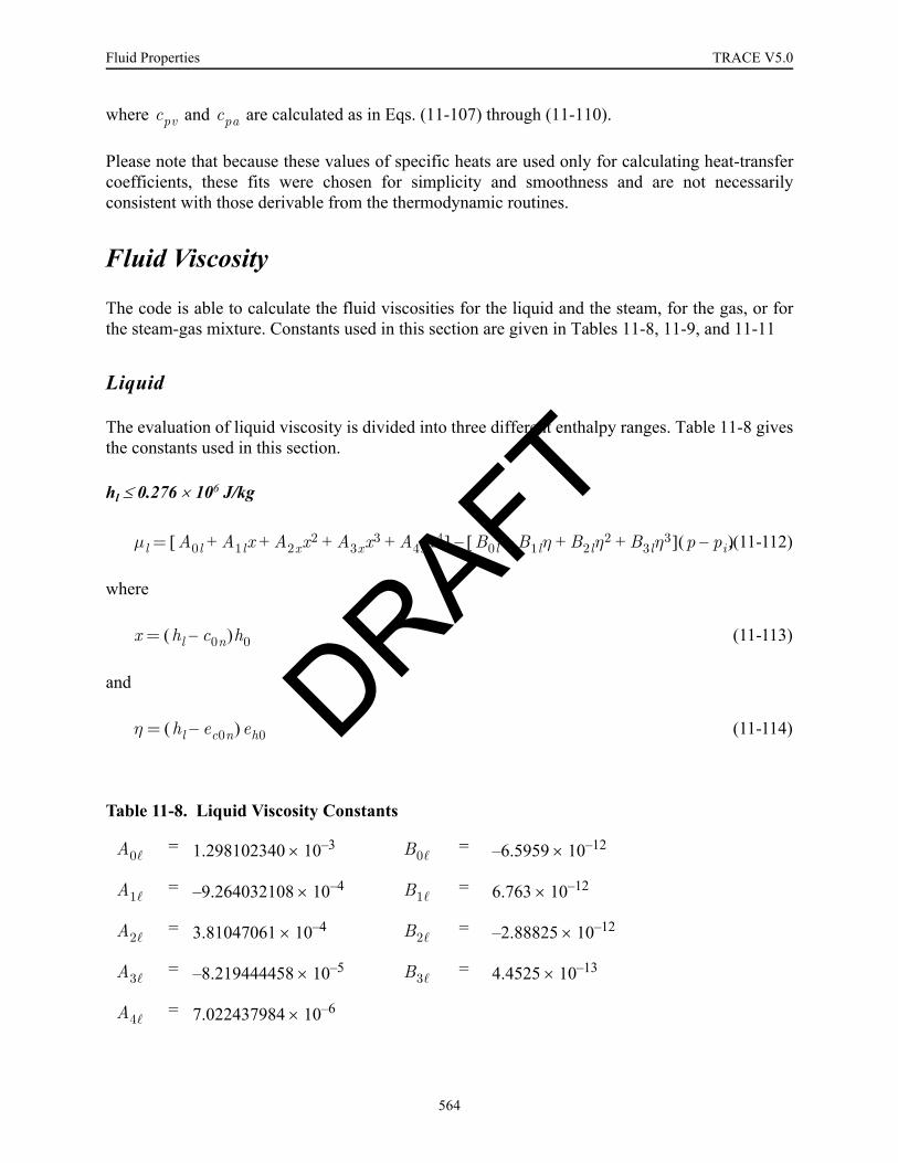
Fluid Properties TRACE V5.0
where and are calculated as in Eqs. (11-107) through (11-110).
Please note that because these values of specific heats are used only for calculating heat-transfercoefficients, these fits were chosen for simplicity and smoothness and are not necessarilyconsistent with those derivable from the thermodynamic routines.
Fluid Viscosity
The code is able to calculate the fluid viscosities for the liquid and the steam, for the gas, or forthe steam-gas mixture. Constants used in this section are given in Tables 11-8, 11-9, and 11-11
Liquid
The evaluation of liquid viscosity is divided into three different enthalpy ranges. Table 11-8 givesthe constants used in this section.
hl ≤ 0.276 × 10⁶ J/kg
,(11-112)
where
(11-113)
and
(11-114)
Table 11-8. Liquid Viscosity Constants
= 1.298102340 × 10–3 = –6.5959 × 10–12
= –9.264032108 × 10–4 = 6.763 × 10–12
= 3.81047061 × 10–4 = –2.88825 × 10–12
= –8.219444458 × 10–5 = 4.4525 × 10–13
= 7.022437984 × 10⁻⁶
cpv cpa
µl A0l A1lx A2xx2 A3xx3 A4xx4+ + + +[ ] B0l B1lη B2lη2 B3lη3+ + +[ ] p pi–( )–=
x hl c0n–( )h0=
η hl ec0n–( )eh0=
A0 B0
A1 B1
A2 B2
A3 B3
A4
DRAFT
564
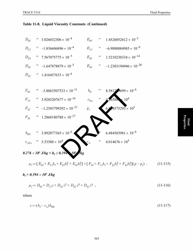
TRACE V5.0 Fluid Properties FOOBAR1234FOOBAR1234FOOBAR1234
Fluid Properties
0.276 × 10⁶ J/kg < hl ≤ 0.394 × 10⁶ J/kg
. (11-115)
hl > 0.394 × 10⁶ J/kg
, (11-116)
where
(11-117)
= 3.026032306 × 10–4 = 1.4526052612 × 10–3
= –1.836606896 × 10–4 = –6.9880084985 × 10–9
= 7.567075775 × 10–5 = 1.5210230334 × 10–14
= –1.647878879 × 10–5 = –1.2303194946 × 10–20
= 1.416457633 × 10–6
= –3.8063507533 × 10–11 = 8.581289699 × 10–6
= 3.9285207677 × 10–16 = 4.265884 × 104
= –1.2585799292 × 10–21 = 6.894575293 × 105
= 1.2860180788 × 10–27
= 3.892077365 × 10–6 = 6.484503981 × 10–6
= 5.53588 × 104 = 4.014676 × 10⁵
Table 11-8. Liquid Viscosity Constants (Continued)
D0 E0
D1 E1
D2 E2
D3 E3
D4
F0 h0
F1 c0n
F2 pi
F3
h00 eh0
ec0n cn
µl E0l E1lhl E2lhl2 E3lhl
3+ + +[ ] F0l F1lhl F2lhl2 F3lhl
3+ + +[ ] p pi–( )+=
µl D0l D1lz D2l z2 D3l z3 D4l z4+ + + +=
z hl cn–( )h00=
DRAFT
565
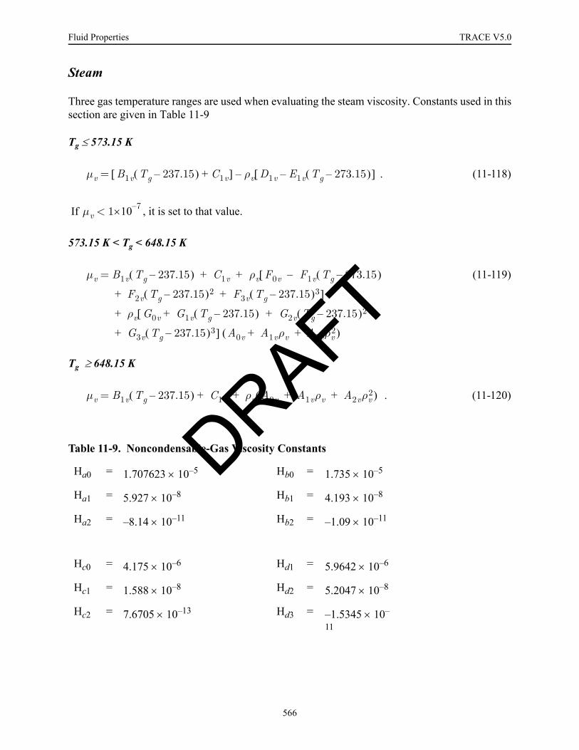
Fluid Properties TRACE V5.0
Steam
Three gas temperature ranges are used when evaluating the steam viscosity. Constants used in thissection are given in Table 11-9
Tg ≤ 573.15 K
. (11-118)
If , it is set to that value.
573.15 K < Tg < 648.15 K
(11-119)
Tg ≥ 648.15 K
. (11-120)
Table 11-9. Noncondensable-Gas Viscosity Constants
Ha0 = 1.707623 × 10⁻⁵ Hb0 = 1.735 × 10⁻⁵
Ha1 = 5.927 × 10⁻⁸ Hb1 = 4.193 × 10⁻⁸
Ha2 = –8.14 × 10⁻¹¹ Hb2 = –1.09 × 10⁻¹¹
Hc0 = 4.175 × 10⁻⁶ Hd1 = 5.9642 × 10⁻⁶
Hc1 = 1.588 × 10⁻⁸ Hd2 = 5.2047 × 10⁻⁸
Hc2 = 7.6705 × 10⁻¹³ Hd3 = –1.5345 × 10–
11
µv B1v Tg 237.15–( ) C1v+[ ] ρv D1v E1v Tg 273.15–( )–[ ]–=
µv 1 7–×10<
µv B1v Tg 237.15–( ) C1v ρv F0v F1v Tg 273.15–( )–
F2v Tg 237.15–( )2 F3v Tg 237.15–( )3+ +
[
]
ρv G0v G1v Tg 237.15–( ) G2v Tg 237.15–( )2
G3v Tg 237.15–( )3
+ +
+
[
] A0v A1vρv A2vρv2+ +( )
+ +
+
=
µv B1v Tg 237.15–( ) C1v ρv A0v A1vρv A2vρv2+ +( )+ +=
DRAFT
566

TRACE V5.0 Fluid Properties FOOBAR1234FOOBAR1234FOOBAR1234
Fluid Properties
Noncondensable Gas
The equations used for calculating the viscosity of noncondensible gases were obtained by fittinga quadratic polynomial to data with a least-squares method. The constants to these polynomialsare given in Table 11-10. The viscosity is not a strong functions of pressure (Ref. 11-16), so thecorrelations used for this quantity does not include a pressure dependence.
Air
If the noncondensable gas is air, two ranges of the gas temperature, , are used to determine thegas viscosity.
, (11-121)
where the polynomial constants and (for n=1 to 4) are given in Table 11-10.
The range of data over which the viscosity correlations for air was developed was273.15 K ≤ T ≤ 1073.15 K (Ref. 11-15). TRACE uses this correlation, however, for
Table 11-10. Noncondensable-Gas Viscosity Constants
Ha1 = 1.707623 × 10⁻⁵ N⋅ s⋅ m−2
Ha2 = 5.927 × 10⁻⁸ N⋅ s⋅(m2⋅ K)−1
Ha3 = −8.14 × 10⁻¹¹ N⋅ s⋅(m−2⋅ K−2)
Hb1 = 1.735 × 10⁻⁵ N⋅ s⋅ m−2
Hb2 = 4.193 × 10⁻⁸ N⋅ s⋅(m2⋅ K)−1
Hb3 = −1.09 × 10⁻¹¹ N⋅ s⋅(m−2⋅ K−2)
Hc1 = 4.175 × 10⁻⁶ N⋅ s⋅ m−2
Hc2 = 1.588 × 10⁻⁸ N⋅ s⋅(m2⋅ K)−1
Hc3 = 7.6705 × 10⁻¹³ N⋅ s⋅(m−2⋅ K−2)
Hd1 = 5.9642 × 10⁻⁶ N⋅ s⋅ m−2
Hd2 = 5.2047 × 10⁻⁸ N⋅ s⋅(m2⋅ K)−1
Hd3 = −1.5345 × 10⁻¹¹ N⋅ s⋅(m−2⋅ K−2)
Tg
µaHa1 Ha2 Tg 273.15–( ) Ha3 Tg 273.15–( )2+ + ; Tg 502.15 K≤
Hb1 Hb2 Tg 273.15–( ) Hb3 Tg 273.15–( )2+ + ; Tg 502.15 K>⎩⎪⎨⎪⎧
=
Han Hbn
DRAFT
567

Fluid Properties TRACE V5.0
273.15 K ≤ Tg ≤ 3000 K and 1.0 Pa ≤ P ≤ 45.0 MPa. The reference cited has no data for airviscosities with temperatures greater than 1073.15 K. However, Holman (Ref. 11-16) hasviscosity of air to 2773.15 K. Validation of the correlations against the Holman data within thecontext of TRAC-P and documented in its Theory Manual, show that as the temperature increasesfrom 1100 K to 2500 K, the percent error with respect to Holman grows approximately linearly,from less than 1% to 25% (underprediction). This is not generally considered to be a problem asTRACE will probably never have to calculate viscosity with such high temperatures, anyway.
Hydrogen
If the noncondensable gas is hydrogen, the gas viscosity is calculated as
, (11-122)
where the polynomial constants (for n=1 to 3) are given in Table 11-10.
As with the air correlations, the range of data over which the viscosity correlations for hydrogenwas developed was 273.15 K ≤ T ≤ 1073.15 K (Ref. 11-15). TRACE uses this correlation,however, for 273.15 K ≤ Tg ≤ 3000 K and 1.0 Pa ≤ P ≤ 45.0 MPa. The reference cited has no datafor hydrogen viscosities with temperatures greater than 1073.15 K. However, Holman (Ref. 11-16) has viscosity of hydrogen to 1173.15 K.
Helium
If the noncondensable gas is helium, the gas viscosity is calculated as
(11-123)
where the polynomial constants (for n=1 to 3) are given in Table 11-10.
The range of data over which the helium viscosity correlation was developed is255 K ≤ Tg ≤ 1090.15 K (Ref. 11-17). TRACE uses this correlation for 273.15 K ≤ Tg ≤ 3000 Kand 1.0 Pa ≤ P ≤ 45.0 MPa. The error associated with the viscosity of helium over the range273.15 K ≤ Tg ≤ 1090.15 K is no greater than 5.6%. The reference cited has no data for heliumviscosities at temperatures greater than 1090.15 K.
Steam-Gas Mixture
An averaging technique is used when calculating the viscosity of a steam-noncondensible gasmixture, such that
, (11-124)
µa Hc1 Hc2Tg Hc3Tg2+ +=
Hcn
µa Hd1 Hd2Tg Hd3Tg2+ +=
Hdn
µgp pa–( )µv paµa+
p--------------------------------------------=
DRAFT
568
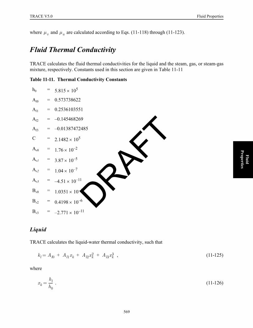
TRACE V5.0 Fluid Properties FOOBAR1234FOOBAR1234FOOBAR1234
Fluid Properties
where and are calculated according to Eqs. (11-118) through (11-123).
Fluid Thermal Conductivity
TRACE calculates the fluid thermal conductivities for the liquid and the steam, gas, or steam-gasmixture, respectively. Constants used in this section are given in Table 11-11
Liquid
TRACE calculates the liquid-water thermal conductivity, such that
, (11-125)
where
. (11-126)
Table 11-11. Thermal Conductivity Constants
h0 = 5.815 × 10⁵
Al0 = 0.573738622
Al1 = 0.2536103551
Al2 = –0.145468269
Al3 = –0.01387472485
C = 2.1482 × 10⁵
Av0 = 1.76 × 10⁻²
Av1 = 3.87 × 10⁻⁵
Av2 = 1.04 × 10⁻⁷
Av3 = –4.51 × 10⁻¹¹
Bv0 = 1.0351 × 10⁻⁴
Bv2 = 0.4198 × 10⁻⁶
Bv3 = –2.771 × 10⁻¹¹
µv µa
kl Al0 Al1xk Al2xk2 Al3xk
3+ + +=
xkhlh0-----=
DRAFT
569
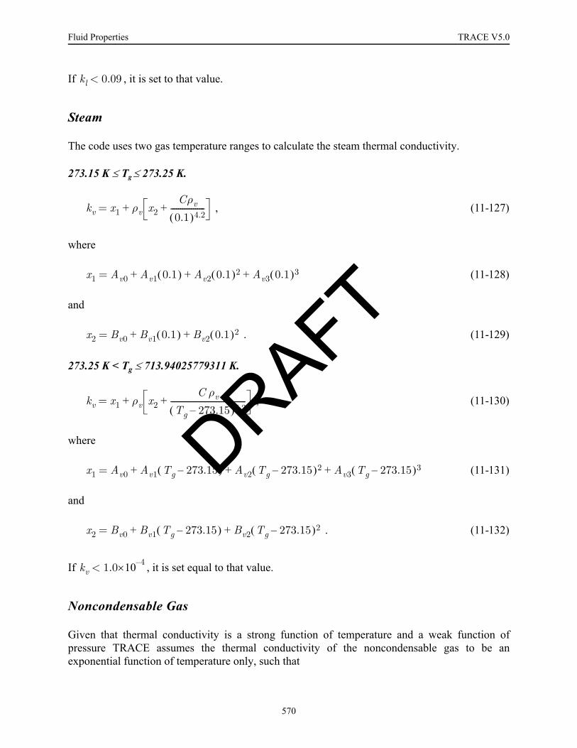
Fluid Properties TRACE V5.0
If , it is set to that value.
Steam
The code uses two gas temperature ranges to calculate the steam thermal conductivity.
273.15 K ≤ Tg ≤ 273.25 K.
, (11-127)
where
(11-128)
and
. (11-129)
273.25 K < Tg ≤ 713.94025779311 K.
, (11-130)
where
(11-131)
and
. (11-132)
If , it is set equal to that value.
Noncondensable Gas
Given that thermal conductivity is a strong function of temperature and a weak function ofpressure TRACE assumes the thermal conductivity of the noncondensable gas to be anexponential function of temperature only, such that
kl 0.09<
kv x1 ρv x2Cρv
0.1( )4.2------------------++=
x1 Av0 Av1 0.1( ) Av2 0.1( )2 Av3 0.1( )3+ + +=
x2 Bv0 Bv1 0.1( ) Bv2 0.1( )2+ +=
kv x1 ρv x2C ρv
Tg 273.15–( )4.2----------------------------------------++=
x1 Av0 Av1 Tg 273.15–( ) Av2 Tg 273.15–( )2 Av3 Tg 273.15–( )3+ + +=
x2 Bv0 Bv1 Tg 273.15–( ) Bv2 Tg 273.15–( )2+ +=
kv 1.0 4–×10<
DRAFT
570

TRACE V5.0 Fluid Properties FOOBAR1234FOOBAR1234FOOBAR1234
Fluid Properties
for air (11-133)
for hydrogen (11-134)
and
for helium (11-135)
This assumption should introduce inconsequential errors to most transients of interest in PWRs.
Steam-Gas Mixtures
TRACE uses an averaging technique to calculate the thermal conductivity of a steam-air, steam-hydrogen, or steam-helium mixture, such that
, (11-136)
where kv and ka are calculated as in Eqs. (11-127), (11-130) and (11-133) through (11-135).
Surface Tension
TRACE uses two ranges of the saturation temperature corresponding to the total pressure todetermine the surface tension of liquid water.
273.15 K ≤ Tsat ≤ 582.435 K.
Within this range, the surface tension of liquid water is calculated using the following ASMESteam Tables Recommended Interpolation Equation (Ref. 11-5):
. (11-137)
The ASME Steam Tables state that this equation is valid for temperatures between the triple point(273.16 K) and the critical point, which the reference assumes to be 647.15 K. It is necessary inTRACE, however, to place a lower limit on the calculated value of the surface tension to avoidsingularities when evaluating such things as the Chen nucleate-boiling relation. For this reason,the surface tension is set equal to a constant value for the remaining TRACE temperature range,582.435 K to 713.94025779311 K.
ka 2.091 4–×10 Tg0.846 [W/m K]·=
ka 1.6355 3–×10 Tg0.8213 [W/m K]·=
ka 3.366 3–×10 Tg0.668 [W/m K]·=
kgp pa–( )kv paka+
p------------------------------------------=
σ 0.2358 1 0.625647.15 Tsat–
647.15---------------------------------⎝ ⎠
⎛ ⎞–⎝ ⎠⎛ ⎞ 647.15 Tsat–
647.15---------------------------------⎝ ⎠
⎛ ⎞1.256
=
DRAFT
571

Fluid Properties TRACE V5.0
582.435 K < Tsat ≤ 713.94025779311 K
A constant value of surface tension is calculated in this range to keep the surface tension frombecoming too low. Constraining the temperature difference ratio to be no less than 0.1 gives
. (11-138)
Liquid Solute PropertiesTRACE has an extra mass-continuity equation for tracking a liquid solute (orthoboric acid or auser-defined solute) through all hydro components [see Eqs. (1-46) and (1-114) through (1-116)].If the liquid solute is orthoboric acid, its concentration in the reactor-core region can be used todetermine its neutronic reactivity-feedback effect on the point-reactor kinetics solution for thereactor-core power. The liquid solute has no other effect on the liquid-field processes andproperties. The equations solved in TRACE require a correlation for the maximum solubility ofthe solute material in liquid water.
Because there is no hydraulic feedback effect from the liquid solute on the fluid dynamic solution,the solute mass provides the capability to investigate numerical-diffusion effects and themovement and subsequent distribution of injected coolant.
Model Description
The solubility model for the solute is based on a simple linear correlation between the soluteconcentration and the liquid temperature. This model is appropriate for dilute solutions oforthoboric acid. The solubility model was developed based on information from Reference 11-19.
TRACE simulates orthoboric acid with its liquid solute model because of boron’s useful designcharacteristics. Boron has a thermal-neutron-capture cross section of 755 barns that can be used tointroduce negative neutronic reactivity to control the reactor-core power. Its referenceconcentration molality of 0.32 allows appropriate amounts to be dissolved in the liquid-watercoolant. Orthoboric acid is also physically and chemically very stable over its range of application(Ref. 11-20). The default solute in TRACE is orthoboric acid, which can be used in the reactivity-feedback calculation. If you wish to use a solute other than orthoboric acid, you can do so bydefining new solubility specifications through input (see the ISOLCN namelist variable).
TRACE calculates the solute concentration for both 1D and 3D components. The evaluationprocedure has two steps. The first step calculates the solute density and the second step calculatesthe amount of plated-out solute as well as the final solute concentration in each of thecomponent’s mesh cells for the time step.
σ 0.2358 1 0.625 0.1( )–[ ] 0.1( )1.256=
DRAFT
572

TRACE V5.0 Fluid Properties FOOBAR1234FOOBAR1234FOOBAR1234
Fluid Properties
TRACE calculates the solute density with Eq. (1-46). This equation calculates the solute densitydirectly, with no regard for the solubility of orthoboric acid or for the possible occurrence ofplating out. At this point, TRACE assumes infinite solubility of the material already in solution.In doing this calculation for any given mesh cell, the code considers each interface with anadjoining mesh cell. The amount of solute mass entering through a mesh-cell interface is definedby
(11-139)
where is the donor-cell liquid density, is the ratio of donor-cell solute mass to liquid mass,
and is the flow area between the mesh cells. The convected solute mass is evaluated implicitlyby its stabilizer mass equation.
The second set of calculations computes the amount of plated-out solute and obtains the finalliquid-solute-concentration ratio. If the cell has voided completely during the time step, all solutein the cell must have either convected out or plated out, and the liquid solute concentration is zero.If the cell has not voided completely (that is, if the cell still contains some liquid coolant),TRACE determines the maximum solubility of orthoboric acid as a function of temperature. Thissolubility value is known at 303 K and 373 K (Ref. 11-19). For temperatures between these twovalues, TRACE determines the solubility by linear interpolation. For temperatures less than303 K, TRACE uses the value at 303 K; for temperatures greater than 373 K, the code uses thevalue at 373 K. The maximum possible solute density is the water density times the maximumsolubility. If the new solute density exceeds this maximum, TRACE assumes the excess hasplated out, and the solute density becomes the maximum value. If the new solute density is lessthan the maximum, the code assumes that plated-out solute, if it exists in the cell, reenters solutionat an infinite rate to the extent that either all the plated-out solute dissolves or the solutionbecomes saturated. TRACE uses Eqs. (1-115) and (1-116) to calculate the final solute density andthe amount plated out. TRACE then finds the new concentration ratio by dividing the new solutedensity by the coolant density. Plated-out solute remains in the cell until it redissolves.
If a solute other than orthoboric acid is defined, you must input new maximum and minimumtemperatures, as well as solubility values for both temperatures. TRACE calculates the maximumsolubility using linear interpolation.
The boron concentration in orthoboric acid is one of four parameters that affect the neutronicreactivity of the reactor core. TRACE calculates their core-region averaged values in subroutineRFDBK. (For a more complete description of reactivity feedback, see Chapter 9). Whencalculating reactivity feedback from boron, TRACE takes into account all forms of boron in thereactor core,
1) dissolved orthoboric acid in the liquid coolant,
2) orthoboric acid plated on core structure,
3) borosilicate glass in burnable-poison pins, and
4) boron oxide in control-rod-cluster pins.
msolute Vl ρl m t∆ 1 α–( ) A· · · · ·=
ρl m
A
DRAFT
573
Fluid Properties TRACE V5.0
The solubility model for orthoboric acid affects items 1 and 2.
TRACE makes the following assumptions when implementing the solute-tracking feature of thecode:
1) The presence of solute in the coolant does not affect any of the liquid properties of the coolant, nor does it affect interfacial or wall heat transfer in any way (this assumption makes the solute concentration a good marker with which the fluid from a particular source can be followed).
2) While the code does allow for plated-out solute, it does not take into account the effects of such solute buildup except through neutronic reactivity feedback when the solute is orthoboric acid. Plated-out solute on structure surfaces could affect wall heat transfer and surface friction (Ref. 11-20).
3) Plating out occurs instantaneously if the concentration exceeds the maximum solubil-ity, such as when liquid coolant boils or flashes. Similarly, the plated-out material dis-solves at an infinite rate. No allowance is made for a supersaturated orthoboric solution.
4) The code assumes that the solubility is a function of temperature and is not pressure dependent.
5) The maximum-solubility temperature dependence is assumed to be linear and defined over a limited temperature range.
Reference 11-19 indicates that the maximum solubility of orthoboric acid at 303 K is 6.35 g/100 cm3 of water, and at 373 K, it is 27.6 g/100 cm3 of water. We interpreted this to meanrespective maximum solute concentrations of 0.0635 and 0.276 kg solute/kg water at 303 K and373 K; this interpretation is consistent with the data in Reference 11-21.
We are now aware of data that would permit the construction of a solubility curve in TRACE thatis valid over a much wider range of temperatures, although there is still a question of how to treatsolubility in the metastable range above 442 K. We believe that such a model should beincorporated. For now, the user can input a linearly-dependent maximum-solubility curve fit todata over the temperature range of interest if the default maximum-solubility curve isinappropriate. We do not believe that it is important to incorporate rates into the dissolution/plating processes because most transients in PWRs will not approach the solubility limits.
VerificationThe thermodynamic and transport property fits used in TRACE have been compared with steam-table data over a wide range of parameters. The agreement is satisfactory in the saturation region
and in the superheated steam region for p < and . For example, thesaturation temperature corresponding to a given pressure is always calculated within a maximum
pcritical Tg 823.0 K<
DRAFT
574

TRACE V5.0 Fluid Properties FOOBAR1234FOOBAR1234FOOBAR1234
Fluid Properties
error of ± 1 K. However, in most situations, the error is significantly smaller. The agreement also
is good in the subcooled-water region for .
Further verification was performed by comparing the TRACE polynomial fits with the WATERpackage (Ref. 11-1) over a wider range of nonequilibrium [99 K of both superheat and subcooling(liquid superheat or vapor subcooling exceeding 99 K are highly unlikely in reactor applications)]for pressures up to 20 MPa. The comparisons showed good agreement for both thethermodynamic and transport properties throughout the saturation and nonequilibrium regions,except for very extreme cases. However, at high degrees of subcooling or superheat, some minorinconsistencies were noticed. Because there are no data in these extreme cases, it is impossible tocompare TRACE and the WATER package adequately.
In addition, the output of the variables , , , and was checked against values generatedfrom the Sesame database. Sesame is a database, developed by members of the TheoreticalDivision at LANL, that includes various equation-of-state data (Ref. 11-6). For all of the resultsbelow, we used the EOSPAC program (Ref. 11-7) to read the Sesame data. Sesame material 7152(water) was used in these data comparisons. This particular data fit for water was originallydeveloped by the National Bureau of Standards [NBS, now known as the National Institute forStandards and Technology (NIST)]. A 64-term fit was used by the NBS to closely modelequation-of-state data (Ref. 11-8). Sesame data for material 7152 can be assumed to be accurateto within 1% for materials on the saturation line and within 5% for metastable regions off thesaturation line. Because the NBS data were based on a fit to experimental data for equilibriumstates, no attempt has been made to compare the data with our values for the metastable statescorresponding to subcooled steam or superheated liquid.
The values from the TRACE EOS package agreed very well with Sesame data. On the
saturation line at pressures below the critical pressure ( Pa,) the agreement
is excellent. Here the fractional error is less than 1%. Above (see Figure 11-1), the TRACE
values also agree with the Sesame data (dashed lines in graphs), often to better than 1%accuracy. However, there is a slight departure between the two curves in the pressure range
Pa. Here the fractional error is about 5%. For superheating, the plots near
the saturation line also appear good. For superheats of 8 K and less, the TRACE plot followsthe Sesame data fairly well. Larger than 10 K superheat yields fractional errors larger than 10%(Figure 11-2).
For the plot on the saturation line, Sesame and TRACE seem to agree well up to (Figure11-3). However, one significant departure is noted in the pressure range
Pa. Here, although the fractional error is only 0.5%, the slope of the
TRACE plot goes slightly negative in the pressure range Pa, while
Tl Tcritical<
pv ev e ρv
ρv
pcrit 2.2232 107×=
pcrit
ρv
pcrit pv 2.8 107×< <
ρv
ev pcrit
1.0 105× pv 2.0 106×< <
1.3 106× pv 2.0 106×< <
DRAFT
575

Fluid Properties TRACE V5.0
the Sesame slope remains positive. It should be noted that the TRACE slope is only slightlynegative, and then only for a short pressure range. At pressures above pcrit along the saturation line(Figure 11-3), the difference between the TRACE curve and the Sesame data becomes more
Figure. 11-1. Vapor density vs. pressure along the saturation line. Solid: TRACE; Dashed: Sesame.
Figure. 11-2. Vapor density vs. pressure at a superheat of 8 K. Solid: TRACE; Dashed: Sesame.
ev
DRAFT
576
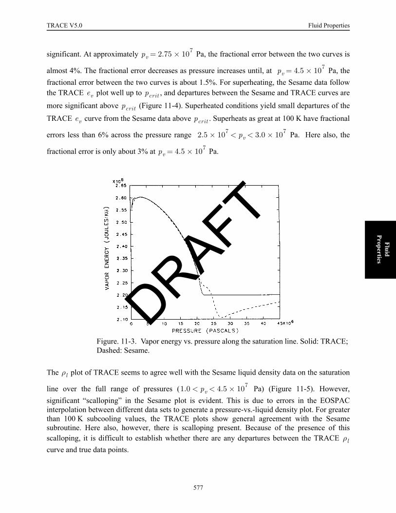
TRACE V5.0 Fluid Properties FOOBAR1234FOOBAR1234FOOBAR1234
Fluid Properties
significant. At approximately Pa, the fractional error between the two curves is
almost 4%. The fractional error decreases as pressure increases until, at Pa, thefractional error between the two curves is about 1.5%. For superheating, the Sesame data followthe TRACE plot well up to , and departures between the Sesame and TRACE curves are
more significant above (Figure 11-4). Superheated conditions yield small departures of the
TRACE curve from the Sesame data above . Superheats as great at 100 K have fractional
errors less than 6% across the pressure range Pa. Here also, the
fractional error is only about 3% at Pa.
The plot of TRACE seems to agree well with the Sesame liquid density data on the saturation
line over the full range of pressures ( Pa) (Figure 11-5). However,significant “scalloping” in the Sesame plot is evident. This is due to errors in the EOSPACinterpolation between different data sets to generate a pressure-vs.-liquid density plot. For greaterthan 100 K subcooling values, the TRACE plots show general agreement with the Sesamesubroutine. Here also, however, there is scalloping present. Because of the presence of thisscalloping, it is difficult to establish whether there are any departures between the TRACE curve and true data points.
Figure. 11-3. Vapor energy vs. pressure along the saturation line. Solid: TRACE; Dashed: Sesame.
pv 2.75 107×=
pv 4.5 107×=
ev pcrit
pcrit
ev pcrit
2.5 107× pv 3.0 107×< <
pv 4.5 107×=
ρl
1.0 pv 4.5 107×< <
ρl
DRAFT
577

Fluid Properties TRACE V5.0
Figure. 11-4. Vapor energy vs. pressure at a superheat of 8 K. Solid: TRACE; Dashed: Sesame.
Figure. 11-5. Liquid density vs. pressure along the saturation line. Solid: TRACE; Dashed: Sesame.
DRAFT
578

TRACE V5.0 Fluid Properties FOOBAR1234FOOBAR1234FOOBAR1234
Fluid Properties
The TRACE plot of on the saturation line agrees very well with the Sesame data for liquidinternal energy, at pressures below . In this range, accuracy appears to be far better than 1%.
At pressures above , a departure between the two curves is noted (Figure 11-6). In the
pressure range Pa, fractional errors as great as 8% between the
curves for the data are observed. These departures, however, occur when the curves of the
Sesame and TRACE plots are rising steeply. For this reason, the size of the fractional errors is
not as significant. Also, because the TRACE output variable must be input into the Sesameroutine to generate the Sesame data for liquid energy and because of the aforementioned difficultyin determining the accuracy of the TRACE data, it follows that the validity of departures in the
plots is also questionable. TRACE plots of subcooled liquid also follow Sesame data closely
(Figure 11-7). For subcooling as great as 100 K for pressures below , the TRACE and the
Sesame plots are quite close, with fractional errors in between the two curves of less than 1%.
The Sesame and TRACE curves, however, begin to depart in the region
Pa. Here the fractional errors in between the two curves reach as high as 8%, although theerrors are not as significant, as they again occur where both the Sesame and the TRACE curves
Figure. 11-6. Liquid energy vs. pressure along the saturation line. Solid: TRACE; Dashed: Sesame.
el
pcrit
pcrit
2.1 107× pv 3.0 107×< <
el
e
ρl
ρl
el el
pcrit
el
pcrit pv 3.3 107×< <
el
DRAFT
579

Fluid Properties TRACE V5.0
are rising steeply. At pressures above Pa, the curves begin to depart again, althoughhere reaching only a 3% fractional error.
In conclusion, for most TRACE applications, the thermodynamic and transport property routinesprovide realistic values up to the critical point.
Verification of Boron Solubility Model
TRACE will use the above model to calculate the solubility and concentration of orthoboric acidfor temperatures from 273.15 K, the triple-point temperature, to 647.3 K, the critical-pointtemperature of water. Figure 11-8 shows a comparison of the TRACE approximation forsolubility with the data from Reference 11-21; the data in Reference 11-20 are similar. The linearapproximation for the solubility of boric acid compares well with the data in the temperaturerange bounded by the two temperatures. On the low end of the temperature scale where weapproximate the solubility at 273 K by the solubility at 303, there is a 134% error. Reference 11-21 indicates that the solubility is 1 kg/kg water at 444 K, where there is a −72% error associatedwith the TRACE approximation. The solubility curve based on Reference 11-21 becomes verysteep as the temperature approaches 444 K.
If the solubility limits are exceeded, we believe that the typical result would be the creation of asupersaturated solution and/or a suspended precipitate that would not be plated out on thestructure surface.
Figure. 11-7. Liquid energy vs. pressure for 8 K subcooling. Solid: TRACE; Dashed: Sesame.
3.3 107×
DRAFT
580
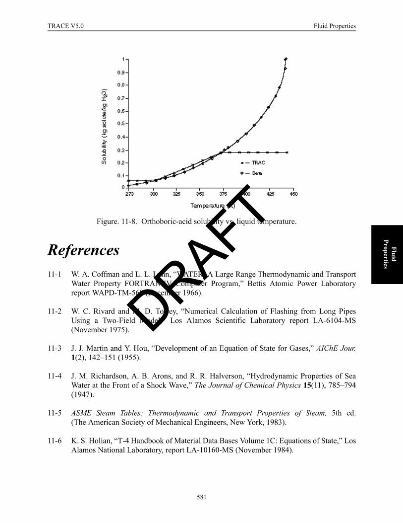
TRACE V5.0 Fluid Properties FOOBAR1234FOOBAR1234FOOBAR1234
Fluid Properties
References11-1 W. A. Coffman and L. L. Lynn, “WATER: A Large Range Thermodynamic and Transport
Water Property FORTRAN-IV Computer Program,” Bettis Atomic Power Laboratoryreport WAPD-TM-568 (December 1966).
11-2 W. C. Rivard and M. D. Torrey, “Numerical Calculation of Flashing from Long PipesUsing a Two-Field Model,” Los Alamos Scientific Laboratory report LA-6104-MS(November 1975).
11-3 J. J. Martin and Y. Hou, “Development of an Equation of State for Gases,” AIChE Jour.1(2), 142–151 (1955).
11-4 J. M. Richardson, A. B. Arons, and R. R. Halverson, “Hydrodynamic Properties of SeaWater at the Front of a Shock Wave,” The Journal of Chemical Physics 15(11), 785–794(1947).
11-5 ASME Steam Tables: Thermodynamic and Transport Properties of Steam, 5th ed.(The American Society of Mechanical Engineers, New York, 1983).
11-6 K. S. Holian, “T-4 Handbook of Material Data Bases Volume 1C: Equations of State,” LosAlamos National Laboratory, report LA-10160-MS (November 1984).
Figure. 11-8. Orthoboric-acid solubility vs. liquid temperature.
DRAFT
581

Fluid Properties TRACE V5.0
11-7 C. Cranfill, “EOSPAC: A Subroutine Package for Accessing the Los Alamos Sesame EOSData Library,” Los Alamos National Laboratory report LA-9728-M (August 1983).
11-8 L. Haar, J. Gallagher, and G. Kell, “A Thermodynamic Surface for Water:The Formulation and Computer Program,” National Bureau of Standards reportNBSIR 81-2253 (May 1981).
11-9 K. Watanabe, R.B. Dooley, IAPWS Release on the IAPWS Formulation 1995 for theThermodynamic Properties of Ordinary Water Substance for General and Scientific Use,Fredericia, Denmark, Sept. 1996.
11-10 J. W. Spore, Pratap Sadasivan, D. R. Liles,‘‘Accelerator Transmutation of Waste Updatesfor TRAC-M’’, LA-UR-01-3660, June 2001.
11-11 Jay W. Spore, D.R. Liles, ‘‘Improvements to the Accelerator Transmutation of WasteUpdates for TRAC-M’’, LA-UR-01-6219, September 2001.
11-12 The Thermal Hydraulics Group, RELAP5/MOD3 CODE MANUAL, VOLUME I: CODESTRUCTURE, SYSTEM MODELS,AND SOLUTION METHODS, NUREG/CR-5535-Vol. I, June 1999.
11-13 The Thermal Hydraulics Group, RELAP5/MOD3 CODE MANUAL, VOLUME IV:MODELS AND CORRELATIONS, NUREG/CR-5535 Volume IV, June 1999.
11-14 Frank M. White, Fluid Mechanics (McGraw-Hill Book Co., Inc., New York, 1979).
11-15 Kuzman Raznjevic, Handbook of Thermodynamic Tables and Charts (McGraw-Hill BookCo., Inc., New York, 1976).
11-16 J. P. Holman, Heat Transfer (McGraw-Hill Book Co., Inc., New York, 1981).
11-17 J. M. Sicilian and R. P. Harper, Heavy-Water Properties for the Transient Reactor AnalysisCode, Flow Science, Inc. report FSI-85-Q6-1 (1985).
11-18 E. A. Haytcher and J. C. Lin, “Modification to Helium Properties in the TRAC-PF1/MOD2 Code,” Los Alamos National Laboratory report LA-N7-1 (December 1992).
11-19 CRC Handbook of Chemistry and Physics, 62nd ed., p. B-84, (The CRC Press, Inc., BocaRaton, Florida, 1981).
11-20 Paul Cohen, Water Coolant Technology of Power Reactors, pp. 218-221, (Gordon andBreach Science Publishers, New York, 1969).
11-21 Leopold Gmelin, Gmelins Handbuch der Anorganischen Chemie, Supplement toVolume 1, System Number 13 (Boron), pp. 149-156, (Verlag Chemie, Gmbh., Weinheim/Bergstrasse, 1954).
DRAFT
582

TRACE V5.0 Structural Material Properties FOOBAR1234FOOBAR1234FOOBAR1234FOOBAR1234
Structural M
aterial Properties
12 Structural Material PropertiesFOOBAR1234FOOBAR1234FOOBAR1234FOOBAR1234FOOBAR1234
An extensive library of temperature-dependent material properties is incorporated in the TRACEcode. The entire library is accessible by the HTSTR (heat-structure) component while theremaining components have access to structural material-property sets only. There are 12 sets ofmaterial properties that make up the library. Each set supplies values for thermal conductivity,specific heat, density, and spectral emissivity for use in the heat-transfer calculations.
The material indexes in the library are
1 – mixed-oxide fuel;2 – Zircaloy;3 – fuel-clad gap gases;4 – boron-nitride insulation;5 – Constantan/Nichrome heater coil;6 – stainless steel, type 304;7 – stainless steel, type 316;8 – stainless steel, type 347;9 – carbon steel, type A508;
10 – Inconel, type 718;11 – Zircaloy dioxide; and12 – Inconel, type 600.
The first three sets and set 11 contain properties for materials that are part of nuclear fuel rods.Properties for these materials, including models for thermal expansion that are important as rodsdeform, are discussed in Chapter 8. Sets 4 and 5 are used in modeling electrically heated fuelrod simulators, which are used in many separate and integral test facilities. Sets 6 through 10 andset 12 are for structural materials, including stainless steels, carbon steel, and Inconels. Propertiesfor sets 4 through 10 and 12 are discussed in this section. In addition, since other materialproperties may be necessary to model a test facility or plant, TRACE includes an option thatenables you to define and supply properties for materials not included in the above list.
NomenclatureThe following nomenclature is used in this section:
DRAFT
583

Structural Material Properties TRACE V5.0
= specific heat capacity at constant pressure (J · kg–1 · K–1)
= thermal conductivity (W/m/K)
= pressure (Pa)
= temperature (K)
= temperature (°C)
= temperature (°F)
= emissivity
= density (kg/m3)
Electrical Fuel-Rod Insulator (BN) PropertiesThe code calculates values for boron nitride insulators that are used in electrically heated nuclearfuel-rod simulators. Magnesium oxide insulators are assumed to have roughly equivalent values.
Density
A constant value of 2002.0 kg/m3 from Reference 12-1 is used.
Specific Heat
A four-term polynomial is used to calculate the specific heat. The independent variable istemperature in degrees Fahrenheit, and the constants, which are modifications of those reported inan EPRI report (Ref. 12-2), are listed in the equation below:
(12-1)
Thermal Conductivity
The boron-nitride thermal-conductivity calculation, based on a conversion to SI units of a curvefit reported in Reference 12-3, is
. (12-2)
cp
k
p
T
TC
TF
ε
ρ
cp 760.59 1.7955TF 8.6704 4–×10 TF2– 1.5896 7–×10 TF
3+ +=
k 25.27 1.365 10 3– TF×–=
DRAFT
584

TRACE V5.0 Structural Material Properties FOOBAR1234FOOBAR1234FOOBAR1234FOOBAR1234
Structural M
aterial Properties
Spectral Emissivity
A constant value of unity is used for the boron nitride spectral emissivity.
Electrical Fuel-Rod Heater-Coil (Constantan) PropertiesThe code calculates property values for Constantan heater coils as used in electrically heatednuclear fuel-rod simulators. We assume that Nichrome coils, used in some installations in place ofConstantan, have similar properties. The correlations used are from Reference 12-3.
Density
A constant value of 8393.4 kg/m3 is used.
Specific Heat
The specific heat is
(12-3)
Thermal Conductivity
The thermal conductivity is given by
. (12-4)
Spectral Emissivity
A constant value of unity is used.
Structural Material PropertiesThe code supplies property values for six types of structural materials normally used in LWRs:stainless steel, type 304; stainless steel, type 316; stainless steel, type 347; carbon steel, type
cp 110TF0.2075=
k 29.18 2.683 10 3– TF 100–( )×+=
DRAFT
585

Structural Material Properties TRACE V5.0
A508; and Inconel, types 718 and 600. These properties were obtained from Reference 12-3through Reference 12-6. A tabulation of the correlations used is given in Tables 12-1 through12-6.
Table 12-1. Stainless Steel, Type 304, Properties
PropertyIndependent
Variable Polynomial ConstantsReference Number
ρ T a0 = 7984.0 12-4
a1 = –2.651 × 10–
a2 = –1.158 × 10⁻⁴
cp a0 = 426.17 12-4
a1 = 0.43816
a2 = –6.3759 × 10⁻⁴
a3 = 4.4803 × 10⁻⁷
a4 = –1.0729 × 10⁻¹⁰
k T a0 = 8.116 12-4
a1 = 1.618 × 10⁻²
ε — a0 = 0.84 12-4
ρ = density (kg ⋅ m–3)cp = specific heat (J ⋅ kg–1 ⋅ K–1)k = thermal conductivity (W ⋅ m–1 ⋅ K–1)T = temperature (K)
= temperature (°F)y = a0 + a1x + a2x2 + … + amxm
Table 12-2. Stainless Steel, Type 316, Properties
PropertyIndependent
Variable Polynomial ConstantsReference Number
ρ T a0 = 8084.0 12-5
a1 = –4.209 × 10⁻¹
a2 = –3.894 × 10⁻⁵
TF
TF
DRAFT
586

TRACE V5.0 Structural Material Properties FOOBAR1234FOOBAR1234FOOBAR1234FOOBAR1234
Structural M
aterial Properties
cp a0 = 426.17 12-5
a1 = 0.43816
a2 = -6.3759 × 10⁻⁴
a3 = 4.4803 × 10⁻⁷
a4 = -1.7029 × 10⁻¹⁰
k T a0 = 9.248 12-5
a1 = 1.571 × 10⁻²
ε — a0 = 0.84 12-5
ρ = density (kg ⋅ m–3)cp = specific heat (J ⋅ kg–1 ⋅ K–1)k = thermal conductivity (W ⋅ m–1 ⋅ K–1)T = temperature (K)
= temperature (°F)y = a0 + a1x + a2x2 + … + amxm
Table 12-3. Stainless Steel, Type 347, Properties
PropertyIndependent
Variable Polynomial ConstantsReference Number
ρ T a0 = 7913.0 12-3
cp ( – 240) a0 = 502.416 12-3
a1 = 0.0984
k a0 = 14.1926 12-3
a1 = 7.269 × 10⁻³
ε — a0 = 0.84 12-3
Table 12-2. Stainless Steel, Type 316, Properties
PropertyIndependent
Variable Polynomial ConstantsReference Number
TF
TF
TF
TF
DRAFT
587
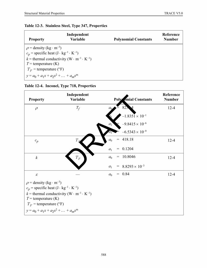
Structural Material Properties TRACE V5.0
ρ = density (kg ⋅ m–3)cp = specific heat (J ⋅ kg–1 ⋅ K–1)k = thermal conductivity (W ⋅ m–1 ⋅ K–1)T = temperature (K)
= temperature (°F)y = a0 + a1x + a2x2 + … + amxm
Table 12-4. Inconel, Type 718, Properties
PropertyIndependent
Variable Polynomial ConstantsReference Number
ρ Tf a0 = 8233.4 12-4
a1 = –1.8351 × 10⁻¹
a2 = –9.8415 × 10⁻⁶
a3 = –6.5343 × 10⁻⁹
cp a0 = 418.18 12-4
a1 = 0.1204
k a0 = 10.8046 12-4
a1 = 8.8293 × 10⁻³
ε — a0 = 0.84 12-4
ρ = density (kg ⋅ m–3)cp = specific heat (J ⋅ kg–1 ⋅ K–1)k = thermal conductivity (W ⋅ m–1 ⋅ K–1)T = temperature (K)
= temperature (°F)y = a0 + a1x + a2x2 + … + amxm
Table 12-3. Stainless Steel, Type 347, Properties
PropertyIndependent
Variable Polynomial ConstantsReference Number
TF
TF
TF
TF
DRAFT
588
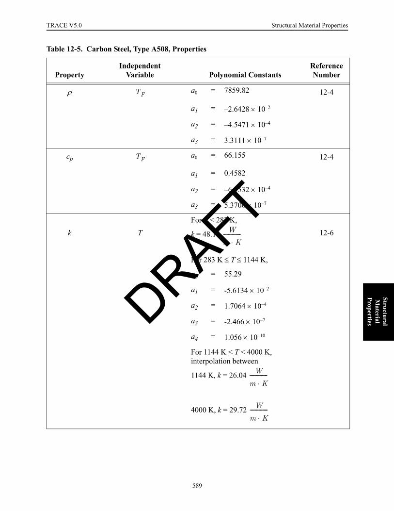
TRACE V5.0 Structural Material Properties FOOBAR1234FOOBAR1234FOOBAR1234FOOBAR1234
Structural M
aterial Properties
Table 12-5. Carbon Steel, Type A508, Properties
PropertyIndependent
Variable Polynomial ConstantsReference Number
ρ a0 = 7859.82 12-4
a1 = –2.6428 × 10⁻²
a2 = –4.5471 × 10⁻⁴
a3 = 3.3111 × 10⁻⁷
cp a0 = 66.155 12-4
a1 = 0.4582
a2 = –6.5532 × 10⁻⁴
a3 = 5.3706 × 10⁻⁷
k T
For T < 283 K,
k = 48.16 12-6
For 283 K ≤ T ≤ 1144 K,
a0 = 55.29
a1 = -5.6134 × 10⁻²
a2 = 1.7064 × 10⁻⁴
a3 = -2.466 × 10⁻⁷
a4 = 1.056 × 10⁻¹⁰
For 1144 K < T < 4000 K,interpolation between
1144 K, k = 26.04
4000 K, k = 29.72
TF
TF
W
m K·--------------
W
m K·--------------
W
m K·--------------
DRAFT
589
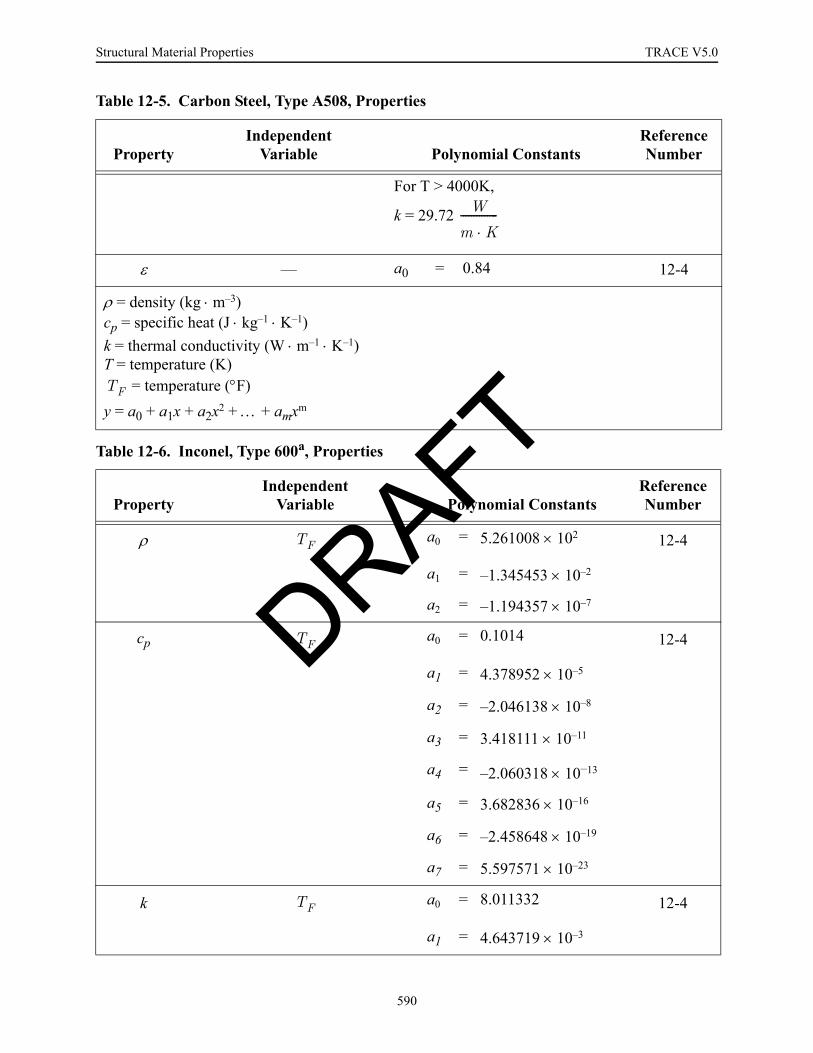
Structural Material Properties TRACE V5.0
For T > 4000K,
k = 29.72
ε — a0 = 0.84 12-4
ρ = density (kg ⋅ m–3)cp = specific heat (J ⋅ kg–1 ⋅ K–1)k = thermal conductivity (W ⋅ m–1 ⋅ K–1)T = temperature (K)
= temperature (°F)y = a0 + a1x + a2x2 + … + amxm
Table 12-6. Inconel, Type 600a, Properties
PropertyIndependent
Variable Polynomial ConstantsReference Number
ρ a0 = 5.261008 × 10² 12-4
a1 = –1.345453 × 10⁻²
a2 = –1.194357 × 10⁻⁷
cp a0 = 0.1014 12-4
a1 = 4.378952 × 10⁻⁵
a2 = –2.046138 × 10⁻⁸
a3 = 3.418111 × 10⁻¹¹
a4 = –2.060318 × 10⁻¹³
a5 = 3.682836 × 10⁻¹⁶
a6 = –2.458648 × 10⁻¹⁹
a7 = 5.597571 × 10⁻²³
k a0 = 8.011332 12-4
a1 = 4.643719 × 10⁻³
Table 12-5. Carbon Steel, Type A508, Properties
PropertyIndependent
Variable Polynomial ConstantsReference Number
W
m K·--------------
TF
TF
TF
TF
DRAFT
590

TRACE V5.0 Structural Material Properties FOOBAR1234FOOBAR1234FOOBAR1234FOOBAR1234
Structural M
aterial Properties
References12-1 Y. S. Touloukian, editor, Thermophysical Properties of High Temperature Solid Materials
(MacMillan Co., New York, 1967).
12-2 “A Prediction of the SEMISCALE Blowdown Heat Transfer Test S-02-8 (NRC StandardProblem Five),” Electric Power Research Institute report EPRI/NP-212 (October 1976).
12-3 W. L. Kirchner, “Reflood Heat Transfer in a Light Water Reactor,” US Nuclear RegulatoryCommission report (NUREG-0106) Vols. I and II (August 1976).
12-4 J. C. Spanner, editor, “Nuclear Systems Materials Handbook—Vol. 1 Design Data,”Hanford Engineering Development Laboratory report TID-26666 (1976).
12-5 “Properties for LMFBR Safety Analysis,” Argonne National Laboratory reportANL-CEN-RSD-76-1 (1976).
a2 = 1.872857 × 10⁻⁶
a3 = –3.914512 × 10⁻⁹
a4 = 3.475513 × 10⁻¹²
a5 = –9.936 696 × 10–16
ε — a0 = 0.84 12-4
ρ = density (kg ⋅ m–3)cp = specific heat (J ⋅ kg–1 ⋅ K–1)k = thermal conductivity (W ⋅ m–1 ⋅ K–1)T = temperature (K)
= temperature (°F)y = a0 + a1x + a2x2 + … + amxm
a. Inconel type 600 coefficients are in British units; ρ is multiplied by 16.01846 (kg·m–3)/(lbm·ft–3), cp by
4.1868 × 10³ (J·kg–1·K)/(Btu·lbm–1·°F–1), and k by 1.729577 (W·m–1·K–1)/(Btu·h–1·ft–1·°F–1). The
conversion factor for the thermal conductivity k assumes the thermochemical BTU instead of theinternational BTU.
Table 12-6. Inconel, Type 600a, Properties
PropertyIndependent
Variable Polynomial ConstantsReference Number
TF
DRAFT
591

Structural Material Properties TRACE V5.0
12-6 ASME Boiler and Pressure Vessel Code, Section II, Part D - Properties, American Societyof Mechanical Engineers, 2001
DRAFT
592

TRACE V5.0 Quasi-Steady Assumption and Averaging Operators FOOBAR1234FOOBAR1234FOOBAR1234FOOBAR1234FOOBAR1234
Quasi-Steady
Assum
ption and A
veraging
A Quasi-Steady Assumption and
Averaging OperatorsFOOBAR1234FOOBAR1234FOOBAR1234FOOBAR1234FOOBAR1234FOOBAR1234
The coupled-equation set that combines the single-phase, multidimensional, fluid field equationsfor mass, momentum, and energy with the equation for heat diffusion within a bounding wall iscalled the conjugate problem. The transient two-phase flow problem becomes even more difficultbecause an additional set of field equations for the second fluid phase must be solvedsimultaneously together with the necessary closure relations to couple the two fluid phases. TheTRACE code, as well as most other similar codes, invokes a quasi-steady approach to the heat-transfer coupling between the wall and the fluid as well as the closure relations for interfacial heattransfer and drag and wall-to-fluid drag. This quasi-steady approach assumes detailed knowledgeof the local fluid parameters and ignores time dependencies such that the time rate of change inthe closure relationships becomes infinite and the time constants are zero. The quasi-steadyapproach has the advantages of being reasonably simple and generally applicable to a wide rangeof problems and of not requiring previous knowledge of the given transient.
In this appendix, the quasi-steady approach and the averaging operators used in TRACE arediscussed.
Nomenclature = area
= fraction of wall contacted by gas
= fraction of wall contacted by liquid
= area fraction contacted by liquid
= local phasic heat flux
= total heat flux
= area-averaged effective phasic heat flux
A
Awg
Awl
fl
q
qtotal
q′
DRAFT
593

Quasi-Steady Assumption and Averaging Operators TRACE V5.0
= area-averaged phasic heat fluxS = dimensionless number defined by Eq. (A-20)
= time
= generic for independent variable
= generic for dependent variable
Greek or = time-step size
= ratio of transient and phenomenological time constants
= transient time constraint
= phenomenological time constant
= weighting factor between old- and new-time values
Subscripts = gas
= independent-variable indices
= liquid
= maximum
= minimum
= quasi-steady
= steady state
= transient
= old-time weighted new-time value
= wall
= wall-to-gas
= wall to-liquid
Superscripts = new-time value
= old-time value
q″
t
X
Y
t∆ δt
θ
τ
τc
ψ
g
i
l
max
min
qs
ss
tr
used
w
wg
wl
n
n 1–
DRAFT
594

TRACE V5.0 Quasi-Steady Assumption and Averaging Operators FOOBAR1234FOOBAR1234FOOBAR1234FOOBAR1234FOOBAR1234
Quasi-Steady
Assum
ption and A
veraging
IntroductionAn alternative to the quasi-steady approach does exist on a case-by-case basis. If the necessaryinitial and boundary conditions are known, the solution of the conjugate problem requires a prioriknowledge of the wall-to-fluid convective heat transfer. Studies such as those of Sucec (Refs. A-7and A-8) have used this latter approach to obtain both analytical and numerical solutions for manysingle-phase transients. The results, when compared to those using the quasi-steady approach,have led to an understanding of the conditions under which the quasi-steady approach producesvalid results.
For the heat-transfer coupling between the wall and the fluid, the quasi-steady approach workswell provided that the fluid responds more rapidly than the wall. For example, the fluid boundarylayer responds so quickly that the surface temperature of a thick, high-conductivity wall does nothave time to change. When the wall changes faster than the fluid, however, one must use transientclosure relations to solve the problem accurately.
Despite the difficulties and limitations of the quasi-steady solution approach to the conjugateproblem for two-phase flow, this approach is the only method available to simulate transientconditions in large, complex, two-phase systems such as a nuclear power plant. Often, in order toobtain an answer to a difficult problem, engineers apply codes like TRACE even when the quasi-steady assumption is not valid. The literature does contain many papers in which the closurerelationships have been modified to obtain agreement with what is, in fact, transient data.Although this process can provide valuable insight, the resulting relationships may be misleadingand may produce inaccurate results when applied either to other transient experiments or to trulyquasi-steady transients. Unfortunately, within the English literature, there are very few systematicstudies of the problems inherent to the quasi-steady assumptions. The initial study by Nelson(Ref. A-9) and the more recent work of Pasamehmetoglu and Nelson (Ref. A-10) do address theproblem. As Kuznetsov (Ref. A-11) presented in his overview, the Soviets at least may havedefined more clearly the existence of these limitations.
Chapter 1 indicated the importance of the quasi-steady assumption and the averaging operators(volume and temporal) on the closure relationships. While these considerations are of equalimportance to all the closure relationships, it is not possible to discuss each set individually. Thissection will investigate those considerations relative to the wall-to-fluid heat-transfer process.Extension to the other relationships follows similar logic.
The wall-to-fluid heat transfer appears in the two-phase-fluid equation set within the total-energyequation as and the combined-gas-energy equation as . These terms, and ,represent the rate of sensible energy per unit volume being transferred into the phasic componentsof the fluid [see Chapter 1, Eqs. (1-28) and (1-29)]. Mass transfer resulting from the superheatingof a liquid and its subsequent evaporation, for example, must take place through the phasic-change equation represented by Eqs. (1-25) through (1-27) in Chapter 1. The total wall-to-fluidheat flux, is also required in order to provide the boundary condition necessary for thesolution of all structures exposed to the fluid.
qwl qwg+ qwg qwl qwg
q′wl q′wg+
DRAFT
595

Quasi-Steady Assumption and Averaging Operators TRACE V5.0
Perhaps the easiest way to envision these phasic terms arising is to realize that, within the volume-averaged equations, the total surface area over which one integrates can be decomposed into twoparts [see term number 5 of Reference A-12, Eq. (2-125), p. 70]. One part has liquid contacting itwhile the other has gas contacting it, so that
. (A-5)
Thus,
. (A-6)
By defining the following terms,
, (A-7)
, (A-8)
and
, (A-9)
Eq. (A-6) becomes
, (A-10)
where
.
Integration of Eqs. (A-6) through (A-10) with respect to time is an obvious step not shown hereand produces “volume-time” averaged quantities required by the two-phase conservationequations [see Chapter 1, Eqs. (1-11) through (1-16)]. The time interval over which the
Aw Awl Awg+=
q AdAw
∫ q AdAwt
∫ q AdAwg
∫+=
q AdAwl
∫ qwl″ Awl≡
q AdAwg
∫ qwg″ Awg≡
q AdAw
∫ qtotal Aw≡
qtotal q′wg q′wl+ q″wl fl q″wg 1 fl–( )+= =
flAwlAw---------=
δt
DRAFT
596
TRACE V5.0 Quasi-Steady Assumption and Averaging Operators FOOBAR1234FOOBAR1234FOOBAR1234FOOBAR1234FOOBAR1234
Quasi-Steady
Assum
ption and A
veraging
integration is performed must meet those requirements described by Bergles et al. (Ref. A-12).The right-hand sides of Eqs. (A-7) through (A-9) and Eq. (A-10) are assumed to reflect thetemporal averaging without any further notation change.
The influence of the spatial-averaging operator is realized principally through its influence in datareduction and is therefore inherent within the closure relationships. The code makes no checks toinvestigate the influence of the spatial averaging; we discuss this in greater detail below in thesection Spatial-Averaging Operator.
A temporal effect is present in both the quasi-steady assumption and the temporal-averagingoperator. To further differentiate between the problems that may arise from these two sources, wewill first assume that the transient under consideration is slow enough that the quasi-steadyassumption is valid. The question becomes what is the relationship among the time-step sizedesired by the code, , the time constant of the physical phenomena, (the minimum time of
integration for the temporal averager), and the time constant of the transient, (some fraction ofthis time will be the maximum time of integration for the temporal averager). This relationship isthe point raised by Bergles, et al. (Ref. A-12), which was noted earlier. Nelson (Ref. A-9) furtherrefined the question concerning the minimum time of integration, denoted as , by pointing
out that must include a sufficient number of events of the governing phenomena, reflected
by , to make the integral “independent” of time. Therefore, the question becomes what should
happen when .
Generally, the second part of the above question, is not important in TRACE becausecalculations are controlled frequently by the rate of change of the quantities. In the future,however, as time-step sizes continue to increase as a result of improved numerics, this portion ofthe question may become more important. For TRACE, the first part of the question is importantand is a condition that frequently arises in the code. Again, Nelson (Ref. A-9) has pointed out thatin addressing this question, we must decide which of two questions we wish to answer. If we wishto model the instantaneous response inside the time interval represented by , a transientclosure model is required even for “steady-state” conditions. In general, this representation isbeyond the state of the art. Thus, only the average response during these “small” time steps,
, can be defined and the quasi-steady closure relationship should be constant over the
time interval corresponding to . Early in the TRACE development, we observed the effect
of and developed crude averagers to minimize the observed problems. (It is not clear thatearly code developers had interpreted these problems as arising from this cause.) Only recentlyhave calculations again identified these temporal-averaging problems as significant; the newobservations center on noding and time-step sensitivities in the calculated results. The sectionsAveragers and Limiters Arising from Temporal-Averager Considerations and Variations in the
t∆ τc
τ
δtmin
δtmin
τc
∆t δtminor∆t τ><
∆t τ>
δtmin
∆t δtmin<
δtmin
δtmin
DRAFT
597

Quasi-Steady Assumption and Averaging Operators TRACE V5.0
Application of Temporal Averagers and Limiters will discuss the models currently in TRACE to
address this problem of .
In the preceding discussion, we assumed the quasi-steady assumption was valid. The questionremains as to when the assumption breaks down. As pointed out by Nelson (Ref. A-9), one way ofperceiving this breakdown arises from temporal-averaging considerations. The observedcharacteristic is that when is decreased to the , the resulting quantity will still show a
sensitivity to . Once this happens, the transient is a true transient. The section Validity of theQuasi-Steady Assumption will discuss more recent techniques for determining when the quasi-steady assumption is valid. Because the code at this time only implements the quasi-steadyassumption, we offer no alternative procedures for dealing with a true transient.
Averagers and Limiters Arising from Temporal-Averager ConsiderationsA potential problem that one sees in transient analysis using the quasi-steady approach is that theclosure relations are free to respond instantaneously (within a single time step) to any changesoccurring within the flow field. Thus, unless some type of averager and/or limiter is used, flowregimes may change instantly. While the averagers/limiters used in TRACE vary among closurepackages, they are typically represented by the following relations. Averagers from one time stepto the next generally appear as
, (A-11)
where represents some closure quantity, is a fraction between zero and one, and the
superscripts and indicate old- and new-time values of , respectively. The is the
closure-relationship value used in the current time step and becomes for the next time step.Thus, as approaches one, would change very slowly, and for equal to zero, would change instantly. Typical limiters are given as
,
where and are reasonable bounds for and depend on the phenomenon addressedby the closure relationship.
A third approach is to use an averager equation that is based on the time step size and the timeconstant for the phenomena of interest. For example, Eq. (A-12) is an averager formula that is
∆t δtmin<
t∆ δtmin
t∆
Ynused ψYn 1– 1 ψ–( )Yn+=
Y ψ
n 1– n Y Ynused
Yn 1–
ψ Yused ψ Yused
Ymin Yn Ymax< <
Ymin Ymax Y
DRAFT
598

TRACE V5.0 Quasi-Steady Assumption and Averaging Operators FOOBAR1234FOOBAR1234FOOBAR1234FOOBAR1234FOOBAR1234
Quasi-Steady
Assum
ption and A
veraging
relatively simple to evaluate and has consistent limits as the time step size decrease to smallvalues or increases to large values.
(A-12)
In the limit as the time step size approaches zero, approaches and as the time step
size becomes large relative to the time constant for the phenomena of interest, approaches
. When the time step size is the same order of magnitude as the time constant for the
phenomena of interest, then is an average of old and new predicted parameter. The timeaverager formula given by Eq. (A-12) eliminates some of the time step sensitivities that appearwhen Eq. (A-11) is used.
An alternative method to these averagers and/or limiters is the use of additional transportequations within the code to convect such quantities as interfacial area or drop/bubble diameter.While these transport equations do “stabilize” the potential “instantaneous-response” problem,however, they do not directly address the problem that still exists—that the closure relationshipsare quasi-steady at best.
Variations in the Application of Temporal Averagers and LimitersThe problem with the above averager [given by Eq. (A-11)] is that it produces a time-averagingscheme which is time-step-size dependent. For example, if we were to run a transient calculationwith a fixed time-step size of 100 ms and then repeat the calculation with a time-step size of10 ms, we would obtain a change in the answer because of this type averager. Fortunately, thissensitivity has been found to be limited to those flow regimes where either large interfacial heat-transfer or interfacial area changes may take place. Eq. (A-13) represents an averager/limiter thatminimizes the time-step size sensitivity and is based upon the concept that below , theclosure property should remain constant. Eq. (A-12) is a time averaging formula that also reducesthis sensitivity of the results to time step size.
Another potential problem with Eq. (A-11) can occur when is very small. For example,assume that due to a rapid transient, the time-step size, , is reduced by the time-step controllerto 10-6 s. This might occur as the code limits as a result of the allowable changes in the voidfraction, pressure, temperature, etc. This is typically much smaller than any that anexperimentalist might use in time averaging his data. This example is another case where the codeshould hold this closure quantity constant. But, due to the time averaging such as, Eq. (A-11) thisquantity would be allowed to change over short time spans (remember 10 time steps would still be
Ynused
τYn 1– ∆tYn+τ ∆t+
--------------------------------------=
Ynused Yn 1–
Ynused
Yn
Ynused
δtmin
t∆t∆
t∆t∆ δt
DRAFT
599

Quasi-Steady Assumption and Averaging Operators TRACE V5.0
only 10-5 s) and could further aggravate the problem. In effect, the numerics of the code are beingforced to track unreal physical phenomena within the time interval and the time-stepcontrols may continue to prevent the time-step size from increasing.
Consequently, during transient calculations, we chose to use relaxation-type relations as limitersduring transient calculations for interfacial shear and interfacial heat transfer. These relaxationrelationships can be cast into the following general format:
. (A-13)
While this kind of approach reduces the time-step dependency of a transient solution, it does noteliminate it completely. Furthermore, and are currently based upon engineering judgment.As our understanding of transient problems and phenomenological time constants continues toevolve, the relaxation relationships will possibly receive further improvements.
For wall heat transfer, the averager given by Eq. (A-12) is used with a time constant of 0.1seconds. This time constant was chosen based on engineering judgement for the time constantassociated with a heat transfer regime change. As the time step size becomes small compared to
, the used value approaches the old time value consistent with the quasi-steady approximation.As the time step size becomes large compared to , the used value approaches the new timevalue, which is the desired behavior for large time step sizes. Eq. (A-12) requires less cpu time toevaluate and significantly reduces the time step sensitivities that would be introduced byEq. (A-11). It should be noted that for steady-state calculations, where the final steady-statesolution is of importance and not the transient approach to steady-state, Eq. (A-11) is used, with
.
Spatial-Averaging OperatorSpatial averaging enters our consideration through the definitions in Eqs. (A-7) through (A-9).Nelson (Ref. A-14) discusses the requirements and influence of those spatial-averagingoperations upon the wall-to-fluid heat transfer. An area average often enters the data-reductionprocedure when steady-state experiments are analyzed. For upflow in a tube or rod bundle,thermocouples at different axial levels often define the midpoint of the area. Flowing experimentsin a tube or rod bundle with a progressing quench front may contain either an area average or aline average (around the circumference of the tube/rod). Line-average data may be reported/
obtained, provided the experimenter sampled the data at a sufficient rate to determine
accurately, that can be transformed to , based on a constant quench front velocityassumption applied between thermocouples. Therefore, the reduced area-averaged data frequentlyinclude the effect of the area-averaging arising from the thermocouple spacing. If analyzed insufficient detail, the reduced line-averaged data may provide either heat flux as a function of
δtmin
Yn 1– C1C2∆t–
Yusedn Yn 1– C1
C2∆t≤ ≤
C1 C2
ττ
ψ 0.1=
dTw dt⁄
dTw dz⁄
DRAFT
600

TRACE V5.0 Quasi-Steady Assumption and Averaging Operators FOOBAR1234FOOBAR1234FOOBAR1234FOOBAR1234FOOBAR1234
Quasi-Steady
Assum
ption and A
veraging
distance from the quench front or heat flux with the accompanying . It can be noted thatthe area-averaged data contain the same information but it is present on an average basis, i.e., ithas been averaged over some axial length. When a quench front is present on either a thin tube orrod bundle, area-averaging frequently presents a problem because it will typically average over alength greater than the length of the quench front.
When the local-conditions hypothesis is used to develop correlations from the reduced data, theaveraging operators also pose a potential problem if precautions are not taken. This problem isanalogous to the problem discussed above but arises from spatial considerations. Theproblem is described best by considering the example of quenching. Near the quench front, steepgradients of the wall temperature are encountered frequently. If a closure relation is developedusing a history effect such as , the correct amount of energy may be obtained based uponcode renodalization (as described above). This assumes that the correlation is being applied to a
situation similar to the data upon which it was based, i.e., must have the same type ofdistribution. If a closure relation is developed using the local-conditions hypothesis with the walltemperature alone, additional precautions must be taken to ensure that the correct amount ofenergy is taken out when renodalization of the conduction solution to include axial-conductioneffects occurs. These precautions must check that if the renodalization is becoming smaller than
some minimum length (which must be determined from the data and its ), then the total
heat flux over this is preserved. Without this check, codes using a fine-meshrenodalization scheme will continue to increase the steepness of the quench front until axialconduction limits the process.
Validity of the Quasi-Steady AssumptionThis section contains information on how the quasi-steady assumption should enter into theconsideration of whether the use of quasi-steady closure relations is valid. The information isprincipally of recent origin and was unavailable to earlier code developers. It is included withinthis document, however, to provide a basis for understanding some problems that exist within thecurrent code and the need for future work.
A generic and systematic discussion of the quasi-steady versus transient heat-transfer problemswas provided by Nelson (Refs. A-9 and A-13). This discussion is based upon the total rate ofchange of the dependent variable when the independent variable(s) is (are) under transient. Forexample, let us assume a simple steady-state constitutive relationship in the form
, (A-14)
dTw dz⁄
δtmin
zCHF
dTw dz⁄
dTw dz⁄
zmin∆
Yss F Xi( )=
DRAFT
601
Quasi-Steady Assumption and Averaging Operators TRACE V5.0
where is the index denoting the different independent variables. If the independent variable, ,
changes with time, then the time, , must enter into the closure relationship as anotherindependent variable as follows:
. (A-15)
As a result, the total rate of change of the dependent variable, , becomes
, (A-16)
where is the total number of time-dependent independent variables. In Eq. (A-16), if
,
and
,
then the problem becomes quasi-steady for both separate-effects and combined-effects transients.Consequently, a steady-state closure relationship may be used to quantify the transient-dependentparameter, , such that
. (A-17)
Further discussion of Eqs. (A-15), (A-16), and (A-17) may be found in the studies of Nelson andPasamehmetoglu (Refs. A-9 and A-10). This discussion includes consideration of the timeconstant of the physical phenomena and the influence of the averaging operator (Ref. A-9).Equation (A-16) has its merits in the original discussion of the quasi-steady versus transientproblems, and provides a sound mathematical basis for differentiating them. The practical use,however, of Eq. (A-16) is difficult. The different terms on the right-hand side of Eq. (A-16)cannot be readily quantified. Because the decision on whether a problem is quasi-steady is basedupon the relative magnitude of these terms, Eq. (A-16) does not directly lead to a firm criterion.
i Xi
t
Ytr F t Xi,( )=
Ytr
dYtrdt
-----------∂Ytr∂t
------------∂Ytr∂Xi------------
dXidt
---------i 1=
N
∑+=
N
∂Ytrdt
------------∂Ytr∂Xi------------
dXidt
---------
∂Ytr∂t
------------i 1=
N
∑ ∂Ytr∂Xi------------
Xidtd
---------
Ytr
Ytr Yqs≅ F Xi t( ) =
DRAFT
602
TRACE V5.0 Quasi-Steady Assumption and Averaging Operators FOOBAR1234FOOBAR1234FOOBAR1234FOOBAR1234FOOBAR1234
Quasi-Steady
Assum
ption and A
veraging
A more practical equivalent to Eq. (A-16) may be developed (see Reference A-10) by consideringEq. (A-16) relative to a simple generic transient model. The physical model with a single
independent variable ( ) consists of a signal source that emits signals with a time-dependentproperty, a filter or amplifier that processes this signal in a prescribed form, and a receiver thatreceives the altered signals delayed by . In this simple example, may be regarded as the time
required for a signal to travel from the source to the receiver. In a more general case,
represents the time constant of the phenomena and may vary in time. The may be a function ofthe characteristic properties of the signal or the signal processor or both. This model maysymbolize a more concrete example, such as the transient heat-transfer problem, in which thesignal emitted may represent a time-dependent wall temperature, the processor may represent theconvective heat-transfer phenomena, and the received signal may represent the fluid temperature.
From this simple model, the signal received at time is equal to the delayed signal emitted at time and processed through the filter. Thus if we assume to be the filter (we will determine
the requirement for this assumption to be valid),
. (A-18)
Using the Taylor series expansion for small , the right-hand side of Eq. (A-18) can be rewrittento yield
, (A-19)
where higher-order terms are neglected. Defining a parameter S to be
, (A-20)
Eq. (A-19) may be written as
. (A-21)
Equation (A-21) suggests that, for the quasi-steady approach to be valid as assumed by Eq. (A-18)the following condition must be satisfied:
, (A-22)
N 1=
τc τc
τc
τc
tt τc– Yss
Ytr t X,( ) Yss X t τc–( )[ ]=
τc
Ytr t X,( ) Yss X( ) τcdYssdX
------------ dXdt-------–=
S XYss--------dYss
dX------------=
Ytr t X,( ) Yss X t( )[ ] 1 SτcX-----dX
dt-------–=
dXdt-------
τcX----- 1
S---
DRAFT
603
Quasi-Steady Assumption and Averaging Operators TRACE V5.0
where can be calculated by using the definition given by Eq. (A-20) once the steady-stateclosure relationship is known. When the inequality in Eq. (A-22) is satisfied, the problem isquasi-steady and
. (A-23)
Otherwise, the problem is a true transient. In this case, Eq. (A-23) is no longer valid, and atransient closure relationship is required.
It is important to note that Eq. (A-21) is merely an approximation for a transient closurerelationship obtained by simply translating the steady-state closure relationship along the timeaxis by an amount . It is derived for the purpose of obtaining a criterion for limiting the quasi-
steady approach. In reality, is not constant but is a function of time and of the magnitudes andtime rates of changes of the dependent and independent variables. This functionality is why eachtransient yields a unique closure relationship. If can be appropriately correlated as a functionof these variables, however, Eq. (A-21) may be used as a generic form for transient closurerelationships. Equation (A-21) is a practical alternative to Eq. (A-16) because it can be used moreeasily to identify and quantify the time constants of the different phenomena.
Another commonly used qualitative criterion for the quasi-steady approach is in terms of thetime-constants ratio. If the time constant of the transient is much greater than the time constant ofthe representative phenomenon, then the problem is quasi-steady. Notice that, when applied to anexponential transient in the form,
, (A-24)
Eq. (A-22) reduces to
, (A-25)
where . This example readily illustrates the concepts of time-constants ratio mentionedabove, although Eq. (A-22) is not restricted to exponential transients. For an exponential decay,then, we can classify the transient problem as follows:
(quasi-steady)
(truly transient)
(transition).
SYss
Yqs t X,( ) Yss X t( )[ ]≅
τc
τc
τc
X X0 t τ⁄±( )exp=
1θ--- 1
S---
θ τ τc⁄=
θ S
θ S
θ S∼
DRAFT
604

TRACE V5.0 Quasi-Steady Assumption and Averaging Operators FOOBAR1234FOOBAR1234FOOBAR1234FOOBAR1234FOOBAR1234
Quasi-Steady
Assum
ption and A
veraging
Figure A-1 shows a tentative map for the quasi-steady criterion from Reference A-10. Note thatthe boundaries between the different transients are tentatively assigned, assuming that << or >>means at least an order of magnitude difference. Especially, the difference between the transitionand truly transient problems is not very clear but the problem is, at some point, within thetransition region when the quasi-steady approach becomes invalid.
The dimensionless group on the left-hand side of Eq. (A-22) was previously discussed byPasamehmetoglu and Gunnerson (Refs. A-15 and A-16) in the context of transient critical heatflux (CHF). The final transient CHF correlation explicitly includes the time-constants ratio in Eq.(12) of Reference A-17. From the overview of Kuznetsov (Ref. A-11), the Soviets appear to use asimilar dimensionless group in conjunction with unsteady problems.1 However, to the best of ourknowledge, the English literature does not contain anything regarding the origin or thequantitative application of this dimensionless group.
1. In Soviet literature, the term unsteady problem is equivalent to what we refer to as a truly transient prob-lem.
Figure. A-1. Tentative map for transient problems.
DRAFT
605

Quasi-Steady Assumption and Averaging Operators TRACE V5.0
Concluding RemarksThis appendix has discussed the influence of the quasi-steady assumption and the temporal-averaging operator upon the closure relations. It has been pointed out in this appendix that most ofthe code’s current time averagers are time-step-size insensitive. Work needs to continue in thisarea on either development of improved averagers or use of additional transport equations withinthe code to minimize the use of averagers and limiters. No estimate of how much inaccuracy isintroduced into the code due to current averagers is available, but it is a function that will increaseas the speed of the transient increases. Problems related to spatial averaging of quantities duringdata reduction and model development have also been discussed.
ReferencesA-7 J. Sucec, “Unsteady Heat Transfer Between a Fluid, With a Time Varying Temperature,
and a Plate: An Exact Solution,” International Journal of Heat Mass Transfer 18, 25–36(1975).
A-8 J. Sucec, “Analytical Solution for Unsteady Heat Transfer in a Pipe,” presented at theASME Winter Annual Meeting (Anaheim, California, December 7-12, 1986) ASMEpaper 86-WA/HT-75.
A-9 R. A. Nelson, “Mechanisms of Quenching Surfaces,” in Handbook of Heat and MassTransfer, N. P. Cheremisinoff, Ed., Vol. 1: Heat Transfer Operations (Gulf PublishingCompany, Houston, Texas, 1986), pp. 1103–1153.
A-10 K. O. Pasamehmetoglu and R. A. Nelson, “Investigation of The Quasi-Steady ApproachUsed In Transient Two-Phase Flow Analysis,” ANS Proceedings of 1988 National HeatTransfer Conf. (Houston, Texas), HTC-Vol. 3, pp. 279-290.
A-11 Y. Kuznetsov, “Overview of Mathematical Models for Nuclear Reactor Safety HeatTransfer Codes and Experiments,” in Heat Transfer in Nuclear Reactor Safety,S. G. Bankoff and N. H. Afgan, Eds. (Hemisphere Publishing Corporation, New York,1982), pp. 111–132.
A-12 A. E. Bergles, J. S. Collier, J. M. Delhaye, G. F. Hewitt, and F. Mayinger, Two-Phase Flowand Heat Transfer in the Power and Process Industries (Hemisphere Publishing Corp.,New York; McGraw-Hill Book Co., New York, 1981), pp. 70-71.
A-13 R. A. Nelson, “Forced Convective Post-CHF Heat Transfer and Quenching,” Trans.ASME, Journal of Heat Transfer 104, 48-54 (1982).
DRAFT
606

TRACE V5.0 Quasi-Steady Assumption and Averaging Operators FOOBAR1234FOOBAR1234FOOBAR1234FOOBAR1234FOOBAR1234
Quasi-Steady
Assum
ption and A
veraging
A-14 R. A. Nelson, “Mechanisms of Quenching Surfaces,” in Handbook of Heat and MassTransfer, “Vol. 1: Heat Transfer Operations,” N. P. Cheremisinoff, editor (Gulf PublishingCompany, Houston, Texas 1986), pp. 1129-1132
A-15 K. O. Pasamehmetoglu, “Transient Critical Heat Flux,” Ph. D. Dissertation, University ofCentral Florida (August 1986) (also EIES report number 86-87-1).
A-16 K. O. Pasamehmetoglu and F. S. Gunnerson, “Theoretical Considerations of TransientCritical Heat Flux,” Proceedings of the 3rd International Topical Meeting on Reactor-Thermal Hydraulics (Newport, Rhode Island, October 15–18, 1985), Vol. 2, paper 18-F.
A-17 K. O. Pasamehmetoglu, R. A. Nelson, and F. S. Gunnerson, “A Theoretical Prediction ofCritical Heat Flux in Saturated Pool Boiling During Power Transients,” in NonequilibriumTransport Phenomena (ASME, New York, 1987), HTD-Vol. 77, pp. 57–64.
DRAFT
607

Quasi-Steady Assumption and Averaging Operators TRACE V5.0
DRAFT
608
TRACE V5.0 Finite Volume Equations FOOBAR1234FOOBAR1234FOOBAR1234FOOBAR1234FOOBAR1234FOOBAR1234
Finite Volum
e E
quations
B Finite Volume Equations
FOOBAR1234FOOBAR1234FOOBAR1234FOOBAR1234FOOBAR1234FOOBAR1234FOOBAR1234
This chapter provides more details on the derivation of the finite volume equations presented inChapter 1. The focus here is on the spatial discretization of the finite volume momentumequations, with no further discussion of time level selection for the terms in the finite volumeequation. There are three primary sections following the listing of nomenclature. The first is anexpansion of the section in Chapter 1 titled Basic Finite-Volume Approximations to the FlowEquations with a focus on the details of the derivation of the momentum equation. Some of theprevious material is repeated, but more details are provided for the steps in the derivation. Thenext section in this chapter looks at special cases for side junction flow, providing underlyingtheory by which some simplifying assumptions in TRACE can be judged. The final sectionpresents the results of some simple loop flow problems demonstrating the behavior of TRACEflow simulations when pipe bends and side connections are present.
NomenclatureThe nomenclature used in this section is the same as that introduced in Chapter 1, but thedescription is repeated here for the convenience of the reader. In our nomenclature, the term"gas" implies a general mixture of water vapor and the noncondensable gas. The subscript willdenote a property or parameter applying to the gas mixture; the subscript indicates a quantityapplying specifically to water vapor (referred to as simply "vapor"); and the subscript (for"air") signifies a quantity associated with mixture of one or more noncondensable gases. The term"liquid" implies pure liquid water, and the subscript denotes a quantity applying specifically toliquid water. For convenience, we define the following terms that will be used in the subsequentequations and list them alphabetically, with the Greek symbols and subscripts to follow. Thefollowing notation applies to the discussion of numerical methods. A caret (ˆ) above a variabledenotes an explicit predictor value. A tilde (˜) above a variable denotes an intermediate result, anda line (¯) above denotes an average operation. Details of the specific average are provided indiscussion of the equations in which it occurs. A horizontal arrow (or half-arrow) above a variabledenotes a vector quantity (in the physical sense such that it has both a magnitude and direction).
= flow area between mesh cells
gv
a
l
A
DRAFT
609

Finite Volume Equations TRACE V5.0
= interfacial area per unit volume between the liquid and gas phases
= speed of sound
= shear coefficient
= rate of energy transfer per unit volume across phase interfaces
= internal energy
= force per unit volume
or = gravity vector
= magnitude of the gravity vector
= heat-transfer coefficient (HTC)
= gas saturation enthalpy
= , the effective wall HTC to gas
= , the effective wall HTC to liquid
= liquid enthalpy of the bulk liquid if the liquid is vaporizing or the liquid
saturation enthalpy if vapor is condensing
= vapor enthalpy of the bulk vapor if the vapor is condensing or the vapor
saturation enthalpy if liquid is vaporizing
= form-loss coefficient or wall friction coefficient
= solute concentration in the liquid (mass of solute per unit mass of liquid)
= rate of momentum transfer per unit volume across phase interfaces
= fluid pressure or total pressure
= heat-transfer rate per unit volume
= power deposited directly to the gas or liquid (without heat-conduction process)
= liquid-to-gas sensible heat transfer
= heat flux
= radius
= ideal gas constant (including effects of molecular weight)R = Reynolds/viscous stress tensor
= factor applied to the 1D component so that its positive flow direction becomes the positive flow direction of the vessel
= plated-out solute density (mass of plated solute divided by cell volume)
Ai
c
C
Ei
e
f
g g
g
h
hsg
hwg 1 fl–( )hwg′
hwl fl hwl′
hl′
hv′
K
m
Mi
P
q
qd
qgl
q′
r
R
S
Sc
DRAFT
610

TRACE V5.0 Finite Volume Equations FOOBAR1234FOOBAR1234FOOBAR1234FOOBAR1234FOOBAR1234FOOBAR1234
Finite Volum
e E
quations
= product of an orifice factor
= source term in the solute-mass differential equation
= time
= temperatureT = stress tensor
= saturation temperature corresponding to the vapor partial pressure
or = velocity vector
= magnitude of the velocity
= hydrodynamic-cell volume
= weighting factor
= distance
= mass fraction of an additional noncondensable gas species
= dummy variable
= axial coordinate
Greek = gas volume fraction
= momentum-convection temporal expansion flags
= weighting factor
= interfacial mass-transfer rate (positive from liquid to gas)
= maximum of Γ and 0
= minimum of Γ and 0
= density
= pressure difference
= radial ring increment for 3D components
= time-step size
= velocity change
= cell length for 1D components
= axial level increment for 3D components
= azimuthal segment increment for 3D components
SC
Sm
t
T
Tsv
V V
Vvol
w
x
X
Y
z
α
β
γ
Γ
Γ+
Γ-
ρ
P∆
r∆
t∆
V∆
x∆
z∆
θ∆
DRAFT
611

Finite Volume Equations TRACE V5.0
= linear Taylor series expansion term for pressure
= linear Taylor series expansion term for temperature
= linear Taylor series expansion term for void fraction
= inclination angle from vertical or the azimuthal coordinate
= angle between the main and side tubes in a TEE component
Subscripts = one dimensional
= three dimensional
= donor cell
= the first cell in the side leg of the TEE or the interface between the jth cell of the primary and the first cell in the side leg
= noncondensable gas
= 1) generic index for , , or or , , or ; 2) denotes direct heating when used with energy source (q)
= gas mixture
= interfacial
= cell-center index
= downstream cell-center index
= downstream cell-edge index
= upstream cell-center index
= upstream cell-edge index
= index on additional noncondensable gas species
= liquid
= maximum
= minimum
= radial
= saturation
= water vapor
= wall
Pδ
Tδ
αδ
θ
φ
1D
3D
donor
T
a
d r θ z i j k
g
i
j
j 1+
j 1 2⁄+
j 1–
j 1 2⁄–
k
l
max
min
r
sat
v
w
DRAFT
612
TRACE V5.0 Finite Volume Equations FOOBAR1234FOOBAR1234FOOBAR1234FOOBAR1234FOOBAR1234FOOBAR1234
Finite Volum
e E
quations
= axial
= azimuthal
Superscripts = current-time quantity
= new-time quantity
= last estimate
In the discussion of the finite-difference equations, all quantities except for the velocities arecentered in the hydrodynamic cell (cell-centered), and the velocities are cell-edge quantities.
Approximation of the Momentum EquationsThe field equations introduced in Chapter 1 have gone through a volume averaging process togenerate the wall terms in the energy and momentum equations, and fit well with a finite volumesolution approach. This section focuses on generation of a discrete approximation to a momentumequation, because the process is significantly more complex than derivation of finite volume massand energy equations. Momentum equations and the primary associated velocities are evaluated atthe surfaces separating the volumes used for conservation of mass and energy. Figure B-2illustrates the edge (labeled j+1/2) between two adjacent mass/energy conservation volumes (jand j+1). The figure illustrates the fact that a given computational volume can have a non-uniformcross-sectional area, and that discontinuous changes in flow area can be modeled at the junctionbetween mass volumes. The center of a mass conservation volume is taken to be halfway betweenthe bounding flow surfaces along the center of the flow channel. In Figure B-2 dotted linesthrough these center points represent surfaces that will bound a volume to be used in thederivation of the finite volume form of the momentum equation. Since the fundamental evaluationof velocities is not at these dotted surfaces through point j and j+1, a special averaging procedureis needed to obtain velocities at these surfaces for use in momentum transport terms. This needs tobe consistent with the upwind procedure discussed for the mass conservation equation. However,because rapid area changes are permitted from volume to volume, the upwind approach is appliedto the product of flow area and velocity. For the flow direction chosen in Figure B-2 we get Vj+1= Aj+1/2Vj+1/2/Aj+1 and Vj = Aj-1/2Vj-1/2/Aj. .
Figure B-3 focuses on the momentum volume consisting of the right half of mass volume j andleft half of mass volume j+1. To cut the length of subscript notation, the surfaces at locations j andj+1 in Figure B-2 are now designated by subscripts 1 and 2 respectively and assigned areas A1and A2. The central surface between the two mass volumes (edge j+1/2) is given a subscript c, andto cover side junctions in the derivation, side flow through an area A3 is permitted. Users need toknow that more than one such side junction may exist. Because of the upstream approximationsused for spatial averages, only those side junctions upstream from the center of the momentumcell can contribute to momentum fluxes. In the final implementation of the finite volume
z
θ
n
n 1+
′
DRAFT
613

Finite Volume Equations TRACE V5.0
momentum equation, this upstream requirement can result in a shift in association of a sidejunction from one momentum volume to its immediate neighbor as flow velocities switch sign.
Basic approximations used in generation of the final discrete equations are modified slightly.Thermodynamic state variables such as density, pressure, and volume fraction are still constantover mass conservation volumes, so within the momentum volume, density (for example) has oneuniform value upstream of the central flow area (Ac), and a second uniform value downstream ofthe central area. However, it is the product of velocity and channel flow area (volumetric flow)that is treated as constant on either side of the central flow area, using the upwind formulationoutlined above to obtain actual values.
Figure. B-2. Two mass/energy conservation volumes
Figure. B-3. Volume for momentum equation integration
j j+1j+½j-½
A3
A1 A2Ac
DRAFT
614

TRACE V5.0 Finite Volume Equations FOOBAR1234FOOBAR1234FOOBAR1234FOOBAR1234FOOBAR1234FOOBAR1234
Finite Volum
e E
quations
As a simple example of generation of a discrete momentum equation, integrate the gasmomentum equation over the momentum volume associated with flow surface Ac locatedbetween two mass/energy conservation volumes (designated Volj+1/2 in equations below).
(B-26)
or
(B-27)
Next integrate the mass conservation equations over the portions of the volume to the right andleft of Ac. Area vectors for areas 1 through 3 are chosen to have a positive sense out of themomentum volume. The area vector associated with an area splitting the momentum volume inthe middle (Ac) has a sign convention that is positive towards end area 2.
(B-28)
and
(B-29)
Changing notation to use of the volume and area averages seen in the derivation of the finitevolume mass equation, the integrated momentum equation can be written as:
(B-30)
In a consistent notation the mass equations for the left (subscript l) and right (subscript r) halvesof the momentum volume are:
( ) ( )∫∫∫∫ +++Γ=∇+⋅+∂∂
Vwii
Vg
Sgg
Vgg dVgffVdVPSdVVdVV
trrrrrrrr
αρααραρ
( ) ( ) ( )∫∫∑∫ +++Γ=∇+⋅+∂∂
= Vwii
Vkkkggg
Vgg dVgffVdVPAVVdVV
trrrrrrrr
αρααραρ3,1
( ) ( ) ( ) ∫∫ Γ=⋅+⋅−∂∂
rr Vggccgg
Vg dVAVAVdV
t 22
rrrrαραραρ
( ) ( ) ( ) ( ) ∫∫ Γ=⋅+⋅+⋅+∂∂
ll
rrrrrr
Vggccgggg
Vg dVAVAVAVdV
t 3311αραραραρ
( ) ( ) ( ) 2/12/13,1
2/1 ++=
+ +++Γ=∇+⋅+∂∂ ∑ jwiij
kkkgggjgg VolgffVVolPAVVVolV
trrrrrrrr
αρααραρ
DRAFT
615

Finite Volume Equations TRACE V5.0
(B-31)
and
(B-32)
Next rearrange these mass equations to get end fluxes along the primary direction of flow.
(B-33)
and
(B-34)
Now we use the assumption that the area and volume averages of the products are equal to theproduct of the individually averaged terms. Generally, the argument supporting this assumption isthat turbulence produces fairly flat velocity profiles across a pipe. However, even in single phaseflow, the validity of this argument is adversely affected for volumes in which the cross-sectionalflow area is changing rapidly, or for area averages in the midst of such a change in walldimensions. Two-phase flow can also cause problems with this assumption, particularly when asingle liquid field is used to model a mix of liquid film on a wall and droplets carried by the gasflow.
All velocities have already been time averaged, and turbulence effects have been included in walland interfacial force terms, so no further loss of turbulence effects is implied by this assumptionabout time and volume averaging. To simplify notation beyond this point we will drop the barover flow variables.
(B-35)
Next multiply Eq. (B-33) by Vg,1 and Eq. (B-34) by Vg,2.
( ) ( ) ( ) ( ) llggccggggg VolAVAVAVt
Γ=⋅+⋅+⋅+∂∂
3311
rrrrrrαραραραρ
( ) ( ) ( ) rrggccggrg VolAVAVVolt
Γ=⋅+⋅−∂∂
22
rrrrαραραρ
( ) ( ) ( ) ( ) 3311AVAVVol
tVolAV ggccggglgg
rrrrrrlll ⋅−⋅−
∂∂
−Γ=⋅ αραραραρ
( ) ( ) ( ) ccggrrgrrgg AVVolt
VolAVrrrr
⋅+∂∂
−Γ=⋅ αραραρ 22
( ) ( ) ( ) 2/12/13,1
2/1 ++=
+ +++Γ=∇+⋅+∂∂ ∑ jwiij
kkkgggjgg VolgffVVolPAVVVolV
trrrrrrrr
αρααραρ
DRAFT
616

TRACE V5.0 Finite Volume Equations FOOBAR1234FOOBAR1234FOOBAR1234FOOBAR1234FOOBAR1234FOOBAR1234
Finite Volum
e E
quations
(B-36)
(B-37)
Substituting Eq. (B-36) and Eq. (B-37) into the momentum flux terms associated with Eq. (B-35)gives:
(B-38)
or
(B-39)
It’s worth noting that if Eq. (B-35) and Eq. (B-36) are extended to multiple (m-2) side junctionsthen a more general form of Eq. (B-39) is:
(B-40)
To further clean up the equation we start by looking at the time derivative of the momentum perunit volume. The volume average of this quantity can be broken into contributions from the leftand right sides of the momentum volume.
( ) ( ) ( ) ( ) 331,1,1,1,11AVVAVVVol
tVVolVAVV gggccggggggggg
rrrrrrrrrrrllll ⋅−⋅−
∂∂
−Γ=⋅ αραραραρ
( ) ( ) ( ) ccgggrrggrgrggg AVVVolt
VVolVAVVrrrrrrrr
⋅+∂∂
−Γ=⋅ αραραρ 2,2,2,22
( ) ( ) ( ) ( )( )
( ) ( ) lll
rrrr
rrrrrrrrrrrrr
Volt
VVolt
VVolVVolV
AVVVAVVAVVAVV
ggrrgggrgr
ggggccgggccgggk
kkggg
αραρ
αραραραρ
∂∂
−∂∂
−Γ+Γ+
⋅−+⋅−⋅=⋅∑=
1,2,1,2,
331,3,1,2,3,1
( ) ( ) ( ) ( )( )
( ) ( ) llll
rrrr
rrrrrrrrrrr
Volt
VVolt
VVolVVolV
AVVVVVAVAVV
ggrrgggrgr
ggggggccggk
kkggg
αραρ
αραραρ
∂∂
−∂∂
−Γ+Γ+
⋅−+−⋅=⋅∑=
1,2,1,2,
331,3,1,2,3,1
( ) ( ) ( ) ( )( )
( ) ( ) llll
rrrr
rrrrrrrrrrr
Volt
VVolt
VVolVVolV
AVVVVVAVAVV
ggrrgggrgr
mkkkgggkgggccgg
mkkkggg
αραρ
αραραρ
∂∂
−∂∂
−Γ+Γ+
⋅−+−⋅=⋅ ∑∑==
1,2,1,2,
,31,,1,2,
,1
DRAFT
617
Finite Volume Equations TRACE V5.0
(B-41)
Although an approximation has been made in Eq. (B-41), it is consistent with the first ordermethod used in TRACE. When Eq. (B-39) is substituted into Eq. (B-35) the time derivative termsin Eq. (B-35) combine with the time derivative in Eq. (B-39) to give:
(B-42)
A similar split of the volume integration can be done for phase change terms.
(B-43)
The combination of phase change terms resulting from substitution of Eq. (B-39) into Eq. (B-35)is:
(B-44)
The final result of these time derivative and phase change substitutions into Eq. (B-35) is asimpler form of the finite volume momentum equation.
(B-45)
t∂∂ αρgVg( )Vol
j 1 2⁄+ t∂∂ αρgVg( ) Vd
V∫ Vg t∂
∂ αρg( ) VdV∫ αρg
∂Vg∂t
---------- V
Vg t∂∂ αρg( ) Vd
Vrrr
∫ Vg t∂∂ αρg( ) V αρg
∂Vg∂t
---------- V
Vg 1, t∂∂ αρg( )
lVoll Vg 2, t∂
∂ αρg( )rVolr αρg
∂Vg∂t
----------Volj 1 2⁄+
+ +≈
dV∫+d
Vl
∫+=
dV∫+= =
( ) ( ) ( ) 2/11,2,2/1 ++ ∂∂
=∂∂
−∂∂
−∂∂
jg
gggrrggjgg Volt
VVol
tVVol
tVVolV
t
rrrr
llαραραραρ
ΓVgVolj 1 2⁄+
ΓVg VdVr
∫ ΓVg VdVl
∫+
ΓlVg 1, Voll ΓrVg 2, Volr+≈
=
( ) 2/11,2,2/1 ++ −Γ=Γ−Γ−Γ jgigrgrji VolVVVolVVolVVolVrrrrr
ll
( ) ( ) ( )( )( )[ ] 2/1
2/1331,3,1,2,2/1
+
++
+++−Γ
=∇+⋅−+−⋅+∂
∂
jgwigi
jggggggccggjg
g
VolgffVV
VolPAVVVVVAVVolt
V
rrrrr
rrrrrrrrr
αρ
ααραραρ
DRAFT
618

TRACE V5.0 Finite Volume Equations FOOBAR1234FOOBAR1234FOOBAR1234FOOBAR1234FOOBAR1234FOOBAR1234
Finite Volum
e E
quations
or in the multiple side junction form:
(B-46)
At this point, to obtain results useful for a computer solution, we need to employ the previouslymentioned assumptions about the spatial dependence of state variables within the volumes ofinterest. Here void fraction, densities, and pressure are taken as constant within the left portion ofthe momentum volume and a separate set of constant values over the right portion of themomentum volume. Consistent with previous comments on the method by which V1 and V2 areobtained from Vj-1/2 and Vj+1/2, the basis functions for velocities are modified to deal with thecross-sectional area changes. Rather than taking the velocity to be constant, the product of areaaveraged velocity and area is taken as constant.
Expressions for volume averages need to be reexamined under the first order assumptions toprovide useful forms for these terms. One additional quantity useful in this context is the distance"∆s" along the centerline of the flow channel between bounding areas A1 and A2. Within TRACEthe areas associated with the centers of mass volumes (e.g. A1 and A2) are taken to be the volumeof the mass conservation cell divided by the distance between its two edge faces. As a result ∆scan be related to volumes and areas defined in this problem.
(B-47)
Also note that the product of velocity and area is taken as a constant within the momentumvolume. As a result the following relation can be applied in a channel cross-section average at anypoint along the length of the momentum volume.
(B-48)
Given the restriction that discontinuous area changes only take place at the center of themomentum volume, it is possible to express the area averaged velocities within the left and rightregions of the momentum volume as:
, and (B-49)
( ) ( ) ( )( )
( )[ ] 2/1
,31,,1,2,2/1
+
=+
+++−Γ
⋅−+−⋅+∂
∂∑
jgwigi
mkkkgggkgggccggj
gg
VolgffVV
AVVVVVAVVolt
V
rrrrr
rrrrrrrrr
αρ
αραραρ
∆sVollA1
-----------VolrA2
-----------+ ∆sl ∆sr+= =
Vg AdA∫ Vg c, Ac=
Vg l, Vg c,AcA1------=
DRAFT
619

Finite Volume Equations TRACE V5.0
. (B-50)
Three of the averages in Eq. (B-45) are:
(B-51)
(B-52)
and
(B-53)
Evaluation of the total contribution of pressure forces is greatly simplified by the first orderassumption that state variables are constant over sub-regions of the integration volume. For thisparticular case with pressure and void constant to the left and right of Ac, we divide the integral ofthe pressure force term into integration over three sub-volumes. One is centered on Ac with aninfinitesimal thickness 2δ perpendicular to Ac. The other two sub-volumes cover the remainder ofthe momentum volume to the left and right of Ac. The integral over these two large volumes willbe zero because the pressure gradient is zero throughout both. However, the integral over thecentral volume is non-zero due to the discontinuity in pressure. The result is obtained through useof Heavyside step functions to represent the functional forms of pressure and void fraction. Interms of the dimension orthogonal to Ac:
(B-54)
hence,
Vg r, Vg c,AcA2------=
αρg∂Vg∂t
----------Volj 1 2⁄+
αρg∂Vg∂t
---------- VdV∫ αρg
∂Vg∂t
---------- Ad sdA∫
∆S∫ αρg
∂∂t----- Vg Ad
A∫⎝ ⎠
⎜ ⎟⎛ ⎞
sd∆S∫
αρg∆s( )l αρg∆s( )r+[ ]∂Vg c,
∂t----------------A
cαρg
∂Vg c,
∂t----------------A
c∆s
= = = =
=
( ) ( ) ( ) ( )
( ) ( )[ ]( ) ( ) sAVVAVVss
dAdsVVdAdsVVdVVVVolVV
ccgiccgir
Agi
ss Agi
Vgijgi
∆−Γ=−Γ∆+Γ∆=
−Γ=−Γ=−Γ=−Γ ∫∫∫ ∫∫∆∆
+
rrrr
rrrrrrrr
l
2/1
( ) ( ) 2/12/1 ++ =+== ∫ jgrrrggV
gjg VolggVolgVoldVgVolg rrrrrlll
αραραραραρ
α x( ) αl αr αl–( )H x( )
P x( ) Pl Pr Pl–( )H x( )+=
+=
DRAFT
620

TRACE V5.0 Finite Volume Equations FOOBAR1234FOOBAR1234FOOBAR1234FOOBAR1234FOOBAR1234FOOBAR1234
Finite Volum
e E
quations
(B-55)
For those accustomed to the derivation of loss coefficients for an abrupt expansion, thisapproximation will look wrong. In the classic abrupt expansion case, the pressure Pl is assumed toalso be appropriate in the right sub-volume over the wall area aligned with the center surface ofthe momentum volume. Unfortunately, the finite volume calculation must be able to deal with awide variety of channel shapes. Rather than doing subgrid calculations to obtain better values ofsurface pressure distributions, we have elected to account for the discrepancy by using losscoefficients. The approach taken in Eq. (B-55) produces the lowest irrecoverable pressure loss ofall possible assumptions about wall pressure distribution. Some simple examples of theconsequences of this assumption, will be presented in the final section of this chapter. It is up tothe user to provide loss coefficients in the model’s input specification that result in the correctirrecoverable pressure loss.
The force terms for interfacial and wall shear have proportionality to velocity, so the volumemultiplying those terms (Volj+1/2) can be converted to the product Ac∆s. Substituting all of theapproximations to the volume integrals into the last form of the momentum equation and dividingeverything by αρgAc∆s gives:
(B-56)
The actual momentum equations in TRACE were derived from a finite difference approach, andratios with the product of volume fraction and density in numerator and denominator are set toone.
(B-57)
α∇P VdV∫ Ac αl αr αl–( )+ H x( )[ ] Pr Pl–( )∂H x( )
∂x---------------- x
Ac αlH x( ) αr αl–( )+ H2 x( )2
-------------- Pr Pl–( )⎝ ⎠⎛ ⎞
δ–
δ
dδ–
δ
∫
Acαl αr+( )
2---------------------- Pr Pl–( )
=
=
( ) ( ) ( )( ) ( )
( ) ⎥⎦
⎤⎢⎣
⎡+++−Γ
=−
+⋅−
+−⋅+∂
∂
+
dxAVol
gffVV
idx
ppAVdxA
VVVVA
dxA
Vt
V
c
jgcwcicgci
g
g
rgg
cg
ggggc
cg
cggg
2/1,,,,
331,3,
1,2,
1
ˆ
rrrrr
rrrr
rrrrr
l
αραρ
αρααρ
αραρ
αρ
( ) ( ) ( ) ( )
( )[ ] gffVV
isppAV
sAVV
VVAsA
Vt
V
cwcicgcig
g
rgg
cg
ggggc
c
cgg
rrrrr
rrrr
rrrrr
l
+++−Γ
=∆−
+⋅∆
−+−⋅
∆+
∂
∂
,,,,
331,3,
1,2,
1
ˆ
αρ
αρααρ
αρ
DRAFT
621

Finite Volume Equations TRACE V5.0
To this point the time and volume averaged momentum equation is still 3-D. Three steps arenecessary to make it useful for a 1-D model. First the equation is applied in a coordinate system inwhich one dimension follows the flow channel. From the standpoint of this coordinate system,there are no bends in the piping. The piping’s centerline can be treated as the axis of the primarydimension. Second, take the dot product of Eq. (B-57) with a unit vector along the primarydimension to isolate the component of the velocity along the piping. Finally introduce a term toaccount for irrecoverable losses of momentum masked by the volume averaging, hidden here infw,g. This accounts for wall pressure distributions and effects of recirculation zones not resolveddue the scale of volume averaging.
(B-58)
In the above equation φ is the angle between the unit vector along the pipe centerline and velocityvector for flow entering from the side leg, and θ is the angle between the unit vector along thecenterline in a positive direction and a vector pointing vertically upward (against gravity). Notethat this specific form of the equations is only valid when flow is entering the main flow pathfrom the side leg. What appears to be a change in sign for the side junction momentum sourceterm, simply reflects the fact that the vector associated with area A3 and the velocity vector forinflow from the side leg are in opposite directions, so that the dot product between them isnegative one.
Within TRACE the side leg velocity Vg,3 has a sign convention that is positive when the flow isout of the momentum volume. The angle φ used in Eq. (B-58) can be restated simply in terms ofthe mesh geometry as the angle between a line out the centerline of the side leg and a line directedin the negative sense along the centerline of the primary flow path. Applying these definitions ofsign convention and angle, Eq. (B-58) can be written in a general form to cover both inflow andoutflow at the side junction.
(B-59)
Eq. (B-58) is a clearer form for understanding contributions from side junction inflow butEq. (B-59) reflects the term as implemented in TRACE for the case of inflow. The next sectionwill discuss what is actually done for outflow through a side leg.
( ) ( ) ( ) ( )
( )[ ] θαρ
αρααρ
αρ
φ
cos1
cos
,,,,
33
1,3,1,2,
gffVV
sppAV
sAVV
VVs
Vt
V
cwcicgcig
g
rgg
cg
gggg
cgg
−++−Γ
=∆−
+∆
−−−
∆+
∂∂
l
( ) ( ) ( ) ( )
( )[ ] θαρ
αρααρ
αρφ
cos1
cos
,,,,
331,3,
1,2,
gffVV
sppAV
sAVV
VVs
Vt
V
cwcicgcig
g
rgg
cg
gggg
cgg
−++−Γ
=∆−
+∆
+−−
∆+
∂∂
l
DRAFT
622

TRACE V5.0 Finite Volume Equations FOOBAR1234FOOBAR1234FOOBAR1234FOOBAR1234FOOBAR1234FOOBAR1234
Finite Volum
e E
quations
During the evolution of the TRACE momentum equation implementation several deviations haveoccurred from the formal definition of terms in this derivation.
• “The mean volume fraction of gas used in the pressure gradient term is currently a cell length weighted rather than simple average.
• “The value of αρg in the denominator of the flux term for side connection momentum is currently donor cell averaged rather than cell length weighted.
• “When a side junction is not present, V1 and V2 are obtained from area scaling of upwind edge velocities, and in the momentum flux term Vg,c is a simple area weighted average of V1 and V2, chosen this way to give Bernoulli equation results in the limit of steady state and constant density.
•When a side junction is present, TRACE guidelines instruct users to use a straight run of pipe, so that all areas in the above discussion are the same. If a user ignores these guidelines and associated runtime warning messages, TRACE constructs the momentum transfer term as if all areas were equal to Ac. It also uses the local value of Vg,c rather than the average mentioned in the bullet above.
Special Cases for Side Junction FlowTRACE does not model all cases of momentum exchange involving side junctions. The termscurrently in the code were driven by considerations of flow patterns in reactor safety problems,and should not be expected to perform well in all possible flow path topologies. Results presentedin the previous section reflect the importance of correct momentum transfer within a jet pumpmodel or in situations where ECCS liquid is being injected into a steam flow through a reactorcoolant pipe. A rigorous formulation for momentum transfer terms has not been developed for thecase were flow is out through the side connection. When this happens in normal reactor scenarios,the split in mass flows between the main and side legs of the connection is driven by pressurerather than momentum terms. Under these circumstances, TRACE or any thermal hydraulics codeusing 1-D modeling can produce a reasonable prediction of the split in mass flow between themain and side flow paths. However, such codes can not capture details of the pressure drops, andif the flow split is momentum driven they should be expected to miss the distribution of mass flowbetween the flow paths. Details of flow splitting can only be captured from first principles with afull CFD simulation. With the lumped approach available in TRACE, the only option forimproved results is through the use of loss coefficients tuned to relevant experimental results.This section begins the examination of the impact of TRACE approximations on flow models.Specific examples are presented in the final section of this chapter.
DRAFT
623

Finite Volume Equations TRACE V5.0
Flow Out a Side Junction
For the case of flow splitting illustrated in Figure B-4, Eq. (B-59) can still be applied,remembering that Vg,3 now has a positive value. Also note the angle φ used in Eq. (B-59) has aspecific definition related to the tee geometry, rather than the angle between velocity vectors.
The impact of the momentum source term resulting from flow out the side leg can be seen moreclearly by moving it to the right hand side of the momentum equation for the main leg.
(B-60)
For the simple case of flow out a right angle tee side leg, the source term on the right side ofEq. (B-60) is positive, resulting in an additional increase in pressure for main leg flow across thejunction region. This driving term resulted in non-physical flows when first tested in TRAC-PF1,and so was dropped. It has not been restored in TRACE. In addition, the previous comments aboutuse of the local value of Vg,c in the momentum transfer term, and fixing the area for scaling to Achold for this case. Returning to the notation introduced in Figure B-2, the momentum equationjust down stream of the side junction becomes:
(B-61)
Figure. B-4. Primary Flow Splitting at a tee junction.
φ
( ) ( ) ( ) ( )
( )[ ] θαρ
αραρ
φαρ
α
cos1
cos
,,,,
331,3,
1,2,
gffVV
AVsAVV
sppVV
sV
tV
cwcicgcig
ggcg
gg
g
rgg
cgg
−++−Γ+
∆
+=
∆−
+−∆
+∂
∂l
( ) ( )
( )[ ] θαρ
αρα
cos1,,,,
2/1,2/1,2/1,2/1,
gffVV
sppVV
sV
tV
cwcicgcig
g
rjgjg
jgjg
−++−Γ+
=∆−
+−∆
+∂
∂−+
++ l
DRAFT
624

TRACE V5.0 Finite Volume Equations FOOBAR1234FOOBAR1234FOOBAR1234FOOBAR1234FOOBAR1234FOOBAR1234
Finite Volum
e E
quations
In the limit of steady, constant density flow the above equation can be compared to the Bernoulliequation relating pressure to velocity along streamlines in the main flow path of Figure B-4 thatdo not exit the side junction. The result is that Eq. (B-61) introduces a loss coefficient consistentwith abrupt expansion of these streamlines across the region of the side junction. Irrecoverablepressure losses for the main flow path in this flow pattern will be higher in TRACE simulationsthan in the actual flows.
Normally, at the first edge in the side leg, constant area is enforced and hence Eq. (B-61) isapplied. In this case Vg, j-1/2 is the velocity at the main leg face just upstream of the side junction,multiplied by the complement of φ, or zero if φ is less than or equal to 90 degrees. If thecomponent is a jet pump, variable areas are permitted at the side leg junction. This special case ispossible, because φ is zero degrees in a jet pump. One subtle consequence of the momentumequation applied at the first junction to a side leg, is that the momentum volume associated withthis cell edge overlaps a momentum volume in the main flow path. This results in a non-physical,but usually relatively small, increase in the fluid inertia for the system.
Side Junction Inflow, Splitting in the Main Leg
The initial momentum derivation implied side junction flow joining a main leg flow in a singledirection. However, situations may exist in which the side junction is the only source of fluid, andthe flow splits upon entering the main flow path, exiting in both directions. In principleEq. (B-58) can be applied to this situation. However, closer inspection of the details reveals aproblem that became very apparent in some flow tests with TRAC-PF1, where the magnitude ofmain leg velocities to either side of the side junction could become unphysically large. The reasoncan be quickly seen by rearranging Eq. (B-58) to place the source term associated with side legflow on the right of the equation.
(B-62)
For the upwind method used in TRACE Vg,1 is obtained from area scaling of Vg, j-1/2 (see FigureB-2). Since this velocity is negative, the net effect is a positive source to the acceleration of Vg,c.The greater the magnitude of Vg, j-1/2, the greater the positive acceleration on Vg,c (Vg, j+1/2).When the momentum equation is adapted to the flow at face j-1/2, a related pattern is seen. Thelarger the velocity at face j+1/2, the more negative acceleration is created by the side junctionsource term for face j-1/2. This can create an unphysical feedback, leading to very large flowspeeds in the main flow path. The problem was resolved in TRAC-PF1 by noting the basisfunction for velocity in the junction volume is flawed, and that a better approximation to Vg,1 inthis instance is simply zero. As a result for this particular flow pattern Eq. (B-62) becomes:
( ) ( ) ( ) ( )
( )[ ] θαρ
αραρ
φ
αρα
cos1
cos
,,,,
33
1,3,1,2,
,
gffVV
AVsA
VV
spp
VVs
Vt
V
cwcicgcig
ggcg
gg
g
rgg
cgcg
−++−Γ
∆
−=
∆−
+−∆
+∂
∂lDRAFT
625

Finite Volume Equations TRACE V5.0
(B-63)
( ) ( ) ( ) ( )
( )[ ] θαρ
αραρ
φ
αρα
cos1
cos
,,,,
33
3,1,2,
,
gffVV
AVsA
V
sppVV
sV
tV
cwcicgcig
ggcg
g
g
rgg
cgcg
−++−Γ
∆=
∆−
+−∆
+∂
∂l
DRAFT
626

TRACE V5.0 Critical Flow Model: Computational Details
Critical Flow
M
odel: C
omputational
CCritical Flow Model:Computational Details
FOOBAR1234
This Appendix describes in detail the calculational sequence of the critical flow model.
NomenclatureThe nomenclature that applies to this section follows:
= homogeneous equilibrium sound speed
= virtual mass coefficient
= diameter
= gravitational acceleration
= pressure
= pressure at the choking plane
= pressure upstream of the choking plane
= gas constant
= entropy
= time
= stagnation temperature
= velocity
= critical velocity for single-phase vapor
= subcooled-liquid choking velocity
aHE
C
D
g
P
Pc
Pup
R
s
t
To
V
Vcg
Vcl
DRAFT
627

Critical Flow Model: Computational Details TRACE V5.0
= velocity upstream of the choking plane
= distance
Greek = gas volume fraction
= specific heat ratio
= difference between the phasic densities
= temperature difference
= time step
= characteristic roots
= density
= surface tension
Subscripts = noncondensable gas
= cell-centered value
= combined-gas mixture
= phase index (liquid or gas)
= liquid
= total mixture
= conditions upstream of the choking plane
= vapor
= edge-based value (may be accompanied by a + or - superscript to indicate which side of cell center the edge is on)
Superscripts = current-time quantity
= new-time quantity
= predicted quantity
Vup
x
α
γ
ρ∆
T∆
t∆
λi
ρ
σ
a
c
g
k
l
m
up
v
e
n
n 1+
p
DRAFT
628

TRACE V5.0 Critical Flow Model: Computational Details
Critical Flow
M
odel: C
omputational
Determining the Sound SpeedThe evaluation of Eqs. (7-3) and (7-4) in the subcooled-liquid choking model and the solution ofEq. (7-39) in the two-phase, two-component choking model require that conditions at the cell-edge where the choking criterion is applied be known. Subroutine CHOKE calls subroutineSOUND to calculate a homogeneous equilibrium sound speed and to estimate the correspondingcell-edge conditions, given the conditions at cell center. Three basic calculational sequences existin subroutine SOUND:
1) If the cell contains pure noncondensable gas, the homogeneous equilibrium sound speed and corresponding cell-edge conditions are computed by assuming an isentropic expansion of an ideal gas.
2) If the cell length-to-hydraulic-diameter ratio, L/D, is greater than or equal to 1.5, or if some noncondensable gas is present in the vapor phase of a two-phase flow at cell cen-ter (regardless of the value of L/D), then the conditions at cell center are required to come to equilibrium by means of an isenthalpic process before stagnation conditions are calculated. Once the stagnation conditions have been determined, a homogeneous equilibrium sound speed and the corresponding cell-edge conditions are calculated by first assuming thermal equilibrium and no slip at the cell edge and an isentropic expan-sion from stagnation to cell edge. We then iterate for the cell-edge pressure, which results in the maximum or critical mass flux at the cell edge (a classical technique used in generating the HEM tables).
3) If the cell length-to-hydraulic-diameter ratio, L/D, is less than 1.5, or if only the super-heated vapor phase or the subcooled-liquid phase exists at the cell center, then the stagnation conditions are calculated from the actual cell-center properties, rather than from the effective equilibrium properties as in (2). Once stagnation conditions have been determined, a homogeneous equilibrium sound speed and the corresponding cell-edge conditions are determined either by assuming an isentropic expansion of an ideal gas (for the case of superheated vapor phase at the cell edge) or by iterating for the cell-edge pressure, which gives the maximum mass flux as in (2) above.
The details of each procedure follow.
Isentropic Expansion of Ideal Gas
When the cell-center conditions represent a pure noncondensable-gas field, the sound speed andcell-edge conditions are calculated using ideal-gas theory. First, a cell-edge temperature and acell-edge pressure are computed, such that
(C-1)Te2Tgγa 1+--------------- 1
Vgc2
2cpaTg------------------+
⎝ ⎠⎜ ⎟⎛ ⎞
=
DRAFT
629

Critical Flow Model: Computational Details TRACE V5.0
and
, (C-2)
where is the cell-center gas temperature, is the specific heat ratio for the noncondensable
gas (as calculated by the TRACE Equation-of-State (EOS) package), is the cell-center gas
velocity [as given in Chapter 7, Eq. (7-43)], is the constant-pressure specific heat for the
noncondensable gas (as defined in the TRACE EOS package), and is the cell-center totalpressure.
Next, a cell-edge noncondensable-gas density is calculated according to
, (C-3)
where is the noncondensable-gas constant (as defined in the TRACE EOS package), and
and are the cell-edge pressure and temperature calculated in Eq. (C-1) and Eq. (C-2) above.
Knowing the cell-edge temperature, the gas sound speed can be expressed by
, (C-4)
where is the specific heat ratio for the noncondensable gas, is the noncondensable-gas
constant, and is the cell-edge temperature calculated in Eq. (C-1) above.
This concludes the calculation of the gas sound speed and cell-edge conditions for the case ofpure noncondensable gas at cell center. At this point, the logic returns to subroutine CHOKE.
L/D ≤ 1.5 or Noncondensable Gas Present in Two-Phase Flow at Cell Center
Subroutine SOUND calculates the stagnation conditions using the effective equilibrium voidfraction, rather than the actual void fraction, if the cell center is not in equilibrium. Thecalculational sequence to arrive at the cell-edge conditions and the homogeneous equilibriumsound speed is as follows.
pe p 2γa 1+--------------- 1
Vgc2
2cpaTg------------------+
⎝ ⎠⎜ ⎟⎛ ⎞ γa γa 1–( )⁄
=
Tg γa
Vgc
cpa
p
ρaepe
RaTe-------------=
Ra pe
Te
aHE γaRaTe=
γa Ra
Te DRAFT
630

TRACE V5.0 Critical Flow Model: Computational Details
Critical Flow
M
odel: C
omputational
Initially, the TRACE EOS package is called with the actual cell-center total pressure, ; thepartial pressure of any noncondensable gas that may be present, ; and the steam/gas-mixture
and liquid temperatures, and . With these variables, TRACE calculates the actual mixturedensity, actual quality, and liquid, steam, noncondensable-gas, steam/gas-mixture, and steam/liquid mixture enthalpies:
, (C-5)
, (C-6)
, (C-7)
, (C-8)
, (C-9)
, (C-10)
and
, (C-11)
where is the actual cell-center void fraction, is the actual cell-center quality, andall fluid properties are actual cell-center values.
If the cell-center conditions do not represent an equilibrium state, an effective equilibrium voidfraction at the cell center is determined assuming an isenthalpic process from the actual cell-center state. A call to the EOS package with the saturation temperature corresponding to the cell-center partial pressure of steam allows cell-center liquid, steam, noncondensable-gas, and steam/gas-mixture saturated enthalpies to be determined. From this, the equilibrium quality at cell centerand equilibrium void fraction at cell center may be calculated, such that
ppa
Tg Tl
ρm αactual ρg 1 α–( )ρl+=
xactual αactualρgρm-------
⎝ ⎠⎜ ⎟⎛ ⎞=
hl elpρl----+=
hv eυp pa–ρg ρa–-----------------+=
ha eapa
ρa 1.0 10 20–×+----------------------------------------+=
hg egpρg-----+=
hm xactualhv 1 xactual–( )hl+=
αactual xactual
DRAFT
631

Critical Flow Model: Computational Details TRACE V5.0
(C-12)
and
, (C-13)
where is the cell-center steam/liquid-water-mixture actual enthalpy from Eq. (C-11); ,
, and are the cell-center liquid, steam, and noncondensable-gas equilibrium
enthalpies for the saturation temperature corresponding to the cell-center partial pressure ofsteam; and are the cell-center steam and noncondensable-gas actual enthalpies [Eqs. (C-8)
and (C-9)]; and , , and are the cell-center liquid, noncondensable-gas,
and steam/gas-mixture equilibrium densities for the saturation temperature corresponding to thecell-center partial pressure of steam.
Such quantities as constant-pressure specific heats, constant-volume specific heats, and specific-heat ratios are now defined for the fluid. If the fluid at cell center is a single-phase saturatedvapor, the steam specific-heat ratio is defined as
. (C-14)
However, if the fluid at cell center is two-phase or subcooled, the steam ratio of specific heats isdefined as
, (C-15)
where is the cell-center equilibrium void fraction and , , and are
cell-center steam/gas-mixture, noncondensable-gas, and liquid equilibrium densities at thesaturation temperature corresponding to the cell-center partial pressure of steam.
The steam and steam/gas-mixture specific heats are then defined, such that
xequil
hm hl equil,
–
hv equil,
hl equil,
–ρ
a equil,
ρg equil,
------------------- ha equil,
ha– hv equil,
– hυ+( )+
----------------------------------------------------------------------------------------------------------------------------------------------=
αequil
xequil ρl equil,
ρg equil,
xequil ρl equil,
ρg equil,
–⎝ ⎠⎛ ⎞+
----------------------------------------------------------------------------------------=
hm hl equil,
hv equil,
ha equil,
hv ha
ρl equil,
ρa equil,
ρg equil,
γv 1.3=
γv 1.035 0.1αequil
ρg equil,
ρa equil,
–
αequil ρg equil,1 αequil–( )ρ
l equil,+
---------------------------------------------------------------------------------------⎝ ⎠⎜ ⎟⎜ ⎟⎛ ⎞
+=
αequil ρg equil,
ρa equil,
ρl equil,
DRAFT
632
TRACE V5.0 Critical Flow Model: Computational Details
Critical Flow
M
odel: C
omputational
, (C-16)
, (C-17)
, (C-18)
and
, (C-19)
where is the steam specific-heat ratio [as defined by Eqs. (C-14) or (C-15)], is the steam
gas constant (defined by subroutine SETEOS), and and are the cell-center
noncondensable-gas and steam/gas-mixture equilibrium densities at the saturation temperaturecorresponding to the cell-center partial pressure of steam.
The steam/gas-mixture ratio of specific heats becomes
. (C-20)
Cell-center liquid, steam, noncondensable-gas, steam/gas-mixture, and steam/liquid-water-mixture equilibrium entropies for the saturation temperature corresponding to the cell-centerpartial pressure of steam are calculated, such that
, (C-21)
, (C-22)
cpvγvRvγv 1–--------------=
cvv cpv Rv–=
cpg cpa
ρa equil,
ρg equil,
-------------------⎝ ⎠⎜ ⎟⎜ ⎟⎛ ⎞
cpv 1ρ
a equil,
ρg equil,
-------------------–⎝ ⎠⎜ ⎟⎜ ⎟⎛ ⎞
+=
cvg cva
ρa equil,
ρg equil,
-------------------⎝ ⎠⎜ ⎟⎜ ⎟⎛ ⎞
cvv 1ρ
a equil,
ρa equil,
-------------------–⎝ ⎠⎜ ⎟⎜ ⎟⎛ ⎞
+=
γg Rv
ρa equil,
ρg equil,
γgcpgcvg-------=
sl equil,
cvlTsv
273.15----------------
⎝ ⎠⎜ ⎟⎛ ⎞
ln=
sv equil,
cvlTsv
273.15----------------
⎝ ⎠⎜ ⎟⎛ ⎞ h
fg equil,
Tsv--------------------+ln=
DRAFT
633

Critical Flow Model: Computational Details TRACE V5.0
, (C-23)
, (C-24)
and
, (C-25)
where Tsv is the saturation temperature corresponding to the cell-center partial pressure of steam,cv l is the liquid constant-volume specific heat (defined in subroutine SETEOS), hfg,equil is the latentheat of vaporization at Tsv , cpa is the noncondensable-gas constant-pressure specific heat (definedby subroutine SETEOS), Ra is the noncondensable-gas constant (defined in subroutine SETEOS),pa is the cell-center partial pressure of the noncondensable gas, ρa,equil and ρg,equil are the cell-center noncondensable-gas and steam/gas-mixture equilibrium densities at the saturationtemperature corresponding to the cell-center partial pressure of steam, and xequil is the cell-centereffective equilibrium quality as computed in Eq. (C-12).
Finally, stagnation conditions are computed according to the following:
, (C-26)
, (C-27)
and
, (C-28)
where xequil is the cell-center effective equilibrium quality as computed in Eq. (C-12), hl,equil andhg,equil are the cell-center liquid and steam/gas-mixture equilibrium enthalpies evaluated at thesaturation temperature corresponding to the cell-center partial pressure of steam, Vlc and Vgc arethe cell-center liquid and steam/gas-mixture velocities [as computed in Eqs. (7-43) and (7-44)], pis the cell-center total pressure, γg is the ratio of specific heats [as defined in Eq. (C-20)], cpg is the
sa equil,
cpaTsv
273.15----------------
⎝ ⎠⎜ ⎟⎛ ⎞
RaMax pa 1 5–×10,( )
1.0 105×----------------------------------------------
⎝ ⎠⎜ ⎟⎜ ⎟⎛ ⎞
ln–ln=
sg equil,
sa equil,
ρa equil,
ρg equil,
-------------------⎝ ⎠⎜ ⎟⎜ ⎟⎛ ⎞
sv equil,
1ρ
a equil,
ρg equil,
-------------------–⎝ ⎠⎜ ⎟⎜ ⎟⎛ ⎞
+=
sm equil,
xequil sv equil,1 xequil–( )s
l equil,+=
ho xequil hg equil,
12---Vgc
2+⎝ ⎠⎛ ⎞ 1 xequil–( ) h
l equil,12---Vlc
2+⎝ ⎠⎛ ⎞+=
po xequilp 1 12---
Vgc2
cpgTsv----------------+
⎝ ⎠⎜ ⎟⎛ ⎞
γg
γg 1–--------------
1 xequil–( ) p 12---ρlVlc
2+⎝ ⎠⎛ ⎞+=
so xequilsg equil,1 xequil–( )s
l equil,+=
DRAFT
634

TRACE V5.0 Critical Flow Model: Computational Details
Critical Flow
M
odel: C
omputational
steam/ gas-mixture specific heat at constant pressure [as defined in Eq. (C-18)], Tsv is thesaturation temperature corresponding to the cell-center partial pressure of steam, ρl is the cell-center liquid actual density, and sl,equil and sg,equil are the cell-center liquid and steam/gas-mixtureequilibrium entropies evaluated at the saturation temperature corresponding to the cell-centerpartial pressure of steam [as in Eqs. (C-21) and (C-24)].
Iterations can now be performed to determine the maximum mass flux and the corresponding cell-edge conditions.
An initial cell-edge pressure equal to that predicted by ideal-gas expansion theory is guessed byusing the relationship
, (C-29)
where po is the stagnation pressure [as in Eq. (C-27)] and γg is the steam/gas-mixture specific-heatratio [as in Eq. (C-20)].
Subroutine THERMO is then called to determine the saturation properties at the cell edgecorresponding to the cell-edge pressure, pe.
Saturated cell-edge values for liquid, steam, and steam/gas-mixture enthalpies and for liquid,steam, and noncondensable-gas entropies are computed, such that
, (C-30)
, (C-31)
, (C-32)
, (C-33)
, (C-34)
and
pe po2
γg 1+--------------⎝ ⎠
⎛ ⎞γg γ 1–( )⁄
=
hlc elcpeρlc------+=
hve evepe pae–ρge ρae–---------------------+=
hge egepeρge-------+=
slc cvlTe
273.15----------------⎝ ⎠
⎛ ⎞ln=
sve slchve hle–
Te--------------------+=
DRAFT
635

Critical Flow Model: Computational Details TRACE V5.0
, (C-35)
where ele , eve , and ege are the cell-edge liquid, steam, and steam/gas-mixture saturated internalenergies for the pressure pe; pe is the cell-edge pressure; pae is the cell-edge partial pressure of thenoncondensable gas given by pae = pa (pe)/p; ρle , ρae , and ρge are the cell-edge liquid,noncondensable-gas, and steam/gas-mixture saturated densities for the pressure pe ; cvl is theliquid constant-volume specific heat (as defined in subroutine SETEOS); Te is the cell-edgetemperature equal to the saturation temperature at pe ; cpa is the noncondensable-gas constant-pressure specific heat (as defined in subroutine SETEOS); and Ra is the noncondensable-gasconstant (as defined in subroutine SETEOS).
Then, assuming a constant entropy expansion from the stagnation condition, a cell-edge qualitymay be calculated from
, (C-36)
where sm,equil, sv,equil, and sa,equil are the cell-center steam/liquid-water-mixture, steam, andnoncondensable-gas equilibrium entropies for the saturation temperature corresponding to thecell-center partial pressure of steam [as in Eqs. (C-25), (C-22), and (C-23)]; sle, sve, and sae arethe cell-edge liquid, steam, and noncondensable-gas saturated entropies for the pressure pe [ascomputed above in Eqs. (C-33), (C-34), and (C-35)]; and ρae and ρge are the cell-edgenoncondensable-gas and steam/gas-mixture saturated densities for the pressure pe.
Once the cell-edge quality has been determined, a cell-edge total mixture enthalpy and cell-edgetotal mixture density are calculated as follows:
(C-37)
and
, (C-38)
where xe is the cell-edge quality [as in Eq. (C-36)]; hle and hge are the cell-edge liquid and steam/gas-mixture saturated enthalpies for the pressure pe [as in Eqs. (C-30) and (C-32)]; and ρle and ρgeare the cell-edge liquid and steam/gas-mixture saturated densities for the pressure pe.
sae cpaTe
273.15----------------
⎝ ⎠⎜ ⎟⎛ ⎞
Ra
Min pae 1.0 10 5–×,⎩ ⎭⎨ ⎬⎧ ⎫
1.0 105×---------------------------------------------------------
⎝ ⎠⎜ ⎟⎜ ⎟⎜ ⎟⎜ ⎟⎜ ⎟⎛ ⎞
ln–ln=
xe
sm equil,
slc–
sve slc–ρaeρge-------⎝ ⎠
⎛ ⎞ sae sa equil,
– sve– sv equil,
–( )+------------------------------------------------------------------------------------------------------------------=
hme xehge 1 xe–( )hle+=
ρmeρlcρge
xe ρlc ρge–( ) ρge+--------------------------------------------=
DRAFT
636

TRACE V5.0 Critical Flow Model: Computational Details
Critical Flow
M
odel: C
omputational
The mass flux, then, for a cell-edge pressure of pe becomes
, (C-39)
where ρme is the cell-edge total mixture density [as in Eq. (C-38)], ho is the stagnation enthalpy [asin Eq. (C-26)], and hme is the cell-edge total mixture enthalpy [as in Eq. (C-37)].
The pressure is varied slightly and the iteration is repeated until the pressure that gives themaximum or critical mass flux as predicted by Eq. (C-39) is determined. Once the cell-edgepressure corresponding to the critical flux has been found, the saturated cell-edge conditionsbecome known, and a homogeneous equilibrium sound speed, aHE, is computed as follows:
. (C-40)
This concludes the calculation of the homogeneous equilibrium sound speed and thecorresponding cell-edge conditions for the case of nonsuperheated vapor phase at cell centerwhen L/D ≥ 1.5 or when noncondensable gas is present in two-phase cell-center flow. At thispoint, the logic returns to subroutine CHOKE.
L/D < 1.5 or Only Superheated Vapor Phase, or Only Subcooled-Liquid Phase Present at Cell Center
In this case, instead of allowing the cell-center conditions to come to equilibrium along anisenthalpic process (if the cell center is not originally in equilibrium), the stagnation conditionsare derived from the cell-center actual properties. The method of arriving at these stagnation
conditions follows that of the ≥ 1.5 case, except that actual properties are used instead ofequilibrium properties. Then, as in the case for L/D ≥ 1.5, SOUND determines a homogeneousequilibrium sound speed and the corresponding cell-edge conditions by again assuming thermalequilibrium, no slip at the cell edge, and a constant entropy expansion between stagnation and celledge, and by again iterating for the cell-edge pressure that gives the maximum mass flux at thecell edge if two-phase flow is predicted at the cell edge. Otherwise, the homogeneous equilibriumsound speed and corresponding cell-edge conditions are found by assuming an isentropicexpansion of the superheated vapor phase existing at cell center according to ideal-gas behavior.The following gives the exact coding in detail.
As before, subroutine THERMO is called with the actual cell-center total pressure, p; the partialpressure of any noncondensable gas that may be present, pa; and the steam/gas-mixture andliquid-phase temperatures, Tg and Tl. With these variables, THERMO calculates such propertiesas actual mixture density, actual quality, and liquid, steam, noncondensable-gas, steam/gas-mixture, and steam/liquid-water-mixture enthalpies, such that,
G ρme 2 ho hme–( )=
aHEGmaxρme
-------------=
L D⁄DRAFT
637

Critical Flow Model: Computational Details TRACE V5.0
, (C-41)
, (C-42)
, (C-43)
, (C-44)
, (C-45)
, (C-46)
and
, (C-47)
where αactual is the actual cell-center void fraction, xactual is the actual cell-center quality, and allfluid properties are actual cell-center values.
Such quantities as constant-pressure specific heats, constant-volume specific heats, and specific-heat ratios are now defined for the fluid. If the fluid at cell center is a superheated vapor, the steamspecific-heat ratio is defined as
. (C-48)
However, if the fluid at cell center is two-phase or subcooled, the steam ratio of specific heats isdefined as
, (C-49)
where αactual is the cell-center actual void fraction and ρg , ρa , and ρm are cell-center steam/gas-mixture, noncondensable-gas, and total mixture actual densities.
Next the steam and steam/gas-mixture specific heats are defined, such that
ρm αactualρg 1 αactual–( )ρl+=
xactual αactualρgρm-------⎝ ⎠
⎛ ⎞=
hl elpρl----+=
hv evp pa–ρg ρa–-----------------+=
ha eapa
ρa 1.0 10 20–×+----------------------------------------+=
hg egpρg-----+=
hm xactualhv 1 xactual–( )hl+=
γv 1.3=
γv 1.035 0.1αactualρg ρa–ρm
-----------------⎝ ⎠⎛ ⎞+=
DRAFT
638
TRACE V5.0 Critical Flow Model: Computational Details
Critical Flow
M
odel: C
omputational
, (C-50)
, (C-51)
, (C-52)
and
, (C-53)
where γv is the steam specific-heat ratio [as defined by Eqs. (C-48) or (C-49)], Rv is the steam gasconstant (defined by subroutine SETEOS), and ρa and ρg are the cell-center noncondensable-gasand steam/gas-mixture actual densities.
The steam/gas-mixture ratio of specific heats becomes
. (C-54)
Cell-center liquid, steam, noncondensable-gas, steam/gas-mixture, and steam/liquid-water-mixture actual entropies are calculated, such that
, (C-55)
, (C-56)
, (C-57)
, (C-58)
and
cpvγvRvγv 1–--------------=
cvv cpv R–=
cpg cpaρaρg-----⎝ ⎠
⎛ ⎞ cpv 1ρaρg-----–⎝ ⎠
⎛ ⎞+=
cvg cvaρaρg-----⎝ ⎠
⎛ ⎞ cvv 1ρaρg-----–⎝ ⎠
⎛ ⎞+=
γgcpgcvg-------=
sl cvlTl
273.15----------------⎝ ⎠
⎛ ⎞ln=
sv cvlTsv
273.15----------------⎝ ⎠
⎛ ⎞h
fg equil,
Tsv-------------------- cpv
TgTsv--------⎝ ⎠
⎛ ⎞ln+ +ln=
sa cpaTg
273.15----------------⎝ ⎠
⎛ ⎞ Ramax pa 1.0 10 5–×,
1.0 105×------------------------------------------------------
⎝ ⎠⎜ ⎟⎛ ⎞
ln–ln=
sg saρaρg-----⎝ ⎠
⎛ ⎞ sv 1ρaρg-----–⎝ ⎠
⎛ ⎞+=
DRAFT
639
Critical Flow Model: Computational Details TRACE V5.0
, (C-59)
where Tl is the cell-center liquid temperature, Tsv is the saturation temperature corresponding tothe cell-center partial pressure of steam, cv l is the liquid constant-volume specific heat (defined insubroutine SETEOS), hfg,equil is the latent heat of vaporization at Tsv, cpv and cpa are the steam andnoncondensable-gas constant-pressure specific heats [defined by Eq. (C-50) and subroutineSETEOS, respectively], Tg is the cell-center steam/gas-mixture temperature, Ra is thenoncondensable-gas constant (defined in subroutine SETEOS), pa is the cell-center partialpressure of the noncondensable gas, ρa and ρg are the cell-center noncondensable-gas and steam/gas-mixture actual densities, and xactual is the cell-center actual quality as computed in Eq. (C-42).
Finally, stagnation conditions are computed according to the following:
, (C-60)
, (C-61)
and
, (C-62)
where xactual is the cell-center actual quality as computed in Eq. (C-42), hl and hg are the cell-centerliquid and steam/gas-mixture actual enthalpies, Vgc and Vlc are the cell-center steam/gas-mixtureand liquid velocities [as computed in Eqs. (7-43) and (7-44)], p is the cell-center total pressure, γgis the ratio of specific heats [as defined in Eq. (C-54)], cpg is the steam/gas-mixture specific heat atconstant pressure [as defined in Eq. (C-52)], Tg is the cell-center steam/gas-mixture temperature,ρl is the cell-center liquid actual density, and sl and sg are the cell-center liquid and steam/gas-mixture actual entropies [as in Eqs. (C-55) and (C-58)]. At this point, the logic splits to handleeither superheated vapor phase at cell center or nonsuperheated vapor phase at cell center basedon a check of the cell-center steam/gas-mixture temperature and the cell-center actual quality[Eq. (C-42)].
Superheated Vapor Phase at Cell Center
If the cell-center steam/gas-mixture temperature, Tg , is greater than the saturation temperaturecorresponding to the cell-center partial pressure of steam or if the cell-center actual quality[Eq. (C-42)] is equal to 1, then TRACE determines the cell-center fluid to be a superheated vaporphase, and the homogeneous equilibrium sound speed and corresponding cell-edge conditions arecomputed as follows.
sm xactualsv 1 xactual–( )sl+=
ho xactual hg12---Vgc
2+⎝ ⎠⎛ ⎞ 1 xactual–( ) hl
12---Vlc
2+⎝ ⎠⎛ ⎞+=
po xactualp 1 12---
Vgc2
cpgTg--------------+
⎝ ⎠⎜ ⎟⎛ ⎞
γg
γg 1–--------------
1 xactual–( ) p 12---ρlVlc
2+⎝ ⎠⎛ ⎞+=
so xactualsg 1 xactual–( )sl+=
DRAFT
640

TRACE V5.0 Critical Flow Model: Computational Details
Critical Flow
M
odel: C
omputational
A cell-edge pressure, pe, is calculated from the stagnation pressure, po, using the ideal-gasexpansion theory, such that
, (C-63)
where γg is the steam/gas-mixture specific-heat ratio [as in Eq. (C-54)]. A downstream cell-edgetemperature, Te, is estimated from the cell-center steam/gas-mixture temperature, Tg, again usingthe ideal-gas expansion theory,
, (C-64)
where Tg is assumed to be close to the stagnation temperature.
When Te is greater than the saturation temperature at pe, the fluid flow at cell-edge is predicted tobe superheated by the ideal-gas relations, and the following logic occurs. Subroutine THERMO iscalled to determine the cell-edge properties for the superheated steam/gas mixture at pressure pe
and temperature Te. The continuity equation, in conjunction with the ideal-gas relations, thenyields a cell-edge steam/gas-mixture choking velocity,
, (C-65)
where po is the stagnation pressure [as in Eq. (C-61)]; ρge is the cell-edge steam/gas-mixturedensity; Tg is the cell-center steam/gas-mixture temperature, which is assumed to beapproximately equal to the stagnation temperature; and γg is the steam/gas-mixture specific-heatratio [as in Eq. (C-54)]. Rg is the steam/gas-mixture gas constant and is defined by
, (C-66)
where Rv and Ra are the steam and noncondensable-gas constants (defined by subroutineSETEOS), ρa and ρg are the cell-center noncondensable-gas and steam/gas-mixture actualdensities.
If, in addition, the enthalpy at cell edge is greater than the stagnation enthalpy, the first law ofthermodynamics also is used to calculate a cell-edge steam/gas-mixture choking velocity,
, (C-67)
pe po2
γg 1+--------------⎝ ⎠
⎛ ⎞γg γg 1–( )⁄
=
Te Tg2
γg 1+--------------⎝ ⎠
⎛ ⎞=
Vgepo
ρge Tg
------------------γgRg------ 2
γg 1+--------------⎝ ⎠
⎛ ⎞γg 1+( ) γg 1–( )⁄
=
Rg Raρaρg-----⎝ ⎠
⎛ ⎞ Rv 1ρaρg-----–⎝ ⎠
⎛ ⎞+=
Vge 2 ho hge–( )=
DRAFT
641

Critical Flow Model: Computational Details TRACE V5.0
where ho is the stagnation enthalpy [as in Eq. (C-59)] and hge is the steam/gas-mixture cell-edgeenthalpy calculated from the cell-edge properties as
. (C-68)
When both Eqs. (C-65) and (C-67) are used to compute a velocity, the actual steam/gas-mixturechoking velocity is chosen to be the larger of the two calculated values. This concludes thecalculation of the homogeneous equilibrium sound speed and the corresponding cell-edgeconditions for the case of a superheated vapor phase at cell edge. At this point, the logic returns tosubroutine CHOKE.
When Te is less than or equal to the saturation temperature at pe, one additional check is made todetermine whether the fluid at cell edge is a superheated vapor phase. A steam/gas-mixture soundspeed at cell edge is calculated from
, (C-69)
where ho is the stagnation enthalpy [as in Eq. (C-60)], pe is the cell-edge pressure [as inEq. (C-63)], and ege and ρge are the cell-edge steam/gas-mixture internal energy and density asdetermined in the call to THERMO for the pressure pe and the temperature Te.
In addition, a sound speed for an ideal gas at the same temperature is calculated from
, (C-70)
where γg is the steam/gas-mixture specific-heat ratio [Eq. (C-54)], Rg is the steam/gas-mixture gasconstant [Eq. (C-66)], and Te is the cell-edge temperature [Eq. (C-64)].
If the steam/gas-mixture velocity at the cell edge computed in Eq. (C-69) is greater than (or equalto) the ideal-gas sound speed of Eq. (C-70), then a superheated vapor phase is assumed to occur atthe cell edge, and the choking velocity is calculated by maximizing the mass flux throughpressure iterations in the following way.
Initially, the code chooses the cell-edge pressure and temperature to be equal to those valuespredicted by ideal-gas theory as in Eqs. (C-63) and (C-64). After calling THERMO to determinethe cell-edge steam/gas-mixture properties corresponding to pe and Te, a steam/gas-mixture soundspeed at cell edge is calculated using Eq. (C-69). A mass flux may then be computed from
, (C-71)
hge egepeρge-------+=
Vge 2 ho egepeρge-------+⎝ ⎠
⎛ ⎞–=
aHE γgRgTe=
G Vgeρge=
DRAFT
642

TRACE V5.0 Critical Flow Model: Computational Details
Critical Flow
M
odel: C
omputational
where ρge is the steam/gas-mixture cell-edge density and Vge is the steam/gas-mixture cell-edgesound speed [Eq. (C-69)].
The cell-edge pressure guess is varied slightly, and the calculation of cell-edge mass flux isrepeated until the pressure that gives the maximum mass flux is located. Once the maximum massflux and the cell-edge properties for that particular cell-edge pressure have been found, ahomogeneous equilibrium sound-speed velocity is calculated according to
. (C-72)
This concludes the calculation of the homogeneous equilibrium sound speed and thecorresponding cell-edge conditions for the case of a slightly superheated vapor phase at cell edge.At this point, the logic returns to subroutine CHOKE.
If neither Te is greater than the saturation temperature corresponding to the partial pressure ofsteam at cell edge, nor is the steam/gas-mixture sound speed greater than the ideal-gas soundspeed [Eqs. (C-69) and (C-70)], then two-phase saturated fluid is assumed to be present at the celledge. In this case, the pressure iteration necessary to determine the maximum mass flux andcorresponding cell-edge conditions is exactly that described in the L/D ≥ 1.5 section. This methodassumes that no delay in condensation occurs as the steam/gas mixture expands to the saturationtemperature corresponding to the cell-edge partial pressure of steam. The equations are repeatedhere for completeness.
An initial cell-edge pressure equal to that predicted by ideal-gas expansion theory is guessed as
, (C-73)
where po is the stagnation pressure [as in Eq. (C-61)] and γg is the steam/gas-mixture specific-heatratio [as in Eq. (C-54)].
Subroutine THERMO is then called to determine the saturation properties at the cell edgecorresponding to the cell-edge pressure, pe.
Saturated cell-edge values for liquid, steam, and steam/gas-mixture enthalpies and for liquid,steam, and noncondensable-gas entropies are computed, such that
(C-74)
, (C-75)
aHEGmaxρge
-------------=
pe po2
γg 1+--------------⎝ ⎠
⎛ ⎞γg γg 1–( )⁄
=
hle elepeρlc------+=
hve evepe pae–ρge ρae–---------------------+=
DRAFT
643

Critical Flow Model: Computational Details TRACE V5.0
, (C-76)
, (C-77)
, (C-78)
and
, (C-79)
where ele , eve , and ege are the cell-edge liquid, steam, and steam/gas-mixture saturated internalenergies for the pressure pe; pe is the cell-edge pressure; pae is the cell-edge partial pressure of thenoncondensable gas given by pae = pa(pe/p); ρle , ρae , and ρge are the cell-edge liquid,noncondensable-gas, and steam/gas-mixture saturated densities for the pressure pe ; cvl is theliquid constant-volume specific heat (as defined in subroutine SETEOS); Te is the cell-edgetemperature equal to the saturation temperature at pe; cpa is the noncondensable-gas constant-pressure specific heat (as defined in subroutine SETEOS); and Ra is the noncondensable-gasconstant (as defined in subroutine SETEOS).
Then, assuming a constant entropy expansion from the stagnation condition, a cell-edge qualitymay be calculated from
, (C-80)
where sm , sv , and sa are the cell-center steam/liquid-water-mixture, steam, and noncondensable-gas actual entropies for the saturation temperature corresponding to the cell-center partialpressure of steam [as in Eqs. (C-59), (C-56), and (C-57)]; sle , sve , and sae are the cell-edge liquid,steam, and noncondensable-gas saturated entropies for the pressure pe [as computed above inEqs. (C-77), (C-78), and (C-79)]; and ρae and ρge are the cell-edge noncondensable-gas andsteam/gas-mixture saturated densities for the pressure pe.
Once the cell-edge quality has been determined, a cell-edge total mixture enthalpy and cell-edgetotal mixture density are calculated as
(C-81)
hge egepeρge-------+=
slc cvlTe
273.15----------------⎝ ⎠
⎛ ⎞ln=
sve slehve hle–
Te--------------------+=
sae cpaTe
273.15----------------⎝ ⎠
⎛ ⎞ Ramin pae 1.0 10 5–×,
1.0 105×--------------------------------------------------------
⎝ ⎠⎜ ⎟⎛ ⎞
ln–ln=
xesm sle–
sve sle–ρaeρge-------⎝ ⎠
⎛ ⎞ sae sa sve– sv––( )+--------------------------------------------------------------------------------------=
hme xehge 1 xe–( )hle+=
DRAFT
644
TRACE V5.0 Critical Flow Model: Computational Details
Critical Flow
M
odel: C
omputational
and
, (C-82)
where xe is the cell-edge quality [as in Eq. (C-80)]; hle and hge are the cell-edge liquid and steam/gas-mixture saturated enthalpies for the pressure pe [as in Eqs. (C-74) and (C-76)]; and ρle and ρgeare the cell-edge liquid and steam/gas-mixture saturated densities for the pressure pe.
The mass flux, then, for a cell-edge pressure of pe, becomes
(C-83)
where ρme is the cell-edge total mixture density [as in Eq. (C-82)], ho is the stagnation enthalpy [asin Eq. (C-60)], and hme is the cell-edge total mixture enthalpy [as in Eq. (C-81)].
The pressure is varied slightly and the iteration is repeated until the pressure that gives themaximum or critical mass flux as predicted by Eq. (C-83) is determined. Once the cell-edgepressure corresponding to the critical flux has been found, the saturated cell-edge conditionsbecome known, and a homogeneous equilibrium sound speed, aHE, is computed as follows:
. (C-84)
This concludes the calculation of the homogeneous equilibrium sound speed and thecorresponding cell-edge conditions for the case of a nonsuperheated vapor phase at the cell edgewhen a superheated vapor phase existed at cell center. At this point, the logic returns to subroutineCHOKE.
Nonsuperheated Vapor Phase at Cell Center
If the cell-center steam/gas-mixture temperature, Tg, is less than or equal to the saturationtemperature corresponding to the cell-center partial pressure of steam, or if the cell-center actualquality [Eq. (C-42)] is less than 1, the cell-center fluid is determined to be a nonsuperheated vaporphase, and the homogeneous equilibrium sound speed and corresponding cell-edge conditions arecomputed using the same iterative process outlined in L/D £ 1.5 or Noncondensable Gas Presentin Two-Phase Flow at Cell Center, once the stagnation properties have been identified.The equations are repeated here for completeness.
An initial cell-edge pressure equal to that predicted by ideal-gas expansion theory is guessed as
, (C-85)
ρmeρleρge
xe ρle ρge–( ) ρge+--------------------------------------------=
G ρme 2 ho hme–( )=
aHEGmaxρme
-------------=
pe po2
γg 1+--------------⎝ ⎠
⎛ ⎞γg γg 1–( )⁄
=
DRAFT
645
Critical Flow Model: Computational Details TRACE V5.0
where po is the stagnation pressure [as in Eq. (C-61)] and γg is the steam/gas-mixture specific-heatratio [as in Eq. (C-54)].
Subroutine THERMO is then called to determine the saturation properties at the cell edgecorresponding to the cell-edge pressure, pe.
Saturated cell-edge values for liquid, steam, and steam/gas-mixture enthalpies and for liquid,steam, and noncondensable-gas entropies are computed, such that
, (C-86)
, (C-87)
, (C-88)
, (C-89)
, (C-90)
and
, (C-91)
where ele , eve , and ege are the cell-edge liquid, steam, and steam/gas-mixture saturated internalenergies for the pressure pe; pe is the cell-edge pressure; pae is the cell-edge partial pressure of thenoncondensable gas given by pae = pa(pe /p); ρle , ρae , and ρge are the cell-edge liquid,noncondensable-gas, and steam/gas-mixture saturated densities for the pressure pe ; cvl is theliquid constant-volume specific heat (as defined in subroutine SETEOS); Te is the cell-edgetemperature equal to the saturation temperature at pe; cpa is the noncondensable-gas constant-pressure specific heat (as defined in subroutine SETEOS); and Ra is the noncondensable-gasconstant (as defined in subroutine SETEOS).
Then, assuming a constant entropy expansion from the stagnation condition, the code calculates acell-edge quality from
hle elepeρle------+=
hve evepe pae–ρge ρae–---------------------+=
hge egepeρge-------+=
sle cvlTe
273.15----------------⎝ ⎠
⎛ ⎞ln=
sve slehve hlc–
Te--------------------+=
sae cpaTe
273.15----------------⎝ ⎠
⎛ ⎞ Ramin pae 1.0 10 5–×,
1.0 105×--------------------------------------------------------
⎝ ⎠⎜ ⎟⎛ ⎞
ln–ln= DRAFT
646

TRACE V5.0 Critical Flow Model: Computational Details
Critical Flow
M
odel: C
omputational
, (C-92)
where sm , sv , and sa are the cell-center steam/liquid-water-mixture, steam, and noncondensable-gas actual entropies for the saturation temperature corresponding to the cell-center partialpressure of steam [as in Eqs. (C-59), (C-56), and (C-57)]; sle , sve , and sae are the cell-edge liquid,steam, and noncondensable-gas saturated entropies for the pressure pe [as computed above inEqs. (C-89), (C-90), and (C-91)]; and ρae and ρge are the cell-edge noncondensable-gas andsteam/gas-mixture saturated densities for the pressure pe.
Once the cell-edge quality has been determined, a cell-edge total mixture enthalpy and cell-edgetotal mixture density are calculated as
(C-93)
and
, (C-94)
where xe is the cell-edge quality [as in Eq. (C-92)]; hle and hge are the cell-edge liquid and steam/gas-mixture saturated enthalpies for the pressure pe [as in Eqs. (C-86) and (C-88)]; and ρle and ρgeare the cell-edge liquid and steam/gas-mixture saturated densities for the pressure pe.
The mass flux, then, for a cell-edge pressure of pe becomes
, (C-95)
where ρme is the cell-edge total mixture density [as in Eq. (C-94)], ho is the stagnation enthalpy [asin Eq. (C-60)], and hme is the cell-edge total mixture enthalpy [as in Eq. (C-93)].
The pressure is varied slightly and the iteration is repeated until the pressure that gives themaximum or critical mass flux as predicted by Eq. (C-95) is determined. Once the cell-edgepressure corresponding to the critical flux has been found, the saturated cell-edge conditionsbecome known and a homogeneous equilibrium sound speed, aHE, is computed as follows:
. (C-96)
This concludes the calculation of the homogeneous equilibrium sound speed and thecorresponding cell-edge conditions for the case of a nonsuperheated vapor at cell center when L/
xesm slc–
sve slc–ρaeρge-------⎝ ⎠
⎛ ⎞ sae sa– sve– sv–( )+--------------------------------------------------------------------------------------=
hme xehge 1 xe–( )hle+=
ρmeρleρge
xe ρle ρge–( ) ρge+--------------------------------------------=
G ρme 2 ho hme–( )=
aHEGmaxρme
-------------=
DRAFT
647

Critical Flow Model: Computational Details TRACE V5.0
D < 1.5 or the case of only subcooled liquid at cell center. At this point, the logic returns tosubroutine CHOKE.
Model as Coded
Initial Calculations
Upon entry to subroutine CHOKE, several preliminary calculations are performed to prepare foreither a subcooled-liquid choking calculation; a two-phase, two-component choking calculation;or a single-phase vapor choking calculation.
The two choked-flow multipliers are set to the user-input values as specified in the INOPTSNAMELIST data or are defaulted to 1.0 if no user-input values are specified.
The cell length-to-hydraulic-diameter ratio, L/D, is checked to determine how subroutineSOUND will calculate the stagnation properties given the cell-center conditions.
For L/D < 1.5, complete thermal equilibrium is assumed to exist at the cell edge. If the cell-centerconditions are not initially in thermal equilibrium, thermal equilibrium conditions are calculatedat the cell center assuming a constant-enthalpy process. Once thermal equilibrium has beenestablished at cell center, the equilibrium void fraction is used to determine which choking modelto use (subcooled-liquid; two-phase, two-component; or single-phase vapor). Stagnationproperties computed in subroutine SOUND to determine the homogeneous equilibrium soundspeed and the corresponding cell-edge conditions are calculated using the cell-center thermalequilibrium conditions, rather than any nonequilibrium cell-center conditions that may exist.
For 0.0000011111 < L/D < 1.5, the actual cell-center void fraction is used to determine whichchoking model is used (either subcooled-liquid; two-phase, two-component; or single-phasevapor). Complete thermal equilibrium is still assumed to exist at the cell edge, but the stagnationconditions computed in subroutine SOUND to calculate the homogeneous equilibrium soundspeed and the corresponding cell-edge conditions are calculated using the actual cell-centerconditions (which may be either equilibrium or nonequilibrium conditions).
For L/D < 0.0000011111, complete nonequilibrium is assumed to exist at the choking plane (celledge).
In TRACE, the low value of 0.0000011111 for the L/D check means that nonequilibriumequations are not evaluated. In addition, when a noncondensable gas is present in the vaporcomponent, the logic described above for the case when L/D ≥ 1.5 is followed throughout thechoking calculation, regardless of the actual value of L/D.
Next the mixture density, mixture velocity, and slip ratio are calculated from the momentum-solution velocities according to the following:
DRAFT
648
TRACE V5.0 Critical Flow Model: Computational Details
Critical Flow
M
odel: C
omputational
, (C-97)
, (C-98)
and
, (C-99)
where αc is the cell-center void fraction, ρge and ρle are the cell-center phasic densities, and Vg andVl are the momentum-solution phasic velocities. If a negative slip is calculated, the slip is reset to1.0, and the calculational sequence proceeds. This should never occur, but in the event thatcountercurrent flow is sent to CHOKE, a slip of 1.0 will allow CHOKE to run without failing(choked flow will not occur in this case anyway).
Determination of Choking Velocities Using the Appropriate Model
At this point, subroutine CHOKE branches to the appropriate choked-flow model based on thevoid fraction (either actual or equilibrium as determined by the L/D check described above).
If , a subcooled-liquid choking calculation is done.
If , an interpolation between the subcooled-liquid and the two-phase,two-component choking calculation is performed to determine the choking velocities.
If , a two-phase, two-component choking calculation is done.
And if , a single-phase vapor choking calculation is performed.
Subcooled Liquid
If , a subcooled-liquid calculation is done to determine the choking velocities.
First, subroutine SOUND is called to determine the maximum mass flux and the correspondingcell-edge conditions, as described in Determining the Sound Speed. From this maximum massflux, the value of the homogeneous equilibrium sound speed to be used in conjunction with thedonor-cell conditions to give the correct mass flow is then calculated, such that
ρmc αcρgc 1.0 αc–( )ρlc+=
VmαcρgcVg 1.0 αc–( )ρlcVl+
ρmc
-----------------------------------------------------------------=
SVgVl------=
α 1.0≤ 8–×10
1.0 8–×10 α 1.0< < 5–×10
1.0 5–×10 α 0.999≤ ≤
α 0.999>
α 1.0≤ 8–×10
DRAFT
649

Critical Flow Model: Computational Details TRACE V5.0
, (C-100)
where Gmax is the critical mass flux returned by SOUND and ρmc is the (donor-cell) cell-centermixture density calculated in Eq. (C-97).
Next, a nucleation pressure, which may be lower than the saturation pressure corresponding to thelocal (donor-cell) liquid temperature, is calculated for the cell edge using the Jones nucleationdelay model [Eq. (7-4)]. With the critical temperature, Tc , equal to 647.3 K and Boltzmann’sconstant, k, equal to 1.380622 × 10⁻²³ J⋅K−1 Eq. (7-4) becomes
, (C-101)
where psat is the saturation pressure corresponding to Tl, the donor-cell liquid temperature; σ is thesurface tension; ρle and ρge are cell-edge densities; Ae and Ac are cell-edge and cell-center flowareas; and Vl is the momentum-solution liquid velocity. The term Dp/Dt is the substantialderivative of pressure and is given by
, (C-102)
where Vl is again the momentum-solution liquid velocity, pe is the cell-edge (choke-plane orthroat) pressure returned by subroutine SOUND, pc is the cell-center pressure, and ∆x is the celllength.
The code then evaluates Bernoulli’s equation to give the following cell-edge velocity:
(C-103)
aHEGmaxρmc
-------------=
pnuc psat=
max 0.0 5.691364 10×30–
σ1.5Tl13.76 1 13.25 1
1.01325 1011×--------------------------------------– Dp
Dt-------
⎝ ⎠⎜ ⎟⎛ ⎞ 0.8
+0.5
1ρgeρle-------–
-------------------------------------------------------------------------------------------------------------------------,
⎩⎪⎪⎨⎪⎪⎧
–
0.069984AeAc------⎝ ⎠
⎛ ⎞2ρlVl
2
⎭⎬⎫
–
DpDt------- max 1.0 10 10– 2 Vl pe pc–( )
∆x----------------------------------–,×
⎩ ⎭⎨ ⎬⎧ ⎫
=
Vlc Bernoulli,
Vlc2
2Max 0.0 pc pnuc–( ),⎩ ⎭⎨ ⎬⎧ ⎫
ρle-------------------------------------------------------------+
12---
=
DRAFT
650

TRACE V5.0 Critical Flow Model: Computational Details
Critical Flow
M
odel: C
omputational
where Vlc is the cell-center liquid velocity calculated from Eq. (7-44) as described in Chapter 7,ρle is the cell-edge liquid density as evaluated in subroutine SOUND, pc is the cell-centerpressure, and pnuc is the cell-edge nucleation pressure [Eq. (C-101)].
The liquid choking velocity is taken as the maximum of the Bernoulli-predicted velocity and thehomogeneous equilibrium sound speed as determined in SOUND. That is,
. (C-104)
If a sound-speed multiplier was specified through the user-input INOPTS NAMELIST data, thisis applied to the liquid choking velocity to give a final predicted value of
. (C-105)
If the liquid velocity as determined in the momentum solution is less than this maximum chokingvelocity, the flow is flagged as being unchoked and the calculation is ended. If, however, theliquid velocity determined in the momentum solution is greater than or equal to this maximumchoking velocity, then the liquid velocity is reset to be equal to the choking velocity. In addition,a predicted steam/gas-mixture velocity is calculated according to
, (C-106)
where S is the slip ratio [as determined in Eq. (C-99)]. If the predicted steam/gas-mixture chokingvelocity, , has changed directions from the momentum-solution steam/gas-mixture velocity,Vg, the steam/gas-mixture choking velocity is reset to zero.
Two-Phase, Two-Component Fluid
If a two-phase, two-component choking calculation is done to determinethe predicted choking velocities.
Equation (7-39) is extremely difficult to solve analytically. Thus, TRACE obtains thecharacteristic roots of Eq. (7-39) numerically. This method advantageously maintains generalityand facilitates computations under different assumptions.
The solution of Eq. (7-39) requires that pa , pv , α, ρa , ρv , ρl, sa , sv , and sl and their derivatives bespecified at the cell edge, where the choking criterion is applied. However, these quantities areknown only at the cell center. Direct use of the cell-center quantities yields erroneous resultscaused by the presence of steep gradients near the choking plane. Therefore, an estimate of the
Vle Max aHE Vle Bernoulli,
,⎩ ⎭⎨ ⎬⎧ ⎫
=
Vlep CHMLT1 Max aHE V
le Bernoulli,,
⎩ ⎭⎨ ⎬⎧ ⎫
·=
Vgep Vle
p S=
Vgep
1.0 5–×10 α 0.999≤ ≤
DRAFT
651

Critical Flow Model: Computational Details TRACE V5.0
thermodynamic state at the cell edge is necessary. To obtain this estimate, subroutine SOUND iscalled. In addition to determining the thermodynamic state at the cell edge, SOUND alsocalculates the homogeneous equilibrium sound speed which is used as a first estimate for thelargest characteristic root. (When the non-homogeneous effects are not dominant, the desired rootis close to the homogeneous equilibrium sound speed.) The procedure used by SOUND to arriveat the cell-edge thermodynamic state and the homogeneous equilibrium sound speed is describedin full detail in Determining the Sound Speed above.
Because equilibrium is assumed to occur at the cell edge, subroutine THERMO is called todetermine saturation properties at the cell edge corresponding to the cell-edge pressure, pe,estimated in the call to SOUND. The cell-edge void fraction may then be calculated, such that
, (C-107)
where ρme is the cell-edge mixture density calculated by subroutine SOUND, and ρle and ρge arethe saturated liquid and steam/gas-mixture densities for a cell-edge pressure of pe.
In addition, entropies and the quantities , , , necessary for evaluating theelements of matrix B (as shown in Figure 7-25) are defined at the cell-edge, such that
, (C-108)
, (C-109)
, (C-110)
, (C-111)
and
, (C-112)
, (C-113)
αeρle ρme–ρle ρge–----------------------=
ρle∗ ρge∗ sle∗ sge∗
sle cvlTe
273.15----------------⎝ ⎠
⎛ ⎞ln=
sve cvlTe
273.15----------------⎝ ⎠
⎛ ⎞ 1ρve------- 1
ρle------–⎝ ⎠
⎛ ⎞ dTdpv--------+ln=
sae cpaTe
273.15----------------⎝ ⎠
⎛ ⎞ Ramax pae 1.0 10 5–×,
1.0 105×---------------------------------------------------------
⎝ ⎠⎜ ⎟⎛ ⎞
ln–ln=
sge saeρaeρge-------⎝ ⎠
⎛ ⎞ sve 1ρaeρge-------–⎝ ⎠
⎛ ⎞+=
ρ∗le
∂ρle∂p
----------⎝ ⎠⎛ ⎞
T
∂ρle∂T----------⎝ ⎠
⎛ ⎞p
dTdpv--------+
ρ∗ve∂ρve∂pv-----------⎝ ⎠
⎛ ⎞T
∂ρve∂T
-----------⎝ ⎠⎛ ⎞
pv
dTdpv--------+=
DRAFT
652

TRACE V5.0 Critical Flow Model: Computational Details
Critical Flow
M
odel: C
omputational
, (C-114)
and
, (C-115)
where Te is the cell-edge saturation temperature corresponding to the cell-edge partial pressure ofsteam, pve ; cvl is the liquid constant-volume specific heat (defined in subroutine SETEOS); ρae ,ρve , ρge , and ρle are the cell-edge saturation densities corresponding to the cell-edge pressure, pe;cpa and Ra are the noncondensable-gas constant-pressure specific heat and the gas constant (bothdefined in subroutine SETEOS); and pae is the cell-edge partial pressure of the noncondensablegas as estimated by SOUND.
Next, CHOKE tries to determine the mass flux such that none of the characteristic roots of thegoverning system of partial differential equations given by Eqs. (7-5) through (7-9) has a positivereal part and that the maximum root is zero.
The solution of Eq. (7-39) for a set of λ that includes λ1 = 0 requires that
det|B| = 0 . (C-116)
Therefore, CHOKE first tries to solve Eq. (C-116).
To set up the elements of matrix B, CHOKE calculates first-guess approximations of the steam/gas-mixture and liquid cell-edge velocities from the homogeneous equilibrium sound speed, aHE,and the cell-center momentum-solution slip value [computed in Eq. (C-99)], such that
(C-117)
and
, (C-118)
where aHE is the homogeneous equilibrium sound speed by returned subroutine SOUND, S is theslip ratio calculated from the momentum-solution steam/gas-mixture and liquid velocities [as inEq. (C-99)], αe is the cell-edge void fraction [computed in Eq. (C-107)], ρme is the cell-edge totalmixture density returned by subroutine SOUND, and ρle and ρge are the saturated cell-edge liquidand steam/gas-mixture densities for the cell-edge pressure pe.
s∗ve1Te------
∂eve∂pv-----------⎝ ⎠
⎛ ⎞T
∂eve∂T
-----------⎝ ⎠⎛ ⎞
pv
dTdpv--------+
pve
ρve2 Te
--------------∂eve∂pv-----------⎝ ⎠
⎛ ⎞T
∂eve∂T
-----------⎝ ⎠⎛ ⎞
pv
dTdpv--------C+–=
s∗le
1Te------
∂ele∂p
----------⎝ ⎠⎛ ⎞
T
∂ele∂T----------⎝ ⎠
⎛ ⎞p
dTdpv--------+
pe
ρle2 T
-----------∂ρle∂p
----------⎝ ⎠⎛ ⎞
T
∂ρle∂T----------⎝ ⎠
⎛ ⎞p
dTdpv--------+–=
VgeaHESρme
αeρgeS 1 αe–( )ρle+---------------------------------------------------=
VleVge
S 1.0 10 20–×+( )-------------------------------------------=
DRAFT
653

Critical Flow Model: Computational Details TRACE V5.0
The virtual mass coefficient in the two phasic momentum equations [Eqs. (7-6) and (7-7)] isassumed to be fixed at a value of 10. Values for the virtual mass coefficient such as 5, 10, and 20were found to give good mass-flow predictions when compared to data. The value of 10 wasarbitrarily chosen because small variations in the virtual mass coefficient in this range (5 to 20)did not significantly affect the calculation.
The determinant of matrix B may now be evaluated. An iterative procedure is used to vary themixture velocity around aHE until the rate of change of Vge is less than (or equal to) 0.001aHE periteration step while satisfying the requirement that the determinant be zero.
Once converged values of Vge and Vle have been found using the iteration above, CHOKE sets upthe elements in matrix A and solves for the eigenvalues and eigenvectors of A–1 B. This isequivalent to solving Eq. (7-39) if the signs of the eigenvalues are reversed. CHOKE also checksthat the absolute value of the root with the largest real part is indeed real and less than (or equalto) 0.01aHE.
The predicted values of the choking velocities to be used in conjunction with the donor-cellconditions to give the correct mass-flow rate are now calculated, such that
, (C-119)
, (C-120)
and
, (C-121)
where αe is the cell-edge void fraction calculated in Eq. (C-107); ρge and ρle are the cell-edgesaturation densities corresponding to the cell-edge pressure, pe ; ρgc , ρlc , and ρmc are the cell-center steam/gas-mixture, liquid, and total mixture densities; S is the slip ratio calculated from themomentum-solution steam/gas-mixture and liquid velocities as in Eq. (C-99); and CHMLT2 is auser-input choked-flow multiplier.
If the mixture velocity as determined in the momentum solution is less than this predicted mixturevelocity, the flow is flagged as being unchoked and the calculation is ended. If, however, themixture velocity determined in the momentum solution is greater than (or equal to) the predictedmixture choking velocity, then the steam/gas-mixture, liquid, and total mixture velocities are resetto the predicted choking values.
Vmep αeρgeVge 1 αe–( )ρleVle+
ρmc-----------------------------------------------------------------=
Vlep CHMLT2
Vmep ρmc
ρgcαcS ρlc 1 αc–( )+---------------------------------------------------·=
Vgep SVle
p= DRAFT
654

TRACE V5.0 Critical Flow Model: Computational Details
Critical Flow
M
odel: C
omputational
Interpolation Region Between Subcooled and Two-Phase Models
If , an interpolation between the subcooled-liquid and the two-phase,two-component choking calculation is performed to determine the predicted choking velocities.
Initially, liquid and steam/gas-mixture choking velocities are calculated using the two-phase, two-component model. In addition, liquid and steam/gas-mixture choking velocities are calculatedusing the subcooled-liquid choking model. These velocities are combined to produce thepredicted liquid and steam/gas-mixture choking velocities using a linear interpolation in alpha,such that,
(C-122)
and
, (C-123)
where Vl,sc and Vg,sc are the liquid and steam/gas-mixture choking velocities calculated using thesubcooled-liquid model; Vl,tp and Vg,tp are the liquid and steam/gas-mixture choking velocitiescalculated using the two-phase, two-component choking model; αc is the cell-center void fraction
(either actual or equilibrium, depending on the value of ); and αmin and αmax are the limits on
the void fraction for the interpolation region, currently set to and ,respectively.
Single-Phase Vapor
If α > 0.999, a single-phase vapor model is used to determine the choking velocities. SubroutineSOUND is first called to determine cell-edge conditions and the maximum mass flux as describedin Determining the Sound Speed above. From this maximum mass flux, the value of thehomogeneous equilibrium sound speed to be used in conjunction with donor-cell conditions togive correct mass flow is then calculated, such that
, (C-124)
where Gmax is the critical mass flux returned by SOUND and ρme is the (donor-cell) cell-centermixture density calculated in Eq. (C-97). If a sound-speed multiplier was specified through theuser-input INOPTS NAMELIST data, this is applied to the steam/gas-mixture sound speed togive a predicted steam/gas-mixture choking velocity of
1.0 8–×10 α 1.0< < 5–×10
Vlep V
l sc,
αc αmin–αmax αmin–------------------------------⎝ ⎠
⎛ ⎞ Vl tp,
Vl sc,
–( )+=
Vgep V
g sc,
αc αmin–αmax αmin–------------------------------⎝ ⎠
⎛ ⎞ Vg tp,
Vg sc,
–( )+=
L D⁄
1.0 8–×10 1.0 5–×10
aHEGmaxρmc
-------------=
DRAFT
655

Critical Flow Model: Computational Details TRACE V5.0
. (C-125)
If the momentum-solution steam/gas-mixture velocity, Vg , is less than this predicted steam/gas-mixture choking velocity, the flow is flagged as being unchoked and the calculation is ended. If,however, the steam/gas-mixture velocity as determined in the momentum solution is greater thanor equal to the predicted choking velocity, then the steam/gas-mixture velocity is reset to be equalto the predicted steam/gas-mixture choking velocity. In addition, a predicted liquid velocity iscalculated according to
, (C-126)
where S is the slip ratio as determined in Eq. (C-99). If the predicted liquid choking velocity at thecell edge, , has changed directions from the momentum-solution liquid velocity, Vl, it is resetto zero.
New-Time Choking Velocities
Finally, new-time phasic choking velocities are computed by time-averaging the old-timevelocities with the predicted choking velocities just calculated, such that
(C-127)
and
, (C-128)
where , and are the predicted liquid and steam/gas-mixture choking velocities just
calculated, and and are the old-time liquid and steam/gas-mixture velocities (eithermomentum solution or choking). This old-time, new-time method of weighting limits the changein the choking velocity for either phase to only 10% of the actual calculated change and ensuresthat the choking model lags slightly behind any pressure transients so that the effects of unnaturalpressure changes caused by fluid inertia are limited.
This concludes the first pass through the choking model calculation. A second pass is necessary toevaluate the velocity derivatives. This is described in the next section.
Vgep CHMLT2 aHE·=
Vlep Vge
p
S 1.0 10 20–×+( )-------------------------------------------=
Vlep
Vln 1+ 0.1Vle
p 0.9Vln+=
Vgn 1+ 0.1Vge
p 0.9Vgn+=
Vlep Vge
p
Vln Vg
n
DRAFT
656
TRACE V5.0 Critical Flow Model: Computational Details
Critical Flow
M
odel: C
omputational
Second-Pass for Velocity Derivatives
To calculate the derivatives of the liquid and steam/gas-mixture choking velocities with respect topressure, a second pass through subroutine CHOKE is made with the pressure at cell center equalto 0.99 of the actual cell-center value. A second set of predicted liquid and steam/gas-mixturechoking velocities is calculated for this 99% pressure value, using either a subcooled-liquid, atwo-phase two-component fluid, or a superheated vapor calculation, exactly as was done in thefirst pass through subroutine CHOKE. These second-pass predicted choking velocities are thentime-averaged to determine new-time choking velocities for the 99% pressure value in a mannersimilar to that used in the first pass, such that
(C-129)
and
, (C-130)
where and are the second-pass predicted liquid and steam/gas-mixture choking
velocities, and and are the old-time liquid and steam/gas-mixture velocities (eithermomentum-solution or choked).
Once the actual and second-pass new-time liquid and steam/gas-mixture choking velocities havebeen determined, the derivatives with respect to pressure are calculated as follows:
(C-131)
and
, (C-132)
where and are the actual new-time choking velocities, and and are the
second-pass, new-time choking velocities for a cell-center pressure of 0.99p.
Vl 2nd,n 1+ 0.1V
le 2nd,p 0.9Vl
n+=
Vg 2nd,n 1+ 0.1V
ge 2nd,p 0.9Vg
n+=
Vl 2nd,p V
g 2nd,p
Vln Vg
n
dVldp---------
∆Vl∆p-----------≈
Vln 1+ V
l 2nd,n 1+–
⎝ ⎠⎛ ⎞
p 0.99p–( )------------------------------------------
100.0Vl
n 1+ Vl 2nd,n 1+–
⎝ ⎠⎛ ⎞
p------------------------------------------
=
=
dVgdp
---------- 100.0Vg
n 1+ Vg 2nd,n 1+–⎝ ⎠
⎛ ⎞
p-------------------------------------------≈
Vln 1+ Vg
n 1+ Vl 2nd,n 1+ V
g 2nd,n 1+
DRAFT
657

Critical Flow Model: Computational Details TRACE V5.0
With the determination of the new-time choking velocities and their derivatives with respect topressure, the choking calculation performed in subroutines CHOKE and SOUND is nowcomplete. At this point, the logic returns to the calling subroutine.
DRAFT
658

TRACE V5.0 Tee Offtake Model: Computational Details FOOBAR1234
Tee O
fftake M
odel: C
omputational
D Tee Offtake Model:
Computational DetailsFOOBAR1234FOOBAR1234
This Appendix describes in detail the calculational sequence of the TEE-component offtakemodel.
NomenclatureThe nomenclature that applies to this section follows:
= flow area at the offtake (sidetube) entrance plane
, = correlation constants in offtake model
= diameter
= interpolation weighting factor
= gravitational acceleration constant
= the main-tube-junction cell liquid depth
= critical entrainment height
= the critical main-tube-junction cell liquid depth at which the liquid level just
reaches the offtake entrance plane
, , = characteristic heights for the upward, downward, and side-oriented offtake
cases, respectively
= nondimensional height ratio for offtake model
= old-time slip ratio
= velocity
Aj
C1 C2
D
f
g
h1
hb
hc
hup hdn hsd
R
S
V
DRAFT
659
Tee Offtake Model: Computational Details TRACE V5.0
= mass flow rate in offtake model
= horizontally stratified flow weighting factor, corresponds to Fortran variable
WFHF in TRACE
= offtake entrance-plane flow quality
Greek = gas volume fraction
= density
Subscripts = applies to the main-tube junction cell in the TEE
= applies to the gas phase
= applies to the liquid phase
= total mixture
= applies to the offtake entrance plane
Superscripts = current-time quantity
= new-time quantity
Offtake Model Computational SequenceBased on the offtake geometry and the liquid level conditions in the junction cell of the main tube,TRACE calculates the void fraction that exits out the main tube break. Upon entry into thesubroutine that handles the offtake model calculation, several preliminary calculations take place.First, the offtake void fraction is initialized to be the same as the void fraction of the main-tube-junction cell. In addition, the average flow diameter of the offtake is calculated such that
, (D-1)
where is the offtake flow area at the entrance plane.
Next, several tests are performed to determine whether to continue the calculation. TRACE isdesigned to handle only the case of two-phase, co-current flow out of the main tube break. If theseconditions are not met, the offtake calculation is not attempted. This is also true if horizontalstratified flow does not exist in the main-tube-junction cell (as indicated by the Fortran variable
W
WFHF
x
α
ρ
1
g
l
m
ot
n
n 1+
Dot4.0Ajπ
--------------=
Aj
DRAFT
660

TRACE V5.0 Tee Offtake Model: Computational Details FOOBAR1234
Tee O
fftake M
odel: C
omputational
WFHF) or if the average diameter of the offtake is greater than or equal to the main-tube-junctioncell average diameter.
However, if co-current, horizontal stratified flow out of the main-tube-junction cell does exist,TRACE continues with its preliminary calculations. The liquid level in the main-tube-junctioncell is calculated from the void fraction and average diameter. In addition, an old-time slip ratioat the offtake entrance plane is calculated as the ratio of old-time gas and liquid velocities suchthat
, (D-2)
where is the old-time, entrance-plane gas velocity and is the old-time, entrance-plane
liquid velocity. This slip is limited to a minimum value of .
Once these preliminary calculations are complete, the logic splits to handle each of the threepossible geometries: upward offtake, side-oriented offtake, or downward offtake. For each of thethree possible offtake geometries, the offtake model solution procedure follows the same logic.Once a first prediction of the offtake void fraction is determined, three adjustments are performedto obtain the final offtake void-fraction prediction. The first adjustment is an interpolation basedon liquid level to ensure that the predicted offtake void fraction tends toward certain limits as theliquid level approaches certain limits. For example, as the liquid level approaches the top of themain-tube-junction cell, the offtake void fraction for an upward offtake is expected to approachthe value of the main-tube-junction cell void fraction. The second adjustment is a simpleweighting using the horizontal weighting factor to ensure that the offtake void fraction tendstoward the main-tube-junction cell void fraction as the flow moves away from a stratified-flowregime. The final adjustment is a limit to ensure that the volume of liquid or gas being entraineddoes not exceed the volume of the entrained component that exists in the main-tube-junction cell.Each of these adjustments is performed once the first prediction of the offtake void fraction isobtained, regardless of the offtake geometry. The specific algebraic equations used for thesecalculations are detailed in the appropriate subsection below.
Upward Offtake
For the case of the upward offtake, the major-flow component is the gas phase. The actualcharacteristic height for the upward offtake is approximated as
, (D-3)
where is the main-tube-junction cell average diameter and is the main-tube-junction cellliquid depth.
SVg
n
Vln
-------=
Vgn Vl
n
1.0 7–×10
hup D1 h1–=
D1 h1
DRAFT
661
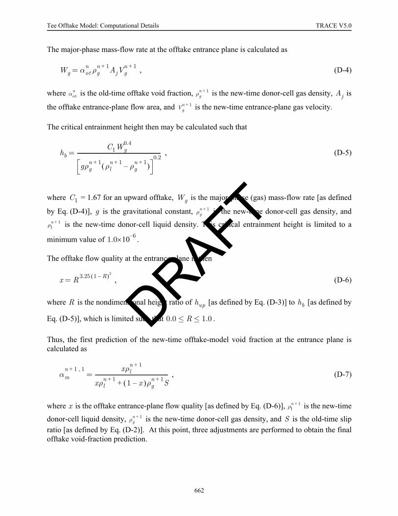
Tee Offtake Model: Computational Details TRACE V5.0
The major-phase mass-flow rate at the offtake entrance plane is calculated as
, (D-4)
where is the old-time offtake void fraction, is the new-time donor-cell gas density, is
the offtake entrance-plane flow area, and is the new-time entrance-plane gas velocity.
The critical entrainment height then may be calculated such that
, (D-5)
where = 1.67 for an upward offtake, is the major-phase (gas) mass-flow rate [as defined
by Eq. (D-4)], is the gravitational constant, is the new-time donor-cell gas density, and
is the new-time donor-cell liquid density. This critical entrainment height is limited to a
minimum value of .
The offtake flow quality at the entrance plane is then
, (D-6)
where is the nondimensional height ratio of [as defined by Eq. (D-3)] to [as defined by
Eq. (D-5)], which is limited such that .
Thus, the first prediction of the new-time offtake-model void fraction at the entrance plane iscalculated as
, (D-7)
where is the offtake entrance-plane flow quality [as defined by Eq. (D-6)], is the new-time
donor-cell liquid density, is the new-time donor-cell gas density, and is the old-time slipratio [as defined by Eq. (D-2)]. At this point, three adjustments are performed to obtain the finalofftake void-fraction prediction.
Wg αotn ρg
n 1+ AjVgn 1+=
αotn ρg
n 1+ Aj
Vgn 1+
hbC1Wg
0.4
gρgn 1+ ρl
n 1+ ρgn 1+–( )
0.2----------------------------------------------------------------=
C1 Wg
g ρgn 1+
ρln 1+
1.0 6–×10
x R 3.25 1 R–( )2
=
R hup hb
0.0 R 1.0≤ ≤
αmn 1 1,+ xρl
n 1+
xρln 1+ 1 x–( )ρg
n 1+ S+--------------------------------------------------------=
x ρln 1+
ρgn 1+ S
DRAFT
662

TRACE V5.0 Tee Offtake Model: Computational Details FOOBAR1234
Tee O
fftake M
odel: C
omputational
First, if the liquid level in the main-tube-junction cell is above the offtake entrance plane, theofftake void fraction predicted by Eq. (D-7) is modified to ensure that it approaches the value ofthe void fraction in the main-tube-junction cell as the liquid level reaches the top of the main-tube-junction cell. This interpolation is performed linearly with the main-tube-junction cell liquiddepth, , such that
, (D-8)
where
, (D-9)
is the main-tube-junction cell liquid depth, is the main-tube-junction cell average
diameter, is the critical main-tube-junction cell liquid depth at which the liquid level just
reaches the offtake entrance plane, is the first offtake void-fraction prediction [as defined
by Eq. (D-7)], and is the new-time main-tube-junction cell void fraction.
Next, this offtake void-fraction result is weighted using the horizontal stratified-flow weightingfactor to ensure that the offtake void fraction tends toward the main-tube-junction cell voidfraction as the flow, moves away from a stratified-flow regime such that
, (D-10)
where is the horizontal-flow weighting factor, is the second offtake void-fraction
prediction [as defined by Eq. (D-8)], and is the new-time main-tube-junction cell voidfraction.
Finally, the offtake void-fraction prediction is limited to ensure that the volume of liquidentrained does not exceed the volume that exists in the main-tube-junction cell such that
, (D-11)
where is the third offtake void-fraction prediction [as defined by Eq. (D-10)] and isthe new-time main-tube-junction cell void fraction. At this point, the new-time offtake voidfraction, , is returned to the calling routine.
h1
αmn 1 2,+
fαmn 1 1,+
1 f–( )α1n 1++=
fh1 D1–hc D1–------------------=
h1 D1
hc
αmn 1 1,+
α1n 1+
αmn 1 3,+
WFHF αmn 1 2,+
1 WFHF–( )α1n 1++=
WFHF αmn 1 2,+
α1n 1+
αotn 1+ Max αm
n 1 3,+α1
n 1+,⎝ ⎠⎛ ⎞=
αmn 1 3,+
α1n 1+
αotn 1+
DRAFT
663

Tee Offtake Model: Computational Details TRACE V5.0
Side-Oriented Offtake
For the case of the side-oriented offtake, the major-flow component may be either the gas phaseor the liquid phase. When the liquid level in the main tube is below the offtake center, the gasphase is the major-flow component and liquid entrainment may occur. However, if the liquidlevel in the main tube is above the offtake center, the liquid phase becomes the major-flowcomponent and gas entrainment may be possible. The following description first details the caseof when the gas phase is the major-flow component and liquid entrainment may occur, and thenoutlines the case when the liquid phase is the major-flow component and gas entrainment may bepossible.
Liquid Entrainment Scenario
For the case of the side-oriented offtake with a gas major-flow component (the case of possibleliquid entrainment), the actual characteristic height is approximated as
, (D-12)
where is the main-tube-junction cell liquid depth and is the main-tube-junction cell
average diameter. Notice that for this offtake configuration, is a negative value, which later
causes the nondimensional height ratio, , to also be negative in value.
The major-phase mass-flow rate at the offtake entrance plane is calculated as
, (D-13)
where is the old-time offtake void fraction, is the new-time donor-cell gas density, is
the offtake entrance-plane flow area, and is the new-time entrance-plane gas velocity.
The critical entrainment height then may be calculated such that
, (D-14)
where = 0.69 for a side-oriented offtake with a gas major-flow component, is the major-
phase (gas) mass-flow rate [as defined by Eq. (D-13)], is the gravitational constant, is the
new-time donor-cell gas density, and is the new-time donor-cell liquid density. This critical
hsd h1 0.5D1–=
h1 D1
hsd
R
Wg αotn ρg
n 1+ AjVgn 1+=
αotn ρg
n 1+ Aj
Vgn 1+
hbC1Wg
0.4
gρgn 1+ ρl
n 1+ ρgn 1+–( )
0.2----------------------------------------------------------------=
C1 Wg
g ρgn 1+
ρln 1+
DRAFT
664

TRACE V5.0 Tee Offtake Model: Computational Details FOOBAR1234
Tee O
fftake M
odel: C
omputational
entrainment height is limited to be no less than the larger of and [seeEq. (D-1)].
The offtake flow quality at the entrance plane is then
, (D-15)
where
, (D-16)
is the nondimensional height ratio of [as defined by Eq. (D-12)] to [as defined by
Eq. (D-14)], is the new-time donor-cell liquid density, is the new-time donor-cell gasdensity, and = 1.00 for liquid entrainment.
Thus, the first prediction of the new-time offtake-model void fraction at the entrance plane iscalculated as
, (D-17)
where is the offtake entrance-plane flow quality [as defined by Eq. (D-15)], is the new-
time donor-cell liquid density, is the new-time donor-cell gas density, and is the old-timeslip ratio [as defined by Eq. (D-2)]. At this point, three adjustments are performed to obtain thefinal offtake void-fraction prediction.
First, if the liquid level in the main-tube-junction cell is between the bottom and the centerline ofthe offtake entrance, the offtake void fraction predicted by Eq. (D-17) is modified to ensure that itapproaches the value of the void fraction in the main-tube-junction cell as the diameter of theofftake approaches the diameter of the main-tube-junction cell. This interpolation is performedlinearly with the main-tube-junction cell liquid depth, such that
, (D-18)
where
1.0 6–×10 0.5Dot
x xo1 C2R+( )
1 0.5R 1 R+( )xo1 R–( )–[ ]
0.5=
xo1.15
1ρl
n 1+
ρgn 1+
------------+
--------------------------=
R hsd hb
ρln 1+ ρg
n 1+
C2
αmn 1 1,+ xρl
n 1+
xρln 1+ 1 x–( )ρg
n 1+ S+--------------------------------------------------------=
x ρln 1+
ρgn 1+ S
h1
αmn 1 2,+
fαmn 1 1,+
1 f–( )α1n 1++=
DRAFT
665

Tee Offtake Model: Computational Details TRACE V5.0
, (D-19)
and where is the critical main-tube-junction cell liquid depth at which the liquid level just
reaches the offtake entrance, is the main-tube-junction cell liquid depth, is the first
offtake void-fraction prediction [as defined by Eq. (D-17)], and is the new-time main-tube-junction cell void fraction.
Next, this offtake void-fraction result is weighted using the horizontal stratified-flow weightingfactor to ensure that the offtake void fraction tends toward the main-tube-junction cell voidfraction as the flow moves away from a stratified-flow regime such that
, (D-20)
where is the horizontal-flow weighting factor, is the second offtake void-fraction
prediction [as defined by Eq. (D-18)], and is the new-time main-tube-junction cell voidfraction.
Finally, the offtake void-fraction prediction is limited to ensure that the volume of liquidentrained does not exceed the volume that exists in the main-tube-junction cell such that
, (D-21)
where is the third offtake void-fraction prediction [as defined by Eq. (D-20)] and isthe new-time main-tube-junction cell void fraction. At this point, the new-time offtake voidfraction, , is returned to the calling routine.
Gas Entrainment Scenario
For the case of the side-oriented offtake with a liquid major-flow component (the case of possiblegas entrainment), the actual characteristic height is approximated as
, (D-22)
where is the main-tube-junction cell liquid depth and is the main-tube-junction cellaverage diameter.
fhch1-----=
hc
h1 αmn 1 1,+
α1n 1+
αmn 1 3,+
WFHF αmn 1 2,+
1 WFHF–( ) α1n 1++·=
WFHF αmn 1 2,+
α1n 1+
αotn 1+ Max αm
n 1 3,+α1
n 1+,⎝ ⎠⎛ ⎞=
αmn 1 3,+
α1n 1+
αotn 1+
hsd h1 0.5D1–=
h1 D1
DRAFT
666

TRACE V5.0 Tee Offtake Model: Computational Details FOOBAR1234
Tee O
fftake M
odel: C
omputational
The major-phase mass-flow rate at the offtake entrance plane is calculated as
, (D-23)
where is the old-time offtake void fraction, is the new-time donor-cell liquid density,
is the offtake entrance-plane flow area, and is the new-time entrance-plane liquid velocity.
The critical entrainment height then may be calculated such that
, (D-24)
where = 0.75 for a side-oriented offtake with a liquid major-flow component, is the
major-phase (liquid) mass-flow rate [as defined by Eq. (D-23)], is the gravitational constant, is the new-time donor-cell liquid density, and is the new-time donor-cell gas density.
This critical entrainment height is limited to be no less than the larger of and [see Eq. (D-1)].
The offtake flow quality at the entrance plane is then
(D-25)
for the range
,
where
, (D-26)
is the nondimensional height ratio of [as defined by Eq. (D-22)] to [as defined by
Eq. (D-24)], is the new-time donor-cell liquid density, is the new-time donor-cell gasdensity, and = 1.09 for gas entrainment.
Wl 1 αotn–( )ρl
n 1+ AjVln 1+=
αotn ρl
n 1+ Aj
Vln 1+
hbC1Wl
0.4
gρln 1+ ρl
n 1+ ρgn 1+–( )
0.2----------------------------------------------------------------=
C1 Wl
gρl
n 1+ ρgn 1+
1.0 6–×10 0.5Dot
x xo1 C2R+( )
1 0.5R 1 R+( )xo1 R–( )–[ ]
0.5=
0.0 R 0.9≤ ≤
xo1.15
1ρl
n 1+
ρgn 1+
------------+
--------------------------=
R hsd hb
ρln 1+ ρg
n 1+
C2
DRAFT
667

Tee Offtake Model: Computational Details TRACE V5.0
In Eq. (D-25), as approaches 1, approaches 0 very rapidly. To avoid an exponentialapproach toward zero, the term was replaced with a linear function for the range
, resulting in the following formulation for flow quality:
(D-27)
for the range
,
where is defined by Eq. (D-26), = 1.09 for gas entrainment, and is again thenondimensional height ratio.
Thus, the first prediction of the new-time offtake-model void fraction at the entrance plane iscalculated as
, (D-28)
where is the offtake entrance-plane flow quality [as defined by Eq. (D-25) or Eq. (D-27)],
is the new-time donor-cell liquid density, is the new-time donor-cell gas density, and S is theold-time slip ratio [as defined by Eq. (D-2)]. At this point, three adjustments are performed toobtain the final offtake void-fraction prediction.
First, if the liquid level in the main-tube-junction cell is between the centerline and the top of theofftake entrance, the offtake void fraction predicted by Eq. (D-28) is modified to ensure that itapproaches the value the of the void fraction in the main-tube-junction cell as the diameter of theofftake approaches the diameter of the main-tube-junction cell. This interpolation is performedlinearly with the main-tube-junction cell liquid depth, such that
, (D-29)
where
, (D-30)
R xR 1 R+( )
0.9 R 1.0≤ ≤
x 10.0xo1 C2R+( )
1 0.855xo0.1–[ ]
0.5R 1.0–( )–=
0.9 R 1.0≤ ≤
xo C2 R
αmn 1 1,+ xρl
n 1+
xρln 1+ 1 x–( )ρg
n 1+ S+--------------------------------------------------------=
x ρln 1+
ρgn 1+
h1
αmn 1 2,+
fαmn 1 1,+
1 f–( )α1n 1++=
fD1 hc–D1 h1–------------------=
DRAFT
668

TRACE V5.0 Tee Offtake Model: Computational Details FOOBAR1234
Tee O
fftake M
odel: C
omputational
is the main-tube-junction cell average diameter, is the critical main-tube-junction cell
liquid depth at which the liquid level just reaches the offtake entrance, is the main-tube-
junction cell liquid depth, is the first offtake void-fraction prediction [as defined by
Eq. (D-28)], and is the new-time main-tube-junction cell void fraction.
Next, this offtake void-fraction result is weighted using the horizontal stratified-flow weightingfactor to ensure that the offtake void fraction tends toward the main-tube-junction cell voidfraction as the flow moves away from a stratified-flow regime such that
, (D-31)
where is the horizontal-flow weighting factor, is the second offtake void-fraction
prediction [as defined by Eq. (D-29)], and is the new-time main-tube-junction cell voidfraction.
Finally, the offtake void-fraction prediction is limited to ensure that the volume of gas entraineddoes not exceed the volume that exists in the main-tube-junction cell such that
, (D-32)
where is the third offtake void-fraction prediction [as defined by Eq. (D-31)] and isthe new-time main-tube-junction cell void fraction. At this point, the new-time offtake voidfraction, , is returned to the calling routine.
Downward Offtake
For the case of the downward offtake, the major-flow component is the liquid phase. The actualcharacteristic height for the downward offtake is approximated as
, (D-33)
where is the main-tube-junction cell liquid depth.
The major-phase mass-flow rate at the offtake entrance plane is calculated as
, (D-34)
D1 hc
h1
αmn 1 1,+
α1n 1+
αmn 1 3,+
WFHF αmn 1 2,+
1 WFHF–( )α1n 1++=
WFHF αmn 1 2,+
α1n 1+
αotn 1+ Min αm
n 1 3,+α1
n 1+,⎝ ⎠⎛ ⎞=
αmn 1 3,+
α1n 1+
αotn 1+
hdn h1=
h1
Wl 1 αotn–( )ρl
n 1+ AjVln 1+=
DRAFT
669

Tee Offtake Model: Computational Details TRACE V5.0
where is the old-time offtake void fraction, is the new-time donor-cell liquid density,
is the offtake entrance-plane flow area, and is the new-time entrance-plane liquid velocity.
The critical entrainment height then may be calculated such that
, (D-35)
where = 1.50 for a downward offtake, is the major-phase (liquid) mass-flow rate [as
defined by Eq. (D-34)], is the gravitational constant, is the new-time donor-cell liquid
density, and is the new-time donor-cell gas density. This critical entrainment height is
limited to a minimum value of .
The offtake flow quality at the entrance plane is then
(D-36)
for the range
,
where
, (D-37)
is the nondimensional height ratio of [as defined by Eq. (D-33)] to [as defined by
Eq. (D-35)], is the new-time donor-cell liquid density, and is the new-time donor-cellgas density.
In Eq. (D-36), as approaches 1, approaches 0 very rapidly. To avoid an exponentialapproach toward zero, the term was replaced with a linear function for the range
resulting in the following formulation for flow quality:
αotn ρl
n 1+ Aj
Vln 1+
hbC1Wl
0.4
gρln 1+ ρl
n 1+ ρgn 1+–( )
0.2----------------------------------------------------------------=
C1 Wl
g ρln 1+
ρgn 1+
1.0 6–×10
x xo2.5R 1 0.5R 1 R+( )xo
1 R–( )–[ ]0.5
=
0.0 R 0.9<≤
xo1.15
1ρl
n 1+
ρgn 1+
------------+
--------------------------=
R hdn hb
ρln 1+ ρg
n 1+
R xR 1 R+( )
0.9 R 1.0≤ ≤
DRAFT
670
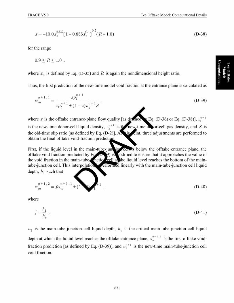
TRACE V5.0 Tee Offtake Model: Computational Details FOOBAR1234
Tee O
fftake M
odel: C
omputational
(D-38)
for the range
,
where is defined by Eq. (D-35) and is again the nondimensional height ratio.
Thus, the first prediction of the new-time model void fraction at the entrance plane is calculated as
, (D-39)
where is the offtake entrance-plane flow quality [as defined by Eq. (D-36) or Eq. (D-38)],
is the new-time donor-cell liquid density, is the new-time donor-cell gas density, and isthe old-time slip ratio [as defined by Eq. (D-2)]. At this point, three adjustments are performed toobtain the final offtake void-fraction prediction.
First, if the liquid level in the main-tube-junction cell is below the offtake entrance plane, theofftake void fraction predicted by Eq. (D-39) is modified to ensure that it approaches the value ofthe void fraction in the main-tube-junction cell as the liquid level reaches the bottom of the main-tube-junction cell. This interpolation is performed linearly with the main-tube-junction cell liquiddepth, such that
, (D-40)
where
, (D-41)
is the main-tube-junction cell liquid depth, is the critical main-tube-junction cell liquid
depth at which the liquid level reaches the offtake entrance plane, is the first offtake void-
fraction prediction [as defined by Eq. (D-39)], and is the new-time main-tube-junction cellvoid fraction.
x 10.0xo2.5R 1 0.855xo
0.1–[ ]0.5
R 1.0–( )–=
0.9 R 1.0≤ ≤
xo R
αmn 1 1,+ xρl
n 1+
xρln 1+ 1 x–( )ρg
n 1+ S+--------------------------------------------------------=
x ρln 1+
ρgn 1+ S
h1
αmn 1 2,+
fαmn 1 1,+
1 f–( ) α1n 1++=
fh1hc-----=
h1 hc
αmn 1 1,+
α1n 1+
DRAFT
671

Tee Offtake Model: Computational Details TRACE V5.0
Next, this offtake void-fraction result is weighted using the horizontal stratified-flow weightingfactor to ensure that the offtake void fraction tends toward the main-tube-junction cell voidfraction as the flow moves from a stratified-flow regime such that
, (D-42)
where is the horizontal-flow weighting factor, is the second offtake void-fraction
prediction [as defined by Eq. (D-40)], and is the new-time main-tube-junction cell voidfraction.
Finally, the offtake void-fraction prediction is limited to ensure that the volume of gas entraineddoes not exceed the volume that exists in the main-tube-junction cell such that
, (D-43)
where is the third offtake void-fraction prediction [as defined by Eq. (D-42)] and isthe new-time main-tube-junction cell void fraction. At this point, the new-time, offtake voidfraction, , is returned to the calling routine.
αmn 1 3,+
WFHF αmn 1+ 2,
1 WFHF–( ) α1n 1–+·=
WFHF αmn 1 2,+
α1n 1+
aotn 1+ Min αm
n 1 3,+α1
n 1+,⎝ ⎠⎛ ⎞=
αmn 1 3,+
α1n 1+
αotn 1+
DRAFT
672