Embed Size (px)
Citation preview

Equation Chapter 1 Section 1
Trabajo Fin de Máster
Máster en Diseño Avanzado en Ingeniería
Mecánica
Numerical Computation of the Unsteady Linearized
Potential Flow past Airfoils in Compressible
Subsonic Regime by Finite Differences Methods
Autor: Manuel Colera Rico
Tutor: Miguel Pérez-Saborid Sánchez-Pastor
Dep. Ingeniería Aeroespacial y Mecánica de Fluidos
Escuela Técnica Superior de Ingeniería
Universidad de Sevilla
Sevilla, 2016


Trabajo Fin de Máster
Máster en Diseño Avanzado en Ingeniería Mecánica
Numerical Computation of the Unsteady Linearized
Potential Flow past Airfoils in Compressible
Subsonic Regime by Finite Differences Methods
Autor:
Manuel Colera Rico
Tutor:
Miguel Pérez-Saborid Sánchez-Pastor
Profesor Titular
Dep.Ingeniería Aeroespacial y Mecánica de Fluidos
Escuela Técnica Superior de Ingeniería
Universidad de Sevilla
Sevilla, 2016


A mi familia, en especial, a mis
padres, y a mis amigos

Acknowledgements
I would like to express my gratitude to professor Miguel Perez-Saborid for initiatingme in the world of computational fluid dynamics during the last years, and for his greatdedication and advice along this work.
I also thank my parents for their support and their magnificent guidance —both intechnical and human aspects— during all these years, as well as my aunt Inma for herbrilliant pieces of advice about writing technical essays.
Finally, I am grateful to all my friends for making the University one of my very bestexperiences.
The author


Contents
Introduction 3
Motivation, aims and applications . . . . . . . . . . . . . . . . . . . . . . . . . . 3
Structure and main contributions . . . . . . . . . . . . . . . . . . . . . . . . . . . 6
1. General equations and considerations 7
1.1. Introduction . . . . . . . . . . . . . . . . . . . . . . . . . . . . . . . . . . . . 7
1.2. Linearized potential flow equations . . . . . . . . . . . . . . . . . . . . . . . 7
1.3. Lift, pitching moment and other generalized forces . . . . . . . . . . . . . . 10
1.4. Finite differences for non-uniform meshes . . . . . . . . . . . . . . . . . . . 11
1.5. Non-reflecting boundary conditions . . . . . . . . . . . . . . . . . . . . . . . 12
2. Modified Hariharan-Ping-Scott method 15
2.1. Introduction . . . . . . . . . . . . . . . . . . . . . . . . . . . . . . . . . . . . 15
2.2. Description of the method . . . . . . . . . . . . . . . . . . . . . . . . . . . . 16
2.2.1. Main concepts . . . . . . . . . . . . . . . . . . . . . . . . . . . . . . 16
2.2.2. Derivation of A0 and A1 . . . . . . . . . . . . . . . . . . . . . . . . 19
2.2.3. Efficient scheme implementation. Summary of all the steps . . . . . 23
2.3. Results . . . . . . . . . . . . . . . . . . . . . . . . . . . . . . . . . . . . . . . 25
2.3.1. Wagner’s problem . . . . . . . . . . . . . . . . . . . . . . . . . . . . 27
2.3.2. Theodorsen’s problem . . . . . . . . . . . . . . . . . . . . . . . . . . 28
2.3.3. Kussner’s problem . . . . . . . . . . . . . . . . . . . . . . . . . . . . 31
2.4. Convergence and stability comparisons between the modified and the orig-inal Hariharan-Ping-Scott methods . . . . . . . . . . . . . . . . . . . . . . . 32
1

2 Contents
2.5. Convergence and efficiency comparison between the modified Hariharan-Ping-Scottand the modified Hernandes-Soviero methods . . . . . . . . . . . . . . . . . 34
2.6. Wake patterns calculation . . . . . . . . . . . . . . . . . . . . . . . . . . . . 38
3. Coupling of airfoil dynamics with the modified Hariharan-Ping-Scottmethod 41
3.1. Introduction . . . . . . . . . . . . . . . . . . . . . . . . . . . . . . . . . . . . 41
3.2. Description of the coupled Hariharan-Ping-Scott method . . . . . . . . . . . 42
3.2.1. Main concepts . . . . . . . . . . . . . . . . . . . . . . . . . . . . . . 42
3.2.2. Computation of the first instants . . . . . . . . . . . . . . . . . . . . 45
3.2.3. Efficient scheme implementation. Summary of all the steps . . . . . 46
3.3. Results . . . . . . . . . . . . . . . . . . . . . . . . . . . . . . . . . . . . . . . 48
3.3.1. Flutter of a rigid airfoil . . . . . . . . . . . . . . . . . . . . . . . . . 48
3.3.2. Flutter of a cantilevered flexible plate . . . . . . . . . . . . . . . . . 51
3.3.3. Response to a vertical sharp-edge gust . . . . . . . . . . . . . . . . . 57

Introduction
Motivation, aims and applications
The interest for unsteady aerodynamic flows has increased in the recent years due toits many applications. For example, in aeronautics it is of primordial importance to knowthe extra loads over an aeroplane that suddenly changes its angle of attack, enters in a gustor goes into a turbulence zone. In addition, many aeroelastic problems can appear suchas the divergence and the flutter of wings or other aerodynamic surfaces. In biomedicine,snoring problems are studied by analysing the unsteady oscillations of the vocal chordsproduced by the air that passes through the throat. Aeroelastic problems are also ofinterest in civil engineering, where wind can cause flutter in tall bridges and buildings ashappened, for example, in the famous case of the failure of the Tacoma Bridge (figure 1).
Figure 1: Flutter problem at the Tacoma Bridge, that caused its destruction later.Photography obtained from
https://en.wikipedia.org/wiki/Tacoma Narrows Bridge (1940).
Usually, many of those phenomena (such as snoring and wing flutter) are not modelleddirectly as three-dimensional problems. Instead, according to the strip theory [9], thecorresponding entity (the vocal cords or the wing) is divided into cross sections that arestudied as if they were subject to a two-dimensional flow. Using this approximation, thelinearized potential theory for flows past airfoils was developed around 1940. This theory
3

4 Introduction
yields simple equations whose physical meaning is very clear. However, this transparencywas soon lost since, due to the absence of efficient computers in those times, the equationshad to be solved analytically —usually in the frequency domain—, leading to tediousmathematical developments whose physical meaning is difficult to grasp and disorientatethe interested students, especially when air compressibility is taken into account. Further-more, many of those developments —which are still used as a reference in the specializedliterature— are only valid for particular cases such as harmonic motion, sudden changesin the angle of attack, sharp edge gusts, etc.
Since computers have experienced a great development in the last years, some effortshave been made to solve numerically the linearized, unsteady potential equations in aneasier and more direct way, which is valid for any motion of the airfoil and uses the morephysically intuitive time domain approach. For example, Katz and Plotkin [15] developeda marching-time vortex-lattice method for incompressible flow that was able to calculatethe forces over an airfoil when its motion was known, and Hernandes and Soviero [12][13]presented a similar method suitable for compressible flow. Both methods were studiedand improved by Colera and Perez-Saborid [6], who proposed two truncation algorithmsin order to reduce their computational cost. These authors also coupled the equations ofthe vortex-lattice methods with those of the airfoil dynamics for studying problems werethe airfoil motion is the unknown as happens, for example, in the problem of flutter.
Although the Hernandes-Soviero method is precise and valid for general two-dimensionalproblems, it presents some drawbacks:
A good comprehension of not well-known aspects such as the induced velocity fieldof unsteady compressible vortexes, the piston theory and the auto-induced velocitiesof an unsteady vortex in supersonic flow is required.
The method is constructed by means of the unsteady compressible vortex, a funda-mental solution that presents a lack of physical meaning, as pointed in [6].
It is a marching-time method which has to keep track of the solutions correspondingto many previous times in order to compute the solution at some given instant.Thus, it can run very slowly even with the truncation method developed in [6].
Its extension to the three-dimensional regime is not clear, despite some works havebeen done on the matter [19].
The disadvantages that vortex-lattice methods pose in the case of compressible un-steady flows past airfoils have motivated the consideration in this work of an alternativemarching-time method that is not based on the use of unsteady compressible vortexesor any other fundamental solutions, but on discretizing the differential equations of thelinearized potential flow theory directly by finite differences. Originally, this method wasproposed by Hariharan, Ping and Scott [11], who used an uniform grid to mesh the fluiddomain and an explicit time integration scheme. Despite providing good accuracy and be-ing easy to understand and implement, this method, as presented by these authors, makesnecessary to use a very thin mesh to get good results, as well as a very small time stepin order to avoid instabilities. Also, the method was implemented for the case when themotion of the airfoil is given, but not when it is just the unknown as in flutter problems.
All of this has motivated the present work, whose main objectives are:

Motivation, aims and applications 5
To propose a modification for the Hariharan-Ping-Scott method that uses a non-uniform mesh and an implicit time integration scheme, leading to better accuracyand stability. This modification will be just named as modified Hariharan-Ping-Scottmethod in this work, and its efficiency will be compared with the Hernandes-Sovierovortex-lattice modified with the truncation algorithm proposed by Colera and Perez-Saborid [6]. Similarly, the latter method will be named as modified Hernandes-Soviero method in this work.
To couple the modified Hariharan-Ping-Scott method with the airfoil dynamics inorder to compute its motion when it is unknown. This coupling algorithm will benamed coupled Hariharan-Ping-Scott method along this work.
As applications of the above mentioned methods, some results of interest that are verydifficult to obtain analytically have been computed like, for example, the extra lift thatappears after a sudden change of the angle of attack or after a sharp-edge gust, whichcould be of interest for structural calculations. Also, the wake evolution, that can seri-ously affect the behaviour of aeroplanes or turbomachine blades, has been computed forthe two-dimensional case. The flutter point of rigid and flexible airfoils has also been con-sidered and, apparently, this is first self-consistent numerical analysis of the compressible,linearized coupled dynamics of the fluid-airfoil system carried out in the literature. Fur-thermore, for the flutter of a flexible airfoil in compressible flow, no references have beenfound in the available literature to make comparisons with, thus, the results presentedhere for that case are original or not well-known.
(a) (b)
Figure 2: Asymmetric flutter mode in a glider (a) and wake after an aeroplane that canseriously affect the control of incoming ones (b).
The methods analysed in this work can be easily and efficiently implemented withprograms like Matlab, which has simple syntax rules, is well-known by students and hasmany mathematical libraries that allow a friendlier implementation. Also, they makeuse of the physics beyond the basic equations of the unsteady linearized potential theory,never leaving the time domain. Thus, they are very intuitive (unlike the classical frequencydomain approach) and can be very useful for teaching applications. Also, since they areefficient, precise and permit the calculation of many variables of interest, they can be usedfor the preliminary design of wings and helicopter blades or for any other situation where

6 Introduction
the computation based on CFD commercial programs is too expensive for the requiredprecision.
Finally, this work is a way to put into practice some concepts learned in the MasterDegree in Advanced Design in Mechanical Engineering, such as linear waves in gas dy-namics, classic mechanics and computational methods (sparse matrixes, LU factorizationand BDF for ordinary differential equations).
Structure and main contributions
This work is mainly structured in three chapters. In the first one, some general conceptsare to be introduced such as the principal equations of the linearized potential theory offlows past airfoils, some finite differences formulas for non-uniform meshes and a non-reflecting boundary condition for the convected wave equation.
In the second chapter, those general concepts are to be used in order to explain themodified Hariharan-Ping-Scott method. As commented before, this method differs fromthe original one in that it uses a non-uniform grid and an implicit time integration scheme,being then more accurate and stable. These improvements are original and therefore theyconstitute one of the main contributions of this work. Some problems of interest willbe solved with the method and its efficiency and convergence will be compared with theHernandes-Soviero method’s.
In the third chapter, the modified method is to be coupled with the airfoil dynamicsin order to compute its motion in the case in which it is the unknown. Again, thiscoupling method is original and therefore it is another contribution of this work. Withthe coupled method, some problems related to the flutter of rigid and flexible airfoils andto the response to a gust are to be solved. As pointed before, no results have been foundin the available literature to compare with the obtained ones in the case of the flutter ofa flexible airfoil. Hence, those results are original or not well-known and are one of themain contributions of this work as well.
Finally, the bibliography consulted for this work is included.

Chapter 1
General equations andconsiderations
1.1. Introduction
In this chapter some general ideas are to be introduced briefly before approaching theexplanation of the numerical methods in the following chapters. First, some simplificationsinvolving the fluid and the airfoil and also the equations that govern the flow are shown insection 1.2. Second, the calculation of the lift, the pitching moment and other generalizedforces over the airfoil by means of the fluid variables is explained in section 1.3. Later,some finite differences formulas for non-uniform meshes that will be implemented in thenumerical methods are derived in section 1.4. Finally, an additional boundary conditionfor finite domains is obtained in section 1.5 following the same reasoning that Hariharan,Ping and Scott [11].
1.2. Linearized potential flow equations
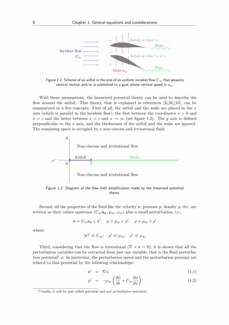
Consider an airfoil —which is two-dimensional by definition— in the sine of an hor-izontal, constant and uniform flow of speed U∞ that presents vertical motion and/or issubmitted to a gust whose vertical speed is wg (as shown in figure 1.1), and assume thefollowing hypothesises, valid for the most part of practical cases:
The Reynolds number based on the chord lenght c of the airfoil and the propertiesof the fluid upstream is very high, so viscous effects can be neglected except in theboundary layer of the airfoil and in the wake.
Gravity forces and heat transfer are neglected as well.
The amplitude of the airfoil motion and the gust intensity are small, i.e., their speedsare much lower than U∞ and the displacements of the airfoil are much lower than c.
The airfoil’s thickness is much lower than its chord c.
The boundary layer of the airfoil remains adhered to it.
7
8 Chapter 1. General equations and considerations
Airfoil at time t1
Airfoil at time t2 6= t1
Gust wg
Incident flow
U∞
Wake
Wake
Figure 1.1: Scheme of an airfoil in the sine of an uniform incident flow U∞ that presentsvertical motion and/or is submitted to a gust whose vertical speed is wg.
With these assumptions, the linearized potential theory can be used to describe theflow around the airfoil. This theory, that is explained in references [3],[6],[10], can besummarized in a few concepts. First of all, the airfoil and the wake are placed in the xaxis (which is parallel to the incident flow), the first between the coordinates x = 0 andx = c and the latter between x = c and x → ∞ (see figure 1.2). The y axis is definedperpendicular to the x axis, and the thicknesses of the airfoil and the wake are ignored.The remaining space is occupied by a non-viscous and irrotational fluid.
y
Airfoil Wake
c0x−
Non-viscous and irrotational flow
Non-viscous and irrotational flow
Figure 1.2: Diagram of the flow field simplification made by the linearized potentialtheory.
Second, all the properties of the fluid like the velocity v, pressure p, density ρ, etc. arewritten as their values upstream (U∞ux, p∞, ρ∞) plus a small perturbation, i.e.:
v = U∞ex + v′; p = p∞ + p′; ρ = ρ∞ + ρ′
where:|v|′ � U∞; p′ � p∞; ρ′ � ρ∞
Third, considering that the flow is irrotational (∇ × v = 0), it is shown that all theperturbation variables can be extracted from just one variable, that is the fluid perturba-tion potential1 φ. In particular, the perturbation speed and the perturbation pressure arerelated to that potential by the following relationships:
v′ = ∇φ (1.1)
p′ = −ρ∞(∂φ
∂t+ U∞
∂φ
∂x
)(1.2)
1Usually, it will be just called potential and not perturbation potential.

1.2. Linearized potential flow equations 9
In unsteady problems, the potential is antisymmetric respect to the x axis (inducingan antisymmetric perturbation velocity v′ as well), being continuous at x < 0, y = 0 andpresenting a jump across the line occupied by the airfoil and the wake (x > 0, y = 0).Thus, it is only necessary to calculate the potential in the upper half plane (y > 0).
It has to be noticed that, due to that antisymmetry, φ(x, 0+) = φ(x, 0−) = 0 at leastwhen x < 0. However, it is important to remark that the latter relation can be extendedto the point x = 0, because φ is continuous in that point. Indeed, there is a well-knownleading edge suction, that takes place at x = y = 0, and is characterized by a vortex densityγ that behaves as 1/
√x. It can be shown [6] that this vortex density is proportional to the
horizontal perturbation velocity u = ∂φ/∂x so, in the vecinities of the point x = y = 0,φ has to behave as
√x, as shown in figure 1.3. Therefore, φ is continuous at x = y = 0
(although it presents an infinite slope there) and it is possible to say that:
φ(x, 0+) = φ(x, 0−) = 0; x ≤ 0 (1.3)
ε� cx
∂φ∂x (t, x, 0+)
0
∼ 1√x
ε� cx
φ(t, x, 0+)
0
∼√x
Figure 1.3: Illustration of the asymptotic behaviour of ∂φ/∂x and φ nearby x = y = 0due to the presence of the well-known leading edge suction. As can be seen, the
mentioned suction does not imply any discontinuity for φ in that point.
The equation that governs the potential φ in the fluid domain is the convected waveequation: (
∂
∂t+ U∞
∂
∂x
)2
φ = a2∞∇2φ (1.4)
where a∞ is the upstream sound speed. In order to develop the numerical code presentedin this work, it is convenient to rewrite the latter equation in the following way:
∂2φ
∂t2= −2U∞
∂2φ
∂t ∂x+(a2∞ − U2
∞) ∂2φ
∂x2+ a2∞∂2φ
∂z2(1.5)
The boundary conditions for the potential are:
Non-penetration of the fluid in the airfoil’s surface:
∂φ
∂z=∂zp∂t
+ U∞∂zp∂x− wg(t, x); 0 ≤ x ≤ c; y = 0+ (1.6)
where zp = zp(t, x) is the displacement of the mean geometrical line of the airfoilrespect from its steady position.

10 Chapter 1. General equations and considerations
Non-perturbed conditions at infinity:
∇φ = 0; x, y →∞; (1.7)
Kutta’s condition (applies to the wake):
∂φ
∂t+ U∞
∂φ
∂x= 0; x > c; y = 0+ (1.8)
The equations (1.5)-(1.8) are to be solved by the modified Hariharan-Ping-Scott methodpresented here to get the fluid field around the airfoil.
1.3. Lift, pitching moment and other generalized forces
Once the perturbation potential φ is found, it is of great interest to calculate theactuating lift and pitching moment2 over the airfoil.
If the upper surface of the airfoil (0 ≤ x ≤ c, y = 0+) is denoted by up, and the lowerone (0 ≤ x ≤ c, y = 0−) by down, the lift l can be expressed as:
l =
ˆ x=c
x=0
(pdown − pup
)dx
Using now the relations (1.2)-(1.3) and the fact that φ is antisymmetric, the latter equationreads as follows:
l = 2ρ∞
ˆ c
0
∂φup
∂tdx+ 2ρ∞U∞φ
up(t, x = c) (1.9)
which is the generalized Kutta-Joukowski formula.
On the other hand, the pitching moment mle over the leading edge (defined as positiveif it makes the airfoil move its leading edge down) can be obtained performing the followingintegral:
mle =
ˆ x=c
x=0
(pdown − pup
)x dx
Using again the equation (1.2) and the antisymmetry of φ, it is obtained that:
mle = 2ρ∞
ˆ c
0
∂φup
∂tx dx+ 2ρ∞U∞
ˆ c
0
∂φup
∂xx dx
For numerical reasons, it is convenient to integrate by parts the second term in the rightside of the last equation. Regarding equation (1.3), it follows that:
mle = 2ρ∞
ˆ c
0
∂φup
∂tx dx+ 2ρ∞U∞c φ
up(t, c)− 2ρ∞U∞
ˆ c
0φupdx (1.10)
Notice that using (1.10) instead of the equation before it is not necessary to derive thepotential respect to x and therefore the obtained result is more accurate.
2Actually, it is not the lift and the pitching moment, but the lift and pitching moment per unit length.However, the term per unit length will be omitted in this work.

1.4. Finite differences for non-uniform meshes 11
In some complex cases like, for example, flexible airfoils, their motion will be describedin terms of some generalized coordinates qi(t) and their corresponding shape functionsψi(x), i.e.:
zp(t, x) =∑i
ψi(x)qi(t)
In those cases, it will be of interest to calculate the generalized aerodynamic forces Qiassociated with the different coordinates. The expression of the above mentioned Qi canbe obtained giving the airfoil a virtual displacement and calculating the virtual work ofthe aerodynamic pressure. In other words:
δW =∑i
Qiδqi =
ˆ x=c
x=0
(pdown − pup
)δzpdx =
∑i
ˆ x=c
x=0
(pdown − pup
)ψiδqidx
Using the latter equation and the same procedure than the one used for calculating mle,it follows that:
Qi = 2ρ∞
ˆ c
0
∂φup
∂tψi dx+ 2ρ∞U∞ψi(c)φ
up(t, c)− 2ρ∞U∞
ˆ c
0φup
dψidx
dx (1.11)
The equations (1.9)-(1.11) will be used in the modified Hariharan-Ping-Scott methodexplained in the present work.
1.4. Finite differences for non-uniform meshes
In the method presented in this work, finite differences are to be used in a non-uniformmesh. Due to the fact that some of their expressions are not as intuitive and well-known aswhen the mesh is uniform, they are to be derived here first. In particular, the expressionsof greatest interest for the present text and that are to be shown now are the backward,forward and central approximations to the first derivative, and the central approximationto the second derivative.
Backward approximation to the first derivative
Suppose a function f(x) evaluated at three points named xi−2, xi−1 and xi (withxi−2 < xi−1 < xi), and denote f(xj), f
′(xj), f′′(xj) and so on by fj , f
′j , f
′′j , etc.
According to the Taylor expansion, if f is smooth enough it can be said that:
fi−1 = fi − f ′i∆x1 +1
2f ′′i ∆x2
1 −1
6f ′′′i ∆x3
1 +O(∆x41) (1.12)
fi−2 = fi − f ′i∆x2 +1
2f ′′i ∆x2
2 −1
6f ′′′i ∆x3
2 +O(∆x42) (1.13)
where ∆x1 = xi− xi−1 and ∆x2 = xi− xi−2. Eliminating f ′′i from the above equations, itis obtained that:
f ′i = fi∆x1 + ∆x2
∆x1∆x2− fi−1
∆x2
∆x1 (∆x2 −∆x1)+ fi−2
∆x1
∆x2 (∆x2 −∆x1)+O(∆x2
2) (1.14)
It can be checked that the error term in the latter equation involves the third derivativef ′′′i and the error terms in equations (1.12)-(1.13); thus, it disappears if f(x) is a seconddegree polynomial. In other words, the degree of precision of the formula (1.14) is 2.

12 Chapter 1. General equations and considerations
Forward approximation to the first derivative
The forward approximation gives the value of f ′i by means of the value of f in threepoints called xi, xi+1 and xi+2 (with xi < xi+1 < xi+2). It can be calculated from equation(1.14) replacing xi−1 by xi+1 and xi−2 by xi+2, following that:
f ′i = −fi∆x1 + ∆x2
∆x1∆x2+ fi+1
∆x2
∆x1 (∆x2 −∆x1)− fi+2
∆x1
∆x2 (∆x2 −∆x1)+O(∆x2
2) (1.15)
where, now, ∆x1 and ∆x2 represent xi+1 − xi and xi+2 − xi, respectively. Again, thisformula has an accuracy degree equal to 2.
Centered approximation to the first derivative
In this case, f is evaluated at xi−1, xi and xi+1 (with xi−1 < xi < xi+1), and the aimis to compute f ′i . Proceeding again with the Taylor series, it can be written that:
fi−1 = fi − f ′i∆x− +1
2f ′′i ∆x2
− −1
6f ′′′i ∆x3
− +O(∆x4−) (1.16)
fi+1 = fi + f ′i∆x+ +1
2f ′′i ∆x2
+ +1
6f ′′′i ∆x3
+ +O(∆x4+) (1.17)
where ∆x+ = xi+1 − xi and ∆x− = xi − xi−1. Eliminating f ′′i , it follows:
f ′i ' fi+1∆x−
∆x+ (∆x+ + ∆x−)+ fi
∆x+ −∆x−∆x+∆x−
− fi−1∆x+
∆x− (∆x+ + ∆x−)+
O(∆x2+,∆x
2−) (1.18)
which is, as well, an approximation whose precision degree is 2.
Centered approximation to the second derivative
This approximation can be obtained if f ′i is eliminated from the system (1.16)-(1.17),leading to:
f ′′i = fi+12
∆x+(∆x+ + ∆x−)− fi
2
∆x+∆x−+ fi−1
2
∆x−(∆x+ + ∆x−)+
O(∆x+,∆x−) (1.19)
which is, in the general case of non-uniform mesh (∆x− 6= ∆x+), an approximation withprecision degree equal to 2. It can be checked that, in the especial case of uniform mesh(∆x− = ∆x+), the terms involving f ′′′i in equations (1.16)-(1.17) cancel themselves whenoperating in order to obtain equation (1.19), and the error term in the latter becomesO(∆x2
+,∆x2−), as expected.
1.5. Non-reflecting boundary conditions
According to equation (1.4), the airfoil can be seen as a source of waves whose focusconvects downstream with velocity U∞ and whose front propagates with velocity a∞ re-spect to that focus [6], as seen in figure 1.4. Since the real domain is infinite, these waves

1.5. Non-reflecting boundary conditions 13
go away from the airfoil and never come back. However, it is imposible to simulate aninfinite domain numerically, and, in practice, a big enough (but finite) domain has to beused instead. In that kind of domains, boundary condition (1.7) is not useful and hasto be substituted by another one that makes waves not to reflect when arriving at theborders.
U∞
U∞∆t
a∞∆tR∆t
x
y
θ
Figure 1.4: Wave propagation in subsonic flow. ∆t is the lapse of time between theactual time t and the instant of birth of the wave.
Looking at the variables defined in figure 1.4, it follows that:
a2∞ = R2 + U2
∞ − 2RU∞ cos θ
From this, and taking into account that R has to be positive when θ = 0, π, it is obtainedthat:
R(θ) = U∞ cos θ +
√a2∞ − U2
∞ sin2 θ (1.20)
The wavefront, given in polar coordinates (x = r cos θ, y = r sin θ) by r(θ) = R(θ)∆t,can be transformed into a cylindrical one by performing the following change of variables:
r =a∞
R(θ)r; θ = θ
In the new system, the cylindrical wavefront propagates with velocity a∞, and the far flowfield can be approximated by the Friedlander asymptotic form [18]:
φ ∼ f(t− r/a∞)√r
which verifies:∂φ
∂t+ a∞
[∂φ
∂r+φ
2r
]= 0
or, in terms of the original variables:
∂φ
∂t+ R(θ)
[∂φ
∂xcos θ +
∂φ
∂ysin θ +
φ
2r
]= 0 (1.21)
That is the differential form of the non-reflecting boundary condition that will be used inthe finite domain considered in next chapters.


Chapter 2
Modified Hariharan-Ping-Scottmethod
2.1. Introduction
It was seen in the previous chapter that, under the assumptions of the linearizedpotential theory, the airfoil and the wake could be placed in the x+ semiaxis and that allthe fluid variables could be computed from another one called the potential (denoted byφ).
Now consider a rectangle in the upper half plane that surrounds the airfoil and partof the wake, and whose vertices are far enough from the airfoil (i.e., at a distance ∼ 10 cfrom it). The main idea of the Hariharan-Ping-Scott method [11] is to mesh this rectangleinto a grid of points and to discretize there the potential flow equations. If the potential isknown at a certain instant tn in the whole mesh, all the space derivatives can be computedby finite differences and therefore the time derivates can be calculated as well through thepotential theory equations. Knowing the time derivatives, it is possible to obtain thepotential in the mesh points at the following instant tn+1, and so on until a final time tf .
That Hariharan-Ping-Scott method uses an uniform mesh and an explicit time inte-gration scheme. Although this formulation is easier to implement, it has as drawbacksthat a very thin mesh is needed in order for the results to converge (sometimes leading tocomputer memory problems), and that a very small time step size has to be taken in orderto avoid instabilities. Thus, two modifications are proposed here in order to improve thosecharacteristics. They consist, respectively, in using a non-uniform mesh that concentratesmore points where the potential presents a higher gradient —so such a thin mesh is nolonger necessary— and in employing an implicit time integration scheme —that makesthe method more stable and permits to take a much longer time step.
These modifications are to be explained first in section 2.2, where the main ideas areshown, the corresponding equations and matrixes are derived and some commentariesfor its efficient implementation are made. Second, some results for typical problems inunsteady aerodynamics are computed and compared in section 2.3 with others obtainedboth theoretically and with the Hernandes-Soviero method [12][13] modified with thetruncation algorithms proposed by Colera and Perez-Saborid [6] (that were commented
15

16 Chapter 2. Modified Hariharan-Ping-Scott method
in the introductory chapter of this text). For simplicity reasons, the latter method willbe named as modified Hernandes-Soviero method. After, a comparison of the convergenceand the stability of the original and the modified Hariharan-Ping-Scott methods is done insection 2.4. Later, a brief study of the influence of the time step size in the convergence andthe efficiency of both methods (modified Hariharan-Ping-Scott and modified Hernandes-Soviero) is done in section 2.5. Finally, some wake patterns for an harmonic movement ofthe airfoil have been computed in section 2.6.
To avoid possible confusions, it has to be pointed that, sometimes, the modifiedHariharan-Ping-Scott and the modified Hernandes-Soviero methods will be called as finitedifferences method and vortex-lattice method, respectively, because that names emphasizethe main ideas beyond them.
2.2. Description of the method
2.2.1. Main concepts
Consider a rectangular (but non-uniform) mesh like the one shown in the figure 2.1.Every point of the grid can be described by two indexes i, j, with i = 1, . . . , Nx andj = 1, . . . , Ny, and also by a single index I that moves through the grid by rows, startingfrom the bottom one, and moving to the right inside each row. The relation between Iand i, j is:
I = Nx(j − 1) + i
There are two especial values of i: one for which the corresponding value of x is equal to0 (say ile) and another one for which the corresponding value of x is equal to c (say ite).These two values represent the limits between which the airfoil is placed.
Airfoil Wakei = 1 i = ile i = ite i = Nx
j = 1
j = Ny
x ∼ −10c x = 0 x = c x ∼ 10c
y = 0
y ∼ 10c
I = 1 I = 2 I = . . .
I = Nx + 1, I = . . .
I
(i, j)U∞
Figure 2.1: Scheme of the grid employed for the method.

2.2. Description of the method 17
The time is divided in uniform steps ∆t, and every simulated instant is denoted by tn.The potential evaluated at an instant tn and at the point given by i, j is denoted by φnij .As every point can also be given by I, sometimes an abuse of notation will be done andthe potential will be denoted by φnI as well. The different values of φnI can be groupedinto a column vector φn defined as:
φn =[φn1 , . . . , φ
nNφ
]Twhere Nφ = NxNy is the total number of points in the grid.
Knowing φn and φn−1, it is possible to define a value fnI (or fnij) to every grid pointthat is:
The second time derivative of φ at tn (φnI ) for the inner points (i = 2, . . . , Nx − 1,j = 2, . . . , Ny − 1). It can be calculated using the convected wave equation (1.5).
The first time derivative of φ at tn (φnI ) for the points in the left boundary (i =1, j = 2, . . . , Ny − 1), upper boundary (i = 2, . . . , Nx − 1, j = Ny) and rightboundary (i = Nx, j = 2, . . . , Ny − 1). It can be computed imposing the non-reflecting boundary condition (1.21).
The value of φnI for the points in the wake (i = ite + 1, . . . , Nx, j = 1), that can beobtained from the Kutta condition (1.8).
For the corner points, the mean value of fnI in the boundary points next to them,i.e.:
fn1,Ny =1
2
(fn1,Ny−1 + fn2,Ny
)(2.1)
fnNx,Ny =1
2
(fnNx−1,Ny + fnNx,Ny−1
)(2.2)
Zero for the rest of the points (i = 1, . . . , ite, j = 1). It is important to remark thatthis is just the value of φnI for the bottom points ahead the airfoil (i = 1, . . . , ile− 1,j = 1), because there the potential is always null, but not the value of any timederivative of φ in the airfoil (i = ile, . . . , ite, j = 1).
All the values of fnI can be grouped into a column vector as well:
fn =[fn1 , . . . , f
nNφ
]Tand it can be shown that fn depends linearly on φn and φn−1:
fn = A0φn + A1φ
n−1 (2.3)
where A0 and A1 are two constant sparse matrixes that are derived in subsection 2.2.2by applying finite differences in the equations commented before.
Now suppose that φn−2 and φn−1 are known and φn is unknown. At the inner points,where fnI = φnI , the following backward differentiation formula can be applied:
fnI =φnI − 2φn−1
I + φn−2I
∆t2; I ∈ Iinner (2.4)

18 Chapter 2. Modified Hariharan-Ping-Scott method
whilst in the rest of points except the airfoil, where fnI = φnI , it can be said that:
fnI =3φnI − 4φn−1
I + φn−2I
2∆t; I ∈ Ibound (2.5)
At the points belonging to the airfoil, where fnI is not related to any of the derivatives ofφ, the impenetrability boundary condition (1.6) is imposed. According to finite difference(1.15), the mentioned boundary condition can be written as:
wp(tn, xi) = c1φ
ni,1 + c2φ
ni,2 + c3φ
ni,3; i = ile, . . . , ite
with:
c1 = − y2 + y3 − 2y1
(y2 − y1) (y3 − y1)
c2 =y3 − y1
(y2 − y1) (y3 − y2)
c3 = − y2 − y1
(y3 − y1) (y3 − y2)
wp(tn, xi) =
[∂zp(t, x)
∂t+ U∞
∂zp(t, x)
∂x− wg(t, x)
]t=tnx=xi
(2.6)
If the I index is used instead of the (i, j) pair, the latter equation becomes:
wp(tn, xI) = c1φ
nI + c2φ
nI+Nx + c3φ
nI+2Nx ; I ∈ Iairfoil (2.7)
In the equations before, Iinner, Ibound and Iairfoil are the sets of the I values at the innerpoints, the boundary points but the airfoil ones and the airfoil points, respectively.
For simplicity reasons, Einstein’s summation criteria1 is to be used from now. Ifrelation (2.3) is substituted into (2.4)-(2.5) it follows:
[(A0)IJ −
1
∆t2δIJ
]φnJ =
[− (A1)IJ −
2
∆t2δIJ
]φn−1J +
1
∆t2δIJφ
n−2J ; I ∈ Iinner (2.8)[
(A0)IJ −3
2∆tδIJ
]φnJ =
[− (A1)IJ −
2
∆tδIJ
]φn−1J +
1
2∆tδIJφ
n−2J ; I ∈ Ibound (2.9)
where δIJ is the Kronecker tensor. Now, relations (2.7)-(2.9) provide a set of Nφ equationsfor Nφ unknowns, that are the components of φn. That set of equations can be writtenin the following matricial form:
B0φn = B1φ
n−1 + B2φn−2 + Bpwn
p (2.10)
where wnp = [wp(t
n, xile), . . . , wp(tn, xite)]
T and where B0, B1, B2 and Bp are sparse
1Repeated index means summation along it.

2.2. Description of the method 19
matrixes that can be easily derived from equations (2.7)-(2.9):
(B0)IJ =
(A0)IJ −1
∆t2δIJ ; I ∈ Iinner
(A0)IJ −3
2∆tδIJ ; I ∈ Iboundc1 ; I ∈ Iairfoil; J = Ic2 ; I ∈ Iairfoil; J = I +Nx
c3 ; I ∈ Iairfoil; J = I + 2Nx
0 ; otherwise
(B1)IJ =
− (A1)IJ −
2∆t2
δIJ ; I ∈ Iinner− (A1)IJ −
2∆tδIJ ; I ∈ Ibound
0 ; otherwise
(B2)IJ =
1
∆t2δIJ ; I ∈ Iinner
12∆tδIJ ; I ∈ Ibound0 ; otherwise
(Bp)IJ =
{δIJ ; I ∈ Iairfoil0 ; otherwise
Thus, the equation (2.10) is the one that allows calculating the values of the unknownsφnI from the known values of φn−1
I and φn−2I . It is important to point out that those
unknowns, that are computed for the instant tn, are obtained from their first and secondtime derivatives evaluated at tn as well (see equations (2.4)-(2.5)), and not in tn−1. There-fore, the explained scheme is implicit, which brings more numerical stability and permitsbigger time step sizes.
Once the value of φn is computed, it is possible to obtain the lift and the pitchingmoment over the airfoil using equations (1.9)-(1.10). For achieving this, the integrals thatappear there can be computed by the trapezoid rule, and the time derivatives of φ in theairfoil can be approximated by (φnI − φ
n−1I )/∆t; I ∈ Iairfoil or by a higher order formula.
It has to be remarked that the matrixes B0,. . .,Bp can also be obtained in a moredirect way —without the definition of fn— if the potential flow equations are discretizeddirectly both in time and in space. However, they have been obtained here through thedefinition of fn because the latter would make easier to use some other multistep methodsin future developments instead of the BDF formulas used here.
2.2.2. Derivation of A0 and A1
As seen in the previous subsection, it is necessary to obtain the expressions of thematrixes A0 and A1 in order to implement the described marching time method. Thesematrixes can be obtained discretizing the potential theory equations with finite differences.

20 Chapter 2. Modified Hariharan-Ping-Scott method
Inner points
Indeed, for the inner points, the discretized convected wave equation (1.5) reads as:
fnij = φnij = −2U∞φnij − φni−1,j − φ
n−1i,j + φn−1
i−1,j
∆t (xi − xi−1)+(
a2∞ − U2
∞) (α1iφ
ni+1,j + α0
iφni,j + α−1
i φni−1,j
)+ a2∞
(β1jφ
ni,j+1 + β0
jφni,j + β−1
j φni,j−1
);
i = 2, . . . , Nx − 1, j = 2, . . . , Ny − 1
where α−1i , α0
i , α1i and β−1
j , β0j , β
1j are coefficients given by (1.18):
α1i =
2
(xi+1 − xi)(xi+1 − xi−1), β1
j =2
(yj+1 − yj)(yj+1 − yj−1)
α0i = − 2
(xi+1 − xi)(xi − xi−1), β0
j = − 2
(yj+1 − yj)(yj − yj−1)
α−1i =
2
(xi − xi−1)(xi+1 − xi−1), β−1
j =2
(yj − yj−1)(yj+1 − yj−1)
It is convenient to observe that an upwind finite difference has been used for the mixedsecond derivative (∂2φ/∂t∂x), since the central formula would have resulted in an unstablescheme [11]. It also has to be pointed that a two-node formula has been employed for thatupwind finite difference instead of a three-node one as proposed by the authors because,despite being less accurate, it results in a more stable scheme and the lack of accuracy issufficiently compensated by the use of a non-uniform mesh.
Taking into account that, if I is the index corresponding to to the point denoted by(i, j), the indexes that correspond to the points just at the right (i + 1, j), left (i − 1, j),up (i, j+ 1) and down (i, j−1) are I+ 1, I−1, I+Nx and I−Nx, respectively, the latterequation can be rewritten as:
fnI = (A0)IJ φnJ + (A1)IJ φ
n−1J
with:
(A0)I,I =−2U∞
∆t(xI − xI−1)+(a2∞ − U2
∞)α0I + a2
∞β0I
(A0)I,I−1 =2U∞
∆t(xI − xI−1)+(a2∞ − U2
∞)α−1I
(A0)I,I+1 =(a2∞ − U2
∞)α1I
(A0)I,I−Nx = a2∞β−1I
(A0)I,I+Nx = a2∞β
1I
(A1)I,I =2U∞
∆t(xI − xI−1)
(A1)I,I−1 =−2U∞
∆t(xI − xI−1)
for I ∈ Iinner.
It has to be remarked that, in the expressions above and in the incoming ones, onlythe non-zero terms corresponding to the I-th row (for a given I) of the matrixes A0 and

2.2. Description of the method 21
A1 are shown. Thus, if the expression of a certain term (A0)I∗,J∗ (or (A1)I∗,J∗) is notfound, that term will be null. On the other hand, an abuse of notation has been done(and will be done later again) and the different values of α1
i , β1j , etc. have been denoted
using the corresponding index I as α1I , β
1I and so on.
Left boundary
For the left boundary points, the discretized non-reflecting boundary condition 1.21 is:
fnij = φnij = −Rij[(α0iφ
ni,j + α1
iφni+1,j + α2
iφni+2,j
)cos θij+(
β1jφ
ni,j+1 + β0
jφni,j + β−1
j φni,j−1
)sin θij +
φnij2rij
]; i = 1, j = 2, . . . , Ny − 1
where Rij = U∞ cos θij +√a2∞ − U2
∞ sin2 θij , rij and θij are the polar coordinates of the
(i, j) point as defined in section 1.5, and α0i , α
1i , α
2i , β−1i , β0
i , β1i are coefficients given by
(1.15) and (1.18):
α0i = − xi+1 + xi+2 − 2xi
(xi+1 − xi) (xi+2 − xi), β1
j =yj − yj−1
(yj+1 − yj)(yj+1 − yj−1)
α1i =
xi+2 − xi(xi+1 − xi) (xi+2 − xi+1)
, β0j =
yj+1 − yj−1
(yj+1 − yj)(yj − yj−1)
α2i = − xi+1 − xi
(xi+2 − xi) (xi+2 − xi+1), β−1
j = − yj+1 − yj(yj − yj−1)(yj+1 − yj−1)
This gives more terms of the matrix A0:
(A0)I,I = −RI(α0I cos θI + β0
I sin θI +1
2rI
)(A0)I,I+1 = −RIα1
I cos θI
(A0)I,I+2 = −RIα2I cos θI
(A0)I,I−Nx = −RIβ−1I sin θI
(A0)I,I+Nx = −RIβ1I sin θI
for I ∈ Ileft, where Ileft represents the set of I values at the points in the left boundary(excluding the corners).
Upper boundary
Similarly, the discretized non-reflecting boundary condition for the upper boundaryreads as:
fnij = φnij = −Rij[(α−1i φni−1,j + α0
iφni,j + α1
iφni+1,j
)cos θij+(
β0jφ
ni,j + β−1
j φni,j−1 + β−2j φni,j−2
)sin θij +
φnij2rij
]; i = 2, . . . , Nx − 1, j = Ny

22 Chapter 2. Modified Hariharan-Ping-Scott method
Now, α−1i , α0
i , α1i , β
0i , β−1i , β−2
i are:
α1i =
xi − xi−1
(xi+1 − xi)(xi+1 − xi−1), β0
j =2yj − yj−1 − yj−2
(yj − yj−1)(yj − yj−2)
α0i =
xi+1 − xi−1
(xi+1 − xi)(xi − xi−1), β−1
j = − yj − yj−2
(yj − yj−1)(yj−1 − yj−2)
α−1i = − xi+1 − xi
(xi − xi−1)(xi+1 − xi−1), β−2
j =yj − yj−1
(yj − yj−2)(yj−1 − yj−2)
The corresponding terms of A0 are then:
(A0)I,I = −RI(α0I cos θI + β0
I sin θI +1
2rI
)(A0)I,I−1 = −RIα−1
I cos θI
(A0)I,I+1 = −RIα1I cos θI
(A0)I,I−Nx = −RIβ−1I sin θI
(A0)I,I−2Nx= −RIβ−2
I sin θI
for I ∈ Iupper, being Iupper the set of values that I takes at the points in the upper boundary(excluding the corners as well).
Right boundary
The same procedure can be applied for the right boundary. Now, the correspondingdiscretized equation is:
fnij = φnij = −Rij[(α−2i φni−2,j + α−1
i φni−1,j + α0iφ
ni,j
)cos θij+(
β1jφ
ni,j+1 + β0
jφni,j + β−1
j φni,j−1
)sin θij +
φnij2rij
]; i = Nx, j = 2, . . . , Ny − 1
with:
α0i =
2xi − xi−1 − xi−2
(xi − xi−1) (xi − xi−2), β1
j =yj − yj−1
(yj+1 − yj)(yj+1 − yj−1)
α−1i = − xi − xi−2
(xi − xi−1) (xi−1 − xi−2), β0
j =yj+1 − yj−1
(yj+1 − yj)(yj − yj−1)
α−2i =
xi − xi−1
(xi − xi−2) (xi−1 − xi−2), β−1
j = − yj+1 − yj(yj − yj−1)(yj+1 − yj−1)
that leads to:
(A0)I,I = −RI(α0I cos θI + β0
I sin θI +1
2rI
)(A0)I,I−1 = −RIα−1
I cos θI
(A0)I,I−2 = −RIα−2I cos θI
(A0)I,I−Nx = −RIβ−1I sin θI
(A0)I,I+Nx = −RIβ1I sin θI
for I ∈ Iright, where Iright is the set of I values at the points in the right boundary(excluding the corners).

2.2. Description of the method 23
Corners
For the upper-left and upper-right corner points, fnI is equal to its mean value in thetwo adjacent points, as indicated by equations (2.1)-(2.2). Those two relations can berewritten as:
fnI =1
2(fI−Nx + fI+1) , I = (Ny − 1)Nx + 1
fnI =1
2(fI−1 + fI−Nx) , I = NxNy = Nφ
Using now equation (2.3) and taking into account that (A1)IJ = 0 when I does not belongto an inner point, it follows that:
(A0)IJ =1
2
[(A0)I−Nx,J + (A0)I+1,J
], I = (Ny − 1)Nx + 1, J = 1, . . . , Nφ
(A0)IJ =1
2
[(A0)I−1,J + (A0)I−Nx,J
], I = Nφ, J = 1, . . . , Nφ
Wake
Finally, the discretized Kutta condition (1.8), that applies to the wake, reads as:
fnij = φnij = −U∞φnij − φni−1,j
xi − xi−1
Here, upwinding is used again in order to make the scheme stable. Naming Iwake to theset of values that I takes at the wake points, the latter equation leads to:
(A0)I,I =−U∞
xI − xI−1
(A0)I,I−1 =U∞
xI − xI−1
for I ∈ Iwake.
2.2.3. Efficient scheme implementation. Summary of all the steps
Once A0 and A1 have been derived, it is possible to compute the matrixes that ap-pear in equation (2.10) and implement then the modified Hariharan-Ping-Scott method.However, since the system given by the mentioned equation has to be solved for everysimulated instant tn, some ideas are to be commented first in order to achieve a moreefficient resolution.
For simplicity reasons, let the equation (2.10) be written as:
B0φn = bn (2.11)
where bn = B1φn−1 + B2φ
n−2 + Bpwnp. Although bn is different at every simulated
instant, the matrix B0 of the system is always the same. Therefore, the computationalcost can be greatly reduced if a LU decomposition is done at the beginning and then,

24 Chapter 2. Modified Hariharan-Ping-Scott method
for every tn, the solution of the system is found by solving the two associated triangularsystems instead of using a direct resolution method.
As B0 is a sparse matrix, the LU factorization is performed much faster and theresultant matrixes are much sparser if rows and column permutations are permitted [17],i.e.:
PB0Q = LU
where P, Q are permutation matrixes, and L, U are the usual lower and upper triangularmatrixes.
In order to solve the system given by B0φn = bn with the latter factorization, let
φn
be a vector (say permuted vector of potentials) that verifies φn = Qφn. In that case,
premultiplying equation (2.11) by P it follows that:
PB0Q︸ ︷︷ ︸=LU
φn
= Pbn
Hence, φn
can be computed by solving two triangular systems:
φn
= U\ (L\ (Pbn)) (2.12)
and then:φn = Q (U\ (L\ (Pbn))) (2.13)
In the equations before, the notation x = A\b indicates that x has to be obtained bysolving the system Ax = b with an appropiate method, and not by inverting the matrixof the system (which would be denoted by x = A−1b)2. In the present case, since thematrixes of the systems are L and U, forward and backward substitution techniques canbe used, as well as any iterative method suitable for lower and upper sparse matrixes.
A possible approach for the method would be to calculate the potential φn for everyinstant using equation (2.13). However, comparing that equation with (2.12), it can beseen that computing φ
ninstead is slightly more efficient because a permutation is saved
at every tn. For that reason, the scheme presented here relies in calculating the permutedvector of potentials instead of the original one.
Considering that, if the relation φn = Qφn
and the expression of bn are substitutedin (2.12), the final equation for the marching time method reads as:
φn
= U\(L\(B1φ
n−1+ B2φ
n−2+ Bpwn
p
))(2.14)
where B1 = PB1Q, B2 = PB2Q and Bp = PBp.
The whole scheme can be summarized in the following steps:
Input data: wp(t, x), xi, yj , ρ∞, U∞, a∞, c, ∆t and tf (final simulation time).
Compute matrixes A0 and A1 as shown in section 2.2.2. Then, calculate matrixesB0, B1, B2 and Bp as pointed in section 2.2.
Perform the LU factorization of B0 with rows and columns permutations.
2This notation is clearly inspired in the corresponding Matlab command.

2.3. Results 25
Permute B1, B2 and Bp to obtain B1, B2 and Bp as indicated just after equation(2.14).
Assume tn = 0 and φn−2
= φn−1
= 0.
While tn ≤ tf :
� Compute φn
using equation (2.14).
� Extract the values of φn in the airfoil from φn
and apply the trapezoid rulein equations (1.9)-(1.10) to obtain the lift ln and the pitching moment mn bylength unit at tn.
� Actualize variables:
φn−2 ← φ
n−1, φ
n−1 ← φn, tn = tn + ∆t
2.3. Results
In order to validate the method, the lift and the pitching moment coefficients, denotedby cl and cm respectively, are to be calculated as a funtion of the adimensional time U∞t/cfor three typical problems in unsteady aerodynamics:
Wagner’s problem or response to a sudden change of the angle of attack.
Theodorsen’s problem or response to an harmonic motion of the airfoil.
Kussner’s problem or response to a step gust.
The pitching moment coefficient is measured over the leading edge and is positive nosedown. As usual, both coefficients can be obtained from the lift and the moment over theleading edge through the following relations:
cl =l
12ρ∞U
2∞c
, cm =mle
12ρ∞U
2∞c
2
The obtained results have been compared with other ones calculated with the Hernandes-Soviero method [6][12][13] (about which some commentaries were made in the introductorychapter of this text) and, in some cases, with other theoretical ones as well provided byWagner [9], Theodorsen [21], Kussner [14] and Mateescu [16].
In the three cases, the domain was the rectangle inside the straight lines x = −10c,x = 10c, y = 0 and y = 10c (with c = 2, although the dimensionless results do not dependon c). The grid consisted in 151 × 151 points, with more points near the airfoil becausethe latter is the source of all the waves and therefore the gradient of φ is higher there. In

26 Chapter 2. Modified Hariharan-Ping-Scott method
particular,
xi =
−10c+ 10c sin
(i− 1
50
π
2
), i = 1, . . . , 50
c
50(i− 51), i = 51, . . . , 101
10c− 9c cos
(i− 101
50
π
2
), i = 102, . . . , 151
yj = 10c− 10c cos
(j − 1
150
π
2
), j = 1, . . . , 151
which results in the mesh shown in figure 2.2.
Figure 2.2: Mesh used in this work. Observe that it has been refined near the airfoil,which is the segment 0 ≤ x/c ≤ 1, y = 0. For a better visualization, only 2 every 15
lines have been represented.

2.3. Results 27
2.3.1. Wagner’s problem
Consider an airfoil whose angle of attack is 0 at t = 0− and ∆α at t ≥ 0+. There arenot any kind of gusts (wg = 0). For t > 0, it can be said that the induced velocities overthe airfoil are:
wp(t, x) =∂zp∂t
+ U∞∂zp∂x
= −U∞∆α, t > 0
In this case, ∆α has taken to be 1. The results for any other ∆α will be proportional, asthe problem is linear.
The results obtained for the lift and the pitching moment coefficients with the adaptedHariharan-Ping-Scott method for different values of the upstream Mach number M∞ areplotted in figure 2.3. The theoretical Wagner’s solution (valid for M∞ = 0) and theresults obtained with the Hernandes-Soviero method are represented as well. As seen inthat figure, both numerical methods give the same lift coefficient, even for t = 0, and showsimilar values for cm, existing only a slight discrepancy in the cm at the first instants.Both methods converge to the Wagner’s solution as M∞ = 0, as expected, although thevortex-lattice does it with slightly better accuracy.
Figure 2.3: Lift and pitching moment coefficient obtained with the adapted Hariharan-Ping-Scott’s finite difference method (FD) and with the Hernandes-Soviero’s vortex-lattice method (VL) for the Wagner’s problem. The Wagner’s solution, valid for M∞ =
0, is also represented.
It is important to point out that there seems to be a discrepancy in t = 0 between thenumerical methods and the Wagner’s solution, because the firsts present a peak at thatinstant and the latter tends to a finite number (see figure 2.4). However, it is shown inreference [6] that, if incompressibility is assumed, there has to be a peak (from a theoreticalpoint of view) at t = 0, but that peak is not usually taken into account in the literaturewhen explaining the Wagner’s solution. Hence, the discrepancy at t = 0 is justified.

28 Chapter 2. Modified Hariharan-Ping-Scott method
Figure 2.4: Numerical and theoretical solutions for the lift coefficient near t = 0. Forthe numerical solutions, the lower M∞ is, the greater the value of cl is. However, the
theoretical solution for M∞ = 0 does not tend to infinity at t = 0.
2.3.2. Theodorsen’s problem
Now consider a rigid flat airfoil defined by three parameters: the x-coordinate of a pointcalled elastic axis (say xe), the vertical displacement h of this point (positive downwards)and the rotation α around it (positive nose up), as shown in figure 2.5.
xO
yxe c
h
α
Figure 2.5: Degrees of freedom that describe the harmonic motion of a rigid airfoil.
In a harmonic motion, any variable ψ(t) can be written as ψ(t) = <(ψejωt
), where j
is the complex unit, ω is the angular frequency of the motion and ψ is a complex numbercalled phasor. Using this notation and deducing the relation between zp(t, x), h(t), α(t)and xe, it can be shown that the phasor wp of the induced velocities over the airfoil wpreads as:
wp(x) = −jωh− ωα(x− xe)− U∞α
and therefore:
wp(t, x) = <[(−jωh− ωα(x− xe)− U∞α
)ejωt
]

2.3. Results 29
For the present case, the following values have been considered:
xe = 0.75c, h = 0.05c, α = (3 + 4j)π
180,
ωc
U∞= 0.16
The obtained results are represented in figure 2.6, where they are also compared withtheoretical solutions provided by Theodorsen [21] and Mateescu [16] and, as well, withnumerical results calculated with the Hernandes-Soviero method. As can be seen, theagreement between all the solutions is very good, both for the lift and the pitching moment.
Also, as an example to show how the waves propagate, the potential φ has been plottedin figure 2.7 as a function of x and y for a given instant and Mach number. In that figure,it can be appreciated that the waves are originated first in the airfoil as a consequence ofits motion and, then, they propagate and dissipate among the space with a non-cylindricalsymmetry, convecting with the upstream velocity along the x− axis.
Figure 2.6: Lift and pitching moment coefficient in an harmonic motion.

30 Chapter 2. Modified Hariharan-Ping-Scott method
(a) x− y − φ view
(b) x− y view
Figure 2.7: Wave propagation for a harmonic motion of the airfoil. For this example,α has been set to 0 and the non-dimensional frequency ωc/U∞ to 3. Compare this
image with figure 1.4.

2.3. Results 31
2.3.3. Kussner’s problem
Finally, consider an airfoil flying at speed U∞ that enters a sharped-edge vertical gust,as shown in figure 2.8. Assuming that the airfoil keeps flying horizontally after enteringin the gust, the induced velocities on the airfoil are, according to relation (2.6):
wp(t, x) = −wg(t, x) = −w0σ
(t− x
U∞
)where σ(t) is the Heaviside or step function.
U∞
w0
Figure 2.8: Scheme of an airfoil flying at velocity U∞ that enters in a vertical step-likegust of speed w0. The airfoil is assumed to keep flying horizontally.
The lift coefficient obtained for w0 = U∞ both by the finite differences method and bythe vortex-lattice one is shown in figure 2.9. Again, the results present very good agreementand converge to Kussner’s solution [14] when M∞ is small. However, the results providedby the modified Hariharan-Ping-Scott method present some noise for M∞ ' 0 from t = 0to t = c/U∞, i.e., when the airfoil has not fully entered in the gust and therefore wpis discontinuous at some point in the airfoil. With the Hernandes-Soviero method, thatnoise is avoided by choosing a time step ∆t which makes that discontinuity to advancean integer number of grid points along the airfoil every simulated instant. Unluckily, thatcriteria does not work for the finite difference method and noise still appears at the firstinstants. Nevertheless, the sharp-edge gust is just an ideal case and more realistic models,such as the hyperbolic-tangent-like or sinusoidal gusts, could provide smoother results.
Figure 2.9: Evolution of the lift coefficient after a sharp-edge gust.

32 Chapter 2. Modified Hariharan-Ping-Scott method
2.4. Convergence and stability comparison between themodified and the original Hariharan-Ping-Scottmethods
The aim of this section is to show the positive effect of the improvements proposedhere for the original Hariharan-Ping-Scott method, i.e., the use of a non-uniform meshand an implicit time integration scheme.
On one hand, figure 2.10 shows the influence of the grid by presenting the lift coefficientfor the Wagner’s problem (with M∞ = 0.05 ' 0) obtained with: (i) the non-uniform meshused in previous results, (ii) an uniform mesh of 201 × 151 points for the same domain[−10c, 10c] × [0, 10c] (say big domain) and (iii) an uniform mesh of 151 × 151 points fora smaller domain [−3c, 3c] × [0, 6c] (say small domain). In all cases, ∆t has been set toc/U∞/200, the grid was chosen to have nodes just at the leading and trailing edges andthe previously-explained implicit time integration scheme was used. As can be seen, thenon-uniform mesh give results that converge clearly faster to the theoretical Wagner’ssolution. At the same time, the uniform mesh and the big domain provide a solution thatseems to be proportional to Wagner’s, whereas the uniform mesh and the small domaingive the worst results.
Figure 2.10: Comparison of the evolution of the lift coefficient for different meshes.
This happens because the non-uniform mesh concentrates more points in the airfoil(which is the focus of the waves and therefore the gradient of φ is higher there (see figure2.7)) and also occupies a big enough region to simulate an infinite domain. With anuniform mesh, it is very difficult to satisfy both facts at the same time unless a big andvery dense grid is used, leading in that case to memory and slowness problems.
On the other hand, figure 2.11 displays the effect of making the algorithm implicit.There, the lift coefficient for the Wagner’s problem is plotted for different values of ∆tand (i) the non-uniform mesh used in previous results and implicit scheme, (ii) an uniformmesh and implicit scheme and (iii) an uniform mesh and explicit scheme. In all cases, the

2.4. Convergence and stability comparisons between the modified and the originalHariharan-Ping-Scott methods 33
domain was the same ([−10c, 10c] × [0, 10c]). As can be seen, the explicit algorithm canbecome unstable even for much smaller time steps than the used for the implicit algorithm.Also, the solutions present less noise when using the implicit schemes.
(a)
(b)
Figure 2.11: Evolution of the lift coefficient for implicit and explicit schemes and stable(a) and unstable (b) solutions.

34 Chapter 2. Modified Hariharan-Ping-Scott method
Finally, it is important to point that all the above results have been obtained withalgorithms that employ a two-node formula for approximating the term ∂φ/∂x at theinner points (see section 2.2.2), instead of the three-node formula proposed originally bythe authors. Since a two-node formula is less accurate than a three-node one, it is possibleto wonder if the discrepancies shown before are caused by its use and not just because themesh is uniform or the domain is not big enough. To clarify this point, the lift coefficientobtained with an uniform mesh, an explicit scheme and the two-node formula is comparedin figure 2.12 with the one obtained with an uniform mesh, an explicit scheme and thethree-node formula (i.e., the truly original Hariharan-Ping-Scott method). As can be seenthere, both provide the same results, thus, all the above shown discrepancies are due tothe use of an uniform mesh, a not big enough domain, etc. and never due to the use of atwo-node formula.
Figure 2.12: Evolution of the lift coefficient when using the two-node or the three-nodeformula. ∆t has been set to c/U∞/400 in both cases. The absolute error has been
calculated and is of the order of 0.01.
2.5. Convergence and efficiency comparison between themodified Hariharan-Ping-Scott and the modifiedHernandes-Soviero methods
In this section, the effect of ∆t in the convergence to the final result and in the total runtime (until an instant tn) is to be studied for the modified Hariharan-Ping-Scott and themodified Hernandes-Soviero methods. For the latter, the saving-time truncation algorithmpresented in reference [6] has been used.
First, a harmonic motion has been imposed to the airfoil and the root mean square(RMS) of cl has been computed. The period T has been chosen to be 0.5 c/U∞, i.e., of thesame order of the residence time of the flow particles past the airfoil, and the upstreamMach number was set to 0.5. The results, plotted in figure 2.13(a), show that both methods

2.5. Convergence and efficiency comparison between the modified Hariharan-Ping-Scottand the modified Hernandes-Soviero methods 35
converge with the same speed to the final value as ∆t becomes smaller. Also, it can beseen that the absolute error between the two methods is 0.05 which, compared with theRMS value (' 3.45), gives a relative error of 1.45%. On the other hand, the figure 2.13(b)shows the relative error between the RMS obtained for a generic ∆t and the final RMS(obtained for the smallest ∆t). As can be seen, for a time step 200 times lower than thecharacteristic time c/U∞, the relative error is almost 0.1% for the two methods. Thus, forlow-medium frequencies, that could be a recommended time step size for achieving goodresults.
(a) (b)
Figure 2.13: Effect of ∆t in the convergence of the results for a medium-frequencyharmonic motion.
The same has been done for a high-frequency motion. In this case, the period hasbeen chosen to be 0.05c/U∞, and the results have been plotted in figures 2.14(a)-(b). Thebehaviour is the same that the shown for a low-medium frequency movement with theexception that, now, ∆t has to be 50 times smaller that the period of the movement toachieve 0.1% of accuracy respect the final value of RMS.
Finally, the total run time spent in solving the low-frequency-motion problem has beenplotted in figure 2.15 as a function of the simulated time tn for different values of ∆t. Thefollowing aspects can be appreciated there:
For the finite differences method, the run time increases linearly with the simulatedtime tn. This is due to the fact that, for every instant, the main run time is employedin solving the two triangular systems associated to the equation (2.14). Since the
column vector bn = B1φn−1
+ B2φn−2
+ Bpwnp should always take more or less the
same time to be calculated, those systems should also take more or less the sametime to be solved for every instant tn.
The run time for the vortex-lattice method increases parabolically at the beginning,and linearly from certain instant (say t∗). As pointed in reference [6], this happens

36 Chapter 2. Modified Hariharan-Ping-Scott method
(a) (b)
Figure 2.14: Effect of ∆t in the convergence of the results for a high-frequency harmonicmotion.
because a system of the kind Axn = b′n has to be solved every instant tn. However,the main run time is not employed here to solve that system, but to calculate theterm b′n. Since this term depends on the whole history before (when tn < t∗), itbecomes increasingly expensive to compute as the simulation time passes by. Arrivedat t∗, the truncation method proposed in [6] starts working and it is not necessaryto calculate b′n from the whole history before, but from a non-increasing ‘recent’history and an approximation of the ‘old’ one, making the computational cost tostop being increasingly expensive.
For low final simulation times or big time step sizes the modified Hernandes-Sovieromethod is faster than the modified Hariharan-Ping-Scott one. This is due to the factthat, in the vortex-lattice method, the only unknowns are the values of the potentialin the airfoil panels, while the unknowns in the finite differences method are thevalues of the potential in the whole mesh. Thus, the number of unknowns in thelatter method is considerably bigger than in the first one, leading to bigger systemsof equations that need more time to be solved.
However, for high final simulation times or small time step sizes, the modifiedHariharan-Ping-Scott method is the fastest one. This happens because, despiteof having to calculate more unknowns for every instant, it has as advantage that itis not necessary to compute the influence of the whole history before (or the ‘recent’one), as in the vortex-lattice method. In other words, the potential at tn can be cal-culated just from the potential at tn−1 and tn−2 and the values of wp at tn, whereasin the vortex-lattice method the potential at tn has to be computed from a lot ofinstants before, making the latter method to run very slow.
To summarize all the aspects commented above, it can be said that both methodsconverge equally with ∆t, but the modified Hariharan-Ping-Scott runs faster for long

2.5. Convergence and efficiency comparison between the modified Hariharan-Ping-Scottand the modified Hernandes-Soviero methods 37
simulations because it is not necessary to compute all the history before, compensatingthe fact of having to calculate more unknowns.
Figure 2.15: Effect of ∆t in the total run time.

38 Chapter 2. Modified Hariharan-Ping-Scott method
2.6. Wake patterns calculation
The program described before allows a rough calculation of the wake patterns. Indeed,when the potential φnij is computed at every point of the mesh, the horizontal and verticalperturbation velocities unij and vnij at every grid point can be obtained by finite differences,taking into account that:
unij =
[∂φ
∂x
]tnxi,yj
, vnij =
[∂φ
∂y
]tnxi,yj
From this and using the antisymmetry of the perturbation velocity field, the values of uand v can be calculated at any point (not necessarily a grid one) by bilinear interpolationof the unij and vnij values at the four adjacent nodes.
Now imagine that a drop of ink is injected at the trailing edge at an instant tn. Asthe perturbation velocities at that point (say unte, v
nle) are known from the potential, the
position of that drop of ink at the following instant can be computed from the followingexplicit formulas:
xn+1ink = c+ (U∞ + unte) ∆t
yn+1ink = vnte∆t
Notice that the upstream velocity is added to the horizontal perturbation velocity tocalculate the total horizontal speed at the trailing edge. Knowing the new position ofthe drop of ink at tn+1, the velocities over that drop can be obtained, as said before, byinterpolation of the velocities at the grid points. Thus, the position of the drop at tn+2
will be:
xn+2ink = xn+1
ink +(U∞ + u(tn+1, xn+1
ink , yn+1ink )
)∆t
yn+2ink = yn+1
ink + v(tn+1, xn+1ink , y
n+1ink )∆t
The position at the following instants can be obtained in a similar way. Therefore, thewhole wake pattern can be obtained by injecting an imaginary drop of ink at the trailingedge every instant and following the displacements of all the drops.
The obtained results for harmonic motion at three different Mach numbers are shownin figure 2.16, where it can be seen that they are not smooth enough. This is due tothe facts that viscosity has not been considered and that the velocity field is calculatedassuming always that the wake is placed in the x axis, and not taking into account its realposition. Indeed, it is shown in reference [6] that, at least for M∞ = 0, if these two facts areconsidered, the obtained wake pattern is very smooth and very similar to those obtainedexperimentally by Bratt [5]. However, it is more convenient to have a formulation based onvorticity (such as the vortex-lattice method), and not in the potential φ, to consider thesetwo facts and to get smooth results. Since an equivalence exists between potential andvorticity [6], a method that calculates the latter from φ and uses then the vortical-wakeformulation is suggested for future developments.
Nevertheless, the results shown in figure 2.16 provide, at least, a qualitative behaviourof the wake. As seen there, the main change in the patterns takes place from M∞ = 0.2 toM∞ = 0.4, i.e., when compressibility starts to be noticed3. Below and above that range,
3The incompressible approximation is valid when M2∞ � 1.

2.6. Wake patterns calculation 39
the patterns look very similar. In general, it can be said that the compressibility makesthe patterns decrease their amplitude and become smoother. A better study of the effectof the compressibility and other parameters (such as the oscillation frequency) in thatpatterns is proposed for future developments.
Figure 2.16: Wake patterns for different Mach numbers and a harmonic motion ofparameters: h/c = 0.019, α = 0 and ωc/U∞ = 17.1578. The flow goes from right to
left.


Chapter 3
Coupling of airfoil dynamics withthe modified Hariharan-Ping-Scottmethod
3.1. Introduction
In the previous chapter, a finite differences method that calculated the forces over anairfoil was described. In order for that method to work, the vertical movement of theairfoil, described by the position of its camber line zp = zp(t, x), had to be given as aninput. This was useful for solving some problems of interest in unsteady aerodynamics,like the Wagner’s, Theodorsen’s and Kussner’s ones, where the airfoil’s motion is knownand to calculate the forces over the airfoil is of interest.
However, the vertical movement of the airfoil is just the unknown in some typicalproblems in aeroelasticity. For example, consider an airfoil like the one shown in figure3.1, that is submitted to an incident flow U∞ and is attached to a fixed point throughsprings and dampers. If the airfoil is in static equilibrium and suffers a small perturbation,it will start oscillating with unknown damping ratio (positive or negative) and frequency.Since that airfoil may represent the typical section of a three-dimensional wing, it is ofinterest to calculate the airfoil’s response given its mechanical properties and the flowconditions in order to prevent phenomenons like flutter or divergence.
khch
U∞
kα, cα
α
h
Figure 3.1: Typical section of a wing represented by a rigid airfoil attached to a fixedpoint by springs and dampers.
41

42Chapter 3. Coupling of airfoil dynamics with the modified Hariharan-Ping-Scott
method
In that and many other examples, the airfoil’s motion depends on the aerodynamicforces (apart from the inertial, damping, elastic and any other external ones) and viceversa. Thus, in order to compute the response of the airfoil, it is necessary to couple themodified Hariharan-Ping-Scott method, which gives the aerodynamic forces by means ofthe airfoil’s movement, with the airfoil movement’s law, which provides an equation for thedisplacements by means of the actuating forces. This leads to a scheme that will be calledcoupled Hariharan-Ping-Scott method, coupled HPS method or coupled finite differencesmethod and that is presented first in section 3.2. Later, some simple problems are solvedin section 3.3 with that method in order to validate it and to provide some insight ofpossible applications.
3.2. Description of the coupled Hariharan-Ping-Scottmethod
3.2.1. Main concepts
In a general case, the chamber line of the airfoil can be described in terms of m knownshape functions ψk(x) and m generalized coordinates qk(t) whose evolutions along thetime are unknown1:
zp(t, x) = φk(x)qk(t)
From the definition of wp(t, x) (equation (2.6)), it follows that:
wp(t, x) = ψkqk + U∂ψk∂x
qk − wg(t, x)
In this method, the fluid domain has to be discretized into a grid in the same way thathappened with the method described in the previous chapter, and all the vectors φ, wn
p,etc. keep their meaning. According to this and to the latter equation, the vector thatcontains the induced velocities over the airfoil can be written as:
wnp = Wuun −wn
g
where:
Wu =
U∞
∂ψ1(xile)
∂x· · · U∞
∂ψm(xile)
∂xψ1(xile) · · · ψm(xile)
.... . .
......
. . ....
U∞∂ψ1(xite)
∂x· · · U∞
∂ψm(xite)
∂xψ1(xite) · · · ψm(xite)
un =
[q1(tn) . . . qm(tn) q1(tn) . . . qm(tn)
]Twn
g =[wg(t
n, xile) . . . wg(tn, xite)
]TIf the equation above is substituted into (2.10), it follows that:
B0φn −BpWuun = B1φ
n−1 + B2φn−2 −Bpwn
g (3.1)
Notice that, at an instant tn, the unknowns are φn, that contains the values of thepotential in the grid points at that instant, and un, that contains the current values
1Again, repeated index means summation.
3.2. Description of the coupled Hariharan-Ping-Scott method 43
of the generalized coordinates and velocities. Since the latter equation was enough forcalculating φn when the movement of the airfoil (i.e., un) was known, now there are 2mmore unknowns and therefore 2m more equations are needed. Those equations come fromthe movement’s law of the airfoil which, generally, is linear and can be written in the form:
mij qj(tn) + cij qj(t
n) + kijqj(tn) = Qaeroi (tn) +Qexti (tn)
where mij , cij and kij are the components of the constant mass, damping and stiffnessmatrixes (say M,C,K, respectively), whereas Qaeroi and Qexti are the components of theaerodynamic and external2 generalized forces. The latter relation can be transformed intothe following system of first-order differential equations:
dqidt
= qi
mijdqjdt
= −kijqj − cij qj +Qaeroi +Qexti
Using now the definition of un, the system above reads as:
M∗dun
dt= K∗un + IQ (Qn
aero + Qnext) (3.2)
where:
M∗ =
[Im×m 0m×m0m×m M
]K∗ =
[0m×m Im×m−K −C
]IQ =
[0m×mIm×m
]Qn
aero = [Qaero1 (tn), . . . , Qaerom (tn)]T
Qnext =
[Qext1 (tn), . . . , Qextm (tn)
]Tand where Im×m and 0m×m are the identity and the null matrixes of dimensions m×m,respectively.
The vector Qnaero that appears in equation (3.2) depends on the unknown φn. Indeed,
the relation (1.11) can be approximated by:
Qaeroi (tn) ' 2ρ∞
ˆ c
0
φ(tn, x, 0+)− φup(tn−1, x, 0+)
∆tψidx︸ ︷︷ ︸
=I1
−
2ρ∞U∞
ˆ c
0φ(tn, x, 0+)
dψ
dxdx︸ ︷︷ ︸
=I2
+ 2ρ∞U∞ψi(c)φnite
At the same time, the term I1 can be approximated by the trapezoidal rule, leading to:
I1 = ρ∞ (∆x)I ψi(xI)φnI − φ
n−1I
∆t
2External forces encompass any forces that are not inertial, damping, elastic or aerodynamic ones.

44Chapter 3. Coupling of airfoil dynamics with the modified Hariharan-Ping-Scott
method
where I = ile, . . . , ite and:
(∆x)I =
xI+1 − xI ; I = ilexI+1 − xI−1; I = ile + 1, . . . , ite − 1xI − xI−1; I = ite
Similarly, the term I2 reads as3:
I2 = ρ∞U∞ (∆x)I ψ′i(xI)φ
nI
Taking this into account, the vector Qnaero can be written in the following matricial form:
Qnaero = Q∗0
(φn − φn−1
)−Q∗1φ
n + Q∗2φn
with:
Q∗0 =ρ∞∆t
1 . . . ile . . . ite . . . Nφ 0...0
0...0
(∆x)ile ψ1(xile)...
(∆x)ile ψm(xile)
· · ·. . .
· · ·
(∆x)ite ψ1(xite)...
(∆x)ite ψm(xite)
0...0
0...0
Q∗1 = ρ∞U∞
1 . . . ile . . . ite . . . Nφ 0...0
0...0
(∆x)ile ψ′1(xile)
...(∆x)ile ψ
′m(xile)
· · ·. . .
· · ·
(∆x)ite ψ′1(xite)
...(∆x)ite ψ
′m(xite)
0...0
0...0
Q∗2 = 2ρ∞U∞
1 . . . ite . . . Nφ 0...0
0...0
ψ1(c)...
ψm(c)
0...0
0...0
or, in a more compact way:
Qnaero = Q0φ
n + Q1φn−1 (3.3)
where Q0 = Q∗0 −Q∗1 + Q∗2 and Q1 = −Q∗0. All of these matrixes are sparse.
Finally, consider the following finite difference approximation for the term dun/dt thatappears in equation (3.2):
dun
dt' 3un − 4un−1 + un−2
2∆t(3.4)
If relations (3.3)-(3.4) are substituted now into (3.2), it follows that:
−IQQ0φn +
(3M∗
2∆t−K∗
)un = IQQ1φ
n−1 + M∗ 4un−1 − un−2
2∆t+ IQQn
ext
The latter matricial equation, altogether with the relation (3.1), provide a system ofNφ + 2m scalar equations for Nφ + 2m scalar unknowns, which are the components of φn
3Consider thatdψidx
= ψ′i.

3.2. Description of the coupled Hariharan-Ping-Scott method 45
and un. That system can be written in the following form:
[B0 −BpWu
−IQQ03M∗
2∆t−K∗
] [φn
un
]=
[B1 0Nφ×2m
IQQ12M∗
∆t
] [φn−1
un−1
]+
[B2 0Nφ×2m
02m×Nφ −M∗
2∆t
][φn−2
un−2
]+
[−Bp
02m×Np
]wn
g +
[0Nφ×m
IQ
]Qn
ext (3.5)
where Np is the number of grid points located in the airfoil. Also, the system above readsas:
C0Υn = C1Υn−1 + C2Υn−2 + Cgwng + CQQn
ext (3.6)
where Υn = [φn,un]T is a vector that contains all the unknowns, and where the values ofC0, C1, C2, etc. can be easily derived by comparing with equation (3.5).
3.2.2. Computation of the first instants
The formula (3.6) is valid for a general instant tn, where the values of the solution atthe previous instants tn−1 and tn−2 are known. Thus, the calculation of the solution atthe first instants have to be considered apart.
Let the perturbation from the equilibrium position —which is given by the initialconditions qk(0), qk(0)— take place at t0 = 0. For previous instants tn < t0, φn andun can be assumed to be zero but, when the airfoil moves at tn = t0, the fluid flow isperturbed and the potential starts to be non-null. Its value at the grid points can beobtained by making φn−2 = φn−1 = 0 in the expression (3.1):
φ0 = B0\[Bp
(Wuu0 −w0
g
)]Notice that u0 is not un unknown for this instant, yet is given by the initial conditions:
u0 = [q1(0), . . . , qm(0), q1(0), . . . , ˙qm(0)]T
A possible way to proceed now could be to assume Υ−1 = 0 and Υ0 = [φ0,u0]T
and to start integrating from t1 using expression (3.6). However, the sudden change ofthe conditions qk, qk leads to sudden change of the potential φn that, at the same time,leads to high values of the aerodynamic forces at t = 0. These high values can provokeanother fast changes in the displacements/velocities of the airfoil, in a way that the valuesof qk(t), qk(t) are not close to the initial conditions qk(0), qk(0) when t ' 0 (see figure3.2).
Although this procedure may represent correctly the physics of the problem, it hasbeen understood here that qk(0), qk(0) are the initial conditions for the final movement,not perturbations that lead to second fast changes in qk(t), qk(t) that, in turn, stay asinitial conditions for the final movement.
To make qk(0), qk(0) be the initial conditions for the final movement, let the airfoilstay in its perturbed state for a lapse of time ∆t between t−1 = −∆t and t0 = 0, instead
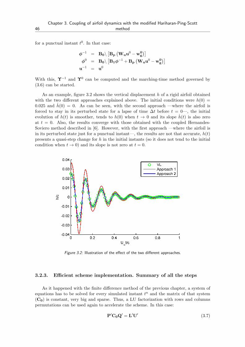
46Chapter 3. Coupling of airfoil dynamics with the modified Hariharan-Ping-Scott
method
for a punctual instant t0. In that case:
φ−1 = B0\[Bp
(Wuu0 −w0
g
)]φ0 = B0\
[B1φ
−1 + Bp
(Wuu0 −w0
g
)]u−1 = u0
With this, Υ−1 and Υ0 can be computed and the marching-time method governed by(3.6) can be started.
As an example, figure 3.2 shows the vertical displacement h of a rigid airfoil obtainedwith the two different approaches explained above. The initial conditions were h(0) =0.025 and h(0) = 0. As can be seen, with the second approach —where the airfoil isforced to stay in its perturbed state for a lapse of time ∆t before t = 0—, the initialevolution of h(t) is smoother, tends to h(0) when t → 0 and its slope h(t) is also zeroat t = 0. Also, the results converge with those obtained with the coupled Hernandes-Soviero method described in [6]. However, with the first approach —where the airfoil isin its perturbed state just for a punctual instant—, the results are not that accurate, h(t)presents a quasi-step change for h in the initial instants (so it does not tend to the initialcondition when t→ 0) and its slope is not zero at t = 0.
Figure 3.2: Illustration of the effect of the two different approaches.
3.2.3. Efficient scheme implementation. Summary of all the steps
As it happened with the finite difference method of the previous chapter, a system ofequations has to be solved for every simulated instant tn and the matrix of that system(C0) is constant, very big and sparse. Thus, a LU factorization with rows and columnspermutations can be used again to accelerate the scheme. In this case:
P′C0Q′ = L′U′ (3.7)

3.2. Description of the coupled Hariharan-Ping-Scott method 47
Here, the prime symbol is used to avoid confusions with the matrixes that took partin the LU decomposition used in the previous chapter for the modified HPS method.Following the same reasoning as the one presented in section 2.2.3, it is possible to definethe permuted vector of unknowns Υn as Υn = Q′Υn and to compute it by solving thetwo triangular systems that appear in the following equation:
Υn = U′\(L′\
(C1Υn−1 + C2Υn−2 + Cgwn
g + CQQnext
))(3.8)
where C1 = P′C1Q′, C2 = P′C2Q′, Cg = P′Cg and CQ = P′CQ.
Once Υn is calculated, the values of un can be extracted from it. Indeed, since un
corresponds to the last 2m rows of Υn and Υn = Q′Υn, un can be obtained by multiplyingthe submatrix formed by the last 2m rows of Q′ (say UΥ) by Υn, i.e.:
un = UΥΥn (3.9)
where: (UΥ
)ij
=(Q′)Nφ+i,j
, i = 1, . . . , 2m, j = 1, . . . , Nφ + 2m
In order to clarify all the ideas before, the method has been summarized in the followingsteps:
Input data:
� Flow conditions: ρ∞, U∞, a∞ and wg(t, x).
� Mesh and time simulation data: xi, yj , c, ∆t and tf .
� Mass, damping and stiffness matrixes (M, C, K), initial conditions (qk(t =0), qk(t = 0)) and external generalized forces (Qextk (t)).
� Shape functions ψk(x) and their derivatives ψ′k(x).
First, compute matrixes A0 and A1 as pointed in section 2.2.2; then, calculate B0,B1, B2 and Bp as shown in section 2.2.1; and finally, construct matrixes C0, C1,C2, Cg and CQ as explained in section 3.2.1.
Perform the LU factorization of C0 with rows and columns permutations (equation(3.7)).
Permute C0, C1, C2, Cg and CQ to obtain C0, C1, C2, Cg and CQ as indicatedjust after equation (3.8). Obtain UΥ as well.
Assume tn = ∆t, calculate Υ−1, Υ0 as pointed in section 3.2.2 and obtain Υ−1 =Q′\Υ−1, Υ0 = Q′\Υ0.
� Evaluate Υn using equation (3.8).
� Extract the generalized coordinates and velocities from Υn through relation(3.9).
� Actualize variables:
Υn−2 ← Υn−1, Υn−1 ← Υn, tn ← tn + ∆t

48Chapter 3. Coupling of airfoil dynamics with the modified Hariharan-Ping-Scott
method
3.3. Results
In order to validate the method described before and to provide simple examples ofpossible applications, it has been tested with three problems: (i) the flutter point calcu-lation of a rigid flat airfoil with two degrees of freedom, (ii) the flutter point calculationof a flexible cantilevered panel and (iii) the response to a sharp-edge gust of a rigid airfoilwith free vertical displacement.
In the first two cases, the flutter Mach number Mf has been calculated as a functionof the upstream sound speed a∞ and the results have been compared with other onesprovided by the coupled Hernandes-Soviero method described in reference [6], gettingexcellent agreement. No other references to compare with have been found in the availableliterature, hence, the results presented here are original or not well-known.
For the third problem, some results have been found in the literature (in reference[20], for example). However, they are not useful for this work because they offer a veryextensive study of the influence of many parameters, and the aim of this section is justto show simple examples that could provide some insight into possible applications of thecoupled HPS method. Thus, the few simple results obtained here will be only validatedwith the coupled vortex-lattice method.
3.3.1. Flutter of a rigid airfoil
Consider a rigid airfoil attached to a fixed point with springs and dampers like theone shown in figure 3.1. The mechanical properties of the system are given by the airfoil’smass ma, the x-coordinate of its gravity centre xg, the x-coordinate of the elastic axis xe,the inertia Ie about that axis, the stiffness constants kh, kα of the linear and torsionalsprings (respectively) and the damping constants ch, cα of the linear and torsional dampers(respectively as well).
If the same degrees of freedom used for the Theodorsen’s problem (as shown in figures2.5 and 3.1) are employed now, the airfoil’s equations of motion read as [9]:[
ma ma(xg − xe)ma(xg − xe) Ie
] [hα
]+
[ch 00 cα
] [hα
]+
[kh 00 kα
] [hα
]=
[Qaeroh
Qaeroα
]It has to be reminded that h and α are measured respect from the equilibrium position.The latter equation provides the mass, damping and stiffness matrixes. On the otherhand, the shape functions associated with the degrees of freedom are:
ψh(x) = −1
ψα(x) = xe − x
Typically, the parameters of the airfoil are described in terms of the following non-dimensional variables:
µ =ma
ρ∞πb2, xα =
xg − xeb
, a =xe − bb
, r2α =
Iemab2
where b = c/2 is the semi-chord of the airfoil. Also, the natural frequencies that the airfoil

3.3. Results 49
would have if it could only experiment vertical or rotational motion are used:
ωh =
√khma
, ωα =
√kαIe
Once the parameters of the airfoil are fixed, the flutter speed can be obtained just bya trial and error procedure. First, a flow speed U∞ is assumed and the airfoil’s motionis computed. If the oscillations’ amplitude decreases (increases), the airfoil’s motion iscalculated again for a higher (lower) flow speed. This is done until a flow speed thatmakes the amplitude keep constant (i.e., the flutter speed) is found.
The results obtained for an airfoil of parameters µ = 2, xα = 0.4, a = −0.4, r2α = 0.25,
ωh/ωα = 0.6 and no damping are presented in figure 3.3. As can be seen there, theflutter Mach number increases when the upstream sound speed decreases, until the latterreaches a minimum value. From that point, Mf and a∞ both increase. Also, it can beobserved that the results provided by this coupled finite differences method show excellentagreement with the ones provided by the coupled vortex-lattice method described in [6].In addition, the solution obtained by neglecting compressibility effects [6] —which is givenby the equation Mfaf = U incf = const., where U incf is the flutter speed in incompressibleregime— has been also represented to check that the solution obtained by the coupledHPS method tends asymptotically to it when M∞ → 0.
Figure 3.3: Flutter Mach number Mf as a function of the upstream sound speed a∞for a rigid airfoil.
At the same time, the response of the airfoil at M∞ = 0.6 and different upstreamvelocities is shown in figure 3.4. In the case where U∞ is equal to the flutter speed Uf , itcan be seen how the oscillations keep their amplitude constant after an initial perturbationtakes the airfoil away from its equilibrium position (h = 0, α = 0). In the cases whereU∞ is greater or lower than the flutter speed, the amplitude of the oscillations decrease orincrease, respectively.

50Chapter 3. Coupling of airfoil dynamics with the modified Hariharan-Ping-Scott
method
Figure 3.4: Evolution of the degrees of freedom along the time for U∞ values that arelower, equal and greater than the flutter speed Uf .

3.3. Results 51
3.3.2. Flutter of a cantilevered flexible plate
Now consider a cantilevered flexible flat plate, like the one shown in figure 3.5, whosedimensions are L×H. Let the incident flow come in the direction given by L and H →∞in order to simulate a two-dimensional problem.
U∞
L
Hx
y
z
Figure 3.5: Scheme of a cantilevered flexible plate submitted to an incident flow.
The equation that governs the displacements of the mean line zp(t, x) of the plate is[8]:
σ∂2zp∂t2
+D∂4zp∂x4
= ∆p (3.10)
where σ is the superficial mass density, D is the flexural rigidity and ∆p is the pressuredifference between the lower and the upper parts of the plate. At the same time, D isgiven by:
D =Eh3
p
12(1− ν2)
where E is the Young’s modulus, hp the plate thickness and ν the Poisson’s coefficient.
At the same time, the displacements of the mean line can be described by a Galerkindecomposition:
zp(t, x) =
m∑i=1
qi(t)ψi(x)
where ψ1(x), . . . , ψm(x) are the first m in vacuo vibration modes, and q1(t), . . . , qm(t) arethe corresponding generalized coordinates. These modes are obtained in reference [2] andread as:
ψi(x) = [sin (βiL)− sinh (βiL)] [sin (βix)− sinh (βix)] + . . .
[cos (βiL) + cosh (βiL)] [cos (βix)− cosh (βix)] (3.11)
where β1 < β2 < . . . are the different solutions of:
cos (βiL) cosh (βiL) + 1 = 0
The modes described by (3.11) have as drawback that involve calculations of hyperbolicsines and cosines. Thus, when a few modes are employed and the different values of βi startincreasing, those hyperbolic sines and cosines become very high and introduce numericalerrors. In order to avoid them, these modes can be divided by e2βiL, limiting then their

52Chapter 3. Coupling of airfoil dynamics with the modified Hariharan-Ping-Scott
method
maximum value. For that purpose, define first the following functions:
S(x) =sinx
ex
C(x) =cosx
ex
Sh(x) =sinhx
ex=
1− e−2x
2
Ch(x) =coshx
ex=
1 + e−2x
2
It is very important to define Sh(x) as (1− e−2x)/2 and not as sinhx/ex, so the computernever calculates the term sinhx, which is the one that introduces the numerical errors.The same can be said for Ch(x). Using this functions, some proportional modes ψ∗i (x) canbe defined as:
ψ∗i (x) =ψi(x)
e2βiL= e−βi(L−x) [[S (βiL)− Sh (βiL)] [S (βix)− Sh (βix)] + . . .
[C (βiL) + Ch (βiL)] [C (βix)− Ch (βix)]]
Again, the latter modes present a problem, which is that some of them have bigger valuesthan others, so they have more weight in the simulations and lead newly to numericalerrors. To solve this inconvenient, the following integral can be performed symbolically:
I∗i =1
L
ˆ L
0(ψ∗i )
2dx
which allows to define new proportional modes:
ψi(x) =ψ∗i (x)√I∗i
These modes verify that the integrals of their square powers are all the same:ˆ L
0ψ2i dx =
1
I∗i
ˆ L
0(ψ∗i )
2dx = L
Thus, they can be expected to have similar values and similar weight in the simulation.
Now, let zp be described in terms of the latter modes and their corresponding gener-alized coordinates qi:
zp(t, x) =m∑i=1
ψi(x)qi(t) (3.12)
It can be shown that those modes verify:
d4ψidx4
= β4i ψi (3.13)
ˆ L
0ψiψjdx = 0 (i 6= j) (3.14)
Using expressions (3.12)-(3.14), equation (3.10) provides the following matricial relation: σL. . .
σL
q1
...qm
+
Dβ41L
. . .
Dβ4mL
q1
...qm
=
Qaero1...
Qaerom
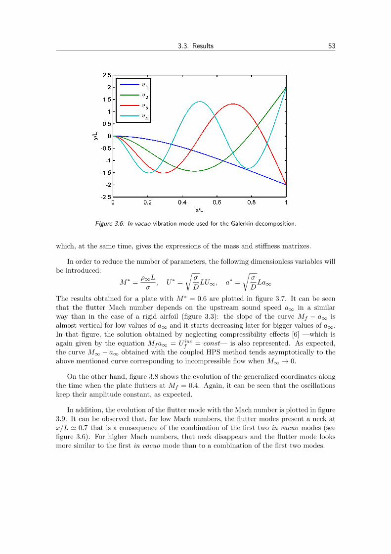
3.3. Results 53
Figure 3.6: In vacuo vibration mode used for the Galerkin decomposition.
which, at the same time, gives the expressions of the mass and stiffness matrixes.
In order to reduce the number of parameters, the following dimensionless variables willbe introduced:
M∗ =ρ∞L
σ, U∗ =
√σ
DLU∞, a∗ =
√σ
DLa∞
The results obtained for a plate with M∗ = 0.6 are plotted in figure 3.7. It can be seenthat the flutter Mach number depends on the upstream sound speed a∞ in a similarway than in the case of a rigid airfoil (figure 3.3): the slope of the curve Mf − a∞ isalmost vertical for low values of a∞ and it starts decreasing later for bigger values of a∞.In that figure, the solution obtained by neglecting compressibility effects [6] —which isagain given by the equation Mfa∞ = U incf = const— is also represented. As expected,the curve M∞ − a∞ obtained with the coupled HPS method tends asymptotically to theabove mentioned curve corresponding to incompressible flow when M∞ → 0.
On the other hand, figure 3.8 shows the evolution of the generalized coordinates alongthe time when the plate flutters at Mf = 0.4. Again, it can be seen that the oscillationskeep their amplitude constant, as expected.
In addition, the evolution of the flutter mode with the Mach number is plotted in figure3.9. It can be observed that, for low Mach numbers, the flutter modes present a neck atx/L ' 0.7 that is a consequence of the combination of the first two in vacuo modes (seefigure 3.6). For higher Mach numbers, that neck disappears and the flutter mode looksmore similar to the first in vacuo mode than to a combination of the first two modes.

54Chapter 3. Coupling of airfoil dynamics with the modified Hariharan-Ping-Scott
method
Figure 3.7: Dependency of the flutter Mach number Mf with the upstream sound speeda∞ for a flexible plate.
Figure 3.8: Evolution of the generalized coordinates along the time when the flexibleairfoil flutters.

3.3. Results 55
Figure 3.9: Flutter mode for different Mach numbers and M∗ = 0.6.

56Chapter 3. Coupling of airfoil dynamics with the modified Hariharan-Ping-Scott
method
Finally, as a way to check the quality of the results, the flutter mode obtained nu-merically for M∗ = 0.74 and incompressible regime is compared in figure 3.10 with theone obtained experimentally by Eloy and others [8]. As can be seen, both modes lookvery similar, only being a slight discrepancy in the size of the neck. This happens dueto two facts: first, the plate used in the experiment is not two-dimensional and, second,the displacements are not really small, so non-linear effects should be taken into accountto get more accuracy. Indeed, a good proof of the non-linearity is that the plate doesnot always have its trailing edge at x = L when it flutters, as supposed in the numericalmethod, because its length has to be approximately constant. Anyway, the results showthat the coupled HPS method seems to be accurate and reliable.
Figure 3.10: Comparison of the flutter mode obtained experimentally (below) and withthe coupled HPS method (above) for incompressible flow.

3.3. Results 57
3.3.3. Response to a vertical sharp-edge gust
Let an airfoil that is flying at constant horizontal speed U∞ enter in a vertical sharp-edge gust of intensity w0 = U∞, as shown in figure 3.11. As a consequence of the gust,the airfoil will experiment extra lift (see Kussner’s problem, section 2.3.3) and will startmoving up. The horizontal speed is assumed to keep being U∞. If rotation and deformationof the airfoil are neglected for simplicity reasons, the movement will be described by theequation:
maη = Qaeroη
where ma and η are the mass and the vertical displacement of the airfoil, respectively.The shape function associated with η is:
ψη(x) = 1
η
U∞
w0 = U∞
Figure 3.11: Airfoil entering in a vertical sharp-edge gust of speed w0 = U∞.
Figure 3.12 shows the airfoil vertical velocity as a function of the elapsed time. Again,the results show good agreement between the coupled finite differences and the coupledvortex-lattice methods. For all Mach numbers, the vertical speed increases at the beginningdue to the extra lift caused by the gust. As that vertical speed becomes bigger, the totalinduced speed over the airfoil decreases, as well as the effective angle of attack (see figure3.13), causing the total lift over the airfoil to diminish. After some time, the verticalspeed is exactly the same as the gust speed, so there are not any induced velocities overthe airfoil, there is not any lift as well and therefore the airfoil stays with that speed. Thatis why η/U∞ → 1 in all the curves.

58Chapter 3. Coupling of airfoil dynamics with the modified Hariharan-Ping-Scott
method
Figure 3.12: Vertical speed of the airfoil η as a function of the elapsed time.
U∞
w0 − η v
αeff
Figure 3.13: Scheme that illustrates the total incident flow velocity (blue) over theairfoil, and the effective angle of attack αeff . The horizontal component is U∞,whereas the vertical one is the difference between the gust speed w0 and the airfoil’svertical velocity η. Hence, when the latter is equal to the first, the effective angle of
attack is null and the lift tends to zero as time increases.
Conclusions and futuredevelopments
In this work, two improvements have been proposed to the Hariharan-Ping-Scottmethod [11] —a finite differences marching-time scheme that calculates the two-dimensionalunsteady linearized potential flow past an airfoil. The first consists in employing a non-uniform mesh to focus more points near the airfoil, which is the origin of the convectedwaves, clearly accelerating the convergence of the solution. The second relies on usinga BDF implicit time integration scheme, making the algorithm much more stable andallowing to take bigger time step sizes.
The scheme modified with those improvements, which has been renamed as modifiedHariharan-Ping-Scott method, is only valid for problems where the airfoil motion is known.Thus, to make it useful for solving aeroelasticity problems where the airfoil motion is justthe unknown, such as flutter, it has been coupled with the airfoil dynamics in a waythat is valid for any airfoil (flexible or rigid, cantilevered or hinged, etc.) that presents alinear equation of motion. This coupling has proved to be accurate and has also providedresults that have not been found in the available literature, such as the flutter of a flexiblecantilevered panel.
Also, the efficiency of the modified Hariharan-Ping-Scott method and the modifiedHernandes-Soviero method’s —a vortex-lattice scheme presented by Hernandes and So-viero [12][13] modified with a truncation algorithm proposed by Colera and Perez-Saborid[6]— have been compared. For short simulations, the modified Hernandes-Soviero methodhas proved to be the fastest one because the number of unknowns (the potential at theairfoil points) is lower. However, for long simulations, the modified Hariharan-Ping-Scottmethod is the fastest one because, despite of the bigger number of unknowns (the potentialat the whole mesh, not only in the airfoil points), it does not have to calculate the influenceof great part of the history before, as it happens in the Hernandes-Soviero method.
The latter conclusion can be extended out of the unsteady aerodynamics field to saythat, in general, finite differences methods can be faster than boundary element methodswhen solving the two-dimensional wave equation in the time domain4. Indeed, since two-dimensional waves have a dissipative nature, a wave that is generated at any point willalways affect to all the space inside its wavefront. Thus, for solving any 2D wave equationin the time domain with a boundary element method —such as the vortex-lattice— it isnecessary to store the whole evolution of the variables at the boundaries —or part of it if
4Of course, boundary elements methods may present other advantages respect finite differences methods,but they are not going to be analysed here.
59

60 Conclusions and future developments
a truncation method is used— and to calculate its influence at every instant, leading tomemory and slowness problems. However, as commented before, finite differences methodsdo not need to store all or great part of the history before and therefore they do not presentthose problems. In return, a bigger number of unknowns has to be handled, but this canbe done in an efficient way by using adequate sparse matrixes.
Both the modified Hariharan-Ping-Scott method and the coupled one with the airfoildynamics (renamed as coupled Hariharan-Ping-Scott method) have proved to give accurateresults in an efficient way. Also, they are useful for any general linear problem, unlikeother methods that are only valid for specific cases like harmonic motion or rigid profile.Thus, they can be an excellent tool for preliminary designs, where the CFD conventionalprograms are too expensive for the required accuracy.
In addition, both methods are very intuitive because they rely on the physics beyondthe fundamental equations of the linearized unsteady potential flow theory and do not leavethe time domain, unlike the classical approach for the theory, which uses many tediousmathematical developments in the frequency domain. Also, they can be implemented withprograms like Matlab, which is accessible to students, has a simple syntax that is easyto understand and also permits an efficient program run. Hence, they can be used as ateaching application.
Some future developments are proposed to improve the commented methods:
The use of higher-order formulas to approximate both the spatial and the timederivatives. This would provide more accuracy, but it must be done with care becauseit could also bring stability problems.
To use an adaptive time step size instead of a fixed one.
To extend the method for supersonic regime.
To extend the methods for a three-dimensional domain. However, it has to beremarked that a boundary element method (vortex-lattice, doublet-lattice or anyother) could be more efficient for that case because the number of unknowns wouldbe much lower and, as well, it would not be necessary to compute all the historybefore since three-dimensional waves are non-dispersive (see figure 3.14).

61
Airfoil Wake
Source at tn
κni
Wavefront of the source
at tn + ∆t′
U∞
2D:
U∞
κnij
Source at tn
Wavefront of the source
at tn + ∆t′
3D:
Figure 3.14: Difference between the two-dimensional and three-dimensional cases indoublet-lattice and vortex-lattice methods. When the flow is two-dimensional, anysource, doublet, vortex or fundamental solution κni born at tn affects to the pointsat and inside its wavefront. Thus, it is necessary to store its value during all thesimulation and to compute its influence at every simulated instant. However, when theflow is three-dimensional, any fundamental solution κnij born at tn affects only to pointssituated just at its wavefront. Thus, when the latter goes out of the wing after a time
∆t′, κnij can be erased and its influence does not have to be calculated any more.


Bibliography
[1] E. Alberdi, J.J. Anza: BDF-α: A Multistep Method with Numerical Damping Control.Universal Journal of Computational Mathematics 1(3): 96-108, 2013.
[2] S.S. Arora: Study of Vibration Characteristics of Cantilever Beams of Different Ma-terials. Thapar University, Patiala, 2012.
[3] R.L. Bisplinghoff, H. Ashley, R.L. Halfman: Aeroelasticity. Dover, 1996.
[4] A. Blazquez, M. Perez-Saborid: Clases de Aeroelasticidad, E.T.S.I. Sevilla, curso2012-2013.
[5] J.B. Bratt: Flow Patterns in the Wake of an Oscillating Aerofoil. Aeronautical Re-search Council Reports and Memoranda, 2011-2012.
[6] M. Colera, M. Perez-Saborid: Calculo numerico del flujo potencial no estacionariosobre perfiles en los regımenes subsonico y supersonico. E.T.S.I. Sevilla, 2015.
[7] D. Eberly: Derivative Approximation by Finite Diferences. Geometric Tools, LLC,2015.
[8] C. Eloy, R. Lagrange, C. Souillez, L. Schouvellier: Aeroelastic instability of can-tilevered flexible plates in uniform flow. Journal of Fluid Mechanichs, Vol 611, pags97.106, 2006.
[9] Y.C. Fung: An Introduction to the Theory of Aeroelasticity. Dover, 2008.
[10] U. Gulcat: Fundamentals of Modern Unsteady Aerodynamics. Springer, 2010.
[11] S.I: Hariharan, Y. Ping, J.R. Scott: Time Domain Numerical Calculations of Un-steady Vortical Flows about a Flat Plate Airfoil. Journal of Computational Physics101, 419-430, 1992.
[12] F. Hernandes, P.A.O. Soviero: Unsteady Aerodynamic Coefficients Obtained by aCompressible Vortex-Lattice Method. Journal of Aircraft, Vol 46, No 4, 2009.
[13] F. Hernandes, P.A.O. Soviero: A Numerical Model for Thin Airfoils in UnsteadyCompressible Arbitrary Motion. J. of the Braz. Soc. of Mech., Sci. & Eng., 2007.
[14] A. Kayran: Kussner’s Function in the Sharp-Edged Gust Problem - A Correction.Journal of Aircraft, Vol 43, No 5, 2006.
[15] J. Katz, A. Plotkin: Low-Speed Aerodynamics. Cambridge University Press, 2001.
63
64 Bibliography
[16] D. Mateescu: Theoretical solutions for unsteady compressible subsonic flows past oscil-lating rigid and flexible airfoils. Mathematics in Engineering, Sciencie and Aerospace,Vol 2 No 1, 2011.
[17] MatLab LU documentation. MathWorks, 2016.
[18] W.J. McGroskey, J. Aircraft, 22(3), 236 (1985).
[19] I.F. Miranda, P.A.O. Soviero: Inditial Response of Thin Wings in a CompressibleSubsonic Flow. 18th International Congress of Mechanical Engineering, November6-11, 2005.
[20] M.J. Patil, D.J. Taylor: Gust Response of Highly Flexible Aircraft. American Instituteof Aeronautics and Astronautics.
[21] T. Theodorsen: General Theory of Aerodynamic Instability and the Mechanism ofFlutter. NACA Tech. Rep. 496, 1935.