Embed Size (px)
Citation preview

UNIVERIDAD POLITÉCNICA DE MADRID
ESCUELA TÉCNICA SUPERIOR DE INGENIEROS DE
TELECOMUNICACIÓN
TRABAJO FIN DE GRADO
Grado en Ingeniería de Tecnologías y Servicios de Telecomunicación
DEVELOPMENT OF A VISUAL OBJECT TRACKING
SYSTEM USING COMPRESSIVE SENSIG FRAMEWORK
FOR MODELLING THE APPEARANCE
DESARROLLO DE UN SISTEMA DE SEGUIMIENTO DE
OBJETOS USANDO LA TEORÍA DE “COMPRESSIVE
SENSING” PARA MODELAR LA APARIENCIA
Ana Mantecón Jené
Julio 2015
TRABAJO FIN DE GRADO

Autor: ANA MANTECÓN JENÉ
Tutor: CARLOS ROBERTO DEL BLANCO ADÁN
Departamento: GRUPO DE TRATAMIENTO DE IMÁGENES
TRIBUNAL
Presidente: LUIS SALGADO ÁLVAREZ DE SOTOMAYOR
Vocal: FRANCISCO MORÁN BURGOS
Secretario: CARLOS ROBERTO DEL BLANCO ADÁN
Suplente: CARLOS CUEVAS RODRÍGUEZ
CALIFICACIÓN:
Madrid, a de 2015.

ABSTRACT
In the following work, we address the commonly known problem of visual object
tracking, which tries to find the trajectory of an object in a video sequence. This task is carried
out by developing a tracking-by-detection method that builds up an effective appearance model
in the compressed domain via compressive sensing theory. The only information about the
sequence that our approach needs to know in advance is the location of the target object in the
first frame.
Visual tracking is a classical field of computer vision that has been addressed for many
years. However, it is still a very challenging task as many variables such as illumination changes,
object occlusion, and the complexity of the background, have to be accounted in order to build
a robust tracking algorithm.
To deal with these challenges, we propose a tracking-by-detection algorithm that trains
an SVM classifier in an online manner to separate the object from the background. We generate
the appearance model with a robust high dimensional feature descriptor that describes the
objects and the surrounding background of the scene. This step is followed by a dimensionality
reduction step that enables to train and use the classifier with a much lower dimension of the
data.
The dimensionality reduction step is based on the compressive sensing theory that
states that a sparse signal can be well-represented and recovered from a small sets of
measurements. The compressive sensing problem is also addressed and described in this work,
and different measurement and recovery techniques are tested to evaluate the resulting
reduced vectors. The purpose is to verify that they are able to keep the essence and information
of the high dimensional vectors.
We also perform a successful update of the object appearance model by using the current
tracker state to extract positive and negative samples, which are used to re-train the classifier.
This way our tracker is able to adapt to the appearance variation of the object.
The proposed tracking algorithm is evaluated with challenging video sequences, and also
compared with other state-of-the-art trackers, proving the success of the performance of our
algorithm.
KEY WORDS
Visual object tracking, compressive sensing, dimensionality reduction, appearance model,
classifiers, DSLQP descriptor, online learning.

RESUMEN
En el presente trabajo se aborda el problema del seguimiento de objetos, cuyo objetivo
es encontrar la trayectoria de un objeto en una secuencia de video. Para ello, se ha desarrollado
un método de seguimiento-por-detección que construye un modelo de apariencia en un
dominio comprimido usando una nueva e innovadora técnica: “compressive sensing”. La única
información necesaria es la situación del objeto a seguir en la primera imagen de la secuencia.
El seguimiento de objetos es una aplicación típica del área de visión artificial con un
desarrollo de bastantes años. Aun así, sigue siendo una tarea desafiante debido a varios
factores: cambios de iluminación, oclusión parcial o total de los objetos y complejidad del fondo
de la escena, los cuales deben ser considerados para conseguir un seguimiento robusto.
Para lidiar lo más eficazmente posible con estos factores, hemos propuesto un algoritmo
de tracking que entrena un clasificador Máquina Vector Soporte (“Support Vector Machine” o
SVM en sus siglas en inglés) en modo online para separar los objetos del fondo de la escena. Con
este fin, hemos generado nuestro modelo de apariencia por medio de un descriptor de
características muy robusto que describe los objetos y el fondo devolviendo un vector de
dimensiones muy altas. Por ello, se ha implementado seguidamente un paso para reducir la
dimensionalidad de dichos vectores y así poder entrenar nuestro clasificador en un dominio
mucho menor, al que denominamos domino comprimido.
La reducción de la dimensionalidad de los vectores de características se basa en la teoría
de “compressive sensing”, que dice que una señal con poca dispersión (pocos componentes
distintos de cero) puede estar bien representada, e incluso puede ser reconstruida, a partir de un
conjunto muy pequeño de muestras. La teoría de “compressive sensing” se ha aplicado
satisfactoriamente en este trabajo y diferentes técnicas de medida y reconstrucción han sido
probadas para evaluar nuestros vectores reducidos, de tal forma que se ha verificado que son
capaces de preservar la información de los vectores originales.
También incluimos una actualización del modelo de apariencia del objeto a seguir,
mediante el re-entrenamiento de nuestro clasificador en cada cuadro de la secuencia con
muestras positivas y negativas, las cuales han sido obtenidas a partir de la posición predicha por
el algoritmo de seguimiento en cada instante temporal.
El algoritmo propuesto ha sido evaluado en distintas secuencias y comparado con otros
algoritmos del estado del arte de seguimiento, para así demostrar el éxito de nuestro método.
PALABRAS CLAVE
Seguimiento de objetos, compressive sensing, reducción de la dimensionalidad, modelo de
apariencia, clasificadores, descriptor DSLQP, aprendizaje en línea.

TABLE OF CONTENTS
1. INTRODUCTION ................................................................................................................. 1
1.1 Motivation .................................................................................................................... 1
1.2 Objectives ................................................................................................................... 2
1.3 Structure ..................................................................................................................... 2
2 STATE OF THE ART ............................................................................................................ 3
2.1 Introduction .................................................................................................................. 3
2.2 Tracking challenges ...................................................................................................... 3
2.3 General object tracking ................................................................................................ 5
2.4 State of the art about trackers ..................................................................................... 6
3 COMPRESSIVE SENSING THEORY .................................................................................. 13
3.1 Introduction ................................................................................................................ 13
3.2 Fundamental concepts of compressive sensing .......................................................... 14
3.2.1 Basis representations .......................................................................................... 14
3.2.2 Sparsity and incoherence .................................................................................... 16
3.3 The compressive sensing problem .............................................................................. 16
3.4 Measurement process ................................................................................................ 18
3.5 Reconstruction process .............................................................................................. 21
3.6 Compressed learning ..................................................................................................22
3.7 Conclusions ................................................................................................................ 23
4 DESCRIPTION OF THE DEVELOPED COMPRESSED SENSING BASED TRACKING
FRAMEWORK .......................................................................................................................... 24
4.1 Introduction ............................................................................................................... 24
4.2 System overview ....................................................................................................... 24
4.2.1 Feature extraction ............................................................................................... 27
5 TRACKING RESULTS ........................................................................................................ 31
5.1 Introduction ................................................................................................................ 31
5.2 Evaluation of the reduced vectors .............................................................................. 31
5.3 Database and metrics ................................................................................................. 32

5.4 Experimental results ................................................................................................... 35
5.4.1 Quantitative comparisons ................................................................................... 39
6 CONCLUSION AND FUTURE WORK ............................................................................... 44
REFERENCES .......................................................................................................................... 46

TABLE OF FIGURES
Figure 1. Background clutter ...................................................................................................... 4
Figure 2. Partial object (face) occlusion ..................................................................................... 4
Figure 3. Illumination changes. (a) and (b) are different frames from the same sequence. ........ 4
Figure 4. General visual object tracking structure ....................................................................... 5
Figure 5. (a) Original signal with pixel values between [0,255]. (b) Wavelet coefficients of the
image. (c) Reconstruction of the image by a small subselection of its wavelet coefficients. ..... 16
Figure 6. Compressive sensing problem. .................................................................................. 17
Figure 7. Compressive sensing process example. ...................................................................... 17
Figure 8. Compressive sensing boundaries for a signal with a sparsity of 98% ..........................20
Figure 9. Compressive sensing measurement process. .............................................................20
Figure 10. The 𝑙1- minimization problem coincides with the sparsest solution ........................22
Figure 11. Training phase at the n-th frame .............................................................................. 25
Figure 12. Tracking phase at the (n+1)-th frame ....................................................................... 25
Figure 13. SVM training ............................................................................................................ 26
Figure 14. Feature extraction implemented. ............................................................................. 27
Figure 15: Local Binary Pattern example: (a) Grey scale neighborhood. (b) Computed intensity
differences. (c) Binary value. .................................................................................................... 28
Figure 16: DSLQP descriptor. .................................................................................................. 28
Figure 17. Histogram concatenation ........................................................................................ 29
Figure 18. Compressive Sensing reconstruction example. ....................................................... 33
Figure 19. (a) Positive sampling region and (b) Negative sampling region. ............................... 36
Figure 20: Average Success Rate graphics. ............................................................................... 37
Figure 21. Challenging frames in Cliffbar sequence .................................................................. 38
Figure 22. Challenging frames in Trellis sequence .................................................................... 39
Figure 23. Challenging frames in Sylv sequence ....................................................................... 39
Figure 24. Challenging frames in Football sequence ................................................................. 39

TABLE OF TABLES
Table I: Summary of the most relevant state-of-the-art trackers. ............................................ 12
Table II: Different DSLQP configurations. ................................................................................ 31
Table III: MSE computed for each feature vector. ..................................................................... 32
Table IV: Database video sequences. ........................................................................................ 34
Table V: Best Success Rate for each video sequence with each matrix evaluated ..................... 37
Table VI: Best parameters and results for Cliffbar, Trellis, Sylv and Jumping video sequences. 38
Table VII: Table with the Success Rate (%) results of 12-state-of-the-art trackers and our
developed. The best results are shown in red, blue and green fonts respectively. .................... 41
Table VIII: Table with the Center Error Rate (%) results of 12-state-of-the-art trackers and our
developed tracker. The best results are shown in red, blue and green fonts respectively. ....... 42
Table IX: Table with the Success Rate (%) results in a selection of videos of the considered
database. The best results are shown in red, blue and green fonts respectively. ...................... 43

1
1. INTRODUCTION
1.1 MOTIVATION
A classical problem within the field of computer vision is visual object tracking, whose
main goal is to generate trajectories of objects of interest by means of the analysis of video
sequences.
In the past decades, object tracking algorithms have become very popular due to the proliferation of high-powered computers, the availability of high quality and inexpensive video cameras, and the increasing need for automated video analysis.
Object tracking is being used nowadays in many different fields such as:
Motion-based recognition: human identification based on the way each person
moves, automatic object detection, etc.
Automated surveillance: monitoring a scene to detect suspicious activities or
unlikely events.
Human-computer interaction: gesture recognition, face recognition, etc.
Traffic monitoring: acquisition of real time traffic statistics.
Vehicle navigation: video based path planning and obstacle avoidance.
All these fields require a robust tracking algorithm that is stable and computationally
efficient.
One fundamental part in object tracking is the modeling of the object appearance (and
sometimes the surrounding background) that usually depends on the application domain of
each tracker. A common approach is to generate a description of the object appearance in the
form of a feature vector that is invariant, or at least robust, to the tracking challenges. However,
robust and accurate models imply extremely long feature vectors that are difficult to manage
and process, especially under real-time restrictions, or practical memory limitations. In addition,
their processing is affected by the so-called “curse of dimensionality” that can drastically reduce
the tracking performance.
Compressive Sensing is a revolutionary signal processing technique that can be used to
greatly reduce the dimensionality of the long feature vectors that encode the object
appearance, but preserving almost all the information. Compressive Sensing states that signals
that have certain characteristics can be sampled and recovered with much fewer measurements
than using the Nyquist-Shannon criterion. Because of this fact, it is becoming very popular in
many machine learning problems to transform the data domain to some other appropriate
measurement domain.

2
1.2 OBJECTIVES
The objective of this work is to develop a new appearance model framework for visual
object tracking based on Compressive Sensing. This will allow to use highly accurate and robust
appearance models via a dimensionality reduction step, which would be impossible to apply in
another way for tracking purposes due to memory restrictions and/or the curse of
dimensionality phenomenon.
Different measurements and recovery techniques related to the Compressive Sensing
theory will be tested to evaluate the resulting reduced feature vectors, which will be delivered
to a Support Vector Machine (SVM) classifier to distinguish in each frame in which location the
target object is. This SVM will be trained in an online fashion way to adapt continuously to the
temporal variations of the target object, offering a long, stable, and robust tracking in
challenging situations.
1.3 STRUCTURE
This document is organized as follows. In Chapter 2, a review of how the tracking problem
has been addressed during the past years is elaborated, together with the description of the
most relevant state-of-the-art tracking algorithms. In Chapter 3, an introduction to the
compressive sensing theory is presented. The details of our developed algorithm are described
in Chapter 4, where we propose an efficient tracking algorithm with an appearance model based
on the compressive sensing theory. The results of numerous experiments and performance
evaluations are presented in Chapter 5. We conclude this document in Chapter 6, where the
conclusions obtained during the development of this work are stated, along with the potential
future work that could improve the performance of our tracker.

3
2 STATE OF THE ART
2.1 INTRODUCTION
Tracking can be defined as the problem of estimating the trajectory of an object over time
as it moves around the scene by locating its position in every frame of the video, starting from
the bounding box given in the first frame. Trackers may also provide the complete region of the
image that is occupied by the object at every frame.
Trackers have to deal with objects and backgrounds that can change over time. A key task
of a visual tracking algorithm is to describe the appearance of the objects. In most tracking
algorithms, it is assumed that the object motion has no abrupt changes. Many of them also use
a priori information, such as the initial position and size of the target objects, to simplify the
problem.
In the literature, there has been some success in building trackers for specific object
categories, such as faces [1], humans [2], and mice [3]. However, tracking generic objects has
remained challenging because an object can drastically change its appearance over time.
Nowadays, there is no single approach that can successfully handle all scenarios. The state of
the art is still far from achieving results comparable to the human performance.
In the next sections, different perspectives of the tracking task are addressed. Firstly, the
main challenges that the tracking algorithms have to face are presented. Secondly, the general
structure of how the trackers usually handle the tracking problem is described, and also the main
approaches that have been used are introduced. And finally, the most relevant state-of-the-art
trackers will be presented.
2.2 TRACKING CHALLENGES
Visual tracking is a very challenging task as many variables have to be accounted for in
order to build a robust algorithm. The main problems arise from:
Loss of information caused by projection of the 3D world on a 2D image.
Noise in images.
Complex object motion.
Partial and full object occlusions.
Complex object shapes.
Background clutter (complex background).
The deformable and/or articulable nature of certain objects
Illumination changes of the object and the scene.
Real-time processing requirements.

4
Abrupt camera or object motion.
In the next images, we can see some examples of background clutter, partial object occlusion, and illumination changes.
Figure 1. Background clutter
Figure 2. Partial object (face) occlusion
Figure 3. Illumination changes. (a) and (b) are different frames from the same sequence.
The object appearance variations can also be classified as intrinsic and extrinsic variations.
Considering pose and shape object variations, as intrinsic; and illumination changes, camera
motion and perspective, and object occlusion, as extrinsic.

5
2.3 GENERAL OBJECT TRACKING
A typical tracking system can be decomposed into five components:
Target Region.
Appearance Model: Object Feature Description.
Motion model.
Object detection and tracking.
Model update.
Figure 4. General visual object tracking structure
The target region module defines the region that contains the object to be tracked. The
most common strategy is to use a rectangle (bounding box), an ellipse, or a circle. Alternatively,
points can be used, which are appropriate for tracking small objects. Silhouette can be also used
to define the target boundaries, which is effective for specific trackers, such as those that track
pedestrians.
The appearance model of the object of interest is initially built from the target region,
and later is updated along the time by the model update module. It represents the objects
according to its appearance properties: colour, texture, and pixel intensities. The model is
usually a feature vector that is obtained from a feature descriptor technique that synthesizes the
appearance or shape of an image region. In tracking many different feature descriptors have
been used. Some of them are simple, but computationally efficient, such as the Haar-like
features [17][18]. Others are more complex descriptors, such as SIFT (Scale Invariant Feature
Transform) [19], and SURF (Speeded Up Robust Features) [20] descriptors.
The motion model predicts the location of the object by defining also a searching
strategy used to find the most likely regions where the object in the current frame can be. Most
trackers assume that the target is close to its location in the previous frame. However, if the
motion of the target is fast, the target can be lost. More sophisticated strategies define other
searching mechanisms, such as a uniform based sampling search from previous target location
[21], a probabilistic Gaussian search also centered on the previous target location, as in IVT [22],
or motion prediction based on a linear model to reduce the search space [23].
Input
Video
Target
Region
Appearance
model Motion
model
Object
detection and
tracking
Model update Target
Location

6
The object detection and tracking module makes the decision of the new location of the
target by fusing information from previous modules (object appearance and motion), and other
prior information. This way, it generates the trajectory of an object over time by locating its
position in every frame of the video. The tasks of detection and tracking can be performed
separately or jointly. In the first case, possible object regions in every frame are obtained by an
object detection algorithm, and then the tracker estimates the best detection correspondences
across frames. In the second case, the object region and its correspondences are estimated
jointly by means of template matching techniques and snakes.
A common approach to object detection is to use the information obtained from just one
frame of the video. However, there are other methods that use the temporal information from
a set of frames to build a more robust tracker reducing false detections.
The last module, the model update, accounts for appearance variations computing an
update of the appearance model.
2.4 STATE OF THE ART ABOUT TRACKERS
In the literature, many visual object trackers have been proposed. However, not all of them
provide a robust performance in challenging sequences. In this section, a review of the most
relevant works is presented. In section 5, we will make a comparison of our proposed method
with these other methods in terms of their ability to track objects and handle both intrinsic and
extrinsic appearance object variations.
It is of prime importance to build an effective appearance model in order to build a
successfully tracking algorithm. Based on the appearance models, tracking algorithms can be
categorized as either generative [5][22][41][42][43][46], or discriminative [13][18][45][48].
Generative tracking algorithms learn a model to represent the target object, which is
used to find the image regions which are most similar to the target model, considering some
minimal reconstruction error. For example, the IVT method [22] incrementally learns a low-
dimensional subspace representation of the target to adapt to appearance changes, and the 𝑙1-
tracker [5] represents the objects model with a sparse combination of target and trivial
templates.
Discriminative algorithms treat the tracking problem as a detection task. This approach,
also known as tracking-by-detection, has become very popular recently due to the great
progress of object detection.
These algorithms aim to difference the target from the background. The classifier is
trained with object features from an associated object class, and with background features
associated with a different class. This way, the classifier is trained to distinguish between the
7
target object and the background, by finding a decision boundary that separates one from the
other in the defined feature space. The classifier estimates the object location on a new frame
by searching for the maximum classification score in a local region around the location of the
target on the previous frame. Given an estimated object location, positive and negative samples
are chosen to update the appearance model. Commonly this is done by taking the current
tracker location as one positive training example, and sampling the distant neighborhood to get
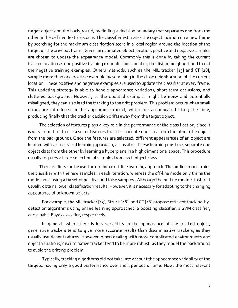
the negative training examples. Others methods, such as the MIL tracker [13] and CT [18],
sample more than one positive example by searching in the close neighborhood of the current
location. These positive and negative examples are used to update the classifier at every frame.
This updating strategy is able to handle appearance variations, short-term occlusions, and
cluttered background. However, as the updated examples might be noisy and potentially
misaligned, they can also lead the tracking to the drift problem. This problem occurs when small
errors are introduced in the appearance model, which are accumulated along the time,
producing finally that the tracker decision drifts away from the target object.
The selection of features plays a key role in the performance of the classification, since it
is very important to use a set of features that discriminate one class from the other (the object
from the background). Once the features are selected, different appearances of an object are
learned with a supervised learning approach, a classifier. These learning methods separate one
object class from the other by learning a hyperplane in a high dimensional space. This procedure
usually requires a large collection of samples from each object class.
The classifiers can be used an on-line or off-line learning approach. The on-line mode trains
the classifier with the new samples in each iteration, whereas the off-line mode only trains the
model once using a fix set of positive and false samples. Although the on-line mode is faster, it
usually obtains lower classification results. However, it is necessary for adapting to the changing
appearance of unknown objects.
For example, the MIL tracker [13], Struck [48], and CT [18] propose efficient tracking-by-
detection algorithms using online learning approaches: a boosting classifier, a SVM classifier,
and a naive Bayes classifier, respectively.
In general, when there is less variability in the appearance of the tracked object,
generative trackers tend to give more accurate results than discriminative trackers, as they
usually use richer features. However, when dealing with more complicated environments and
object variations, discriminative tracker tend to be more robust, as they model the background
to avoid the drifting problem.
Typically, tracking algorithms did not take into account the appearance variability of the
targets, having only a good performance over short periods of time. Now, the most relevant

8
state-of-the-art trackers manage adapting appearance models to address this limitation. The
next list presents a selection of the most representative ones:
Incremental learning visual tracker (IVT) [22]. The IVT is a generative tracking method
that learns the dynamic appearance of the target via an incremental principal component
analysis (PCA) technique. The appearance of the target is represented by a low-
dimensional subspace that provides a compact notion of the object to be tracked,
instead of treating the target as an independent set of pixels. The incremental PCA
algorithm continually updates the subspace model to account for the appearance
changes of the target during the tracking.
This method, proposed by Ross et al, is effective to handle appearance changes
caused by illumination and pose variation. However, it is not robust to some challenging
factors such as partial occlusion and background clutter, mainly due to the fact that it
uses new observations to update the appearance model without previously detecting
outliers.
Fragments-based visual tracker (Frag) [41]. In the Frag tracker, the target object is
represented by multiple image fragments or patches. The location of the object in the
first frame is known, and then multiple rectangular regions (fragments) are selected at
each new frame close to the previous object neighbourhood. For every fragment, an
integral image histogram is extracted, and a voting map is created representing the
comparison of each candidate histogram with the corresponding image patch
histogram. Finally they minimize an error function in order to combine all the vote maps
of the multiple fragments. The position with the minimum error value is selected as the
new target position.
The frag tracker is a generative tracker that is able to handle partial occlusions and
pose changes due to the multiple votes, and also takes into account the spatial
distribution of the pixel intensities. However, patch-based model is not updated, and
therefore this tracker is sensitive to large appearance changes.
Multiple instance learning tracker (MIL) [13]. The MIL tracker is a discriminative tracking-
by-detection algorithm that uses the previous tracker position to extract positive and
negative samples from the current frame. Their image representation consists of a set of
Haar-like features that are computed for each image patch (sample). The appearance
model is updated by using a new online boosting classifier.
This tracker presents a novel approach for tracking, since until then there was no
tracker in the literature that was based on multiple instance learning. It is able to handle
appearance changes due to their continuous updating of the model. However, it is shown

9
that the tracker decision is drifted into the background of the scene when there are
severe illumination changes.
Visual tracking decomposition tracker (VTD) [42] . The VTD tracker decomposes the
tracking problem into several basic motion and observation models, and allows them to
interact. The appearance model is represented by multiple basic observation models that
are constructed by a sparse principal component analysis (SPCA). Each observation
model covers a specific appearance of the object, such as its pixel intensities, edges, or
saturation. The motion model is also represented by the combination of two basic
motion models, one represents smooth motions, and the other one represents abrupt
motions. Then, they design multiple basic trackers by associating the basic observation
models and the basic motion models, so that each specific tracker takes charge of a
certain change in the object. Finally, all trackers are combined interactively.
This tracker is shown to efficiently address the tracking of an object whose motion
and appearance change drastically.
Least Soft-threshold Squares Tracking (LSST) [47]. The LSST tracker proposes a
generative tracking approach based on the Least Soft-threshold Squares (LSS) method,
and build a dictionary (appearance model) using PCA basis vectors. They calculate a LSS
distance to measure the difference between an observation sample and their learned
dictionary. They also add an update scheme to account for appearance changes. They
show that the LSS distance provides good performances when handling outliers (e.g.
dealing with partial occlusion).
Structured output tracking with kernels (Struck) [21]. The Struck tracker handles the
tracking problem with a discriminative approach that learns online a kernelized
structured support vector machine (SVM) to provide an adaptive tracking. To describe
the target object, they use Haar-like features that the classifier learns to build up and
continuously update the appearance model. This tracker takes advantage of the well-
known SVM classifier, which provides a lot of benefits in terms of robustness to noise.
Real Time Compressive tracking (CT) [18]. This tracking algorithm is a tracking-by-
detection algorithm that builds a discriminative appearance model from features
extracted in the compressed domain, and tries to separate the target from its
surrounding background via a simple Bayes online classifier. Positive and negative
samples are extracted at each new frame to update the model.
To build their appearance model, each sample is described as simple generalized
Haar-like features, and compressive sensing is used as a dimensionality reduction
technique to obtain features in a much lower dimension, leading to an efficient real-time
tracker. However, the simplicity of the Haar-like features makes this method not very
robust to heavy occlusion, or abrupt appearance object changes. Other representations

10
such as local binary patterns have been shown to be more effective in handling this kind
of variations.
𝐿1 - tracker (L1) [5]. The 𝐿1 - tracker is a generative algorithm that assumes that the
tracked object can be well represented by a sparse linear combination of object
templates, and trivial templates. Object templates are used to describe the object class
to be tracked, and the trivial templates are used to handle noise and occlusion. Each
trivial template has only one nonzero element, representing a specific feature. A good
target candidate should involve fewer trivial templates. A candidate sample is sparsely
represented by both target and trivial templates, and its corresponding likelihood is
determined by the reconstruction error obtained via 𝑙1- minimization with respect to
previously known target templates. Finally, the tracking result is chosen as the target
template with the minimal reconstruction error.
This innovative tracking method, developed by Mei et al. has been demonstrated
to be very robust against partial occlusions. However, there are several issues to be
addressed. First, the reconstruction error obtained via 𝑙1- minimization requires high
computational cost. Secondly, the reconstruction error of templates, representing an
occluded target and the background, can be both small, and therefore the final selection
of the target template, as de the minimal reconstruction error, may be wrong and cause
the tracker to fail.
The 𝐿1- tracker is the first tracking approach to deal with the representation of an
object as a sparse representation. Due to its high success, it has been used as a reference
for many other trackers.
Multi-task sparse learning tracker (MTT) [43]. Zhang et al. developed the MTT tracker
inspired by the success of the 𝐿1- tracker. They proposed a multi-task sparse learning
approach for visual tracking in a particle filter framework. They model the particles as a
linear combination of dictionary templates that are updated dynamically. The next
target state is selected to be the particle that has the highest similarity with a dictionary
of target templates. They also exploit the similarities among particles to find a joint
representation, which is an improvement from the 𝐿1- tracker that handled particles
independently. They prove that this approach is able to deal with partial occlusion more
accurately. Moreover, learning the particles representation jointly makes their approach
significantly faster than the 𝐿1- tracker.
Online Robust Non-negative Dictionary Learning for Visual Tracking (ONND) [44]. Based
on the 𝐿1 - tracker, Wang et al. proposed an online robust non-negative dictionary
learning algorithm for updating the target templates, so that each learned template can
capture a distinctive aspect of the tracked object. Their approach combines the past
information with the current tracking result. The object representation is formulated

11
using the Huber loss function. This way they do not need to use trivial templates, leading
to a significant reduction of the computational cost. Moreover, they are able to
automatically detect and reject occlusion and clutter background.
Visual tracking via adaptive structural local sparse appearance model (ASLA) [46]. As
previously described, sparse representations have been exploited by previous trackers
[5][43][44] to find the best candidate by looking at the minimal reconstruction error.
However, most of these trackers only consider the holistic representation of the objects
to discriminate between the target and the background, which can lead to failure when
there are similar objects, or occlusions in the scene.
The ASLA tracker develops a tracking method based on a structural local sparse
appearance model that exploits both partial and global spatial information. The
algorithm samples overlapped local image patches near the target region, and obtains a
similarity measure of each sample with the previously obtained target region. It also has
an adaptive update strategy to account for appearance changes of the target. This
tracker is able to handle partial occlusion quite effectively.
Sparsity-based collaborative tracker (SCM) [45]. The SCM tracker is a hybrid method that
combines both generative and discriminative approaches. The representation scheme
for object tracking consists of holistic intensity templates and local histograms. They
build a collaborative model that integrates a sparse discriminative classifier based on the
holistic templates, and a generative model using local representations that consider the
spatial information, and add an occlusion handling scheme. The update of the
appearance model considers both the latest observations and the current one, so as to
deal with the appearance changes.
This tracker effectively deals with cluttered background due to its discriminative
approach, and with heavy occlusion due their developed occlusion handling module.
In Table I, a summary of the state-of-the-art trackers previously described is presented.

12
Table I: Summary of the most relevant state-of-the-art trackers.
Trac
kers
Obj
ect r
epre
sent
atio
n A
dapt
ive
appe
aran
ce m
odel
App
roac
h C
lass
ifier
IVT
[22]
hol
istic
imag
e in
tens
ity
incr
emen
tal
prin
cipa
l com
pone
nt a
naly
sis
gen
erat
ive
-
Frag
[42]
loca
l int
ensi
ty h
isto
gram
– g
ener
ativ
e -
MIL
[13]
Haa
r-lik
e fe
atur
eson
line
mul
tiple
inst
ance
lear
ning
dis
crim
inat
ive
boos
ting
VTD
[43]
hue
, sat
urat
ion,
inte
nsity
and
edge
tem
plat
e s
pars
e pr
inci
pal c
ompo
nent
ana
lysi
s g
ener
ativ
e-
LSST
[48]
holis
tic im
age
inte
nsity
prin
cipa
l com
pone
nt a
naly
sis
gene
rativ
e-
Stru
ck [4
9] H
aar-
like
feat
ures
- d
iscr
imin
ativ
est
ruct
ured
SVM
CT [1
8] H
aar-
like
feat
ures
- d
iscr
imin
ativ
ena
ive
Baye
s
L1T
[5]
hol
istic
imag
e in
tens
itysp
arse
repr
esen
tatio
n g
ener
ativ
e -
MTT
[44]
hol
istic
imag
e in
tens
itym
ulti-
task
spa
rse
lear
ning
gen
erat
ive
-
ON
ND
[45]
holit
ic im
age
inte
nsity
sp
arse
repr
esen
tatio
nge
nera
tive
-
ASLA
[47]
loca
l im
age
patc
hes
spa
rse
repr
esen
tatio
n g
ener
ativ
e -
SCM
[46]
hol
istic
imag
e in
tens
ity a
nd lo
cal
hist
ogra
ms
spar
se re
pres
enta
tion
hyb
ridSD
C (S
pars
ity-b
ased
disc
rimin
aive
cla
ssifi
er)

13
3 COMPRESSIVE SENSING THEORY
3.1 INTRODUCTION
Compressive sensing (CS) has attracted considerable attention in the areas of applied
mathematics, computer science, and electrical engineering by suggesting that it is possible to
surpass the traditional limits of sampling theory, the Shannon-Nyquist sampling theorem.
Shannon-Nyquist sampling theory states that signals (images, videos, and other data) can
be exactly recovered from a set of uniformly spaced samples taken at the so-called Nyquist rate
of twice the highest frequency of the signal of interest.
Digitalization has enabled the growth of sensing systems that are now able to generate a
very large amount of data. Unfortunately, in many applications the number of samples that need
to be taken following the Nyquist rate is very high, and we end up with far too many samples
that are very difficult to manage and process, especially under real-time restrictions or practical
memory limitations.
To cope with the logistical and computational challenges involved in dealing with very
high-dimensional amount of data, compression is usually used. Compression techniques try to
find a mathematical transformation (usually a unitary transformation) that provides a sparse or
compressible representation of a signal of interest, as both sparse and compressible signals can
be well represented by their largest coefficients. More specifically, the meanings of sparse and
compressible in this context are:
Sparse representation: a signal of length 𝑁 that can be represented with 𝐾 << 𝑁
nonzero coefficients.
Compressible representation: a signal of length 𝑁 that is well approximated by a signal
with only 𝐾 nonzero coefficients.
Compressive Sensing is a new theory that grew out of the work of Candès, Romberg, Tao,
and Donoho, which states that a finite-dimensional signal having a sparse representation in a
basis 𝛹 can be recovered from a small set of measurements using a measurement matrix Φ.
Both the measurement matrix and the basis matrix need to be as much incoherent as possible.
Sparsity, incoherence, and basis representations are the fundamental concepts of CS.
In the following sections of this chapter, a brief introduction to the compressive sensing
theory is presented.

14
3.2 FUNDAMENTAL CONCEPTS OF COMPRESSIVE SENSING
3.2.1 Basis representations
Signals can be represented with a basis, called a basis representation of a signal. By
definition it means that the signal can be represented by a fixed set of basis signals (vectors),
each of them with a coefficient associated.
A set of vectors {𝜓𝛾}𝛾=1𝑁
is called a basis for ℝ𝑁, if the vectors are linearly independent and
span all ℝ𝑁. For any x ∈ ℝ𝑁, there exists a unique set of coefficients 𝛼(𝛾) such that:
𝑥(𝑡) = ∑𝛼(𝛾)𝜓𝛾(𝑡)
𝑛
𝛾=1
It is possible to represent different signals with the same basis by changing the coefficients
associated with each basis signal.
A basis representation of a signal can be considered as a way of discretizing it, so as to
make it more manageable to work with. Moreover, it is a linear transformation that makes it
possible to reconstruct the original signal exactly, i.e. it is an invertible transformation.
Basis representations are used very often, for example, when signals are represented in
the Fourier or DCT domain:
𝑥(𝑡) = ∑𝛼(𝑘)𝑒𝑗2𝜋𝑘𝑡
𝑘𝜖ℤ
, 𝑤ℎ𝑒𝑟𝑒 𝜓𝛾(𝑡) = 𝑒𝑗2𝜋𝑘𝑡
A special case of a basis is an orthonormal basis, also known as orthobasis, which is defined
as a set of signals {𝜓𝛾}𝛾=1𝑁
in the space ℝ𝑁 that satisfy the following criteria:
They are orthogonal:
⟨𝜓𝛾, 𝜓𝛾′⟩ = {1 𝛾 = 𝛾′ 0 𝛾 ≠ 𝛾′
where ⟨𝑥, 𝑦⟩ is the dot product.
They have unit norm |𝜓𝛾| = 1, where |x| is the norm of x.
There is no 𝑥 𝜖 ℝ𝑁, 𝑥 ≠ 0, such that ⟨𝜓𝛾, 𝑥⟩ = 0.
In matrix notation, a basis can be represented as a 𝑁𝑥𝑁 matrix 𝛹, whose columns are given
by the basis signals 𝜓𝛾. The orthonormality of a basis means that 𝛹 is orthogonal (its column
vectors or row vectors are an orthonormal set of vectors), which implies that 𝛹𝑇𝛹 = 𝐼, being 𝐼
the 𝑁𝑥𝑁 identity matrix.
(1)
(2)
(3)

15
Orthobasis allow every signal to be decomposed as a linear combination of elements, and
gives a simple way of calculating the coefficients by computing the inner product between the
signal and each basis signal by means of the dot product:
𝛼𝛾 = ⟨𝑥(𝑡) , 𝜓𝛾(𝑡)⟩
To sum up, if {𝜓𝛾}𝛾𝜖 𝛤 is an orthobasis for a generic vector space 𝐻, then every 𝑥 𝜖 𝐻 can
be represented with the following reproducing formula:
𝑥(𝑡) = ∑⟨𝑥(𝑡), 𝜓𝛾(𝑡)⟩𝜓𝛾(𝑡)
𝛾𝜖 𝛤
An important property of having a basis representation of a signal is that it can be
represented in a more compact way as a matrix multiplication. For that, two linear operators are
associated to every orthonormal basis: the synthesis operator and the analysis operator.
Synthesis operator 𝜳. This operator takes a sequence of coefficients and builds up a
signal with them.
𝑥 = 𝛹𝛼
Where 𝛹 is a 𝑁𝑥𝑁 matrix whose columns are given by the basis signals 𝜓𝛾, and 𝛼 is the
length-𝑛 vector of coefficients 𝛼𝛾.
Analysis operator 𝜳𝑻 . This operator maps the signal to a sequence of expansion
coefficients.
𝛼 = 𝛹 𝑇𝑥
It is very important to know that the Parseval theorem is perfectly preserved when a signal
is represented by a complete orthobasis. The Parseval theorem states that if 𝑥(𝑡) is a
continuous-time signal, and 𝛼𝛾 = ⟨𝑥(𝑡) , 𝜓𝛾(𝑡)⟩ are its basis coefficients, then
||𝑥(𝑡)||2= ∫ |𝑥(𝑡)|2 𝑑𝑡 = ∑ |𝛼(𝛾)|2 = ||𝛼||2
𝛾𝜖 𝛤
This means that the energy between the original signal and its coefficients is preserved.
Consequently, the inner product is also preserved. A consequence of the Parseval theorem is
that any space of signals with an orthobasis can be discretized. Also, the energy preservation
essentially means that it preserves all the distance and geometrical relationships of the original
signal in its transformed coefficients.
To sum up, every continuous signal, for which we can find an orthobasis to be represented
with, can be processed by manipulating discrete sequences of numbers (the coefficients).
(4)
(5)
(6)
(7)
(8)
16
3.2.2 Sparsity and incoherence
A signal 𝑥 is 𝐾-sparse if it is composed only by 𝐾 non-zero coefficients:
||𝑥||0 ≤ 𝐾
where ||𝑥||0 is the 𝑙0norm which gives the number of non-zero terms in the vector 𝑥.
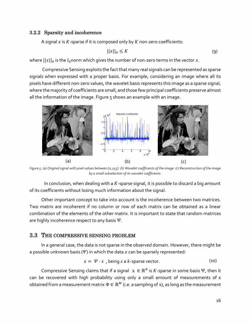
Compressive Sensing exploits the fact that many real signals can be represented as sparse
signals when expressed with a proper basis. For example, considering an image where all its
pixels have different non-zero values, the wavelet basis represents this image as a sparse signal,
where the majority of coefficients are small, and those few principal coefficients preserve almost
all the information of the image. Figure 5 shows an example with an image.
Figure 5. (a) Original signal with pixel values between [0,255]. (b) Wavelet coefficients of the image. (c) Reconstruction of the image
by a small subselection of its wavelet coefficients.
In conclusion, when dealing with a 𝐾-sparse signal, it is possible to discard a big amount
of its coefficients without losing much information about the signal.
Other important concept to take into account is the incoherence between two matrices.
Two matrix are incoherent if no column or row of each matrix can be obtained as a linear
combination of the elements of the other matrix. It is important to state that random matrices
are highly incoherence respect to any basis Ψ.
3.3 THE COMPRESSIVE SENSING PROBLEM
In a general case, the data is not sparse in the observed domain. However, there might be
a possible unknown basis (𝛹) in which the data 𝑥 can be sparsely represented:
𝑥 = 𝛹 · 𝑠 , being 𝑠 a 𝑘-sparse vector.
Compressive Sensing claims that if a signal x ∈ ℝ𝑁 is 𝐾-sparse in some basis Ψ, then it
can be recovered with high probability using only a small amount of measurements of x
obtained from a measurement matrix Φ ∈ ℝ𝑀 (i.e. a sampling of x), as long as the measurement
(a) (c) (b)
(9)
(10)

17
matrix Φ is incoherent with the basis matrix Ψ, and satisfies the Restricted Isometry Property
(RIP), which is stated in the next sub-section. Mathematically:
𝑦 = Φ x = Φ Ψ s = θ s
where 𝑦 is the sampled/measured vector and θ = Φ Ψ is a 𝑀𝑥𝑁 matrix. Notice that the
dimensions of 𝑦 are less than 𝑥 (see Figure 6).
Figure 6. Compressive sensing problem.
The problem of CS can be divided into:
a) Measurement process. Design of a 𝑀 ×𝑁 measurement matrix Φ that ensures that the
information of a k-sparse signal is nearly preserved by the dimensionality reduction
process from x ∈ ℝ𝑁 to y ∈ ℝ𝑀.
b) Reconstruction process. Finding a reconstruction algorithm to recover 𝑥 from only 𝑀 ≪
𝑁 measurements by solving an optimization problem.
Figure 7. Compressive sensing process example.
(11)

18
These both processes, which are intuitively represented at Figure 7, will be explained
further in the following sections.
3.4 MEASUREMENT PROCESS
The measurement process consists on projecting the original signal into a few set of
measurements by means of a measurement matrix Φ. This can be seen as a subsampling of the
signal, in this case a discrete vector. In this section, the compressive sensing measurement
process is reviewed together with an essential property that needs to be fulfilled in order to be
able to successfully represent the high-dimensional signals in the lower dimension. Moreover,
four measurement matrices are presented that satisfy this property, and therefore are
commonly used in CS.
The measurement matrix Φ must allow the reconstruction of the 𝑁 dimensional
signal x ∈ ℝ𝑁 from the vector of measurements y ∈ ℝ𝑀 being 𝑀 ≪ 𝑁.
In general, the position of the 𝐾 non-zero entries of the sparse signal is not known and
variable. On the other hand, the measurement matrix should be fixed in advance for all ℝ𝑁, i.e.
it does not depend on the signal information structure.
The measurement matrix should preserve the information and geometrical relations
between the original vectors and the reduced ones. For this purpose, a sufficient condition for
𝐾-sparse signals is that Φ satisfies the Restricted Isometry Property (RIP).
The Restricted Isometry Property (RIP) was introduced in [29] by Candès and Tao, and
states that a matrix Φ satisfies the RIP for every 𝐾 -sparse vector 𝑥 if there exists a 𝛿𝑘 ∈
(0,1) such that
(1 − 𝛿𝑘)||𝑥||22 ≤ ||Φx||
2
2≤ (1 + 𝛿𝑘)||𝑥||2
2
where ||𝑥||2 is the Euclidean norm of 𝑥.
If a matrix Φ satisfies the RIP, then Φ approximately preserves the distance and
geometrical relations between any pair of 𝐾-sparse vectors, which implies that it preserves the
data structure and its information. Moreover, this is also sufficient for a variety of algorithms to
be able to successfully recover a sparse signal from its measurements.
In the literature, it has been proven that random matrices satisfy the RIP with high
probability if their entries are chosen independent and identically distributed (i.i.d.) according to
a Gaussian, Bernoulli, or Achlioptas distribution. It has also been shown that if the matrix is
randomly selected from Fourier samples, it also satisfies the RIP. Next, a definition of these
matrices is presented:
(12)

19
Gaussian measurement matrices. The entries of the 𝑀𝑥𝑁 measurement matrix Φ are
i.i.d. samples of a normal Gaussian distribution 𝑁(0,1).
Bernoulli measurement matrices. The entries of the 𝑀𝑥𝑁 measurement matrix Φ are
i.i.d. samples of the Bernoulli distribution:
Φ𝒊𝒋 = √𝑀 · {1 𝑤𝑖𝑡ℎ 𝑝𝑟𝑜𝑏𝑎𝑏𝑖𝑙𝑖𝑡𝑦
1
2
−1 𝑤𝑖𝑡ℎ 𝑝𝑟𝑜𝑏𝑎𝑏𝑖𝑙𝑖𝑡𝑦 1
2
Achlioptas measurement matrices. The entries of the 𝑀𝑥𝑁 measurement matrix Φ are
i.i.d. samples of the distribution defined by [50]:
Φ𝒊𝒋 = √𝑀 ·
{
1 𝑤𝑖𝑡ℎ 𝑝𝑟𝑜𝑏𝑎𝑏𝑖𝑙𝑖𝑡𝑦
1
2𝑠
0 𝑤𝑖𝑡ℎ 𝑝𝑟𝑜𝑏𝑎𝑏𝑖𝑙𝑖𝑡𝑦 1 −1
𝑠
−1 𝑤𝑖𝑡ℎ 𝑝𝑟𝑜𝑏𝑎𝑏𝑖𝑙𝑖𝑡𝑦 1
2𝑠
where s=2 or 3 satisfies the RIP.
The number of measures that are needed to satisfy the RIP for these three matrices
has been delimited by a lower bound proven in [27], which focuses only on the
dimensions of the problem:
𝑀 ≥ 𝐶 ∙ 𝐾 ∙ 𝑙𝑜𝑔(𝑁/𝐾)
where 𝑀 is number of measurements taken, 𝑁 is the length of the original signal, 𝐾 is
the number of non-zero coefficients of the sparse signal, and 𝐶 is a constant.
Partial random Fourier measurement matrices. The entries of the 𝑀𝑥𝑁 measurement
matrix Φ are composed of randomly choosing 𝑀 rows of the Fourier matrix, and
normalizing its columns. These matrices achieve the RIP if
𝑀𝑓𝑜𝑢𝑟𝑖𝑒𝑟 ≥ 𝐶 ∙ 𝐾 ∙ 𝑙𝑜𝑔(𝑁4)
Davenport et al. [35] prove that the constant 𝐶 can be well approximated by
𝐶 =1
2· log(√24 + 1) ≈ 0.28.
(13)
(14)
(15)
(16)
(17)

20
Figure 8 shows a visual representation of the dimensionality reduction of the vectors made
by CS using as an example a sparse vector of N=65536 with a 98% of sparsity, ergo it only has
around 1000 nonzero components.
Figure 8. Compressive sensing boundaries for a signal with a sparsity of 98%
Finally, it is very important to state that these random measurement matrices are universal
[15] in the sense that the matrix θ = Φ Ψ obeys the RIP with high probability for any arbitrary
orthobasis Ψ, if the measurement matrix Φ is designed as a random measurement matrix.
As mentioned before, signals are not sparse in general, which is why an orthobasis Ψ is
needed to have a sparse representation of our signals. However, having a 𝐾 -sparse high
dimensional signal s , the measurement process of compressive sensing can be simply
formulated as (Figure 9):
𝑦 = Φ s
Figure 9. Compressive sensing measurement process.
where Φ is a measurement matrix that satisfies the RIP.
65536
1161 122730
20000
40000
60000
80000
N M M_fourier
Compressive sensing lower boundaries
(18)

21
3.5 RECONSTRUCTION PROCESS
Compressive sensing states that it is possible to reconstruct a 𝐾-sparse signal from a vastly
undersampled number of measurements by using efficient recovery algorithms.
The problem of recovering a 𝑁 dimensional signal from 𝑀 ≪ 𝑁 measurements is highly
undetermined, and therefore it has infinite solutions. However, if it is assumed that the 𝑁-length
vector is 𝐾-sparse then the situation changes.
Let be a x ∈ ℝ𝑁 𝐾 -sparse vector, from which we take 𝑀 ≪ 𝑁 measurements via a
measurement matrix Φ:
𝑦 = Φ x
then to recover the 𝐾-sparse vector 𝑥 we want to solve the 𝑙0- minimization problem:
min ||𝑥||0 subject to 𝛷𝑥 = 𝑦
where ||𝑥||0 is the 𝑙0-norm of 𝑥.
Which will find the sparsest 𝑥 that is consistent with the measurements y.
Unfortunately, this is a combinatorial minimization problem that is computationally
intractable. Compressive sensing proposes two different practical and tractable alternatives for
this problem, convex programing and greedy algorithms.
Convex programing.
Convex programing techniques address the problem as an 𝑙1- minimization problem by
simply replacing the 𝑙0norm with the 𝑙1norm:
min ||𝑥||1 subject to 𝛷𝑥 = 𝑦
where ||𝑥||1 is the 𝑙1-norm of 𝑥.
It is shown in [32] that if the matrix 𝛷 satisfies the RIP, the solution to this problem is
unique, and the same as the one obtained by solving the 𝑙0 - minimization problem. This is
because the 𝑙1- minimization problem promotes sparse solutions. An intuitive example that
shows how the 𝑙1 - minimization leads to the sparsest solution of the problem is presented
below. If 𝑁 = 2 and 𝑀 = 1, we are dealing with a line of solutions 𝐹(𝑥) = {𝑥 ∶ 𝛷𝑥 = 𝑦} in ℝ2,
then the solution of the 𝑙1- minimization problem is unique and is the one with minimal sparsity
(only one non-zero entry). This is represented at Figure 10.
This is a tractable convex optimization problem that can be posed as a linear program. In
the literature, there have been proposed many 𝑙1 - minimization algorithms, such as the 𝑙1 -
magic [33], the L1LS [26], and Basis Pursuit [31].
(19)
(20)
(21)

22
Despite their reconstruction success, in practice convex algorithms require a high
computational cost, which make them not viable for certain applications that might require real
time performance. Greedy algorithms, on the other hand, are not so reliable about finding the
best solution, however they are much less computationally expensive.
Figure 10. The 𝑙1- minimization problem coincides with the sparsest solution
Greedy algorithms.
Greedy algorithms attempt to directly solve the problem formulated with the 𝑙0norm, or
its noise extension
min ||𝑦 − 𝛷𝑥|| subject to ||𝑥||0 ≤ 𝐾
by iteratively choosing the column of the measurement matrix that reduces the
approximation error. The most common algorithms are Matching Pursuit and Orthogonal
Matching Pursuit [34].
3.6 COMPRESSED LEARNING1
One first approach for many machine learning and signal processing problems is to
transform the data domain to some appropriate measurement domain, to perform the desires
processing task in the measurement domain. A common example of this is the use of a Fourier
transformation followed by a low pass filtering in signal processing.
In many cases, the data can be represented in a very high dimensional space that is sparse
or at least has a sparse representation in some unknown basis. Moreover, if the data is
1 Compressed learning is learning directly in the measurement domain.
(22)

23
approximately linearly separable in this high dimensional space, then compressive sensing can
be used as an efficient one-to-one transform to project the desired data into a lower dimensional
domain preserving its linear separability. Thus, the learning of the underlying classifier can be
accomplished directly in the low dimensional space (compressed learning1) [25].
Performing the classification task directly in the measurement domain decreases the
computational cost required. Moreover, learning in the high dimensional domain can be
inefficient due to the so called curse of dimensionality.
In the literature, several dimensionality reduction algorithms, such as Principal
Component Analysis (PCA), have been used for the same purpose. However these algorithms
are computationally less efficient, especially for image and text applications, where random
projections have achieved more favorable results. In addition, sparse random matrices provide
additional computational savings, as is shown by Bingham and Mannila [40].
3.7 CONCLUSIONS
The traditional Shannon-Nyquist theory states that signals can only be exactly recovered
when sampled at least at twice their maximum frequency. However, it is nearly impossible for
high dimensional signals to be sampled as such rate as it requires a very big amount of samples
that are very difficult or even impossible to process. Compressive sensing is born as a new
approach to solve this problems.
Compressive sensing states that signals can be recovered with high probability from a very
small set of samples (measurements) obtained from its random projection by a random
measurement matrix Φ that satisfies the Restricted Isometry Property, provided that the signal
is sparse or at least has a sparse representation in some domain Ψ that is incoherent with the
measurement matrix Φ.
𝑦 = Φ x = Φ Ψ s = θ s
In this chapter, four random measurement matrices that satisfy the RIP according to
certain dimensions restrictions have been introduced, which are the Gaussian matrices, the
Bernoulli matrices, the Achlioptas matrices, and the partial random Fourier matrices.
(23)

24
4 DESCRIPTION OF THE DEVELOPED
COMPRESSED SENSING BASED TRACKING
FRAMEWORK
4.1 INTRODUCTION
In this project we have developed a new tracking-by-detection framework for tracking
general objects in video sequences. This framework makes the use of a robust appearance object
descriptor to build a highly discriminative and efficient appearance-based object model.
Robust object appearance descriptors usually produce feature vectors in a very high
dimensional domain that make them very difficult to work with due to memory restrictions. In
our case, DSLQP descriptor developed in [39] is used, since it is very robust to illumination
changes, and highly discriminative. This descriptor generates very long, but also sparse, feature
vectors.
The high sparsity of these feature vectors made us explore the Compressive Sensing
theory to use it as a dimensionality reduction step, which is able to project the high dimensional
feature vectors to a much lower dimensional domain, while almost preserving the information
of the original feature vectors. This reduction in dimension allows to alleviate in great extent the
so called “curse of dimensionality”, which has a direct negative impact in the performance of the
classifiers that use feature vectors to determine the object location.
We propose an effective tracking algorithm that is inspired on the work of the CT Tracker
[18], but using the aforementioned DSLQP descriptor in combination with a compressed
sensing stage. Thanks to its high discriminative capacity, it achieves to separate the target
object from the surrounding background. In addition, an online Support Vector Machine (SVM)
classifier is used, which is able to adapt to the temporal variations of the target object, offering
a long, stable, and robust tracking in challenging situations.
4.2 SYSTEM OVERVIEW
In order to track objects from a video sequence, we assume that the tracking bounding
box in the first frame is known in advance. Our tracking approach is formulated as a detection
task, which can be divided into two phases: the training phase, and the tracking phase (see
Figure 11 and Figure 12). The training phase continuously updates the object model at every time
step, which in turn is used by the tracking phase to estimate the location of the target object at
each time step.

25
Figure 11. Training phase at the n-th frame
Figure 12. Tracking phase at the (n+1)-th frame
The design of a model that describes the dynamic appearance of the target is very
important, since the object appearance may change drastically due to intrinsic and extrinsic
factors, as discussed in Section 2.2. The training phase achieves to adapt the appearance model,
in an online fashion, to reflect these changes in order to obtain a robust tracking. This is
accomplished as follows. Assume that the location of the target object is known at the step 𝑡,
Negative
samples
Positive
samples
Feature
description step
Feature
description step
SVM
classifier
training
Appearance model
Samples Feature
description step
SVM
classifier
testing
Best sample score
New target location

26
and represented by a rectangular bounding box. The object appearance model is updated by
computing positive and negative feature vectors (or samples) in the neighborhood of the current
location (see Figure 11). Positive feature vectors corresponds with regions containing the target
object, whereas negative feature vectors contain background regions. The set of positive
feature vectors represent possible object appearances, while the negative ones represent the
appearance of the near background. The positive samples are taken near the position of the
current target, and the negative samples are taken in the surrounding areas of the current target
location. The feature extraction step used to characterize the multiple image regions will be
described in depth in the next sub-section.
The positive samples are manually labelled as 1, and the negative samples are labelled
as −1. These vectors are used to train an online SVM classifier that clusters the data into two
classes (target object and background) by finding the maximum marginal hyperplane that
separates one class from the other. Both classes are continuously updated at each time step with
the extracted positive and negative samples obtained at each frame. Therefore, a continuous
appearance model update is performed. By training the SVM in an online fashion, it is possible
to track objects without requiring an initial database of training images, which most of the times
is not available for general objects.
The result of the SVM training is a vector 𝑤 that represents a hyperplane that separates
the two classes (see Figure 13).
Figure 13. SVM training
After the training phase has updated the appearance model at time step 𝑡, the tracking
phase tries to estimate the new location of the object at time step 𝑡 + 1 using the updated
appearance model (Figure 12). Assuming that that the target is close to its previous location, a
uniform-sampling based search is performed around that location, i.e., the search is
accomplished by means of a uniform sampling of coordinates inside the image region where the
target object is expected to be. The obtained samples are delivered to the feature extraction
step to compute a feature vector per each candidate location, which in turn are used as inputs
by the SVM classifier. This computes a classification score for each sample (feature vector) using
the updated object appearance model (estimated in the training phase and represented by a

27
hyperplane). The new target location is determined as the sample with the highest classification
score.
This process is done iteratively for each pair of consecutive frames: update of the
appearance model from the estimated object location, and estimation of the new target
locations using the updated appearance model.
4.2.1 Feature extraction
The feature extraction technique takes an image region bounded by a bounding box as
input, and generates a feature vector that is highly discriminative and, at the same time, low
dimensional thanks to a dimensionality reduction step based on compressive sensing (CS).
Figure 14 shows the two steps involved in the feature extraction step: computation of the
DSLQP descriptor and dimensionality reduction via CS.
Figure 14. Feature extraction implemented.
The DSLQP descriptor [39] is a state-of-the-art feature descriptor that is not only very
robust to illumination changes, but also very discriminative in recognizing objects such as hands
and faces.
The DSLQP descriptor is inspired on the Local Binary Pattern (LBP) descriptor [36], which
has become very popular for several tasks, such as face recognition and texture analysis.
The main idea of the LBP (see Figure 15) is to calculate the difference between the
intensity value of a central pixel and its 3x3 neighbourhood. The computed differences are
thresholded using the sign function, and then encoded in an 8-bit binary value. Finally, all the
extracted binary values are converted to decimal numbers, which are used to generate a
Sample
DSLQP
descriptor CS step
Feature
vector Final
feature
vector

28
histogram of 28 = 256 bins, which is the resultant feature vector that describes the image
region.
Figure 15: Local Binary Pattern example: (a) Grey scale neighborhood. (b) Computed intensity differences. (c) Binary value.
The most important attributes of the LBP descriptor are its robustness to dramatic
illumination changes, and its computational efficiency. In the literature, some variations have
also been proved to be robust to rotations and scale changes.
The main modification proposed by the DSLQP descriptor is that given a pixel region,
instead of computing the difference between the central pixel and its neighbours, the difference
among all the pixels on the region is computed. This modification allows to capture more local
structure information, improving the discriminative power of the descriptor. Figure 16 shows the
steps involved in the DSLQP descriptor, using as reference a neighbourhood of 4 pixels. The
computed differences are concatenated into a 10-bit binary value, which are converted to a
decimal number that is used to generate a histogram of length 210 = 1024.
Figure 16: DSLQP descriptor.
The original DSLQP descriptor has no global spatial information. To solve this issue, we
divide our image region into different blocks of equal size, computing a different DSLQP
histogram per block. The final feature vector is obtained by concatenating all the histograms
into a single vector (Figure 17).
difference threshold LBP: 00111111
Decimal: 63
(a) (b (c)

29
Figure 17. Histogram concatenation
The generated feature vectors are very sparse. Moreover, this effect is more significant
as the number of spatial divisions increases. On the other hand, as the number of neighbours
and spatial division increases, higher is the feature vector dimension. The result is that the use
of these vectors could be impractical due to memory requirements.
Compressive sensing is the solution adopted to reduce the DSLQP feature vectors with
hardly loss of information, guaranteeing that the geometrical relationships among the feature
vectors are preserved.
As explained in Chapter 3, one key factor in CS is the design of the measurement matrices
that successfully achieve the Restricted Isometry Property (RIP). We have implemented three
CS measurement matrices Φ:
Gaussian measurement matrix, whose entries are i.i.d. samples of a normal Gaussian
distribution 𝑁(0,1).
Bernoulli measurement matrix, whose entries are i.i.d. samples of the Bernoulli
distribution, given by the following equation.
Φ𝒊𝒋 = √𝑀 · {1 𝑤𝑖𝑡ℎ 𝑝𝑟𝑜𝑏𝑎𝑏𝑖𝑙𝑖𝑡𝑦
1
2
−1 𝑤𝑖𝑡ℎ 𝑝𝑟𝑜𝑏𝑎𝑏𝑖𝑙𝑖𝑡𝑦 1
2
where 𝑀 is the number of rows of the matrix.
(24)

30
Achlioptas measurement matrix. The entries of the measurement matrix Φ are i.i.d.
samples of the following distribution:
Φ𝒊𝒋 = √𝑀 ·
{
1 𝑤𝑖𝑡ℎ 𝑝𝑟𝑜𝑏𝑎𝑏𝑖𝑙𝑖𝑡𝑦
1
6
0 𝑤𝑖𝑡ℎ 𝑝𝑟𝑜𝑏𝑎𝑏𝑖𝑙𝑖𝑡𝑦 2
3
−1 𝑤𝑖𝑡ℎ 𝑝𝑟𝑜𝑏𝑎𝑏𝑖𝑙𝑖𝑡𝑦 1
6
The three matrices satisfy the RIP when at least 𝑀 ≥ 𝐶 ∙ 𝐾 ∙ 𝑙𝑜𝑔(𝑁/𝐾) , where the
constant 𝐶 ≈ 0.28, 𝑀𝑥𝑁 are the dimensions of the matrix, and 𝐾 is the sparsity of the expected
input feature vector.
The reduced vectors allow not only to reduce the computational cost and memory
requirements of the system, but also to improve the performance of the SVM classifier by
training and classifying the samples in a much lower dimensional space.
(25)

31
5 TRACKING RESULTS
5.1 INTRODUCTION
In this Chapter different experiments of the proposed tracking algorithm are presented.
Firstly, the designed feature extraction step (see Section 4.2.1) is evaluated with different
configurations of the DSLQP feature descriptor, together with different measurement matrices.
Following, a database with very different challenging video sequences is presented, together
with the evaluation metrics used to evaluate the performance of the tracker. Then, the results
of an exhaustive evaluation of the developed tracker is presented, together with the description
of the most important parameters that need to be addressed in order to achieve the best
performance. Finally, the optimal results of our tracker are presented against 12 state-of-the-
art trackers, proving the success of the performance of the developed algorithm.
5.2 EVALUATION OF THE REDUCED VECTORS
The efficiency of the dimensional reduction carried out by the application of the CS
framework has been evaluated by quantifying both the reduction and the distortion of the
resulting reduced feature vectors.
We have tested our feature extraction step using four different variations of the DSLQP
descriptor, changing the number of blocks into which we divide our images: 𝐷𝑆𝐿𝑄𝑃1: no spatial
division, 𝐷𝑆𝐿𝑄𝑃2: 4 blocks, 𝐷𝑆𝐿𝑄𝑃4: 16 blocks, and 𝐷𝑆𝐿𝑄𝑃8: 64 blocks.
Table II shows examples of different DSLQP configurations, along with the dimension 𝑀
of the reduced vectors obtained for each original vector of dimension 𝑁 and with a sparsity value
of 𝐾. As we can see, the resulting reduction is very significant.
Table II: Different DSLQP configurations.
𝑫𝑺𝑳𝑸𝑷𝟏 𝑫𝑺𝑳𝑸𝑷𝟐 𝑫𝑺𝑳𝑸𝑷𝟒 𝑫𝑺𝑳𝑸𝑷𝟖
N 1024 4096 16384 65536
Sparsity (%) 88.98 90.99 95.06 98.49
K 113 369 810 988
M 70 249 682 1161
To measure the distortion, the Mean Squared Error (MSE) between the original feature
vector and the reconstruction of the reduced feature vector has been computed. For the
reconstruction task, the recovery algorithm L1LS [26] has been used, which tries to minimize
the following 𝑙1- minimization problem:
min ||𝑥||1 subject to 𝛷𝑥 = 𝑦, (26)
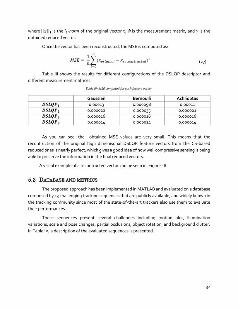
32
where ||𝑥||1 is the 𝑙1-norm of the original vector 𝑥, 𝛷 is the measurement matrix, and 𝑦 is the
obtained reduced vector.
Once the vector has been reconstructed, the MSE is computed as:
𝑀𝑆𝐸 = 1
𝑛∑(𝑥𝑜𝑟𝑖𝑔𝑖𝑛𝑎𝑙 − 𝑥𝑟𝑒𝑐𝑜𝑛𝑠𝑡𝑟𝑢𝑐𝑡𝑒𝑑)
2
𝑛
𝑖=0
Table III shows the results for different configurations of the DSLQP descriptor and
different measurement matrices.
Table III: MSE computed for each feature vector.
Gaussian Bernoulli Achlioptas
𝑫𝑺𝑳𝑸𝑷𝟏 0.00013 0.000098 0.00011
𝑫𝑺𝑳𝑸𝑷𝟐 0.000022 0.000035 0.000021
𝑫𝑺𝑳𝑸𝑷𝟒 0.000016 0.000016 0.000016
𝑫𝑺𝑳𝑸𝑷𝟖 0.000014 0.000014 0.000014
As you can see, the obtained MSE values are very small. This means that the
recontruction of the original high dimenisonal DSLQP feature vectors from the CS-based
reduced ones is nearly perfect, which gives a good idea of how well compressive sensing is being
able to preserve the information in the final reduced vectors.
A visual example of a recontructed vector can be seen in Figure 18.
5.3 DATABASE AND METRICS
The proposed approach has been implemented in MATLAB and evaluated on a database
composed by 13 challenging tracking sequences that are publicly available, and widely known in
the tracking community since most of the state-of-the-art trackers also use them to evaluate
their performances.
These sequences present several challenges including motion blur, illumination
variations, scale and pose changes, partial occlusions, object rotation, and background clutter.
In Table IV, a description of the evaluated sequences is presented.
(27)

33
Figure 18. Compressive Sensing reconstruction example.
DSLQP
descriptor
Dimensionality
reduction
Reconstruction
Absolute reconstruction error

34
Table IV: Database video sequences.
Video sequence Number of frames
Challenging factors Video resolution
Animal 71 Background clutter and abrupt motion
704x400
Cliffbar 327 Scale change, background clutter and abrupt motion.
320x240
David 263 Illumination changes, scale and pose change, background clutter.
320x240
Faceocc2 811 Occlusion, pose changes and background clutter
320x240
Football 362 Occlusion and background clutter 624x352
Girl 501 Occlusion, scale and pose changes 320x240
Jumping 313 Abrupt motion and blur 352x288
Shaking 365 Illumination changes, scale and pose changes, partial occlusion and
background clutter
624x352
Singer1 351 Illumination changes, scale change and background clutter
624x352
Skating1 400 Illumination changes, scale and pose change and background
clutter
640x360
Sylv 1343 Illumination changes, pose variation
320x240
Trellis 569 Illumination changes, scale changes and background clutter
320x240
Woman 597 Occlusion, scale change and similar object
352x288
The evaluation is performed by computing the misalignment between the ground truth
and the estimated target positions and sizes obtained by the tracker.
Specifically, the set of metrics that has been used for single object tracking is:
Success Rate (SR): evaluates the overlap between the tracking bounding box (𝑅𝑂𝐼 𝑇)
and the ground truth bounding box (𝑅𝑂𝐼 𝐺) using the equation:
𝑠𝑐𝑜𝑟𝑒 = 𝑎𝑟𝑒𝑎(𝑅𝑂𝐼 𝑇 ∩ 𝑅𝑂𝐼 𝐺 )
𝑎𝑟𝑒𝑎(𝑅𝑂𝐼 𝑇 ∪ 𝑅𝑂𝐼 𝐺 )
The maximum value of this score is 1, which occurs when the tracking bounding box and
the ground truth bounding box are exactly at the same location and have the same size.
(28)

35
To decide whether the tracker has successfully tracked the target, usually a 0.5 threshold
is used:
{𝑠𝑢𝑐𝑐𝑒𝑠𝑠 𝑖𝑓 𝑠𝑐𝑜𝑟𝑒 ≥ 0.5𝑒𝑟𝑟𝑜𝑟 𝑖𝑓 𝑠𝑐𝑜𝑟𝑒 ≤ 0.5
Thus, the SR score is finally obtained by computing the number of success scores divided
by the total number of frames.
Precision Rate (PR): is a measure to evaluate the ability of the tracker to accurately
estimate the object positions. This rate calculates the distance between the tracked
object and its ground truth for those frames where the tracking has been successful
according to the accuracy rate. It is calculated by:
𝑃𝑅 = ∑𝑑𝑖𝑠𝑡𝑎𝑛𝑐𝑒𝑠
𝑛º 𝑜𝑓 𝑠𝑢𝑐𝑐𝑒𝑠𝑠
Center Location Error (CLE): calculates the distance between the predicted center
position and the ground truth center position. The higher the distance, the higher the
deviation of the tracker result. Clearly, trackers expect CLE to be small. It is calculated
by:
𝐶𝐿𝐸 = √(𝑥𝑔𝑡 − 𝑥𝑝𝑟𝑒𝑑𝑖𝑐𝑡𝑒𝑑)2 + (𝑦𝑔𝑡 − 𝑦𝑝𝑟𝑒𝑑𝑖𝑐𝑡𝑒𝑑)2
The CLE and the PR both measure the distance between the predicted object position
and its ground truth, however PR only performs this measure when the tracking has been
rated as successful, given an idea of the accuracy of the successfully tracked frames.
5.4 EXPERIMENTAL RESULTS
The developed tracker has some important parameters that need to be fixed to reach an
optimal behavior. These parameters are related to the search regions, the SVM classifier, and
the feature extraction step.
The search regions are designed according to the bounding box of the target object that
is tracked. The positive samples for the training of the SVM are obtained from a region near the
current target location, more precisely the region that overlaps with the original bounding box
in at least 80%. Figure 19(a) shows an example. The negative samples are sampled form the
surrounding background near the object. This is obtained as the bounding box whose
overlapping with the original bounding box is between 10% and 80% (see Figure 19(b)).
For the positive sampling region, a Gaussian-sampling strategy is performed, whereas a
uniform sampling strategy is done for the negative sampling region. At each sampling step, a
maximum of 50 positive and negative samples are taken.
(29)
(30)
(31)
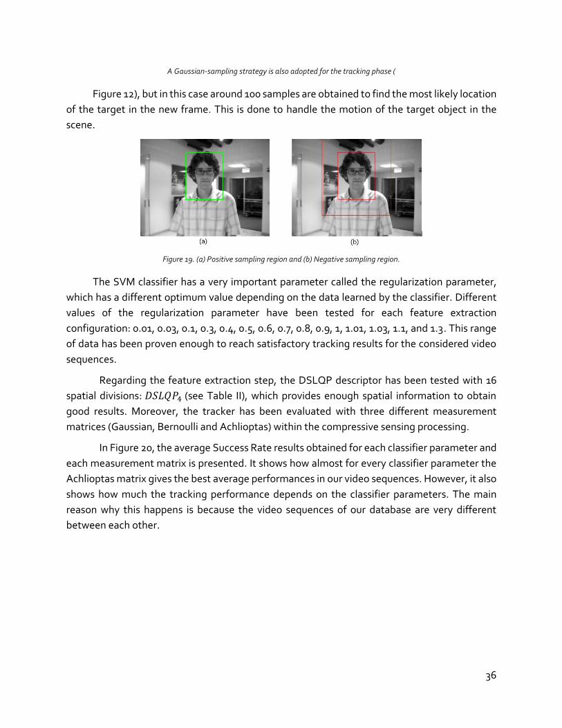
36
A Gaussian-sampling strategy is also adopted for the tracking phase (
Figure 12), but in this case around 100 samples are obtained to find the most likely location
of the target in the new frame. This is done to handle the motion of the target object in the
scene.
Figure 19. (a) Positive sampling region and (b) Negative sampling region.
The SVM classifier has a very important parameter called the regularization parameter,
which has a different optimum value depending on the data learned by the classifier. Different
values of the regularization parameter have been tested for each feature extraction
configuration: 0.01, 0.03, 0.1, 0.3, 0.4, 0.5, 0.6, 0.7, 0.8, 0.9, 1, 1.01, 1.03, 1.1, and 1.3. This range
of data has been proven enough to reach satisfactory tracking results for the considered video
sequences.
Regarding the feature extraction step, the DSLQP descriptor has been tested with 16
spatial divisions: 𝐷𝑆𝐿𝑄𝑃4 (see Table II), which provides enough spatial information to obtain
good results. Moreover, the tracker has been evaluated with three different measurement
matrices (Gaussian, Bernoulli and Achlioptas) within the compressive sensing processing.
In Figure 20, the average Success Rate results obtained for each classifier parameter and
each measurement matrix is presented. It shows how almost for every classifier parameter the
Achlioptas matrix gives the best average performances in our video sequences. However, it also
shows how much the tracking performance depends on the classifier parameters. The main
reason why this happens is because the video sequences of our database are very different
between each other.

37
Figure 20: Average Success Rate graphics.
Table V: Best Success Rate for each video sequence with each matrix evaluated
Table V shows the best Success Rate obtained for each video sequence with each
measurement matrix. As it can be observed, almost every sequence has at least one classifier
parameter for which our tracker gives good performances. However, there are three sequences
for which our tracker performs very poorly for every tested configuration. These sequences are
the Animal sequence, the Skating1 sequence and the Woman sequence. The Animal sequence
has a lot of blurring and abrupt motion that our tracker is not able to cope with. The reason is
that the used DSLQP descriptor is very discriminative for images with a minimum of resolution
and definition, but when dealing with low definition sequences that present a high degree of
Sequence
Developed Tracker
(Gaussian matrix)
Developed Tracker
(Bernoulli matrix)
Developed Tracker
(Achioptlas matrix)
Animal 0,0563 0,0563 0,0563
Cliffbar 0,8484 0,6363 0,8484
David 0,8289 0,9885 0,9924
Faceocc2 0,9012 0,858 0,8086
Football 0,7901 0,7623 0,9586
Girl 0,7327 0,8514 0,8514
Jumping 0,2076 0,9712 0,3003
Shaking 0,7781 0,4356 0,5095
Singer1 0,5498 0,7094 0,8832
Skating1 0,1375 0,15 0,18
Sylv 0,5018 0,6617 0,881
Trellis 0,427 0,9578 0,9666
Woman 0,1474 0,1675 0,1323
Median 0,5498 0,7094 0,8484
Mean 0,5313 0,6312 0,6437

38
blurring, the DSLQP descriptor is not able to characterize well the target appearance, and
consequently the tracker performance decreases. Moreover, the high motion of the object in
this sequence gives an extra drawback to the performance of our tracker. On the other hand, the
Skating1 sequence and the Woman sequence are videos with large variations in the object scale.
And the current design of the proposed tracker does not considered such a situation, since it
works with the same bounding box size for every frame of each video. Hence, it was expected
that our tracker could not handle this kind of changes.
In conclusion, the proposed tracker has a high performance in challenging sequences
with partial occlusion, illumination changes, pose variation, and background clutter, although
its performance can decrease with blurry images and large scale variations. In the following
figures (Figure 21-Figure 24), the performance of the proposed tracker is shown for some of the
most challenging frames of the video sequences: Cliffbar, Trellis, Sylv, and Jumping. The used
tracking parameters for these sequences along the SR score are presented in Table VI.
Table VI: Best parameters and results for Cliffbar, Trellis, Sylv and Jumping video sequences.
Measurement matrix
Classifier parameter Success Rate
Cliffbar Achlioptas 0,3 0,8484
Trellis Achlioptas 0,1 0,9666
Sylv Achlioptas 0,3 0,8810
Football Bernoulli 0,03 0,9972
Figure 21. Challenging frames in Cliffbar sequence

39
Figure 22. Challenging frames in Trellis sequence
Figure 23. Challenging frames in Sylv sequence
Figure 24. Challenging frames in Football sequence
5.4.1 Quantitative comparisons
In this section, we evaluate our developed tracking algorithm against 12 state-of-the-art
methods, described in Section 2.4. The tracking results of these 12 state-of-the-art-trackers has
been obtained from the results given by the original authors on their respective papers.
Table VII and Table VIII show the results for every tracking algorithm and sequence. Table
VII shows the Successful Rate scores, and Table VIII the Central Error Location. In addition the
two last rows of every table show the median and mean scores considering all the sequences.
Although a specific configuration of parameters should be desirable for processing all the videos,

40
the best parameters for each independent sequence have been considered for two reasons. The
first one is to have the same testing conditions regarding the evaluation of the other trackers,
and the second one is due to the huge difference in nature of the considered sequences of the
dataset.
As we can observed from Table VII, the Successful Rate score of the developed tracking
algorithm outperforms the other state-of-the-art trackers globally, and also individually for
most of the sequences. This is attributed to the efficacy of the proposed feature extraction
technique that combines the use of the DSLQP descriptor with the Compressed Sensing
technique. Regarding the Central Error Location shown in Table VIII, the proposed algorithm is
among the three ones that achieve the best scores, and therefore we can conclude that the
proposed algorithm not only tracks successfully the target objects, but also accurately.
Table IX shows the Success Rate scores again, but using a common set of tracking
parameters in the proposed algorithm in a subset of video sequences (the scores of the other
trackers are the same as the ones presented in Table VII), which is more challenging. In order to
obtain the best configuration of tracking parameters, the video sequences have been analyzed
separately. As a result, the David, Trellis, Cliffbar, Faceocc2, Football, and Sylv sequences present
similar challenging tasks: Illumination changes, partial occlusion, pose variation, and
background clutter. Since these challenges are the ones that our tracker has been designed for
(due to the DSLQP feature descriptor and the update model implemented), a common set of
tracking parameters have been estimated to maximize the performance in this subset of videos.
These parameters are: the Achlioptas matrix and a classifier parameter of 0.3.
Despite the fact that the used parameters are not the optimum for every sequence (unlike
the results of the other algorithms), the obtained Success Rate scores from the proposed
algorithm are still the best ones in most of the sequences. This fact proves the robustness and
efficiency of the designed tracking algorithm.

41
Table VII: Table with the Success Rate (%) results of 12-state-of-the-art trackers and our developed. The best results are shown in
red, blue and green fonts respectively.
Sequ
ence
Deve
loped
Trac
ker
IVT
Frag
MIL
VTD
LSST
Stru
ckCT
L1T
MTT
ONND
ASLA
SCM
Animal
0,056
30,2
166
0,076
40,2
129
0,577
10,5
750,6
062
0,525
0,038
60,5
185
0,625
70,6
198
0,608
1
Cliffb
ar0,8
484
0,564
80,1
337
0,462
20,3
292
0,564
80,6
580,3
852
0,199
30,3
073
0,348
30,6
197
0,653
3
David
0,992
30,7
116
0,194
60,4
479
0,525
20,7
671
0,444
20,4
342
0,625
0,288
80,4
131
0,643
0,671
2
Faceocc2
0,901
20,7
877
0,674
0,675
90,7
095
0,845
70,6
459
0,609
80,7
561
0,764
90,4
950,8
561
0,841
2
Football
0,997
20,1
269
0,521
0,576
0,557
30,6
886
0,525
70,6
994
0,573
20,6
643
0,407
60,6
362
0,830
8
Girl
0,851
40,4
305
0,688
80,5
189
0,511
0,121
10,0
103
0,512
40,3
296
0,633
80,4
218
0,650
50,6
795
Jump
ing0,9
712
0,282
60,1
383
0,526
70,0
797
0,654
0,581
90,1
531
0,092
70,2
318
0,135
70,7
121
0,717
4
Shaking
0,778
0,041
90,1
314
0,618
0,642
0,040
20,0
564
0,041
10,0
562
0,536
90,7
072
0,039
70,7
054
Singer1
0,883
20,6
622
0,340
90,3
372
0,79
0,798
70,3
913
0,342
10,7
043
0,415
40,2
026
0,799
50,8
668
Skating
10,1
80,0
246
0,089
90,1
206
0,574
30,1
341
0,297
80,0
543
0,091
0,089
60,2
028
0,495
70,5
358
Sylv
0,881
040,0
6777
0,494
80,5
548
0,587
20,2
80,6
430,5
801
0,398
70,6
464
0,674
90,1
298
0,691
6
Trellis
0,966
60,0
759
0,317
60,2
666
0,398
60,2
953
0,450
30,3
413
0,390
10,4
168
0,692
90,1
462
0,651
6
Wom
an0,1
675
0,047
0,127
0,129
0,118
10,1
622
0,569
30,1
202
0,126
20,1
251
0,194
70,7
929
0,172
8
Med
ian0,8
810
0,216
60,1
946
0,462
20,5
573
0,564
80,5
257
0,385
20,3
296
0,416
80,4
131
0,636
20,6
795
Mea
n0,7
288
0,310
80,3
022
0,419
00,4
922
0,455
90,4
523
0,369
10,3
370
0,433
80,4
248
0,549
30,6
635

42
Table VIII: Table with the Center Error Rate (%) results of 12-state-of-the-art trackers and our developed tracker. The best
results are shown in red, blue and green fonts respectively.
Sequ
ence
Deve
loped
Trac
ker
IVT
Frag
MIL
VTD
LSST
Stru
ckCT
L1T
MTT
ONND
ASLA
SCM
Animal
108,2
341
127,4
692
,088
66,45
611
,919
10,00
413
,547
19,84
917
1,46
15,85
58,4
425
7,173
410
,016
Cliffb
ar34
,8392
24,81
1248
,674
13,34
734
,555
23,30
67,9
976
23,42
49,6
46,17
1129
,606
5,605
87,7
062
David
10,50
243,5
893
76,69
116
,146
13,55
23,9
366
17,61
516
,471
7,629
914
3,29
23,47
63,6
578
5,344
Faceocc2
6,978
25,1
1912
,1189
11,74
547,3
731
3,629
912
,0866
17,98
137,1
772
5,935
321
,1782
3,257
64,3
644
Football
4,668
136
,952
17,21
113
,6613
,609
7,574
313
,927
8,138
118
,176
9,842
420
,366
14,93
93,8
996
Girl
16,08
47,90
318
,0618
32,29
421
,477
72,33
612
8,67
32,81
260
,9823
,876
27,74
916
,089,9
34
Jump
ing4,5
233
36,80
258
,448
9,894
162
,988
4,771
67,2
921
42,99
692
,393
34,47
336
,611
4,279
74,0
973
Shaking
13,33
3572
,5011
159,7
8113
,1808
11,65
1692
,0302
102,0
9514
9,433
112,6
8618
,258,5
778
71,30
099,1
428
Singer1
31,74
778,4
834
22,03
415
,174,0
567
3,506
113
,171
13,25
64,5
707
16,62
112
,344,6
693,5
024
Skating
148
,6582
113,7
0614
1,981
161,6
7513
,3276
120,0
1881
,9489
186,5
8916
3,672
195,6
17,3
027
26,63
615
,1529
Sylv
30,96
2168
,2206
20,08
7214
,5529
20,08
7284
,5988
9,329
613
,0829
23,63
868,9
906
8,087
544
,2741
7,225
4
Trellis
8,354
910
7,943
56,32
1768
,7835
,3769
85,70
4823
,341
41,20
6134
,3166
48,64
628,5
942
49,51
412
,8277
Wom
an10
7,141
619
7,97
100,4
112
4,511
118,4
9911
6,434
7,943
211
4,827
130,6
1513
4,016
7,111
42,4
206
143,5
9

43
Table IX: Table with the Success Rate (%) results in a selection of videos of the considered database. The best results are shown in
red, blue and green fonts respectively.
Sequ
ence
Deve
loped
Trac
ker
(Ach
ioptla
s 0,3)
IVTFra
gMI
LVT
DLSS
TStr
uck
CTL1
TMT
TON
NDAS
LASC
M
Cliffb
ar0,8
484
0,564
80,1
337
0,462
20,3
292
0,564
80,6
580,3
852
0,199
30,3
073
0,348
30,6
197
0,653
3
David
0,992
30,7
116
0,194
60,4
479
0,525
20,7
671
0,444
20,4
342
0,625
0,288
80,4
131
0,643
0,671
2
Faceocc2
0,796
30,7
877
0,674
0,675
90,7
095
0,845
70,6
459
0,609
80,7
561
0,764
90,4
950,8
561
0,841
2
Footb
all0,9
475
0,126
90,5
210,5
760,5
573
0,688
60,5
257
0,699
40,5
732
0,664
30,4
076
0,636
20,8
308
Sylv
0,881
00,0
6777
0,494
80,5
548
0,587
20,2
80,6
430,5
801
0,398
70,6
464
0,674
90,1
298
0,691
6
Trellis
0,869
90,0
759
0,317
60,2
666
0,398
60,2
953
0,450
30,3
413
0,390
10,4
168
0,692
90,1
462
0,651
6

44
6 CONCLUSION AND FUTURE WORK
In this work we have proposed a new visual object tracker that approaches the tracking
problem with a tracking-by-detection method that builds up an effective appearance model in
the compressed domain. Our algorithm trains an SVM classifier in an online fashion to separate
the object from the background. The appearance model is generated with a robust high
dimensional feature descriptor, the DSLQP descriptor, which describes the objects and the
surrounding background of the scene. In addition, due to the high computational cost and the
memory restrictions of such high dimensional vectors, a dimensionality reduction step based on
the compressed sensing theory has been added.
The compressive sensing theory has been exploited to implement a dimensionality
reduction step that assures that the information and geometrical relationships of the original
high dimensional vectors are preserved in the compressed ones. We have demonstrated its
success by analyzing our resultant vectors via a recovery algorithm, which shows that our low
dimensional vectors are able to recover the original vectors with a very low reconstruction error.
A successful update of the appearance model is also achieved by using the tracker
predictions to extract positive and negative samples, which are used to train at each frame the
classifier with these new samples. This way our tracker is able to adapt to the appearance
variation of the object in challenging sequences.
The proposed tracking algorithms has been implemented in MATLAB, and evaluated
with a series of challenging video sequences that have proven the success of the algorithm.
One of the main contributions of this work is the application of the Compressed Sensing
theory for projecting high dimensional sparse vectors into low dimensional ones, while
preserving almost all the information. Furthermore, it is also proven that the classifier in the
compressive domain achieves great performances. In this work, this concept has been
successfully applied to tracking, however, it could be also applied to many other detection
approaches, such as face or hand-gesture recognition algorithms, where the high computational
cost of certain feature vectors prevents their practical application.
Regarding the future work, two different lines have been selected. The first one is related
to the computational performance. This work is not a real-time tracking approach, which makes
it not very attractive to some applications. Therefore, this improvement is considered for further
investigations, suggesting that it could be improved by adapting the tracker to other more
computationally efficient programming language, and/or re-design the algorithm stages for
being less computationally demanding.

45
The second line of future work is related to the implemented SVM classifier. A great
improvement in the performance of our tracker could be achieved by carrying a more deeply
and thorough evaluation of the classifier regularization parameter. Moreover, in the literature,
many different kernels are proposed to successfully find the best hyperplane that separates the
data. The study of the use of other kernels could also be very useful to improve our tracking
performance. On the other hand, it could also be evaluated the use of other machine learning
approaches to learn high dimensional data, such as deep-learning, which is a recent machine
learning research area that focusses on learning high-level data representations.

46
REFERENCES
[1] S. Birchfield, "Elliptical head tracking using intensity gradients and color histograms," IEEE Computer Society Conference on Computer Vision and Pattern Recognition, 1998, pp.232-237.
[2] J. Lim, D. Kriegman, "Tracking humans using prior and learned representations of shape and appearance," IEEE International Conference on Automatic Face and Gesture Recognition, 2004, pp.869-874.
[3] K. Branson, S. Belongie, "Tracking multiple mouse contours (without too many samples)," IEEE Computer Society Conference on Computer Vision and Pattern Recognition, 2005, pp.1039-1046.
[4] H. Yang, L. Shao, F. Zheng, L. Wang, and Z. Song, "Recent advances and trends in visual tracking: A review, " Neurocomputing, Nov. 2011. vol. 74, no. 18, pp. 3823–3831.
[5] X. Mei, H. Ling, "Robust Visual Tracking and Vehicle Classification via Sparse Representation," IEEE Transactions on Pattern Analysis and Machine Intelligence, Nov 2011. vol.33, no.11, pp.2259-2272.
[6] N. D. Binh, "A Robust Framework for Visual Object Tracking," International Conference on Computing and Communication Technologies, 2009, pp.1-8.
[7] A. Yilmaz, O. Javed, and M. Shah, " Object Tracking: A Survey," ACM Computing Surveys, Dec. 2006.
[8] Y. Wu, J. Lim, M. H. Yang, "Online Object Tracking: A Benchmark," IEEE Conference on Computer Vision and Pattern Recognition, 2013, pp.2411-2418.
[9] T. Cootes, G. J. Edwards, and C. J. Taylor, "Active appearance models," European Conference on Computer Vision, 1998, pp. 484-498.
[10] D. Conte, P. Foggia, G. Percannella, and M. Vento, "A MultiView Appearance Model for people re-identification," IEEE International Conference on Advanced Video and Signal-Based Surveillance (AVSS), 2011, pp.297-302.
[11] A.W.M. Smeulders, D.M. Chu, R. Cucchiara, S. Calderara, A. Dehghan, and M. Shah, "Visual Tracking: An Experimental Survey," IEEE Transactions on Pattern Analysis and Machine Intelligence, July 2014. vol.36, no.7, pp.1442-1468.
[12] Z. Kalal, J. Matas, K. Mikolajczyk, "P-N learning: Bootstrapping binary classifiers by structural constraints," IEEE Conference on Computer Vision and Pattern Recognition, 2010, pp.49, 56, 13-18.
[13] B. Babenko, M. H. Yang, S. Belongie, "Robust Object Tracking with Online Multiple Instance Learning," IEEE Transactions on Pattern Analysis and Machine Intelligence, Aug. 2011, vol.33, no.8, pp.1619-1632.
[14] D. Comaniciu, V. Ramesh, P. Meer, "Kernel-based object tracking," IEEE Transactions on Pattern Analysis and Machine Intelligence, May 2003 , vol.25, no.5, pp.564-577.
[15] K. Levi, Y. Weiss, "Learning object detection from a small number of examples: the importance of good features," IEEE Computer Society Conference on Computer Vision and Pattern Recognition, 2004. vol.2, no., pp.II-53, II-60 Vol.2.
[16] N. Dalal, B. Triggs, "Histograms of oriented gradients for human detection," IEEE Computer Society Conference on Computer Vision and Pattern Recognition, 2005, pp.886-893.

47
[17] H. Grabner, M. Grabner and H. Bischof, "Real-Time Tracking via On-line Boosting,” Proceedings of the British Machine Conference, 2006, pp. 6.1-6.10.
[18] K. Zhang; L. Zhang; M. H. Yang, "Fast Compressive Tracking," IEEE Transactions on Pattern Analysis and Machine Intelligence, Oct. 1 2014 , vol.36, no.10, pp.2002-2015.
[19] D. G. Lowe, "Distinctive Image Features from Scale-Invariant Keypoints,” International Journal of Computer Vision, 2004, pp. 91-110.
[20] H. Bay, T. Tuytelaars, and L. Van Gool, "SURF: Speeded up robust features," European Conference on Computer Vision, 2006, pp.404-417.
[21] S. Hare, A. Saffari, P.H.S. Torr, "Struck: Structured output tracking with kernels," IEEE International Conference on Computer Vision, 2011, pp.263-270.
[22] D. Ross, J. Lim, R.-S. Lin, and M. H. Yang, "Incremental Learning for Robust Visual Tracking," International Journal of Computer Vision, 2008, pp. 125-141.
[23] D. Comaniciu, V. Ramesh, P. Meer, "Real-time tracking of non-rigid objects using mean shift," IEEE Conference on Computer Vision and Pattern Recognition, 2000, vol.2, pp.142-149.
[24] J. Li, J. Wang, "Adaptive object tracking algorithm based on eigenbasis space and compressive sampling," Image Processing, IET , Nov. 2012, vol.6, no.8, pp.1170-1180.
[25] R. Calderbank, S. Jafarpour, and R. Schapire, "Compressed Learning: Universal Sparse Dimensionality Reduction and Learning in the Measurement Domain," Technical report, Rice University, 2009.
[26] S.-J. Kim, K. Koh, M. Lustig, S. Boyd, and D. Gorinevsky, "An Inetrior-Point Method for Large-Scale l1-Regularized Least Squares," Proceedings International Conference on Image Processing, 2007, vol. 3, pp.117-120. http://www.stanford.edu/~boyd/l1_ls/
[27] M. A. Davenport, "Random observations on random observations: Sparse signal acquisition and processing, " Doctoral dissertation, Texas A&M University, Aug. 2010.
[28] R.G. Baraniuk, "Compressive Sensing," IEEE Signal Processing Magazine, July 2007, vol.24, no.4, pp.118-121.
[29] E.J. Candès, T. Tao, "Decoding by linear programming," IEEE Transactions on Information Theory, Dec. 2005, vol.51, no.12, pp.4203-4215.
[30] R. Baraniuk, M. Davenport, R. DeVore, and M. Wakin, "A simple proof of the restricted isometry property for random matrices," Springer Constructive Approximation, Dec. 2008, vol 28, pp.253-263.
[31] S. S. Chen, D. L. Donoho, and M. A. Saunders, "Atomic decomposition by Basis Pursuit,"
SIAM Review, 2001, vol. 43, pp.129-159.
[32] E. J. Candès, J. K. Romberg, and T. Tao, "Stable signal recovery from incomplete and inaccurate measurements," Communications on Pure and Applied Mathematics, March 2006, vol. 59, pp.1207-1223.
[33] E. Candes and J. Romberg, “‘L1-Magic: Recovery of Sparse Signals via Convex Programming,” http://www.acm.caltech.edu/l1magic/ , 2005.
[34] J.A. Tropp, "Greed is good: algorithmic results for sparse approximation," IEEE Transactions on Information Theory, Oct. 2004, vol.50, no.10, pp.2231-2242.

48
[35] M. A. Davenport, M. F. Duarte, Y. C. Eldar, and G. Kutyniok, (2011). "Introduction to compressed sensing," in Compressed Sensing: Theory and Applications. Cambridge University Press, 2011.
[36] T. Ojala, M. Pietikinen, and M. Harwood, "A comparative study of texture measures with classification based on featured distributions, " IEEE Computer Society Conference on Computer Vision and Pattern Recognition, 1996 , vol. 29, no. 1, pp. 51-59.
[37] R. Kasturi, D. Goldgof, P. Soundararajan, V. Manohar, J. Garofolo, R. Bowers, M. Boonstra, V. Korzhova, and J. Zhang, "Framework for Performance Evaluation of Face, Text, and Vehicle Detection and Tracking in Video: Data, Metrics, and Protocol," IEEE Transactions on Pattern Analysis and Machine Intelligence, Feb. 2009, vol.31, no.2, pp.319-336.
[38] K. Bernardin, and R. Stiefelhagen, "Evaluating multiple object tracking performance: the CLEAR MOT metrics, " Journal on Image and Video Processing, 2008.
[39] T. Mantecon, C.R. del-Bianco, F. Jaureguizar, N. and Garcia, "Depth-based face recognition using local quantized patterns adapted for range data," IEEE International Conference on Image Processing, Oct. 2014, vol., no., pp.293-297.
[40] E. Bingham, and H. Mannila, "Random projection in dimensionality reduction: applications to image and text data, " In Proceedings of the seventh ACM SIGKDD international conference on Knowledge discovery and data mining, Aug. 2001, pp. 245-250.
[41] A. Adam, E. Rivlin, I. Shimshoni, "Robust Fragments-based Tracking using the Integral Histogram," IEEE Computer Society Conference on Computer Vision and Pattern Recognition, June 2006, vol.1, no., pp.798-805.
[42] J. Kwon, and K. Mu Lee, "Visual tracking decomposition," IEEE Conference on Computer Vision and Pattern Recognition, June 2010 , pp.1269-1276.
[43] T. Zhang, B. Ghanem, S. Liu, and N. Ahuja, "Robust visual tracking via multi-task sparse learning," IEEE Conference on Computer Vision and Pattern Recognition, June 2012 ,pp.2042-2049.
[44] N. Wang; J. Wang; D. Y. Yeung, "Online Robust Non-negative Dictionary Learning for Visual Tracking," IEEE International Conference on Computer Vision, Dec. 2013, pp.657-664.
[45] W. Zhong, H. Lu, and M. H. Yang, "Robust object tracking via sparsity-based collaborative model," IEEE Conference on Computer Vision and Pattern Recognition, June 2012, pp.1838-1845.
[46] X. Jia, H. Lu, and M. H. Yang, "Visual tracking via adaptive structural local sparse appearance model," IEEE Conference on Computer Vision and Pattern Recognition, June 2012, pp.1822-1829.
[47] D. Wang, H. Lu, and M. H. Yang, "Least Soft-Threshold Squares Tracking," IEEE Conference on Computer Vision and Pattern Recognition, June 2013 , pp.2371-2378.
[48] S. Hare, A. Saffari, P.H.S. Torr, "Struck: Structured output tracking with kernels," IEEE International Conference on Computer Vision, Nov. 2011, pp.263-270.
[49] M. Danelljan, F.S. Khan, M. Felsberg, and J. van de Weijer, "Adaptive Color Attributes for Real-Time Visual Tracking," IEEE Conference on Computer Vision and Pattern Recognition, June 2014, pp.1090-1097.
[50] D. Achlioptas, "Database-friendly random projections: Johnson-Lindenstrauss with binary coins, " Journal of Computer and System Sciences - Special Issue on PODS, June 2003, vol.66, pp.671–687.


![MENDEZ] [CARLOS - carlos mendez](https://img.pdfslide.us/doc/110x75/620652ca8c2f7b173006a76f/mendez-carlos-carlos-mendez.jpg)