Trabajo de Estadística

DIANA PATRICIA ORTIZ

2060399

Frequency Table for ESTRATO

------------------------------------------------------------------------

Relative Cumulative Cum. Rel.

Class Value Frequency Frequency Frequency Frequency

------------------------------------------------------------------------

1 1 4 0,0800 4 0,0800

2 2 11 0,2200 15 0,3000

3 3 20 0,4000 35 0,7000

4 4 13 0,2600 48 0,9600

5 5 2 0,0400 50 1,0000

------------------------------------------------------------------------

The StatAdvisor

---------------

This table shows the number of times each value of ESTRATO

occurred, as well as percentages and cumulative statistics. For

example, in 4 rows of the data file ESTRATO equaled 1. This

represents 8,0% of the 50 values in the file. The rightmost two

columns give cumulative counts and percentages from the top of the

table down.

ESTRATO

0 4 8 12 16 20

frequency

1

2

3

4

5

ESTRATO

ESTRATO12345

8,00%

22,00%

40,00%

26,00%

4,00%

Análisis:

Se define que una empresa comercializadora de energía toma sus datos del estrato 1 al 5 y tenemos que en el estrato 1 hay 8,00%, el estrato 2 el 22,00%, estrato 3 40,00%, estrato 4 el 26,00% y el estrato 5 4,00%5.

Estos son los valores de cada estrato de la energía que produce cada uno.

# PERSONAS POR HOGAR

Analysis Summary

Data variable: # PERSONAS POR HOGAR

50 values ranging from 3,0 to 7,0

The StatAdvisor

---------------

This procedure is designed to summarize a single sample of data.

It will calculate various statistics and graphs. Also included in the

procedure are confidence intervals and hypothesis tests. Use the

Tabular Options and Graphical Options buttons on the analysis toolbar

to access these different procedures.

Summary Statistics for # PERSONAS POR HOGAR

Count = 50

Average = 5,1

Median = 5,0

Variance = 1,31633

Standard deviation = 1,14731

Minimum = 3,0

Maximum = 7,0

Range = 4,0

Lower quartile = 4,0

Upper quartile = 6,0

Stnd. skewness = -0,0975232

Stnd. kurtosis = -0,648362

The StatAdvisor

---------------

This table shows summary statistics for # PERSONAS POR HOGAR. It

includes measures of central tendency, measures of variability, and

measures of shape. Of particular interest here are the standardized

skewness and standardized kurtosis, which can be used to determine

whether the sample comes from a normal distribution. Values of these

statistics outside the range of -2 to +2 indicate significant

departures from normality, which would tend to invalidate any

statistical test regarding the standard deviation. In this case, the

standardized skewness value is within the range expected for data from

a normal distribution. The standardized kurtosis value is within the

range expected for data from a normal distribution.

Percentiles for # PERSONAS POR HOGAR

1,0% = 3,0

5,0% = 3,0

10,0% = 3,5

25,0% = 4,0

50,0% = 5,0

75,0% = 6,0

90,0% = 7,0

95,0% = 7,0

99,0% = 7,0

The StatAdvisor

---------------

This pane shows sample percentiles for # PERSONAS POR HOGAR. The

percentiles are values below which specific percentages of the data

are found. You can see the percentiles graphically by selecting

Quantile Plot from the list of Graphical Options.

Percentiles for # PERSONAS POR HOGAR

1,0% = 3,0

5,0% = 3,0

10,0% = 3,5

25,0% = 4,0

50,0% = 5,0

75,0% = 6,0

90,0% = 7,0

95,0% = 7,0

99,0% = 7,0

The StatAdvisor

---------------

This pane shows sample percentiles for # PERSONAS POR HOGAR. The

percentiles are values below which specific percentages of the data

are found. You can see the percentiles graphically by selecting

Quantile Plot from the list of Graphical Options.

Frequency Tabulation for # PERSONAS POR HOGAR

--------------------------------------------------------------------------------

Lower Upper Relative Cumulative Cum. Rel.

Class Limit Limit Midpoint Frequency Frequency Frequency Frequency

--------------------------------------------------------------------------------

at or below 2,8 0 0,0000 0 0,0000

1 2,8 3,51429 3,15714 5 0,1000 5 0,1000

2 3,51429 4,22857 3,87143 8 0,1600 13 0,2600

3 4,22857 4,94286 4,58571 0 0,0000 13 0,2600

4 4,94286 5,65714 5,3 21 0,4200 34 0,6800

5 5,65714 6,37143 6,01429 9 0,1800 43 0,8600

6 6,37143 7,08571 6,72857 7 0,1400 50 1,0000

7 7,08571 7,8 7,44286 0 0,0000 50 1,0000

above 7,8 0 0,0000 50 1,0000

--------------------------------------------------------------------------------

Mean = 5,1 Standard deviation = 1,14731

The StatAdvisor

---------------

This option performs a frequency tabulation by dividing the range

of # PERSONAS POR HOGAR into equal width intervals and counting the

number of data values in each interval. The frequencies show the

number of data values in each interval, while the relative frequencies

show the proportions in each interval. You can change the definition

of the intervals by pressing the alternate mouse button and selecting

Pane Options. You can see the results of the tabulation graphically

by selecting Frequency Histogram from the list of Graphical Options.

DIAGRAMA DE CAJA

# PERSONAS POR HOGAR3 4 5 6 7

HISTOGRAMA

# PERSONAS POR HOGAR

freq

uenc

y

2,8 3,8 4,8 5,8 6,8 7,80

4

8

12

16

20

24

Analysis:

Estos son los datos del Número de Personas por hogar que consumen energía, donde se muestra los percentiles y la tabla tabulando los datos.

CONSUMO MENSUAL EN KW-H

Analysis Summary

Data variable: CONS KHM


The StatAdvisor

---------------






Summary Statistics for CONS KHM

Count = 50

Average = 99,756

Median = 96,95

Variance = 602,045


Minimum = 48,0

Maximum = 153,4

Range = 105,4



Stnd. skewness = 0,690105


The StatAdvisor

---------------

This table shows summary statistics for CONS KHM. It includes

measures of central tendency, measures of variability, and measures of

shape. Of particular interest here are the standardized skewness and

standardized kurtosis, which can be used to determine whether the

sample comes from a normal distribution. Values of these statistics

outside the range of -2 to +2 indicate significant departures from

normality, which would tend to invalidate any statistical test

regarding the standard deviation. In this case, the standardized

skewness value is within the range expected for data from a normal

distribution. The standardized kurtosis value is within the range

expected for data from a normal distribution.

Percentiles for CONS KHM

1,0% = 48,0

5,0% = 65,7

10,0% = 69,0

25,0% = 83,6

50,0% = 96,95

75,0% = 120,1

90,0% = 136,05

95,0% = 141,1

99,0% = 153,4

The StatAdvisor

---------------

This pane shows sample percentiles for CONS KHM. The percentiles

are values below which specific percentages of the data are found.

You can see the percentiles graphically by selecting Quantile Plot

from the list of Graphical Options.

Frequency Tabulation for CONS KHM

--------------------------------------------------------------------------------



--------------------------------------------------------------------------------

at or below 40,0 0 0,0000 0 0,0000

1 40,0 57,1429 48,5714 1 0,0200 1 0,0200

2 57,1429 74,2857 65,7143 8 0,1600 9 0,1800

3 74,2857 91,4286 82,8571 11 0,2200 20 0,4000

4 91,4286 108,571 100,0 12 0,2400 32 0,6400

5 108,571 125,714 117,143 10 0,2000 42 0,8400

6 125,714 142,857 134,286 6 0,1200 48 0,9600

7 142,857 160,0 151,429 2 0,0400 50 1,0000

above 160,0 0 0,0000 50 1,0000

--------------------------------------------------------------------------------


The StatAdvisor

---------------


of CONS KHM into equal width intervals and counting the number of data

values in each interval. The frequencies show the number of data

values in each interval, while the relative frequencies show the

proportions in each interval. You can change the definition of the

intervals by pressing the alternate mouse button and selecting Pane

Options. You can see the results of the tabulation graphically by

selecting Frequency Histogram from the list of Graphical Options.

Box-and-Whisker Plot

40 60 80 100 120 140 160

CONS KHM

Histogram

40 60 80 100 120 140 160

CONS KHM

0

2

4

6

8

10

12

fre

qu

en

cy

COCINA CON GAS

Analysis Summary

Data variable: C GAS

Number of observations: 50

Number of unique values: 2

The StatAdvisor

---------------

This procedure counts the number of times each of the 2 unique

values of C GAS occurs. It then displays tables and graphs of the

tabulation.

Frequency Table for C GAS

------------------------------------------------------------------------



------------------------------------------------------------------------

1 No 15 0,3000 15 0,3000

2 Si 35 0,7000 50 1,0000

------------------------------------------------------------------------

The StatAdvisor

---------------

This table shows the number of times each value of C GAS occurred,

as well as percentages and cumulative statistics. For example, in 15

rows of the data file C GAS equaled No. This represents 30,0% of the

50 values in the file. The rightmost two columns give cumulative

counts and percentages from the top of the table down.

COCINA CON GAS

0 10 20 30 40

frequency

No

Si

COCINA CON GAS

C GASNoSi

30,00%

70,00%

No. de ELECTRODOMESTICOS EN EL HOGAR

Analysis Summary

Data variable: # ELECT H


The StatAdvisor

---------------






Summary Statistics for # ELECT H

Count = 50

Average = 3,14

Median = 3,0

Variance = 1,34735


Minimum = 1,0

Maximum = 5,0

Range = 4,0



Stnd. skewness = -0,347881


The StatAdvisor

---------------

This table shows summary statistics for # ELECT H. It includes

measures of central tendency, measures of variability, and measures of

shape. Of particular interest here are the standardized skewness and






skewness value is within the range expected for data from a normal

distribution. The standardized kurtosis value is within the range


Percentiles for # ELECT H

1,0% = 1,0

5,0% = 1,0

10,0% = 1,5

25,0% = 2,0

50,0% = 3,0

75,0% = 4,0

90,0% = 5,0

95,0% = 5,0

99,0% = 5,0

The StatAdvisor

---------------

This pane shows sample percentiles for # ELECT H. The percentiles

are values below which specific percentages of the data are found.

You can see the percentiles graphically by selecting Quantile Plot

from the list of Graphical Options.

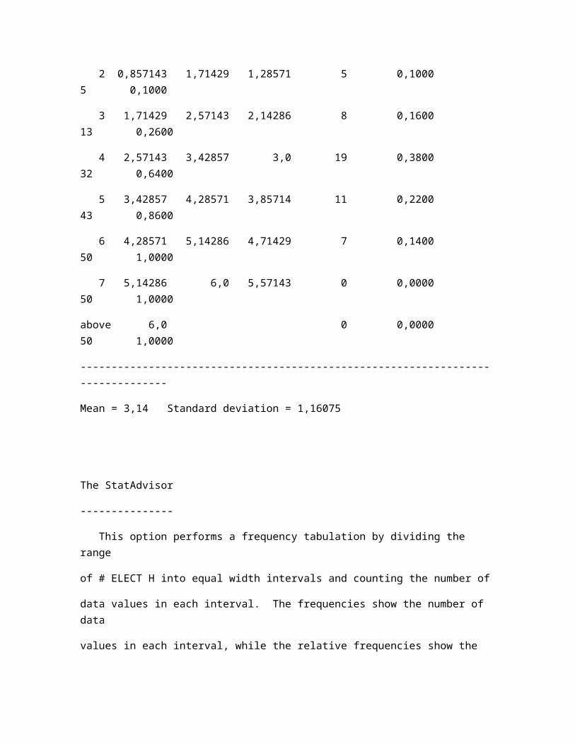
Frequency Tabulation for # ELECT H

--------------------------------------------------------------------------------



--------------------------------------------------------------------------------

at or below 0,0 0 0,0000 0 0,0000

1 0,0 0,857143 0,428571 0 0,0000 0 0,0000

2 0,857143 1,71429 1,28571 5 0,1000 5 0,1000

3 1,71429 2,57143 2,14286 8 0,1600 13 0,2600

4 2,57143 3,42857 3,0 19 0,3800 32 0,6400

5 3,42857 4,28571 3,85714 11 0,2200 43 0,8600

6 4,28571 5,14286 4,71429 7 0,1400 50 1,0000

7 5,14286 6,0 5,57143 0 0,0000 50 1,0000

above 6,0 0 0,0000 50 1,0000

--------------------------------------------------------------------------------


The StatAdvisor

---------------


of # ELECT H into equal width intervals and counting the number of

data values in each interval. The frequencies show the number of data






Box-and-Whisker Plot

0 1 2 3 4 5

# ELECT H

Histogram

0 1 2 3 4 5 6

# ELECT H

0

4

8

12

16

20

fre

qu

en

cy

GENERO DE PERSONAS QUE RESPONDEN LA ENCUESTA

Analysis Summary

Data variable: GPERS



The StatAdvisor

---------------


values of GPERS occurs. It then displays tables and graphs of the

tabulation.

Frequency Table for GPERS

------------------------------------------------------------------------



------------------------------------------------------------------------

1 F 34 0,6800 34 0,6800

2 M 16 0,3200 50 1,0000

------------------------------------------------------------------------

The StatAdvisor

This table shows the number of times each value of GPERS occurred,


rows of the data file GPERS equaled F. This represents 68,0% of the

50 values in the file. The rightmost two columns give cumulative

counts and percentages from the top of the table down.

GENERO DE PERSONAS

frequency0 10 20 30 40

F

M

GENERO DE PERSONAS

GPERSFM

68,00%

32,00%

CALIFICACION DEL SERIVICIO

Analysis Summary

Data variable: CSERV



The StatAdvisor

---------------


values of CSERV occurs. It then displays tables and graphs of the

tabulation.

Frequency Table for CSERV

------------------------------------------------------------------------



------------------------------------------------------------------------

1 1 4 0,0800 4 0,0800

2 2 13 0,2600 17 0,3400

3 3 21 0,4200 38 0,7600

4 4 8 0,1600 46 0,9200

5 5 4 0,0800 50 1,0000

------------------------------------------------------------------------

The StatAdvisor

---------------

This table shows the number of times each value of CSERV occurred,


rows of the data file CSERV equaled 1. This represents 8,0% of the 50

values in the file. The rightmost two columns give cumulative counts

and percentages from the top of the table down.

C ALIFICACION DEL SERVICIO

0 4 8 12 16 20 24

frequency

1

2

3

4

5

CALIFICACION DEL SERVICIO

CSERV12345

8,00%

26,00%

42,00%

16,00%

8,00%

INGRESO FAMILIAR MENSUAL

Analysis Summary

Data variable: IFM


The StatAdvisor

---------------






Summary Statistics for IFM

Count = 50

Average = 740,24

Median = 703,6

Variance = 46100,9


Minimum = 594,8

Maximum = 1790,6

Range = 1195,8



Stnd. skewness = 12,8455

Stnd. kurtosis = 28,7553

The StatAdvisor

---------------

This table shows summary statistics for IFM. It includes measures

of central tendency, measures of variability, and measures of shape.

Of particular interest here are the standardized skewness and






skewness value is not within the range expected for data from a normal

distribution. The standardized kurtosis value is not within the range


Percentiles for IFM

1,0% = 594,8

5,0% = 611,2

10,0% = 629,25

25,0% = 667,3

50,0% = 703,6

75,0% = 733,0

90,0% = 775,95

95,0% = 813,7

99,0% = 1790,6

The StatAdvisor

---------------

This pane shows sample percentiles for IFM. The percentiles are

values below which specific percentages of the data are found. You

can see the percentiles graphically by selecting Quantile Plot from

the list of Graphical Options.

Frequency Tabulation for IFM

--------------------------------------------------------------------------------



--------------------------------------------------------------------------------

at or below 500,0 0 0,0000 0 0,0000

1 500,0 714,286 607,143 32 0,6400 32 0,6400

2 714,286 928,571 821,429 16 0,3200 48 0,9600

3 928,571 1142,86 1035,71 0 0,0000 48 0,9600

4 1142,86 1357,14 1250,0 0 0,0000 48 0,9600

5 1357,14 1571,43 1464,29 0 0,0000 48 0,9600

6 1571,43 1785,71 1678,57 1 0,0200 49 0,9800

7 1785,71 2000,0 1892,86 1 0,0200 50 1,0000

above 2000,0 0 0,0000 50 1,0000

--------------------------------------------------------------------------------


The StatAdvisor

---------------


of IFM into equal width intervals and counting the number of data

values in each interval. The frequencies show the number of data






DIAGRAMA DE CAJA

500 800 1100 1400 1700 2000

IFM

HISTOGRAMA

500 800 1100 1400 1700 2000

IFM

0

10

20

30

40

fre

qu

en

cy

Documents

Trabajo de Estadística