MITSUBISHI ELECTRIC RESEARCH LABORATORIEShttp://www.merl.com

On the Performance of LinearLeast-Squares Estimation in Wireless

Positioning Systems

Sinan Gezici, Ismail Guvenc, Zafer Sahinoglu

TR2008-025 June 2008

Abstract

A common technique for wireless positioning is to estimate time-of-arrivals (TOAs) of signalstraveling between a target node and a number of reference nodes, and then to determine theposition of the target node based on those TOA parameters. In determining the position of thetarget node from TOA parameters, linear or nonlinear least-squares (LS) estimation techniquescan be employed. Although the linear LS techniques are suboptimal in general, they facilitatelow-complexity position estimation. In this paper, performance of various linear LS techniquesare compared, and suboptimality of the linear approach is quantified in terms of the Cramer-Raolower bound (CRLB). Simulations are performed to compare the performance of the linear LSapproaches versus the CRLBs for linear and nonlinear techniques.

ICC 2008 (May)

This work may not be copied or reproduced in whole or in part for any commercial purpose. Permission to copy in whole or in partwithout payment of fee is granted for nonprofit educational and research purposes provided that all such whole or partial copies includethe following: a notice that such copying is by permission of Mitsubishi Electric Research Laboratories, Inc.; an acknowledgment ofthe authors and individual contributions to the work; and all applicable portions of the copyright notice. Copying, reproduction, orrepublishing for any other purpose shall require a license with payment of fee to Mitsubishi Electric Research Laboratories, Inc. Allrights reserved.

Copyright c©Mitsubishi Electric Research Laboratories, Inc., 2008201 Broadway, Cambridge, Massachusetts 02139

MERLCoverPageSide2

1

On the Performance of Linear Least-SquaresEstimation in Wireless Positioning Systems

Sinan Gezici∗, Ismail Guvenc], and Zafer Sahinoglu‡

∗ Department of Electrical and Electronics Engineering, Bilkent University, Bilkent, Ankara 06800, Turkey] DoCoMo Communications Laboratories USA, Inc., 3240 Hillview Avenue, Palo Alto, CA 94304, USA‡ Mitsubishi Electric Research Laboratories, 201 Broadway Avenue, Cambridge, MA 02139, USA

Email: gezici@ee.bilkent.edu.tr, iguvenc@docomolabs-usa.com, zafer@merl.com

Abstract— A common technique for wireless positioning is toestimate time-of-arrivals (TOAs) of signals traveling betweena target node and a number of reference nodes, and thento determine the position of the target node based on thoseTOA parameters. In determining the position of the target nodefrom TOA parameters, linear or nonlinear least-squares (LS)estimation techniques can be employed. Although the linearLS techniques are suboptimal in general, they facilitate low-complexity position estimation. In this paper, performance ofvarious linear LS techniques are compared, and suboptimalityof the linear approach is quantified in terms of the Cramer-Raolower bound (CRLB). Simulations are performed to compare theperformance of the linear LS approaches versus the CRLBs forlinear and nonlinear techniques.

Index Terms— Wireless positioning, time-of-arrival (TOA),least-squares (LS) estimation, Cramer-Rao lower bound (CRLB).

I. INTRODUCTION

The subject of positioning in wireless systems has beendrawing considerable attention due to its potential applicationsand services for both cellular and short-range systems [1],[2]. For cellular systems, enhanced-911, improved fraud de-tection, location sensitive billing, intelligent transport systemsand improved traffic management can become feasible withaccurate positioning [1], [3]. On the other hand, for short-rangenetworks, position estimation facilitates applications such asinventory tracking, intruder detection, tracking of fire-fightersand miners, home automation and patient monitoring [4], [5].These potential applications of wireless positioning were alsorecognized by the IEEE, which approved a new amendment,IEEE 802.15.4a, that provides a new physical layer for lowdata rate communications combined with positioning capabil-ities [6]-[8]. Also, the Federal Communications Commission(FCC) in the U.S. required wireless providers to estimate theposition of mobile users within tens of meters for emergency911 calls [9].

A common approach in wireless positioning systems in-volves estimation of position in two steps. In the first step,position related parameters, such as time-of-arrivals (TOAs) ofsignals traveling between the target node, i.e. the node to belocated, and a number of reference nodes are estimated. Then,in the second step, the position is estimated based on the signalparameters obtained in the first step [3]. The position relatedparameters estimated in the first step are commonly TOA orreceived signal strength (RSS) parameters, which provide an

estimate for the distance between two nodes, or angle-of-arrival (AOA) parameters, which estimate the angles betweenthe nodes [1]. For distance based positioning algorithms, suchas TOA or RSS based schemes, the maximum likelihood(ML) solution can be obtained by a nonlinear least-squares(N-LS) approach, under certain conditions [10]. The N-LSapproach requires the minimization of a cost function thatrequires numerical search methods such as the steepest descentor the Gauss-Newton techniques. Such techniques can havehigh computational complexity and they typically require goodinitialization in order to avoid converging to the local minimaof the cost function [11].

In order to obtain a closed-form solution and avoid computa-tional complexity of the N-LS approach, the set of expressionscorresponding to the position related parameter estimates canbe linearized using the Taylor series expansion [12]. How-ever, such an approach still requires an intermediate positionestimate to obtain the Jacobian matrix, which should besufficiently close to the true position of the target node forthe linearity assumption to hold. Alternatively, a linear least-squares (L-LS) approach based on the measured distances wasinitially proposed in [13]. In the L-LS approach, the expressioncorresponding to one of the reference nodes is subtracted fromall the other expressions in order to obtain linear relationsin terms of the target node position. Various versions of theL-LS approach are studied in [14] and [15], which subtractdifferent expressions or average of them from the remainingexpressions.

The L-LS approach is a suboptimal positioning technique,which provides a solution with low computational complexity.Therefore, it can be employed for applications that require lowcost/complexity implementation with reasonable positioningaccuracy. In addition, for applications that require preciseposition estimation, L-LS approaches can be used to obtain aninitial position estimate for initializing high-accuracy position-ing algorithms, such as the N-LS approach and linearizationbased on the Taylor series [16]. A good initialization cansignificantly decrease the computational complexity and thefinal localization error of a high-accuracy technique. There-fore, performance analysis of the L-LS approaches is importantfrom multiple perspectives.

Although theoretical mean square errors (MSEs) of the L-LS approach are derived for various scenarios in [17], nostudies have considered the theoretical lower bounds that

2

can be achieved when using linearized measurements. In thispaper, performance of L-LS techniques for position estimationis investigated. Specifically, a closed-form approximate expres-sion for the Cramer-Rao lower bound (CRLB) is obtained forposition estimation based on linearized measurements. Then,it is shown that the bound applies to various L-LS approachesproposed in the literature. In addition, the performance ofthe L-LS algorithms is compared against each other andthe CRLBs for the linear and nonlinear models. Practicalimplications of the performance analysis are investigated.

The remainder of the paper is organized as follows. InSection II, the system model is defined, and measurementmodels are introduced. Then, the N-LS estimation and itsCRLB are briefly reviewed in Section III. In Section IV,the L-LS approaches are studied and their CRLB is derived.Finally, the simulation results are presented in Section V, andconcluding remarks are made in Section VI.

II. SYSTEM MODEL

Consider a wireless network with N reference nodes, withthe ith node being located at li = [xi yi]T for i = 1, . . . , N .The aim is to estimate the position of the target node, denotedby l = [x y]T , based on N TOA measurements between thetarget node and the reference nodes1.

Let zi represent the distance estimate obtained from the ithTOA measurement:

zi = c τi = fi(x, y) + ni, i = 1, . . . , N (1)

where τi represents the TOA estimate for the ith signal, c isthe speed of light, ni is the noise in the ith measurement, andfi(x, y) is the true distance between the target node and theith reference node, given by

fi(x, y) =√

(x− xi)2 + (y − yi)2 . (2)

Commonly, the noise is modeled by a zero-mean Gaussianrandom variable, when the reference node and the targetnode has direct line-of-sight (LOS). However, in non-line-of-sight (NLOS) conditions, the noise distribution can be quitedifferent from a Gaussian distribution [18], [19].

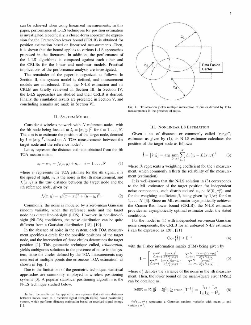
In the absence of noise in the system, each TOA measure-ment specifies a circle for the possible positions of the targetnode, and the intersection of those circles determines the targetposition [1]. This geometric technique called, trilateration,yields ambiguous solutions in the presence of noise in the sys-tem, since the circles defined by the TOA measurements mayintersect at multiple points due erroneous TOA estimation, asshown in Fig. 1.

Due to the limitations of the geometric technique, statisticalapproaches are commonly employed in wireless positioningsystems [3]. A popular statistical positioning algorithm is theN-LS technique studied below.

1In fact, the results can be applied to any systems that estimate distancesbetween nodes, such as a received signal strength (RSS) based positioningsystem, which performs distance estimation based on received signal energy[1].

Fig. 1. Trilateration yields multiple intersection of circles defined by TOAmeasurements in the presence of noise.

III. NONLINEAR LS ESTIMATION

Given a set of distance, or commonly called “range”,estimates as given by (1), an N-LS estimator calculates theposition of the target node as follows:

l =[x y

]= arg min

(x,y)

N∑

i=1

βi (zi − fi(x, y))2 (3)

where βi represents a weighting coefficient for the i measure-ment, which commonly reflects the reliability of the measure-ment (estimation).

It is well-known that the N-LS solution in (3) correspondsto the ML estimator of the target position for independentnoise components, each distributed as2 ni ∼ N (0 , σ2

i ), andfor the weighting coefficient βi being given by 1/σ2

i for i =1, . . . , N [3]. Since an ML estimator asymptotically achievesthe Cramer-Rao lower bound (CRLB), the N-LS estimatorprovides an asymptotically optimal estimator under the statedconditions.

For the model in (1) with independent zero-mean Gaussiannoise components, the CRLB for an unbiased N-LS estimatorl can be expressed as [20], [21]

Cov{l} ≥ I−1 (4)

with the Fisher information matrix (FIM) being given by

I =

∑Ni=1

(x−xi)2

σ2i f2

i (x,y)

∑Ni=1

(x−xi)(y−yi)σ2

i f2i (x,y)∑N

i=1(x−xi)(y−yi)

σ2i f2

i (x,y)

∑Ni=1

(y−yi)2

σ2i f2

i (x,y)

(5)

where σ2i denotes the variance of the noise in the ith measure-

ment. Then, the lower bound on the mean-square error (MSE)can be obtained as

MSE = E{‖l− l‖2} ≥ trace{I−1

}=

I11 + I22I11I22 − I212

(6)

2N (µ , σ2) represents a Gaussian random variable with mean µ andvariance σ2.

3

where Iij represents the element of I in the ith row and jthcolumn. From (5), I11 + I22 can be shown to be equal to∑N

i=1 σ−2i .

Since the N-LS estimator in (3) can asymptotically achievethe minimum MSE (MMSE) in (6) under certain conditions, itprovides a benchmark for the performance of other estimators.The main disadvantage of the N-LS estimator is related to thenonlinear nature of the optimization problem, which increasesits computational complexity. The common techniques forobtaining the N-LS estimator in (3) include gradient descentalgorithms and linearization techniques via the Taylor seriesexpansion [1], [12].

IV. LINEAR LS APPROACH AND CRLB ANALYSIS

A. Linear LS Estimation

An alternative approach to the N-LS estimation is the L-LS approach [13]-[15], [22]. In an L-LS technique, a newmeasurement set is obtained from the measurements in (1) bycertain operations that result in linear relations.

The L-LS approach starts with the following set of equations

z2i = (x− xi)2 + (y − yi)2, for i = 1, . . . , N , (7)

where each distance measurement is assumed to define acircle of uncertain region [22]. Then, one of the equationsin (7), say the rth one, is fixed and subtracted from all of theother equations. After some manipulation, the following linearrelation can be obtained [22]:

A l = p , (8)

where l = [x y]T ,

A = 2

x1 − xr y1 − yr

......

xr−1 − xr yr−1 − yr

xr+1 − xr yr+1 − yr

......

xN − xr yN − yr

, (9)

and

p =

z2r − z2

1 − kr + k1

...z2r − z2

r−1 − kr + kr−1

z2r − z2

r+1 − kr + kr+1

...

z2r − z2

N − kr + kN

, (10)

with

ki = x2i + y2

i , (11)

for i = 1, 2, . . . , N , and r being the selected reference nodeindex that is used to obtain linear relations. Note that A isan (N − 1) × 2 matrix, and p is a vector of size (N − 1),

since the rth measurement is used as a reference for the othermeasurements.

From (8), the LS solution can be obtained as

l = (AT A)−1AT p . (12)

This estimator is called the linear LS (L-LS) estimator. Com-pared to the N-LS estimator in (3), it has low computationalcomplexity. However, it is suboptimal in general, and theamount of its suboptimality can be quantified in terms theCRLB.

B. CRLB Analysis

In order to derive the CRLB for the L-LS approach, we firstmake the observation from (8)-(12) that the L-LS algorithmutilizes the measurements zi, i = 1, . . . , N , only through theterms z2

r − z2i , for i = 1, . . . , N and i 6= r. Therefore, the

measurement set for the L-LS algorithm effectively becomes

zi = z2r − z2

i, (13)

for i = 1, . . . , N − 1, where

i =

{i , i < r

i + 1 , i ≥ r. (14)

Let r = N without loss of generality and z represent thevector consisting of zi’s in (13); i.e.,

z =[z2N − z2

1 z2N − z2

2 · · · z2N − z2

N−1

]. (15)

In order to calculate the CRLB for any unbiased estimator thatemploys the observation (measurement set) z, we first need toobtain the conditional probability density function (PDF) of zgiven the location of the target node l.

From (1), (2) and (13), zi can be expressed as

zi = kN − ki + 2(xi − xN )x + 2(yi − yN )y

+ 2nNfN (x, y)− 2nifi(x, y) + (n2N − n2

i ) , (16)

for i = 1, . . . , N − 1, where ki and fi(x, y) are as in (11)and (2), respectively. In order to obtain a closed-form CRLBexpression, the last term in (16), namely n2

N −n2i , is modeled

as a Gaussian random variable. In other words, conditionedon l = [x y]T , zi in (16) is approximated by a Gaussiandistribution. This approximation gets quite accurate whenthe noise variance is considerably smaller than the distancesbetween the nodes. In general, it is expected that the CRLB tobe obtained under this approximate model provides a smallerbound than the exact model. In other words, a smaller CRLBis obtained by the Gaussian approximation, but the differencebetween the approximate and the exact models diminishes forsmall noise terms.

According to the model in (16), the conditional PDF of zi

given l = [x y]T can be obtained, after some manipulation, as

zi | l ∼ N(µi(x, y) , σi(x, y)

), (17)

where

µi(x, y) = f2N (x, y)− f2

i (x, y) + σ2N − σ2

i , (18)

σi(x, y) = 4[σ2

Nf2N (x, y) + σ2

i f2i (x, y)

]+ 2

(σ4

N + σ4i

).

(19)

4

In addition, the covariance terms can be calculated as3

E {(zi − µi)(zj − µj)} = 4σ2Nf2

N (x, y) + 2σ4N , (20)

for i 6= j. Then, the conditional distribution of z given l canbe expressed as

z | l ∼ N(

µ(x, y) , Σ(x, y))

, (21)

where

µ(x, y) =

µ1(x, y)µ2(x, y)

...µN−1(x, y)

, (22)

with µi(x, y) being given by (18) for i = 1, . . . , N − 1, and

Σ(x, y) =(4σ2

Nf2N (x, y) + 2σ4

N

)1N−1

+ 2 diag{2σ2

1f21 (x, y) + σ4

1 , . . . , 2σ2N−1f

2N−1(x, y) + σ4

N−1

}(23)

with 1N−1 representing an (N −1)× (N −1) matrix of ones,and diag{a1, . . . , aM} denoting an M × M diagonal matrixwith ai being the ith diagonal.

From the signal model given by (21)-(23), the CRLB canbe obtained as stated in the following proposition.

Proposition 1: The CRLB on the MSE of an unbiasedposition estimator l based on the measurements in (21) isgiven by

E{‖l− l‖2} ≥ I11 + I22I11I22 − I212

, (24)

where4

I11 =(N − 1)

2g2

[g

∂2g

∂x2−

(∂g

∂x

)2]

+ 4bTx Σ−1bx

+ 2σ2Nf2

N

N−1∑

i,j=1

∂2hij

∂x2+ 2

N−1∑

i=1

σ2i f2

i

∂2hii

∂x2(25)

I22 =(N − 1)

2g2

[g

∂2g

∂y2−

(∂g

∂y

)2]

+ 4bTy Σ−1by

+ 2σ2Nf2

N

N−1∑

i,j=1

∂2hij

∂y2+ 2

N−1∑

i=1

σ2i f2

i

∂2hii

∂y2(26)

I12 =(N − 1)

2g2

[g

∂2g

∂x∂y− ∂g

∂x

∂g

∂y

]+ 4bT

x Σ−1by

+ 2σ2Nf2

N

N−1∑

i,j=1

∂2hij

∂x∂y+ 2

N−1∑

i=1

σ2i f2

i

∂2hii

∂x∂y(27)

with Σ(x, y) being given by (23), g(x, y) .= |Σ(x, y)|,hij(x, y) .=

[Σ−1(x, y)

]ij

, bx.= [x1 − xN · · ·xN−1 − xN ]T

and by.= [y1 − yN · · · yN−1 − yN ]T .

Proof: Please see Appendix A.Proposition 1 provides generic expressions to evaluate the

CRLB for any positioning system configuration. In Section V,

3(x, y) is dropped from µi(x, y) for convenience.4(x, y)’s are omitted in order to have simpler expressions.

the expressions in Proposition 1 will be employed to obtainCRLBs for various scenarios. Although the expressions in(25)-(27) seem complicated, they provide a closed-form CRLBexpression that can be easily evaluated by using computerprograms, such as Matlab5.

C. Other Linear LS Techniques

The L-LS technique studied in Section IV-A, call it L-LS-1, selects one of the equations related to one of the referencenodes, and subtracts it from all the other equations to obtainN − 1 linear relations, where N is the number of reference

nodes. Another L-LS approach (call it L-LS-2 ) obtains(

N2

)

linear equations by subtracting each equation from all of theother equations [14], [13]. Similar to L-LS-1, the linear LSsolution is obtained for the position of the target node in theL-LS-2 technique.

In the L-LS-2 technique, the following observations areemployed for position estimation:

zij = z2i − z2

j , i, j = 1, 2, . . . , N, i < j . (28)

Comparison of the measurements in (28) with those in (13)reveals that all the additional measurements in (28) can infact be obtained from the ones in (13) by simple subtractionoperations. In other words, there is no independent observationin the measurement set for the L-LS-2 technique compared tothat for the L-LS-1 technique. Therefore, the CRLB for theL-LS-1 technique is also valid for the the L-LS-2.

In another L-LS technique (call it L-LS-3 ), instead of ob-taining the difference of the equations directly as in the L-LS-1 and L-LS-2 approaches, the average of the measurementsis obtained first, and this average is subtracted from all theequations by resulting in N linear relations [15]. Then, thelinear LS solution is obtained for the position of the targetnode.

The observation set employed in the L-LS-3 technique canbe expressed as

zi = z2i −

1N

N∑

j=1

z2j , i = 1, 2, . . . , N . (29)

Although this observation set seems quite different from theone in (13), it can be shown that each measurement in one setis dependent on a number of measurements in the other set.

Proposition 2: The CRLB for estimating the position of atarget node based on measurements in (29) is the same as theCRLB based on measurements in (13).

Proof: First, it can observed that each measurement in (13)is simply equal to the difference of two measurements in (29).In other words, zi = zr − zi for i = 1, . . . , N − 1, where i isas in (14).

On the other hand, if the average of all the measurementsin (13) is taken, the rth measurement in (29) is obtained; i.e.,

1N

N−1∑

i=1

zi =1N

N∑

i=1i6=r

(z2r − z2

i

)= z2

r −1N

N∑

i=1

z2i = zr . (30)

5Especially, the symbolic toolbox facilitates easy evaluation of the CRLB.

5

−50 0 50

−50

−40

−30

−20

−10

0

10

20

30

40

50 RN−3

RN−1

RN−2

RN−4

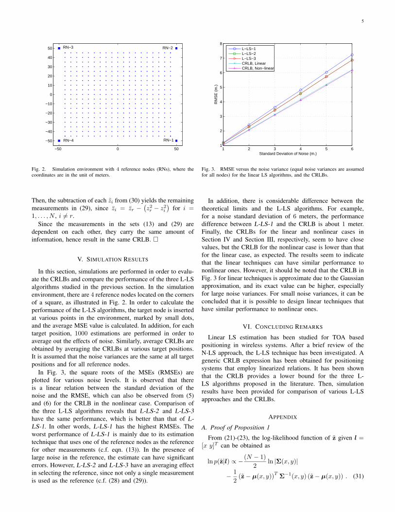
Fig. 2. Simulation environment with 4 reference nodes (RNs), where thecoordinates are in the unit of meters.

Then, the subtraction of each zi from (30) yields the remainingmeasurements in (29), since zi = zr −

(z2r − z2

i

)for i =

1, . . . , N , i 6= r.Since the measurements in the sets (13) and (29) are

dependent on each other, they carry the same amount ofinformation, hence result in the same CRLB. ¤

V. SIMULATION RESULTS

In this section, simulations are performed in order to evalu-ate the CRLBs and compare the performance of the three L-LSalgorithms studied in the previous section. In the simulationenvironment, there are 4 reference nodes located on the cornersof a square, as illustrated in Fig. 2. In order to calculate theperformance of the L-LS algorithms, the target node is insertedat various points in the environment, marked by small dots,and the average MSE value is calculated. In addition, for eachtarget position, 1000 estimations are performed in order toaverage out the effects of noise. Similarly, average CRLBs areobtained by averaging the CRLBs at various target positions.It is assumed that the noise variances are the same at all targetpositions and for all reference nodes.

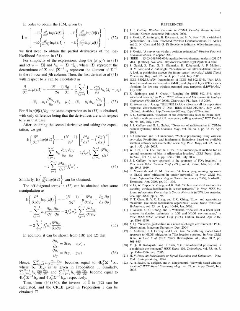
In Fig. 3, the square roots of the MSEs (RMSEs) areplotted for various noise levels. It is observed that thereis a linear relation between the standard deviation of thenoise and the RMSE, which can also be observed from (5)and (6) for the CRLB in the nonlinear case. Comparison ofthe three L-LS algorithms reveals that L-LS-2 and L-LS-3have the same performance, which is better than that of L-LS-1. In other words, L-LS-1 has the highest RMSEs. Theworst performance of L-LS-1 is mainly due to its estimationtechnique that uses one of the reference nodes as the referencefor other measurements (c.f. eqn. (13)). In the presence oflarge noise in the reference, the estimate can have significanterrors. However, L-LS-2 and L-LS-3 have an averaging effectin selecting the reference, since not only a single measurementis used as the reference (c.f. (28) and (29)).

1 2 3 4 5 61

2

3

4

5

6

7

8

Standard Deviation of Noise (m.)

RM

SE

(m

.)

L−LS−1L−LS−2L−LS−3CRLB, LinearCRLB, Non−linear

Fig. 3. RMSE versus the noise variance (equal noise variances are assumedfor all nodes) for the linear LS algorithms, and the CRLBs.

In addition, there is considerable difference between thetheoretical limits and the L-LS algorithms. For example,for a noise standard deviation of 6 meters, the performancedifference between L-LS-1 and the CRLB is about 1 meter.Finally, the CRLBs for the linear and nonlinear cases inSection IV and Section III, respectively, seem to have closevalues, but the CRLB for the nonlinear case is lower than thatfor the linear case, as expected. The results seem to indicatethat the linear techniques can have similar performance tononlinear ones. However, it should be noted that the CRLB inFig. 3 for linear techniques is approximate due to the Gaussianapproximation, and its exact value can be higher, especiallyfor large noise variances. For small noise variances, it can beconcluded that it is possible to design linear techniques thathave similar performance to nonlinear ones.

VI. CONCLUDING REMARKS

Linear LS estimation has been studied for TOA basedpositioning in wireless systems. After a brief review of theN-LS approach, the L-LS technique has been investigated. Ageneric CRLB expression has been obtained for positioningsystems that employ linearized relations. It has been shownthat the CRLB provides a lower bound for the three L-LS algorithms proposed in the literature. Then, simulationresults have been provided for comparison of various L-LSapproaches and the CRLBs.

APPENDIX

A. Proof of Proposition 1

From (21)-(23), the log-likelihood function of z given l =[x y]T can be obtained as

ln p(z|l) ∝ − (N − 1)2

ln |Σ(x, y)|

− 12

(z− µ(x, y))T Σ−1(x, y) (z− µ(x, y)) . (31)

6

In order to obtain the FIM, given by

I =

−E{

∂2

∂x2 lnp(z|l)}

−E{

∂2

∂x∂y lnp(z|l)}

−E{

∂2

∂x∂y lnp(z|l)}

−E{

∂2

∂y2 lnp(z|l)}

, (32)

we first need to obtain the partial derivatives of the log-likelihood function in (31).

For simplicity of the expressions, drop the (x, y)’s in (31)and let g = |Σ| and hij = [Σ−1]ij , where |Σ| represent thedeterminant of Σ and [Σ−1]ij represent the element of Σ−1

in the ith row and jth column. Then, the first derivative of (31)with respect to x can be calculated as

∂

∂xln p(z|l) = − (N − 1)

2g

∂g

∂x− 1

2

N−1∑

i,j=1

{− ∂µi

∂xhij(zj − µj)

+ (zi − µi)∂hij

∂x(zj − µj)− (zi − µi)hi,j

∂µj

∂x

}. (33)

For ∂ ln p(z|l)/∂y, the same expression as in (33) is obtained,with only difference being that the derivatives are with respectto y in that case.

After obtaining the second derivative and taking the expec-tation, we get

E{

∂2

∂x2lnp(z|l)

}= − (N − 1)

2g2

[g∂2g

∂x2−

(∂g

∂x

)2]

−N−1∑

i,j=1

hij∂µi

∂x

∂µj

∂x− 2f2

Nσ2N

N−1∑

i,j=1

∂2hij

∂x2

− 2N−1∑

i=1

∂2hii

∂x2f2

i σ2i . (34)

Similarly, E{

∂2

∂y2 lnp(z|l)}

can be obtained.

The off-diagonal terms in (32) can be obtained after somemanipulation as

E{

∂2

∂x∂ylnp(z|l)

}= − (N − 1)

2g2

[g

∂2g

∂x∂y− ∂g

∂x

∂g

∂y

]

−N−1∑

i,j=1

hij∂µi

∂x

∂µj

∂y− 2f2

Nσ2N

N−1∑

i,j=1

∂2hij

∂x∂y

− 2N−1∑

i=1

f2i σ2

i

∂2hii

∂x∂y. (35)

In addition, it can be shown from (18) and (2) that∂µi

∂x= 2(xi − xN ) ,

∂µi

∂y= 2(yi − yN ) . (36)

Hence,∑N−1

i,j=1 hij∂µi

∂x∂µj

∂x becomes equal to 4bTx Σ−1bx,

where bx (by) is as given in Proposition 1. Similarly,∑N−1i,j=1 hij

∂µi

∂y∂µj

∂y and∑N−1

i,j=1 hij∂µi

∂x∂µj

∂y become equal to4bT

y Σ−1by and 4bTx Σ−1by , respectively.

Then, from (34)-(36), the inverse of I in (32) can becalculated, and the CRLB given in Proposition 1 can beobtained. ¤

REFERENCES

[1] J. J. Caffery, Wireless Location in CDMA Cellular Radio Systems.Boston: Kluwer Academic Publishers, 2000.

[2] S. Gezici, Z. Sahinoglu, H. Kobayashi, and H. V. Poor, “Ultra widebandgeolocation,” in Ultra Wideband Wireless Communications, H. Arslanand Z. N. Chen and M.-G. Di Benedetto (editors), Wiley-Interscience,2006.

[3] S. Gezici, “A survey on wireless position estimation,” Wireless PersonalCommunications, to appear, 2007.

[4] “IEEE 15-03-0489-03-004a-application-requirement-analysis-031127v0.4.” [Online]. Available: http://www.ieee802.org/15/pub/TG4.html

[5] S. Gezici, Z. Tian, G. B. Giannakis, H. Kobayashi, A. F. Molisch,H. V. Poor, and Z. Sahinoglu, “Localization via ultra-wideband radios:A look at positioning aspects for future sensor networks,” IEEE SignalProcessing Mag., vol. 22, no. 4, pp. 70–84, July 2005.

[6] IEEE P802.15.4a/D4 (Amendment of IEEE Std 802.15.4), “Part 15.4:Wireless medium access control (MAC) and physical layer (PHY) spec-ifications for low-rate wireless personal area networks (LRWPANs),”July 2006.

[7] Z. Sahinoglu and S. Gezici, “Ranging for IEEE 802.15.4a ultra-wideband devices,” in Proc. IEEE Wireless and Microwave TechnologyConference (WAMICON 2006), Clearwater, FL, Dec. 4-5 2006.

[8] K. Siwiak and J. Gabig, “IEEE 802.15.4IGa informal call for applicationresponse, contribution#11,” Doc.: IEEE 802.15-04/266r0, July, 2003.[Online]. Available: http://www.ieee802.org/15/pub/TG4a.html

[9] F. C. Commission, “Revision of the commissions rules to insure com-patibility with enhanced 911 emergency calling systems,” FCC DocketNo. 94-102, July, 1996.

[10] J. J. Caffery and G. L. Stuber, “Overview of radiolocation in CDMAcellular systems,” IEEE Commun. Mag., vol. 36, no. 4, pp. 38–45, Apr.1998.

[11] F. Gustafsson and F. Gunnarsson, “Mobile positioning using wirelessnetworks: Possibilites and fundamental limitations based on availablewireless network measurements,” IEEE Sig. Proc. Mag., vol. 22, no. 4,pp. 41–53, July 2005.

[12] W. Kim, J. G. Lee, and G. I. Jee, “The interior-point method for anoptimal treatment of bias in trilateration location,” IEEE Trans. Vehic.Technol., vol. 55, no. 4, pp. 1291–1301, July 2006.

[13] J. J. Caffery, “A new approach to the geometry of TOA location,” inProc. IEEE Vehic. Technol. Conf. (VTC), vol. 4, Boston, MA, Sep. 2000,pp. 1943–1949.

[14] S. Venkatesh and R. M. Buehrer, “A linear programming approachto NLOS error mitigation in sensor networks,” in Proc. IEEE Int.Symp. Information Processing in Sensor Networks (IPSN), Nashville,Tennessee, Apr. 2006, pp. 301–308.

[15] Z. Li, W. Trappe, Y. Zhang, and B. Nath, “Robust statistical methods forsecuring wireless localization in sensor networks,” in Proc. IEEE Int.Symp. Information Processing in Sensor Networks (IPSN), Los Angeles,CA, Apr. 2005, pp. 91–98.

[16] Y. T. Chan, H. Y. C. Hang, and P. C. Ching, “Exact and approximatemaximum likelihood localization algorithms,” IEEE Trans. VehicularTechnology, vol. 55, no. 1, pp. 10–16, Jan. 2006.

[17] I. Guvenc, C. C. Chong, and F. Watanabe, “Analysis of a linear least-squares localization technique in LOS and NLOS environments,” inProc. IEEE Vehic. Technol. Conf. (VTC), Dublin, Ireland, Apr. 2007,pp. 1886–1890.

[18] Y. Qi, “Wireless geolocation in a non-line-of-sight environment,” Ph.D.Dissertation, Princeton University, Dec. 2004.

[19] S. Al-Jazzar, J. J. Caffery, and H.-R. You, “A scattering model basedapproach to NLOS mitigation in TOA location systems,” in Proc. IEEEVehic. Technol. Conf. (VTC 2002), Birmingham, AL, May 2002, pp.861–865.

[20] Y. Qi, H. Kobayashi, and H. Suda, “On time-of-arrival positioning ina multipath environment,” IEEE Trans. Veh. Technology, vol. 55, no. 5,pp. 1516–1526, Sep. 2006.

[21] H. V. Poor, An Introduction to Signal Detection and Estimation. NewYork: Springer-Verlag, 1994.

[22] A. H. Sayed, A. Tarighat, and N. Khajehnouri, “Network-based wirelesslocation,” IEEE Signal Processing Mag., vol. 22, no. 4, pp. 24–40, July2005.