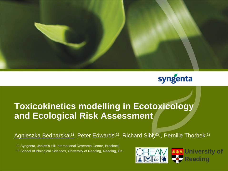
Agnieszka Bednarska(1), Peter Edwards(1), Richard Sibly(2), Pernille Thorbek(1)

Toxicokinetics modelling in Ecotoxicology and Ecological Risk Assessment

(1) Syngenta, Jealott’s Hill International Research Centre, Bracknell(2) School of Biological Sciences, University of Reading, Reading, UK University of

Reading

2

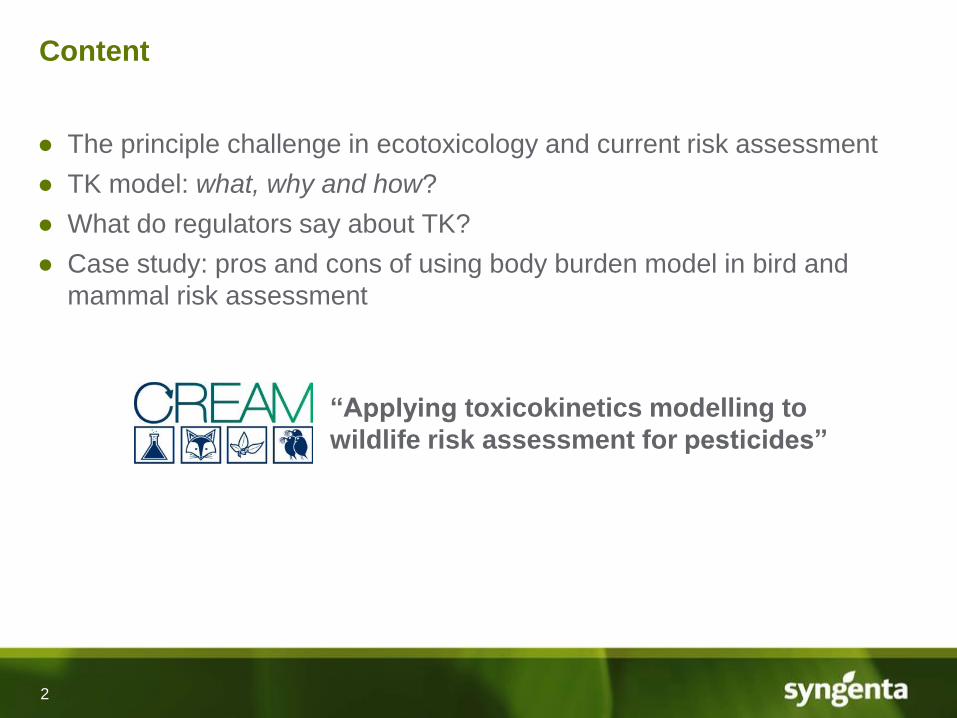
Content

● The principle challenge in ecotoxicology and current risk assessment

● TK model: what, why and how?

● What do regulators say about TK?

● Case study: pros and cons of using body burden model in bird and

mammal risk assessment

“Applying toxicokinetics modelling to

wildlife risk assessment for pesticides”

3

Background

● How to accurately characterize the risk of chemicals to a diversity of

species with different behaviours and sensitivities from a limited amount

of information?

● The current risk assessment

• Based on external exposure measurements

• Do not represent field exposure

● TK model

• Absorption, Distribution, Metabolism, Excretion (ADME)

4

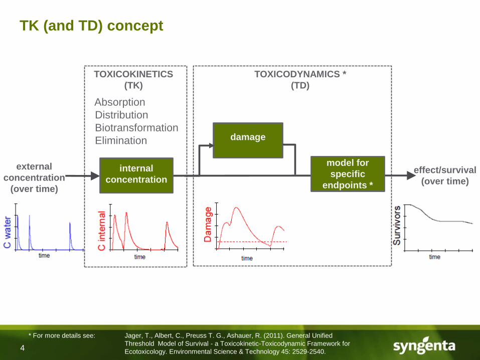
TK (and TD) concept

external

concentration

(over time)

effect/survival

(over time)

damage

TOXICODYNAMICS *

(TD)

* For more details see: Jager, T., Albert, C., Preuss T. G., Ashauer, R. (2011). General Unified

Threshold Model of Survival - a Toxicokinetic-Toxicodynamic Framework for

Ecotoxicology. Environmental Science & Technology 45: 2529-2540.

internal

concentration

TOXICOKINETICS

(TK)

Absorption

Distribution

Biotransformation

Elimination

model for

specific

endpoints *

5

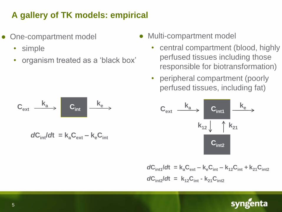
A gallery of TK models: empirical

● One-compartment model

• simple

• organism treated as a ‘black box’

dCint/dt = kaCext – keCint

ka keCintCextka keCint1Cext

Cint2

k12 k21

dCint1/dt = kaCext – keCint – k12Cint + k21Cint2

dCint2/dt = k12Cint - k21Cint2

● Multi-compartment model

• central compartment (blood, highly

perfused tissues including those

responsible for biotransformation)

• peripheral compartment (poorly

perfused tissues, including fat)

6

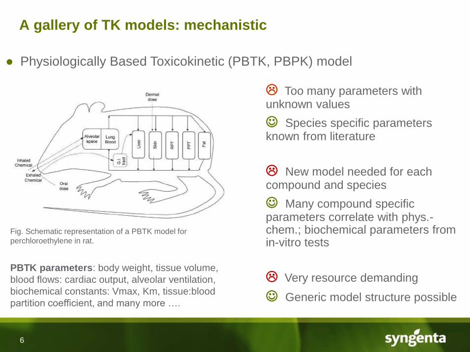
● Physiologically Based Toxicokinetic (PBTK, PBPK) model

A gallery of TK models: mechanistic

Too many parameters with unknown values

Species specific parameters known from literature

New model needed for each compound and species

Many compound specific parameters correlate with phys.-chem.; biochemical parameters from in-vitro tests

Very resource demanding

Generic model structure possible

Fig. Schematic representation of a PBTK model for

perchloroethylene in rat.

PBTK parameters: body weight, tissue volume,

blood flows: cardiac output, alveolar ventilation,

biochemical constants: Vmax, Km, tissue:blood

partition coefficient, and many more ….

7

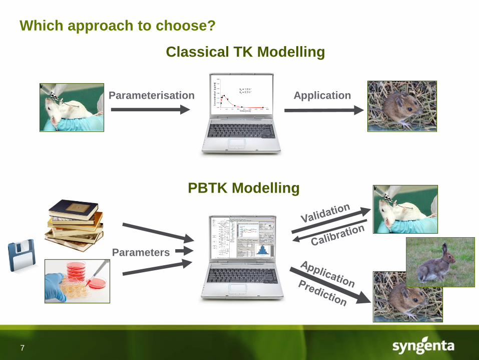
Which approach to choose?

Parameterisation Application

MODEL

Parameters

Classical TK Modelling

PBTK Modelling

8

Aim of the project

Develop TK model to be used in bird and mammal risk assessment

● Simple enough to be manageable and applicable across a range of exposure

scenarios (and species)

● Sufficiently complex for representing all crucial processes

● Parameterisation methods using standard regulatory data

(no additional tests required)

9

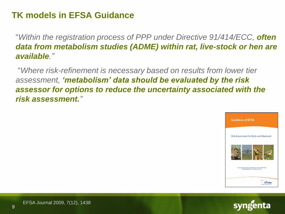
TK models in EFSA Guidance

“Within the registration process of PPP under Directive 91/414/ECC, often

data from metabolism studies (ADME) within rat, live-stock or hen are

available.”

“Where risk-refinement is necessary based on results from lower tier

assessment, ‘metabolism’ data should be evaluated by the risk

assessor for options to reduce the uncertainty associated with the

risk assessment.”

EFSA Journal 2009, 7(12), 1438

10

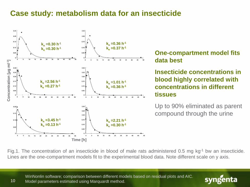
Case study: metabolism data for an insecticide

Fig.1. The concentration of an insecticide in blood of male rats administered 0.5 mg kg-1 bw an insecticide.

Lines are the one-compartment models fit to the experimental blood data. Note different scale on y axis.

One-compartment model fits

data best

Insecticide concentrations in

blood highly correlated with

concentrations in different

tissues

Up to 90% eliminated as parent

compound through the urine

WinNonlin software; comparison between different models based on residual plots and AIC.

Model parameters estimated using Marquardt method.

ka =0.30 h-1

ke =0.30 h-1

ka =2.56 h-1

ke =0.27 h-1

ka =3.45 h-1

ke =0.13 h-1

ka =0.36 h-1

ke =0.37 h-1

ka =1.01 h-1

ke =0.36 h-1

ka =2.21 h-1

ke =0.30 h-1

Co

nc

en

tra

tio

n [

µg

ml-1

]

Time [h]

11

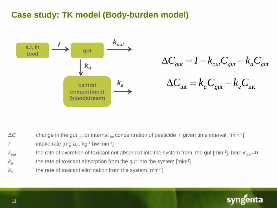
Case study: TK model (Body-burden model)

intint CkCkC eguta

ΔC change in the gut gut or internal int concentration of pesticide in given time interval, [min-1]

I intake rate [mg a.i. kg-1 bw min-1]

kout the rate of excretion of toxicant not absorbed into the system from the gut [min-1], here kout =0

ka the rate of toxicant absorption from the gut into the system [min-1]

ke the rate of toxicant elimination from the system [min-1]

a.i. in

foodgut

central

compartment

(bloodstream)

ka

ke

koutI

gutagutoutgut CkCkIC

12

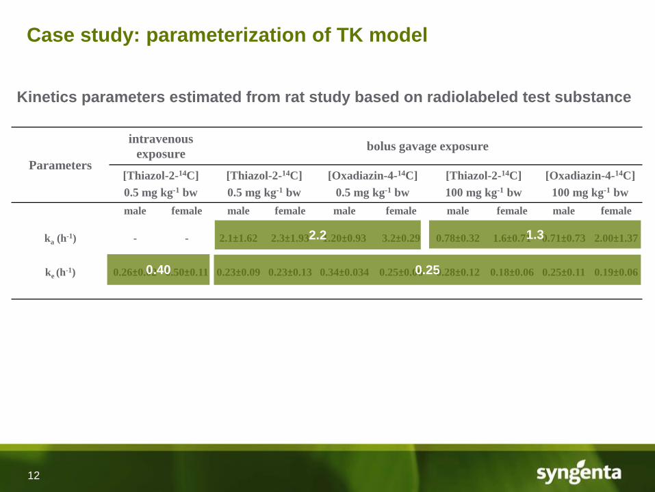
Case study: parameterization of TK model

Parameters

intravenous

exposurebolus gavage exposure

[Thiazol-2-14C]

0.5 mg kg-1 bw

[Thiazol-2-14C]

0.5 mg kg-1 bw

[Oxadiazin-4-14C]

0.5 mg kg-1 bw

[Thiazol-2-14C]

100 mg kg-1 bw

[Oxadiazin-4-14C]

100 mg kg-1 bw

male female male female male female male female male female

ka (h-1) - - 2.1±1.62 2.3±1.93 1.20±0.93 3.2±0.29 0.78±0.32 1.6±0.71 0.71±0.73 2.00±1.37

ke (h-1) 0.26±0.02 0.50±0.11 0.23±0.09 0.23±0.13 0.34±0.034 0.25±0.06 0.28±0.12 0.18±0.06 0.25±0.11 0.19±0.06

Kinetics parameters estimated from rat study based on radiolabeled test substance

2.2 1.3

0.40 0.25

13

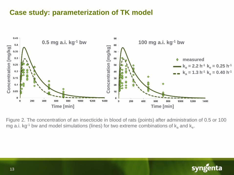
Case study: parameterization of TK model C

on

ce

ntr

ati

on

[m

g/k

g]

measured

ka = 2.2 h-1 ke = 0.25 h-1

ka = 1.3 h-1 ke = 0.40 h-1

0.5 mg a.i. kg-1 bw 100 mg a.i. kg-1 bw

Co

nc

en

tra

tio

n [

mg

/kg

]Time [min]

Figure 2. The concentration of an insecticide in blood of rats (points) after administration of 0.5 or 100

mg a.i. kg-1 bw and model simulations (lines) for two extreme combinations of ka and ke.

Time [min]

14

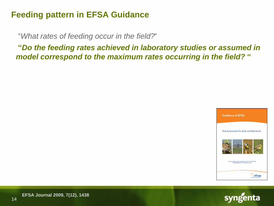
Feeding pattern in EFSA Guidance

EFSA Journal 2009, 7(12), 1438

“What rates of feeding occur in the field?“

“Do the feeding rates achieved in laboratory studies or assumed in

model correspond to the maximum rates occurring in the field? “

15

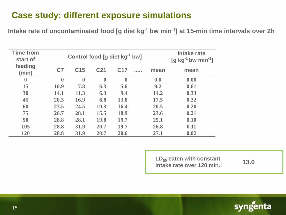
Case study: different exposure simulations

Time from

start of

feeding

(min)

Control food [g diet kg-1 bw]Intake rate

[g kg-1 bw min-1]

Intake rate of LD50

[mg a.i. kg-1 bw min-1]

C7 C15 C21 C17 ..... mean mean mean

0 0 0 0 0 0.0 0.00 0.0

15 10.9 7.8 6.3 5.6 9.2 0.61 35.3

30 14.1 11.3 6.3 9.4 14.2 0.33 19.1

45 20.3 16.9 6.8 13.8 17.5 0.22 12.7

60 23.5 24.5 10.3 16.4 20.5 0.20 11.6

75 26.7 28.1 15.5 18.9 23.6 0.21 12.2

90 28.8 28.1 19.8 19.7 25.1 0.10 5.8

105 28.8 31.9 20.7 19.7 26.8 0.11 6.4

120 28.8 31.9 20.7 20.6 27.1 0.02 1.2

Intake rate of uncontaminated food [g diet kg-1 bw min-1] at 15-min time intervals over 2h

LD50 eaten with constant

intake rate over 120 min.:13.0

16

Time [min]

Co

ncen

trati

on

[m

g k

g-1

bw

]

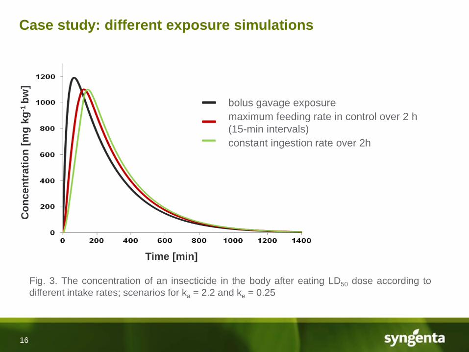
Fig. 3. The concentration of an insecticide in the body after eating LD50 dose according to

different intake rates; scenarios for ka = 2.2 and ke = 0.25

bolus gavage exposure

maximum feeding rate in control over 2 h

(15-min intervals)

constant ingestion rate over 2h

Case study: different exposure simulations

17

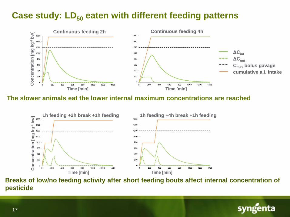
Case study: LD50 eaten with different feeding patterns

Breaks of low/no feeding activity after short feeding bouts affect internal concentration of

pesticide

Co

ncen

trati

on

[m

g k

g-1

bw

]

Time [min]

ΔCint

ΔCgut

Cmax bolus gavage

cumulative a.i. intake

Continuous feeding 2h

Time [min] Time [min]

1h feeding +2h break +1h feeding 1h feeding +4h break +1h feeding

Co

nc

en

tra

tio

n [

mg

kg

-1b

w]

Continuous feeding 4h

Time [min]

The slower animals eat the lower internal maximum concentrations are reached

18

● TK models are considered as a refinment tool for risk assessment in EU

guidance for birds and mammals

● ADME data can be used to parameterize a body burden (or other TK) model

● Key assumptions which should be checked before using BB approaches:

• Can kinetics be described as a first order process or is it more complex?

• How many compartments should be included in the model?

• Is it necessary to represent target organ(s) as separate compartment(s) or

is the toxicant concentration in systemic circulation (blood) sufficient?

● BB model based on total radioactivity, so metabolites are not characterized

separately - PBTK models may be sometimes preferred

● Behavioural responses may moderate exposure - taking into account

behavioural responses, timescales of exposure and kinetics improve risk

assessment

Conclusions

19

Thank you for your attention

This research has been financially supported by the European

Union under the 7th Framework Programme (project acronym

CREAM, contract number PITN-GA-2009-238148)

Everything should be made as simple as possible, but not simpler.

- Albert Einstein

● Choice between approaches (model structure and type) depends on intended

use – make model only as complex as needed

Conclusions