Embed Size (px)
Citation preview
Politecnico di MilanoDipartimento di Elettronica, Informazione e Bioingegneria
Dottorato di Ricerca in Ingegneria dell’Informazione
Towards the Definition of aMethodology for the Design ofTunable Dependable Systems
Doctoral Dissertation of:Matteo Carminati
Advisor:Prof. Cristiana Bolchini
Tutor:Prof. Donatella Sciuto
Supervisor of the Doctoral Program:Prof. Carlo Fiorini
2014 – XXVII

Politecnico di MilanoDipartimento di Elettronica, Informazione e Bioingegneria
Piazza Leonardo da Vinci, 32 I-20133 — Milano


Abstract
The problem of guaranteeing the correct behavior in digital systems evenwhen faults occur has been investigated for several years. However, theresearchers’ efforts have been mainly devoted to safety- and mission-critical systems, where the occurrence of faults (both transient and per-manent) can be extremely hazardous. Nowadays, the need to providereliability also for non-critical application environments is gaining a lotof momentum, due to the pervasiveness of embedded systems and theirincreasing susceptibility due to technology scaling. While in critical ap-plications the budget devoted to reliability is almost unlimited and itis not to be compromised, in non-critical scenarios the limited availablebudget used to guarantee the best performance and energy consumptionis to be shared for providing reliability as well.In the past, great effort has been devoted to provide strict reliability
management. This led to the shared belief that reliability is to be con-sidered from the early stages of the embedded systems design process.In fact, as this process is becoming more and more complex, approachesthat do not consider reliability throughout all the design steps may leadto expensive or not-optimized solutions. Moreover, considering reliabil-ity in a holistic way allows to drive the several decisions by exploiting thesynergy of both the most classical aspects and reliability-oriented ones.Postponing the reliability assessment to the later phases of the designflow on a system prototype is not appealing, because failure in achiev-ing the desired level of reliability would be detected too late. However,the complexity of managing reliability, performance and power/energyconsumption all at the same time grows exponentially, especially whenseveral decision variables are available in the considered system. Forthis reason it is not possible to envision a system able to properly reactto any possible scenario on the basis of decisions precomputed at de-sign time; a new paradigm based on self-adaptability is to be designed.Self-adaptive systems are becoming quite common when dealing withsuch complex systems: relevant examples are available in literature ifperformance management is considered.Given these motivations, we argue that the self-adaptive paradigm is
to be implemented when designing embedded systems with the aim ofconsidering reliability as a driving dimension. In particular, in this thesis
5

we propose a comprehensive management framework for dealing with re-liability in multi/manycore embedded systems. Reliability is consideredboth for permanent/transient faults management and components agingmitigation. This framework implements a well-known control loop wherethe status of the system and the environment are sensed (observe), adap-tation is defined through decisions made at runtime to meet the specifiedgoals and constraints (decide), and the values of the system parametersare modified accordingly (act). The designed framework is integratedin a two-layer heterogeneous multi/manycore architecture which is con-sidered as the reference hardware platform. Self-adaptability is enabledthrough independent control layers implemented on top of the referencearchitecture. At the top-level, the manycore one, a control cycle en-sures the combined optimization of the overall architecture lifetime andof the energy consumption due to communication among nodes. On theother hand, within each node, two control cycles have been designed: onefor dealing with faults occurrence (through the selection of the properscheduling technique) and another one for mitigating components agingand minimizing energy consumption (thanks to smart mapping algo-rithms). Moreover, in the considered optimization process, performanceis always considered as a constraint, in the form of applications deadlines,in order to guarantee a satisfying quality of service.In addition to the above contributions, two more ones deserve to be
considered. First, the definition of a model to describe and classify self-adaptive computing systems on the basis of their driving dimensions(goals and constraints), the available measures and acting parameters.Second, a tool for estimating the reliability function and the expectedlifetime of complex multi/manycore architectures, able to tolerate mul-tiple failures and considering varying workloads.
6

Sommario
Il problema di garantire il corretto funzionamento dei sistemi digitali è damolti anni oggetto di ricerca accademica. Tuttavia, gli sforzi dei ricerca-tori si sono concentrati soprattutto su sistemi il cui fallimento causa graviripercussioni sulla salute delle persone o sulla buona riuscita di progettiparticolarmente onerosi. Al giorno d’oggi, invece, sta diventando semprepiù importante la necessità di rendere affidabili anche quei sistemi chenon possono essere definiti critici, ma che hanno raggiunto una grandediffusione e risultano sempre più proni alla rottura a causa delle ridottedimensioni dei loro componenti. Mentre in scenari critici le risorse allo-cate per far fronte a problemi di affidabilità sono pressochè illimitate enon si deve scendere a compromessi, in scenari che non presentano crit-icità le risorse a disposizione sono limitate e devono essere sfruttate perottimizzare il funzionamento del dispositivo stesso, anche in termini diprestazioni ed energia consumata.Le ricerche svolte in passato hanno portato alla luce la necessità di con-
siderare i requisiti di affidabilità del sistema sin dal principio del processodi progettazione. Infatti, a causa della sempre crescente complessità diquesto processo, approcci che non considerano il livello di affidabilitàrichiesto in tutti i passi di progettazione rischiano di portare a soluzionieccessivamente costose e/o non ottimizzate. Considerare, invece, gli as-petti di affidabilità come parte integrante di tutto il processo di pro-gettazione permette trarre giovamento sia da tecniche classiche che datecniche esplicitamente orientate all’affidabilità. Postporre la verifica dellivello di affidabilità raggiunto al termine del processo di prototipazionenon è invece una pratica saggia, poichè, in caso di fallimento, può causarela perdita di tempo e denaro. Questa necessità di integrazione causa peròun aumento della complessità di progetto, in particolar modo quando iparametri su cui è possibile agire sono molti. Per questo motivo non èpensabile un sistema capace di reagire correttamente ad ogni possibilesituazione sulla base di decisione pre-calcolate; è necessario adottare unparadigma di progettazione che preveda l’auto adattamento del sistemaa tempo di esecuzione. I sistemi auto-adattativi per la gestione di sis-temi complessi stanno infatti diventando sempre più comuni, soprattuttonell’ambito dell’ottimizzazione delle prestazioni.Sulla base di queste motivazioni, sosteniamo che il paradigma di pro-
7

gettazione basato su auto-adattatività debba essere impiegato anchequando si ha a che fare con sistemi embedded che richiedano un de-terminato livello di affidabilità. In particolare, in questa tesi si proponeun’infrastruttura completa per la gestione dell’affidabilità in sistemi em-bedded composti da multi/manycore. L’affidabilità viene considerata siain termini di gestione dei guasti (sia transitori che permanenti) sia comemitigazione dell’invecchiamento dei componenti. L’infrastruttura pro-posta realizza un ciclo di controllo proposto in letteratura e compostoda tre fasi fondamentali: l’osservazione dello stato interno del sistemae dell’ambiente in cui vive (osserva), l’adattamento attraverso decisioniprese a tempo di esecuzione per rispettare i vincoli e gli obiettivi prece-dentemente specificati (decidi) e l’attuazione delle decisioni prese at-traverso la modifica dei parametri del sistema (agisci). L’infrastrutturaè stata progettata in modo da integrarsi all’interno dell’architetturadi riferimento, composta da due livelli: ad un livello più alto una pi-attaforma manycore, in cui ogni nodo, a livello più basso, è compostoda un sistema multicore. Il sistema è reso auto-adattativo tramite larealizzazione di cicli di controllo indipendenti che lavorano ai diversi liv-elli di astrazione. Ad alto livello, un primo ciclo di controllo garantiscel’ottimizzazione congiunta dell’invecchiamento dei nodi e del consumodi energia dovuto alla comunicazione tra gli stessi. All’interno di ogninodo sono stati realizzati altri due cicli di controllo: il primo si occupadi gestire le occorrenze di guasti (attraverso la selezione della tecnicadi scheduling più adatta tra quelle disponibili), mentre il secondo di bi-lanciare l’invecchiamento dei componenti e di minimizzare l’energia con-sumata (grazie ad algoritmi di mapping intelligenti). Nel corso di questoprocesso di ottimizzazione, le prestazioni del sistema vengono sempreconsiderate come un vincolo da rispettare, nella forma di deadline tem-porali, in modo tale che il sistema garantisca sempre una soddisfacentequalità del servizio erogato.Altri due contributi di questa tesi meritano di essere citati, a comple-
mento di quelli già descritti in precedenza. In primo luogo, la definizionedi un modello per descrivere e classificare i sistemi auto-adattativi sullabase delle dimensioni che guidano il loro adattamento, dei dati disponi-bili e dei parametri sui quali è possibili agire. In secondo luogo, uno stru-mento per stimare l’affidabilità e il tempo di vista atteso di un’architetturacomplessa come quella di riferimento, sottoposta a carichi di lavoro vari-abili nel tempo e capace di tollerare la rottura di alcuni suoi componenti.
8

Contents
1 Introduction 171.1 Thesis Statement . . . . . . . . . . . . . . . . . . . . . . . 191.2 Overview of Research . . . . . . . . . . . . . . . . . . . . . 201.3 Contributions . . . . . . . . . . . . . . . . . . . . . . . . . 221.4 Publications . . . . . . . . . . . . . . . . . . . . . . . . . . 241.5 Thesis Organization . . . . . . . . . . . . . . . . . . . . . 25
2 Background & Preliminaries 272.1 Background . . . . . . . . . . . . . . . . . . . . . . . . . . 27
2.1.1 Multi/Manycore Systems . . . . . . . . . . . . . . 272.1.2 Dependable Systems . . . . . . . . . . . . . . . . . 322.1.3 Self-Adaptive Systems . . . . . . . . . . . . . . . . 35
2.2 Working Scenario . . . . . . . . . . . . . . . . . . . . . . . 372.2.1 Reference Platform . . . . . . . . . . . . . . . . . . 382.2.2 Baseline . . . . . . . . . . . . . . . . . . . . . . . . 392.2.3 Key Performance Indicators . . . . . . . . . . . . . 402.2.4 Case Study . . . . . . . . . . . . . . . . . . . . . . 41
3 Self-Adaptive Systems Design 433.1 Orchestrator . . . . . . . . . . . . . . . . . . . . . . . . . . 43
3.1.1 Monitoring Infrastructure . . . . . . . . . . . . . . 443.1.2 Decision Policies . . . . . . . . . . . . . . . . . . . 463.1.3 Actuating Elements . . . . . . . . . . . . . . . . . 47
3.2 A Model for Self-Adaptive Computing Systems . . . . . . 473.2.1 The Context Concept . . . . . . . . . . . . . . . . 503.2.2 Formalization . . . . . . . . . . . . . . . . . . . . . 553.2.3 Validation . . . . . . . . . . . . . . . . . . . . . . . 57
3.3 Final Remarks . . . . . . . . . . . . . . . . . . . . . . . . 60
4 Runtime Transient Fault Management 614.1 Background . . . . . . . . . . . . . . . . . . . . . . . . . . 614.2 State of the Art . . . . . . . . . . . . . . . . . . . . . . . . 624.3 Fault Tolerance through Self-Adaptiveness . . . . . . . . . 64
4.3.1 Fault Management Mechanisms . . . . . . . . . . . 654.3.2 Layer Internals . . . . . . . . . . . . . . . . . . . . 67
9
Contents
4.3.3 Orchestrator Design . . . . . . . . . . . . . . . . . 684.4 Experimental Results . . . . . . . . . . . . . . . . . . . . . 76
4.4.1 Experimental Set-up . . . . . . . . . . . . . . . . . 774.4.2 First Experimental Session . . . . . . . . . . . . . 784.4.3 Second Experimental Session . . . . . . . . . . . . 81
4.5 Final Remarks . . . . . . . . . . . . . . . . . . . . . . . . 84
5 Runtime Aging Management 875.1 Background . . . . . . . . . . . . . . . . . . . . . . . . . . 875.2 Aging Evaluation . . . . . . . . . . . . . . . . . . . . . . . 91
5.2.1 State of the Art . . . . . . . . . . . . . . . . . . . . 915.2.2 The proposed framework . . . . . . . . . . . . . . . 925.2.3 Experimental evaluation . . . . . . . . . . . . . . . 97
5.3 Aging Mitigation through Self-Adaptiveness . . . . . . . . 1045.3.1 Single Node . . . . . . . . . . . . . . . . . . . . . . 1075.3.2 Multi Node and Computation Energy . . . . . . . 1155.3.3 Multi Node and Communication Energy . . . . . . 1185.3.4 Putting it all together . . . . . . . . . . . . . . . . 128
5.4 Final Remarks . . . . . . . . . . . . . . . . . . . . . . . . 131
6 Conclusions & Future Works 133
10

List of Figures
1.1 A graphical overview of the proposed system composition. 21
2.1 Representation of the defined architectural concepts. . . . 282.2 A simple application represented by a task-graph. . . . . . 312.3 The Observe-Decide-Act (ODA) control loop. . . . . . . . 362.4 Graphical representation of the reference platform. . . . . 39
3.1 Overview of the proposed framework. . . . . . . . . . . . . 453.2 Graphical representation of the context meta-model; each
rectangle represents a context dimension, those with roundedcorners are the driving dimensions. Dotted rectangles in-dicate dimensions that might not exist in some contexts.Segments represent relations among dimensions. . . . . . . 54
3.3 Context meta-model and dimension domains for self-adaptivecomputing systems. . . . . . . . . . . . . . . . . . . . . . . 54
3.4 Context dimensions and domains for METE research project. 593.5 Context dimensions and domains for Into The Wild project. 593.6 Context dimensions and domains for Metronome project. . 60
4.1 Context dimensions and domains for the fault tolerancemanagement self-adaptive system. . . . . . . . . . . . . . . 61
4.2 System structure overview: the FM layer acts between theapplications and the OS. . . . . . . . . . . . . . . . . . . . 64
4.3 Duplication with Comparison (DWC) technique appliedto all the tasks of the sample application of Figure 2.2. . . 65
4.4 Triplication (TMR) technique applied to all the tasks ofthe sample application of Figure 2.2. . . . . . . . . . . . . 66
4.5 Duplication with Comparison and Re-execution (DWCR)technique applied to all the tasks of the sample applicationof Figure 2.2. . . . . . . . . . . . . . . . . . . . . . . . . . 67
4.6 The Observe–Decide–Act control loop. . . . . . . . . . . . 684.7 Application’s task–graph hardened at the two different
levels of granularity: the colored dashed tasks representthe voter nodes added to make fault mitigation possible. . 71
11

List of Figures
4.8 If PE0 is permanently faulty, the presented mapping ofthe tasks on three processing cores, PE0, PE1 and PE2,causes TMR to fail. . . . . . . . . . . . . . . . . . . . . . . 72
4.9 A FSM representation of the decision process in the casereliability is the constrained dimension. . . . . . . . . . . . 75
4.10 Task-graph for the edge detector application. . . . . . . . 784.11 Overall execution times for the edge detector on the vari-
ous architectures stimulated by each fault list. . . . . . . . 804.12 Metrics computed over the overall experiment execution. . 824.13 Throughput for the edge detector on the architecture with
12 processing cores, stimulated with a fault list presentinga variable failure rate and a permanent fault. . . . . . . . 84
5.1 Model of a PE’s temperature profile over time. . . . . . . 885.2 Reliability curve considering temperature changes. . . . . 895.3 Workflow of the proposed framework. . . . . . . . . . . . . 935.4 Example of application execution and thermal profile. . . 955.5 Simulations execution times w.r.t. number of failures k. . 1025.6 Iterations number w.r.t. different architectures topologies. 1025.7 Coefficient of variation w.r.t. number of failures k. . . . . 1025.8 Comparison vs. past works for constant workloads. . . . . 1035.9 Reliability curve for different workload change’s periods. . 1055.10 Context dimensions and domains for the aging mitigation
self-adaptive system. . . . . . . . . . . . . . . . . . . . . . 1055.11 Energy consumption vs. lifetime optimization. . . . . . . . 1075.12 Block diagram for the reference energy optimization frame-
work. . . . . . . . . . . . . . . . . . . . . . . . . . . . . . . 1105.13 Block diagram for the proposed lifetime and energy opti-
mization framework. . . . . . . . . . . . . . . . . . . . . . 1105.14 Extension of the proposed framework to a mult-node ar-
chitecture. . . . . . . . . . . . . . . . . . . . . . . . . . . . 1105.15 The proposed approach compared with the baseline frame-
work in a single node architecture. . . . . . . . . . . . . . 1155.16 Control flow chart for the dispatching algorithm. . . . . . 1165.17 The proposed approach compared with the baseline frame-
work in a multi-node architecture. . . . . . . . . . . . . . . 1185.18 Overview of the proposed methodology. . . . . . . . . . . 1225.19 MTTF performance of the proposed approach. . . . . . . 1265.20 MTTF performance with multi-application and multi-throughput
scenarios. . . . . . . . . . . . . . . . . . . . . . . . . . . . 1285.21 Communication energy performance for the proposed tech-
nique. . . . . . . . . . . . . . . . . . . . . . . . . . . . . . 129
12

List of Figures
5.22 Overview of the proposed approach when both communi-cation and computation energy consumptions are optimized.131
6.1 A graphical representation of the research contribution ofthis thesis, organized in self-adaptive layers. . . . . . . . . 134
13


List of Tables
2.1 Baseline summary. . . . . . . . . . . . . . . . . . . . . . . 40
3.1 Model constraints for the METE self-adaptive system. . . 58
4.1 Qualitative performance comparison between TMR andDCR techniques. The comparison refers to the same levelof granularity. . . . . . . . . . . . . . . . . . . . . . . . . . 70
4.2 Qualitative evaluation of the described techniques withreference to reliability aspects (FD: Fault Detection – FT:Fault Tolerance). . . . . . . . . . . . . . . . . . . . . . . . 73
4.3 Execution times for voting and checking various amountof data. . . . . . . . . . . . . . . . . . . . . . . . . . . . . 77
5.1 Comparison of the state the art frameworks (Architecture:single core (S), multicore (M) – Aging Models: exponentialdistribution (E), Weibull distribution (W) – Workload :average temperature (Avg T), average aging factor (Avgα) during the considered period). . . . . . . . . . . . . . . 92
5.2 Energy performance of the proposed dynamic approachwith MTTF optimization only . . . . . . . . . . . . . . . . 127
5.3 Parameters for multi-application and multi-throughput . . 127
15


1 Introduction
The trend of building new complex systems by integrating low-cost, in-herently unreliable Commercial Off-The-Shelf (COTS) components isone of today’s challenges in the design, analysis and development ofmodern computing systems [55]. In fact, the last decade has seen thecomplexity of electronic systems grow faster and faster, because of thedecrease of the components’ size and cost. However, this harsh technol-ogy scaling has led to an increase of the susceptability to both permanentand transient faults due to the variations in the manufacturing processand to the exposition of devices to radiations and noise fluctuations [55].More precisely, the aggressive CMOS scaling exploited to boost computa-tional power, generates higher temperatures, causing physical wear-outphenomena that increase the probability for permanent faults due tocomponents aging to appear. This susceptability is further exacerbatedwhen considering systems constituted by several computational units (toachieve high performance) because of the additional environmental in-teractions between the hardware and the software of the different units.A permanent fault, also known as hard fault, indicates the permanent
going out of commission of a component; on the other hand, a tran-sient fault, or soft fault, does not damage a component permanently,but causes glitches in the elaboration, randomly corrupting either thecomputed data or the control flow being executed, thus jeopardizing theoutput results [61]. Radiations are among the main causes of transientfaults [40]; they are particularly frequent in space, but are becoming anissue also at ground level [77]. Permanent faults are, instead, closelyrelated to devices usage and wear-out phenomena, which are strictlydependent on temperature, operating frequency, voltage and current-density.All these considerations, particularly hazardous in safety- and mission-
critical systems (such as automotive devices and controls, railways, aero-space systems and plant control systems), seriously affect ordinary de-vices as well, when considering the embedded system’s pervasiveness intoday’s life (consumer electronics and home appliances) [100]. There-fore, reliability is increasingly adopted as one of the main optimizationgoals, together with performance and energy optimization, and it needsto be taken into account from the initial phases of the design process.
17

1 Introduction
In non-critical environments, where the available budget to be spentfor reliability is limited, it must be leveraged in order not to introducetoo high costs and/or stringent requirements. This scenario is furthercomplicated by the current shift towards parallel architectures, such asmulticores and manycores. In the last years indeed, a lot of attention hasbeen devoted to the design of architectures integrating multiple cores ona single die, to benefit from the relatively low cost of the computationalpower, while offering high performance through the parallel execution ofdifferent applications [14]. The number of computing resources and theirpower/performance profiles characterize the overall architecture, thatcan be classified as multicore (several units) or manycore (several tens ofunits), and homogeneous (all identical units) or heterogeneous (units withdifferent profiles). However, this opportunity increases the difficulty ofmanaging the available resources, considering the complexity of selectingthe most appropriate resource mixture where to run the workload, andthe fact that, even when homogenous in terms of power/performance,each resource will have its own history, making it heterogeneous fromother points of view (e.g. aging and wear-out levels).
Another level of complexity is introduced by the high dynamism of theworking scenario the considered systems live in. In particoular: i) op-timization goals may vary at runtime (performance, energy consump-tion, reliability), ii) the workload may not be known in advance, andiii) permanent and transient faults may occur, dynamically affecting thebehavior of the system.
As mentioned, in many scenarios the need for reliability may changeduring the system’s activity, depending on the specific working scenario,or it cannot be foreseen at design-time due to the unpredictability of theenvironment. Moreover, knobs allowing the runtime configuration of thecores’ working conditions (as for instance, dynamic voltage/frequencyscaling – DVFS) are usually available. For these reasons, a new wayto dynamically tune the reliability management based on the workingscenario is needed, taking into consideration the incidence of both per-manent and transient faults. The challenge in identifying a suitablesolution for this problem is given by the need for finding a satisfyingtrade-off between benefits and costs at runtime. Since the overall relia-bility problem is not new, although becoming more and more relevant,literature offers a wide set of reliability-oriented approaches; however,most of them tackle the problem of permanent and transient faults sin-gularly or do not take into consideration the possibility for the systemrequirements to vary at runtime, thus needing the initial solution to berecomputed.
18

1.1 Thesis Statement
1.1 Thesis Statement
The previous discussion highlighted the necessity for a new paradigmto be employed in embedded system design, where reliability is to beconsidered as a leading dimension of the design process from its earlystages. It would be unfeasible for the designer to manually evaluateall the constraints and optimize the system for a wide range of scenar-ios: conditions change constantly, rapidly, and unpredictably. For thisreason, the resulting solutions space would be too wide for an exhaus-tive exploration, even at design-time. It would be desirable to have thesystem able to autonomously adapt to the mutating environment at run-time. Self-adaptiveness proved to be the answer to most of the problemspreviously described. A self-adaptive system is able to adapt its behaviorto autonomously find the best configuration to accomplish a given goal(e.g. a performance level, an energy budget) according to the changingenvironmental conditions and given constraints. However, the design of aself-adaptive system able to dynamically adapt, taking away this burdenfrom the user, is a complex engineering problem. Such a system needsto monitor itself and its context, discern significant changes, determinehow to react, and execute decisions. Runtime data are exploited to betterperform the hard problem of tuning all the system’s parameters (whichhardening technique to select, how to map and schedule applications onthe available cores, etc.). Similarly, different types of quantities can beconsidered and monitored in order to make the system aware of itself andable to better perform (cores temperature, power consumption, applica-tions performance, etc.). By coupling one (or more) resource(s) with one(or more) quantity(ties), many different aspects of self-adaptiveness canbe implemented.An entity implementing such an intelligence has been envisioned and
dubbed orchestrator. As its name suggests, this component takes careof managing (orchestrate) all the self-adaptive aspects of the system: itgathers information about its status, makes decisions about the best val-ues for the system’s parameters, and sets the chosen value through thesystem’s knobs. Since the effects of each knob are not necessarily inde-pendent from one another, the orchestrator must also be able to identifypossible disruptive interactions and unexpected side effects, and to solvethem. All these tasks are to be performed at runtime to have updated in-formation about the system status and prune the complex solution space;it would be unfeasible for the problem to be tackled at design time bothbecause of the huge dimension of a solution space considering any pos-sible scenario and because of the lack of certain information, which canbe retrieved only when the system is actually executing. However, the
19

1 Introduction
runtime execution requires the orchestrator to have a reduced overheadfor the advantages introduced by self-adaptiveness not to be wasted.
1.2 Overview of Research
In this context, the research developed in these years and presented inthis thesis addresses permanent and transient faults and attempts to pro-vide a unified reliability framework to support and achieve fault toleranceand aging mitigation capabilities for multi/manycore architectures. It isimportant to highlight that reliability features are to be incorporatedin the system while meeting possible performance or energy/power con-straints. Even when constraints are not specified for such dimensions,reliability must be leveraged and trade-offs are to be exploited to mini-mize costs and overheads.In recent years, the idea of self-adaptive (computing) systems has re-
ceived a lot of attention [60], however none of these initial conceptsincluded reliability in the picture. Moreover, often self-adaptiveness hasbeen designed and implemented implicitly without a foundational ap-proach. Thus, we studied and developed a model for describing andclassifying self-adaptive computing systems, clearly showing the goalsand the constraints of the modeled system. It describes the availableknobs and how these knobs can interact with the goal/constraint di-mensions; it also analyzes the sensing portion of the system at differentabstraction levels: from raw data to how they are processed and ag-gregated in order to extract knowledge from them. Even if developedfor analyzing self-adaptive reliable systems, the model permits to for-mally describe, classify and analyze self-adaptive computing systems ingeneral.The developed model allowed us to focus and convey our efforts in
the design of a central entity able to coordinate all the aspects of aself-adaptive system and governing the available resources, the orches-trator. As mentioned, the orchestrator is a runtime manager that makessmart decisions on how to set the system’s parameters on the basis ofthe information gathered during the execution. Again, even if actuallyimplemented for dealing with reliability, such a component is potentiallyusable in any kind of scenario.The problem of dealing with both transient faults and wear-out phe-
nomena simultaneously is a hard one, mainly for the different timescalesat which they are to be managed. The occurrence of faults (both softand hard ones) requires a prompt reaction to prevent the propagationof faulty results; on the other hand, architecture lifetime extension is
20

1.2 Overview of Research
Heterog
eneo
us Platf
ormAgin
g Mitig
ation &
Ene
rgy Con
sumptio
n
O
ptimiza
tion La
yer
ARM
big.LI
TTLE
big cluste
rLIT
TLE
c
luster
ManycoreLevel
MulticoreLevel
A
Aging M
itigatio
n &
Com
putat
ion Ene
rgy
O
ptimiza
tion La
yerC
Transie
nt Fau
lts
M
anag
emen
t Laye
rB
Figure 1.1: A graphical overview of the proposed system composition.
obtained through a wise use of the resources based on algorithms thatproactively distributes the workload on the basis of the past componentswear-out. For these reasons the problem has been tackled separatelyon two different architectural levels; Figure 1.1 gives an overview of theproposed system composition. The first tackled problem is the combinedoptimization of lifetime reliability and energy consumption at the many-core level (layer A in Figure 1.1). Energy consumption is consideredboth in terms of communication and computation energy. The designedorchestrator is in charge of selecting the best initial mapping of the work-load and to dynamically adapt it to achieve the user’s specified goals.At the multicore level, a two step optimization takes place. First, tran-
sient faults are managed at a higher abstraction level (layer B in Figure1.1), by selecting the best reliable scheduling technique at runtime, tooptimize the reliability/performance trade-off. The decisions made bythis layer are further optimized (layer C in Figure 1.1) for taking com-ponents aging and computation energy consumption into consideration.This two step optimization process does not lead to a suboptimal resultsince the two approaches are perfectly complementary. In fact, the faultmanagement layer, which selects the reliability technique to be applied,the number of replicas to be created and the need for executing a vot-
21

1 Introduction
ing or checking task, lays at a higher abstraction than the one wherethe orchestrator designed for aging and energy optimization acts. Thisorchestrator can make decisions on tasks mapping and DVFS withouthaving any information about what each task actually represents (e.g.the original version of the task, a replica, or even a voter or a checker). Onthe other hand, being at a higher abstraction level, the decisions takenby the fault management layer are not influence by the actual mappingof the tasks on the PEs or by the frequency at which the clusters arerunning.Thus, in the overall picture, in this thesis it will be presented a system
able to deal with both transient faults as well as aging and wear-outphenomena, by autonomously adapting to the evolving scenario, withoutnegatively impacting performance and energy consumption.
1.3 Contributions
The research has addressed the various aspects related to the designand (prototype) implementation of a self-adaptive reliable computingsystem. Indeed, the main innovative contributions are summarized inthe following.
A model for self-adaptive computing systems. A deep investigationon the concept of context-awareness and self-adaptiveness in the field ofcomputing systems. While in different research areas, such as databaseand software engineering, they have received a lot of attention, we wit-ness a direct exploitation of an adaptive, context-aware behavior, im-plicitly resorting to a model of context without its precise introduction.The research effort brought to the definition of a model for self-adaptivecomputing systems able to express the elements affecting their behaviorand triggering adaptation, including the relationships and constraintsthat exist among them. The model is the first building block of a frame-work for modeling, developing and supporting the implementation ofself-adaptiveness in computing systems.
Self-adaptive fault tolerance for transient faults in multicore architec-tures. Study and definition of a novel approach in the design of mul-ticore with self-adaptive fault tolerance, acting at the thread schedulinglevel. The adoption of fault management strategies at such abstractionlevel is a well known problem; however, it has been tackled by the ex-isting approaches at design-time. A fault management layer has beenintroduced at the operating system level, implementing a strategy for
22

1.3 Contributions
dynamically adapting the achieved reliability. This self-adaptive systemhas been designed by exploiting the models described in the previouspoint. It consists of a runtime manager (the orchestrator) in charge ofmaking decisions concerning the adaptation of the system to changingresource availability. More precisely, the methodology we envision issuited for application scenarios where the reliability requirements needto be enforced only in specific working conditions (e.g., when an emer-gency situation arises) and/or for limited time-windows. In these cases,the system can adapt its behavior and expose robust properties withpossibly limited performance overhead, or the other way around. This ismainly due to the fact that performance and reliability are usually con-flicting goals. The role of the orchestrator is to balance this trade-off, bymaking decisions on task scheduling.
A tool for estimating multi/manycore lifetime. An in-depth study ofwear-out mechanisms and their effects on multi/manycore architectures.Because components aging is hard to be measured due to the lack ofsensors on commercial platforms, stochastic models have been built toestimate the reliability of a system. When the considered system is amulti/manycore one and multiple failures can be tolerated, things aremore complicated, both from a theoretical and a computational pointof view. The contribution on this topic is twofold: on one hand weprovide a clear formalization of the problem and, on the other hand, wepresent techniques for making the computation feasible. The outcome isa framework for the lifetime estimation of multicore architectures, basedon Monte Carlo simulations and random walks.
Techniques for lifetime extension in multi/manycore architectures.Integration of the proposed lifetime reliability evaluation framework witha self-adaptive system for lifetime extension in multi/manycore architec-tures. Overall system lifetime can be improved by selecting which amongthe available healthy cores to use and how intensively; an orchestratorhas been designed to make decisions about applications mapping, aimingat maximizing architecture lifetime, while considering the aging statusof the architecture in each instant of time. Together with reliability op-timization, other dimensions have been taken into consideration, suchas energy consumption and performance. This research direction wascarried out in collaboration with the National University of Singapore -School of Computing, in the person of Prof. Tulika Mitra.
23

1 Introduction
1.4 Publications
Most of the ideas described in this thesis have been presented at interna-tional conferences and appear in the associated proceedings or have beenpublished in other international journals. Other papers are presentlysubmitted for possible publication. The list of the related publicationsfollows.
• C. Bolchini, M. CARMINATI, A. Miele and E. Quintarelli, AFramework to Model Self-Adaptive Computing Systems, in Proceed-ings of NASA/ESA Conference on Adaptive Hardware and Systems- June, 2013 - pp. 71–78.
• C. Bolchini, M. CARMINATI, and A. Miele, Towards the Design ofTunable Dependable Systems, in Proceedings of Workshop on Man-ufacturable and Dependable Multicore Architectures at Nanoscale- June, pp. 2012 - 17–21.
• C. Bolchini, M. CARMINATI and A. Miele, Self-Adaptive FaultTolerance in Multi-/Many-Core Systems, Journal of Electronic Test-ing: Theory and Applications - Volume 29 Issue 2, April 2013 - pp.159–175.
• C. Bolchini and M. CARMINATI, Multi-Core Emulation for De-pendable and Adaptive Systems Prototyping, in Proceedings of Work-shop on Manufacturable and Dependable Multicore Architecturesat Nanoscale - March 2014 - pp. 1–4.
• C. Bolchini, M. CARMINATI, M. Gribaudo and A. Miele, A light-weight and open-source framework for the lifetime estimation ofmulticore systems, in Proceedings of International Conference onComputer Design - October, 2014 - pp. 1–7.
• C. Bolchini, M. CARMINATI, A. Miele, A. Das, A. Kumar and B.Veeravalli, Run-Time Mapping for Reliable Many-Cores Based onEnergy/Performance Trade-Offs, in Proceedings of Symposium onDefect and Fault Tolerance in VLSI and Nanotechnology Systems- October, 2013 - pp. 58-64.
• C. Bolchini, M. CARMINATI, T. Mitra and T. Somu Muthukarup-pan, Combined On-line Lifetime-Energy Optimization for Asym-metric Multicores, Technical Report, submitted to Conference onDesign, Automation and Test in Europe, 2015.
24

1.5 Thesis Organization
1.5 Thesis Organization
The ideas at the basis of the proposed research are presented in thisthesis as follows. Chapter 2 provides a short overview of the context,presenting some background knowledge (namely, multi/manycore archi-tectures, reliability, and self-adaptive systems) and defining the workingscenario in terms of case studies, baseline for comparison and evaluationof the results (key performance indicators – KPIs).The model for self-adaptive computing systems is presented in Chap-
ter 3. The concepts here introduced allow us to describe the proposedapproach from a high abstraction level and to focus on the orchestra-tor design and implementation. Then, the subsequent two chapters willdwelve in the detailed presentation of how self-adaptive systems for tran-sient faults management and aging mitigation have been implemented.Chapter 4 describes transient fault management: the state of the art on
fault-tolerance for multi/manycore architectures will be presented and itsmain common points with the proposed research highlighted. The needfor self-adaptivity will be discussed by showing that a solution computedat the time the system is designed might not identify the optimal workingcondition with respect to the active context. As a consequence, theadvantages of having designed a centralized entity able to manage theavailable resources at the time of execution, the orchestrator, is shown.In this context, it is in charge of selecting among the available reliabletask scheduling techniques, which provide increasing levels of reliabilityat different costs. The best scheduling technique is to be chosen at eachinstant of time, according to the context in which the system is executingand to the required reliability level.The design of the self-adaptive system for dealing with lifetime reli-
ability is presented in Chapter 5. Differently from what has been donein the previous chapter, the identification of proper metrics for the eval-uation of different wear-out effects required a deep and detailed study.This is mainly due to the stochastic nature of the concept of failure: itis hard to quantify the probability for a given component to fail at acertain time. It is even more difficult when a complex system, consistingof many components interfering each other, is considered. Task map-ping algorithms for aging mitigation on multi/manycore architecture arepresented step by step. First, the single node scenario is considered; inthis case the orchestrator is in charge of making decisions about how tomove tasks inside the node and how to manage DVFS. The attention isthen moved to the multi-node scenario, where the application mappingproblem is tackled as well. The decision making process is mainly led bythe aging accumulated by each component and their thermal interaction.
25

1 Introduction
Last, Chapter 6 draws some conclusions and identifies possible futureresearch directions are discussed.
26

2 Background & Preliminaries
The aim of this chapter is twofold. First, we introduce the backgroundknowledge at the basis of the work proposed in this thesis. Second, wepresent the considered working scenario, the baseline against which wewill compare the proposed solutions in terms of architecture and casestudies.
2.1 Background
This background section is divided into three main parts: multi/manycoresystems, dependable systems, and self-adaptive ones. Each of them willbe described in the following sections.
2.1.1 Multi/Manycore Systems
In the last years a lot of attention has been devoted to the design ofarchitectures integrating multiple cores on a single die, moving away fromthe old paradigm of having a single core, extremely powerful and power-hungry. This direction change allows the new architectures to benefitfrom the relatively low cost of the computational power, while offeringhigh performance through the parallel execution of different applications.The number of computing resources and their power/performance pro-
files characterize the overall architecture, that can be classified as multi-core (several units) or manycore (several tens of units). The propertiesof the units that compose the architecture allow us to classify them un-der another point of view: homogeneous or symmetric, when all unitsare identical, and heterogeneous or asymmetric, if units have differentprofiles. This asymmetry can be further classified as performance orfunctional one. Performance asymmetry means that cores support iden-tical instruction set architectures (ISAs), but exhibit power-performanceheterogeneity because of differences in their hardware design or config-uration. Examples of such an architecture are the ARM big.LITTLE[3] and the NVIDIA Tegra [78]. Functional asymmetry occurs when asubset of cores has different computational capabilities, exposed, for ex-ample, through ISA extension; this is the case, for example, of hardwareaccelerators.
27

2 Background & Preliminaries
Het
erog
eneo
us P
latfo
rm
node1
node2
noden-1
noden
InterconnectingInfrastructure
node
clus
ter 2
cluster 3
clus
ter 1
PE
PE PE PE
PE PE
PE PE
Figure 2.1: Representation of the defined architectural concepts.
Regardless of the number of units in the architecture and their type,each one of them is generically referred to as processing element (PE).Homogeneous PEs characteristics are usually grouped into clusters, whichusually have their own parameters (such as the voltage-frequency work-ing point) and represent the lowest aggregation level. At a higher level,clusters can be organized into nodes; within an architecture, these nodescan be homogeneous or not. Thus, a system can be defined as homoge-neous if looking at the nodes only, while it is heterogeneous if consideringthe PEs; Figure 2.1 provides a graphical representation of the expressedconcepts.Several communication, programming, and execution models are typ-
ical of multicore or manycore architectures and will be discussed in thefollowing paragraphs.
Communication Models
When dealing with a small number of processing elements communica-tion is usually implemented through a bus-like infrastructure. However,when the number of connected elements approaches ten, the bus sys-tem will produce a performance bottleneck problem [56]. An alternativecommunication solution is a fully crossbar system. It is a non-blockingswitch, connecting multiple inputs to multiple outputs in a matrix man-ner (“non-blocking” means that other concurrent connections do not pre-vent connecting an arbitrary input to any arbitrary output). However,as the number of components increases, the complexity of the wires couldbe dominant over the logical parts.Finally, the Network on Chip (NoC) interconnection system has been
28

2.1 Background
introduced as the solution to these problems [10]. NoC entails a unifiedsolution to on-chip communication and the possibility to design scalablesystems at supportable levels of power consumption. NoCs can pro-vide a flexible communication infrastructure, consisting of three maincomponents on a NoC-based system [39]: i) the Network Interface Con-troller (NIC), which implements the interface between each componentand the communication infrastructure, ii) the router (also called switch),in charge of forwarding data to the next queue according to the imple-mented routing protocol, and iii) the links, the specific connections thatprovide communication between components.NoCs can be classified according to the implemented switching method:
circuit switching and packet switching. In the former, a path from sourceto destination is reserved before the information is emitted through theNoC components; all data are sent following the reserved path, that isreleased after the transfer has been completed. In the latter, there is nota reserved path; instead, data are forwarded hop by hop using the in-formation contained in the packet. Thus, in each router the packets arebuffered before being forwarded to the next router. Since NoC intercon-nection systems have replaced traditional bus interconnection systems,many topologies have been proposed. In this thesis regular (mesh-like)and direct (where all nodes are attached to a core) topologies only willbe considered.
Programming Models
Having a scalable communication system is not sufficient to achieve fullscalability: it is mandatory for the programmer to have tools to designapplications that will run efficiently on multi/manycore systems. Theprogramming model is the necessary mean to abstract the logic of appli-cations and translate it to the hardware platform system. It must pro-vide scalability, that is, to an increase in the system hardware resourcesit must correspond an increase in its performance. The main program-ming models relevant for this work will be now briefly presented; for amore comprehensive discussion, the reader can refer to [59, 92].In the shared-memory model, communication occurs implicitly through
a global address space accessible to all cores. This model forces the pro-grammer to explicitly handle data coherence and synchronization. Sys-tems based on this model can suffer of a performance bottleneck due tothe congested accesses to the memory hierarchy.This bottleneck can be avoided by explicitly moving data between
sender and receiver: this kind of model is called message passing. Mes-sage passing implies a set of cores with no shared address and explicit
29

2 Background & Preliminaries
collaboration between sender and receiver. The most common primitivesused for communication in this model are send and receive, and alwaysa send operation must match a receive one. This model could overcomethe non-determinism and the scalability limits that cache coherence pro-tocols introduce in shared memory architectures. The main drawbacksof message passing are that the programmer must explicitly implementparallelism and data distribution, dealing with data dependencies andinter-process communication and synchronization.Other programming models that explicitly take parallelism into con-
sideration are the thread -based and the data-based ones. The formerconsiders a process as composed by multiple threads. Each thread repre-sents an independent execution domain and can run independently fromthe others; thread-based parallelism focuses on distributing executionthreads across the available PEs. On the other hand, data parallelismfocuses on distributing data across the available PEs, i.e. the parallelismis determined by the data partitioning. A more detailed presentationof these models is available in [64], however additional aspects useful tofollow the discussion will be introduced when necessary.
Execution Models
The smallest independent execution unit is usually referred to as appli-cation. An application can be run potentially infinite times with dif-ferent input data; each one of these run is an application instance. Theintroduction of tens or hundreds of cores on the same chip pushes the se-quential application execution to be replaced by a parallel one. To makethe execution parallel, the application model must be further detailed inorder to identify the code sections that do not show any dependency andcan be simultaneously executed.A widely adopted way of describing parallel applications is the fork-
join model, used for instance by Open-MP [95]. The key element in thisprogramming model is the thread ; each thread corresponds to a differentportion of the application’s static code. In addition to their code, threadsare characterized by their input and output data, i.e. data that is usedand produced by the thread, respectively. An application is composedby a master thread that may fork to create child threads; when it does,the master execution is blocked by means of a barrier mechanism waitingfor the termination of all its children; only when this occurs, it resumes.Similarly, each child thread can fork to create other threads and will beblocked until their termination. Such an application can be representedby means of a direct acyclic graph, as the example shown in Figure 2.2.Each node in this graph represents the execution of a task, a segment
30

2.1 Background
E
F
J
E
Thread 0
Thread 0
Thread 2Thread 1
AttributeOutput
dimension
Figure 2.2: A simple application represented by a task-graph.
of the program code (a thread or a part of it), while the arrows representdata dependency among the nodes. More precisely, the fork-join graphis composed by four different types of tasks, characterized on the basisof the topology of the task-graph and the thread primitive called in theassociated code segment: elaborate (E), fork (F), join (J), and join_fork(FJ). For the sake of completeness, it is worth noting that a fork nodealways generates child tasks belonging to different threads, while the joinnode is part of the same thread the fork node belongs to. Hence, in ourexample, node F and node J belong both to the same master threadthat generates the two children threads containing the E nodes. Eachnode in the task-graph is annotated with the amount of produced datafor the final result. In fact, as the example in Figure 2.2 shows, in theconsidered applications, data processing is split into several parallel elab-oration tasks, while the other nodes have a synchronization and controlfunctionality.As it will be later discussed when introducing the proposed case stud-
ies, the considered application scenario is the one of image and videoprocessing applications. This means that the overall algorithm repre-sented by the task-graph is continuously repeated in a cyclic fashion inorder to process each received data chunk; this execution model is usu-ally referred to as data-driven multithreading (DDM). This is a nonblock-ing multithreading execution model that tolerates inter-node latency byscheduling threads for execution based on data availability. The synchro-nization part of a program is separated from the computation part, thatrepresents the actual instructions of the program executed by the PE.
31
2 Background & Preliminaries
The synchronization part contains information about data dependenciesamong threads and is used for thread scheduling. In the DDM model,scheduling of threads is determined at runtime based on data availabil-ity, i.e., a thread is scheduled for execution only if all of its input datais available in the local memory. As with all dataflow models, DDMmajor benefit is the fact that it exploits implicit parallelism. Effectively,scheduling based on data availability can tolerate synchronization andcommunication latencies.
2.1.2 Dependable Systems
Dependability is a general term indicating the property of a (computer)system such that reliance can justifiably be placed on the service it de-livers [66]. Under the umbrella of this definition, a plethora of proper-ties has been better formalized: reliability, availability, safety, integrity,maintainability, testability, etc.. Reliability, R(t), is defined as the prob-ability for a given system to operate continuously and correctly, in aspecified environment, in the time interval [0, t]. On the other hand,availability, A(t), is the average fraction of time over the same [0, t] in-terval during which the system is performing correctly [61]. It is usuallymeaningful to refer to the reliability of a system when, in the consideredscenario, even a momentary disruption can prove costly; when continu-ous performance is not vital but it would be expensive to have the systemdown for a significant amount of time, availability is the measure whichto refer to.System reliability is closely related to Mean Time To Failure (MTTF)
and Mean Time Between Failures (MTBF). The former is defined as theaverage time the system operates until a failure occurs, considering anon-repairable system, which would thus fail as soon as a fault occurs.MTBF is the average time between two consecutive failures, a measureusually adopted when dealing with repairable systems. The differencebetween the two is the time needed to repair the system following afailure (Mean Time To Repair – MTTR). Given these definitions, theavailability of a system can also be written as:
A =MTTF
MTBF=
MTTF
MTTF +MTTR.
These quantities will be computed or evaluated for characterizing thedependability of a system, taking into account the specific adopted faultmodels, presented in the following.
32

2.1 Background
Fault Models
A comprehensive classification of faults has been initially presented in[61]; we here recall the relevant elements for our discussion. In the con-text of this thesis, a fault is defined as a hardware defect. An erroris, instead, a manifestation of such fault, i.e. a deviation of the systemfrom the required operation. Finally, a failure happens when the systemfails to perform its required function. Hardware faults can be furtherclassified according to several aspects. If the duration is considered, itis possible to distinguish between: permanent faults, when the systempermanent goes out of commission, transient faults, when the malfunc-tioning is reduced in time and after that time the system functionalityis fully restored, and intermittent faults, which oscillate between beingquiescent and active. Permanent faults are usually due to hardware de-sign defects or to components wear-out and aging. On the other hand,the source of transient and intermittent faults is usually considered tobe random: a common example of random fault origin is radiations [8].Another classification of hardware faults is into benign and malicious
ones. A fault that just causes the system to switch-off is called benign.Even if counter-intuitive, such faults are the easiest ones to deal with.In fact, far more insidious are the faults, called malicious or Byzantine,that cause a unit to produce reasonable-looking, but incorrect, outputs.Given the abstraction level adopted in the characterization of the ar-
chitecture and applications, the fault model adopted in this thesis triesto capture the effect of physical faults in a processing core executinga task. The fault model is referred to as processor failure and it maybe caused by transient, permanent or intermittent faults. In particu-lar, when a fault affects one processing core, the tasks executed on suchcore will exhibit an incorrect behavior. Moreover we adopt the singleprocessor failure assumption: at each time instant, only one failure canaffect the architecture (independently from the number of physical faultscausing it), and a subsequent failure will occur only after an amount oftime that allows the detection of the previous one. This is a commonlyadopted assumption, that does not impose particular restrictions. Infact, the cardinality of the physical faults is not limited, but rather thearea of their impact is restricted to a single core of the architecture.Furthermore, more cores can fail however not all the same time instant.In case of a transient fault, the task being executed on the affected PEwill exhibit an incorrect behavior and a re-execution of the task shouldproduce no errors. In the case of a permanent or intermittent fault, allthe tasks running on the faulty PE produce erroneous data or behaveincorrectly.
33

2 Background & Preliminaries
Hardening Techniques
When designing a dependable system, fault management requirementsare expressed, to determine how the faults should be dealt with [24]:
• fault ignore: no fault management capability is required;
• fault detection: the occurrence of any error has to be detected;
• fault mitigation: the correctness of the result has to be guaranteed.
The three classes are ordered and, in particular, fault mitigation in-cludes fault detection. Fault diagnosis can also be included within thesedependability requirements, even if it can be combined with both faultdetection and mitigation. It describes the system capability of identify-ing the faulty component. This can be done by running further diagnosistask, or by analyzing historical data.Literature offers a wide set of techniques that can be used to provide
any of the presented levels of dependability to the system; all of themare based on properly managing and exploiting redundancy to detector mask the errors. It is possible to identify several different forms ofredundancy; the interested reader can refer to [61] for an exhaustive dis-sertation on the topic. Since the hardening techniques exploited in thiswork are at the processor level, only some of them proved to be use-ful: namely space and time redundancy. Space redundancy is providedby more resources (using more PEs) than strictly required to be ableto identify the occurrence of a failure or mitigates its effects. For ex-ample, replicas of the same task are created and executed on differentPEs. Fault detection requires the output of at least two replicas to becompared. If a mismatch in the output data is observed, then a faulthas occurred. Duplication with comparison (DC) uses two replicas andprovides the system with fault-detection capabilities, but does not al-low to straightforwardly diagnose which of the two PE is faulty. Giventhe described fault model, diagnosis is made easier if three replicas and amajority voter are employed. This technique, dubbed Triple Modular Re-dundancy (TMR), provides fault mitigation as well; in fact, when a faultoccurs, at least two out of three replicas will provide the correct match-ing output. These are example of static redundancy, since redundancy isexploited regardless the appearance of a fault. A different form of spaceredundancy is dynamic redundancy, where spare replicas are activatedupon the failure of a currently active component. An example of sucha category is Duplication with Comparison and Re-execution (DWCR),where the third replica is issued only in case an error is detected withinthe first two executions.
34

2.1 Background
When the various replicas are executed on the same PE in subsequenttime frames, time redundancy is exploited. This kind of approach effec-tive for systems with no hard real-time constraints and against transientfaults. Compared with the other forms of redundancy, time redundancyhas much lower hardware and software overhead, but incurs in high per-formance penalty [61].Information redundancy is a third redundancy technique that is not
directly exploited in this thesis, but will be mentioned with reference toerror detection and correction coding. Here, additional information (e.g.bits) is added to the original data so that an error can be detected oreven corrected. Error-detecting codes (EDCs) and error-correcting codes(ECCs) are widely used in memory units and various storage devices.
2.1.3 Self-Adaptive Systems
In the last few years, the growing trend in the architecture complexity, asin the number of processing element per chip and their specialization, hasraised the need for a further abstraction layer between the hardware andthe programmer to hide the complexity of the underlying system by intro-ducing the self-management of its resources. Taking into considerationself-adaptation capabilities while designing new computing systems al-lows developers to ignore to a certain extent parallelism, energy efficiency,reliability and predictability issues. Implementing self-adaptivity impliesadopting the dynamic optimization paradigm. Dynamic approaches canadapt the behavior of the system they govern to cope with evolvingenvironments (changing resource availability, unknown application sce-nario, varying requirements and constraints, etc.). Their main drawbackis that they usually suffer from execution time overhead or partial so-lution space exploration (which means sub-optimal solutions). On theother hand, the usual lack of a complete description for the forthcom-ing execution scenario represents the key limitation of static approaches.Moreover, even in the case in which all the possible execution scenariosare known in advance, it could be unfeasible (in terms of execution time)to exhaustively explore the whole solution space.In order to build computing systems that show self-adaptive capa-
bilities, a specific design paradigm is to be adopted. This paradigm isa classic close loop approach; a computing system designed and imple-mented around this solution is said to harness an autonomic control loop.In fact, it is characterized by a recurrent sequence of actions that con-sists in gathering information about the internal state of the system andthe environmental conditions (achieving self- and context-awareness), de-tecting possible issues with respect to the objectives and constraints,
35

2 Background & Preliminaries
Ddecide
Oobserve
Aact
Goals &Constraints
Environment& Internals Output
Figure 2.3: The Observe-Decide-Act (ODA) control loop.
eventually deciding a set of corrective actions to be performed and thenapplying them.Various definitions and descriptions of this control loop can be found in
literature: from the one given in [46] emphasizing the separation betweenthe detection and decision phases, to the one dubbed MAPE-K (Monitor-Analyze-Plan-Execute with Knowledge) [60], which focuses on the sharedknowledge each phase of the control loop contributes to build. TheObserve Decide Act (ODA) loop [86], shown in Figure 4.6, represents athird version of the autonomic control loop. Even if it can be consideredequivalent to the other interpretations, the ODA loop better captures theessence of autonomic computing, by clearly dividing the system designin three simple and sharply distinct stages.
Observe-Decide-Act
The Observe-Decide-Act abstraction defines a protocol consisting of threephases guiding the design of a self-adaptive system.
• The observation phase consists in sensing both the external envi-ronment and the internal behavior of all the sub-systems in orderto maintain and update information about the state of the system.The sensing task is accomplished by monitors; it can be done di-rectly (through thermometers, voltmeters or any other device ableto directly measure the dimension of interest) or indirectly (when adirect measure is not available and the dimension is to be estimatedtrough a mathematical model).
• The information gathered in the observation phase must be ex-ploited to create knowledge and make smart choices on how to
36

2.2 Working Scenario
correct system’s parameters: this is the aim of the decision phase.This phase is performed taking into account the data obtained bythe monitors, possibly considering the past iterations of the auto-nomic control loop, and an high-level goal. The knowledge of thegoal guides the logic of the system in coming up with a suitabledecision, a set of actions, which should approach the state of thesystem to the desired one. The decision making process is usuallycarried out by adaptation policies, based on high-level objectivesand constraints.
• Once the decision has been taken, it is put into practice in theaction phase through the actuators. Actuators, that can be eitherphysical or virtual, are able to modify some system parameters, orknobs, in order to alter its behavior.
A central entity in charge of coordinating the three phases is alsodefined. Throughout all this thesis it will be named orchestrator, but itis also known in literature as coordinator or central governor [79]. Theaim of the coordinator is to extract knowledge from the data gatheredby the monitors; to understand whether the current status of the systemreflects the desired one or not; if this last is the case, it must identifywhich are the best actions to be taken to bring the system closer tothe desired state, possibly exploiting the results achieved in previousiterations.
2.2 Working Scenario
In this section we exploit the previously introduced background conceptsto define the working scenario. Furthermore, we will introduce the base-line for comparing the outcomes of our proposal, in terms of a set of casestudies presented and a list of key performance indicators (KPIs).The aim of this work is to improve dependability of multi/manycore ar-
chitectures through system-level techniques, considered both in terms ofavailability and reliability. Availability is mainly analyzed (but not only)when coping with transient and intermittent faults, that cause system’scomponents to fail for limited intervals of time; in this case, redundancytechniques are exploited to detect and mitigate faults, not to impact onthe required reliability level. On the other hand, system-level techniquescan be exploited to extend components lifetime, i.e. the overall system’sreliability. Both availability and reliability will be analyzed with respectto the entire system, being it a multi/manycore architecture.
37

2 Background & Preliminaries
2.2.1 Reference Platform
The reference architecture we adopted is a manycore one consisting ofvarying number of nodes (e.g. 2 × 2, 3 × 3, 3 × 4 depending on theexperiments) connected through a NoC infrastructure. All the nodes inthe architecture are homogeneous, i.e. they expose the same hardwarecharacteristics. Such a model is implemented by several real examples,such as the ST/CEA P2012 platform [93] or the Teraflux one [94]. Thecomputational resources within a node are heterogeneous and organizedas in the ARM big.LITTLE [3]: a LITTLE cluster, consisting of twoCortex-A7 cores, and a big one, consisting of two Cortex-A15 cores.Communication among cores and clusters within a node is made possiblethrough a bus and the shared-memory programming model is considered.The reference architecture is assumed to be equipped with per-cluster
energy monitors (to derive energy and power consumption) and per-coretemperature and wear-out sensors [43]. We also assume dynamic voltageand frequency scaling (DVFS) to be available per-cluster; this means thatall the cores within a cluster run at the same frequency [3]. The refer-ence architecture can seamlessly migrate applications across the clusterswithin a node during runtime, thanks to the shared memory architec-ture. This allows the dynamic mapping of applications to the availablecores at runtime. According to the adopted fault model, we assume thatdata belonging to different threads of execution are organized in sepa-rate segments of the memory and no thread can access the segment ofany other thread; watchdogs are used for terminating tasks in infiniteexecution loop.The whole system’s activity is coordinated by a special node, named
fabric controller. This node is in charge of dispatching the applicationsto the available nodes and it is connected to the NoC infrastructurethrough a special link. We assume it is hardened by design so to achievefault tolerant properties, and it is assumed not to influence the thermalprofile of the system. Each node contains also a controller core, providedwith a (minimal) operating system: it functions as an interface towardsthe rest of the platform and performs the boot of the issued applications(the execution of an application is currently limited within one node).The controller manages thread synchronization and scheduling as well.In specific scenarios, the role of the controller core can be played bya regular core or even distributed among the other cores. A graphicalrepresentation of the overall reference platform is given in Figure 2.4.Even if validated on the described platform, the reliability framework
proposed in this thesis has been designed to be adaptable to the underly-ing architecture. A two-layer heterogeneous architecture allows to obtain
38

2.2 Working Scenario
Het
erog
eneo
us P
latfo
rm
node1
node2
node3
ARM
big.
LITT
LE
LITT
LEcl
uste
rbi
g cl
uste
r
node4
L2 c
ache
L2 c
ache L3
cac
he
Mai
n M
emor
y
Figure 2.4: Graphical representation of the reference platform.
the best from our framework. However, it can be exploited to optimizethe reliablity/performance/energy consumption trade-off even when theavailable architecture misses some features. For example, a single-layerarchitecture won’t implement the communication energy optimizationlayer, but it will benefit from the remaining multicore optimization lay-ers. Again, in a double-layer homogeneous architecture it won’t be possi-ble to select the proper execution resource on the basis of the applicationphase, but it will be still possible to optimize the energy consumption byminimizing NoC consumption at the top level and through the dynamicselection of the resources execution frequency within the nodes.
2.2.2 Baseline
The definition of a basis for comparison is pivotal to properly evaluatethe advantages of any proposed solution. In the context of this work,two baselines are defined for dealing with transient faults and aging phe-nomena, respectively.The baseline for transient faults management is a multicore system
with a single node platform, a bus-based communication model and ashared-memory architecture. The controller core is in charge of managingapplications mapping and scheduling and to provide fault managementcapabilities to the system. An off-line exploration phase is run for se-lecting the most suitable reliable technique to be applied, based on theinformation available at design-time. Since a safety-critical scenario isconsidered, the reliable technique chosen for the baseline system is TMR,which guarantees a complete fault coverage. This technique is appliedduring the whole system’s lifetime to all the running tasks, without thepossibility to adapt it at run-time.When considering mapping and scheduling techniques for aging and
wear-out mitigation, the baseline to be considered is a two-level architec-
39

2 Background & Preliminaries
Managed Aspect Architecture Baseline Technique
Transient faults Multicore TMR on every task
Wear-out & Aging 2-level Manycore Ubuntu Linaro Scheduler
Table 2.1: Baseline summary.
ture with several nodes, each node consisting of an ARM big.LITTLEprocessor. The running operating system implements a Linux sched-uler supporting multicore architectures, such as the one included in theUbuntu Linaro distribution [68]. Such a scheduler is aware of the ap-plications performance and schedules them to optimize the exploitationof performance/power consumption trade-off. However, it is not awareof the cores aging status and its scheduling decisions are not made tomaximize the architecture lifetime.The characteristics of the chosen baseline are summarized in Table 2.1.
2.2.3 Key Performance Indicators
Key performance indicators define a set of values against which to mea-sure the effectiveness of the proposed methodology if compared to thegiven baseline. The indicators chosen for evaluating the work describedin this thesis are listed below, together with a brief description.
Applications Throughput Throughput is defined as the amount of dataprocessed by the system in a unit of time and represents a metric forperformance estimation. In particular, throughput is computed as theratio between the amount of processed data and the time elapsed betweenthe execution start and end times. Thus, it is measured in bits per second[bit/s]. The throughput of an application should be as close as possibleto a defined threshold: a lower throughput can cause the subsequent dataprocessing tasks to stop or poor outcomes to be produced; a throughputhigher than strictly required, on the other hand, means an unnecessaryuse of computational power and of energy. While in the past performancehas been adopted as an optimization goal, as the number of processingresources increases, making it usually not too difficult to achieve goodperformance, throughput has become a constraint to be fulfilled whileoptimizing other aspects (e.g. reliability and/or energy consumption).
Architecture Lifetime Architecture lifetime estimates how long a sys-tem can work while meeting the given constraints; lifetime is usually
40

2.2 Working Scenario
measured in years [y]. We are interested in evaluating the expected life-time of the overall architecture, not the one of single cores.
Error Rate The error rate the frequency at which the considered systemproduces incorrect results. We will measure it as the ratio between thenumber of wrong bits in the output and the overall number of output bits.Being a ratio, it is a dimensionless number representing the percentageof incorrect result.
Architecture Energy Consumption Energy consumption measures howmuch energy is used by the considered architecture and is measured inJoules [J ]. The used Joules is the integral over time of the instantaneouspower consumption.
2.2.4 Case Study
The evaluation of the proposed solutions will be carried out by consid-ering a workload consisting of several applications with different perfor-mance/reliability constraints. The applications are kernels performingimage/video processing. We envision this kind of workloads running on(embedded) systems used in (as two examples) 1. the medical environ-ment (in a surgery room) with stringent reliability requirements, 2. scien-tific computing where eventually reliability requirements may vary basedon the user’s profile. A brief description of the basic kernels follows, whilea more specific characterization of the workloads characteristics will beintroduced later on in the thesis.
• Edge Detection: is the name for a set of mathematical methodsthat aim at identifying points in a digital image at which the imagebrightness has discontinuities; these points are typically organizedinto a set of curved line segments termed edges.
• Motion Detection: is the process of detecting a change in posi-tion of an object relative to its surroundings or the change in thesurroundings relative to an object.
• Erosion Filter: is a morphological filter that changes the shapeof objects in an image by reducing, or eroding, the boundaries ofbright objects, and enlarging the boundaries of dark ones; it isoften used to reduce, or eliminate, small bright objects.
• RGB to Grey: is a simple algorithm for converting RGB colorimages into greyscale ones.
41

2 Background & Preliminaries
• Gaussian Filter: is a two dimensional convolution operator thatuses a Gaussian function for calculating the transformation to ap-ply to each pixel in the image; it is usually used to blur images andremove detail and noise.
• Template Matching: is a technique in digital image processing forfinding small parts of an image which match a given template im-age.
These tasks are usually characterized by high parallelization, since theprocessing of each pixel is independent from the other ones, or dependsonly on the very near ones. These basic operations can be individuallyused or combined to obtained more complex functionalities. Both thecases are considered in this work.
In this chapter we have introduced the basics related to dependabilityand self-adaptiveness. The next chapter focuses on the system architec-ture we propose to define a self-adaptive dependable system, formalizingthe model to design and implement such kind of systems.
42

3 Self-Adaptive Systems Design
This chapter introduces the core of a self-adaptive system, the orchestra-tor, in charge of managing the available resources in order to achieve thegoals set by the user. Based on its functionality we developed a formalto define, design and implement self-adaptive systems.
3.1 Orchestrator
In a self-adaptive system, the orchestrator is the entity that implementsthe observe-decide-act paradigm. It plays a central and fundamentalrole in allowing the system to have self-adaptive capabilities. A graphicalrepresentation of the orchestrator and of the context it works in is shownin Figure 5.13.The orchestrator can perform its job provided that some input data
are available. In particular:
• a description of the underlying architecture, in terms of quantityand quality of the processing elements, and its topology. For eachPE, its operating points (frequency – voltage) are to be listed anda characterization of its performance and energy consumption is tobe provided. The topology of the architecture is to be describedas well: the coordinates of each node in the network (if any) andits composition (how many clusters and PEs in each cluster). Thiskind of information is available at design-time, even if it can benecessary to update it at runtime in case, for example, if a occursand a resource is temporarily or permanently damaged;
• a characterization of the workload that the architecture will ex-ecute. It is not realistic to assume that the arrival times of allthe applications are known a-priori; however, it is reasonable toassume that the applications that are going to be executed areknown in advance. This allows the system to perform an off-lineprofiling phase and get an insight of the duration of the applica-tion’s tasks and possibly other information. Thus, part of thesedata is supposed to be available at design-time (by means of aprofiling phase), while other will be gathered at runtime (e.g., theapplications’ arrival times);
43

3 Self-Adaptive Systems Design
• a set of user’s defined goals and constraints. Goals are those quan-tities that the system must optimize during its execution (e.g.,performance); constraints are, on the other hand, quantities thatthe system must keep above or below a certain threshold (e.g.,throughput, energy consumption). It is the user who will set theseand they can change at runtime.
All the other information regarding the system’s status and the sur-rounding environment will be gathered during the observation phasethrough the monitoring infrastructure. Knowledge is to be extractedfrom these data and manipulated using suitable decision policies; in-deed, another task of the orchestrator is to select the best decision pol-icy to properly exploit the available actuating elements and obtain thedesired results. These three categories will be further investigated in thefollowing paragraphs.
3.1.1 Monitoring Infrastructure
The monitor infrastructure allows the observation phase to take place.It consists of a set of monitors and the infrastructure needed to commu-nicate the sensed values to the orchestrator. A monitor is a componentthat is in charge of periodically sensing the value of a specific quantity.Monitors are classified as real or virtual ones. The former ones are phys-ical components that can directly read the value of the quantity theymeasure; a thermometer is a real monitor for measuring temperature,voltmeter is a real monitor for electrical voltage. When real monitorsare not available or cannot be used, mathematical models can be ex-ploited to estimate the value of the parameter of interest. As an ex-ample, temperature sensors are often virtual, as they are not typicallyavailable on boards. Rather temperature is computed starting from amodel that takes into consideration the component self-activity and theneighbors load. While real monitors provide direct measures, virtualmonitors represent an indirect measure since they rely on different quan-tities to compute the value of the desired one. As said, mathematicalmodels for temperature estimation are widely used in literature [37], aswell as aging ones [90].Performance, power/energy consumption, reliability and aging are the
quantities of interest for this research. Depending on the execution sce-nario, performance will be measured through a real or a virtual monitor.Application Heartbeat [45] can be considered as a real monitor: it canmeasure the progress of an instrumented application based on the num-ber of heartbeats it emits; the higher the number of heartbeats, thehigher the performance of the application. In other contexts, where it
44

3.1 Orchestrator
ORCHESTRATOR
methods
DECI
DE
taskmapping
cont
rol a
ctio
nsACT
raw
data
OBSERVE dvfs
coreson/off
temperaturer/v sensors
resourceutilization
heartbeatmonitor
monitoringinfrastructure
actuatingelements
heuristics controltheory
machinelearning
pricetheory
constraints & goals(system & apps)
agingr/v sensors
powerr/v sensors
taskreplicationtaskpriority
. . .
workload
heterogeneousplatform
CPU resources GPU resources FPGAs
decisionpolicies
Figure 3.1: Overview of the proposed framework.
45
3 Self-Adaptive Systems Design
has not been possible to exploit the heartbeat mechanism, performancehas been measured indirectly by looking at the throughput, i.e., theamount of data processed by the application in a unit of time.Power and energy are usually measured through real sensors. In fact,
it is quite common for development boards (as the ones used in the ex-perimental sessions [3]) to be equipped with sensors for measuring powerconsumption. Since power consumption is defined as energy used perunit of time, energy consumption can be directly and straightforwardlycomputed from the power data.There are no real sensors for measuring reliability, but several metrics
for its estimation exist. We measured reliability as error rate, i.e., thepercentage of erroneous data in the output over the overall processeddata.Components aging represents the hardest quantity to be evaluated.
Even if real aging sensors have been designed [15], their diffusion is solimited that virtual sensors are often used. The work described in thisthesis relies on a aging model taken from literature [90] and capable ofdescribing the aging of each component, given the phenomena of interestand its temperature.
3.1.2 Decision Policies
Several techniques have been used in literature to enable the self-adaptivecomputing systems to make smart decisions; all of them are consideredin the decision policies groups. The orchestrator can choose among theavailable techniques how to manage the available actuating elements topursue the set goals and meet the constraints. A brief overview of themost common decision policies, taken from [70], is provided in the fol-lowing paragraphs.Heuristic solutions start from a guess about the system behavior and
subsequently adjust this guess. They are designed for computationalperformance or simplicity at the cost of potential loss in accuracy orprecision. Such solutions generally cannot be proven to converge to theoptimum or desired value.Control-based solutions employ canonical models, such as discrete-time
linear models and discrete event systems, and apply standard controltechniques such as Proportional Integral (PI) controllers or ProportionalIntegral and Derivative (PID) controllers. Assuming the model to becorrect, some properties may be enforced, among which stability andconvergence time are probably the most important ones, thereby provid-ing formal performance guarantees. More complex control-based solu-tions exist, requiring complex models and advanced control techniques,
46

3.2 A Model for Self-Adaptive Computing Systems
but they will not be exploited in this thesis.Another interesting category of decision policies is based on machine
learning techniques; they describe a framework that can be exploited tolearn system behavior and adjust tuning points online. This solutions areextremely appealing, in particular in the case of self-adaptive systems;they are not directly treated in this work, but represent an attractivefuture development.
3.1.3 Actuating Elements
The last category of elements the orchestrator must interact with is theactuating elements one, which corresponds to the act phase of the ODAloop. In a self-adaptive systems, the available actuating elements, alsoknown as knobs, are strictly dependent on the underlying architecturecharacteristics and the implemented software layers.Architecture dependent knobs that will be exploited in the proposed
self-adaptive systems include: DVFS, which allows to dynamically changethe processors working points in terms of voltage and frequency, and thepossibility to power on and off single PEs or whole clusters. More knobsare available at a software level: tasks and applications mapping al-lows to select the PEs on which workloads are executed; the selectionof the reliability technique to be applied allows to exploit the reliabil-ity/performance trade-off according to the current needs.
The overview of the system provided in the first part of this chap-ter highlights the complexity of the elements composing a self-adaptivecomputing system and thus the need for defining a model of context inorder to deal with them in a more meticulous way; this is the aim of theremainder part of the chapter. In particular, the presented model hasbeen proposed in [21].
3.2 A Model for Self-Adaptive ComputingSystems
While context/self-awareness and self-adaptation are common denom-inators for some of the most recent research topics in the computingsystems domain, the idea of rigorously modeling the concepts at the ba-sis of these topics have often been neglected or overlooked, leading toseveral different partial definitions. Indeed, while in different researchareas (e.g., database [6] and the software engineering [44] areas) theconcept of context and self-adaptiveness has received a lot of attention
47

3 Self-Adaptive Systems Design
in other communities we witness a direct exploitation of an adaptive,context-aware behavior, implicitly resorting to a model of context with-out its precise introduction. In fact, it is possible to find in literaturemany examples of approaches where the context plays a fundamentalrole without being formalized. This is the case for research projects re-lated to the reduction of power consumption in mobile devices [85], tothe optimization of resource usage in various computing systems [86], tothe thermal control of sensitive environments [5], to the smart manage-ment of reliability in critical systems [18], and so forth. On the otherhand, a notable contribution within the self-aware/adaptive area is pre-sented in [9], where the authors identify the fundamental elements ofa self-aware system as public self-awareness, private self-awareness andself-expression. The work poses the basis for an architectural frameworkfor the representation and design of self-adaptive systems, but it onlyprovides a preliminary general overview, not followed by a rigorous andsystematic definition.Even if the lack of a formal, rigorous model may not represent a limi-
tation when the number of possible contexts is somehow small and whenthe real adaptive features are only a few, as the number of elements de-termining the context grows and the adaptive behaviors become moreand more refined, the quest for a flexible and powerful support arises.Indeed, it is paramount to define what situations may arise, which one(s)should be avoided, what actions need to be taken (for both normal adap-tation and/or self-healing management), and what configurations shouldbe adopted in each situation. Part of these issues are informally analyzedat design time, implicitly, while defining the adaptive part of the system;others may pass unnoticed. Thus, last but not less relevant, a rigorousmodel can contribute to specification and documentation. Therefore, thedesigner could benefit from a rigorous approach in the modeling phase.Moreover, we envision the model at the basis of a framework to be used asa design/validation instrument to support the designer in his/her choicesand in defining the skeleton of such self-adaptive systems.When considering a self-adaptive computing system, it would be in-
teresting to be able to describe it in a complete, correct, and robust way.The first aspects to be considered are the elements that come into play,paying particular attention to the ODA step we are considering.
• The Observation phase is in charge of observing high-level ele-ments, that may represent an aggregation of lower-level quantitiescomputed on raw direct/virtual observations of system and envi-ronment.
• The Decide phase must know which are the aspects to reason on,
48

3.2 A Model for Self-Adaptive Computing Systems
i.e., the constrained elements and the ones to be optimized.
• For the Act phase, it is necessary to know the parameters on whichthe system can act and the strategies to manage them.
Elements alone do not suffice for providing a description of the systemas the one we desire: relations between them are equally crucial. In fact,when making a decision on how to react to changes in the context, itis important to know the quantitative values of the observed elements,and the effects of the planned actions. The possibility to have indirectrelations must also be taken into consideration.The envisioned framework should be able to capture the contextual in-
formation typical of as many self-adaptive computing systems scenariosas possible. To this end, a suitable model must support the representa-tion of all information that the self-adaptive system will use to (re)act,also highlighting the relation between the various parameters and data,and possible requirements and constraints. Do note that the flexibilityof the model is related to the number of different contexts it is able tocapture and represent, not to the number of contexts a given system willpossibly experience/manage. Moreover, while we will aim at providinga model that is as complete as possible, the adopted approach should beflexible enough to allow the addition of elements that have been omittedor that might become of interest in the future. As a result, the outputof the modeling process is the means to:
• help the computing systems designer in understanding what re-sources are needed to be able to pursue its goal (e.g., performanceoptimization, energy minimization, . . . );
• document the system to provide a common and systematic classi-fication of self-adaptive computing systems;
• describe, at run-time, the current context ;
• provide an active support to system development by automatingsome crucial step (e.g., the creation of standard rule-based decisionengines).
To exemplify the proposed model, we first introduce a running ex-ample, for an immediate application of the introduced concepts. Amongthe various self-adaptive systems proposed in literature, a “standard” onehas been selected to exemplify the context model concepts. METE [84]implements a framework for QoS improvement in multi-core platformsthrough system-wide resource management. The aim of this system is to
49
3 Self-Adaptive Systems Design
satisfy a performance constraint specified by each application, by adapt-ing to the changing context of the system. Self-adaptation consists indynamically provisioning sufficient on-chip resources to meet the con-straint: cores, shared caches and off-chip bandwidth. METE employsa feedback-based system to manage these knobs, designed as a Single-Input, Multiple-Output (SIMO) controller with an Auto-Regressive-Mov-ing-Average (ARMA) model to capture the behavior of different appli-cations, pursuing an optimized resource utilization goal.
3.2.1 The Context Concept
Let us first look at the model from an informal point of view, to iden-tify all elements that contribute to the self-adaptive behavior, and thenformally define the context meta-model. This definition derives fromthe analysis of the peculiar aspects characterizing existing self-adaptivesystems, from the investigation of existing context models from differentapplication areas, and from the significant elements identified by otherstudies in this same area. The meta-model is also to be defined: it cap-tures and allows to represent all and only the relevant information forthe definition and realization of a self-adaptive computing system.
Context categories
A context dimension, or simply dimension, is defined as any elementsuch that when a change occurs in its values, the system will change itsbehavior and adapt (as in [23]). Eventually, when envisioning a proac-tive self-adaptive behavior, the system may also anticipate changes inthe context dimensions and thus evolve autonomously as a look-aheadadaptation. In this perspective, all elements referring both to the sys-tem itself and to the environment (including the user’s inputs and theapplication workload) are included in the unique context concept.The three categories of context defined in [83] have been extended to
four, for a more refined differentiation. The functional context includesall those elements characterizing the overall primary functionality thesystem has to provide, in a self-adaptive fashion, that is the possiblegoals the system tends to, the requirements or constraints it has to fulfill,and eventually some additional variables it can observe, to have a betterunderstanding of its context.The application context is related to the characterizing elements of the
workload being executed on the system, which might change over time,in terms of the kind of applications, their criticality (i.e., the request forfault tolerant execution), and the size of the workload itself. There are
50

3.2 A Model for Self-Adaptive Computing Systems
situations where the application context is rather “static” (such as theembedded systems application scenario) and others where the workloadis not known in advance and varies a lot (such as in today “on-demandcomputing” scenario).The architectural context covers all those elements related to the sys-
tem itself, in terms of the characteristics that may change during the sys-tem lifetime and such changes would affect the system behavior. Theseaspects are mainly related to the resources constituting the system ar-chitecture and their status; examples are the amount of used resources,their availability due to the occurrence of failures or to a dynamic archi-tecture where the number of nodes is not fixed a-priori (a cloud providinga number of resources based on the workload/user).Finally, the environmental context gathers all relevant elements char-
acterizing the ambient the system interacts with, that have impact onits behavior. This context is crucial when considering cyber-physicalsystems (which usually interact with other systems) or dangerous envi-ronment (e.g., radiations exposure).
Context Dimensions, Domains and Relations
The envisioned context dimensions belong to one of the above mentionedcategories, and cover all elements having an impact on a self-adaptivesystem behavior; in the following a brief explanation for each one of themis provided, introducing their relations as well.
• goals. When designing a self-adaptive system, the user may expressone or more goals to be pursued in terms of an optimization func-tion (performance) or as a trade-off between different contrastingobjectives (e.g., high performance vs. energy consumption). Withrespect to the selected running example, METE pursues an optimalresource exploitation goal.
• requirements. This dimension models the functional constraintsthe system must satisfy; it can be both a strict constraint (e.g.,throughput must not decrease below a given threshold) or a softone (e.g., throughput should be within a given window). In theMETE example, there is a requirement on the system performance,set on the weighted number of Instructions Per Cycle (IPC).
• observations. An additional dimension has been introduced tomodel those elements that constitute an interesting facet of thecontext, worth observing although it might not directly fall intoone of the first two dimensions, since they are neither optimized
51

3 Self-Adaptive Systems Design
nor constitute a constraint. In the running example no observationelements are identified.
The next set of dimensions captures the information on the collected datafrom real as well as virtual sensors, that are opportunely aggregated,weighted and abstracted to be feed the self-adaptive engine acting onthe perceived part of the context. They represent the data sensing andelaboration sphere and include all elements constituting the private andpublic self-awareness defined in [9].
• raw data. This dimension gathers all collected information, rep-resented at the lowest abstraction level, directly coming from theobservation of a physical phenomenon through real and virtualmonitors. The METE scenario collects information on the numberof instructions being executed and on the resources being allocatedto each application. Do note that the identification of the raw datato be collected allows the system designer to focus the attention ofthe necessary sensors that should be available in the architecturein order to access that specific kind of information. In the runningexample no specific physical sensor is necessary.
• measures. This dimension models the first refinement of raw data.The same raw data can be aggregated to define different measures,that constitute a more abstract view of the observed variables.The measures adopted in METE are the number of InstructionsPer Cycle (IPC) and the overall number of allocated resources. Ameasure uses a number of raw data that varies from 1 to n: ifmore than one data is combined, then all of them are necessary tocompute the measure. This aspect will be clarified soon.
• metrics. This dimension represents a further abstraction of themeasures and the raw data, to model how the contextual infor-mation is weighted and combined to define either the optimizationfunction or the constraints exploited by the goals, requirementsand observations dimensions. Indeed, the same measures com-bined in a different metric lead to a different behavior, thereforethis dimension can further refine the contextual characteristics ofthe system being designed. Some metrics may be particularly sim-ple and directly exploit raw data, without any specific aggrega-tion/manipulation. Again, a metric can refer to 1 to n measures;if more measures are specified, then all of them are necessary. Themetrics adopted in METE are the weighted IPC and resource uti-lization.
52

3.2 A Model for Self-Adaptive Computing Systems
The last two dimensions model the actions the self-adaptive system cancontrol and the methods or strategies that are exploited to drive suchactions. These dimensions, with respect to the EPiCS framework [9],pertain to the self-expression of the overall system.
• methods. This dimension models the general policies the self-adaptive engine may enact to pursue a goal or to fulfill a require-ment. These methods need be provided and be made available.With reference to the running example, the exploited method isthe feedback loop made up of the SISO controller and an ARMAmodel.
• control actions. A control action is the elementary action thatcan be performed by acting on a knob, expressing the physical orvirtual actuators that are available (or need to be) in the systemarchitecture. In METE the feedback loop method takes as inputthe value of the QoS metric and outputs three control actions on theavailable system knobs: number of cores assigned to an application,cache dimension and off-chip bandwidth size. The same controlactions may be exploited by different methods, as well as a methodmay need more than one (at least one) control action.
It is worth highlighting a few considerations. Given a self-adaptivesystem, not all dimensions might be of interest, such that in the specificscenario one dimension may not exist or not have an impact on thebehavior, either because there is no cause-effect relation or the system isnot able to observe such aspect/phenomenon or is not designed to reactto it. There might be other dimensions that have not been here listed;the proposed model is flexible and supports any number of dimensions.Dimensions goals and requirements are the most important ones in thedesign of the system, where everything else is exploited in order to pursuethe goal and satisfy requirements. Therefore they have been identifiedas driving dimensions, referring to the others as secondary dimensions.The self-adaptive engine implementing the ODA loop and the necessaryintelligence, although having a state itself is not part of the contextmodel.The set of presented dimensions actually defines a context meta-model
for a self-adaptive computing system; it provides a general-purpose frame-work to represent any system according to the listed dimensions (or to asubset of them). A graphical representation of the meta-model is shownin Figure 3.2, where the driving dimensions are shown with rounded cor-ner rectangles. Indeed, once we consider a given self-adaptive comput-ing system, such as METE, we have specific values for the dimensions,
53

3 Self-Adaptive Systems Design
observations
measuresmetrics raw datacontrol actions methods requirements
goals
Figure 3.2: Graphical representation of the context meta-model; eachrectangle represents a context dimension, those with roundedcorners are the driving dimensions. Dotted rectangles indi-cate dimensions that might not exist in some contexts. Seg-ments represent relations among dimensions.
control actions methods metrics measures raw data goals/requirements/observations✦ #Allocated Cores✦ Off-Chip Memory Bandwidth✦ Shared Cache Space✦ Idle Cycle Injection✦ Core Frequency✦ . . .
✦ SIMO controller & ARMA model✦ Controlled Task Scheduling✦ Round Robin✦ FIFO✦ Constant Value✦ . . .
✦ Performance✦ Resource Exploitation✦ Power✦ Temperature✦ Reliability✦ Area✦ Manufacturability✦ . . .
✦ Weighted IPC✦ Harmonic Speed-Up✦ Resources Utilization✦ Mean Time To Failure✦ . . .
✦ Instructions per Cycle (IPC)✦ Average Resource Usage✦ Execution Time✦ Transactions per Second✦ . . .
✦ Cores Temperature✦ Screen Brightness✦ Acceleration✦ Execution Time✦ Memory Usage✦ CPU Utilization✦ Cache Hits✦ . . .
Figure 3.3: Context meta-model and dimension domains for self-adaptivecomputing systems.
those we mentioned through the presentation. Therefore, for a givenself-adaptive computing system, the context model is defined as a set of(dimension,value) pairs.
Dimensions domain
Each one of the identified dimensions, as well as any additional one thedesigner might introduce, has a domain of values whose selection will de-fine the specific context model. A number of self-adaptive systems in theliterature has been surveyed (namely, [84, 85, 86, 5, 18]) to extract someof the most common values of the domains for the listed dimensions,presented in Figure 3.3. Each domain is extensible according to the pe-culiarities of each working scenario. It is worth noting that the domainsfor the goals, requirements and observations coincide (and for clarity rea-sons have not been replicated in Figure 3.3, but listed once, in a sharedfashion). In fact, the specific goal being pursued in a self-adaptive com-puting system (e.g., performance optimization) can be a requirement foranother self-adaptive computing system (e.g., a minimum performancelevel).
54

3.2 A Model for Self-Adaptive Computing Systems
Relations among dimensions
As shown in Figure 3.2, relations exist among the dimensions, expressingdependencies among values, such that “given a system, when a dimen-sion value exists, a related value, or set of values, must exist in anotherdimension for the system to be consistent”. For example, in METE theIPC measure is function of the number of instructions and the elapsedtime, that are raw data. In particular, both data are necessary to com-pute the measure; an AND operator characterizes the relations betweenmeasures and raw data dimension values, as well as between metrics andmeasures. As another example, the same method adopted for pursuinga goal can use one or more control actions, therefore in this case, an ORoperator characterizes the relations between the methods and controlactions dimension values.As a result, the context meta-model allows for the representation of
relations among dimensions, and the context model for relations amongdimension values, also supporting the AND/OR constraint definition. Inthe graphical representation, relations are segments, with a single endon one side and a multi-point end on the other, expressing a 1 to n ≥ 1cardinality; a circle on the segment characterizes an AND constraint.All these aspects are captured in the following formalization of the
context meta-model and model for self-adaptive computing system.
3.2.2 Formalization
The proposed context meta-model is based on the notions of dimensionand the relations between different dimension values.The set of context dimensions CD is partitioned into two disjoint sub-
sets: the set DD of driving dimensions, and the set SD of secondarydimensions, whose values, in each model, can depend on the values as-sumed by the driving dimensions. The two identified sets are:
DD ={goals, requirements
}SD =
methods, control actions,observations, metrics,measures, raw data
Each dimension has an associated domain that depends on the model.
A context is a set of pairs C = {(d1, v1), . . . , (dk, vk)} (with k ≥ 5, i.e,at least one among goals and requirements, then methods, controlactions, metrics, and raw data), where each di ∈ CD = DD ∪ SD is adimension and vi its value, chosen from the domain V(di).
55

3 Self-Adaptive Systems Design
Each context C has to satisfy the following general constraints (leadingto k ≥ 5):
1. ∀C((goals, v1) ∈ C ∨ (requirements, v2) ∈ C);
2. ∀di ∈ SD s.t. di 6= observations ∧ di 6= measures ∃(di, vi) ∈ C.
The first constraint imposes that at least one dimension between goals
and requirements exist in each context, a fundamental aspect to define aself-adaptive computing system. The second constraint imposes that foreach context, each dimension and an associated value must exist, exceptfor observations and measures. In our graphical representation of thecontext meta-model, the observations and measures dimensions arerepresented with dashed lines, because their presence in the context isnot mandatory.Given a self-adaptive computing system, its Context model has to
specify the domain for each dimension in CD. For example, if we considerthe METE research project, the domains for the metrics and measures
dimensions are:
V(measures) =
{Instructions Per Cycle (IPC),Average Resource Usage
}
V(metrics) =
{Weighted IPC, Harmonic Speed-Up,Resources Utilisation
}In general, V(metrics) contains also ad-hoc functions defined in each
specific model. Moreover, for each model some model-dependent con-straints must be defined, with the following forms:
if (di, vi) ∈ C then∧
(dj , vj) ∈ C
when the constraint specifies a relation between measures and raw data,or between metrics and measures,
if (di, vi) ∈ C then∨
(dj , vj) ∈ C
otherwise. These relations allow the specification of what elements con-tribute to making the system self-adaptive and how, from the raw data
to the control actions the objectives are achieved. In particular, re-lations among dimension values model what elements can be found in aself-adaptive computing system for a given context. To exemplify theseconcepts, we report for the METE project, in a given context C, threerelationships:
56

3.2 A Model for Self-Adaptive Computing Systems
• if (requirements, Performance) ∈ Cthen (metrics, Weighted IPC) ∈ C∨ (metrics, Harmonic Speed-Up) ∈ C.
• if (goals, Resource Exploitation) ∈ Cthen (metrics, Resource Utilization) ∈ C.
• if (metrics, Resource Utilization) ∈ Cthen (measures, Average Resource Usage) ∈ C.
The first relationship states that requirement Performance uses eitherthe Weighted IPC or the Harmonic Speed-Up metric (but not ResourceUtilization). The second relationship states that when pursuing theResource Exploitation goal, the Resource Utilizationmetric is adop-ted (and no other available metric). Finally, the last relationship definesthe link between the Resource Utilization metric and the measures ituses.
3.2.3 Validation
The complete application of the context model to some self-adaptivesystems taken from the literature is now presented as a proof of conceptfor showing its effectiveness.
System-wide Resource Management in Multi-Cores
Considering, as a first case study, the running example, the METE self-adaptive system can be modeled as shown in Figure 3.4, where the con-text dimensions and domains are presented. Performance is monitoredthrough the weighted IPC and harmonic speed-up, both referring, withdifferent semantics, to the IPC number, computed using the executedinstructions count and the execution time. Resources exploitation isevaluated in terms of the resources usage, computed by accounting thenumber of used resources at each time. We can see how the availablesystem knobs are the number of cores, the memory bandwidth and theshared cache space allocated for each application.The graphical representation of the context model in terms of the
appropriate dimensions, domains and relations/constraints is reportedin Figure 3.4. The corresponding formal textual description is reportedfor the list of relations/constraints (Table 3.1), while the dimensionsand domains definition can be straightforwardly inferred, following thepreviously given definitions.
57

3 Self-Adaptive Systems Design
if (requirements, Performance) ∈ Cthen (metrics, Weighted IPC) ∈ C∨(metrics, Harmonic Speed-Up) ∈ C.
if (goals, Resource Exploitation) ∈ Cthen (metrics, Resource Utilization) ∈ C.
if (metrics, Resource Utilization) ∈ Cthen (measures,
∑Allocated Cores) ∈ C
∧(measures,∑
Off− Chip Memory Bandwidth) ∈ C∧(measures,
∑Shared Cache Space) ∈ C.
if (metrics, Weighted IPC) ∈ Cthen (measures, IPC) ∈ C.
if (metrics, Harmonic Speed-Up) ∈ Cthen (measures, IPC) ∈ C.
if (measures, IPC) ∈ Cthen (raw data,#Exec. Instructions) ∈ C∧(raw data, Execution Time) ∈ C.
if (measures,∑
Allocated Cores) ∈ Cthen (raw data,#Allocated Cores/App) ∈ C.
if (measures,∑
Off− Chip Memory Bandwidths) ∈ Cthen (raw data, Off− Chip Memory Bandwidth/App) ∈ C.
if (measures,∑
Shared Cache Space) ∈ Cthen (raw data, Shared Cache Space/App) ∈ C.
if (methods, SIMO Ctrl.&ARMA model) ∈ Cthen (control actions,#Allocated Cores)∨(control actions, Off-Chip Memory Bandwidth)∨(control actions, Shared Cache Space) ∈ C.
if (goals, Resource Exploitation) ∈ Cthen (methods, SIMO Ctrl.&ARMA model) ∈ C.
if (requirements, Performance) ∈ Cthen (methods, SIMO Ctrl.&ARMA model) ∈ C.
Table 3.1: Model constraints for the METE self-adaptive system.
58

3.2 A Model for Self-Adaptive Computing Systems
goals requirementscontrol actions methods metrics measures raw data✦ #Allocated Cores✦ Off-Chip Memory Bandwidth✦ Shared Cache Space
✦ SIMO controller & ARMA model
✦ Performance✦ Resources Exploitation
✦ Weighted IPC✦ Harmonic Speed-Up✦ Resources Utilization
✦ Instructions per Cycle (IPC)
✦ ∑ Allocated Cores✦ ∑ Off-Chip Memory Bandwidth✦ ∑ Shared Cache Space
✦ #Executed Instructions✦ Execution Time✦ #Allocated Cores/App✦ Off-Chip Memory Bandwidth/App✦ Shared Cache Space/App
Figure 3.4: Context dimensions and domains for METE research project.
goalscontrol actions methods metrics measures raw data✦ Cores Frequency
✦ Display Brightness
✦ On Demand DFS✦ Gradual Reduction
✦ Resources Exploitation✦ Power
✦ Resources Utilization✦ Power Model
✦ Average Resource Usage
✦ #Used Resources✦ CPU Utilization✦ System Up-Time✦ Screen Brightness✦ Connections Utilization✦ SD Card Accesses
Figure 3.5: Context dimensions and domains for Into The Wild project.
Power Optimization for Mobile Architectures
The Into the Wild [85] project aims at optimizing power consumptionin mobile architectures, by acting on the architecture parameters. Aregression-based power estimation model and a metrics built directly onraw data are used to guide towards power optimization. A preliminaryanalysis shows how the screen and the CPU are the two largest powerconsuming components: the brightness of the former and the frequencyof the latter are the knobs on which the self-adaptive computing systemcan act.The graphical representation that summarizes the context model di-
mensions, domains and relations/constraints is shown in Figure 3.5.
Performance Management via Self-Adaptivity
The Metronome [86] project is another adaptive system having a per-formance requirement and aiming at optimizing the resource usage. Inparticular, the system keeps track of the running applications’ progressby monitoring the heartbeat signals they emit and by aggregating themin a heartrate measure. For each application, a performance goal isspecified in terms of a maximum and a minimum heartrate, i.e., a rangewithin which this measure must stay, to maintain a uniform behavior.Moreover, to achieve this goal the system acts with a scheduling pol-icy that adjusts the amount of processor time assigned to a given task(called virtual runtime) to fulfill the performance requirement and, atthe same time, to preserve the scheduler fairness, also avoiding uselesscomputation.
59

3 Self-Adaptive Systems Design
goals requirementcontrol actions methods metrics measures raw data✦ Virtual Run-Time
✦ Scheduling Policy
✦ Performance✦ Resources Exploitation
✦ Application Progress
✦ Heartrate ✦ Heartbeat✦ Execution Time
Figure 3.6: Context dimensions and domains for Metronome project.
The graphical representation of the system, according to the proposedmodel, is shown in Figure 3.6, reporting dimension values and relationsamong them.
3.3 Final Remarks
The context model defined in this chapter supports the definition, design,and implementation of a self-adaptive computing system. At present, themodel supports the designer in specifying what are the characterizingelements with respect to which the system will exhibit self-adaptivenessproperties, also relating the various elements among themselves. As suchthe context model can be used for organizing the specific self-adaptiveaspects in a structured and systematic way, and for providing a shareddictionary for their documentation, as well as for preliminary validationof the architectural/implementation choices to make sure all necessaryobjects (sensors and actuators) are available.
Among all the dimensions considered in the model, reliability is theone on which the following chapters will be focused. The design of aself-adaptive system for dealing with transient faults is described in thenext chapter. Such a system implements the proposed framework in thedesign phase and exploits different redundancy scheduling techniquesto guarantee a level of system’s reliability which changes at run-timeaccording to the current needs.
60

4 Runtime Transient FaultManagement
This chapter presents the novel approach we propose to support runtimeadaptive management of transient faults that may occur. We first in-troduce an overview of solutions available in literature, highlighting thelimitations our solution aims at tackling. Then, the approach is presentedtogether with the experimental campains to validate our proposal.
4.1 Background
The approach defines a layer at the operating system level that achievesfault detection/tolerance/diagnosis properties by means of thread repli-cation and re-execution mechanisms. The layer applies the most conve-nient hardening mechanism to achieve the desired trade-off between re-liability and performance by adapting at run-time to the changes of theworking scenario. Figure 4.1 shows the context dimensions and domainsof the proposed self-adaptive system according to the model introducedin the previous chapter. The proposed strategy has been applied to aset of experimental sessions considering part of the case studies alreadyintroduced, to evaluate its benefits on the final system with respect tovarious strategies selected at design time. A comprehensive descriptionof different aspects of the self-adaptive system here proposed can befound in [18, 19, 16].
The adoption of fault management strategies at such abstraction levelhas been preliminary investigated in [25]. In the scenario of a multi-core architecture, the authors proposed a reliable dynamic scheduler,
goals requirementscontrol actions methods metrics measures raw data✦ Wrong bytes✦ Output bytes✦ Tasks start time✦ Tasks end time✦ Applications
Execution Time
✦ Reliability Technique✦ Granularity✦ Switch-off PEs
✦ Rule-based Engine
✦ Reliability✦ Performance
✦ Error Rate✦ Detected Error Rate✦ Throughput✦ Average Exec. Time
Figure 4.1: Context dimensions and domains for the fault tolerance man-agement self-adaptive system.
61

4 Runtime Transient Fault Management
describing a unique hardening technique, but focusing their attention ona broader spectrum of issues, including diagnosis, components aging andmore. We propose a fault management layer at the operating systemlevel, implementing a strategy for dynamically adapting the reliabilitylevel. The layer lies on top a revised version of a previously presentedscheduler [25], and introduces new elements to define the overall adapt-able reliable system. The performance/reliability trade-off is evaluatedat runtime and the most convenient fault management technique, ac-cording to globally defined metrics, is chosen, while not considering, atthe moment, other issues.The methodology we envision is suited for application scenarios where
the dependability requirements need to be enforced only in specific work-ing conditions (e.g., when an emergency situation arises) and/or for lim-ited time-windows. In these cases, the system can adapt its behaviorand expose robust properties with possibly limited performance, or theother way around. This is mainly due to the fact that performance andreliability are usually conflicting goals. To balance this trade-off, themethodology can act both on the hardware-level (e.g., FPGA-based sys-tems, on which dynamic partial reconfiguration can be exploited to varythe required reliability of a hardware component) and on the software-level (as the multicore scenario here proposed), based on i) how harden-ing techniques can be applied and ii) how the tuning of the hardening ismanaged.
4.2 State of the Art
The proposed self-adaptive system is based on the autonomic control loopparadigm. This paradigm has been implemented in many research fieldswith promising results; in particular, various approaches, as AngstromProject [98], Barrelfish [7], and K42 by IBM [4], focus their attentionon enhancing operating systems with self-adaptive capabilities throughthe introduction of an autonomic control loop. Their goal is to improvethe system performance in terms of throughput or execution time and,sometimes, balance performance with power consumption, by applyingself-adaptation to different aspects of the system (e.g., process schedulingor memory access management).When considering reliability issues, several approaches for multicore
systems have been proposed in literature. Some of them consider per-manent faults only, but they worth being mentioned for some of the fea-tures they propose. In particular, the approach proposed in [49] featuresa thread remapping mechanism for recovering from permanent faults;
62

4.2 State of the Art
however the recovery schemes are defined at design time, thus offeringa limited number of recoveries. An on-line approach for task remappinghas been proposed in [73], to deal with the occurrence of permanentprocessor failures. The authors propose a runtime manager in chargeof making decisions concerning the adaptation of the system to chang-ing resource availability. In particular, it identifies the most convenientresource on which to remap the task, by means of online task remap-ping heuristics. Although the proposal exposes dynamic adaptabilitycharacteristics, they are exploited for the decision of the best remappingcandidate, with respect to a static precomputed solution, whereas thereis no dynamic tuning of the achieved reliability.Approaches that deal with transient faults as well are closer to the
topics covered in this chapter; a comprehensive survey discussing, amongthe others, solutions based on redundant execution to achieve fault de-tection/tolerance, is presented in [41]. Most of the works surveyed (e.g.[75, 65]) are based on application-level replication, re-execution or check-pointing. However, they adopt a single hardening technique, thus repre-senting a rigid solution which is not able to adapt to the possible changesin the environment or in the system. Most of them limit their considera-tions to single threaded application, an assumption that does not fit to-day data-intensive applications. Some others (e.g. [2]) require a customarchitectural support to manage the replicated threads and the check-ing/voting activity. Few approaches present a limited adaptability tothe evolving scenario. For instance, in [65, 2], two different strategies fordynamically coupling processors are presented, aimed at re-configuringthe system architecture after the identification of a permanently faultycore.The approach presented in [99] offers the possibility to switch on and
off the application duplication strategy depending on the specified re-quirement, that may be performance or reliability. An interesting adap-tive approach is proposed in [30]: it is based on a set of simple rulesfor changing the checkpoint schema at run-time according to the ar-chitecture’s health and current configuration aiming at optimizing theperformance. Finally, in [25], an adaptive approach for multi/manycoresystems executing parallel applications is proposed. The approach ap-plies a single fault tolerance strategy and tries to perform a load bal-ancing of the threads on the available processing units to optimize theperformance while fulfilling reliability requirements. Moreover, the ap-proach is able to adapt in case a unit is switched off after the detectionof a permanent failure.In most of the existing runtime adaptable approaches for achieving a
dependable and high-performance system, the overall goal is to achieve
63

4 Runtime Transient Fault Management
dependability while minimizing performance degradation, by adaptingthe execution of the application or the hardening to a changing plat-forms, affected by faults. Therefore, most efforts are devoted to deter-mine, at runtime, which new system configuration can provide the bestperformance, with a modified (partially faulty) architecture. No solutionhas yet tried to address the issue of dynamically adapting and leveragingthe achieved level of dependability, according to the evolving modifiedarchitecture, as faults occur, in order to still balance the dependabil-ity/performance trade-off.
4.3 Fault Tolerance through Self-Adaptiveness
The adaptive mechanisms that we envision are implemented by a faultmanagement layer introduced on top of the architecture and of the op-erating system, as shown in Figure 4.2. The main goal of this layer is toharden the execution of the issued applications and, at the same time,to balance reliability and performance according to a set of conditionsthat may evolve in time. This new layer borrows some concepts fromthe one presented in [25], as far as hardening strategies are concerned,although we here generalize the approach in this respect, while focusingthe attention of the new self-adaptive features.The architecture of the fault management layer is now introduced,
while the design of the orchestrator will be discussed later in this section.Do note that the work here presented mainly focuses on the proposalof the adaptive fault tolerant strategy from a functional point of view.Therefore, we present some details on the internals of the fault tolerantlayer, but we will not delve into its implementation-specific aspect, sincethese aspects are strictly related to the specific target architecture andoperating system.
4.3.1 Fault Management Mechanisms
The fault management layer introduces reliability properties (fault detec-tion or fault tolerance) in the application execution, by means of mecha-nisms based on replications and re-executions of the overall applicationsor some of its threads. These mechanisms are also used for perform-ing diagnosis activities in order to identify suspect cases of permanentlydamaged processing cores. In particular, the following techniques aresupported at present.
• Duplication with Comparison (DWC). As shown in Figure 4.3,the technique guarantees the fault detection property by creating
64

4.3 Fault Tolerance through Self-Adaptiveness
Thre
ad
Thre
ad
Thre
ad
Thread Thre
ad
Thre
ad
FM Layer
Operating System
Orchestrator
Figure 4.2: System structure overview: the FM layer acts between theapplications and the OS.
E
F
J
F
J
C
C C
C
E EE
Figure 4.3: Duplication with Comparison (DWC) technique applied toall the tasks of the sample application of Figure 2.2.
a replica of the application and by comparing the outputs. In par-ticular, a checker task is issued at the end of each node of theapplication’s task-graph to identify discrepancies in the (interme-diate) results.
• Triplication (TMR). This technique creates two replicas of theoriginal application, so to have three results to be voted by spe-cific 2-of-3 majority voter tasks that mitigate the possible occurredfaults (Figure 4.4). Besides the fault tolerance property, the tech-nique is also able to achieve fault diagnosis features, by identifyingthe core producing the erroneous mismatching value.
• Duplication with Comparison and Re-execution (DWCR).Similarly to the DWC technique, the original application is dupli-
65

4 Runtime Transient Fault Management
E
F
J
F
J
F
J
EV
V V
V
E E E E
Figure 4.4: Triplication (TMR) technique applied to all the tasks of thesample application of Figure 2.2.
cated, to have the possibility to detect possible errors by comparingtwo results by means of a checker task. If an error is detected, athird replica of the task is created and executed: in this way a votertask is able to identify the correct result. Figure 4.5 shows an ex-ample. This technique provides the fault tolerance property, andmay provide fault diagnosis features as well. It is characterizedby a limited overhead for achieving the fault tolerance property,because the third replica is used and scheduled only after a prob-lem has been detected. As a result the technique exhibits a time-redundancy style of mitigation causing a delay in computing thecorrect results, when compared against the previous techniques. Infact, the technique aims at limiting the overheads in the most com-mon case of fault-free execution, while incurring in an additionaltiming overhead when a fault occurs.
Since we need to guarantee the correctness of the voters and checkersresults, these tasks must be executed on the controller core, which isthe only unit hardened by-design. Moreover, their duration is variableand, in particular, it depends on the amount of data they are testing.Finally, when a join node has only a synchronization functionality anddoes not generate any output data, the voter will check only the correcttermination of its replicas.Do note that the architecture uses a communication model based on a
shared memory. Therefore, there is no actual transmission to the controlcore of the data to be compared/voted, that may cause a communicationcongestion. At the end of a task, the PE will signal the termination and,
66

4.3 Fault Tolerance through Self-Adaptiveness
VE
F
J
F
JC C
C
E EE
C
R
Fault
Figure 4.5: Duplication with Comparison and Re-execution (DWCR)technique applied to all the tasks of the sample applicationof Figure 2.2.
during the execution of the voter/checker task, the controller core willaccess the data in the memory region where the task wrote the results.
4.3.2 Layer Internals
In order to perform the additional hardening activities for enabling self-adaptive reliability, similarly to [62], the layer wraps a set of system-calls to the underlying operating system which are: thread_create,thread_join and thread_ exit, devoted to thread start, terminationand synchronization, respectively, and _start and _exit, for the startand termination of the main application thread.Let us explain the basic mechanism through a simple example. Con-
sider a single-threaded application requiring fault tolerance properties,on which TMR is applied; when it is started, the layer intercepts the_start call and creates two additional thread replicas. In turn, the tilescheduler will execute the replicas, and, after their termination identi-fied by trapping the _exit call, the layer creates and executes a taskthat votes the obtained results. To implement the exemplified behav-ior, the layer collects the information of the threads; in particular, itkeeps track of the corresponding replicas of the same thread, to issuevoting/checking tasks upon their termination. The FIFO scheduler usesa number of queues equal to the number of generated replicas and adopts
67
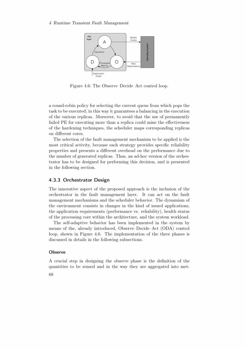
4 Runtime Transient Fault Management
D O
A
Ope
ratin
g Sy
stem
RawObservations
ModifyKnobs
Decisions
ProcessedMetrics
ApplicationGoals
FMlayer
Figure 4.6: The Observe–Decide–Act control loop.
a round-robin policy for selecting the current queue from which pops thetask to be executed; in this way it guarantees a balancing in the executionof the various replicas. Moreover, to avoid that the use of permanentlyfailed PE for executing more than a replica could mine the effectivenessof the hardening techniques, the scheduler maps corresponding replicason different cores.The selection of the fault management mechanism to be applied is the
most critical activity, because each strategy provides specific reliabilityproperties and presents a different overhead on the performance due tothe number of generated replicas. Thus, an ad-hoc version of the orches-trator has to be designed for performing this decision, and is presentedin the following section.
4.3.3 Orchestrator Design
The innovative aspect of the proposed approach is the inclusion of theorchestrator in the fault management layer. It can act on the faultmanagement mechanisms and the scheduler behavior. The dynamism ofthe environment consists in changes in the kind of issued applications,the application requirements (performance vs. reliability), health statusof the processing core within the architecture, and the system workload.The self-adaptive behavior has been implemented in the system by
means of the, already introduced, Observe–Decide–Act (ODA) controlloop, shown in Figure 4.6. The implementation of the three phases isdiscussed in details in the following subsections.
Observe
A crucial step in designing the observe phase is the definition of thequantities to be sensed and in the way they are aggregated into met-
68

4.3 Fault Tolerance through Self-Adaptiveness
rics. They provide a description of the system’s current status as muchcomplete and concise as possible to be useful to make decisions in thesubsequent phase. The following metrics have been identified in orderto observe the two main aspects of interest in the considered multicorescenario: the performance, since such architectures are used as intensivedata processing applications, and the reliability, due to the increasingfailure trend.For estimating the performance, the classical metrics measuring the
execution time are adopted: in particular, the average execution time,and the throughput. In an application modeled through a task-graph(as the example in Figure 2.2) the execution time of a single applicationcycle is measured by evaluating the elapsed time between the beginningof the execution of the first fork node and the end of the execution ofthe last join node:
exec_timeoverall = tend − tstart. (4.1)
Then, the average execution time is computed on a window of the lastn executed cycles.An alternative metric is the throughput. To evaluate this metric, the
orchestrator considers a window of the last n executed cycles of theapplication and computes the ratio between the amount of produceddata and the overall execution time for that window:
throughput =n · dout
tendn − tstart1(4.2)
where dout is the amount of data produced during a single cycle and thecycles are numbered from 1 to n.When referring to reliability, the most relevant issue of the considered
data-intensive computing applications is related to the amount of errorsthey may experience. Thus, the defined reliability-oriented metric mea-sured by the adaptive environment is the detected error rate. Moreover,it is computed on a window of the last n cycles of the application ex-ecution. When considering the application model, we can estimate theerror rate by quantifying the portions of the results produced by faultytasks. Do note that in quantifying the error rate, fault propagation, taskcrashes, and the detection method in use have to be taken into accounttoo.Not all the hardening strategies are able to mitigate the detected er-
rors: in fact, DWC is not able to mitigate errors, and in some scenar-ios other techniques may potentially fail, as discussed in the following.When an error is not mitigated, it will be observed on the final output of
69

4 Runtime Transient Fault Management
Detected #ResourcesError Ratio low high
low TMR < DWCR TMR ∼ DWCR
high TMR ∼ DWCR TMR > DWCR
Table 4.1: Qualitative performance comparison between TMR and DCRtechniques. The comparison refers to the same level of gran-ularity.
the application. Therefore, we also defined the not-mitigated error ratewhich computes this percentage of errors.
Act
During the act phase, the system directly acts on the system knobs,according to the choices taken in the decision phase. In our scenariowe can identify several knobs: the selection of the fault managementmechanism to be applied, the selective application of the mechanism, thegranularity at which it is applied, the possibility to activate or deactivatea processing unit or changing its frequency, and so on. We here focus ona subset of them presented in the following; all the other knobs are leftfor a future investigation.The first considered knob is mechanism selection, that is the choice of
the fault management mechanism to be applied on the running applica-tion. As discussed, each technique has specific properties (fault detec-tion, fault tolerance and fault diagnosis) and performance overhead. Inparticular, the performance for the two mechanisms offering fault toler-ance is listed in Table 4.1. TMR can achieve a greater throughput whenthere is a high number of available processing cores and the system isexperiencing a high error rate: this is due to the fact that resourcesare better exploited when running the three replicas in parallel; DWCRwould not be able to exploit these resources since the third replica wouldbe executed strictly after the first two and a voter will be also executedin addition to the checker. On the other hand, DWCR proved to achievea higher throughput in a scenario with a low error rate and a reducednumber of resources since the third replica is optionally executed. Inthe other two cases the performance of the two techniques depends onthe specific scenario and cannot be classified a-priori. Experimental ev-idences of these considerations will be shown later on.The second knob is the granularity the mechanism is applied at. The
70

4.3 Fault Tolerance through Self-Adaptiveness
granularity represents the possibility to perform a varying placementstrategy of the voter/checker tasks introduced by each fault managementmechanism, thus offering another way to tune the performance/reliabilitytrade-off. We consider only two different granularity levels, even if otherintermediate ones could be added:
• Coarser : checker/voter tasks (according to the considered mecha-nism) are added only after the execution of an independent part ofthe program: after join and fork_join tasks.
• Finer : checker/voter tasks are placed after each task in the task-graph.
The concept of granularity can be, in theory, applied to all the hard-ening techniques. Figure 4.7 shows an example applying the TMR atthe two different levels of granularity on the sample application of Fig-ure 2.2. It is worth noting that in the coarser level only the final resultsare checked/voted, while the possible intermediate results are discarded.Moreover, when the join task has only a synchronization role and hasno data as final output, the voter will test the output data of the childelaboration threads.From a reliability point of view, some combinations of granularity level
and fault management mechanism do not offer any advantage. This isthe case of the DWC that offers the same features for both configurations;however, as discussed later, the performance of the two configurationsdepends on the specific working scenario and therefore it is not possibleto choose the best configuration a-priori. At the opposite, DWCR andTMR offer different reliability properties according to the granularity.When the coarser granularity-level is selected, it is not possible to
guarantee diagnosis features since error propagation effects would be in-troduced and the source of the error would not be identifiable. Moreover,in case of permanent faults, mechanisms offering fault tolerant proper-ties cannot guarantee a 100% coverage, i.e. not all the faults occurringin the system can be actually mitigated by the technique. In fact, themapping constraint of the sibling replicas discussed in Section 4.3.2 al-lows a single permanent processor failure to invalidate tasks belonging todifferent group of replicas before they are voted, as shown in Figure 4.8.In order to guarantee a 100% coverage, the PEs should be partitioned ina number of groups equal to the number of generated replicas, i.e. three.However, since in general the number of processing unit is not multipleof three, this partitioning would imply lower performance. Neverthe-less, even if not providing the full error coverage, these mechanisms stillprovide 100% fault detection coverage.
71

4 Runtime Transient Fault Management
E
F
J
E
V
(a) Coarser Level
E
F
J
E
V
V
V V
(b) Finer Level
Figure 4.7: Application’s task–graph hardened at the two different levelsof granularity: the colored dashed tasks represent the voternodes added to make fault mitigation possible.
E
F
J
E E
F
J
E E
F
J
E
Original 1st Replica 2nd Replica
PE0
PE0
PE0
PE1
PE1
PE1
PE1
PE2 PE0
PE2
PE2
PE2
V
Figure 4.8: If PE0 is permanently faulty, the presented mapping of thetasks on three processing cores, PE0, PE1 and PE2, causesTMR to fail.
72

4.3 Fault Tolerance through Self-Adaptiveness
Granularity #Replicas 100% FD 100% FT Diagnosis
Duplication with Comparison (DWC)
Coarser 2 Yes No NoFiner 2 Yes No No
Duplication with Comparison and re-Execution (DWCR)
Coarser 2/3 Yes No NoFiner 2/3 Yes Yes Yes
Triplication (TMR)
Coarser 3 Yes No NoFiner 3 Yes Yes Yes
Table 4.2: Qualitative evaluation of the described techniques with refer-ence to reliability aspects (FD: Fault Detection – FT: FaultTolerance).
The placement of voter and checker tasks after each node allows DWCRand TMR to achieve a 100% fault tolerance coverage; moreover, thisplacement offers also diagnosis capabilities. Table 4.2 summarizes thereliability aspects presented above.The granularity level has also an impact on performance. Usually,
the selection of the finer granularity level incurs in a higher overhead onthe execution latency with respect to the coarser level, because a largernumber of checker/voter tasks is introduced. However, in some specificsituations the opposite behavior may occur, as we will show in the exper-imental results. More precisely, when the architecture is composed by asmall number of processing units and the application generates a largenumber of parallel threads, the finer granularity level offers the possibil-ity to better schedule on the controller core a larger number of checker/voter tasks comparing the results of the elaboration threads, since theother processing units are overloaded with the execution of the tasks’replicas. Due to this reason, DWC applied at the finer granularity levelhas not been discarded even if it does not offer any advantage from thereliability point of view. Finally, do note that the considerations drawnin Table 4.1 hold at each level of granularity and, more precisely, theserelations are exacerbated as the level of granularity becomes coarser. Inparticular, if the system experiences a high detected error rate, DWCRis highly disadvantageous with respect to TMR since it would require aconsiderable number of tasks to be re-executed.
73

4 Runtime Transient Fault Management
The last knob is the resource activation/deactivation. As discussed inthe description of the fault management techniques, during the execu-tion, the orchestrator may diagnose a suspected damaged PE. In thiscase, it can deactivate the PE in order to further analyze it by means ofspecific diagnosis tasks. A PE can be deactivated by simply removing itfrom the list of the available resources used by the scheduler. Later, ifthe result of the accurate analysis is negative, the PE can be reactivatedand used again for executing the application.As a final remark, do note that knobs can be adjusted only between two
different iterations of the application execution for allowing the contextswitch. This is particularly true for the fault management mechanismssince it is quite complex, even not unfeasible, to adapt internal dataand synchronizations related to replicas and checker/voter tasks from amechanism to another one.
Decide
The decision phase is implemented by the orchestrator through a rule-based decision policy. From a high-level point of view, it evaluates thesystem’s current status on the basis of the sensed metrics acquired in theobserve step, and makes a decision on the actions to be taken through theknobs to reach the desired goal, specified as input when the applicationhas been issued.As discussed in the previous sections, the two conflicting aspects on
which the proposed system focuses are performance and reliability; more-over, each one of the considered hardening mechanisms together withthe granularity level of its application imply a specific impact on eachone of the two aspects: some mechanisms obtain a reduced performanceoverhead but limited reliability properties, while other ones achieve highreliability but incurring in a large performance overhead. Thus, the aimof the system is to decide the most suitable mechanism to be adopted ineach situation to achieve a good trade-off between the two aspects. Inparticular, the designed orchestrator allows one to specify the goal foreach issued application, by specifying which of the two aspects has to beconsidered as constraints; consequently, the system will try to adapt itsbehavior to optimize the remaining dimension. The adaptation is evenmore necessary if we consider that the system conditions can evolve: inparticular, different applications with different goals may be issued, andthe architecture may change due to the deactivation of some faulty units.The goal is specified as a threshold on the value of the metrics rep-
resenting the aspect to be controlled (not-mitigated/detected error ratefor the reliability, or average execution time/throughput for the perfor-
74

4.3 Fault Tolerance through Self-Adaptiveness
Fault Tolerance
DWCR F/C
TMRF/C
TUNING
Fault Diagnosis
DWCR F
TMR F
Fault Detection
DWC F
DWC C
TUNING
Figure 4.9: A FSM representation of the decision process in the casereliability is the constrained dimension.
mance). Do note that the orchestrator will try to fulfill the specifiedconstraint, however, there is no guarantee that it will be satisfied com-pletely ; in fact, the various decisions are made at run-time, and thereforeonly at that time it will be possible to know whether the goal can bereached.The implemented decision policy is a simple rule–based system. The
specified goal is used by the system, first to identify the constrainedvariable and the free one, and then to set a threshold used to take adecision. In particular, the idea is to start the execution by choosing,among the hardening mechanisms, the one having, in theory, the bestexpected result for the unconstrained dimension and to analyze the ef-fects on the constraint variable. The value specified as a constraint onthe application is compared with the current value of the metrics: ifthe constraint is met, the mechanism currently in use does not need tobe changed; otherwise, a more appropriate technique is selected. Thisfirst threshold is strict and a mechanism change occurs every time thethreshold is reached. Other thresholds can be determined at run-time byestimating the effects of the available mechanisms on the current statusof the system.
We discuss here the decision policy design when setting the reliabilityas the constrained dimension. The goal is specified together with theinput task-graph as a not-mitigated error rate R1 not to be reached. Thedecision policy can be modeled with a hierarchical finite state machine(FSM) is shown in Figure 4.9. The initial macro-state, labeled faultdetection, forces the system to apply the DWC mechanism, that is theone that has the smallest impact on performance and allows to perfectlykeep track of the value of the current detected error rate. As discussedDWC will only detect the errors without mitigating them. In particular,
75

4 Runtime Transient Fault Management
the first step is a tuning phase that aims at evaluating the performanceachieved by DWC when applied at finer and coarser granularity levels:each one of the two levels is tested for one cycle. Then, the systemevolves in a second state where DWC is applied at the granularity levelthat obtained better performance.
If the not-mitigated error rate threshold R1 is reached, then a mech-anism enforcing the required fault coverage needs to be applied. Thiswill have the effect of reducing the error rate, while penalizing perfor-mance. Therefore, the system evolves in the fault tolerance macro-state.In this macro-state, the decision policy first performs a tuning phase forprofiling the two hardening mechanisms. In particular, for each mecha-nism both the granularity levels are evaluated, and the less convenientone is discarded; then, the decision policy selects the mechanism offeringhigher performance and consequently evolves in the related sub-state.Do note that the performance of DWCR depends on the number of re-quired re-executions while the TMR one is almost constant. For thisreason, the adaptation stage will switch among the two mechanisms (atthe granularity level identified during the tuning phase) according to theperformance monitored during the execution.
If the detected error rate does not decrease in a given executions’ win-dow, it means that some permanent failures may affect the architecture.Therefore, to perform fault diagnosis, the system evolves to the faultdiagnosis macro-stage, which behaves similarly to the previous one butexploiting only the finer granularity level. Note that the tuning step isnot necessary since the techniques have been already tested in the pre-vious macro-state. During the diagnosis activity, based on the analysisof the fault detection on each PE, if a unit is determined to be faulty,it is switched off, and then the orchestrator evolves to the DWC state.Finally, if the detected error rate decreases, the system evolves from amacro-state to the previous one.
The FSM derived for the case of setting reliability as the constraineddimension can be straightforwardly adapted to the case where perfor-mance is the constrained dimension, or the case where a set of batchapplications is issued. In particular, the same thresholding mechanismwill be used, while the specific actions/techniques applied in each statewill be different. Moreover, the described decision phase is clearly ex-tensible with new mechanisms, automatically taken into account duringthe tuning state.
76

4.4 Experimental Results
4.4 Experimental Results
In this section we present the experimental sessions carried out to demon-strate the effectiveness of the orchestrator. First, the experimental set-upis illustrated and, later, the results of the experiments are discussed intwo different paragraphs.
4.4.1 Experimental Set-up
We adopted and enhanced the simulator previously defined for the ex-perimental sessions presented in [25]. The original tool consists of aSystemC transaction level model [1] of the discussed architecture ableto simulate the execution of applications modeled in terms of fork-joingraphs. Thus, we implemented in the SystemC model all the consideredfault management mechanisms, the support for the granularity levels andthe discussed orchestrator.In the performed experimental sessions, we considered a set of com-
monly used parallel applications taken from the case studies. In particu-lar, we present here the results obtained on a specific application alignedwith the application scenario we refer to, that it the edge detector. Wecharacterized it with a static analysis on the source code for building thetask-graphs annotated with the amount of data processed by each task.Moreover, we used an instruction set simulator running a sequential ver-sion of the application for estimating the execution times of the varioustasks, as in [67]; such execution times contains also bus and memoryaccess latencies. Indeed, as noted in [67], when working at this level ofabstraction, interactions among tasks (e.g., resources conflicts) are not ofinterest since they are later considered in more accurate lower-level sim-ulations. In particular we used the ReSP simulation environment [80] forsimulating an ARM7 unit working at 333MHz connected to a memorythrough a bus, each one with a transmission latency equal to 10ns/word.Finally, we also estimated the execution times of the voters and checkersfor the different amount of data to be compared. The resulting task-graph is shown in Figure 4.10, while a subset of the execution times forthe voters and checkers are presented in Table 4.3.We generated fault lists according to an exponential probability distri-
bution over the experiment duration, since it is well suited for describingtransient faults. They were created by varying the failure rate of the dis-tribution in order to stimulate the system in different ways, thus causingmutating environmental conditions. The generated lists obey the singlefailure model assumption. Note that, the considered fault probabilitieshave been created with a high frequency with respect to fault occurrence
77

4 Runtime Transient Fault Management
567us
1859us
50us
567us
567us
567us
14398us
14398us
14398us
14398us
1859us
0 bytes
2000 bytes each
6000 bytes each
0 bytes
0 bytes
RGB tograyscale
edgedetection
Figure 4.10: Task-graph for the edge detector application.
# Data (byte) Checker Voter
2000 byte 423µs 920µs
6000 byte 1237µs 2550µs
Table 4.3: Execution times for voting and checking various amount ofdata.
78

4.4 Experimental Results
in the real world; the aim is to perform a sort of accelerated experi-ment to better highlight the capability of the orchestrator to adapt tothe environment stimuli. Therefore, we expect the system to behavein the same way in the real world scenario, although on a longer timewindow. It is worth noting that the accelerated experiment requires thesize of the window for the metric computation to be shrunk to make theorchestrator more reactive to the higher external stimuli.
4.4.2 First Experimental Session
The goal of the first experimental session is to show how each singlefault management mechanism behaves differently according to the spe-cific scenario, offering a different performance/reliability trade-off. More-over, the orchestrator is able to select, during the execution, the mostsuitable fault management mechanism at each time, outperforming thesingle statically-selected strategies. We considered four different archi-tectures composed of 6, 8, 10 and 12 processing cores, respectively, andwe generated three fault lists F1, F2 and F3 with a failure rate (i.e.,probability of a single processor failure) equal to 0.0005, 0.001 and 0.003every 200µs.In this experimental session we ran the application hardened with all
the available mechanisms, selected at design-time, and with the pro-posed decision policy. Moreover, we tested all the strategies on each pair<architecture, fault list>. The comparison of the various approacheswas performed by executing the application for a specific number of cy-cles (equal to 200), thus mimicking the elaboration of a fixed amount ofdata. We considered a threshold for the not-mitigated error of the 5%and a window for the metrics computations of 10 cycles.The results of the experimental session are presented in Figure 4.11,
where the overall execution times are reported. Each chart presents theresults obtained for each fault distribution when adopting various mecha-nisms on the considered architecture. The average of not-mitigated errorrates confirmed the expected values: 0% for all fault tolerance strategies(since no permanent fault was injected), less than 5% for the proposedadaptation policy, while DWC is not able to mitigate any error. We didnot report them in the figure.From an accurate analysis of the bar charts we can notice that, as ex-
pected, there is not a mechanism that is always prevailing on the otherones, and each of them achieves better performance in a specific scenario.Moreover, the following empirical rules can be inferred. In general, evenif coarser granularity level introduces a smaller number of voter/checkertasks, the finer one is preferable when the number of available processing
79

4 Runtime Transient Fault Management
DWC COARSERDWC FINERDWCR COARSERDWCR FINERTMR COARSERTMR FINERORCHESTRATOR
6 8 10 12Number of Cores
Exec
utio
n Ti
me
[μs]
4×10⁶
5
6
7
8
9
10×106
(a) Fault list F1.
DWC COARSERDWC FINERDWCR COARSERDWCR FINERTMR COARSERTMR FINERORCHESTRATOR
Number of Cores6 8 10 12
Exec
utio
n Ti
me
[μs]
4×10⁶
5
6
7
8
9
10×106
(b) Fault list F2.
DWC COARSERDWC FINERDWCR COARSERDWCR FINERTMR COARSERTMR FINERORCHESTRATOR
6 8 10 12Number of Cores
Exec
utio
n Ti
me
[μs]
4×10⁶
5
6
7
8
9
10×106
(c) Fault list F3.
Figure 4.11: Overall execution times for the edge detector on the variousarchitectures stimulated by each fault list.
80

4.4 Experimental Results
cores is small, as already motivated in Section 4.3.3. In particular, thiscan be observed from the results reported in Figure 4.11 for the archi-tectures with six cores. A detailed investigation of the scheduling Ganttcharts allowed us to highlight the following situation: when the num-ber of PE is limited, voter tasks analyzing intermediate results used inDWC/F do not overload the control core thus achieving an overall betterperformance than DWC/C, that postpones all results’ checking at theend of the application’s replicas execution. This phenomenon is exploitedby the proposed technique that thus achieves better performance.Moreover for DWC and TMR, the break-even point is represented
by the value obtained by multiplying the maximum number of parallelthreads generated by the application by the number of replicas requiredby the mechanism (for instance, for the edge detector, 4×3 for TMR and4×2 for DWC); on the other hand, it is not possible to identify an exactbreak-even point for DWCR even if the trend is similar. The secondconsideration is that the performance of the two granularity levels forDWCR depends also on the fault frequency: in fact, when the frequencyis high the finer level is more convenient since it allows to re-execute onlya reduced portion of the application. A final consideration is that TMRseems not to be convenient in any scenario; however, as shown in thefollowing experiment, it will outperform the other mechanisms when theerror frequency is even higher, i.e., when a permanent fault affects thearchitecture.When considering the proposed adaptation policy (last bar in each
chart), we can notice that it outperforms all the statically selected ap-proaches (DWC should not be considered since it is not able to mitigatethe errors thus producing corrupted results). As expected, the orches-trator is able to select the best mechanism in each instant of time, thusmaximizing the performance while meeting the specified threshold on thenot-mitigated error ratio. The performance improvement on the best ofstatic approaches in each scenario spans from 1% to 13%. In one sce-nario only the orchestrator exhibits worse performance than the DWCRapplied at finer granularity (i.e. on the architecture with 6 cores stimu-lated by the fault list F3); indeed, the limited number of processing unitsin the considered architecture causes a high latency to execute a singlecycle, and, consequently, the orchestrator evolves too slowly to select theappropriate mechanism to mitigate the high frequency of faults.Even if the scenarios presented so far showed the necessity for a dy-
namic mechanism selection, they are not the situations in which theproposed orchestrator shows its effectiveness. In fact, the consideredfault lists have been generated by means of a constant failure rate andno permanent fault has been injected. Therefore, in a second experi-
81

4 Runtime Transient Fault Management
mental session, we aimed at showing the adaptation capability of theorchestrator by considering a fault list generated with a variable failurerate and a permanent fault corrupting a single processing core.
4.4.3 Second Experimental Session
In the second experimental session, we executed the edge detector in ascenario with evolving environmental conditions in terms of fault dis-tribution. For about the first 4, 000s the system experiences a failurerate equal to 0.001 every 200µs; then, from time 4000s to 10, 000s thisprobability is increased to 0.003 every 200µs: in this way the behaviorof the system when a varying failure rate occurs is tested. To make thescenario more complete and complex, at time 10s a permanent failureis injected in one of the architecture cores. The edge detector is run for600 cycles on an architecture made up of 12 cores.The first plot (Figure 4.12(a)), aims at showing which is the system’s
behavior perceived from the outside. The top part of the graph shows thenumber of detected and not-mitigated errors experienced at each cycleby the system. This allows to figure out the role played by the faultmitigation techniques in reducing the number of visible faults. Finally,the gray vertical areas describing the used hardening approach in eachtime interval.The second plot (Figure 4.12(b)) shows the internal status of the or-
chestrator, and in particular presents the values of the metrics on whichthe orchestrator makes decisions on the mechanism to select at eachexecution cycle. On the top graph, the average window values for thedetected and not-mitigated error rates are plot (for this experiment awindow value of 20 cycles was chosen), while the dashed horizontal lineat value 0.05 represents the reliability constraint specified by the user. Inthe bottom plot the average window value for the performance is shown.Therefore, the orchestrator selects a specific mechanism according to thecurrent values of the metrics; the selected mechanism is reported bymeans of gray areas of different intensity.By looking at all the graphs, it is possible to see how the proposed
approach actually allows to adapt the behavior of the considered systemto cope with the mutating fault distribution. Indeed, at the beginningof the execution, when the failure rate is relatively low, the orchestratordecides not to mitigate any fault, but only to detect them. When thenumber of detected errors becomes too high, the orchestrator performsa tuning phase, analyzing the performance of the techniques providingfault tolerance. Thus, in this first phase, DWRC at the finer level isselected to be executed alternatively to DWC at the coarser level. When
82

4.4 Experimental Results
TMR C TMR C
DWC C DWC C DWC CDWC C TMR F
TUNING DWCR F
Number of Not Mitigated ErrorsNumber of Detected Errors
C: coarser granularityF: finer granularityDWC C
Permanent Fault InjectedExec
utio
n Ti
me
[μs]
30000
40000
Num
ber o
f Erro
rs [b
it]
0
10000
20000
Execution Cycle0 50 100 150 200 250 300 350 400 450 500 550 600
(a) Execution latency, and number of detected/not-mitigated errors at each cycle.
TMR C TMR C
DWC C DWC C DWC CDWC C TMR F
TUNING DWCR F
DWC C
Not Mitigated Error RateDetected Error Rate
C: coarser granularityF: finer granularity
Permanent Fault InjectedExec
utio
n Ti
me
[μs]
25000
30000
Erro
r Rat
io
0
0.2
0.4
0.6
0.8
Execution Cycle0 50 100 150 200 250 300 350 400 450 500 550 600
(b) Average execution latency and detected/not-mitigated error rates over the specifiedwindow.
Figure 4.12: Metrics computed over the overall experiment execution.
83

4 Runtime Transient Fault Management
the failure probability increases, DWRC performance is no more satis-fying and TMR at the coarser level becomes the chosen fault tolerantmechanism, to be executed in alternative to DWC. Finally, from aboutthe 370th execution cycle, the orchestrator identifies an even higher er-ror ratio suspecting the presence of a permanent fault and definitivelyswitches to TMR applied at the finer level to perform the fault diagnosis;if the response is positive, the orchestrator will switch-off the damagedPE and will apply again DWC.As a final note, Figure 4.13 compares the throughput achieved by the
presented approach with all the other statically selected mechanisms alsowith respect to the plain execution; on each bar the relative percentagevalue with respect to the plain execution is reported. As discussed above,DWC applied at both levels obtains best performance but it violates thereliability requirement on the error ratio. Then, when considering theother strategies, the orchestrator obtains an improvement of only the 5%with respect to the TMR at coarser level; however, this mechanism isnot able, in the second part of the experiment, to perform fault diag-nosis. Thus, a fair comparison can be performed only with TMR andDWCR applied at finer level since they offer all the discussed reliabilityproperties; in such a scenario, the orchestrator obtains an improvementof 18% and 23% respectively, thus demonstrating its effectiveness. Asa final note, the throughput of the plain execution is not considerablyhigher than hardened ones as it may expect. This is due to the fact thatthe number of threads generated by each fork is decided at design-time(equal to 4) and therefore it is not possible to fully exploit the archi-tecture capabilities; a possible future development of the approach mayconsider the dynamic decision of the number of threads as also supportedin OpenMP [95].
4.5 Final Remarks
In this chapter we introduced the design of an self-adaptive system andrelated orchestrator for fault management in multicore architectures,able to monitor and adapt itself in order to pursue the desired perfor-mance/reliability trade-off. The orchestrator is implemented in a faultmanagement layer working on top of the operating system, in chargeof providing reliability properties when desired. The proposed solutiondynamically selects and applies fault detection/tolerance mechanisms tomitigate the effects of faults while optimizing performance. Experimen-tal results performed in the image processing scenario show that theprovided self-adaptability feature allows to achieve better performance
84

4.5 Final Remarks
NOT HARDENEDDWC FINERDWC COARSERDWCR FINER
DWCR COARSERTMR FINERTMR COARSERORCHESTRATORFault Detection
Fault Detection & Mitigation
72.97%100% 79.10% 54.80% 48.55% 57.33% 64.31% 67.46%
Reliable Technique
Thro
ughp
ut [K
B/s]
0
200
400
600
800
1000
1200
1400
Figure 4.13: Throughput for the edge detector on the architecture with12 processing cores, stimulated with a fault list presentinga variable failure rate and a permanent fault.
while fulfilling the reliability requirements with respect to traditional,static solutions.
In the next chapter a self-adaptive system for extending architecturelifetime through age mitigation (while minimizing energy consumption)will be presented. It is based on the same autonomic control loopparadigm, but exploits different monitors, decision policies and knobsto achieve such goal.
85


5 Runtime Aging Management
This chapter describes a novel self-adaptive system for mitigating agingin multi/manycore architectures. In the first part of the chapter thelifetime evaluation process will be presented and the design of a frame-work for lifetime estimation discussed. The remainder is devoted to thepresentation of runtime resource management policies for extending ar-chitecture lifetime, both at the node and at the multi-node level, whileminimizing energy consumption and meeting performance constraints.
5.1 Background
The first step in extending the system lifetime is to be able to measureit. This activity is particularly challenging when considering a com-plex multicore architecture with possibly multiple and subsequent PEfailures, and when supporting runtime resource management strategies,whose effects on cores’ aging and wear-out is a-priori unknown. Shouldsensors be available, it would be a matter of accessing their information.However, in a generic architecture such sensors are not available and it isnecessary to estimate the aging of a core or a system by referring to theperformed activity and the working conditions. When these aspects varyduring the life of the system, the computation may be particularly com-plex. We here first discuss how we estimate the aging, then we introducethe tool to support such computation.
Reliability of a single system at time t, R(t), is usually referred toas the probability that the system has been operational until t. Assuggested by the JEDEC Solid State Technology Association [57], thelifetime reliability of a single digital component, such as a PE, can bemodeled according to the Weibull distribution
R(t, T ) = e−(
tα(T )
)β, (5.1)
being t the current instant of time (generally measured in hours), Tthe (steady-state) PE temperature (Kelvin degrees), β the Weibull slopeparameter (considered to be independent of the temperature), and α(T )the scale parameter [52]. The lifetime of the PE is estimated in terms of
87

5 Runtime Aging Management
its Mean Time To Failure (MTTF), defined as the area underlying thereliability function R(t, T ):
MTTF =
∫ ∞0
R(t, T ) · dt. (5.2)
The α(T ) parameter formulation depends on the wear-out effects to bemodeled, such as [57]: electromigration (EM), thermal cycling (TC),time-dependent gate oxide breakdown (TDDB), or negative-bias tem-perature instability (NBTI). As a proof of concept, EM related wear-outfailures will be considered for the framework validation in the experi-mental results. In the EM model, Black’s equation is used to computeα(T ):
α(T )EM =A0(J − Jcrit)
−neEakT
Γ(
1 + 1β
) (5.3)
where A0 is a PE-dependent constant, J is the current density, Jcrit isthe critical current density for the EM effect to be triggered, Ea is theactivation energy for EM, k is the Boltzmann’s constant, n is a material-dependent constant, β the slope parameter of the Weibull distributionand Γ() is to the gamma function. However, it is possible to integrateother effects either as standalone contributes or by using the sum-of-failure-rates (SOFR) approach for any combination of the above failureeffects [90]. In fact, in the second part of the chapter (when DVFScomes into play), thermal cycling will also be considered. Coffin-Mansonequation [57] can be used to model TC effects and α(T ) can be writtenas:
α(T )TC = C0(∆T −∆T0)−qf. (5.4)
where ∆T represents the temperature cycling range and ∆T0 the elasticportion of the thermal cycle (typically, ∆T0 << ∆T , thus ∆T0 can bedropped from Equation 5.4); C0 is a material dependent constant, q isthe Coffin-Manson exponent, and f is the frequency of thermal cycles.In conclusion, by exploiting the SOFR model, α(T ) due to both TC andEM is given by the sum of α(T )EM and α(T )TC .To formulate R(t) for the general scenario of a multicore system shar-
ing a variable workload, the above formulas need to be revised to con-sider two specific aspects: i) temperature changes due to a variationin the workload, and ii) system composition in terms of its resourcesand its capability to survive beyond the first failure. These two aspectsare here now briefly presented in relation to the scenario of the pro-posed approach; for a more precise formulation, it is possible to refer
88

5.1 Background
timeline0 t1 t2 ti-1 ti
T1 T2 TiTemperature:
Figure 5.1: Model of a PE’s temperature profile over time.
RR
EMAP
t1 t
R(t)
workload change
R(t,T1)R(t - t1 + t1,T2)^
Rel
iabi
lity
0
1
Time [h]0 1×10⁵
RR
EMAP
t1t1̂
R(t,T2) has tobe rightshiftedto connect thetwo curves in t1
R(t,T1)R(t,T2)
Rel
iabi
lity
0
1
Time [h]0 1×10⁵
Figure 5.2: Reliability curve considering temperature changes.
to [69, 51]. When the temperature changes as shown in Figure 5.1 (tokeep the computation manageable, steady-state temperatures are con-sidered), the exact computation of the R(t) function is computed usingEquation 5.1 and its inverse function, R−1(r, T ), defined as:
R−1(r, T ) = α(T ) · (−log(r))1/β (5.5)
being r a reliability value. The R−1(r, T ) function returns the elapsedtime t, starting from time 0, when the system reaches the reliabilityvalue of r, under the influence of a fixed temperature T . In particular,the R(t, T1) function can be directly applied only to a new PE (i.e.,when t < t1, being t1 the time when a load redistribution takes placecausing a change in the steady-state temperature). On the other hand,when t ∈ (t1, t2], the PE reliability is equal to R(t − t1 + t̂1, T2), wheret̂1 = R−1(r1, T1) and r1 is the reliability value in t1 [69]. Similarly, thesystem’s reliability for values of t in the next steps can be computedwith a recursive approach by using the above-mentioned formulas. Froma graphical point of view (shown in Figure 5.2), R(t, T ) is a curve startingfrom t = 0 (and R(0, T ) = 1) with a varying shape that depends on thetemperature T . Therefore, at each temperature change it is necessaryto right-shift the new reliability curve in order for it to intersect the oldreliability value. Finally, the R(t) formula considering a variable PE’s
89

5 Runtime Aging Management
temperature can also be rewritten in the following way [101]:
R(t) = e−(∑i
j=1
τjαj(T )
)β. (5.6)
where τj represents the duration of each period of time with constanttemperature Tj up to time t (i.e., t =
∑ij=1 τi).
All the equations discussed so far refer to the case of a system with asingle PE. Let us now move to a system consisting of n PEs subject to asequence of k failures, causing a redistribution of the workload after eachfailure occurrence. Such scenario is usually referred to as a load-sharingk-out-of-n:F system, made up of non-independent and non-identicallydistributed (non-i.i.d.) variables with arbitrary distribution. k (≤ n) isthe minimum number of PEs that have to fail before the entire systembecomes out-of-service. The reliability of such system is computed byusing the total probability formula:
R(t) = Pno_f (t) + P1_f (t) + · · ·+ Pk−1_f (t). (5.7)
Pno_f (t) is the probability that no failure occurred and is computed asthe product of the reliability of all PEs:
Pno_f (t) =
n∏i=1
Ri(t). (5.8)
We call the MTTF to the first failure the integral between 0 and +∞of such formula; as discussed above, several works [50, 58, 29, 54] ap-proximate the system MTTF to such value. P1_f (t) is the sum of theprobabilities of occurrence of n different cases where a single PE failsand its load is redistributed onto the other working units:
P1_f (t) =
n∑i=1
∫ ∞0
fi(t1) ·n∏
j=1,j 6=iRj(t|ti1)dt1 (5.9)
where fi(t) is the probability density function of Ri(t), i.e., the probabil-ity that the failure occurred on PE i at a specific time t1, and Rj(t|ti1)is the conditioned reliability function of PE j knowing that PE i failedat time t1. It is worth noting that conditioned reliability functions canbe computed by using the formulas for load remapping, as shown in [69].Similarly, P2_f (t) is computed as:
P2_f (t) =
n∑i=1
n∑j=1,j 6=i
∫ ∞0
∫ t2
0fi(t1) · fj(t2|ti1)· (5.10)
·n∏
m=1,m6=i 6=jRm(t|ti1, t
j2) · dt1 · dt2 (5.11)
90

5.2 Aging Evaluation
by using probability density functions and the reliability function con-ditioned by the previous sequence of failures, the first one occurred att1, the second one at t2>t1. Finally, the general scenario considering thesequence of k − 1 failures is a (k − 1)-dimensional integral that can bewritten recursively on the basis of Equations from (5.7) to (5.10).
5.2 Aging Evaluation
The existing solutions for aging evaluation and lifetime estimation ([50,58, 101, 43]) are either too simplistic (e.g., they consider the system to failafter the first PE fails) or are limited in the features (e.g., homogeneousworkload distribution and static design-time mapping), not allowing thedesigner to fully estimate the system’s lifetime in a dynamic workingscenario. In the following we report a review of the literature highligthingthe limitations our proposal aimed at overcoming.
5.2.1 State of the Art
Devices aging and wear-out mechanisms (such as EM, TC, TDDB, andNTBI) have been accurately studied and modeled [57]. These modelsusually consider a homogeneous device and assume a single steady-stateoperation mode at fixed (worst-case) temperature. These aspects con-stitute a significant limitation when taking into account modern systemscomposed of many processors, working in highly dynamic contexts, interms of both the executed workload and its distribution on the PEs,elements that highly affect system’s aging rate.One of the first system-level models for lifetime reliability evaluation
is presented in [90]; it uses a SOFR approach to take into account severalaging mechanisms. The proposed approach, as well as subsequent ones,considers a single core architecture [33] or adopts exponential failuredistributions [58] that are though unable to capture accumulated agingeffects. As a result, they are not suitable for multicore architecturessupporting load-sharing.When using Weibull or lognormal distributions to consider the aging
history, as in [50] and [101], an important issue related to the computa-tional complexity of the lifetime reliability evaluation arises. In fact, ineach instant of time, the reliability of each component is a function ofthe current working conditions and the aging effects accumulated in theprevious periods of activity. Actually, the simulation of the overall lifeof the system capturing the workload evolutions is a prohibitive time-consuming activity. Therefore, many approaches [58, 50, 101] simulateand trace only a subset of representative workloads for a reduced period
91
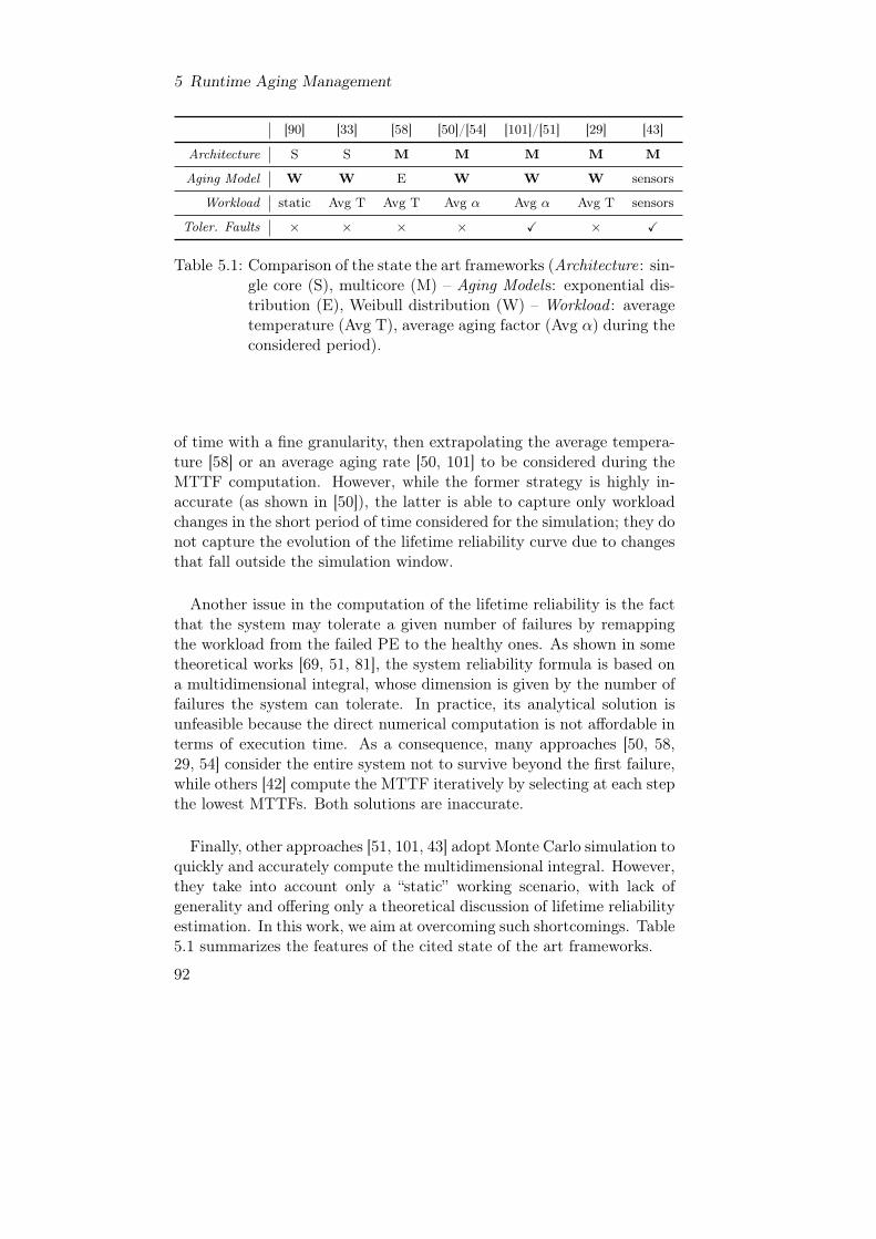
5 Runtime Aging Management
[90] [33] [58] [50]/[54] [101]/[51] [29] [43]
Architecture S S M M M M M
Aging Model W W E W W W sensors
Workload static Avg T Avg T Avg α Avg α Avg T sensors
Toler. Faults × × × × X × X
Table 5.1: Comparison of the state the art frameworks (Architecture: sin-gle core (S), multicore (M) – Aging Models: exponential dis-tribution (E), Weibull distribution (W) – Workload : averagetemperature (Avg T), average aging factor (Avg α) during theconsidered period).
of time with a fine granularity, then extrapolating the average tempera-ture [58] or an average aging rate [50, 101] to be considered during theMTTF computation. However, while the former strategy is highly in-accurate (as shown in [50]), the latter is able to capture only workloadchanges in the short period of time considered for the simulation; they donot capture the evolution of the lifetime reliability curve due to changesthat fall outside the simulation window.
Another issue in the computation of the lifetime reliability is the factthat the system may tolerate a given number of failures by remappingthe workload from the failed PE to the healthy ones. As shown in sometheoretical works [69, 51, 81], the system reliability formula is based ona multidimensional integral, whose dimension is given by the number offailures the system can tolerate. In practice, its analytical solution isunfeasible because the direct numerical computation is not affordable interms of execution time. As a consequence, many approaches [50, 58,29, 54] consider the entire system not to survive beyond the first failure,while others [42] compute the MTTF iteratively by selecting at each stepthe lowest MTTFs. Both solutions are inaccurate.
Finally, other approaches [51, 101, 43] adopt Monte Carlo simulation toquickly and accurately compute the multidimensional integral. However,they take into account only a “static” working scenario, with lack ofgenerality and offering only a theoretical discussion of lifetime reliabilityestimation. In this work, we aim at overcoming such shortcomings. Table5.1 summarizes the features of the cited state of the art frameworks.
92
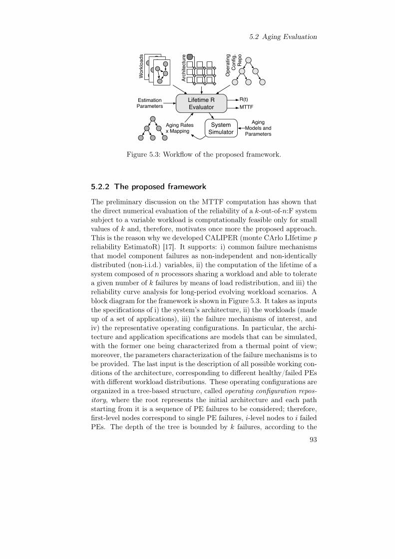
5.2 Aging Evaluation
Lifetime R Evaluator
Wor
kload
s
Arch
itect
ure
Ope
ratin
gCo
nfig.
Repo
EstimationParameters
Aging Ratesx Mapping
SystemSimulator
AgingModels andParameters
R(t)MTTF
Figure 5.3: Workflow of the proposed framework.
5.2.2 The proposed framework
The preliminary discussion on the MTTF computation has shown thatthe direct numerical evaluation of the reliability of a k-out-of-n:F systemsubject to a variable workload is computationally feasible only for smallvalues of k and, therefore, motivates once more the proposed approach.This is the reason why we developed CALIPER (monte CArlo LIfetime preliability EstimatoR) [17]. It supports: i) common failure mechanismsthat model component failures as non-independent and non-identicallydistributed (non-i.i.d.) variables, ii) the computation of the lifetime of asystem composed of n processors sharing a workload and able to toleratea given number of k failures by means of load redistribution, and iii) thereliability curve analysis for long-period evolving workload scenarios. Ablock diagram for the framework is shown in Figure 5.3. It takes as inputsthe specifications of i) the system’s architecture, ii) the workloads (madeup of a set of applications), iii) the failure mechanisms of interest, andiv) the representative operating configurations. In particular, the archi-tecture and application specifications are models that can be simulated,with the former one being characterized from a thermal point of view;moreover, the parameters characterization of the failure mechanisms is tobe provided. The last input is the description of all possible working con-ditions of the architecture, corresponding to different healthy/failed PEswith different workload distributions. These operating configurations areorganized in a tree-based structure, called operating configuration repos-itory, where the root represents the initial architecture and each pathstarting from it is a sequence of PE failures to be considered; therefore,first-level nodes correspond to single PE failures, i-level nodes to i failedPEs. The depth of the tree is bounded by k failures, according to the
93

5 Runtime Aging Management
designer’s specifications. Each node (called operating configuration) inthe tree is annotated with a set of mappings, each one describing howthe workload is distributed on the healthy PEs. There will be a singlemapping in the scenario where changes in the workload distribution areonly triggered by a PE’s failure. Otherwise, when a dynamic workloadscenario is envisioned, the time plan of the various workloads will beprovided, by listing the set of considered mappings, each one with itsown duration.CALIPER is internally organized into two modules: the lifetime reli-
ability evaluator and a supporting system simulator. The first module,the core of the proposed work, performs the lifetime reliability evalua-tion for the overall system by means of Monte Carlo simulations; moreprecisely, it estimates the system’s reliability curve R(t) and its expectedlifetime, in terms of MTTF. To perform such computation, the evalua-tor module requires the aging characterization for the architecture’s PEs.This characterization must be computed under the influence of the ex-ecuted workload in all operating configurations (and related mappings)considered in each specific Monte Carlo simulation. Therefore, the sys-tem simulator is invoked once for each considered mapping to estimatethe thermal profile of the PEs and to derive their aging rates α(T ). Theinternals of the two modules are described in details in the following.
Aging rates estimation
The simulation engine is a service module used to characterize the life-time reliability of the system at processor level; it receives as input theoperating configuration and the mapping, and produces as output thereliability characterization of each PE within the architecture for thatscenario, in terms of the average aging rate. To this end, the main ac-tivity of this module is to estimate the thermal profile of each PE withrespect to the given workload distribution.Within the same operating configuration mapping, PE’s temperature
varies significantly from application to application and, at a finer granu-larity, with different applications’ tasks; moreover, it is also affected bythermal interferences with neighbor units on the architecture floorplan.As an example, Figure 5.4 reports the thermal profile associated withthe execution of a given application, modeled by a periodic task graph,with respect to a given mapping (containing also the scheduling infor-mation): the temperature of a PE depends also on the activity of theneighbor units, running their part of the application. Thus, architectureand application models have to capture all these aspects; more detailswill be provided in Section 5.2.3 for the specific solution we adopted in
94

5.2 Aging Evaluation
2
1
2 3
4
C2
C1 1 3 4
t0 t1 t2 t3 t4
T10 T11 T12 T13
T20 T21 T22 T23timeline
Figure 5.4: Example of application execution and thermal profile.
the proposed framework prototype.Since for each mapping in the operating configuration repository the
workload is almost stationary, as shown in [101], it is not necessary tosimulate the system for its complete life and to compute the reliabilitycurve by means of Equation 5.6; such activity would be actually compu-tationally non affordable. Indeed, it is possible to compute the averageaging rate by tracing the system execution for a representative time pe-riod and by using the following formula:
α =
∑pi=0 τi∑p
i=0τi
αi(T )
(5.12)
where τi represents the duration of the p atomic steps (with constanttemperature on each PE) within the simulated period. Then, the reli-ability evaluator uses such values as input parameters in Equations 5.1and 5.5 to derive the lifetime reliability of the overall system. As a finalnote, even if simulated times may span from few microseconds to severalhours, the result is the average aging per time unit, since Equation 5.12is a ratio between the accumulated aging rates and the time window;considering the units of measure of the various parameters, the α valueis generally referred per hour.
Reliability computation
The second module of the framework is devoted to the evaluation ofthe lifetime reliability curve R(t) of the entire system and the relatedMTTF. Since numerical evaluation of the model presented in Section 5.1is computationally unsustainable for more than 4 subsequent failures (asshown in Section 5.2.3), this activity is performed by means of MonteCarlo simulations to greatly reduce the computational time while ob-taining accurate results. In the following paragraphs, the basic approachis discussed in details, and two improvements are then presented: i) the
95
5 Runtime Aging Management
automatic tuning of the number of simulations needed to obtain a cer-tain confidence in the obtained results and ii) the handling of variableworkloads.The basic scenario we consider (non-i.i.d. load-sharing) is character-
ized by a change in the workload distribution on the healthy PEs onlywhen a PE fails. Multiple subsequent failures are considered: the wholesystem fails when the number of healthy PEs is below a threshold spec-ified by the designer. The pseudo-code for the lifetime computation isshown in Algorithm 1 and here briefly explained. Before getting into thedetails, for readability’s sake, it is worth redefining the two functions R()and R−1(), describing the reliability of a single PE, to take as input theα parameter, computed by means of the system simulator, in place ofthe temperature T . The inputs of the algorithm are: i) the number n ofPEs in the architecture, ii) the number of failures k that causes the entiresystem to become out-of-service, and iii) the number of simulations tobe performed #iter.A single Monte Carlo test consists of a simulation of a randomly-
chosen sequence of PE failures’ events; the goal is to compute the timeto failure (TTF) of the overall system during that specific simulation.To compute the lifetime reliability, the same procedure must be iterated#iter times. After an initialization phase (Lines 2–5), the random walkstep takes place and is repeated until the number of healthy PEs reachesn-k (Lines 7–27). Starting from a completely healthy architecture, foreach iteration a specific subset of healthy PEs with a given workload dis-tribution is selected and a failing event happens; the PE failing at time tis randomly chosen among the healthy ones. This failure triggers the up-date of the system reliability based on the ones of the remaining healthyPEs. To compute the α values for each step, the getAlpha() function isused; it invokes the simulation engine by specifying the current operatingconfiguration currConfig. For all the healthy PEs i, a new reliabilityvalue randR is randomly chosen within [0, currR[i]] (Line 11): it repre-sents the reliability at which that PE will fail. The corresponding timeinstant t (all times are measured in hours) for such failure is computed(Line 12). Moreover, the time period between the current failure andthe subsequent one needs to be computed, by evaluating the equivalenttime eqT and subtracting it to t (Lines 13–14, please refer to Section 5.1for the theoretical details). After having computed the failure times forall healthy PEs, the smallest one is selected to identify the next event,i.e., the next PE to fail; the simulation is thus advanced until such t,the PE is removed from the list of healthy ones (Lines 21–22), and thereliability values of all remaining PEs are updated (Line 24), to beginwith a new iteration. At the end of each simulation, the value called
96

5.2 Aging Evaluation
MTTFm is updated by computing the sample mean of the system’s TTFvalues experienced in the last m iterations (Line 29).When all the simulations have been performed, collected data are sum-
marized by generating the system reliability curve (Lines 32–39); for eachtime t corresponding to a failure, the value of R is computed as the ratiobetween the number of simulations with time greater than the currenttime and the total number of performed simulations. Finally, the algo-rithm displays the reliability curve and returns the MTTFm, representingthe MTTF of the system updated to the last iteration.
Since Monte Carlo simulations are a stochastic approach, it is neces-sary to assess a certain level of accuracy in the obtained results. Thus,the basic algorithm has been enhanced to automatically tune the numberof tests #iter to be performed to obtain a given confidence level. Theprogram iterates the simulations until either a specified percentage c%of the width of the confidence interval for the MTTFm value is less thana given threshold th, or the maximum number of iterations #maxiter isreached (to avoid starvation). The first condition is expressed as:
2 ·Ψ−1(
1 + c%
2
)· cv[TTFm]√
m≤ th (5.13)
where m is the number of performed tests, cv[TTFm] is the coefficient ofvariation of the m TTF samples considered (i.e., the same ones used to
estimate MTTFm), computed as√V ar[TTFm]
MTTFm, and Ψ−1(x) is the inverse
of the cumulative normal distribution. c%, th and #maxiter are receivedas input in place of #iter.
Frequent workload remappings can be approximated by using averageaging rates as demonstrated in literature [50]; however, when consideringlong-term workload changes, such method may not be accurate enough.To this purpose, the framework supports the specification of a sequenceof mappings for each operating configuration, each one provided with itsduration. Algorithm 1 has been slightly revised to support such aspect;more precisely, the computation of the new reliability value (Line 12) isreplaced with the code snippet listed in Algorithm 2: it performs a step-by-step update of the reliability value and related elapsed time by usingR() and R−1() functions (as already described in Section 5.1) based onthe specified workload time plan. Do note that getCurrMapping() andgetTimeToNextChange() functions return the mapping and the relatedperiod for the current operating scenario. Correspondingly, the reliabilitycomputation of the remaining healthy PEs upon a PE failure (Line 24in Algorithm 1) needs to be adapted as well, with a similar strategy.
97

5 Runtime Aging Management
Algorithm 1 Monte Carlo-based reliability computation1: for m = 1 to #iter do2: currConfig = getInitConfig()3: healthy = {0, 1, ..., n− 1}4: currR = {1, 1, ..., 1}5: totalT ime = 06: TTFAccumulator = 07: while size(healthy) > n− k do8: failingPE = −19: alpha = getAlpha(currConfig)10: for all i in healthy do11: randR = random() · currR[i]12: t = R−1(randR, alpha[i])13: eqT = R−1(currR[i], alpha[i])14: t = t− eqT15: if failingPE == −1 or failT ime > t then16: failingPE = i17: failT ime = t18: prevEqT ime = eqT19: end if20: end for21: totalT ime = totalT ime+ failT ime22: healthy.remove(failingPE)23: for all i in healthy do24: currR[i] = R(failT ime+ prevEqT ime, alpha[i])25: end for26: currConfig = updateConfig(failingPE)27: end while28: TTFAccumulator = TTFAccumulator + totalT ime29: MTTFm = TTFAccumulator/m30: stats[totalT ime] + +31: end for32: currHealthyIter = #iter33: precT = 034: for all t in stats.keys() do35: currHealthyIter = currHealthyIter − stats[entry]36: currRvalue = currHealthyIter/#iter37: precT = t38: print t, currRvalue39: end for40: return MTTFm
98

5.2 Aging Evaluation
Algorithm 2 Computation of the next PE to fail for dynamic workloadchangesInput: currConfig, randR, currR[i], alpha[i], totalT imeOutput: t1: currMapping = getCurrMapping(currConfig, t)2: period = getT imeToNextChange(currConfig, t)3: t = totalT ime4: alpha = getAlpha(currConfig, currMapping)5: eqT = R−1(currR[i], alpha[i])6: testR = R(eqT + period, alpha[i])7: while testR > randR do8: t = t+ period9: currR[i] = testR
10: currMapping = getCurrMapping(currConfig, t)11: period = getT imeToNextChange(currConfig, t)12: alpha = getAlpha(currConfig, currMapping)13: eqT = R−1(currR[i], alpha[i])14: testR = R(eqT + period, alpha[i])15: end while16: if currR[i] > randR then17: eqT = R−1(currR[i], alpha[i])18: lastT = R−1(randR, alpha[i])19: t = t+ lastT − eqT20: end if21: return t
99

5 Runtime Aging Management
5.2.3 Experimental evaluation
A SystemC discrete event simulator (with a structure similar to [54,36, 21, 50]) has been developed, while HotSpot [87] has been used tocharacterize the architecture’s thermal profile. Do note that CALIPERcan be integrated in a state-of-the-art framework, such as the one in [32].
The system considered in the experimental sessions is a mesh-basedSystem-on-Chip architecture with N ×M PEs, spanning from 2 × 1 to3 × 4. The system executes a workload that is uniformly distributedamong the healthy PEs, such that all PEs have a 50% occupation in theinitial healthy architecture. The workload is then redistributed after theoccurrence of each failure and/or a given period. In the experiments, weconsider the system to be out-of-service when, after a remapping, theworkload per PE is higher than 100%. Finally, the EM-related parame-ters have been borrowed from [54].
Approach Validation
The approach has been validated against the exact formulation presentedin Section 5.1 based on multidimensional integrals. The exact model hasbeen solved by means of numerical methods (step discretization and rect-angles). The discretization step has been set to 500 hours, causing anoverall negligible error, since the R() curve is almost equal to zero at400, 000 hours, in a 1-out-of-2:F scenario. Due to the high computa-tional complexity of exact approaches, validation against them has beenfeasible for architectures with at most 2 × 3 PEs, tolerating up to 3failures. In all the performed tests, the observed difference between theMTTF computed by means of exact approaches and the one computedby means of CALIPER is lower than 1%; do consider that such errormay also be related to the discretization step. All the scalability experi-ments discussed in this section have been run with a constant workloadthroughout the whole system lifetime.The main scalability problem of the exact method is related to the
(k − 1)-dimensional integral to be solved for a system failing after kfailures (Equation 5.7). Such an integral has an asymptotic complexityO(tk), being t the overall simulation duration. In fact, when consideringa 2 × 3 architecture, the exact method took less than 3 seconds forcomputing the MTTF for k = 1 or k = 2 failures; the computationtime increased to 1 minute and 10 seconds for 3 failures, while requiringmore than 2 hours for 4 failures. On the other hand, the executioncomplexity of CALIPER scales almost linearly w.r.t. the number of
100

5.2 Aging Evaluation
performed iterations and the number of simulated failures, as shown inFigure 5.5, which considers a 3× 4 architecture. We measured the sameerror (< 1%) in the experiments for which we were able to perform thevalidation. Do consider that aging rates have been precomputed andtabulated in an input file to perform an analysis of the performance ofthe Monte Carlo simulations approach only.It is also interesting to analyze how the number of iterations for a fixed
width of the confidence interval (c% = 95%) and threshold parameter(th = 0.1) changes with reference to the considered architecture and thenumber of failures k. Figure 5.6 shows that the number of iterations isalmost constant if k is fixed, regardless of the considered architecture’sdimension and topology, and more important, it decreases as k grows.This could seem to be a surprising result, but the explanation is actuallyintuitive: as it can be seen in Equation 5.13 the width of the confidenceinterval (i.e., the left side of the inequality) is proportional to the coef-ficient of variation cv[TTFm]. By increasing the number of failures, thecoefficient of variation decreases and the number of required iterationsfor the algorithm to converge decreases as well. Figure 5.7 empiricallyproves this trend. A theoretical proof of this behavior can be providedfor the exponential case, since the corresponding distribution becomeshypoexponential; the same idea holds for the Weibull case.
Constant workload scenarios: comparison
CALIPER has been compared against some state-of-the-art approachesassuming a constant workload scenario:
• the Mean Time To First Failure (FF ), adopted in [50, 58, 29, 54],where the whole architecture is considered to be out-of-servicewhen the first PE fails. In this case the reliability is computedby exploiting Equation 5.7;
• the sum of MTTF (Sum), proposed in [42]: in this case, at eachstep, the PE selected to fail is the one with the lowest MTTF,the reliability for the healthy PEs is updated and a new step iscomputed, until the architecture cannot reach the required perfor-mance;
• the worst case temperature (wc) [57]: at each step, the worst casetemperature in the architecture is considered for computing thesystem aging.
Figure 5.8 reports the obtained results for such a comparison. While allthe considered approaches have comparable execution times (same trend
101

5 Runtime Aging Management
100,000250,000500,0001,000,000
Iterations
Tim
e [s
]
0
20
40
60
Number of Failures k0 1 2 3 4 5 6 7
Figure 5.5: Simulations execution times w.r.t. number of failures k.
1234
567
FailuresItera
tions
0
1
2
3
4×10⁶
Architecture2x1 3x1 2x2 2x3 2x4 3x3 2x5 3x4
Figure 5.6: Iterations number w.r.t. different architectures topologies.
2x13x12x22x3
2x43x32x53x4
Architecture
Coe
ffici
ent o
f Var
iatio
n
0.2
0.3
0.4
0.5
Number of Failures k1 2 3 4 5 6 7
Figure 5.7: Coefficient of variation w.r.t. number of failures k.
102

5.2 Aging Evaluation
7h failure6th failure5th failure4th failure
3rd failure2nd failure1st failure
CAL
IPER
Firs
t Fai
lure
MTT
F Su
mW
orst
Cas
e te
mp.
C FF Sum
wc
C FF Sum
wc
C FF Sum
wc
C FF Sum
wc
C FF Sum
wc
C FF Sum
wc
C FF Sum
wc
MTT
F [y
ears
]
0
10
20
30
40
Architecture2x1 3x1 2x2 2x3 2x4 3x3 2x5 3x4
Figure 5.8: Comparison vs. past works for constant workloads.
for FF and wc and around 1 second for sum), estimated lifetimes are verydifferent. The simplification considering only the first failure clearly un-derestimates the real estimated lifetime of the architecture. As expected,the error increases as the number of PE failures k increases: from 33.1%(1-out-of-n:F) to 185.4% (6-out-of-n:F). The sum approach proves to beeven less precise, by highly overestimating the evaluated system lifetime.Again, the error range depends on k, reaching 256.9% for the 6-out-of-n:F case. These two approaches show trends in the successive failuresthat are not proportional at all; this means that the results produced bythe sum approach are affected by a considerable non-systematic error.wc is the approach that provides the closest results to the CALIPERones. The lifetime is here underestimated as well, but the error is sig-nificantly smaller, at an average of 14.2%. It is worth noting that thisapproach obtains exact results when the worst case temperature corre-sponds to the actual one: this is usually true for very small architectures(namely, 2× 1 and 2× 2 in our experiments), since, when the workloadis uniformly distributed, temperatures of all PEs are almost the same.In conclusion, as a side note, it is interesting to highlight how, given
the same starting workload for each PE in each architecture, smallerarchitectures have longer lifetimes. This is due both to the higher ther-mal interferences that take place in bigger architectures and to the factthat the actual overall workload is bigger; in fact, if the same workloadhad been used for all the experiments, bigger architectures would havehad longer lifetime than smaller ones, however they would be highly re-
103

5 Runtime Aging Management
dundant with reference to the workload and the cost would have beenunjustified.
Varying workload scenarios: comparison
The aim of the last experimental session is to show how CALIPER isable to provide more accurate estimations of lifetime reliability thanstate-of-the-art techniques in scenarios considering varying applicationworkloads. Here a 3 × 4 architecture is considered, with 5 as a maxi-mum number of tolerated failures and a uniformly distributed workloadperiodically changing among 60%, 40%, and 15% single PE utilizationof the initial architecture. Figure 5.9 shows the reliability curves forvarious workload-change period spanning from 1 month to 5 years andcompares them against average aging rates computed based on Equa-tion 5.12 [101, 50]. From the figure it is possible to note how the ap-proach in [101, 50] is able to accurately approximate workload changeswith periods up to some months (curve oscillations are actually imper-ceptible), but it fails with longer periods. Obtained MTTFs slightly differw.r.t. the average approximation up to 9% with the 5-year period; how-ever, the maximum difference in the reliability curve with the averageapproximation spans from 0.07 of the 1-year period, to 0.15 of the 3-yearperiod, to 0.19 of the 5-year period (over the (0, 1] reliability range). Donote that having a precise estimation of the shape of the reliability curveis fundamental, for example, in computing which are the most proba-ble failure periods, beside the estimated MTTF. In practical scenarios,the higher accuracy of the proposed tool has a considerable relevance inthe overall evaluation of systems expected to experience highly differentworking phases during their operational life, with long-term periods withintensive workloads and periods of resources’ underutilization.
Once it is clear how to evaluate the lifetime of an architecture consist-ing of several processing elements having independent characteristics, itis possible to move the research attention to the optimization side. Therest of this chapter will be devoted to the design of algorithms for theextension of architectures lifetime. In particular, the focus will be firston mitigating the aging at the node level, then moving to multi-nodearchitectures.
5.3 Aging Mitigation through Self-Adaptiveness
When dealing with components wear-out mechanisms (which are mostlyrelated with temperature) another dimension is to be carefully taken into
104

5.3 Aging Mitigation through Self-Adaptiveness
Average1 month period1 year period3 years period5 years period
Rel
iabi
lity
0
0.2
0.4
0.6
0.8
1.0
Time [years]4 6 8 10 12 14 16 18 20 22
Figure 5.9: Reliability curve for different workload change’s periods.
goals requirementscontrol actions methods metrics measures raw data✦ PID Controller✦ Heuristics
✦ Heartbeat✦ Tasks start time✦ Tasks end time✦ PEs status✦ PEs frequency✦ Transmitted data✦ Router & Links Power Consum.
✦ Heartrate
✦ Exec. Time✦ Temperature & Aging Models
✦ DVFS✦ Task Mapping✦ Task Migration✦ Resources Switch-off
✦ Performance✦ Lifetime✦ Energy Consumption
✦ Application Progress✦ Deadline Misses✦ MTTF✦ Computat. En.✦ Communic. En.
Figure 5.10: Context dimensions and domains for the aging mitigationself-adaptive system.
consideration together with performance: energy consumption. In fact,all the knobs exploited for aging mitigation impact energy consumptionas well: the selection of the kind of PE on which to run the application,the frequency at which the selected PE is set, and even the positionof the select PE influence the architecture energy consumption, both interms of computation and communication energy. Figure 5.10 gives arepresentation of the self-adaptive system that will be presented in theremainder of this chapter by means of the model proposed in Chapter 3.
Shrinking transistor geometries and aggressive voltage scaling are neg-atively impacting the dependability of the processing elements and thecommunication backbone of multi/manycore systems [26]. Permanentdevice defects have gained a lot of research focus over the past decadesdue to their adverse effects in the deep sub-micron technologies. Quite afew research works were directed towards application mapping on many-
105

5 Runtime Aging Management
core platforms with the objective of balancing the temperature of thecores [27, 28, 96]. Although lifetime reliability of a PE is closely re-lated to temperature, other aging factors, such as operating frequency,voltage and current-density, are not captured. If resource managementdecisions are taken without keeping components aging explicitly into con-sideration, some PEs can age faster than others, thereby reducing theoperational life of a system. As already mentioned, energy consumptionrepresents another key point to be considered in the lifetime optimiza-tion of multi/manycore architectures. Architecture energy consumptionis usually considered to be devided into two main contributions: compu-tation and communication energy. The former one refers to the energyspent by the PEs for running the applications on the available PEs; thelatter one considers the energy needed to power up routers and links tomake the data trasmission among different PEs possible.Asymmetric architectures have already been proven to be beneficial
in improving performance and computation energy consumption [89].However, if the adopted policies do not take into account how they af-fect the system lifetime, the architecture reliability might be significantlyaffected. On the other hand, those approaches that focus only on lifetimeimprovement ([54], [74]) may lead to non-optimal solutions in terms ofenergy consumption. This is due to the fact that the selection of theexecution resource is driven only by the health state of the architectureand aggressive frequency scaling tend to be avoided. This is the reasonwhy a combined on-line lifetime/energy optimization self-adaptive sys-tem is to be built. The idea of relying on an existing energy optimizationframework is motivated by the possibility of easily merging its decisionswith reliability-driven ones, as better explained in the following.It may seem that the optimization of the computation energy con-
sumption would naturally lead to the improvement of the system life-time, being both aspects mainly related to temperature. As shown inFigure 5.11, the side-effects of the strategies purely devoted to the en-ergy minimization have a negative impact on lifetime, and viceversa.The shown results are referred to a set of five benchmarking applications(characterized by different shapes in the graph and presented in the ex-perimental evaluation section) running on the reference asymmetric ar-chitecture (refer to Section 2.2.1 for further details). All the applicationshave been executed with an approach optimized for energy-consumptiononly [89] (black shapes) or for lifetime improvement only [20] (whiteshapes). The dashed lines in the plot connect the points sharing the sameworkload, where the leftmost point represents the best result for energyconsumption and the rightmost the best one for lifetime. In between, aninfinite set of points exploiting the trade-off among the two quantities
106

5.3 Aging Mitigation through Self-Adaptiveness
Energy Consumption OptimizationLifetime Optimization
Ener
gy [j
oule
]
0
5
10
15×106
MTTF [years]3 4 5 6 7 8 9 10
Figure 5.11: Energy consumption vs. lifetime optimization.
can be found. Therefore, a new solution taking into account both goalsis necessary and for this purpose we have defined a resource managementself-adaptive system, designed as an evolution of the solution presented in[89], which is focused on a power management technique for asymmetricmulticores that can provide satisfactory user experience while minimiz-ing energy consumption. We aim at building our lifetime optimizationframework on the top of it, to make it aware of the components agingand exploit resource management so to extend the overall system lifetimewithout negatively impacting energy consumption. In particular, amongall the wear-out phenomena affecting electronical components, we ex-plicitly target electromigration and thermal cycling, even if the adoptedmodel can straightforwardly integrate other effects. To mitigate their ef-fects, the proposed framework acts on applications mapping and on thevoltage/frequency points at which the different resources work (DVFS).Details on the work here described can also be found in [22].
5.3.1 Single Node
Before getting into the details of the proposed system, it is worth clari-fying a few points. Serial applications only are considered in this work,possibly characterised by various phases. Each application i is character-ized by an expected performance constraint qosi, expressed by means ofa Quality of Service (QoS) measure, for which we exploited the conceptof heartrate [45]. It is defined as the throughput of the critical kernel inan application, such as the number of frames per second for a video en-coder application. This value is provided together with the application
107

5 Runtime Aging Management
at its arrival time Ti, assumed not to be known a-priori. The archi-tecture must try to meet the given performance constraint, accordingto the soft real-time paradigm. Multiple instances of the same applica-tion and different applications are allowed to be executed simultaneously,partially or completely overlapping. However, we assume that only oneapplication is allowed to be executed on a core at each instant of time.We adopt a hierarchical approach in estimating the MTTF of the entire
system. The MTTF of the node is estimated by using the frameworkdescribed in Section 5.2.3; the MTTF of the entire system is estimated byusing the first failure model, which offers a pessimistic estimation, sincethe system could still survive although with a lower QoS. The extensionof the lifetime estimation framework to support two-level architectureswill be considered as a future work.Within a node, for each PE, the energy consumption depends on the
specific core characteristics and on the voltage levels related to the op-erating points it has been working at (particularly relevant when DVFSis enabled), in addition to the execution time. The energy consumptionof a node is given by summing each PE’s contribution, and the overallenergy consumption is computed by adding the contributions for all thenodes.
State of Art
There are a few recent approaches aimed at resource management foreither power consumption and/or lifetime optimization in symmetric[34, 21, 54, 37] or asymmetric [43, 29] architectures. The authors in [37]propose an off-line technique to improve the lifetime reliability of MP-SoCs, while [54] describes a combination of design-time and runtime tech-niques to optimize it. It is commonly agreed upon that online adaptationis essential when dealing with aging, temperature, or energy related op-timization, due to the lack of significant information that could drive adesign-time solution space exploration. Thus, when moving to on-lineoptimization, [34] is one of the first approaches considering both life-time reliability and energy consumption in MPSoCs; however, the twodimensions are optimized separately. Energy and reliability optimiza-tion is considered in [21] as well: the proposed hybrid approach doesnot consider computational energy optimization and DVFS-enabled ar-chitectures.All the above-mentioned works deal with symmetric architectures. On
the asymmetric side, in [29], the authors introduce dynamic reliabilityaware task scheduling without taking into account energy consumptionoptimization. Finally, among all the approaches proposed in literature,
108

5.3 Aging Mitigation through Self-Adaptiveness
[43] is the one that offers a solution similar to ours; however, it doesnot consider combined energy and lifetime reliability optimization andthe reference architecture does not support DVFS, an important assetto improve energy consumption.
We here also briefly introduce the architecture of the framework pre-sented in [89], on top of which our proposal is built. The original solutionmanages energy consumption at the node level, where the node has anARM big.LITTLE architecture, integrating two high performing, com-plex, out-of-order ARM Cortex-A15 and three energy-efficient, simple,in-order ARM Cortex-A7 cores on the same chip.Three are the relevant components for the discussion. At the node
level there are a Balancer and a Migrator. The former guarantees thatthe cores within the clusters are evenly balanced with respect to the load,by mapping incoming tasks based on the resources past utilization. Thelatter is in charge of migrating the applications from one cluster to theother one, when the present mapping is not the best choice in terms ofenergy/performance trade-off. More precisely, it moves applications thatdo not achieve their target QoS at the maximum frequency on the A7cluster to the A15 cluster. Dually, it moves applications from the A15cluster to the A7 one when the measured QoS is above the maximumtarget QoS at the minimum frequency in the A15 cluster.Finally, a per-cluster DVFS Controller is employed. This controller
manipulates the voltage-frequency levels to meet the target performancegoals of all the applications in the cluster while minimizing the energyconsumption. This component is based on a PID controller using acontrol-theoretic approach. Since the cores working points can be manip-ulated only at the cluster level, the target QoS of the PID controller is de-termined by the application with the highest computational demand. Bymeeting the performance target at the lowest possible voltage-frequencylevel, the energy consumption is minimized.
Orchestrator Design
The decision taken by the components of the base framework are com-pletely aging unaware. We aim at introducing an orchestrator for sup-porting the aging-aware resource management and to improve the life-time of the system with a limited impact from the computation energypoint of view. The approach we propose is a two-level one: single nodeand multi-node scenario. While the first one is an extension of the ex-isting architecture for incorporating the combined lifetime-energy opti-mization, the latter is a completely innovative solution.
109

5 Runtime Aging Management
DVF
SCon
trolle
r
big
LITT
LE
Balanc
er
Migrator
Figure 5.12: Block diagram for the reference energy optimizationframework.
DVF
SCon
trolle
r
big
LITT
LE
Age
Balanc
er
Helpe
r
Figure 5.13: Block diagram for the proposed lifetime and energy opti-mization framework.
bLbL
bLbLEn
try L
evel
Dis
patc
her
Figure 5.14: Extension of the proposed framework to a mult-nodearchitecture.
110

5.3 Aging Mitigation through Self-Adaptiveness
Algorithm 3 Age Balancer algorithm1: mappings = {0}2: clusters = getClusters()3: for all c in clusters do4: PE = getCores(clusters[c])5: apps = getApplications(clusters[c])6: for all a in apps do7: bestCluster = getBestCluster(apps[a])8: if bestCluster! = clusters[c]
and isFree(bestCluster) then9: bestCluster.addApp(apps[a])
10: apps.remove(apps[a])11: end if12: end for13: sortedPE = coreAgeSort(PE)14: sortedA = appsInverseAgeSort(apps)15: for all i in sortedA do16: mappings[clusters[c]].add(sortedA[i], sortedPE[i])17: end for18: end for19: return mappings
For the single node scenario, as shown in Figure 5.13, the Balancerand the Migrator have been modified and merged into a single compo-nent, the Age Balancer. Its aim is to re-map running applications, byselecting the best cluster for exploiting the energy/performance trade-offand the best PE for balancing the cluster aging. A new component, theHelper Controller, has been introduced to support the DVFS controllerdecisions. This component explicitly aims at reducing wear-out phenom-ena related to thermal cycling due to aggressive voltage and frequencyscaling.
Age Balancer. The first mapping of each application is computedaccording to its worst-case QoS; the less energy-hungry resource able tosatisfy the worst-case performance requirement is selected. However, theaverage QoS of an application is typically much lower than the worst-caseQoS, which can be gathered by looking at the applications’ executiontraces. Thus, the initial mapping usually represents a over-provisioneddesign decision; for example, during phases of low computational re-quirements, the application could be migrated to a different cluster typeand still meet the performance requirements with a much lower energyconsumption. The Age Balancer merges the Balancer and the Migrator
111

5 Runtime Aging Management
tasks into a single component, in charge of periodically adjusting the ap-plications mapping, considering both their current QoS (with referenceto the desired one) and the aging of the PEs.Algorithm 3 shows the pseudo-code of the Age Balancer heuristics.
The algorithm iterates through all the clusters in the node and withineach cluster, through all the applications, to find a different cluster whereto move the application so that the performance requirement is satisfiedand energy consumption is minimized. At the same time, within thecluster, the application that contributed the most to the aging in theprevious interval is mapped onto the PE aged the least. By doing this,the algorithm achieves a balanced aging across all the PEs.
Helper Controller. The aim of this controller is to assist the DVFScontroller in manipulating the voltage-frequency levels of the cores; onecontroller for each cluster is needed, since the DVFS is available per-cluster. As mentioned, the PID controller is in charge of guaranteeing theperformance target to be met at the lowest voltage-frequency level. How-ever, the dynamic phases of an application can make the PID controllerswitch aggressively between these levels. Although aggressive scaling im-proves energy consumption, it also has significant negative impact on thelifetime reliability through thermal cycling. To avoid this phenomenon,we propose a Helper Controller that prevents the drastic modificationin voltage-frequency level as follows. By reading the power sensors, thiscontroller can measure the actual power consumption of the cluster. Itestimates the power consumption at different voltage-frequency levels byusing equation P = A × C × V 2 × F , where A is the activity factor, Cis the load capacitance, V is the voltage and F is the frequency. Thetarget power consumption can be estimated given the target voltage andfrequency. Using the estimated power consumption, the helper controlleremploys the widely used thermal RC model [87] to estimate the temper-ature at various voltage-frequency levels. From the current temperaturemeasurement and Equation 5.4, the helper controller can prune the setof voltage-frequency levels that can potentially affect the lifetime relia-bility of the system by a certain threshold. In our work, we assume thethreshold to be 10% of the actual MTTF of the system. More precisely,to prevent TC, when the PID controller is transitioning from higher tolower frequency, the DVFS controller selects the highest values betweenthe PID controller and the minimum of the frequencies computed byhelper controller. When the transition is from lower to higher frequency,the DVFS controller selects the lowest value between the PID controllerand the maximum frequency computed by the helper controller.
The orchestrator is in charge of coordinating the different components
112

5.3 Aging Mitigation through Self-Adaptiveness
and invoking them with a proper frequency. The per-cluster DVFS con-troller is invoked at a higher frequency compared to the Age balancer.There are three major reasons behind the aforementioned choice. First,the age balancer focuses primarily on improving the lifetime reliability ofthe system. It has been a well-established phenomenon that the lifetimereliability of a microprocessor is significantly related to the temperature.As the temperature changes occur slowly [87], the age balancer can beinvoked at a much lower frequency. Second, the overhead of invokingthe age balancer is high if compared to the one of DVFS controller. InARM big.LITTLE, the overhead of migrating application across clustersis in the order of milliseconds (from 2 to 4 ms) [89]. Therefore, theage balancer has to be invoked very infrequently. Lastly, the overheadof changing voltage-frequency levels is quite minimal [89]. Changingvoltage-frequency levels can positive impact the energy consumption ofthe system; therefore, the DVFS controller is invoked at a higher fre-quency.
Experimental Evaluation
The experimental sessions here described aim at demonstrating how theproposed framework improves the results obtained by the base frame-work in terms of architecture lifetime without heavily impacting on en-ergy consumption and achieves almost the same lifetime improvementsas a dedicated lifetime optimization framework, also improving energyconsumption. More precisely, we take as reference for our comparisontwo single objective frameworks optimizing energy (i.e, Energy-only [89])or lifetime (a heuristic for MTTF maximization inspired by [20], MTTF-only).
The experimental platform is a four-node architecture, where eachnode is an ARM big.LITTLE. A single node is considered for the firstexperimental session. We collected applications power and performancetraces by running applications on a real ARM big.LITTLE core using aVersatile Express development platform [3], built at 45nm GP technol-ogy. The test chip consists of two core Cortex-A15 (big) cluster and threecore Cortex-A7 (LITTLE) cluster. Since no per-core thermal sensors areavailable on-board, we developed a simulation environment, based onSystemC/TLM, integrating the models of collected real data character-izing both the applications and the board. The simulator is fundamentalin estimating the architecture thermal profile: it implements a steady-state temperature model, validated by means of HotSpot [87], that takesinto account the self-activity of each core, the operating frequencies and
113

5 Runtime Aging Management
the neighbor cores’ temperature. The obtained temperatures are pro-cessed and used to compute the cores’ reliability according to Equations5.1–5.4. We referred to [54] for choosing the values of the parametersrelated to EM, and to [76] for the ones related to TC.Real-life applications selected from the one listed as case studies in the
introductory chapter have been used to run the experiments. These ap-plications have been selected to represent a good mix of heterogeneousbehaviors. All the applications have been executed on both the A15and on the A7 core for each of the available working frequencies; from500MHz to 1.2GHz, with a 100MHz step, for A15; from 600MHz to1.0GHz, with a 100MHz step, for A7. Most of the applications execut-ing under 600MHz on A7 experienced very poor performance, thereforewe discarded the related traces. For each <app, freq> pair a trace fileis computed and stored, containing the application’s power consumptionand its performance at regular time intervals. The power sensors in ARMbig.LITTLE have been used to measure power consumption. The QoSof the applications are expressed in terms of heartrate; we inserted theheartbeat register points as mentioned in [89].Ideally, each single application has to be profiled individually to esti-
mate the speedup for various voltage-frequency levels, resulting in com-plex off-line analyses. To avoid extensive profiling, we assume a linearrelationship between frequency and heartrate for all the applications.The invocation frequency of age balancer is 200ms; the DVFS controllerone is 50ms, which is much higher than the Linux scheduling epoch(10ms). Both frequencies have been empirically selected to obtain thebest accuracy/overhead trade-off. The overhead of changing voltage-fre-quency levels is assumed to be 50µs; application re-mapping within thesame cluster takes 200µs, 4ms across clusters [89].
For the first execution scenario, we defined five different use cases(UCsx) consisting of 50 applications, randomly selected among the ap-plications previously presented. For each application: i) the arrival timeis computed according to a Poisson distribution (described by its pa-rameter λ) and ii) the expected heartrate is computed as the averageheartrate of a randomly selected trace among the available ones. The λvalue is constant and chosen such that the architecture is fully loadedwith no waiting queues.Figure 5.15 shows the results for this first campaign. In the top
graph, we report the ratio between the computed MTTF and the MTTFachieved by the lifetime-only optimization approach (dashed horizontalline, [20]). As expected, both the energy-only and the propose approachare not as effective, however on average they reach 80.6% and 92.3% of
114

5.3 Aging Mitigation through Self-Adaptiveness
Energy-only Proposed MTTF-only
Nor
mal
ized
Ene
rgy
MTTF
Energy
only
only
0
0.5
1.0
1.5N
orm
aliz
ed M
TTF
0
0.5
1.0
UCs1 UCs2 UCs3 UCs4 UCs5
Figure 5.15: The proposed approach compared with the baseline frame-work in a single node architecture.
the optimal lifetime, respectively. The bottom part of the graph reportsthe corresponding energy ratio with respect to the energy consumption ofthe energy-only optimization approach (dashed horizontal line, [89]). Inthis case, the energy overhead for Proposed is, on average, 1.8% higher,while the lifetime optimization framework deteriorates the best resultsby 25.4%.
5.3.2 Multi Node and Computation Energy
In the multi-node scenario the architecture is considered to be madeof multiple nodes, where each node has a ARM big.LITTLE configu-ration. As far as computation energy is concerned, the communicationinfrastructure is not relevant. However, since we will also consider com-munication energy, we adopt a NoC infrastructure.
Orchestrator Design
When considering a multiple node architecture, a new component formanaging the overall architecture is introduced. The aim of this entity,dubbed Entry Level Dispatcher (as shown in Figure 5.14), is to select thebest initial mapping for the incoming applications; it must take nodesaging into consideration and, if possible, select the best energy-awaresolution as well. The dispatcher takes decisions based on the:
• application profiles, consisting of its worst-case required QoS andits average power consumption, for each different core type;
115

5 Runtime Aging Management
• system status, i.e. the number of active and free clusters/nodes.
These profiles are obtained using off-line analysis. The worst-caserequired QoS and average power consumption are measured at the max-imum voltage-frequency level for each core type. Assuming a linear rela-tionship between QoS and voltage-frequency level, we can estimate theperformance at different frequency levels; similarly, the power consump-tion can be estimated as well, as already explained. We assume thatthe asymmetric multicore is equipped with per-core sensors measuringpower, energy, voltage, frequency and temperature. We also assume thateach core is equipped with wear sensors similar to the ones exploitedin [43]. The dispatcher can access the sensors information to determinethe system status. The dispatcher schedules the incoming applicationsto the appropriate node and cluster, aiming at improving the lifetime re-liability while minimizing the energy, with performance as a constraint.The flow chart is shown in Figure 5.16.The arriving applications are enqueued in a FIFO queue. Using the
application profile, the dispatcher can estimate the best cluster type andits voltage-frequency level that can satisfy the applications performanceconstraint at a minimal energy consumption. First, the dispatcher iden-tifies already powered-on clusters of the same type having free PEs: theseare the ideal candidates. For a lifetime reliability-aware mapping, thedispatcher selects the cluster that is least aged among the clusters withsimilar voltage-frequency levels. However, if the dispatcher does not findany powered-on cluster with free PEs, it powers up a free cluster similarto the type previously estimated. If no such cluster is available, the dis-patcher selects another cluster type that can meet the performance atthe lowest possible energy cost. Last, if no free clusters are available, itwaits until a PE becomes free.
Experimental Evaluation
We have extended the policies of the reference framework to the multi-node scenario in a straightforward manner, to have a baseline reference.The same application scenario has been adopted, while the value of λhas been tuned again to have the architecture constantly busy, but toavoid waiting queues.The results, plotted in Figure 5.17 for the 4-node architecture, show
almost the same trend of the previous experimental session. The pro-posed technique proves to still be able to mimic the optimal results interms of lifetime, achieving, on average, 90.6% of the optimal lifetime.On the other hand, the lifetime obtained by the aging unaware solutiondrops to 47.8%. Results for energy consumption are more similar to
116

5.3 Aging Mitigation through Self-Adaptiveness
Free & powered on
cluster?
Free cluster?
Select cluster with similar frequency
Applicationarrived
ApplicationDispatched
YESNO
Wait for a free core
More than one?
NO
Selectleast aged cluster
YES
Otherclusters meet
requirem?
Get best cluster and frequency
NO
Selectnew cluster
YES
YES
NO
Figure 5.16: Control flow chart for the dispatching algorithm.
117

5 Runtime Aging Management
Energy-only Proposed MTTF-onlyMTTFonly
onlyEnergy
Nor
mal
ized
Ene
rgy
0
0.5
1.0
Nor
mal
ized
MTT
F
0
0.5
1.0
UCm1 UCm2 UCm3 UCm4 UCm5
Figure 5.17: The proposed approach compared with the baseline frame-work in a multi-node architecture.
the previous scenario. The Proposed solution maintains an average 1.3%overhead with respect to the best energy consumption values, while theoverhead of the energy unaware solution is 21.1%.
As expected, the frameworks optimizing a single objective (energy orlifetime) excel with respect to the metric they adopt, being characterizedby high impact on the other aspect; the energy-optimization frameworkalso has some limitations in terms of scalability. On the other hand, thecombined solution we propose achieves results that are more similar tothe optimal ones, for both lifetime and energy consumption; it showsa negligible overhead in energy consumption and a significant lifetimeextension. More precisely, we can also note that although lifetime isrelated to temperature as well as energy-optimization policies, it is nec-essary to consider lifetime reliability as a first-class citizen to actuallyobtain optimal results with respect to such aspects. Furthermore, ex-perimental results show that the combined optimization introduces onlymarginal overheads on the independent metrics, thus only reducing thepotential optimal condition of a single goal optimization. Altogether,the introduction of a second important optimization objective has anoverhead that is very limited with respect to the benefits it introduceswhen compared to the single objective solution.It is also worth noting how, when moving from the single to the multi-
node scenario, the combined approach shows good scalability: energyoverhead from 1.8% to 1.3% and lifetime from 92.3% to 90.6% of the opti-mal value. Conversely, the expected lifetime of the base framework heav-
118

5.3 Aging Mitigation through Self-Adaptiveness
ily drops when considering multi node architectures, leading to greaterrelative improvements when compared with the other approaches.
5.3.3 Multi Node and Communication Energy
Most recent multi-node systems consist of processing nodes intercon-nected via networks-on-chip (NoCs) in a mesh-based architecture. Dataprocessing applications mapped onto these platforms are typically char-acterized by large data exchange among the tasks. Therefore, task al-location is pivotal in determining energy consumption associated withcommunication among dependent tasks of the application. Data com-munication agnostic mapping of these applications can lead to a sig-nificant energy consumption on the NoC communication infrastructure,contributing to as much as ≈ 40% of the overall application energy con-sumption [47, 12].We here propose the design of an orchestrator and a self-adative sys-
tem to dynamically adapts a set of pre-computed, design-time decisions,based on run-time application dynamism. The objective of the mixeddesign-time/runtime approach is to mitigate aging in a manycore sys-tem and minimize application communication energy while satisfyingthroughput requirements to provide the desired quality-of-service to endusers. The solutions here presented have been published in [20].
State of the Art
The problem of scheduling dependent tasks with precedence constraintson a finite set of processing elements, with the aim of maximizing orminimizing an objective function, is NP-complete. Energy/reliability-aware task mapping and scheduling fall within this set of problems; itcan be performed at design-time [63] or at run-time [27]. Design-timeapproaches can devote much more time in finding the best solution, sincethe computation is performed statically and off-line once in the entire sys-tem lifetime [53, 54, 91, 35, 36]. In [53] and [54], a simulated annealing-based technique is proposed to address the lifetime reliability-aware taskmapping problem with the objective of maximizing system lifetime mea-sured as mean time to failure, MTTF. Another reliability-driven taskmapping approach is proposed in [91]: a cluster-based allocation tech-nique to cope with fault-tolerant issues by smartly allocating the extratasks needed for this purpose. In [35], two static energy-aware heuristicsfor task mapping are presented to optimize performance with respect toenergy consumption. Finally, a convex optimization-based mapping gen-eration technique to maximize system MTTF is proposed in [36]. Many
119
5 Runtime Aging Management
mapping solutions for several use cases are computed at design-time andstored; at run-time, the best pre-computed solution is applied accord-ing to the current fault-scenario. This approach assumes to know allthe possible run-time scenarios and requires substantial amount of mem-ory to store a mapping database; moreover, it does not consider energyconsumption.The main limitation of all these static design-time policies is the fact
that they assume a-priori knowledge of the workload (e.g., task-graphcomposition, execution times, and applications’ schedules) and of thesystem (e.g., faulty nodes, and architecture aging trend). These as-sumptions are admissible when considering a static application scenario,but they do not hold in scenarios where the applications number andtheir characteristics are unknown in advance and can change in an un-predictable manner. The aim of the approach here presented is to simul-taneously optimize the three dimensions: components aging, reliabilityand communication energy consumption while adapting the system toruntime dynamism.Dynamic approaches are more suitable to adapt task mapping at un-
known runtime scenarios. An interesting work is the one presented in[43]: simple mapping configurations are statically computed and thenenhanced through run-time heuristics, allowing to track actual compo-nents aging. In [29], a run-time task mapping technique is proposed toexplicitly optimize system lifetime; application mapping is computed atrun-time together with the frequency at which the re-mapping algorithmneeds to be invoked. While these approaches share some common pointswith the one this paper introduces, they do not take into account energyconsumption which is critical for modern embedded systems. The workthat is more closely related to the one here proposed is [31]; althoughdata-communication is optimized together with reliability, it does notguarantee maximization of the system lifetime.
Background
In this context, applications are modelled as fork-join task-graphs and aresupposed to be executed in a mutually exclusive fashion on the referencearchitecture. This means that all applications are known at design-time,but not the workload in terms of the order of execution and the startingtimes, thus leading to a highly-variable workload scenario and the needfor a run-time mapping policy.Each processing node has a specific position in the NoC architecture
described by its (x, y) integer coordinates; a node can communicate withany other node in the architecture by means of messages sent through
120

5.3 Aging Mitigation through Self-Adaptiveness
the NoC routing elements. The location of the nodes is fundamental toproperly model the communication among them, in terms of messagelatency and energy consumption, as explained in Section 5.3.3. The fab-ric controller is in charge of dispatching the applications to the otherprocessing nodes, by computing the best mapping and scheduling con-figuration, according to specific ad-hoc designed metrics. This specialnode is connected to the NoC infrastructure through a special link, itis hardened by design so to achieve fault tolerant properties, and it isassumed not to influence the thermal profile of the system.Computation energy consumption is considered almost constant, re-
gardless of the mapping, when considering homogeneous architectures [48].For this reason it is neglected in the following analysis. Communicationenergy consumption, on the other side, is mapping-dependent and rep-resents ≈ 60% of the overall application energy consumption. In [102],the authors defined bit energy (Ebit) as the energy consumed when onebit of data is communicated through the routers and links of a NoC.
Ebit = ESbit + ELbit (5.14)
where ESbit and ELbit are the energy consumed by the switch and the link,respectively. The energy per bit consumed in transferring data betweentask vi and vj mapped on processor p and processor q, respectively, andpositioned nhops(p, q) away is given by Equation 5.15 according to [48].
Ebit(p, q) =
{nhops(p, q)ESbit + (nhops(p, q)− 1)ELbit if p 6= q
0 otherwise(5.15)
where nhops(p, q) is the number of routers between processors p and q.The total communication energy is thus given by
CE =∑
(i,j)∈E
dij × Ebit(p, q). (5.16)
Orchestrator Design
The problem that the proposed self-adaptive system aims at solvingcan now be better formalized. Given i) a set of n applications A ={a1, a2, . . . , an}, modeled as directed graphs G = (V,E) and executed ina mutually exclusive fashion, ii) a computing architecture composed ofm processing elements, each one described by its coordinates (x, y) andconnected through a NoC infrastructure to the others, and iii) a user-defined throughput constraint, which may vary during the execution, the
121

5 Runtime Aging Management
given applications must be mapped on the available processing nodes soas to meet the given constraint. Moreover, the mapping policies must bechosen so as to minimize the energy consumption and to maximize thenodes lifetime, by balancing the components aging to extend the systemlifetime.
The designed solution combines a static approach together with a dy-namic one to solve the mapping problem in the presence of conflictingoptimization goals (as performance, reliability and energy consumption)while retaining the best from both worlds.An overall schema of the proposed approach is presented in Figure
5.18: it exploits design-time strategies to compute good mapping solu-tions to start from; these solutions are then dynamically optimized. Inthis proposal, we considered a state-of-the-art static strategy [36] aim-ing at optimizing reliability under a performance constraint; this ap-proach is able to exploit all the needed information (the applicationstask-graphs, the architecture topology, the performance constraint andreliability/performance metrics – grouped by a dashed line in Figure5.18) available at design-time and to perform an accurate design spaceexploration devoted to the identification of the best solution. The outputof this first step is a database of solutions (Mapping Database), whichcontains the best mapping for each input application. Note that, al-though the static mapping of [36] is used as the starting mapping in theproposed dynamic approach, the strategy is orthogonal with respect tothe static mapping generation and can be used in conjunction with otherexisting static techniques (e.g., [53]).The dynamic approach selects the best mapping for an application
from the database and uses it at run-time to optimize energy and re-liability (measured as mean time to failure, MTTF) while fulfilling thethroughput constraint.
In particular, the dynamic part is based on an orchestrator running onthe architecture’s fabric controller, able to monitor the system behaviorand status (both architectural parameters and application ones), andconsequently take decisions and act to modify the working conditionsand parameters with the aim to improve the pursued goals.In the observe phase the throughput is computed according to the start
and end time of each application iteration and the energy consumptionis estimated according to the current mapping. However, the orchestra-tor cannot compute the actual MTTF because it would require to beable to predict changes in the architecture. Indeed, a good parameterrepresenting the current aging status of each of the core is α(T ) (refer
122

5.3 Aging Mitigation through Self-Adaptiveness
Mapping Database
Design-Time Computation
Performance
Relia
bilit
y
Run-Time Optimization
Performance
Com
m. E
nerg
y
Performance
Relia
bilit
y
Constraints &Run-Time Metrics
Reliability
Performance
Comm. Energy Consumption
Constraints & Design-Time
Metrics
ArchitectureSet of Applications
Performance
Reliability
Figure 5.18: Overview of the proposed methodology.
to Equation 5.3), and it can be computed by monitoring temperaturevariations in time by means of hardware sensors.The decide phase is entered when a specified activation condition on
the monitored metrics is triggered. It is possible to set an activationcondition when a core is aging faster than the others (how much faster isdefined by the designer) or to make the orchestrator adapt periodically.This phase is devoted to the identification of the most convenient task, orset of tasks, to be remapped and the selection of the node where to movethem, in order to improve the current values of the optimization met-rics while fulfilling the given performance constraint on the throughput.We considered only the relocation of a single task per move, however,multiple relocations are under investigation to speed up the adaptationprocess.The algorithm for the definition of the remapping moves is shown in
Algorithm 4. The basic idea is to improve the architecture lifetime byperiodically unloading the eldest core and distributing a part of the tasksmapped on it to other units, while trying at the same time to limit theenergy consumption. Thus, the orchestrator selects the eldest node Coand a set of the k youngest ones CN = {Cn1 , ..., Cnk} (Lines 1-6). Then,it defines all the possible moves as a single relocation of a task tj from Coto Cni (Lines 7-11), and sorts them according to the following priorityorder: considering the age of the node Cnk (youngest first, since it isthe most unstressed one) and, in case of same value, considering tasktj duration (largest first, since it is the one mainly contributing to coreaging – Line 12). Moreover, to pursue energy saving, in the sorting
123

5 Runtime Aging Management
process, the age of the moves causing an increase in the communicationenergy will be weighted by the energy variation ∆CEtj ,Cni . It is worthnoting that the energy variation contribution can be turned-off whileoptimizing reliability only.The orchestrator evaluates each move’s costs/benefits ratio by apply-
ing it for one cycle to analyse the achievable make-span and, conse-quently, whether the throughput constraint is met or not. Indeed, differ-ently from the energy variation that is estimated according to a definedmodel, the current make-span cannot be measured off-line, since it de-pends on the actual execution of the application on the architecture; infact, an estimation of such a value would require the scheduling to beknown in advance, and this computation would be too time-consumingto be performed on-the-fly on the fabric controller. Therefore, in the actphase the engine will attempt a move per cycle in the given order; ifthe move is accepted, the engine will sleep until the activation conditionwill be triggered another time, otherwise it will try with the subsequentmove in the list (Lines 13-21).
Algorithm 4 Task remapping strategy1: TC ← specified throughput constraint2: Co ← eldest node in the architecture3: Cn ← k youngest nodes in the architecture4: To ← set of tasks mapped on Co5: CEref ← Energy consumption of the current mapping6: M← � – Set of candidate moves7: for each tj ∈ To ∧ Cni ∈ Cn do8: define move tj : Co → Cni9: ∆CEtj ,Cni ← CEref − CEmove10: M←M ∪ {tj : Co → Cni}11: end for12: Sort M according to priority function f(αCni , τj ,∆CEtj ,Cni )13: apply first tj : Co → Cni ∈M14: run the application per 1 cycle15: T ← current throughput16: while T < TC do17: undo previous move18: apply next tj : Co → Cni ∈M19: run the application per 1 cycle20: T ← current throughput21: end while22: return
124

5.3 Aging Mitigation through Self-Adaptiveness
Experimental Evaluation
We compare the effectiveness of the proposed dynamic approach withthe Static MaxMTTF one, proposed in [36]. A functional simulator hasbeen implemented using SystemC/TLM [1] to model the dynamic enginetogether with the described NoC-based manycore architecture runningapplications modeled as task-graphs. A set of six real-life applicationstaken from the case studies is considered, namely FFT, MPEG Decoder,MWD, Picture-in-Picture (PiP), VOPD, and Romberg Integration, from[11]; two different architectural platforms are selected, composed of a3 × 3 and 3 × 4 mesh NoC, respectively. The bit energy (Ebit) formodeling communication energy of an application is calculated using ex-pressions provided in [102] for packet-based NoC using 65nm technologyparameters from [103]. The following parameters are used for comput-ing aging [36]: current density J = 1.5 × 10⁶A/cm2, activation energyEa = 0.48eV , slope parameter β = 2, temperature T = 295K andn = 1.1. HotSpot [87] has been used to characterize the temperatureof the cores to account both the self-activity and the temperature ofneighbour cores. The considered performance requirement is computedby taking the best performance possible on the given architecture (com-puted at design-time through a design space exploration) and by addingto it an extra 20%. This value has been chosen to be consistent with theapplication scenario and with the state of the art [36].The introduction of an orchestrator providing self-adaptiveness may
cause both a performance and energy communication overhead. The for-mer one is due to the actual time needed by the orchestrator to computethe next move; in the considered system, it is completely hidden sincesuch computation is performed during the applications’ execution. How-ever, changing the mapping of the architecture implies communicatinginformation to the cores, thus introducing delays and increasing the usedcommunication energy. Indeed, although this aspect has been partiallyneglected, we expect the impact to be limited, if not negligible, with re-spect to the overall performance/energy consumption, being the amountof data very small.
Figure 5.19 plots the normalized aging of the proposed dynamic tech-nique with respect to the maximum MTTF obtained using the staticapproach for the adopted experimental setup. In this experiment, en-ergy optimization was disabled, and the proposed dynamic orchestratormigrates tasks on nodes to optimize MTTF. The reported MTTF valuesare normalized with respect to the MTTF of an unstressed architecture.A few considerations can be drawn. First of all, for all applications con-
125
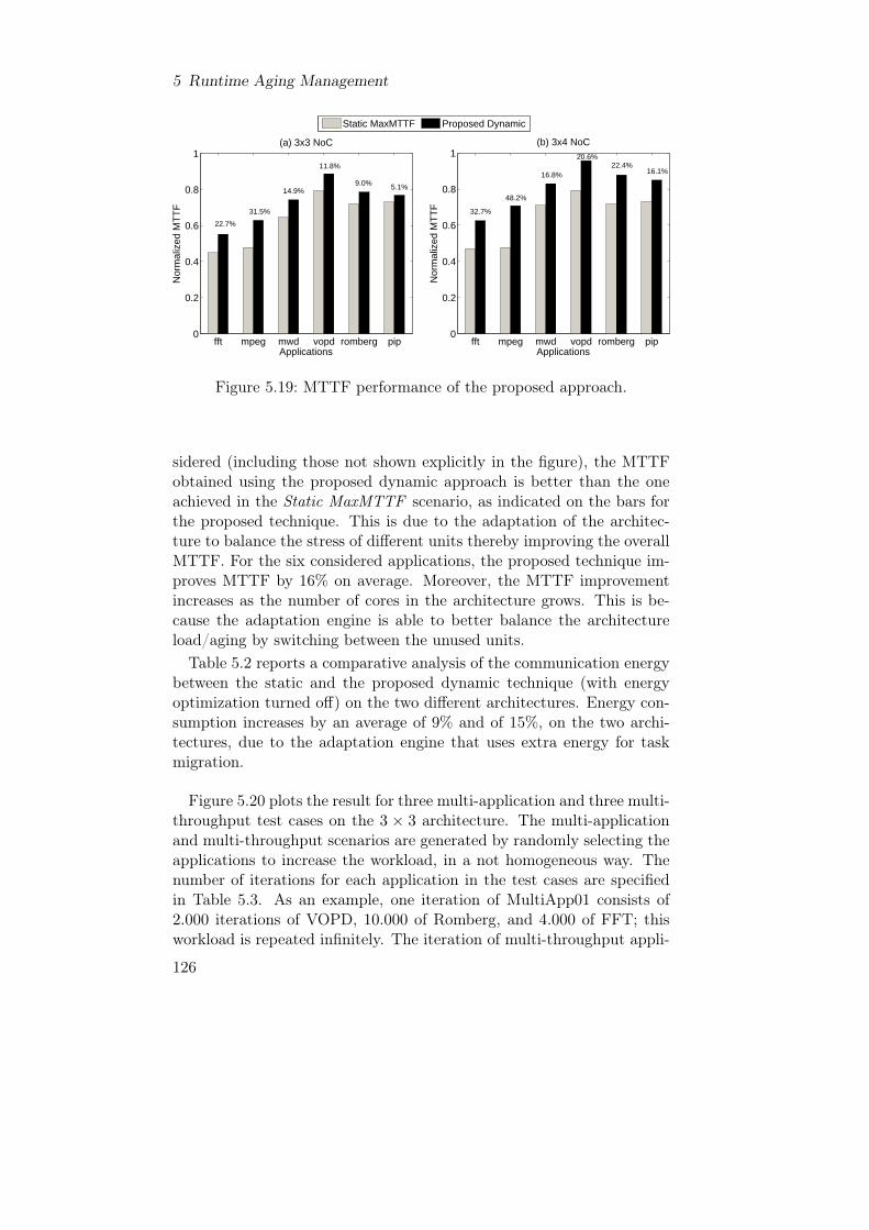
5 Runtime Aging Management
fft mpeg mwd vopd romberg pip0
0.2
0.4
0.6
0.8
1
Applications
Nor
mal
ized
MT
TF
(a) 3x3 NoC
fft mpeg mwd vopd romberg pip0
0.2
0.4
0.6
0.8
1
Applications
Nor
mal
ized
MT
TF
(b) 3x4 NoC
Static MaxMTTF Proposed Dynamic
31.5%
14.9%
11.8%
9.0% 5.1%
22.7%
32.7%
48.2%
16.8%22.4%
16.1%
20.6%
Figure 5.19: MTTF performance of the proposed approach.
sidered (including those not shown explicitly in the figure), the MTTFobtained using the proposed dynamic approach is better than the oneachieved in the Static MaxMTTF scenario, as indicated on the bars forthe proposed technique. This is due to the adaptation of the architec-ture to balance the stress of different units thereby improving the overallMTTF. For the six considered applications, the proposed technique im-proves MTTF by 16% on average. Moreover, the MTTF improvementincreases as the number of cores in the architecture grows. This is be-cause the adaptation engine is able to better balance the architectureload/aging by switching between the unused units.Table 5.2 reports a comparative analysis of the communication energy
between the static and the proposed dynamic technique (with energyoptimization turned off) on the two different architectures. Energy con-sumption increases by an average of 9% and of 15%, on the two archi-tectures, due to the adaptation engine that uses extra energy for taskmigration.
Figure 5.20 plots the result for three multi-application and three multi-throughput test cases on the 3 × 3 architecture. The multi-applicationand multi-throughput scenarios are generated by randomly selecting theapplications to increase the workload, in a not homogeneous way. Thenumber of iterations for each application in the test cases are specifiedin Table 5.3. As an example, one iteration of MultiApp01 consists of2.000 iterations of VOPD, 10.000 of Romberg, and 4.000 of FFT; thisworkload is repeated infinitely. The iteration of multi-throughput appli-
126

5.3 Aging Mitigation through Self-Adaptiveness
Applications Static MaxMTTF Proposed Dynamic3× 3 3× 4
FFT 1 1 1.162704082MPEG 1 1.017674265 1MWD 1 1.040284091 1VOPD 1 1.138318841 1.286558603
Romberg 1 1 1.052919355PiP 1 1.346435185 1.430726496
Average 1 1.090452064 1.155484756
Table 5.2: Energy performance of the proposed dynamic approach withMTTF optimization only
MultiApp01 MultiApp02 MultiApp03
VOPD (2,000) MPEG (5,000) MPEG (10,000)Romberg (10,000) MPEG (1,000) PiP (5,000)
FFT (4,000) Romberg (4,000) VOPD (4000)MPEG (1,000) PiP (8,000)
MultiThr01 MultiThr02 MultiThr03
MPEG1 (10,000) VOPD1 (10,000) PiP1 (10,000)MPEG2 (10,000) VOPD2 (10,000) PiP2 (10,000)
Table 5.3: Parameters for multi-application and multi-throughput
cation MultiThr01 consists of 10.000 iterations of MPEG with the samedeadline used in the static scenario, and 10.000 iterations with deadlinerelaxed by 2×.The static approach generates application mappings considering an
unused architecture, i.e., age of all the nodes are 0. As a result, whenapplications are switched at run-time, the static pre-computed mappingsare no-longer optimal in terms of MTTF because they ignore the cur-rent age of the different cores. Such information, on the other hand,is exploited by the dynamic approach that can adapt accordingly andproduce MTTF optimized solutions. For all the three multi-applicationsconsidered, the proposed technique improves the architecture MTTF by27% on average.Applications are often characterized by varying throughput require-
127

5 Runtime Aging Management
MultiApp01 MultiApp02 MultiApp03 MultiThr01 MultiThr02 MultiThr030
0.2
0.4
0.6
0.8
1
Nor
mal
ized
MT
TF
Static MTTFProposed Dynamic
Figure 5.20: MTTF performance with multi-application and multi-throughput scenarios.
ments. Computing the application mapping at design-time for all ap-plications and for all throughput requirements results in an explosionin the design space. With 20 applications having on average two dif-ferent throughput requirements, the number of application mappingsto be pre-computed at design-time is 220. This imposes a significantoverhead in terms of storage for the mapping, and of time to retrievethe information at runtime. An alternative approach adopted for mostdesign-time approaches is to generate one mapping for each of these ap-plications by using the stricter throughput requirement. Therefore, suchapproach gives good results when the throughput requirement is strict,but is not able to optimize the MTTF when the requirement is relaxed.Indeed, the dynamic approach is able to adapt to this changing scenario.Although, the initial mapping for the dynamic approach is the one pre-computed at design-time with a stricter deadline, the adaptive engine isable to explore different other mappings fulfilling the relaxed through-put requirement, possibly achieving better results. Experimental resultsfor the three multi-throughput applications indicate that the proposedtechnique improves system MTTF by 22%, on average, when comparedto the one using static mapping without adaptation.
Figure 5.21 plots the normalized communication energy of the pro-posed technique compared to the static approach, when optimizing bothcommunication energy and MTTF. Similarly to the previous experi-ments, the initial mapping for this experiment is the best MTTF map-ping coming from the static approach. However, the orchestrator in-corporates communication energy and system lifetime when selecting alocal move. For a more comprehensive comparison, we report results withand without the communication energy optimization, to highlight how
128

5.3 Aging Mitigation through Self-Adaptiveness
Proposed DynamicProposed Dynamic with Energy Optimization
Static MaxMTTF
Nor
mal
ized
Com
m. E
nerg
y
0
0.5
1.0
1.5
Nor
mal
ized
MTT
F
0.5
1.0
1.5
fft mpeg mwd vopd romberg pip
Figure 5.21: Communication energy performance for the proposedtechnique.
MTTF and energy consumption are affected. All values are normalizedwith respect to the data obtained using the static approach. As it can beseen, MTTF-communication energy joint optimization results in energysavings between 25% to 75% for all the applications considered with anaverage 5% MTTF improvement. Thus by trading-off MTTF, the com-munication energy can be minimized by 50%, if considering the averageof the results obtained on the considered benchmark applications.
5.3.4 Putting it all together
The last step in optimizing the lifetime/energy consumption trade-off isto consider communication and computation energy together in a multi-node architecture.
Each node has a ARM big.LITTLE architecture and the nodes are con-nected through a NoC communication infrastructure (both these aspectsare relevant in this case). Applications are modeled as fork-join task-graphs and not as serial applications, since data exchange among tasksis fundamental for evaluating communication energy consumption. Per-formance constraints are considered both in terms of worst case heartrateand a deadline not to be missed. The communication energy model is thesame as the ones presented in Section 5.3.3, while computation energyconsumption is modeled as described in Section 5.3.2. In particular, thecommunication energy consumption will be considered for the NoC only,neglecting internal contributions, since bus-based architectures usually
129

5 Runtime Aging Management
consume way less energy than NoC-based ones, since they consist offewer elements and do not have links and routers to be powered-up [97].
Orchestrator Design
At the multi-node level, the orchestrator behavior is inspired by the hy-brid technique described in Section 5.3.3, where good mapping solutionscomputed at design-time are optimized at runtime. The same state-of-artstatic strategy [36] has been exploited for computing such design time so-lutions. It performs an accurate design space exploration by consideringthe information available at design-time (the applications task-graphs,the architecture topology, and the performance constraint). The factthat computation energy is not considered during the design space ex-ploration does not represents a limitation, since at this level all the nodesare homogeneous and, at time 0, they share the same initial status. Com-putation energy optimization is considered in the runtime phase of thearchitecture, where the mappings retrieved from the database are opti-mized. Algorithm 4 has been modified in order to keep into considerationcomputation energy consumption as well when sorting the selected moves(Line 9); the score of each move is computed as in Algorithm 4 by con-sidering an aging contribution and an energy one, where the latter oneconsiders both communication and computation energy, in particular:
∆Etj ,Cni = α ·∆CompEtj ,Cni + β ·∆CommEtj ,Cni = (5.17)
= α · (CompEref − CompEmove) + β · (CommEref − CommEmove)(5.18)
where α and β are weighting coefficients and CommEref , CommEmovehave the same meaning as CEref and CEmove in Algorithm 4, respec-tively, while CompEref refers to the computation energy consumption ofthe current solution and CompEmove to the one of the move under test.In this way, moves resulting in an increase of energy consumption willreceive a negative score, placing them at the end of the list, while moveswith the highest energy saving will be at the top. The orchestrator canfind mappings characterized by a low computation energy consumptionat runtime by exploiting, for example, already powered on clusters orby grouping on the same node tasks requiring the same performancelevel. As in the inspiring approach, the orchestrator needs to evaluatethe make-span due to the new mapping by actually running the systemfor one cycle. In case the make-span for the current move is lower thanthe deadline, the move is accepted and the orchestrator will remain in-active until the activation condition will be triggered another time. If
130

5.3 Aging Mitigation through Self-Adaptiveness
Mapping Database Performance
Ener
gy
Constraints &Run-Time Metrics
Reliability
Performance
Energy Consumption
Constraints & Design-Time
Metrics
ArchitectureSet of Applications
Performance
Reliability
Performance
Relia
bilit
y
Performance
Relia
bilit
y
DVFSController
big
LITTLE
AgeBalancer
HelperDe
sign-
Tim
e Co
mpu
tatio
n
Run-
Tim
e O
ptim
izatio
n
Multi-node Intra-node
Figure 5.22: Overview of the proposed approach when both communica-tion and computation energy consumptions are optimized.
the make-span exceeds the deadline, the current move is discarded andthe next move in the sorted list is selected for evaluation, and so on.
It is worth noting that the coefficients α and β can be tuned to prop-erly weight the contributions of computation energy and communicationenergy in the moves score. α should be grater than β in computing-intensive scenarios; in case of high data exchange applications the rela-tionship between α and β will be the other way around. In particular,when α = 0 communication energy only is optimized at the multi-nodelevel and the approach leads back to the one described in Algorithm 4.On the other hand, when β = 0 computation energy only is consideredand an approach similar to the one proposed in Section 5.3.2 is obtained.
At the single node level, since communication energy is neglected, thesolution proposed in Section 5.3.1 has been exploited. Thus, an AgeBalancer and a DVFS Controller (together with its Helper) are imple-mented, per node, to manage the energy computation/lifetime reliabilitytrade-off. The proposed approach is summarized in Figure 5.22, wherethe runtime optimization box has been updated with reference to Fig-ure 5.18 and contains both a multi-node and an intra-node optimizationpolicy.
131

5 Runtime Aging Management
5.4 Final Remarks
This chapter presented a self-adaptive infrastructure for extending multi-/manycore architectures lifetime. First, an enabling tool was designedto make the lifetime estimation fast and precise. Then this tool wasexploited to evaluate the effectiveness of the implemented orchestrator,aiming at maximizing lifetime, while reducing energy consumption andmeeting performance constraints. To achieve this goal, the orchestratorhas to properly coordinate different components acting on the appli-cations mapping and scheduling, on the resources status and on theirworking voltage-frequency points. The problem is faced gradually, con-sidering first a single node and computation energy only, then moving toa more complex architecture and to communication energy optimizationas well.
In the next chapter, the idea of designing a system exploiting boththe self-adaptive systems presented in this chapter and in the previousone will introduced and discussed. Moreover, some concluding remarksfor the whole work described in this thesis will be drawn, together withpossible future developments.
132

6 Conclusions & Future Works
The research presented in this thesis has proposed a novel self-adaptive,reliable framework for in multi/manycore architectures. The work ismotivated by the necessity of dynamically exploiting reliability/energyconsumption/performance trade-offs when considering highly evolvingworking scenarios. Runtime resource management solutions are to bedesigned to properly adapt the system’s behavior to the changing envi-ronment; this is the reason why classical design-time (static) approachesdo not suffice in providing satisfying result and the adoption of a newprotocol (the Observe-Decide-Act control loop) was needed.The objective of this research is to design a system with self-adaptive
capabilities, able to make smart decisions at runtime and get the mostout of the considered trade-offs. Reliability represents the main optimiza-tion dimension. Energy consumption minimization has been introducedbecause it is directly and considerably affected by the knobs the frame-work was exploiting. Perfomance has been considered as a constraintto be satisfied according to the soft real-time paradigm. The result is across-layer self-adaptive system for the combined optimization of relia-bility (treated both as fault management and components lifetime) andenergy consumption (both communication and computation one) underperformance constraints. The proposed framework autonomously takescare of the resource management problem, hiding its complexity and tak-ing its burden away from the programmer. The overall work is organizedin several layers as shown in Figure 6.1 and summarized in the following.At the multi-node level, the designed framework employs a hybrid ap-
proach to minimize aging while optimizing communication and computa-tion energy consumption (Layer A in Figure 6.1). A runtime orchestratorhas been designed to smartly map tasks on the available nodes startingfrom pre-computed optimal mappings. Tasks are then re-mapped, atruntime by means of heuristics, to cope with the evolving conditions (Sec-tion 5.3.4). Transient fault management is considered at the intra-nodelevel only, since creating, scheduling, and gathering results of redundantthreads and voters/checkers benefit from a shared-memory bus-basedarchitecture such as the intra-node one (Layer B in Figure 6.1). A rule-based system has been designed to guide the orchestrator in selecting,at each instant of time, the best redundancy-based reliable technique to
133

6 Conclusions & Future Works
Heterog
eneo
us Platf
ormAgin
g Mitig
ation &
Ene
rgy Con
sumptio
n
O
ptimiza
tion La
yer
ARM
big.LI
TTLE
big cluste
rLIT
TLE
c
luster
Multi-nodeLevel
Intra-nodeLevel
A
Aging M
itigatio
n &
Com
putat
ion Ene
rgy
O
ptimiza
tion La
yerC
Transie
nt Fau
lts
M
anag
emen
t Laye
rB
Figure 6.1: A graphical representation of the research contribution of thisthesis, organized in self-adaptive layers.
satisfy the user’s reliability requirements and minimize the perfomanceoverhead (Chapter 4). This layer is located, in each node, on top ofanother adaptation layer that takes care of aging mitigation and com-putation energy optimization (Layer C in Figure 6.1). This is achievedby acting on different knobs (tasks mapping and scheduling, resourceswitch-on/off, DVFS) through the synergic orchestration on ad-hoc de-signed controllers (Section 5.3.1). Each adaptive layer has been validatedin a simulation environment by executing application traces collectedfrom execution on real architectures. The obtained results proved theeffectiveness of the proposed approach, obtaining remarkable improve-ments in terms of lifetime extension and energy consumption reduction,while meeting performance constraints.The envisioned framework and the design of the presented adaptation
layers represent the main innovative contribution of this research work.The preliminary investigation on self-adaptive systems led to the formal-ization of a model for describing and organizing this kind of systems ina structured and systematic way, as well as for preliminary validatingthem. Moreover, the need for estimating complex architectures lifetimemotivated the development of a lightweight framework for MTTF esti-
134

mation, based on Monte Carlo simulations and random walks. Thesetopics, discussed in Chapter 3 and Section 5.2.3, respectively, representfurther contributions of this thesis.Although many aspect have been covered in this research work, some
others are yet to be explored. Thus, there are several directions for futurework; the more relevant ones are listed below.
Extend the proposed framework to consider process variability. Withtechnology scaling, core-to-core parameters variations pose a major chal-lenge to high-performance microprocessor design, negatively impactingcores frequency and leakage power [82], thus motivating the need forvariation-aware optimization algorithms to be integrated in the proposedframework. The literature on self-adaptive variability-aware approachesshould be surveyed (i.e., [38, 13]) and the possibility to integrate vari-ability management within the proposed framework investigated.
Further integration of the system components. A possible extensionof the various designed components is their integration in a unique re-source manager. This would allow to overcome an important disadvan-tage of the proposed layered adaptive system: an application cannot bemapped in more than one node due to the node-granularity solution oflayer B for transient faults. A mechanism to manage and coordinatearchitecture across nodes is to be design, in order not to limit the ap-plication parallelism. Moreover, the MTTF evaluation tool presentedin Section 5.2.3 could be used at runtime to make the decision mak-ing process even more aware, and not only for the off-line estimation.Last, the model for self-adaptive systems presented in Chapter 3 couldbe exploited in the system implementation phase, for the developmentof a framework able to generate, in a template-fashion, a stub of theorchestrator according to the driving dimensions value.
Exploration of new reliable techniques. The reliable scheduling tech-niques considered in Chapter 4 are all based on the idea of indiscrim-inately replicating all the tasks in a task-graph, even if with differentgranularities or a varying number of times. An interesting developmentis to consider scheduling techniques based on selective replication; ac-cording to this approach, only a given percentage of tasks in the elabo-ration phase is actually replicated. This idea can be applied only if therequired fault tolerance coverage is not 100%, but it allows to furtherexploit the reliability/performance trade-off.
135

6 Conclusions & Future Works
Improvement of the decision making process. The decision makingprocess was carried out mainly through heuristics and rule-based algo-rithms, which fail in providing any kind of guarantee about their con-vergence and the obtained system’s stability; the only exception is rep-resented by the DVFS controller that exploits a control theory-basedapproach. More advanced control theoretical approaches [72, 71], ma-chine learning algorithms [70] and even price theory-based techniques[88] proved their effectiveness in dealing with the resource managementproblem and the possibility to integrate them in the proposed frameworkshould be investigated.
136

Bibliography
[1] Accelera Systems Initiative. http://www.accellera.org.
[2] N. Aggarwal, P. Ranganathan, N. P Jouppi, and J. E. Smith.Configurable isolation: building high availability systems withcommodity multi-core processors. In International Symposium onComputer Architecture, pages 470–481, 2007.
[3] ARM Ltd. http://www.arm.com/products/tools/development-boards/versatile-express/index.php, 2011.
[4] M. Auslander, D. Dasilva, D. Edelsohn, O. Krieger, M. Ostrowski,B. Rosenburg, R.W. Wisniewski, and J. Xenidis. K42 overview.Technical report, IBM T. J. Watson Research Center, August 2002.
[5] P. Bailis, V. J. Reddi, S. Gandhi, D. Brooks, and M. Seltzer.Dimetrodon: Processor-level preventive thermal management viaidle cycle injection. In Design Automation Conference, pages 89–94, 2011.
[6] M. Baldauf, S. Dustdar, and F. Rosenberg. A survey on context-aware systems. International Journal on Ad Hoc and UbiquitousComputing, 2(4):263–277, 2007.
[7] A. Baumann, P. Barham, P.E. Dagand, T. Harris, R. Isaacs, S. Pe-ter, T. Roscoey, A. Schüpbach, and A. Singhania. The multikernel:a new OS architecture for scalable multicore systems. In Syposiumon Operating Systems Principles, pages 29–44, 2009.
[8] R.C. Baumann. Radiation-induced soft errors in advanced semi-conductor technologies. Transactions on Device and Materials Re-liability, 5(3):305–316, Sept 2005.
[9] T. Becker, A. Agne, P. R. Lewis, R. Bahsoon, F. Faniyi, L. Es-terle, A. Keller, A. Chandra, A. R. Jensenius, and S. C. Stilkerich.EPiCS: Engineering Proprioception in Computing Systems. In In-ternational Conference on Computational Science and Engineer-ing, pages 353–360, 2012.
137

Bibliography
[10] L. Benini and G. De Micheli. Networks on chips: A new socparadigm. IEEE Computer, 35(1):70–78, 2002.
[11] D. Bertozzi, A. Jalabert, S. Murali, R. Tamhankar, S. Stergiou,L. Benini, and G. De Micheli. Noc synthesis flow for customizeddomain specific multiprocessor systems-on-chip. Transactions onParallel and Distributed Systems, 16(2):113–129, 2005.
[12] L. Bin, P. Li-Shiuan, and P. Patra. Impact of process and temper-ature variations on network-on-chip design exploration. In Inter-national Symposium on Networks-on-Chip, pages 117–126, April2008.
[13] G. Bizot, F. Chaix, N.E. Zergainoh, and M. Nicolaidis. Variability-aware and fault-tolerant self-adaptive applications for many-corechips. In International On-Line Testing Symposium, pages 37–42,July 2013.
[14] G. Blake, R.G. Dreslinski, and T. Mudge. A survey of multicoreprocessors. Signal Processing Magazine, 26(6):26–37, November2009.
[15] J. Blome, F. Shuguang, S. Gupta, and S. Mahlke. Self-calibratingonline wearout detection. In International Symposium on Microar-chitecture, pages 109–122, Dec 2007.
[16] C. Bolchini and M. Carminati. Multi-core emulation for depend-able and adaptive systems prototyping. In Workshop on Manu-facturable and Dependable Multicore Architectures at Nanoscale,pages 1–4, March 2014.
[17] C. Bolchini, M. Carminati, M. Gribaudo, and A. Miele. Alightweight and open-source framework for the lifetime estimationof multicore systems. In International Conference on ComputerDesign, pages 1–7, October 2014.
[18] C. Bolchini, M. Carminati, and A. Miele. Towards the designof tunable dependable systems. In Workshop on Manufacturableand Dependable Multicore Architectures at Nanoscale, pages 17–21,June 2012.
[19] C. Bolchini, M. Carminati, and A. Miele. Self-adaptive fault toler-ance in multi-/many-core systems. Journal of Electronic Testing,29(2):159–175, 2013.
138

Bibliography
[20] C. Bolchini, M. Carminati, A. Miele, A. Das, A. Kumar, andB. Veeravalli. Run-time mapping for reliable many-cores basedon energy/performance trade-offs. In International Symposium onDefect and Fault Tolerance in VLSI and Nanotechnology Systems,pages 58–64, 2013.
[21] C. Bolchini, M. Carminati, A. Miele, and E. Quintarelli. A frame-work to model self-adaptive computing systems. In Conference onAdaptive Hardware and Systems, pages 71–78, 2013.
[22] C. Bolchini, M. Carminati, T. Mitra, and T. Somu Muthukarup-pan. Combined on-line lifetime-energy optimization for asymmetricmulticores. In Technical Report, 2014.
[23] C. Bolchini, C. Curino, E. Quintarelli, F. A. Schreiber, andL. Tanca. Context information for knowledge reshaping. Inter-national Journal of Web Engineering and Technology, 5(1):88–103,2009.
[24] C. Bolchini, A. Miele, and C. Sandionigi. A novel design method-ology for implementing reliability-aware systems on SRAM-basedFPGAs. Transactions on Computers, 60(12):1744–1758, 2011.
[25] C. Bolchini, A. Miele, and D. Sciuto. An adaptive approach foronline fault management in many-core architectures. In Conferenceon Design, Automation Test in Europe, pages 1429–1432, March2012.
[26] S. Borkar, T. Karnik, and V. De. Design and reliability chal-lenges in nanometer technologies. In Design Automation Confer-ence, pages 75–75, 2004.
[27] E. Carvalho, N. Calazans, and F. Moraes. Heuristics for dynamictask mapping in NoC-based heterogeneous MPSoCs. In Interna-tional Workshop on Rapid System Prototyping, pages 34–40, 2007.
[28] T. Chantem, R. P. Dick, and X. S. Hu. Temperature-aware schedul-ing and assignment for hard real-time applicationson MPSoCs. InConference on Design, Automation and Test in Europe, pages 288–293, 2008.
[29] T. Chantem, Y. Xiang, X.S. Hu, and R.P. Dick. Enhancing mul-ticore reliability through wear compensation in online assignmentand scheduling. In Conference on Design, Automation and Test inEurope, pages 1–6, 2013.
139

Bibliography
[30] Z. Chen, M. Yang, G. Francia, and J. Dongarra. Self adaptiveapplication level fault tolerance for parallel and distributed com-puting. In International Symposium on Parallel and DistributedProcessing, pages 1–8, 2007.
[31] C.L. Chou and R. Marculescu. FARM: Fault-aware resource man-agement in NoC-based multiprocessor platforms. In Conference onDesign, Automation Test in Europe, pages 1–6, 2011.
[32] S. Corbetta, D. Zoni, and W. Fornaciari. A temperature and reli-ability oriented simulation framework for multi-core architectures.In International Symposium on VLSI, pages 51–56, 2012.
[33] A.K. Coskun, T. Simunic, K. Mihic, G. De Micheli, andY. Leblebici. Analysis and optimization of MPSoC reliability. Jour-nal of Low Power Electronics, pages 56–69, 2006.
[34] A.K. Coskun, R. Strong, D.M. Tullsen, and T. Simunic Rosing.Evaluating the impact of job scheduling and power managementon processor lifetime for chip multiprocessors. In InternationalConference Measurement and Modeling Computer Systems, pages169–180, 2009.
[35] A. Das, A. Kumar, and B. Veeravalli. Communication and mi-gration energy aware task mapping for reliable multiprocessor sys-tems. Future Generation Computer Systems, 2013.
[36] A. Das, A. Kumar, and B. Veeravalli. Reliability-driven task map-ping for lifetime extension of networks-on-chip based multiproces-sor systems. In Conference on Design, Automation and Test inEurope, pages 689–694, 2013.
[37] A. Das, A. Kumar, and B. Veeravalli. Temperature aware energy-reliability trade-offs for mapping of throughput-constrained appli-cations on multimedia MPSoCs. In Conference on Design, Au-tomation and Test in Europe, pages 1–6, 2014.
[38] S. Dighe, S.R. Vangal, P. Aseron, S. Kumar, T. Jacob, K.A.Bowman, J. Howard, J. Tschanz, V. Erraguntla, N. Borkar, V.K.De, and S. Borkar. Within-die variation-aware dynamic-voltage-frequency-scaling with optimal core allocation and thread hoppingfor the 80-core teraflops processor. Journal of Solid-State Circuits,46(1):184–193, Jan 2011.
140

Bibliography
[39] E. Fernandez-Alonso, D. Castells-Rufas, J. Joven, and J. Carra-bina. Survey of NoC and programming models proposals for MP-SoC. International Journal of Computer Science Issues, 9(2):22–32, 2012.
[40] European Cooperation for Space Standardization. Methods for thecalculation of radiation received and its effects, and a policy fordesign margins. Technical Report ECSS-E-ST-10-12C, November2008.
[41] D. Gizopoulos, M. Psarakis, S.V. Adve, P. Ramachandran, S.K.S.Hari, D. Sorin, A. Meixner, A. Biswas, and X. Vera. Architecturesfor Online Error Detection and Recovery in Multicore Processors.In Conference on Design, Automation and Test in Europe, pages533–538, 2011.
[42] Z. Gu, C. Zhu, L. Shang, and R. P. Dick. Application-specificMPSoC reliability optimization. Transactions on VLSI Systems,16(5):603–608, 2008.
[43] A.S. Hartman and D.E. Thomas. Lifetime improvement throughruntime wear-based task mapping. In International Conferenceon Hardware/software codesign and system synthesis, pages 13–22,2012.
[44] K. Henricksen and J. Indulska. A software engineering frameworkfor context-aware pervasive computing. In Conference on PervasiveComputing and Communications, pages 77–86, 2004.
[45] H. Hoffmann, J. Eastep, M.D. Santambrogio, J.E. Miller, andA. Agarwal. Application heartbeats: A generic interface for spec-ifying program performance and goals in autonomous computingenvironments. In International Conference on Autonomic Com-puting, pages 79–88, 2010.
[46] P. Horn. Autonomic Computing: IBM’s Perspective on the Stateof Information Technology, 2001.
[47] Y. Hoskote, S. Vangal, A. Singh, N. Borkar, and S. S. Borkar. A5-ghz mesh interconnect for a teraflops processor. Micro, IEEE,27(5):51–61, Sept 2007.
[48] J. Hu and R. Marculescu. Energy-aware communication and taskscheduling for network-on-chip architectures under real-time con-straints. In Conference on Design, Automation and Test in Europe,pages 234–239, 2004.
141

Bibliography
[49] J. Huang, J.O. Blech, A. Raabe, C. Buckl, and A. Knoll. Analy-sis and optimization of fault-tolerant task scheduling on multipro-cessor embedded systems. In International Conference on Hard-ware/software codesign and system synthesis, pages 247–256, 2011.
[50] L. Huang and Q. Xu. AgeSim: A simulation framework for evaluat-ing the lifetime reliability of processor-based SoCs. In Conferenceon Design, Automation and Test in Europe, pages 51–56, 2010.
[51] L. Huang and Q. Xu. Lifetime reliability for load-sharing redun-dant systems with arbitrary failure distributions. Transactions onReliability, 59(2):319–330, 2010.
[52] L. Huang, R. Ye, and Q. Xu. Customer-aware task allocationand scheduling for multi-mode MPSoCs. In Design AutomationConference, pages 387–392, 2011.
[53] L. Huang, F. Yuan, and Q. Xu. Lifetime reliability-aware taskallocation and scheduling for MPSoC platforms. In Conference onDesign, Automation and Test in Europe, pages 51–56, 2009.
[54] L. Huang, F. Yuan, and Q. Xu. On task allocation and schedulingfor lifetime extension of platform-based MPSoC designs. Transac-tions on Parallel and Distributed Systems, 22(12):2088–2099, 2011.
[55] International Technology Roadmap for Semiconductors – Emerg-ing Research Devices Section. http://public.itrs.net/, 2010.
[56] A. Jantsch and H. Tenhunen. Will networks on chip close theproductivity gap? In Networks on Chip, pages 3–18. Springer US,2003.
[57] JEDEC Solid State Technology Association and others. Failuremechanisms and models for semiconductor devices. JEDEC Pub-lication JEP122G, 2010.
[58] E. Karl, D. Blaauw, D. Sylvester, and T. Mudge. Multi-mechanismreliability modeling and management in dynamic systems. Trans-actions on VLSI Systems, 16(4):476–487, 2008.
[59] K.M. Kavi, R. Giorgi, and J. Arul. Scheduled dataflow: executionparadigm, architecture, and performance evaluation. Transactionson Computers, 50(8):834–846, 2001.
[60] J.O. Kephart and D.M. Chess. The vision of autonomic computing.Computer, 36:41–50, 2003.
142
Bibliography
[61] I. Koren and C.M. Krishna. Fault-Tolerant Systems. Elsevier Sci-ence, 2010.
[62] A. Kouadri, O. Heron, and R. Montagne. A lightweight API foran adaptive software fault tolerance using POSIX-thread replica-tion. In International Conference on Architecture of ComputingSystems, pages 16–19, 2011.
[63] Y.K. Kwok and I. Ahmad. Static scheduling algorithms for allocat-ing directed task graphs to multiprocessors. Computing Surveys,31(4):406–471, 1999.
[64] C. Kyriacou, P. Evripidou, and P. Trancoso. Data-driven mul-tithreading using conventional microprocessors. Transactions onParallel and Distributed Systems, 17(10):1176–1188, 2006.
[65] C. LaFrieda, E. Ipek, J. F. Martinez, and R. Manohar. Utilizingdynamically coupled cores to form a resilient chip multiprocessor.In Conference on Dependable Systems and Networks, pages 317–326, 2007.
[66] J.C. Laprie. Dependable computing: Concepts, limits, challenges.In International Conference on Fault-tolerant Computing, pages42–54, 1995.
[67] M. Lattuada, C. Pilato, A. Tumeo, and F. Ferrandi. Performancemodeling of parallel applications on MPSoCs. In InternationalConference on System-on-Chip, pages 64–67, 2009.
[68] Linaro Ubuntu release for Vexpress. http://releases.linaro.org, 2014.
[69] H. Liu. Reliability of a load-sharing k-out-of-n:G system: non-iidcomponents with arbitrary distributions. Transactions on Relia-bility, 47(3):279–284, 1998.
[70] M. Maggio, H. Hoffmann, A.V. Papadopoulos, J. Panerati, M.D.Santambrogio, A. Agarwal, and A. Leva. Comparison of decision-making strategies for self-optimization in autonomic computingsystems. Transactions on Autonomous and Adaptive Systems,7(4):36:1–36:32, 2012.
[71] M. Maggio, H. Hoffmann, M.D. Santambrogio, A. Agarwal, andA. Leva. Power optimization in embedded systems via feedbackcontrol of resource allocation. Transactions on Control SystemsTechnology, 21(1):239–246, Jan 2013.
143

Bibliography
[72] M. Maggio, F. Terraneo, and A. Leva. Task scheduling: A control-theoretical viewpoint for a general and flexible solution. Transac-tions on Embedded Computing Systems, 13(4):76:1–76:22, 2014.
[73] P. Meloni, G. Tuveri, L. Raffo, E. Cannella, T. Stefanov, O. Derin,L. Fiorin, and M. Sami. System adaptivity and fault-tolerance inNoC-based MPSoCs: the MADNESS project approach. In Con-ference on Digital System Design, pages 517–524, 2012.
[74] P. Mercati, A. Bartolini, F. Paterna, T.S. Rosing, and L. Benini.Workload and user experience-aware dynamic reliability manage-ment in multicore processors. In Design Automation Conference,pages 2:1–2:6, 2013.
[75] S.S. Mukherjee, M. Kontz, and S.K. Reinhardt. Detailed designand evaluation of redundant multi-threading alternatives. In In-ternational Symposium on Computer Architecture, pages 99–110,2002.
[76] H.V. Nguyen. Multilevel Interconnect Reliability: On the Effectsof Electro-Thermomechanical Stresses. PhD thesis, University ofTwente, Twente, Netherland, 2004.
[77] E. Normand. Single event upset at ground level. Transactions onNuclear Science, 43(6):2742–2750, 1996.
[78] NVidia Corporation. The benefits of multi-ple cpu cores in mobile devices., 2011. http://www.nvidia.com/content/PDF/tegra_white_papers/Benefits-of-Multi-core-CPUs-in-Mobile-Devices_Ver1.2.pdf.
[79] J. Panerati, M. Maggio, M. Carminati, F. Sironi, M. Triverio, andM.D. Santambrogio. Coordination of independent loops in self-adaptive systems. Transactions on Reconfigurable Technology andSystems, 7(2):12:1–12:16, 2014.
[80] Politecnico di Milano. ReSP web site: http://code.google.com/p/resp-sim/, 2011.
[81] E.T. Salehi, M. Asadi, and S. Eryilmaz. Reliability analysis ofconsecutive k-out-of-n systems with non-identical components life-times. Journal of Statistical Planning and Inference, 141(8):2920–2932, 2011.
144

Bibliography
[82] S.R. Sarangi, B. Greskamp, R. Teodorescu, J. Nakano, A. Tiwari,and J. Torrellas. Varius: A model of process variation and resultingtiming errors for microarchitects. Transactions on SemiconductorManufacturing, 21(1):3–13, Feb 2008.
[83] B. Schilit, N. Adams, and R. Want. Context-aware computingapplications. In Workshop on Mobile Computing Systems and Ap-plications, pages 85–90, 1994.
[84] A. Sharifi, S. Srikantaiah, A. K. Mishra, M. Kandemir, and C. R.Chita. METE: meeting end-to-end QoS in multicores throughsystem-wide resource management. In International Conferenceon Measurement and modeling of computer systems, pages 13–24,2011.
[85] A. Shye, B. Scholbrock, and Gokhan G. Memik. Into the wild:studying real user activity patterns to guide power optimizationsfor mobile architectures. In International Symposium on Microar-chitecture, pages 168–178, 2009.
[86] F. Sironi, D. B. Bartolini, S. Campanoni, F. Cancare, H. Hoffmann,D. Sciuto, and M. D. Santambrogio. Metronome: operating systemlevel performance management via self-adaptive computing. InDesign Automation Conference, pages 856–865, 2012.
[87] K. Skadron, M.R. Stan, K. Sankaranarayanan, W. Huang,S. Velusamy, and D. Tarjan. Temperature-aware microarchitec-ture: Modeling and implementation. Transactions on ArchitectureCode Optimization, 1(1):94–125, 2004.
[88] T. Somu Muthukaruppan, A. Pathania, and T. Mitra. Price the-ory based power management for heterogeneous multi-cores. In In-ternational Conference on Architectural Support for ProgrammingLanguages and Operating Systems, pages 161–176, 2014.
[89] T. Somu Muthukaruppan, M. Pricopi, V. Venkataramani, T. Mi-tra, and S. Vishin. Hierarchical power management for asymmetricmulti-core in dark silicon era. In Design Automation Conference,pages 174:1–174:9, 2013.
[90] J. Srinivasan, S.V. Adve, P. Bose, and J.A. Rivers. The case forlifetime reliability-aware microprocessors. In International Sympo-sium on Computer Architecture, pages 276–287, 2004.
145

Bibliography
[91] S. Srinivasan and N.K. Jha. Safety and reliability driven taskallocation in distributed systems. Transactions on Parallel andDistributed Systems, 10(3):238–251, 1999.
[92] K. Stavrou, D. Pavlou, M. Nikolaides, P. Petrides, P. Evripidou,P. Trancoso, Z. Popovic, and R. Giorgi. Programming abstractionsand toolchain for dataflow multithreading architectures. In Inter-national Symposium on Parallel and Distributed Computing, pages107–114, 2009.
[93] STMicroelectronics and CEA. Platform 2012: A many-core pro-grammable accelerator for Ultra-Efficient Embedded Computingin Nanometer Technology. In Research Workshop on STMicroelec-tronics Platform 2012, 2010.
[94] Teraflux. Definition of ISA extensions, custom devices and Ex-ternal COTSon API extensions. In Teraflux: Exploiting dataflowparallelism in Tera-device Computing, 2011.
[95] The OpenMP API specification for parallel programming. http://openmp.org/wp/, 2011.
[96] L. Thiele, L. Schor, Y. Hoeseok, and I. Bacivarov. Thermal-aware system analysis and software synthesis for embedded multi-processors. In Design Automation Conference, pages 268–273,2011.
[97] A.N. Udipi, N. Muralimanohar, and R. Balasubramonian. Towardsscalable, energy-efficient, bus-based on-chip networks. In Interna-tional Symposium on High Performance Computer Architecture,pages 1–12, Jan 2010.
[98] Various Authors. The MIT Angstrom Project: Universal Tech-nologies for Exascale Computing - http://projects.csail.mit.edu/angstrom/index.html, 2011.
[99] P. M. Wells, K. Chakraborty, and G. S. Sohi. Mixed-mode multi-core reliability. In International Conference on Architectural Sup-port for Programming Languages and Operating Systems, pages169–180, 2009.
[100] M. Wirthlin, E. Johnson, N. Rollins, M. Caffrey, and P. Gra-ham. The reliability of FPGA circuit designs in the presence ofradiation induced configuration upsets. In Symposium on Field-Programmable Custom Computing Machines, pages 133–142, 2003.
146

Bibliography
[101] Y. Xiang, T. Chantem, R.P. Dick, X.S. Hu, and L. Shang. System-level reliability modeling for MPSoCs. In International Conferenceon Hardware/Software Codesign and System Synthesis, pages 297–306, 2010.
[102] T.T. Ye, L. Benini, and G. De Micheli. Packetized on-chip in-terconnect communication analysis for MPSoC. In Conference onDesign, Automation and Test in Europe, pages 344–349, 2003.
[103] W. Zhao and Y. Cao. Predictive technology model for nano-CMOSdesign exploration. Journal on Emerging Technologies in Comput-ing Systems, 3(1):1–17, 2007.
147