Towardsaself-consistent plate mantle model that … · Towardsaself-consistent plate mantle model that ... Maxwell model that explains many of the difﬁculties he has strug-

Geophys. J. Int. (2005) 163, 788–800 doi: 10.1111/j.1365-246X.2005.02742.xG

JITec

toni

csan

dge

ody

nam

ics

Towards a self-consistent plate mantle model that includes elasticity:simple benchmarks and application to basic modes of convection

Hans-Bernd Muhlhaus1,2 and Klaus Regenauer-Lieb2

1ESSCC, The University of Queensland, St Lucia, QLD 4072, Australia. E-mail: [email protected] Division of Exploration and Mining, 26 Dick Perry Ave., Kensington WA 6051, Australia

Accepted 2005 July 21. Received 2005 July 12; in original form 2005 January 25

S U M M A R YOne of the difficulties with self-consistent plate-mantle models capturing multiple physicalfeatures, such as elasticity, non-Newtonian flow properties and temperature dependence, is thatthe individual behaviours cannot be considered in isolation. For instance, if a viscous mantleconvection model is generalized naively to include hypo-elasticity, then problems based onEarth-like Rayleigh numbers exhibit almost insurmountable numerical stability issues due tospurious softening associated with the co-rotational stress terms. If a stress limiter is introducedin the form of a power-law rheology or yield criterion these difficulties can be avoided. In thispaper, a novel Eulerian finite element formulation for viscoelastic convection is presented andthe implementation of the co-rotational stress terms is addressed. The salient dimensionlessnumbers of viscoelastic–plastic flows such as Weissenberg, Deborah and Bingham numbersare discussed in a separate section in the context of Geodynamics. We present an Eulerianformulation for slow temperature-dependent, viscoelastic–plastic flows. A consistent tangent(incremental) formulation of the governing equations is derived. Numerical and analyticalsolutions demonstrating the effect of viscoelasticity, co-rotational terms are first discussed forsimplified benchmark problems. For flow around cylinders we identify parameter ranges ofpredominantly viscous and viscoplastic and transient behaviour. The influence of locally highstrain rates on the importance of elasticity and non-Newtonian effects is also discussed in thiscontext. For the case of simple shear we investigate in detail the effect of different co-rotationalstress rates and the effect of power-law creep. The results show that the effect of the co-rotationalterms is insignificant if realistic stress levels are considered (e.g. deviatoric invariant smallerthan 1/10 of the shear modulus say). We also consider the basic convection modes of stagnantlid, episodic resurfacing and mobile lid convection as applicable to a cooling planet. Thesimulations show that elasticity does not have a significant effect on global parameters suchas the Nusselt number and the qualitative nature of the basic convection pattern. Our simplebenchmarks show, however, also that elasticity plays a significant role for instabilities on thelocal scale of an individual subduction zone.

Key words: Visco-elasticity, plasticity, convection, Deborah number, co-rotational.

I N T RO D U C T I O N

Realistic simulations of earth processes such as faulting, shearing,magma flow, subduction and convection often require the consid-eration of non-Newtonian effects such as elasticity and power-lawcreep. Non-Newtonian effects combined in a single constitutive re-lationship allow, at least in principle, the modelling of key aspectsof planetary behaviour, such as mantle convection, the emergenceof an elastic or elasto-plastic boundary layer and even plate tec-tonics in a unified manner. Such models are unified in the sensethat different modes of mechanical behaviour are represented ascoincident features of a single physical model. Within a planet, thedifferent convection modes are controlled by the usually strong tem-

perature and pressure dependence of the coefficients of the viscouspart of the model. The existing models of mantle convection withemergent plate tectonics, for example,], often concentrate on twokey ingredients, namely the exponential dependence on the tem-perature of the viscosity (Arrhenius law) and a stress limiter in theform of a fracture, yield or damage criterion for example, Bercovici(1993), Solomatov (1995), Moresi & Solomatov (1998), Trompert& Hansen (1998), Ogawa (2003) and Tackley (1998, 2000a). Thereare but few papers in which the influence of elasticity is consid-ered. In the past, strongly viscoelastic convection simulations witha lithospheric component have been limited to models with explicitlayering in which a non-convecting viscoelastic layer is coupled to aviscous, convecting substratum (Poliakov et al. 1996). Viscoelastic

788 C© 2005 The Authors

Journal compilation C© 2005 RAS

Towards a self-consistent plate mantle model that includes elasticity 789

mantle convection has been limited to considering constant viscosity(Harder 1991). Harder’s derivations are based on an upper convectedMaxwell model that explains many of the difficulties he has strug-gled with: Maxwell models exhibit spurious strain softening andinstabilities at elevated stresses. These ‘side effects’ recede signifi-cantly as soon as a yield criterion or a stress limiter such as power-lawcreep is considered. These issues will be discussed in the followingsections. Models of subduction zones that incorporate viscoelastic-ity, faulting, and free surface behaviour have generally been limitedto modest evolution times, after which further deformation producessevere remeshing problems (Melosh 1978; Gurnis et al. 1996), orseparate the computational domains into a solid-mechanical do-main where elasticity is considered (cold slab) and a fluid-dynamicdomain (outer boundary of the slab) where elasticity is neglected(Regenauer-Lieb et al. 2001; Funiciello et al. 2003; Morra et al.2004). However, these approaches cannot produce self-consistentplate tectonics emerging out of mantle convection. Although signif-icant progress has been achieved by acknowledging non-Newtonianeffects in fluid mechanical approaches, achieving basic plate-likefeatures, spreading ridges and Earth-like toroidal/poloidal ratios(Tackley 2000a,b), it has been impossible to reproduce terrestrialsubduction zones. Subduction zones appear as vertical two-sideddownwellings. Comparatively, viscoelasto–plastic calculations pro-duce asymmetric subduction zones (Regenauer-Lieb et al. 2001)suggesting that elasticity is required to produce consistent models.Recent results (Regenauer-Lieb & Yuen 2004) have shown that sym-metry breaking in faulting arises as a result of elastic stored energyin a dissipative viscoelastic–plastic system.

In this context, an approach has been put forward by Moresi et al.(2002) where a novel finite element based on a moving integrationpoint scheme is applied to the simulation of mantle convection basedon temperature-dependent viscosity, Maxwell-type viscoelasticityand a pressure-dependant yield criterion. The latter acts as a stresslimiter thus avoiding spurious softening effects otherwise associatedwith viscoelasticity. However the main purpose of Moresi et al.’s(2002) paper was the illustration of the applicability of the modeland the Lagrangian integration point code in terms of a range ofsimple benchmark problems including a specific mantle convectionstudy.

This paper presents an alternative and more general fully Eulerianmodel applicable to a wide range of existing fluid dynamic models.The approach considers combined Newtonian and power-law creepas well as elasticity and temperature dependence of the creep param-eters. As the deformations involved in geological deformation arelarge the constitutive relationships must contain geometric terms en-suring that the tensor properties of the model are conserved. A modelwith such properties is described as being ‘objective’. There exist awide range of objective, viscoelastic–plastic models to choose from.The primary difference between these models consists in the choiceof the objective stress rate, such as Jaumann, Oldroyd or Truesdellrates (see Kolymbas & Herle 2003, for a recent discussion). In thefollowing we give an outline of the constitutive model, derive anincremental form for the constitutive operator and compare differ-ent models of viscoelasticity. The salient features of incompress-ible flows can be studied in homogeneous simple and pure shearflows, respectively (Appendix A1). For simple shear flow we com-pare the shear stress–shear strain curves for a constant applied shearstrain rate, assuming an infinitesimal deformation model (i.e. noco-rotational stress terms), Jaumann and Naghdi models, respec-tively. Subsequently we consider the problem of incompressible flowaround circular cylinders and highlight parameter ranges governedby viscous, viscoplastic and viscoelastic–plastic behaviour. Finally

we explore the behaviour of the model in a study on 2-D (planestrain) natural convection in one by one and two by one domainsfor various ratios of the effective relaxation time to the thermal dif-fusion time (Deborah number), power-law exponents and Rayleighnumbers.

C O N S T I T U T I V E M O D E L S

We use Cartesian coordinates xi with i = 1, 2, 3; vi are the com-ponents of the velocity vector, partial differentiation with respectto xj or the time t is written as a subscribed comma followed bythe index of the coordinate with respect to which we differentiate;for example, the velocity gradient L i j is defined as L i j = v i, j andaccordingly the partial time derivative of the velocity is written asv i,t ; σ i j are the components of the stress tensor, δ i j is the Kroneckerunit tensor, T is the temperature. The stretching Dij is defined asusual as the symmetric part of the velocity gradient L i j and the spinW i j = −W ji of an infinitesimal element of the continuum is givenby the anti-symmetric part of L i j .

In the formulation of the constitutive model we make the standardassumption that the stretching is the sum of an elastic, viscous anda plastic part, that is,

Di j = Dei j + Dv

i j + DPi j . (1)

For the elastic part we assume hypo-elasticity [see e.g. Prager1961 for the definition of elastic, hypo-elastic (constitutive equa-tions are in rate form; linear in the stretching) and hyper-elasticmaterials], for the viscous part we assume that the viscosity is madeup of a Newtonian and a power-law contribution (to be specifiedbelow) and for the plastic deformation we assume von Mises plas-ticity combined with the usual Prandtl–Reuss flow rule (Hill 1998);thus

Di j = 1

2µ˙σ

′i j + 1

2ησ ′

i j + γ Pσ ′

i j

2τ, Dkk = divv = 0, (2)

where the prime designates the deviator of each tensor; for example:

σ ′i j = σi j − 1

3σkkδi j . (3)

In the formulation of the equations we use index notationand adopt Einstein’s summation convention, that is, summationover equal indexes. The pressure is defined as usual as p =−1/3 trace σ i j . Incompressibility is also assumed since we aremainly interested in large deformations. The significance of theobjective or co-rotational stress rate ˙σ i j will be discussed in a sepa-rate section below. In eq. (2) the quantity τ is the second deviatoricstress invariant defined as τ =

√1/2σ ′

i jσ′i j and for later use we

define the equivalent strain rate as γ = √2Di j Di j ; µ and η are

the shear modulus and the shear viscosity, respectively. The shearviscosity is assumed in the form 1/η = 1/ηN + 1/η P , where 1/ηN

is the Newtonian viscosity and η P is the secant viscosity (instan-taneous viscosity derived from the secant in the stress–strain rateplot) of the power-law creep component. The power-law viscositydepends on the second deviatoric stress invariant and in addition,both viscosities may depend on the pressure and the temperature.Specific forms will be assumed below. Here we adopt the usualpractice in the earth science and assume that the shear modulus µ

is a constant. The coefficient of the last term in eq. (2) is the plasticmultiplier γ P . In the finite element simulations we shall assume avon Mises yield criterion with a constant yield stress τ Y , that is,τ ≤ τ Y . In classical rate-independent plasticity, γ P is determinedfrom the so-called consistency condition. Here we adopt a simple

C© 2005 The Authors, GJI, 163, 788–800


790 H.-B. Muhlhaus and K. Regenauer-Lieb

alternative to the rate-independent plasticity approach: we assumean evolution equation for γ P in the form γ P = τY /ηY (τ/τY )n pl ,where ηY is a reference viscosity and npl � 1 is the power-lawcoefficient of the plastic deformation. This approach is computa-tionally simpler than the conventional rate-independent plasticityapproach. In fact for constant yield stress and npl → ∞ the in-cremental constitutive equations of the power-law approach andthe plasticity approach coincide up to one detail: in the plastic-ity approach the consistency condition is satisfied by the materialstress derivative whereas in the power-law case it is the spatial stressderivative satisfies the consistency condition. See Appendix A2 fordetails.

The evolution equation for the equivalent strain rate for the power-law part of the stretching we notice that a vast number of experi-mental data of the flow properties by dislocation glide have beenfitted to power-law relationships of the type

γ vis P = γ0 exp(−ATM/T )

(τ

τ0

)n

, (4)

where γ0 and τ 0 are a reference strain rate and stress, respectively;A is the activation energy and TM is the melting temperature. In gen-eral, for dislocation creep or diffusion creep combined with stressdependence of the constitutive parameters such as grain size, n variesbetween 2 and 5. See Kirby (1983), and Karato & Wu (1993) forfurther details. A change in n of about unity is reported by someinvestigators at stresses less than 0.5 107–1.0 107 Pa. But overallthe value n = 3 seems to be a reasonable approximation for mostdislocation related geodynamic flows. The lower mantle seems tobe governed by diffusion type creep with linear stress dependenceof the stretching so that n = 1 in this case. We, therefore, adopt acombined rheology consisting of Newtonian and power-law creepcontributions (see also discussion below eq. (7). Stresses associatedwith convecting flow ranges from 106 Pa in the asthenosphere tolarger than 108 Pa in subducting plates. The high-stress regimes aregoverned largely by rate-independent or almost-rate-independentmaterial behaviour, elasticity and brittle or plastic behaviour. In thepresent model the latter is described either by classic von Misesplasticity or by the power-law evolution for the equivalent plasticstrain rate as discussed below eq. (3).

Some investigators prefer the approximation

γ vis P = γ0 exp(AT/TM )

(τ

τ0

)n

, (5)

for small deviations of the temperature from the reference tem-perature (in this case TM ). However, as pointed out by Leroy &Molinari (1992), thermal runaway instabilities exist mathematically(Gruntfest 1963) for laws of type (5) with n = 1, but don’t exist ifthe original Arrhenius relationship (4) is assumed.

We mentioned before that the Newtonian viscosity ηN dependson the temperature as well; for simplicity we assume the same styleof temperature dependence as in (4), namely:

ηN = ηN0 exp(ATM/T ). (6)

In the following applications we use a combined Newtonian andpower-law viscosity. We assume that ηN0 = τ0/γ0. In this case theeffective viscosity is obtained as:

1

η= 1

ηN+ 1

ηN ξpwhere ξp = (τ/τ0)1−n . (7)

The stress parameter τ 0 has the significance of a transition stress:The flow is predominantly Newtonian for τ < τ 0 and predominantlypower law for τ > 0.

Computer simulations of problems involving non-Newtonianconstitutive equations are often based on a scalar effective viscos-ity which, depends on the values of the state variables from thepreceding time step. Such a procedure usually requires many iter-ations in each time step since the dependency should actually beon the values of the variables at the present time step. Geologi-cal problems are usually highly indefinite, that is, are not uniquelysoluble and effective viscosity based approaches may favour contin-uations of the pre-bifurcation path. We, therefore, propose to basethe computational model on a tangent form of the constitutive equa-tions. This approach requires few if any iterations per step. Forthe tangent method the incremental form of our constitutive modelis needed. Expansion of eq. (2) about the stress, temperature andpressure at time t and neglecting terms of order δt3 yields in therate-independent limit, ηN → ∞n npl → ∞ (the general incre-mental form as well as details of the derivation are represented inAppendix A2):

∂σ ′i j/∂t =

(µ(δikδ jl + δ jkδil ) − µ

σ ′i j

τ

σ ′kl

τ

)(Dkl − 1

2µσ ′

i j,kvk

)

+ (Wikσk j − σik Wkj ). (8)

In the above limit case the incremental form of the power-lawplasticity model (8) and the corresponding conventional plasticitymodel are very similar. The only difference is that in conventionalplasticity the consistency condition for continuous yielding is sat-isfied by the material stress rate whereas in the present power-lawplasticity model the condition is satisfied by the spatial stress rate.Hence in the conventional plasticity model the spatial stress deriva-tive on the left hand side of eq. (8) is replaced by the material rate(which includes stress advection) and the stress advection term onthe right hand side of eq. (8) behind the stretching is not present.In the present model we assume that the yield stress is constant.A more general model will be presented in a forthcoming paper.We conclude this section with a comment on the iterative methodused for example, by Moresi & Solomatov (1998) and Trompert &Hansen (1998) in connection with viscoplastic models. In this ap-proach the viscosity at time t + δt is defined as min(η, τY /γ t+δt ).Since the strain rate at t + δt is not known at time t the problem has tobe solved iteratively according to min(η, τY /γ t+δt

α ), where α = 0, 1,2, . . . , is an iteration counter and γ t+δt

0 = γ t . A formulation, which isconsistent with the incremental approach proposed here is obtainedif γ t+δt is replaced by γ t+δt = γ t + δγ = γ t + 2Dt

klδDkl/γt .

O B J E C T I V E S T R E S S R AT E S

We consider a deforming continuum and assume that an infinitesi-mal neighbourhood of a spatial point, xi say deforms momentarilylike a rigid body. In this case the stretching vanishes and L i j =W i j . For momentarily rigid behaviour the stress rate is made upof an infinitesimal rigid rotation plus the usual contribution due tostress relaxation. Had we assumed ˙σ i j = σi j then the stress rotationwould be neglected. If the relaxation time is infinite (purely elas-tic behaviour) then the stress rate is zero, which is obviously notcorrect.

What are physically meaningful choices for ˙σ i j ? There are in factinfinitely many choices; the main requirement is that the definitioncontains the expression for an infinitesimal rotation of the stresstensor. Hence the simplest definition of the rate ˙σ i j , the so-calledJaumann stress, which we designate as, σ J

i j reads:

σ Ji j = σi j − Wikσk j + σik Wkj . (9)

C© 2005 The Authors, GJI, 163, 788–800



The Jaumann rate is the stress measured by an observer co-rotating with the spin W i j of the infinitesimal volume elementdV centred at xi. Another popular choice in connection with theMaxwell model of viscoelasticity is the Oldroyd rate:

σ Oi j = σi j − Likσk j − σik L jk . (10)

We notice that the Jaumann rate is equal to the Oldroyd rateif Dij = 0. The trace of the geometric terms − Wikσ k j + σ ikWkj

in the definition (9) of the Jaumann vanishes, that is, the geo-metric or co-rotational terms do not contribute to the pressure;there is another convenient property of the Jaumann rate in con-nection with the determination of the plastic multiplier from thevon Mises yield criterion τ ≤ τ Y , where τ Y is the yield stress.We have τ = σi j σi j/2τ = σi j σ

Ji j /2τ . Similar properties do not

exist in general for the Oldroyd definition (10) of the stress rate.The definitions (9) and (10) differ by terms of the form Dikσ k j +σ ikDjk . Only terms of the type − Wikσ k j + σ ikWkj as in (9) arenecessary for the objectivity of the constitutive model. Dependingon experimental evidence or micromechanical justification, termslike Dikσ k j + σ ikDjk may or may not be present. The co-rotationalterms in (9) depend only on the deviatoric stress (the pressure termscancel because of the skew symmetry of W i j ) and the trace of theseterms vanishes, that is, no contribution to the rate of volume change,which makes sense in the context of incompressible materials. Inthe definition (10) is neither pressure invariant nor does the trace ofthe co-rotational terms vanish. In connection with incompressiblematerials the following modification of the definition (10) seemsnatural: in (10) replace the stresses by the deviatoric stresses andof the resulting expression consider only the deviatoric part in thedefinition of the elastic strain rates. The modified version is invari-ant with respect to pressure, is deviatoric and coincides in importantspecial cases such as general plane strain (not just simple shear) withthe Jaumann definition (9). The co-rotational terms and in particu-lar the convective stress terms complicate the implementation of theconstitutive model considerably. How important are those terms?

The stress convection term is of the order stress times strain ratedivided by shear modulus. Since the stress is limited by the yieldstress, which is a small fraction of the shear modulus we expect—except if the stress gradients are high—the convection term to be ofthe order of a small fraction of the order of magnitude of the lead-ing term, the stretching. High stress gradients occur at interfacesbetween hard and soft materials and geometric instabilities such asfolding and buckling (see end of section on shear flows). The Jau-mann terms (last term on the right hand side of eq. 8) usually are ofa similar small order, however they are of crucial importance in spe-cial cases such as internal buckling (folding), surface instabilitiesand kinking of anisotropic materials. A wide variety of internal in-stability problems in anisotropic materials are discussed and solvedin Biot’s (1965) book on the mechanics of incremental deforma-tions. (see also Muhlhaus 1985 for a study on buckling of layeredmaterials with bending stiffness).

The Naghdi stress rate (Kolymbas & Herle 2003) is very simi-lar to the Jaumann rate (9). The only difference is that the spin inthe Naghdi definition is not equal to the non-symmetric part of thevelocity gradient but equal to the spin of the rotation tensor of thepolar decomposition of the deformation gradient. The gradient ofthe spatial coordinates of a material point with respect to the coor-dinates of the material point in the reference configuration is calledthe deformation gradient. The deformation gradient can always bedecomposed in a multiplicative fashion into an orthogonal rotationtensor and a symmetric stretch tensor; see, for example, Malvern(1969) for details.

The Naghdi rate has many appealing properties (see discussionin the next section). The main disadvantage is that in a numericalcontext the computation of the rotation tensor requires much moreoperations than are required for the Jaumann rate. In the sectionto come we explore which numerical implementation of objective,co-rotational stresses is ideally suited for the extremely large-scaledeformation incurred by mantle convection. Such an application liesclearly beyond the traditional engineering benchmarks. In order todo this we investigate the essential features of non-Newtonian flowas described by (2) for the case of simple shear.

S I G N I F I C A N C E O F E L A S T I C I T Y A N DP L A S T I C I T Y O N D I F F E R E N T T I M EA N D L E N G T H S C A L E S

Non-Newtonian fluids have a characteristic time scale, the Maxwelltime λ. In a flow with a characteristic shear rateγch , or a charac-teristic time Tch (e.g. the service time of an engineering structureor a time of interest) two dimensionless groups can be formed:The Deborah number De = λ/Tch and the Weissenberg numberW ei = λγch . The Deborah number represents the transient natureof the flow relative to the Maxwell time whereas the Weissenbergnumber compares the elastic forces to the viscous effects; a more de-tailed outline including a discussion of the so-called Pipkin–Tannerdiagram in which the horizontal axis scales with the Deborah numberand the vertical axis with the Weissenberg number can be found inPhan-Thien (2002). In the Pipkin diagram different domains are de-scribed by different constitutive relationship, for example, Wei = 0,De = 0 corresponds to Newtonian flow; De = 0, Wei > 0 corre-sponds to linear viscometric flows; Wei = 0, De > 0 corresponds tolinear viscoelasticity. We investigate the more general case whereboth Wei and De are nonzero. For such cases marked non-linearbehaviour must be considered Phan-Thien (2002).

For mantle scale processes the mean relaxation time is of the or-der 1022 Pa s/(4 · 1010 Pa) = 2.5 · 1011 s and γ = 10−14 s so thatλγ ≈ 2.5 · 10−3. In the estimates we have assumed a typical litho-spheric value for the shear modulus (Turcotte & Schubert 2002).If one is interested only in the global characteristics of the convec-tive flow such as the Nusselt number then the effect of elasticityand Jaumann terms can safely be neglected. Larger values of λγ

may occur in subducting plates, where the relaxation time is of theorder of 1014 s or more or in mechanically unstable geological struc-tures such as folding and buckling of layered rock Schmalholz &Podladchikov (1999). Lithospheric deformations where elasticity isimportant such as elastic bending of the lithosphere under islandschains and at an ocean trench are discussed in Turcotte & Schubert(2002).

In a study on slab subduction Funiciello et al. (2003) define acharacteristic time as the ratio between the deforming area in arclength of the bent arc (10–20 km) of the slab from the cold bound-ary into the mantle and the average plate speed (3 × 10−9 m s−1).This leads to characteristic time scales between 105 − 2 × 105 yr((3.3–6.6) × 1012 s). In the linear viscoelastic model realistic slabshapes were achieved with viscosities that are ranging between η =1023–1024 Pa s. Taking a shear modulus of µ = 4 × 1010 Pa the Denumber thus ranges between 0.38 and 7.5. This is a range where innatural material non-linear behaviour may be prominent and mustbe considered as a possibility. A non-linear approach is charac-terized by a large Wei number. A non-linear thermally activatedviscoelasto–plastic slab has also been modelled by Funiciello et al.(2003). Using material constants constrained by laboratory experi-ments an effective viscosity has been obtained that ranges between

C© 2005 The Authors, GJI, 163, 788–800



η = 1025 − 4.0 × 1026 Pa s, while the corresponding character-istic strain rate varies between γch = 3 .0 × 10−15 s−1 to γch =1.0 × 10−15 s−1 (see viscosities and strain rates plots for Domain Iin Fig. 12 of Funiciello et al. 2003). With a shear modulus of µ =4 · 1010 Pa the Weissenberg number associated with the plate bend-ing is obtained between Wei = 0.75–10.00. The high Wei number forthis particular subprocess is not reflected in the usual global param-eters (e.g. the Nusselt number) of whole mantle convection whereWei is of the order of 10−3. This is confirmed by our convection sim-ulation results presented in the ‘Natural Convection’ section. Minorinfluences of elasticity are noticeable in Nusselt number historiesonly in connection with episodic lid behaviour (Fig. 11).

Elasticity is an instantaneous effect. The elastic constitutive rela-tionships are invariant with respect to changes of the time scale. Thisproperty is sometimes called rate-independence in the literature. An-other important rate - independent property of solids and fluids isplasticity. However unlike elasticity, the consideration of plasticityis of crucial importance for models producing plate-tectonics-likebehaviour (Moresi & Solomatov 1998; Trompert & Hansen 1998).For instance a distinction into stagnant lid convection, mobile lidconvection and episodic resurfacing if only possible is plasticityand yielding is considered. There are two dimensionless numbersassociated with plasticity. The Bingham number Bi = τY /(ηγch)where τ Y is the v. Mises yield stress. The Bingham number is ameasure for the ratio between plastic and viscous dissipation. An-other dimensionless number associated with plasticity is the ratiobetween the yield stress and the shear modulus. This number isrelated to the Bingham and the Weissenberg number as τ Y /µ =Bi · Wei. Assuming a global Weissenberg number 2.5 × 10−3, anaverage lithospheric strength of τ Y /µ between 0.2 × 10−3 and 0.5 ×10−3 (e.g. Scholz 1990) we obtain values for the Bingham numberBi between 0.08 and 0.2; that is, plastic deformation will occur.

In the section following the computational formulation wedemonstrate the salient features of viscoelastic flows in simple shear.We then include plasticity and consider viscoelastic–plastic flowaround rigid cylinders for different values of the Weissenberg num-ber. We shall use this case to highlight parameter ranges governedby viscous, viscoplastic and viscoelasto–plastic behaviour. The lo-cal Weissenberg number between the cylinders is much higher thanthe global Weissenberg number defined by the far field velocity andthe cylinder radius and the Maxwell time. This strong variation be-tween global and local flow characteristics is not unlike the situationin mantle convection where the stress in a subducting slab can bemuch higher than the average stress related to mantle size, averageviscosity and average plate speed.

C O M P U TAT I O N A L F O R M U L AT I O N

In the next section we present the results of finite element simulationsof plane strain, simple shear and natural convection problems ininfinite strip in simple shear and in a rectangular L by H domain inconvection, where H is the dimension in the direction of gravity. Thegoverning equations consist of the constitutive relationships (A16),the stress equilibrium conditions

σ ′i j, j − pth

,i + RacT gi = 0, (11)

and the heat equation

T,t + v j T, j = T, j j + Dic

Racσ ′

i j Di j . (12)

The comma followed by an index stands for partial differentiationwith respect to the corresponding coordinate, that is, a ,i = ∂a/∂xi.

In eq. (11) the unit vector gi is parallel and opposite the directionof gravity; pth is the pressure due to convection. The parametersare explained ion the text further below. The stresses and the shearmodulus µ are non-dimensionalized with respect to η ∗/tD, where

tD = ρ0cp H 2

κ(13)

is the characteristic thermal diffusion time, η∗ is equal to the pre-exponential coefficient of the Newtonian viscosity, ηN0 times a co-efficient, which depends on the way the Arrhenius relationship istransformed for computational purposes (see eq. 19 for definition);ρ 0 is the surface density cp is the heat capacity and κ is the ther-mal conductivity. Typical values are H = 700 km for upper mantleconvection and H = 3000 km for whole mantle convection. Withκ/(ρ 0cp) = 10−6 m2 s−1 we obtain 1017 < tD < 1019 s. In eqs (11)and (12) Rac and Dic designate the computational Rayleigh numberand the dissipation number respectively. The Rac and Dic, consistentwith the way the stresses are non-dimensionalized, are defined as

Rac = ρ20 cpgα�TH 3

κη∗ and Dic = αρ0gH

ρ0cp. (14)

In (14) α is the thermal expansion coefficient and �T is the tem-perature difference between the hot and the cold boundary of thedomain under consideration. The temperature and the velocities arenon-dimensionalized with respect to �T and HtD respectively. Inall simulations we assume that the shear stresses and normal ve-locities vanish on all boundaries of the domain; the temperaturesare fixed on the top and the bottom and the normal gradient of thetemperature vanish on the sides. The governing equations have beenimplemented into the finite element based partial differential equa-tion solver FASTFLO using the high level language FASTALK (seehttp://www.cmis.csiro.au/Fastflo/ for details). In the implementationwe solve sequentially the stress equilibrium equation and the heatequation. The incompressibility constraint is satisfied iteratively bymeans of the algorithm

pα+1 = pα − Pen vα+1j, j , α = 1, 2, 3, . . . . (15)

where α is an iteration counter, Pen = Pen0µeffδt (see Appendix A2for the definitions of the effective shear modulus µeff and the ef-fective viscosity ηeff) are penalty functions. A typical value for theconstant Pen0 is 100; in connection with direct solvers convergenceis of course fastest the larger Pen0. However, there are usually limitsto the value of Pen0 in connection with iterative solvers.

After the pressure iteration the stresses are calculated by solutionof matrix problems for each of the two columns (in 2-D) of the stresstensor (see A14). The solution of the stress problem is only necessaryif stress advection is considered. If stress advection is neglected ornot necessary (e.g. if elastic effects are not considered) then stressupdates can be evaluated at the element level. For consistency theorder of interpolation is one order less than the one for the velocities.For the velocities and the temperature we use six-noded triangularelements with bi-quadratic shape functions in connection with anunstructured mesh. For the stresses we use constant strain trianglesand evaluate the values of the stresses at the mid-side nodes afterthe solution of the stress equations. Subsequently the heat equationis solved using backward Euler time differencing.

The stress equations and the heat equation involve advectivederivatives of the stresses and the temperature respectively. We use abasic upwinding scheme (Zienkiewicz & Taylor 2000, p. 30) to avoidspurious oscillations of the fields in advection dominated regimes.The common procedure to implement the standard streamline up-wind Petrov–Galerkin (SUPG) formulation is to modify the test

C© 2005 The Authors, GJI, 163, 788–800



or weight functions used in the formulation of the finite elementmethod. However, in the present case it is more convenient to modifythe differential equation: the function a is a scalar (e.g. temperature),a vector (normal vector on anisotropy surfaces) or a tensor (stresstensor). In our formulation we replace the material time derivativeof a as follows:

a,t + v j a, j ← a,t + v j a, j −(

(a,t + v j a, j )h

2√

vkvkvi

),i

. (16)

For pure advection problems, this approach is equivalent to theSUPG method. For unstructured meshes the discretization lengthscale h and the time step δt is determined by a Courant-like condition

h =√

area

nelem/2and δt = C

h

vmax. (17)

The argument of the square root is a characteristic discretizationlength. Note that we are using unstructured meshes based on trian-gular elements; vmax is the maximum component of the magnitudesof the nodal point velocities. In eqs (16), and (17), C is a Courant-number-like quantity, which in explicit algorithms is put equal to1/2 to ensure stability of the numerical solution in connection withregular grids. In the present calculations the Courant condition isnot needed for numerical stability since we are using a fully im-plicit integration scheme but as a means to control the accuracy ofthe transient solution of the non-linear equations. C should be cho-sen in such a way that δt is always a fraction of the interest time(such as the Maxwell time for instance, when appropriate) of theproblem.

For the definition of an effective Rayleigh number we require ameasure for the effective viscosity. We use the following definition:

η =∫

V τdV∫V

τ

ηdV

. (18)

Heat transport in convection simulations is usually advectiondominated; hence the advection—and upwinding terms are crucialfor a successful simulation. Since the elastic strain rate depends onthe material stress rate, advective stress derivatives appear in thestress calculation as well. However, since the stresses are limited bythe yield stress, which usually amounts only a small fraction of theshear modulus, the stress advection terms are not relevant in rock-like materials. If plastic deformations occur it is important that thestress is mapped exactly onto the yield surface which is in our casegiven by the second invariant of the deviatoric stress. Here we applya simple but effective radial return scheme. The scheme works asfollows: First the velocities are calculated using the tangent formu-lation described in the previous section (General case: eq. A16).Subsequently the stresses are calculated assuming viscoelastic be-haviour everywhere.

In the convection study in the next section we ignore the pressuredependence of TM in the Arrhenius relation. The main emphasisin the study will be on the role of elasticity, power-law creep andplastic yielding on the emergence of different convection styles. Inthe dimensionless formulation we write the Arrhenius relationship[eq. 6 as follows (see Tackley 2000a)]

ηN0 exp(ATM/T ) → ηN0 exp

(2 A

3

)

× exp

(A

(1

1 + T− 2

3

))= η∗ exp

(A

(1

1 + T− 2

3

))(19)

The exponent in (19) varies between 0 for T = 0.5 and − A/6 andA/3 for T = 1 and T = 0, respectively. For A = 23 this corresponds

to a Newtonian viscosity contrast of about 105 across the convectioncell. In the absence of convection, the Newtonian viscosity variesslowly due to temperature change in the lower half of the cell, from1 in the middle to 0.022 on the bottom and rapidly in the upperhalf from 1 to 2087 on the top. For temperature-dependent viscosi-ties based on the approximation (5) the situation is slightly differ-ent: the viscosity variation is distributed more uniformly across thelayer.

S H E A R F L O W S

Simple shear

In this section we illustrate the significance of elasticity when com-bined with viscous behaviour. The importance of certain geometricnonlinearities associated with elasticity is also discussed. We con-sider plane simple shear in the (x 1, x 2) plane. The shear is assumedparallel to x1. The shear layer has width 1; the velocities at x = 0are zero and the velocity at x 2 = 1 is γ = const., where γ is the shearstrain (top displacement divided by layer thickness) of the layer.Details of the results presented are included in the Appendix (A1)for easy reference. The constitutive relations for D22 and D12 areobtained as

1

2µ(σ ′

22 + γ σ12) + 1

2ησ ′

22 = 0,

1

2µ(σ12 − γ σ ′

22) + 1

2ησ ′

12 = γ /2.

(20)

The terms γ σ ′22 and γ σ12 are the co-rotational terms from the

definition (9) of the Jaumann stress rate; the viscosity η is definedby (7). First we point out a number of properties of the steady statesolution (i.e. zero stress rates). By multiplying the first eq. (20) byσ 12, the second equation by σ ′

22, and subtracting the second fromthe first equation, we obtain:

σ ′22 = −σ ′

11 = − τ 2

µ. (21)

Combining the eqs (20) for zero stress rates yields the shear stressat steady state:

σ12 = ηγ

1 + (λγ )2, (22)

where λ = η/µ is the local relaxation time. The quadratic rate termin the denominator of (22) is derives from the Jaumann terms in theconstitutive model (2). For purely Newtonian flow the shear stresshas a maximum at γ = λ−1 = µ/ηN with strain-rate softeningfor γ > λ−1. We illustrate the various non-Newtonian effects inFigs 1 and 2 by means of results for the relative extreme case W ei =(ηN0/µ)γ = 1 (e.g. (1025 Pa s/1011 Pa)10−14 s−1. We compare thestress response for γ = const with and without Jaumann terms.Also shown for comparison is the response for a Maxwell modelbased on Naghdi’s definition; see (Braun 1994; Kolymbas & Herle2003) of the co-rotational rate.

The responses of the infinitesimal model (no co-rotational terms)and the Naghdi definition (—the spin is ω = −γ /2/(1 + (γ /2)2),whereas in the Jaumann model ω = −γ /2—) are qualitatively sim-ilar; the Jaumann model however displays the spurious softeningbehaviour as discussed below eq. (10). There is no experimentalevidence for this kind of purely geometric softening in rocks andmetals. Insofar the softening behaviour of the Jaumann model rep-resents an unwanted side effect. However does this mean we haveto abandon the Jaumann model, which is computationally much

C© 2005 The Authors, GJI, 163, 788–800



Figure 1. Simple shear of Maxwell model with Newtonian (linear) rheol-ogy . Weissenberg number W ei = (ηN0/µ)γ = 1.

more efficient and simpler to implement than the Naghdi model forinstance?

Fig. 2 shows the results for a combined Newtonian and Powerlaw rheology with n = 3 assuming the same dimensionless strainrate as in the examples displayed in Fig. 1. In this case the spuri-ous softening behaviour disappears as do most of the differencesbetween the three models. For combined Newtonian and power-lawcreep the argument of the term (λγ )2 in the denominator of (22)reads: λγ = (ηN /µ)γ /(1 + (τ/τ0)2). To obtain an order of magni-tude approximation for τ at steady state we assume pure power-lawbehaviour and derive the result τ/τ 0 = (τ 0/µ)−1/3 for ηN /µγ = 1as was assumed in the shear examples. For τ 0/µ = 10−3 as in Fig. 2we find (λγ )2 ≈ 10−4 i.e. according to (22) Jaumann effects are notpresent in this case as confirmed by the results depicted in Fig. 2.However even for an unrealistically high transition stress of τ 0/µ =10−1 we find (λγ )2 = 0.032 meaning that co-rotational effects arebarely noticeable even at unrealistically high transition stresses. Weconclude that the spurious softening in simple shear cannot occurif stress limiters in the form of power-law creep or a yield criterione.g. (Kolymbas & Herle 2003) are taken into account.

Figure 2. Simple shear of Maxwell model with combined Newtonian andpower-law (n = 3) rheology. The dimensionless strain rate (= W ei =(ηN0/µ)γ ) is Wei = 1 as in the previous case. The transition stress isτ 0 = 10−3 µ.

Figure 3. Flow around circular cylinders; the spacing between the centresof the cylinders is 2a and the radius of the cylinders is a. the spacing betweenthe upper and lower boundaries is 6a and the vertical velocity at the upper andlower boundary is assumed as constant equal to v0. In the present case Wei =ηN0v0/(µa). The computational domain is 2a, 6a considering symmetries.The velocity components on the cylinder surfaces are equal to zero.

Flow around rigid circular cylinders

We consider viscoelastic–plastic flow between circular cylinders(Fig. 3). The problem is symmetric so that only one half of thedomain needs to be discretised. The assumed geometry and theboundary conditions are shown in Fig. 3.The cylinder radius is a, the spacing between cylinders is 2a andthe model height is 6a. The cylinder walls are assumed as roughso that the velocity components vanish on the cylinder boundaries.The horizontal velocities (v1) as well as the shear stress vanish onthe sides of the model. On the top and bottom surfaces we also as-sume that the shear stress vanishes and we also assume v2(x 1, x 2 =±3a) = v0 = const. The mesh consists of 718 six-noded triangularelements. The material is described by a constant shear modulusµ, a constant viscosity η and yielding is described by the power-law model introduced in the Constitutive Relations section repeatedhere for easy reference:γ P = τY /ηY (τ/τY )n pl ; In this applicationwe use a power law coefficient of npl = 25. The Weissenberg num-ber is defined as W ei = η

µ

v0a . In the non-dimensional form of

the governing equation (the time is non-dimensionalized with re-spect to the Maxwell time), Wei is the coefficient of the deviatoricstress rate and since we wish to model close to rate-independentplasticity behaviour we also define the coefficient in the power lawas W ei = ηY

µ

v0a . We assume a weak rock with τ Y /µ = 1/1000.

To get an idea of the order of magnitude of the maximum strainrate on the cylinder wall we assume a parabolic distribution of v2

between the cylinders. It follows from continuity that the maximumvelocity on the symmetry line between the cylinders is 3v0 (thedifference to the corresponding finite element result proved to beless than 20 per cent for purely viscous flow) and the strain rate onthe cylinder wall is 6v0/a. Hence we expect viscoelastic or elastic–plastic behaviour to dominate for Wei > 1/6. In fact if yielding takes

C© 2005 The Authors, GJI, 163, 788–800



place then the strain rate localizes on the cylinder walls, the strainrate can be significantly higher than our simple estimate and rate-independent behaviour (elastic–plastic) takes over at much smallervalues of Wei than 1/6. Our conjecture is indeed confirmed by thenumerical simulations.

In Fig. 4(a) we show the history on the force acting on the cylinderover time for various values of Wei. On start up of the flow the systembehaves elastically. If v0 is large we observe a rapid build up ofstrain and corresponding elastic stress on the sides of the cylinder.The stress level is ultimately limited by the yield stress. If v0 is smallthat is, Wei � 1 then the stress relaxes before yielding can occur.

In Fig. 4(b) we represent the quasi steady state value of the forceon the cylinder at v0t/a = 0.004 versus the Weissenberg number.Because of the strain concentration on the sides of the cylinder thetransition to plastic, quasi-rate-independent flow occurs already forWei > 0.02. The flow is predominantly viscous for Wei < 0.006 andviscoplastic in between. A higher or lower yield stress will not affectthe non-dimensional value on the force on the cylinder in Fig. 4(b)as long as the yield stress is smaller than the shear modulus. If theyield stress is of the same order of magnitude as the shear modulusthen side effects as described in the previous subsection which areassociated with the co-rotational stress terms may occur.

For each loading curve in Fig. 4(a) the duration of transient be-haviour may be defined by the dimensionless time interval �t rans

Figure 4. (a) Resulting force on cylinder versus time for different valuesof Wei = ηv0/µa. See Fig. 3 for geometry and boundary conditions. Weassumed τ Y /µ = 10−3 for Wei < ∞ and τ Y /µ = ∞ for Wei = ∞ (elas-tic limit). (b) Force on cylinders at steady states vs. Weissenberg numberWei. The system is ideal plastic for Wei > 0.02, predominantly viscous forWei < 0.006 and viscoplastic in between.

v0/a from 0 to the point where the dimensionless force approachesa constant value. From Fig. 4(a) we find that for predominantly vis-cous behaviour (Wei < 0.006) the interval �t trans is of the order ofone-half of the Maxwell time; �t trans decreases for increasing Weiin the plastic range (Fig. 4a) and approaches 0 for Wei → ∞.

Such short time intervals are insignificant on most geological timescales. In the present example we have assumed ideal plasticity, thatis, τ Y = const. If strain softening is considered due to some formof damage accumulation then localization and rupture altering thenature of the system may take place during the transient phase.In such cases the evolution of the system has to be modelled asaccurately as possible which includes elasticity. In the plastic range(Fig. 4b) we found the inclusion of elasticity convenient from anumerical point of view even if we are interested in steady statesonly. The time is then functioning as a natural underrelaxation factor.

N AT U R A L C O N V E C T I O N

Mesh dependence and transition stress

In the following study on mesh dependence of the results and sub-sequently on the influence of the transition stress τ 0 we ignore thetemperature dependence of the viscosity. The results displayed inFig. 5 are obtained assuming Rac = 106 (see eq. 14), (µ/η∗)tD = ∞,n = 3, τ 0 = 104 and τ Y /τ 0 = ∞. In all simulations we shall assumethat Di = 0 and the pressure dependence of the melting temperatureis ignored. More sophisticated models including pressure and state-variable-dependent yield stress will be considered in a forthcomingpaper. The different graphs of the Nusselt number correspond todifferent discretizations of the problem. The coarsest discretization(154 six-noded triangles) produces the usual result: a steady state isreached after a few decaying oscillations. An intermediate convec-tion structure consisting of three convection cells (one major cell inthe middle flanked by to smaller cells on the sides) gets temporarilylocked in, in the finer discretizations, until the intermediate struc-ture becomes unstable and the system settles into a single cell steadystate. The Nusselt numbers at steady state are remarkably similarfor all three discretizations.

The results for the medium and the fine discretization are qualita-tively the same: both predict the existence of an intermediate state,which eventually becomes unstable. Qualitative changes in the con-vection pattern are associated with oscillation of Nu(t). In the finer

Figure 5. Mesh dependence of solution of finite element models. Rac =106. The average dimensionless viscosity at steady state is 0.7. The meshconsists of 154, 734 and 1488 six-noded triangular elements respectively.

C© 2005 The Authors, GJI, 163, 788–800



Figure 6. Nusselt number versus time for transition stresses τ 0 =102.5, 102.5 and 0.5 × 102.5 The yield stress τ Y = 3 × 102.5. Computa-tional Rayleigh number: Rac = 105. The average viscosities at steady stateare 0.44, 0.21 and 0.10.

discretization the transition from the intermediate to the steady stateappears delayed somewhat, however studies in a different contextindicate that the delay diminishes for smaller time steps. The coarse-ness of the 154 element discretization acts as a filter suppressing theemergence of the intermediate structure. The dimensionless averagesteady state viscosity is about 0.7 in all three cases.

Next we consider the influence of the transition stress. Fig. 6shows histories of the Nusselt number for τ 0 = 2 × 102.5, 1 × 102.5,0.5 × 102.5. In all cases we assume again n = 3 and an infiniteshear modulus. The steady state Nusselt numbers at steady stateare 12.61, 17.21 and 21.70; the average dimensionless viscosity atsteady state is 0.44, 0.21 and 0.10 respectively and Rac = 105. In allcases we have assumed a dimensionless yield stress of (τ Y /η∗)tD =10∧2.5 and a power-law representation of ideal plasticity; that is,τ Y = const; ηY = ηN0, npl = 15 (see Appendix A2 for details).

The approach to steady state becomes increasingly more oscilla-tory with decreasing transition stress, as expected. The effectiveRayleigh numbers, based on the average viscosities are Raeff =2.27 × 105, 4.76 × 105 and 106. The Nusselt numbers obtainedfrom our non-Newtonian analyses match very closely the ones froma Newtonian analysis based on the average viscosity at steady state.There are differences in the transient phase, however. The consider-ation of elasticity does not have a major effect. We have conductedsimulations assuming (µ/η∗)tD = 105. The result was that the peaksduring the transient phase were somewhat higher however the steadystates turned out almost identical to the infinite elasticity simula-tions. The influence of elasticity will be investigated further in thecontext of simulations with temperature-dependent viscosity.

Temperature-dependent viscosity

The temperature dependence of the viscosity is considered as de-fined by (19) with A = 23. As we mentioned above, the viscosityratio from the cold to the hot boundary due to temperature aloneis 105. More extreme viscosity contrasts are not a problem in thepresent formulation because the upper limit for the effective dimen-sionless viscosity is set by the dimensionless elastic shear modulusand the time increment µtD/η∗δt . We assume Rac = 104, τ 0 =0.866 × 102.5, τ Y = 3τ 0, ideal plasticity i.e. τ Y = const and

Figure 7. Nusselt number vs. time. Parameters: yield stress τ Y = (1, 3,>6)τ 0—corresponding to mobile, episodic and stagnant lid behaviour; tran-sition stress τ 0 = 0.866 102.5; Rac = 104; (µ/η∗) tD = 104; discretizationunstructured, 734 six-noded triangles; Courant number C = 0.1. The aver-age viscosity at the end of the stagnant lid calculation was 0.27, 0.33 forthe steady state of the mobile lid, and between 0.20 and 0.40 of 0.40 for theepisodic behaviour. Mobile and stagnant lid cases have steady states. Thehigher Nusselt number at steady state corresponds to the mobile lid case.

(µ/η∗)tD = 104. In the simulations we use the power-law plasticitymodel with nY = 15 and ηY = ηN0 (see A2 for details).

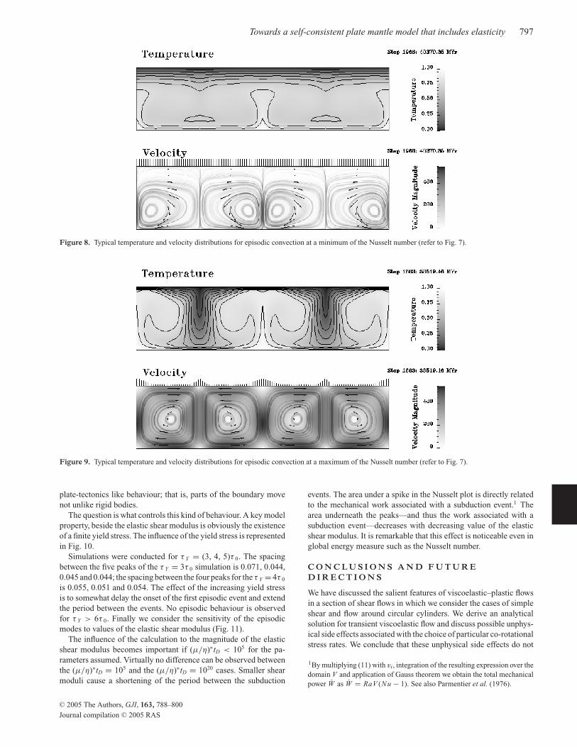
The corresponding Nusselt number vs. time plot is shown in Fig. 7.After initial, rapidly decaying primarily elastic oscillations, the sys-tem settles temporarily into stagnant lid type convection (Fig. 8).During this initial convection stresses build up until the yield stressis locally reached. The locally increased mobility is accompaniedby thermal advection, a narrow plume is forming, hot material is ad-vected underneath a narrow cold boundary layer until finally the coldlayer plunges into the model mantle along the boundary opposite tothe plume (Fig. 9).

This process repeats itself in apparently regular intervals. Thetime intervals between the first peaks of the episodic case in Fig. 7are 0.071, 0.044, 0.045, 0.044, const. spacing from then on. Alsoshown in Fig. 7 are the Nusselt numbers for mobile lid convection(obtained for τ Y = τ 0) and stagnant lid convection (τ Y ≥ 6τ 0).The isotherms and velocity arrows displayed in Figs 8 and 9 arerepresentative for the stagnant lid phases (minima of Nusselt plotsin Fig. 7) and the subduction events (maxima of Nusselt plots), forepisodic convection. Episodic behaviour based on 3-D rigid viscoplastic model is also observed by Trompert & Hansen (1998) andStein et al. (submitted 2004). Based on numerical experiments, Steinet al. have identified sub-domains in the parameter space of theirmodel of stagnant lid convection, episodic behaviour and mobile lidconvection.

The vertical lines plotted along the cold boundary of the velocityplots are the difference between the magnitude of the largest hor-izontal velocity anywhere in the domain and the magnitude of thelocal horizontal velocity on the cold boundary, divided by the largesthorizontal velocity; i.e. if the local horizontal velocity on the coldboundary happens to be the largest one, then the line has locallythe length zero. If the horizontal velocity on the cold boundary iszero (stagnant lid behaviour) the lines have uniformly the lengthone (Fig. 8). The fact that the horizontal velocity distribution on thecold boundary layer is flat on large parts of the body is indicative of

C© 2005 The Authors, GJI, 163, 788–800



Figure 8. Typical temperature and velocity distributions for episodic convection at a minimum of the Nusselt number (refer to Fig. 7).

Figure 9. Typical temperature and velocity distributions for episodic convection at a maximum of the Nusselt number (refer to Fig. 7).

plate-tectonics like behaviour; that is, parts of the boundary movenot unlike rigid bodies.

The question is what controls this kind of behaviour. A key modelproperty, beside the elastic shear modulus is obviously the existenceof a finite yield stress. The influence of the yield stress is representedin Fig. 10.

Simulations were conducted for τ Y = (3, 4, 5)τ 0. The spacingbetween the five peaks of the τ Y = 3τ 0 simulation is 0.071, 0.044,0.045 and 0.044; the spacing between the four peaks for the τ Y = 4τ 0

is 0.055, 0.051 and 0.054. The effect of the increasing yield stressis to somewhat delay the onset of the first episodic event and extendthe period between the events. No episodic behaviour is observedfor τ Y > 6τ 0. Finally we consider the sensitivity of the episodicmodes to values of the elastic shear modulus (Fig. 11).

The influence of the calculation to the magnitude of the elasticshear modulus becomes important if (µ/η)∗tD < 105 for the pa-rameters assumed. Virtually no difference can be observed betweenthe (µ/η)∗tD = 105 and the (µ/η)∗tD = 1020 cases. Smaller shearmoduli cause a shortening of the period between the subduction

events. The area under a spike in the Nusselt plot is directly relatedto the mechanical work associated with a subduction event.1 Thearea underneath the peaks—and thus the work associated with asubduction event—decreases with decreasing value of the elasticshear modulus. It is remarkable that this effect is noticeable even inglobal energy measure such as the Nusselt number.

C O N C L U S I O N S A N D F U T U R ED I R E C T I O N S

We have discussed the salient features of viscoelastic–plastic flowsin a section of shear flows in which we consider the cases of simpleshear and flow around circular cylinders. We derive an analyticalsolution for transient viscoelastic flow and discuss possible unphys-ical side effects associated with the choice of particular co-rotationalstress rates. We conclude that these unphysical side effects do not

1By multiplying (11) with vi, integration of the resulting expression over thedomain V and application of Gauss theorem we obtain the total mechanicalpower W as W = RaV (Nu − 1). See also Parmentier et al. (1976).

C© 2005 The Authors, GJI, 163, 788–800



Figure 10. The influence of the yield stress: Simulation for τ Y = (3, 4)τ 0.No episodic behaviour is observed for τ Y > 6 τ 0.

Figure 11. Influence of elastic shear modulus: (µ/η)∗tD = 0.25 104, 0.5104, 105, 1020; n = 3, npl = 15, Rac = 104, τ 0 = 0.866 102.5, τ Y = 3τ 0.

occur for stress levels possible in rocks. The latter is guaranteed ifa suitable yield criterion is included in the constitutive descriptionas proposed here and elsewhere (e.g. Moresi et al. 2002).

In the subsequent section we used the case of flow around cylin-ders to highlight parameter ranges governed by viscous, viscoplasticand viscoelasto–plastic behaviour. The local Weissenberg numberbetween the cylinders is much higher than the global Weissenbergnumber defined by the far field velocity and the cylinder radius andthe Maxwell time. This strong variation between global and localflow characteristics is not unlike the situation in mantle convectionwhere the stress in a subducting slab can be much higher than theaverage stress related to mantle size, average viscosity and averageplate speed. In the plot of the steady state values of the resultingforce on the cylinders versus the Weissenberg number we observe asharp transition between predominantly viscous to rigid plastic be-haviour with a relatively narrow interval of viscoplastic behaviourin between.

The formulation described for viscoelastic–plastic geologicalflows is based on a combined Newtonian and power-law rheology;the effect of plastic yielding is considered by an additional power-law term with a high (n ≥ 15) power-law coefficient (eq. A13).The model is valid for studying the geodynamics of mantleconvection among other problems. The non-linear equations of

motion are solved incrementally based on a consistent tangentformulation producing second-order accurate results so that iter-ations within each time step are not necessary in most cases. InMoresi & Solomatov (1998) and Tackley (1998) plastic yielding isconsidered by introducing an upper limit to the viscosity given by theratio of the yield stress and the equivalent viscous strain rate. Sincethe strain rate at the current time is unknown, an initial estimatehas to be based on the strain rate from the last time step produc-ing first-order accurate results; hence a time consuming, iterativeapproach is necessary. The iterative approach is usually more timeconsuming than the present incremental approach with occasionaliterative reduction of residuals. In the iterative approach the con-stitutive operator is more sparse than in the consistent incrementalapproach, which sometimes can be used to advantage. The con-vection problem with strongly temperature-dependent viscosity hassome unique characteristics: the strain in much of the system is verylarge, necessitating a fluid dynamics formulation, yet the relaxationtime in the cool thermal boundary layer is significant compared tothe characteristic time associated with fluid flow.

In the bulk of the fluid the relaxation time is small compared tothe time taken for convective features to evolve due to the muchlower viscosity of the warm fluid. Because elastic stresses in thestrongly convecting part of the system relax rapidly, the introductionof elasticity does not produce a qualitative change to the stagnantlid convection regime (see Solomatov 1995). In episodic and mobilelid regimes, there is a competition between the build-up of stressesin the cool lid, and the stress-limiting effect of the yield criterion.The introduction of elastic deformation does not influence this bal-ance either, although we do expect a difference in the distributionof stresses in the lid, which explains the variation in the onset ofoverturns and their increasing frequency which we observed as theelastic shear modulus was reduced. We expect also that the pres-ence of an elastic deformation mechanism allows deformation ofthe highly viscous lid with lower viscous energy-dissipation rates.This is reflected in the lower energy dissipation during episodic over-turns which we observed by integrating the system Nusselt number.In the Earth this effect may be important in subduction zones whereprediction of dissipation rates due to slab bending is unphysicallylarge. In a next step towards self-consistent plate mantle instabili-ties at the local scale of slab bending or subduction initiation areimportant. We have shown that elasticity plays a crucial role at thislocal scale.

The present power-law representation of plastic flow has the ad-vantage that strain localization due to strain softening or the fact thatpressure sensitivity is not matched by a corresponding volumetricdilatancy and is not accompanied by a change of type of the govern-ing equations (Needleman 1988). The notorious mesh sensitivityof finite element solutions (beyond the usual discretization error)does not occur in this case. We plan to expand our model to includepressure sensitivity and history dependence in the form of suitableself-consistent hardening/ softening relationships and apply the ex-tended model to more detailed studies of subduction and large-scaleshear banding.

A C K N O W L E D G M E N T S

The authors would like to acknowledge valuable comments byA/Prof L Moresi and the financial support by the AustralianComputational Earth System Simulator (ACcESS) MNRF (H M)and the Predictive Minerals Discovery CRC (PMD CRC).

C© 2005 The Authors, GJI, 163, 788–800



R E F E R E N C E S

Bercovici, D., 1993. A simple model of plate generation from mantle flow,Geophys. J. Int., 114, 635–650.

Biot, M., 1965. The Mechanics of Incremental Deformations, John Wiley,New York.

Braun, J., 1994. 3-dimensional numerical simulations of crustal-scalewrenching using a nonlinear failure criterion, Journal of Structural Geol-ogy, 16(8), 1173–1186.

Funiciello, F., Morra, G., Regenauer-Lieb, K. & Giardini, D., 2003. Dy-namics of retreating slabs: 1. Insights from two-dimensional numericalexperiments, Journal of Geophysical Research-Solid Earth, 108(B4), art.no.-2206.

Gruntfest, I.J., 1963. Thermal feedback in liquid flow; plane shear at constantstress, Transactions of the Society of Rheology, 8, 195–207.

Gurnis, M., Eloy, C. & Zhong, S.J., 1996. Free-surface formulation of mantleconvection.2. Implication for subduction-zone observables, Geophys. J.Int., 127(3), 719–727.

Harder, H., 1991. Numerical-simulation of thermal-convection withmaxwellian viscoelasticity, Journal of Non-Newtonian Fluid Mechanics,39(1), 67–88.

Hill, R., 1998. The Mathematical Theory of Plasticity, Oxford UniversityPress, Oxford.

Karato, S. & Wu, P., 1993. Rheology of the Upper Mantle: A Synthesis,Science 260, 771–778.

Kirby, S.H., 1983. Rheology of the Lithosphere, Reviews of Geophysics andSpace Physics, 21, 1458–1487.

Kolymbas, D. & Herle, I., 2003. Shear and objective stress rates in hy-poplasticity, International Journal for Numerical and Analytical Methodsin Geomechanics, 27(8), 733–744.

Leroy, Y.M. & Molinari, A., 1992. Stability of steady states in shear zones,J. Mech. Phys. Solids, 40, 181–212.

Malvern, L.E., 1969. Introduction to the Mechanics of a Continuous Medium,Prentice-Hall, New Jersey.

Melosh, H.J., 1978. Dynamic support of the outer rise, Geophys. Res. Lett.,5, 321–324.

Moresi, L. & Solomatov, V., 1998. Mantle convection with a brittle litho-sphere: thoughts on the global tectonic styles of the Earth and Venus,Geophys J. Int., 133(3), 669–682.

Moresi, L., Dufour, F. & Muhlhaus, H., 2002. Mantle convection models withviscoelastic/brittle lithosphere: numerical methodology and plate tectonicmodeling, Pageoph, 159(9), 2335–2356.

Morra, G. & Regenauer-Lieb, K., 2005. A coupled solid-fluid method formodelling subduction, Philosophical magazine, London, in press.

Muhlhaus, H.B., 1985. Surface instability of a half space with bending stiff-ness (in German), Ing. Archive, 56, 383–388.

Needleman, A., 1988. Material rate dependence and mesh sensitivity inlocalization problems. Comput. Methods Appl. Mech. Engrg., 67, 69–85.

Ogawa, M., 2003. Plate-like regime of a numerically modeled thermalconvection in a fluid with temperature-, pressure-, and stress-history-dependent viscosity, Journal of Geophysical Research-Solid Earth,108(B2), 2067–2072.

Parmentier, E.M., Turcotte, D.L. & Torrance, K.E., 1976. Studies of finiteamplitude non-Newtonian thermal convection with application to convec-tion in the Earth mantle, J. geophys. Res., 81, 1839–1846.

Phan-Thien, N., 2002. Understanding Viscoelasticity-Basics of Rheology,Springer Verlag, Berlin Heidelberg New York.

Poliakov, A., Podladchikov, Y., Dawson, E. & Talbot, C.J., 1996. Salt di-apirism with simultaneous brittle faulting and viscous flow, GeologicalSociety, 100, 291–302.

Prager, W., 1961. Introduction to Mechanics of Continua, Boston, MA: Ginn.Regenauer-Lieb, K. & Yuen, D.A., 2004. Positive feedback of interacting

ductile faults from coupling of equation of state, rheology and thermal-mechanics, Phys. Earth planet. Int., 142(1–2), 113–135.

Regenauer-Lieb, K., Yuen, D. & Branlund, J., 2001. The initation of subduc-tion: criticality by addition of water?, Science, 294, 578–580.

Schmalholz, S.M. & Podladchikov, Y., 1999. Buckling versus folding: im-portance of viscoelasticity. Geophys. Res. Lett., 26(17), 2641–2644.

Scholz, C.H., 1990. The Mechanics of Earthquakes and Faulting, CambridgeUniversity Press, Cambridge.

Solomatov, V., 1995. Scaling of temperature-dependent and stress-dependentviscosity convection. Physics of Fluids, 7(2), 266–274.

Stein, C.A., Schmalzl, J. & Hansen, U., 2004. The effect of rheological pa-rameters on plate behaviour in a self-consitent model of mantle convection,Phys. Earth planet. Int., 142(3–4), 225–255.

Tackley, P., 1998. Self-consistent generation of tectonic plates in three-dimensional mantle convection, Earth planet. Sci. Lett., 157, 9–22.

Tackley, P., 2000a. Self-consistent generation of tectonic plates in time-dependent, three-dimensional mantle convection simulations, 1. Pseudo-plastic yielding, G3, 01(23), 1525.

Tackley, P., 2000b. Self-consistent generation of tectonic plates in time-dependent, three-dimensional mantle convection simulations. 2. Strainweakening and asthenosphere, G3, 01(25), 2027.

Trompert, R. & Hansen, U., 1998. Mantle convection simulationswith rheologies that generate plate-like behavior, Nature, 395, 686–689.

Turcotte, D.L. & Schubert, G., 2002. Geodynamics, 2nd edn, CambridgeUniversity Press, Cambridge.

Zienkiewicz, O.C. & Taylor, R.L., 2000. The Finite Element Method, 5thedn, Butterworth/Heinemann, Oxford, ISBN 0 7506 5050 8, 3.

A P P E N D I X

A1 Simple shear

The following derivations are based on the assumption of the Jau-mann rate in the constitutive relationships (2). It should be men-tioned that for simple shear the Jaumann rate based model and theOldroyd based model are identical. For isothermal, plane simpleshear parallel to x1, the equilibrium conditions read:

σ12,2 = 0,

σ22,2 = 0. (A1)

From the general definition of the Jaumann stress rate

σ Ji j = σi j − Wikσk j + σik Wkj , (A2)

we obtain for simple shear:

σ ′J22 = −σ ′J

11 = σ ′22 − 1

2(v2,1 − v1,2)σ12 − σ21

1

2(v2,1 − v1,2)

= σ ′22 + v1,2σ12,

σ J12 = σ12 − 1

2v1,2σ

′22 + σ ′

11

1

2v1,2

= σ12 − v1,2σ′22.

(A3)

Insertion into the constitutive relationship (2) yields:

λσ12 − λγ σ ′22 + σ12 = ηγ ,

λσ ′22 + λγ σ12 + σ ′

22 = 0, (A4)

where

γ = v1,2, λ = η

µand η =

(1

ηN+ 1

ηN (τ/τ0)1−n

)−1

. (A5)

In steady state the stress rate in A4 disappears; elimination of σ 22

yields eq. (22) in the simple shear section.

A2 Tangent operator

Incremental expansion of the constitutive relation

Di j = 1

2µσ ′J

i j + 1

2ησ ′

i j + γ pσ ′

i j

2τ, (A6)

C© 2005 The Authors, GJI, 163, 788–800



with a power-law evolution equation for γ p

γ p = τY

ηY

(τ

τY

)n pl

, (A7)

and η is defined by eq. (7), yields:

Di j − δt

2ηeff(Wikσk j − σik Wkj ) − 1

2µσ ′

i j,kvk = 1

2µeffδtδσ ′J

i j

+(

1

hvis+ 1

hY

)︸︷︷︸

1/h

σ ′i j

2τ

σ ′kl

2τδσ ′J

kl + 1

2ηeffσ ′

i j + 1

2ηeffσ ′

i j

(δT

hT+ δp

h p

),

(A8)

where

σ ′i j = σ ′

i j,t + σ ′i j,kvk, (A9)

δσ Ji j = (σi j,t − Wikσk j + σik Wkj )δt, δT = T,tδt, δp = p,tδt

(A10)

hvis = 1

(n − 1)ηN

(τ

τ0

)1−n

, and hY = 1

(n pl − 1)ηY

(τ

τY

)1−n pl

(A11)

hT = T 2

ATM, h p = − T

A ∂TM∂p

, (A12)

where ηN is defined by (6) and

ηeff = 1

ηN+ 1

ηN

(τ

τ0

)1−n + 1

ηY

(τ

τY

)1−n pl

−1

,

µeff =(

1

µ+ δt

ηeff

)−1

. (A13)

Inversion of A8 yields:

δσ ′Ji j =

(µeffδt(δikδ jl + δ jkδil ) − (µeffδt)2

h + µeffδt

σ ′i j

τ

σ ′kl

τ

)

×(

Dkl − σ ′kl,mvm

2µ

)− µeffδt

ηeff

(1 − µeffδt

h + µeffδt

)

×(

1 + δT

hT+ δp

h p

)σ ′

i j − µeffδt2

ηeff(Wikσk j − σik Wkj ),

(A14)

where

h = hvishY

hvis + hY. (A15)

The function hp in eqs (A8) and (A14) considers the pressure depen-dence of TM . The slope of the TM –p curve is usually assumed as con-stant; a typical order of magnitude value for the slope is 10−7 K Pa −1.For n = 1 and µ → ∞ we obtain Newtonian flow with the viscosity1/2ηN .

In many practical applications the velocity problem, the pres-sure/incompressibility problem and the heat equation are solvedsequentially. In this case the terms associated with δT and δ p in eq.(A14) are not needed. In linear instability analyses however the fullincremental form (A14) is required.

In the viscous limit, µ → ∞, (A14) reduces to:

δσ ′i j =

(ηeff(δikδ jl + δ jkδil ) − η2

eff

h + ηeff

σ ′i j

τ

σ ′kl

τ

)Dkl

−(

1 − ηeff

h + ηeff

) (1 + δT

hT+ δp

h p

)σ ′

i j .(A16)

In steady states, the stress, temperature and pressure incrementsvanish so that the remaining terms in (A16) have to cancel. Thelatter is indeed the case as can be shown by insertion of Dij =1/2ηeff σ ′

i j .The limit ηN → ∞ does not yield a simpler expression for the

incremental relationship A14 since the effective moduli still dependon the viscosity ηY (τ Y /τ )n pl−1. In the rate-independent limit, whichis obtained for ηN → ∞, npl → ∞ and δt → 0, the expression A14reduces to

∂σ ′i j/∂t =

(µ(δikδ jl + δ jkδil ) − µ

σ ′i j

τ

σ ′kl

τ

) (Dkl − 1

2µσ ′

i j,kvk

)

+ (Wikσk j − σik Wkj ). (A17)

In the above derivations it was always assumed that the yield stressis constant. A large deformation model with power-law plasticitywith state variable dependence of the yield stress will be presentedin a forthcoming paper.

C© 2005 The Authors, GJI, 163, 788–800


Documents

Towardsaself-consistent plate mantle model that … · Towardsaself-consistent plate mantle model that ... Maxwell model that explains many of the difﬁculties he has strug-