Embed Size (px)
Citation preview
Centre of Mathematical Modelling and Flow Analysis
Department of Computing and Mathematics
Manchester Metropolitan University
Towards the Numerical Simulation of Ship Generated Waves Using aCartesian Cut Cell Based Free Surface Solver
Jose Antonio Armesto Alvarez
December 2008
A Thesis Submitted in Partial Fullfilment
of the Requirements for the Degree of
Doctor of Philosophy.

Towards the Numerical Simulation of Ship Generated Waves Using aCartesian Cut Cell Based Free Surface Solver
Jose Antonio Armesto Alvarez
Centre for Mathematical Modelling and Flow Analysis
Manchester Metropolitan University
John Dalton Building
Chester Street
Manchester M1 5GD, UK.
December 2008

Contents
List of Acronyms iii
List of Figures v
List of Tables xi
Abstract xiii
Declaration xv
Acknowledgements xvii
Agradecimientos xix
Chapter 1. Introduction 11. Motivation 12. Grid Methods 33. Alternative Equations that were Dismissed 54. Navier-Stokes Equations 95. Alternative Solution Methods 146. Outline of the Thesis 23
Chapter 2. Cartesian Cut Cell Method 251. Introduction 252. Cutting the Grid Around the Solid 273. Cells Merging 304. Intersecting Solid and Free Surface 335. Cartesian Cut Cell Routines 36
Chapter 3. Numerical Method 431. Introduction 432. Artificial Compressibility Method 443. Godunov’s Method 464. Flux Calculation 485. The Riemann Problem 536. Merged Cells Contributions 587. Boundary Conditions 598. Linearization 629. Linear System 6510. Solution Scheme 67
Chapter 4. Free Surface 691. Introduction 692. Interface Capturing Methods 703. Interface Tracking Methods 74
i
ii CONTENTS
4. Pressure on Free Surface Flows 785. Boundary Conditions at the Free Surface 786. Solid and Free Surface Cutting Each Other 80
Chapter 5. Numerical Experiments: No Free Surface 831. Lid-driven Couette Flow 832. Lid-Driven Cavity Flow 843. Current Flow in a Pipe 924. Current Flow in a Pipe with an Obstacle. 97
Chapter 6. Numerical Experiments: Free Surface 1011. Small Amplitude Sloshing Tank 1012. Mass-Wave Maker 1153. Semi Dam Break 1164. Current Flow Passing Over a Bump 1215. Current Flow Passing a Cylindrical Body in the Flow 1306. Current Flow Passing a Cylinder at the Free Surface 139
Chapter 7. Conclusions and Future Work 1431. Conclusions 1432. Future Work 144
List of References 147
Appendix A. Publications 157
List of Acronyms
ACM Artificial Compressibility MethodALE Arbitrary Lagrangian-Eulerian MethodsALU Approximate Lower Upper (LU) FactorizationCCCM Cartesian Cut Cell MethodCCCR Cartesian Cut Cell RoutinesCFD Computational Fluid DynamicsCFPOB Current Flow Passing Over a BumpCFPCFS Current Flow Passing a Cylinder at the Free SurfaceCFPCBF Current Flow Passing a Cylindrical Body in the FlowCMMFA Centre of Mathematical Modelling and Flow AnalysisEE Euler EquationFDM Finite Difference MethodsFEM Finite Element MethodsFVM Finite Volume MethodsGNE Green-Naghdi equationsHLL Harten, Lax and Van Leer (Riemann solver)LBM Lattice Boltzmann MethodLBG-BGK Lattice Boltzmann Method Bhatnagar-Gross-KrookLGA Lattice Gas AutomataLHS Left Hand SideLSM Level Set MethodMAC Marker and CellMMU Manchester Metropolitan UniversityNSE Navier-Stokes EquationsODE Ordinary Differential EquationPDE Partial Differential EquationRANS Reynolds-Averaged Navier-Stokes EquationsRHS Right Hand SideR-K Runge-Kutta MethodsRP Riemann ProblemRS Riemann SolverSEM Spectral Element MethodsSPH Smoothed Particle HydrodynamicsSWE Shallow Water EquationsVoF Volume of Fluids
iii

List of Figures
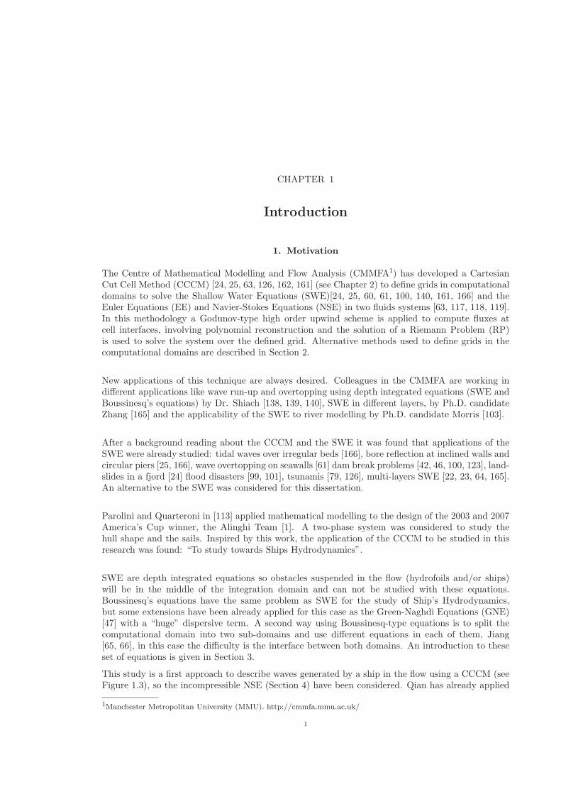
1.1 Laboratory experiments at the Ship Model Tank from the Ship Technology Department ofMARINTEK, SINTEF [8]. 2
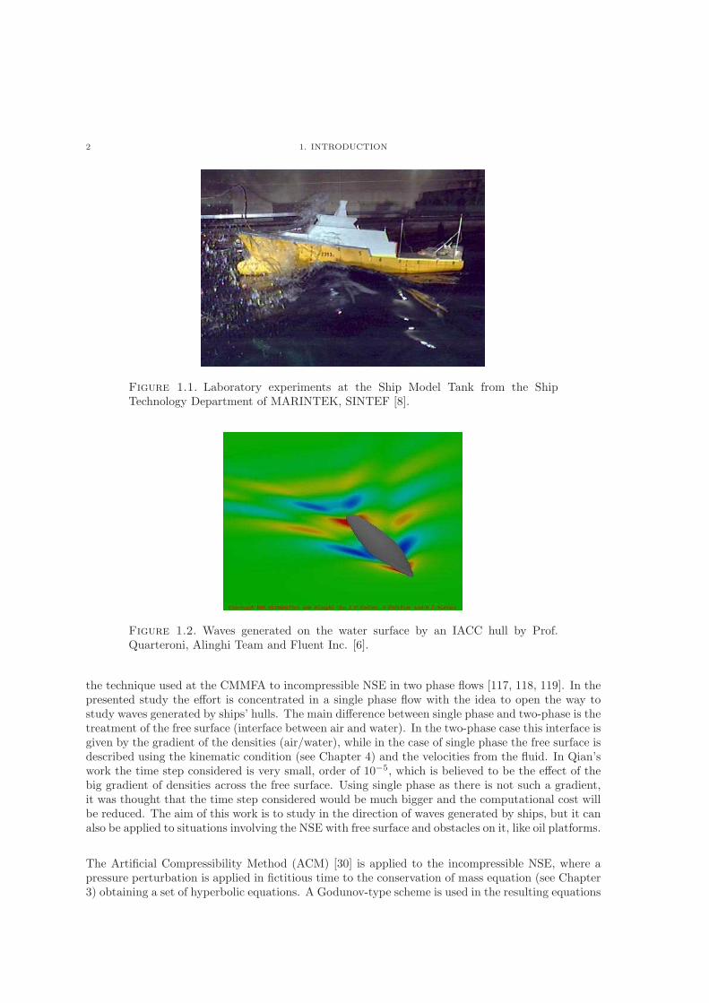
1.2 Waves generated on the water surface by an IACC hull by Prof. Quarteroni, Alinghi Teamand Fluent Inc. [6]. 2
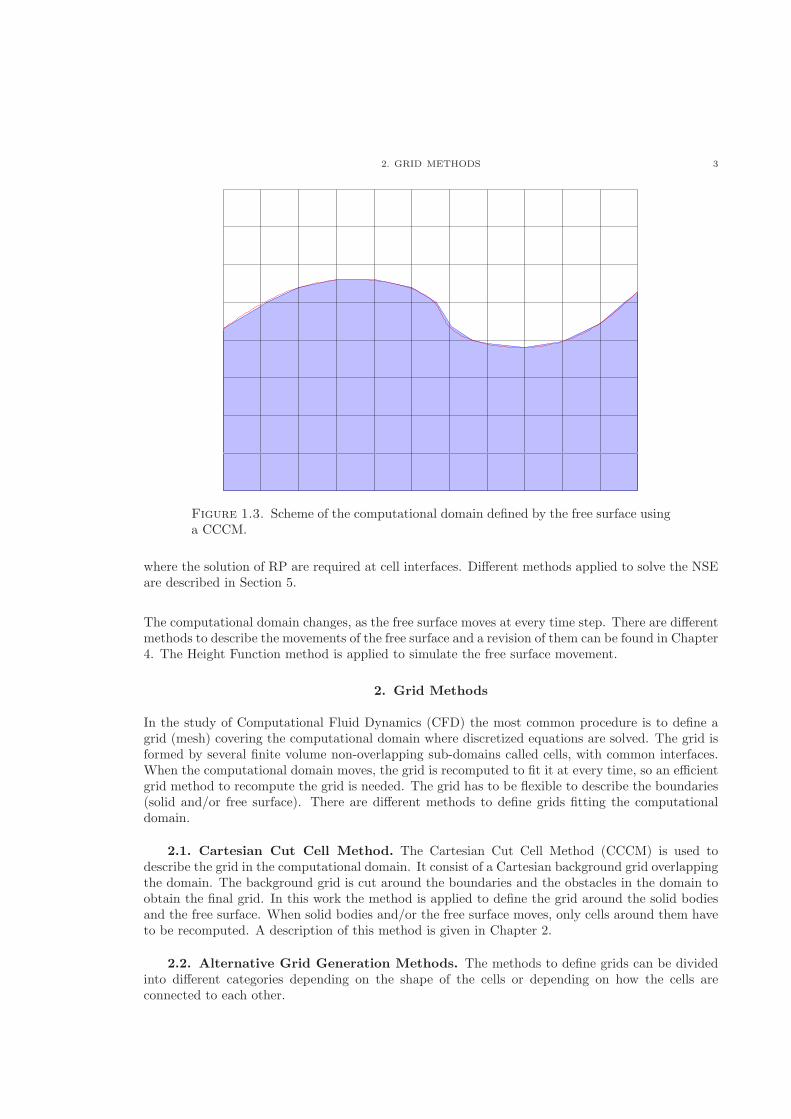
1.3 Scheme of the computational domain defined by the free surface using a CCCM. 3
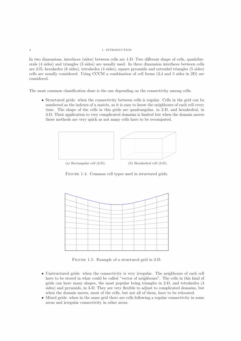
1.4 Common cell types used in structured grids. 4
1.5 Example of a structured grid in 2-D. 4
1.6 Common cell types used in unstructured grids. 5
1.7 Example of an unstructured grid in 2-D. 5
1.8 Example of a mixed grid in 2-D. 5
1.9 Notation used in the SWE. 6
1.10Situations that can and can not be dealt with using SWE. 7
1.11Scheme of the domains proposed by Jiang [65, 66]. 8
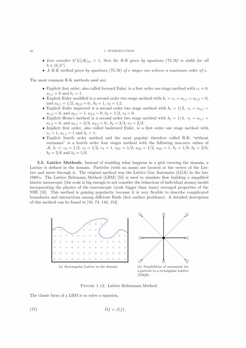
1.12Lattice Boltzmann Method. 20
1.13Scheme of the particles in the domain. 21
2.1 Flags: (a) Flow cell, (b) Cut cell and (c) Solid cell. 25
2.2 (a) Simple cut given by the CCCM. (b) Corner cut which can not be described by theCCCM. 26
2.3 Intermediate steps of a flow cell becoming solid cell due the movement of the solid body. 26
2.4 The computational domain is the FLOW part (water) while the Air part is of no interestin this study and is all the part above the free surface. Approximation of the cuts avoidingcorners in cut cells is shown as well as merged cells. 27
2.5 Notation used with respect to cell (i, j). 28
2.6 Computing the intersection points with the grid. a = (xa, yj), b = (xi+1, yb) andc = (xc, yj+1) 29
2.7 Cell types for Slope(i, j) = 1, where coloured part is solid. 29
2.8 Cell types for Slope(i, j) = 2, where coloured part is solid. 29
2.9 Cell types for Slope(i, j) = 3, where coloured part is solid. 30
2.10Cell types for Slope(i, j) = 4, where coloured part is solid. 30
2.11Area of cut cell A is smaller than Amin and is merged with surrounding cell B formingsuper-cell C. 31
2.12Merge small flow cells. 31
2.13Super-cell containing cells A, B, C, D, E and F when merging at the free surface. 32
2.14Cut between the solid (red) and the free surface (blue) in one cell. 33
v
vi LIST OF FIGURES
2.15Cut between the solid (red) and the free surface (blue) in one cell. Sfs and Efs are thestart and end points from the free surface, Ss and Es are the start and end points from thesolid obstacle. Point C is the intersection point between both cuts. 34
2.16Cell of type 1 for Slopes(i, j) = 1. The red colored part is the solid and the blue is the freesurface (air). 36
2.17Cell of type 2 for Slopes(i, j) = 1. The red colored part is the solid and the blue is the freesurface (air). 36
2.18Cell of type 3 for Slopes(i, j) = 1. The red colored part is the solid and the blue is the freesurface (air). 37
2.19Cell of type 4 for Slopes(i, j) = 1. The red colored part is the solid and the blue is the freesurface (air). 37
2.20Position of the solid bodies given in the example. 38
2.21Grid resultant of applying the CCCR to the geometry given. Merged cells A, B, C, D andE. 40
3.1 Reconstructed values (i+ 1, j) and UL(i+1/2,j) at each side of cell interface (i+ 1/2, j). 50
3.2 Locate point R. 51
3.3 Gradients for the solid cut cell. 52
3.4 (a) Rarefaction wave, (b) Shock wave and (c) Contact discontinuity. 55
3.5 Division of the space produced by the three waves (�1, �2 and �3). 55
3.6 Boundary cell (i, j) and its ghost cell (ig, jg). 60
3.7 Mesh � with ghost cells at boundaries x = a, {(0, j) : j = 1, 2, . . . ,M} and x = b,{(M + 1, j) : j = 1, 2, . . . ,M}. 60
4.1 Distribution of markers in the MAC method. 70
4.2 Values of function � in the VoF method. 73
4.3 Reconstruction of the free surface using the VoF method. 73
4.4 Movement of the control points from the free surface at time t = tn, to the free surface attime t = tn+1 (dotted line). 74
4.5 Situations where function ℎ would be multi-valued. 75
4.6 Unitary n normal and t tangential vectors and curvature K of the free surface. 79
4.7 Velocities (V = Vf − Vg) at the free surface and cell interfaces. 80
4.8 Cut between the solid (red) and the free surface (blue) in one cell. 81
5.1 Scheme of the lid driven Couette problem 83
5.2 Scheme of the lid driven cavity problem 85
5.3 Results of the lid driven cavity flow using Roe’s RS, Re = 100, N =M = 50, � = 0.01 andΔ� = 106. 85
5.4 Logarithm of ∣∣Un+1 −Un∣∣2 for both RS. The following values have been considered, for agrid size 50× 50, � = 0.01, Re = 100, Δ� = 100000 and Δt = 1 with Tend = 100. 86
5.5 Horizontal velocities along x = 0.5 with HLL (top) and Roe’s (bottom) RS. 88
5.6 Comparison of the horizontal velocities along x = 0.5 using both RS andRe = 50, 100, 400, 1000, 2000, 5000. 89
5.7 Vertical velocities along y = 0.5 with HLL (top) and Roe’s (bottom) RS. 90
LIST OF FIGURES vii
5.8 Comparison of the vertical velocities along y = 0.5 using both RS andRe = 50, 100, 400, 1000, 2000, 5000. 91
5.9 Layer flow in a domain Ω = [0, 10]× [0, 1]. 92
5.10Velocity profile at final time (Tend = 100) using the Roe’s RS with V = 1.5, Δt = 0.5,Re = 50 and � = 2.5. 92
5.11Horizontal velocities at the end of the pipe (x = 10) using Re = 1000. 94
5.12Logarithm of ∣∣Un+1 −Un∣∣2 during the computation using Re = 1000. 94
5.13Horizontal velocities at the end of the pipe (x = 10) using Re = 1000 and � = 10. 95
5.14Logarithm of ∣∣Un+1 −Un∣∣2 during the computation using Re = 1000 and � = 10. 95
5.15Horizontal velocities at the end of the pipe (x = 10) using Re = 500. 96
5.16Logarithm of ∣∣Un+1 −Un∣∣2 during the computation using Re = 1000. 96
5.17Current flow in a pipe Ω = [0, 40] × [0, 20], with cylindrical obstacle of centre C = (10, 10)
and radius r = 1, and inflow velocity Vin = (1, 0)T . 97
5.18Drag cD and lift cL coefficients computed using the Roe’s RS, N = 100, M = 50,Δt = 1/100 and � = 1.5. 98
5.19Velocity profile using both RS at final time t = 300, N = 100, M = 50, Δt = 1/100 and� = 1.5. 99
5.20Streamlines produced using HLL and Roe’s RS at t = 272 and t = 276. N = 100, M = 50,Δt = 1/100 and � = 1.5. 100
6.1 Initial position of the free surface. 102
6.2 Free surface elevation of the first point for different � values (500 − 50000), usingN =M = 120 and Δt = 1/500. 103
6.3 Free surface elevation of the first point for different � values (0.01 − 500000), usingN =M = 60 and Δt = 1/20. 104
6.4 Free surface elevation of the first point for different time steps (Δ = 1/20, 1/100, 1/500),using different grid sizes (N, M) and � = 1.5. 105
6.5 Free surface elevation of the first point for different time steps (Δ = 1/20, 1/100, 1/500),using different grid sizes (N, M) and � = 500. 106
6.6 Free surface elevation of the first point for different time steps (Δ = 1/20, 1/100, 1/500),using different grid sizes (N, M) and � = 50000. 107
6.7 Free surface elevation of the first point for different time steps (Δ = 1/20, 1/100, 1/500),using different grid sizes (N, M) and � = 500000. 108
6.8 Free surface elevation of the first point for different spatial configurations,N =M = (30, 60, 120), using different time intervals Δt and � = 1.5. 109
6.9 Initial position of the free surface. 110
6.10Position of the free surface for different values of the Reynolds numbers(Re = 2, 20, 200, 2000, 20000) using M × N = 120 × 120, Δt = 1/60 and� = 1.5. 111
6.11Position of the free surface using diferent Re = 100, N = M = 120, � = 1.5 and differentvalues of the time step. 112
6.12Position of the free surface using diferent Re = 100, N = M = 120, time step Δt = 1/120and different values of �. 112
6.13Free surface elevation of the middle point for � = 0.5, using different grid sizesN =M = (30, 60, 120) and different time steps Δt = (1/10, 1/60, 1/100, 1/120). 113
viii LIST OF FIGURES
6.14Free surface elevation of the middle point for � = 1.5, using different grid sizesN =M = (30, 60, 120) and different time steps Δt = (1/60, 1/100, 1/120). 114
6.15Scheme of the mass-wave maker problem. The red square represents the area of the masssource. 115
6.16Free surface elevation at time T = 4 s. and T = 8 s. using N = 201 and M = 50,Δt = 1/500 and different values of � = 500, 2000, 200000. 116
6.17Scheme of the “full” dam break problem. 117
6.18Scheme of the semi dam break problem. 117
6.19Free surface elevation at different times for N = 200, M = 40, � = 500 and different valuesof the time step Δt = 1/200 (891.35 CPU sec), 1/500 (1881.17 CPU sec), 1/1000 (3085.13CPU sec). 118
6.20Free surface elevation at different times for N = 200, M = 40, Δt = 1/500 and differentvalues of � = 500 (1881.17 CPU sec), 2000 (1609.19 CPU sec), 5000 (2027.31 CPU sec). 119
6.21Free surface elevation at different times for N = 200, M = 40, Δt = 1/1000 and differentvalues of � = 500 (3085.13 CPU sec), 5000 (3167.69 CPU sec), 50000 (5602.10 CPU sec). 120
6.22Scheme of the CFPOB problem. 121
6.23Velocity profile of the CFPOB problem after 20 seconds using � = 5, Δt = 1/50. 121
6.24Free surface elevation at different times for N = 300, M = 30, Δt = 1/20 and differentvalues of � = 1, 5, 50, 500. 123
6.25Free surface elevation at different times for N = 300, M = 30, Δt = 1/100 and differentvalues of � = 1, 5, 50. 124
6.26Free surface elevation at different times for N = 300, M = 30, different time stepsΔt = 1/20, 1/50, 1/100, 1/400 and � = 5. 125
6.27Velocity profile of the CFPOB problem after 20 seconds using Reynolds number Re = 200,� = 0.6, Δt = 1/100. 126
6.28Free surface elevation at different times for N = 300, M = 30, different time stepsΔt = 1/66, 1/100, 1/200 and � = 0.5. tol = 10−5 127
6.29Free surface elevation at different times for N = 300, M = 30, different time stepsΔt = 1/66, 1/100, 1/200 and � = 0.6. tol = 10−5 128
6.30Free surface elevation at different times for N = 300, M = 30, time step Δt = 1/100 anddifferent values of �(= 0.1, 0.5, 0.6, 1, 1.5). tol = 10−5 129
6.31Scheme of the CFPCBF problem. 130
6.32Velocity profile of the CFPCBF after 20 seconds using � = 1, Δt = 1/50. 130
6.33Free surface elevation at different times for N = 300, M = 30, time steps Δt = 1/20 anddifferent values of �(= 5, 50, 500). 132
6.34Free surface elevation at different times for N = 300, M = 30, time steps Δt = 1/100 anddifferent values of �(= 1, 5, 50, 500). 133
6.35Free surface elevation at different times for N = 300, M = 30, different time stepsΔt = 1/20, 1/50, 1/100 and � = 5. tol = 10−5 134
6.36Velocity profile of the CFPCBF problem after 20 seconds using Reynolds number Re = 200,� = 1, Δt = 1/200. 135
6.37Free surface elevation at different times for N = 300, M = 30, different time stepsΔt = 1/50, 1/100, 1/200 and � = 0.5. tol = 10−5 136
6.38Free surface elevation at different times for N = 300, M = 30, different time stepsΔt = 1/50, 1/100, 1/200 and � = 0.6. tol = 10−5 137
LIST OF FIGURES ix
6.39Free surface elevation at different times for N = 300, M = 30, different values of�(= 0.1, 0.5, 0.6, 1, 1.5) and time step Δt = 1/100. tol = 10−5 138
6.40Scheme of the CFPCFS problem. 139
6.41Free surface elevation at different different times for N = 300, M = 30, different values of�(= 500, 1000, 5000) and time step Δt = 1/100. tol = 4 ⋅ 10−4. 140
6.42Velocity profile of the current flow passing a cylinder at the free surface. Velocity at onecell is so hight it does not allow to see more than that cell. Free surface is represented by ablack line. 141
6.43Velocity profile of the current flow passing a cylinder at the free surface, where velocityplotted between 0 and 2. 141

List of Tables
5.1 Errors obtained using both RS once the steady state is reached. Δx = Δy = 0.1, Δt = 0.1,� = 1, � = 0.001. 84
5.2 Cell center of the cell containing the primary vortex in a grid 50× 50 for a range of differentcompressibility coefficients �. 86
5.3 Cell centre of the cell containing the primary vortex in different grid sizes for � = 0.01. Thefollowing values have been considered, � = 0.01, Re = 100, Δ� = 100000 and Δt = 1 withTend = 100. 86
5.4 Running times for the versions with both RS. The following values have been considered,grid size 50 × 50, so Δx = Δy = 0.02, Re = 100, Δ� = 100000 and Δt = 0.1 withTend = 100. tol = 10−5. 87
5.5 Running times for the versions with both RS. The same values have been considered butΔt = 1 87
5.6 Errors at the final time for a range of Reynolds numbers. Grid size 150 × 150 but forRe = 7500 the grid size is 250× 250. 88
5.7 Case 1, computational times in seconds. ∗ denotes values obtained using formula (114). 93
5.8 Case 2, computational times in seconds. ∗ values obtained using formula (114). 94
5.9 Case 3, computational times in seconds. ∗ values obtained using formula (114). 95
6.1 Computational times in CPU seconds using different values of � and Δt in a gridN =M = 30. Divergent results are illustrated by ⋅, tol = 10−6 102
6.2 Computational times in CPU seconds using different values of � and Δt in a gridN =M = 60. Divergent results are illustrated by ⋅, tol = 10−6 102
6.3 Computational times in CPU seconds using different values of � and Δt in a gridN =M = 120. Divergent results are illustrated by ⋅, tol = 10−6 103
6.4 Computational times in CPU seconds using different values of � and Δt in a gridN =M = 30 for Re = 100. Divergent results are illustrated by ⋅, tol = 10−6. 110
6.5 Computational times in CPU seconds using different values of � and Δt in a gridN =M = 60 for Re = 100. Divergent results are illustrated by ⋅, tol = 10−6. 111
6.6 Computational times in CPU seconds using different values of � and Δt in a gridN =M = 120 for Re = 100. Divergent results are illustrated by ⋅, tol = 10−6. 111
6.7 Computational times in CPU seconds using a grid N ×M = 300× 30, different values of �and Δt. Divergent results are illustrated by ⋅, tol = 10−5. 122
6.8 Computational times in CPU seconds using Re = 200, a grid N ×M = 300× 30, differentvalues of � and Δt. Divergent results are illustrated by ⋅, tol = 10−5. 126
6.9 Computational times in CPU seconds using a grid N ×M = 300× 30, different values of �and Δt. Divergent results are illustrated by ⋅, tol = 10−5. 131
xi
xii LIST OF TABLES
6.10Computational times in CPU seconds using Re = 200, a grid N ×M = 300× 30, differentvalues of � and Δt. Divergent results are illustrated by ⋅, tol = 10−5. 135
Abstract
The Cartesian Cut Cell method has been applied to different flow configurations by researchersat the Centre of Mathematical Modelling and Flow Analysis. This method has been implementerto define flow domains around obstacles using a Godunov-type high order upwind scheme to solveShallow Water Equations and Navier-Stokes (Euler) equations in two phase flows.
A new idea to study Navier-Stoke (Euler) equations in just one phase flows where the domain isaccurate described using the Cartesian Cut Cell Method around the moving free surface is presented.The solution technique involves three stages for every time step: the definition of the domain, thesolution of the flow equations and the movement of the free surface. The Cartesian Cut Cell Methodonly requires to recompute cells affected by the movement of the free surface obtaining providingquickly the new domain. The flow equations are solved using the Artificial Compressibility Methodand a Godunov-type high order upwind scheme involving the solution of Riemann problems. TheHeigh Function method is applied to study the evolution on time of the free surface. This methodinvolves the solution of the kinematic equations, where a fourth order Runge-Kutta method is em-ployed. Boundary conditions at the free surface are discussed.
The technique proposed is very quick and allows the use of big time steps. In comparison with thetwo phase version, the proposed techniques used one thousand times bigger time steps and requirearound 25 times less computational effort. On the other hand, the results shows dependency on theartificial compressibility parameter introduced as part of the solution of the flow equations. Exten-sions to the presented study are proposed including the use of different flow solvers.
An algorithm to solve free surface flows in a single phase system is presented. The Cartesian CutCell Method is used to define the grid in a domain involving free surface and/or the presence of anobstacle. The algorithm approximate the solutions of the incompressible Navier-Stokes equationsbased on the Artificial Compressibility Method and uses the cell-centred finite volume approach. AGodunov-type high order upwind scheme is applied to compute fluxes at cell interfaces, involvingpolynomial reconstruction and the solution of a Riemann problem. The HLL Riemann solver andRoe’s Riemann solver are implemented as part of the Godunov-type upwind scheme. An implicitscheme is used for the time discretization in problems without free surface while an explicit forthorder Runge-Kutta method is used in free surface problems. An introduction to problem where thefree surface and the obstacle cut each other is presented.
xiii

Declaration
No portion of the work referred to in this Thesis has been submitted in support of an applicationfor another degree or qualification at this or any other university or other institution of learning.
Apart from those parts of this Thesis which contain citations to the work of others and apart fromthe assistance mentioned in the acknowledgements, this Thesis is my own work.
Jose Antonio Armesto Alvarez
xv

Acknowledgements
I would like to thank my supervisors Mr. Clive Mingham, Dr. Ling Qian and Prof. Derek Causon fortheir support and guidance throughout my studies. I would also like to thank the Manchester Met-ropolitan University for the economical support provided for this Thesis. I would also like to thankmy former supervisor Dr. David Ingram and my fellow colleagues at the Centre of MathematicalMethods and Flow Analysis and specially to Mr. Andrew Morris for all the informal discussions wehad about the Cartesian Cut Cell routines and Dr. Wei Bai for his very useful criticism of my work.My gratitude to my office colleagues Dr. Ben Cawley, Mr. Yong Zang, Mr. Stavros Tentonidis, Ms.Fieke Geurtz and Mr. Kevin Bennet for the enjoyable work atmosphere and the lunches at Tai Wu.
My gratitude to Mr. Adrian Sarasquete for his help to open my eyes to new methods at the con-ferences “MARINE CFD 2005” and “Marine 2007, II International Conference on ComputationalMethods in Marine Engineering” and Dr. Antonio Souto Iglesias and Prof. Raul Medina Santamarıafor giving me the opportunity to present my work at the Universidad Politecnica de Madrid in April2008 and at the Instituto de Hidraulica Ambiental “IH Cantabria”, Universidad de Cantabria inOctober 2008 respectively. Many thanks to Mr. Koushan from SINTEF for permitting me the useof their picture in Figure 1.1 and Prof. Quarteroni, Dr. Parolini, Ms. Eugenia Manzanas from theAlinghi Team and Fluent Inc. for their picture used in Figure 1.2.
Finally I would like to thanks my girlfriend Marıa for her support, comprehension and love andmy family for their support during the last years. During my time in Manchester I made manyfriends and team-mates from the Manchester Handball Club, Jorge, Marıa, Jean Charles, Rakel,Karim, James, Minas, Lukasz..., and friends and enemies from the Manchester University HandballClub, Asier, Krasi, Marta, Luis, Ralf, Chris, Dominik, Damien,.... To all of them and my friends inValladolid, Adolfo, Raul, Pilar, David, Jose Luis... and Kaiserslautern, Lolo, Fernando, Jonathan,Panos, Julio, Diego,... I would like to thank.
xvii

Agradecimientos
Me gustarıa agradecerles el apoyo y su dedicacion a mis directores de tesis, D. Clive Mingham, Dr.Ling Qian y Prof. Derek Causon. Mi agradecimiento a la Manchester Metropolitan University elapoyo economico prestado para la realizacion de esta Tesis. Me gustarıa agradecer tambien a miex-director Dr. David Ingram y a mis companeros del Centre of Mathematical Methods and FlowAnalysis y especialmente a D. Andrew Morris por las discusiones informales mantenidas sobre lasrutinas del Cartesian Cut Cell y al Dr. Wei Bai por sus extremadamente utiles criticas a mi trabajo.Mi agradecimiento a mis companheros de despacho Dr. Ben Cawley, D. Yong Zang, D. Stavros Ten-tonidis, Da. Fieke Geurtz y D. Kevin Bennet por el magnifico ambiente de trabajo y los almuerzosen Tai Wu.
Mi agradecimiento a D. Adrian Sarasquete por su ayuda en la participacion de conferencias como“MARINE CFD 2005” and “Marine 2007, II International Conference on Computational Methods inMarine Engineering” y al Dr. Antonio Souto Iglesias y al Prof. Raul Medina Santamarıa por darmela oportunidad de exponer mi trabajo en la Universidad Politecnica de Madrid en Abril de 2008 yel el Instituto de Hidraulica Ambiental “IH Cantabria” de la Universidad de Cantabria en Octubrede 2008 respectivamente. Muchas gracias al Sr. Koushan de SINTEF por permitirme utilizar suimagen en Figure 1.1 y Prof. Quarteroni, Dr. Parolini, Da. Eugenia Manzanas del Alinghi Team yFluent Inc. por su imagen utilizada en Figure 1.2.
Finalmente me gustaria agradecer a mi novia Marıa su paciencia, apoyo y comprension, y a mi familiasu apoyo durante los ultimos anos. Durante mi estancia en Manchester he hecho muchos amigos demi equipo, el Manchester Handball Club Jorge, Marıa, Jean Charles, Rakel, Karim, James, Minas,Lukasz..., del equipo rival, el Manchester University Handball Club Asier, Krasi, Marta, Luis, Ralf,Chris, Dominik, Damien,.... A todos ellos y a mis amigos de Valladolid, Adolfo, Raul, Pilar, David,Jose Luis,... y Kaiserslautern, Lolo, Fernando, Jonathan, Panos, Julio, Diego,... muchas gracias.
xix

CHAPTER 1
Introduction
1. Motivation
The Centre of Mathematical Modelling and Flow Analysis (CMMFA1) has developed a CartesianCut Cell Method (CCCM) [24, 25, 63, 126, 162, 161] (see Chapter 2) to define grids in computationaldomains to solve the Shallow Water Equations (SWE)[24, 25, 60, 61, 100, 140, 161, 166] and theEuler Equations (EE) and Navier-Stokes Equations (NSE) in two fluids systems [63, 117, 118, 119].In this methodology a Godunov-type high order upwind scheme is applied to compute fluxes atcell interfaces, involving polynomial reconstruction and the solution of a Riemann Problem (RP)is used to solve the system over the defined grid. Alternative methods used to define grids in thecomputational domains are described in Section 2.
New applications of this technique are always desired. Colleagues in the CMMFA are working indifferent applications like wave run-up and overtopping using depth integrated equations (SWE andBoussinesq’s equations) by Dr. Shiach [138, 139, 140], SWE in different layers, by Ph.D. candidateZhang [165] and the applicability of the SWE to river modelling by Ph.D. candidate Morris [103].
After a background reading about the CCCM and the SWE it was found that applications of theSWE were already studied: tidal waves over irregular beds [166], bore reflection at inclined walls andcircular piers [25, 166], wave overtopping on seawalls [61] dam break problems [42, 46, 100, 123], land-slides in a fjord [24] flood disasters [99, 101], tsunamis [79, 126], multi-layers SWE [22, 23, 64, 165].An alternative to the SWE was considered for this dissertation.
Parolini and Quarteroni in [113] applied mathematical modelling to the design of the 2003 and 2007America’s Cup winner, the Alinghi Team [1]. A two-phase system was considered to study thehull shape and the sails. Inspired by this work, the application of the CCCM to be studied in thisresearch was found: “To study towards Ships Hydrodynamics”.
SWE are depth integrated equations so obstacles suspended in the flow (hydrofoils and/or ships)will be in the middle of the integration domain and can not be studied with these equations.Boussinesq’s equations have the same problem as SWE for the study of Ship’s Hydrodynamics,but some extensions have been already applied for this case as the Green-Naghdi Equations (GNE)[47] with a “huge” dispersive term. A second way using Boussinesq-type equations is to split thecomputational domain into two sub-domains and use different equations in each of them, Jiang[65, 66], in this case the difficulty is the interface between both domains. An introduction to theseset of equations is given in Section 3.
This study is a first approach to describe waves generated by a ship in the flow using a CCCM (seeFigure 1.3), so the incompressible NSE (Section 4) have been considered. Qian has already applied
1Manchester Metropolitan University (MMU). http://cmmfa.mmu.ac.uk/
1
2 1. INTRODUCTION
Figure 1.1. Laboratory experiments at the Ship Model Tank from the ShipTechnology Department of MARINTEK, SINTEF [8].
Figure 1.2. Waves generated on the water surface by an IACC hull by Prof.Quarteroni, Alinghi Team and Fluent Inc. [6].
the technique used at the CMMFA to incompressible NSE in two phase flows [117, 118, 119]. In thepresented study the effort is concentrated in a single phase flow with the idea to open the way tostudy waves generated by ships’ hulls. The main difference between single phase and two-phase is thetreatment of the free surface (interface between air and water). In the two-phase case this interface isgiven by the gradient of the densities (air/water), while in the case of single phase the free surface isdescribed using the kinematic condition (see Chapter 4) and the velocities from the fluid. In Qian’swork the time step considered is very small, order of 10−5, which is believed to be the effect of thebig gradient of densities across the free surface. Using single phase as there is not such a gradient,it was thought that the time step considered would be much bigger and the computational cost willbe reduced. The aim of this work is to study in the direction of waves generated by ships, but it canalso be applied to situations involving the NSE with free surface and obstacles on it, like oil platforms.
The Artificial Compressibility Method (ACM) [30] is applied to the incompressible NSE, where apressure perturbation is applied in fictitious time to the conservation of mass equation (see Chapter3) obtaining a set of hyperbolic equations. A Godunov-type scheme is used in the resulting equations
2. GRID METHODS 3
Figure 1.3. Scheme of the computational domain defined by the free surface usinga CCCM.
where the solution of RP are required at cell interfaces. Different methods applied to solve the NSEare described in Section 5.
The computational domain changes, as the free surface moves at every time step. There are differentmethods to describe the movements of the free surface and a revision of them can be found in Chapter4. The Height Function method is applied to simulate the free surface movement.
2. Grid Methods
In the study of Computational Fluid Dynamics (CFD) the most common procedure is to define agrid (mesh) covering the computational domain where discretized equations are solved. The grid isformed by several finite volume non-overlapping sub-domains called cells, with common interfaces.When the computational domain moves, the grid is recomputed to fit it at every time, so an efficientgrid method to recompute the grid is needed. The grid has to be flexible to describe the boundaries(solid and/or free surface). There are different methods to define grids fitting the computationaldomain.
2.1. Cartesian Cut Cell Method. The Cartesian Cut Cell Method (CCCM) is used todescribe the grid in the computational domain. It consist of a Cartesian background grid overlappingthe domain. The background grid is cut around the boundaries and the obstacles in the domain toobtain the final grid. In this work the method is applied to define the grid around the solid bodiesand the free surface. When solid bodies and/or the free surface moves, only cells around them haveto be recomputed. A description of this method is given in Chapter 2.
2.2. Alternative Grid Generation Methods. The methods to define grids can be dividedinto different categories depending on the shape of the cells or depending on how the cells areconnected to each other.
4 1. INTRODUCTION
In two dimensions, interfaces (sides) between cells are 1-D. Two different shape of cells, quadrilat-erals (4 sides) and triangles (3 sides) are usually used. In three dimension interfaces between cellsare 2-D, hexahedra (6 sides), tetrahedra (4 sides), square pyramids and extruded triangles (5 sides)cells are usually considered. Using CCCM a combination of cell forms (3,4 and 5 sides in 2D) areconsidered.
The most common classification done is the one depending on the connectivity among cells:
∙ Structured grids: when the connectivity between cells is regular. Cells in the grid can benumbered as the indexes of a matrix, so it is easy to know the neighbours of each cell everytime. The shape of the cells in this grids are quadrangular, in 2-D, and hexahedral, in3-D. Their application to very complicated domains is limited but when the domain movesthese methods are very quick as not many cells have to be recomputed.
(a) Rectangular cell (2-D). (b) Hexahedral cell (3-D).
Figure 1.4. Common cell types used in structured grids.
Figure 1.5. Example of a structured grid in 2-D.
∙ Unstructured grids: when the connectivity is very irregular. The neighbours of each cellhave to be stored in what could be called “vector of neighbours”. The cells in this kind ofgrids can have many shapes, the most popular being triangles in 2-D, and tetrahedra (4sides) and pyramids, in 3-D. They are very flexible to adjust to complicated domains, butwhen the domain moves, most of the cells, but not all of them, have to be relocated.
∙ Mixed grids: when in the same grid there are cells following a regular connectivity in someareas and irregular connectivity in other areas.
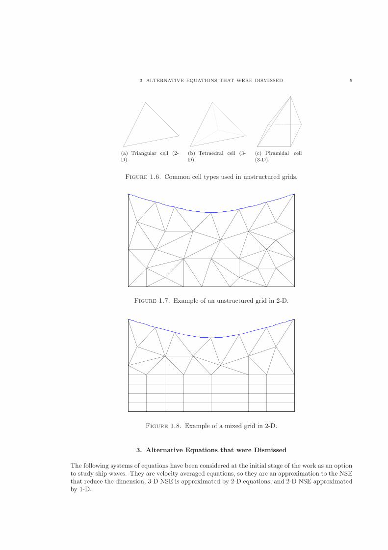
3. ALTERNATIVE EQUATIONS THAT WERE DISMISSED 5
(a) Triangular cell (2-D).
(b) Tetraedral cell (3-D).
(c) Piramidal cell(3-D).
Figure 1.6. Common cell types used in unstructured grids.
Figure 1.7. Example of an unstructured grid in 2-D.
Figure 1.8. Example of a mixed grid in 2-D.
3. Alternative Equations that were Dismissed
The following systems of equations have been considered at the initial stage of the work as an optionto study ship waves. They are velocity averaged equations, so they are an approximation to the NSEthat reduce the dimension, 3-D NSE is approximated by 2-D equations, and 2-D NSE approximatedby 1-D.
6 1. INTRODUCTION
3.1. Shallow Water Equations (SWE). SWE are depth integrated simplifications of theNSE. The vertical velocity is neglected and they can be applied where the wave length of the phe-nomenon is much bigger than the depth of the domain. They are used to model processes producedby gravitational and rotational forces and include Coriolis forces. To avoid the depth restrictionsome work has been done using more than one layer [23, 22, 64, 165].
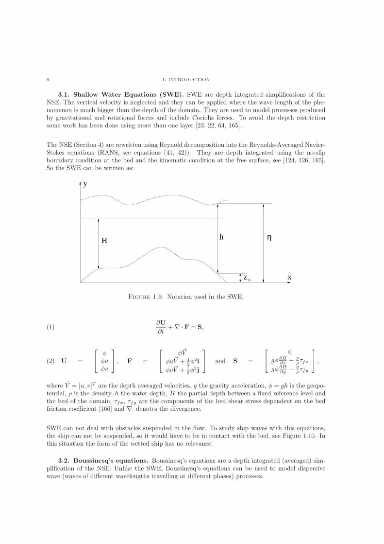
The NSE (Section 4) are rewritten using Reynold decomposition into the Reynolds-Averaged Navier-Stokes equations (RANS, see equations (41, 42)). They are depth integrated using the no-slipboundary condition at the bed and the kinematic condition at the free surface, see [124, 126, 165].So the SWE can be written as:
z b
ηhH
y
x
Figure 1.9. Notation used in the SWE.
∂U
∂t+∇ ⋅ F = S,(1)
(2) U =
⎡
⎣
��u�v
⎤
⎦ , F =
⎡
⎣
�V
�uV + 12�
2i
�vV + 12�
2j
⎤
⎦ and S =
⎡
⎣
0g�∂H
∂x − g��fx
g�∂H∂y − g
��fy
⎤
⎦ ,
where V = [u, v]T are the depth averaged velocities, g the gravity acceleration, � = gℎ is the geopo-tential, � is the density, ℎ the water depth, H the partial depth between a fixed reference level andthe bed of the domain, �fx, �fy are the components of the bed shear stress dependent on the bedfriction coefficient [166] and ∇⋅ denotes the divergence.
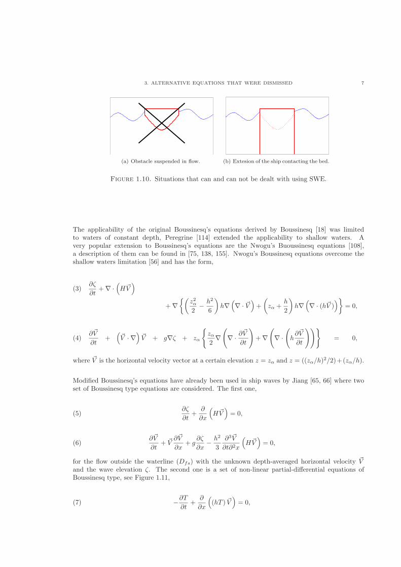
SWE can not deal with obstacles suspended in the flow. To study ship waves with this equations,the ship can not be suspended, so it would have to be in contact with the bed, see Figure 1.10. Inthis situation the form of the wetted ship has no relevance.
3.2. Boussinesq’s equations. Boussinesq’s equations are a depth integrated (averaged) sim-plification of the NSE. Unlike the SWE, Boussinesq’s equations can be used to model dispersivewave (waves of different wavelengths travelling at different phases) processes.
3. ALTERNATIVE EQUATIONS THAT WERE DISMISSED 7
(a) Obstacle suspended in flow. (b) Extesion of the ship contacting the bed.
Figure 1.10. Situations that can and can not be dealt with using SWE.
The applicability of the original Boussinesq’s equations derived by Boussinesq [18] was limitedto waters of constant depth, Peregrine [114] extended the applicability to shallow waters. Avery popular extension to Boussinesq’s equations are the Nwogu’s Buoussinesq equations [108],a description of them can be found in [75, 138, 155]. Nwogu’s Boussinesq equations overcome theshallow waters limitation [56] and has the form,
(3)∂�
∂t+∇ ⋅
(
HV)
+∇{(
z2�2
− ℎ2
6
)
ℎ∇(
∇ ⋅ V)
+
(
z� +ℎ
2
)
ℎ∇(
∇ ⋅ (ℎV ))}
= 0,
(4)∂V
∂t+
(
V ⋅ ∇)
V + g∇� + z�
{
z�2∇(
∇ ⋅ ∂V∂t
)
+∇(
∇ ⋅(
ℎ∂V
∂t
))}
= 0,
where V is the horizontal velocity vector at a certain elevation z = z� and z = ((z�/ℎ)2/2)+(z�/ℎ).
Modified Boussinesq’s equations have already been used in ship waves by Jiang [65, 66] where twoset of Boussinesq type equations are considered. The first one,
∂�
∂t+
∂
∂x
(
HV)
= 0,(5)
∂V
∂t+ V
∂V
∂x+ g
∂�
∂x− ℎ2
3
∂3V
∂t∂2x
(
HV)
= 0,(6)
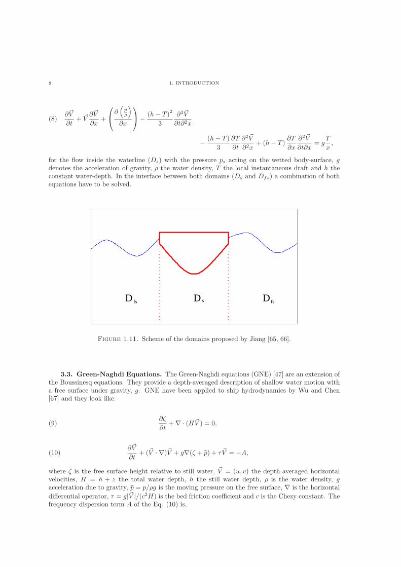
for the flow outside the waterline (Dfs) with the unknown depth-averaged horizontal velocity Vand the wave elevation �. The second one is a set of non-linear partial-differential equations ofBoussinesq type, see Figure 1.11,
−∂T∂t
+∂
∂x
(
(ℎT ) V)
= 0,(7)
8 1. INTRODUCTION
(8)∂V
∂t+ V
∂V
∂x+
⎛
⎝∂(
p�
)
∂x
⎞
⎠− (ℎ− T )2
3
∂3V
∂t∂2x
− (ℎ− T )
3
∂T
∂t
∂2V
∂2x+ (ℎ− T )
∂T
∂x
∂2V
∂t∂x= g
T
x,
for the flow inside the waterline (Ds) with the pressure ps acting on the wetted body-surface, gdenotes the acceleration of gravity, � the water density, T the local instantaneous draft and ℎ theconstant water-depth. In the interface between both domains (Ds and Dfs) a combination of bothequations have to be solved.
s D fsD fs D
Figure 1.11. Scheme of the domains proposed by Jiang [65, 66].
3.3. Green-Naghdi Equations. The Green-Naghdi equations (GNE) [47] are an extension ofthe Boussinesq equations. They provide a depth-averaged description of shallow water motion witha free surface under gravity, g. GNE have been applied to ship hydrodynamics by Wu and Chen[67] and they look like:
∂�
∂t+∇ ⋅ (HV ) = 0,(9)
∂V
∂t+ (V ⋅ ∇)V + g∇(� + p) + � V = −A,(10)
where � is the free surface height relative to still water, V = (u, v) the depth-averaged horizontalvelocities, H = ℎ + z the total water depth, ℎ the still water depth, � is the water density, gacceleration due to gravity, p = p/�g is the moving pressure on the free surface, ∇ is the horizontal
differential operator, � = g∣V ∣/(c2H) is the bed friction coefficient and c is the Chezy constant. Thefrequency dispersion term A of the Eq. (10) is,
4. NAVIER-STOKES EQUATIONS 9
(11) A = −1
6D2ℎ ⋅ ∇(2� − ℎ)
+1
6
{D2� ⋅ ∇(4� + ℎ) + (ℎ+ �) ⋅ ∇(2D2� −D2ℎ)
},
where D is the total horizontal differential operator (derivative along trajectories) with V being thevelocity of the fluid,
D =∂
∂t+ (V ⋅ ∇).(12)
4. Navier-Stokes Equations
The Navier-Stokes Equations (NSE) are a set of non-linear Partial Differential Equations (PDE)that governs the motion of viscous flows. They are named after Claude-Louis Navier and Sir GeorgeGabriel Stokes. These equations have been applied to many phenomenon in physics from hydrody-namics (water flow, ocean currents) to aerodynamics (flow around airfoils) going through meteorol-ogy (weather modelling).
The existence and smoothness of the solution of the NSE is one of the seven problems proposedby the Clay Mathematics Institute in the so-called Millennium Prize Problems. The solution ofeach problem is awarded with one million US dollars. The description of the Navier-Stokes problemproposed by the Clay Mathematics Institute is given by Fefferman [36].
“Waves follow our boat as we meander across the lake, and turbulent air currents follow our flightin a modern jet. Mathematicians and physicists believe that an explanation for and the predictionof both the breeze and the turbulence can be found through an understanding of solutions to theNSE. Although these equations were written down in the 19th Century, our understanding of themremains minimal. The challenge is to make substantial progress toward a mathematical theory whichwill unlock the secrets hidden in the NSE” [3].
4.1. Continuous Media Modelling. The fluid is a continuous material, so its properties(velocity, density, pressure) are continuous. These properties are defined at each point as the limitof volumes containing that point, for example the velocity u at point x ∈ ℝ
n, (n = 2, 3) can bedefined as,
V (x; t) = limr→0
(
1
2�r
∫
B(x,r)
V (x; t) d x
)
(13)
where B(x, r) = {y ∈ ℝn : ∣∣x− y∣∣ < r}. A similar procedure is followed to define fluid properties
(density, pressure) at every point of the fluid.
The study of physical quantities (mass and momentum) is done using representative volumes calledcontrol volume Ω. In these volumes the physical quantities are balanced over a time interval, theamount in the volume is equal to the amount leaving or entering the volume plus the amountproduced by the source, i.e.,
10 1. INTRODUCTION
(14)
(Rate of change
Inside Ω
)
=
(Flux through boundaries
Flux through ∂Ω
)
+
(SourcesInside Ω
)
.
The flux through the boundaries can be split into advection (movement with the fluid flow) anddiffusion (net transport by random, molecular or turbulent, motion).
Definition 1.1. Definitions and properties.
∙ Consider vectors a, b ∈ ℝn, the dot product is a real number defined as:
a ⋅ b = [a1, a2, . . . , an] ⋅ [b1, b2, . . . , bn] =n∑
i=1
aibi.(15)
∙ Consider a vector a = [a1, a2, . . . , an] ∈ ℝn, and another vector b = [b1, b2, . . . , bm] ∈ ℝ
m
where m can be different than n, the outer product is a n×m matrix,
a⊗ b =
⎡
⎢⎢⎢⎣
a1b1 a1b2 . . . a1bma2b1 a2b2 . . . a2bm
. . . . . .. . . . . .
anb1 anb2 . . . anbm
⎤
⎥⎥⎥⎦.(16)
∙ Consider a scalar function � : ℝ3 → ℝ The notation ∇ is used for the gradient,
∇� = grad(�) =
[∂�
∂x,∂�
∂y,∂�
∂z
]
.(17)
∙ Consider a vectorial function F : ℝ3 → ℝ3. F = [F1, F2, F3]. The notation ∇⋅ is used for
the divergence,
∇ ⋅ F = div(F ) =∂F1
∂x+∂F2
∂y+∂F3
∂z.(18)
– Consider a scalar function � : ℝ3 → ℝ and a vectorial function F : ℝ3 → ℝ3,
∇⋅︸︷︷︸
divergence
(�F ) = ( ∇︸︷︷︸
gradient
�) ⋅︸︷︷︸
dot product
F + �( ∇⋅︸︷︷︸
divergence
F )(19)
– Consider a function � : ℝ2 → ℝ and function F = [f, g] : ℝ2 → ℝ2,
(20) ∇ ⋅ (�F ⊗ F ) = ∇ ⋅[�ff �gf�fg �gg
]
=
[∂(�ff)
∂x∂(�gf)
∂y∂(�fg)
∂x∂(�gg)
∂y
]
=
[
�f ∂f∂x + f ∂�f
∂x �g ∂f∂y + f ∂�g
∂y
�f ∂g∂x + g ∂�f
∂x �g ∂g∂y + g ∂�g
∂y
]
= �
[
f ∂f∂x g ∂f
∂y
f ∂g∂x g ∂g
∂y
]
+
[
f ∂�f∂x f ∂�g
∂y
g ∂�f∂x g ∂�g
∂y
]
= �(F ⋅ ∇F ) + F∇ ⋅ (�F ).A similar procedure is applied in 3-D.
4. NAVIER-STOKES EQUATIONS 11
4.2. Conservation of Mass. When there are no sources applied to the system, the mass isconserved (density × volume = constant) [14, 152]. So the derivative along trajectories, see formula(12), is zero,
d
dt
∫
Ω
�dΩ+
∫
∂Ω
�V ⋅ ndA = 0.(21)
Applying the divergence theorem2,
d
dt
∫
Ω
�dΩ+
∫
Ω
∇ ⋅ (�V )dΩ = 0.(22)
Using Leibniz’s rule3 and asumming � and ∂�/∂t smooth, the derivative on time can be included inthe integral. Then using the fact that the integral is a scalar function4 ,
∫
Ω
(∂�
∂t+∇ ⋅ (�V )
)
dΩ = 0.(23)
The above relation has to be satisfied for every volume Ω in the fluid domain, therefore it is necessarythat the interior of the integral sign to be zero, so
∂�
∂t+∇ ⋅ (�V ) = 0.(24)
This equation is the so-called conservation of mass equation. When the flow is incompressible density(�) variations are ignored and the conservation of mass equation in this case becomes
d�
dt= 0 and ∇ ⋅ V = 0,(25)
4.3. Conservation of Momentum. For the conservation of momentum there are some forcesacting on the fluid (denoted by S) [14, 152] and equation (14) can be written as:
∫
Ω
∂(�V )
∂tdΩ+
∫
∂Ω
(�V )V ⋅ ndA =
∫
Ω
S.(26)
This equation can be integrated over volumes as the conservation of mass has been done before,obtaining
∂
∂t(�V ) +∇ ⋅ (�V ⊗ V ) + S.(27)
2Divergence theorem∫Ω ∇ ⋅ F dΩ =
∫∂Ω FndS
3Leibniz’s rule: ∂∂t
∫Ω f(x; t)dΩ =
∫Ω
∂f∂t
(x; t)dΩ.
4Scalar rule:∫Ω fdΩ+
∫Ω gdΩ =
∫Ω f + gdΩ and
∫Ω �fdΩ = �
∫Ω fdΩ for � ∈ ℝ.
12 1. INTRODUCTION
where ⊗ denotes the outer product of vectors.
Using equation (20) with � = � and F = V in equation (27) results,
(28)∂�V
∂t+ �(V ⋅ ∇V ) + V∇ ⋅ (�V ) + S = V
∂�
∂t+ �
∂V
∂t+ �(V ⋅ ∇V ) + V∇ ⋅ (�V ) + S
= V
(∂�
∂t+∇ ⋅ (�V )
)
︸ ︷︷ ︸
=0( Mass Conservation)
+�
(
∂V
∂t+ V ⋅ ∇V
)
+ S = �
(
∂V
∂t+ V ⋅ ∇V
)
+ S
Then the conservation of momentum equations states,
�
(
∂V
∂t+ V ⋅ ∇V
)
+ S = 0.(29)
The force term S can be split into two different forces, external forces Se, like gravity force, andinternal contact forces Sc.
�
(
∂V
∂t+ V ⋅ ∇V
)
+ Se + Sc = 0,(30)
The contact forces have contributions from the pressure due Johann, Bernoulli and Euler, andcontributions from viscosity due Navier and Stokes [14],
Sc = −∇p︸ ︷︷ ︸
pressure
+�∇ ⋅ V + �∇(∇ ⋅ V )︸ ︷︷ ︸
viscosity
.(31)
Where � is the viscosity coefficient and � a viscous coefficient associated with volume change whichis usually neglected.
Definition 1.2. Important CFD Parameters.
∙ Reynolds number (Re) [14] is a dimensionless parameter that provides a ratio of change inthe flow conditions depending on density ad viscosity:
Re =�LU
�,(32)
where L is a representative length, such as the maximum diameter between boundaries,U is a representative velocity, such as the velocity at the right boundary, � the density and� the viscosity.
“All those flows that satisfy the same boundary and initial conditions when expressed
in non-dimensional form (redefine V = V /U , t = t/L and x = x/L), and for which thecorresponding values of �, L, U and � are different without the value of the combination
4. NAVIER-STOKES EQUATIONS 13
�LU/� (= Re) being different, are described by one and the same non-dimensional solu-tion; and all such flows are said to be dynamically similar” [14].
The Reynolds number is the parameter indicating the character of the flow beinglaminar (the fluid travels in regular paths) or turbulent (the fluid travels in irregular andmixing paths).
∙ Mach number (M) is a dimensionless parameter that provides the ratio between thereference speed of the fluid (or obstacle in the fluid), ∣U ∣, and the speed of sound in thisfluid, cf ,
M =∣U ∣cf.(33)
Speed of sound of water at 15oC is cf = 1470m/s [14]. Like in the Reynolds number,fluids with similar Mach numbers behave alike. Flows can be classified depending on theMach number,
M
⎧
⎨
⎩
< 1 subcritical flow= 1 critical flow> 1 supercritical flow.
(34)
∙ Froude Number (Fr). The interest in this dissertation is in free surface flows, where gravityinduce the movement of the waves, in fact these kind of waves are usually called “gravitywaves”. The Froude number is a dimensionless parameter providing a ratio of inertialand gravitational forces, i.e., the ratio between the speed of the fluid (U) and the speed ofpropagation of a wave at the free surface (
√gL),
Fr = U/√
gL.(35)
The Froude number is to gravity waves the equivalent of the Mach number to gasdynamics [77], and it provides the regime of the flow in this case,
Fr
⎧
⎨
⎩
< 1 subcritical flow= 1 critical flow> 1 supercritical flow.
(36)
The NSE for incompressible flows (constant �) are called Incompressible NSE and look like,
∇ ⋅ V = 0(37)
∂V
∂t+ V ⋅ ∇V = −∇p+ �∇ ⋅ V + Se.(38)
These equations are reduced when the flow is incompressible and inviscid, resulting in the EE,
∇ ⋅ V = 0,(39)
∂V
∂t+ V ⋅ ∇V = −∇p+ Se.(40)
14 1. INTRODUCTION
A time average of the fluid properties (velocities, density and pressure) using Reynold decomposition5
is used to obtain the RANS equations, written as [113]:
∂�a∂t
+ Va ⋅ ∇�a = 0,(41)
∂�aVa∂t
+ Vb ⋅ ∇Vb = −∇pa + �a∇ ⋅ Va + Se = ∇ ⋅ (R+ S),(42)
where ub = �aua/� is the Favre average and R the Reynolds stress tensor (Ri,j = −�aub,iub,j , i, j =1, 2, 3) and uc = u− ub. This set of equations are usually applied to turbulent flows.
4.4. Artificial Compressibility Method (ACM). Using Artificial Compressibility Method(ACM) [30] the incompressible NSE are modified becoming what could be called pseudo-compressibleNSE, which is an hyperbolic system of equations. Techniques usually applied to the solution of com-pressible NSE like a Godunov-type Method can be used solving the new pseudo-compressible NSE.This method will be explained in Section 2.
5. Alternative Solution Methods
This section contains a brief revision of the methods applied not only to the NSE, but to PDE ingeneral. In the first part of the section the method used for the particular case of NSE is shown.The second part reviews the different methods for the spatial and temporal discretization in generalPDEs.
5.1. Alternative Variables. The first choice that can be made is the kind of variable used tosolve the NSE. In this study primitive variables, velocity V and pressure p are considered. That isnot the only option, “derived variables” such as the vorticity-stream variables can also be considered.
The vorticity, !, is defined as the curl of the velocity, in 3-D V = [u, v, w]T ,
! = ∇× V =
∣∣∣∣∣∣
i j k∂/∂x ∂/∂y ∂/∂zu v w
∣∣∣∣∣∣
,(43)
where i, j, k are the unitary vectors in the x, y and z directions. In two dimensions it is reducedto the z-component of this vector, i.e.,
! = ! ⋅ k =∂v
∂x− ∂u
∂y.(44)
In two dimensions a function called the stream function, , can be defined as:
∂
∂x= −v and
∂
∂y= u.(45)
5� = �a + �′ where �a denotes the average of � and �′ denotes the perturbation part.
5. ALTERNATIVE SOLUTION METHODS 15
The conservation of mass equation (37) and the conservation of momentum equation (38) can bewritten into the so-called Vorticity Equations:
Δ = −!.(46)
∂!
∂t+ (V ⋅ ∇)! = �∇ ⋅ !.(47)
The boundary conditions are difficult to implement in these variables. In addition the difficulty toextend it to 3-D makes the system not very popular in CFD.
5.2. Coupled/Uncoupled methods. Once the variables to use in the resolution of the NSEare known, the next step is the election of the way these variables are going to be considered,each one differently or both coupled. In this work the variables are coupled in a vector denotedas U. When using coupled variables the methods can be divided in direct methods or modifiedmethods. The direct methods try to solve the coupled system directly and are difficult to solve andexpensive computationally. The modified methods consist in a perturbation of the conservation ofmass equation (37) which can be done in different ways:
∙ Penalty Method, where the pressure multiplied by a penalty parameter � is added,
∇ ⋅ V = 0 ⇒ ∇ ⋅ V + �p = 0.(48)
Then the pressure can be written as p = −(∇ ⋅ V )/� and therefore the conservation ofmomentum can be written as:
∂V
∂t+ (V ⋅ ∇)V =
1
�∇(∇ ⋅ V ) + �∇ ⋅ V + Se.(49)
∙ Petrov-Galerking Method, where the perturbation has the form of the Laplacian of thepressure multiplied by a small parameter �,
∇ ⋅ V = 0 ⇒ ∇ ⋅ V − �∇ ⋅ p = 0 : ∇p ⋅ n∣∂Ω = 0.(50)
∙ ACM, the perturbation is added using a derivative of the pressure in fictitious time, � ,multiplied by an artificial compressibility parameter �. This is the method applied in thisdissertation and will be described in Section 2,
∇ ⋅ V = 0 ⇒ 1
�
∂�
∂�+∇ ⋅ V = 0.(51)
The issue in the modified methods is in choosing the value of the perturbation parameter, denotedby � in all the cases. This value has to be big enough to change the conservation of mass equationand small enough to avoid an excessive perturbation. In the case of the ACM the value of theparameter � will be discussed.
A second approach is to compute the velocity, V , and the pressure, p, in different ways. The ideais to obtain smaller systems of equations which are easier to compute. These methods are usuallycalled Projection Method or Fractional Step Methods or Predictor-Corrector Methods and wereintroduced also by Chorin in [31]. The usual methodology is:
16 1. INTRODUCTION
(1) To obtain a first estimation for the velocity V ∗ may, or may not, use a pressureapproximation,
(2) to solve a Poisson equation for the pressure6 using the estimated velocities(3) finally to update the velocity using the estimated velocity and the pressure computed.
There is a family of methods that can be considered an extension of these methods called SemiImplicitMethod for Pressure Linked Equation (SIMPLE). An iterative process is used to compute the velocityand pressure as described in [125]:
(1) Guess a pressure value p0 at each cell,
(2) obtain a first estimation for the velocity V ∗ using p0, and solving the conservation ofmomentum equation,
(3) solve a Poisson equation for the pressure using the estimated velocities and a fictitious timestep � ,
(4) correct the velocity and pressure improving the conservation of mass(5) iterate steps 2 to 4 until a divergence-free velocity field is obtained.
This method is used for example by Apsley and Hu [12], Chang and Yang [28], Ferrari et al. [38]and Wu and Hu [158].
5.3. Spatial discretization. There are different approaches for the spatial discretizationwhich are outlined in this section.
∙ Finite Difference Methods (FDM). The basic idea is to simplify the computational domainin a set of nodes and use the Taylor extension to write a discretization of the equationsbased on the neighbouring nodes.
f(x0 +Δx) = f(x0) + Δx∂f
∂x(x0) + Δx2
∂2f
∂x2(x0) +O(Δx3).(52)
Example 1.3. Lets consider the hyperbolic advection equation in 1D,
∂u
∂t+ a
∂u
∂x= 0,(53)
over a grid {xi : i = 0, 1, . . . , N}. There are different approximations to describe∂u/∂x:
– forward
(ui)x =ui+1 − ui
Δx⇒ ∂u
∂t= −aui+1 − ui
Δx(54)
– backward
(ui)x =ui − ui−1
Δx⇒ ∂u
∂t= −aui − ui−1
Δx(55)
– centred
(ui)x =ui+1 − ui−1
2Δx⇒ ∂u
∂t= −aui+1 − ui−1
2Δx.(56)
This methodology is applied to solve the NSE for example by Gerrits [43], Kleefsman[72, 73] and Veldman et al. [153].
6Poisson Equation: Δp = (∂2/∂x2 + ∂2/∂y2 + ∂2/∂z2)p = −V ⋅ ∇V
5. ALTERNATIVE SOLUTION METHODS 17
∙ Finite Element Methods (FEM). A more global approach is taken in this case. The idea isto find a finite function which approximates the solution of the NSE. The first step is torewrite the NSE in a variational form. Consider Ω the computational domain, and ∂Ω itsboundary, H1
0 (Ω) is called Sobolev space7 and is the space of smooth functions which verify
the boundary conditions. The idea is to find a function V , p ∈ H10 (Ω) such that [125],
∫
Ω
q(∇ ⋅ V )dΩ = 0, ∀q ∈ H1(Ω) :
∫
Ω
qdΩ = 0.(57)
(58)
∫
Ω
∂V
∂tv + V ⋅ ∇V vdΩ =
∫
Ω
−p∇ ⋅ v + �∇V ⋅ ∇v + Se ⋅ v, ∀v ∈ H10 (Ω).
Example 1.4. Consider the differential equation
∂2u
∂x2(x, t) = f(x), x ∈ [0, 1] u(0) = u(1) = 0.(59)
The variational equation will be,
∫
[0,1]
∂2u
∂x2(x)v(x)dx =
∫
[0,1]
f(x)v(x)dx, ∀v ∈ H10 ([0, 1]),(60)
integrating by parts and using the boundary conditions, it is obtained:
∫
[0,1]
∂u
∂x(x)
∂v
∂x(x)dx =
∫
[0,1]
f(x)v(x)dx, ∀v ∈ H10 ([0, 1]).(61)
The discretization consists of changing the scope space H10 (Ω) by a finite subset
V0 ∈ H10 (Ω) which have a basis {�i : i = 1, 2, . . . , N} of local function with compact
support8 on Ω. So every function u ∈ V0 can be written as,
u =N∑
i=1
�i�i.(62)
The Spectral Element Methods (SEM) can be considered a particular case of the FEM.In this case, instead of local compact support functions, piecewise polynomial functions areconsidered. Details about FEM and SEM can be found in [122].
These kind of methods have been applied for example by Parolini and Quarteroni [113],
Lohner et al. [85, 86, 91] and Sidlof applied FEM in [141].
∙ Finite Volume Methods (FVM). The computational domain is divided into a set of volumeswhich do not overlap each other called control volumes. The equations are integrated overthese control volumes where the fluxes are balanced at the interface between them. Theconservation properties are easily maintained both global and locally. “FVM is often seenas the most natural method for treating fluid dynamics problem” [125].
Example 1.5. Consider the hyperbolic advection equation in 1-D,
7Sobolev Space: H1(Ω) = {f ∈ L2(Ω) : ∣∣f ∣∣2 < ∞}.H1
0 (Ω) = {f ∈ H1(Ω) : f ∣∂Ω = 0}, i.e., verifies the boundary conditions.8Compact support function in Ω is a function with zero value everywhere in Ω but in a compact subset of Ω, Ω0.
18 1. INTRODUCTION
∂u
∂t+ a
∂u
∂x= 0,(63)
over a grid {xi : i = 0, 1, . . . , N}. The 1-D control volumes are {Ωi}i=1,2,...,N ={[xi−1, xi]}i=1,2,...,N . The equations are integrated over the control volumes,
∫
Ωi
∂u
∂tu(x, t)dx+ a
∫
Ωi
∂u
∂xu(x, t)dx = 0.(64)
After integration and defining ui = (1/Ωi)∫
Ωiu(x, t)dx the discretized equation results:
∂ui∂t
+ a [u(xi, t)− u(xi+1, t) = 0.](65)
The Godunov method, which can be considered a particular case of FVM, is appliedin this study, and it is described in Chapter 3.
CFX ANSYS [2], Fluent [4] are the most common commercial software applied in CFDproblems, and all of them are computed using FVM. While MIKE by DHI [5] use threedifferent methods (FDM, FEM, FVM) in the different products they have.
5.4. Temporal discretization. Temporal discretization is required in problems involving timeevolution, where the equation can be written as,
∂y
∂t= f(x, y(x)),(66)
f being a function involving or not partial derivatives of time. The different methods can be dividedinto two main categories, Explicit methods (the information at time t = tn is used to compute timet = tn+1) and Implicit methods (the calculation of time t = tn+1 is done based on the same time).
Example 1.6. Let’s consider the hyperbolic advection equation in 1-D,
∂u
∂t+ a
∂u
∂x= 0.(67)
An Explicit first order in time method can be written as:
un+1i − uni
Δt= a
uni+1 − uni−1
2Δx.(68)
A corresponding Implicit first order in time method can be written as:
un+1i − uni
Δt= a
un+1i+1 − un+1
i−1
2Δx.(69)
There are some properties which measure the method.
Definition 1.7. Definitions and properties of numerical methods [106]:
Lets denote by ℒ the operator corresponding the differential equation, so it can be written as ℒu = 0.The discrete operator is denoted by LΔt, so the discrete equation can be written as LΔtu = 0.
5. ALTERNATIVE SOLUTION METHODS 19
∙ Consistency. Defines the relation between the differential equation and the discrete scheme.A scheme is said to be consistent if
LΔtu→ ℒu, when Δt,Δx→ 0.(70)
∙ Stability. Defines the relation between the computed solution and the exact solution of thediscrete equations. Given an initial solution U0 the repetition of an action C produces theapproximation at time t = tn to be the repetition of C n-times over the initial condition U0,i.e., Un = CnU0. A scheme is said to be stable when the operator C is bounded. ConsiderK constant
∣∣Cn∣∣ < K for all n ∈ ℕ ⇔ ∣∣C∣∣ < 1.(71)
∙ Convergence. Defines the relation between the differential equation and the numericalmethod. A numerical method is said to be convergent if the numerical solution UΔt,Δx
approaches the exact solution u as the step size Δt goes to 0,
UΔt,Δx → u, when Δt,Δx→ 0.(72)
∙ Local error �n. Defines the error produced by the numerical method at time step t = tn, Un
assuming the previous steps were computed without error compared with the exact solutionat time t = tn, u(x, tn),
�n = ∣∣Un − u(x, tn)∣∣.(73)
∙ Order: The method has order p if
�n = O(ℎp) : ℎ→ 0(74)
∙ Consistency is a necessary condition for convergence, but not sufficient.
A general method which involves the most commonly used methods are called Runge-Kutta (R-K)for equation (66) can be written as [96],
ki = f(xn + ciΔt, yn +Δt
s∑
j=1
aijkj) , i = 1 . . . , s,(75)
yn+1 = yn +Δt
s∑
j=1
bjkj ,(76)
where b = {bj}sj=1, c = {cj}sj=1 ∈ ℝs and A = {aij}si,j=1 ∈ ℝ
s×s. ki are called stages and s is thenumber of stages of a method. When aij = 0 for i ≤ j the method is called explicit, if aij = 0 isonly verified for i < j the method is called semi-implicit and otherwise implicit [96].
Theorem 1.8. Existence, consistency, stability and order [96].
∙ Lets consider f Lipschitz9 with constant L and ℎ∗L∣∣A∣∣∞ < 1. Then the R-K given byequations (75,76) has unique solution for all ℎ ∈ (0, ℎ∗].
∙ A R-K given by equations (75,76) is consistent if and only if b1 + . . .+ bs = 1
9f(x) is a Lipschitz function in Ω if there exist a constant L such that: ∣∣f(x1)−f(x2)∣∣ < L∣∣x1−x2∣∣ for all x1, x2 ∈ Ω.
20 1. INTRODUCTION
∙ Lets consider ℎ∗L∣∣A∣∣∞ < 1, then the R-K given by equations (75,76) is stable for allℎ ∈ (0, ℎ∗].
∙ A R-K method given by equations (75,76) of s stages can achieve a maximum order of s.
The most common R-K methods used are:
∙ Explicit first order, also called forward Euler, is a first order one stage method with c1 = 0,a1,1 = 0 and b1 = 1.
∙ Explicit Euler modified is a second order two stage method with b1 = c1 = a1,1 = a1,2 = 0,and a2,1 = 1/2, a2,2 = 0., b2 = 1, c2 = 1.2.
∙ Explicit Euler improved is a second order two stage method with b1 = 1/2, c1 = a1,1 =a1,2 = 0, and a2,1 = 1, a2,2 = 0, b2 = 1/2, c2 = 0.
∙ Explicit Heun’s method is a second order two stage method with b1 = 1/4, c1 = a1,1 =a1,2 = 0, and a2,1 = 2/3, a2,2 = 0., b2 = 3/4, c2 = 2/3.
∙ Implicit first order, also called backward Euler, is a first order one stage method withc1 = 1, a1,1 = 1 and b1 = 1.
∙ Explicit fourth order method and the most popular therefore called R-K “withoutsurnames” is a fourth order four stages method with the following non-zero values ofA, b, c: c2 = 1/2, c3 = 1/2, c4 = 1, a21 = 1/2, a32 = 1/2, a43 = 1, b1 = 1/6, b2 = 2/6,b3 = 2/6 and b4 = 1/6.
5.5. Lattice Methods. Instead of studding what happens in a grid covering the domain, aLattice is defined in the domain. Particles (with no mass) are located at the vertex of the Lat-tice and move through it. The original method was the Lattice Gas Automata (LGA) in the late1980’s. The Lattice Boltmann Method (LBM) [55] is used to simulate flow building a simplifiedkinetic mesoscopic (the scale is big enough to not consider the behaviour of individual atoms) modelincorporating the physics of the macroscopic (scale bigger than 1mm) averaged properties of theNSE [10]. This method is gaining popularity because it is very flexible to describe complicatedboundaries and interactions among different fluids (free surface problems). A detailed descriptionof this method can be found in [10, 74, 144, 154]
(a) Rectangular Lattice in the domain. (b) Possibilities of movement fora particle in a rectangular Lattice(D2Q9).
Figure 1.12. Lattice Boltzmann Method.
The classic form of a LBM is to solve a equation,
Df = J(f),(77)
5. ALTERNATIVE SOLUTION METHODS 21
where f(t;x; V ) is a particle density function depending on time t, position x and velocity at that
position and time V (t;x). This method comprises two steps, one is the transport step (left handside, LHS) and the other is the collision step (right hand side, RHS). The collision operator J canhave different forms, depending on the considered approximation. Using the Bhatnagar-Gross-Krook(LBM-BGK) [50] it has the form,
J(f) = −1
�(f − feq),(78)
where � is a relaxation parameter related with the viscosity, and feq is the equilibrium particledensity.
In the LBM particles move from one vertex of the Lattice to the next one, which is a problemwhen the vertex of the Lattice changes position, as in the case of free surface problems. LBM alsointroduce some numerical instabilities in the truncation of the equilibrium density [92].
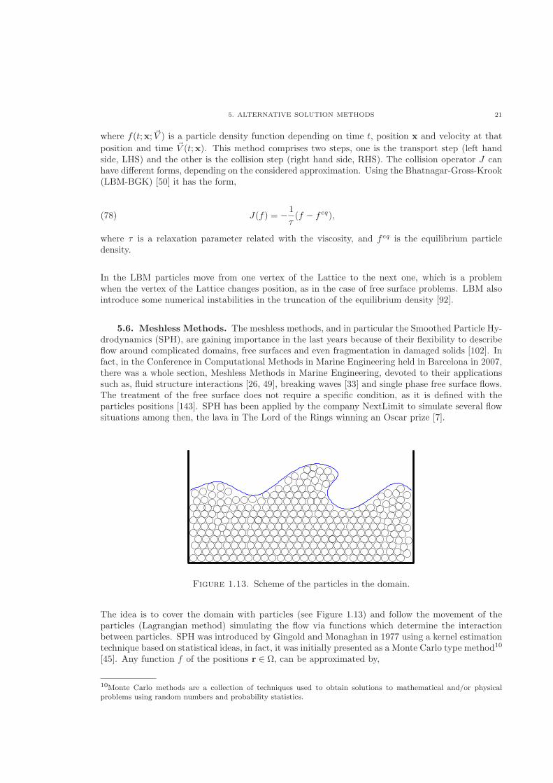
5.6. Meshless Methods. The meshless methods, and in particular the Smoothed Particle Hy-drodynamics (SPH), are gaining importance in the last years because of their flexibility to describeflow around complicated domains, free surfaces and even fragmentation in damaged solids [102]. Infact, in the Conference in Computational Methods in Marine Engineering held in Barcelona in 2007,there was a whole section, Meshless Methods in Marine Engineering, devoted to their applicationssuch as, fluid structure interactions [26, 49], breaking waves [33] and single phase free surface flows.The treatment of the free surface does not require a specific condition, as it is defined with theparticles positions [143]. SPH has been applied by the company NextLimit to simulate several flowsituations among then, the lava in The Lord of the Rings winning an Oscar prize [7].
Figure 1.13. Scheme of the particles in the domain.
The idea is to cover the domain with particles (see Figure 1.13) and follow the movement of theparticles (Lagrangian method) simulating the flow via functions which determine the interactionbetween particles. SPH was introduced by Gingold and Monaghan in 1977 using a kernel estimationtechnique based on statistical ideas, in fact, it was initially presented as a Monte Carlo type method10
[45]. Any function f of the positions r ∈ Ω, can be approximated by,
10Monte Carlo methods are a collection of techniques used to obtain solutions to mathematical and/or physicalproblems using random numbers and probability statistics.
22 1. INTRODUCTION
⟨f(r)⟩ =∫
Ω
f(r′)W (∣r− r′∣, ℎ)dr′,(79)
where Ω is the whole computational domain, W is the kernel function depending on the distancebetween particles and ℎ is a distance called the smoothing length [143]. “The kernels are functionswhich tend to the delta function as the length scale h tends to zero . . . The most commonly usedkernels are based on Schoenberg Mn splines which are piece-wise continuous functions with compactsupport having the derivatives up to (n-2) continuous” [102].
Consider N the number of particles {i : i = 1, 2, . . . , N} in the domain, this equation can bediscretized as [102, 143],
⟨f(ri)⟩ =N∑
j=1
f(rj)W (∣ri − rj ∣, ℎ)Ωj ,(80)
Ωj being the volume associated to particle j and rj its position. These techniques are used to write“SPH-versions of the NSE” to simulate flow problems. The spatial derivatives of function f canbe written as function of the derivatives of the kernel which has the information about the spatialapproximations. For a generic particle i the conservation of mass equation looks like [143],
∂�i∂t
=
N∑
j=1
mj(Vi − Vj)∇W (∣ri − rj ∣, ℎ),(81)
where mj is the mass of particle j (m = �V ) and Vj denotes the velocity of particle j and theconservation of momentum holds,
∂Vi∂t
= −N∑
j=1
mj
(
Pi
�2i+Pj
�2j+Πi,j
)
∇W (∣ri − rj ∣, ℎ) + g,(82)
Pj being the pressure in particle j. Different viscous terms Πij can be considered, for example in[143] this term has the following form,
Πi,j = −�cs�i,j
�i,jand �ij =
ℎ(Vi − Vj)(ri − rj)
(ri − rj)2 + �2(83)
�ij being the averaged density of particles i and j, cs the numerical sound speed, � the viscosityparameter and � a relaxation parameter to avoid singularities when (ri − rj) → 0 [143].
The SPH method was introduced for self-gravity gases and it is being adapted to gravity flows,therefore SPH still needs investigation in the treatment of the free surfaces, solid boundaries and tomodel the effects of viscosity [143].
6. OUTLINE OF THE THESIS 23
6. Outline of the Thesis
In this introductory Chapter the motivation of this dissertation has been explained and a brief de-scription of the techniques used in this study has been given. Also a revision of alternative griddingmethods (Section 2), equations to be used (Section 3), the NSE (Section 4) and solution methods(Section 5) has been introduced.
Chapter 2 contains a detailed description of the CCCM used at the CMMFA. The method involvesa merging cells technique to avoid very small cell numerical stability errors unless an unrealisticallysmall time step is considered. The CCCR used in this work are described in this Chapter.
In Chapter 3 the methodology used to solve the NSE are explained. The ACM and Godunov-typemethods are described together with the importance of the RP and different solvers for it.
Once the grid and the solver for the equation are described, the movement of the free surface is ex-plained in Chapter 4. A detailed description of the methods used in the bibliography is given. TheHeight Function Method applied in this study and the fourth order R-K applied for its integrationare given.
The numerical experiments are divided into two groups. Chapter 5 contains experiments withoutfree surface, as the lid-driven Couette flow, the lid-driven Cavity flow, and flow in a pipe with andwithout obstacle. Numerical experiments involving the movement of the free surface are tested inChapter 6, like the small amplitude sloshing tank, the mass-wave maker, the semi-dam break andthe current passing different obstacles (bump (CFPOB) and body(CFPCBF)). The idea suggestedin this dissertation to approximate ship generated waves is also shown in the last experiment of thisChapter, current flow passing a cylinder at the free surface (CFPCFS).
The conclusions obtained from this research and ideas for future works are highlighted in Chapter7.

CHAPTER 2
Cartesian Cut Cell Method
1. Introduction
The Cartesian Cut Cell Method (CCCM) is applied to define the computational domain where theequations should be solved. The basic idea of this method is to cover the initial domain with a Carte-sian grid. Over this initial grid solid bodies are placed. The initial grid is adapted to the solid bodyby cuts over its cells. When the solid body moves, only the affected cells need to be re-cut, avoidingto recompute again the whole grid. The method used is explained in detail in [24, 25, 63, 126, 162]for the 2-D version and in [161] for the 3-D version.
The CCCM has been used at the CMMFD to define the grid around obstacles (static or moving ata predefined velocity) in the flow, and this is the first time the method is used to define the gridaround the free surface. The movement of the free surface is unknown a priori and the boundaryconditions are different that in the case of solid obstacles.
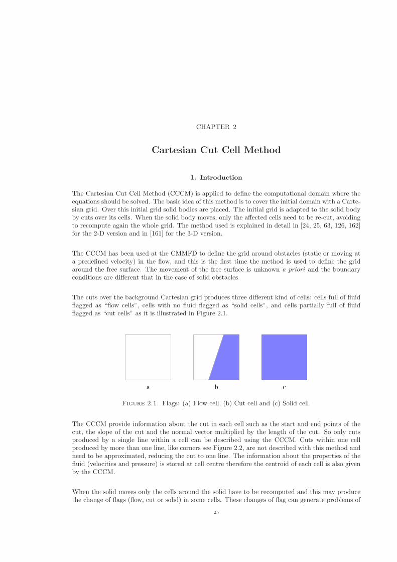
The cuts over the background Cartesian grid produces three different kind of cells: cells full of fluidflagged as “flow cells”, cells with no fluid flagged as “solid cells”, and cells partially full of fluidflagged as “cut cells” as it is illustrated in Figure 2.1.
b ca
Figure 2.1. Flags: (a) Flow cell, (b) Cut cell and (c) Solid cell.
The CCCM provide information about the cut in each cell such as the start and end points of thecut, the slope of the cut and the normal vector multiplied by the length of the cut. So only cutsproduced by a single line within a cell can be described using the CCCM. Cuts within one cellproduced by more than one line, like corners see Figure 2.2, are not described with this method andneed to be approximated, reducing the cut to one line. The information about the properties of thefluid (velocities and pressure) is stored at cell centre therefore the centroid of each cell is also givenby the CCCM.
When the solid moves only the cells around the solid have to be recomputed and this may producethe change of flags (flow, cut or solid) in some cells. These changes of flag can generate problems of
25
26 2. CARTESIAN CUT CELL METHOD
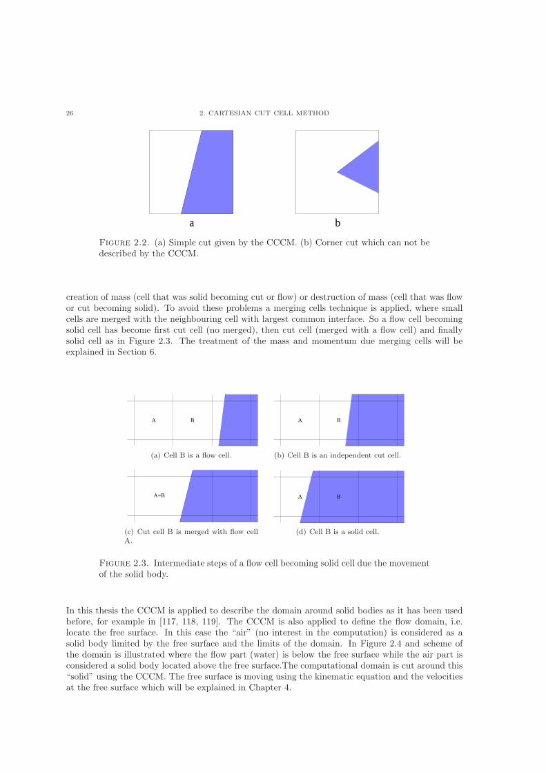
a b
Figure 2.2. (a) Simple cut given by the CCCM. (b) Corner cut which can not bedescribed by the CCCM.
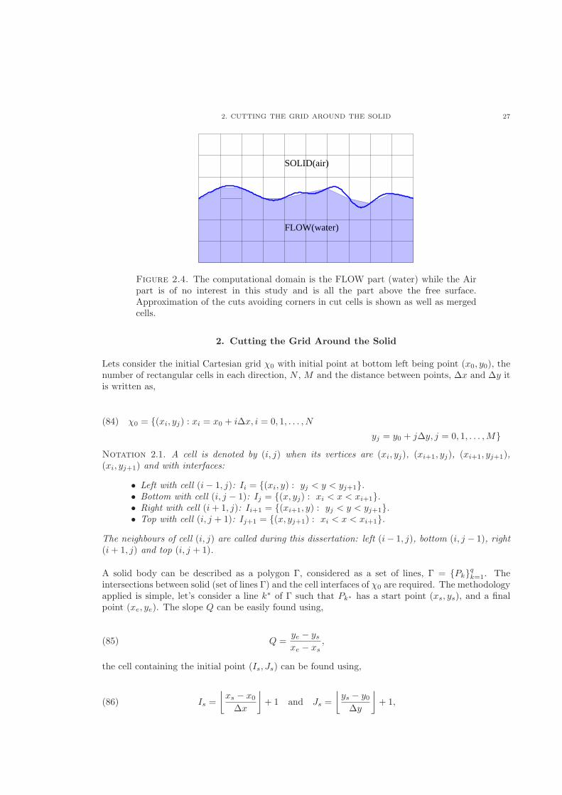
creation of mass (cell that was solid becoming cut or flow) or destruction of mass (cell that was flowor cut becoming solid). To avoid these problems a merging cells technique is applied, where smallcells are merged with the neighbouring cell with largest common interface. So a flow cell becomingsolid cell has become first cut cell (no merged), then cut cell (merged with a flow cell) and finallysolid cell as in Figure 2.3. The treatment of the mass and momentum due merging cells will beexplained in Section 6.
A B
(a) Cell B is a flow cell.
A B
(b) Cell B is an independent cut cell.
A=B
(c) Cut cell B is merged with flow cellA.
A B
(d) Cell B is a solid cell.
Figure 2.3. Intermediate steps of a flow cell becoming solid cell due the movementof the solid body.
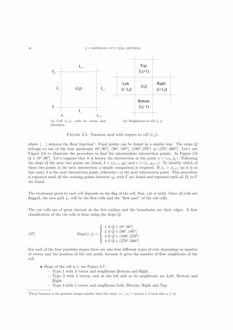
In this thesis the CCCM is applied to describe the domain around solid bodies as it has been usedbefore, for example in [117, 118, 119]. The CCCM is also applied to define the flow domain, i.e.locate the free surface. In this case the “air” (no interest in the computation) is considered as asolid body limited by the free surface and the limits of the domain. In Figure 2.4 and scheme ofthe domain is illustrated where the flow part (water) is below the free surface while the air part isconsidered a solid body located above the free surface.The computational domain is cut around this“solid” using the CCCM. The free surface is moving using the kinematic equation and the velocitiesat the free surface which will be explained in Chapter 4.
2. CUTTING THE GRID AROUND THE SOLID 27
FLOW(water)
SOLID(air)
Figure 2.4. The computational domain is the FLOW part (water) while the Airpart is of no interest in this study and is all the part above the free surface.Approximation of the cuts avoiding corners in cut cells is shown as well as mergedcells.
2. Cutting the Grid Around the Solid
Lets consider the initial Cartesian grid �0 with initial point at bottom left being point (x0, y0), thenumber of rectangular cells in each direction, N , M and the distance between points, Δx and Δy itis written as,
(84) �0 = {(xi, yj) : xi = x0 + iΔx, i = 0, 1, . . . , N
yj = y0 + jΔy, j = 0, 1, . . . ,M}
Notation 2.1. A cell is denoted by (i, j) when its vertices are (xi, yj), (xi+1, yj), (xi+1, yj+1),(xi, yj+1) and with interfaces:
∙ Left with cell (i− 1, j): Ii = {(xi, y) : yj < y < yj+1}.∙ Bottom with cell (i, j − 1): Ij = {(x, yj) : xi < x < xi+1}.∙ Right with cell (i+ 1, j): Ii+1 = {(xi+1, y) : yj < y < yj+1}.∙ Top with cell (i, j + 1): Ij+1 = {(x, yj+1) : xi < x < xi+1}.
The neighbours of cell (i, j) are called during this dissertation: left (i− 1, j), bottom (i, j − 1), right(i+ 1, j) and top (i, j + 1).
A solid body can be described as a polygon Γ, considered as a set of lines, Γ = {Pk}qk=1. Theintersections between solid (set of lines Γ) and the cell interfaces of �0 are required. The methodologyapplied is simple, let’s consider a line k∗ of Γ such that Pk∗ has a start point (xs, ys), and a finalpoint (xe, ye). The slope Q can be easily found using,
Q =ye − ysxe − xs
,(85)
the cell containing the initial point (Is, Js) can be found using,
Is =
⌊xs − x0Δx
⌋
+ 1 and Js =
⌊ys − y0Δy
⌋
+ 1,(86)
28 2. CARTESIAN CUT CELL METHOD
x x
y
y
I
I
I
I
j
j+1
i i+1
i i+1
j
j+1
(i,j)
(a) Cell (i, j), with its vertex and
interfaces.
(i,j+1)
(i+1,j)(i−1,j)
(i,j−1)
(i,j)Left
Top
Right
Bottom
(b) Neighbours of cell (i, j).
Figure 2.5. Notation used with respect to cell (i, j).
where ⌊ ⌋ denotes the floor function1. Final points can be found in a similar way. The slope Qbelongs to one of the four quadrants (0o, 90o], (90o, 180o], (180o, 270o] or (270o, 360o]. Let’s useFigure 2.6 to illustrate the procedure to find the intermediate intersection points. In Figure 2.6Q ∈ (0o, 90o]. Let’s suppose that it is known the intersection at the point a = (xa, yj). Followingthe slope Q the next two points are found, b = (xi+1, yb) and c = (xc, yj+1). To identify which ofthese two points is the next intersection a simple comparison is required. If xc > xi+1 (as it is inthis case), b is the next intersection point, otherwise c is the next intersection point. This procedureis repeated until all the crossing points between �0 with Γ are found and repeated until all Pk in Γare found.
The treatment given to each cell depends on the flag of the cell, flow, cut or solid. Once all cells areflagged, the new grid �1 will be the flow cells and the “flow part” of the cut cells.
The cut cells are of great interest as the free surface and the boundaries are their edges. A firstclassification of the cut cells is done using the slope Q,
Slope(i, j) =
⎧
⎨
⎩
1 if Q ∈ (0o, 90o]2 if Q ∈ (90o, 180o]3 if Q ∈ (180o, 270o]4 if Q ∈ (270o, 360o]
(87)
For each of the four possibles slopes there are also four different types of cuts depending on numberof vertex and the position of the exit point, because it gives the number of flow neighbours of thecell.
∙ Slope of the cell is 1, see Figure 2.7.– Type 1 with 3 vertex and neighbours Bottom and Right.– Type 2 with 4 vertex, exit at the left side so its neighbours are Left, Bottom and
Right.– Type 3 with 5 vertex and neighbours Left, Bottom, Right and Top.
1Floor function is the greatest integer smaller than the value, i.e., ⌊x⌋ = max{n ∈ ℤ such that n ≤ x}
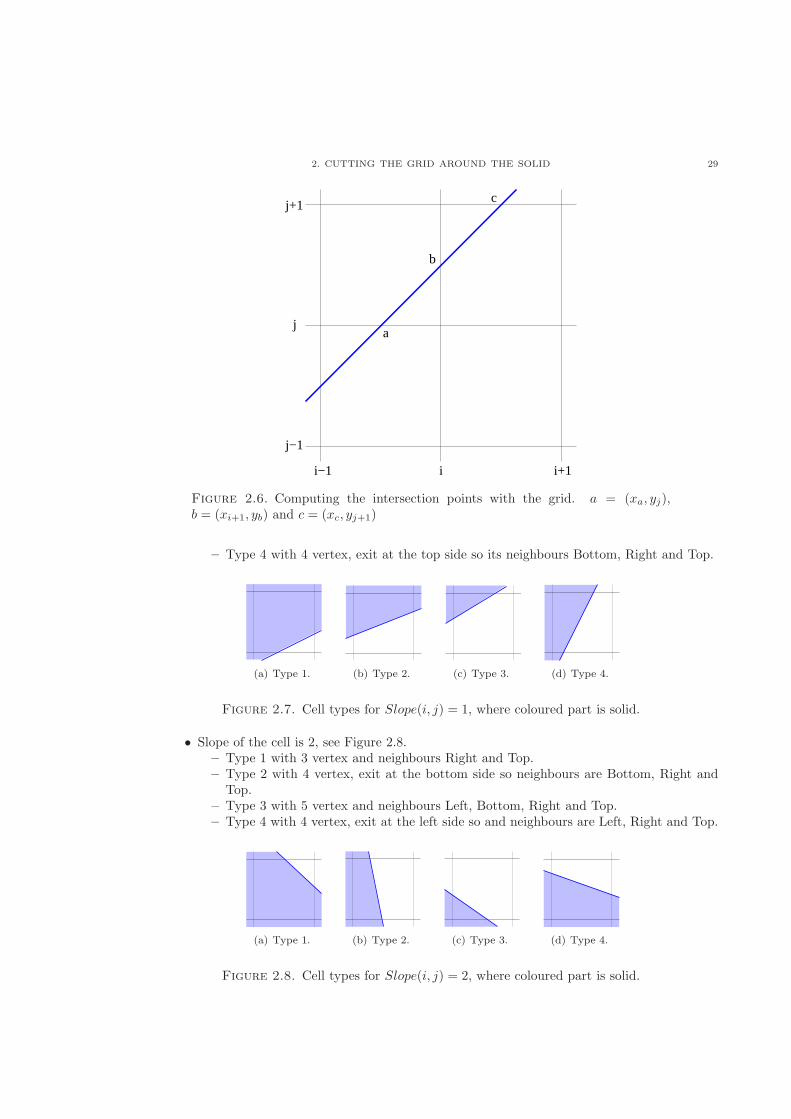
2. CUTTING THE GRID AROUND THE SOLID 29
a
b
cj+1
j
j−1
ii−1 i+1
Figure 2.6. Computing the intersection points with the grid. a = (xa, yj),b = (xi+1, yb) and c = (xc, yj+1)
– Type 4 with 4 vertex, exit at the top side so its neighbours Bottom, Right and Top.
(a) Type 1. (b) Type 2. (c) Type 3. (d) Type 4.
Figure 2.7. Cell types for Slope(i, j) = 1, where coloured part is solid.
∙ Slope of the cell is 2, see Figure 2.8.– Type 1 with 3 vertex and neighbours Right and Top.– Type 2 with 4 vertex, exit at the bottom side so neighbours are Bottom, Right and
Top.– Type 3 with 5 vertex and neighbours Left, Bottom, Right and Top.– Type 4 with 4 vertex, exit at the left side so and neighbours are Left, Right and Top.
(a) Type 1. (b) Type 2. (c) Type 3. (d) Type 4.
Figure 2.8. Cell types for Slope(i, j) = 2, where coloured part is solid.
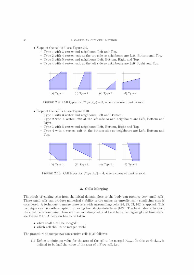
30 2. CARTESIAN CUT CELL METHOD
∙ Slope of the cell is 3, see Figure 2.9.– Type 1 with 3 vertex and neighbours Left and Top.– Type 2 with 4 vertex, exit at the top side so neighbours are Left, Bottom and Top.– Type 3 with 5 vertex and neighbours Left, Bottom, Right and Top.– Type 4 with 4 vertex, exit at the left side so neighbours are Left, Right and Top.
(a) Type 1. (b) Type 2. (c) Type 3. (d) Type 4.
Figure 2.9. Cell types for Slope(i, j) = 3, where coloured part is solid.
∙ Slope of the cell is 4, see Figure 2.10.– Type 1 with 3 vertex and neighbours Left and Bottom.– Type 2 with 4 vertex, exit at the left side so and neighbours are Left, Bottom and
Right.– Type 3 with 5 vertex and neighbours Left, Bottom, Right and Top.– Type 4 with 4 vertex, exit at the bottom side so neighbours are Left, Bottom and
Top.
(a) Type 1. (b) Type 2. (c) Type 3. (d) Type 4.
Figure 2.10. Cell types for Slope(i, j) = 4, where coloured part is solid.
3. Cells Merging
The result of cutting cells from the initial domain close to the body can produce very small cells.These small cells can produce numerical stability errors unless an unrealistically small time step isconsidered. A technique to merge these cells with surroundings cells [24, 25, 63, 162] is applied. Thistechnique can be easily adapted to moving boundaries/interfaces [163]. The basic idea is to avoidthe small cells combining them with surroundings cell and be able to use bigger global time steps,see Figure 2.11. A decision has to be taken:
∙ when shall a cell be merged?∙ which cell shall it be merged with?
The procedure to merge two consecutive cells is as follows:
(1) Define a minimum value for the area of the cell to be merged Amin. In this work Amin isdefined to be half the value of the area of a Flow cell, i.e.,
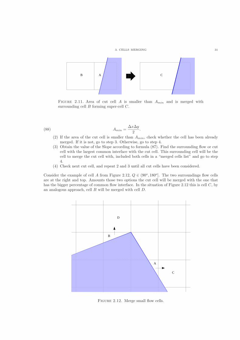
3. CELLS MERGING 31
������������������������������������
������������������������������������
B A C
Figure 2.11. Area of cut cell A is smaller than Amin and is merged withsurrounding cell B forming super-cell C.
Amin =ΔxΔy
2.(88)
(2) If the area of the cut cell is smaller than Amin, check whether the cell has been alreadymerged. If it is not, go to step 3. Otherwise, go to step 4.
(3) Obtain the value of the Slope according to formula (87). Find the surrounding flow or cutcell with the largest common interface with the cut cell. This surrounding cell will be thecell to merge the cut cell with, included both cells in a “merged cells list” and go to step4.
(4) Check next cut cell, and repeat 2 and 3 until all cut cells have been considered.
Consider the example of cell A from Figure 2.12, Q ∈ (90o, 180o]. The two surroundings flow cellsare at the right and top. Amounts those two options the cut cell will be merged with the one thathas the bigger percentage of common flow interface. In the situation of Figure 2.12 this is cell C, byan analogous approach, cell B will be merged with cell D.
������
������
����
����
A
C
B
D
Figure 2.12. Merge small flow cells.
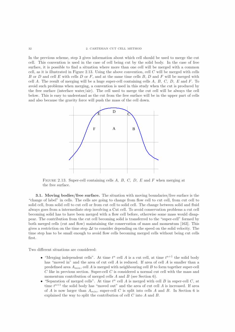
32 2. CARTESIAN CUT CELL METHOD
In the previous scheme, step 3 gives information about which cell should be used to merge the cutcell. This convention is used in the case of cell being cut by the solid body. In the case of freesurface, it is possible to find a situation where more than one cell will be merged with a commoncell, as it is illustrated in Figure 2.13. Using the above convention, cell C will be merged with cellsB or D and cell E with cells D or F , and at the same time cells B, D and F will be merged withcell A. The result of merging will be a huge super-cell containing cells A, B, C, D, E and F . Toavoid such problems when merging, a convention is used in this study when the cut is produced bythe free surface (interface water/air). The cell used to merge the cut cell will be always the cellbelow. This is easy to understand as the cut from the free surface will be in the upper part of cellsand also because the gravity force will push the mass of the cell down.
A BF
DE C
Figure 2.13. Super-cell containing cells A, B, C, D, E and F when merging atthe free surface.
3.1. Moving bodies/free surface. The situation with moving boundaries/free surface is the“change of label” in cells. The cells are going to change from flow cell to cut cell, from cut cell tosolid cell, from solid cell to cut cell or from cut cell to solid cell. The change between solid and fluidalways goes from a intermediate step involving a Cut cell. To avoid conservation problems a cut cellbecoming solid has to have been merged with a flow cell before, otherwise some mass would disap-pear. The contribution from the cut cell becoming solid is transferred to the “super-cell” formed byboth merged cells (cut and flow) maintaining the conservation of mass and momentum [163]. Thisgives a restriction on the time step Δt to consider depending on the speed on the solid velocity. Thetime step has to be small enough to avoid flow cells becoming merged cells without being cut cellsfirst.
Two different situations are considered:
∙ “Merging independent cells”. At time tn cell A is a cut cell, at time tn+1 the solid bodyhas “moved in” and the area of cut cell A is reduced. If area of cell A is smaller than apredefined area Amin, cell A is merged with neighbouring cell B to form together super-cellC like in previous section. Super-cell C is considered a normal cut cell with the mass andmomentum contribution of merged cells A and B (see Section 6).
∙ “Separation of merged cells”. At time tn cell A is merged with cell B in super-cell C, attime tn+1 the solid body has “moved out” and the area of cut cell A is increased. If areaof A is now larger than Amin, super-cell C is split into cells A and B. In Section 6 isexplained the way to split the contribution of cell C into A and B.
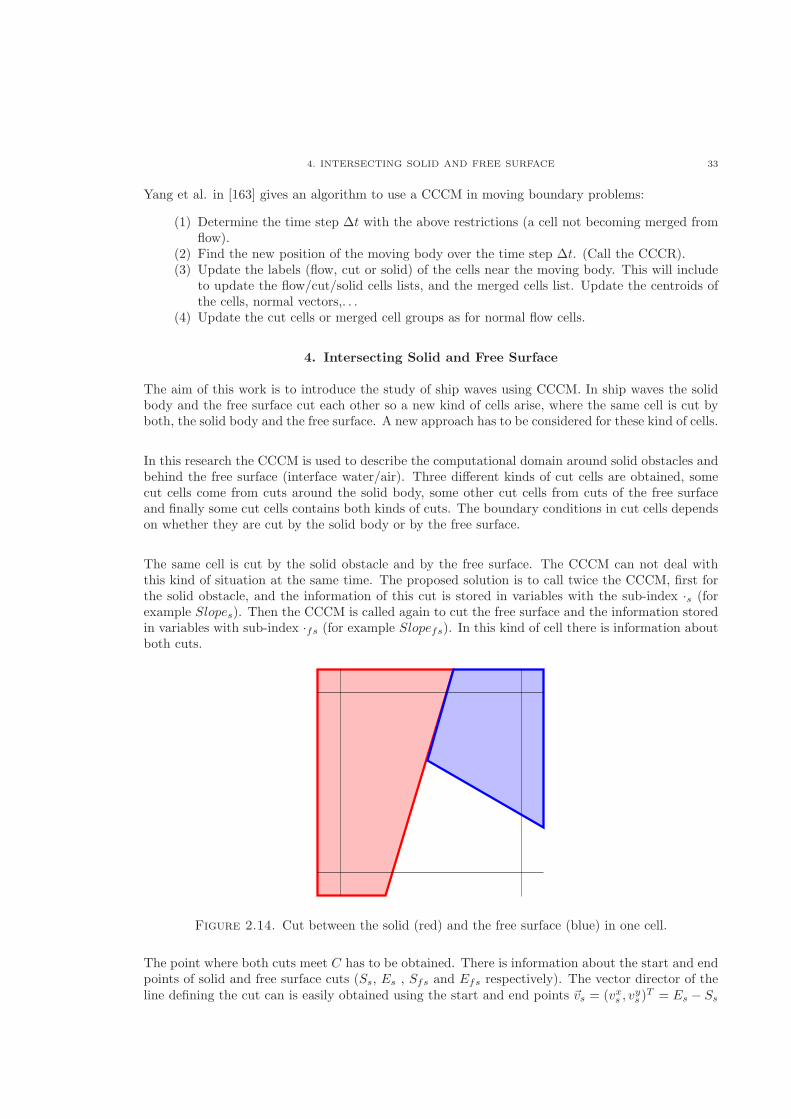
4. INTERSECTING SOLID AND FREE SURFACE 33
Yang et al. in [163] gives an algorithm to use a CCCM in moving boundary problems:
(1) Determine the time step Δt with the above restrictions (a cell not becoming merged fromflow).
(2) Find the new position of the moving body over the time step Δt. (Call the CCCR).(3) Update the labels (flow, cut or solid) of the cells near the moving body. This will include
to update the flow/cut/solid cells lists, and the merged cells list. Update the centroids ofthe cells, normal vectors,. . .
(4) Update the cut cells or merged cell groups as for normal flow cells.
4. Intersecting Solid and Free Surface
The aim of this work is to introduce the study of ship waves using CCCM. In ship waves the solidbody and the free surface cut each other so a new kind of cells arise, where the same cell is cut byboth, the solid body and the free surface. A new approach has to be considered for these kind of cells.
In this research the CCCM is used to describe the computational domain around solid obstacles andbehind the free surface (interface water/air). Three different kinds of cut cells are obtained, somecut cells come from cuts around the solid body, some other cut cells from cuts of the free surfaceand finally some cut cells contains both kinds of cuts. The boundary conditions in cut cells dependson whether they are cut by the solid body or by the free surface.
The same cell is cut by the solid obstacle and by the free surface. The CCCM can not deal withthis kind of situation at the same time. The proposed solution is to call twice the CCCM, first forthe solid obstacle, and the information of this cut is stored in variables with the sub-index ⋅s (forexample Slopes). Then the CCCM is called again to cut the free surface and the information storedin variables with sub-index ⋅fs (for example Slopefs). In this kind of cell there is information aboutboth cuts.
Figure 2.14. Cut between the solid (red) and the free surface (blue) in one cell.
The point where both cuts meet C has to be obtained. There is information about the start and endpoints of solid and free surface cuts (Ss, Es , Sfs and Efs respectively). The vector director of theline defining the cut can is easily obtained using the start and end points vs = (vxs , v
ys )
T = Es − Ss
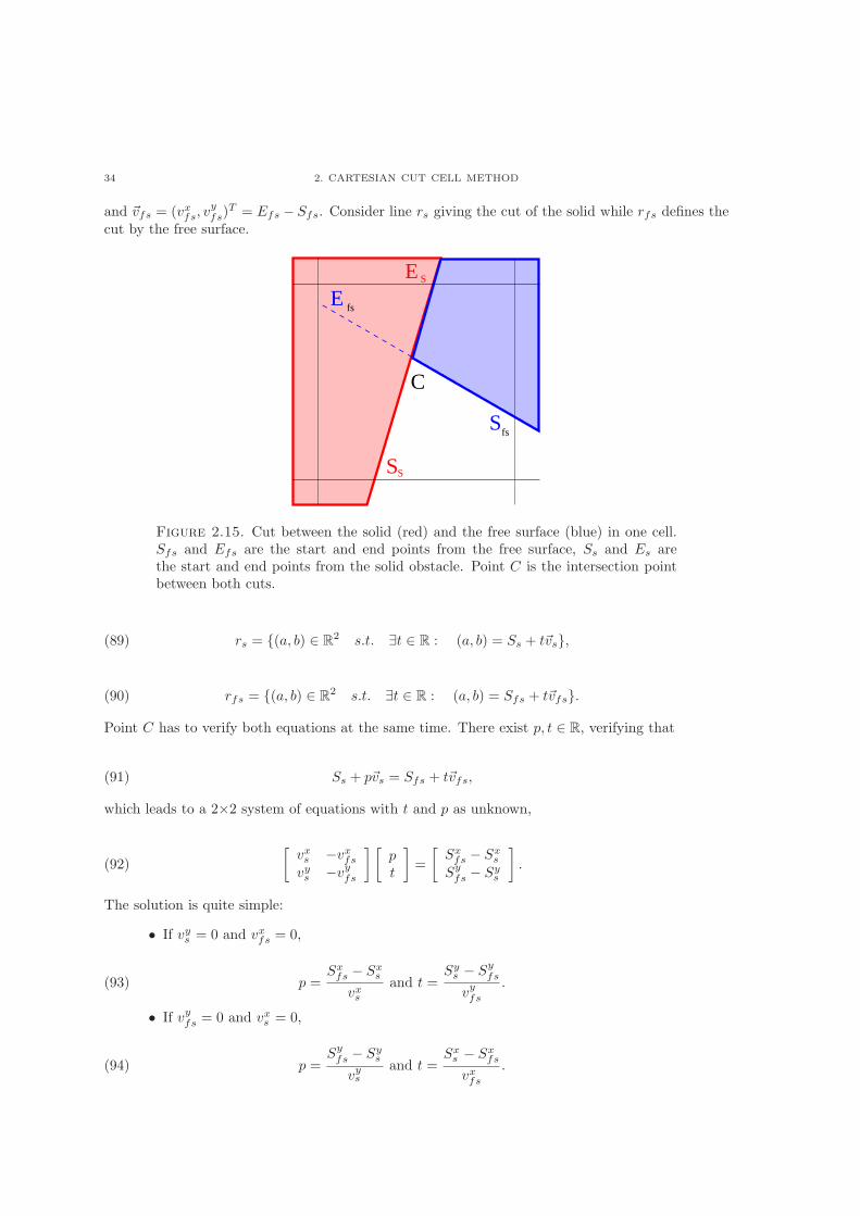
34 2. CARTESIAN CUT CELL METHOD
and vfs = (vxfs, vyfs)
T = Efs − Sfs. Consider line rs giving the cut of the solid while rfs defines thecut by the free surface.
C
E fs
ES
Sfs
SS
Figure 2.15. Cut between the solid (red) and the free surface (blue) in one cell.Sfs and Efs are the start and end points from the free surface, Ss and Es arethe start and end points from the solid obstacle. Point C is the intersection pointbetween both cuts.
rs = {(a, b) ∈ ℝ2 s.t. ∃t ∈ ℝ : (a, b) = Ss + tvs},(89)
rfs = {(a, b) ∈ ℝ2 s.t. ∃t ∈ ℝ : (a, b) = Sfs + tvfs}.(90)
Point C has to verify both equations at the same time. There exist p, t ∈ ℝ, verifying that
Ss + pvs = Sfs + tvfs,(91)
which leads to a 2×2 system of equations with t and p as unknown,
[vxs −vxfsvys −vyfs
] [pt
]
=
[Sxfs − Sx
s
Syfs − Sy
s
]
.(92)
The solution is quite simple:
∙ If vys = 0 and vxfs = 0,
p =Sxfs − Sx
s
vxsand t =
Sys − Sy
fs
vyfs.(93)
∙ If vyfs = 0 and vxs = 0,
p =Syfs − Sy
s
vysand t =
Sxs − Sx
fs
vxfs.(94)
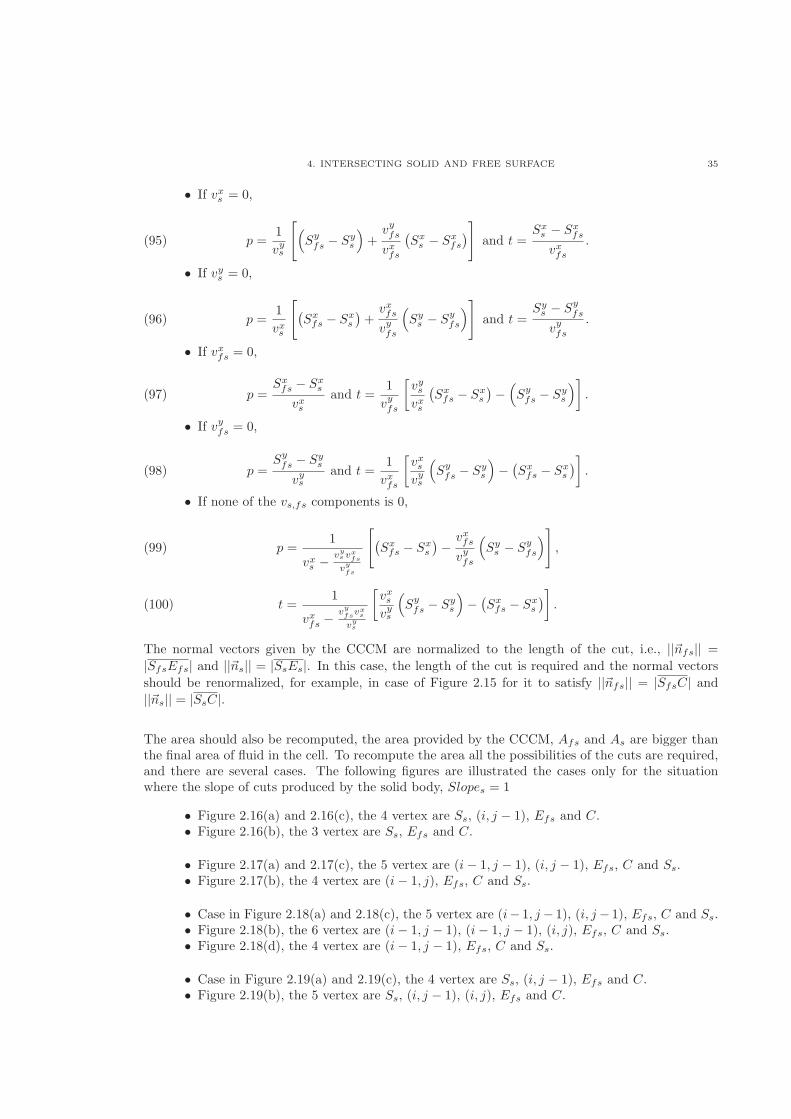
4. INTERSECTING SOLID AND FREE SURFACE 35
∙ If vxs = 0,
p =1
vys
[(
Syfs − Sy
s
)
+vyfsvxfs
(Sxs − Sx
fs
)
]
and t =Sxs − Sx
fs
vxfs.(95)
∙ If vys = 0,
p =1
vxs
[
(Sxfs − Sx
s
)+vxfsvyfs
(
Sys − Sy
fs
)]
and t =Sys − Sy
fs
vyfs.(96)
∙ If vxfs = 0,
p =Sxfs − Sx
s
vxsand t =
1
vyfs
[vysvxs
(Sxfs − Sx
s
)−(
Syfs − Sy
s
)]
.(97)
∙ If vyfs = 0,
p =Syfs − Sy
s
vysand t =
1
vxfs
[vxsvys
(
Syfs − Sy
s
)
−(Sxfs − Sx
s
)]
.(98)
∙ If none of the vs,fs components is 0,
p =1
vxs − vys v
xfs
vy
fs
[
(Sxfs − Sx
s
)−vxfsvyfs
(
Sys − Sy
fs
)]
,(99)
t =1
vxfs −vy
fsvxs
vys
[vxsvys
(
Syfs − Sy
s
)
−(Sxfs − Sx
s
)]
.(100)
The normal vectors given by the CCCM are normalized to the length of the cut, i.e., ∣∣nfs∣∣ =
∣SfsEfs∣ and ∣∣ns∣∣ = ∣SsEs∣. In this case, the length of the cut is required and the normal vectors
should be renormalized, for example, in case of Figure 2.15 for it to satisfy ∣∣nfs∣∣ = ∣SfsC∣ and∣∣ns∣∣ = ∣SsC∣.
The area should also be recomputed, the area provided by the CCCM, Afs and As are bigger thanthe final area of fluid in the cell. To recompute the area all the possibilities of the cuts are required,and there are several cases. The following figures are illustrated the cases only for the situationwhere the slope of cuts produced by the solid body, Slopes = 1
∙ Figure 2.16(a) and 2.16(c), the 4 vertex are Ss, (i, j − 1), Efs and C.∙ Figure 2.16(b), the 3 vertex are Ss, Efs and C.
∙ Figure 2.17(a) and 2.17(c), the 5 vertex are (i− 1, j − 1), (i, j − 1), Efs, C and Ss.∙ Figure 2.17(b), the 4 vertex are (i− 1, j), Efs, C and Ss.
∙ Case in Figure 2.18(a) and 2.18(c), the 5 vertex are (i− 1, j− 1), (i, j− 1), Efs, C and Ss.∙ Figure 2.18(b), the 6 vertex are (i− 1, j − 1), (i− 1, j − 1), (i, j), Efs, C and Ss.∙ Figure 2.18(d), the 4 vertex are (i− 1, j − 1), Efs, C and Ss.
∙ Case in Figure 2.19(a) and 2.19(c), the 4 vertex are Ss, (i, j − 1), Efs and C.∙ Figure 2.19(b), the 5 vertex are Ss, (i, j − 1), (i, j), Efs and C.
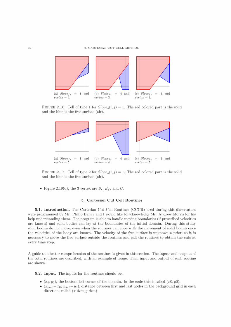
36 2. CARTESIAN CUT CELL METHOD
(a) Slopefs = 1 andvertex = 4.
(b) Slopefs = 4 andvertex = 3.
(c) Slopefs = 4 andvertex = 4.
Figure 2.16. Cell of type 1 for Slopes(i, j) = 1. The red colored part is the solidand the blue is the free surface (air).
(a) Slopefs = 1 andvertex = 5.
(b) Slopefs = 4 andvertex = 4.
(c) Slopefs = 4 andvertex = 5.
Figure 2.17. Cell of type 2 for Slopes(i, j) = 1. The red colored part is the solidand the blue is the free surface (air).
∙ Figure 2.19(d), the 3 vertex are Ss, Efs and C.
5. Cartesian Cut Cell Routines
5.1. Introduction. The Cartesian Cut Cell Routines (CCCR) used during this dissertationwere programmed by Mr. Philip Bailey and I would like to acknowledge Mr. Andrew Morris for hishelp understanding them. The program is able to handle moving boundaries (if prescribed velocitiesare known) and solid bodies can lay at the boundaries of the initial domain. During this studysolid bodies do not move, even when the routines can cope with the movement of solid bodies oncethe velocities of the body are known. The velocity of the free surface is unknown a priori so it isnecessary to move the free surface outside the routines and call the routines to obtain the cuts atevery time step.
A guide to a better comprehension of the routines is given in this section. The inputs and outputs ofthe total routines are described, with an example of usage. Then input and output of each routineare shown.
5.2. Input. The inputs for the routines should be,
∙ (x0, y0), the bottom left corner of the domain. In the code this is called (x0, y0).∙ (xend −x0, yend − y0), distance between first and last nodes in the background grid in each
direction, called (x dim, y dim).
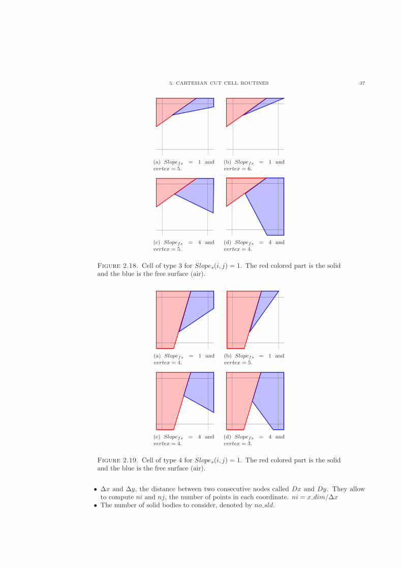
5. CARTESIAN CUT CELL ROUTINES 37
(a) Slopefs = 1 andvertex = 5.
(b) Slopefs = 1 andvertex = 6.
(c) Slopefs = 4 andvertex = 5.
(d) Slopefs = 4 andvertex = 4.
Figure 2.18. Cell of type 3 for Slopes(i, j) = 1. The red colored part is the solidand the blue is the free surface (air).
(a) Slopefs = 1 andvertex = 4.
(b) Slopefs = 1 andvertex = 5.
(c) Slopefs = 4 andvertex = 4.
(d) Slopefs = 4 andvertex = 3.
Figure 2.19. Cell of type 4 for Slopes(i, j) = 1. The red colored part is the solidand the blue is the free surface (air).
∙ Δx and Δy, the distance between two consecutive nodes called Dx and Dy. They allowto compute ni and nj, the number of points in each coordinate. ni = x dim/Δx
∙ The number of solid bodies to consider, denoted by no sld.
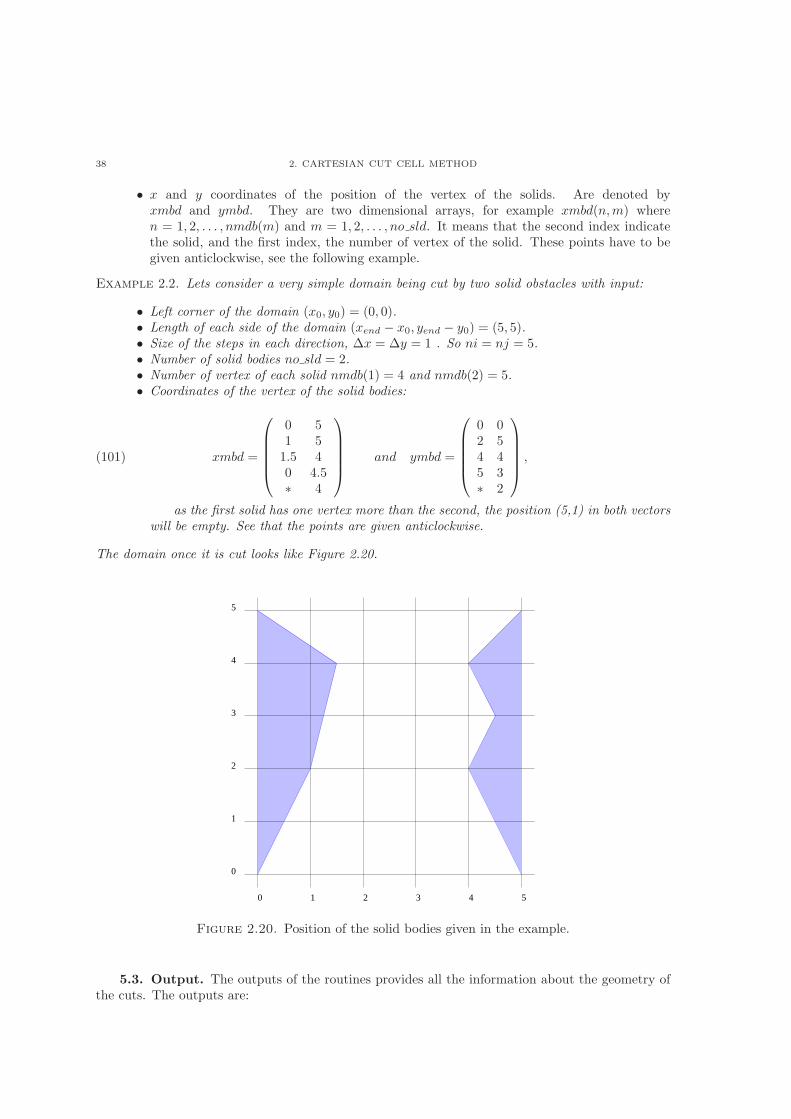
38 2. CARTESIAN CUT CELL METHOD
∙ x and y coordinates of the position of the vertex of the solids. Are denoted byxmbd and ymbd. They are two dimensional arrays, for example xmbd(n,m) wheren = 1, 2, . . . , nmdb(m) and m = 1, 2, . . . , no sld. It means that the second index indicatethe solid, and the first index, the number of vertex of the solid. These points have to begiven anticlockwise, see the following example.
Example 2.2. Lets consider a very simple domain being cut by two solid obstacles with input:
∙ Left corner of the domain (x0, y0) = (0, 0).∙ Length of each side of the domain (xend − x0, yend − y0) = (5, 5).∙ Size of the steps in each direction, Δx = Δy = 1 . So ni = nj = 5.∙ Number of solid bodies no sld = 2.∙ Number of vertex of each solid nmdb(1) = 4 and nmdb(2) = 5.∙ Coordinates of the vertex of the solid bodies:
xmbd =
⎛
⎜⎜⎜⎜⎝
0 51 51.5 40 4.5∗ 4
⎞
⎟⎟⎟⎟⎠
and ymbd =
⎛
⎜⎜⎜⎜⎝
0 02 54 45 3∗ 2
⎞
⎟⎟⎟⎟⎠
,(101)
as the first solid has one vertex more than the second, the position (5,1) in both vectorswill be empty. See that the points are given anticlockwise.
The domain once it is cut looks like Figure 2.20.
5
4
3
0
1
2
0 1 2 3 4 5
Figure 2.20. Position of the solid bodies given in the example.
5.3. Output. The outputs of the routines provides all the information about the geometry ofthe cuts. The outputs are:
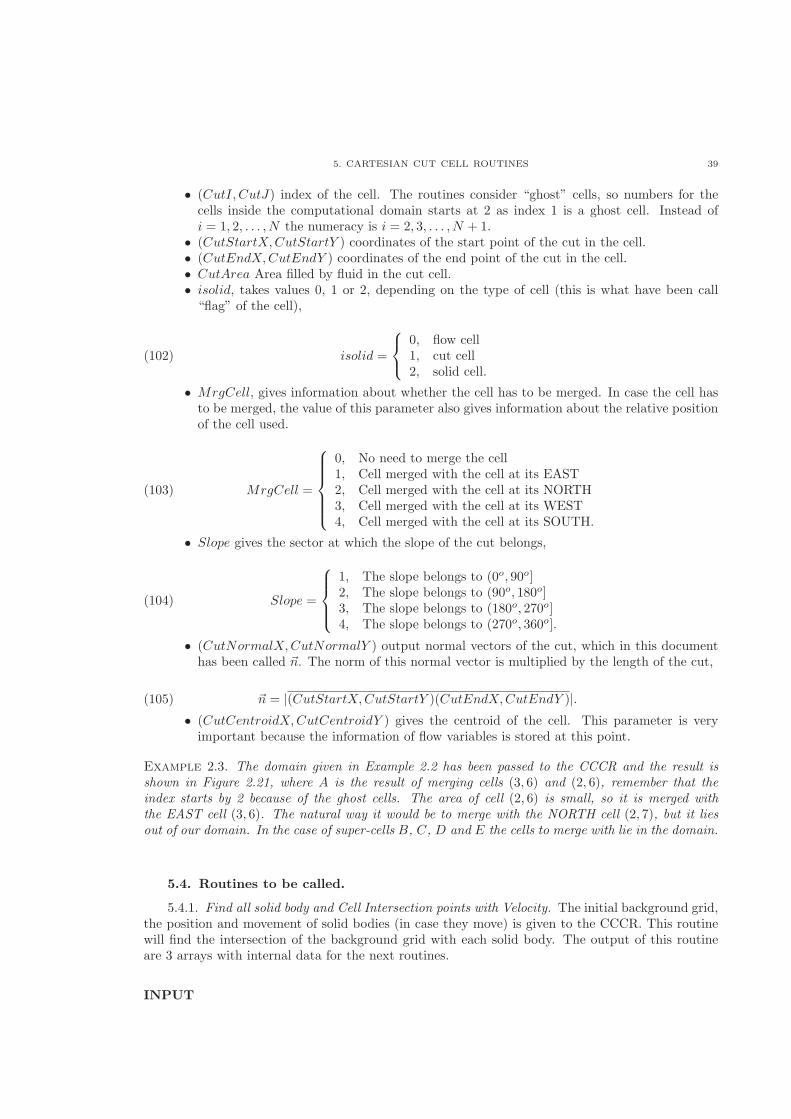
5. CARTESIAN CUT CELL ROUTINES 39
∙ (CutI, CutJ) index of the cell. The routines consider “ghost” cells, so numbers for thecells inside the computational domain starts at 2 as index 1 is a ghost cell. Instead ofi = 1, 2, . . . , N the numeracy is i = 2, 3, . . . , N + 1.
∙ (CutStartX,CutStartY ) coordinates of the start point of the cut in the cell.∙ (CutEndX,CutEndY ) coordinates of the end point of the cut in the cell.∙ CutArea Area filled by fluid in the cut cell.∙ isolid, takes values 0, 1 or 2, depending on the type of cell (this is what have been call
“flag” of the cell),
isolid =
⎧
⎨
⎩
0, flow cell1, cut cell2, solid cell.
(102)
∙ MrgCell, gives information about whether the cell has to be merged. In case the cell hasto be merged, the value of this parameter also gives information about the relative positionof the cell used.
MrgCell =
⎧
⎨
⎩
0, No need to merge the cell1, Cell merged with the cell at its EAST2, Cell merged with the cell at its NORTH3, Cell merged with the cell at its WEST4, Cell merged with the cell at its SOUTH.
(103)
∙ Slope gives the sector at which the slope of the cut belongs,
Slope =
⎧
⎨
⎩
1, The slope belongs to (0o, 90o]2, The slope belongs to (90o, 180o]3, The slope belongs to (180o, 270o]4, The slope belongs to (270o, 360o].
(104)
∙ (CutNormalX,CutNormalY ) output normal vectors of the cut, which in this documenthas been called n. The norm of this normal vector is multiplied by the length of the cut,
n = ∣(CutStartX,CutStartY )(CutEndX,CutEndY )∣.(105)
∙ (CutCentroidX,CutCentroidY ) gives the centroid of the cell. This parameter is veryimportant because the information of flow variables is stored at this point.
Example 2.3. The domain given in Example 2.2 has been passed to the CCCR and the result isshown in Figure 2.21, where A is the result of merging cells (3, 6) and (2, 6), remember that theindex starts by 2 because of the ghost cells. The area of cell (2, 6) is small, so it is merged withthe EAST cell (3, 6). The natural way it would be to merge with the NORTH cell (2, 7), but it liesout of our domain. In the case of super-cells B, C, D and E the cells to merge with lie in the domain.
5.4. Routines to be called.
5.4.1. Find all solid body and Cell Intersection points with Velocity. The initial background grid,the position and movement of solid bodies (in case they move) is given to the CCCR. This routinewill find the intersection of the background grid with each solid body. The output of this routineare 3 arrays with internal data for the next routines.
INPUT
40 2. CARTESIAN CUT CELL METHOD
5
4
3
0
1
2
0 1 2 3 4 5
A
C
D
EB
Figure 2.21. Grid resultant of applying the CCCR to the geometry given. Mergedcells A, B, C, D and E.
∙ SBMaxNumberOfPnts, (Integer) maximum number of vertex in the solid bodies plus 1. Itmeans, in the case we have 5 triangles, 2 rectangle, one 7-sides-polygon and 3 pentagons,this value would be 8 because the maximum number of sides amount our polygons is 7,and the first vertex is repeat, one more is added, so this value is 8.
∙ NumberOfSlds, (Integer) Number of solid bodies in the domain.∙ SBXCoordinates, (Array) X vertex of the Solid bodies. It has as many indexes as solid
bodies (NumberOfSlds) to store the x-coordinates of the vertex in each index.∙ SBYCoordinates, (Array) Y vertex of the Solid bodies. It has as many index as solid bodies(NumberOfSlds) to store the y-coordinates of the vertex in each index.
∙ SBUVel, (Array) U velocity of each vertex of the solid bodies.∙ SBVVel, (Array) V velocity of each vertex of the solid bodies.∙ SBNumberOfPnts, (Array) gives the number of vertex (or sides) plus one of each solid
body. In the case of just one solid body it is equal to SBMaxNumberOfPnts∙ DeltaX, DeltaY, (Reals) distance between two consecutive nodes in the background gridin each direction.
∙ CompDomainStartX, (Real) X-coordinate of the starting point of our domain, usually isset to 0.
∙ CompDomainStartY, (Real) Y-coordinate of the starting point of our domain, usually isset to 0.
∙ XLength, Length of the domain in the X-direction.∙ YLength, Length of the domain in the X-direction.
INPUT & OUTPUT
∙ MrgCellLst, (Array) List of Merged cells.∙ AllSldBdysIsectPntLst, (Array) List of all the intersection points (with the solid bodies).∙ SBNumberOfIsectPnts, (Array) Number of intersection points for each solid body.
5. CARTESIAN CUT CELL ROUTINES 41
5.4.2. Find all Isolid data. Isolid is an array that has to be initializated to zero before call thesubroutine. This routine will assign an isolid value (0 for Flow, 1 foe Cut and 2 for Solid cells) toeach cell of the background domain.
INPUT
∙ NumberOfSlds, (Integer) Number of solid bodies in the domain.∙ DeltaX, DeltaY, (Reals) distance between two consecutive nodes in the background gridin each direction.
∙ CompDomainStartX, (Real) X-coordinate of the starting point of our domain,usually isset to 0.
∙ CompDomainStartY, (Real) Y-coordinate of the starting point of our domain, usually isset to 0.
∙ XLength, Length of the domain in the X-direction.∙ YLength, Length of the domain in the X-direction.∙ AllSldBdysIsectPntLst, (Array) List of all the intersection (with the solid bodies) points.
Output of the previous subroutine.∙ SBNumberOfIsectPnts, (Array) Number of Intersection points for each solid body. Outputof the previous subroutine.
INPUT & OUTPUT
∙ Isolid, Array that describes the relative position of each cell with respect to the domain.It means, it has value 0 for a flow cell, 1 for a cut cell and 2 for a solid cell. It is 2 cellswider and longer because of the ghost cells.
5.4.3. Get Next Cut From All Isolid List. This routine go through each point computing thegeometrical details of Cut cells. This subroutine should be called for every solid body in the domain.
INPUT
∙ AllSldBdysIsectPntLst, (Array) List of all the intersection points (with the solid bodies).Output of the first subroutine.
∙ NumberOfIsectPnts, (Array) Number of intersection points for the selected solid body. Isone of the values in the array NumberOfIsectPnts that is Output of the first subroutine.
∙ RequiredSBIndex, Index of the body that we want to study.
OUTPUT
∙ CutStartX, (Real) X-coordinate of the first cut.∙ CutStartY, (Real) Y-coordinate of the first cut.∙ CutEndX, (Real) X-coordinate of the last cut.∙ CutEndY, (Real) Y-coordinate of the last cut.∙ CutI, (Integer) X-direction index of the cut.∙ CutJ, (Integer) Y-direction index of the cut.∙ CutNormalX, (Real) X-component of the normal vector of the cut.∙ CutNormalY, (Real) Y-component of the normal vector of the cut.∙ CutU, (Real) U component of the velocity of the cut.∙ CutV, (Real) V component of the velocity of the cut.∙ CutArea, (Real) Area of the cut cell.∙ CutCentroidX, (Real) X-coordinate of the centre point of the cut cell.∙ CutCentroidY, (Real) X-coordinate of the centre point of the cut cell.
42 2. CARTESIAN CUT CELL METHOD
∙ MrgCell, (Integer) variable saying whether the cell needs to be merged, and the relativeposition of the cell to merge with.
∙ Slope, (Real) Gives the slope (angle) of the cut.
INPUT & OUTPUT
∙ NextIsectPnt (Real) next intersection point.∙ IsectPntIndex (Integer) index of the next intersection point in the intersection point list.
CHAPTER 3
Numerical Method
1. Introduction
The technique (CCCM and Godunov’s type Method) use in this dissertation has been successfullyused by the CMMFA for the SWE [24, 25, 60, 61, 100, 140, 161, 166]. It also has been applied to theEE and NSE in two fluids systems [63, 117, 118, 119]. The CMMFA is responsible for the softwareAMAZON-CC, based on the SWE, and AMAZON-SC, based on the NSE for two fluid systems.LeVeque uses also this technique in [77, 78] and also produced the CLAWPACK software. DamFlowis also a software about SWE done by University of Malaga [23]. Toro in his [148] gives details ofthe employed method for both systems of equations.
The ACM [30] is used to obtain the solution of the incompressible NSE. Applying a perturbation tothe conservation of mass equation on a fictitious time a new set of equations are obtained. This per-turbation makes the system compressible in fictitious time. The solutions of the perturbed system(compressible) converges in fictitious time to the solutions of the incompressible NSE. The new setof equations are an hyperbolic system of equations which is solved using a cell-centred finite volumeapproach. A high order Godunov type upwind scheme is used where information is stored at cellcentres. For each time iteration values are linearly reconstructed at each side of cell interface usingslope limiters to avoid under/over oscillations. A local RP is set at each cell interfaces using thereconstructed values. A quick and robust Riemann Solver (RS) is required as the exact Riemannsolution is computer expensive.
These techniques are applied to a two dimensional incompressible one fluid system. The density �is assumed to be constant, these are the parameters used in the equation,
∙ u, v velocities in the x and y direction respectively, V = (u, v),∙ p dynamic pressure,
∙ g gravity acceleration, that would be included in vector B,∙ � denotes the viscosity.
Using this notation, incompressible NSE (EE � = 0) equations are written as follows,
∙ Conservation of mass,
∇ ⋅ V = 0(106)
∙ Conservation of momentum,
∂V
∂t+∇ ⋅
(
V × V − T)
= B(107)
43
44 3. NUMERICAL METHOD
being T = −Ip for the EE and T = �∇ ⋅ V − Ip, with � the dynamic viscosity, for theNSE.
∙ Incompressibility constraint,
∇ ⋅ V = 0(108)
In this case the conservation of mass (106) and the incompressibility constraint (108) are the samebecause density is constant. The ACM will be introduced and applied for the presented case in nextsection.
2. Artificial Compressibility Method
The Artificial Compressibility Method (ACM) was first developed by Alexander Joel Chorin in 1967and has been reprinted by the AIAA Selected Reprint Series (1968), Physical Society of Japan (1971)and Journal of Computational Physics (1997) [30]. In 2000, Professor Chorin received the NorbertWiener Prize in Applied Mathematics for his contribution to Fluid Dynamics and also holds theUniversity of California Professor award.
The ACM was initially developed to solve steady problems while unsteady problems would be solvedusing the Projection Method also by Chorin [31]. In fact, using Chorin’s words about the ProjectionMethod “Essentially it constitutes an extension to time dependent problems of the artificial com-pressibility method introduced in [30] for steady flow problems” [31]. The ACM has been applied tounsteady problems by many authors. Rogers and D. Kwak [128, 129] used the ACM for the un-steady case but they already open the possibility to use it directly in the unsteady cases “Althoughthe current study is limited to steady-state problems, it is shown that this entire formulation can beused for solving unsteady problems” [129]. Since then the ACM has been successfully applied for thesimulation of incompressible flow in different flow system (one/two fluids) and the considered mesh(structured/unstructured).
In the ACM a new fictitious time scale (pseudo time �) is defined between two consecutive timesteps. The relation between (physical) time t and pseudo time � is given by Kelecy and Pletcherin [71] “The solution at a given physical time level is approached asymptotically as a steady statesolution in pseudo-time”. A tolerance value tol is defined, the system is iterated in pseudo time(index m) until the difference in two consecutive pseudo time steps is below this tolerance. Thevalue obtained in the last pseudo iteration of time n is considered the value at next time step n+ 1and the start value for the iteration in pseudo time.
The incompressibility constraint/conservation of mass (106/108) is perturbed adding a derivative ofpressure in pseudo time obtaining,
1
�
∂p
∂�+∇ ⋅ V = 0,(109)
where � is a constant (units of pressure) and � is the pseudo-time. For simplicity this equationis multiplied by � so equations (110) and (111) are the set of equations in Chapter 6 were called“pseudo-compressible NSE”:
2. ARTIFICIAL COMPRESSIBILITY METHOD 45
∂p
∂�+ �∇ ⋅ V = 0,(110)
∂V
∂t+∇ ⋅
(
V × V − T)
= B,(111)
where,
(112) V =
[uv
]
, F =
[V u+ pi
V v + pj
]
and B =
[Bx
By
]
=
[00
]
.
2.1. Artificial Compressibility Parameter. There is uncertainty in the literature about theappropriate value of the artificial compressibility parameter, �. Peric in [39] says “Typical valuesof � used in various methods based on artificial compressibility were in the range between 0.1 and10”. Bet et al. [17] apply � values between 0.4 and 2.0 for the case they study. They also plot aconvergence rate for different � values. Lee at al. [76], used a range of � values between 0.5 and 10,finding � = 1 when the “most acceptable convergence” is obtained. Li et al. [81] used an artificialcompressibility parameter � the ℓ2 norm of the velocity multiplied by a constant � which valuesbelongs to the interval [3, 10]. Qian et al. [117, 118, 119] used similar � values understanding theywork with a two phase flow, and they used �/�, where � is the density to modify the conservationof mass equation. “It was found that a � value between 200 and 2000 produced good results for thecurrent test cases” [119], the value density used in water was � = 1000, so �/� takes values between0.2 and 2, while in air � = 1 therefore � was between 200 and 2000. In Experiments a value of� = 0.01 has been successfully applied for the lid-driven Cavity flow and for the lid-driven Couetteflow.
Malan et al. [94] do not use a constant value of the artificial parameter � through the whole com-putation. Instead � is recomputed automatically at every time step, computing convective anddiffusive values for � and using the maximum of them. A comparison of results using constant orautomatically recomputed � values is presented in [93].
Nithiarasu [107] gives a methodology in which it is possible to find an appropriate value (constantthrough the computation) for � and Δt. In Nithiarasu’s computation of � the convective velocity,vconv and the diffusive velocity, vdiff , are required and defined as,
(113) vconv =√uu and vdiff =
2
ℎRe,
where u is the maximum value of the velocity in the domain, and ℎ the grid size. The appropriatevalue for the artificial compressibility parameter is given by
(114) � = max(�, vconv, vdiff ),
where � is a constant value which in Nithiarasu’s work has the value 0.5. Similarly for the timeinterval, Δt, Nithiarasu computed a convective time Δtconv and a diffusive time Δtdiff ,
46 3. NUMERICAL METHOD
(115) Δtconv =ℎ
vconv + �and Δtdiff =
ℎ2Re
2,
and consider the value for Δt as:
Δt = �Δtmin(Δtconv,Δtdiff ),(116)
where �Δt is a safety value varying in the interval (0.5, 2). A different value is given in [119]: “thetime step Δt used for advancing the solution was within the range 5× 10⁻⁵ - 5× 10⁻⁴ s”.
In this work different values of � and Δt has been applied which will be more explained in followingChapters (5, 6 and 7)
3. Godunov’s Method
Godunov’s most influential work is in the area of applied and numerical mathematics has had amajor impact on science and engineering, particularly in the development of methodologies used inComputational Fluid Dynamics (CFD). Godunov’s theorem: All linear monotone scheme for theconvection equation are necessarily first order accurate (see proof in [57]).
On 1-2 May, 1997 a symposium entitled: Godunov-Type Numerical Methods, was held at the Uni-versity of Michigan to honour Godunov. These methods are widely used to compute continuumprocesses dominated by wave propagation. On the following day, 3rd May, Godunov received anhonorary degree from the University of Michigan.
Godunov’s scheme is a conservative numerical scheme for solving PDE. In this method, the conserva-tive variables are considered as piecewise constant over the mesh cells at each time step and the timeevolution is determined by the exact solution of the RP (shock tube)at the inter-cell boundaries [57].
Guinot in [51] explained the potential of this method: “As mentioned in previous chapters and asillustrated by a number of authors on simple examples (see e.g. LeVeque [77] or Toro [148]), globallynon-conservative numerical methods lead to errors in the computation of both the amplitude and/orcelerity of shocks... This is because several initial conditions may lead to the same final state whenthe flow is discontinuous. For this reason Godunov sought a conservative alternative to the Method ofCharacteristics to solve systems of conservation laws... Although being only first-order accurate, andtherefore leading to considerable smearing of waves and discontinuities, the scheme allowed shocksto be represented correctly, both in terms of celerity and amplitude”.
Van Leer gives a possible definition of Godunov-type methods in [151]: “If we define Godunov-typemethods as non-oscillatory finite volume schemes that incorporate the solution (exact or approxi-mate) to Riemann initial-value problem, or a generalization of it”.
The original Godonov’s method consists of three different steps:
(1) Define a piece-wise constant distribution of data in the domain. At each cell the averagevalue is computed:
3. GODUNOV’S METHOD 47
Un(i,j) =
1
Ω(i,j)
∫
(i,j)
U(x, y; tn)dΩ(i,j),(117)
all the points in cell (i, j) will have the value of the computed average
U(x, y; tn) = Un(i,j), if (x, y) ∈ Ω(i, j).(118)
(2) At each cell interface, e.g. (i+1/2,j), solve the local RP for the conservation laws using the
averaged constant states at each side of the interface, denoted Fn(i+1/2,j).
(3) Update the value at each cell using the solution of the RP:
Un+1i,j = Un
i,j +∑
l∈∂Ω(i,j)
Fnl .(119)
A restriction in time is enforced to avoid wave iteration within cells, i.e. more thanone wave travelling through each cell,
Δt ≤12 min(Δx,Δy)
Snmax
,(120)
where Snmax denotes the maximum wave velocity at time tn in the entire domain.
3.1. Improvement to step (1): In this work a similar methodology is applied with someimprovements. Instead of considering piecewise constant values at cells, a linear reconstructionwithin cells is used, so a piecewise linear function is obtained. Slope limiters are used to avoidspurious over and undershoots. A description of the reconstruction applied is given in Section 4.2[51, 57, 78, 148].
3.2. Improvement to step (2): The methodology implies the solution of local RP at everycell interface at every time. An efficient solver is required and will be explained in Section 5.
3.3. Application of step (3) and the ACM:. Using the same notation for the velocity,pressure and flux given in equation (112) and using the subscripts ⋅(i,j) to indicate average values incell (i, j) stored at cell centres, an implicit scheme in real time is used here for equation (111). Thereal time level is denoted by n.
(121)Ω(i,j)
Δt
(
V n+1(i,j) − V n
(i,j)
)
+
⎛
⎝∑
l∈∂Ω(i,j)
(FS)l −BΩ
⎞
⎠
n+1
= 0.
For equation (110) an implicit scheme in pseudo-time is used and the pseudo-time level is denotedby m,
Ω(i,j)
Δ�
(
pm+1(i,j) − pm(i,j)
)
+
⎛
⎝∑
l∈∂Ω(i,j)
(V S)l
⎞
⎠
m+1
= 0.(122)
The quantities at pseudo-time step m + 1 approaches the solution at next time step n + 1 in thelimit as m→ ∞. As the solutions of the pseudo-incompressible NSE converges in fictitious time to
48 3. NUMERICAL METHOD
the solutions of the incompressible NSE: “it is possible to change in equation (121) the index n+ 1by the index m+ 1 obtaining” [71],
(123)Ω(i,j)
Δt
(
V m+1(i,j) − V n
(i,j)
)
+
⎛
⎝∑
l∈∂Ω(i,j)
(FS)l −BΩ
⎞
⎠
m+1
= 0.
Now it is possible to merge equations (122) and (123) in the following equation,
(124)Ω(i,j)
Δ�(I − I0)∂U(i,j) +
Ω(i,j)
ΔtI0(∂U(i,j) +Um
(i,j) −Un(i,j))
+
⎛
⎝∑
l∈∂Ω(i,j)
(FS)l −BΩ(i,j)
⎞
⎠
m+1
= 0,
where ∂U(i,j) = Um+1(i,j) −Um
(i,j), I = diag(1, 1, 1), I0 = diag(1, 1, 0) and
U =
⎡
⎣
uvp
⎤
⎦ , F =
⎡
⎣
V u+ pi
V v + pj
�V
⎤
⎦ and B =
⎡
⎣
Bx
By
0
⎤
⎦ .(125)
4. Flux Calculation
The flux function F is divided into inviscid flux FI and viscous flux FV (� = 1/Re). Each one ofthese is projected into the x and y directions giving four 1-dimensional fluxes,
(126) F = FI +1
ReFV = Fx
I + FyI +
1
Re(Fx
V + FyV )
=
⎡
⎣
u2 + puv�u
⎤
⎦+
⎡
⎣
uvv2 + p�v
⎤
⎦+1
Re
⎛
⎝
⎡
⎣
uxvx0
⎤
⎦+
⎡
⎣
uyvy0
⎤
⎦
⎞
⎠ .
For the viscous flux, a central difference scheme is applied to compute the derivatives in FxV and
FyV [118]. In the computation of the inviscid flow, FI , second order accuracy is achieved using the
procedure explained below.
4.1. Viscous flux. The viscous fluxes are written as,
FxV Sx =
⎡
⎣
�uxSx
�vxSx
0
⎤
⎦ and F xV Sy =
⎡
⎣
�uySy
�vySy
0
⎤
⎦ .(127)
A central difference scheme is applied for the computation of the viscous flux, [118]. Defining matrixC as follows,
4. FLUX CALCULATION 49
C =
⎡
⎣
� 0 00 � 00 0 0
⎤
⎦ ,(128)
it is possible to write FxV as a function of vectors U(⋅,⋅),
(129) (FxV Sx)
mi+ 1
2=
⎡
⎣
�(umi+1,j − umi,j)Sx∣i+ 12/Δx
�(vmi+1,j − vmi,j)Sx∣i+ 12/Δx
0
⎤
⎦ =
C
Δx
(
Umi+1,jSx∣i+ 1
2−Um
i,jSx∣i+ 12
)
,
and FxV as function of vectors U(⋅,⋅),
(130) (FxV Sx)i− 1
2=
⎡
⎣
�(umi,j − umi−1,j)Sx∣i− 12/Δx
�(vmi,j − vmi−1,j)Sx∣i− 12/Δx
0
⎤
⎦ =
C
Δx
(
Umi,jSx∣i− 1
2−Um
i−1,jSx∣i− 12
)
.
The viscosity fluxes at cell (i, j) ,FxV , are written as a function of U(i+1,j), U(i,j) and U(i−1,j). In
the same way in the y–direction FyV can be written as a function of U(i,j+1), U(i,j) and U(i,j−1).
4.2. Inviscid Flux. Reconstruction. To compute the inviscid flux values of the flow vari-ables, velocity and pressure, are required at cell interfaces. The technique applied stores these valuesonly at cell centres, and values at cell interfaces have to be reconstructed every time step. In the caseof flow cells this reconstruction is straight forward as all the distances are known, but in the case ofcut cells distances are unknown a priori. Also one of the interfaces of cut cells is a fluid/solid inter-face for solid body and fluid/air interface for free surface, so different boundary conditions and/orfree surface conditions have to be applied on them.
At fluid/solid(air) interfaces the values of velocities and pressure are only known at one side of theinterface. To impose values at the interface the ghost cell technique is applied where a point R isdefined as mirror point of the centre of the cut cell. The values at the ghost cell R are given usinginformation from the fluid depending on the interface presented (fluid/solid or fluid/air). Compu-tation of the ghost point R is described in next section and the values on it are described in Section7 for solid body and in Section 5 for free surface.
Once the distances between centroids and interfaces and the values at each side of the interface areknown, reconstruction can be computed. Using information of flow, cut and ghost surrounding cells,a gradient is computed within each cell. The value at each point of the cell is calculated using thevalue at centroid of cell, the distance between the point and the centroid, and the gradient in thecell. So these values for each side of the interface are computed. Once reconstructed values areobtained at each side of the cell interface, a RP is solved providing the value of the inviscid flux atthe cell interface.
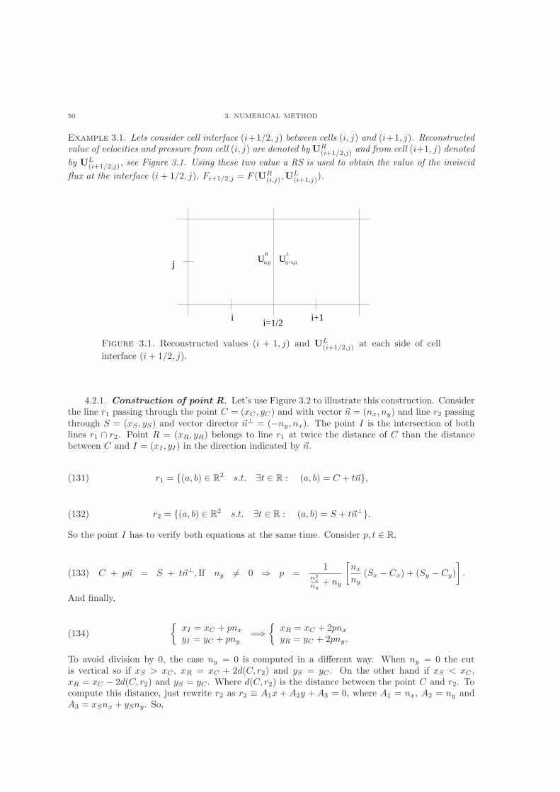
50 3. NUMERICAL METHOD
Example 3.1. Lets consider cell interface (i+1/2, j) between cells (i, j) and (i+1, j). Reconstructedvalue of velocities and pressure from cell (i, j) are denoted by UR
(i+1/2,j) and from cell (i+1, j) denoted
by UL(i+1/2,j), see Figure 3.1. Using these two value a RS is used to obtain the value of the inviscid
flux at the interface (i+ 1/2, j), Fi+1/2,j = F (UR(i,j),U
L(i+1,j)).
i=1/2
U U(i+1,j)
LR
(i,j)
i i+1
j
Figure 3.1. Reconstructed values (i + 1, j) and UL(i+1/2,j) at each side of cell
interface (i+ 1/2, j).
4.2.1. Construction of point R. Let’s use Figure 3.2 to illustrate this construction. Considerthe line r1 passing through the point C = (xC , yC) and with vector n = (nx, ny) and line r2 passingthrough S = (xS , yS) and vector director n⊥ = (−ny, nx). The point I is the intersection of bothlines r1 ∩ r2. Point R = (xR, yR) belongs to line r1 at twice the distance of C than the distancebetween C and I = (xI , yI) in the direction indicated by n.
r1 = {(a, b) ∈ ℝ2 s.t. ∃t ∈ ℝ : (a, b) = C + tn},(131)
r2 = {(a, b) ∈ ℝ2 s.t. ∃t ∈ ℝ : (a, b) = S + tn⊥}.(132)
So the point I has to verify both equations at the same time. Consider p, t ∈ ℝ,
(133) C + pn = S + tn⊥, If ny ∕= 0 ⇒ p =1
n2x
ny+ ny
[nxny
(Sx − Cx) + (Sy − Cy)
]
.
And finally,
{xI = xC + pnxyI = yC + pny
=⇒{xR = xC + 2pnxyR = yC + 2pny.
(134)
To avoid division by 0, the case ny = 0 is computed in a different way. When ny = 0 the cutis vertical so if xS > xC , xR = xC + 2d(C, r2) and yS = yC . On the other hand if xS < xC ,xR = xC − 2d(C, r2) and yS = yC . Where d(C, r2) is the distance between the point C and r2. Tocompute this distance, just rewrite r2 as r2 ≡ A1x + A2y + A3 = 0, where A1 = nx, A2 = ny andA3 = xSnx + ySny. So,
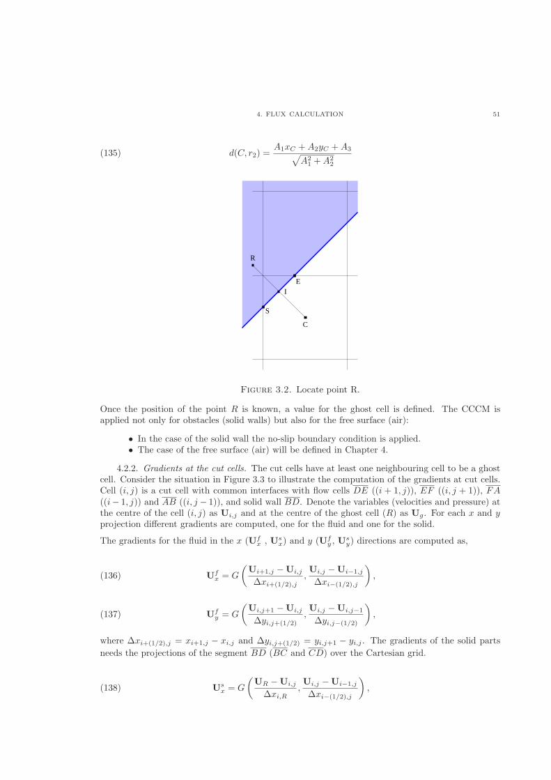
4. FLUX CALCULATION 51
d(C, r2) =A1xC +A2yC +A3
√
A21 +A2
2
(135)
S
EI
R
C
Figure 3.2. Locate point R.
Once the position of the point R is known, a value for the ghost cell is defined. The CCCM isapplied not only for obstacles (solid walls) but also for the free surface (air):
∙ In the case of the solid wall the no-slip boundary condition is applied.∙ The case of the free surface (air) will be defined in Chapter 4.
4.2.2. Gradients at the cut cells. The cut cells have at least one neighbouring cell to be a ghostcell. Consider the situation in Figure 3.3 to illustrate the computation of the gradients at cut cells.Cell (i, j) is a cut cell with common interfaces with flow cells DE ((i + 1, j)), EF ((i, j + 1)), FA((i− 1, j)) and AB ((i, j − 1)), and solid wall BD. Denote the variables (velocities and pressure) atthe centre of the cell (i, j) as Ui,j and at the centre of the ghost cell (R) as Ug. For each x and yprojection different gradients are computed, one for the fluid and one for the solid.
The gradients for the fluid in the x (Ufx , Us
x) and y (Ufy , U
sy) directions are computed as,
Ufx = G
(Ui+1,j −Ui,j
Δxi+(1/2),j,Ui,j −Ui−1,j
Δxi−(1/2),j
)
,(136)
Ufy = G
(Ui,j+1 −Ui,j
Δyi,j+(1/2),Ui,j −Ui,j−1
Δyi,j−(1/2)
)
,(137)
where Δxi+(1/2),j = xi+1,j − xi,j and Δyi,j+(1/2) = yi,j+1 − yi,j . The gradients of the solid parts
needs the projections of the segment BD (BC and CD) over the Cartesian grid.
Usx = G
(UR −Ui,j
Δxi,R,Ui,j −Ui−1,j
Δxi−(1/2),j
)
,(138)
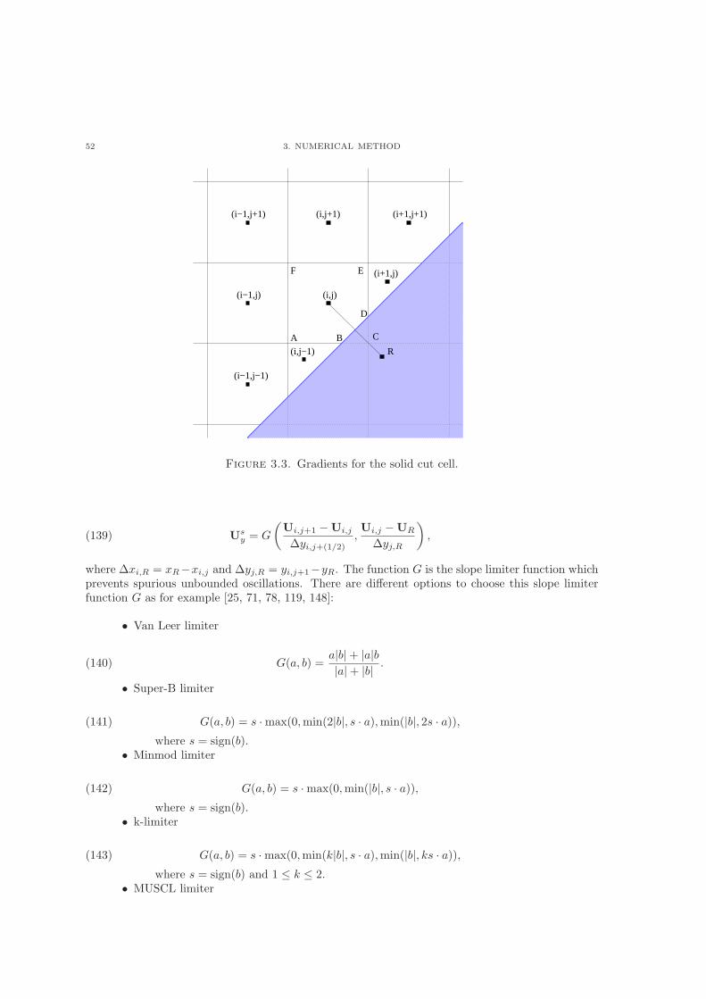
52 3. NUMERICAL METHOD
(i−1,j−1)
(i,j−1)
(i,j)
(i+1,j+1)(i−1,j+1)
(i+1,j)E
R
A
F
D
B C
(i−1,j)
(i,j+1)
Figure 3.3. Gradients for the solid cut cell.
Usy = G
(Ui,j+1 −Ui,j
Δyi,j+(1/2),Ui,j −UR
Δyj,R
)
,(139)
where Δxi,R = xR−xi,j and Δyj,R = yi,j+1−yR. The function G is the slope limiter function whichprevents spurious unbounded oscillations. There are different options to choose this slope limiterfunction G as for example [25, 71, 78, 119, 148]:
∙ Van Leer limiter
G(a, b) =a∣b∣+ ∣a∣b∣a∣+ ∣b∣ .(140)
∙ Super-B limiter
G(a, b) = s ⋅max(0,min(2∣b∣, s ⋅ a),min(∣b∣, 2s ⋅ a)),(141)
where s = sign(b).∙ Minmod limiter
G(a, b) = s ⋅max(0,min(∣b∣, s ⋅ a)),(142)
where s = sign(b).∙ k-limiter
G(a, b) = s ⋅max(0,min(k∣b∣, s ⋅ a),min(∣b∣, ks ⋅ a)),(143)
where s = sign(b) and 1 ≤ k ≤ 2.∙ MUSCL limiter
5. THE RIEMANN PROBLEM 53
G(a, b) = s ⋅max
(
0,min
(
2, 2∣b∣, ∣a∣+ ∣b∣2
))
,(144)
where s = sign(b).
During this work the Van Leer limiter has been used. Once the flow and solid gradients in eachdirection are computed, a weighted average is done to obtain the total gradient in each direction(Ux
i,j , Uyi,j):
Uxi,j =
ΔysUsx +ΔyfU
fx
Δys +Δyfand Uy
i,j =ΔxsU
sy +ΔxfU
fy
Δxs +Δxf,(145)
where Δxf = ∣AB∣, Δxs = ∣BC∣, Δys = ∣CD∣ and Δyf = ∣DE∣. For flow cells, Δxs = Δys = 0, soUx = Uf
x and Uy = Ufy . Once the total gradients in cell (i, j) are computed they can be written in
vectorial form ( ∇U) as:
∇U =
[Ux
Uy
]
,(146)
so the value of U at every point (x, y) inside cell (i, j) has been reconstructed and can be writtenas,
U(x, y) = Ui,j + r ⋅ ∇U,(147)
where r is the normal distance vector from the centre of the cell (i, j) to the point (x, y).
5. The Riemann Problem
The Riemann Problem (RP) is a PDE that has the form [148],
Ut + F(U)x = 0,(148)
where the initial condition is piecewise continuous with a jump at one point, for example at x = 0,
U = U0(x) =
{UL if x ≤ 0,UR if x > 0.
(149)
Thanks to the ACM the pseudo-compressible NSE, (110, 111) are hyperbolic systems, all threeeigenvalues of the flux F (in fact of the linearized system using the Jacobian A = ∂F/∂U, seeSection 5.3) are real and distinct, so their eigenvectors are linearly independent. The solution of theRP contains three jump discontinuities dividing the solution space in four sectors as in Figure 5.
Definition 3.2. Characteristics or characteristics curves are curves x = x(t) in the x − t planealong which the PDE becomes an ODE (Ordinary Differential Equation) [148].
Example 3.3. Lets use this example to understand the previous definition. Consider the following1-D PDE:
ut + aux = 0, −∞ < x <∞, t > 0,(150)
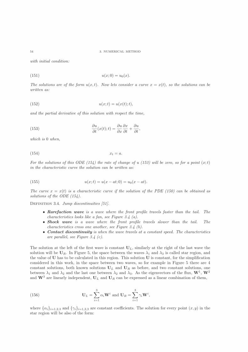
54 3. NUMERICAL METHOD
with initial condition:
u(x; 0) = u0(x).(151)
The solutions are of the form u(x, t). Now lets consider a curve x = x(t), so the solutions can bewritten as:
u(x; t) = u(x(t); t),(152)
and the partial derivative of this solution with respect the time,
∂u
∂t(x(t); t) =
∂u
∂x
∂x
∂t+∂u
∂t,(153)
which is 0 when,
xt = a.(154)
For the solutions of this ODE (154) the rate of change of u (153) will be zero, so for a point (x; t)in the characteristic curve the solution can be written as:
u(x; t) = u(x− at; 0) = u0(x− at).(155)
The curve x = x(t) is a characteristic curve if the solution of the PDE (150) can be obtained assolutions of the ODE (154).
Definition 3.4. Jump discontinuities [51].
∙ Rarefaction wave is a wave where the front profile travels faster than the tail. Thecharacteristics looks like a fan, see Figure 3.4 (a).
∙ Shock wave is a wave where the front profile travels slower than the tail. Thecharacteristics cross one another, see Figure 3.4 (b).
∙ Contact discontinuity is when the wave travels at a constant speed. The characteristicsare parallel, see Figure 3.4 (c).
The solution at the left of the first wave is constant UL, similarly at the right of the last wave thesolution will be UR. In Figure 5, the space between the waves �1 and �3 is called star region, andthe value of U has to be calculated in this region. This solution U is constant, for the simplificationconsidered in this work, in the space between two waves, so for example in Figure 5 there are 4constant solutions, both known solutions UL and UR as before, and two constant solutions, onebetween �1 and �2 and the last one between �2 and �3. As the eigenvectors of the flux, W1, W2
and W3 are linearly independent, UL and UR can be expressed as a linear combination of them,
UL =
3∑
i=1
�iWi and UR =
3∑
i=1
iWi,(156)
where {�i}i=1,2,3 and { i}i=1,2,3 are constant coefficients. The solution for every point (x, y) in thestar region will be also of the form:
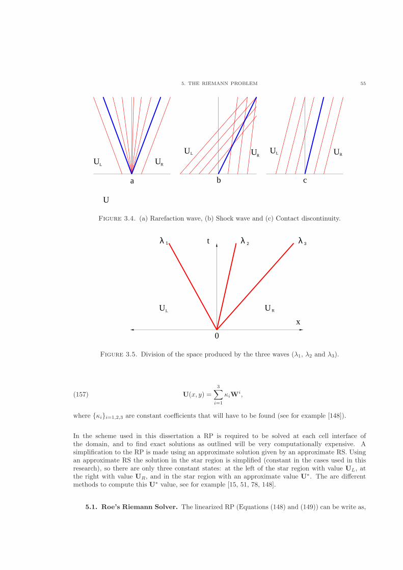
5. THE RIEMANN PROBLEM 55
L
UUU U
R
RL
L
a b c
U
U
UR
Figure 3.4. (a) Rarefaction wave, (b) Shock wave and (c) Contact discontinuity.
t
U
λ
U
λ
L R
32λ 1
0
x
Figure 3.5. Division of the space produced by the three waves (�1, �2 and �3).
U(x, y) =3∑
i=1
�iWi,(157)
where {�i}i=1,2,3 are constant coefficients that will have to be found (see for example [148]).
In the scheme used in this dissertation a RP is required to be solved at each cell interface ofthe domain, and to find exact solutions as outlined will be very computationally expensive. Asimplification to the RP is made using an approximate solution given by an approximate RS. Usingan approximate RS the solution in the star region is simplified (constant in the cases used in thisresearch), so there are only three constant states: at the left of the star region with value UL, atthe right with value UR, and in the star region with an approximate value U∗. The are differentmethods to compute this U∗ value, see for example [15, 51, 78, 148].
5.1. Roe’s Riemann Solver. The linearized RP (Equations (148) and (149)) can be write as,
56 3. NUMERICAL METHOD
∂U
∂t+A
∂U
∂x= 0,(158)
where A = ∂F/∂U which usually is not constant. Roe’s approach [127], consists of replacing matrix
A by a constant matrix A which is a function of the left and right states of the RP, A = A(UL, UR).
∂U
∂t+ A
∂U
∂x= 0.(159)
To be a reasonable approximation of the solution of equations (148 and 149), the matrix A shouldsatisfy the following conditions:
(1) A should have m real eigenvalues ( system (159) must be hyperbolic),
(2) A(UL, UR) → A when ∣UL − UR∣ → 0 (A(U,U) = A(U)),(3) conservation is satisfied, i.e. for any pair (U1, U2), the jump ΔF = F (U1) − F (U2) in the
flux is related to ΔU = U1 − U2 via the Rankine-Hugoniot condition,
ΔF = F (U1)− F (U2) = AU1 − AU2 = AΔU.(160)
Details about the construction of this solver can be found in [51].
A matrix A which satisfies the previous conditions is the matrix A evaluated at averaged values ofthe states from each side, U [71], where,
U =
⎡
⎣
uv
P
⎤
⎦ =1
2
⎡
⎣
(uL + uR)(vL + vR)(pL + pR)
⎤
⎦ .(161)
Denoting by R the matrix whose columns are the right eigenvectors of A and by Λ the diagonalmatrix consisting of the absolute values of the eigenvalues of A, the flux using Roe’s Riemannapproximation at the star region, denoted by FRoe, can be written as,
FRoe =1
2[FR + FL −D(UR − UL)] ,(162)
where D = RΛ ˜R−1 [117].
5.2. HLL Riemann Solver. The name is taken from the initials of Harten, Lax and Van Leer[53]. The idea is to compute the wave speeds SL and SR at which infinitely thin waves separatethe star region from the left and right states. The value at the star region is obtained using theRankine-Hugoniot condition (160) to both waves.
Different methods to compute the wave speeds SL and SR can be found for example in [51, 78, 148].The values for the wave speeds used in this dissertation are:
SL = min(uL − cL, uR − cR); SR = max(uL + cL, uR + cR).(163)
5. THE RIEMANN PROBLEM 57
The value of F in the star region denoted by FHLL can be written as (see details in [15, 51, 148]),
FHLL = t1FR + t2FL − t3(UR −UL),(164)
where
t1 =min(SR, 0)−min(0, SL)
SR − SL, t2 = 1− t1, and t3 =
SR∣SL∣ − SL∣SR∣2(SR − SL)
.(165)
5.3. Matrix A. The RP is linearized using the Jacobian matrix of function F. This matrix iscomputed as,
A =∂F
∂U=
⎡
⎣
2unx + vny uny nxvnx unx + 2vny ny�nx �ny 0
⎤
⎦(166)
The RP solved in this work are always 1-D, and the flux function F is split in the x and y directionsobtaining,
Fx =
⎡
⎣
u2 + �puvu
⎤
⎦ and Fy =
⎡
⎣
uvv2 + �p
v
⎤
⎦(167)
Matrix A will also be split in each direction, Ax and Ay ,
Ax =∂Fx
∂U=
⎡
⎣
2u 0 1v u 0� 0 0
⎤
⎦ ; Ay =∂Fy
∂U=
⎡
⎣
v u 00 2v 10 � 0
⎤
⎦ .(168)
For the Roe’s RS the matrix D which is the multiplication of matrices R (the columns being theright eigenvectors of A), Λ (absolute values of the eigenvalues of A in the main diagonal) and L (therows being the left eigenvectors of A) are also needed for each direction. Defining
cx =√
u2 + � cy =√
v2 + �,(169)
the diagonal matrices with the absolute values of the eigenvalues of Ax and Ay are
(170) Λx =
⎡
⎣
∣u∣ 0 00 ∣u+ cx∣ 00 0 ∣u− cx∣
⎤
⎦ and Λy =
⎡
⎣
∣v∣ 0 00 ∣v + cy∣ 00 0 ∣v − cy∣
⎤
⎦ .
For simplicity the elements of the matrix Λ are going to be denoted by �xi , �yi with i = 1, 2, 3
depending on the direction. The right matrices Rx and Ry, with the right eigenvectors of Ax ascolumns are,
58 3. NUMERICAL METHOD
(171) Rx =
⎡
⎣
0 cx�2x cx�
3x
1 v�2x −v�3x0 cx cx
⎤
⎦ and Ry =
⎡
⎣
1 u�2y −u�3y0 cy�
2y cy�
3y
0 cy cy
⎤
⎦ ,
and the left matrices Lx and Ly with the left eigenvectors of Ax as rows are,
(172) Lx =1
c2
⎡
⎣
−uv c2x −v�1/2 0 −�3x/2−1/2 0 �2x/2
⎤
⎦ and Ly =1
c2
⎡
⎣
c2y −uv −u�0 1/2 −�3y/20 −1/2 �2y/2
⎤
⎦ .
Finally matrices Dx and Dy have the following form,
(173) Dx =
1
c2x
[(cx/2)(�2∣�2∣ − �3∣�3∣) 0 (cx�2�3/2)(∣�3∣ − ∣�2∣)
v(−∣�1∣u + (�2∣�2∣ + �3∣�3∣/2)) ∣�1∣c2x −(v�∣�1∣) − (v�2�3/2)(∣�2∣ + ∣�3∣)
(cx/2)(∣�2∣ − ∣�3∣) 0 (cx/2)(�2∣�3∣ − �3∣�2∣)
]
and
(174) Dy =
1
c2y
[∣�1∣c
2y u(−∣�1∣v + (�2∣�2∣ + �3∣�3∣/2)) −(u�∣�1∣) − (u�2�3/2)(∣�2∣ + ∣�3∣)
0 (cy/2)(�2∣�2∣ − �3∣�3∣) (cy�2�3/2)(∣�3∣ − ∣�2∣)0 (cy/2)(∣�2∣ − ∣�3∣) (cy/2)(�2∣�3∣ − �3∣�2∣)
]
.
6. Merged Cells Contributions
In Section 3 is explained how the CCCM deals with the merged cells, see Figure 2.11. Thecontributions of mass and momentum from the small cell A are transmitted to the bigger cell B.Consider the merged cell to be denoted as C and the area ΩC = ΩA + ΩB . The value of velocitiesand pressure at the centre of the merged cell C is the weighted average of the values of cells A andB,
UnC =
UnAΩA +Un
BΩB
ΩA +ΩB.(175)
The case of the flux is similar, as the total flux across cell C is the sum of the fluxes across A andB,
∑
l∈∂ΩC
(FS)l =∑
l∈∂ΩA
(FS)l +∑
l∈∂ΩB
(FS)l.(176)
Obviously there is a common interface lAB that is in the fluxes from A and B and should not beconsidered in the flux of merged cell C. This interface has the same absolute value and differentsign in each of the independent fluxes, so their contribution to the flux of C is zero.
6.1. Moving bodies/free surface. As described in Section 3.1, two different situations areconsidered:
7. BOUNDARY CONDITIONS 59
∙ “Merging independent cells”. At time t = tn cell A is a cut cell, and at time t = tn+1 thesolid body has “moved in” and the area of cut cell A is reduced. At time t = tn there aretwo separated cells A and B and at time t = tn+1 both cells are merged to form cell C.Calculating time step t = tn+1 the values of velocity and pressure are required at cell C attime t = tn, but this cell does not exist as cells A and B are still independent. Cell C attime t = tn is considered to be the sum of cells A and B at time t = tn (for simplicity letsdenote cell C at time t = tn by A + B). As before, a weighted average is used to definethe value of non-existing cell C at time t = tn (A+B), i.e.
UnC = Un
A+B =Un
AΩA +UnBΩB
ΩA +ΩB.(177)
So formula (124) results,
(178)Ω(i,j)
Δ�(I − I0)∂UC +
1
ΔtI0(ΩCU
m+1C − ΩA+BU
nA+B)
+
(∑
l∈∂ΩC
(FS)l −BΩC
)m+1
= 0,
where ∂UC = Um+1C −Um
C , and ΩA+B = ΩA +ΩB .∙ “Separation of merged cells”. At time t = tn cell A is merged with cell B in super-cell C,
at time t = tn+1 the solid body has “moved out” and the area of cut cell A is increased. Attime t = tn there is only one merged cell C and at t = tn+1 there are two separated cells Aand B. In an analogous process, the values of velocities and pressure at cells A and B attime t = tn are defined using the values at cell C at time t = tn and the kind of boundarypresented. In the case of free surface where the gradient of the velocities is zero and thevalue of the pressure also zero, the values are considered as:
⎧
⎨
⎩
unA = unCvnA = vnCpnA = pnC
ΩA
ΩC
and
⎧
⎨
⎩
unB = unCvnB = vnCpnB = pnC
ΩB
ΩC.
(179)
In the case of solid body where the gradient of the pressure is zero and the value ofthe velocities also zero, the values are considered as:
⎧
⎨
⎩
unA = unCΩA
ΩC
vnA = vnCΩA
ΩC
pnA = pnC
and
⎧
⎨
⎩
unB = unCΩB
ΩC
vnB = vnCΩB
ΩC
pnB = pnC .
(180)
The flux is only required at time t = tn+1 when cells A and B are already separated,so formula (124) is not modified once the values at cells A and B at time t = tn+1 aredefined.
7. Boundary Conditions
The ghost cell technique is applied during this study to deal with boundary conditions as explainedin Section 4.2.2. Ghost cells are cells just outside the computational domain with information aboutthe fluid variables helping the computation of the boundary conditions. The centre of the ghost cellis denoted as point R which is a mirror point of the centroid of the interior cell, the construction ofthis point is described in Section 4.2.1.
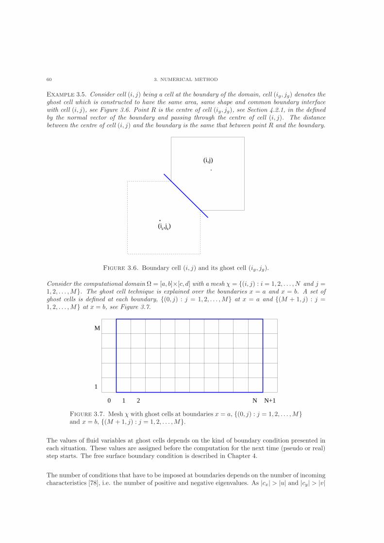
60 3. NUMERICAL METHOD
Example 3.5. Consider cell (i, j) being a cell at the boundary of the domain, cell (ig, jg) denotes theghost cell which is constructed to have the same area, same shape and common boundary interfacewith cell (i, j), see Figure 3.6. Point R is the centre of cell (ig, jg), see Section 4.2.1, in the definedby the normal vector of the boundary and passing through the centre of cell (i, j). The distancebetween the centre of cell (i, j) and the boundary is the same that between point R and the boundary.
(i,j)
(i ,j )gg
Figure 3.6. Boundary cell (i, j) and its ghost cell (ig, jg).
Consider the computational domain Ω = [a, b]×[c, d] with a mesh � = {(i, j) : i = 1, 2, . . . , N and j =1, 2, . . . ,M}. The ghost cell technique is explained over the boundaries x = a and x = b. A set ofghost cells is defined at each boundary, {(0, j) : j = 1, 2, . . . ,M} at x = a and {(M + 1, j) : j =1, 2, . . . ,M} at x = b, see Figure 3.7.
0 2 N+1N1
1
M
Figure 3.7. Mesh � with ghost cells at boundaries x = a, {(0, j) : j = 1, 2, . . . ,M}and x = b, {(M + 1, j) : j = 1, 2, . . . ,M}.
The values of fluid variables at ghost cells depends on the kind of boundary condition presented ineach situation. These values are assigned before the computation for the next time (pseudo or real)step starts. The free surface boundary condition is described in Chapter 4.
The number of conditions that have to be imposed at boundaries depends on the number of incomingcharacteristics [78], i.e. the number of positive and negative eigenvalues. As ∣cx∣ > ∣u∣ and ∣cy∣ > ∣v∣
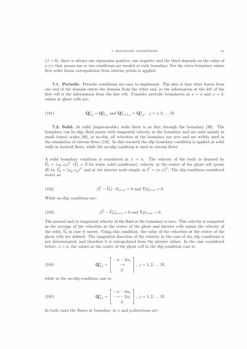
7. BOUNDARY CONDITIONS 61
(� > 0), there is always one eigenvalue positive, one negative and the third depends on the value ofu (v) that means one or two conditions are needed at each boundary. For the extra boundary valuesfirst order linear extrapolation from interior points is applied.
7.1. Periodic. Periodic conditions are easy to implement. The idea is that what leaves fromone end of the domain enters the domain from the other end, so the information at the left of thefirst cell is the information from the last cell. Consider periodic boundaries at x = a and x = b,values at ghost cells are,
Qn0,j = Qn
N,j and QnN+1,j = Qn
1,j , j = 1, 2, . . .M.(181)
7.2. Solid. At solid (impermeable) walls there is no flux through the boundary [39]. Theboundary can be slip, fluid moves with tangential velocity at the boundary and are used mainly insmall (nano) scales [40], or no-slip, all velocities at the boundary are zero and are widely used inthe simulation of viscous flows [116]. In this research the slip boundary condition is applied at solidwalls in inviscid flows, while the no-slip condition is used in viscous flows.
A solid boundary condition is considered at x = a. The velocity of the body is denoted by
Vb = (ub, vb)T (Vb = 0 for static solid conditions), velocity at the centre of the ghost cell (point
R) by Vg = (ug, vg)T and at the interior node simply as V = (u, v)T . The slip condition considered
states as:
(V − Vb) ⋅ n∣x=a = 0 and ∇p∣x=a = 0.(182)
While no-slip conditions are:
(V − Vb)∣x=a = 0 and ∇p∣x=a = 0.(183)
The normal and/or tangential velocity of the fluid at the boundary is zero. This velocity is computedas the average of the velocities at the centre of the ghost and interior cells minus the velocity of
the solid, Vb in case it moves. Using this condition, the value of the velocities at the centre of theghost cells are defined. The tangential direction of the velocity in the case of the slip conditions isnot determinated, and therefore it is extrapolated from the interior values. In the case consideredbefore, x = a, the values at the centre of the ghost cell in the slip condition case is:
Qn0,j =
⎡
⎣
−u− 2ub−vp
⎤
⎦ , j = 1, 2, . . .M,(184)
while in the no-slip condition case is:
Qn0,j =
⎡
⎣
−u− 2ub−v − 2vb
p
⎤
⎦ , j = 1, 2, . . .M.(185)
In both cases the fluxes at boundary in x and y-directions are:
62 3. NUMERICAL METHOD
Fx =
⎡
⎣
�p00
⎤
⎦ and Fy =
⎡
⎣
0�p0
⎤
⎦ .(186)
7.3. Inflow. Fluid enters the domain from the inflow boundary. The velocity of the incoming
fluid Vin = (uin, vin)T will be given to the ghost cell, while the pressure is extrapolated from the
interior points. Consider an inflow condition at boundary x = a,
QnN+1,j =
⎡
⎣
uinvinp1,j
⎤
⎦ , j = 1, 2, . . .M.(187)
So the fluxes at boundaries are:
Fx =
⎡
⎣
u2∗ + �p∗u∗v∗u
⎤
⎦ and Fy =
⎡
⎣
u∗v∗v2∗ + �p∗
v∗
⎤
⎦ ,(188)
where (u∗, v∗, p∗) are the solution of the RP produced by the inflow values and the values at thefirst node.
7.4. Outflow. The condition is set for the fluid to leave the domain freely. The condition atghost cells is obtained by extrapolation from the values at interior points, so the values at the ghostcells depends on the values inside the domain. Consider an outflow condition at boundary x = b,using a simple linear extrapolation (gradients of velocities and pressure to be zero) the conditionsare,
QnN+1,j = Qn
N,j , j = 1, 2, . . .M.(189)
So the fluxes at boundaries are:
Fx =
⎡
⎣
u2N,j + �pN,j
uN,jvN,j
u
⎤
⎦ and Fy =
⎡
⎣
uN,jvN,j
v2N,j + �pN,j
vN,j
⎤
⎦ .(190)
8. Linearization
Now that the flux between cells is known, the aim is to rewrite equation (124) having the unknownsat the LHS and the known values at the RHS. Using the same notation as in equation (124) thisbecomes,
(191)Ω(i,j)
Δ�(I − I0)∂U(i,j) +
Ω(i,j)
ΔtI0∂U(i,j) +
⎛
⎝∑
l∈∂Ω(i,j)
(FS)l −BΩ(i,j)
⎞
⎠
m+1
= −Ω(i,j)
ΔtI0(U
m(i,j) −Un
(i,j)).
8. LINEARIZATION 63
The ideal is the LHS to be a function of {∂Um(k,l) : (k, l) ∈ {(i, j), (i+1, j), (i, j +1), (i− 1, j), (i, j −
1)}}. The flux at pseudo-timem+1 is linearized by writing it as a function of the flux at pseudo-timem using Taylor expansion [71],
Fm+1 = Fm +
(∂F
∂�
)m
Δ� +O[Δ�2],(192)
using the Chain Rule.
(∂F
∂�
)m
=
(∂F
∂U
)m∂U
∂�.(193)
The flux at cell interfaces are the solution of RP depending in the velocities and pressure at bothsides of the interface, so the flux is a function of both states, F = F(UL,UR) and using the ChainRule,
(∂F
∂�
)m
=
(∂F0
∂UL
)m∂UL
∂�+
(∂F0
∂UR
)m∂UR
∂�.(194)
It is possible to approximate ∂UL/∂� and ∂UR/∂� as,
∂UL
∂�=
(UL)m+1 − (UL)m
Δ�≃ ∂UL
Δ�,(195)
∂UR
∂�=
(UR)m+1 − (UR)m
Δ�≃ ∂UR
Δ�,(196)
so equation (194) can be written as,
(∂F
∂�
)m
≃(∂F
∂UL
)m∂UL
Δ�+
(∂F
∂UR
)m∂UR
Δ�.(197)
The partial derivative of the flux is written as a function of the partial derivative of the states ateach side of the interface. Still the Jacobians ∂F/∂UL and ∂F/∂UR are unknowns. The form ofthese Jacobians depends on the RS used, as the expression of the flux change depends on it. Theexpression of the flux using Roe’s RS is given in equation (162), neglecting the terms coming fromthe derivatives of D with respect to UL and UR the Jacobians results,
A+ =∂F0
∂UL≃ 1
2
[A(UL) +D
],(198)
A− =∂F0
∂UR≃ 1
2
[A(UR)−D
].(199)
The expression of the flux using the HLL RS is given in equation (164) and the Jacobians results,
64 3. NUMERICAL METHOD
A+ =∂FHLL
∂UL≃ t2A(U
L) + t3I,(200)
A− =∂FHLL
∂UR≃ t1A(U
R)− t3I.(201)
Then being careful in the expression of A+ and A− used, equation (197) can be written as,
(∂F
∂�
)m
≃ 1
Δ�
[A+∂UL +A−∂UR
],(202)
and applying it to (192),
Fm+1i = Fm
i +A+∂UL +A−∂UR.(203)
The source B from equation (124) can be also linearized as follows,
Bm+1 ≃ Bm +G∂U,(204)
where G = ∂B/∂U. In our case, B = gj, G = diag(0, g, 0)
Then it is possible to write the flux at m+ 1 in function of
(205)
⎛
⎝∑
l∈∂Ω(i,j)
(FS)l −BΩ(i,j)
⎞
⎠
m+1
=
⎛
⎝∑
l∈∂Ω(i,j)
(FS)l −BΩ(i,j)
⎞
⎠
m
+
⎛
⎝∑
l∈∂Ω(i,j)
(∂FS)l
⎞
⎠
m
−G∂U
Using this expression to rewrite equation (191) results,
(206)Ω(i,j)
Δ�(I − I0)∂U(i,j) +
Ω(i,j)
ΔtI0∂U(i,j) +
⎛
⎝∑
l∈∂Ω(i,j)
(∂FS)l
⎞
⎠
m
−G∂U(i,j)
= −Ω(i,j)
ΔtI0(U
m(i,j) −Un
(i,j)) +
⎛
⎝∑
l∈∂Ω(i,j)
(FS)l −BΩ(i,j)
⎞
⎠
m
,
which can be rewritten in compact form as,
Ω
Δ�(I +H) ∂U+
⎛
⎝∑
l∈∂Ω(i,j)
(∂FS)l
⎞
⎠
m
= −R,(207)
9. LINEAR SYSTEM 65
where,
H =
(Δ�
Δt− 1
)
I0 −Δ�I�Gm,(208)
R =Ω
ΔtI0 (U
m −Un) +
⎛
⎝∑
l∈∂Ω(i,j)
(FS)l −BΩ(i,j)
⎞
⎠
m
.(209)
Adding the pseudo-time derivative also to the conservation of momentum, H results
H =Δ�
ΔtI0 −Δ�I�G.(210)
9. Linear System
Equation (206) which is a rewritten version of equation (124) can be extended,
(211)Ω
Δ�(I +H) ∂Uij +
[
A+i+ 1
2 j−A−
i− 12 j
+A+ij+ 1
2
−A−ij− 1
2
]
∂Uij
[
A−i+ 1
2 j∂Ui+1j −A+
i− 12 j∂Ui−1j +A−
ij+ 12
∂Uij+1 −A+ij− 1
2
∂Uij−1
]
= −R,
which is a system with unknown ∂U. Notice the dependency on the RS to write matrices A+ andA−, and obviously the expression of the flux. Once the system (211) is solved and the solution ∂Uis known, the update of the solution in pseudo-time is as simple as,
Um+1 = Um + ∂U.(212)
The system can be written in matrix form with a huge system matrix A, so the solution ∂U beingthe solution of a linear system,
A∂U = R.(213)
Notation 3.6. Define the nonation to be used in the construction of A. When computing cell (i, j):
∙ Ci,j denotes the contribution from ∂Ui,j to the matrix A,
Ci,j =Ω
Δ�(I +H) +
[
A+i+ 1
2 j−A−
i− 12 j
+A+ij+ 1
2
−A−ij− 1
2
]
,(214)
∙ Ri,j denotes the contribution from ∂Ui+1,j to the matrix A,
Ri,j = A−i+ 1
2 j,(215)
∙ Ti,j denotes the contribution from ∂Ui,j+1 to the matrix A,
Ti,j = A−ij+ 1
2
,(216)
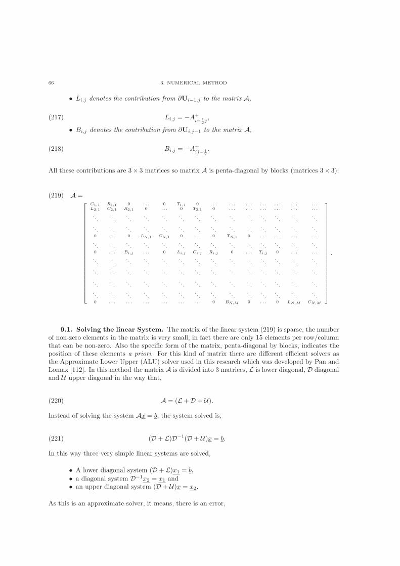
66 3. NUMERICAL METHOD
∙ Li,j denotes the contribution from ∂Ui−1,j to the matrix A,
Li,j = −A+i− 1
2 j,(217)
∙ Bi,j denotes the contribution from ∂Ui,j−1 to the matrix A,
Bi,j = −A+ij− 1
2
.(218)
All these contributions are 3× 3 matrices so matrix A is penta-diagonal by blocks (matrices 3× 3):
(219) A =⎡
⎢⎢⎢⎢⎢⎢⎢⎢⎢⎢⎢⎢⎢⎢⎢⎢⎢⎢⎢⎣
C1,1 R1,1 0 . . . 0 T1,1 0 . . . . . . . . . . . . . . . . . . . . .L2,1 C2,1 R2,1 0 . . . 0 T2,1 0 . . . . . . . . . . . . . . . . . .
. . .. . .
. . .. . .
. . .. . .
. . .. . .
. . .. . .
. . .. . .
. . .. . .
. . .. . .
. . .. . .
. . .. . .
. . .. . .
. . .. . .
. . .. . .
. . .. . .
0 . . . 0 LN,1 CN,1 0 . . . 0 TN,1 0 . . . . . . . . . . . .
. . .. . .
. . .. . .
. . .. . .
. . .. . .
. . .. . .
. . .. . .
. . .. . .
0 . . . Bi,j . . . 0 Li,j Ci,j Ri,j 0 . . . Ti,j 0 . . . . . .
. . .. . .
. . .. . .
. . .. . .
. . .. . .
. . .. . .
. . .. . .
. . .. . .
. . .. . .
. . .. . .
. . .. . .
. . .. . .
. . .. . .
. . .. . .
. . .. . .
. . .. . .
. . .. . .
. . .. . .
. . .. . .
. . .. . .
. . .. . .
. . .. . .
. . .. . .
. . .. . .
. . .. . .
. . .. . .
. . .. . .
. . .. . .
. . .. . .
0 . . . . . . . . . . . . . . . . . . 0 BN,M 0 . . . 0 LN,M CN,M
⎤
⎥⎥⎥⎥⎥⎥⎥⎥⎥⎥⎥⎥⎥⎥⎥⎥⎥⎥⎥⎦
.
9.1. Solving the linear System. The matrix of the linear system (219) is sparse, the numberof non-zero elements in the matrix is very small, in fact there are only 15 elements per row/columnthat can be non-zero. Also the specific form of the matrix, penta-diagonal by blocks, indicates theposition of these elements a priori. For this kind of matrix there are different efficient solvers asthe Approximate Lower Upper (ALU) solver used in this research which was developed by Pan andLomax [112]. In this method the matrix A is divided into 3 matrices, ℒ is lower diagonal, D diagonaland U upper diagonal in the way that,
A = (ℒ+D + U).(220)
Instead of solving the system Ax = b, the system solved is,
(D + ℒ)D−1(D + U)x = b.(221)
In this way three very simple linear systems are solved,
∙ A lower diagonal system (D + ℒ)x1 = b,
∙ a diagonal system D−1x2 = x1 and∙ an upper diagonal system (D + U)x = x2.
As this is an approximate solver, it means, there is an error,
10. SOLUTION SCHEME 67
(222) (D + ℒ)D−1(D + U) = (D + ℒ)(I +D−1U) =D + ℒ+ U + ℒD−1U = A+ ℒD−1U ,
so instead of solving Ax = b, the linear system solved is (A+ℒD−1U)x = b, and the error produced(very small in iterative processes) by this method is:
∣∣(ℒD−1U)x∣∣2.(223)
The structure of matrix A is changed when periodic boundary conditions are used. In this casethe matrix becomes hepta-diagonal because the contribution at left of the first node is given by thelast node. To solve this kind of systems, an external library (HSL MA48) provided by the HarwellSubroutine Library [9] is used.
10. Solution Scheme
The solution procedure used in this dissertation uses the following scheme (similar to [70]):
(1) Define tmax and �max as limit (upper bounds) of real time and pseudo-time iterations andthe tolerance tol,
(2) input the values of the variables at the initial condition (n = 0),(3) initialize the value of the variables at initial pseudo-time (m = 0), i.e., Un,0 = Un,(4) compute Un,m+1 according to (207), and update m to m + 1 until for an index M
∣∣Un,M −Un,M−1∣∣2 < tol or m = �max (then M is defined as �max),(5) update the real time solution Un+1 to the value Un,M (Um+1 → Un+1,m+ 1 → ∞) and
advance the time step from n to n+ 1,(6) repeat from 3 to 5 until n = tmax.

CHAPTER 4
Free Surface
1. Introduction
The free surface is a boundary that moves according to the flow conditions. The position of the freesurface is known at the initial time and its evolution has to be found using flow properties. The freesurface defines an upper boundary for the computational domain for the flow. In Chapter 2 it hasbeen shown how to adjust the grid to the computational domain while in Chapter 3 a descriptionof the method to solve for the incompressible NSE has been presented. The methods applied in theliterature to describe the movement of the free surface and the boundary conditions applied thereare described in this chapter.
To solve a PDE one has to know the domain where the PDE will be solved. In the case of a freesurface this is not a simple fact, since the free surface will move with time and consequently thedomain changes with time. Let’s define the free surface as,
{(x, y, z : t) such that z = �(x, y; t)} ,(224)
then it is possible to write the domain as,
D(x, y, z; t) = [x0, xend]× [y0, yend]× [0, �(x, y; t)]× [t0, tend](225)
An idea for the solution procedure using the CCCM and ACM follows the scheme:
(1) Build the mesh fitting the domain.(2) Compute the pressure and the velocity until convergence in pseudo-time is reached.(3) Move the free surface, according to the velocity vectors (at the new real time) at the free
surface.(4) Repeat from 1 to 3 until the steady state or the end of the computation is reached.
There are in the literature different methods to locate the free surface (step 3) and therefore toidentify the new domain. These methods can be divided into the following categories [39, 125]:
∙ Interface Tracking Methods. These methods focus their attention directly in the evolutionin time of the position of the free surface. The position of the fluid which producesthe movement of the free surface is not considered. This methods require moving gridsadjusting to the free surface. Some of those methods are the Height Function or theArbitrary Lagrangian-Eulerian (ALE) Method. “The leading question of Interface Trackingmethods is: where is the surface?” [125].
∙ Interface Capturing Methods, also known as Volume Capturing Methods. These other setof methods compute indirectly the position of the free surface. In a first stage the newposition of the fluid is computed, not paying any attention to the free surface, and in a
69
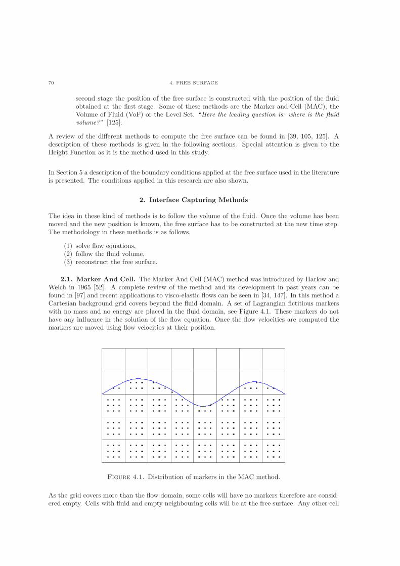
70 4. FREE SURFACE
second stage the position of the free surface is constructed with the position of the fluidobtained at the first stage. Some of these methods are the Marker-and-Cell (MAC), theVolume of Fluid (VoF) or the Level Set. “Here the leading question is: where is the fluidvolume?” [125].
A review of the different methods to compute the free surface can be found in [39, 105, 125]. Adescription of these methods is given in the following sections. Special attention is given to theHeight Function as it is the method used in this study.
In Section 5 a description of the boundary conditions applied at the free surface used in the literatureis presented. The conditions applied in this research are also shown.
2. Interface Capturing Methods
The idea in these kind of methods is to follow the volume of the fluid. Once the volume has beenmoved and the new position is known, the free surface has to be constructed at the new time step.The methodology in these methods is as follows,
(1) solve flow equations,(2) follow the fluid volume,(3) reconstruct the free surface.
2.1. Marker And Cell. The Marker And Cell (MAC) method was introduced by Harlow andWelch in 1965 [52]. A complete review of the method and its development in past years can befound in [97] and recent applications to visco-elastic flows can be seen in [34, 147]. In this method aCartesian background grid covers beyond the fluid domain. A set of Lagrangian fictitious markerswith no mass and no energy are placed in the fluid domain, see Figure 4.1. These markers do nothave any influence in the solution of the flow equation. Once the flow velocities are computed themarkers are moved using flow velocities at their position.
Figure 4.1. Distribution of markers in the MAC method.
As the grid covers more than the flow domain, some cells will have no markers therefore are consid-ered empty. Cells with fluid and empty neighbouring cells will be at the free surface. Any other cell
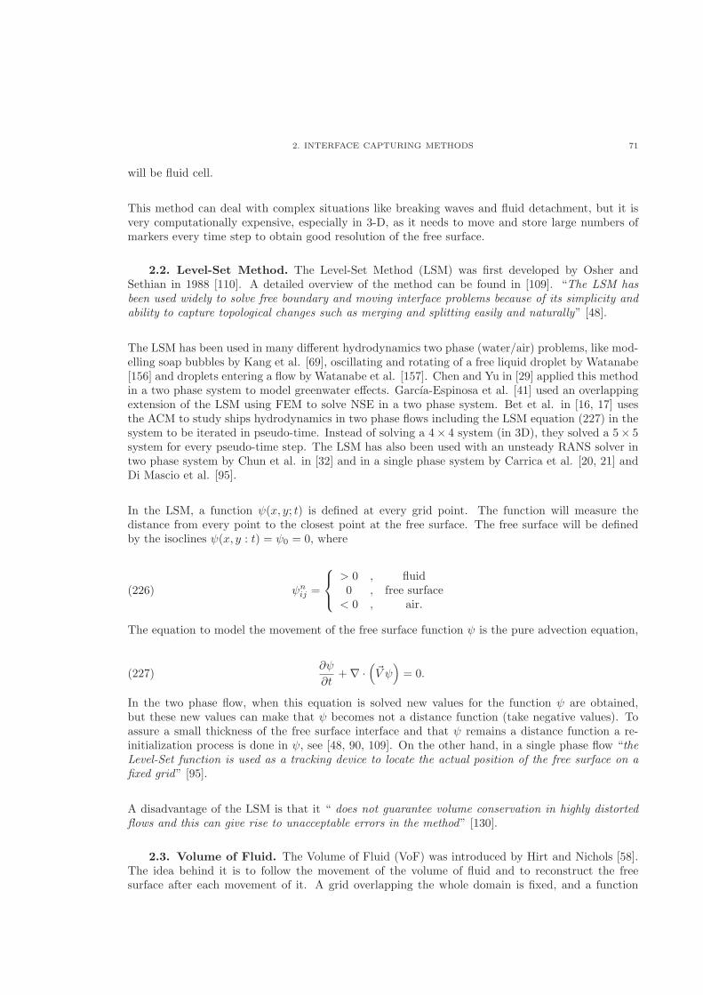
2. INTERFACE CAPTURING METHODS 71
will be fluid cell.
This method can deal with complex situations like breaking waves and fluid detachment, but it isvery computationally expensive, especially in 3-D, as it needs to move and store large numbers ofmarkers every time step to obtain good resolution of the free surface.
2.2. Level-Set Method. The Level-Set Method (LSM) was first developed by Osher andSethian in 1988 [110]. A detailed overview of the method can be found in [109]. “The LSM hasbeen used widely to solve free boundary and moving interface problems because of its simplicity andability to capture topological changes such as merging and splitting easily and naturally” [48].
The LSM has been used in many different hydrodynamics two phase (water/air) problems, like mod-elling soap bubbles by Kang et al. [69], oscillating and rotating of a free liquid droplet by Watanabe[156] and droplets entering a flow by Watanabe et al. [157]. Chen and Yu in [29] applied this methodin a two phase system to model greenwater effects. Garcıa-Espinosa et al. [41] used an overlappingextension of the LSM using FEM to solve NSE in a two phase system. Bet et al. in [16, 17] usesthe ACM to study ships hydrodynamics in two phase flows including the LSM equation (227) in thesystem to be iterated in pseudo-time. Instead of solving a 4× 4 system (in 3D), they solved a 5× 5system for every pseudo-time step. The LSM has also been used with an unsteady RANS solver intwo phase system by Chun et al. in [32] and in a single phase system by Carrica et al. [20, 21] andDi Mascio et al. [95].
In the LSM, a function (x, y; t) is defined at every grid point. The function will measure thedistance from every point to the closest point at the free surface. The free surface will be definedby the isoclines (x, y : t) = 0 = 0, where
nij =
⎧
⎨
⎩
> 0 , fluid0 , free surface< 0 , air.
(226)
The equation to model the movement of the free surface function is the pure advection equation,
∂
∂t+∇ ⋅
(
V )
= 0.(227)
In the two phase flow, when this equation is solved new values for the function are obtained,but these new values can make that becomes not a distance function (take negative values). Toassure a small thickness of the free surface interface and that remains a distance function a re-initialization process is done in , see [48, 90, 109]. On the other hand, in a single phase flow “theLevel-Set function is used as a tracking device to locate the actual position of the free surface on afixed grid” [95].
A disadvantage of the LSM is that it “ does not guarantee volume conservation in highly distortedflows and this can give rise to unacceptable errors in the method” [130].
2.3. Volume of Fluid. The Volume of Fluid (VoF) was introduced by Hirt and Nichols [58].The idea behind it is to follow the movement of the volume of fluid and to reconstruct the freesurface after each movement of it. A grid overlapping the whole domain is fixed, and a function
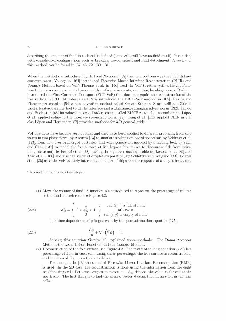
72 4. FREE SURFACE
describing the amount of fluid in each cell is defined (some cells will have no fluid at all). It can dealwith complicated configurations such as breaking waves, splash and fluid detachment. A review ofthis method can be found in [37, 43, 72, 130, 131].
When the method was introduced by Hirt and Nichols in [58] the main problem was that VoF did notconserve mass. Youngs in [164] introduced Piecewise-Linear Interface Reconstruction (PLIR) andYoung’s Method based on VoF. Thomas et al. in [146] used the VoF together with a Height Func-tion that conserves mass and allows smooth surface movements, excluding breaking waves. Rudmanintroduced the Flux-Corrected Transport (FCT-VoF) that does not require the reconstruction of thefree surface in [130]. Muzaferija and Peric introduced the HRIC-VoF method in [105]. Harvie andFletcher presented in [54] a new advection method called Stream Scheme. Scardovelli and Zaleskiused a least-square method to fit the interface and a Eulerian-Lagrangian advection in [132]. Pilliodand Puckett in [68] introduced a second order scheme called ELVIRA, which is second order. Lopezet al. applied spline to the interface reconstruction in [88]. Tang et al. [145] applied PLIR in 3-Dalso Lopez and Hernandez [87] provided methods for 3-D general grids.
VoF methods have become very popular and they have been applied to different problems, from shipwaves in two phase flows, by Azcueta [13] to simulate sloshing on board spacecraft by Veldman et al.[153], from flow over submerged obstacles, and wave generation induced by a moving bed, by Shenand Chan [137] to model the free surface at fish bypass (structures to discourage fish from swim-ming upstream), by Ferrari et al. [38] passing through overtopping problems, Losada et al. [89] andXiao et al. [160] and also the study of droplet evaporation, by Schlottke and Weigand[133]. Lohneret al. [85] used the VoF to study interaction of a fleet of ships and the response of a ship in heavy sea.
This method comprises two steps:
(1) Move the volume of fluid. A function � is introduced to represent the percentage of volumeof the fluid in each cell, see Figure 4.2,
�nij =
⎧
⎨
⎩
1 , cell (i, j) is full of fluid0 < �nij < 1 , otherwise
0 , cell (i, j) is empty of fluid.(228)
The time dependence of � is governed by the pure advenction equation [125],
∂�
∂t+∇ ⋅
(
V �)
= 0.(229)
Solving this equation Gerrits [43] explained three methods. The Donor-AcceptorMethod, the Local Height Function and the Youngs’ Method.
(2) Reconstruction of the free surface, see Figure 4.3. The result of solving equation (229) is apercentage of fluid in each cell. Using these percentages the free surface is reconstructed,and there are different methods to do so.
For example, in [43] the so-called Piecewise-Linear Interface Reconstruction (PLIR)is used. In the 2D case, the reconstruction is done using the information from the eightneighbouring cells. Let’s use compass notation, i.e. �ne denotes the value at the cell at thenorth east. The first thing is to find the normal vector n using the information in the ninecells.
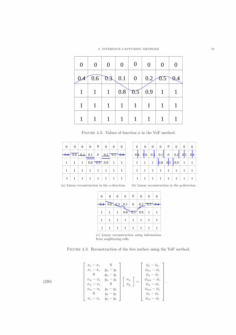
2. INTERFACE CAPTURING METHODS 73
0.30.4 0.6 0.1
0.5 0.9
0.2 0.5 0.4
0 0 0 00000
0
11
1
1 1 1 1 1
1
11
11
11
11
11
11
0.8
Figure 4.2. Values of function � in the VoF method.
0.30.4 0.6 0.1
0.5 0.9
0.2 0.5 0.4
0 0 0 00000
0
1
1 1 1 1 1
1
11
11
11
1111
0.8
1111
(a) Linear reconstruction in the x-direction.
0.30.4 0.6 0.1
0.5 0.9
0.2 0.5 0.4
0 0 0 00000
0
1
1 1 1 1 1
1
11
11
11
1111
0.8
1111
(b) Linear reconstruction in the y-direction.
0.30.4 0.6 0.1
0.5 0.9
0.2 0.5 0.4
0 0 0 00000
0
1
1 1 1 1 1
1
11
11
11
1111
0.8
1111
(c) Linear reconstruction using informationfrom neighboring cells.
Figure 4.3. Reconstruction of the free surface using the VoF method.
⎡
⎢⎢⎢⎢⎢⎢⎢⎢⎢⎢⎣
xe − xc 0xe − xc yn − yc
0 yn − ycxw − xc yn − ycxw − xc 0xw − xc ys − yc
0 ys − ycxe − xc ys − yc
⎤
⎥⎥⎥⎥⎥⎥⎥⎥⎥⎥⎦
[nxny
]
=
⎡
⎢⎢⎢⎢⎢⎢⎢⎢⎢⎢⎣
�e − �c�ne − �c�n − �c�nw − �c�w − �c�sw − �c�s − �c�se − �c
⎤
⎥⎥⎥⎥⎥⎥⎥⎥⎥⎥⎦
.(230)
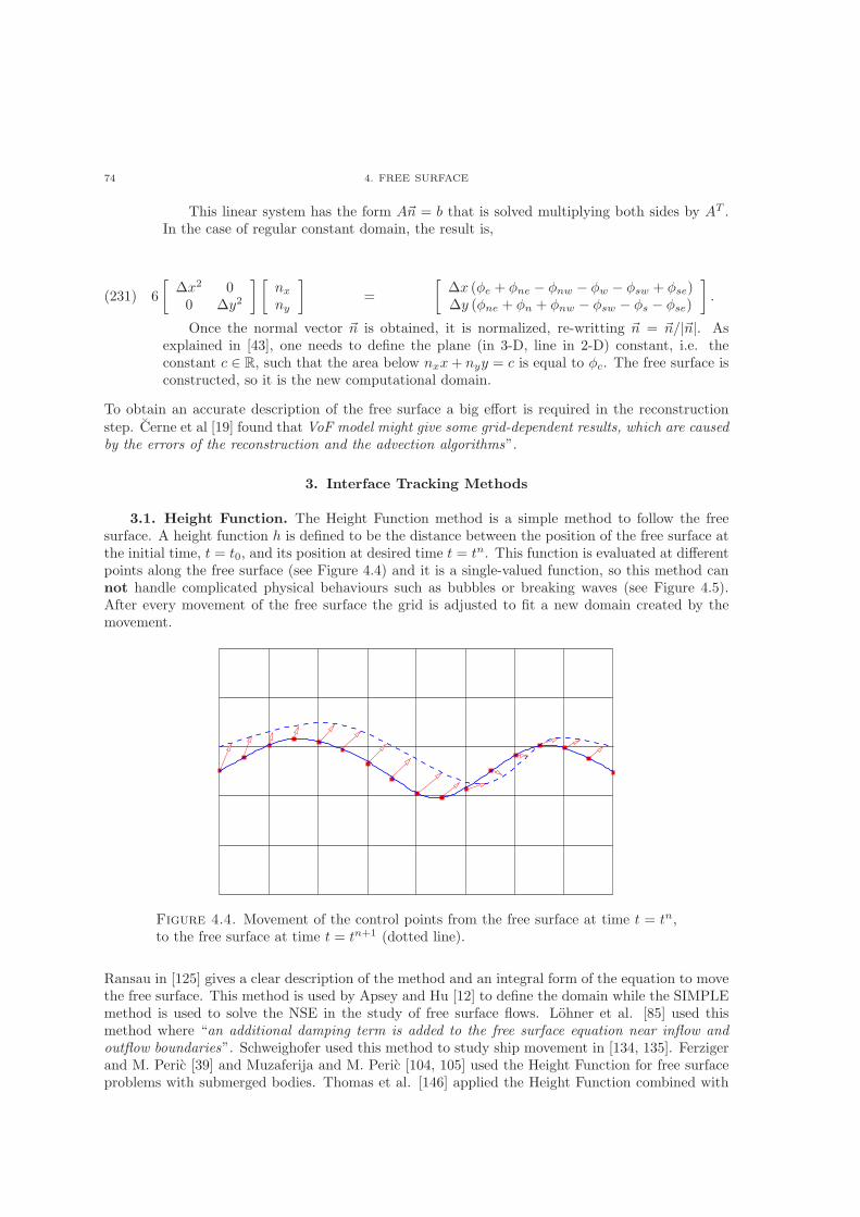
74 4. FREE SURFACE
This linear system has the form An = b that is solved multiplying both sides by AT .In the case of regular constant domain, the result is,
(231) 6
[Δx2 00 Δy2
] [nxny
]
=
[Δx (�e + �ne − �nw − �w − �sw + �se)Δy (�ne + �n + �nw − �sw − �s − �se)
]
.
Once the normal vector n is obtained, it is normalized, re-writting n = n/∣n∣. Asexplained in [43], one needs to define the plane (in 3-D, line in 2-D) constant, i.e. theconstant c ∈ ℝ, such that the area below nxx+ nyy = c is equal to �c. The free surface isconstructed, so it is the new computational domain.
To obtain an accurate description of the free surface a big effort is required in the reconstructionstep. Cerne et al [19] found that VoF model might give some grid-dependent results, which are causedby the errors of the reconstruction and the advection algorithms”.
3. Interface Tracking Methods
3.1. Height Function. The Height Function method is a simple method to follow the freesurface. A height function ℎ is defined to be the distance between the position of the free surface atthe initial time, t = t0, and its position at desired time t = tn. This function is evaluated at differentpoints along the free surface (see Figure 4.4) and it is a single-valued function, so this method cannot handle complicated physical behaviours such as bubbles or breaking waves (see Figure 4.5).After every movement of the free surface the grid is adjusted to fit a new domain created by themovement.
Figure 4.4. Movement of the control points from the free surface at time t = tn,to the free surface at time t = tn+1 (dotted line).
Ransau in [125] gives a clear description of the method and an integral form of the equation to movethe free surface. This method is used by Apsey and Hu [12] to define the domain while the SIMPLEmethod is used to solve the NSE in the study of free surface flows. Lohner et al. [85] used thismethod where “an additional damping term is added to the free surface equation near inflow andoutflow boundaries”. Schweighofer used this method to study ship movement in [134, 135]. Ferzigerand M. Peric [39] and Muzaferija and M. Peric [104, 105] used the Height Function for free surfaceproblems with submerged bodies. Thomas et al. [146] applied the Height Function combined with
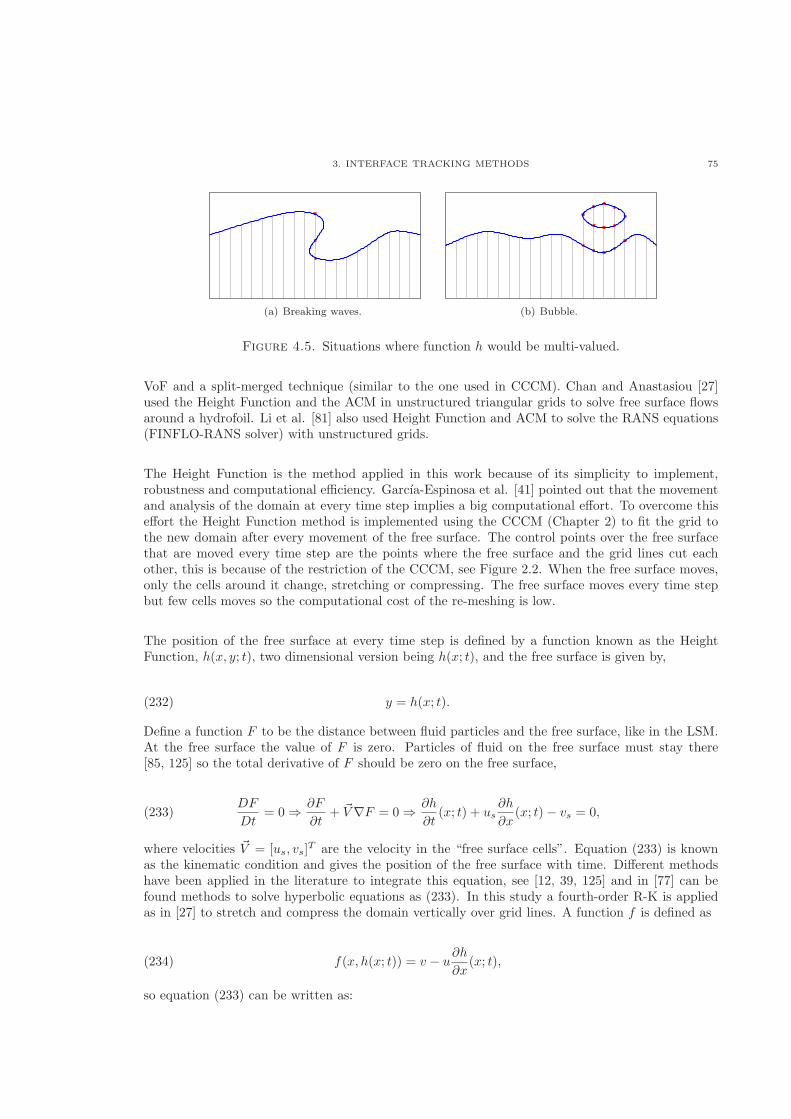
3. INTERFACE TRACKING METHODS 75
(a) Breaking waves. (b) Bubble.
Figure 4.5. Situations where function ℎ would be multi-valued.
VoF and a split-merged technique (similar to the one used in CCCM). Chan and Anastasiou [27]used the Height Function and the ACM in unstructured triangular grids to solve free surface flowsaround a hydrofoil. Li et al. [81] also used Height Function and ACM to solve the RANS equations(FINFLO-RANS solver) with unstructured grids.
The Height Function is the method applied in this work because of its simplicity to implement,robustness and computational efficiency. Garcıa-Espinosa et al. [41] pointed out that the movementand analysis of the domain at every time step implies a big computational effort. To overcome thiseffort the Height Function method is implemented using the CCCM (Chapter 2) to fit the grid tothe new domain after every movement of the free surface. The control points over the free surfacethat are moved every time step are the points where the free surface and the grid lines cut eachother, this is because of the restriction of the CCCM, see Figure 2.2. When the free surface moves,only the cells around it change, stretching or compressing. The free surface moves every time stepbut few cells moves so the computational cost of the re-meshing is low.
The position of the free surface at every time step is defined by a function known as the HeightFunction, ℎ(x, y; t), two dimensional version being ℎ(x; t), and the free surface is given by,
y = ℎ(x; t).(232)
Define a function F to be the distance between fluid particles and the free surface, like in the LSM.At the free surface the value of F is zero. Particles of fluid on the free surface must stay there[85, 125] so the total derivative of F should be zero on the free surface,
DF
Dt= 0 ⇒ ∂F
∂t+ V∇F = 0 ⇒ ∂ℎ
∂t(x; t) + us
∂ℎ
∂x(x; t)− vs = 0,(233)
where velocities V = [us, vs]T are the velocity in the “free surface cells”. Equation (233) is known
as the kinematic condition and gives the position of the free surface with time. Different methodshave been applied in the literature to integrate this equation, see [12, 39, 125] and in [77] can befound methods to solve hyperbolic equations as (233). In this study a fourth-order R-K is appliedas in [27] to stretch and compress the domain vertically over grid lines. A function f is defined as
f(x, ℎ(x; t)) = v − u∂ℎ
∂x(x; t),(234)
so equation (233) can be written as:
76 4. FREE SURFACE
∂ℎ
∂t= f(x, ℎ(x; t)).(235)
The R-K used is a four stage method (K ′s), which is explicit, fourth-order and very popular becauseof the simplicity of the coefficients to compute its stages [96].
⎧
⎨
⎩
K1 = f(xi;ℎni )
K2 = f(xi + (Δt/2);ℎni + (Δt/2)K1)K3 = f(xi + (Δt/2);ℎni + (Δt/2)K2)K4 = f(xi +Δt;ℎni +ΔtK3)ℎn+1i = ℎni + (Δt/6)(K1 + 2K2 + 2K3 +K4).
(236)
This method has four stages, so instead of computing time t = tn+1 directly from time t = tn, threeintermediate positions of the free surface are required before the definitive position at the new timestep is computed. A scheme of the time integration of the free surface used in this dissertation is:
(1) First R-K step(a) Call the CCCR to define the mesh using the free surface position ℎn.(b) Call the pseudo time iteration.(c) Compute K1,
K1 = f(tn, ℎn).(237)
(d) Move the free surface
ℎn,★ = ℎn +Δt
2K1.(238)
(2) Second R-K step(a) Call the CCCR to define the mesh using the free surface position ℎn,★.(b) Call the pseudo time iteration.(c) Compute K2,
K2 = f
(
tn +Δt
2, ℎn,★
)
.(239)
(d) Move the free surface
ℎn,★★ = ℎn +Δt
2K2.(240)
(3) Third R-K step(a) Call the CCCR to define the mesh using the free surface position ℎn,★★.(b) Call the pseudo time iteration.(c) Compute K3,
K3 = f
(
tn +Δt
2, ℎn,★★
)
.(241)
(d) Move the free surface
ℎn,★★★ = ℎn +ΔtK3.(242)
3. INTERFACE TRACKING METHODS 77
(4) Fourth R-K step(a) Call the CCCR to define the mesh using the free surface position ℎn,★★★.(b) Call the pseudo time iteration.(c) Compute K4,
K4 = f (tn +Δt, ℎn,★★★) .(243)
(d) Update the free surface on time t = tn+1
ℎn+1 = ℎn +Δt
6(K1 + 2K2 + 2K3 +K4).(244)
3.2. Arbitrary Lagrangian-Eulerian Methods. There are two different approaches in thestudy of fluids. Eulerian (MAC, LSM and VoF) methods where attention is paid to volume spacesand the fluid at these volumes is studied on time and the Lagrangian (Height Function) methodswhere a fluid fraction/particle is followed on time. Each set of methods has their own problems. La-grangian methods can not deal with complicated shapes for the free surface while Eulerian methodscan deal with complicated shapes but are less accurate on the definition of the free surface. TheArbitrary Lagrangian-Eulerian (ALE) Methods try to combine both techniques obtaining a methodthat overcomes the weakness of each method. The mesh is moving, adjusting itself to the free sur-face, but the velocity of the free surface is unknown a priori, and also the velocity of the mesh. Adescription of this method given by Souli and Zolesio can be found in [142].
Lipari and Napoli [83] and Lo and Young [84] applied ALE method to free surface problems. Onateet al. [111] applied the three methodologies, Eulerian, Lagrangian and ALE, to free surface flowsand fluid-structure interaction. Del Pin et al. [115] applied an extension of the ALE method alsoto free surface flows and fluid-structure interaction. Li et al. [80] studied free surface problems andbubble dynamics using this method. ALE methods have been used also in bio-medical problems, forexample, Quarteroni in [121] applied the method to the flow in the heart, arteries and veins studyingcardiovascular diseases.
It can be said that the ALE method being a combination of both methods follows what happens ina volume space and in a fluid fraction/particle. Two different sets of equations are required, one forthe movement of the fluid and one for the movement of the grid. A convective velocity c is defined as
the difference between the fluid velocity V and the mesh velocity V mesℎ. Eulerian methods consider
mesh velocity V mesℎ = 0, in Lagrangian methods the mesh moves with the fluid at same velocity,so c = 0, while in ALE methods the velocity of the mesh is arbitrary but different than zero and the
velocity of the fluid, V mesℎ ∕= 0 and V mesℎ ∕= V [125, 142].
The incompressible NSE (106,107) in Eulerian form looks like,
{
∇ ⋅ V = 0∂V∂t +∇ ⋅
(
V × V − T)
= B.(245)
While in the ALE formulation the mesh velocity V mesℎ is added to the transport term in themomentum equation [111] obtaining,
78 4. FREE SURFACE
{
∇ ⋅ V = 0∂V∂t +∇ ⋅
((
V − V mesℎ)
× V − T)
= B.(246)
Dependence between the coordinates and the moving grid have to been considered before solvingthese equations, see details in [115].
4. Pressure on Free Surface Flows
In flows not involving a free surface the gravity force effects have been neglected, so the source termin the conservation of momentum equation is B = 0. But for free surface flows the gravity plays animportant role and the conservation of momentum equation is,
(247)∂V
∂t+
∂
∂x
[u2 + puv
]
+∂
∂y
[uv
v2 + p
]
− 1
Re
(∂
∂x
[uxvx
]
+∂
∂y
[uyvy
])
= B =
[0�g
]
.
The pressure (dynamic pressure) can be divided into static (or kinematic) pressure ps and thehydrostatic pressure pℎ [27],
p = ps + pℎ = ps + �gℎ,(248)
where ℎ is the free surface position, g the gravity force and � the density. In the above formulationthe pressure is derived by x and y,
∂p
∂x=∂ps∂x
+�gℎ
∂x=∂ps∂x
+ g�ℎ
∂x=∂ps∂x
+ �gSx =∂ps∂x
+ Sx/Fr2.(249)
∂p
∂y=∂ps∂y
+�gℎ
∂y=∂ps∂y
+ gℎℎ
∂y=∂ps∂x
+ �g.(250)
Sx being the gradient of the free surface, Fr the Froude number and ℎ the position in the y-direction,which derived in the y-direction is the unit. Combining equations (247,249,250) the result is,
(251)∂V
∂t+
∂
∂x
[u2 + psuv
]
+∂
∂y
[uv
v2 + ps
]
− 1
Re
(∂
∂x
[uxvx
]
+∂
∂y
[uyvy
])
= B =
[−Sx/Fr
2
�g − �g
]
=
[−Sx/Fr
2
0
]
.
5. Boundary Conditions at the Free Surface
In the literature some work for the free surface has been done using two phase fluids [13, 71, 117, 119]where the free surface is just an interface between two different fluids. While in one phase fluid[12, 37, 39, 72, 73, 85, 134, 135, 136] the free surface is a moving boundary and therefore boundary
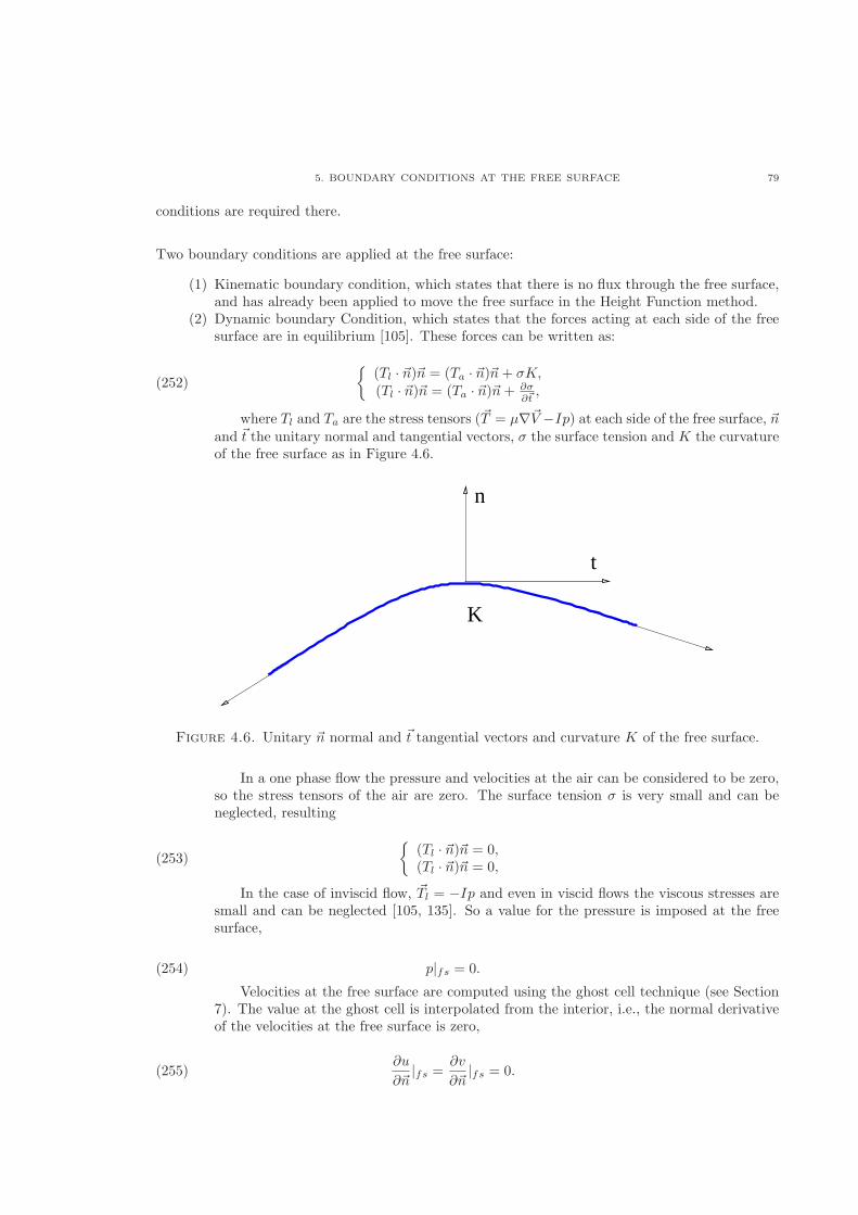
5. BOUNDARY CONDITIONS AT THE FREE SURFACE 79
conditions are required there.
Two boundary conditions are applied at the free surface:
(1) Kinematic boundary condition, which states that there is no flux through the free surface,and has already been applied to move the free surface in the Height Function method.
(2) Dynamic boundary Condition, which states that the forces acting at each side of the freesurface are in equilibrium [105]. These forces can be written as:
{(Tl ⋅ n)n = (Ta ⋅ n)n+ �K,(Tl ⋅ n)n = (Ta ⋅ n)n+ ∂�
∂t,
(252)
where Tl and Ta are the stress tensors (T = �∇V −Ip) at each side of the free surface, nand t the unitary normal and tangential vectors, � the surface tension and K the curvatureof the free surface as in Figure 4.6.
t
n
K
Figure 4.6. Unitary n normal and t tangential vectors and curvature K of the free surface.
In a one phase flow the pressure and velocities at the air can be considered to be zero,so the stress tensors of the air are zero. The surface tension � is very small and can beneglected, resulting
{(Tl ⋅ n)n = 0,(Tl ⋅ n)n = 0,
(253)
In the case of inviscid flow, Tl = −Ip and even in viscid flows the viscous stresses aresmall and can be neglected [105, 135]. So a value for the pressure is imposed at the freesurface,
p∣fs = 0.(254)
Velocities at the free surface are computed using the ghost cell technique (see Section7). The value at the ghost cell is interpolated from the interior, i.e., the normal derivativeof the velocities at the free surface is zero,
∂u
∂n∣fs =
∂v
∂n∣fs = 0.(255)
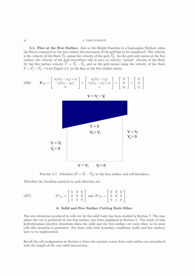
80 4. FREE SURFACE
5.1. Flux at the Free Surface. Just as the Height Function is a Lagrangian Method, whenthe flux is computed at the free surface the movement of the grid has to be considered. The velocity
is the velocity of the fluid, Vf , minus the velocity of the grid, Vg. As the grid only moves at the freesurface, the velocity of the grid everywhere else is zero, so velocity “means” velocity of the fluid.
At the free surface velocity V = Vf − Vg, and as the grid moves using the velocity of the fluid,
V = Vf − Vg = 0 see Figure 4.7, so the flux at the free surface states,
F∣fs =
⎡
⎣
uf (uf − ug) + pvf (uf − ug)
u
⎤
⎦+
⎡
⎣
uf (vf − vg)vf (vf − vg) + p
v
⎤
⎦ =
⎡
⎣
00uf
⎤
⎦+
⎡
⎣
00vf
⎤
⎦ .(256)
V = 0V = Vf
g
V = V
V = 0
V = 0V = V
V = V V = 0
fg
g
g
f
f
V = V − Vf g
Figure 4.7. Velocities (V = Vf − Vg) at the free surface and cell interfaces.
Therefore the Jacobian matrices in each direction are:
Ax∣fs =
⎡
⎣
0 0 00 0 01 0 0
⎤
⎦ and Ay∣fs =
⎡
⎣
0 0 00 0 00 1 0
⎤
⎦ .(257)
6. Solid and Free Surface Cutting Each Other
The new situations produced in cells cut by the solid body has been studied in Section 7. The casewhere the cut is produced by the free surface, has been explained in Section 5. The study of shiphydrodynamics involves situations when the solid and the free surface cut each other, so in somecells this situation is presented. For these cells both boundary conditions (solid and free surface)have to be implemented.
Recall the cell configuration in Section 4 where the normal vectors from each surface are normalizedwith the length of the cuts until intersection.
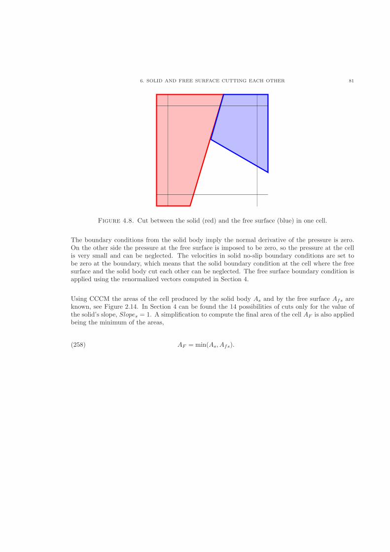
6. SOLID AND FREE SURFACE CUTTING EACH OTHER 81
Figure 4.8. Cut between the solid (red) and the free surface (blue) in one cell.
The boundary conditions from the solid body imply the normal derivative of the pressure is zero.On the other side the pressure at the free surface is imposed to be zero, so the pressure at the cellis very small and can be neglected. The velocities in solid no-slip boundary conditions are set tobe zero at the boundary, which means that the solid boundary condition at the cell where the freesurface and the solid body cut each other can be neglected. The free surface boundary condition isapplied using the renormalized vectors computed in Section 4.
Using CCCM the areas of the cell produced by the solid body As and by the free surface Afs areknown, see Figure 2.14. In Section 4 can be found the 14 possibilities of cuts only for the value ofthe solid’s slope, Slopes = 1. A simplification to compute the final area of the cell AF is also appliedbeing the minimum of the areas,
AF = min(As, Afs).(258)

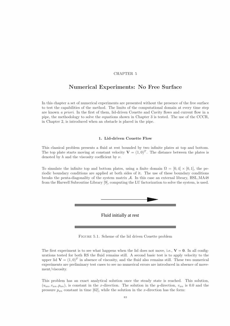
CHAPTER 5
Numerical Experiments: No Free Surface
In this chapter a set of numerical experiments are presented without the presence of the free surfaceto test the capabilities of the method. The limits of the computational domain at every time stepare known a priori. In the first of them, lid-driven Couette and Cavity flows and current flow in apipe, the methodology to solve the equations shown in Chapter 3 is tested. The use of the CCCR,in Chapter 2, is introduced when an obstacle is placed in the pipe.
1. Lid-driven Couette Flow
This classical problem presents a fluid at rest bounded by two infinite plates at top and bottom.The top plate starts moving at constant velocity V = (1, 0)T . The distance between the plates isdenoted by ℎ and the viscosity coefficient by �.
To simulate the infinite top and bottom plates, using a finite domain Ω = [0, 4] × [0, 1], the pe-riodic boundary conditions are applied at both sides of it. The use of these boundary conditionsbreaks the penta-diagonality of the system matrix A. In this case an external library, HSL MA48from the Harwell Subroutine Library [9], computing the LU factorization to solve the system, is used.
��������������������
��������������������
Fluid initially at rest
Figure 5.1. Scheme of the lid driven Couette problem
The first experiment is to see what happens when the lid does not move, i.e., V = 0. In all config-urations tested for both RS the fluid remains still. A second basic test is to apply velocity to theupper lid V = (1, 0)T in absence of viscosity, and the fluid also remains still. These two numericalexperiments are preliminary test cases to see no numerical errors are introduced in absence of move-ment/viscosity.
This problem has an exact analytical solution once the steady state is reached. This solution,(uan, van, pan), is constant in the x-direction. The solution in the y-direction, van is 0.0 and thepressure pan constant in time [62], while the solution in the x-direction has the form:
83
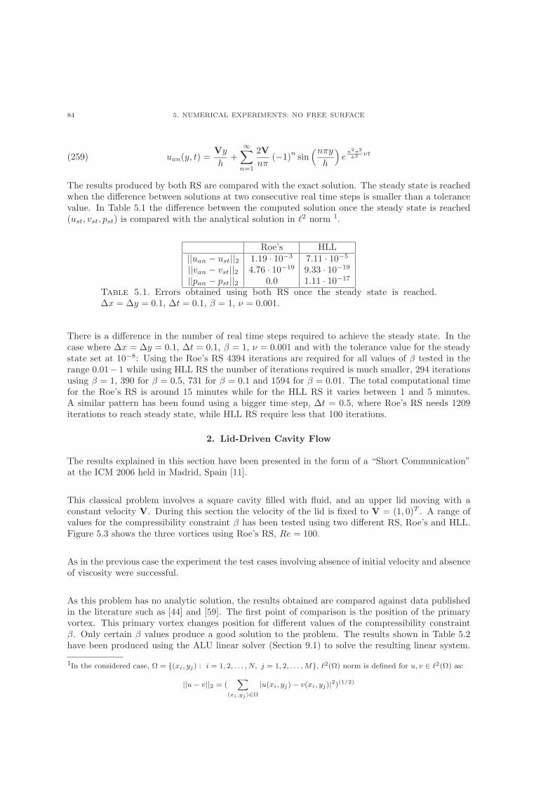
84 5. NUMERICAL EXPERIMENTS: NO FREE SURFACE
(259) uan(y, t) =Vy
ℎ+
∞∑
n=1
2V
n�(−1)
nsin(n�y
ℎ
)
en2�2
ℎ2 �t
The results produced by both RS are compared with the exact solution. The steady state is reachedwhen the difference between solutions at two consecutive real time steps is smaller than a tolerancevalue. In Table 5.1 the difference between the computed solution once the steady state is reached(ust, vst, pst) is compared with the analytical solution in ℓ2 norm 1.
Roe’s HLL∣∣uan − ust∣∣2 1.19 ⋅ 10−3 7.11 ⋅ 10−5
∣∣van − vst∣∣2 4.76 ⋅ 10−19 9.33 ⋅ 10−19
∣∣pan − pst∣∣2 0.0 1.11 ⋅ 10−17
Table 5.1. Errors obtained using both RS once the steady state is reached.Δx = Δy = 0.1, Δt = 0.1, � = 1, � = 0.001.
There is a difference in the number of real time steps required to achieve the steady state. In thecase where Δx = Δy = 0.1, Δt = 0.1, � = 1, � = 0.001 and with the tolerance value for the steadystate set at 10−8: Using the Roe’s RS 4394 iterations are required for all values of � tested in therange 0.01− 1 while using HLL RS the number of iterations required is much smaller, 294 iterationsusing � = 1, 390 for � = 0.5, 731 for � = 0.1 and 1594 for � = 0.01. The total computational timefor the Roe’s RS is around 15 minutes while for the HLL RS it varies between 1 and 5 minutes.A similar pattern has been found using a bigger time step, Δt = 0.5, where Roe’s RS needs 1209iterations to reach steady state, while HLL RS require less that 100 iterations.
2. Lid-Driven Cavity Flow
The results explained in this section have been presented in the form of a “Short Communication”at the ICM 2006 held in Madrid, Spain [11].
This classical problem involves a square cavity filled with fluid, and an upper lid moving with aconstant velocity V. During this section the velocity of the lid is fixed to V = (1, 0)T . A range ofvalues for the compressibility constraint � has been tested using two different RS, Roe’s and HLL.Figure 5.3 shows the three vortices using Roe’s RS, Re = 100.
As in the previous case the experiment the test cases involving absence of initial velocity and absenceof viscosity were successful.
As this problem has no analytic solution, the results obtained are compared against data publishedin the literature such as [44] and [59]. The first point of comparison is the position of the primaryvortex. This primary vortex changes position for different values of the compressibility constraint�. Only certain � values produce a good solution to the problem. The results shown in Table 5.2have been produced using the ALU linear solver (Section 9.1) to solve the resulting linear system.
1In the considered case, Ω = {(xi, yj) : i = 1, 2, . . . , N, j = 1, 2, . . . ,M}, ℓ2(Ω) norm is defined for u, v ∈ ℓ2(Ω) as:
∣∣u− v∣∣2 = (∑
(xi,yj)∈Ω
∣u(xi, yj)− v(xi, yj)∣2)(1/2)
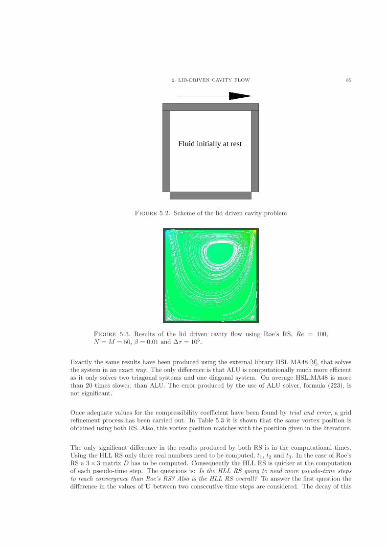
2. LID-DRIVEN CAVITY FLOW 85
������������������������
������������������������
Fluid initially at rest
Figure 5.2. Scheme of the lid driven cavity problem
Figure 5.3. Results of the lid driven cavity flow using Roe’s RS, Re = 100,N =M = 50, � = 0.01 and Δ� = 106.
Exactly the same results have been produced using the external library HSL MA48 [9], that solvesthe system in an exact way. The only difference is that ALU is computationally much more efficientas it only solves two triagonal systems and one diagonal system. On average HSL MA48 is morethan 20 times slower, than ALU. The error produced by the use of ALU solver, formula (223), isnot significant.
Once adequate values for the compressibility coefficient have been found by trial and error, a gridrefinement process has been carried out. In Table 5.3 it is shown that the same vortex position isobtained using both RS. Also, this vortex position matches with the position given in the literature.
The only significant difference in the results produced by both RS is in the computational times.Using the HLL RS only three real numbers need to be computed, t1, t2 and t3. In the case of Roe’sRS a 3× 3 matrix D has to be computed. Consequently the HLL RS is quicker at the computationof each pseudo-time step. The questions is: Is the HLL RS going to need more pseudo-time stepsto reach convergence than Roe’s RS? Also is the HLL RS overall? To answer the first question thedifference in the values of U between two consecutive time steps are considered. The decay of this
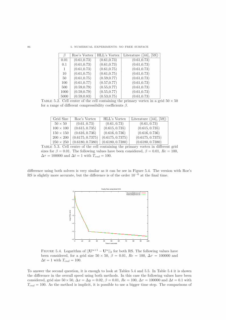
86 5. NUMERICAL EXPERIMENTS: NO FREE SURFACE
� Roe’s Vortex HLL’s Vortex Literature ([44], [59])0.01 (0.61,0.73) (0.61,0.73) (0.61,0.73)0.1 (0.61,0.73) (0.61,0.73) (0.61,0.73)1 (0.61,0.73) (0.61,0.75) (0.61,0.73)10 (0.61,0.75) (0.61,0.75) (0.61,0.73)50 (0.61,0.75) (0.59,0.77) (0.61,0.73)100 (0.61,0.77) (0.57,0.77) (0.61,0.73)500 (0.59,0.79) (0.55,0.77) (0.61,0.73)1000 (0.59,0.79) (0.55,0.77) (0.61,0.73)5000 (0.59,0.83) (0.53,0.75) (0.61,0.73)
Table 5.2. Cell center of the cell containing the primary vortex in a grid 50× 50for a range of different compressibility coefficients �.
Grid Size Roe’s Vortex HLL’s Vortex Literature ([44], [59])50× 50 (0.61, 0.73) (0.61, 0.73) (0.61, 0.73)100× 100 (0.615, 0.735) (0.615, 0.735) (0.615, 0.735)
150× 150 (0.616, 0.736) (0.616, 0.736) (0.616, 0.736)200× 200 (0.6175, 0.7375) (0.6175, 0.7375) (0.6175, 0.7375)250× 250 (0.6180, 0.7380) (0.6180, 0.7380) (0.6180, 0.7380)
Table 5.3. Cell centre of the cell containing the primary vortex in different gridsizes for � = 0.01. The following values have been considered, � = 0.01, Re = 100,Δ� = 100000 and Δt = 1 with Tend = 100.
difference using both solvers is very similar as it can be see in Figure 5.4. The version with Roe’sRS is slightly more accurate, but the difference is of the order 10−6 at the final time.
−6
−5
−4
−3
−2
−1
0
0 10 20 30 40 50 60 70 80 90 100
Log
of th
e er
ror
Time in seconds
Cavity flow using beta=0.01
HLLCavityErrors.txtRoeCavityErrors.txt
Figure 5.4. Logarithm of ∣∣Un+1 −Un∣∣2 for both RS. The following values havebeen considered, for a grid size 50 × 50, � = 0.01, Re = 100, Δ� = 100000 andΔt = 1 with Tend = 100.
To answer the second question, it is enough to look at Tables 5.4 and 5.5. In Table 5.4 it is shownthe difference in the overall speed using both methods. In this case the following values have beenconsidered, grid size 50×50, Δx = Δy = 0.02, � = 0.01, Re = 100, Δ� = 100000 and Δt = 0.1 withTend = 100. As the method is implicit, it is possible to use a bigger time step. The comparisons of
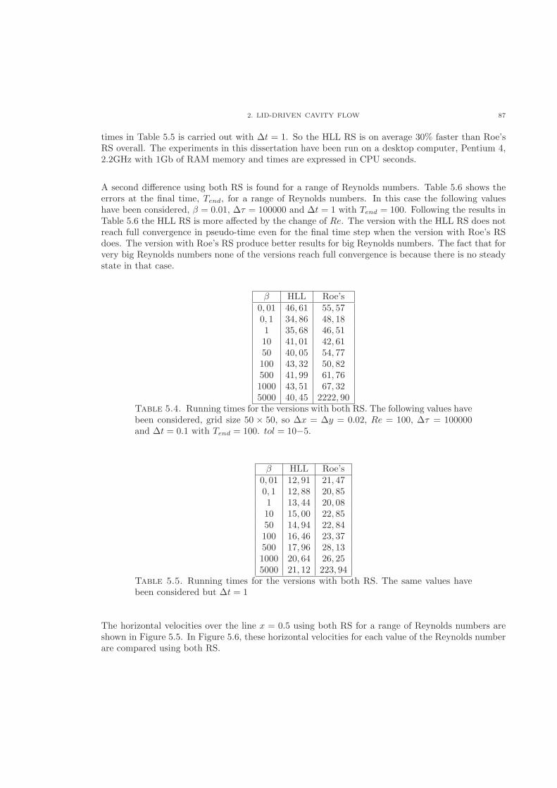
2. LID-DRIVEN CAVITY FLOW 87
times in Table 5.5 is carried out with Δt = 1. So the HLL RS is on average 30% faster than Roe’sRS overall. The experiments in this dissertation have been run on a desktop computer, Pentium 4,2.2GHz with 1Gb of RAM memory and times are expressed in CPU seconds.
A second difference using both RS is found for a range of Reynolds numbers. Table 5.6 shows theerrors at the final time, Tend, for a range of Reynolds numbers. In this case the following valueshave been considered, � = 0.01, Δ� = 100000 and Δt = 1 with Tend = 100. Following the results inTable 5.6 the HLL RS is more affected by the change of Re. The version with the HLL RS does notreach full convergence in pseudo-time even for the final time step when the version with Roe’s RSdoes. The version with Roe’s RS produce better results for big Reynolds numbers. The fact that forvery big Reynolds numbers none of the versions reach full convergence is because there is no steadystate in that case.
� HLL Roe’s0, 01 46, 61 55, 570, 1 34, 86 48, 181 35, 68 46, 5110 41, 01 42, 6150 40, 05 54, 77100 43, 32 50, 82500 41, 99 61, 761000 43, 51 67, 325000 40, 45 2222, 90
Table 5.4. Running times for the versions with both RS. The following values havebeen considered, grid size 50 × 50, so Δx = Δy = 0.02, Re = 100, Δ� = 100000and Δt = 0.1 with Tend = 100. tol = 10−5.
� HLL Roe’s0, 01 12, 91 21, 470, 1 12, 88 20, 851 13, 44 20, 0810 15, 00 22, 8550 14, 94 22, 84100 16, 46 23, 37500 17, 96 28, 131000 20, 64 26, 255000 21, 12 223, 94
Table 5.5. Running times for the versions with both RS. The same values havebeen considered but Δt = 1
The horizontal velocities over the line x = 0.5 using both RS for a range of Reynolds numbers areshown in Figure 5.5. In Figure 5.6, these horizontal velocities for each value of the Reynolds numberare compared using both RS.
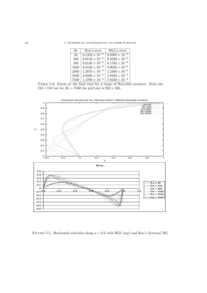
88 5. NUMERICAL EXPERIMENTS: NO FREE SURFACE
Re Roe’s error HLL’s error50 8.1250× 10⁻⁶ 9.0260× 10⁻⁶
100 9.9110× 10⁻⁶ 8.3520× 10⁻⁶
400 8.0140× 10⁻⁶ 8.1780× 10⁻⁶
1000 9.8120× 10⁻⁶ 9.9020× 10⁻⁶
2000 1.3870× 10⁻⁵ 1.2400× 10⁻⁵
5000 2.6890× 10⁻⁵ 1.8920× 10⁻³
7500 1.4790× 10⁻⁴ 7.8240× 10⁻⁴
Table 5.6. Errors at the final time for a range of Reynolds numbers. Grid size150× 150 but for Re = 7500 the grid size is 250× 250.
0
0.1
0.2
0.3
0.4
0.5
0.6
0.7
0.8
0.9
1
−0.4 −0.2 0 0.2 0.4 0.6 0.8 1
y
u
Horizontal velocities for HLL Riemann Solver. Different Reynolds numbers.
Re=50Re=100Re=400
Re=1000Re=2000Re=5000
Figure 5.5. Horizontal velocities along x = 0.5 with HLL (top) and Roe’s (bottom) RS.
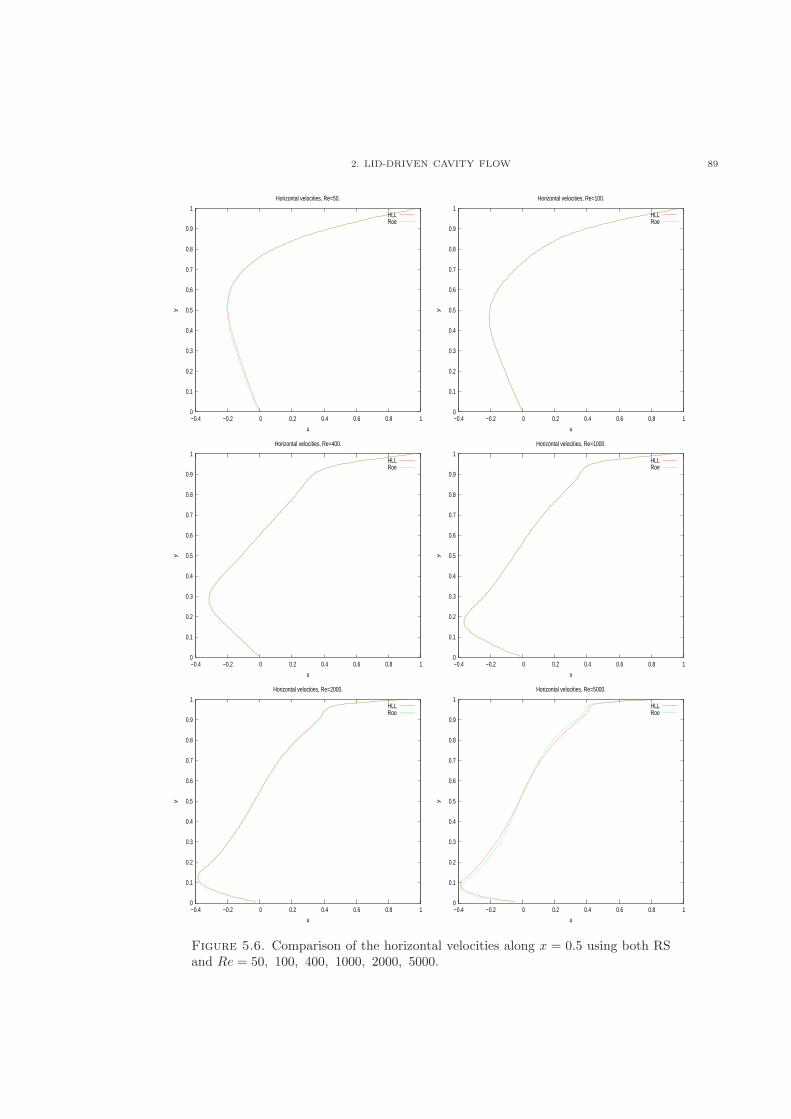
2. LID-DRIVEN CAVITY FLOW 89
0
0.1
0.2
0.3
0.4
0.5
0.6
0.7
0.8
0.9
1
−0.4 −0.2 0 0.2 0.4 0.6 0.8 1
y
u
Horizontal velocities, Re=50.
HLLRoe
0
0.1
0.2
0.3
0.4
0.5
0.6
0.7
0.8
0.9
1
−0.4 −0.2 0 0.2 0.4 0.6 0.8 1
y
u
Horizontal velocities, Re=100.
HLLRoe
0
0.1
0.2
0.3
0.4
0.5
0.6
0.7
0.8
0.9
1
−0.4 −0.2 0 0.2 0.4 0.6 0.8 1
y
u
Horizontal velocities, Re=400.
HLLRoe
0
0.1
0.2
0.3
0.4
0.5
0.6
0.7
0.8
0.9
1
−0.4 −0.2 0 0.2 0.4 0.6 0.8 1
y
u
Horizontal velocities, Re=1000.
HLLRoe
0
0.1
0.2
0.3
0.4
0.5
0.6
0.7
0.8
0.9
1
−0.4 −0.2 0 0.2 0.4 0.6 0.8 1
y
u
Horizontal velocities, Re=2000.
HLLRoe
0
0.1
0.2
0.3
0.4
0.5
0.6
0.7
0.8
0.9
1
−0.4 −0.2 0 0.2 0.4 0.6 0.8 1
y
u
Horizontal velocities, Re=5000.
HLLRoe
Figure 5.6. Comparison of the horizontal velocities along x = 0.5 using both RSand Re = 50, 100, 400, 1000, 2000, 5000.
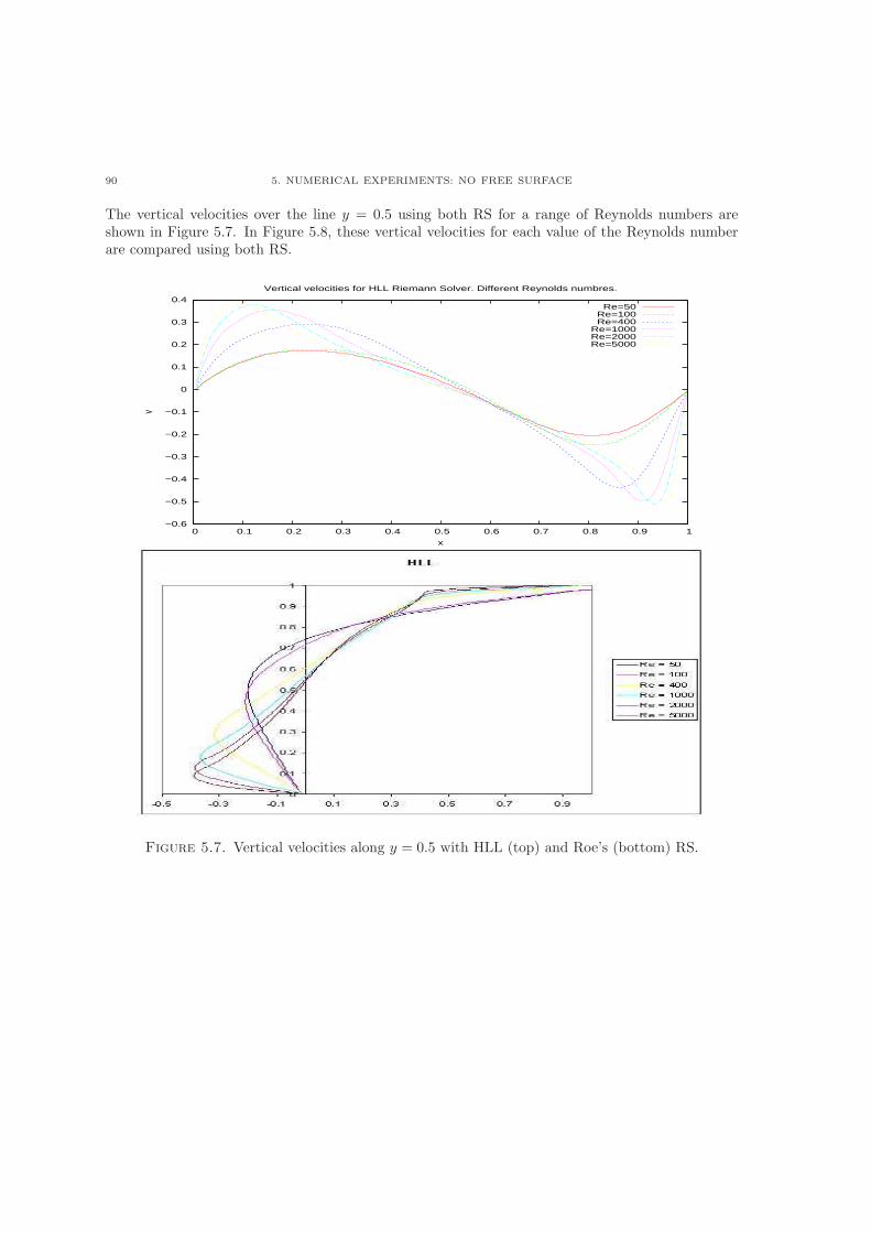
90 5. NUMERICAL EXPERIMENTS: NO FREE SURFACE
The vertical velocities over the line y = 0.5 using both RS for a range of Reynolds numbers areshown in Figure 5.7. In Figure 5.8, these vertical velocities for each value of the Reynolds numberare compared using both RS.
−0.6
−0.5
−0.4
−0.3
−0.2
−0.1
0
0.1
0.2
0.3
0.4
0 0.1 0.2 0.3 0.4 0.5 0.6 0.7 0.8 0.9 1
v
x
Vertical velocities for HLL Riemann Solver. Different Reynolds numbres.
Re=50Re=100Re=400
Re=1000Re=2000Re=5000
Figure 5.7. Vertical velocities along y = 0.5 with HLL (top) and Roe’s (bottom) RS.
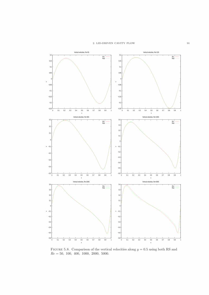
2. LID-DRIVEN CAVITY FLOW 91
−0.25
−0.2
−0.15
−0.1
−0.05
0
0.05
0.1
0.15
0.2
0 0.1 0.2 0.3 0.4 0.5 0.6 0.7 0.8 0.9 1
v
x
Vertical velocities, Re=50.
HLLRoe
−0.25
−0.2
−0.15
−0.1
−0.05
0
0.05
0.1
0.15
0.2
0 0.1 0.2 0.3 0.4 0.5 0.6 0.7 0.8 0.9 1
v
x
Vertical velocities, Re=100.
HLLRoe
−0.5
−0.4
−0.3
−0.2
−0.1
0
0.1
0.2
0.3
0 0.1 0.2 0.3 0.4 0.5 0.6 0.7 0.8 0.9 1
v
x
Vertical velocities, Re=400.
HLLRoe
−0.6
−0.5
−0.4
−0.3
−0.2
−0.1
0
0.1
0.2
0.3
0.4
0 0.1 0.2 0.3 0.4 0.5 0.6 0.7 0.8 0.9 1
v
x
Vertical velocities, Re=1000.
HLLRoe
−0.6
−0.5
−0.4
−0.3
−0.2
−0.1
0
0.1
0.2
0.3
0.4
0 0.1 0.2 0.3 0.4 0.5 0.6 0.7 0.8 0.9 1
v
x
Vertical velocities, Re=2000.
HLLRoe
−0.6
−0.5
−0.4
−0.3
−0.2
−0.1
0
0.1
0.2
0.3
0.4
0 0.1 0.2 0.3 0.4 0.5 0.6 0.7 0.8 0.9 1
v
x
Vertical velocities, Re=5000.
HLLRoe
Figure 5.8. Comparison of the vertical velocities along y = 0.5 using both RS andRe = 50, 100, 400, 1000, 2000, 5000.
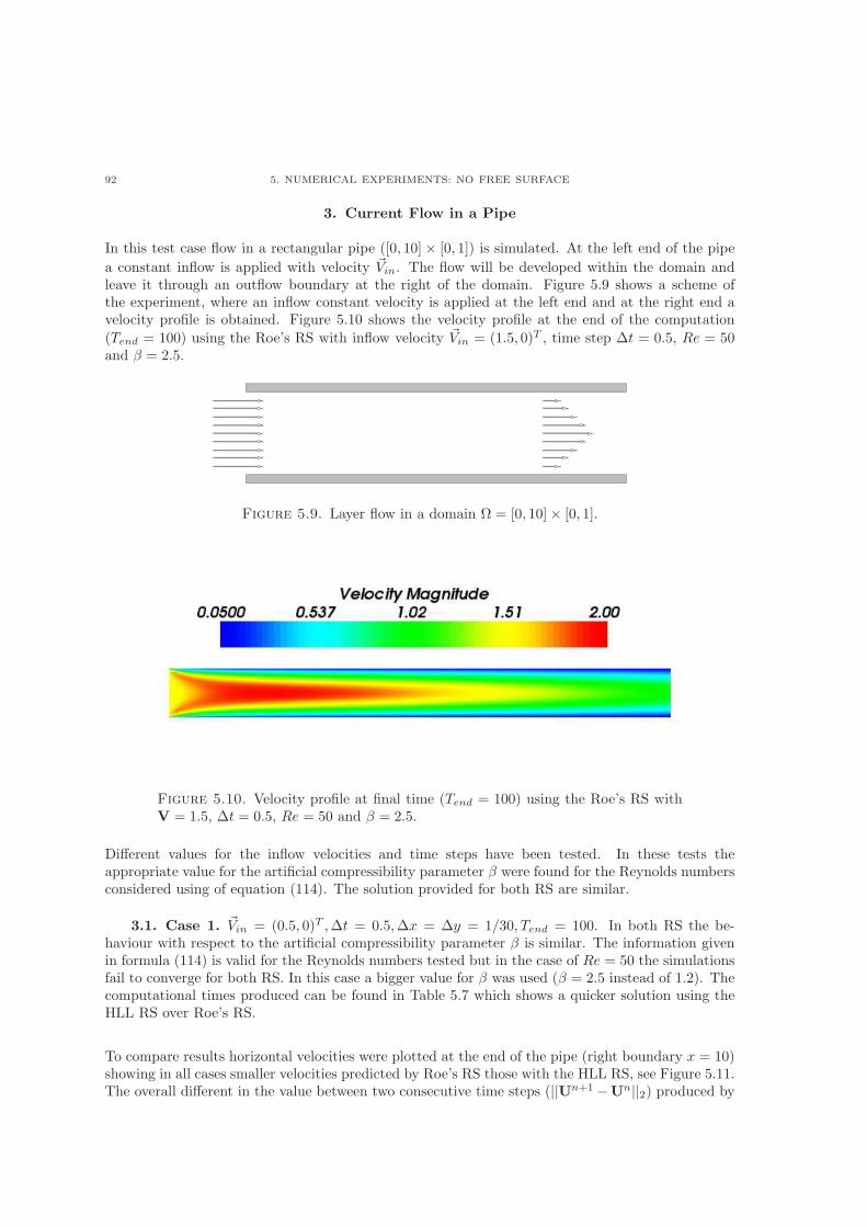
92 5. NUMERICAL EXPERIMENTS: NO FREE SURFACE
3. Current Flow in a Pipe
In this test case flow in a rectangular pipe ([0, 10] × [0, 1]) is simulated. At the left end of the pipe
a constant inflow is applied with velocity Vin. The flow will be developed within the domain andleave it through an outflow boundary at the right of the domain. Figure 5.9 shows a scheme ofthe experiment, where an inflow constant velocity is applied at the left end and at the right end avelocity profile is obtained. Figure 5.10 shows the velocity profile at the end of the computation
(Tend = 100) using the Roe’s RS with inflow velocity Vin = (1.5, 0)T , time step Δt = 0.5, Re = 50and � = 2.5.
Figure 5.9. Layer flow in a domain Ω = [0, 10]× [0, 1].
Figure 5.10. Velocity profile at final time (Tend = 100) using the Roe’s RS withV = 1.5, Δt = 0.5, Re = 50 and � = 2.5.
Different values for the inflow velocities and time steps have been tested. In these tests theappropriate value for the artificial compressibility parameter � were found for the Reynolds numbersconsidered using of equation (114). The solution provided for both RS are similar.
3.1. Case 1. Vin = (0.5, 0)T ,Δt = 0.5,Δx = Δy = 1/30, Tend = 100. In both RS the be-haviour with respect to the artificial compressibility parameter � is similar. The information givenin formula (114) is valid for the Reynolds numbers tested but in the case of Re = 50 the simulationsfail to converge for both RS. In this case a bigger value for � was used (� = 2.5 instead of 1.2). Thecomputational times produced can be found in Table 5.7 which shows a quicker solution using theHLL RS over Roe’s RS.
To compare results horizontal velocities were plotted at the end of the pipe (right boundary x = 10)showing in all cases smaller velocities predicted by Roe’s RS those with the HLL RS, see Figure 5.11.The overall different in the value between two consecutive time steps (∣∣Un+1 −Un∣∣2) produced by
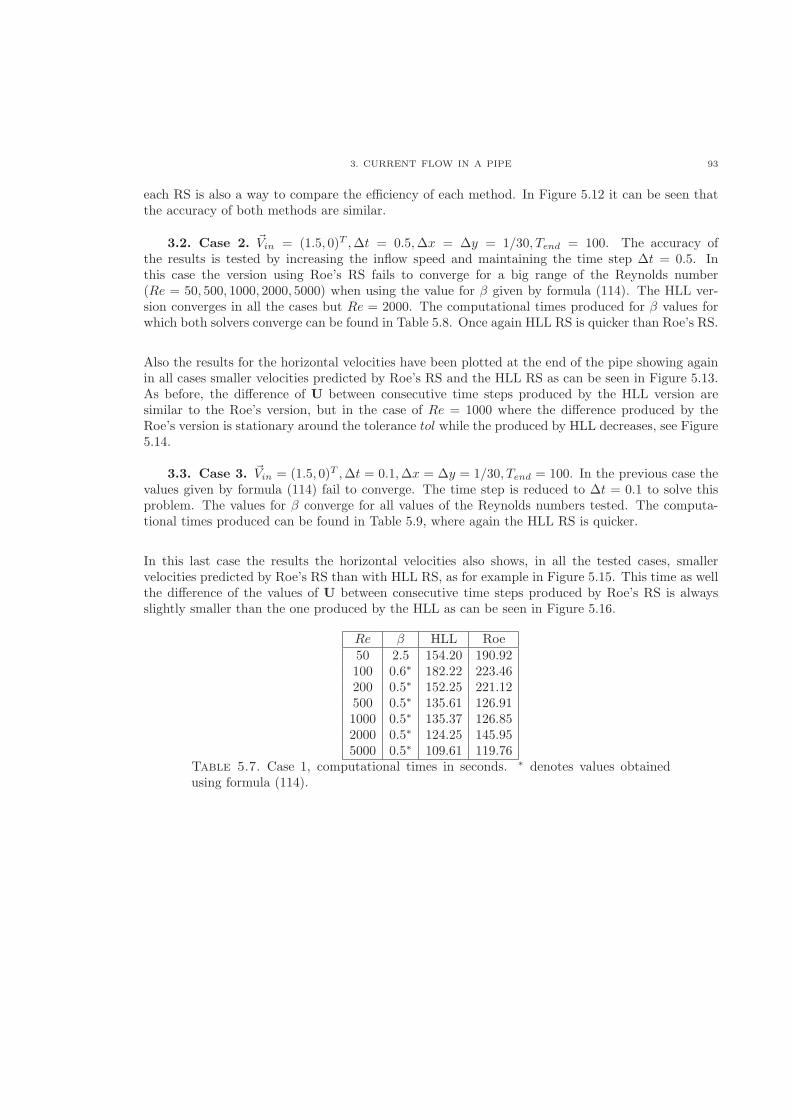
3. CURRENT FLOW IN A PIPE 93
each RS is also a way to compare the efficiency of each method. In Figure 5.12 it can be seen thatthe accuracy of both methods are similar.
3.2. Case 2. Vin = (1.5, 0)T ,Δt = 0.5,Δx = Δy = 1/30, Tend = 100. The accuracy ofthe results is tested by increasing the inflow speed and maintaining the time step Δt = 0.5. Inthis case the version using Roe’s RS fails to converge for a big range of the Reynolds number(Re = 50, 500, 1000, 2000, 5000) when using the value for � given by formula (114). The HLL ver-sion converges in all the cases but Re = 2000. The computational times produced for � values forwhich both solvers converge can be found in Table 5.8. Once again HLL RS is quicker than Roe’s RS.
Also the results for the horizontal velocities have been plotted at the end of the pipe showing againin all cases smaller velocities predicted by Roe’s RS and the HLL RS as can be seen in Figure 5.13.As before, the difference of U between consecutive time steps produced by the HLL version aresimilar to the Roe’s version, but in the case of Re = 1000 where the difference produced by theRoe’s version is stationary around the tolerance tol while the produced by HLL decreases, see Figure5.14.
3.3. Case 3. Vin = (1.5, 0)T ,Δt = 0.1,Δx = Δy = 1/30, Tend = 100. In the previous case thevalues given by formula (114) fail to converge. The time step is reduced to Δt = 0.1 to solve thisproblem. The values for � converge for all values of the Reynolds numbers tested. The computa-tional times produced can be found in Table 5.9, where again the HLL RS is quicker.
In this last case the results the horizontal velocities also shows, in all the tested cases, smallervelocities predicted by Roe’s RS than with HLL RS, as for example in Figure 5.15. This time as wellthe difference of the values of U between consecutive time steps produced by Roe’s RS is alwaysslightly smaller than the one produced by the HLL as can be seen in Figure 5.16.
Re � HLL Roe50 2.5 154.20 190.92100 0.6∗ 182.22 223.46200 0.5∗ 152.25 221.12500 0.5∗ 135.61 126.911000 0.5∗ 135.37 126.852000 0.5∗ 124.25 145.955000 0.5∗ 109.61 119.76
Table 5.7. Case 1, computational times in seconds. ∗ denotes values obtainedusing formula (114).
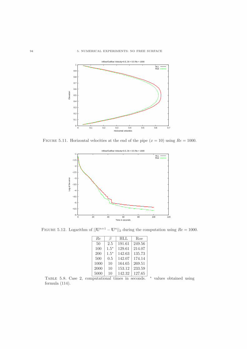
94 5. NUMERICAL EXPERIMENTS: NO FREE SURFACE
0
0.1
0.2
0.3
0.4
0.5
0.6
0.7
0.8
0.9
1
0 0.1 0.2 0.3 0.4 0.5 0.6 0.7
Ele
vatio
n
Horizontal velocities
Inflow/Outflow Velocity=0.5, Dt = 0.5 Re = 1000
HLLRoe
Figure 5.11. Horizontal velocities at the end of the pipe (x = 10) using Re = 1000.
−6
−5.5
−5
−4.5
−4
−3.5
−3
−2.5
−2
−1.5
−1
0 20 40 60 80 100 120
Log
of th
e er
ror
Time in seconds
Inflow/Outflow Velocity=0.5, Dt = 0.5 Re = 1000
HLLRoe
Figure 5.12. Logarithm of ∣∣Un+1 −Un∣∣2 during the computation using Re = 1000.
Re � HLL Roe50 2.5 191.61 249.56100 1.5∗ 129.61 214.07200 1.5∗ 142.63 135.73500 0.5 142.07 174.141000 10 164.65 269.512000 10 153.12 233.595000 10 142.32 127.65
Table 5.8. Case 2, computational times in seconds. ∗ values obtained usingformula (114).
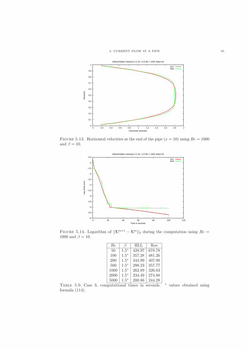
3. CURRENT FLOW IN A PIPE 95
0
0.1
0.2
0.3
0.4
0.5
0.6
0.7
0.8
0.9
1
0 0.2 0.4 0.6 0.8 1 1.2 1.4 1.6 1.8 2
Ele
vatio
n
Horizontal velocities
Inflow/Outflow Velocity=1.5, Dt = 0.5 Re = 1000, Beta=10
HLLRoe
Figure 5.13. Horizontal velocities at the end of the pipe (x = 10) using Re = 1000and � = 10.
−6
−5.5
−5
−4.5
−4
−3.5
−3
−2.5
−2
−1.5
−1
−0.5
0 20 40 60 80 100 120
Log
of th
e er
ror
Time in seconds
Inflow/Outflow Velocity=1.5, Dt = 0.5 Re = 1000, Beta=10
HLLRoe
Figure 5.14. Logarithm of ∣∣Un+1 − Un∣∣2 during the computation using Re =1000 and � = 10.
Re � HLL Roe50 1.5∗ 428.97 678.78100 1.5∗ 357.28 481.26200 1.5∗ 344.99 407.90500 1.5∗ 298.23 357.771000 1.5∗ 262.89 326.032000 1.5∗ 234.49 274.885000 1.5∗ 200.86 244.28
Table 5.9. Case 3, computational times in seconds. ∗ values obtained usingformula (114).
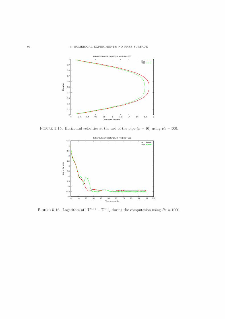
96 5. NUMERICAL EXPERIMENTS: NO FREE SURFACE
0
0.1
0.2
0.3
0.4
0.5
0.6
0.7
0.8
0.9
1
0 0.2 0.4 0.6 0.8 1 1.2 1.4 1.6 1.8 2
Ele
vatio
n
Horizontal velocities
Inflow/Outflow Velocity=1.5, Dt = 0.1 Re = 500
HLLRoe
Figure 5.15. Horizontal velocities at the end of the pipe (x = 10) using Re = 500.
−6
−5.5
−5
−4.5
−4
−3.5
−3
−2.5
−2
−1.5
−1
−0.5
0 10 20 30 40 50 60 70 80 90 100 110
Log
of th
e er
ror
Time in seconds
Inflow/Outflow Velocity=1.5, Dt = 0.1 Re = 500
HLLRoe
Figure 5.16. Logarithm of ∣∣Un+1 −Un∣∣2 during the computation using Re = 1000.
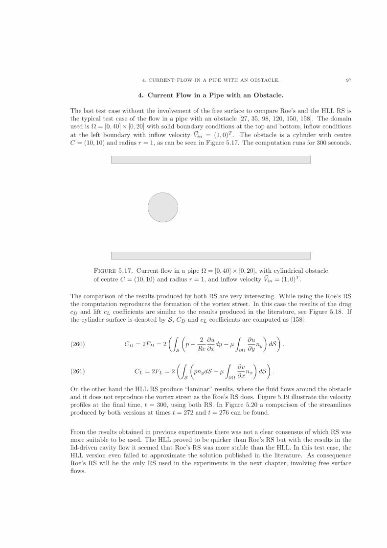
4. CURRENT FLOW IN A PIPE WITH AN OBSTACLE. 97
4. Current Flow in a Pipe with an Obstacle.
The last test case without the involvement of the free surface to compare Roe’s and the HLL RS isthe typical test case of the flow in a pipe with an obstacle [27, 35, 98, 120, 150, 158]. The domainused is Ω = [0, 40]× [0, 20] with solid boundary conditions at the top and bottom, inflow conditions
at the left boundary with inflow velocity Vin = (1, 0)T . The obstacle is a cylinder with centreC = (10, 10) and radius r = 1, as can be seen in Figure 5.17. The computation runs for 300 seconds.
Figure 5.17. Current flow in a pipe Ω = [0, 40]× [0, 20], with cylindrical obstacle
of centre C = (10, 10) and radius r = 1, and inflow velocity Vin = (1, 0)T .
The comparison of the results produced by both RS are very interesting. While using the Roe’s RSthe computation reproduces the formation of the vortex street. In this case the results of the dragcD and lift cL coefficients are similar to the results produced in the literature, see Figure 5.18. Ifthe cylinder surface is denoted by S, CD and cL coefficients are computed as [158]:
CD = 2FD = 2
(∫
S
(
p− 2
Re
∂u
∂xdy − �
∫
∂Ω
∂u
∂yny
)
dS)
.(260)
CL = 2FL = 2
(∫
S
(
pnydS − �
∫
∂Ω
∂v
∂xnx
)
dS)
.(261)
On the other hand the HLL RS produce “laminar” results, where the fluid flows around the obstacleand it does not reproduce the vortex street as the Roe’s RS does. Figure 5.19 illustrate the velocityprofiles at the final time, t = 300, using both RS. In Figure 5.20 a comparison of the streamlinesproduced by both versions at times t = 272 and t = 276 can be found.
From the results obtained in previous experiments there was not a clear consensus of which RS wasmore suitable to be used. The HLL proved to be quicker than Roe’s RS but with the results in thelid-driven cavity flow it seemed that Roe’s RS was more stable than the HLL. In this test case, theHLL version even failed to approximate the solution published in the literature. As consequenceRoe’s RS will be the only RS used in the experiments in the next chapter, involving free surfaceflows.
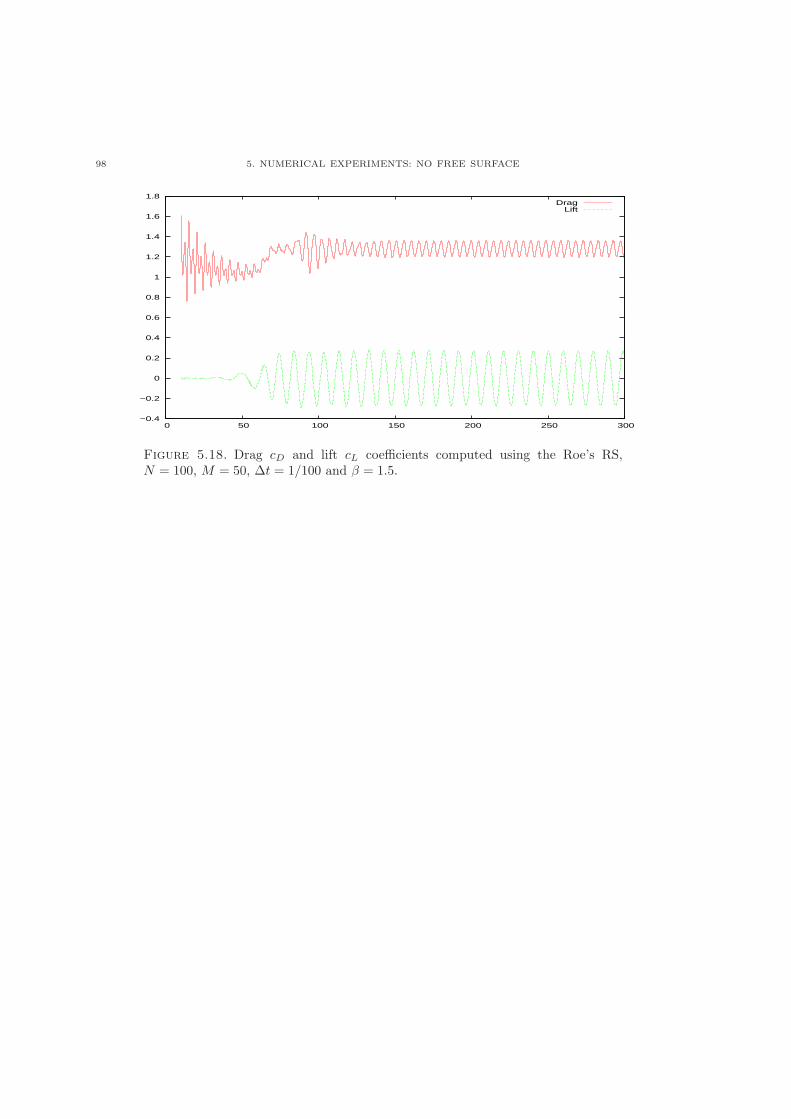
98 5. NUMERICAL EXPERIMENTS: NO FREE SURFACE
−0.4
−0.2
0
0.2
0.4
0.6
0.8
1
1.2
1.4
1.6
1.8
0 50 100 150 200 250 300
DragLift
Figure 5.18. Drag cD and lift cL coefficients computed using the Roe’s RS,N = 100, M = 50, Δt = 1/100 and � = 1.5.
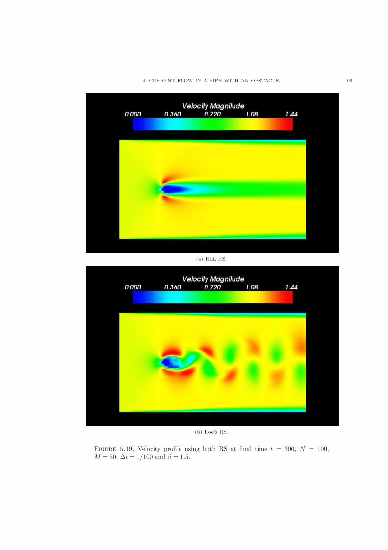
4. CURRENT FLOW IN A PIPE WITH AN OBSTACLE. 99
(a) HLL RS.
(b) Roe’s RS.
Figure 5.19. Velocity profile using both RS at final time t = 300, N = 100,M = 50, Δt = 1/100 and � = 1.5.
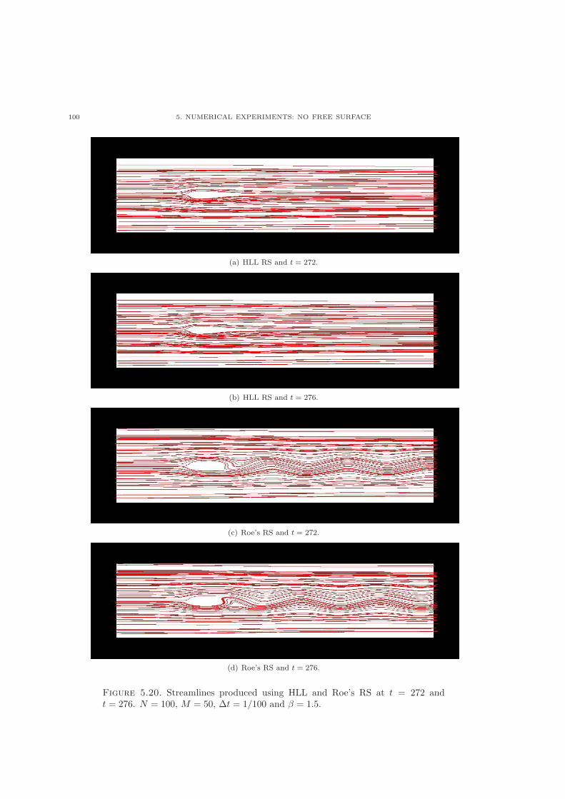
100 5. NUMERICAL EXPERIMENTS: NO FREE SURFACE
(a) HLL RS and t = 272.
(b) HLL RS and t = 276.
(c) Roe’s RS and t = 272.
(d) Roe’s RS and t = 276.
Figure 5.20. Streamlines produced using HLL and Roe’s RS at t = 272 andt = 276. N = 100, M = 50, Δt = 1/100 and � = 1.5.
CHAPTER 6
Numerical Experiments: Free Surface
Numerical experiments in the presence of free surfaces are presented in this chapter. The com-putational domain is unknown a priori, as the position at the next time step is located using thevelocities computed at the previous time step. The capabilities of the CCCM are tested in thecase of the free surface, with the restrictions already known (see Figures 2.2 and 2.13). In thisset of experiments only the Roe’s RS is used as it has been more reliable. The dependency of theresults of the experiments on the artificial compressibility parameter � will be studied in this chapter.
The first experiment that have been studied is, as before, to leave the flow unperturbed (flat freesurface as initial condition) and see the evolution, this experiment will highlight possible errors in thesolver. In all the tested configuration of flows it remained undisturbed and therefore the experimentwas successful.
The numerical experiments of the inviscid and viscous sloshing tank, mass generated waves, semi-dam break and current flow passing a bump (CFPOB) and a cylindrical hydrofoil (CFPCBF) arestudied. To introduce the CCCM to ship generated waves the last numerical experiment consist ofa cylinder placed at the free surface in a current flow (CFPCFS).
1. Small Amplitude Sloshing Tank
1.1. Inviscid. This classical test case has been studied using different configurations by variousauthors [12, 27, 117, 149]. The numerical experiment consist in a fluid in a tank with solid boundaryconditions. The fluid is initially at rest with a sinusoidal free surface, see Figure 6.1. The geometryof the tank in this work is Ω = [0, 1]× [0, 1.1], the average depth is d = 1, the amplitude is A = 0.1and L is the length of the tank (L = 1). The initial elevation of the free surface is given by,
(262) ℎ(x) = d+A cos(x�/L).
The solution of this numerical experiment should be an wave oscillating at a constant period withoutany loss of amplitude, as it can be seen in the articles mentioned above. For inviscid flows thereis no formula providing a “recommended” value for �, unlike the viscous case where Nithiarasu’sequation (114) gives this “recommendation”. The appropriate value for � has to be found in a testand trial procedure. In the results obtained in the present work there is loss of amplitude and changeof period for all the tested values of the artificial compressibility parameter, � (0.01− 500000), seeFigures 6.2 and 6.3. Neither is there information about the best selection of the time step, equation(116), therefore different values have been used Δt = 1/20, 1/100, 1/500. These changes in thetime steps used shows that the damping of the amplitude is smaller with smaller time steps, theperiod also is slightly smaller when using smaller time steps, see Figures 6.4, 6.5, 6.6, 6.7. It canbe observed in the mentioned Figures that very big values of � breaks the regularity of the wavesand that small times steps produce instabilities in the results. The grid resolution also has a small
101
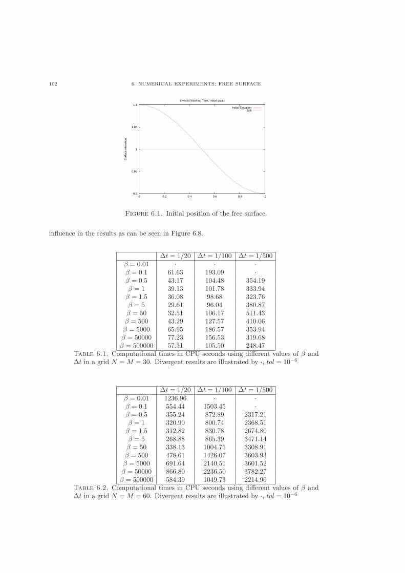
102 6. NUMERICAL EXPERIMENTS: FREE SURFACE
0.9
0.95
1
1.05
1.1
0 0.2 0.4 0.6 0.8 1
Sur
face
ele
vatio
n
Inviscid Sloshing Tank. Initial data.
Initial ElevationStill
Figure 6.1. Initial position of the free surface.
influence in the results as can be seen in Figure 6.8.
Δt = 1/20 Δt = 1/100 Δt = 1/500� = 0.01 ⋅ ⋅ ⋅� = 0.1 61.63 193.09 ⋅� = 0.5 43.17 104.48 354.19� = 1 39.13 101.78 333.94� = 1.5 36.08 98.68 323.76� = 5 29.61 96.04 380.87� = 50 32.51 106.17 511.43� = 500 43.29 127.57 410.06� = 5000 65.95 186.57 353.94� = 50000 77.23 156.53 319.68� = 500000 57.31 105.50 248.47
Table 6.1. Computational times in CPU seconds using different values of � andΔt in a grid N =M = 30. Divergent results are illustrated by ⋅, tol = 10−6
Δt = 1/20 Δt = 1/100 Δt = 1/500� = 0.01 1236.96 ⋅ ⋅� = 0.1 554.44 1503.45 ⋅� = 0.5 355.24 872.89 2317.21� = 1 320.90 800.74 2368.51� = 1.5 312.82 830.78 2674.80� = 5 268.88 865.39 3471.14� = 50 338.13 1004.75 3308.91� = 500 478.61 1426.07 3603.93� = 5000 691.64 2140.51 3601.52� = 50000 866.80 2236.50 3782.27� = 500000 584.39 1049.73 2214.90
Table 6.2. Computational times in CPU seconds using different values of � andΔt in a grid N =M = 60. Divergent results are illustrated by ⋅, tol = 10−6
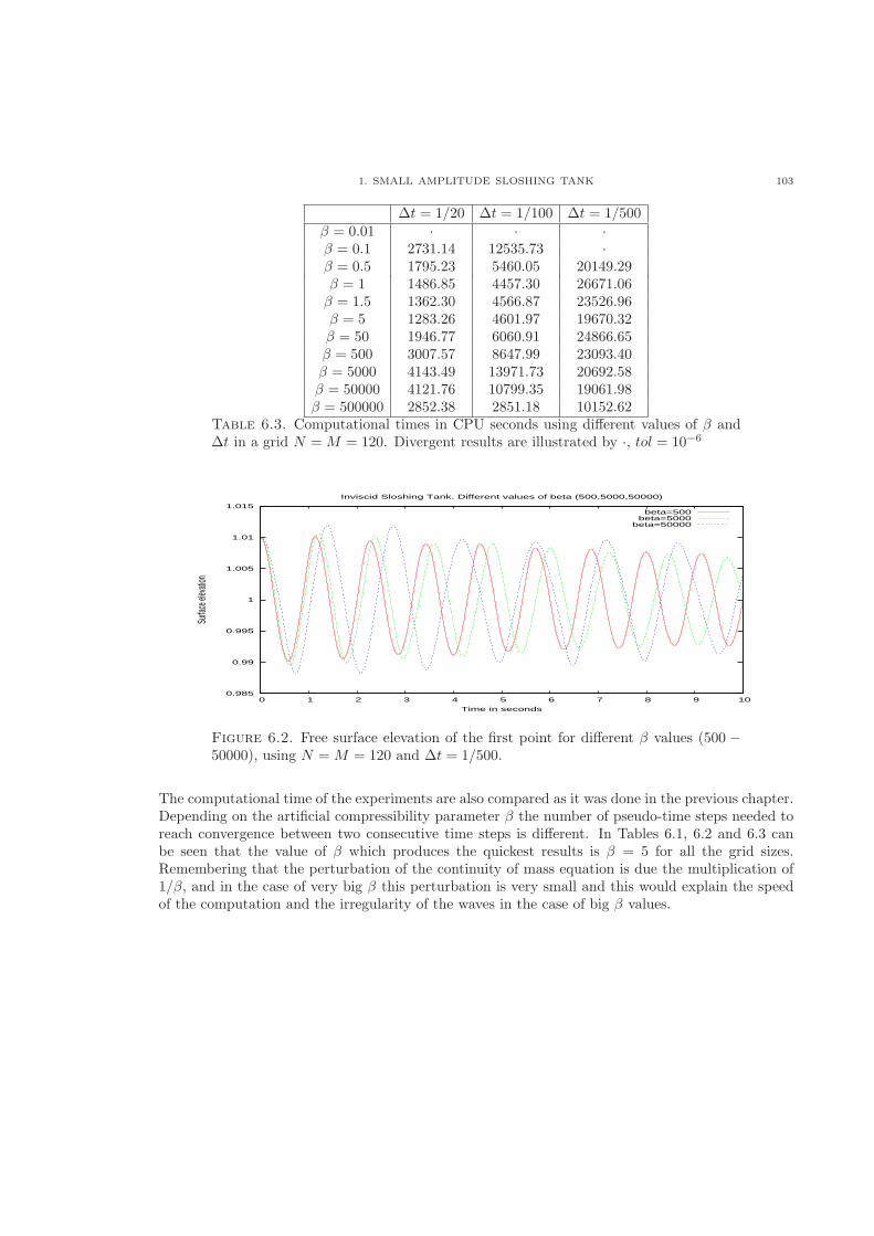
1. SMALL AMPLITUDE SLOSHING TANK 103
Δt = 1/20 Δt = 1/100 Δt = 1/500� = 0.01 ⋅ ⋅ ⋅� = 0.1 2731.14 12535.73 ⋅� = 0.5 1795.23 5460.05 20149.29� = 1 1486.85 4457.30 26671.06� = 1.5 1362.30 4566.87 23526.96� = 5 1283.26 4601.97 19670.32� = 50 1946.77 6060.91 24866.65� = 500 3007.57 8647.99 23093.40� = 5000 4143.49 13971.73 20692.58� = 50000 4121.76 10799.35 19061.98� = 500000 2852.38 2851.18 10152.62
Table 6.3. Computational times in CPU seconds using different values of � andΔt in a grid N =M = 120. Divergent results are illustrated by ⋅, tol = 10−6
0.985
0.99
0.995
1
1.005
1.01
1.015
0 1 2 3 4 5 6 7 8 9 10
Surfa
ce el
evati
on
Time in seconds
Inviscid Sloshing Tank. Different values of beta (500,5000,50000)
beta=500beta=5000
beta=50000
Figure 6.2. Free surface elevation of the first point for different � values (500 −50000), using N =M = 120 and Δt = 1/500.
The computational time of the experiments are also compared as it was done in the previous chapter.Depending on the artificial compressibility parameter � the number of pseudo-time steps needed toreach convergence between two consecutive time steps is different. In Tables 6.1, 6.2 and 6.3 canbe seen that the value of � which produces the quickest results is � = 5 for all the grid sizes.Remembering that the perturbation of the continuity of mass equation is due the multiplication of1/�, and in the case of very big � this perturbation is very small and this would explain the speedof the computation and the irregularity of the waves in the case of big � values.
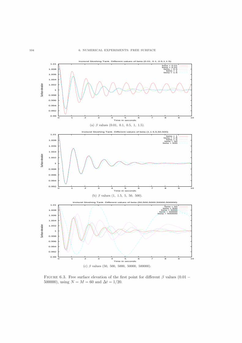
104 6. NUMERICAL EXPERIMENTS: FREE SURFACE
0.99
0.992
0.994
0.996
0.998
1
1.002
1.004
1.006
1.008
1.01
0 1 2 3 4 5 6 7 8 9 10
Surfa
ce el
evati
on
Time in seconds
Inviscid Sloshing Tank. Different values of beta (0.01, 0.1, 0.5,1,1.5)
beta = 0.01beta = 0.01
beta = 0.5beta = 1
beta = 1.5
(a) � values (0.01, 0.1, 0.5, 1, 1.5).
0.992
0.994
0.996
0.998
1
1.002
1.004
1.006
1.008
1.01
0 1 2 3 4 5 6 7 8 9 10
Surfa
ce el
evati
on
Time in seconds
Inviscid Sloshing Tank. Different values of beta (1,1.5,5,50,500)
beta = 1beta = 1.5
beta = 5beta = 50
beta = 500
(b) � values (1, 1.5, 5, 50, 500).
0.99
0.992
0.994
0.996
0.998
1
1.002
1.004
1.006
1.008
1.01
0 1 2 3 4 5 6 7 8 9 10
Surfa
ce el
evati
on
Time in seconds
Inviscid Sloshing Tank. Different values of beta (50,500,5000,50000,500000)
beta = 50beta = 500
beta = 5000beta = 50000
beta = 500000
(c) � values (50, 500, 5000, 50000, 500000).
Figure 6.3. Free surface elevation of the first point for different � values (0.01 −500000), using N =M = 60 and Δt = 1/20.
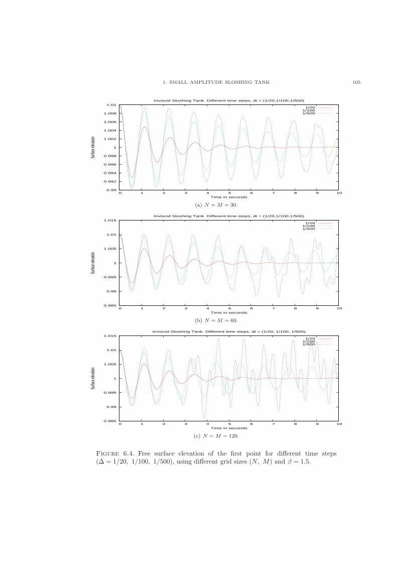
1. SMALL AMPLITUDE SLOSHING TANK 105
0.99
0.992
0.994
0.996
0.998
1
1.002
1.004
1.006
1.008
1.01
0 1 2 3 4 5 6 7 8 9 10
Surfa
ce el
evati
on
Time in seconds
Inviscid Sloshing Tank. Different time steps, dt = (1/20,1/100,1/500)
1/201/1001/500
(a) N = M = 30.
0.985
0.99
0.995
1
1.005
1.01
1.015
0 1 2 3 4 5 6 7 8 9 10
Surfa
ce el
evati
on
Time in seconds
Inviscid Sloshing Tank. Different time steps, dt = (1/20,1/100,1/500)
1/201/1001/500
(b) N = M = 60.
0.985
0.99
0.995
1
1.005
1.01
1.015
0 1 2 3 4 5 6 7 8 9 10
Surfa
ce el
evati
on
Time in seconds
Inviscid Sloshing Tank. Different time steps, dt = (1/20, 1/100, 1/500)
1/201/1001/500
(c) N = M = 120.
Figure 6.4. Free surface elevation of the first point for different time steps(Δ = 1/20, 1/100, 1/500), using different grid sizes (N, M) and � = 1.5.
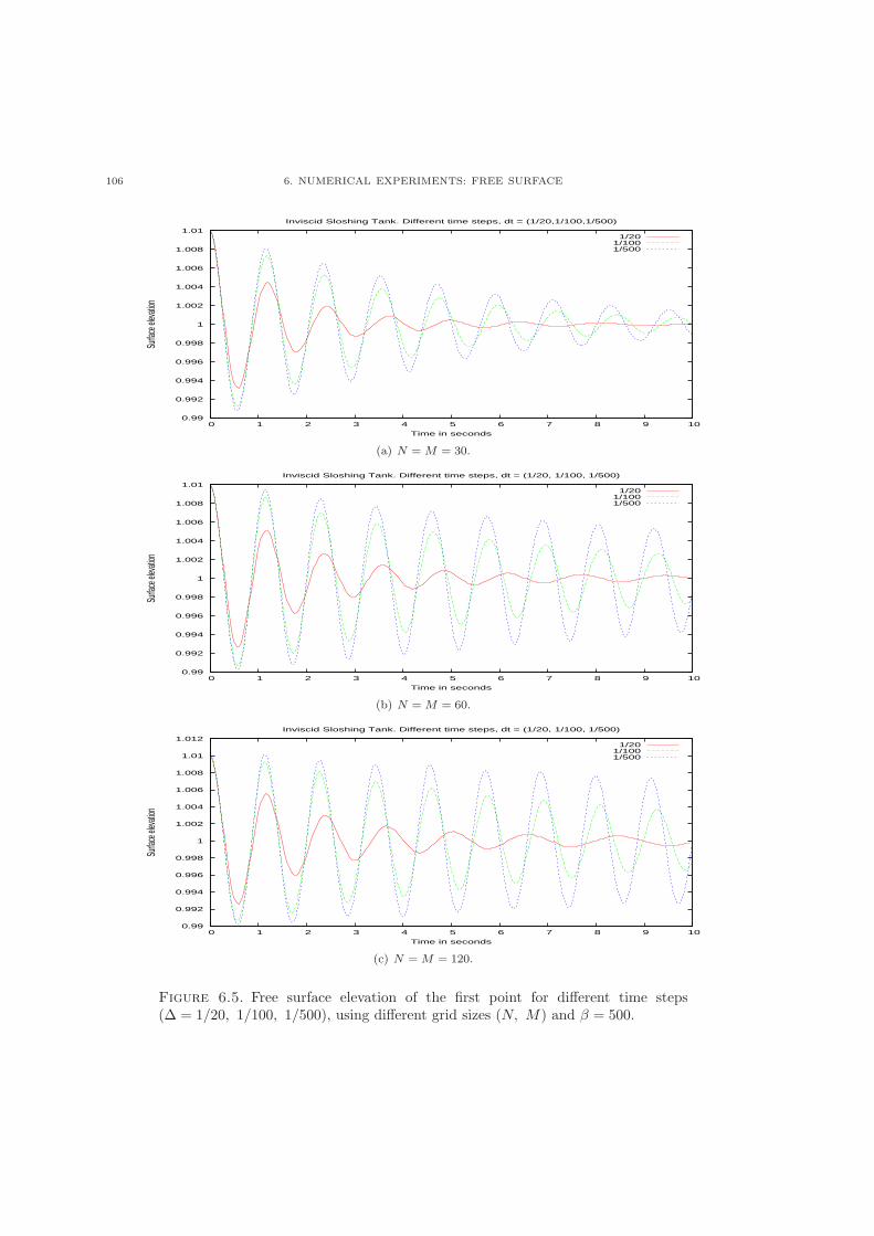
106 6. NUMERICAL EXPERIMENTS: FREE SURFACE
0.99
0.992
0.994
0.996
0.998
1
1.002
1.004
1.006
1.008
1.01
0 1 2 3 4 5 6 7 8 9 10
Surfa
ce el
evati
on
Time in seconds
Inviscid Sloshing Tank. Different time steps, dt = (1/20,1/100,1/500)
1/201/1001/500
(a) N = M = 30.
0.99
0.992
0.994
0.996
0.998
1
1.002
1.004
1.006
1.008
1.01
0 1 2 3 4 5 6 7 8 9 10
Surfa
ce el
evati
on
Time in seconds
Inviscid Sloshing Tank. Different time steps, dt = (1/20, 1/100, 1/500)
1/201/1001/500
(b) N = M = 60.
0.99
0.992
0.994
0.996
0.998
1
1.002
1.004
1.006
1.008
1.01
1.012
0 1 2 3 4 5 6 7 8 9 10
Surfa
ce el
evati
on
Time in seconds
Inviscid Sloshing Tank. Different time steps, dt = (1/20, 1/100, 1/500)
1/201/1001/500
(c) N = M = 120.
Figure 6.5. Free surface elevation of the first point for different time steps(Δ = 1/20, 1/100, 1/500), using different grid sizes (N, M) and � = 500.
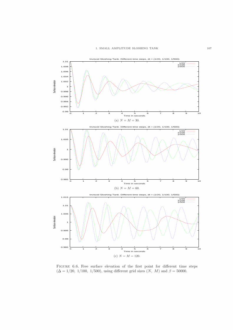
1. SMALL AMPLITUDE SLOSHING TANK 107
0.99
0.992
0.994
0.996
0.998
1
1.002
1.004
1.006
1.008
1.01
0 1 2 3 4 5 6 7 8 9 10
Surfa
ce el
evati
on
Time in seconds
Inviscid Sloshing Tank. Different time steps, dt = (1/20, 1/100, 1/500)
1/201/1001/500
(a) N = M = 30.
0.985
0.99
0.995
1
1.005
1.01
0 1 2 3 4 5 6 7 8 9 10
Surfa
ce el
evati
on
Time in seconds
Inviscid Sloshing Tank. Different time steps, dt = (1/20, 1/100, 1/500)
1/201/1001/500
(b) N = M = 60.
0.985
0.99
0.995
1
1.005
1.01
1.015
0 1 2 3 4 5 6 7 8 9 10
Surfa
ce el
evati
on
Time in seconds
Inviscid Sloshing Tank. Different time steps, dt = (1/20, 1/100, 1/500)
1/201/1001/500
(c) N = M = 120.
Figure 6.6. Free surface elevation of the first point for different time steps(Δ = 1/20, 1/100, 1/500), using different grid sizes (N, M) and � = 50000.

108 6. NUMERICAL EXPERIMENTS: FREE SURFACE
0.99
0.992
0.994
0.996
0.998
1
1.002
1.004
1.006
1.008
1.01
0 1 2 3 4 5 6 7 8 9 10
Surfa
ce el
evati
on
Time in seconds
Inviscid Sloshing Tank. Different time steps, dt = (1/20, 1/100, 1/500)
1/201/1001/500
(a) N = M = 30.
0.985
0.99
0.995
1
1.005
1.01
1.015
0 1 2 3 4 5 6 7 8 9 10
Surfa
ce el
evati
on
Time in seconds
Inviscid Sloshing Tank. Different time steps, dt = (1/20, 1/100, 1/500)
1/201/1001/500
(b) N = M = 60.
0.98
0.985
0.99
0.995
1
1.005
1.01
1.015
1.02
1.025
0 1 2 3 4 5 6 7 8 9 10
Surfa
ce el
evati
on
Time in seconds
Inviscid Sloshing Tank. Different time steps, dt = (1/20, 1/100, 1/500)
1/201/1001/500
(c) N = M = 120.
Figure 6.7. Free surface elevation of the first point for different time steps(Δ = 1/20, 1/100, 1/500), using different grid sizes (N, M) and � = 500000.
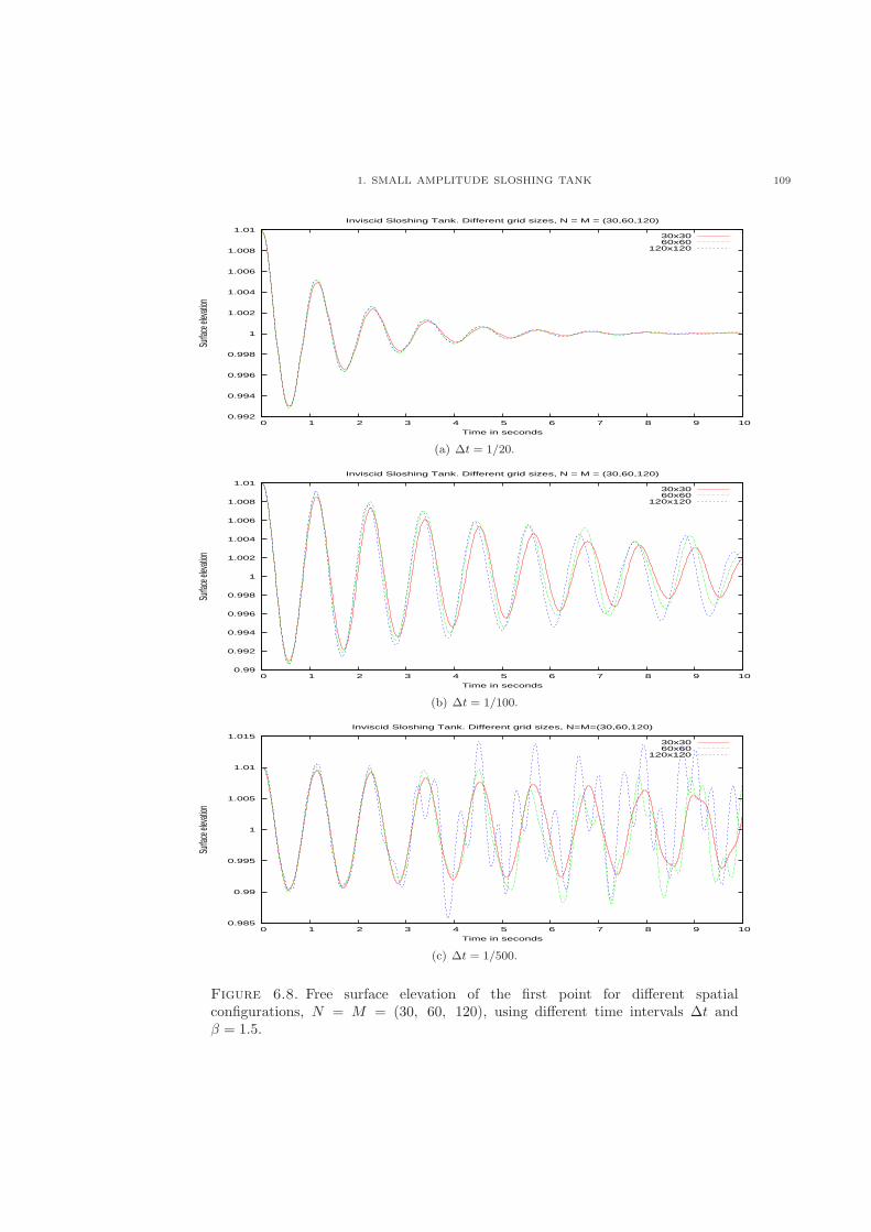
1. SMALL AMPLITUDE SLOSHING TANK 109
0.992
0.994
0.996
0.998
1
1.002
1.004
1.006
1.008
1.01
0 1 2 3 4 5 6 7 8 9 10
Surfa
ce el
evati
on
Time in seconds
Inviscid Sloshing Tank. Different grid sizes, N = M = (30,60,120)
30x3060x60
120x120
(a) Δt = 1/20.
0.99
0.992
0.994
0.996
0.998
1
1.002
1.004
1.006
1.008
1.01
0 1 2 3 4 5 6 7 8 9 10
Surfa
ce el
evati
on
Time in seconds
Inviscid Sloshing Tank. Different grid sizes, N = M = (30,60,120)
30x3060x60
120x120
(b) Δt = 1/100.
0.985
0.99
0.995
1
1.005
1.01
1.015
0 1 2 3 4 5 6 7 8 9 10
Surfa
ce el
evati
on
Time in seconds
Inviscid Sloshing Tank. Different grid sizes, N=M=(30,60,120)
30x3060x60
120x120
(c) Δt = 1/500.
Figure 6.8. Free surface elevation of the first point for different spatialconfigurations, N = M = (30, 60, 120), using different time intervals Δt and� = 1.5.
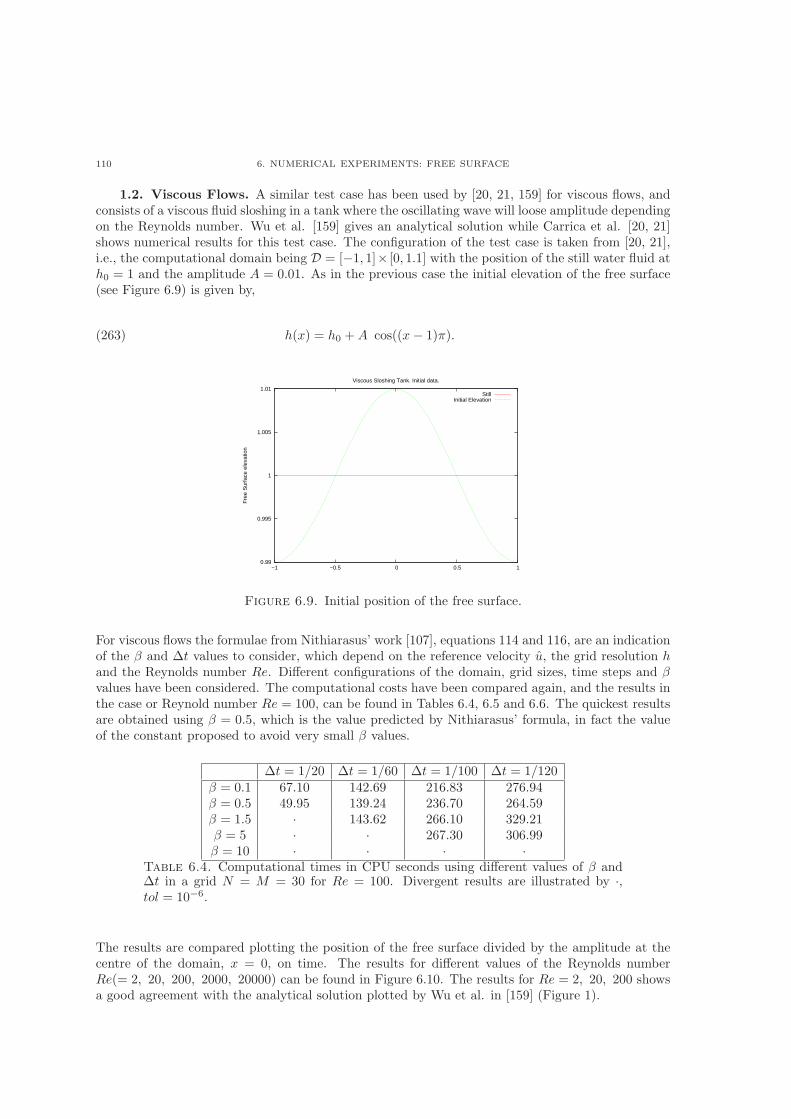
110 6. NUMERICAL EXPERIMENTS: FREE SURFACE
1.2. Viscous Flows. A similar test case has been used by [20, 21, 159] for viscous flows, andconsists of a viscous fluid sloshing in a tank where the oscillating wave will loose amplitude dependingon the Reynolds number. Wu et al. [159] gives an analytical solution while Carrica et al. [20, 21]shows numerical results for this test case. The configuration of the test case is taken from [20, 21],i.e., the computational domain being D = [−1, 1]× [0, 1.1] with the position of the still water fluid atℎ0 = 1 and the amplitude A = 0.01. As in the previous case the initial elevation of the free surface(see Figure 6.9) is given by,
ℎ(x) = ℎ0 +A cos((x− 1)�).(263)
0.99
0.995
1
1.005
1.01
−1 −0.5 0 0.5 1
Fre
e S
urfa
ce e
leva
tion
Viscous Sloshing Tank. Initial data.
StillInitial Elevation
Figure 6.9. Initial position of the free surface.
For viscous flows the formulae from Nithiarasus’ work [107], equations 114 and 116, are an indicationof the � and Δt values to consider, which depend on the reference velocity u, the grid resolution ℎand the Reynolds number Re. Different configurations of the domain, grid sizes, time steps and �values have been considered. The computational costs have been compared again, and the results inthe case or Reynold number Re = 100, can be found in Tables 6.4, 6.5 and 6.6. The quickest resultsare obtained using � = 0.5, which is the value predicted by Nithiarasus’ formula, in fact the valueof the constant proposed to avoid very small � values.
Δt = 1/20 Δt = 1/60 Δt = 1/100 Δt = 1/120� = 0.1 67.10 142.69 216.83 276.94� = 0.5 49.95 139.24 236.70 264.59� = 1.5 ⋅ 143.62 266.10 329.21� = 5 ⋅ ⋅ 267.30 306.99� = 10 ⋅ ⋅ ⋅ ⋅
Table 6.4. Computational times in CPU seconds using different values of � andΔt in a grid N = M = 30 for Re = 100. Divergent results are illustrated by ⋅,tol = 10−6.
The results are compared plotting the position of the free surface divided by the amplitude at thecentre of the domain, x = 0, on time. The results for different values of the Reynolds numberRe(= 2, 20, 200, 2000, 20000) can be found in Figure 6.10. The results for Re = 2, 20, 200 showsa good agreement with the analytical solution plotted by Wu et al. in [159] (Figure 1).
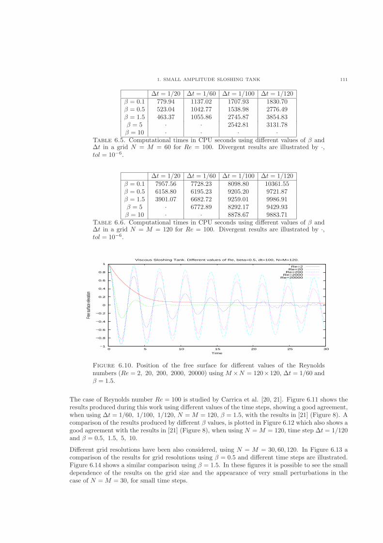
1. SMALL AMPLITUDE SLOSHING TANK 111
Δt = 1/20 Δt = 1/60 Δt = 1/100 Δt = 1/120� = 0.1 779.94 1137.02 1707.93 1830.70� = 0.5 523.04 1042.77 1538.98 2776.49� = 1.5 463.37 1055.86 2745.87 3854.83� = 5 ⋅ ⋅ 2542.81 3131.78� = 10 ⋅ ⋅ ⋅ ⋅
Table 6.5. Computational times in CPU seconds using different values of � andΔt in a grid N = M = 60 for Re = 100. Divergent results are illustrated by ⋅,tol = 10−6.
Δt = 1/20 Δt = 1/60 Δt = 1/100 Δt = 1/120� = 0.1 7957.56 7728.23 8098.80 10361.55� = 0.5 6158.80 6195.23 9205.20 9721.87� = 1.5 3901.07 6682.72 9259.01 9986.91� = 5 ⋅ 6772.89 8292.17 9429.93� = 10 ⋅ ⋅ 8878.67 9883.71
Table 6.6. Computational times in CPU seconds using different values of � andΔt in a grid N = M = 120 for Re = 100. Divergent results are illustrated by ⋅,tol = 10−6.
−1
−0.8
−0.6
−0.4
−0.2
0
0.2
0.4
0.6
0.8
1
0 5 10 15 20 25 30
Free s
urfac
e elev
ation
Time
Viscous Sloshing Tank. Different values of Re, beta=0.5, dt=100, N=M=120.
Re=2Re=20
Re=200Re=2000
Re=20000
Figure 6.10. Position of the free surface for different values of the Reynoldsnumbers (Re = 2, 20, 200, 2000, 20000) using M ×N = 120×120, Δt = 1/60 and� = 1.5.
The case of Reynolds number Re = 100 is studied by Carrica et al. [20, 21]. Figure 6.11 shows theresults produced during this work using different values of the time steps, showing a good agreement,when using Δt = 1/60, 1/100, 1/120, N =M = 120, � = 1.5, with the results in [21] (Figure 8). Acomparison of the results produced by different � values, is plotted in Figure 6.12 which also shows agood agreement with the results in [21] (Figure 8), when using N =M = 120, time step Δt = 1/120and � = 0.5, 1.5, 5, 10.
Different grid resolutions have been also considered, using N = M = 30, 60, 120. In Figure 6.13 acomparison of the results for grid resolutions using � = 0.5 and different time steps are illustrated.Figure 6.14 shows a similar comparison using � = 1.5. In these figures it is possible to see the smalldependence of the results on the grid size and the appearance of very small perturbations in thecase of N =M = 30, for small time steps.
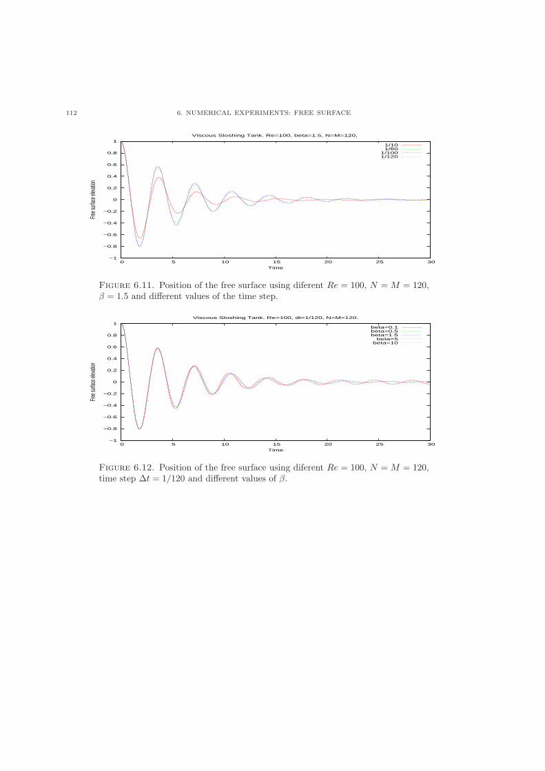
112 6. NUMERICAL EXPERIMENTS: FREE SURFACE
−1
−0.8
−0.6
−0.4
−0.2
0
0.2
0.4
0.6
0.8
1
0 5 10 15 20 25 30
Free s
urfac
e elev
ation
Time
Viscous Sloshing Tank. Re=100, beta=1.5, N=M=120,
1/101/60
1/1001/120
Figure 6.11. Position of the free surface using diferent Re = 100, N = M = 120,� = 1.5 and different values of the time step.
−1
−0.8
−0.6
−0.4
−0.2
0
0.2
0.4
0.6
0.8
1
0 5 10 15 20 25 30
Free s
urfac
e elev
ation
Time
Viscous Sloshing Tank. Re=100, dt=1/120, N=M=120.
beta=0.1beta=0.5beta=1.5
beta=5beta=10
Figure 6.12. Position of the free surface using diferent Re = 100, N = M = 120,time step Δt = 1/120 and different values of �.
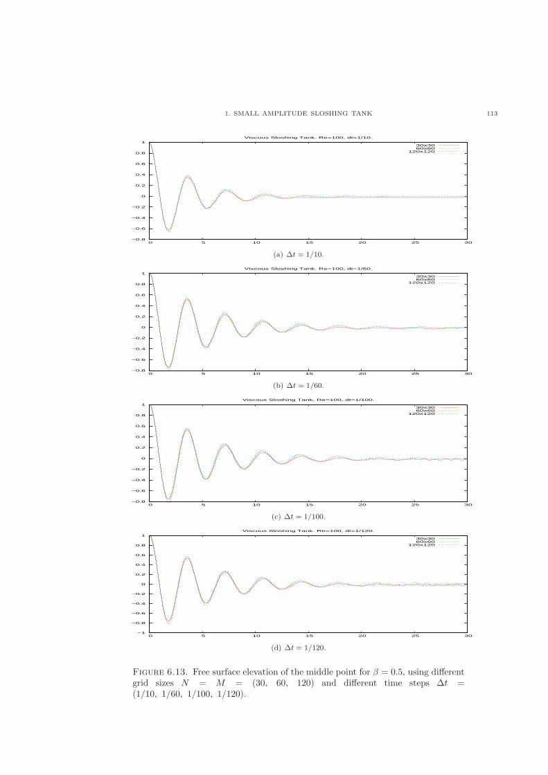
1. SMALL AMPLITUDE SLOSHING TANK 113
−0.8
−0.6
−0.4
−0.2
0
0.2
0.4
0.6
0.8
1
0 5 10 15 20 25 30
Viscous Sloshing Tank. Re=100, dt=1/10.
30x3060x60
120x120
(a) Δt = 1/10.
−0.8
−0.6
−0.4
−0.2
0
0.2
0.4
0.6
0.8
1
0 5 10 15 20 25 30
Viscous Sloshing Tank. Re=100, dt=1/60.
30x3060x60
120x120
(b) Δt = 1/60.
−0.8
−0.6
−0.4
−0.2
0
0.2
0.4
0.6
0.8
1
0 5 10 15 20 25 30
Viscous Sloshing Tank. Re=100, dt=1/100.
30x3060x60
120x120
(c) Δt = 1/100.
−1
−0.8
−0.6
−0.4
−0.2
0
0.2
0.4
0.6
0.8
1
0 5 10 15 20 25 30
Viscous Sloshing Tank. Re=100, dt=1/120.
30x3060x60
120x120
(d) Δt = 1/120.
Figure 6.13. Free surface elevation of the middle point for � = 0.5, using differentgrid sizes N = M = (30, 60, 120) and different time steps Δt =(1/10, 1/60, 1/100, 1/120).
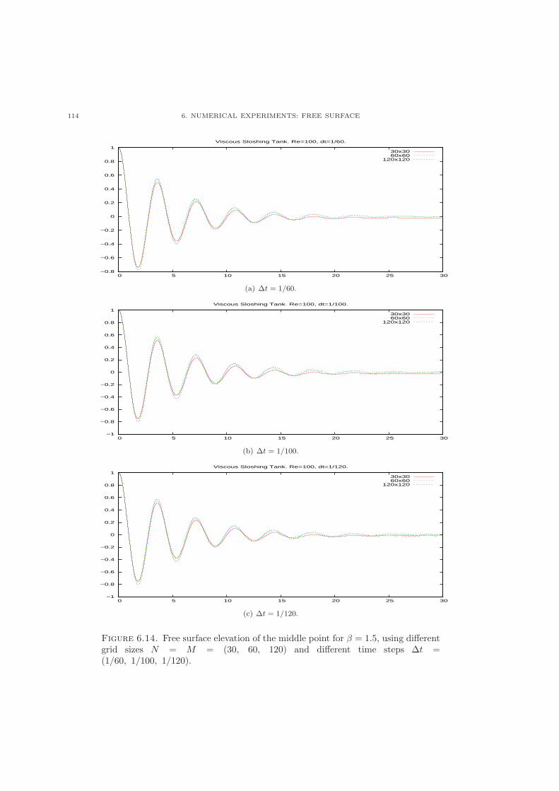
114 6. NUMERICAL EXPERIMENTS: FREE SURFACE
−0.8
−0.6
−0.4
−0.2
0
0.2
0.4
0.6
0.8
1
0 5 10 15 20 25 30
Viscous Sloshing Tank. Re=100, dt=1/60.
30x3060x60
120x120
(a) Δt = 1/60.
−1
−0.8
−0.6
−0.4
−0.2
0
0.2
0.4
0.6
0.8
1
0 5 10 15 20 25 30
Viscous Sloshing Tank. Re=100, dt=1/100.
30x3060x60
120x120
(b) Δt = 1/100.
−1
−0.8
−0.6
−0.4
−0.2
0
0.2
0.4
0.6
0.8
1
0 5 10 15 20 25 30
Viscous Sloshing Tank. Re=100, dt=1/120.
30x3060x60
120x120
(c) Δt = 1/120.
Figure 6.14. Free surface elevation of the middle point for � = 1.5, using differentgrid sizes N = M = (30, 60, 120) and different time steps Δt =(1/60, 1/100, 1/120).
2. MASS-WAVE MAKER 115
2. Mass-Wave Maker
An interesting numerical experiment for the case of inviscid flow is the mass-wave maker describedby Lin and Liu in [82]. Fluid at rest is perturbed by a mass source producing regular waves whichamplitude remains constant without loss of amplitude. The computational domain considered isΩ = [0, 9.98]× [0, 0.2125], where the undisturbed free surface is placed at y = 0.2 and the source ofmass is placed in the flow, see Figure 6.15.
��������
��������
Figure 6.15. Scheme of the mass-wave maker problem. The red square representsthe area of the mass source.
The source function for regular waves described in [82] is,
s(t) =CH
Asin(�t),(264)
where C is a constant (in this work the value is C = 1.21 m/s), H the amplitude, � = 2� the wavefrequency, A the area of the source which makes the wave period T to be T = 1.
The numerical experiment tested used open boundaries with value of H = 0.01 m, and the masssource placed at y = d/3 below the free surface label an d = 0.2 with area A = 15ΔxΔy. The com-putational grid is uniform over Ω with N = 201 and M = 50 and time step of Δt = 1/500 seconds.The results obtained in Figure 6.16 show similar behaviour to those obtained in the case of theinviscid sloshing tank where there is a damping in the amplitude of the waves, which is incrementedas the artificial compressibility parameter � grows.
The computational times required for different � values are different, for example, using � = 500the program takes 8099.69 CPU seconds, using � = 2000 takes 9606.67 CPU seconds and with� = 200000 takes 16776.57 CPU seconds. The computational times, and the number of pseudo-timesteps needed between consecutive time steps grows with �.
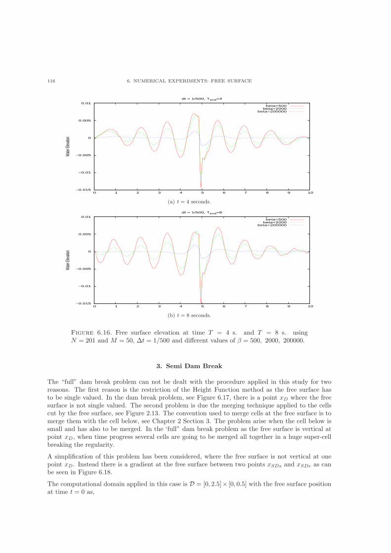
116 6. NUMERICAL EXPERIMENTS: FREE SURFACE
−0.015
−0.01
−0.005
0
0.005
0.01
0 1 2 3 4 5 6 7 8 9 10
Water
Elev
ation
dt = 1/500, Tend=4
beta=500beta=2000
beta=200000
(a) t = 4 seconds.
−0.015
−0.01
−0.005
0
0.005
0.01
0 1 2 3 4 5 6 7 8 9 10
Water
Elev
ation
dt = 1/500, Tend=8
beta=500beta=2000
beta=200000
(b) t = 8 seconds.
Figure 6.16. Free surface elevation at time T = 4 s. and T = 8 s. usingN = 201 and M = 50, Δt = 1/500 and different values of � = 500, 2000, 200000.
3. Semi Dam Break
The “full” dam break problem can not be dealt with the procedure applied in this study for tworeasons. The first reason is the restriction of the Height Function method as the free surface hasto be single valued. In the dam break problem, see Figure 6.17, there is a point xD where the freesurface is not single valued. The second problem is due the merging technique applied to the cellscut by the free surface, see Figure 2.13. The convention used to merge cells at the free surface is tomerge them with the cell below, see Chapter 2 Section 3. The problem arise when the cell below issmall and has also to be merged. In the ‘full” dam break problem as the free surface is vertical atpoint xD, when time progress several cells are going to be merged all together in a huge super-cellbreaking the regularity.
A simplification of this problem has been considered, where the free surface is not vertical at onepoint xD. Instead there is a gradient at the free surface between two points xSDs and xSDe as canbe seen in Figure 6.18.
The computational domain applied in this case is D = [0, 2.5]× [0, 0.5] with the free surface positionat time t = 0 as,
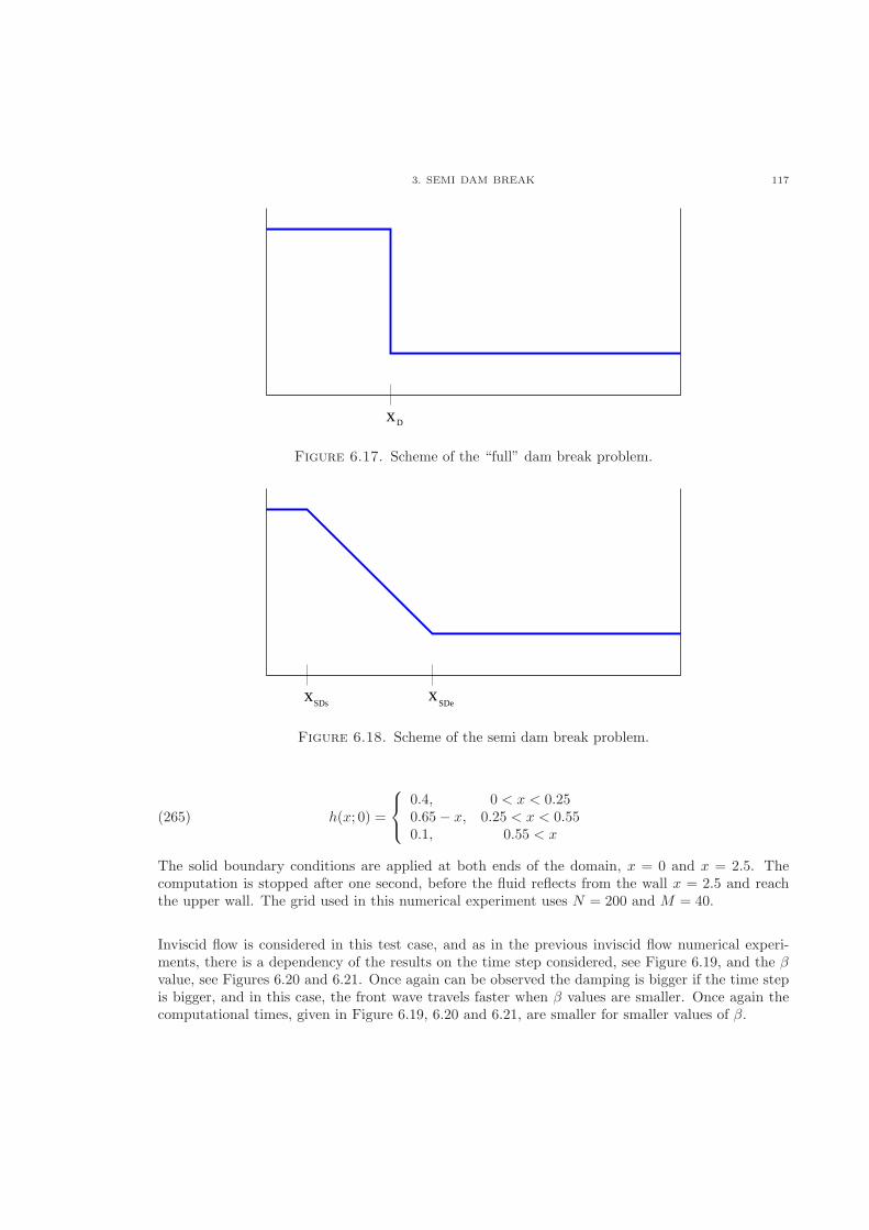
3. SEMI DAM BREAK 117
xD
Figure 6.17. Scheme of the “full” dam break problem.
x xSDs SDe
Figure 6.18. Scheme of the semi dam break problem.
ℎ(x; 0) =
⎧
⎨
⎩
0.4, 0 < x < 0.250.65− x, 0.25 < x < 0.550.1, 0.55 < x
(265)
The solid boundary conditions are applied at both ends of the domain, x = 0 and x = 2.5. Thecomputation is stopped after one second, before the fluid reflects from the wall x = 2.5 and reachthe upper wall. The grid used in this numerical experiment uses N = 200 and M = 40.
Inviscid flow is considered in this test case, and as in the previous inviscid flow numerical experi-ments, there is a dependency of the results on the time step considered, see Figure 6.19, and the �value, see Figures 6.20 and 6.21. Once again can be observed the damping is bigger if the time stepis bigger, and in this case, the front wave travels faster when � values are smaller. Once again thecomputational times, given in Figure 6.19, 6.20 and 6.21, are smaller for smaller values of �.
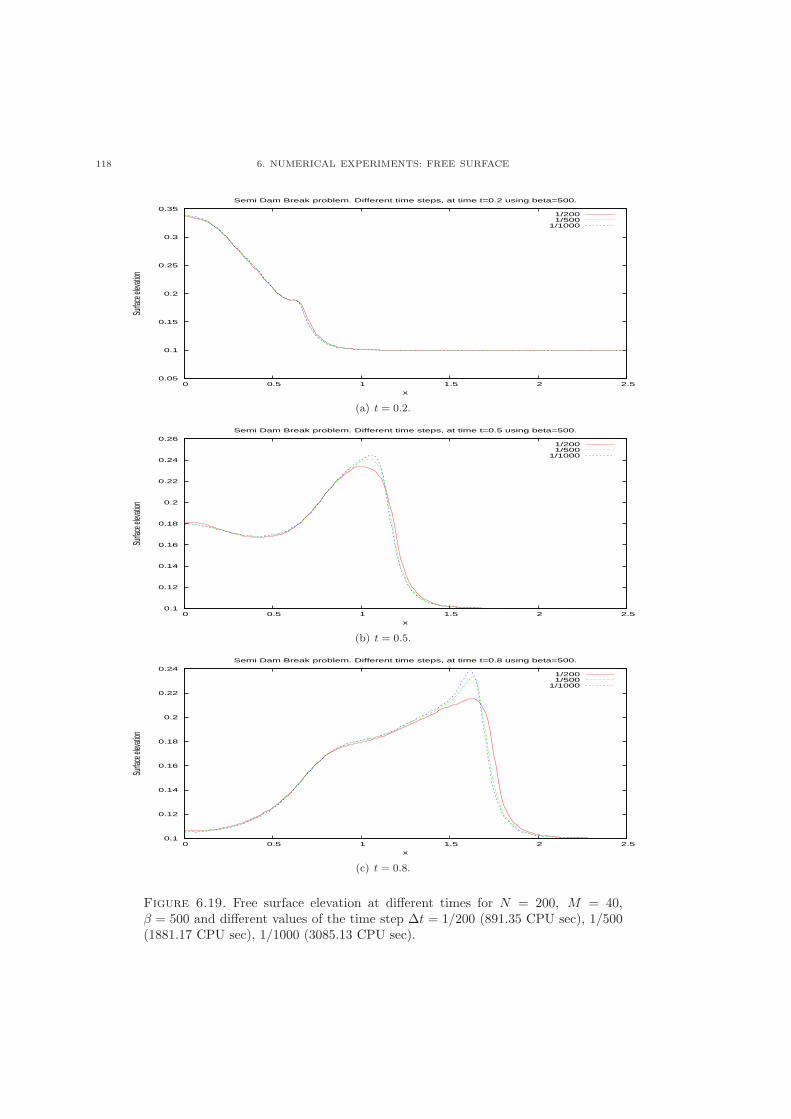
118 6. NUMERICAL EXPERIMENTS: FREE SURFACE
0.05
0.1
0.15
0.2
0.25
0.3
0.35
0 0.5 1 1.5 2 2.5
Surfa
ce el
evati
on
x
Semi Dam Break problem. Different time steps, at time t=0.2 using beta=500.
1/2001/500
1/1000
(a) t = 0.2.
0.1
0.12
0.14
0.16
0.18
0.2
0.22
0.24
0.26
0 0.5 1 1.5 2 2.5
Surfa
ce el
evati
on
x
Semi Dam Break problem. Different time steps, at time t=0.5 using beta=500.
1/2001/500
1/1000
(b) t = 0.5.
0.1
0.12
0.14
0.16
0.18
0.2
0.22
0.24
0 0.5 1 1.5 2 2.5
Surfa
ce el
evati
on
x
Semi Dam Break problem. Different time steps, at time t=0.8 using beta=500.
1/2001/500
1/1000
(c) t = 0.8.
Figure 6.19. Free surface elevation at different times for N = 200, M = 40,� = 500 and different values of the time step Δt = 1/200 (891.35 CPU sec), 1/500(1881.17 CPU sec), 1/1000 (3085.13 CPU sec).
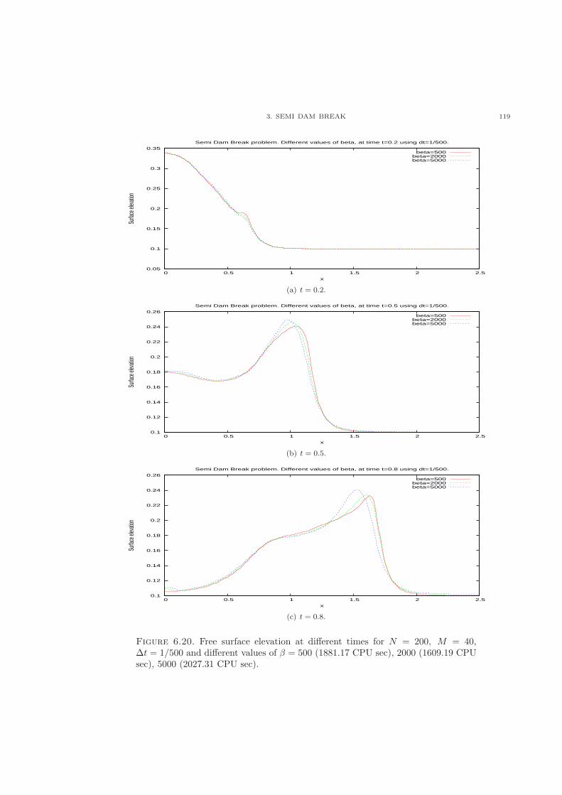
3. SEMI DAM BREAK 119
0.05
0.1
0.15
0.2
0.25
0.3
0.35
0 0.5 1 1.5 2 2.5
Surfa
ce el
evati
on
x
Semi Dam Break problem. Different values of beta, at time t=0.2 using dt=1/500.
beta=500beta=2000beta=5000
(a) t = 0.2.
0.1
0.12
0.14
0.16
0.18
0.2
0.22
0.24
0.26
0 0.5 1 1.5 2 2.5
Surfa
ce el
evati
on
x
Semi Dam Break problem. Different values of beta, at time t=0.5 using dt=1/500.
beta=500beta=2000beta=5000
(b) t = 0.5.
0.1
0.12
0.14
0.16
0.18
0.2
0.22
0.24
0.26
0 0.5 1 1.5 2 2.5
Surfa
ce el
evati
on
x
Semi Dam Break problem. Different values of beta, at time t=0.8 using dt=1/500.
beta=500beta=2000beta=5000
(c) t = 0.8.
Figure 6.20. Free surface elevation at different times for N = 200, M = 40,Δt = 1/500 and different values of � = 500 (1881.17 CPU sec), 2000 (1609.19 CPUsec), 5000 (2027.31 CPU sec).
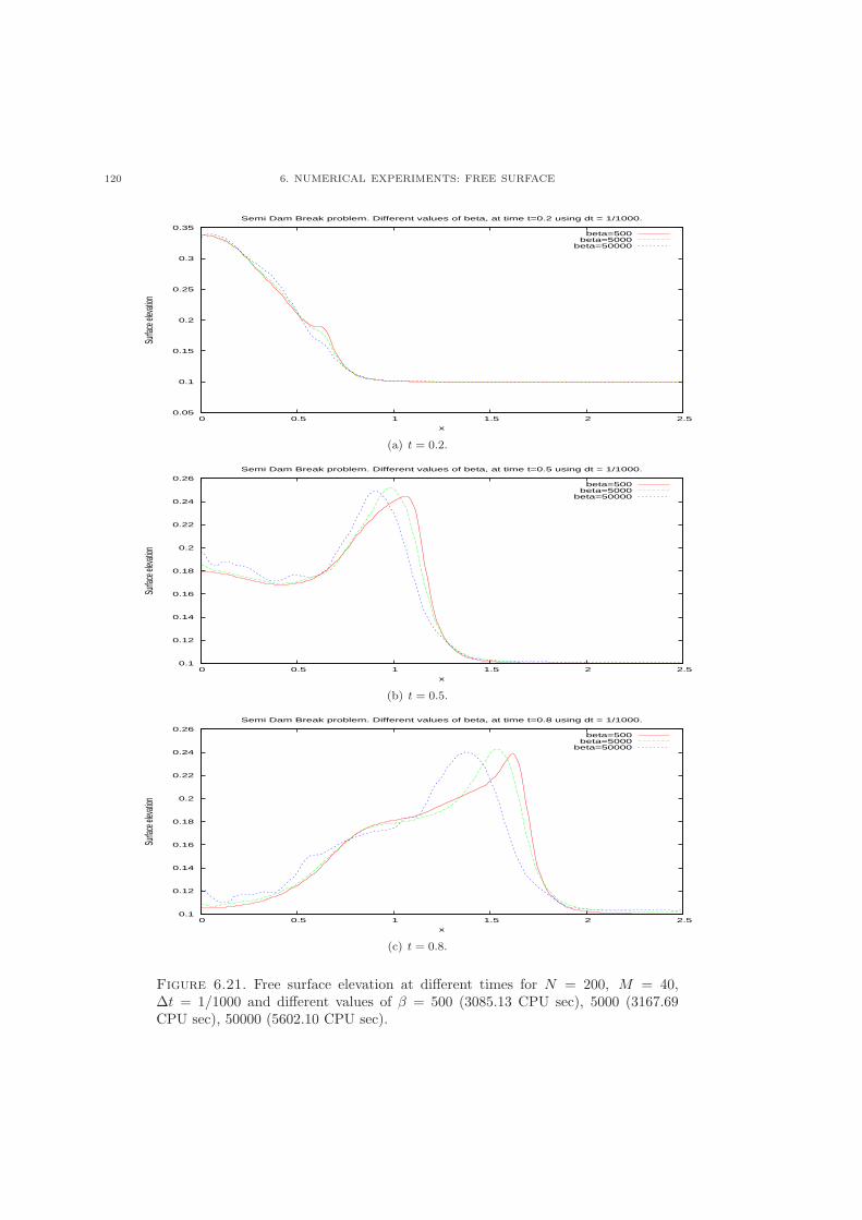
120 6. NUMERICAL EXPERIMENTS: FREE SURFACE
0.05
0.1
0.15
0.2
0.25
0.3
0.35
0 0.5 1 1.5 2 2.5
Surfa
ce el
evati
on
x
Semi Dam Break problem. Different values of beta, at time t=0.2 using dt = 1/1000.
beta=500beta=5000
beta=50000
(a) t = 0.2.
0.1
0.12
0.14
0.16
0.18
0.2
0.22
0.24
0.26
0 0.5 1 1.5 2 2.5
Surfa
ce el
evati
on
x
Semi Dam Break problem. Different values of beta, at time t=0.5 using dt = 1/1000.
beta=500beta=5000
beta=50000
(b) t = 0.5.
0.1
0.12
0.14
0.16
0.18
0.2
0.22
0.24
0.26
0 0.5 1 1.5 2 2.5
Surfa
ce el
evati
on
x
Semi Dam Break problem. Different values of beta, at time t=0.8 using dt = 1/1000.
beta=500beta=5000
beta=50000
(c) t = 0.8.
Figure 6.21. Free surface elevation at different times for N = 200, M = 40,Δt = 1/1000 and different values of � = 500 (3085.13 CPU sec), 5000 (3167.69CPU sec), 50000 (5602.10 CPU sec).
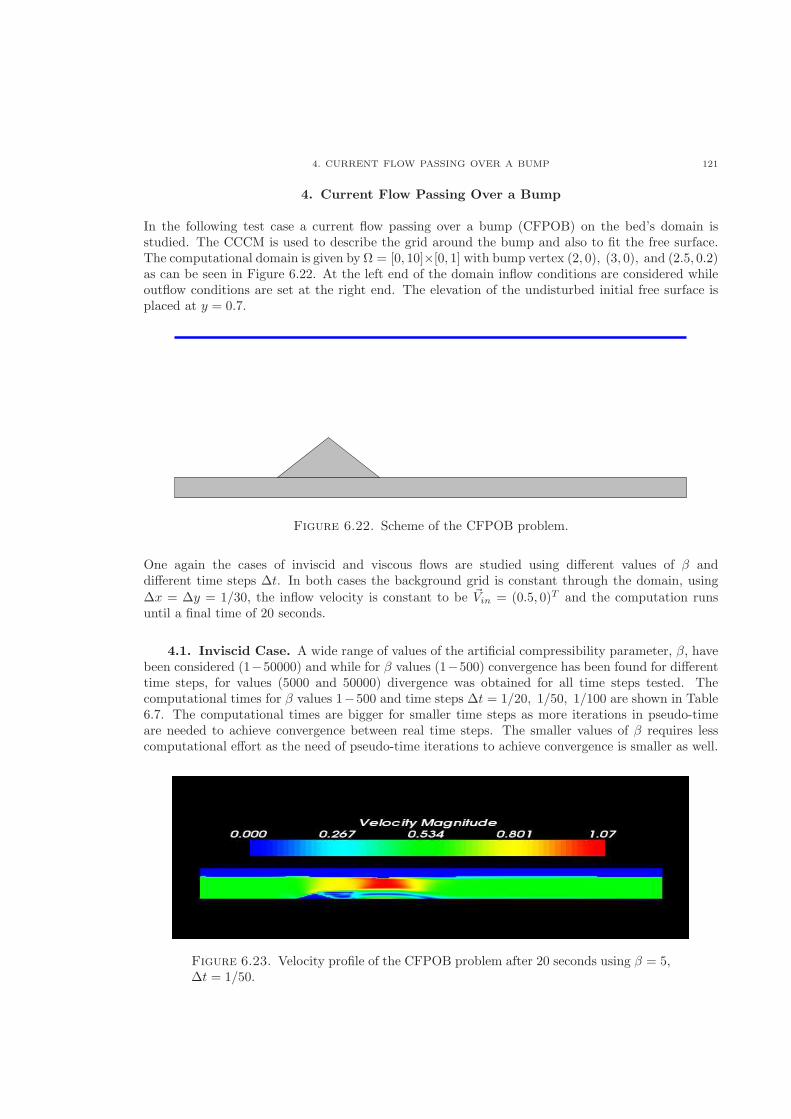
4. CURRENT FLOW PASSING OVER A BUMP 121
4. Current Flow Passing Over a Bump
In the following test case a current flow passing over a bump (CFPOB) on the bed’s domain isstudied. The CCCM is used to describe the grid around the bump and also to fit the free surface.The computational domain is given by Ω = [0, 10]×[0, 1] with bump vertex (2, 0), (3, 0), and (2.5, 0.2)as can be seen in Figure 6.22. At the left end of the domain inflow conditions are considered whileoutflow conditions are set at the right end. The elevation of the undisturbed initial free surface isplaced at y = 0.7.
Figure 6.22. Scheme of the CFPOB problem.
One again the cases of inviscid and viscous flows are studied using different values of � anddifferent time steps Δt. In both cases the background grid is constant through the domain, using
Δx = Δy = 1/30, the inflow velocity is constant to be Vin = (0.5, 0)T and the computation runsuntil a final time of 20 seconds.
4.1. Inviscid Case. A wide range of values of the artificial compressibility parameter, �, havebeen considered (1−50000) and while for � values (1−500) convergence has been found for differenttime steps, for values (5000 and 50000) divergence was obtained for all time steps tested. Thecomputational times for � values 1−500 and time steps Δt = 1/20, 1/50, 1/100 are shown in Table6.7. The computational times are bigger for smaller time steps as more iterations in pseudo-timeare needed to achieve convergence between real time steps. The smaller values of � requires lesscomputational effort as the need of pseudo-time iterations to achieve convergence is smaller as well.
Figure 6.23. Velocity profile of the CFPOB problem after 20 seconds using � = 5,Δt = 1/50.
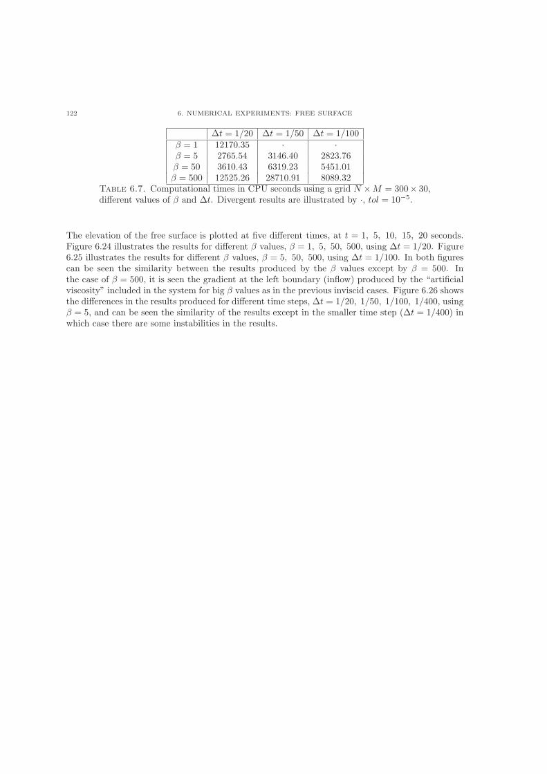
122 6. NUMERICAL EXPERIMENTS: FREE SURFACE
Δt = 1/20 Δt = 1/50 Δt = 1/100� = 1 12170.35 ⋅ ⋅� = 5 2765.54 3146.40 2823.76� = 50 3610.43 6319.23 5451.01� = 500 12525.26 28710.91 8089.32
Table 6.7. Computational times in CPU seconds using a grid N ×M = 300× 30,different values of � and Δt. Divergent results are illustrated by ⋅, tol = 10−5.
The elevation of the free surface is plotted at five different times, at t = 1, 5, 10, 15, 20 seconds.Figure 6.24 illustrates the results for different � values, � = 1, 5, 50, 500, using Δt = 1/20. Figure6.25 illustrates the results for different � values, � = 5, 50, 500, using Δt = 1/100. In both figurescan be seen the similarity between the results produced by the � values except by � = 500. Inthe case of � = 500, it is seen the gradient at the left boundary (inflow) produced by the “artificialviscosity” included in the system for big � values as in the previous inviscid cases. Figure 6.26 showsthe differences in the results produced for different time steps, Δt = 1/20, 1/50, 1/100, 1/400, using� = 5, and can be seen the similarity of the results except in the smaller time step (Δt = 1/400) inwhich case there are some instabilities in the results.
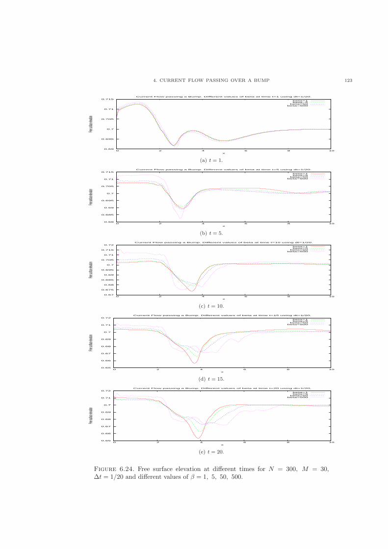
4. CURRENT FLOW PASSING OVER A BUMP 123
0.69
0.695
0.7
0.705
0.71
0.715
0 2 4 6 8 10
Free surf
ace elev
ation
x
Current Flow passing a Bump. Different values of beta at time t=1 using dt=1/20.
beta=1beta=5
beta=50beta=500
(a) t = 1.
0.68
0.685
0.69
0.695
0.7
0.705
0.71
0.715
0 2 4 6 8 10
Free surf
ace elev
ation
x
Current Flow passing a Bump. Different values of beta at time t=5 using dt=1/20.
beta=1beta=5
beta=50beta=500
(b) t = 5.
0.67
0.675
0.68
0.685
0.69
0.695
0.7
0.705
0.71
0.715
0.72
0 2 4 6 8 10
Free surf
ace elev
ation
x
Current Flow passing a Bump. Different values of beta at time t=10 using dt=1/20.
beta=1beta=5
beta=50beta=500
(c) t = 10.
0.65
0.66
0.67
0.68
0.69
0.7
0.71
0.72
0 2 4 6 8 10
Free surf
ace elev
ation
x
Current Flow passing a Bump. Different values of beta at time t=15 using dt=1/20.
beta=1beta=5
beta=50beta=500
(d) t = 15.
0.65
0.66
0.67
0.68
0.69
0.7
0.71
0.72
0 2 4 6 8 10
Free surf
ace elev
ation
x
Current Flow passing a Bump. Different values of beta at time t=20 using dt=1/20.
beta=1beta=5
beta=50beta=500
(e) t = 20.
Figure 6.24. Free surface elevation at different times for N = 300, M = 30,Δt = 1/20 and different values of � = 1, 5, 50, 500.
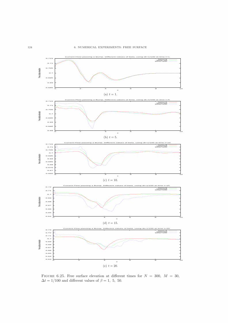
124 6. NUMERICAL EXPERIMENTS: FREE SURFACE
0.685
0.69
0.695
0.7
0.705
0.71
0.715
0 2 4 6 8 10
Free surf
ace elev
ation
x
Current Flow passing a Bump. Different values of beta, using dt=1/100 at time t=1.
beta=5beta=50
beta=500
(a) t = 1.
0.68
0.685
0.69
0.695
0.7
0.705
0.71
0.715
0 2 4 6 8 10
Free surf
ace elev
ation
x
Current Flow passing a Bump. Different values of beta, using dt=1/100 at time t=5.
beta=5beta=50
beta=500
(b) t = 5.
0.665
0.67
0.675
0.68
0.685
0.69
0.695
0.7
0.705
0.71
0.715
0 2 4 6 8 10
Free surf
ace elev
ation
x
Current Flow passing a Bump. Different values of beta, using dt=1/100 at time t=10.
beta=5beta=50
beta=500
(c) t = 10.
0.64
0.65
0.66
0.67
0.68
0.69
0.7
0.71
0.72
0 2 4 6 8 10
Free surf
ace elev
ation
x
Current Flow passing a Bump. Different values of beta, using dt=1/100 at time t=15.
beta=5beta=50
beta=500
(d) t = 15.
0.63
0.64
0.65
0.66
0.67
0.68
0.69
0.7
0.71
0.72
0.73
0 2 4 6 8 10
Free surf
ace elev
ation
x
Current Flow passing a Bump. Different values of beta, using dt=1/100 at time t=20.
beta=5beta=50
beta=500
(e) t = 20.
Figure 6.25. Free surface elevation at different times for N = 300, M = 30,Δt = 1/100 and different values of � = 1, 5, 50.
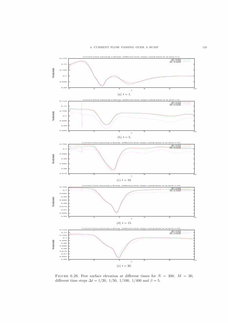
4. CURRENT FLOW PASSING OVER A BUMP 125
0.69
0.695
0.7
0.705
0.71
0.715
0 2 4 6 8 10
Free surf
ace elev
ation
x
Current Flow passing a Bump. Different time steps using beta=5 at time t=1.
dt=1/20dt=1/50
dt=1/100dt=1/400
(a) t = 1.
0.685
0.69
0.695
0.7
0.705
0.71
0.715
0 2 4 6 8 10
Free surf
ace elev
ation
x
Current Flow passing a Bump. Different time steps using beta=5 at time t=5.
dt=1/20dt=1/50
dt=1/100dt=1/400
(b) t = 5.
0.675
0.68
0.685
0.69
0.695
0.7
0.705
0 2 4 6 8 10
Free surf
ace elev
ation
x
Current Flow passing a Bump. Different time steps using beta=5 at time t=10.
dt=1/20dt=1/50
dt=1/100dt=1/400
(c) t = 10.
0.66
0.665
0.67
0.675
0.68
0.685
0.69
0.695
0.7
0.705
0 2 4 6 8 10
Free surf
ace elev
ation
x
Current Flow passing a Bump. Different time steps using beta=5 at time t=15.
dt=1/20dt=1/50
dt=1/100dt=1/400
(d) t = 15.
0.66
0.665
0.67
0.675
0.68
0.685
0.69
0.695
0.7
0.705
0.71
0.715
0 2 4 6 8 10
Free surf
ace elev
ation
x
Current Flow passing a Bump. Different time steps using beta=5 at time t=20.
dt=1/20dt=1/50
dt=1/100dt=1/400
(e) t = 20.
Figure 6.26. Free surface elevation at different times for N = 300, M = 30,different time steps Δt = 1/20, 1/50, 1/100, 1/400 and � = 5.
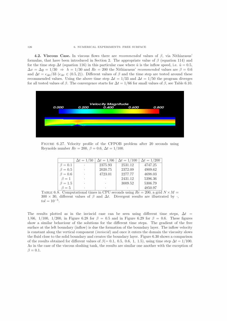
126 6. NUMERICAL EXPERIMENTS: FREE SURFACE
4.2. Viscous Case. In viscous flows there are recommended values of �, via Nithiarasus’formulas, that have been introduced in Section 2. The appropriate value of � (equation 114) andfor the time step Δt (equation 116) in this particular case where u is the inflow speed, i.e. u = 0.5,Δx = Δy = 1/30 ⇒ ℎ = 1/30 and Re = 200 the Nithiarasus’ recommended values are � = 0.6and Δt = �Δt/33 (�Δt ∈ (0.5, 2)). Different values of � and the time step are tested around theserecommended values. Using the above time step Δt = 1/33 and Δt = 1/50 the program divergesfor all tested values of �. The convergence starts for Δt = 1/66 for small values of �, see Table 6.10.
Figure 6.27. Velocity profile of the CFPOB problem after 20 seconds usingReynolds number Re = 200, � = 0.6, Δt = 1/100.
Δt = 1/50 Δt = 1/66 Δt = 1/100 Δt = 1/200� = 0.1 ⋅ 2375.93 2531.12 4747.25� = 0.5 ⋅ 2020.75 2372.09 4909.62� = 0.6 ⋅ 4723.01 2277.77 4698.03� = 1 ⋅ ⋅ 2431.12 5396.36� = 1.5 ⋅ ⋅ 3009.52 5306.79� = 5 ⋅ ⋅ ⋅ 4850.97
Table 6.8. Computational times in CPU seconds using Re = 200, a grid N×M =300 × 30, different values of � and Δt. Divergent results are illustrated by ⋅,tol = 10−5.
The results plotted as in the inviscid case can be seen using different time steps, Δt =1/66, 1/100, 1/200, in Figure 6.28 for � = 0.5 and in Figure 6.29 for � = 0.6. These figuresshow a similar behaviour of the solutions for the different time steps. The gradient of the freesurface at the left boundary (inflow) is due the formation of the boundary layer. The inflow velocityis constant along the vertical component (inviscid) and once it enters the domain the viscosity slowsthe fluid close to the solid boundary and creates the boundary layer. Figure 6.30 shows a comparisonof the results obtained for different values of �(= 0.1, 0.5, 0.6, 1, 1.5), using time step Δt = 1/100.As in the case of the viscous sloshing tank, the results are similar one another with the exception of� = 0.1.
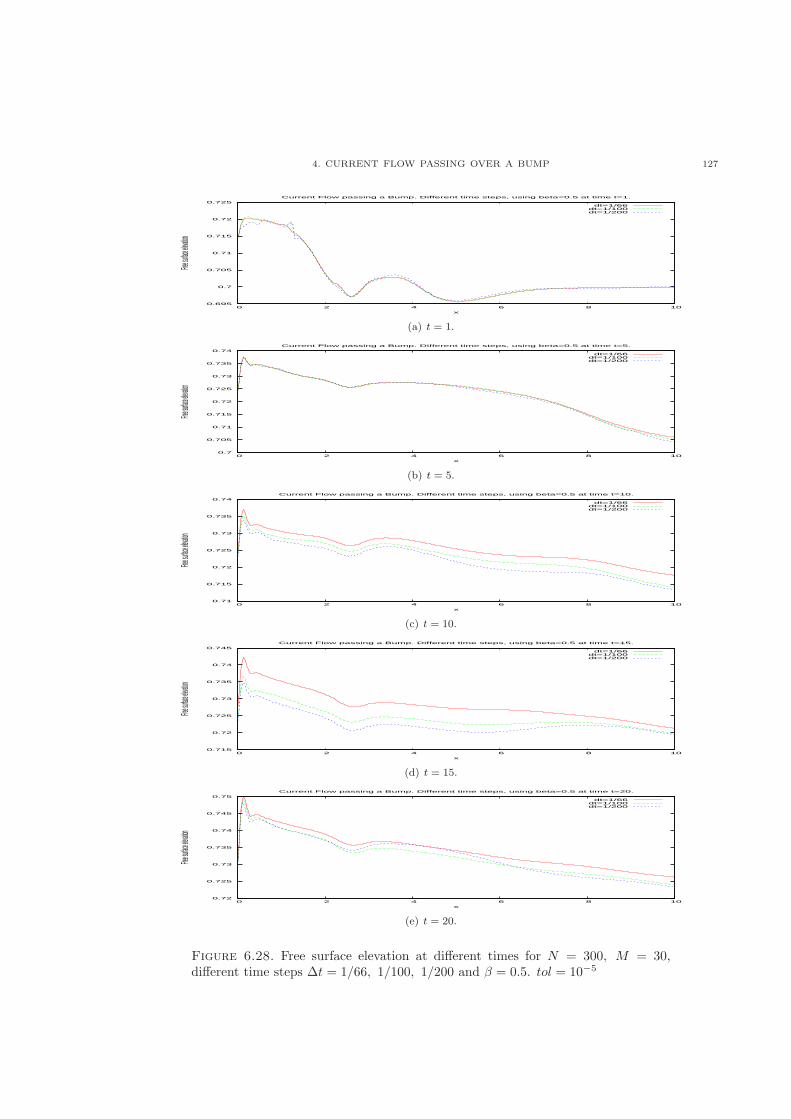
4. CURRENT FLOW PASSING OVER A BUMP 127
0.695
0.7
0.705
0.71
0.715
0.72
0.725
0 2 4 6 8 10
Free surf
ace elev
ation
x
Current Flow passing a Bump. Different time steps, using beta=0.5 at time t=1.
dt=1/66dt=1/100dt=1/200
(a) t = 1.
0.7
0.705
0.71
0.715
0.72
0.725
0.73
0.735
0.74
0 2 4 6 8 10
Free surf
ace elev
ation
x
Current Flow passing a Bump. Different time steps, using beta=0.5 at time t=5.
dt=1/66dt=1/100dt=1/200
(b) t = 5.
0.71
0.715
0.72
0.725
0.73
0.735
0.74
0 2 4 6 8 10
Free surf
ace elev
ation
x
Current Flow passing a Bump. Different time steps, using beta=0.5 at time t=10.
dt=1/66dt=1/100dt=1/200
(c) t = 10.
0.715
0.72
0.725
0.73
0.735
0.74
0.745
0 2 4 6 8 10
Free surf
ace elev
ation
x
Current Flow passing a Bump. Different time steps, using beta=0.5 at time t=15.
dt=1/66dt=1/100dt=1/200
(d) t = 15.
0.72
0.725
0.73
0.735
0.74
0.745
0.75
0 2 4 6 8 10
Free surf
ace elev
ation
x
Current Flow passing a Bump. Different time steps, using beta=0.5 at time t=20.
dt=1/66dt=1/100dt=1/200
(e) t = 20.
Figure 6.28. Free surface elevation at different times for N = 300, M = 30,different time steps Δt = 1/66, 1/100, 1/200 and � = 0.5. tol = 10−5
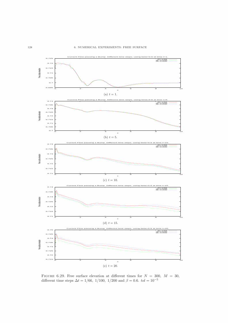
128 6. NUMERICAL EXPERIMENTS: FREE SURFACE
0.695
0.7
0.705
0.71
0.715
0.72
0.725
0 2 4 6 8 10
Free surf
ace elev
ation
x
Current Flow passing a Bump. Different time steps, using beta=0.6 at time t=1.
dt=1/66dt=1/100dt=1/200
(a) t = 1.
0.7
0.705
0.71
0.715
0.72
0.725
0.73
0.735
0.74
0 2 4 6 8 10
Free surf
ace elev
ation
x
Current Flow passing a Bump. Different time steps, using beta=0.6 at time t=5.
dt=1/66dt=1/100dt=1/200
(b) t = 5.
0.71
0.715
0.72
0.725
0.73
0.735
0.74
0 2 4 6 8 10
Free surf
ace elev
ation
x
Current Flow passing a Bump. Different time steps, using beta=0.6 at time t=10.
dt=1/66dt=1/100dt=1/200
(c) t = 10.
0.71
0.715
0.72
0.725
0.73
0.735
0.74
0 2 4 6 8 10
Free surf
ace elev
ation
x
Current Flow passing a Bump. Different time steps, using beta=0.6 at time t=15.
dt=1/66dt=1/100dt=1/200
(d) t = 15.
0.715
0.72
0.725
0.73
0.735
0.74
0.745
0.75
0 2 4 6 8 10
Free surf
ace elev
ation
x
Current Flow passing a Bump. Different time steps, using beta=0.6 at time t=20.
dt=1/66dt=1/100dt=1/200
(e) t = 20.
Figure 6.29. Free surface elevation at different times for N = 300, M = 30,different time steps Δt = 1/66, 1/100, 1/200 and � = 0.6. tol = 10−5
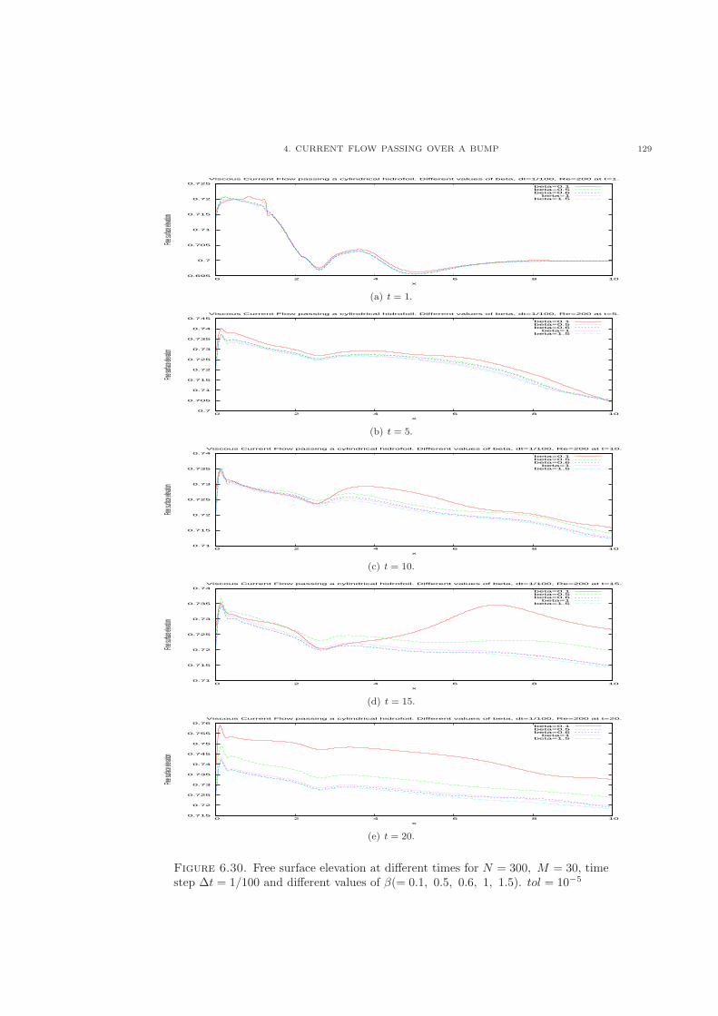
4. CURRENT FLOW PASSING OVER A BUMP 129
0.695
0.7
0.705
0.71
0.715
0.72
0.725
0 2 4 6 8 10
Free surf
ace elev
ation
x
Viscous Current Flow passing a cylindrical hidrofoil. Different values of beta, dt=1/100, Re=200 at t=1.
beta=0.1beta=0.5beta=0.6
beta=1beta=1.5
(a) t = 1.
0.7
0.705
0.71
0.715
0.72
0.725
0.73
0.735
0.74
0.745
0 2 4 6 8 10
Free surf
ace elev
ation
x
Viscous Current Flow passing a cylindrical hidrofoil. Different values of beta, dt=1/100, Re=200 at t=5.
beta=0.1beta=0.5beta=0.6
beta=1beta=1.5
(b) t = 5.
0.71
0.715
0.72
0.725
0.73
0.735
0.74
0 2 4 6 8 10
Free surf
ace elev
ation
x
Viscous Current Flow passing a cylindrical hidrofoil. Different values of beta, dt=1/100, Re=200 at t=10.
beta=0.1beta=0.5beta=0.6
beta=1beta=1.5
(c) t = 10.
0.71
0.715
0.72
0.725
0.73
0.735
0.74
0 2 4 6 8 10
Free surf
ace elev
ation
x
Viscous Current Flow passing a cylindrical hidrofoil. Different values of beta, dt=1/100, Re=200 at t=15.
beta=0.1beta=0.5beta=0.6
beta=1beta=1.5
(d) t = 15.
0.715
0.72
0.725
0.73
0.735
0.74
0.745
0.75
0.755
0.76
0 2 4 6 8 10
Free surf
ace elev
ation
x
Viscous Current Flow passing a cylindrical hidrofoil. Different values of beta, dt=1/100, Re=200 at t=20.
beta=0.1beta=0.5beta=0.6
beta=1beta=1.5
(e) t = 20.
Figure 6.30. Free surface elevation at different times for N = 300, M = 30, timestep Δt = 1/100 and different values of �(= 0.1, 0.5, 0.6, 1, 1.5). tol = 10−5
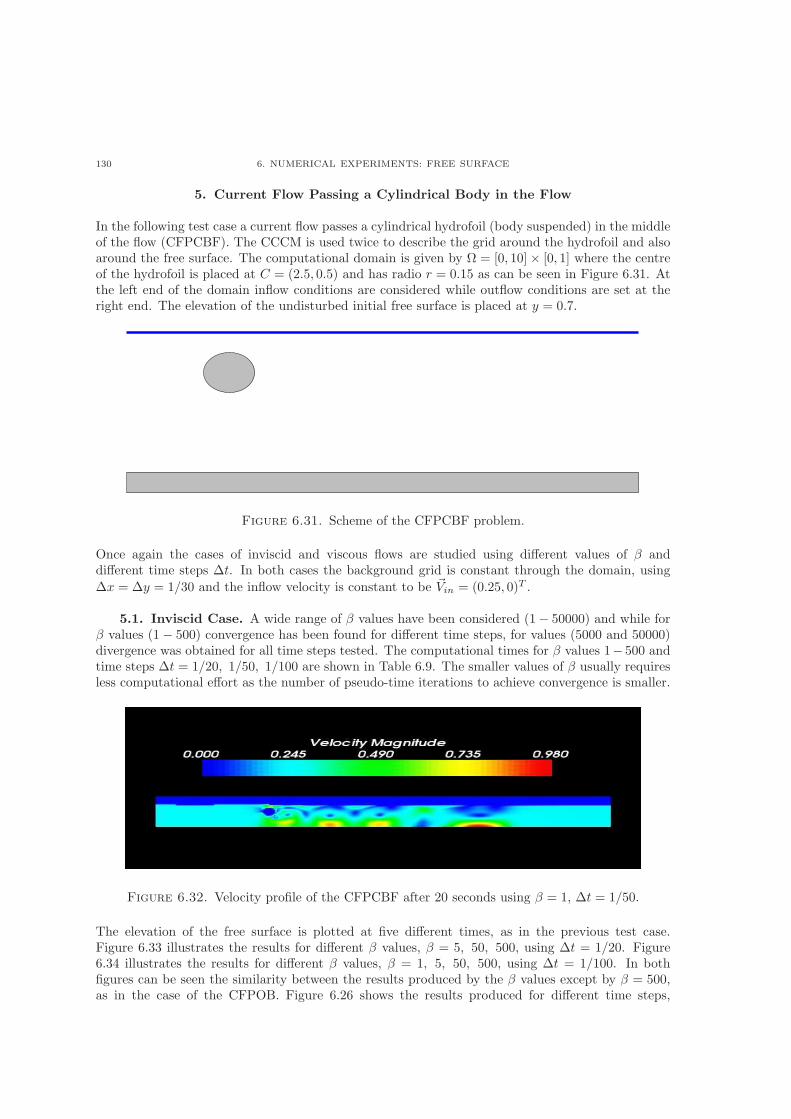
130 6. NUMERICAL EXPERIMENTS: FREE SURFACE
5. Current Flow Passing a Cylindrical Body in the Flow
In the following test case a current flow passes a cylindrical hydrofoil (body suspended) in the middleof the flow (CFPCBF). The CCCM is used twice to describe the grid around the hydrofoil and alsoaround the free surface. The computational domain is given by Ω = [0, 10]× [0, 1] where the centreof the hydrofoil is placed at C = (2.5, 0.5) and has radio r = 0.15 as can be seen in Figure 6.31. Atthe left end of the domain inflow conditions are considered while outflow conditions are set at theright end. The elevation of the undisturbed initial free surface is placed at y = 0.7.
Figure 6.31. Scheme of the CFPCBF problem.
Once again the cases of inviscid and viscous flows are studied using different values of � anddifferent time steps Δt. In both cases the background grid is constant through the domain, using
Δx = Δy = 1/30 and the inflow velocity is constant to be Vin = (0.25, 0)T .
5.1. Inviscid Case. A wide range of � values have been considered (1− 50000) and while for� values (1− 500) convergence has been found for different time steps, for values (5000 and 50000)divergence was obtained for all time steps tested. The computational times for � values 1− 500 andtime steps Δt = 1/20, 1/50, 1/100 are shown in Table 6.9. The smaller values of � usually requiresless computational effort as the number of pseudo-time iterations to achieve convergence is smaller.
Figure 6.32. Velocity profile of the CFPCBF after 20 seconds using � = 1, Δt = 1/50.
The elevation of the free surface is plotted at five different times, as in the previous test case.Figure 6.33 illustrates the results for different � values, � = 5, 50, 500, using Δt = 1/20. Figure6.34 illustrates the results for different � values, � = 1, 5, 50, 500, using Δt = 1/100. In bothfigures can be seen the similarity between the results produced by the � values except by � = 500,as in the case of the CFPOB. Figure 6.26 shows the results produced for different time steps,
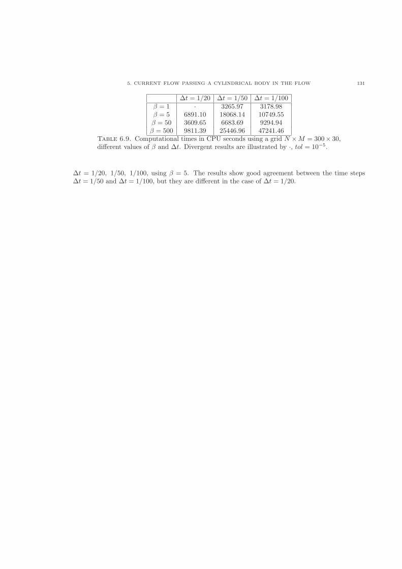
5. CURRENT FLOW PASSING A CYLINDRICAL BODY IN THE FLOW 131
Δt = 1/20 Δt = 1/50 Δt = 1/100� = 1 ⋅ 3265.97 3178.98� = 5 6891.10 18068.14 10749.55� = 50 3609.65 6683.69 9294.94� = 500 9811.39 25446.96 47241.46
Table 6.9. Computational times in CPU seconds using a grid N ×M = 300× 30,different values of � and Δt. Divergent results are illustrated by ⋅, tol = 10−5.
Δt = 1/20, 1/50, 1/100, using � = 5. The results show good agreement between the time stepsΔt = 1/50 and Δt = 1/100, but they are different in the case of Δt = 1/20.
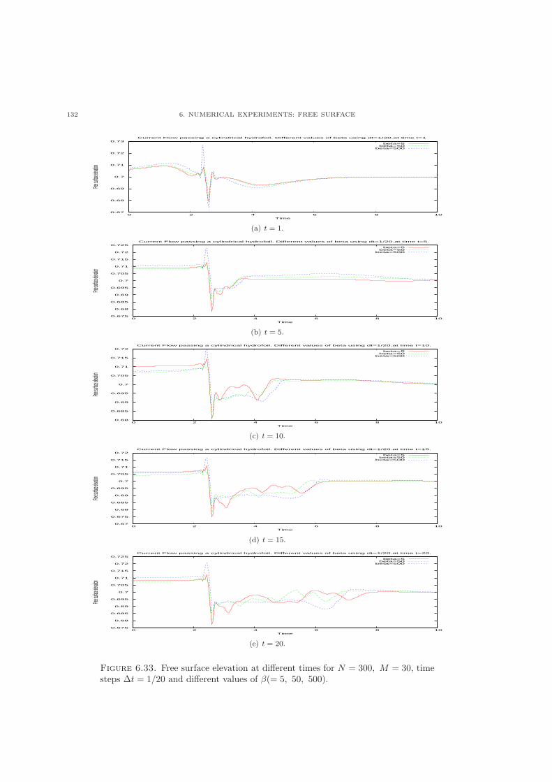
132 6. NUMERICAL EXPERIMENTS: FREE SURFACE
0.67
0.68
0.69
0.7
0.71
0.72
0.73
0 2 4 6 8 10
Free surf
ace elev
ation
Time
Current Flow passing a cylindrical hydrofoil. Different values of beta using dt=1/20.at time t=1
beta=5beta=50
beta=500
(a) t = 1.
0.675
0.68
0.685
0.69
0.695
0.7
0.705
0.71
0.715
0.72
0.725
0 2 4 6 8 10
Free surf
ace elev
ation
Time
Current Flow passing a cylindrical hydrofoil. Different values of beta using dt=1/20.at time t=5.
beta=5beta=50
beta=500
(b) t = 5.
0.68
0.685
0.69
0.695
0.7
0.705
0.71
0.715
0.72
0 2 4 6 8 10
Free surf
ace elev
ation
Time
Current Flow passing a cylindrical hydrofoil. Different values of beta using dt=1/20.at time t=10.
beta=5beta=50
beta=500
(c) t = 10.
0.67
0.675
0.68
0.685
0.69
0.695
0.7
0.705
0.71
0.715
0.72
0 2 4 6 8 10
Free surf
ace elev
ation
Time
Current Flow passing a cylindrical hydrofoil. Different values of beta using dt=1/20.at time t=15.
beta=5beta=50
beta=500
(d) t = 15.
0.675
0.68
0.685
0.69
0.695
0.7
0.705
0.71
0.715
0.72
0.725
0 2 4 6 8 10
Free surf
ace elev
ation
Time
Current Flow passing a cylindrical hydrofoil. Different values of beta using dt=1/20.at time t=20.
beta=5beta=50
beta=500
(e) t = 20.
Figure 6.33. Free surface elevation at different times for N = 300, M = 30, timesteps Δt = 1/20 and different values of �(= 5, 50, 500).
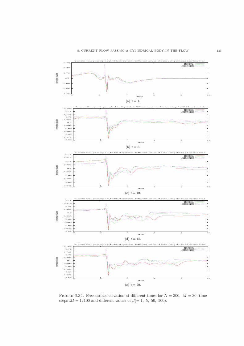
5. CURRENT FLOW PASSING A CYLINDRICAL BODY IN THE FLOW 133
0.67
0.68
0.69
0.7
0.71
0.72
0.73
0 2 4 6 8 10
Free surf
ace elev
ation
Time
Current Flow passing a cylindrical hydrofoil. Different values of beta using dt=1/100.at time t=1.
beta=1beta=5
beta=50beta=500
(a) t = 1.
0.67
0.675
0.68
0.685
0.69
0.695
0.7
0.705
0.71
0.715
0.72
0.725
0 2 4 6 8 10
Free surf
ace elev
ation
Time
Current Flow passing a cylindrical hydrofoil. Different values of beta using dt=1/100.at time t=5.
beta=1beta=5
beta=50beta=500
(b) t = 5.
0.675
0.68
0.685
0.69
0.695
0.7
0.705
0.71
0.715
0.72
0 2 4 6 8 10
Free surf
ace elev
ation
Time
Current Flow passing a cylindrical hydrofoil. Different values of beta using dt=1/100.at time t=10.
beta=1beta=5
beta=50beta=500
(c) t = 10.
0.67
0.675
0.68
0.685
0.69
0.695
0.7
0.705
0.71
0.715
0.72
0 2 4 6 8 10
Free surf
ace elev
ation
Time
Current Flow passing a cylindrical hydrofoil. Different values of beta using dt=1/100.at time t=15.
beta=1beta=5
beta=50beta=500
(d) t = 15.
0.67
0.675
0.68
0.685
0.69
0.695
0.7
0.705
0.71
0.715
0.72
0.725
0 2 4 6 8 10
Free surf
ace elev
ation
Time
Current Flow passing a cylindrical hydrofoil. Different values of beta using dt=1/100.at time t=20.
beta=1beta=5
beta=50beta=500
(e) t = 20.
Figure 6.34. Free surface elevation at different times for N = 300, M = 30, timesteps Δt = 1/100 and different values of �(= 1, 5, 50, 500).
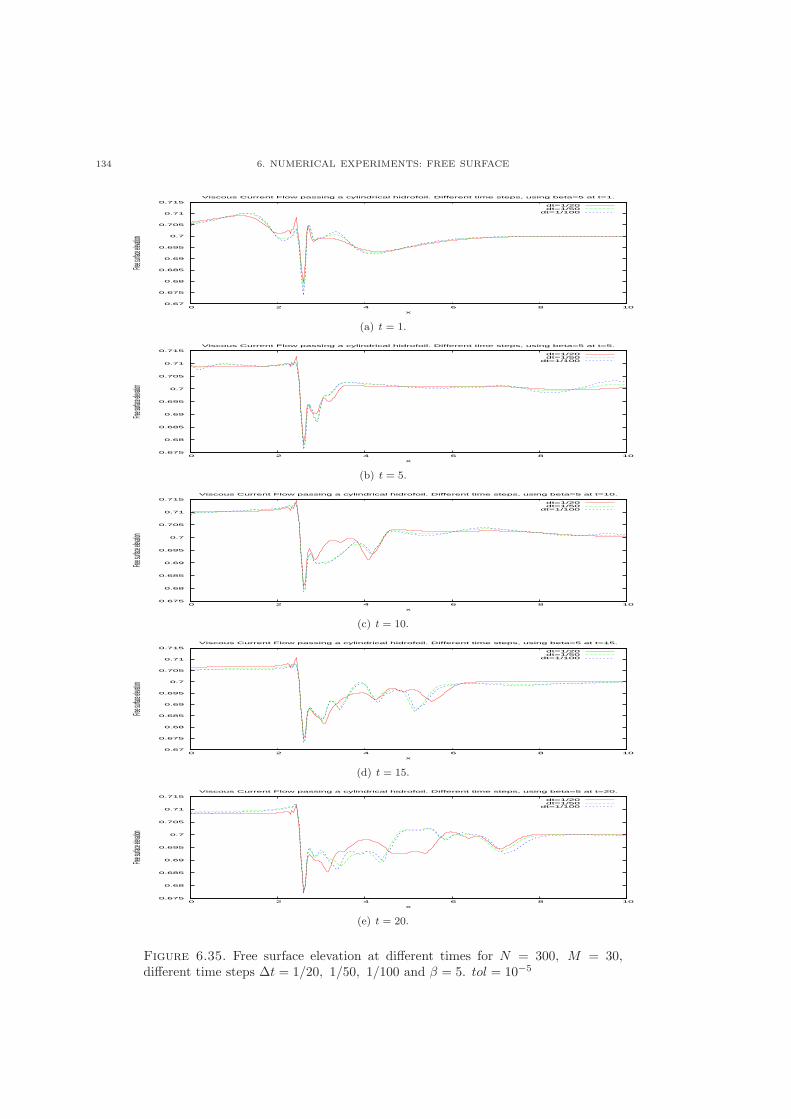
134 6. NUMERICAL EXPERIMENTS: FREE SURFACE
0.67
0.675
0.68
0.685
0.69
0.695
0.7
0.705
0.71
0.715
0 2 4 6 8 10
Free surf
ace elev
ation
x
Viscous Current Flow passing a cylindrical hidrofoil. Different time steps, using beta=5 at t=1.
dt=1/20dt=1/50
dt=1/100
(a) t = 1.
0.675
0.68
0.685
0.69
0.695
0.7
0.705
0.71
0.715
0 2 4 6 8 10
Free surf
ace elev
ation
x
Viscous Current Flow passing a cylindrical hidrofoil. Different time steps, using beta=5 at t=5.
dt=1/20dt=1/50
dt=1/100
(b) t = 5.
0.675
0.68
0.685
0.69
0.695
0.7
0.705
0.71
0.715
0 2 4 6 8 10
Free surf
ace elev
ation
x
Viscous Current Flow passing a cylindrical hidrofoil. Different time steps, using beta=5 at t=10.
dt=1/20dt=1/50
dt=1/100
(c) t = 10.
0.67
0.675
0.68
0.685
0.69
0.695
0.7
0.705
0.71
0.715
0 2 4 6 8 10
Free surf
ace elev
ation
x
Viscous Current Flow passing a cylindrical hidrofoil. Different time steps, using beta=5 at t=15.
dt=1/20dt=1/50
dt=1/100
(d) t = 15.
0.675
0.68
0.685
0.69
0.695
0.7
0.705
0.71
0.715
0 2 4 6 8 10
Free surf
ace elev
ation
x
Viscous Current Flow passing a cylindrical hidrofoil. Different time steps, using beta=5 at t=20.
dt=1/20dt=1/50
dt=1/100
(e) t = 20.
Figure 6.35. Free surface elevation at different times for N = 300, M = 30,different time steps Δt = 1/20, 1/50, 1/100 and � = 5. tol = 10−5
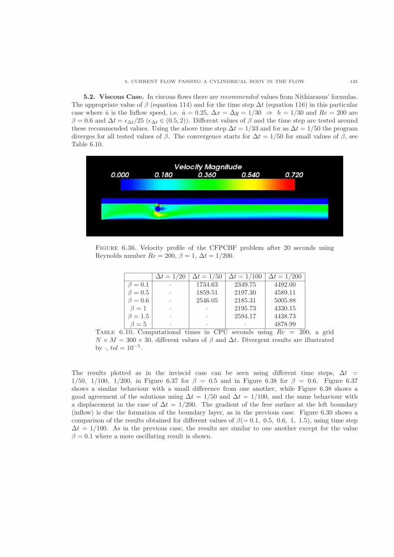
5. CURRENT FLOW PASSING A CYLINDRICAL BODY IN THE FLOW 135
5.2. Viscous Case. In viscous flows there are recommended values from Nithiarasus’ formulas.The appropriate value of � (equation 114) and for the time step Δt (equation 116) in this particularcase where u is the Inflow speed, i.e. u = 0.25, Δx = Δy = 1/30 ⇒ ℎ = 1/30 and Re = 200 are� = 0.6 and Δt = �Δt/25 (�Δt ∈ (0.5, 2)). Different values of � and the time step are tested aroundthese recommended values. Using the above time step Δt = 1/33 and for as Δt = 1/50 the programdiverges for all tested values of �. The convergence starts for Δt = 1/50 for small values of �, seeTable 6.10.
Figure 6.36. Velocity profile of the CFPCBF problem after 20 seconds usingReynolds number Re = 200, � = 1, Δt = 1/200.
Δt = 1/20 Δt = 1/50 Δt = 1/100 Δt = 1/200� = 0.1 ⋅ 1734.63 2349.75 4492.00� = 0.5 ⋅ 1859.51 2197.30 4589.11� = 0.6 ⋅ 2546.05 2185.31 5005.88� = 1 ⋅ ⋅ 2195.73 4330.15� = 1.5 ⋅ ⋅ 2594.17 4438.73� = 5 ⋅ ⋅ ⋅ 4878.99
Table 6.10. Computational times in CPU seconds using Re = 200, a gridN ×M = 300 × 30, different values of � and Δt. Divergent results are illustratedby ⋅, tol = 10−5.
The results plotted as in the inviscid case can be seen using different time steps, Δt =1/50, 1/100, 1/200, in Figure 6.37 for � = 0.5 and in Figure 6.38 for � = 0.6. Figure 6.37shows a similar behaviour with a small difference from one another, while Figure 6.38 shows agood agreement of the solutions using Δt = 1/50 and Δt = 1/100, and the same behaviour witha displacement in the case of Δt = 1/200. The gradient of the free surface at the left boundary(inflow) is due the formation of the boundary layer, as in the previous case. Figure 6.30 shows acomparison of the results obtained for different values of �(= 0.1, 0.5, 0.6, 1, 1.5), using time stepΔt = 1/100. As in the previous case, the results are similar to one another except for the value� = 0.1 where a more oscillating result is shown.
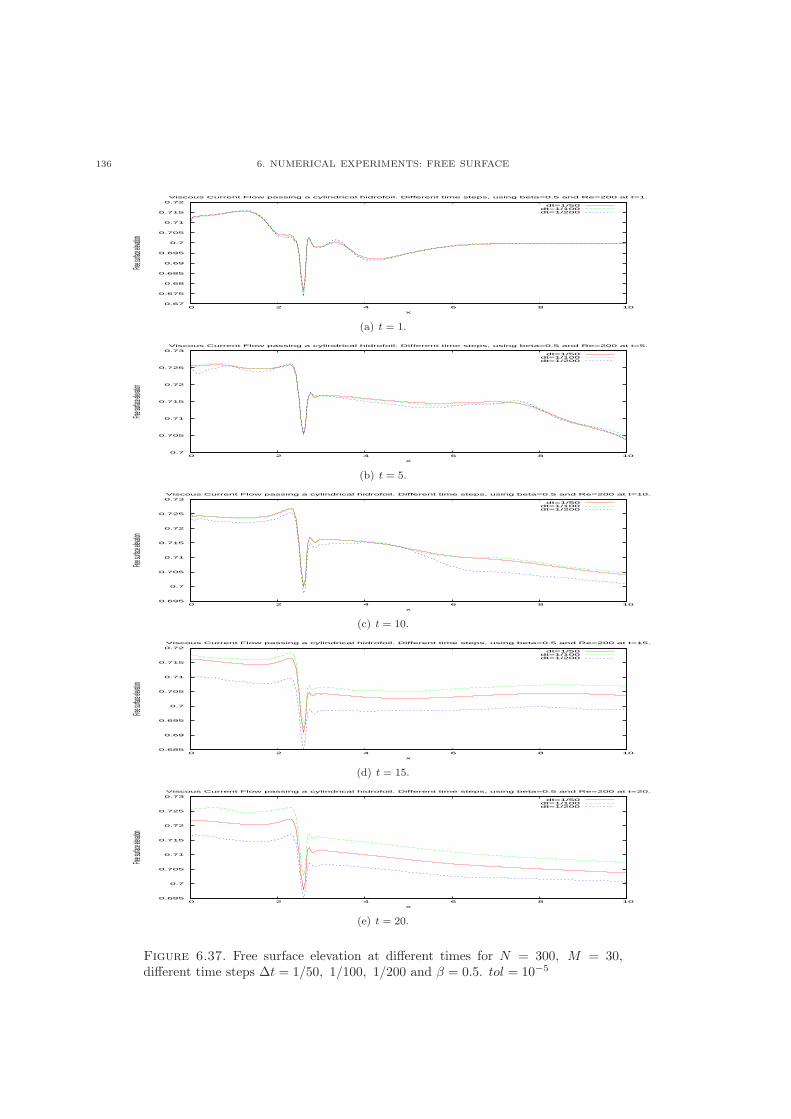
136 6. NUMERICAL EXPERIMENTS: FREE SURFACE
0.67
0.675
0.68
0.685
0.69
0.695
0.7
0.705
0.71
0.715
0.72
0 2 4 6 8 10
Free surf
ace elev
ation
x
Viscous Current Flow passing a cylindrical hidrofoil. Different time steps, using beta=0.5 and Re=200 at t=1.
dt=1/50dt=1/100dt=1/200
(a) t = 1.
0.7
0.705
0.71
0.715
0.72
0.725
0.73
0 2 4 6 8 10
Free surf
ace elev
ation
x
Viscous Current Flow passing a cylindrical hidrofoil. Different time steps, using beta=0.5 and Re=200 at t=5.
dt=1/50dt=1/100dt=1/200
(b) t = 5.
0.695
0.7
0.705
0.71
0.715
0.72
0.725
0.73
0 2 4 6 8 10
Free surf
ace elev
ation
x
Viscous Current Flow passing a cylindrical hidrofoil. Different time steps, using beta=0.5 and Re=200 at t=10.
dt=1/50dt=1/100dt=1/200
(c) t = 10.
0.685
0.69
0.695
0.7
0.705
0.71
0.715
0.72
0 2 4 6 8 10
Free surf
ace elev
ation
x
Viscous Current Flow passing a cylindrical hidrofoil. Different time steps, using beta=0.5 and Re=200 at t=15.
dt=1/50dt=1/100dt=1/200
(d) t = 15.
0.695
0.7
0.705
0.71
0.715
0.72
0.725
0.73
0 2 4 6 8 10
Free surf
ace elev
ation
x
Viscous Current Flow passing a cylindrical hidrofoil. Different time steps, using beta=0.5 and Re=200 at t=20.
dt=1/50dt=1/100dt=1/200
(e) t = 20.
Figure 6.37. Free surface elevation at different times for N = 300, M = 30,different time steps Δt = 1/50, 1/100, 1/200 and � = 0.5. tol = 10−5
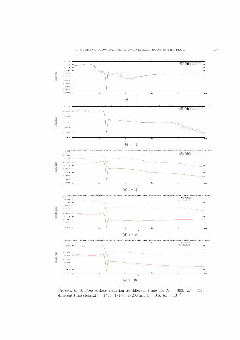
5. CURRENT FLOW PASSING A CYLINDRICAL BODY IN THE FLOW 137
0.67
0.675
0.68
0.685
0.69
0.695
0.7
0.705
0.71
0.715
0.72
0 2 4 6 8 10
Free surf
ace elev
ation
x
Viscous Current Flow passing a cylindrical hidrofoil. Different time steps, using beta=0.6 and Re=200 at t=1.
dt=1/50dt=1/100dt=1/200
(a) t = 1.
0.7
0.705
0.71
0.715
0.72
0.725
0.73
0 2 4 6 8 10
Free surf
ace elev
ation
x
Viscous Current Flow passing a cylindrical hidrofoil. Different time steps, using beta=0.6 and Re=200 at t=5.
dt=1/50dt=1/100dt=1/200
(b) t = 5.
0.695
0.7
0.705
0.71
0.715
0.72
0.725
0.73
0.735
0.74
0 2 4 6 8 10
Free surf
ace elev
ation
x
Viscous Current Flow passing a cylindrical hidrofoil. Different time steps, using beta=0.6 and Re=200 at t=10.
dt=1/50dt=1/100dt=1/200
(c) t = 10.
0.69
0.695
0.7
0.705
0.71
0.715
0.72
0.725
0.73
0.735
0.74
0.745
0 2 4 6 8 10
Free surf
ace elev
ation
x
Viscous Current Flow passing a cylindrical hidrofoil. Different time steps, using beta=0.6 and Re=200 at t=15.
dt=1/50dt=1/100dt=1/200
(d) t = 15.
0.695
0.7
0.705
0.71
0.715
0.72
0.725
0.73
0.735
0.74
0 2 4 6 8 10
Free surf
ace elev
ation
x
Viscous Current Flow passing a cylindrical hidrofoil. Different time steps, using beta=0.6 and Re=200 at t=20.
dt=1/50dt=1/100dt=1/200
(e) t = 20.
Figure 6.38. Free surface elevation at different times for N = 300, M = 30,different time steps Δt = 1/50, 1/100, 1/200 and � = 0.6. tol = 10−5
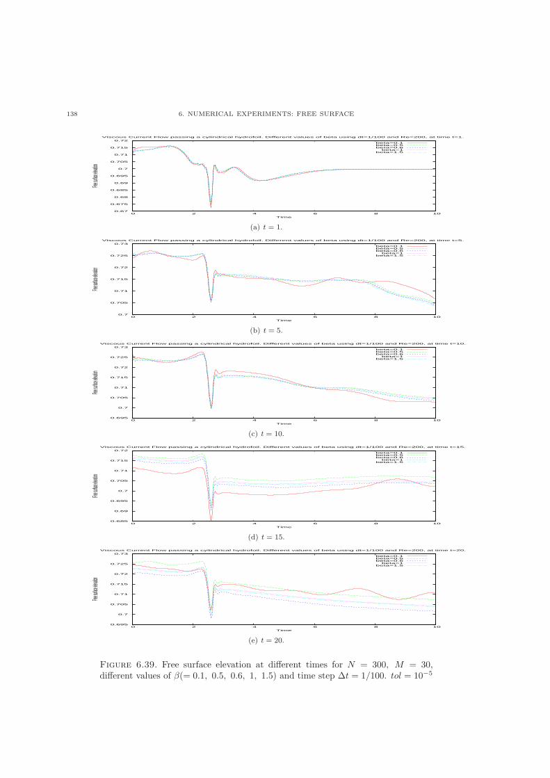
138 6. NUMERICAL EXPERIMENTS: FREE SURFACE
0.67
0.675
0.68
0.685
0.69
0.695
0.7
0.705
0.71
0.715
0.72
0 2 4 6 8 10
Free surf
ace elev
ation
Time
Viscous Current Flow passing a cylindrical hydrofoil. Different values of beta using dt=1/100 and Re=200, at time t=1.
beta=0.1beta=0.5beta=0.6
beta=1beta=1.5
(a) t = 1.
0.7
0.705
0.71
0.715
0.72
0.725
0.73
0 2 4 6 8 10
Free surf
ace elev
ation
Time
Viscous Current Flow passing a cylindrical hydrofoil. Different values of beta using dt=1/100 and Re=200, at time t=5.
beta=0.1beta=0.5beta=0.6
beta=1beta=1.5
(b) t = 5.
0.695
0.7
0.705
0.71
0.715
0.72
0.725
0.73
0 2 4 6 8 10
Free surf
ace elev
ation
Time
Viscous Current Flow passing a cylindrical hydrofoil. Different values of beta using dt=1/100 and Re=200, at time t=10.
beta=0.1beta=0.5beta=0.6
beta=1beta=1.5
(c) t = 10.
0.685
0.69
0.695
0.7
0.705
0.71
0.715
0.72
0 2 4 6 8 10
Free surf
ace elev
ation
Time
Viscous Current Flow passing a cylindrical hydrofoil. Different values of beta using dt=1/100 and Re=200, at time t=15.
beta=0.1beta=0.5beta=0.6
beta=1beta=1.5
(d) t = 15.
0.695
0.7
0.705
0.71
0.715
0.72
0.725
0.73
0 2 4 6 8 10
Free surf
ace elev
ation
Time
Viscous Current Flow passing a cylindrical hydrofoil. Different values of beta using dt=1/100 and Re=200, at time t=20.
beta=0.1beta=0.5beta=0.6
beta=1beta=1.5
(e) t = 20.
Figure 6.39. Free surface elevation at different times for N = 300, M = 30,different values of �(= 0.1, 0.5, 0.6, 1, 1.5) and time step Δt = 1/100. tol = 10−5
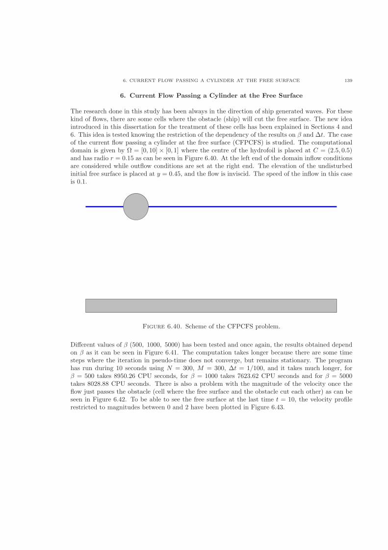
6. CURRENT FLOW PASSING A CYLINDER AT THE FREE SURFACE 139
6. Current Flow Passing a Cylinder at the Free Surface
The research done in this study has been always in the direction of ship generated waves. For thesekind of flows, there are some cells where the obstacle (ship) will cut the free surface. The new ideaintroduced in this dissertation for the treatment of these cells has been explained in Sections 4 and6. This idea is tested knowing the restriction of the dependency of the results on � and Δt. The caseof the current flow passing a cylinder at the free surface (CFPCFS) is studied. The computationaldomain is given by Ω = [0, 10] × [0, 1] where the centre of the hydrofoil is placed at C = (2.5, 0.5)and has radio r = 0.15 as can be seen in Figure 6.40. At the left end of the domain inflow conditionsare considered while outflow conditions are set at the right end. The elevation of the undisturbedinitial free surface is placed at y = 0.45, and the flow is inviscid. The speed of the inflow in this caseis 0.1.
Figure 6.40. Scheme of the CFPCFS problem.
Different values of � (500, 1000, 5000) has been tested and once again, the results obtained dependon � as it can be seen in Figure 6.41. The computation takes longer because there are some timesteps where the iteration in pseudo-time does not converge, but remains stationary. The programhas run during 10 seconds using N = 300, M = 300, Δt = 1/100, and it takes much longer, for� = 500 takes 8950.26 CPU seconds, for � = 1000 takes 7623.62 CPU seconds and for � = 5000takes 8028.88 CPU seconds. There is also a problem with the magnitude of the velocity once theflow just passes the obstacle (cell where the free surface and the obstacle cut each other) as can beseen in Figure 6.42. To be able to see the free surface at the last time t = 10, the velocity profilerestricted to magnitudes between 0 and 2 have been plotted in Figure 6.43.
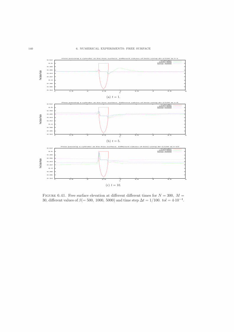
140 6. NUMERICAL EXPERIMENTS: FREE SURFACE
0.34
0.36
0.38
0.4
0.42
0.44
0.46
0.48
0.5
0.52
1 1.5 2 2.5 3 3.5 4 4.5 5
Free Sur
face Pos
ition
x
Flow passing a cylinder at the free surface. Different values of beta using dt=1/100 at t=1
Cylinderbeta=500
beta=1000beta=5000
(a) t = 1.
0.34
0.36
0.38
0.4
0.42
0.44
0.46
0.48
0.5
0.52
1 1.5 2 2.5 3 3.5 4 4.5 5
Free Sur
face Pos
ition
x
Flow passing a cylinder at the free surface. Different values of beta using dt=1/100 at t=5
Cylinderbeta=500
beta=1000beta=5000
(b) t = 5.
0.34
0.36
0.38
0.4
0.42
0.44
0.46
0.48
0.5
0.52
1 1.5 2 2.5 3 3.5 4 4.5 5
Free Sur
face Pos
ition
x
Flow passing a cylinder at the free surface. Different values of beta using dt=1/100 at t=10
Cylinderbeta=500
beta=1000beta=5000
(c) t = 10.
Figure 6.41. Free surface elevation at different different times for N = 300, M =30, different values of �(= 500, 1000, 5000) and time step Δt = 1/100. tol = 4⋅10−4.
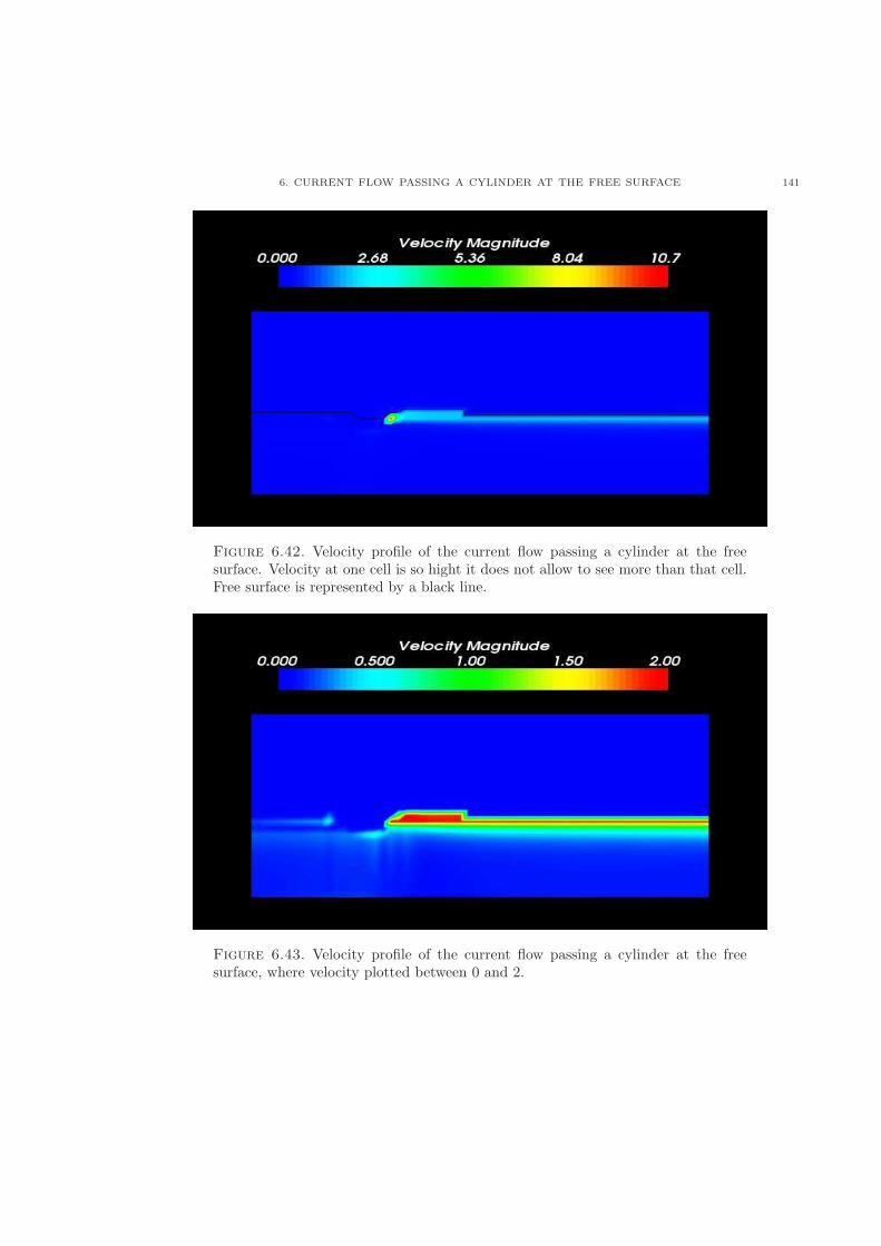
6. CURRENT FLOW PASSING A CYLINDER AT THE FREE SURFACE 141
Figure 6.42. Velocity profile of the current flow passing a cylinder at the freesurface. Velocity at one cell is so hight it does not allow to see more than that cell.Free surface is represented by a black line.
Figure 6.43. Velocity profile of the current flow passing a cylinder at the freesurface, where velocity plotted between 0 and 2.

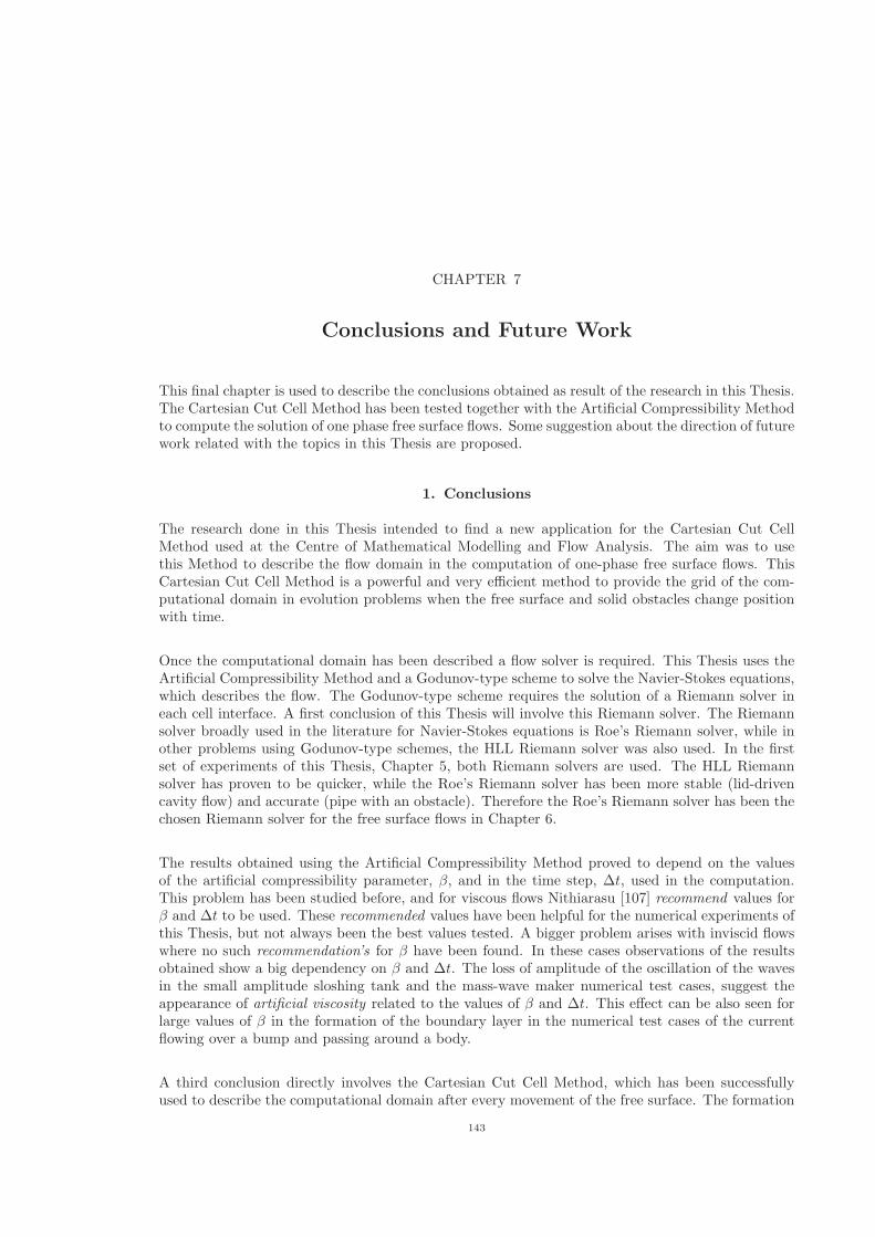
CHAPTER 7
Conclusions and Future Work
This final chapter is used to describe the conclusions obtained as result of the research in this Thesis.The Cartesian Cut Cell Method has been tested together with the Artificial Compressibility Methodto compute the solution of one phase free surface flows. Some suggestion about the direction of futurework related with the topics in this Thesis are proposed.
1. Conclusions
The research done in this Thesis intended to find a new application for the Cartesian Cut CellMethod used at the Centre of Mathematical Modelling and Flow Analysis. The aim was to usethis Method to describe the flow domain in the computation of one-phase free surface flows. ThisCartesian Cut Cell Method is a powerful and very efficient method to provide the grid of the com-putational domain in evolution problems when the free surface and solid obstacles change positionwith time.
Once the computational domain has been described a flow solver is required. This Thesis uses theArtificial Compressibility Method and a Godunov-type scheme to solve the Navier-Stokes equations,which describes the flow. The Godunov-type scheme requires the solution of a Riemann solver ineach cell interface. A first conclusion of this Thesis will involve this Riemann solver. The Riemannsolver broadly used in the literature for Navier-Stokes equations is Roe’s Riemann solver, while inother problems using Godunov-type schemes, the HLL Riemann solver was also used. In the firstset of experiments of this Thesis, Chapter 5, both Riemann solvers are used. The HLL Riemannsolver has proven to be quicker, while the Roe’s Riemann solver has been more stable (lid-drivencavity flow) and accurate (pipe with an obstacle). Therefore the Roe’s Riemann solver has been thechosen Riemann solver for the free surface flows in Chapter 6.
The results obtained using the Artificial Compressibility Method proved to depend on the valuesof the artificial compressibility parameter, �, and in the time step, Δt, used in the computation.This problem has been studied before, and for viscous flows Nithiarasu [107] recommend values for� and Δt to be used. These recommended values have been helpful for the numerical experiments ofthis Thesis, but not always been the best values tested. A bigger problem arises with inviscid flowswhere no such recommendation’s for � have been found. In these cases observations of the resultsobtained show a big dependency on � and Δt. The loss of amplitude of the oscillation of the wavesin the small amplitude sloshing tank and the mass-wave maker numerical test cases, suggest theappearance of artificial viscosity related to the values of � and Δt. This effect can be also seen forlarge values of � in the formation of the boundary layer in the numerical test cases of the currentflowing over a bump and passing around a body.
A third conclusion directly involves the Cartesian Cut Cell Method, which has been successfullyused to describe the computational domain after every movement of the free surface. The formation
143
144 7. CONCLUSIONS AND FUTURE WORK
of the grid was very efficient as only a few cells were affected after every movement of the free surfaceor moving body. This method has some restrictions that have been already considered in the designof the numerical experiment used, as in the semi dam break problem. The merging and de-merging(splitting) technique used made the transition between flow and solid cells smooth.
The Height Function Method to move the free surface has produced accurate and quick results.However, the problem of the dependency of these results on � and Δt values does not allow themto be judged effectively.
While in the 1-phase flow the computation of the flow over a bump takes around 3 hours usingN = 300, M = 30, the 2-phase flow takes takes between 4 and 5 days using N = 200, M = 50. Inthe 2-phase flow the time step used is around 10−5, while in this Thesis values around 10−2 wereused. As it was expected the time step used in the computation of the 1-phase flow is much biggerthan the used in the is much 2-phase flow and as consequence the computational cost is much smallerin the 1-phase case.
The final conclusion based on the results obtained in this Thesis is that the Artificial CompressibilityMethod, as applied in this Thesis, is not an appropriate flow solver to use with the Cartesian CutCell and the Height Function Methods. On the other hand, the Cartesian Cut Cell Method togetherwith the Height Function Method seems to be a suitable and efficient method to study the 1-phasefree surface flows, using a suitable flow solver.
2. Future Work
There are different methods used in this Thesis, and therefore there are many ways of extendingthe research done maintaining the spirit of finding applications for the use of the Cartesian Cut CellMethod.
The first and obvious possibility of study based in the results of this Thesis, is to try the CartesianCut Cell and the Height Function Methods using different flow solvers, see Section 5. The resultsin this Thesis have already influenced current work in this direction.
The Artificial Compressibility Method applied in the fashion of this Thesis has produced resultswhich depend in the artificial compressibility parameter, � and the time step, Δt. The question ofhow to avoid dependency and/or obtain recommended values of � and Δt for inviscid flowsremains open and is a possible area of future work.
The Height Function Method has been used for the movement of the free surface. Extensions of thiswork can be done using different methods to move the free surface, see Chapter 4 Section 2,for the Interface Capturing Methods, and Section 3, for the Interface Tracking Methods.
The Cartesian Cut Cell Method can also be extended. An extension could be to use an AdaptiveMesh Refinement in the background Cartesian grid, i.e., be able to use smaller backgroundcells around the boundaries, obstacles or/and free surface, and bigger cells away from the bound-aries. Better resolution around boundary cells would be obtained.
2. FUTURE WORK 145
The merging cell technique in the case of 1-phase free surface flows presents a problem, shown inFigure 2.13. To avoid this problem in this Thesis, a convention has been taken: free surface needingto be merged, will be merged with the cell below. Due this convention, the full dam break problemcan not be studied, and it was replaced by the semi dam break problem. Research to avoid thisproblem remains to be done.
The idea of ship generated waves has just been introduced in this Thesis. Research will be needed inthis direction for cells where the free surface and the obstacle (ship) cut each other. Theapplications of this study will not be limited to ship generated waves, but all related applicationswith bodies cutting the free surface as for example oil platforms, wave energy devices and fishing nets.
Extension to three dimensions will be always the final goal in the research of free surface flows.

List of References
[1] Alinghi Team’s web page.http://www.alinghi.com.
[2] CFX Ansys.http://www.ansys.com/Products/cfx.asp.
[3] Clay mathematics institute.http://www.claymath.org/millennium/Navier-Stokes Equations/.
[4] Fluent inc.http://www.fluent.com/.
[5] MIKE by DHI.http://www.dhigroup.com/.
[6] Modelling and Scientific Computing. Ecole Polytechnique Federale de Lausanne.http://iacs.epfl.ch/cmcs/NewResearch/americascup2003.php3.
[7] Nextlimit’s web.http://www.nextlimit.com.
[8] Ship Technology Department, MARINTEK, SINTEF.http://www.sintef.no/content/page3.aspx?id=13406.
[9] Harwell Subroutine Library.http://www.cse.clrc.ac.uk/nag/hsl/, 2006.
[10] J. A. Armesto Alvarez. Lattice Boltzmann Equation in Curvilinear Domain. Master Thesis,Technischen Universitat Kaiserslautern, September 2003.
[11] J. A. Armesto Alvarez, C. G. Mingham, D. M. Causon, L. Quian, and D. M. Ingam. Studyof two different Riemann solvers for the lid-driven Cavity Flow. Short communication,International Congress of Mathematicians, Madrid, Spain, 2006.
[12] D. Apsley and W. Hu. Cfd simulation of two- and three-dimensional free-surface flow.International Journal for Numerical Methods is Fluids, 42:465–491, 2003.
[13] R. Azcueta. Turbulent Free-Surface Flows Around Ships and Floating Bodies. PhD thesis,Technischen Universitat Hamburg-Harburg, July 2001.
[14] G.K. Batchelor. An Introduction to Fluid Dynamics. Cambridge Mathematical Library, 1967.[15] P. Batten, M. A. Leschziner, and U. C. Goldberg. Average-State Jacobians and Implicit
Methods for Compressible Viscous and Turbulent Flows. Journal of Computational Physics,137:38–78, 1997.
[16] F. Bet, D. Hanel, and S. D. Sharma. Numerical Simulation of Ship Flow by a Method ofArtificial Compressibility. In Proceedings of the 22nd Symposium on Naval Hydrodynamics,2000.
[17] F. Bet, N. Stuntz, D. Hanel, and S. D. Sharma. Numerical Simulation of Ship Flow inRestricted Water. In Proceedings of the 7tℎ International Conference on Numerical ShipHydrodynamics, 1999.
[18] J. V. Boussinesq. Theorie des ondes et des remous qui se propaent le long d’un canalrectangulaire horizontal, en communiquant au liquide contenu dans ce canal des vitessessensiblement pareilles de la surface au dond. J. Math. Pures Appliq, 17:55–108, 1872.
147
148 List of References
[19] G. Cerne, S. Petelin, and I. Tiselj. Numerical errors of the volume-of-fluid interface trackingalgorithm. International Journal in Numerical Methods in Fluids, 38:329–350, 2002.
[20] P. M. Carrica, R. V. Wilson, and F. Stern. Single-phase level set method for unsteady viscousfree flows. In G. Buscaglia, E. Dari, and O. Zamonsky, editors, Mecanica ComputacionalVolumen XXIII, volume 62, pages 1613–1631. Kluwer Academic Publishers, Bariloche,Argentina, 2004.
[21] P. M. Carrica, R. V. Wilson, and F. Stern. An unsteady single-phase level set method forviscous free surface flows. International Journal for Numerical Methods in Fluids, 53(2):229–256, 2006.
[22] M. J. Castro, J. A. Garcıa-Rodrıguez, J. M. Gonzalez-Vida, J. Macıas, C. Pares, and M. E.Vazquez-Cendon. Numerical simulation of two-layer shallow water flows through channels withirregular geometry. Journal of Computational Physics, 195:202–235, 2004.
[23] M. J. Castro, J. Macıas, and C. Pares. A q-scheme for a class of systems of coupled conservationlaws with source term. application to a two-layer 1d shallow water system. ESAIM-Math ModelNum, 1(35):107–127, 2001.
[24] D. M. Causon, D. M. Ingram, and C. G. Mingham. A Cartesian cut cell method for shallowwater flows with moving boundaries. Advances in Water Resources, 24:899–911, 2001.
[25] D. M. Causon, D. M. Ingram, C. G. Mingham, G. Yang, and R. V. Pearson. Calculationof shallow water flows using a Cartesian cut cell approach. Advances in Water Resources,23:545–562, 2000.
[26] M. A. Celigueta, E. Onate, and S. Idelsohn. Simulation of Skip Sinking Simulations withthe Particle Finite Element Method. In E. Onate, J. Garcıa, P. Bergan, and T. Kvamsdal,editors, Computational Methods in Marine Engineering II, pages 89–92. International Centerfor Numerical Methods in Engineering (CIMNE), Barcelona, Spain, 2007.
[27] C. T. Chan and K. Anastasiou. Solution of incompressible flows with or without a free surfaceusing the finite volume method on unstructures triangular meshes. International Journal forNumerical Methods in Fluids, 29:35–57, 1999.
[28] R.-Y. Chang and W.-H. Yang. Numerical simulation of mold filling in injection molding usinga three-dimensional finite volume approach. International Journal for Numerical Methods inFluids, 37:125–148, 2001.
[29] H.-C. Chen and K. Yu. Cfd simulations of wave-current-body interactions including greenwaterand wet deck slamming. Computers & Fluids, 10.1016/j.compfluid.2008.01.026, 2008.
[30] A. J. Chorin. Numerical Solution of the navier-stokes equations. Incomprenssible ViscousFlows Problems. Journal of Computational Physics, 2:12–26, 1967. (Reedited in 1997, volume135, pages 118–125).
[31] A. J. Chorin. Numerical Solution of the Navier-Stokes Equations. Mathematics ofComputation, 22:745–762, 1968.
[32] H. H. Chun, I. R. Park, and S. K.Lee. Analysis of Turbulence Free-Surface Flow around Hullsin Shallow Water Channel by a Level-set Method. In Proceedings of the 23nd Symposium onNaval Hydrodynamics, 2001.
[33] A. Colagrossi and G. Colicchio. Investigation of Some Naval Hydrodynamic Problems througha SPH Method. In E. Onate, J. Garcıa, P. Bergan, and T. Kvamsdal, editors, ComputationalMethods in Marine Engineering II, pages 81–84. International Center for Numerical Methodsin Engineering (CIMNE), Barcelona, Spain, 2007.
[34] G. S. de Paulo, M. F. Tome a, and S. McKee. A marker-and-cell approach to viscoelastic freesurface flows using the ptt model. Journal of Non-Newtonian Fluid Mechanics, (147):149–174,2007.
[35] T. Farrant, M. Tan, and W. G. Price. A cell boundary element method applied to laminarvortex shedding from circular cylinders. Computers & Fluids, 30:211–236, 2001.
[36] C. L. Fefferman. Existence and smoothness of the Navier-Stokes equations. Official ProblemDescription, Clay Mathematics Institute.
List of References 149
[37] G. Fekken. Numerical Simulation of Free-Surface Flow with Moving Rigid Bodies. PhD thesis,Rijksuniversiteit Groningen, March 2004.
[38] G. E. Ferrari, M. Politano, and L. Weber. Numerical simulation of free surface flows on a fishbypass. Computers & Fluids, 10.1016/j.compfluid.2008.01.014, 2008.
[39] J. H. Ferziger and M. Peric. Computational methods for fluid dynamics. Springer Verlag, 1996.[40] A. Fortier. Numerical Simulation of Hydrodynamic Bearings with Engineered Slip/No-Slip
Surfaces. PhD thesis, Georgia Institute of Technology, July 2004.[41] J. Garcıa-Espinosa, A. Valls, and Onate. An overlapping domain decomposition level sel
(ODDLS) method for simulation of free surface. In E. Onate, J. Garcıa, P. Bergan,and T. Kvamsdal, editors, Computational Methods in Marine Engineering II, pages 17–23.International Center for Numerical Methods in Engineering (CIMNE), Barcelona, Spain, 2007.
[42] P. Garcıa-Navarro, A. Fras, and I. Villanueva. Dam-break flow simulation: some results forone-dimensional models of real cases. Journal of Hydrology, 216:227–247, 1999.
[43] J. Gerrits. Dynamics of Liquid-Filled Spacecraft. Numerical Simulation of Coupled Solid-LiquidDynamics. PhD thesis, Rijksuniversiteit Groningen, December 2001.
[44] U. Ghia, K. N. Ghia, and C. T. Shin. High-Re Solutions for Incompressible Flows Usingthe Navier-Stokes Equations and a Multigrid Method. Journal of Computational Physics,48:387–411, 1982.
[45] R. A. Gingold and J. J. Monaghan. Smoothed particle hydrodynamics : theory and applicationto non-spherical stars. Monthly Notices of the Royal Astronomical Society , 375., 181:375–389,1977.
[46] G. Gottardi and M. Venutelli. Central scheme for two-dimensional dam-break flow simulation.Advances in Water Resources, 27:259–268, 2004.
[47] A. E. Green, N. Laws, and P. M. Naghdi. On the theory of water waves. Proc. R. Soc. Lond.A., 338:43–55, 1974.
[48] P. A. Gremaud, C. M. Kuster, and Z. Li. A study of numerical methods for the level setapproach. Applied Numerical Mathematics, 57:837–846, 2007.
[49] P. Groenenboom and B. Cartwright. Interaction between Structured and Waves Using theCoupled FE-SPH. In E. Onate, J. Garcıa, P. Bergan, and T. Kvamsdal, editors, ComputationalMethods in Marine Engineering II, pages 77–80. International Center for Numerical Methodsin Engineering (CIMNE), Barcelona, Spain, 2007.
[50] P. L. Bhatnagar E. P. Gross and M. Krook. A Model for Collision Processes in Gases. I. SmallAmplitude Processes in Charged and Neutral One-Component Systems. Physical Review,94:511–525, 1954.
[51] V. Guinot. Godunov-type Schemes: An introduction for engineers. Elsevier Science B. V.,Amsterdam, 2003.
[52] F. H. Harlow and J. E. Welch. Numerical calculation of time-dependent viscous incompressibleflow of fluid with free surface. Physics of Fluids, 8(12):2182–2189, 1965.
[53] A. Harten, P. D. Lax, and B. van Leer. On Upstream Differencing and Godunov-type Schemesfor Hyperbolic Conservation Laws. SIAM Review, 25:35–61, 1983.
[54] D. J. E. Harvie and D. F. Fletcher. A New Volume of Fluid Advection Algorithm. the StreamScheme. Journal of Computational Physics, 162:1–32, 2000.
[55] X. He and G. Doolen. Lattice Boltzmann Method on Curvilinear Coordinates System: Flowaround a Circular Cylinder. Journal of Computational Physics, 134:306–315, 1997.
[56] G. Dıaz Hernandez. Analisis de resolancia portuaria: Generacion, transitoriedad, no linealidady acoplamiento geometrico. PhD thesis, Universidad de Cantabria, March 2006.
[57] C. Hirsch. Numerical Computation of Internal and External Flows. Volume 2: ComputationalMethods for Inviscid and Viscous Flows. Wiley Series in Numerical Methods in Engineering,1990.
[58] C. W. Hirt and B. D. Nichols. Volume of Fluid (VOF) Method for the Dynamics of FreeBoundaries. Journal of Computational Physics, 39:201–225, 1981.
150 List of References
[59] S. Hou, Q. Zou, S. Chen, G. Doolen, and A. C. Cogley. Simulation of cavity flow by the latticeboltzmann method. Journal of Computational Physics, 118:329–347, 1995.
[60] K. Hu, C. G. Mingham, and D. M. Causon. A Bore-Capturing Finite Volume Method forOpen-Channel Flows. International Journal for Numerical Methods in Fluids, 28:1241–1261,1998.
[61] K. Hu, C. G. Mingham, and D. M. Causon. Numerical simulation of wave overtopping ofcoastal structures using the non-linear shallow water equations. Coastal Engineering, 41:433–465, 2000.
[62] W. F. Hughes. An Introduction to Viscous Flows. Hemisphere Publishing Corporation, 1979.[63] D. M. Ingram, D. M. Causon, and C. G. Mingham. Developments in Cartesian cut cell
methods. Mathematics and Computers in Simulation, 61:561–572, 2003.[64] M. J. Castro Dıaz J. Macıas M. E. Vazquez Cendon J. A. Garcıa-Rodrıguez, J. M. Gonzalez-
Vida. Numerical simulation of internal tides in the strait of gibraltar. Revista de laReal Academia de Ciencias Exactas, Fısicas y Naturales. Serie A: Matematicas (RACSAM),96:322–341, 2002.
[65] T. Jiang. Ship Waves in Shallow Water. Fortschritt-Berichte VDI, 2001.[66] T. Jiang, R. Henn, and S. D. Sharma. Wash Waves Generated by Ships Moving on Fairways of
Varying Topography. In Proceedings of the 24tℎ Symposium On Naval Hydrodynamics, pages441–457, 2002.
[67] W. Jiankang and B. Chen. Unsteady ship waves in shallow water of varying depth based onGreen-Naghdi equation. Ocean Engineering, 30:1899–1913, 2003.
[68] J. E. Pilliod Jr. and E.G. Puckett. Second-order accurate volume-of-fluid algorithms fortracking material interfaces. Journal of Computational Physics, 199:465–502, 2004.
[69] M. Kang, B. Merriman, and S. Osher. Numerical simulations for the motion of soap bubblesusing level set methods. Computers & Fluids, 37:524–535, 2008.
[70] T. Kato, S. Kawano, K. Nakahashi, T. Yambe, S. Nitta, and H. Hashimoto. Computationalflow visualization in vibrating flow pump type artificial heart by unstructured grid. ArtificialOrgans, 27(1):41–48, 2003.
[71] F. J. Kelecy and R. H. Pletcher. The Development of a Free Surface Capturing Approach forMultidimensional Free Surface Flows in Closed Containers. Journal of Computational Physics,138:939–980, 1997.
[72] K. M. T. Kleefsman. Water Impact Loading on Offshore Structures. A Numerical Study. PhDthesis, Rijksuniversiteit Groningen, November 2005.
[73] K. M. T. Kleefsman, G. Fekken, A. E. P. Veldman, B. Iwanowski, and B. Buchner. A volume-of-fluid based simulation method for wave impact problems. Journal of Computational Physics,(206):363–393, 2005.
[74] C. Korner, T. Pohl, U. Rude, N. Thurey, and T. Zeiser. Parallel Lattice Boltzmann Methodsfor CFD Applications. In T. J. Barth, M. Griebel, D. E. Keyes, R. M. Nieminen, D. Roose,and T. Schlick, editors, Numerical Solution of Partial Differential Equations on ParallelComputers, pages 439–465. Springer, 2006.
[75] C. Lee, Y.-S. Cho, and K. Yum. Internal generation of waves for extended Boussinesqequations. Coastal Engineering, 42:155–162, 2001.
[76] J. W. Lee, M. D. Teubner, J. B. Nixon, and P. M. Gill. Applications of artificial compressiblemethod for turbulent open channel flows. International Journal for Numerical Methods inFluids, 51:617–633, 2006.
[77] R. J. LeVeque. Numerical Methods for Conservation Laws. Birkhauser, 1992.[78] R. J. LeVeque. Finite Volume Methods for Hyperbolic Problems. Cambridge texts in applied
Mathematics, 2002.[79] R. J. LeVeque. Wave Propagation Software, Computational Science, and Reproducible
Research. In Proceedings of the International Congress of Mathematicians, pages 1227–1254,2006.
List of References 151
[80] J. Li, M. Hesse, J. Ziegler, and A. W. Woods. An arbitrary lagrangian eulerian methodfor moving-boundary problems and its application to jumping over water. Journal ofComputational Physics, 208:289–314, 2005.
[81] T. Li, J. Matusiak, and R. Lehtimaki. Numerical simulation of viscous flows with free surfacearound realistic hull forms with transom. International Journal of Numerical Methods inFluids, 37:601–624, 2001.
[82] P. Lin and P. L.-F. Liu. Internal Wave-Maker for Navier-Stokes Equations Model. Journal ofWaterway, Port, Coastal and Ocean Engineering, 125:207–214, 1999.
[83] G. Lipari and E. Napoli. The impacts of the ale and hydrostatic-pressure approaches on theenergy budget of unsteady free-surface flows. Computers & Fluids, 37:656–673, 2008.
[84] D. C. Lo and D. L. Young. Arbitrary lagrangian-eulerian finite element analysis of free surfaceflow using a velocity-vorticity formulation. Journal of Computational Physics, 195:175–201,2004.
[85] R. Lohner, C. Yang, E. Onate, and S. Idelssohn. An unstructuredgrid-based, parallel freesurface solver. Applied Numerical Mathematics, (31):271–293, 1999.
[86] R. Lohner, C. Yang, and Onate. Simulation of rigid and flexible moving objects in heavysea states. In E. Onate, J. Garcıa, P. Bergan, and T. Kvamsdal, editors, ComputationalMethods in Marine Engineering II, pages 42–45. International Center for Numerical Methodsin Engineering (CIMNE), Barcelona, Spain, 2007.
[87] J. Lopez and J. Hernandez. Analytical and geometrical tools for 3d volume of fluid methodsin general grids. Journal of Computational Physics, 227:5939–5948, 2008.
[88] J. Lopez, J. Hernandez, P. Gomez, and F. Faura. A volume of fluid method based onmultidiensional advection and spline interface reconstruction. Journal of ComputationalPhysics, 195:718–742, 2004.
[89] I. J. Losada, J. L. Lara, R. Guanche, and J. M. Gonzalez-Ondina. Numerical analysis of waveovertopping of rubble mound breakwaters. Coastal Engineering, 55(10):47–62, 2008.
[90] F. Losasso, R. Fedkiw, and S. Osher. Spatially adaptive techniques for level set methods andincompressible flow. Computers & Fluids, 35(10):995–1010, 2006.
[91] H. Luo, J. D. Baum, and R. Lohner. A hybrid cartesian grid and gridless method forcompressible flows. 43rd AIAA Aerospace Sciences Meeting and Exhibit., January, 2005. Reno,Nevada.
[92] M. M. Serrano Maestro. Modelos para la Hidrodinamica Mesoscopica de Fluidos simples ycomplejos. PhD thesis, Universiad Nacional de Educacion a Distancia, 2002.
[93] A. G. Malan, R. W. Lewis, and P. Nithiarasu. An improved unsteady, unstructured, artificialcompressibility, finite volume scheme for viscous incompressible flows: Part I. application.International Journal for Numerical Methods in Fluids, 54:715–729, 2002.
[94] A. G. Malan, R. W. Lewis, and P. Nithiarasu. An improved unsteady, unstructured, artificialcompressibility, finite volume scheme for viscous incompressible flows: Part I. theory andimplementation. International Journal for Numerical Methods in Fluids, 54:695–714, 2002.
[95] A. Di Mascio, R. Broglia, and R. Muscari. On the application of the single-phase level setmethod to naval hydrodynamic flows. Computers & Fluids, 36:868–886, 2007.
[96] I. Alonso Mayo. Apuntes de Metodos Numericos III. Metodos Runge-Kutta. Universidad deValladolid, Valladolid, Spain, 1998. Lecture notes.
[97] S. McKee, M. F. Tome, V. G. Ferreira, J. A. Cuminato, A. Castelo, F. S. Sousa, andN. Mangiavacchi. The MAC method. Computers & Fluids, 10.1016/j.compfluid.2007.10.006,2008.
[98] J. R. Meneghini, F. Saltara, C. L. R. Siqueira, and J. A. Ferrari. Numerical simulation of flowinterference between two circular cylinders in tandem and side-by-side arrangements. Journalof Fluids and Structures, 15:327–350, 2001.
[99] E. Mignot, A. Paquier, and S. Haider. Modelling floods in a dense urban area using 2d shallowwater equations. Journal of Hydrology, 327:186–199, 2006.
152 List of References
[100] C. G. Mingham and D. M. Causon. High-Resolution Finite-Volume Method for Shallow WaterFlows. Journal of Hydraulic Engineering, 124(6):605–613, 1998.
[101] H. Miyamoto, K. Itoh, V.R. Baker G. Komatsu, H. Tosaka J.M. Dohm, and S. Sasaki.Numerical simulations of large-scale cataclysmic floodwater: A simple depth-averaged modeland an illustrative application. Geomorphology, 76:179–192, 2006.
[102] J. J. Monaghan. Smoothed particle hydrodynamics. Reports on Progress in Physics, 68:1703–1759, 2005.
[103] A. Morris. Numerical model in fluvial inundation. PhD thesis, Manchester MetropolitanUniversity, (in progress) 2009.
[104] S. Musaferija and M. Peric. Computation of free-surface flows using finite volume method andmoving grids. Numerical Heat Transfer, Part B, 32(369–384), 1997.
[105] S. Musaferija and M. Peric. Computation of free-surface flows using interface-tracking andinterface-capturing methods. In O. Mahrenholtz and M. Markiewicz, editors, Nonlinear WaterWaves Interaction, pages 59–100. WIT Press, Computational Mechanics Publications, 1999.
[106] N. Nigro and M. Storti. Metodos Numericos en Fenomenos de Transporte. CentroInternacional de Metodos Computacionales en Ingenierıa, Santa Fe, Argentina, 2007. Lecturenotes.
[107] P. Nithiarasu. An efficient artificial compressibility (ac) scheme based on the characteristicbased split (cbs) method for incompressible flows. International Journal for NumerucalMethods in Engineering, 56:56, 2003.
[108] O. G. Nwogu. Alternative form of Boussinesq equations for nearshore wave propagation.Journal of Waterwayrs, Port and Coastal Ocean Engineering., 119:618–638, 1993.
[109] S. Osher and R. P. Fedkiw. Level set methods: An overview and some recent results. Journalof Computational Physics, 169:463–502, 2001.
[110] S. Osher and J. A. Sethian. Fronts propagating with curvature-dependent speed: Algorithmsbased on hamilton-jacobi formulations. Journal of Computational Physics, 79:12–49, 1988.
[111] E. Onate, S. R. Idelsohn J. Garcıa, and F. Del Pin. Finite calculus formulations for finiteelement analysis of incompressible flows. eulerian, ALE and Lagrangian approaches. ComputerMethods in Applied Mechanics and Engineering, 195:3001–3037, 2006.
[112] D. Pan and H. Lomax. A new approximate lu factorizationscheme for the navier-stokesequations. AIAA Journal, 26:163–171, 1998.
[113] N. Parolini and A. Quarteroni. Mathematical models and numerical simulations for theAmerica’s Cup. Computer Methods in Applied Mechanics and Engineering, (194):1001–1026,2005.
[114] D. H. Peregrine. Long waves on a beach. Journal of Fluid Mechanics, 27:815–827, 1967.[115] F. Del Pin, S. Idelsohn, E. Onate, and R. Aubry. The ale/lagrangian particle finite element
method: A new approach to computation of free-surface flows and fluid-object interactions.Computers & Fluids, 36:27–38, 2007.
[116] S. Prabhakara and M.D. Deshpande. The No-Slip Boundary Condition in Fluid Mechanics.Journal of Science Education, 9(4):50–60, 2004.
[117] L. Qian, D. M. Causon, D. M. Ingram, and C. G. Mingham. Cartesian cut cell two-fluid solverfor hydraulic flow problems. ASCE Journal of Hydraulic Engineering, 129(9):688–696, 2003.
[118] L. Qian, D. M. Causon, D. M. Ingram, J. Zhou, and C. G. Mingham. A cartesian cutcell method for incompressible unsteady viscous flows. In ECCOMAS Computational FluidSynamics Conference 2001, pages 1–11, 2001.
[119] L. Qian, D. M. Causon, C. G. Mingham, and D. M. Ingram. A free-surface capturing methodfor two fluid flows with moving boundaries. Proceedings od the Royas Society A, 462:21–42,2006.
[120] L. Qian and M. Vezza. A vorticity-based method for incompressible unsteady viscous flows.Journal of Computational Physics, 172:515–542, 2001.
List of References 153
[121] A. Quarteroni. Cardiovascular mathematics. In Proceedings of the International Congress ofMathematicians, pages 479–512, 2006.
[122] A. Quarteroni and A. Valli. Numerical Approximation of Partial Differential Equations.Springer Series in Computational Mathematics., Springer, 1994.
[123] M. Quecedo, M. Pastor, M.I. Herreros, J.A. Fernandez Merodo, and Q. Zhang. Comparison oftwo mathematical models for solving the dam break problem using the FEMmethod. ComputerMethods in Applied Mechanics and Engineering, 194:3984–4005, 2005.
[124] D. A. Randall. The shallow water equations.http://kiwi.atmos.colostate.edu/group/dave/pdf/
ShallowWater.pdf.[125] S. R. Ransau. Solution methods for incompressible viscous free surface flows: A literature
review. Technical report, Norwegian University of Science and Technology, Trondheim,Norway, 2002.
[126] S. R. Richardson. Numerical Simulation of Impulsive Wave Overtopping Events Resultingfrom Landslides. PhD thesis, Manchester Metropolitan University, Centre for MathematicalModelling and Flow Analysis, August 2002.
[127] P. L. Roe. Approximate Riemann Solvers, Parameter Vectors, and Difference Schemes. Journalof Computational Physics, 43:357–372, 1981. (Reprinted in 1997, volume 135, pages 250–258).
[128] S. E. Rogers and D. Kwak. An upwind differencing scheme for the time-accurate incompressibleNavier-Stokes equations. AIAA Journal, 28(2):253–262, 1990.
[129] S. E. Rogers and D. Kwak. An upwind differencing scheme for the steady-state incompressibleNavier-Stokes equations. Journal of Applied Numerical Mathematics, 8(1):43–64, 1991.
[130] M. Rudman. Volume-Trackin Methods for Interfacial Flow Calculations. International Journalfor Numerical Methods in Fluids, 24(7):671–691, 1997.
[131] R. Scardovalli and S. Zaleski. Direct numerical simulation of free-surface and interfacial flow.Annual Review of Fluid Mechanics, 31:567–603, 1999.
[132] R. Scardovelli and S. Zaleski. Interface reconstruction with least-square fit and split Eulerian-Lagrangian advection. International Journal for Numerical Methods in Fluids, 41:251–274,2003.
[133] J. Schlottke and B. Weigand. Direct numerical simulation of evaporating droplets. Journal ofComputational Physics, 227:5215–5237, 2008.
[134] J. Schweighofer. Computations of two-dimensional transom waves using inviscid and viscousfree-surface boundary conditions. Ship Technology Research - Schiffstechnik, 48(2):68–78, 2001.
[135] J. Schweighofer. Numerical investigation of the turbulent free-surface flow around the series 60ship at model- and full-scale ship reynolds numbers. Stg summer meeting, Poland., Yearbookof the Society of Naval Architects of Germany, 2004.
[136] Z. Shao and S. A. Yost. A portable numerical method for simulating 2d unsteady free-surfaceflow. In Proceedings of the 8 International Conference on Estuarine and Coastal Modelling,2003.
[137] L. Shen and E.-S. Chan. Numerical simulation of fluid-structure interaction using a combinedvolume of fluid and immersed boundary method. Ocean Engineering, 35:939–952, 2008.
[138] J. B. Shiach. Numerical modelling of wave run-up and overtopping using depth integratedequations. PhD thesis, Manchester Metropolitan University, 2008.
[139] J. B. Shiach and C. G. Mingham. A temporally second-order accurate Godunov-type schemefor solving the extended Boussinesq equations. Coastal Engineering, page In press, 2008.
[140] J. B. Shiach, C. G. Mingham, D. M. Ingram, and T. Bruce. The applicability of the shallowwater equations for modelling violent overtopping. Coastal Engineering, 51:1–15, 2004.
[141] P. Sidlof. Fluid-structure interaction in human vocal folds. PhD thesis, Charles University inPrague, February 2007.
[142] M. Souli and J. P. Zolesio. Arbitrary Lagrangian-Eulerian and free surface methods in fluidmechanics. Computer Methods in Applied Mechanics and Engineering, 191:451–466, 2001.
154 List of References
[143] A. Souto-Iglesias, L. Delorme, L. Perez-Rojas, and S. Abril-Perez. Liquid moment amplitudeassessment in sloshing type problems with smooth particle hydrodynamics. Ocean Engineering,33:1462–1484, 2006.
[144] S. Succi. The Lattice Boltzmann Equation for Fluid Dynamics and Beyond. ClarendonPress. Oxford University Press, Oxford, UK, 2001. Numerical Mathematics and ScientificComputation.
[145] H. Tang, L. C. Wroble, and Z. Fan. Tracking of immiscible interfaces in multiple-materialmixing processes. Computational Material Science, 29:103–118, 2004.
[146] T. G. Thomas, D. C. Leslie, and J. J. R. Williams. Free Surface Simulations Using aConservative 3D Code. Journal of Computational Physics, 116:52–68, 1995.
[147] M. F. Tome, M. S. B. de Araujo, M. A. Alves, and F. T. Pinho. Numerical simulation ofviscoelastic flows using integral constitutive equations: A finite difference approach. Journalof Computational Physics, (227):4207–4243, 2008.
[148] E. F. Toro. Riemann Solvers and Numerical Methods for Fluid Dynamics. A PracticalIntroduction. Springer, 2000.
[149] O. Ubbink. Numerical prediction of two fluid system with sharp interfaces. PhD thesis,Imperial College. University of London, January 1997.
[150] B. Uzunoglu, M. Tan, and W. G. Price. On Kelvin’s ship-wave pattern. International Journalfor Numerical Methods in Engineering, 50:2317–2338, 2001.
[151] B. van Leer. Godunov’s method for gas-dynamics: Current applications and futuredevelopments. Journal of Computational Physics, 132:1–2, 1997. Letter to the editor.
[152] J. L. Vazquez. La ecuacion de Navier-Stokes. Un reto fısico-matematico para el siglo XXI.Monografıas de la Real Academia de Ciencias de Zaragoza, 26:31–56, 2004.
[153] A.E.P. Veldman, J. Gerrits, R. Luppes, J.A. Helder, and J.P.B. Vreeburg. The numericalsimulation of liquid sloshing on board spacecraft. Journal of Computational Physics, 224:82–99, 2007.
[154] A. J. Wagner. A Practical Introduction to the Lattice Boltzmann Method. North Dakota StateUniversity, Fargo, USA, 2008. Lecture notes.
[155] M. A. Walkley. A Numerical Method for Extended Boussinesq Shallow-Water Wave Equations.PhD thesis, The University of Leeds, School of Computer Studies, September 1999.
[156] T. Watanabe. Numerical simulation of oscillations and rotations of a free liquid droplet usingthe level set method. Computers & Fluids, 37:91–98, 2008.
[157] T. Watanabe, A. Saruwatari, and D. M. Ingram. Free-surface flows under impacting droplets.Journal of Computational Physics, 227:2344–2365, 2008.
[158] G. X. Wu and Z. Z. Hu. Numerical simulation of viscous flow around unrestrained cylinders.Journal of Fluids and Structures, 22:371–390, 2006.
[159] G. X. Wu, R. Eatock Taylor, and D. M. Greaves. The effect of viscosity on the transientfree-surface waves in a two-dimensional tank. Journal of Engineering Mathematics, 40:77–90,2001.
[160] H. Xiao, W. Huang, and J. Tao. Numerical modeling of wave overtopping a levee duringhurricane katrina. Computers & Fluids, 10.1016/j.compfluid.2008.01.025, 2008.
[161] G. Yang, D. M. Causon, and D. M. Ingram. Calculation of compressible flows about complexmoving geometries using a three-dimensional cartesian cut cell method. Intenational Journalfor Numerical Method in Fluids, (33):1121–1151, 2000.
[162] G. Yang, D. M. Causon, D. M. Ingram, R. Saunders, and P. Batten. A cartesian cut cellmethod for compressible flows Part A: static body problems. The Aeronautical Journal,(101(1001)):47–56, 1997.
[163] G. Yang, D. M. Causon, D. M. Ingram, R. Saunders, and P. Batten. A cartesian cut cellmethod for compressible flows Part B: moving body problems. The Aeronautical Journal,(101(1001)):57–65, 1997.
List of References 155
[164] D. L. Youngs. Time-Dependent Multi-Material Flow with large Fluid Distorsion. In K. W.Morton and M. J. Baines, editors, Numerical Methods in Fluid Dynamics, pages 273–285.Academic Press, 1982.
[165] Y. Zhang. Numerical modelling of layered free surface flows using the finite volume method.PhD thesis, Manchester Metropolitan University, (in progress) 2009.
[166] J. G. Zhou, D. M. Causon, C. G. Mingham, and D. M. Ingram. The Surface Gradient Methodfor the Treatment of Source Term in the Shallow-Water Equations. Journal of ComputationalPhysics, (168):1–25, 2001.

APPENDIX A
Publications
Talks and presentations
∙ Seminar:J.A. Armesto Alvarez. Estudio de la simulacion de oleaje generado por barcos basado enel Cartesian Cut Cell Method. October, 31st 2008. Grupo de Ingenierıa Oceanografica yde Costas, Instituto de Hidraulica Ambiental “IH Cantabria”, Cantabria, Spain.
∙ Seminar:J.A. Armesto Alvarez. Estudio de la Aplicacion de “Artificial Compressibility Method(ACM)” para la simulacion de Oleaje. May, 15tℎ 2008. Universidad Politecnica de Madrid,Madrid, Spain.
∙ Short Communication:Armesto Alvarez JA, Mingham CG, Qian L, Causon DMStudy of two different Riemann solvers for the lid-driven Cavity Flow.Proceedings of International Congress of Mathematicians 2006.
Accepted article for publication
∙ Armesto Alvarez JA, Mingham CG, Qian L, Causon DMA Comparison of Riemann Solvers for the Artificial Compressibility Method.International Journal of Pure and Applied Mathematics 2008.
157


![[NASM.1999.0038] Peenemunde Interviews Project: Arthur ...€¦ · 55 55-57 TAPE 3, 57-59 59-60 61-62 62-63 63 63-65 65-67 67 67-68 68 68-69 69-70 70-71 71-73 Construction of the](https://img.pdfslide.us/doc/110x75/5eac36d47042555b071eaaf9/nasm19990038-peenemunde-interviews-project-arthur-55-55-57-tape-3-57-59.jpg)