Towards Semantic Embedding in Visual Vocabulary

Rongrong Ji1, Hongxun Yao1, Xiaoshuai Sun1, Bineng Zhong1, Wen Gao1,2

1Harbin Institute of Technology, Heilongjiang Province, 150001, P. R. China2Peking University, Beijing, 100871, P. R. China

{rrji,yhx,xssun,bnzhong}@vilab.hit.edu.cn; wgao@pku.edu.cn

Abstract

Visual vocabulary serves as a fundamental componentin many computer vision tasks, such as object recognition,visual search, and scene modeling. While state-of-the-artapproaches build visual vocabulary based solely on visualstatistics of local image patches, the correlative image la-bels are left unexploited in generating visual words. In thiswork, we present a semantic embedding framework to in-tegrate semantic information from Flickr labels for super-vised vocabulary construction. Our main contribution is aHidden Markov Random Field modeling to supervise fea-ture space quantization, with specialized considerations tolabel correlations: Local visual features are modeled asan Observed Field, which follows visual metrics to parti-tion feature space. Semantic labels are modeled as a Hid-den Field, which imposes generative supervision to the Ob-served Field with WordNet-based correlation constraints asGibbs distribution. By simplifying the Markov property inthe Hidden Field, both unsupervised and supervised (labelindependent) vocabularies can be derived from our frame-work. We validate our performances in two challengingcomputer vision tasks with comparisons to state-of-the-arts:(1) Large-scale image search on a Flickr 60,000 database;(2) Object recognition on the PASCAL VOC database.

1. IntroductionWith the popularity of local feature representation, in re-

cent years there are widespreading applications of visualvocabulary model for many computer vision tasks, such asvisual search, object categorization, scene modeling, andvideo analysis. Most existing vocabulary models convert lo-cal feature descriptors into “visual words” by feature spacequantization, such as Vocabulary Tree [1], Approximate K-Means [2], Locality Sensitive Hashing [3], and HammingEmbedding [4]. For a given image, this step converts its lo-cal image patches into a bag-of-words signature for contentdescription, which is robust against photometric variancesin scales, viewpoints, and occlusions.

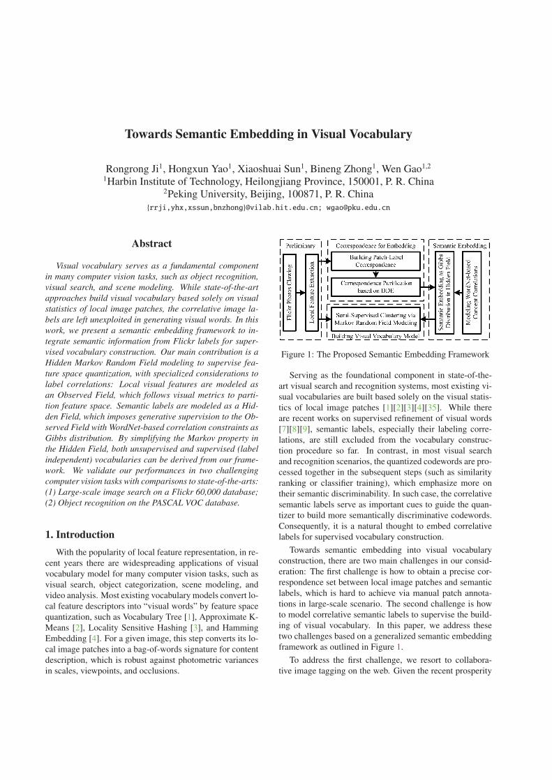
Figure 1: The Proposed Semantic Embedding Framework

Serving as the foundational component in state-of-the-art visual search and recognition systems, most existing vi-sual vocabularies are built based solely on the visual statis-tics of local image patches [1][2][3][4][35]. While thereare recent works on supervised refinement of visual words[7][8][9], semantic labels, especially their labeling corre-lations, are still excluded from the vocabulary construc-tion procedure so far. In contrast, in most visual searchand recognition scenarios, the quantized codewords are pro-cessed together in the subsequent steps (such as similarityranking or classifier training), which emphasize more ontheir semantic discriminability. In such case, the correlativesemantic labels serve as important cues to guide the quan-tizer to build more semantically discriminative codewords.Consequently, it is a natural thought to embed correlativelabels for supervised vocabulary construction.

Towards semantic embedding into visual vocabularyconstruction, there are two main challenges in our consid-eration: The first challenge is how to obtain a precise cor-respondence set between local image patches and semanticlabels, which is hard to achieve via manual patch annota-tions in large-scale scenario. The second challenge is howto model correlative semantic labels to supervise the build-ing of visual vocabulary. In this paper, we address thesetwo challenges based on a generalized semantic embeddingframework as outlined in Figure 1.

To address the first challenge, we resort to collabora-tive image tagging on the web. Given the recent prosperity

of image sharing websites such as Flickr, nowadays thereare millions of manually annotated photos available on theWeb. These data enable us to incorporate collaborativehuman knowledge to supervise the visual vocabulary con-struction in large-scale, real-world scenario. We present aDensity-Diversity Estimation (DDE) scheme in Section 2to build precise patch-label correspondences from openingavailable, user-labeled Flickr photo collections.

To address the second challenge, given a set of local fea-tures with (partial) semantic labels, we introduce a HiddenMarkov Random Field to model the supervision from cor-relative semantic labels to local image patches in Section 3.Our model consists of two layers (outlined in Figure 3): TheObserved Field layer contains local features extracted fromthe entire image database, where visual metric takes effectto quantize the feature space into codeword subregions. TheHidden Field layer models (partial) semantic labels withWordNet-based correlation constraints. Semantics in theHidden Field follow the Markov property to produce Gibbsdistribution over local features in the Observed Field, whichgives generative supervision to jointly optimize the localfeature quantization procedure.

Our further contributions are summarized as follows:1. We publish a ground truth set of patch-label corre-

spondences for semantic embedding [32]. In particular, thisdataset contains over 18 million local features with over450,000 user labels (over 3,600 unique keywords). It isthe first large-scale patch labeling set in literature for su-pervised vocabulary learning.

2. Our model is generalized for many existing vocab-ulary construction methods: By simplifying the Markovproperties in the Hidden Field, our model can be degener-ated into both supervised and unsupervised vocabulary con-structions, e.g. k means and vocabulary tree [1].

3. By introducing WordNet-based label correlations inGibbs distribution, our semantic embedding approach canhandle thousands of different labels with complicated cor-relations. This goes beyond previous approaches [7][8][9]that can only handle hundreds of labels at most.

Our work is inspired by the work from semi-supervisedclustering [6], where both must-link and cannot-link con-straints are provided to restrict the data clustering processwithin a Markov Random Field framework. In terms offunctionality, the closest works to ours derive from thelearning-based codebook constructions [7][8][9]. Mairalet al. [7] built a supervised vocabulary by learning dis-criminative and sparse coding models for object categoriza-tion. Lazebnik et al. [8] proposed to construct supervisedcodebooks by minimizing mutual information lost to in-dex fully labeled data. Moosmann et al. [9] proposed anERC-Forest to consider semantic labels as stopping tests inbuilding supervised indexing trees. Another group of re-lated works [13][14][15] refines (merges or splits) the initial

codewords to build class(image)-specific vocabularies forcategorization. Although working well for limited-numbercategories, these approaches cannot be scaled up to general-ized scenarios with numerous and semantically correlativecategories. Similar works can also be referred to the Learn-ing Vector Quantization [10][11][12] in data compression,which adopted self-organizing maps [11] or regression lostminimization [12] to build codebook that minimizes train-ing data distortions after compression. To a certain degree,similarities also exist between our work and topic decompo-sitions (pLSA [16] or LDA [17]). There are also previousworks in learning visual parts [19][20] by clustering localpatches with spatial configurations. By exploiting seman-tics learning in visual representation stage, our work dif-fers from works that adopt semantic learning to refine thesubsequent recognition stages [21][22][23], e.g. classifiersbased on machine translation [21] or semantic hierarchy[22]. The main issue for these approaches lies in ignoringconcept correlations in quantization, thus cannot actuallybuild supervised vocabulary with correlative labels. Fur-thermore, the current learning-based visual representations[7][8][9][13][14][15][16][17] obtained labels from the en-tire image, hence included background clutters to degener-ate learning effectiveness, which we addressed in Section 2.

In our quantitative validations (Section 4), we evaluateour performance on two challenging tasks: (1) The imagesearch task on a Flickr dataset containing 60,000 photos, inwhich we compare our retrieval MAP with the VocabularyTree model [1] and GNP [34]; (2) The object recognitiontask in PASCAL VOC, in which we compare our recogni-tion precision with two state-of-the-art supervised vocabu-lary building approaches [13][24].

2. Building Correspondences from Flickr

The input of our semantic embedding is a set of corre-spondences from local feature patches to semantic labels.Each correspondence offers a unique label and a set of localfeatures extracted from photos with this label. In the tra-ditional approaches, such patch-label correspondences arecollected by either manual annotations or from the entiretraining image. For the latter case, labeling noises are anunaddressed problem in the large-scale scenario. To han-dle this problem, we present a Density Diversity Estimation(DDE) approach to purify the patch-label correspondencescollected from Flickr photos with collaborative labels.

2.1. Collecting Correspondences from Flickr

We collected over 60,000 photos with labels from Flickr.For each photo, Difference of Gaussian salient regions aredetected and described by SIFT [30]. Each correspondencecontains a label and a set of SIFT patches extracted fromFlickr photos with this label. We discard infrequent label in

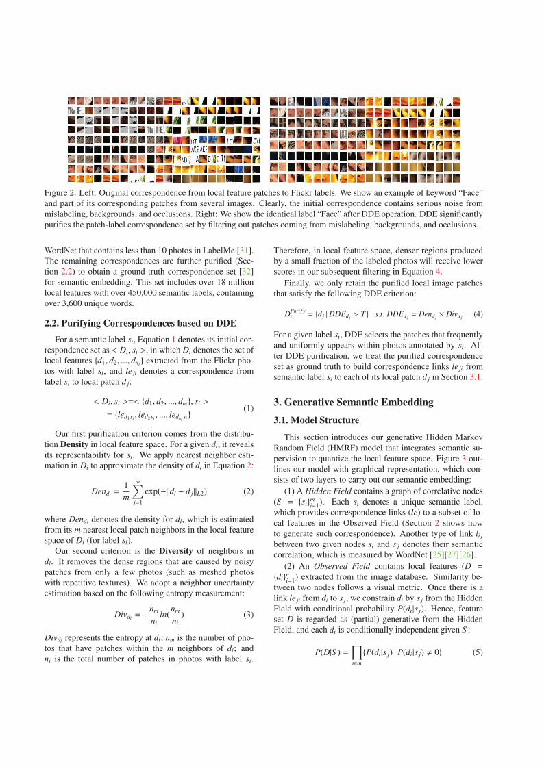
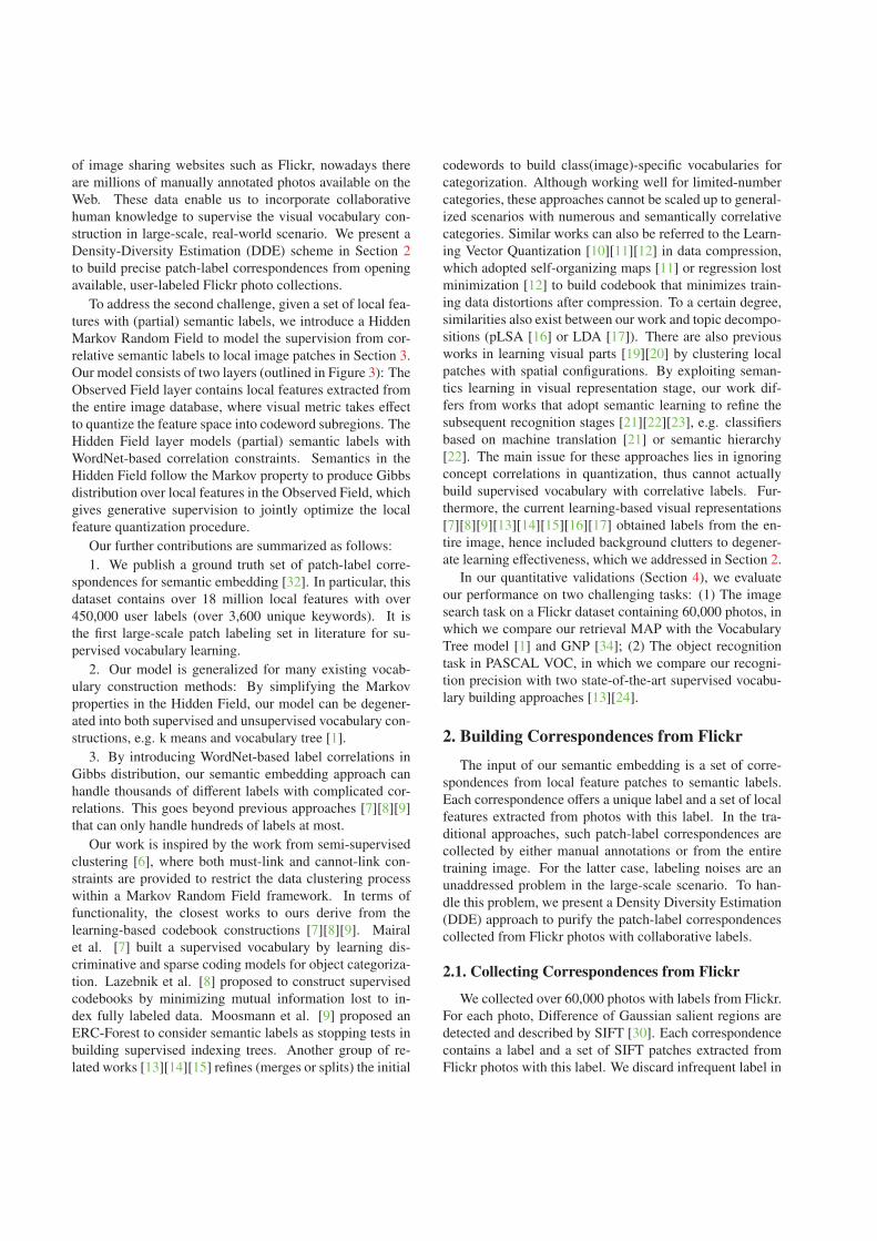
Figure 2: Left: Original correspondence from local feature patches to Flickr labels. We show an example of keyword “Face”and part of its corresponding patches from several images. Clearly, the initial correspondence contains serious noise frommislabeling, backgrounds, and occlusions. Right: We show the identical label “Face” after DDE operation. DDE significantlypurifies the patch-label correspondence set by filtering out patches coming from mislabeling, backgrounds, and occlusions.

WordNet that contains less than 10 photos in LabelMe [31].The remaining correspondences are further purified (Sec-tion 2.2) to obtain a ground truth correspondence set [32]for semantic embedding. This set includes over 18 millionlocal features with over 450,000 semantic labels, containingover 3,600 unique words.

2.2. Purifying Correspondences based on DDE

For a semantic label si, Equation 1 denotes its initial cor-respondence set as < Di, si >, in which Di denotes the set oflocal features {d1, d2, ..., dni } extracted from the Flickr pho-tos with label si, and le ji denotes a correspondence fromlabel si to local patch d j:

< Di, si >=< {d1, d2, ..., dni }, si >

= {led1 si , led2 si , ..., ledni si }(1)

Our first purification criterion comes from the distribu-tion Density in local feature space. For a given dl, it revealsits representability for si. We apply nearest neighbor esti-mation in Di to approximate the density of dl in Equation 2:

Dendl =1m

m∑

j=1

exp(−||dl − d j||L2) (2)

where Dendl denotes the density for dl, which is estimatedfrom its m nearest local patch neighbors in the local featurespace of Di (for label si).

Our second criterion is the Diversity of neighbors indl. It removes the dense regions that are caused by noisypatches from only a few photos (such as meshed photoswith repetitive textures). We adopt a neighbor uncertaintyestimation based on the following entropy measurement:

Divdl = −nm

niln(

nm

ni) (3)

Divdl represents the entropy at dl; nm is the number of pho-tos that have patches within the m neighbors of dl; andni is the total number of patches in photos with label si.

Therefore, in local feature space, denser regions producedby a small fraction of the labeled photos will receive lowerscores in our subsequent filtering in Equation 4.

Finally, we only retain the purified local image patchesthat satisfy the following DDE criterion:

DPuri f yi = {dj |DDEd j > T } s.t. DDEd j = Dend j × Divd j (4)

For a given label si, DDE selects the patches that frequentlyand uniformly appears within photos annotated by si. Af-ter DDE purification, we treat the purified correspondenceset as ground truth to build correspondence links le ji fromsemantic label si to each of its local patch d j in Section 3.1.

3. Generative Semantic Embedding

3.1. Model Structure

This section introduces our generative Hidden MarkovRandom Field (HMRF) model that integrates semantic su-pervision to quantize the local feature space. Figure 3 out-lines our model with graphical representation, which con-sists of two layers to carry out our semantic embedding:

(1) A Hidden Field contains a graph of correlative nodes(S = {si}mi=1). Each si denotes a unique semantic label,which provides correspondence links (le) to a subset of lo-cal features in the Observed Field (Section 2 shows howto generate such correspondence). Another type of link li j

between two given nodes si and s j denotes their semanticcorrelation, which is measured by WordNet [25][27][26].

(2) An Observed Field contains local features (D =

{di}ni=1) extracted from the image database. Similarity be-tween two nodes follows a visual metric. Once there is alink le ji from di to s j, we constrain di by s j from the HiddenField with conditional probability P(di|s j). Hence, featureset D is regarded as (partial) generative from the HiddenField, and each di is conditionally independent given S :

P(D|S ) =∏

i∈m{P(di|s j) | P(di|s j) � 0} (5)

Figure 3: Semantic Embedding by Markov Random Field

We assign a unique cluster label ci to each di. Therefore,D is quantized into a visual vocabularyW = {wk}Kk=1 (Cor-responding feature vectors V = {vk}Kk=1). The quantizer as-signment for D is denoted as C = {ci}ni=1. ci = c j = wk de-notes di and d j belong to an identical visual word wk. FromFigure 3, the vocabularyW and the semantics S are condi-tionally dependent given the Observed Field, which therebyincorporates S to optimize the building ofW.

3.2. Generative Embedding

We define a Markov Random Field on the Hidden Field,which imposes Markov probability distribution to supervisethe quantizer assignments C of D in the Observed Field:

∀i P(ci|C) = P(ci | {c j | le jx � 0, leiy � 0, x ∈ N′y}) (6)

Here, x and y are nodes in the Hidden Field that links topoints i and j in the Observed Field respectively (le jx andleiy � 0). N′y is the Hidden Field neighborhood of y. Thecluster label ci depends on its neighborhood cluster labels({c j}. This “neighborhood” definition is within the HiddenField. i.e. each c j is the cluster assignment of dj that haveneighborhood labels (sx) within N′y for sy of di.

Considering a particular configuration of quantizer as-signments C (which gives a “visual vocabulary” represen-tation), its probability can be expressed as a Gibbs distri-bution [28] generated from the Hidden Field, depending onthe following Hammersley-Clifford theorem [29]:

P(C) =1H exp (−L(C)) =

1H exp (−

K∑

k=1

LNk (wk)) (7)

H is a normalization constraint, and L(C) is the overallpotential function for the current quantizer assignment C,which can be decomposed into the sum of potential func-tions LNk (wk) for each visual word wk, which only consid-ers influences from points in wk (volume Nk).

Two data points di and d j in wk contribute to LNk (wk)if and only if: (1) correspondence links lexi and ley j existfrom di and d j to semantic nodes sx and sy respectively;and (2) semantic correlation lxy exists between sx and sy inthe Hidden Field. We resort to WordNet::Similarity [27] tomeasure lxy, which is constrained to [0, 1] with lxx = 1. Alarge lxy means a close semantic correlation (usually from

correlative nouns e.g. “rose” and “flower”). In Equation 8,We minus the sum of lxy to fit the potential function L(C).Intuitively, P(C) gives higher probabilities to quantizer thatfollows semantic constraints better. We calculate P(C) by:

P(C) =1H exp (−

K∑

k=1

LNk (wk))

=1H exp (−

K∑

k=1

∑

i∈Nk

∑

j∈Nk

{−lxy | lexi � 0 ∧ ley j � 0

})

(8)

3.3. Iterative Quantization

We consider D = {di}ni=1 in the Observed Field as gener-ative from a particular quantizer configuration C = {ci}ni=1through its conditional probability distribution P(D|C):

P(D|C) =n∑

i=1

P(di|ci) =n∑

i=1

{P(di, vk) | ci = wk} (9)

Given ci, the probability density P(di, vk) is measured by thevisual similarity between feature point di and its visual wordfeature vk. To obtain the best C, we investigate the overallposterior probability of a given C as P(C|D) = P(D|C)P(C),in which we consider the probability of P(D) as a constraint.Finding Maximum-A-Posterior of P(C|D) can be convertedinto maximizing its posterior probability:

P(C|D) ∝ P(D|C)P(C) ∝⎛⎜⎜⎜⎜⎜⎝

n∑

i=1

{P(di, vk) | ci = wk}⎞⎟⎟⎟⎟⎟⎠×

⎛⎜⎜⎜⎜⎜⎜⎝1H exp (

K∑

k=1

∑

i∈Nk

∑

j∈Nk

{lxy | lexi � 0 ∧ ley j � 0})⎞⎟⎟⎟⎟⎟⎟⎠

(10)

Therefore, there are two criteria to optimize the quantiza-tion configuration C (and hence the vocabulary configura-tionW): (1) The visual constraint P(D|C) imposed by eachpoint di to its corresponding word feature vk, which is re-garded as the quantization distortions of all visual words:

n∑

i=1

{P(di, vk) | ci = wk}

∝ exp (−n∑

i=1

{Dis(di, vk) | ci = wk})(11)

(2) The semantic constraints P(C) imposed from the HiddenField, which are measured as:

1H exp (

K∑

k=1

∑

i∈Nk

∑

j∈Nk

{lxy | lexi � 0 ∧ ley j � 0}) (12)

Due to the constraints in P(C), MAP cannot be solved as amaximum likelihood. Furthermore, since the quantizer as-signment C and the centroid feature vectors V could not

be obtained simultaneously, we cannot directly optimizethe quantization in Equation 10. We address this by a K-Means clustering, which works in an Estimation Maximiza-tion manner to estimate the probability cluster membership:

The E Step updates the quantizer assignment C us-ing the MAP estimation at the current iteration. Dif-ferent from the traditional K-Means clustering, we inte-grate the correlations between data points by imposing1H exp (

∑Kk=1∑

i∈Nk

∑j∈Nk{lxy | lexi � 0 ∧ ley j � 0}) to select-

ing configuration C. The quantizer assignment for each di

is performed in a random order, which assigns wk to di thatminimizes the contribution of di to the objective function.Therefore, Ob j(C|D) �

∑ni=1 Ob j(ci|di). Without losing

generality, we give a log estimation from Equation 10 todefine the Ob j(ci|di) for each di as follows:

Ob j(ci|di) = arg mink(−Dis(di, vk)+1H′∑

j∈Nk

{lxy | lexi � 0 ∧ ley j � 0}) (13)

The M Step re-estimates the K cluster centroid vectors{vk}Kk=1 from visual data assigned to them in the current EStep, which minimizes Ob j(ci|di) in Equation 13 (equiva-lent to maximize the expects of “visual words”). We updatethe kth centroid vector vk based on the visual data within wk:

vk =

∑di∈Wk

di

||Wk || s.t. Wk = {di|ci = wk} (14)

3.4. Model Generalization

Ignoring links between nodes in the Hidden Field wouldlead to supervised quantization with isolated and indepen-dent supervision, which is the similar settlements of [7][8][9][10][11][12]. Based on this independency settlement,our model only needs to modify P(C) from Equation 7 to:

P(C) =1H exp (−

∑

Ni∈NLNi (wi))

=1H exp (−

K∑

k=1

∑

i∈Nk

∑

j∈Nk

{−�lxy� | lexi � 0 ∧ ley j � 0})(15)

Uncorrelated supervision are hence ensured (�lxy� = 0 ifx � y). And Equation 13 is then rewritten into:

Ob j(ci|di) = arg mink(−Dis(di, vk)

+1H′∑

j∈Nk

{�lxy� | lexi � 0 ∧ ley j � 0}) (16)

Since only identical words (i = j) will produce lxy = 1,semantic correlations are ignored in Equations 15 and 16.If we further set �lxy� in Equation 15 as 0, supervision fromHidden Field will be totally removed, which then simplifiesour model into an unsupervised clustering.

Algorithm 1: Building Supervised Visual Vocabulary1 Input: Visual data D = {di}ni=1, Semantic supervision

S = {s j}mj=1, Correspondence set {LE1, ..., LEm}, andSemantic correlation li j for any two si and s j calculated byWordNet::Similarity[27], Maximum iteration NI .

2 Pre-computing: Calculate the nearest neighbors in theHidden Field using an o(m2) sequential scanning heap.Initialize a random set of clustering centersW = {wk}Kk=1.

3 Iterative EM Steps:while {V = {vk}Kk=1 still changse or thenumber of iteration is within NI} do

4 E Step: For each di in D, assign ci = wk that satisfyingthe objective function in Equation 13, in which nearestneighbors in the Hidden Field are obtained frompre-computing (Step 2).

5 M Step: For each wk inW, update its correspondingfeature vector vk based on Equation 14.

6 end7 Output: Supervised vocabulary C = {ck}Kk=1 with its inverted

indexing structure (Indexed after EM).

3.5. Vocabulary Building Flow

Finally, we present our implementation details in build-ing both single-level and hierarchical visual vocabulariesbased on our semantic embedding model as follows:

Single-Level Vocabulary: Algorithm 1 presents thebuilding flow of single-level vocabulary. Our time cost isalmost identical to the traditional K-Means clustering. Theonly additional cost is the nearest neighbor calculation inthe Hidden Field for P(C), which can be performed usingan o(m2) sequential scanning for m semantic labels (eachwith a heap ranking) and stored beforehand.

Hierarchical Vocabulary: Many large-scale retrievalapplications usually involve tens of thousands of images.To ensure online search efficiency, hierarchical quantizationis usually adopted, e.g. Vocabulary Tree (VT) [1], Approx-imate K-Means (AKM) [2], and their variations. We alsodeploy our semantic embedding to a hierarchical version,in which the Vocabulary Tree model [1] is adopted to builda visual vocabulary based on hierarchical K-Means cluster-ing. Comparing with single-level quantization, the Vocab-ulary Tree (VT) model pays extreme focus to the searchefficiency: To produce a bag-of-words vector for an im-age using a w-branch m-word VT model, the time cost isO(w log(w(m))), whereas using a single-level word division,the time cost is O(m). During hierarchical clustering, oursemantic embedding is identical within each subcluster.

4. Experimental ComparisonsWe give two groups of quantitative comparisons in our

experiments. The first group shows the advantages of ourGenerative Semantic Embedding (GSE) to the unsupervisedvocabulary construction schemes, including comparisons to

(1) traditional Vocabulary Tree (VT) [1] and GNP [34], and(2) GSE without semantic correlations (ignoring semanticlinks in the Hidden Field graph to infer P(C)). The sec-ond group compares our GSE model with two related worksin building supervised vocabulary for object recognitiontasks: (1) Class-specific adaptive vocabulary [13], and (2)Learning-based visual word merging [24]. During compar-ison, we also investigate how the Vocabulary Sparsity, Em-bedding Strength, and Label Noise (for which these mean-ing would be explained later) affect our performance.

4.1. Databases, Implementations, and Evaluations

Evaluation Databases: Two databases are adopted inevaluation: (1) The Flickr database contains over 60,000collaboratively labeled photos, which gives a real-worldevaluation for our first group OF experiments. It includesover 18 million local features with over 450,000 user labels(over 3,600 unique keywords). For Flickr, we randomly se-lect 2,000 photos to form a query set, and use the remaining58,000 to build our search model. (2) The PASCAL VOC05 database [33] evaluates our second group of experiments.We adopt VOC 05 instead of 08 since the former directlygives quantitative comparisons to [24], which is most re-lated to our work. We split PASCAL into two equal-sizedsets for training and testing, which is identical to the settle-ment in [24]. The PASCAL training set provides boundingboxes for image regions with annotations, which naturallygives us the purified patch-label correspondences.

Model Implementations: In the Flickr database, webuild a 10-branch, 4-level Vocabulary Tree for semantic em-bedding, based on the SIFT features extracted from the en-tire database. If a node has fewer than 2,000 features, westop its K-Means division, whether it has achieved the deep-est level or not. A document list (approximately 10,000words) is built for each word to record which photo con-tains this word, thus forms an inverted index file. In theonline part, each SIFT feature extracted from the query im-age is sent to its nearest visual word, in which the indexedimages are picked out to rank the similarity scores to thequery. As a baseline approach, we build a 10-branch, 4-level unsupervised Vocabulary Tree for the Flickr database.The same implementations are carried out for the PASCALdatabase, in which we reduce the number of hierarchicallayers to 3 to produce a visual vocabulary with visual wordvolume ≈ 1, 000.

Evaluation Criterion: We use Mean Average Precision(MAP) to evaluate our performances on Flickr. MAP inves-tigates whether a retrieval system can return more relevantdocuments earlier. It also reveals search precision with re-call (by dividing “#relevant image o f Query q”) and is sen-sitive to the ranking positions. (rq is the rank, N is the num-ber of retrieved images for q, and relq is a binary functionon the relevance of a given rank, Pq is precision at a given

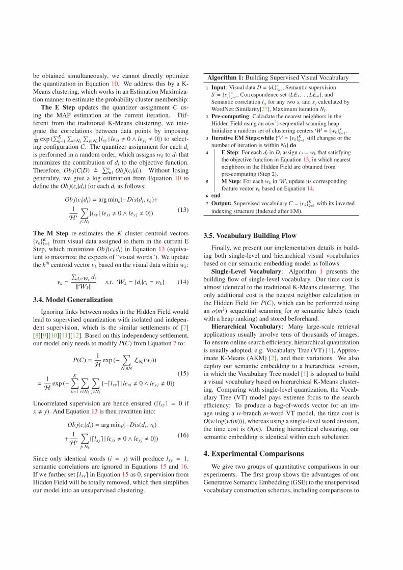
Figure 4: Case study of ratios between inter-class distanceand intra-class distance with and without semantic embed-ding in the Flickr dataset.

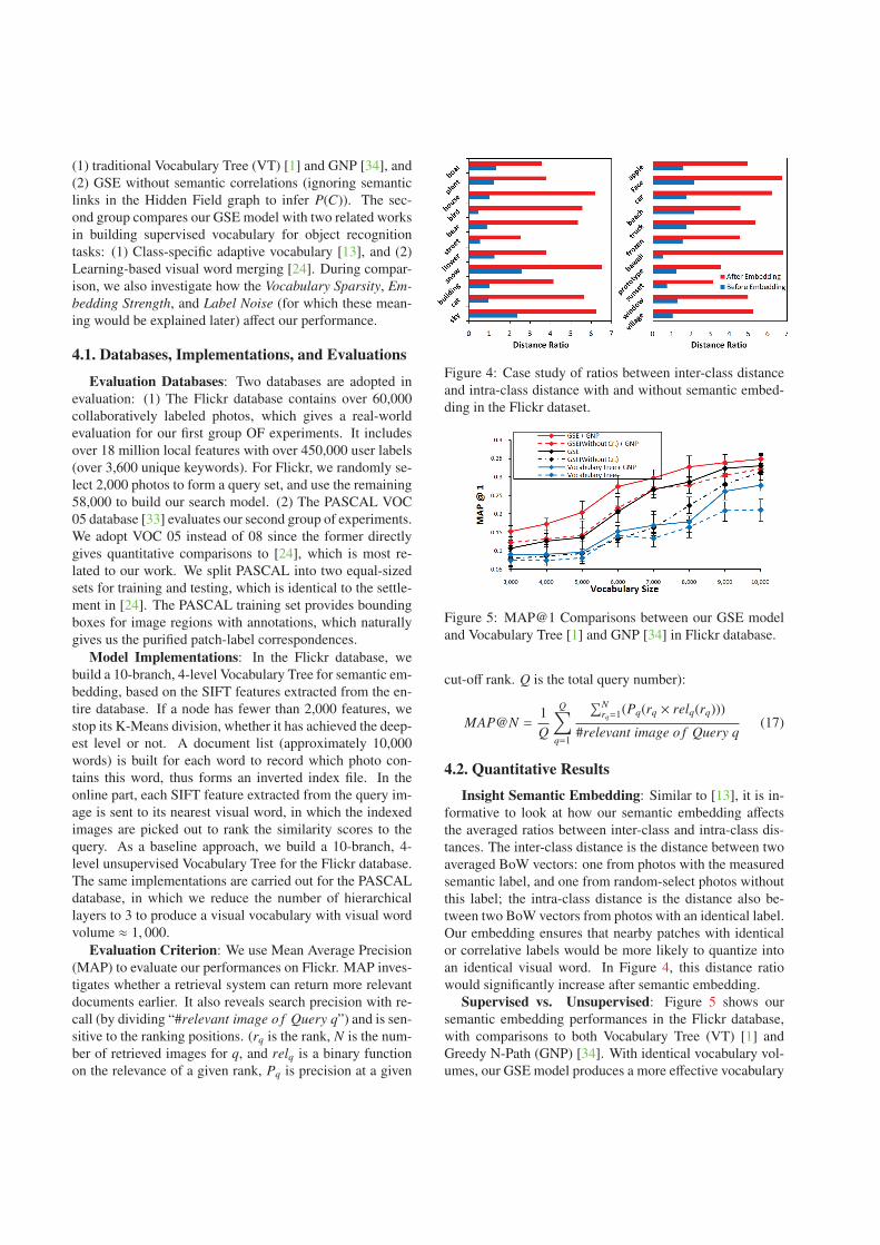
Figure 5: MAP@1 Comparisons between our GSE modeland Vocabulary Tree [1] and GNP [34] in Flickr database.

cut-off rank. Q is the total query number):

MAP@N =1Q

Q∑

q=1

∑Nrq=1(Pq(rq × relq(rq)))

#relevant image o f Query q(17)

4.2. Quantitative Results

Insight Semantic Embedding: Similar to [13], it is in-formative to look at how our semantic embedding affectsthe averaged ratios between inter-class and intra-class dis-tances. The inter-class distance is the distance between twoaveraged BoW vectors: one from photos with the measuredsemantic label, and one from random-select photos withoutthis label; the intra-class distance is the distance also be-tween two BoW vectors from photos with an identical label.Our embedding ensures that nearby patches with identicalor correlative labels would be more likely to quantize intoan identical visual word. In Figure 4, this distance ratiowould significantly increase after semantic embedding.

Supervised vs. Unsupervised: Figure 5 shows oursemantic embedding performances in the Flickr database,with comparisons to both Vocabulary Tree (VT) [1] andGreedy N-Path (GNP) [34]. With identical vocabulary vol-umes, our GSE model produces a more effective vocabulary

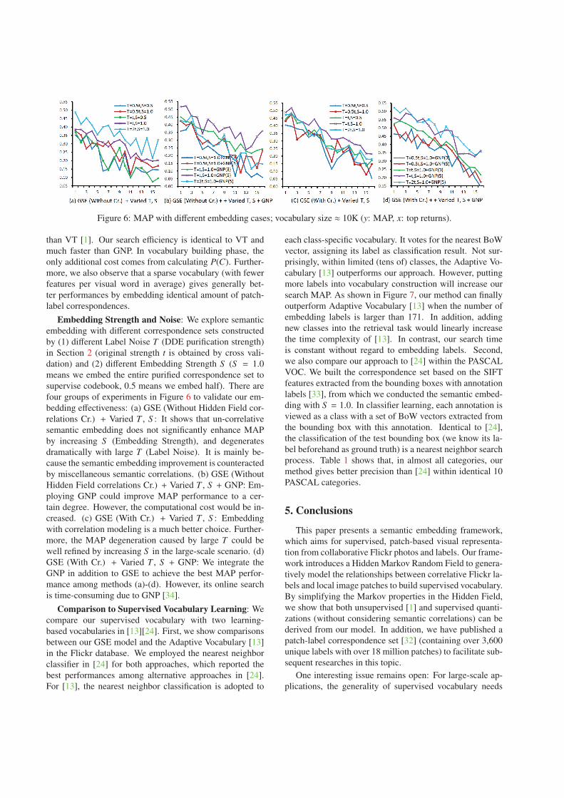
Figure 6: MAP with different embedding cases; vocabulary size ≈ 10K (y: MAP, x: top returns).

than VT [1]. Our search efficiency is identical to VT andmuch faster than GNP. In vocabulary building phase, theonly additional cost comes from calculating P(C). Further-more, we also observe that a sparse vocabulary (with fewerfeatures per visual word in average) gives generally bet-ter performances by embedding identical amount of patch-label correspondences.

Embedding Strength and Noise: We explore semanticembedding with different correspondence sets constructedby (1) different Label Noise T (DDE purification strength)in Section 2 (original strength t is obtained by cross vali-dation) and (2) different Embedding Strength S (S = 1.0means we embed the entire purified correspondence set tosupervise codebook, 0.5 means we embed half). There arefour groups of experiments in Figure 6 to validate our em-bedding effectiveness: (a) GSE (Without Hidden Field cor-relations Cr.) + Varied T , S : It shows that un-correlativesemantic embedding does not significantly enhance MAPby increasing S (Embedding Strength), and degeneratesdramatically with large T (Label Noise). It is mainly be-cause the semantic embedding improvement is counteractedby miscellaneous semantic correlations. (b) GSE (WithoutHidden Field correlations Cr.) + Varied T , S + GNP: Em-ploying GNP could improve MAP performance to a cer-tain degree. However, the computational cost would be in-creased. (c) GSE (With Cr.) + Varied T , S : Embeddingwith correlation modeling is a much better choice. Further-more, the MAP degeneration caused by large T could bewell refined by increasing S in the large-scale scenario. (d)GSE (With Cr.) + Varied T , S + GNP: We integrate theGNP in addition to GSE to achieve the best MAP perfor-mance among methods (a)-(d). However, its online searchis time-consuming due to GNP [34].

Comparison to Supervised Vocabulary Learning: Wecompare our supervised vocabulary with two learning-based vocabularies in [13][24]. First, we show comparisonsbetween our GSE model and the Adaptive Vocabulary [13]in the Flickr database. We employed the nearest neighborclassifier in [24] for both approaches, which reported thebest performances among alternative approaches in [24].For [13], the nearest neighbor classification is adopted to

each class-specific vocabulary. It votes for the nearest BoWvector, assigning its label as classification result. Not sur-prisingly, within limited (tens of) classes, the Adaptive Vo-cabulary [13] outperforms our approach. However, puttingmore labels into vocabulary construction will increase oursearch MAP. As shown in Figure 7, our method can finallyoutperform Adaptive Vocabulary [13] when the number ofembedding labels is larger than 171. In addition, addingnew classes into the retrieval task would linearly increasethe time complexity of [13]. In contrast, our search timeis constant without regard to embedding labels. Second,we also compare our approach to [24] within the PASCALVOC. We built the correspondence set based on the SIFTfeatures extracted from the bounding boxes with annotationlabels [33], from which we conducted the semantic embed-ding with S = 1.0. In classifier learning, each annotation isviewed as a class with a set of BoW vectors extracted fromthe bounding box with this annotation. Identical to [24],the classification of the test bounding box (we know its la-bel beforehand as ground truth) is a nearest neighbor searchprocess. Table 1 shows that, in almost all categories, ourmethod gives better precision than [24] within identical 10PASCAL categories.

5. Conclusions

This paper presents a semantic embedding framework,which aims for supervised, patch-based visual representa-tion from collaborative Flickr photos and labels. Our frame-work introduces a Hidden Markov Random Field to genera-tively model the relationships between correlative Flickr la-bels and local image patches to build supervised vocabulary.By simplifying the Markov properties in the Hidden Field,we show that both unsupervised [1] and supervised quanti-zations (without considering semantic correlations) can bederived from our model. In addition, we have published apatch-label correspondence set [32] (containing over 3,600unique labels with over 18 million patches) to facilitate sub-sequent researches in this topic.

One interesting issue remains open: For large-scale ap-plications, the generality of supervised vocabulary needs

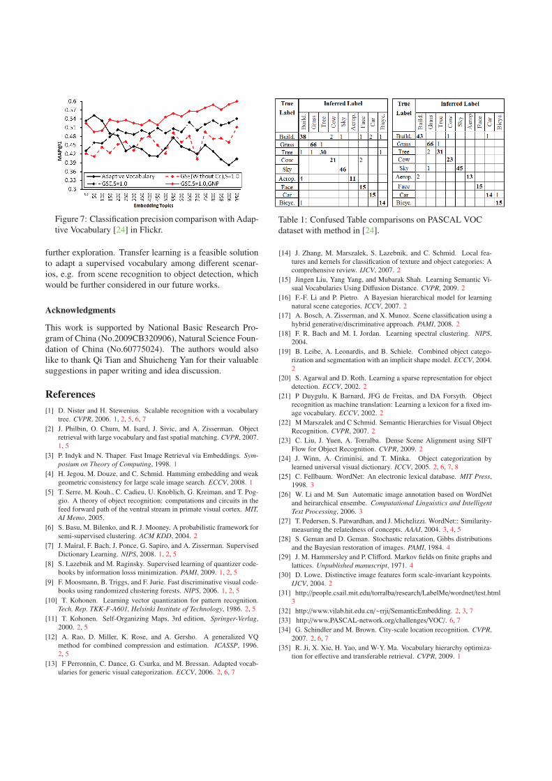
Figure 7: Classification precision comparison with Adap-tive Vocabulary [24] in Flickr.

Table 1: Confused Table comparisons on PASCAL VOCdataset with method in [24].

further exploration. Transfer learning is a feasible solutionto adapt a supervised vocabulary among different scenar-ios, e.g. from scene recognition to object detection, whichwould be further considered in our future works.

Acknowledgments

This work is supported by National Basic Research Pro-gram of China (No.2009CB320906), Natural Science Foun-dation of China (No.60775024). The authors would alsolike to thank Qi Tian and Shuicheng Yan for their valuablesuggestions in paper writing and idea discussion.

References[1] D. Nister and H. Stewenius. Scalable recognition with a vocabulary

tree. CVPR, 2006. 1, 2, 5, 6, 7[2] J. Philbin, O. Chum, M. Isard, J. Sivic, and A. Zisserman. Object

retrieval with large vocabulary and fast spatial matching. CVPR, 2007.1, 5

[3] P. Indyk and N. Thaper. Fast Image Retrieval via Embeddings. Sym-posium on Theory of Computing, 1998. 1

[4] H. Jegou, M. Douze, and C. Schmid. Hamming embedding and weakgeometric consistency for large scale image search. ECCV, 2008. 1

[5] T. Serre, M. Kouh., C. Cadieu, U. Knoblich, G. Kreiman, and T. Pog-gio. A theory of object recognition: computations and circuits in thefeed forward path of the ventral stream in primate visual cortex. MIT,AI Memo, 2005.

[6] S. Basu, M. Bilenko, and R. J. Mooney. A probabilistic framework forsemi-supervised clustering. ACM KDD, 2004. 2

[7] J. Mairal, F. Bach, J. Ponce, G. Sapiro, and A. Zisserman. SupervisedDictionary Learning. NIPS, 2008. 1, 2, 5

[8] S. Lazebnik and M. Raginsky. Supervised learning of quantizer code-books by information losss minimization. PAMI, 2009. 1, 2, 5

[9] F. Moosmann, B. Triggs, and F. Jurie. Fast discriminative visual code-books using randomized clustering forests. NIPS, 2006. 1, 2, 5

[10] T. Kohonen. Learning vector quantization for pattern recognition.Tech. Rep. TKK-F-A601, Helsinki Institute of Technology, 1986. 2, 5

[11] T. Kohonen. Self-Organizing Maps, 3rd edition, Springer-Verlag,2000. 2, 5

[12] A. Rao, D. Miller, K. Rose, and A. Gersho. A generalized VQmethod for combined compression and estimation. ICASSP, 1996.2, 5

[13] F Perronnin, C. Dance, G. Csurka, and M. Bressan. Adapted vocab-ularies for generic visual categorization. ECCV, 2006. 2, 6, 7

[14] J. Zhang, M. Marszalek, S. Lazebnik, and C. Schmid. Local fea-tures and kernels for classification of texture and object categories: Acomprehensive review. IJCV, 2007. 2

[15] Jingen Liu, Yang Yang, and Mubarak Shah. Learning Semantic Vi-sual Vocabularies Using Diffusion Distance. CVPR, 2009. 2

[16] F.-F. Li and P. Pietro. A Bayesian hierarchical model for learningnatural scene categories. ICCV, 2007. 2

[17] A. Bosch, A. Zisserman, and X. Munoz. Scene classification using ahybrid generative/discriminative approach. PAMI, 2008. 2

[18] F. R. Bach and M. I. Jordan. Learning spectral clustering. NIPS,2004.

[19] B. Leibe, A. Leonardis, and B. Schiele. Combined object catego-rization and segmentation with an implicit shape model. ECCV, 2004.2

[20] S. Agarwal and D. Roth. Learning a sparse representation for objectdetection. ECCV, 2002. 2

[21] P Duygulu, K Barnard, JFG de Freitas, and DA Forsyth. Objectrecognition as machine translation: Learning a lexicon for a fixed im-age vocabulary. ECCV, 2002. 2

[22] M Marszalek and C Schmid. Semantic Hierarchies for Visual ObjectRecognition. CVPR, 2007. 2

[23] C. Liu, J. Yuen, A. Torralba. Dense Scene Alignment using SIFTFlow for Object Recognition. CVPR, 2009. 2

[24] J. Winn, A. Criminisi, and T. Minka. Object categorization bylearned universal visual dictionary. ICCV, 2005. 2, 6, 7, 8

[25] C. Fellbaum. WordNet: An electronic lexical database. MIT Press,1998. 3

[26] W. Li and M. Sun Automatic image annotation based on WordNetand heirarchical ensembe. Computational Linguistics and IntelligentText Processing, 2006. 3

[27] T. Pedersen, S. Patwardhan, and J. Michelizzi. WordNet:: Similarity-measuring the relatedness of concepts. AAAI, 2004. 3, 4, 5

[28] S. Geman and D. Geman. Stochastic relaxation, Gibbs distributionsand the Bayesian restoration of images. PAMI, 1984. 4

[29] J. M. Hammersley and P. Clifford. Markov fields on finite graphs andlattices. Unpublished manuscript, 1971. 4

[30] D. Lowe. Distinctive image features form scale-invariant keypoints.IJCV, 2004. 2

[31] http://people.csail.mit.edu/torralba/research/LabelMe/wordnet/test.html3

[32] http://www.vilab.hit.edu.cn/∼rrji/SemanticEmbedding. 2, 3, 7[33] http://www.PASCAL-network.org/challenges/VOC/. 6, 7[34] G. Schindler and M. Brown. City-scale location recognition. CVPR,

2007. 2, 6, 7[35] R. Ji, X. Xie, H. Yao, and W-Y. Ma. Vocabulary hierarchy optimiza-

tion for effective and transferable retrieval. CVPR, 2009. 1