TOWARDS SCORE FOLLOWING IN SHEET MUSIC IMAGES

Matthias Dorfer Andreas Arzt Gerhard WidmerDepartment of Computational Perception, Johannes Kepler University Linz, Austria

matthias.dorfer@jku.at

ABSTRACT

This paper addresses the matching of short music audiosnippets to the corresponding pixel location in images ofsheet music. A system is presented that simultaneouslylearns to read notes, listens to music and matches thecurrently played music to its corresponding notes in thesheet. It consists of an end-to-end multi-modal convolu-tional neural network that takes as input images of sheetmusic and spectrograms of the respective audio snippets.It learns to predict, for a given unseen audio snippet (cov-ering approximately one bar of music), the correspondingposition in the respective score line. Our results suggestthat with the use of (deep) neural networks – which haveproven to be powerful image processing models – workingwith sheet music becomes feasible and a promising futureresearch direction.

1. INTRODUCTION

Precisely linking a performance to its respective sheet mu-sic – commonly referred to as audio-to-score alignment –is an important topic in MIR and the basis for many appli-cations [20]. For instance, the combination of score andaudio supports algorithms and tools that help musicolo-gists in in-depth performance analysis (see e.g. [6]), al-lows for new ways to browse and listen to classical music(e.g. [9, 13]), and can generally be helpful in the creationof training data for tasks like beat tracking or chord recog-nition. When done on-line, the alignment task is known asscore following, and enables a range of applications likethe synchronization of visualisations to the live music dur-ing concerts (e.g. [1, 17]), and automatic accompanimentand interaction live on stage (e.g. [5, 18]).

So far all approaches to this task depend on a symbolic,computer-readable representation of the sheet music, suchas MusicXML or MIDI (see e.g. [1, 5, 8, 12, 14–18]). Thisrepresentation is created either manually (e.g. via the time-consuming process of (re-)setting the score in a music no-tation program), or automatically via optical music recog-nition software. Unfortunately automatic methods are stillhighly unreliable and thus of limited use, especially formore complex music like orchestral scores [20].

c© Matthias Dorfer, Andreas Arzt, Gerhard Widmer. Li-censed under a Creative Commons Attribution 4.0 International License(CC BY 4.0). Attribution: Matthias Dorfer, Andreas Arzt, GerhardWidmer. “Towards Score Following in Sheet Music Images”, 17th Inter-national Society for Music Information Retrieval Conference, 2016.

The central idea of this paper is to develop a method thatlinks the audio and the image of the sheet music directly,by learning correspondences between these two modali-ties, and thus making the complicated step of creating anin-between representation obsolete. We aim for an algo-rithm that simultaneously learns to read notes, listens tomusic and matches the currently played music with the cor-rect notes in the sheet music. We will tackle the problem inan end-to-end neural network fashion, meaning that the en-tire behaviour of the algorithm is learned purely from dataand no further manual feature engineering is required.

2. METHODS

This section describes the audio-to-sheet matching modeland the input data required, and shows how the model isused at test time to predict the expected location of a newunseen audio snippets in the respective sheet image.

2.1 Data, Notation and Task Description

The model takes two different input modalities at the sametime: images of scores, and short excerpts from spectro-grams of audio renditions of the score (we will call thesequery snippets as the task is to predict the position in thescore that corresponds to such an audio snippet). For thisfirst proof-of-concept paper, we make a number of simpli-fying assumptions: for the time being, the system is fedonly a single staff line at a time (not a full page of score).We restrict ourselves to monophonic music, and to the pi-ano. To generate training examples, we produce a fixed-length query snippet for each note (onset) in the audio.The snippet covers the target note onset plus a few addi-tional frames, at the end of the snippet, and a fixed-sizecontext of 1.2 seconds into the past, to give some temporalcontext. The same procedure is followed when producingexample queries for off-line testing.

A training/testing example is thus composed of two in-puts: Input 1 is an image Si (in our case of size 40 × 390pixels) showing one staff of sheet music. Input 2 is an au-dio snippet – specifically, a spectrogram excerpt Ei,j (40frames× 136 frequency bins) – cut from a recording of thepiece, of fixed length (1.2 seconds). The rightmost onsetin spectrogram excerpt Ei,j is interpreted as the target notej whose position we want to predict in staff image Si. Forthe music used in our experiments (Section 3) this contextis a bit less than one bar. For each note j (represented byits corresponding spectrogram excerpt Ei,j) we annotatedits ground truth sheet location xj in sheet image Si. Coor-

789

(a) Spectrogram-to-sheet correspondence. In this ex-ample the rightmost onset in spectrogram excerpt Ei,j

corresponds to the rightmost note (target note j) insheet image Si. For the present case the temporal con-text of about 1.2 seconds (into the past) covers fiveadditional notes in the spectrogram. The staff imageand spectrogram excerpt are exactly the multi-modalinput presented to the proposed audio-to-sheet match-ing network. At train time the target pixel location xj

in the sheet image is available; at test time xj has tobe predicted by the model (see figure below).

(b) Schematic sketch of the audio-to-sheet matching task targetedin this work. Given a sheet image Si and a short snippet of au-dio (spectrogram excerpt Ei,j ) the model has to predict the audiosnippet’s corresponding pixel location xj in the image.

Figure 1: Input data and audio-to-sheet matching task.

dinate xj is the distance of the note head (in pixels) fromthe left border of the image. As we work with single staffsof sheet music we only need the x-coordinate of the noteat this point. Figure 1a relates all components involved.

Summary and Task Description: For training we presenttriples of (1) staff image Si, (2) spectrogram excerpt Ei,j

and (3) ground truth pixel x-coordinate xj to our audio-to-sheet matching model. At test time only the staff imageand spectrogram excerpt are available and the task of themodel is to predict the estimated pixel location xj in theimage. Figure 1b shows a sketch summarizing this task.

2.2 Audio-Sheet Matching as Bucket Classification

We now propose a multi-modal convolutional neural net-work architecture that learns to match unseen audio snip-pets (spectrogram excerpts) to their corresponding pixel lo-cation in the sheet image.

2.2.1 Network Structure

Figure 2 provides a general overview of the deep networkand the proposed solution to the matching problem. Asmentioned above, the model operates jointly on a staff im-age Si and the audio (spectrogram) excerpt Ei,j related toa note j. The rightmost onset in the spectrogram excerptis the one related to target note j. The multi-modal model

consists of two specialized convolutional networks: onedealing with the sheet image and one dealing with the au-dio (spectrogram) input. In the subsequent layers we fusethe specialized sub-networks by concatenation of the latentimage- and audio representations and additional process-ing by a sequence of dense layers. For a detailed descrip-tion of the individual layers we refer to Table 1 in Section3.4. The output layer of the network and the correspondinglocalization principle are explained in the following.

2.2.2 Audio-to-Sheet Bucket Classification

The objective for an unseen spectrogram excerpt and a cor-responding staff of sheet music is to predict the excerpt’slocation xj in the staff image. For this purpose we startwith horizontally quantizing the sheet image into B non-overlapping buckets. This discretisation step is indicatedas the short vertical lines in the staff image above the scorein Figure 2. In a second step we create for each note j inthe train set a target vector tj = {tj,b} where each vec-tor element tj,b holds the probability that bucket b coversthe current target note j. In particular, we use soft tar-gets, meaning that the probability for one note is sharedbetween the two buckets closest to the note’s true pixel lo-cation xj . We linearly interpolate the shared probabilitiesbased on the two pixel distances (normalized to sum upto one) of the note’s location xj to the respective (closest)bucket centers. Bucket centers are denoted by cb in thefollowing where subscript b is the index of the respectivebucket. Figure 3 shows an example sketch of the compo-nents described above. Based on the soft target vectors wedesign the output layer of our audio-to-sheet matching net-work as a B-way soft-max with activations defined as:

φ(yj,b) =eyj,b

∑Bk=1 e

yj,k

(1)

φ(yj,b) is the soft-max activation of the output neuron rep-resenting bucket b and hence also representing the regionin the sheet image covered by this bucket. By applying thesoft-max activation the network output gets normalized torange (0, 1) and further sums up to 1.0 over all B outputneurons. The network output can now also be interpretedas a vector of probabilities pj = {φ(yj,b)} and shares thesame value range and properties as the soft target vectors.

In training, we optimize the network parameters Θ byminimizing the Categorical Cross Entropy (CCE) loss ljbetween target vectors tj and network output pj :

lj(Θ) = −B∑

k=1

tj,k log(pj,k) (2)

The CCE loss function becomes minimal when the net-work output pj exactly matches the respective soft targetvector tj . In Section 3.4 we provide further informationon the exact optimization strategy used. 1

1 For the sake of completeness: In our initial experiments we startedto predict the sheet location of audio snippets by minimizing the Mean-Squared-Error (MSE) between the predicted and the true pixel coordinate(MSE regression). However, we observed that training these networksis much harder and further performs worse than the bucket classificationapproach proposed in this paper.

790 Proceedings of the 17th ISMIR Conference, New York City, USA, August 7-11, 2016

Figure 2: Overview of multi-modal convolutional neural network for audio-to-sheet matching. The network takes a staff image anda spectrogram excerpt as input. Two specialized convolutional network parts, one for the sheet image and one for the audio input, aremerged into one multi-modality network. The output part of the network predicts the region in the sheet image – the classification bucket– to which the audio snippet corresponds.

Figure 3: Part of a staff of sheet music along with soft tar-get vector tj for target note j surrounded with an ellipse. Thetwo buckets closest to the note share the probability (indicated asdots) of containing the note. The short vertical lines highlight thebucket borders.

2.3 Sheet Location Prediction

Once the model is trained, we use it at test time to predictthe expected location xj of an audio snippet with targetnote j in a corresponding image of sheet music. The outputof the network is a vector pj = {pj,b} holding the prob-abilities that the given test snippet j matches with bucketb in the sheet image. Having these probabilities we con-sider two different types of predictions: (1) We computethe center c∗b of bucket b∗ = argmaxb pj,b holding the high-est overall matching probability. (2) For the second casewe take, in addition to b∗, the two neighbouring bucketsb∗ − 1 and b∗ + 1 into account and compute a (linearly)probability weighted position prediction in the sheet im-age as

xj =∑

k∈{b∗−1,b∗,b∗+1}wkck (3)

where weight vector w contains the probabilities{pj,b∗−1, pj,b∗ , pj,b∗+1} normalized to sum up to one andck are the center coordinates of the respective buckets.

3. EXPERIMENTAL EVALUATION

This section evaluates our audio-to-sheet matching modelon a publicly available dataset. We describe the experi-mental setup, including the data and evaluation measures,the particular network architecture as well as the optimiza-tion strategy, and provide quantitative results.

3.1 Experiment Description

The aim of this paper is to show that it is feasible to learncorrespondences between audio (spectrograms) and im-ages of sheet music in an end-to-end neural network fash-ion, meaning that an algorithm learns the entire task purelyfrom data, so that no hand crafted feature engineering is re-quired. We try to keep the experimental setup simple andconsider one staff of sheet music per train/test sample (thisis exactly the setup drafted in Figure 2). To be perfectlyclear, the task at hand is the following: For a given au-dio snippet, find its x-coordinate pixel position in a corre-sponding staff of sheet music. We further restrict the audioto monophonic music containing half, quarter and eighthnotes but allow variations such as dotted notes, notes tiedacross bar lines as well as accidental signs.

3.2 Data

For the evaluation of our approach we consider the Not-tingham 2 data set which was used, e.g., for piano tran-scription in [4]. It is a collection of midi files already splitinto train, validation and test tracks. To be suitable foraudio-to-sheet matching we prepare the data set (midi files)as follows:

2 www-etud.iro.umontreal.ca/˜boulanni/icml2012

Proceedings of the 17th ISMIR Conference, New York City, USA, August 7-11, 2016 791

Sheet-Image 40× 390 Spectrogram 136× 40

5× 5 Conv(pad-2, stride-1-2)-64-BN-ReLu 3× 3 Conv(pad-1)-64-BN-ReLu3× 3 Conv(pad-1)-64-BN-ReLu 3× 3 Conv(pad-1)-64-BN-ReLu

2× 2 Max-Pooling + Drop-Out(0.15) 2× 2 Max-Pooling + Drop-Out(0.15)3× 3 Conv(pad-1)-128-BN-ReLu 3× 3 Conv(pad-1)-96-BN-ReLu3× 3 Conv(pad-1)-128-BN-ReLu 2× 2 Max-Pooling + Drop-Out(0.15)

2× 2 Max-Pooling + Drop-Out(0.15) 3× 3 Conv(pad-1)-96-BN-ReLu2× 2 Max-Pooling + Drop-Out(0.15)

Dense-1024-BN-ReLu + Drop-Out(0.3) Dense-1024-BN-ReLu + Drop-Out(0.3)Concatenation-Layer-2048

Dense-1024-BN-ReLu + Drop-Out(0.3)Dense-1024-BN-ReLu + Drop-Out(0.3)

B-way Soft-Max Layer

Table 1: Architecture of Multi-Modal Audio-to-Sheet Matching Model: BN: Batch Normalization, ReLu: Rectified Linear ActivationFunction, CCE: Categorical Cross Entropy, Mini-batch size: 100

1. We select the first track of the midi files (right hand,piano) and render it as sheet music using Lilypond. 3

2. We annotate the sheet coordinate xj of each note.

3. We synthesize the midi-tracks to flac-audio usingFluidsynth 4 and a Steinway piano sound font.

4. We extract the audio timestamps of all note onsets.

As a last preprocessing step we compute log-spectrogramsof the synthesized flac files [3], with an audio sample rateof 22.05kHz, FFT window size of 2048 samples, and com-putation rate of 31.25 frames per second. For dimension-ality reduction we apply a normalized 24-band logarithmicfilterbank allowing only frequencies from 80Hz to 8kHz.This results in 136 frequency bins.

We already showed a spectrogram-to-sheet annotationexample in Figure 1a. In our experiment we use spectro-gram excerpts covering 1.2 seconds of audio (40 frames).This context is kept the same for training and testing.Again, annotations are aligned in a way so that the right-most onset in a spectrogram excerpt corresponds to thepixel position of target note j in the sheet image. In ad-dition, the spectrogram is shifted 5 frames to the right toalso contain some information on the current target note’sonset and pitch. We chose this annotation variant with therightmost onset as it allows for an online application of ouraudio-to-sheet model (as would be required, e.g., in a scorefollowing task).

3.3 Evaluation Measures

To evaluate our approach we consider, for each test note j,the following ground truth and prediction data: (1) The trueposition xj as well as the corresponding target bucket bj(see Figure 3). (2) The estimated sheet location xj and themost likely target bucket b∗ predicted by the model. Giventhis data we compute two types of evaluation measures.

The first – the top-k bucket hit rate – quantifies the ratioof notes that are classified into the correct bucket allowing

3 http://www.lilypond.org/4 http://www.fluidsynth.org/

a tolerance of k−1 buckets. For example, the top-1 buckethit rate counts only those notes where the predicted bucketb∗ matches exactly the note’s target bucket bj . The top-2bucket hit rate allows for a tolerance of one bucket and soon. The second measure – the normalized pixel distance –captures the actual distance of a predicted sheet location xjto its corresponding true position xj . To allow for an eval-uation independent of the image resolution used in our ex-periments we normalize the pixel errors by dividing themby the width of the sheet image as (xj − xj)/width(Si).This results in distance errors living in range (−1, 1).

We would like to emphasise that the quantitative eval-uations based on the measures introduced above are per-formed only at time steps where a note onset is present. Atthose points in time an explicit correspondence betweenspectrogram (onset) and sheet image (note head) is es-tablished. However, in Section 4 we show that a time-continuous prediction is also feasible with our model andonset detection is not required at run time.

3.4 Model Architecture and Optimization

Table 1 gives details on the model architecture used forour experiments. As shown in Figure 2, the model is struc-tured into two disjoint convolutional networks where oneconsiders the sheet image and one the spectrogram (audio)input. The convolutional parts of our model are inspired bythe VGG model built from sequences of small convolutionkernels (e.g. 3 × 3) and max-pooling layers. The centralpart of the model consists of a concatenation layer bring-ing the image and spectrogram sub-networks together. Af-ter two dense layers with 1024 units each we add a B-waysoft-max output layer. Each of the B soft-max output neu-rons corresponds to one of the disjoint buckets which inturn represent quantised sheet image positions. In our ex-periments we use a fixed number of 40 buckets selected asfollows: We measure the minimum distance between twosubsequent notes – in our sheet renderings – and select thenumber of buckets such that each bucket contains at mostone note. It is of course possible that no note is presentin a bucket – e.g., for the buckets covering the clef at the

792 Proceedings of the 17th ISMIR Conference, New York City, USA, August 7-11, 2016

−40 −30 −20 −10 0 10 20 30 40Bucket Distance

0.0

0.1

0.2

0.3

0.4

0.5

Ratio of N

otes

Bucket Distance Distribution

max inter0.00

0.01

0.02

0.03

0.04

0.05

|Normalized Pixel Distance|

Figure 4: Summary of matching results on test set. Left: His-togram of bucket distances between predicted and true buckets.Right: Box-plots of absolute normalized pixel distances betweenpredicted and true image position. The box-plot is shown for bothlocation prediction methods described in Section 2.3 (maximum,interpolated).

beginning of a staff. As activations function for the innerlayers we use rectified linear units [10] and apply batchnormalization [11] after each layer as it helps training andconvergence.

Given this architecture and data we optimize the param-eters of the model using mini-batch stochastic gradient de-scent with Nesterov style momentum. We set the batchsize to 100 and fix the momentum at 0.9 for all epochs.The initial learn-rate is set to 0.1 and divided by 10 every10 epochs. We additionally apply a weight decay of 0.0001to all trainable parameters of the model.

3.5 Experimental Results

Figure 4 shows a histogram of the signed bucket distancesbetween predicted and true buckets. The plot shows thatmore than 54% of all unseen test notes are matched ex-actly with the corresponding bucket. When we allow fora tolerance of ±1 bucket our model is able to assign over84% of the test notes correctly. We can further observe thatthe prediction errors are equally distributed in both direc-tions – meaning too early and too late in terms of audio.The results are also reported in numbers in Table 2, as thetop-k bucket hit rates for train, validation and test set.

The box plots in the right part of Figure 4 summarizethe absolute normalized pixel distances (NPD) betweenpredicted and true locations. We see that the probability-weighted position interpolation (Section 2.3) helps im-prove the localization performance of the model. Table 2again puts the results in numbers, as means and medians ofthe absolute NPD values. Finally, Fig. 2 (bottom) reportsthe ratio of predictions with a pixel distance smaller thanthe width of a single bucket.

4. DISCUSSION AND REAL MUSIC

This section provides a representative prediction exampleof our model and uses it to discuss the proposed approach.In the second part we then show a first step towards match-ing real (though still very simple) music to its correspond-ing sheet. By real music we mean audio that is not just

Train Valid TestTop-1-Bucket-Hit-Rate 79.28% 51.63% 54.64%Top-2-Bucket-Hit-Rate 94.52% 82.55% 84.36%mean(|NPDmax|) 0.0316 0.0684 0.0647mean(|NPDint|) 0.0285 0.0670 0.0633median(|NPDmax|) 0.0067 0.0119 0.0112median(|NPDint|) 0.0033 0.0098 0.0091|NPDmax| < wb 93.87% 76.31% 79.01%|NPDint| < wb 94.21% 78.37% 81.18%

Table 2: Top-k bucket hit rates and normalized pixel distances(NPD) as described in Section 3.4 for train, validation and testset. We report mean and median of the absolute NPDs for bothinterpolated (int) and maximum (max) probability bucket predic-tion. The last two rows report the percentage of predictions notfurther away from the true pixel location than the width wb of onebucket.

synthesized midi, but played by a human on a piano andrecorded via microphone.

4.1 Prediction Example and Discussion

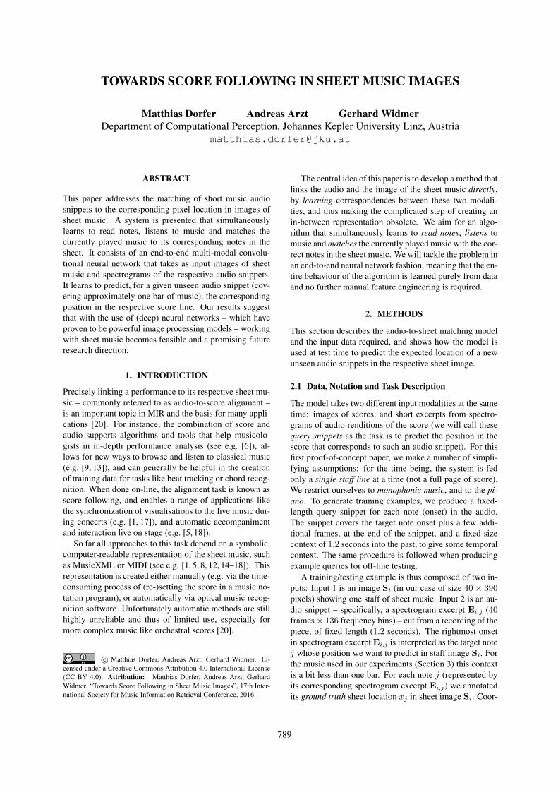
Figure 5 shows the image of one staff of sheet music alongwith the predicted as well as the ground truth pixel locationfor a snippet of audio. The network correctly matches thespectrogram with the corresponding pixel location in thesheet image. However, we observe a second peak in thebucket prediction probability vector. A closer look showsthat this is entirely reasonable, as the music is quite repet-itive and the current target situation actually appears twicein the score. The ability of predicting probabilities formultiple positions is a desirable and important property, asrepetitive structures are immanent to music. The resultingprediction ambiguities can be addressed by exploiting thetemporal relations between the notes in a piece by meth-ods such as dynamic time warping or probabilistic models.In fact, we plan to combine the probabilistic output of ourmatching model with existing score following methods, asfor example [2]. In Section 2 we mentioned that training asheet location prediction with MSE-regression is difficultto optimize. Besides this technical drawback it would notbe straightforward to predict a variable number of locationswith an MSE-model, as the number of network outputs hasto be fixed when designing the model.

In addition to the network inputs and prediction Fig. 5also shows a saliency map [19] computed on the inputsheet image with respect to the network output. 5 Thesaliency can be interpreted as the input regions to whichmost of the net’s attention is drawn. In other words, it high-lights the regions that contribute most to the current outputproduced by the model. A nice insight of this visualiza-tion is that the network actually focuses and recognizes theheads of the individual notes. In addition it also directssome attention to the style of stems, which is necessary todistinguish for example between quarter and eighth notes.

5 The implementation is adopted from an example by Jan Schluter inthe recipes section of the deep learning framework Lasagne [7].

Proceedings of the 17th ISMIR Conference, New York City, USA, August 7-11, 2016 793

Staff ImageSpectrogram

Saliency (Staff Image)

0 5 10 15 20 25 30 35Bucket

0.00.20.40.60.81.0

Proba

bility

Bucket­Distance: 0

ground truthprediction

Figure 5: Example prediction of the proposed model. The top row shows the input staff image Si along with the bucket borders as thingray lines, and the given query audio (spectrogram) snippet Ei,j . The plot in the middle visualizes the salience map (representing theattention of the neural network) computed on the input image. Note that the network’s attention is actually drawn to the individual noteheads. The bottom row compares the ground truth bucket probabilities with the probabilities predicted by the network. In addition, wealso highlight the corresponding true and predicted pixel locations in the staff image in the top row.

The optimization on soft target vectors is also reflectedin the predicted bucket probabilities. In particular theneighbours of the bucket with maximum activation are alsoactive even though there is no explicit neighbourhood re-lation encoded in the soft-max output layer. This helps theinterpolation of the true position in the image (see Fig. 4).

4.2 First Steps with Real Music

As a final point, we report on first attempts at working with“real” music. For this purpose one of the authors playedthe right hand part of a simple piece (Minuet in G Majorby Johann Sebastian Bach, BWV Anhang 114) – which,of course, was not part of the training data – on a YamahaAvantGrand N2 hybrid piano and recorded it using a sin-gle microphone. In this application scenario we predictthe corresponding sheet locations not only at times of on-sets but for a continuous audio stream (subsequent spec-trogram excerpts). This can be seen as a simple versionof online score following in sheet music, without takinginto account the temporal relations of the predictions. Weoffer the reader a video 6 that shows our model followingthe first three staff lines of this simple piece. 7 The ra-tio of predicted notes having a pixel-distance smaller thanthe bucket width (compare Section 3.5) is 71.72% for this

6 https://www.dropbox.com/s/0nz540i1178hjp3/Bach_Minuet_G_Major_net4b.mp4?dl=0

7 Note: our model operates on single staffs of sheet music and requiresa certain context of spectrogram frames for prediction (in our case 40frames). For this reason it cannot provide a localization for the first coupleof notes in the beginning of each staff at the current stage. In the videoone can observe that prediction only starts when the spectrogram in thetop right corner has grown to the desired size of 40 frames. We kept thisbehaviour for now as we see our work as a proof of concept. The issuecan be easily addressed by concatenating the images of subsequent staffsin horizontal direction. In this way we will get a “continuous stream ofsheet music” analogous to a spectrogram for audio.

real recording. This corresponds to a average normalized-pixel-distance of 0.0402.

5. CONCLUSION

In this paper we presented a multi-modal convolutionalneural network which is able to match short snippets ofaudio with their corresponding position in the respectiveimage of sheet music, without the need of any symbolicrepresentation of the score. First evaluations on simple pi-ano music suggest that this is a very promising new ap-proach that deserves to be explored further.

As this is a proof of concept paper, naturally our methodstill has some severe limitations. So far our approach canonly deal with monophonic music, notated on a singlestaff, and with performances that are roughly played in thesame tempo as was set in our training examples.

In the future we will explore options to lift these limi-tations one by one, with the ultimate goal of making thisapproach applicable to virtually any kind of complex sheetmusic. In addition, we will try to combine this approachwith a score following algorithm. Our vision here is tobuild a score following system that is capable of dealingwith any kind of classical sheet music, out of the box, withno need for data preparation.

6. ACKNOWLEDGEMENTS

This work is supported by the Austrian Ministries BMVITand BMWFW, and the Province of Upper Austria via theCOMET Center SCCH, and by the European ResearchCouncil (ERC Grant Agreement 670035, project CONESPRESSIONE). The Tesla K40 used for this research wasdonated by the NVIDIA corporation.

794 Proceedings of the 17th ISMIR Conference, New York City, USA, August 7-11, 2016

7. REFERENCES

[1] Andreas Arzt, Harald Frostel, Thassilo Gadermaier,Martin Gasser, Maarten Grachten, and Gerhard Wid-mer. Artificial intelligence in the concertgebouw. InProceedings of the International Joint Conferenceon Artificial Intelligence (IJCAI), Buenos Aires, Ar-gentina, 2015.

[2] Andreas Arzt, Gerhard Widmer, and Simon Dixon. Au-tomatic page turning for musicians via real-time ma-chine listening. In Proc. of the European Conferenceon Artificial Intelligence (ECAI), Patras, Greece, 2008.

[3] Sebastian Bock, Filip Korzeniowski, Jan Schluter, Flo-rian Krebs, and Gerhard Widmer. madmom: a newPython Audio and Music Signal Processing Library.arXiv:1605.07008, 2016.

[4] Nicolas Boulanger-lewandowski, Yoshua Bengio, andPascal Vincent. Modeling temporal dependencies inhigh-dimensional sequences: Application to poly-phonic music generation and transcription. In Proceed-ings of the 29th International Conference on MachineLearning (ICML-12), pages 1159–1166, 2012.

[5] Arshia Cont. A coupled duration-focused architecturefor realtime music to score alignment. IEEE Transac-tions on Pattern Analysis and Machine Intelligence,32(6):837–846, 2009.

[6] Nicholas Cook. Performance analysis and chopin’smazurkas. Musicae Scientae, 11(2):183–205, 2007.

[7] Sander Dieleman, Jan Schluter, Colin Raffel, Eben Ol-son, Søren Kaae Sønderby, Daniel Nouri, Eric Batten-berg, Aaron van den Oord, et al. Lasagne: First re-lease., August 2015.

[8] Zhiyao Duan and Bryan Pardo. A state space model foron-line polyphonic audio-score alignment. In Proc. ofthe IEEE Conference on Acoustics, Speech and SignalProcessing (ICASSP), Prague, Czech Republic, 2011.

[9] Jon W. Dunn, Donald Byrd, Mark Notess, Jenn Ri-ley, and Ryan Scherle. Variations2: Retrieving and us-ing music in an academic setting. Communications ofthe ACM, Special Issue: Music information retrieval,49(8):53–48, 2006.

[10] Xavier Glorot, Antoine Bordes, and Yoshua Bengio.Deep sparse rectifier neural networks. In InternationalConference on Artificial Intelligence and Statistics,pages 315–323, 2011.

[11] Sergey Ioffe and Christian Szegedy. Batch normaliza-tion: Accelerating deep network training by reducinginternal covariate shift. CoRR, abs/1502.03167, 2015.

[12] Ozgur Izmirli and Gyanendra Sharma. Bridgingprinted music and audio through alignment using amid-level score representation. In Proceedings of the13th International Society for Music Information Re-trieval Conference, Porto, Portugal, 2012.

[13] Mark S. Melenhorst, Ron van der Sterren, AndreasArzt, Agustın Martorell, and Cynthia C. S. Liem. Atablet app to enrich the live and post-live experience ofclassical concerts. In Proceedings of the 3rd Interna-tional Workshop on Interactive Content Consumption(WSICC) at TVX 2015, 06/2015 2015.

[14] Marius Miron, Julio Jose Carabias-Orti, and JordiJaner. Audio-to-score alignment at note level for or-chestral recordings. In Proc. of the InternationalConference on Music Information Retrieval (ISMIR),Taipei, Taiwan, 2014.

[15] Meinard Muller, Frank Kurth, and Michael Clausen.Audio matching via chroma-based statistical features.In Proc. of the International Society for Music Infor-mation Retrieval Conference (ISMIR), London, GreatBritain, 2005.

[16] Bernhard Niedermayer and Gerhard Widmer. A multi-pass algorithm for accurate audio-to-score alignment.In Proc. of the International Society for Music In-formation Retrieval Conference (ISMIR), Utrecht, TheNetherlands, 2010.

[17] Matthew Prockup, David Grunberg, Alex Hrybyk, andYoungmoo E. Kim. Orchestral performance compan-ion: Using real-time audio to score alignment. IEEEMultimedia, 20(2):52–60, 2013.

[18] Christopher Raphael. Music Plus One and machinelearning. In Proceedings of the International Confer-ence on Machine Learning (ICML), 2010.

[19] Jost Tobias Springenberg, Alexey Dosovitskiy,Thomas Brox, and Martin Riedmiller. Striving for sim-plicity: The all convolutional net. arXiv:1412.6806,2014.

[20] Verena Thomas, Christian Fremerey, Meinard Muller,and Michael Clausen. Linking Sheet Music and Au-dio - Challenges and New Approaches. In MeinardMuller, Masataka Goto, and Markus Schedl, editors,Multimodal Music Processing, volume 3 of DagstuhlFollow-Ups, pages 1–22. Schloss Dagstuhl–Leibniz-Zentrum fuer Informatik, Dagstuhl, Germany, 2012.

Proceedings of the 17th ISMIR Conference, New York City, USA, August 7-11, 2016 795