Towards PDE-Based Image Compression

Irena Galic1,2, Joachim Weickert1, Martin Welk1,Andres Bruhn1, Alexander Belyaev2, and Hans-Peter Seidel2

1 Mathematical Image Analysis Group, Faculty of Math. and Computer Science,Saarland University, Building 27, 66041 Saarbrucken, Germany

galic, weickert, welk, bruhn@mia.uni-saarland.de2 Max-Planck Institute for Informatics, Stuhlsatzenhausweg 85,

66123 Saarbrucken, Germanybelyaev, hpseidel@mpi-sb.mpg.de

Abstract. While methods based on partial differential equations (PDEs) andvariational techniques are powerful tools for denoising and inpainting digital im-ages, their use for image compression was mainly focussing on pre- or post-processing so far. In our paper we investigate their potential within the decod-ing step. We start with the observation that edge-enhancing diffusion (EED), ananisotropic nonlinear diffusion filter with a diffusion tensor, is well-suited forscattered data interpolation: Even when the interpolation data are very sparse,good results are obtained that respect discontinuities and satisfy a maximum–minimum principle. This property is exploited in our studies on PDE-based imagecompression. We use an adaptive triangulation method based on B-tree coding forremoving less significant pixels from the image. The remaining points serve asscattered interpolation data for the EED process. They can be coded in a compactand elegant way that reflects the B-tree structure. Our experiments illustrate thatfor high compression rates and non-textured images, this PDE-based approachgives visually better results than the widely-used JPEG coding.

1 Introduction

In recent years several partial differential equations (PDEs) and variational techniqueshave shown their usefulness in so-called inpainting methods [19,2,4,13,27]. Here oneaims at filling in missing informations in certain corrupted image areas by means of sec-ond or higher-order PDES. The basic idea is to regard the given image data as Dirichletboundary conditions, and interpolate the data in the inpainting regions by solving appro-priate boundary value problems. Related variational and PDE methods have also beeninvestigated for more classical interpolation problems such as zooming into an imageby increasing its resolution [3,18]. For such interpolation problems with data given ona regular grid, these techniques are in competition with cubic or quintic splines, radialbasis functions and sinc-based interpolation techniques; see e.g. [17,20]. If the data arenot available on a regular grid, scattered data interpolation techniques have been pro-posed [11,22], among which radial basis functions such as thin plate splines [9] arepopular and well-performing.

Interestingly, not many of the variational and PDE-based interpolation and inpaint-ing techniques have been used for scattered data interpolation. It seems that the sparsity

N. Paragios et al. (Eds.): VLSM 2005, LNCS 3752, pp. 37–48, 2005.c© Springer-Verlag Berlin Heidelberg 2005

38 I. Galic et al.

of the scattered data constitutes a real challenge for these techniques: While second-order PDEs may satisfy a maximum–minimum principle, they often create singularitiesat isolated interpolation points in 2-D. Higher-order PDEs, on the other hand, may givesmoother solutions, but the violation of an extremum principle can lead to undesirableover- and undershoots; see e.g [3].

The goal of the present paper is twofold: First we address the before mentionedproblem by investigating a partial differential equation that has not been consideredfor interpolation problems before, namely edge-enhancing anisotropic diffusion (EED)[28]. It uses a diffusion tensor that allows smoothing along discontinuities while inhibit-ing smoothing across them. In our experiments we will see that this technique performsfavourably in the context of scattered data interpolation. A second goal of our paper isto investigate if this property can be used for lossy image compression. While contem-porary image compression methods are dominated by concepts that involve the discretecosine transform (such as the widely-used JPEG standard [23]) or the discrete wavelettransform (in JPEG2000 [26]), our goal is to give a proof-of-concept that there are al-ternatives where PDEs may be beneficial. The basic idea is to reduce the image data toa well-adapted set of significant sparse points that can be coded in an efficient way. De-coding is accomplished by using these scattered data and interpolating them by meansof edge-enhancing anisotropic diffusion. As a tool for creating a useful sparse pointrepresentation, we consider the B-tree triangular coding (BTTC) by Distasi et al. [8],since it is relatively simple and allows an efficient coding of the sparsified image data.

Our paper is organised as follows. In Section 2 we describe PDE-based interpolationtechniques and show that scattered data interpolation with EED performs particularlywell. In Section 3 we review the BTTC model for image coding and describe how it canbe coupled with PDE-based interpolation. Experiments on EED-based image codingare presented in Section 4, and the paper is concluded with a summary in Section 5.

Related Work. In the context of image compression, PDEs and related variational tech-niques have mainly been used as a preprocessing step before coding [10,16] or as a post-processing tool for removing coding artifacts [1,12,21,29,30]. Our works differs fromthese papers by the fact that we use PDEs within the decoding step rather than as pre- orpostprocessing tools. Chan and Zhou [5] used total variation regularisation in order tomodify the coefficients in a wavelet decomposition such that oscillatory edge artifactsare reduced, while Sole et al. [25] investigate three PDEs for interpolating structures indigital elevation maps and report the most favourable results with the Laplacian oper-ator. An interesting coding scheme that exploits scattered data interpolation has beenproposed by Demaret et al. [7]. They construct an adaptive Delaunay triangulation thatis used for decoding the image by linear interpolation. Their experiments show that itcan be an alternative to JPEG 2000 coding for texture-free images.

2 PDE-Based Interpolation

We start by considering a PDE approach to image interpolation. First we discuss a gen-eral model, then we investigate four possibilities for smoothing operators, and finallywe present an experiment that illustrates their properties.

Towards PDE-Based Image Compression 39

2.1 General Model

Let Ω ⊂ IRn denote an n-dimensional image domain. We want to recover some un-known scalar-valued function v : Ω → IR, from which we know its values on somesubset Ω1 ⊂ Ω. Our goal is to find an interpolating function u : Ω → IR that is smoothand close to v in Ω \ Ω1 and identical to v in Ω1.

We may embed this problem in an evolution setting with some evolution parameter(the ”time”) t ≥ 0. It solution u(x, t) gives the desired interpolating function as itssteady state (t → ∞). We initialise the evolution with some function f : Ω → IR thatis identical to v on Ω1 and that is set to some arbitrary value (e.g. to 0) on Ω \ Ω1:

f(x) :=

v(x) if x ∈ Ω10 else.

(1)

We consider the evolution

∂tu = (1−c(x))Lu − c(x) (u − f) (2)

with f as initial value,u(x, 0) = f(x), (3)

and reflecting (homogeneous Neumann) boundary conditions on the image boundary∂Ω. The function c : Ω → IR is the characteristic function on Ω1, i.e.

c(x) :=

1 if x ∈ Ω10 else,

(4)

and L is some elliptic differential operator. The idea is to solve the steady state equation

(1−c(x))Lu − c(x) (u − f) = 0 (5)

with reflecting boundary conditions. In Ω1 we have c(x) = 1 such that the interpolationcondition u(x) = f(x) = v(x) is fulfilled. In Ω \ Ω1 it follows from c(x) = 0 that thesolution has to satisfy Lu = 0. This elliptic PDE can be regarded as the steady state ofthe evolution equation

∂tu = Lu (6)

with Dirichlet boundary conditions given by the interpolation data on Ω1.

2.2 Specific Smoothing Operators

Regarding the elliptic differential operator L, many possibilities exist. The simplest oneuses the Laplacian Lu := ∆u leading to homogeneous diffusion [15]:

∂tu = ∆u. (7)

A prototype for a higher order differential operator is the biharmonic operator Lu :=−∆2u giving the biharmonic smoothing evolution

∂tu = −∆2u. (8)

Using it for interpolation comes down to thin plate spline interpolation [9], a rotationallyinvariant multidimensional generalisations of cubic spline interpolation. Note that only

40 I. Galic et al.

the second-order differential operators allow a maximum–minimum principle, wherethe values of u stay within the range of the values of f in Ω1.

Nonlinear isotropic diffusion processes are governed by Lu := div (g(|∇u|2)∇u).This gives [24]

∂tu = div (g(|∇u|2)∇u) (9)

where the diffusivity function g is decreasing in its argument, since the goal is to re-duce smoothing at edges where |∇u| is large. One may e.g. choose the Charbonnierdiffusivity [6]

g(s2) =1√

1 + s2/λ2(10)

with some contrast parameter λ > 0. Since (9) uses a scalar-valued diffusivity we namethis process isotropic (in contrast to the nomenclature in [24]).

Real anisotropic behaviour is possible when a diffusion tensor is used. As a proto-type for nonlinear anisotropic diffusion filtering we consider edge-enhancing diffusion(EED) [28]. The idea is to reduce smoothing across edges while still permitting diffu-sion along them. The EED diffusion tensor has one eigenvector parallel to ∇uσ, whereuσ is obtained from convolving u with a Gaussian with standard deviation σ. The corre-sponding eigenvalue is given by g(|∇uσ|2) with a diffusivity function such as (10). Theother eigenvectors are orthogonal to ∇uσ and have corresponding eigenvalues 1. If weuse the convention to extend a scalar-valued function g(x) to a matrix-valued functiong(A) by applying g to the eigenvalues on A and leaving the eigenvectors unchanged,then EED can be formally linked to Lu := div (g(∇uσ∇u

σ )∇u). Hence, its evolutionis governed by

∂tu = div (g(∇uσ∇uσ )∇u). (11)

2.3 Experiments on Interpolation

In order to evaluate the potential of the preceding PDEs for scattered data interpola-tion, we have discretised them with central finite differences in space. For the diffusionequations, we performed a semi-implicit time discretisation with SOR as solver for thelinear systems of equations, while for biharmonic smoothing an explicit scheme wasused. Runtimes for a non-optimised C implementation on a 1.5 GHz Centrino laptoprange between a few seconds and several minutes for a 256 × 256 image.

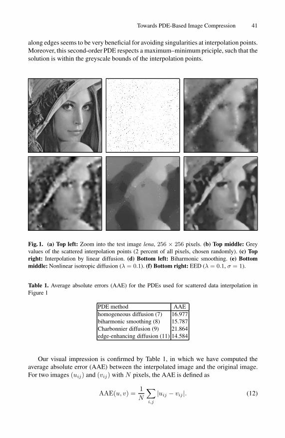
In Figure 1 we present an experiment that illustrates the use of the different smooth-ing operators for scattered data interpolation. It depicts a zoom into the famous lenaimage, where 2 percent of all pixels have been chosen randomly as scattered interpo-lation points. We observe that homogeneous diffusion is not very suitable for scattereddata interpolation, since it creates singularities at the interpolation points. This can beavoided with interpolation using biharmonic smoothing. It gives fairly good results, butsuffers from over- and undershoots near edges due to the violation of an extremum prin-ciple (see e.g. the shoulder). Interestingly, going from homogeneous diffusion to non-linear isotropic diffusion does not give an improvement: Although nonlinear isotropicdiffusion may allow discontinuities, its interpolant is too flat and tends to keep manyinterpolation points as isolated singularities. The fact that EED, on the other hand, givesthe best results shows the importance of the anisotropic behaviour. Its ability to smooth

Towards PDE-Based Image Compression 41

along edges seems to be very beneficial for avoiding singularities at interpolation points.Moreover, this second-order PDE respects a maximum–minimum priciple, such that thesolution is within the greyscale bounds of the interpolation points.

Fig. 1. (a) Top left: Zoom into the test image lena, 256 × 256 pixels. (b) Top middle: Greyvalues of the scattered interpolation points (2 percent of all pixels, chosen randomly). (c) Topright: Interpolation by linear diffusion. (d) Bottom left: Biharmonic smoothing. (e) Bottommiddle: Nonlinear isotropic diffusion (λ = 0.1). (f) Bottom right: EED (λ = 0.1, σ = 1).

Table 1. Average absolute errors (AAE) for the PDEs used for scattered data interpolation inFigure 1

PDE method AAEhomogeneous diffusion (7) 16.977biharmonic smoothing (8) 15.787Charbonnier diffusion (9) 21.864edge-enhancing diffusion (11) 14.584

Our visual impression is confirmed by Table 1, in which we have computed theaverage absolute error (AAE) between the interpolated image and the original image.For two images (uij) and (vij) with N pixels, the AAE is defined as

AAE(u, v) =1N

∑i,j

|uij − vij |. (12)

42 I. Galic et al.

Nonlinear isotropic diffusion performes worst, followed by homogeneous diffusion andbiharmonic smoothing, while EED gives the smallest interpolation error. This showsthat for scattered data interpolation, EED is a very promising PDE that has not beeninvestigated in this context before.

3 Image Coding by Binary Trees

Now that we have seen that EED is useful for scattered data interpolation, we want toexploit this technique for image compression. To this end we have to couple it with amethod that provides a useful sparse image representation with scattered data.

3.1 Creating Scattered Interpolation Points

Our image compression and decompression scheme relies on an adaptive sparsificationof the image data by means of the triangulation from B-tree triangular coding (BTTC)[8]. In this coding, an image is decomposed into a number of triangular regions suchthat within each region it can be recovered in sufficient quality by interpolation from thevertices. In our case, all regions are isosceles rectangular triangles. The decompositioninto triangles then is stored in a binary tree structure.

In order to describe the compression procedure, let us assume we have an imagev = (vij) of size (2m +1)× (2m +1). Smaller images should be filled up to such a sizein a suitable way. Initially, the image is split by one of its diagonals into two triangles.The four image corners (1, 1), (1, 2m+1), (2m+1, 1) and (2m+1, 2m+1) are verticesof these two triangles.

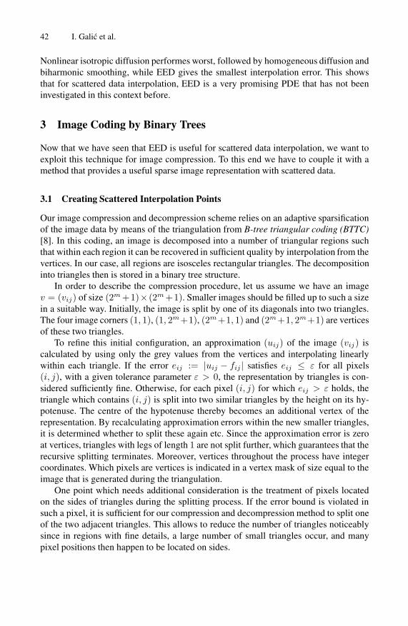
To refine this initial configuration, an approximation (uij) of the image (vij) iscalculated by using only the grey values from the vertices and interpolating linearlywithin each triangle. If the error eij := |uij − fij | satisfies eij ≤ ε for all pixels(i, j), with a given tolerance parameter ε > 0, the representation by triangles is con-sidered sufficiently fine. Otherwise, for each pixel (i, j) for which eij > ε holds, thetriangle which contains (i, j) is split into two similar triangles by the height on its hy-potenuse. The centre of the hypotenuse thereby becomes an additional vertex of therepresentation. By recalculating approximation errors within the new smaller triangles,it is determined whether to split these again etc. Since the approximation error is zeroat vertices, triangles with legs of length 1 are not split further, which guarantees that therecursive splitting terminates. Moreover, vertices throughout the process have integercoordinates. Which pixels are vertices is indicated in a vertex mask of size equal to theimage that is generated during the triangulation.

One point which needs additional consideration is the treatment of pixels locatedon the sides of triangles during the splitting process. If the error bound is violated insuch a pixel, it is sufficient for our compression and decompression method to split oneof the two adjacent triangles. This allows to reduce the number of triangles noticeablysince in regions with fine details, a large number of small triangles occur, and manypixel positions then happen to be located on sides.

Towards PDE-Based Image Compression 43

3.2 Coding

To efficiently store the triangulation, we notice that the hierarchical splitting of trian-gles gives rise to a binary tree structure. Each triangle occurring during the splittingprocess is represented by a node while leaves correspond to those triangles which arenot divided further. When a triangle is split, its two subtriangles become the childrenof its representing node. To store the structure of the tree, one traverses the tree andstores one bit per node: a 1 for a node that has children, and a 0 for a leave. Preorderor level-order traversal are equally possible. Note that by the tree structure, the vertexmask is fully determined. Further space in storing the tree is saved by measuring glob-ally the minimal and maximal depth of the tree. Only for nodes at intermediate levels,the corresponding bits are stored.

For coding the grey values in all vertices, we first zig zag traverse the sparse im-age created with the binary tree structure and store it in a sequence of grey values.This sequence is then compressed with Huffman coding [14], a lossless variable-lengthprefix code that assigns smaller codes to more frequent characters. It also uses a treestructure.

Our entire coded image format then reads as follows:

– image size (4 bytes)– minimal and maximal depth of the binary tree (together 2 bytes)– binary string encoding binary tree structure (1 bit for each node between minimal

and maximal depth, filled up with zeros to the next byte boundary)– first grey-value in a sequence of grey values (1 byte)– minimal and maximal depth of the Huffman coded binary tree (2 bytes)– binary string for Huffman-coded binary tree (1 bit for each node between minimal

and maximal depth, filled up with zeros to the next byte boundary)– Huffman dictionary (less than 256 bytes)– sequence of Huffman-coded grey values

We further enhanced this coding by a (lossy) requantisation step that reduced thenumber of grey values in the initial image from 256 to 64.

3.3 Decoding

Decompression takes place in two steps. In the first step, the vertex mask is recoveredfrom the binary tree representation, and the stored grey values are placed at the ap-propriate pixel positions to give the sparse image. To recover the vertex mask, the treeis generated in the same order as it was stored. Along with generating nodes, vertexpositions are calculated and marked in the vertex mask.

The second step consists in the interpolation of the image, where the vertex maskbecomes the interpolation mask. In the BTTC scheme of Distasi et al. [8], linear in-terpolation within each traingle is used. In the sequel we will denote this technique byBTTC-L.

Since we have already seen that EED performs favourably as a scattered data in-terpolant, it is natural to renounce the linear interpolation step in the BTTC-L methodand apply EED to the interpolation mask that has been created by the BTTC method.

44 I. Galic et al.

We abbreviate this novel method by BTTC-EED. Note that in contrast to BTTC-L,BTTC-EED does not rely on the triangulation, only on its vertices as interpolationpoints.

4 Experiments on Compression

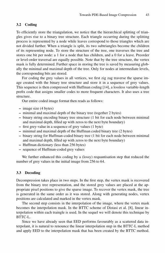
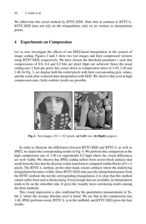
Let us now investigate the effects of our EED-based interpolation in the context ofimage coding. Figures 2 and 3 show two test images and their compressed versionsusing BTTC-EED, respectively. We have chosen the threshold parameter ε such thatcompressions of 0.8, 0.4 and 0.2 bits per pixel (bpp) are achieved. Since the usualcoding uses 1 byte per pixel, this comes down to compression ratios of 1:10, 1:20 and1:40. In Fig. 3, we display both the coded pixels with their corresponding grey values,and the result after scattered data interpolation with EED. We observe that even at highcompression rates, fairly realistic results are possible.

Fig. 2. Test images, 257 × 257 pixels. (a) Left: trui. (b) Right: peppers.

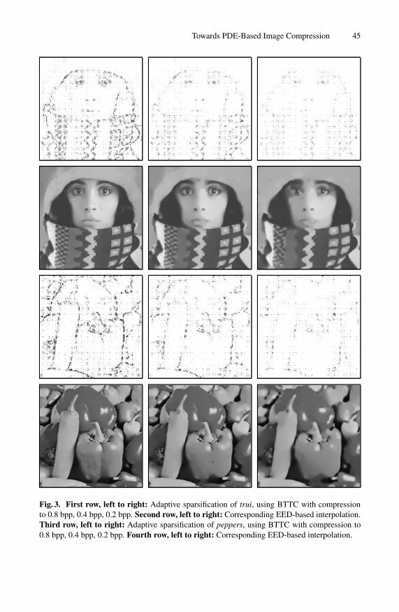
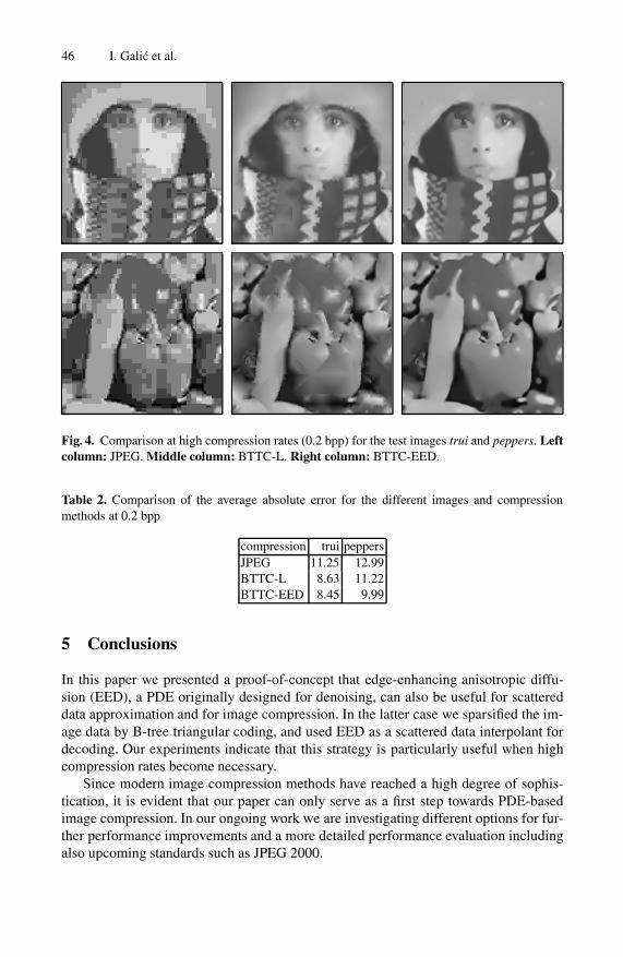
In order to illustrate the differences between BTTC-EED and BTTC-L as well asJPEG, we depict the corresponding results in Fig. 4. We perform this comparison at thehigh compression rate of 1:40 (or equivalently 0.2 bpp) where the visual differencesare well visible. We observe that JPEG coding suffers from severe block artifacts thatresult from the fact that the discrete cosine transform is computed within blocks of 8×8pixels. The BTTC-L method, on the other hand, creates artifacts where the underlyingtriangulation becomes visible. Since BTTC-EED only uses the interpolation points fromthe BTTC method, but not the corresponding triangulation, it is clear that this methodcannot suffer from such a shortcoming. If not enough data are available, its interpolationtends to be on the smoother side. It gives the visually most convincing results amongthe three methods.

This visual impression is also confirmed by the quantitative measurements in Ta-ble 2, where the average absolute error is listed. We see that at the compression rate1:40, JPEG performs worst, BTTC-L is in the midfield, and BTTC-EED gives the bestresults.

Towards PDE-Based Image Compression 45

Fig. 3. First row, left to right: Adaptive sparsification of trui, using BTTC with compressionto 0.8 bpp, 0.4 bpp, 0.2 bpp. Second row, left to right: Corresponding EED-based interpolation.Third row, left to right: Adaptive sparsification of peppers, using BTTC with compression to0.8 bpp, 0.4 bpp, 0.2 bpp. Fourth row, left to right: Corresponding EED-based interpolation.

46 I. Galic et al.

Fig. 4. Comparison at high compression rates (0.2 bpp) for the test images trui and peppers. Leftcolumn: JPEG. Middle column: BTTC-L. Right column: BTTC-EED.

Table 2. Comparison of the average absolute error for the different images and compressionmethods at 0.2 bpp

compression trui peppersJPEG 11.25 12.99BTTC-L 8.63 11.22BTTC-EED 8.45 9.99

5 Conclusions

In this paper we presented a proof-of-concept that edge-enhancing anisotropic diffu-sion (EED), a PDE originally designed for denoising, can also be useful for scattereddata approximation and for image compression. In the latter case we sparsified the im-age data by B-tree triangular coding, and used EED as a scattered data interpolant fordecoding. Our experiments indicate that this strategy is particularly useful when highcompression rates become necessary.

Since modern image compression methods have reached a high degree of sophis-tication, it is evident that our paper can only serve as a first step towards PDE-basedimage compression. In our ongoing work we are investigating different options for fur-ther performance improvements and a more detailed performance evaluation includingalso upcoming standards such as JPEG 2000.

Towards PDE-Based Image Compression 47

Acknowledgements. Our research is partly funded by the International Max-PlanckResearch School (IMPRS). This is gratefully acknowledged. Joachim Weickert alsothanks Vicent Caselles for interesting discussions on EED-based interpolation duringa stay at the University Pompeu Fabra, Barcelona.

References

1. F. Alter, S. Durand, and J. Froment. Adapted total variation for artifact free decompressionof JPEG images. Journal of Mathematical Imaging and Vision, 23(2):199–211, September2005.

2. M. Bertalmıo, G. Sapiro, V. Caselles, and C. Ballester. Image inpainting. In Proc. SIG-GRAPH 2000, pages 417–424, New Orleans, LI, July 2000.

3. V. Caselles, J.-M. Morel, and C. Sbert. An axiomatic approach to image interpolation. IEEETransactions on Image Processing, 7(3):376–386, March 1998.

4. T. F. Chan and J. Shen. Non-texture inpainting by curvature-driven diffusions (CDD). Jour-nal of Visual Communication and Image Representation, 12(4):436–449, 2001.

5. T. F. Chan and H. M. Zhou. Total variation improved wavelet thresholding in image com-pression. In Proc. Seventh International Conference on Image Processing, volume II, pages391–394, Vancouver, Canada, September 2000.

6. P. Charbonnier, L. Blanc-Feraud, G. Aubert, and M. Barlaud. Deterministic edge-preservingregularization in computed imaging. IEEE Transactions on Image Processing, 6(2):298–311,1997.

7. L. Demaret, N. Dyn, and A. Iske. Image compression by linear splines over adaptive tri-angulations. Technical report, Dept. of Mathematics, University of Leicester, UK, January2005.

8. R. Distasi, M. Nappi, and S. Vitulano. Image compression by B-tree triangular coding. IEEETransactions on Communications, 45(9):1095–1100, 1997.

9. J. Duchon. Interpolation des fonctions de deux variables suivant le principe de la flexion desplaques minces. RAIRO Mathematical Models and Numerical Analysis, 10:5–12, 1976.

10. G. E. Ford, R. R. Estes, and H. Chen. Scale-space analysis for image sampling and interpo-lation. In Proc. IEEE International Conference on Acoustics, Speech and Signal Processing,volume 3, pages 165–168, San Francisco, CA, March 1992.

11. R. Franke. Scattered data interpolation: Tests of some methods. Mathematics of Computa-tion, 38:181–200, 1982.

12. A. Gothandaraman, R. Whitaker, and J. Gregor. Total variation for the removal of blockingeffects in DCT based encoding. In Proc. 2001 IEEE International Conference on ImageProcessing, volume 2, pages 455–458, Thessaloniki, Greece, October 2001.

13. H. Grossauer and O. Scherzer. Using the complex Ginzburg–Landau equation for digitalimpainting in 2D and 3D. In L. D. Griffin and M. Lillholm, editors, Scale-Space Methodsin Computer Vision, volume 2695 of Lecture Notes in Computer Science, pages 225–236,Berlin, 2003. Springer.

14. D. A. Huffman. A method for the construction of minimum redundancy codes. Proceedingsof the IRE, 40:1098–1101, 1952.

15. T. Iijima. Basic theory on normalization of pattern (in case of typical one-dimensional pat-tern). Bulletin of the Electrotechnical Laboratory, 26:368–388, 1962. In Japanese.

16. I. Kopilovic and T. Sziranyi. Artifact reduction with diffusion preprocessing for image com-pression. Optical Engineering, 44(2):1–14, February 2005.

17. T. Lehmann, C. Gonner, and K. Spitzer. Survey: Interpolation methods in medical imageprocessing. IEEE Transactions on Medical Imaging, 18(11):1049–1075, November 1999.

48 I. Galic et al.

18. F. Malgouyres and F. Guichard. Edge direction preserving image zooming: A mathematicaland numerical analysis. SIAM Journal on Numerical Analysis, 39(1):1–37, 2001.

19. S. Masnou and J.-M. Morel. Level lines based disocclusion. In Proc. 1998 IEEE Inter-national Conference on Image Processing, volume 3, pages 259–263, Chicago, IL, October1998.

20. E. Meijering. A chronology of interpolation: From ancient astronomy to modern signal andimage processing. Proceedings of the IEEE, 90(3):319–342, March 2002.

21. P. Mrazek. Nonlinear Diffusion for Image Filtering and Monotonicity Enhancement. PhDthesis, Czech Technical University, Prague, Czech Republic, June 2001.

22. G. M. Nielson and J. Tvedt. Comparing methods of interpolation for scattered volumetricdata. In D. F. Rogers and R. A. Earnshaw, editors, State of the Art in Computer Graphics:Aspects of Visualization, pages 67–86. Springer, New York, 1994.

23. W. B. Pennebaker and J. L. Mitchell. JPEG: Still Image Data Compression Standard.Springer, New York, 1992.

24. P. Perona and J. Malik. Scale space and edge detection using anisotropic diffusion. IEEETransactions on Pattern Analysis and Machine Intelligence, 12:629–639, 1990.

25. A. Sole, V. Caselles, G. Sapiro, and F. Arandiga. Morse description and geometric encod-ing of digital elevation maps. IEEE Transactions on Image Processing, 13(9):1245–1262,September 2004.

26. D. S. Taubman and M. W. Marcellin, editors. JPEG 2000: Image Compression Fundamen-tals, Standards and Practice. Kluwer, Boston, 2002.

27. D. Tschumperle and R. Deriche. Vector-valued image regularization with PDEs: A commonframework for different applications. IEEE Transactions on Pattern Analysis and MachineIntelligence, 27(4):506–516, April 2005.

28. J. Weickert. Theoretical foundations of anisotropic diffusion in image processing. ComputingSupplement, 11:221–236, 1996.

29. S. Yang and Y.-H. Hu. Coding artifact removal using biased anisotropic diffusion. InProc. 1997 IEEE International Conference on Image Processing, volume 2, pages 346–349,Santa Barbara, CA, October 1997.

30. S. Yao, W. Lin, Z. Lu, E. P. Ong, and X. Yang. Adaptive nonlinear diffusion processes forringing artifacts removal on JPEG 2000 images. In Proc. 2004 IEEE International Confer-ence on Multimedia and Expo, pages 691–694, Taipei, Taiwan, June 2004.