Towards Calibration Of Optical Flow Of Crowd Videos Using

University of Central Florida University of Central Florida

STARS STARS

Electronic Theses and Dissertations, 2004-2019

2011

Towards Calibration Of Optical Flow Of Crowd Videos Using Towards Calibration Of Optical Flow Of Crowd Videos Using

Observed Trajectories Observed Trajectories

Iman K. Elbadramany University of Central Florida

Part of the Computer Engineering Commons

Find similar works at: https://stars.library.ucf.edu/etd

University of Central Florida Libraries http://library.ucf.edu

This Masters Thesis (Open Access) is brought to you for free and open access by STARS. It has been accepted for

inclusion in Electronic Theses and Dissertations, 2004-2019 by an authorized administrator of STARS. For more

information, please contact [email protected].

STARS Citation STARS Citation Elbadramany, Iman K., "Towards Calibration Of Optical Flow Of Crowd Videos Using Observed Trajectories" (2011). Electronic Theses and Dissertations, 2004-2019. 1923. https://stars.library.ucf.edu/etd/1923

https://stars.library.ucf.edu/



https://stars.library.ucf.edu/etd

http://network.bepress.com/hgg/discipline/258?utm_source=stars.library.ucf.edu%2Fetd%2F1923&utm_medium=PDF&utm_campaign=PDFCoverPages

https://stars.library.ucf.edu/etd

http://library.ucf.edu/

mailto:[email protected]

https://stars.library.ucf.edu/etd/1923?utm_source=stars.library.ucf.edu%2Fetd%2F1923&utm_medium=PDF&utm_campaign=PDFCoverPages



TOWARDS CALIBRATION OF OPTICAL FLOW OF CROWD VIDEOS

USING OBSERVED TRAJECTORIES

by

IMAN K. ELBADRAMANY B.Sc. The American University in Cairo. 1979

A thesis submitted in partial fulfillment of the requirements for the degree of Master of Science in Modeling and Simulation

in the College of Sciences at the University of Central Florida

Orlando, Florida

Summer Term 2011

i

© 2011 Iman K. Elbadramany

ii

ABSTRACT

The need exists for finding a quantitative method for validating crowd simulations. One

approach is to use optical flow of videos of real crowds to obtain velocities that can be used for

comparison to simulations. Optical flow, in turn, needs to be calibrated to be useful. It is

essential to show that optical flow velocities obtained from crowd videos can be mapped into

the spatially averaged velocities of the observed trajectories of crowd members, and to

quantify the extent of the correlation of the results. This research investigates methods to

uncover the best conditions for a good correlation between optical flow and the average

motion of individuals in crowd videos, with the aim that this will help in the quantitative

validation of simulations.

The first approach was to use a simple linear proportionality relation, with a single

coefficient, alpha, between velocity vector of the optical flow and observed velocity of crowd

members in a video or simulation. Since there are many variables that affect alpha, an attempt

was made to find the best possible conditions for determining alpha, by varying experimental

and optical flow settings. The measure of a good alpha was chosen to be that alpha does not

vary excessively over a number of video frames. Best conditions of low coefficient of variation

of alpha using the Lucas-Kanade optical flow algorithm were found to be when a larger

aperture of 15x15 pixels was used, combined with a smaller threshold. Adequate results were

found at cell size 40x40 pixels; the improvement in detecting details when smaller cells are used

did not reduce the variability of alpha, and required much more computing power. Reduction

iii

in variability of alpha can be obtained by spreading the tracked location of a crowd member

from a pixel into a rectangle. The Particle Image Velocimetry optical flow algorithm had better

correspondence with the velocity vectors of manually tracked crowd members than results

obtained using the Lukas-Kanade method. Here, also, it was found that 40x40 pixel cells were

better than 15x15.

A second attempt at quantifying the correlation between optical flow and actual crowd

member velocities was studied using simulations. Two processes were researched, which

utilized geometrical correction of the perspective distortion of the crowd videos. One process

geometrically corrects the video, and then obtains optical flow data. The other obtains optical

flow data from video, and then geometrically corrects the data. The results indicate that the

first process worked better. Correlation was calculated between sets of data obtained from the

average of twenty frames. This was found to be higher than calculating correlations between

the velocities of cells in each pair of frames. An experiment was carried out to predict crowd

tracks using optical flow and a calculated parameter, beta, seems to give promising results.

iv

This Thesis is dedicated to my mother for all her encouragement, patience,

impelling to move forward, support and endless love.

v

ACKNOWLEDGMENTS

I am very much indebted to my advisor, Dr. Thomas Clarke, whose encouragement and

support guided me through this process, and who furnished most of the software that I used to

obtain data. Many thanks also go to Dr. David Kaup for his editing and continuous discussion,

advice and guidance.

vi

TABLE OF CONTENTS

LIST OF FIGURES ............................................................................................................................ viii

LIST OF TABLES ................................................................................................................................. x

1. INTRODUCTION ....................................................................................................................... 1

1.1 Definitions ........................................................................................................................ 1

1.2 Motivation ........................................................................................................................ 4

1.3 Challenges ........................................................................................................................ 5

1.4 Scope ................................................................................................................................ 6

1.5 Outline .............................................................................................................................. 7

2. BACKGROUND ......................................................................................................................... 9

2.1 Manual Tracking of Individuals in a Crowd ...................................................................... 9

2.2 Optical Flow .................................................................................................................... 10

2.3 Verification and Validation of Crowd Simulations Using Optical Flow .......................... 14

2.4 Crowd Movement Detection.......................................................................................... 15

2.4.1 Detecting Abnormal Motion ............................................................................ 16

2.4.2 Density and People Counting .......................................................................... 17

2.4.3 Survey Papers .................................................................................................. 18

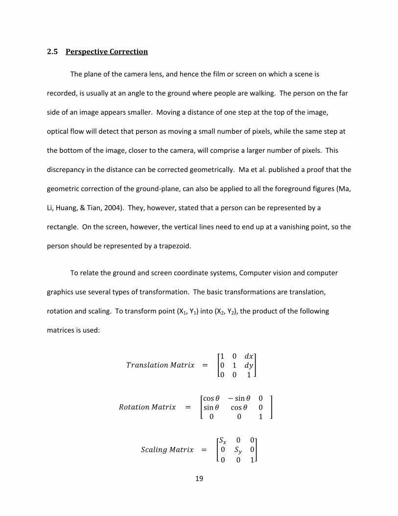
2.5 Perspective Correction ................................................................................................... 19

2.6 Vector Correlation .......................................................................................................... 20

3. PART 1: EXPERIMENTS USING CROWD VIDEOS ................................................................... 22

3.1 Methods ......................................................................................................................... 23

3.1.1 Manual Tracking .............................................................................................. 24

3.1.2 Optical Flow ..................................................................................................... 30

3.1.3 Alpha Equations ............................................................................................... 32

3.2 Results ............................................................................................................................ 38

3.2.1 Details of Varying Lukas-Kanade Optical Flow Parameters ............................. 39

3.2.2 Varying Manual Tracking Parameters ............................................................. 44

3.2.3 Varying Experiment Parameters ...................................................................... 51

vii

3.2.4 Lukas-Kanade Results vs PIV Results ............................................................... 62

3.3 Application: Using Alpha to Predict Trajectories .......................................................... 62

3.3.1 Using Alpha of Frames ..................................................................................... 62

3.3.2 Using Alpha Rows ............................................................................................ 64

3.3.3 Using Alpha of Cells ......................................................................................... 64

4. PART 2: EXPERIMENTS USING SIMULATION VIDEOS ........................................................... 68

4.1 Methods ......................................................................................................................... 68

4.1.1 Simulation Experiments ................................................................................... 69

4.1.2 Beta Approximation ......................................................................................... 76

4.1.3 Geometric Correction ...................................................................................... 77

4.2 Results ............................................................................................................................ 83

4.2.1 Transformation Matrix .................................................................................... 83

4.2.2 Results of the CP and PCI Processes ................................................................ 83

4.2.3 Other Results from the NetLogo Simulations .................................................. 88

4.3 Application: Using Beta to Predict Trajectories ............................................................. 92

5. DISCUSSION AND CONCLUSIONS .......................................................................................... 94

5.1 Sources of Error .............................................................................................................. 94

5.1.1 Stationary Background .................................................................................... 94

5.1.2 Shadow ............................................................................................................ 96

5.1.3 Color and Contrast ........................................................................................... 97

5.1.4 Geometry ......................................................................................................... 97

5.1.5 Direction of Motion, Crowd Density and Flow ................................................ 98

5.2 Conclusion ...................................................................................................................... 99

REFERENCES ............................................................................................................................. 104

viii

LIST OF FIGURES

Figure 1: Example of Optical Flow Vectors .................................................................................. 11

Figure 2: Graphs Comparing Simulation Outputs ........................................................................ 22

Figure 3: Process Flow Chart of Part 1 ......................................................................................... 24

Figure 4: Citrus Bowl Exit, Showing Manual Tracking Grid and Cell Numbers ............................ 25

Figure 5: Path of Individuals at the Citrus Bowl Exit Obtained Through Manual Tracking ......... 27

Figure 6: Velocity Vector Graph at the Citrus Bowl Exit Obtained Using Manual Tracking ........ 27

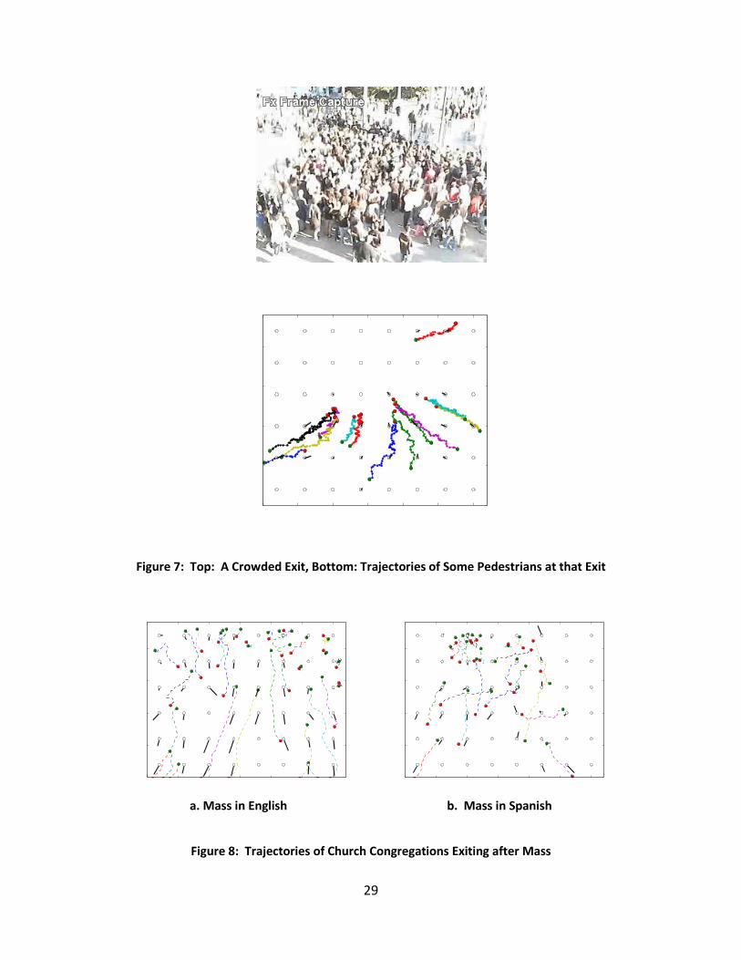
Figure 7: Top: A Crowded Exit, Bottom: Trajectories of Some Pedestrians at that Exit ............. 29

Figure 8: Trajectories of Church Congregations Exiting after Mass ............................................ 29

Figure 9: Average Number of People in Each of 48 Cells of 100 Frames Segment ..................... 35

Figure 10: Video Frame as It Appears After Using Various Thresholds ........................................ 41

Figure 11: Variation of Alpha of Frames with Aperture and Threshold ...................................... 42

Figure 12: Variation of Average of Alpha with Time at Various Thresholds (Clip S) ................... 42

Figure 13: Variation of Average of Alpha with Frames at Various Apertures (Clip S) ................. 44

Figure 14: Alpha Frame Calculated Using the Sum or Average of Manually Tracked Velocities 45

Figure 15: Alpha of Rows Using Vtot in a Sequence of ~1000 Frames .......................................... 46

Figure 16: Boxplot of Alpha Row Calculated Using Vtot ............................................................... 47

Figure 17: Number of People in a Row, in a Sequence of ~1000 Frames .................................... 47

Figure 18: Alpha of Rows Using Vave in a Sequence of ~1000 Frames ......................................... 48

Figure 19: Boxplot of Alpha Row Calculated Using Vave ............................................................... 48

Figure 20: Velocity of an Individual Is Spread from One Pixel (Red) to a Rectangle 10x25 ........ 49

Figure 21: Alpha Rows (L-K) after Spreading Manual Tracking Data ........................................... 51

Figure 22: Change of Alpha Frame and Its Coefficient of Variation with Cell Size ...................... 52

Figure 23: Vx of Optical Flow and Observed Trajectories, 20 X15 Cells, Single and Averaged Frames............................................................................................................................ 53

Figure 24: Alpha of Rows (using Vtot) vs. Number of People in the Row ..................................... 55

Figure 25: Average Coefficient of Variation of Alpha of Frames for Segments of Various Numbers of Averaged Frames ....................................................................................... 56

Figure 26: Frequency Distribution of Optical Flow Velocity Magnitude in a Set of 495 Frames . 57

Figure 27: Center Cells at the Exit ................................................................................................ 59

Figure 28: Alpha calculated from Sums of All Cells in the Frame and from Center Cells ............ 60

Figure 29: Vx of Center-Cells ........................................................................................................ 61

Figure 30: Vy of Center-Cells ........................................................................................................ 61

Figure 31: Alpha of Rows, LK and PIV........................................................................................... 62

Figure 32: Lukas-Kanade Optical Flow, Average Vectors (Red), One Frame (Black, Arrow Enhanced) ...................................................................................................................... 67

Figure 33: Flow Chart of the Process Used in Part 2 .................................................................... 68

Figure 34: Velocity of Turtles (Colored Arrows) .......................................................................... 71

Figure 35: NetLogo Set-Up Showing the 2-D Model View and the 3-D Perspective View .......... 72

Figure 36: Image of Cropped 320 x 240 Screen View Video Used as Input to Both Processes ... 73

ix

Figure 37: Image of Geometrically Corrected Video ................................................................... 74

Figure 38: Image of Geometrically Corrected Frame with PIV Vectors, a Step in the CP Process ....................................................................................................................................... 74

Figure 39: Cropped Video from Figure 36, after being processed by the PIV Optical Flow, an Intermediate Step in the PCI Process ............................................................................ 75

Figure 40: Velocity Positions ........................................................................................................ 76

Figure 41: Change of Ground Coordinates to Model Coordinates .............................................. 78

Figure 42: Perspective and Screen images, transformed to Model Image ................................. 79

Figure 43: Average Optical Flow .................................................................................................. 84

Figure 44: Vy of Average of 20 frames; NetLogo Tracks, CP-PIV and PCI-PIV .............................. 85

Figure 45: Histogram of Vy from NetLogo Tracks and PIV, Data from All Cells in 20 Frames ...... 86

Figure 46: Histograms of Vy from the CP and PCI Processes, Data from All Cells in 20 Frames .. 86

Figure 47: Pareto Chart of the CP (Top) and PCI (Bottom) Processes ......................................... 90

Figure 48: Contour Plot of the Correlation, With Generation Rate and Turtle Size as Axes ....... 91

Figure 49: Contour Plot of the Correlation, With Step and Turtle Size as Axes .......................... 91

Figure 50: Contour Plot of the Correlation, With Generation Rate and Step as Axes ................. 92

Figure 51: PIV Optical Flow Vectors of Turtles Moving on a Gridded Background ..................... 95

Figure 52: PIV Optical Flow Vectors of Turtles Moving on a Plain Background .......................... 95

Figure 53: Temporal Average of Video at Citrus Bowl Exit .......................................................... 96

Figure 54: Citrus Bowl Exit Image after Geometric Transformation ........................................... 98

x

LIST OF TABLES

Table 1: Coefficient of Variation of Alpha Frame (using Vtot,clip S) ............................................. 40

Table 2: Coefficient of Variation of Alpha Averaged over 50, 100 and 200 Frames ................... 55

Table 3: Alpha of Center Cells ...................................................................................................... 59

Table 4: Correlation between Predicted and Actual Velocities ................................................... 63

Table 5: Vector Correlations between Observed and Predicted Velocities in the 8x6 Cells ....... 65

Table 6: Relative Error between Observed and Predicted Tracks using Alpha-Cell .................... 66

Table 7: Vector Correlations of Velocities between NL data and Processed Data ...................... 87

1

1. INTRODUCTION

When I started to work as a graduate research assistant with the SimMBioS Project at

the Institute for Simulation and Training of the University of Central Florida, there were several

simulation models under investigation. There was a crucial requirement to find a quantitative

relation between the simulations and real crowd movement, which can tell us whether a

simulation is representative of real crowds or not, and which of a number of simulations

models real crowds better. This is where my research was positioned. The simplest simulation

consists of a room with an exit. A number of circles representing people are in the room at the

beginning. The people are programmed to move according to some model. The circles try to

exit from the room. I started comparing crowd simulation data output that were based on the

Helbing and Flocking models. Each model has parameters that can be varied, and this affects

how simulated people exit the room. However, how do we know which model and which

parameter represents the behavior of real people? If we have videos of a real crowd exiting a

room, we want to compare the video to the simulation to find out which simulation is “better”.

There has to be a way to measure what we mean by “a better simulation”. This work is a

contribution towards that goal.

1.1 Definitions

Crowds are around us everywhere. We see crowds at airports, in sports arenas, at

festivals, and at many entrances and exits. Crowds considered in this research are pedestrian

2

crowds; similar research can be applied to vehicular traffic. Merriam Webster Dictionary has

several definitions for the word “crowd”, the one that is considered here is: “a large number of

persons especially when collected together” ("crowd," 2009). A more precise definition is “a

collection of pedestrians occupying a common area and with varying degrees of interaction

with each other (Leggett, 2004)”. Only crowds that are moving in a somewhat specific direction

are investigated here.

Videos of crowds consist of consecutive images, called frames. Each frame consists of

an array of pixels, for example 320 x 240, each with an intensity (or gray level). A color image

consists of three sets of 256-gray-level images, one for each of the colors red, green and blue

(RGB). To extract information from a crowd video, it goes though some image-processing

software, and then the results can go through an image-understanding algorithm, which

differentiates, for example, foreground from background, or pedestrian from tree. The aim of

processing video images is to detect the motion of pedestrians in each image. Comparing

locations in consecutive frames gives an indication of the motion of the pedestrians. Optical

flow is the automatic estimation of the apparent movement of these shapes from a sequence

of images. Its result is a matrix of velocity vectors that describes the motion direction and

intensity in different areas in the frame.

The expression “Crowd Flow” paints a picture of a river of people. This is the type of

crowd movement studied here. Crowd movement has a speed and a direction. Many times

crowd density is also a factor in analyzing crowd movement. Studying the “flow” of a crowd is

performed by looking at the crowd from a macroscopic level. There is also research performed

3

on a microscopic level. The latter involves tracking individual people within the crowd. Both

points of view can be looked at by using optical flow, and both types of motion can be studied

using simulations. There is also a finer level of software that tracks the limbs of individuals or

even facial expressions (Teknomo, Takeyama, & Inamura, 2001); (Hoogendoorn, Daamen, &

Bovy, 2004);(Hu, Tan, Wang, & Maybank, 2004).

Crowd simulations, as considered in this work, are computer programs that represent

the real crowds. Some represent the flow of pedestrians as a whole, just like the flow of a fluid

represents the motion of all molecules in it. Simulations can also be constructed by modeling

the behavior of individual persons: where they decide to go and how they get there. Another

type that also falls under the umbrella of simulations is more detailed, such as modeling

gestures and facial expressions. This type is outside the realm of the study of “crowds”.

Users of simulations base their decisions on the results that are output by these

simulations. Therefore, one must be confident that these results are valid. For that reason,

computer programs, in general, have to be verified and validated. Verification is defined as

ensuring that the model implemented is correctly written in the software program. Validation

means that the program, as written, properly represents the process that it is supposed to

model, within an acceptable range of accuracy (Sargent, 2008). The SimMBioS project

endeavors to construct simulations that model real crowds. Thus there is a need to find a way

to verify and validate the simulations and that their generated data do model that of a given

crowd.

4

1.2 Motivation

Validation of the results of a crowd simulation is an important step to ascertain that the

right model has been built to represent real pedestrian crowd behaviors. There are several

mathematical models available for simulating crowds (Reynolds, 1987). And each of these

models has parameters that can be varied. Comparing their results will generally show that the

generated output data, for example how fast people exit a room, have different values. Which

output, hence what parameter setting in a given simulation model, represents real life better?

The model must be compared to the actual situation that it represents, and the parameter

values used in the simulation should be chosen so as to correspond to the real system.

The question arises as to how to validate these various simulations with their range of

parameters. How do we determine that the simulation represents the real situation? One

method is to have subject matter experts “look” at the animation of the simulation and at the

video of the crowd and determine that they behave alike. The effectiveness of this kind of

correspondence is not quantitatively measurable. Another method may involve manually

tracking individuals in the crowd video comparing their aggregate behaviors with the

aggregation of the simulation. This method is too time-consuming to be useful extensively.

Hence, it would be of benefit to have an analysis of the crowd video and the simulation

performed automatically using software. This could save time and money in the process of

validating a simulation, and is expected to have a quantifiable accuracy.

Having software read video which could then generate and output the values of certain

crowd parameters is feasible but needs to be validated. To this end, this research is attempting

5

to validate results from software, generally performing optical flow analysis. The objective of

the study in this thesis is to understand the factors that affect optical flow, using various

experiments, in order to find a quantitative measure to compare output from the optical flow

software to results obtained by manually tracking individual persons in crowd videos (or tracks

from simulations). This is to assess the quality and adequacy of these methods. The aim is to

find a reliable quantitative method to validate and calibrate the results of the optical flow

analysis, so that optical flow can in turn, be used to validate crowd simulations.

1.3 Challenges

Reliable output data is needed from the optical flow software in a form that can be used

to validate crowd simulations. Optical flow is sensitive to any changes in the environment, not

only moving individuals; and real situations will generally have moving shadows, swaying tree

branches, waving flags etc. Some researchers stage indoor crowds for their studies. This thesis

uses videos of real crowds or data from simulations, compares them to tracked paths, and

attempts to measure their correspondence.

Ordinarily, computer-based methods that attempt to identify individuals in crowds

encounter difficulties when there are larger crowds. Occlusion, one person being hidden from

the view of the camera behind another person or object, could result in errors. Two people

walking in opposite directions but in the same line of view of the camera, may be seen as one

blob, so do people that are touching. Sparse crowds also create difficulties, as they do not

result in a continuous flow. Lighting changes can also be deceiving. Errors arising from a door

6

opening and closing as in a train station, from the shadow of tree branches blowing in the wind,

and even from the shadow of a person walking near a light pole, are challenging to eliminate.

Video format is also a key factor. Treating a video as three layers of colors gives

different results from black and white treatment. Different compression methods of digital

videos affect how they are read by optical flow software. MPEG and MPEG-4 cause loss of

high-frequency information and should be avoided. A more detailed description of challenges

in video analytics can be found in (Gagvani, 2009).

1.4 Scope

There are various levels of optical flow analysis. On the fine side, software may be

needed to identify individuals, for example to count passengers in a transit station, as numbers

may vary by time of day, day of week and season. This type of accuracy is not considered in this

work. Similarly, fine results are needed for some types of surveillance. Methods to identify and

track a specific person in a crowd are being developed (Mahalingam, Kambhamettu, & Aguirre,

2009) and were surveyed (Moeslund, Hilton, & Krüger, 2006). Additionally, work on identifying

facial characteristics, walking gait, and people’s gestures is described in Hu et al. (2004). These

uses are not included in this work.

The videos studied here come from one stationary camera. Some research requires

using optical flow to identify three-dimensional shapes. This type is necessary in robotics for

tracking moving objects (Inoue, Tachikawa, & Inaba, 1992), and also in medicine for researching

7

tumors (Guerrero, Zhang, Huang, & Lin, 2004). To a great extent, that research requires the use

of more than one camera. This category is also not included here.

This thesis is concerned with a relatively coarse analysis. The optical flow software used

is not intended to detect individuals, even though at some levels it could. Crowd motion is

visualized as closer to a flow. The behavior of individuals is not studied, rather that of the

group as a whole. Comparisons of optical flow and manual tracking of the individuals in the

crowds are used to calibrate how the average individual velocities can be established from an

optical flow. Some information on individuals’ behaviors can come as a side-result from

observed trajectories of individuals in crowd videos, such as speed distribution of individuals in

the crowd or insights into how family units walk together.

1.5 Outline

The next chapter gives some more detailed background information. Published

research that describes a number of methods used in this thesis is cited. In addition, reference

is made to papers that survey, in more detail, the area of crowd analysis.

Chapters ‎3 and ‎4 describe the work done in Part 1 and Part 2 of the research. Each

begins by reporting the methods used, including definitions and equations. This is followed by

the results. Chapter ‎3 details the mathematics behind an assumed isotropic proportionality

calibration constant alpha. The results of this method (the alpha method) at relating optical

flow of real crowd videos to observed tracks are shown, including the effect of varying optical

flow parameters, averaging manually tracked data and effects of various experimental

8

conditions. Chapter ‎4 describes results of using optical flow of simulations and comparing them

to actual tracks. A new method beta, which relates the velocity vectors by a different

approximation, is shown. The two methods are detailed and their results outlined.

Chapter ‎5 concludes the thesis. It discusses a number of sources of error. A summary

of results is given, with some suggestions for future research.

9

2. BACKGROUND

2.1 Manual Tracking of Individuals in a Crowd

A variety of factors influence the movement of a pedestrian crowd. “… age, gender,

physical fitness, social relationship to neighboring pedestrians, purpose of journey …” (Velastin

et al., 1994). Density, culture and panic level are also factors. Manual tracking by an human

observer of individuals in a video, is performed to detect how people behave in which

situations (B. Zhan, Remagnino, Monekosso, & Velastin, 2009). Some algorithms require that a

spatial region of interest be manually specified at the beginning of the analysis (Mahalingam, et

al., 2009). In some cases, where a software needs training to recognize human figures, initially

human figures are detected manually (Dalal, Triggs, & Schmid, 2006).

Teknomo et al. in 2000 collected data manually to obtain pedestrian movement

variables. They converted a video into a stack of 150 images, with one frame taken every 0.5

seconds. A cross-hair placed at the head of every individual depicts the x-y position in every

frame. They state that a single person can collect about 40-60 pedestrian paths in eight hours.

The output has a person id number, frame number, and position coordinates x and y. The data

was then trimmed to the area that they wanted to investigate, and only the pedestrians passing

through that area were examined. They converted the image coordinates to real world

coordinates using linear regression, and then they graphed the head-path movement of the

pedestrians. They found that the path of pedestrians included a sideways motion (due to their

gait) superimposed on the forward motion in the direction in which they were headed. For

10

each individual in the video, they calculated an instantaneous speed, a time mean speed (sum

of speeds divided by number of observations), average speed (total walking distance divided by

time). They also obtained density (number present in investigation area / area). Flow, the

average number of persons crossing a given line in a given interval of time, was also

determined. Due to the sideways motion, the instantaneous velocity was oscillating, and they

found it best to use a moving average over a large time interval to smooth the graph (Teknomo,

Takeyama, & Inamura, 2000).

2.2 Optical Flow

There is a wide range of literature that describes specific mathematical and statistical

calculations or software to extract detailed information from optical flow, also called optic flow.

References dealing with optical flow, which is used to extract information from images that are

not dealing with crowds and pedestrians, can be found in a survey by Rokia and Roman (2005).

This section only surveys the basic methods to extract information from videos of crowds.

Survey papers are listed below for a more detailed treatment.

“Optical flow is the distribution of apparent velocities of movement of brightness

patterns in an image” (Horn & Schunck, 1980). Visually, optical flow is a vector field that shows

the direction and magnitude of these intensity changes from one frame to the next, as

illustrated in Figure 1. It does not give us the three-dimensional movement of an object since a

video is only 2D. Thus only the projection of this movement onto the two-dimensional image is

obtained. The process by which an optical flow is calculated is based on the hypothesis that the

intensity and spatial structure of a local image remains constant under motion for a very short

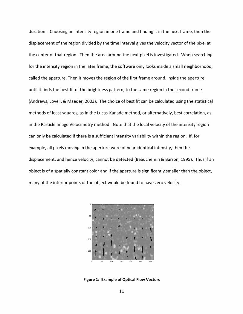
11

duration. Choosing an intensity region in one frame and finding it in the next frame, then the

displacement of the region divided by the time interval gives the velocity vector of the pixel at

the center of that region. Then the area around the next pixel is investigated. When searching

for the intensity region in the later frame, the software only looks inside a small neighborhood,

called the aperture. Then it moves the region of the first frame around, inside the aperture,

until it finds the best fit of the brightness pattern, to the same region in the second frame

(Andrews, Lovell, & Maeder, 2003). The choice of best fit can be calculated using the statistical

methods of least squares, as in the Lucas-Kanade method, or alternatively, best correlation, as

in the Particle Image Velocimetry method. Note that the local velocity of the intensity region

can only be calculated if there is a sufficient intensity variability within the region. If, for

example, all pixels moving in the aperture were of near identical intensity, then the

displacement, and hence velocity, cannot be detected (Beauchemin & Barron, 1995). Thus if an

object is of a spatially constant color and if the aperture is significantly smaller than the object,

many of the interior points of the object would be found to have zero velocity.

Figure 1: Example of Optical Flow Vectors

12

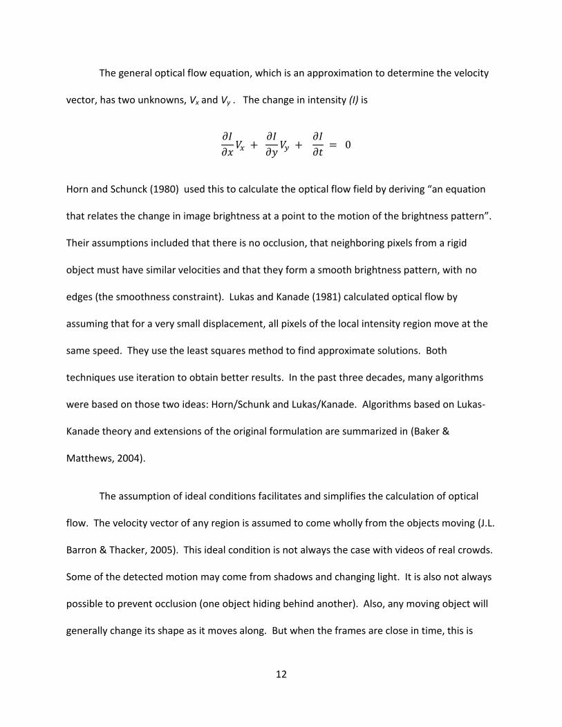
The general optical flow equation, which is an approximation to determine the velocity

vector, has two unknowns, Vx and Vy . The change in intensity (I) is

Horn and Schunck (1980) used this to calculate the optical flow field by deriving “an equation

that relates the change in image brightness at a point to the motion of the brightness pattern”.

Their assumptions included that there is no occlusion, that neighboring pixels from a rigid

object must have similar velocities and that they form a smooth brightness pattern, with no

edges (the smoothness constraint). Lukas and Kanade (1981) calculated optical flow by

assuming that for a very small displacement, all pixels of the local intensity region move at the

same speed. They use the least squares method to find approximate solutions. Both

techniques use iteration to obtain better results. In the past three decades, many algorithms

were based on those two ideas: Horn/Schunk and Lukas/Kanade. Algorithms based on Lukas-

Kanade theory and extensions of the original formulation are summarized in (Baker &

Matthews, 2004).

The assumption of ideal conditions facilitates and simplifies the calculation of optical

flow. The velocity vector of any region is assumed to come wholly from the objects moving (J.L.

Barron & Thacker, 2005). This ideal condition is not always the case with videos of real crowds.

Some of the detected motion may come from shadows and changing light. It is also not always

possible to prevent occlusion (one object hiding behind another). Also, any moving object will

generally change its shape as it moves along. But when the frames are close in time, this is

13

likely to be a lesser problem. However, quantitative estimates of how bad this could be are still

to be given.

Various algorithms to compute optical flow differ in their performance and the

computing power required. Galvin et al. evaluated eight optical flow algorithms (1998). They

did so by comparing them to ground-truth motion fields of scenes of arbitrary complexity. The

study found that “a modified version of Lucas and Kanade’s algorithm has superior

performance but produces sparse flow maps”. They also found that the second best was an

algorithm by Proesmans et al. provided reasonable results, and produced a flow vector for each

pixel.

Particle Image Velocimetry (PIV) originated as an optical method to visualize the

movement in a fluid. A homogeneous fluid does not reflect or scatter visible light. Particles can

be dispersed in the fluid in such a way that the particle displacements represent the flow of the

liquid. The displacement could be measured from double exposed photographs or from two

images taken within a short time interval, and thus give information on the flow of the fluid.

Even though the individual particles cannot be identified, the displacement of the region of

particles under investigation is an indication of the average of the local velocity of the fluid

(Westerweel, 1997). This same idea is adaptable to study the flowing motion of crowds. The

optical flow is found using cross-correlation between the consecutive frames. PIV can work

using color images. It can compare large areas and does not need to use small cells (Quénot,

Pakleza, & Kowalewski, 1998), in contrast to the Lukas-Kanade method, where the largest

aperture is 15x15 pixels. The PIV software used in this work was adapted by Dr. Thomas Clarke.

14

It is difficult to create a universal algorithm to analyze real word data using optical

flow, as each setting has a different layout and positioning of the camera. The degree of

distortion arising from the location and camera position will not only be unique for every

situation, but it will also distort the shapes of pedestrians, or vehicles, in a non-uniform way

depending on their position in the frame. For example, the image of a person will seem larger

when he or she is closer to the camera. The shapes of moving objects can change over a

sequence of frames, such as a turning car. People are also not rigid. They change shape as they

move their arms and legs. Lighting plays tricks with colors as with the shades of gray in black

and white images. A change in the shade of gray may be caused by a passing cloud, not by

movement. Light also creates reflection and shadows, which may appear to be moving objects.

Moving objects can be partially concealed by other objects (occlusion). Some algorithms are

built on predicting the next move of an object. People, however, are highly unpredictable

(Vicencio-Silva, 1994).

Optical flow analysis is useful in fields other than human motion capture. It can be used

to analyze the motion of the heart wall and blood flow in medical imaging or in the diagnosis of

orthopedic patients (Moeslund & Granum, 2001). In sports it can be used to investigate an

athlete’s performance (Moeslund, et al., 2006). In agricultural research, it was used to measure

minute growth in seedlings (Beauchemin & Barron, 1995).

2.3 Verification and Validation of Crowd Simulations Using Optical Flow

After building a simulation, there must be a method to judge whether or not it

accomplishes what it is expected to do. Malone et al. (2008), also (Malone, Clarke, Oleson II,

15

Rosa, & Faulkner, 2007), attempted to find a quantitative method to compare crowd data to

simulations. They showed that optical flow can depict the motion pattern from videos.

However, optical flow needs to be calibrated in order to be used to validate simulations. Clarke

et al. (2007) showed that when optical flow from a video is averaged within a boundary, and

compared to the flux of people crossing the edges of the same boundary, then there is a linear

relationship observed. Kaup et al. (2008) showed that the optical flow fields of videos, taken at

a church exit, can differentiate between the directional motion of the Anglo congregation and

the mulling around motion of the Hispanic congregation.

2.4 Crowd Movement Detection

The movement of pedestrian crowds can be studied on both the macroscopic and the

microscopic levels. In macroscopic studies, density, average speed and direction of the flow are

involved. On the microscopic scale, the characteristics of individuals are examined. These

include preferred speed, and interaction with surroundings. Interactions affect the distances

kept between individuals and the behavior of groups walking together.

Hu et al. (2004) divided the process of detection and tracking of crowds into stages. First

the environment may be modeled. This is sometimes used to separate the background from

foreground, assuming the foreground pixels represent the moving people. The background is

found by temporal averaging or other estimation methods, including using filters. Another

method is to compare two image frames pixel by pixel. If the colors are the same, replace the

pixel with the color white, else, keep the new pixel. The second step is to detect moving

objects by segmenting these regions from the background. One of the methods is to use

16

optical flow vectors to detect the movement. In a further stage, the moving regions may be

classified according to their shape or their motion. They could be, for example, people,

vehicles, birds, clouds. Further analysis can lead to tracking moving objects from frame to

frame, by matching, for surveillance purposes. This can be achieved by tracking image regions,

or by using outlines as contours and updating these contours, or by extracting parts of the

image and clustering them into higher level features, then matching features between images.

The tracked shapes can be matched to pre-prepared models, such as human body, vehicle, or

human limbs and joints. There are a variety of methods to search for the comparable models

utilizing statistics. If individual humans can be tracked, their behavior can then be studied as

features that can be classified by how they vary in time (Hu, et al., 2004).

Some backgrounds are not stationary. These cannot be directly subtracted from the

image. The moving parts of those backgrounds are not the crowds we are trying to detect.

They can be tree branches swaying or a flag fluttering in the wind, also waves, smoke or fire.

These motions have patterns. Methods to recognize them using optical flow are described by

Fazekas and Chetverikov (2005).

2.4.1 Detecting Abnormal Motion

Detection of abnormal events and disturbances in crowds present in public places is a

different type of crowd motion detection. It is required in surveillance situations. This is

valuable information for maintaining security in public assemblies and sports events, as well as

in demonstrations, strikes and protests. Surveillance may be on a very fine level, if the aim is to

track one person in a crowd. A coarser level is also useful. In this case one is looking for a

17

crowd element with nonconforming behavior among the rest of the crowd. If someone falls

down at an arena exit, people would walk around that area. Or if there is a fight among

demonstrators, optical flow can point out that region. Andrade et al. collect optical flow

information of normal scenes. By comparing a situation to the learned “normal” optical flow,

they can detect anomalies (Andrade, Blunsden, & Fisher, 2005, 2006; Andrade, Fisher, &

Blunsden, 2006). Davies et al. detected likely crowd congestion as people stop. They did that

by detecting that the up-and-down oscillatory movement of the heads of walking people has

stopped. This was an indication of congestion (Davies, Jia Hong, & Velastin, 1995).

2.4.2 Density and People Counting

There are essentially two techniques to estimate crowd density using optical flow. One

technique is based on foreground pixel counting, and the other is feature-based. Pixel counting

methods require background segmentation first, to leave the foreground that consists mainly of

moving people (Lo & Velastin, 2001). A human can look at a surveillance video of crowds

moving and identify a person from a car, a column from a gate, a small group from a crowd,

walking from running. This process is much more complicated for a computer. Software needs

to process the images to organize a group of pixels into categories that can be processed

further and compared to stored templates or categories. Various sciences, such as computer

vision and animation, are involved in this procedure. These indexed categories can then be

used to identify objects in new scenes.

People in an image could be counted by analyzing the area of moving pixels. Using

segmentation of the foreground pixels, assuming that they represent moving non-rigid bodies,

18

and under various environmental conditions, Zhang & Sexton were able to count people in a

crowd with an error of 17% in their counts (1995). Chen and Hsu used an overhead camera and

an estimate of people sizes; a rough count was performed, then refined using histograms of

intensity and color hue (Chen & Hsu, 2003). The size of people changes depending on their

location in the picture. Park et al. (2006) corrected for that. They divided their region of

interest into 72 cells and assumed the shape of a person to be a rectangle. They then

calculated the size of a person in each cell using projections, and used this estimate in counting

people (Park, et al., 2006).

2.4.3 Survey Papers

Motion-based recognition, not necessarily using optical flow, is surveyed by Cédras and

Shah (1995). Beauchemin reviewed the computation of optical flow, including the problems

encountered (Beauchemin & Barron, 1995). Gavrila analyzed the literature on motion

detection of the whole body or the hand. He divided the methods into 2-D without models

(low level, using statistical descriptions to detect a body) and with models (detecting body

parts), and also 3-D methods (Gavrila, 1999).

Zhan et al. (2008) surveyed crowd analysis. They included methods of density

estimation, face recognition, crowd recognition and tracking a person in the crowd. They also

discussed crowd modeling that is based on recurring behavior and is used in further analyzing

video data. They ended with discussing crowd analysis methods that are not based on

computer vision analysis (Beibei Zhan, et al., 2008).

19

2.5 Perspective Correction

The plane of the camera lens, and hence the film or screen on which a scene is

recorded, is usually at an angle to the ground where people are walking. The person on the far

side of an image appears smaller. Moving a distance of one step at the top of the image,

optical flow will detect that person as moving a small number of pixels, while the same step at

the bottom of the image, closer to the camera, will comprise a larger number of pixels. This

discrepancy in the distance can be corrected geometrically. Ma et al. published a proof that the

geometric correction of the ground-plane, can also be applied to all the foreground figures (Ma,

Li, Huang, & Tian, 2004). They, however, stated that a person can be represented by a

rectangle. On the screen, however, the vertical lines need to end up at a vanishing point, so the

person should be represented by a trapezoid.

To relate the ground and screen coordinate systems, Computer vision and computer

graphics use several types of transformation. The basic transformations are translation,

rotation and scaling. To transform point (X1, Y1) into (X2, Y2), the product of the following

matrices is used:

20

The perspective transformation from a camera screen to ground coordinates is more

involved. The transformation matrix requires knowledge of the focal length of the camera lens,

as well as the exact position of the camera relative to the image, in order to calculate the

camera rotation and its displacement translation (Shah, 1997). This information is usually not

available when one acquires a video. However, that can be bypassed if the positions on the

ground are known. The perspective transformation matrix used in this thesis was obtained by

comparing the positions of specific points on the screen to their corresponding points on the

ground and using least squares to obtain the best matrix that minimizes the error between the

two (Clarke, 2009).

2.6 Vector Correlation

Velocities are vectors that have magnitudes and directions, and can be represented by

their components and . There are several methods to find correlation between two

vectors, and their results are not identical. One technique is to use the angular error between

two optical flow vectors as a measure of performance (J. L. Barron, Fleet, Beauchemin, &

Burkitt, 1992). The method we finally used here to compare vectors was described by Hanson

(1992). He uses complex numbers for vectors z and w.

where and are the components of vector , and so forth.

The variance and covariance for N vectors are

21

( 1 )

and

( 2 )

Hanson then defines a vector correlation measure as:

( 3 )

is a complex number. The real portion is essentially a dot-product which measures

how well the magnitudes of the z’s and w’s align and is the sum of the covariance between

corresponding elements of the variables, while the imaginary part is essentially a cross-product

of the z’s and w’s and measures how well the directions of the z’s and w’s align. A value of the

real part of close to 1 implies higher correlation in the amplitudes, while 0 implies no

correlation. When the value of the imaginary part of is near zero, the directions are

strongly aligned.

22

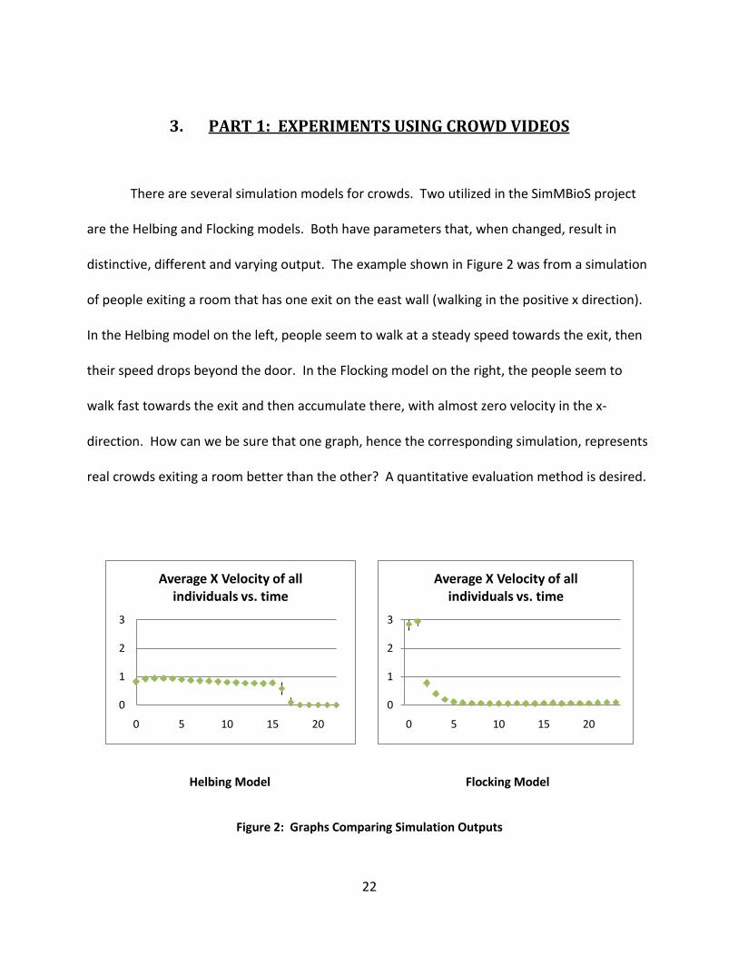
3. PART 1: EXPERIMENTS USING CROWD VIDEOS

There are several simulation models for crowds. Two utilized in the SimMBioS project

are the Helbing and Flocking models. Both have parameters that, when changed, result in

distinctive, different and varying output. The example shown in Figure 2 was from a simulation

of people exiting a room that has one exit on the east wall (walking in the positive x direction).

In the Helbing model on the left, people seem to walk at a steady speed towards the exit, then

their speed drops beyond the door. In the Flocking model on the right, the people seem to

walk fast towards the exit and then accumulate there, with almost zero velocity in the x-

direction. How can we be sure that one graph, hence the corresponding simulation, represents

real crowds exiting a room better than the other? A quantitative evaluation method is desired.

Helbing Model Flocking Model

Figure 2: Graphs Comparing Simulation Outputs

0

1

2

3

0 5 10 15 20

Average X Velocity of all individuals vs. time

0

1

2

3

0 5 10 15 20

Average X Velocity of all individuals vs. time

23

To compare the simulations to real crowd videos, optical flow was used to estimate

crowd velocity from the videos. I will describe various experiments in this part which were

carried out to calibrate an optical flow calibration constant, herein called alpha. Two methods

of optical flow were used, Lukas-Kanade and Particle Image Velocimetry (PIV). The aim of the

research was to understand the capabilities and limitations of using optical flow from videos of

real crowds, and how to calibrate the results to compare them with manually observed tracks.

Factors examined included aperture and threshold used in the optical flow software, as well as

determining the effect of cell size and number of frames averaged.

3.1 Methods

Ideal conditions are always sought. Some researchers use actors to create videos of

crowd flow. They refine their experiment of staged crowd movement by asking their

participants to walk “naturally”. There is no general way to validate that the actors were

walking “naturally”. This work herein starts by analyzing videos of people exiting an actual

sports arena and a church, where the people were unaware of the video and were truly walking

“naturally”. Concentration was on a video of an exit at the Citrus Bowl sports arena.

The processes in Part 1 of the thesis are charted in Figure 3. A video was chosen and

visually assessed. It was run through a manual tracking software, where a person actually

marks on a video frame each pedestrian appearing on the screen, and follows the position of

the person from frame to the next (or every 5 frames). The video was also processed through

two optical flow programs, one based on the OpenCV and Lucas-Kanade (LK) method, the other

on the Particle Image Velocimetry (PIV) method. The resulting data were compiled and

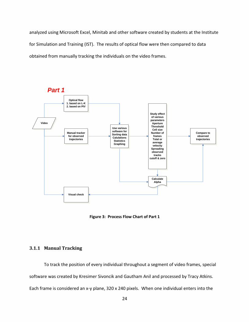
24

analyzed using Microsoft Excel, Minitab and other software created by students at the Institute

for Simulation and Training (IST). The results of optical flow were then compared to data

obtained from manually tracking the individuals on the video frames.

Optical flow

1. based on L-K

2. based on PIV

Video

Visual check

Calculate

Alpha

Compare to

observed

trajectories

Manual tracker

for observed

trajectories

Study effect

of various

parameters

Aperture

Threshold

Cell size

Number of

frames

Total or

average

velocity

Spreading

observed

tracks

cutoff & zero

Use various

software for

Sorting data

Calulations

Statistics

Graphing

Part 1

Figure 3: Process Flow Chart of Part 1

3.1.1 Manual Tracking

To track the position of every individual throughout a segment of video frames, special

software was created by Kresimer Sivoncik and Gautham Anil and processed by Tracy Atkins.

Each frame is considered an x-y plane, 320 x 240 pixels. When one individual enters into the

25

scene, a crosshair marker is placed on the head, which specifies the x-y position in the frame.

This marker is moved to the new position corresponding to the location of the head of that

individual after every five-frame interval. It is important to note that tracking the head of

individual using manual tracking software implies that the person’s velocity may be accounted

for in one cell, while actually the rest of his body may be moving in a different cell.

The videos used were 320 x 240 pixels and were shot at a rate of 25 or 30 frames per

second. A frame can be divided into cells, where the velocities of the heads of individuals in the

cell can be summed up or averaged. Figure 4 shows a frame, and an overlaid grid with 8×6

numbered divisions (cells); each cell is 40x40 pixels. Other cell sizes were also investigated.

Smaller cells gave poorer fit with larger coefficient of variation of alpha; conversely larger cells

gave lower variation in exchange for lower spatial resolution.

Figure 4: Citrus Bowl Exit, Showing Manual Tracking Grid and Cell Numbers

26

The output of the program used in the SimMBioS project consisted of an xml file with

every tracked person’s id number and his x-y location in every fifth frame. Data from this xml

file was fed to other software to calculate statistics. For the purposes of this work, the frame

was divided into cells and the total velocity (sum of individual velocities) of all the individuals in

a cell was summed up. The velocities were only counted in those cells where the crosshair (on

the head) was located. The data collected this way does not account for the motion of the rest

of the body, which could be in a different cell. Note that, on the other hand, the optical flow,

counts that motion in the different cell. The output of the Manual Tracking program consisted

of the frame number, cell number (or coordinates of cell), also Vx and Vy, the components of

the total velocity of the individuals whose heads are in a cell. The output also included the

number of people (actually their heads) in the cell and the components of the average velocity

so counted in that cell. Statistical software can then be used to extract useful information from

the data.

Results of manual tracking of individuals’ paths can be displayed in several ways. One

form is to display the tracks of individuals over some frames, as shown in Figure 5. This plot can

be used to visually validate the results of the manually tracked trajectories. The location of

every individual in all the frames can be translated into individual velocities of pixels per frame.

From this the velocity distribution of the group can be found.

Another form of output is a vector field representing the average or total velocity of

individuals in each cell. This is actually either the sum of all velocities of pixels in the cell that

have a velocity associated with them, or the average obtained by dividing this total velocity by

27

the number of individuals (really their heads) moving in that cell. An example of this vector

graph is shown in Figure 6. This graph can be used to compare to optical flow results.

Figure 5: Path of Individuals at the Citrus Bowl Exit Obtained Through Manual Tracking

Figure 6: Velocity Vector Graph at the Citrus Bowl Exit Obtained Using Manual Tracking

There are other observations that can be concluded from looking at graphs of

trajectories, which confirm results of previous research. Figure 5 shows how people’s heads are

bobbing left and right, and how they do not walk in a straight line, though the bulk of their body

28

may appear to be moving forward. The path a person takes is especially crooked when it is

crowded, as the plot of paths at the exit in Figure 7 shows. People are trying to locate an

available spot to walk among the crowd. The crooked paths also show that manually obtained

trajectories by tracking the heads of pedestrians could use some smoothing before using the

data to compare to optical flow data.

Figure 5 can also be used in building the simulation. The paths that individuals walk

show whether people usually walk in a lane, behind - or across the paths of - other individuals,

and where they are coming from and going to. Knowing the layout of the arena, one can also

learn whether individuals exit from the same side they are parked on, or they come out from

one side and cross the gate to the other towards their parking. Closer observation of the video

and correlation with manual trajectory results that include identifying a person by unique id

numbers can also lead to tracking certain individuals that form a group, for example a family, to

observe their preferred speed and distance from each other, information always welcome to

build and validate simulations.

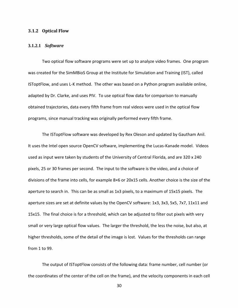
One other result obtained from manual trajectory tracking was observing different

behaviors. The exit of a church was videotaped after mass performed in English and after

another performed in Spanish. The results of paths of the exiting congregations are shown in

Figure 8. They show that people leaving after the English mass seem to walk straight out, while

people leaving after the Spanish mass tend to mill around, possibly socialize.

29

Figure 7: Top: A Crowded Exit, Bottom: Trajectories of Some Pedestrians at that Exit

a. Mass in English b. Mass in Spanish

Figure 8: Trajectories of Church Congregations Exiting after Mass

30

3.1.2 Optical Flow

3.1.2.1 Software

Two optical flow software programs were set up to analyze video frames. One program

was created for the SimMBioS Group at the Institute for Simulation and Training (IST), called

ISToptFlow, and uses L-K method. The other was based on a Python program available online,

adapted by Dr. Clarke, and uses PIV. To use optical flow data for comparison to manually

obtained trajectories, data every fifth frame from real videos were used in the optical flow

programs, since manual tracking was originally performed every fifth frame.

The ISToptFlow software was developed by Rex Oleson and updated by Gautham Anil.

It uses the Intel open source OpenCV software, implementing the Lucas-Kanade model. Videos

used as input were taken by students of the University of Central Florida, and are 320 x 240

pixels, 25 or 30 frames per second. The input to the software is the video, and a choice of

divisions of the frame into cells, for example 8×6 or 20x15 cells. Another choice is the size of the

aperture to search in. This can be as small as 1x3 pixels, to a maximum of 15x15 pixels. The

aperture sizes are set at definite values by the OpenCV software: 1x3, 3x3, 5x5, 7x7, 11x11 and

15x15. The final choice is for a threshold, which can be adjusted to filter out pixels with very

small or very large optical flow values. The larger the threshold, the less the noise, but also, at

higher thresholds, some of the detail of the image is lost. Values for the thresholds can range

from 1 to 99.

The output of ISToptFlow consists of the following data: frame number, cell number (or

the coordinates of the center of the cell on the frame), and the velocity components in each cell

31

Vx and Vy This is the average of the velocities of all pixels in a cell, including those where no

motion was detected. If we have 8×6 cells, this means that 40x40 = 1600 pixels are averaged in

each cell, and we have a coarse image of how the velocity vectors look in the cell. If we choose

320 x 240 cells, we are at the 1x1 pixel level, and we have the finest detail, a velocity vector for

every pixel.

The PIV software was based on a Python program available online (Gurka & Liberzon,

2007), and modified by Dr. Thomas Clarke. It analyzes a video using a choice for data spacing

(similar to cells, it determines where the velocity vector is going to be placed) and investigation

window (similar to apertures). Output is similar to the ISToptFlow software, with Vx and Vy

components in every cell in every frame.

3.1.2.2 Relating Optical Flow to Observed Velocities: Alpha Approximation

Alpha ( was chosen to represent a coefficient of proportionality between the optical flow

velocity and the summed or averaged velocity of manually observed tracks. Letting v be the

optical flow vector and u the manual tracking vector, then we take the two vectors to be

proportional with an intercept of 0, as

We will assume that this relation holds in each cell in a row of cells. Since the relation is only

approximate due to the environmental factors’ effects on the optical flow, we will use the

method of least squares to select the best value. The error (difference) between the two

vectors is:

32

,

where n is the number of vectors summed, is the average error and are the

components of vectors u and v respectively

We would like to find the value of alpha that minimizes that error. To find the minimum, we

differentiate:

For the least error,

( 4 )

Equation (4) is the best value for the set of cells considered. This is the equation which is used

throughout Part 1 to calculate alpha.

3.1.3 Alpha Equations

The methods of this section on the alpha approximation were based on segments of a

video of a crowd walking through an exit after a game at the Citrus Bowl arena. A snapshot is

33

shown in Figure 4. In this section we shall describe in more detail the alpha approximation and

the quality of the results which one can obtain with it. A much better method will be described

later in Part 2 wherein we make use of the general geometric transformation.

The parameter “alpha” was chosen to relate optical flow to observed average velocities

obtained from the manual tracking of individuals in crowd videos. It measures the

proportionality between the two velocity vectors. This coefficient alpha will vary depending on

what settings we choose to use for the optical flow parameters, such as aperture, threshold,

etc. These settings will determine how strongly the various environmental factors shift the

magnitude of the optical flow vector, which then inversely shifts the local value of alpha for a

set of cells. One then also has a means for the optimization of the optical flow parameters by

modifying these variable quantities. A reasonable criterion for the choice of these parameters

would be that combination of settings which gives the smallest coefficient of variation in the

value of alpha, across a set of frames or cells.

There are, however, many combinations of settings for the optical flow, under which to

run the experiments. They include varying aperture and threshold of optical flow, cell size,

whether to use averaging or not, the number of frames to use for averaging, whether to use a

mask or not, etc. As a gauge, the best setting was selected to be the range of parameters that

results in values of alpha with the least variability, i.e. the smallest coefficient of variation, over

a set of cells or a range of frames. A small coefficient of variation of alpha would result in more

consistent experimental results over a wider range. Section ‎3.2 describes experimental results

that led to refine the choice of alpha.

34

To calculate alpha, according to equation (4), the summation of vector dot products is

needed. The data points obtained from the optical flow and observed trajectories were in the

form of values for and , the components of the velocity vectors, in every cell in the frame,

and given for a number of frames. For each cell in every frame,

and

The number of frames depended on the segment of video that was studied, and could

be specified according to footage available. For the cells, one could divide the frame, for

example, into 8×6 = 48 cells. If the segment is about four seconds, at twenty-five frames per

second that gives rise to 100 frames. Data was recorded for every fifth frame; accordingly, we

have data for 48 cells in a frame x 20 5th-frames = 960 lines of data for a four-second segment.

The video segments investigated were ~ 20 to 40 seconds each.

3.1.3.1 Alpha of frame

Alpha of frame is

. There is one alpha per frame. The summation

is for every data point in the frame, i.e. every cell in the frame. The cell numbers for the 8×6

divisions are shown in Figure 4. Consolidating all the cells in a frame together, however, has a

drawback in the case of the stadium exit, as there were walls, gates, and tree trunks that

caused some cells to have zero tracked velocity. No one walked there, as can be shown in the

bar graph in Figure 9 . It shows that there were cells with zero-people at the edges of the

frame (cells 0 and 6, 7, 8, 9, etc…). This affects the value of alpha. The graph in Figure 9 also

shows that, assuming there is a steady flow of people moving through the gate, the number of

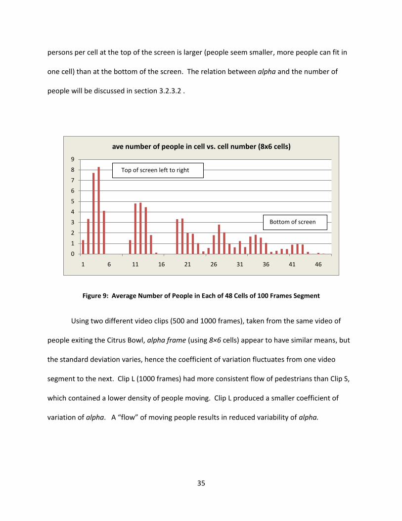
35

persons per cell at the top of the screen is larger (people seem smaller, more people can fit in

one cell) than at the bottom of the screen. The relation between alpha and the number of

people will be discussed in section ‎3.2.3.2 .

Figure 9: Average Number of People in Each of 48 Cells of 100 Frames Segment

Using two different video clips (500 and 1000 frames), taken from the same video of

people exiting the Citrus Bowl, alpha frame (using 8×6 cells) appear to have similar means, but

the standard deviation varies, hence the coefficient of variation fluctuates from one video

segment to the next. Clip L (1000 frames) had more consistent flow of pedestrians than Clip S,

which contained a lower density of people moving. Clip L produced a smaller coefficient of

variation of alpha. A “flow” of moving people results in reduced variability of alpha.

0

1

2

3

4

5

6

7

8

9

1 6 11 16 21 26 31 36 41 46

ave number of people in cell vs. cell number (8x6 cells)

Top of screen left to right

Bottom of screen

36

Alpha frame Clip L Clip S

Mean 0.0169 0.0164

Standard Deviation 0.00200 0.00417

Coefficient of Variation 0.118 0.255

Alpha frame, after removing cells containing zeros in the tracked velocities from the

summation of velocities used to calculate alpha, is shown below:

Alpha frame Clip L

Mean 0.0253

Standard Deviation 0.00324

Coefficient of Variation 0.128

On average, the mean and standard deviation of alpha increased and the coefficient of

variation was slightly higher after removing cells with no motion, in which alpha had been

arbitrarily taken to be zero. Comparing the changes more closely in short segments reveals

that though the average alpha is always larger after removing the zeros, yet the standard

deviation and the coefficient of variation are sporadically smaller. The parameter alpha-frame

for the two clips includes the cells with crowd flow and those without, and this phenomenon

varies from one video segment to the next, causing the variation in alpha frame.

3.1.3.2 Alpha of cell

Alpha cell is defined as:

. There is one alpha for each cell.

These are summed over a chosen number of frames, for example if summed for cell number 5,

for 100 frames, then there are 20 points (one every fifth frame). If we are using 8x6 cells, then

37

there are 48 of those sets of 20 points summations. The variation of these alphas from cell to

cell was found to be of the same order as that of alpha cell itself. This is caused by the large

fluctuation in the flow in the various cells, some have a crowd flow and some have no motion,

causing alpha cells to be so different. Calculating alpha cell for sets of 100 frame segments,

alpha cell still varied, for each cell, from segment to segment. The coefficient of variation for

this ranged from 0.166 in cells with consistent flow, to 3.16 in cells where there were people

walking only occasionally. Some cells, where there was no motion tracked, have an alpha = 0.

3.1.3.3 Alpha of array

One can also sum over all cells for several frames. This will give one alpha for a set of

frames. The array is the 48 cells × any number of frames. Since there is a practical limit on how

many frames can be processed manually to obtain the trajectories, combining all cells in a

number of frames together, will give only a small number of alpha-array as output.

3.1.3.4 Alpha of rows

While studying variations of alphas, it was observed that alpha had a systematic

variation within any frame. If the frame was divided into columns, alpha hardly varied from left

to right. However, when the frame was divided into rows, alpha changed with rows from top to

bottom. In frames with 8×6 cells there are 6 rows, numbered from 1 at top to 6 at bottom. To

calculate alpha of a row:

38

The change in alpha from one row to the next was more pronounced when there was a

nonzero steady crowd flow in one direction. The reason was hypothesized to be due to

geometric distortion. At the top row, people seem smaller (a smaller number of pixels per

person will be changing positions, affecting optical flow). At the same time, working in the

opposite direction, if a person at the bottom of the frame moves one step, possibly ten pixels,

the same person’s step at the top may be only 6 pixels (affecting velocities in both optical flow

and tracked trajectories). And since we are using the sum of the velocities in a cell for manually

tracked data, and more people can fit in one cell at the top than in a cell at the bottom, the

velocities will seem different in the different levels of the screen (in the results of Vtot of the

observed trajectories). The effect of the number of people in a cell is discussed in more detail

in the following ‘Results’ section.

3.2 Results

There are several variables to investigate to find the best conditions for the calibration

of optical flow to correspond to observed track velocities. Alpha, the proportionality parameter

varies depending on which restrictions are set when the experiments are run, for example, how

many frames are included or what optical flow settings were chosen. It would be advantageous

to find the parameter settings where alpha varies the least. Variation in data is usually

measured by how large their standard deviation is as compared to the mean.

39

During the course of preparing for the experiments, a decision had to be made as to

which alpha to use to proceed with the investigation. At that time, it was decided to choose

the alpha that had a lower coefficient of variation. This was the alpha calculated using Vtot of

the manual tracking. The experiments in this section were mostly carried out using results from

Vtot. Variation in alpha was found to be related to the number of people in the cells. Therefore,

some of these experiments were repeated later with Vave and are reported below.

The coefficient of variation of alpha frame, calculated using Vtot, under a variety of

conditions is shown in Table 1. These summary results were for the video of the Citrus Bowl

exit, using Lucas-Kanade optical flow. As can be seen, a lower coefficient of variation of alpha

was seen at a larger aperture of 15 and at smaller thresholds (red cells). The more pixel

structure that is used as input (larger aperture) and the finer, more detailed the picture (smaller

threshold), the lower the variation in alpha. Larger cells also show smaller variation. More

pixels are averaged over the larger cells, thus reducing the variability. Results of further

investigation of the different parameters are given next.

3.2.1 Details of Varying Lukas-Kanade Optical Flow Parameters

3.2.1.1 Thresholds

Thresholds serve to diminish the effect of noise on optical flow results. They smooth

the image. They can also convert a grayscale image to a bi-level or black-and-white image,

when needed, to be followed by finding contours (or edges) of intensity blobs. The effect of a

range of thresholds on a frame is shown in Figure 10. The OpenCV program using the Lukas-

Kanade method works on monochromatic pictures (gray-scale), giving rise to one set of light

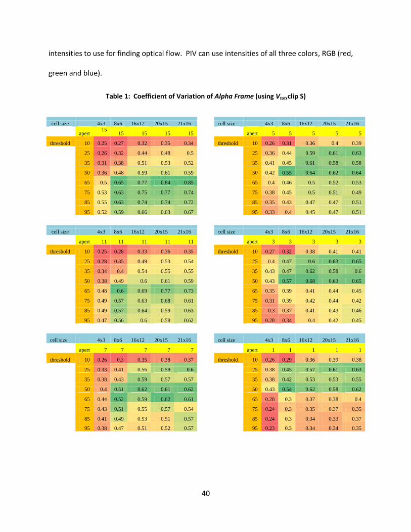
40

intensities to use for finding optical flow. PIV can use intensities of all three colors, RGB (red,

green and blue).

Table 1: Coefficient of Variation of Alpha Frame (using Vtot,clip S)

cell size 4x3 8x6 16x12 20x15 21x16 cell size 4x3 8x6 16x12 20x15 21x16

apert 15

15 15 15 15 apert 5 5 5 5 5

threshold 10 0.25 0.27 0.32 0.35 0.34 threshold 10 0.26 0.31 0.36 0.4 0.39

25 0.26 0.32 0.44 0.48 0.5 25 0.36 0.44 0.59 0.61 0.63

35 0.31 0.38 0.51 0.53 0.52 35 0.41 0.45 0.61 0.58 0.58

50 0.36 0.48 0.59 0.61 0.59 50 0.42 0.55 0.64 0.62 0.64

65 0.5 0.65 0.77 0.84 0.85 65 0.4 0.46 0.5 0.52 0.53

75 0.53 0.63 0.75 0.77 0.74 75 0.38 0.45 0.5 0.51 0.49

85 0.55 0.63 0.74 0.74 0.72 85 0.35 0.43 0.47 0.47 0.51

95 0.52 0.59 0.66 0.63 0.67 95 0.33 0.4 0.45 0.47 0.51


apert 11 11 11 11 11 apert 3 3 3 3 3


25 0.28 0.35 0.49 0.53 0.54 25 0.4 0.47 0.6 0.63 0.65

35 0.34 0.4 0.54 0.55 0.55 35 0.43 0.47 0.62 0.58 0.6

50 0.38 0.49 0.6 0.61 0.59 50 0.43 0.57 0.68 0.63 0.65

65 0.48 0.6 0.69 0.77 0.73 65 0.35 0.39 0.41 0.44 0.45

75 0.49 0.57 0.63 0.68 0.61 75 0.31 0.39 0.42 0.44 0.42

85 0.49 0.57 0.64 0.59 0.63 85 0.3 0.37 0.41 0.43 0.46

95 0.47 0.56 0.6 0.58 0.62 95 0.28 0.34 0.4 0.42 0.45


apert 7 7 7 7 7 apert 1 1 1 1 1


25 0.33 0.41 0.56 0.59 0.6 25 0.38 0.45 0.57 0.61 0.63

35 0.38 0.43 0.59 0.57 0.57 35 0.38 0.42 0.53 0.53 0.55

50 0.4 0.51 0.62 0.61 0.62 50 0.43 0.54 0.62 0.58 0.62

65 0.44 0.52 0.59 0.62 0.61 65 0.28 0.3 0.37 0.38 0.4

75 0.43 0.51 0.55 0.57 0.54 75 0.24 0.3 0.35 0.37 0.35

85 0.41 0.49 0.53 0.51 0.57 85 0.24 0.3 0.34 0.33 0.37

95 0.38 0.47 0.51 0.52 0.57 95 0.23 0.3 0.34 0.34 0.35

41

Results of testing alpha frames at various thresholds are shown in Table 1 and Figure

11. Small thresholds show smaller coefficients of variation at all apertures except aperture = 1

(in Table 1, red is smaller values, green is larger). At aperture 1, there are two regions with

small coefficients of variation. As one can see from the snapshots in Figure 10, the detail of the

picture is lost at higher thresholds. Thresholds near zero have consistently low alpha variation.

The reason for higher values in the variation of alpha could be because, on average, alpha itself

is much smaller at higher thresholds, as shown in Figure 12.

Original Frame

Threshold 10

Threshold 25

Threshold 50

Threshold 75

Threshold 90

Figure 10: Video Frame as It Appears After Using Various Thresholds

42

1

15

00

5

10

0

15

550

100

0

2.5

5

7.5

10

12.5

coeff of var

Aperture

Threshold

Coefficient of variation of Alpha vs Aperture, Threshold (clip S)

Figure 11: Variation of Alpha of Frames with Aperture and Threshold

4003002001000

0.0200

0.0175

0.0150

0.0125

0.0100

0.0075

0.0050

frames

alp

ha

fra

me

s

Thresh 1

Thresh 10

Thresh 25

Thresh 35

Thresh 50

Thresh 65

Thresh75

Thresh 85

Variable

Alpha frames vs frames for various thresholds at aperture = 15

Figure 12: Variation of Average of Alpha with Time at Various Thresholds (Clip S)

43

3.2.1.2 Aperture

The aperture is the area around a pixel, where the program looks for a blob of similar

light intensity in the later frame. When the aperture is small, and all the pixels within the

aperture are of similar intensity, one cannot detect the direction of movement. Furthermore,

the movement could easily be so large, that within the aperture, the program cannot find a

good correspondence between areas of similar intensity. When the aperture is too large, one

could detect two motions in different directions in the same aperture window. Which direction

will the optical flow calculations find to have the least error or best correlation?

From Table 1, alpha has a consistently small coefficient of variation around the top left

corner at apertures 15, 11 and 7, where the threshold is small. This region shrinks at apertures

5, 3 and 1, and another region appears at high thresholds. High thresholds, however, lose a lot

of the detail of the image, and would not be suitable if there is a large crowd with many people

overlapping. Figure 13 shows that on average, alpha is higher at larger apertures. This

contributes to the smaller coefficient of variation at aperture 15. The decision was made to use

a large aperture combined with a small threshold for the remainder of the research. Most of

the experiments were conducted at aperture 15, threshold 10, and cell size 8×6, unless

otherwise noted.

44

4003002001000

0.020

0.019

0.018

0.017

0.016

0.015

0.014

0.013

0.012

0.011

frames

alp

ha

fra

me

sApert 3

Apert 5

Apert 7

Apert 11

Apert 15

Variable

Alpha frames vs frames for various apertures at threshold=10

Figure 13: Variation of Average of Alpha with Frames at Various Apertures (Clip S)

3.2.2 Varying Manual Tracking Parameters

3.2.2.1 Velocity: Sum versus Average

One can use the sum of tracked velocities in a cell, or their average, when comparing

them to optical flow. Alpha frame was calculated using both methods. Figure 14 shows that in

this clip of close to a thousand frames, when using the total velocity, the resulting alpha is more

scattered than when using average velocity. However, since the mean of alpha calculated from

the average velocity is smaller, its coefficient of variation may not always be smaller.

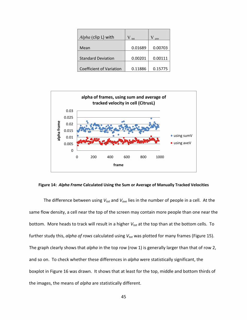
45

Alpha (clip L) with V tot V ave

Mean 0.01689 0.00703

Standard Deviation 0.00201 0.00111

Coefficient of Variation 0.11886 0.15775

Figure 14: Alpha Frame Calculated Using the Sum or Average of Manually Tracked Velocities

The difference between using Vtot and Vave lies in the number of people in a cell. At the

same flow density, a cell near the top of the screen may contain more people than one near the

bottom. More heads to track will result in a higher Vtot at the top than at the bottom cells. To

further study this, alpha of rows calculated using Vtot was plotted for many frames (Figure 15).

The graph clearly shows that alpha in the top row (row 1) is generally larger than that of row 2,

and so on. To check whether these differences in alpha were statistically significant, the

boxplot in Figure 16 was drawn. It shows that at least for the top, middle and bottom thirds of

the images, the means of alpha are statistically different.

0

0.005

0.01

0.015

0.02

0.025

0.03

0 200 400 600 800 1000

alp

ha

fram

e

frame

alpha of frames, using sum and average of tracked velocity in cell (CitrusL)

using sumV

using aveV

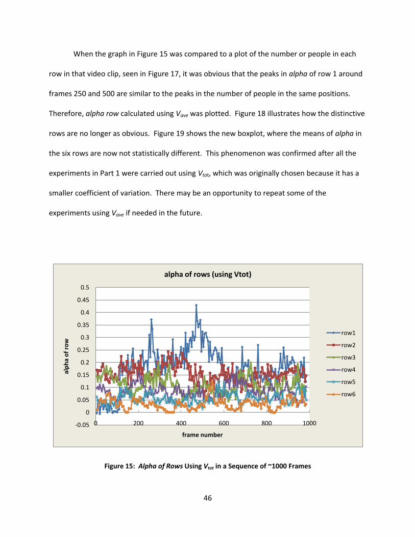
46

When the graph in Figure 15 was compared to a plot of the number or people in each

row in that video clip, seen in Figure 17, it was obvious that the peaks in alpha of row 1 around

frames 250 and 500 are similar to the peaks in the number of people in the same positions.

Therefore, alpha row calculated using Vave was plotted. Figure 18 illustrates how the distinctive

rows are no longer as obvious. Figure 19 shows the new boxplot, where the means of alpha in

the six rows are now not statistically different. This phenomenon was confirmed after all the

experiments in Part 1 were carried out using Vtot, which was originally chosen because it has a

smaller coefficient of variation. There may be an opportunity to repeat some of the

experiments using Vave if needed in the future.

Figure 15: Alpha of Rows Using Vtot in a Sequence of ~1000 Frames

-0.05

0

0.05

0.1

0.15

0.2

0.25

0.3

0.35

0.4

0.45

0.5

0 200 400 600 800 1000

alp

ha

of

row

frame number

alpha of rows (using Vtot)

row1

row2

row3

row4

row5

row6

47

Figure 16: Boxplot of Alpha Row Calculated Using Vtot

Figure 17: Number of People in a Row, in a Sequence of ~1000 Frames

row6row5row4row3row2row1

0.08

0.07

0.06

0.05

0.04

0.03

0.02

0.01

0.00

Da

ta

Boxplot of row1, row2, row3, row4, row5, row6

0

5

10

15

20

25

30

35

40

0 200 400 600 800 1000

nu

mb

er

of

pe

op

le

frames

Number of People in row (clip L)

row 1

row 2

row 3

row 4

row 5

row 6

48

Figure 18: Alpha of Rows Using Vave in a Sequence of ~1000 Frames

row6row5row4row3row2row1

0.016

0.014

0.012

0.010

0.008

0.006

0.004

0.002

0.000

Da

ta

Boxplot of row1, row2, row3, row4, row5, row6

Figure 19: Boxplot of Alpha Row Calculated Using Vave

-0.002

0

0.002

0.004

0.006

0.008

0.01

0.012

0.014

0.016

0 200 400 600 800 1000 1200

alp

ha

of

row

s

frame

alpha of rows (using Vtot)

row1

row2

row3

row4

row5

row6

49

3.2.2.2 Spreading Manual Tracking Data

When manually tracking the path of individuals in a video, the researcher marks the

position of a person by one crosshair marker on the head. Screen velocities are calculated by

comparing the positions of these markers. In contrast, optical flow programs detect the

movement of all the pixels occupied by that person. Assuming that the entire body of a person

moves at identical speed, and disregarding the different leg and arm motion, a program was

written to spread the velocity of a person, from being assigned to one pixel, to being

distributed over a rectangle. For the Citrus Bowl exit video, a rectangle 10x25 pixels was

chosen, which is comparable to the average width × height of a person in the middle of the

video screen. Figure 20 shows the rectangle over which the velocity is spread.

Figure 20: Velocity of an Individual Is Spread from One Pixel (Red) to a Rectangle 10x25

1 2 3 4 5 6 7 8 9 10

2

3

4

5

6

7

8

9

10

11

12

13

14

15

16

17

18

19

20

21

22

23

24

25

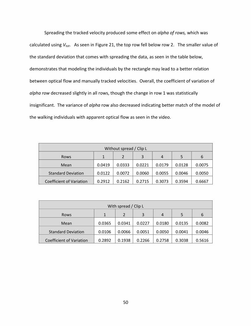
50

Spreading the tracked velocity produced some effect on alpha of rows, which was

calculated using Vtot. As seen in Figure 21, the top row fell below row 2. The smaller value of

the standard deviation that comes with spreading the data, as seen in the table below,

demonstrates that modeling the individuals by the rectangle may lead to a better relation

between optical flow and manually tracked velocities. Overall, the coefficient of variation of

alpha row decreased slightly in all rows, though the change in row 1 was statistically

insignificant. The variance of alpha row also decreased indicating better match of the model of

the walking individuals with apparent optical flow as seen in the video.

Without spread / Clip L

Rows 1 2 3 4 5 6

Mean 0.0419 0.0333 0.0221 0.0179 0.0128 0.0075

Standard Deviation 0.0122 0.0072 0.0060 0.0055 0.0046 0.0050

Coefficient of Variation 0.2912 0.2162 0.2715 0.3073 0.3594 0.6667

With spread / Clip L

Rows 1 2 3 4 5 6

Mean 0.0365 0.0341 0.0227 0.0180 0.0135 0.0082

Standard Deviation 0.0106 0.0066 0.0051 0.0050 0.0041 0.0046

Coefficient of Variation 0.2892 0.1938 0.2266 0.2758 0.3038 0.5616

51

Figure 21: Alpha Rows (L-K) after Spreading Manual Tracking Data

3.2.3 Varying Experiment Parameters

3.2.3.1 Cell Size

In each frame, optical flow obtains a velocity value for each pixel. These velocity values

were then averaged into cells. Alpha is calculated using the velocity components in the x and y

direction, averaged for cells. The averaging was also performed using the total velocity tracked

manually. The question arose as to whether alpha would vary less if the cell size was the same

as the size of the optical flow aperture. That was found not to be true. In the Citrus Bowl

video, alpha for cell size 40 x 40 varied less than that for cell size 15 x 15. Figure 22 shows that,

in general, the coefficient of variation of alpha decreases with cell size up to about size 40x40,

when it levels out. It would be unnecessary to divide the frame into smaller cells requiring

more calculations, if the coefficient of variation of alpha does not improve further.

0

0.01

0.02

0.03

0.04

0.05

0.06

0.07

0.08

0 200 400 600 800 1000

alp

ha

of

row

s

segment of 100 frames

ave of 100 frame segments of alpha of rows , spread MT, Clip L

row1

row2

row3

row4

row5

row6

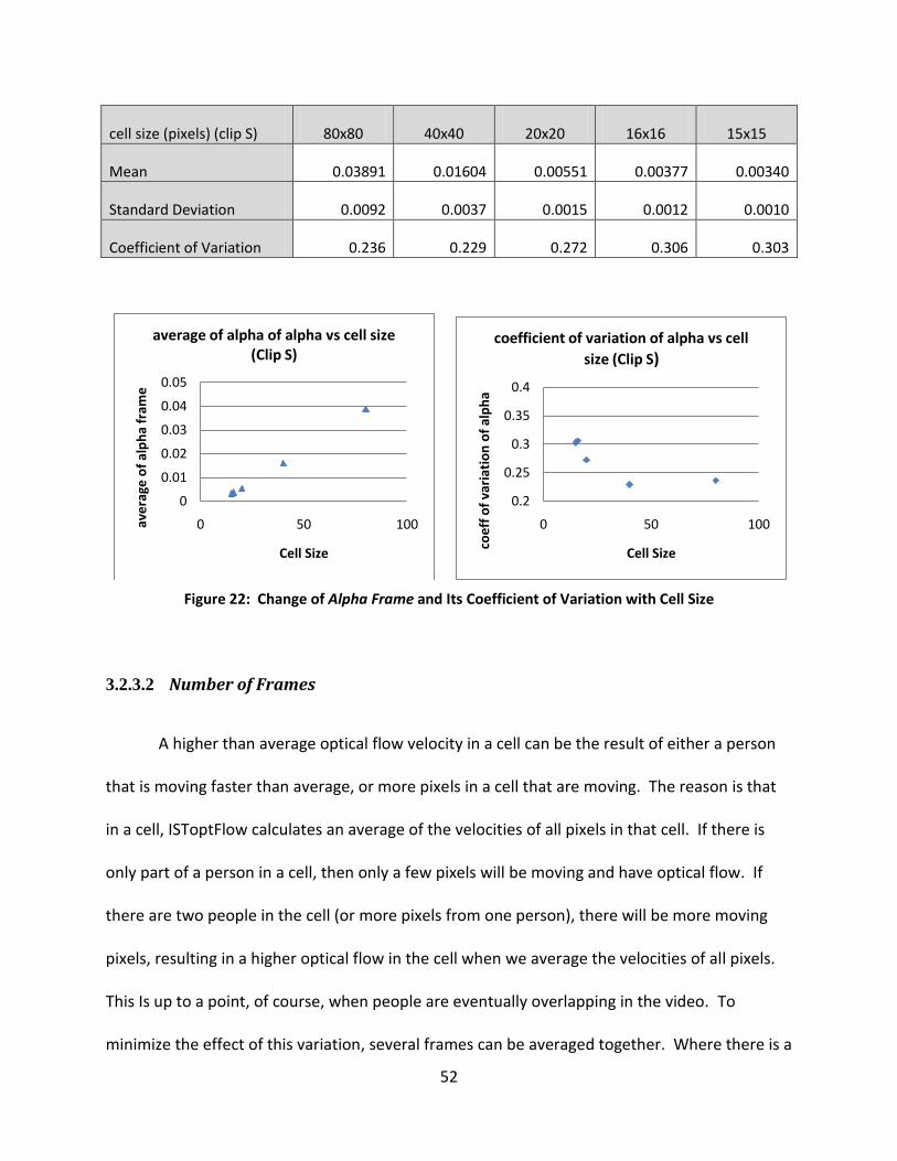
52

cell size (pixels) (clip S) 80x80 40x40 20x20 16x16 15x15

Mean 0.03891 0.01604 0.00551 0.00377 0.00340

Standard Deviation 0.0092 0.0037 0.0015 0.0012 0.0010

Coefficient of Variation 0.236 0.229 0.272 0.306 0.303

Figure 22: Change of Alpha Frame and Its Coefficient of Variation with Cell Size

3.2.3.2 Number of Frames

A higher than average optical flow velocity in a cell can be the result of either a person

that is moving faster than average, or more pixels in a cell that are moving. The reason is that

in a cell, ISToptFlow calculates an average of the velocities of all pixels in that cell. If there is

only part of a person in a cell, then only a few pixels will be moving and have optical flow. If

there are two people in the cell (or more pixels from one person), there will be more moving

pixels, resulting in a higher optical flow in the cell when we average the velocities of all pixels.

This Is up to a point, of course, when people are eventually overlapping in the video. To

minimize the effect of this variation, several frames can be averaged together. Where there is a

0

0.01

0.02

0.03

0.04

0.05

0 50 100ave

rage

of

alp

ha

fram

e

Cell Size

average of alpha of alpha vs cell size (Clip S)

0.2

0.25

0.3

0.35

0.4

0 50 100

coe

ff o

f va

riat

ion

of

alp

ha

Cell Size

coefficient of variation of alpha vs cell

size (Clip S)

53

steady flow of people, an average flow velocity appears and is more evenly distributed as

opposed to the jagged distribution of separate individuals that enter and leave a cell over a few

frames’ time. The differences between the values in the cells of single frames and averaged

frames of manually tracked and optical flow data are shown in Figure 23.

LK Optical Flow in One Frame LK Optical Flow Averaged Over 100 Frames

Observed Trajectories in One Frame Observed Trajectories Averaged over 100 Frames

Figure 23: Vx of Optical Flow and Observed Trajectories, 20 X15 Cells, Single and Averaged Frames

The color coding is for visual clarity, where red is a smaller number (negative direction)

and green is larger and yellow is near zero. Red cells indicate a movement in the negative x-

direction, to the left. Data is recorded every fifth frame. An average of 100 frames is 20 data

points. It is obvious if we are comparing the two frames on the left, one set of frames in optical

f rame 70 frame 70 to #

Vx 0 1 2 3 4 5 6 7 8 9 10 11 12 13 14 15 16 17 18 19 Vx 0 1 2 3 4 5 6 7 8 9 10 11 12 13 14 15 16 17 18 19

0 1 1 1 1 0

1 1 1 1 1

2 1 1 2

3 1 1 1 3

4 1 1 1 1 4

5 5 1 1

6 1 1 6

7 1 1 7

8 1 8

9 1 1 1 9

10 10

11 1 11

12 1 12

13 13

14 14

frame 70 frame 70 to #

Vx 0 1 2 3 4 5 6 7 8 9 10 11 12 13 14 15 16 17 18 19 Vx 0 1 2 3 4 5 6 7 8 9 10 11 12 13 14 15 16 17 18 19

0 0

1 1

2 2

3 3 1

4 4

5 5 1 1

6 6 1 1 1

7 1 7 1 1

8 1 8 1

9 1 1 1 9 1 1

10 1 1 1 10 1 1

11 1 1 1 11 1 1

12 1 12 1 1 1

13 1 13 1 1 1

14 14 1

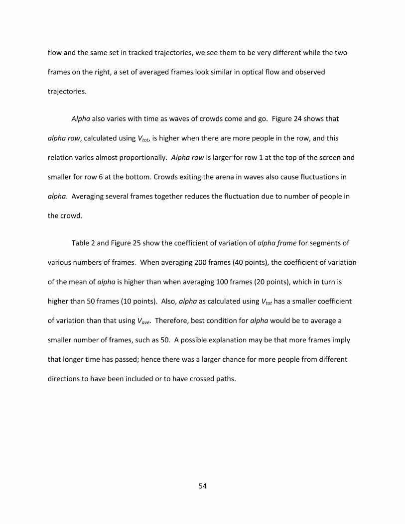
54

flow and the same set in tracked trajectories, we see them to be very different while the two

frames on the right, a set of averaged frames look similar in optical flow and observed

trajectories.

Alpha also varies with time as waves of crowds come and go. Figure 24 shows that

alpha row, calculated using Vtot, is higher when there are more people in the row, and this

relation varies almost proportionally. Alpha row is larger for row 1 at the top of the screen and

smaller for row 6 at the bottom. Crowds exiting the arena in waves also cause fluctuations in

alpha. Averaging several frames together reduces the fluctuation due to number of people in

the crowd.

Table 2 and Figure 25 show the coefficient of variation of alpha frame for segments of

various numbers of frames. When averaging 200 frames (40 points), the coefficient of variation

of the mean of alpha is higher than when averaging 100 frames (20 points), which in turn is

higher than 50 frames (10 points). Also, alpha as calculated using Vtot has a smaller coefficient

of variation than that using Vave. Therefore, best condition for alpha would be to average a

smaller number of frames, such as 50. A possible explanation may be that more frames imply

that longer time has passed; hence there was a larger chance for more people from different

directions to have been included or to have crossed paths.

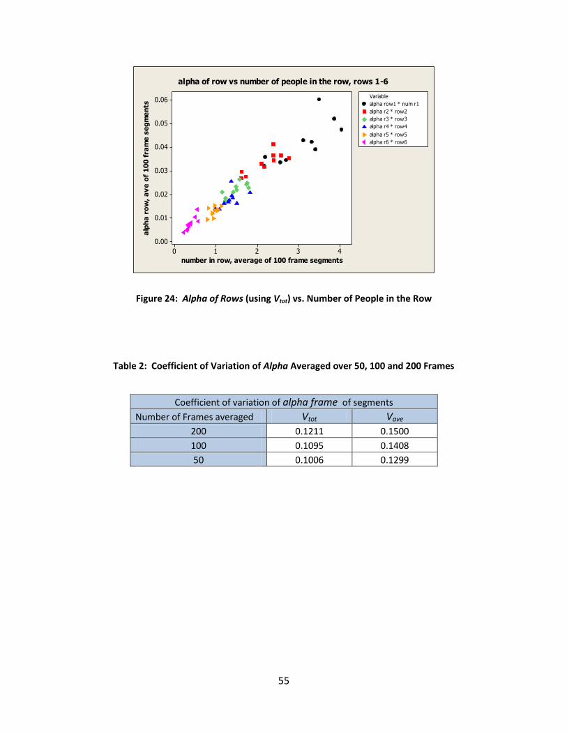
55

43210

0.06

0.05

0.04

0.03

0.02

0.01

0.00

number in row, average of 100 frame segments

alp

ha

ro

w,

av

e o

f 1

00

fra

me

se

gm

en

ts alpha row1 * num r1

alpha r2 * row2

alpha r3 * row3

alpha r4 * row4

alpha r5 * row5

alpha r6 * row6

Variable

alpha of row vs number of people in the row, rows 1-6

Figure 24: Alpha of Rows (using Vtot) vs. Number of People in the Row

Table 2: Coefficient of Variation of Alpha Averaged over 50, 100 and 200 Frames

Coefficient of variation of alpha frame of segments

Number of Frames averaged Vtot Vave

200 0.1211 0.1500

100 0.1095 0.1408

50 0.1006 0.1299

56

Figure 25: Average Coefficient of Variation of Alpha of Frames for Segments of Various Numbers of Averaged Frames

3.2.3.3 Cutoff

The video used in this thesis has a crowd moving through a gate, and places where there

is no movement, beyond the fence where the gate is located. The areas with no people

walking, for example where there is a fence or a tree, show up as having zero velocity in the

data of tracked paths, even over a number of frames. In the optical flow data, however, these

areas may have small velocity values. These arise from light and shadow movement, tree

branches swaying, or other background flickering noise. The result is that the tracked

trajectories data does not perfectly match the optical flow data. Two methods could be used to

alleviate the problem.

0.1000

0.1100

0.1200

0.1300

0.1400

0.1500

0.1600

0 50 100 150 200 250

Ave

Co

eff

of

Var

n

Num of Frames Averaged

Average Coefficient of Variation of Alpha Framefor 50, 100, 200 frame segments, Vave & Vtot

ave coeff of varn (Vtot)

ave coeff of varn (Vave)

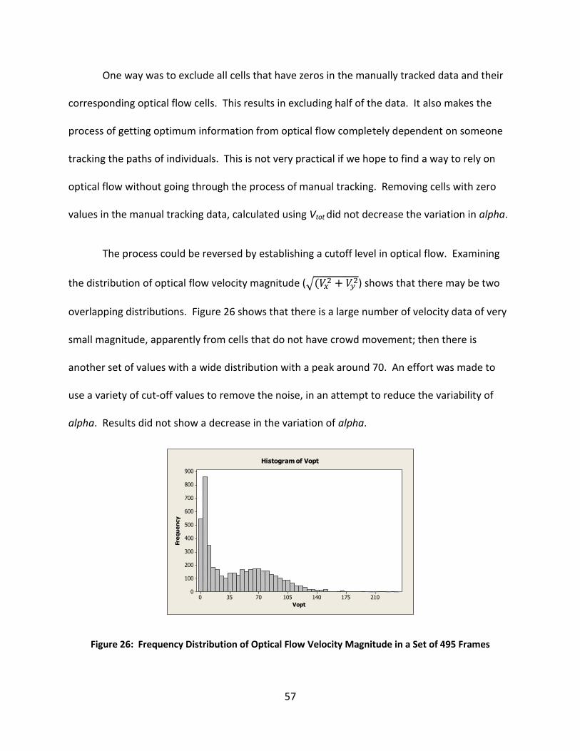
57

One way was to exclude all cells that have zeros in the manually tracked data and their

corresponding optical flow cells. This results in excluding half of the data. It also makes the

process of getting optimum information from optical flow completely dependent on someone

tracking the paths of individuals. This is not very practical if we hope to find a way to rely on

optical flow without going through the process of manual tracking. Removing cells with zero

values in the manual tracking data, calculated using Vtot did not decrease the variation in alpha.

The process could be reversed by establishing a cutoff level in optical flow. Examining

the distribution of optical flow velocity magnitude ( ) shows that there may be two

overlapping distributions. Figure 26 shows that there is a large number of velocity data of very

small magnitude, apparently from cells that do not have crowd movement; then there is

another set of values with a wide distribution with a peak around 70. An effort was made to

use a variety of cut-off values to remove the noise, in an attempt to reduce the variability of

alpha. Results did not show a decrease in the variation of alpha.

21017514010570350

900

800

700

600

500

400

300

200

100

0

Vopt

Fre

qu

en

cy

Histogram of Vopt

Figure 26: Frequency Distribution of Optical Flow Velocity Magnitude in a Set of 495 Frames

58

3.2.3.4 Center Cells

It is better to perform a smaller number of calculations when possible, conserving

computer processing time. Therefore, it is of benefit to use any physical constraints available to

reduce the data that has to be processed. In an image sequence such as that of the Citrus Bowl

exit, the area of the image under investigation will differ depending on the output required. If

the required output was the velocity vector to study how the speed possibly slows down at the

crowded exit, then the areas of the image showing people moving at normal speed, then

slowing at the gate, and resuming normal speed beyond the gate, need to be included. If,

however, optical flow is used to estimate the number of people exiting, then it is enough to

include the data of the few cells covering the gate area, which are called herein “center cells”.

Similarly, if the video is of a crowd moving in a corridor with no side exits, then it should be

sufficient to choose one section as the investigation area.

The center cells of a frame that is divided into 8x6 cells are shown in Figure 27. This is

where the crowd flow is denser and more consistent. Table 3 and Figure 28 show that when

using Vtot to calculate alpha, there is a large difference between alpha of frame and alpha of

center-cells. The reason is that the crowd is denser within the confines of the gate. The

number of people in the cells is reflected in alpha, and averaging alphas in center-cells only

results in a higher mean. When using Vave, however, this phenomenon disappears and the two

alphas are very close in both mean and coefficient of variation. There is, however, another

factor at work.

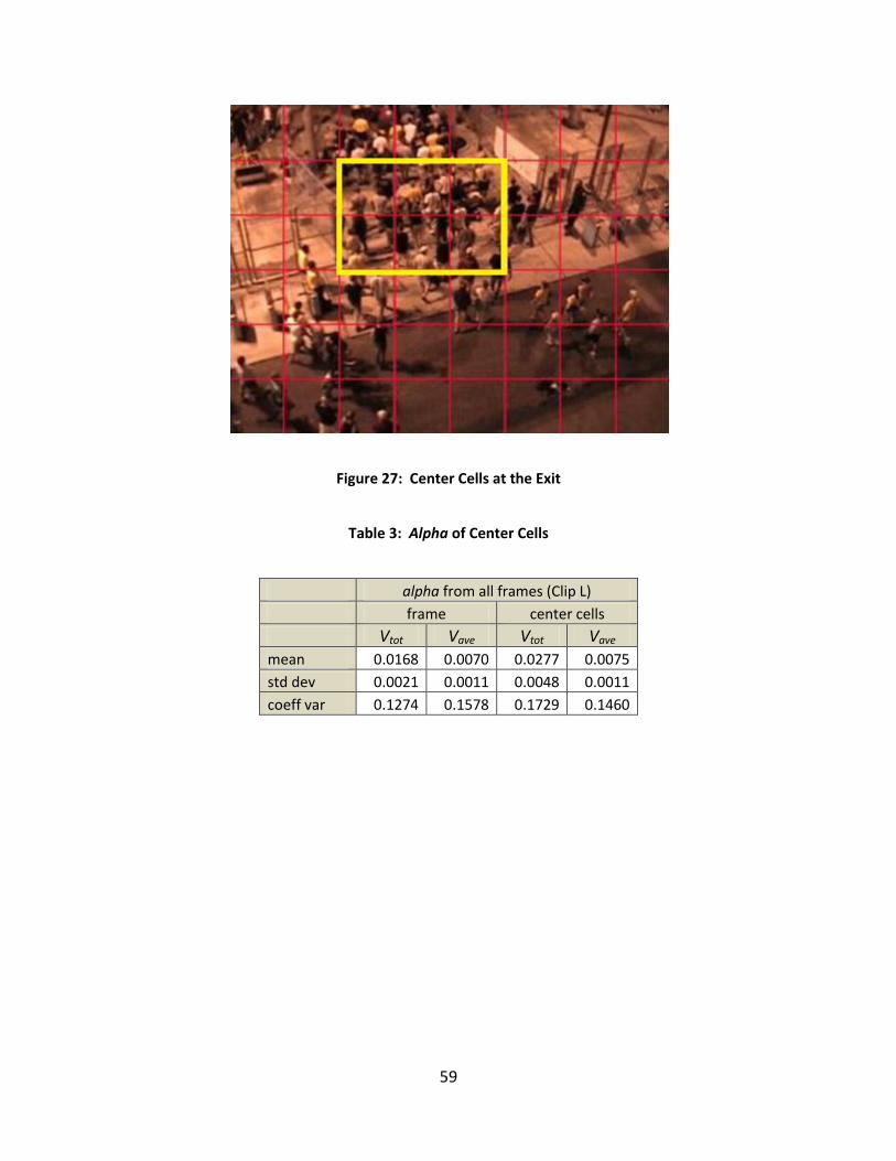
59

Figure 27: Center Cells at the Exit

Table 3: Alpha of Center Cells

alpha from all frames (Clip L)

frame center cells

Vtot Vave Vtot Vave

mean 0.0168 0.0070 0.0277 0.0075

std dev 0.0021 0.0011 0.0048 0.0011

coeff var 0.1274 0.1578 0.1729 0.1460

60

Figure 28: Alpha calculated from Sums of All Cells in the Frame and from Center Cells

Figure 29 and Figure 30 show the average of Vx and Vy separately. These frames were

divided into 40x30 cells. After averaging 985 frames, Vx in the center cells canceled out and

there is an area of very small values (yellow). The motion in the center cells is both to the left

and to the right into the gate, while people exit the building from one side and walk towards

parking on another side, so Vx canceled out. This affects the later use of alpha to predict flow.

Flow in one direction, such as Vy in Figure 30, shows less inaccuracy; however this cannot be

controlled in actual situations.

0

0.005

0.01

0.015

0.02

0.025

0.03

0.035

0 500 1000 1500

Ave alpha of 100 frame segments center cell, alpha frame and center-cells

ave alpha frame, 100 fr segments, Vtot

ave alpha frame, 100 fr segments, Vave

Ave alpha of 100 frame segments ctr Vtot

Ave alpha of 100 frame segments ctr Vave

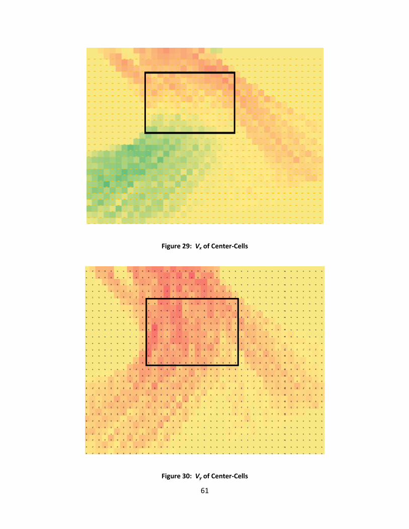
61

Figure 29: Vx of Center-Cells

Figure 30: Vy of Center-Cells

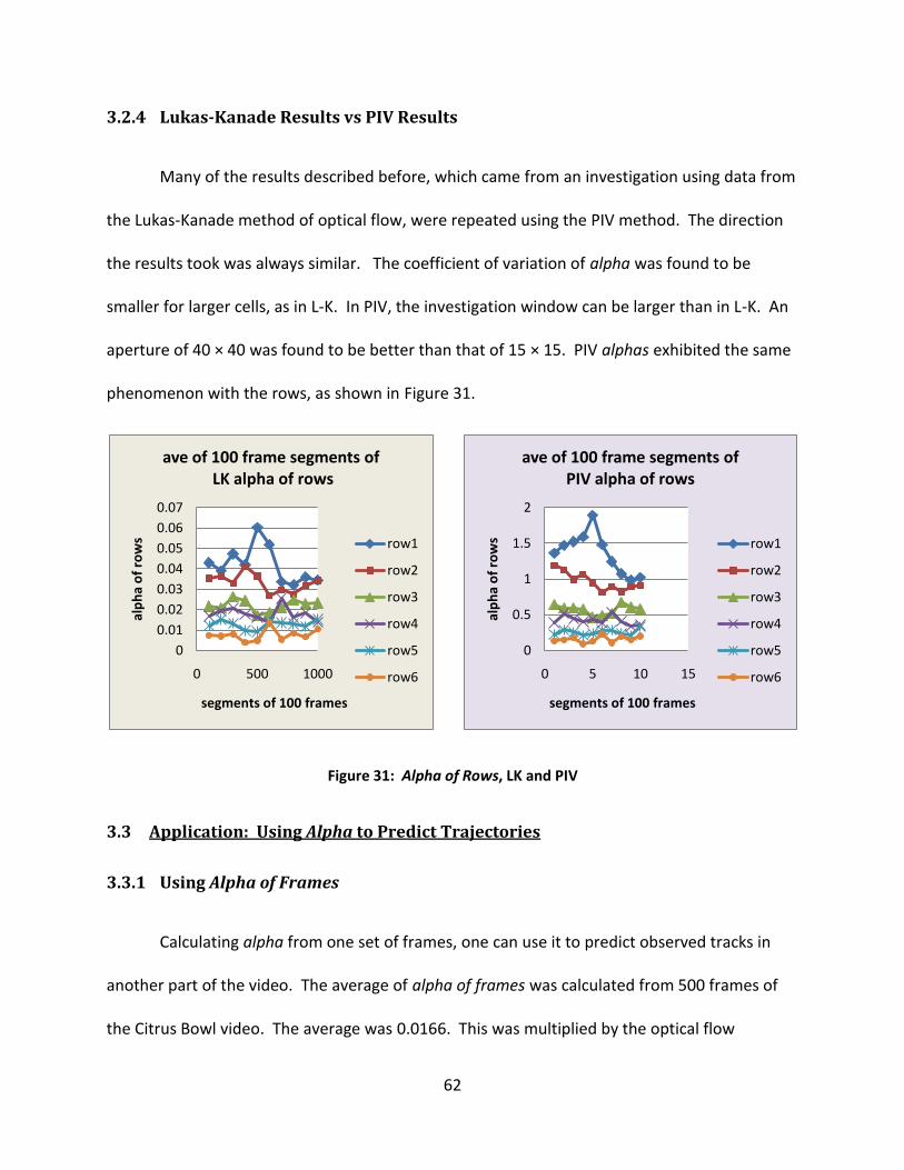
62

3.2.4 Lukas-Kanade Results vs PIV Results

Many of the results described before, which came from an investigation using data from

the Lukas-Kanade method of optical flow, were repeated using the PIV method. The direction

the results took was always similar. The coefficient of variation of alpha was found to be

smaller for larger cells, as in L-K. In PIV, the investigation window can be larger than in L-K. An

aperture of 40 × 40 was found to be better than that of 15 × 15. PIV alphas exhibited the same

phenomenon with the rows, as shown in Figure 31.

Figure 31: Alpha of Rows, LK and PIV

3.3 Application: Using Alpha to Predict Trajectories

3.3.1 Using Alpha of Frames

Calculating alpha from one set of frames, one can use it to predict observed tracks in

another part of the video. The average of alpha of frames was calculated from 500 frames of

the Citrus Bowl video. The average was 0.0166. This was multiplied by the optical flow

0

0.01

0.02

0.03

0.04

0.05

0.06

0.07

0 500 1000

alp

ha

of

row

s

segments of 100 frames

ave of 100 frame segments ofLK alpha of rows

row1

row2

row3

row4

row5

row6

0

0.5

1

1.5

2

0 5 10 15

alp

ha

of

row

s

segments of 100 frames

ave of 100 frame segments ofPIV alpha of rows

row1

row2

row3

row4

row5

row6

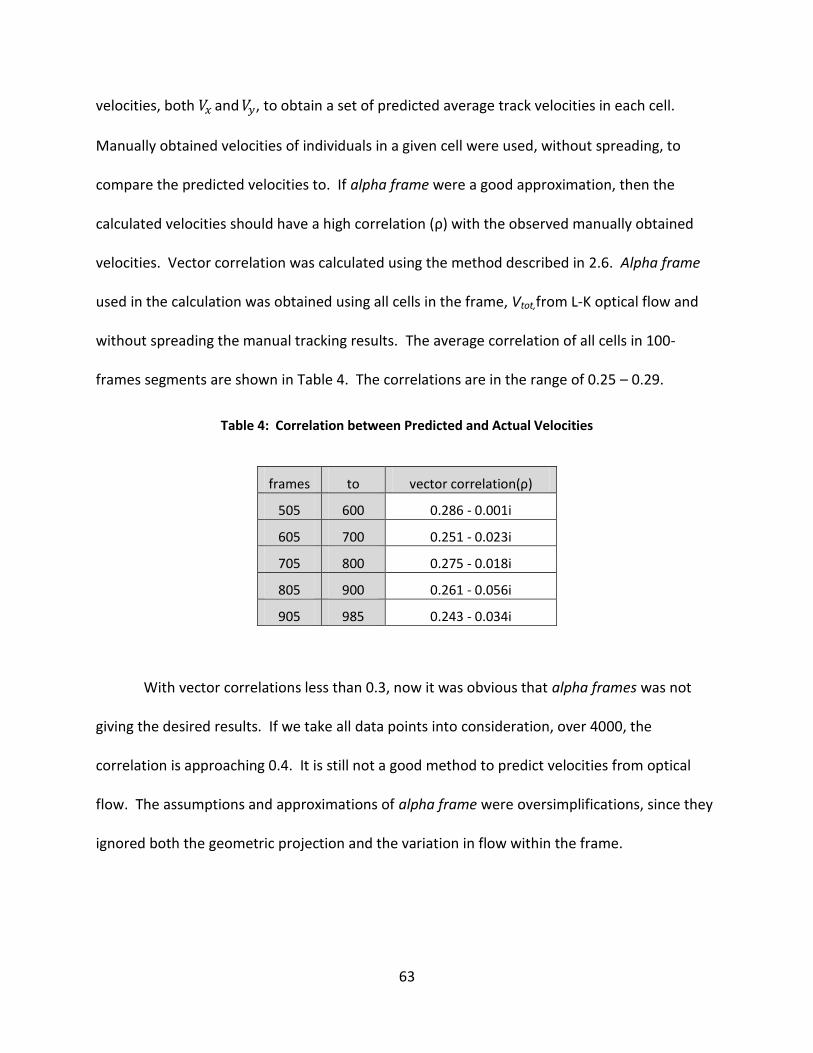
63

velocities, both and , to obtain a set of predicted average track velocities in each cell.

Manually obtained velocities of individuals in a given cell were used, without spreading, to

compare the predicted velocities to. If alpha frame were a good approximation, then the

calculated velocities should have a high correlation (ρ) with the observed manually obtained

velocities. Vector correlation was calculated using the method described in ‎2.6. Alpha frame

used in the calculation was obtained using all cells in the frame, Vtot,from L-K optical flow and

without spreading the manual tracking results. The average correlation of all cells in 100-

frames segments are shown in Table 4. The correlations are in the range of 0.25 – 0.29.

Table 4: Correlation between Predicted and Actual Velocities

frames to vector correlation(ρ)

505 600 0.286 - 0.001i

605 700 0.251 - 0.023i

705 800 0.275 - 0.018i

805 900 0.261 - 0.056i

905 985 0.243 - 0.034i

With vector correlations less than 0.3, now it was obvious that alpha frames was not

giving the desired results. If we take all data points into consideration, over 4000, the

correlation is approaching 0.4. It is still not a good method to predict velocities from optical

flow. The assumptions and approximations of alpha frame were oversimplifications, since they

ignored both the geometric projection and the variation in flow within the frame.

64

3.3.2 Using Alpha Rows

As the perspective view is definitely a factor in causing the low correlation between

screen optical flow and observed trajectories, similar predictions as above were computed

using alpha of rows. Knowing that alpha did not change much from left to right, but it changed

from top to bottom, an alpha was calculated for each of the six rows in an 8×6 cell frame, then

alpha of each row was averaged for 500 frames. Optical flow from a second set of frames was

multiplied by the corresponding alpha row, depending on its location. The correlation between

the averages of all data points of predicted and observed velocities rose up to 0.5.

3.3.3 Using Alpha of Cells

As the variation of flow in the different regions on the frame is also a factor, alpha of

cells was used to make predictions. This takes care of the position in the frame (the geometry),

and of whether the area has pedestrians walking or not (the flow). An alpha was calculated for

each of the 48 cells (8×6), and an average alpha cell found for the first 500 frames. Data to

calculate alpha came from utilizing Vtot,from L-K optical flow and without spreading the manual

tracking results. Optical flow and in a cell were each multiplied by the corresponding

alpha of that cell. This was compared to observed velocities from the second set of 500 frames.

Table 5 shows the real and imaginary parts of the correlation in each of the forty eight cells.

Their real value is largest (~1) where there are no people moving at all. They are smallest

where the video shows people’s paths cross. If the correlation is calculated using the sum of all

cells and all frames together, the real part is about 0.66 and the imaginary part is very small.

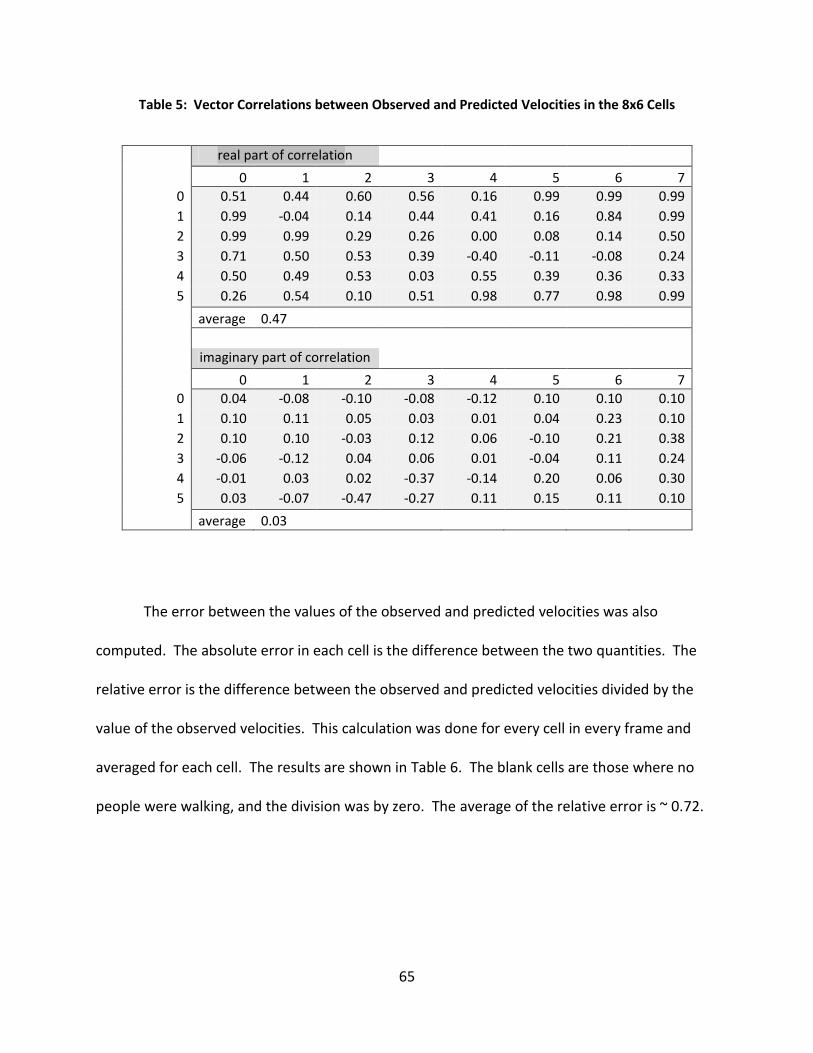
65

Table 5: Vector Correlations between Observed and Predicted Velocities in the 8x6 Cells

real part of correlation

0 1 2 3 4 5 6 7

0 0.51 0.44 0.60 0.56 0.16 0.99 0.99 0.99

1 0.99 -0.04 0.14 0.44 0.41 0.16 0.84 0.99

2 0.99 0.99 0.29 0.26 0.00 0.08 0.14 0.50

3 0.71 0.50 0.53 0.39 -0.40 -0.11 -0.08 0.24

4 0.50 0.49 0.53 0.03 0.55 0.39 0.36 0.33

5 0.26 0.54 0.10 0.51 0.98 0.77 0.98 0.99

average 0.47

imaginary part of correlation

0 1 2 3 4 5 6 7

0 0.04 -0.08 -0.10 -0.08 -0.12 0.10 0.10 0.10

1 0.10 0.11 0.05 0.03 0.01 0.04 0.23 0.10

2 0.10 0.10 -0.03 0.12 0.06 -0.10 0.21 0.38

3 -0.06 -0.12 0.04 0.06 0.01 -0.04 0.11 0.24

4 -0.01 0.03 0.02 -0.37 -0.14 0.20 0.06 0.30

5 0.03 -0.07 -0.47 -0.27 0.11 0.15 0.11 0.10

average 0.03

The error between the values of the observed and predicted velocities was also

computed. The absolute error in each cell is the difference between the two quantities. The

relative error is the difference between the observed and predicted velocities divided by the

value of the observed velocities. This calculation was done for every cell in every frame and

averaged for each cell. The results are shown in Table 6. The blank cells are those where no

people were walking, and the division was by zero. The average of the relative error is ~ 0.72.

66

Table 6: Relative Error between Observed and Predicted Tracks using Alpha-Cell

0.62 0.89 0.93 0.57 0.63

0.53 0.95 0.57 0.68 0.64 0.99

1.00 0.48 0.59 0.69 0.91 0.60 0.88

0.69 0.57 0.57 0.56 0.70 0.48 0.68 0.63

0.56 0.53 0.60 0.78 0.92 0.83 0.61 0.85

0.60 0.59 0.81 0.99

0.96 0.94

Alpha cell produced the best correlation of the three alphas. The Lukas-Kanade optical

flow varies greatly from frame to frame. And, even though, on average, its optical flow vectors

“looked like” they matched the motion of the crowd well, yet individual frames did not. Note

that if two vectors are of equal length but separated by 60 degrees, the relative error is 1.00

since you have an equilateral triangle consisting of the two vectors and their difference.

Similarly, a complete anti-correlation of two vectors of equal length would have a relative error

of 2.0.

Figure 32 shows the difference that averaging frames accomplishes. The average optical

flow vectors from 500 frames matches the motion seen in the video (red arrows), while the

optical flow vectors from one frame seem scattered (the black arrows are enhanced in size). As

a result of this inconsistency in the optical flow in the individual frames, using single frames to

find alphas produced relatively low correlations.

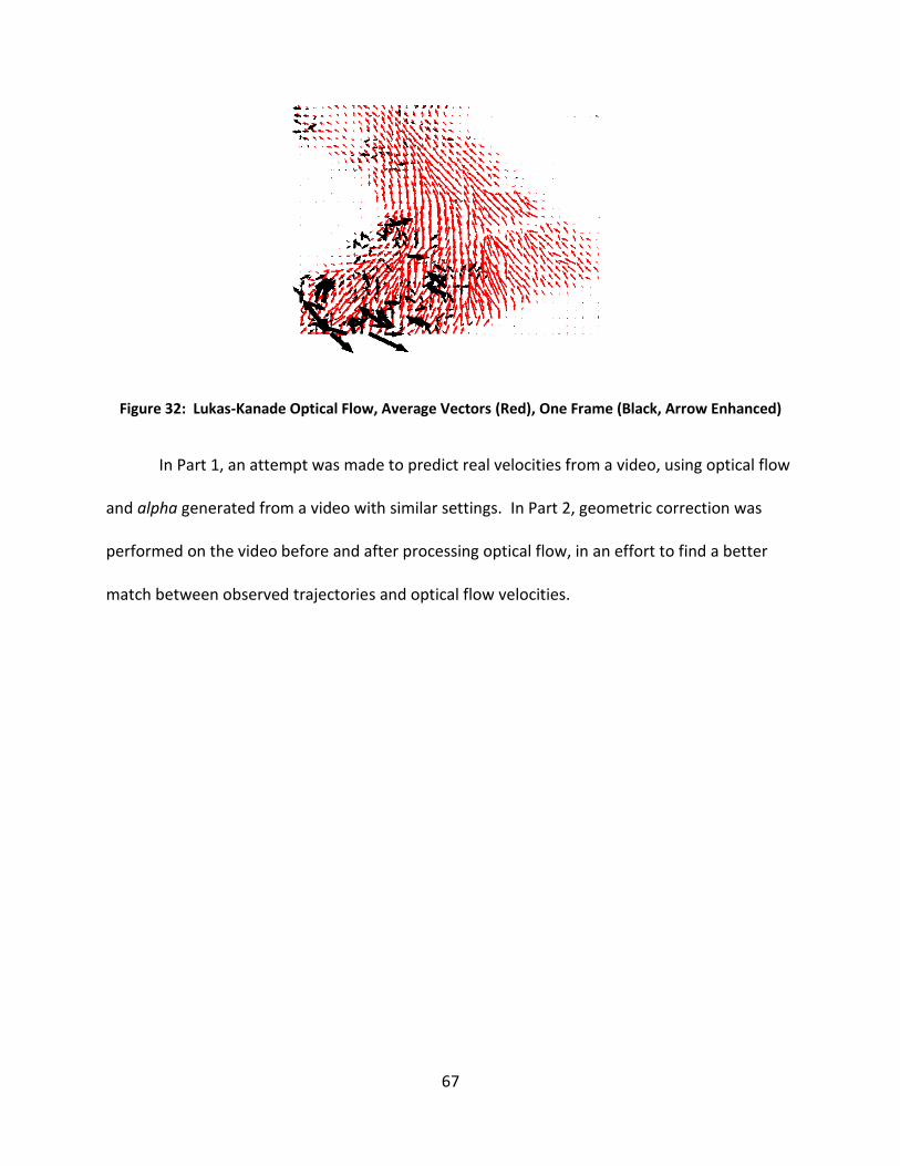
67

Figure 32: Lukas-Kanade Optical Flow, Average Vectors (Red), One Frame (Black, Arrow Enhanced)

In Part 1, an attempt was made to predict real velocities from a video, using optical flow

and alpha generated from a video with similar settings. In Part 2, geometric correction was

performed on the video before and after processing optical flow, in an effort to find a better

match between observed trajectories and optical flow velocities.

68

4. PART 2: EXPERIMENTS USING SIMULATION VIDEOS

4.1 Methods

In Part 2, the video of a simulation was treated in two ways: (1) correcting the

geometric distorts in the video and then running optical flow, and (2) running optical flow on

the uncorrected video and then geometrically correcting the output data. The results of each

process were compared to the actual velocities to see which process produced a better

correlation. They were also compared to the optical flow of the actual velocities. Figure 33

shows the process flow chart.

PIV optical

flow

NetLogo3-D NetLogo

video

Geometric

correction

Geometric

correcion

PIV optical

Flow

CP Process

PCI Process

Compare to

1. NetLogo track

2. NetLogo PIV

Interpolation

Part 2

Figure 33: Flow Chart of the Process Used in Part 2

69

4.1.1 Simulation Experiments

Simple simulations were created using NetLogo software. “NetLogo is a multi-agent

programmable modeling environment” that comes with a large library of models, and can be

downloaded free of charge (Wilensky, 1999). The graphical display, which is the NetLogo

coordinate plane, has a background consisting of patches. Patch size and color can be varied.

The agents are called turtles. Turtles can have different shapes, sizes and colors. They can

move with a predetermined, variable step size, but here we only used a fixed step size.

NetLogo keeps track of all turtle positions – an output similar to manual tracking performed on

real videos – from which velocities and directions can be calculated. Turtle behavior can also be

programmed, but we only studied the case where all turtles moved at the same constant

velocity. Particle Image Velocimetry was used to study videos of the simulations created in

NetLogo.

For this experiment, a NetLogo patch was 4x4 pixels. Turtles’ shapes were chosen to be

circles. They were given random colors. The background was sky color. The ground was

divided into areas with motion in the positive vertical direction (up) and areas with motion in

the negative vertical direction (down). A grid drawn on the NetLogo background helped to

calibrate the model; later it was removed as it hindered PIV. Other research in the SimMBioS

project deals with background removal. Videos were created by capturing one image every

time the turtles made one step each. Step size was varied to study different velocities. For this

experiment, all turtles were moving at the same predetermined speed. The number of turtles

on the NetLogo ground can be determined, but not in the cropped and geometrically corrected

70

frames (unless manually counted). Therefore, the generation rate of new turtles was used as a

parameter instead.

4.1.1.1 Simulation Videos

The simulations consisted of a background where turtles were moving only in the

vertical direction. The ground was divided into four quarters, with turtles moving in opposite

directions in adjacent quarters. Directions of movement are shown in the PIV result in Figure

34, where the velocity of each of the colors (red, green and blue) is shown by a corresponding

colored arrow. The arrows are at the centers of 40x40 pixels cells. Three parameters were

varied and optical flow of the resulting videos studied. The three parameters were: size of

turtle, or diameter, spatial step size, which determines velocity, and generation rate, which

determines the number of turtles present in the experiment. Images were captured after every

step, and PIV was calculated for every pair of frames; so there was an optical flow velocity in

each cell for every step.

The ground can be seen as a two-dimensional (2-D) plan or bird’s eye view (what is

herein called “model view”), as well as a three-dimensional (3-D) view at any angle and from

any height (what is herein called the “screen view”). These two views are shown in Figure 35.

The grid is drawn so that the resulting squares on the model view are cells of 40x40 pixels.

Using a NetLogo program that Dr. Thomas Clarke created, the simulation video of either the

model view or the screen view could be recorded. The NetLogo program also keeps record of

the positions of turtles at every time step in the NetLogo coordinate plane, from which track

velocities can be calculated.

71

Figure 34: Velocity of Turtles (Colored Arrows)

To facilitate the calibration of geometric transforms, grid lines were programmed into

the background of the NetLogo simulations. The exact location of the grid intersections on the

screen view (the 3-D view) were used only to obtain a transformation matrix that transforms

positions from screen view, to either ground or model view. Background gridlines were later

removed, and a sky color was used for the entire background. The experiments did not have

gridlines, as the stationary background interferes with optical flow results.

72

Figure 35: NetLogo Set-Up Showing the 2-D Model View and the 3-D Perspective View

The next step was to obtain a video in a suitable format. The gray square in Figure 35

was composed of 109x109 NetLogo ground patches, of patch size 4x4 pixels. This produced

videos of 436x436 pixels. The 3-D video was then cropped to a workable area, with a frame

size of 320 x 240 (Figure 36). This became our screen view. This video was then used in the

two processes of Part 2. Outputs from the two routes were later compared to the original

NetLogo turtle velocities. This comparison was done twice: once using the real tracked

positions of each turtle, from which their velocity was calculated. In the second comparison,

PIV from the 2-D NetLogo model view was compared to PIV obtained from the two procedures

that included the geometric transformation. Subsequently, an evaluation was performed to

compare the two methods.

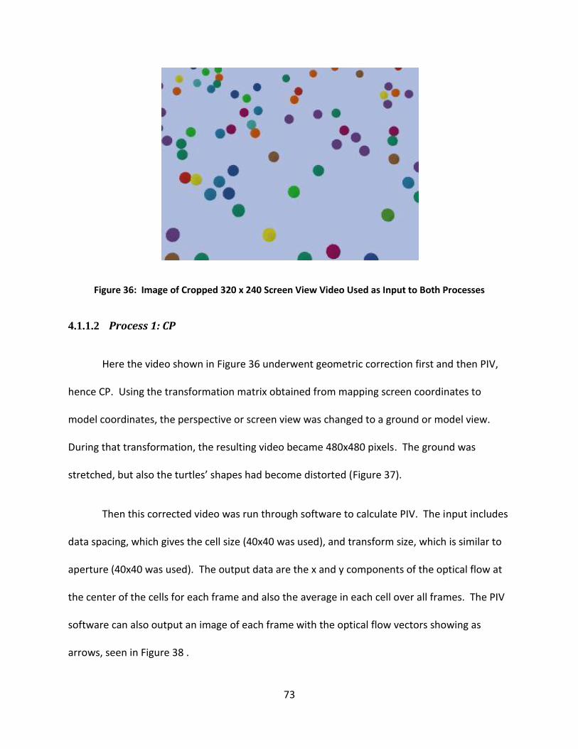
73

Figure 36: Image of Cropped 320 x 240 Screen View Video Used as Input to Both Processes

4.1.1.2 Process 1: CP

Here the video shown in Figure 36 underwent geometric correction first and then PIV,

hence CP. Using the transformation matrix obtained from mapping screen coordinates to

model coordinates, the perspective or screen view was changed to a ground or model view.

During that transformation, the resulting video became 480x480 pixels. The ground was

stretched, but also the turtles’ shapes had become distorted (Figure 37).

Then this corrected video was run through software to calculate PIV. The input includes

data spacing, which gives the cell size (40x40 was used), and transform size, which is similar to

aperture (40x40 was used). The output data are the x and y components of the optical flow at

the center of the cells for each frame and also the average in each cell over all frames. The PIV

software can also output an image of each frame with the optical flow vectors showing as

arrows, seen in Figure 38 .

74

Figure 37: Image of Geometrically Corrected Video

Figure 38: Image of Geometrically Corrected Frame with PIV Vectors, a Step in the CP Process

75

4.1.1.3 Process 2: PCI

Here optical flow of the video of Figure 36 was acquired first. The resulting video image

and the PIV result are shown in Figure 39.

Figure 39: Cropped Video from Figure 36, after being processed by the PIV Optical Flow, an Intermediate Step in the PCI Process

The data obtained are velocity components located at the center of 40x40 cells on this

320 x 240 pixel frame. Then, first the positions were transformed using the equations shown

later in section ‎4.1.3.2, and subsequently a different transform was used for velocities, as

76

described in ‎4.1.3.3. Finally, as the transformed positions were located in a pattern as shown in

Figure 40a, velocities not only had to be transformed, but interpolation was done to get their

values at the positions in Figure 40b, in order to compare them to the data from the CP process.

a. Positions after Geometric Transformation b. Positions Needed for Comparisons

Figure 40: Velocity Positions

4.1.2 Beta Approximation

Drawing an analogy between linear (scalar) and vector correlation, the best fit line is

and the slope of the line is

(Hanson, et al., 1992) .

is a complex expression. When there is no movement, both optical flow and observed

velocities should be zero. Thus the intercept is expected to be zero and was so taken to be.

Therefore, using the concept of least squares, we would like to see the sum of the squares of

the error to be a minimum. The regression coefficient between

vectors z and w that minimizes then is

0

50

100

150

200

250

300

350

400

450

500

0 200 400

0

50

100

150

200

250

300

350

400

450

500

0 200 400

77

( 5 )

where

and

and

4.1.3 Geometric Correction

In general, optical flow works best with bird’s eye view images (seen from top down). It

is difficult to position cameras to obtain such images in an urban setting, however, for example

in a train station. Distortion arises from the positioning of the video camera and from the lens

curvature. The simulation video underwent geometric correction as if we did not know the

camera properties and position and was done instead from knowledge of the positions of key

objects in the video.

To transform from the screen view to the model view, the perspective transformation is

needed. The perspective transformation matrix that relates screen coordinates to model

coordinates is normally given in terms of the camera parameters, such as camera location,

orientation and focal length, which are frequently not known. Since the camera parameters

may not be known, Excel was used to calculate the matrix that gives the best transformation. If

the coordinates of a few points (four or more) on the ground, and their corresponding pixel

coordinates on the frame, are known, then the required matrix can be acquired. The input to

our transformation software, written in Microsoft Excel, includes true model (ground)

78

coordinates, screen coordinates and some parameters related to the size of the frame. Excel

Solver can then calculate the components of the transformation matrix, by minimizing the

square of the error between the given model coordinates and the corresponding transformed

screen coordinates.

4.1.3.1 Transformation Matrices

In a geometric transformation, we start with translation, rotation, and/or scaling of the

real ground to coincide with vertical and horizontal x-y coordinates, as shown in Figure 41. The

resulting 2-D ground, coordinates will be referred to as model coordinates (xm, ym).

The video frames, which are equivalent to a 3-D view, will herein be referred to as

screen view, and will have coordinates (xs, ys). A transformation matrix (T) takes screen

coordinates and transforms them into model coordinates. An example is shown in Figure 42,

where the video image (top) was first cropped to the desired area, middle. The new video was

then transformed to model view (bottom), using a transformation matrix. The top of the frame

is stretched more than the bottom in both the x and y directions.

z

Figure 41: Change of Ground Coordinates to Model Coordinates

Ground Model

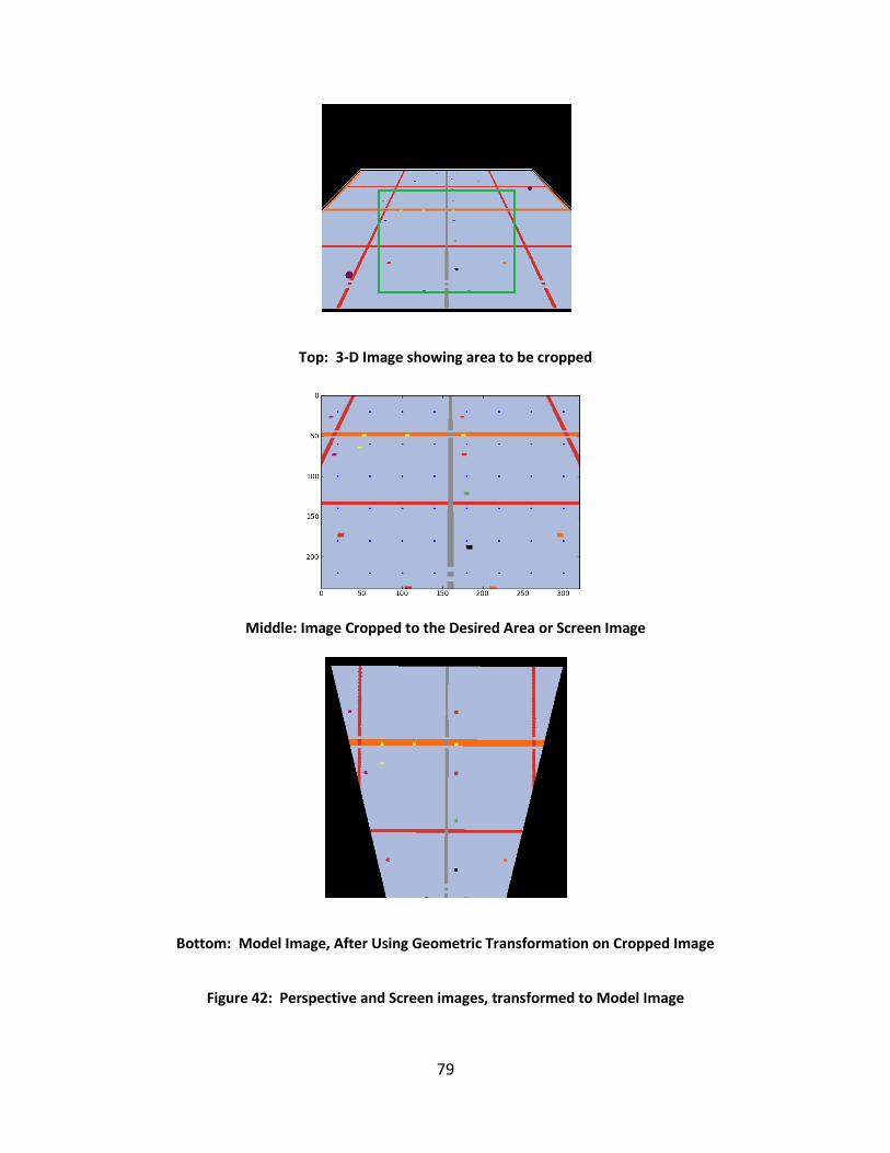
79

Top: 3-D Image showing area to be cropped

Middle: Image Cropped to the Desired Area or Screen Image

Bottom: Model Image, After Using Geometric Transformation on Cropped Image

Figure 42: Perspective and Screen images, transformed to Model Image

80

The transformation occurs when:

where um is a scaling factor and the transformation matrix T is

To obtain the transformation matrix needed for the NetLogo simulation experiment, the

background of the experiment was drawn with gridlines. The coordinates of the grid

intersections on the NetLogo 2-D ground (model) (xm, ym) and on the corresponding 3-D frames

(screen), (xs, ys), were recorded. A scaling factor was calculated using the screen sizes. A

transformation matrix was found by comparing the calculated (xm, ym) coordinates to the pre-

set NetLogo coordinates, and minimizing the error between them with Excel Solver. The

resulting transformation matrix was used to calculate positions, as well as to transform

velocities.

The transformation matrix was used in both processes. In the CP process it changes the

video screen view to model view. In the PCI process, it was used twice, once to change the

positions of screen optical flow to model positions, and another to recalculate velocities. The

model positions, which are the transformed centers of the cells drawn on the perspective

screen view, are generally not in the center of the rectangular cells drawn on the model view,

and the resulting transformed velocities were also not located on a rectangular grid, as seen in

81

Figure 40a. Therefore, the velocities had to be interpolated into the values they would have on

a rectangular grid as shown in the right diagram of Figure 40b.

4.1.3.2 Transforming Positions

In the CP process, pixel positions of the 3-D video were transformed using the

transformation matrix, thus producing a second video. This new video had vertical and

horizontal grids corresponding to (xm, ym), before running optical flow software. In the PCI

process, optical flow was run on the perspective screen images. The resulting PIV velocities

were located at the centers of cells drawn on the screen image. After geometric

transformation of the ground, as the screen was stretched, the positions were no longer on a

rectangular grid (in the center of the cells), as seen in the left diagram of Figure 40a, For

example, position (20, 20) on the screen of the NetLogo experiment corresponded to (9.6, 7.3)

on the 2-D model ground.

To get (xm, ym) from the screen coordinates (xs, ys), the following transformation was

used:

(2)

82

4.1.3.3 Transforming Velocities

Dr. Clarke calculates the transformed velocities in an unpublished paper (Clarke, 2009)

as follows:

(3)

where

are the velocities on the screen, to be precise, the PIV velocities obtained

from the perspective 3-D video. These velocities were transformed to model velocities located

at points that do not correspond to intersections of a rectangular grid. To be able to compare

them to other optical flow and actual track velocities, they needed to be interpolated to the

centers of cells that are analogous to other experiments. The interpolation was performed

using a Microsoft Excel Add-in called Xongrid ("XonGrid," 2010). It interpolates using the

Kriging method. Given the values of at several points (x, y), and the coordinates of a specific

point (x0, y0), this method uses weighting and a linear least squares calculation that results in

the interpolated value of Vx at the new point (x0, y0).

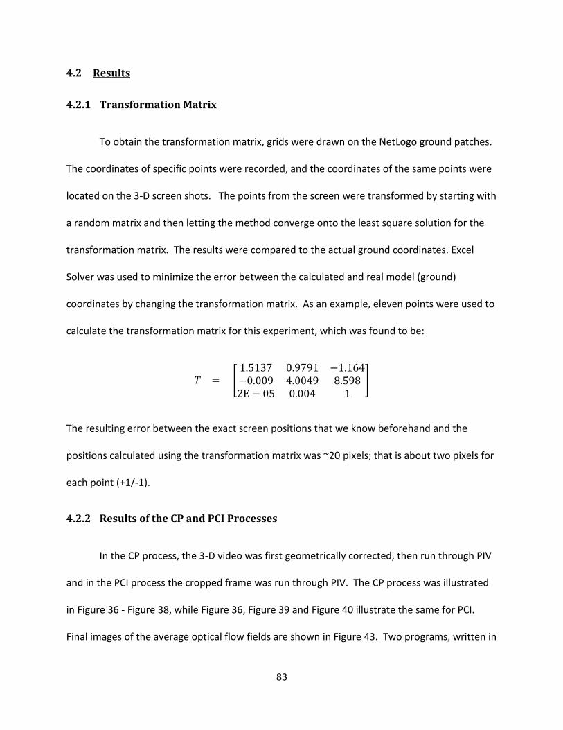
83

4.2 Results

4.2.1 Transformation Matrix

To obtain the transformation matrix, grids were drawn on the NetLogo ground patches.

The coordinates of specific points were recorded, and the coordinates of the same points were

located on the 3-D screen shots. The points from the screen were transformed by starting with

a random matrix and then letting the method converge onto the least square solution for the

transformation matrix. The results were compared to the actual ground coordinates. Excel

Solver was used to minimize the error between the calculated and real model (ground)

coordinates by changing the transformation matrix. As an example, eleven points were used to

calculate the transformation matrix for this experiment, which was found to be:

The resulting error between the exact screen positions that we know beforehand and the

positions calculated using the transformation matrix was ~20 pixels; that is about two pixels for

each point (+1/-1).

4.2.2 Results of the CP and PCI Processes

In the CP process, the 3-D video was first geometrically corrected, then run through PIV

and in the PCI process the cropped frame was run through PIV. The CP process was illustrated

in Figure 36 - Figure 38, while Figure 36, Figure 39 and Figure 40 illustrate the same for PCI.

Final images of the average optical flow fields are shown in Figure 43. Two programs, written in

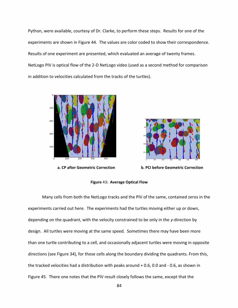
84

Python, were available, courtesy of Dr. Clarke, to perform these steps. Results for one of the

experiments are shown in Figure 44. The values are color coded to show their correspondence.

Results of one experiment are presented, which evaluated an average of twenty frames.

NetLogo PIV is optical flow of the 2-D NetLogo video (used as a second method for comparison

in addition to velocities calculated from the tracks of the turtles).

a. CP after Geometric Correction b. PCI before Geometric Correction

Figure 43: Average Optical Flow

Many cells from both the NetLogo tracks and the PIV of the same, contained zeros in the

experiments carried out here. The experiments had the turtles moving either up or down,

depending on the quadrant, with the velocity constrained to be only in the y-direction by

design. All turtles were moving at the same speed. Sometimes there may have been more

than one turtle contributing to a cell, and occasionally adjacent turtles were moving in opposite

directions (see Figure 34), for those cells along the boundary dividing the quadrants. From this,

the tracked velocities had a distribution with peaks around + 0.6, 0.0 and - 0.6, as shown in

Figure 45. There one notes that the PIV result closely follows the same, except that the

85

nonzero peaks are more delocalized and some from the zero peaks have taken on nonzero

values. Figure 46 shows similar histograms after the data has been processed by the CP and PCI

processes. The data from the CPI process clearly has had some of the original zero cells moved

to nonzero values with the original two distinct peaks becoming more spread out The loss of

zero cells is probably more due to the interpolation, as the linear interpolation was calculated

from several surrounding points, a weighted average in effect. .

NetLogo Tracks - Vy

CP- Vy

PCI- Vy

NetLogo PIV,- Vy

Red is a lower/negative number, green is higher number

Figure 44: Vy of Average of 20 frames; NetLogo Tracks, CP-PIV and PCI-PIV

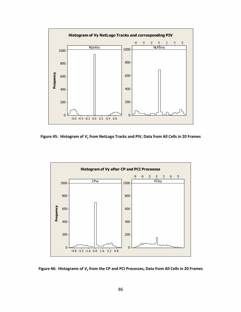
86

0.60.40.20.0-0.2-0.4-0.6

1000

800

600

400

200

0

6420-2-4-6

1000

800

600

400

200

0

NLtrkVy

Fre

qu

en

cy

NLPIVvy

Histogram of Vy NetLogo Tracks and corresponding PIV

Figure 45: Histogram of Vy from NetLogo Tracks and PIV, Data from All Cells in 20 Frames

4.83.21.60.0-1.6-3.2-4.8

1000

800

600

400

200

0

9630-3-6-9

1000

800

600

400

200

0

CPvy

Fre

qu

en

cy

PCIvy

Histogram of Vy after CP and PCI Processes

Figure 46: Histograms of Vy from the CP and PCI Processes, Data from All Cells in 20 Frames

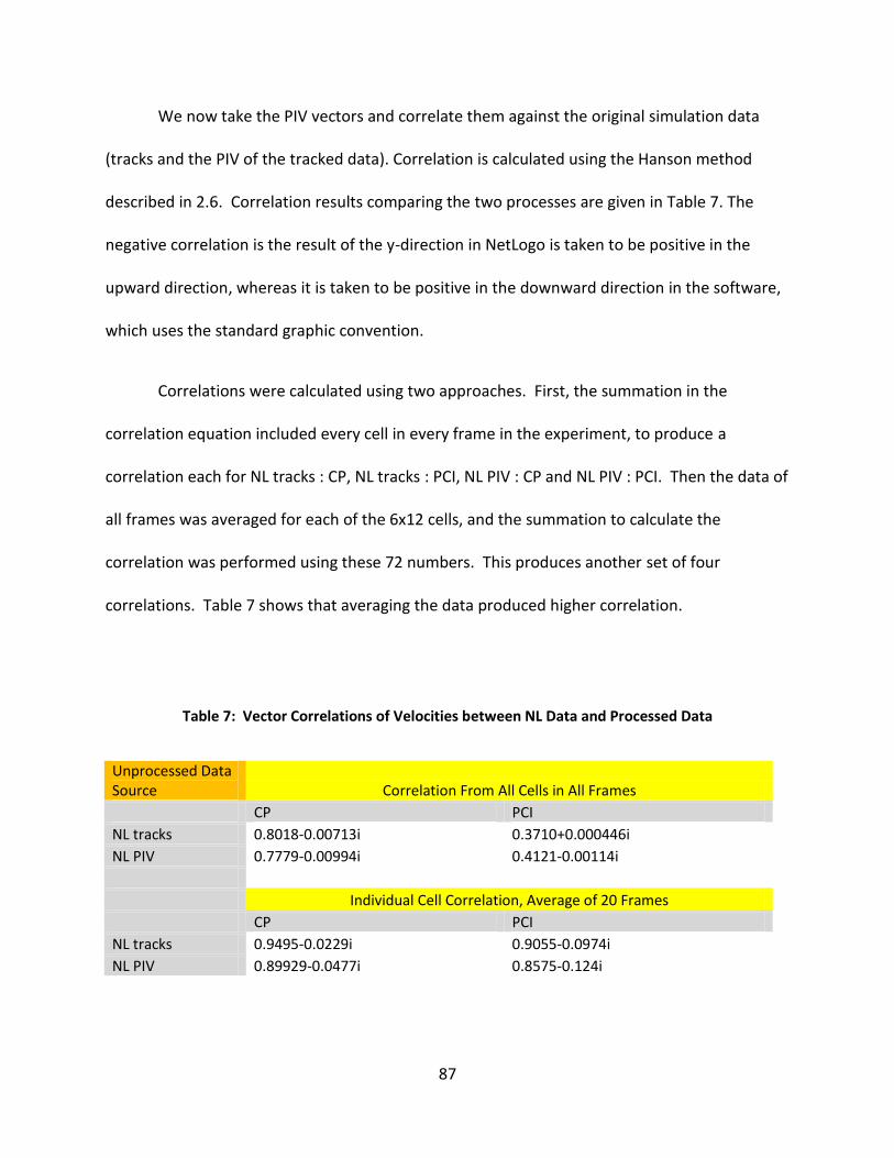
87

We now take the PIV vectors and correlate them against the original simulation data

(tracks and the PIV of the tracked data). Correlation is calculated using the Hanson method

described in ‎2.6. Correlation results comparing the two processes are given in Table 7. The

negative correlation is the result of the y-direction in NetLogo is taken to be positive in the

upward direction, whereas it is taken to be positive in the downward direction in the software,

which uses the standard graphic convention.

Correlations were calculated using two approaches. First, the summation in the

correlation equation included every cell in every frame in the experiment, to produce a

correlation each for NL tracks : CP, NL tracks : PCI, NL PIV : CP and NL PIV : PCI. Then the data of

all frames was averaged for each of the 6x12 cells, and the summation to calculate the

correlation was performed using these 72 numbers. This produces another set of four

correlations. Table 7 shows that averaging the data produced higher correlation.

Table 7: Vector Correlations of Velocities between NL Data and Processed Data

Unprocessed Data Source Correlation From All Cells in All Frames

CP PCI

NL tracks 0.8018-0.00713i 0.3710+0.000446i

NL PIV 0.7779-0.00994i 0.4121-0.00114i

Individual Cell Correlation, Average of 20 Frames

CP PCI

NL tracks 0.9495-0.0229i 0.9055-0.0974i

NL PIV 0.89929-0.0477i 0.8575-0.124i

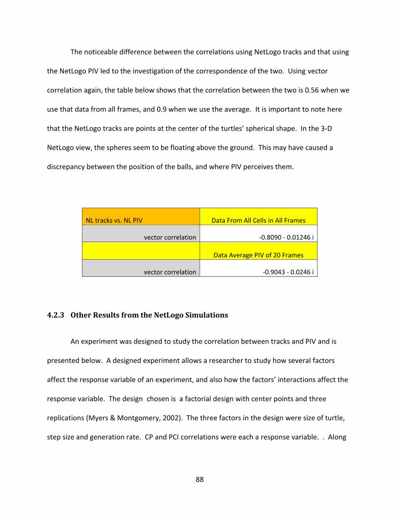
88

The noticeable difference between the correlations using NetLogo tracks and that using

the NetLogo PIV led to the investigation of the correspondence of the two. Using vector

correlation again, the table below shows that the correlation between the two is 0.56 when we

use that data from all frames, and 0.9 when we use the average. It is important to note here

that the NetLogo tracks are points at the center of the turtles’ spherical shape. In the 3-D

NetLogo view, the spheres seem to be floating above the ground. This may have caused a

discrepancy between the position of the balls, and where PIV perceives them.

NL tracks vs. NL PIV Data From All Cells in All Frames

vector correlation -0.8090 - 0.01246 i

Data Average PIV of 20 Frames

vector correlation -0.9043 - 0.0246 i

4.2.3 Other Results from the NetLogo Simulations

An experiment was designed to study the correlation between tracks and PIV and is

presented below. A designed experiment allows a researcher to study how several factors

affect the response variable of an experiment, and also how the factors’ interactions affect the

response variable. The design chosen is a factorial design with center points and three

replications (Myers & Montgomery, 2002). The three factors in the design were size of turtle,

step size and generation rate. CP and PCI correlations were each a response variable. . Along

89

with the optical flow study, other results were found related to the designed experiment which

we shall now describe.

Pareto charts, for the three factors and their interactions are shown in Figure 47. These

bar graphs indicate the importance or non-importance of any factor on the prediction of a

response. The effect of a factor on shifting the value of the response variable from an expected

value is represented by a column. The red line denotes the value that the effect has to reach to

become statistically significant ("Minitab Statistical Software," 2007). The diagrams show that

for the CP process, only the generation rate of turtles, which is an indication of number of

turtles in the experiment, significantly contributes to the variation in the CP correlation; none

of the three factors was a determining factor in the correlation in the PCI experiment.

Contour plots are shown below in Figure 48. The colors show the degree of correlation

in the CP experiments, blue being higher. Figure 48 and Figure 49 indicate that the highest

correlation occurs at a turtle size somewhere between the two sizes chosen (5 and 20). A

greater generation rate leads to higher correlations, and at the smaller step size. Figure 50

confirms these results.

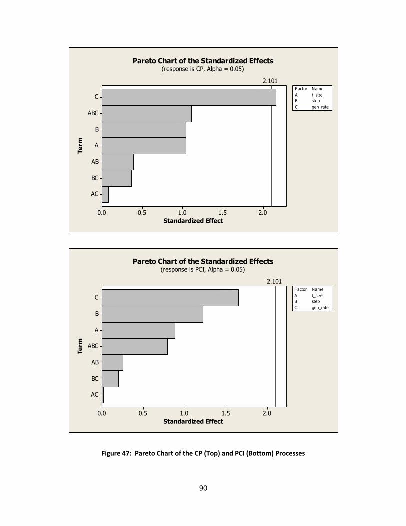
90

AC

BC

AB

A

B

ABC

C

2.01.51.00.50.0

Te

rm

Standardized Effect

2.101

A t_size

B step

C gen_rate

Factor Name

Pareto Chart of the Standardized Effects(response is CP, Alpha = 0.05)

AC

BC

AB

ABC

A

B

C

2.01.51.00.50.0

Te

rm

Standardized Effect

2.101

A t_size

B step

C gen_rate

Factor Name

Pareto Chart of the Standardized Effects(response is PCI, Alpha = 0.05)

Figure 47: Pareto Chart of the CP (Top) and PCI (Bottom) Processes

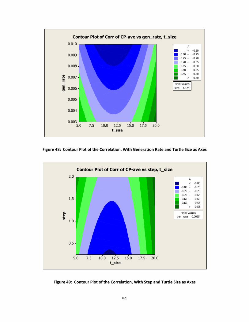
91

t_size

ge

n_

rate

20.017.515.012.510.07.55.0

0.010

0.009

0.008

0.007

0.006

0.005

0.004

0.003

step 1.125

Hold Values

>

–

–

–

–

–

–

< -0.80

-0.80 -0.75

-0.75 -0.70

-0.70 -0.65

-0.65 -0.60

-0.60 -0.55

-0.55 -0.50

-0.50

A

Contour Plot of Corr of CP-ave vs gen_rate, t_size

Figure 48: Contour Plot of the Correlation, With Generation Rate and Turtle Size as Axes

t_size

ste

p

20.017.515.012.510.07.55.0

2.0

1.5

1.0

0.5

gen_rate 0.0065

Hold Values

>

–

–

–

–

–

< -0.80

-0.80 -0.75

-0.75 -0.70

-0.70 -0.65

-0.65 -0.60

-0.60 -0.55

-0.55

A

Contour Plot of Corr of CP-ave vs step, t_size

Figure 49: Contour Plot of the Correlation, With Step and Turtle Size as Axes

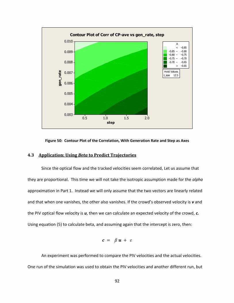
92

step

ge

n_

rate

2.01.51.00.5

0.010

0.009

0.008

0.007

0.006

0.005

0.004

0.003

t_size 12.5

Hold Values

>

–

–

–

–

< -0.85

-0.85 -0.80

-0.80 -0.75

-0.75 -0.70

-0.70 -0.65

-0.65

A

Contour Plot of Corr of CP-ave vs gen_rate, step

Figure 50: Contour Plot of the Correlation, With Generation Rate and Step as Axes

4.3 Application: Using Beta to Predict Trajectories

Since the optical flow and the tracked velocities seem correlated, Let us assume that

they are proportional. This time we will not take the isotropic assumption made for the alpha

approximation in Part 1. Instead we will only assume that the two vectors are linearly related

and that when one vanishes, the other also vanishes. If the crowd’s observed velocity is v and

the PIV optical flow velocity is u, then we can calculate an expected velocity of the crowd, c.

Using equation (5) to calculate beta, and assuming again that the intercept is zero, then:

An experiment was performed to compare the PIV velocities and the actual velocities.

One run of the simulation was used to obtain the PIV velocities and another different run, but

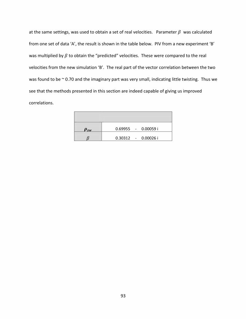
93

at the same settings, was used to obtain a set of real velocities. Parameter was calculated

from one set of data ‘A’, the result is shown in the table below. PIV from a new experiment ‘B’

was multiplied by to obtain the “predicted” velocities. These were compared to the real

velocities from the new simulation ‘B’. The real part of the vector correlation between the two

was found to be ~ 0.70 and the imaginary part was very small, indicating little twisting. Thus we

see that the methods presented in this section are indeed capable of giving us improved

correlations.

0.69955 - 0.00059 i

0.30312 - 0.00026 i

94

5. DISCUSSION AND CONCLUSIONS

Results above have shown that the attempt at lowering the variation in alpha had a

modest effect. Therefore, an attempt was made to study what was impeding the

improvement. This approach required that the background and motion be controlled. The

open source software NetLogo was used. Through NetLogo, the background color can be

manipulated, as well as the shape, size and color.

5.1 Sources of Error

5.1.1 Stationary Background

The major source of error noticed was the existence of stationary background objects in

the videos. When the NetLogo experiments were carried out, they were first tried with a grid

on the ground to facilitate calibration. Figure 51 shows the optical flow vectors of turtles

moving on a gridded background. The vectors are very small, almost non-existent. Optical Flow

attempts to find a region in the second frame where the light intensity has the highest

correlation with a region in the first frame. The moving turtle may not be the determining

factor. The stationary grid has a great influence, especially if only a small part of the turtle is in

the cell, and the rest of the pixels are background. Optical flow then finds the best correlation

is to fit the background rather than the moving turtle. The figure also shows that some of the

turtles do not have visible arrows associated with them. In contrast, the same turtles moving at

the same step size on a plain background have larger vectors associated with them, Figure 52.

95

Figure 51: PIV Optical Flow Vectors of Turtles Moving on a Gridded Background

Figure 52: PIV Optical Flow Vectors of Turtles Moving on a Plain Background

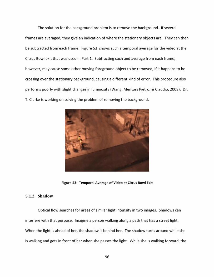
96

The solution for the background problem is to remove the background. If several

frames are averaged, they give an indication of where the stationary objects are. They can then

be subtracted from each frame. Figure 53 shows such a temporal average for the video at the

Citrus Bowl exit that was used in Part 1. Subtracting such and average from each frame,

however, may cause some other moving foreground object to be removed, if it happens to be

crossing over the stationary background, causing a different kind of error. This procedure also

performs poorly with slight changes in luminosity (Wang, Mentors Pietro, & Claudio, 2008). Dr.

T. Clarke is working on solving the problem of removing the background.

Figure 53: Temporal Average of Video at Citrus Bowl Exit

5.1.2 Shadow

Optical flow searches for areas of similar light intensity in two images. Shadows can

interfere with that purpose. Imagine a person walking along a path that has a street light.

When the light is ahead of her, the shadow is behind her. The shadow turns around while she

is walking and gets in front of her when she passes the light. While she is walking forward, the

97

shadow is moving in several directions. When optical flow is detecting where there is

movement in this part of the frame, there is confusion. The Citrus Bowl video used for alpha

calculations was a night-time video, and this was one of the reasons for poor results. Computer

vision research that is associated with surveillance and traffic monitoring explores this subject

(Cucchiara, Grana, Piccardi, & Prati, 2003; Sheng, Dequn, Xiaoyan, & Qiang, 2007; Shoaib,

Dragon, & Ostermann, 2009).

5.1.3 Color and Contrast

The Lukas-Kanade based software used here operates on monochrome images and can

handle different levels of contrast. The Particle Image Velocimetry software was set up to

handle the three RBG colors separately. Andrews, et al. (2003) state that the computation

using color gives the same level of accuracy as grayscale, and reduces the amount of

computation. In general, colors can give additional useful information. The effect of color was

not studied in this research.

5.1.4 Geometry

A transformation matrix to correct for the perspective view deforms both the

background and the foreground, if the heights of objects in them are not uniform. An attempt

to transform the Citrus Bowl images into ground rectangular coordinates resulted in Figure 54.

The ground is basically rectangular, but as one can see, the vertical lines do not seem vertical.

The people in the image appear stretched, and we cannot see them from a bird’s eye view.

That will be a source of error in optical flow results, when attempting to compare geometrically

corrected video to the ground view (model view) of a simulation or to observed tracks.

98

Figure 54: Citrus Bowl Exit Image after Geometric Transformation

In the NetLogo simulations there was a similar difficulty. The shape chosen for the

turtles was a ball. In the 3-D view, the balls seem to be floating above the ground. In our

geometric transformation, we only dealt with the x and y directions on the ground and ignored

the height in the z direction. In the future, the elevation of the shapes should be taken into

account when correcting the video.

As seen in Figure 36 and Figure 37, geometric transformation of the ground results in

geometric transformation of the NetLogo turtles also. Ideally, geometric transformation should

return the screen view turtle to a ground view turtle, but this does not happen experimentally.

Optical flow reads the displacement of the blobs of various light intensities, which is essentially

the area of the turtle. A larger turtle or blob area (or number of pixels) moving result in

different values for optical flow. The effect of the shape was not investigated.

5.1.5 Direction of Motion, Crowd Density and Flow

Optical Flow in cells, as applied in these experiments, averages the motion of many

pixels into a value for one vector at the center of the cell. For this description to be accurate,

99

the motion of all the pixels in the cell would ideally be in the same direction, and at the same

speed. Cells that are too large may include areas where there is no motion, or where there is

motion not in the same direction. If the flow of the crowd is steady like a stream, and we are

averaging several frames, then optical flow can still detect an odd motion of people slowing

down around a person that falls. If we use small enough cells, we may be able to detect

someone walking against the flow. However, when the scene is sparse to start with, this is a

cause of errors.

5.2 Conclusion

The objective of this thesis was to find a method to validate optical flow, so that optical

flow can be compared to observed track velocities of individuals in a way that will prove their

correspondence, with the intention that optical flow can in turn be used to validate simulations.

In Part 1, the best conditions that would result in a measurable proportionality relation alpha

between optical flow and observed tracks were sought. Towards that purpose, several

experiments were performed and parameters varied to find conditions where alpha would hold

to be a reasonable measure of proportionality, with a low coefficient of variation. The

coefficient of variation of alpha fluctuated, sometimes even up to ninety percent.

The coefficient of variation of alpha was found to be lower when larger apertures were

used (‎3.2.1.2). Optical flow searches in frame n+1 around a pixel for the best possible

correlation to the light intensity pattern found in frame n. The wider aperture allows added

opportunity to find the right pattern. This may imply that the steps (distances) of the motion

were larger than the small apertures of 15x15 allowed by the Lukas-Kanade method. In the

100

future, every frame should be used instead of every 5th frame to obtain smaller steps. PIV, in

contrast, can be set to an aperture of 40x40, and could be used for faster motion or larger

steps.

Alpha varied less with smaller optical flow thresholds in the video under investigation

(‎3.2.1.1). This indicates that, in this case, more details in the image supply better information

and thus lead to better results. Other videos may be different. In contrast, alpha varied less

when the optical flow velocities were averaged into larger cells (‎3.2.3.1). This averaging

smoothed the variation, even though it caused loss of detail. The detail level required for a

specific experiment will decide what size of a cell to use.

Averaging a few frames together worked better for my experiments. The video was

sparse at times, with many cells having no motion in them. Averaging then brings values other

than zero to some of the cells in the path of the crowd, thus giving larger fluctuations to the

flow. Averaging frames also gives a better indication of the flow rather than the individual or

instantaneous velocities at the time the video frame was shot. If the aim is to compare the flow

in general, then averaging several frames is the way to proceed, provided the flow does not

change significantly over the period of the averaging.

Smoothing the manually tracked paths data by spreading the velocity position from one

pixel into a rectangle improved the correlation between optical flow and observed tracks. (See

section 3.2.2.2) Optical flow in a cell takes into account all pixels that have a velocity

associated with them, and should be compared to a similar moving area rather than one pixel

moving. It could be possible to vary the size of the rectangle, depending on the position in the

101

frame, in an effort to match the size of a person and partially solve the perspective issue. This

is expected to further improve correlations, and hence the variation in alpha.

Segmenting out the cells with the most flow did not reduce alpha’s variation (‎3.2.3.4),

nor did excluding the cells that hardly had any moving crowd in them (‎3.2.3.3). The results of

these experiments may have been deceiving, however. The variation in alpha could have been

lower because of the existence of many cells with very low optical flow and zero tracked

motion. The many zeros could have had good correlations that reduced alpha variation.

Frames with no motion are expected to give good correspondence. The use of chosen center

cells may be justified depending on the requirements of the experiment.

Alpha was used to predict tracks. Comparing the predicted velocities with the actual

observed ones, when alpha frame was used in the prediction, the vector correlation of 100

frame segments was found to be 0.25-0.29 (‎3.3.1). Combining data from all frames, using an

alpha calculated for each cell resulted in a correlation of about 0.7, which was better than using

alpha row or alpha frame (‎3.3.3). Having a different alpha for every cell takes into account the

areas with consistent crowd flow and those with no flow. It also takes into account the position

on the screen, which is related to the perspective view.

Of the two processes that were presented in Part 2 of the thesis, the CP process where

geometric correction of the perspective was completed first, followed by optical flow, gave

better correlations than using the PCI process, where optical flow was run first, and then the

velocity values corrected (‎4.2.2). CP is also the faster of the two processes. The foreground,

however, gets distorted when the geometric correction of the ground is performed. Still, CP

102

proved to be the better process. Continuing with these NetLogo experiments, different camera

positions can be investigated to find the effect of camera height. Also the effect of background

and turtle color can be studied.

Using tracked positions to calculate velocities for comparison to the output of the CP

and PCI processes was better than using PIV of the ground scene (‎4.2.2). This is a good thing.

In experiments using real crowd videos, we can get people’s positions by manual tracking and

then use those combined with geometric correction to get velocities. It normally would not be

realistic to obtain a bird’s eye view video for use to get PIV of velocities in cells.

A complex number beta was defined in section ‎4.1.2 as a proportionality parameter

between optical flow and tracks in the simulation experiments. It was used to predict tracks.

Using PIV optical flow from a new video, and beta calculated from a different video of the same

settings, one calculated an expected value for the tracks. The correlation between the

predicted and observed tracks was 0.7.

A stationary background interferes with optical flow (‎5.1.1). If the moving areas occupy

a small percentage of a cell, their optical flow is hardly detected, as the stationary areas

correlate better in consecutive frames. Simply subtracting the average of several frames is not

a complete solution. This is still an area requiring more research. Choosing cells of the order of

the size of the moving object may be one improvement in the process that would reduce the

effect of the background.

103

Correlation between manually tracked velocities and optical flow is higher when crowds

are moving in a definite direction and low when people are milling around and moving in

random directions (‎3.2.3.4). Therefore, whenever possible, choose the part of the setting that

has a continuous flow when researching optical flow. The alpha approximation should be

avoided in videos of sparse crowds. In some instances alpha seemed to be larger when there

were more people in a cell (‎3.2.2.1). This could be the next idea to pursue in trying to use

optical flow to calculate crowd density levels.

104

REFERENCES

Andrade, E. L., Blunsden, S., & Fisher, R. B. (2005). Characterisation of optical flow anomalies in pedestrian traffic. Paper presented at the The IEE International Symposium on Imaging for Crime Detection and Prevention.

Andrade, E. L., Blunsden, S., & Fisher, R. B. (2006). Hidden Markov Models for Optical Flow Analysis in Crowds. Paper presented at the 18th International Conference on Pattern Recognition, 2006.

Andrade, E. L., Fisher, R. B., & Blunsden, S. (2006). Detection of Emergency Events in Crowded Scenes. Paper presented at the The Institution of Engineering and Technology Conference on Crime and Security.

Andrews, R. J., Lovell, B. C., & Maeder, A. J. (2003). Color Optical Flow.

Baker, S., & Matthews, I. (2004). Lucas-Kanade 20 Years On: A Unifying Framework. International Journal of Computer Vision 56(3), 221–255.

Barron, J. L., Fleet, D. J., Beauchemin, S. S., & Burkitt, T. A. (1992, 15-18 Jun 1992). Performance of optical flow techniques. Paper presented at the Computer Vision and Pattern Recognition, 1992. Proceedings CVPR '92., 1992 IEEE Computer Society Conference on.

Barron, J. L., & Thacker, N. A. (2005). Tutorial: Computing 2D and 3D Optical Flow. Medical School, University of Manchester.

Beauchemin, S. S., & Barron, J. L. (1995). The computation of optical flow. ACM Comput. Surv., 27(3), 433-466.

Cédras, C., & Shah, M. (1995). Motion-based recognition a survey. Image and Vision Computing, 13(2), 129-155.

Chen, T.-H., & Hsu, C.-W. (2003). An automatic bi-directional passing-people counting method based on color image processing. Paper presented at the IEEE 37th Annual 2003 International Carnahan Conference on Security Technology.

Clarke, T. L. (2009). Coordinate Transforms for PIV Velocity Estsimation.

Clarke, T. L., Kaup, D. J., Malone, L. C., Oleson II, R., & Rosa, M. (2007). Crowd Model Verification Using Video Data. Paper presented at the International Mediterranean Modelling Multiconference Bergeggi, Italy.

105

crowd. (2009). Merriam-Webster Online Dictionary Retrieved October 5, 2009, from http://www.merriam-webster.com/dictionary/crowd

Cucchiara, R., Grana, C., Piccardi, M., & Prati, A. (2003). Detecting moving objects, ghosts, and shadows in video streams. Pattern Analysis and Machine Intelligence, IEEE Transactions on, 25(10), 1337-1342.

Dalal, N., Triggs, B., & Schmid, C. (2006). Human Detection Using Oriented Histograms of Flow and Appearance In A. Leonardis, H. Bischof & A. Pinz (Eds.), Computer Vision – ECCV 2006 (Vol. 3952/2006, pp. 428-441). Berlin / Heidelberg: Springer

Davies, A. C., Jia Hong, Y., & Velastin, S. A. (1995). Crowd monitoring using image processing. Electronics & Communication Engineering Journal, 7(1), 37-47.

Fazekas, S. a., & Chetverikov, D. (2005). Normal versus complete flow in dynamic texture recognition: a comparative study. Paper presented at the 4th International Workshop on Texture Analysis and Synthesis.

Gagvani, N. (2009). Challenges in Video Analytics Embedded Computer Vision (pp. 237-256). London: Springer.

Galvin, B., Mccane, B., Novins, K., Mason, D., & Mills, S. (1998). Recovering Motion Fields: An Evaluation of Eight Optical Flow Algorithms. Paper presented at the British Machine Vision Conference.

Gavrila, D. M. (1999). The Visual Analysis of Human Movement: A Survey. Computer Vision and Image Understanding, 73(1), 82-98.

Guerrero, T., Zhang, G., Huang, T.-C., & Lin, K.-P. (2004). Intrathoracic tumour motion estimation from CT imaging using the 3D optical flow method Physics in Medicine and Biology, 49(17), 15.

Gurka, R., & Liberzon, A. (2007). pypiv_traits_v0002.py (Version 3).

Hanson, B., Klink, K., Matsuura, K., Robeson, S. M., & Willmott, C. J. (1992). Vector Correlation: Review, Exposition, and Geographic Application. Annals of the Association of American Geographers, 82(1), 103 - 116.

Hoogendoorn, S. P., Daamen, W., & Bovy, P. H. L. (2004). Extracting Microscopic Pedestrian Characteristics from Video Data. Paper presented at the Transportation Research Board Retrieved from http://www.citg.tudelft.nl/live/pagina.jsp?id=ce418bda-1404-47ac-bcb3-ddbd7250efb2⟨=en&binary=/doc/TRB03h.pdf

Horn, B. K. P., & Schunck, B. G. (1980). Determining Optical Flow: Massachusetts Institute of Technology.

http://www.merriam-webster.com/dictionary/crowd

http://www.citg.tudelft.nl/live/pagina.jsp?id=ce418bda-1404-47ac-bcb3-ddbd7250efb2⟨=en&binary=/doc/TRB03h.pdf

http://www.citg.tudelft.nl/live/pagina.jsp?id=ce418bda-1404-47ac-bcb3-ddbd7250efb2⟨=en&binary=/doc/TRB03h.pdf

106

Hu, W., Tan, T., Wang, L., & Maybank, S. (2004). A survey on visual surveillance of object motion and behaviors. IEEE Transactions on Systems, Man, and Cybernetics, Part C: Applications and Reviews, 34(3), 334-352.

Inoue, H., Tachikawa, T., & Inaba, M. (1992, 12-14 May 1992). Robot vision system with a correlation chip for real-time tracking, optical flow and depth map generation. Paper presented at the Robotics and Automation, 1992. Proceedings., 1992 IEEE International Conference on.

Kaup, D. J., Clarke, T. L., Malone, L., Oleson, R., & Rosa, M. (2008, Sept. 17-19, 2008). On the use of Optical FLow to Test Crowd Simulations. Paper presented at the European Modeling and Simulation Symposium, Amantea, Italy.

Leggett, R. (2004). Real-Time Crowd Simulation: A Review. Retrieved October 1, 2009, from http://www.leggettnet.org.uk/docs/crowdsimulation.pdf

Lo, B. P. L., & Velastin, S. A. (2001). Automatic congestion detection system for underground platforms. Paper presented at the 2001 International Symposium on Intelligent Multimedia, Video and Speech Processing, Hong Kong.

Lucas, B. D., & Kanade, T. (1981). An iterative image registration technique with an application to stereo vision. Paper presented at the Imaging Understanding Workshop.

Ma, R., Li, L., Huang, W., & Tian, Q. (2004). On pixel count based crowd density estimation for visual surveillance. Paper presented at the 2004 IEEE Conference on Cybernetics and Intelligent Systems, Singapore.

Mahalingam, G., Kambhamettu, C., & Aguirre, B. (2009). Crowd Motion Analysis from Video. Paper presented at the 2009 NSF Engineering Research and Innovation Conference, Honolulu, Hawaii.

Malone, L. C., Clarke, T. L., Oleson II, R., Rosa, M., & Faulkner, J. (2007). Verification and Validation of Crowd Simulations Paper presented at the European Conference on Complex Systems 2007, Dresden, Germany.

Malone, L. C., Kaup, D. J., Oleson, R., Rosa, M., Jentsch, F., Clarke, T. L., et al. (2008, June 16-19). Validation of Crowd Simulations. Paper presented at the 2008 Summer Computer Simulation Conference (08SCSC), Edinburgh, Scotland

. Minitab Statistical Software (Version Minitab 15). (2007): Minitab, Inc.

Missaoui, R., & Palenichka, R. M. (2005). Effective image and video mining: an overview of model-based approaches. Paper presented at the 6th international workshop on Multimedia data mining: mining integrated media and complex data.

http://www.leggettnet.org.uk/docs/crowdsimulation.pdf

107

Moeslund, T. B., & Granum, E. (2001). A survey of computer vision-based human motion capture. Comput. Vis. Image Underst., 81(3), 231-268.

Moeslund, T. B., Hilton, A., & Krüger, V. (2006). A survey of advances in vision-based human motion capture and analysis. Computer Vision and Image Understanding, 104(2-3), 90-126.

Myers, R. H., & Montgomery, D. C. (2002). Response Surface Methodology: Process and Product Optimization Using Designed Experiments (2nd ed.). New York: John Wiley & Sons, Inc.

Park, H. H., Lee, H. G., Noh, S.-I., & Kim, J. (2006). An Area-Based Decision Rule for People-Counting Systems Multimedia Content Representation, Classification and Security (pp. 450-457). Berlin / Heidelberg: Springer

Quénot, G. M., Pakleza, J., & Kowalewski, T. A. (1998). Particle Image Velocimetry using Optical Flow for Image Analysis Paper presented at the 8th International Symposium on Flowvisualisation.

Reynolds, C. W. (1987). Flocks, herds and schools: A distributed behavioral model. Paper presented at the 14th annual conference on Computer graphics and interactive techniques.

Sargent, R. G. (2008). Verification and validation of simulation models. Paper presented at the 40th Conference on Winter Simulation.

Shah, M. (1997). Fundamentals of Computer Vision Available from http://www.cs.ucf.edu/courses/cap6411/book.pdf

Sheng, B., Dequn, L., Xiaoyan, S., & Qiang, W. (2007, 18-21 Aug. 2007). Human Cast Shadow Elimination Method Based on Orientation Information Measures. Paper presented at the Automation and Logistics, 2007 IEEE International Conference on.

Shoaib, M., Dragon, R., & Ostermann, J. (2009, 19-24 April 2009). Shadow detection for moving humans using gradient-based background subtraction. Paper presented at the Acoustics, Speech and Signal Processing, 2009. ICASSP 2009. IEEE International Conference on.

Teknomo, K., Takeyama, Y., & Inamura, H. (2000). Determination of Pedestrian Flow Performance Based on Video Tracking and Microscopic Simulations, Proceedings of Infrastructure Paper presented at the Infrastructure Planning Conference Ashikaga, Japan.

Teknomo, K., Takeyama, Y., & Inamura, H. (2001). Tracking System to Automate Data Collection of Microscopic Pedestrian Traffic Flow. Paper presented at the 4th Eastern Asia Society For Transportation Studies, Hanoi, Vietnam.

http://www.cs.ucf.edu/courses/cap6411/book.pdf

108

Velastin, S. A., Yin, J. H., Davies, A. C., Vicencio-Silva, M. A., Allsop, R. E., & Penn, A. (1994). Automated measurement of crowd density and motion using image processing. Paper presented at the Seventh International Conference on Road Traffic Monitoring and Control, London.

Vicencio-Silva, M. A. (1994). Vision based measurements of traffic parameters. Paper presented at the IEEE International Symposium on Industrial Electronics, Santiago.

Wang, Y., Mentors Pietro, P., & Claudio, F. (2008). Foreground-Background Segmentation of Video Sequences.

Westerweel, J. (1997). Fundamentals of digital particle image velocimetry. Meas. Sci. Technol., 8, 1379–1392.

Wilensky, U. (1999). NetLogo (Version 4.1): Center for Connected Learning and Computer-Based Modeling, Northwestern University, Evanston, IL.

XonGrid. (2010, 3/26). Rev 0.4. Retrieved 5/10, 2010, from http://xongrid.sourceforge.net/

Zhan, B., Monekosso, D., Remagnino, P., Velastin, S., & Xu, L.-Q. (2008). Crowd analysis: a survey. Machine Vision and Applications, 19(5), 345-357.

Zhan, B., Remagnino, P., Monekosso, D. N., & Velastin, S. (2009). The Analysis of Crowd Dynamics: From Observations to Modelling Computational Intelligence (pp. 441 -472). Berlin/Heidelberg: Springer

Zhang, X., & Sexton, G. (1995). Automatic pedestrian counting using image processing techniques. Electronics Letters, 31(11), 863-865.

http://xongrid.sourceforge.net/

Documents

Towards Calibration Of Optical Flow Of Crowd Videos Using