Towards a Perception Based Image EditingSystem

Reynold Bailey∗, Raquel Bujans†, and Cindy Grimm‡

Washington University in St. Louis

1 Introduction

The primary goal of this research is to develop a perception based image editing sys-tem. The input to this system will be either a rendered image, a photograph, or a highdynamic range image. We are currently developing techniques that allow the user toedit these images in a perceptually intuitive manner. Specifically we are consideringthe following image editing features:

1. Warm-cool image adjustment.

2. Intensity adjustment.

3. Contrast adjustment.

4. Detail adjustment.

The algorithms we are developing can be used either in an interactive editing systemor for automatic image adjustment.

2 Overview

Analysis of the chromatic properties of neurons in the visual system of the macaquemonkey led to the development of the DKL color model [1]. The visual system of themacaque is closely related to that of humans. As such, we have decided to use theDKL color model in our research. In Section 3 we introduce the DKL color modeland present several color space conversions involving the DKL color model. One ofthe goals of our work is to take a given image and make parts of it look more warmor cool. Using this approach, an artist could take a picture of a sunrise and “paint” itto look more like a sunset. We have developed a technique to generate tables of color

∗email:rjb1@cse.wustl.edu†email:rb3@cec.wustl.edu‡email:cmg@cse.wustl.edu

1

shifts. These tables show how a given hue looks when it is made to be “more warm” or“more cool”. This work is presented in Section 4. Another of our goals is to developtechniques to adjust the intensity of some input image. Our research in this area waspresented as a poster at SIGGRAPH 2004 [2] and is discussed in Section 5. We discussfuture directions of our work in Section 6.

3 DKL Color Model

In 1984, Derrington et al. [1] presented research in which they analysed the chromaticproperties of neurons in the visual system of the macaque. In their work, they de-veloped a color coding system which later became known as the DKL color model.Incorporated into the DKL color model is a mechanism for simulating the response ofthe eye’s cones and double opponent cells. The cones are cells that sense color. Theyonly trigger a response if enough light is present - a certain amount of light must bereflected off the objects in order for them to be perceived as being a certain color. Thereare three types of cones that are sensitive to short, medium, and long wavelengths ofvisible light. The double opponent cells, on the other hand, react when opposing colorsare placed next to each other. There are two main types of double opponent cells - ared-green type and a blue-yellow type. The red-green type fires a response when theeyes see a red color surrounded by a green color, or when the eyes see a green colorsurrounded by a red color. The blue-yellow pair behaves in the same manner. Thedouble-opponent cell response is what causes us to perceive that placing a bright redand a bright green right next to each other makes them both seem even more bright,almost to the point of hurting our eyes. The double-opponent response is separatedinto its own unique channels in DKL. Much like how RGB is separated into 3 channelsrepresenting red, green, and blue, DKL is separated into 3 channels representing thered-green, blue-yellow, and intensity responses.1

3.1 Conversion from RGB to DKL

The phosphor luminance response curves for R,G,and B vary from monitor to monitor,but in general follow the same trend. Using data provided to us from Phosphor Tech-nology Ltd., we were able to plot the response curves of the R, G, and B phosphorsin a typical monitor. We also obtained experimental data from the Colour and VisionResearch Laboratories, University of California, San Diego that allow us to plot theresponse curves of the short(S), medium(M), and long(L) wavelength sensitive cones.

The conversion from RGB to DKL proceeds in two smaller steps: conversion fromRGB to SML, and conversion from SML to DKL. Both conversions are least squaresproblems of the formAx= b.

1The DKL model can also take into account the response from the rods in our eyes, however that has notyet been incorporated into our work.

2

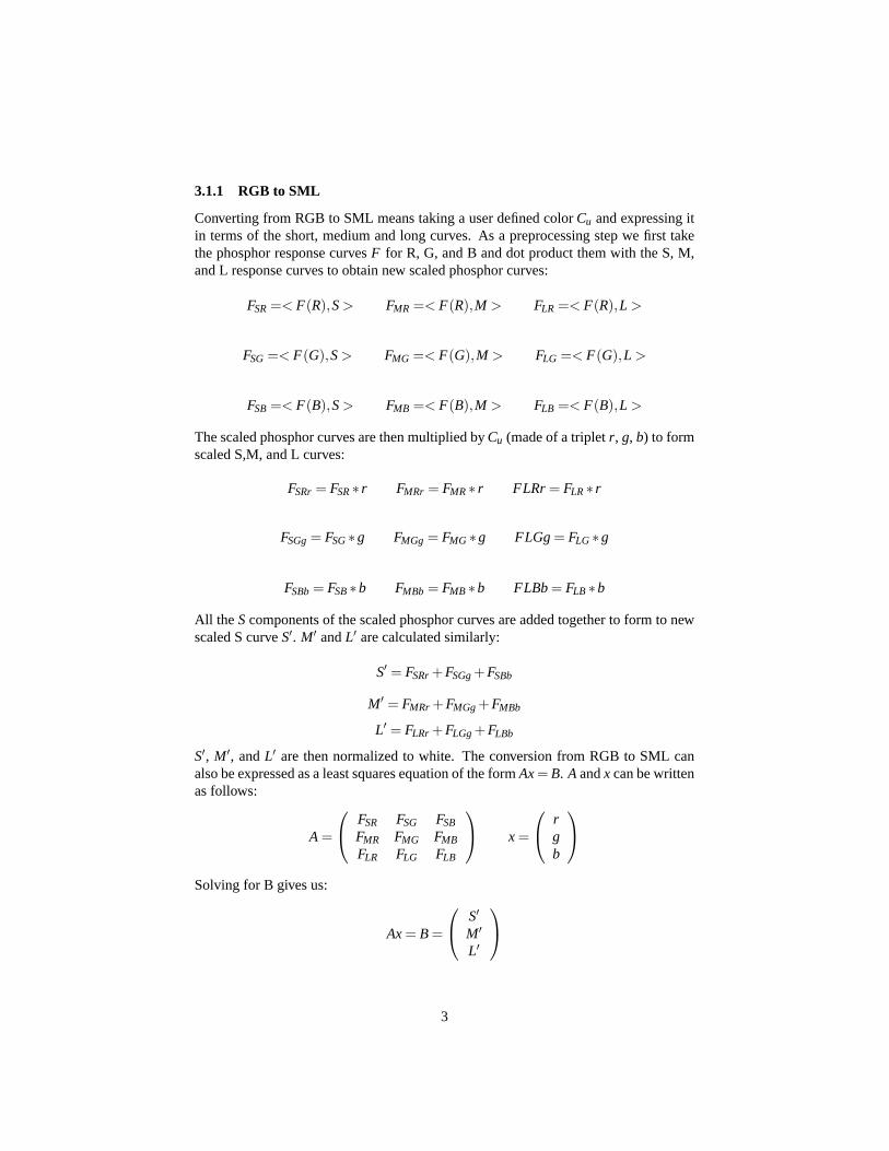
3.1.1 RGB to SML

Converting from RGB to SML means taking a user defined colorCu and expressing itin terms of the short, medium and long curves. As a preprocessing step we first takethe phosphor response curvesF for R, G, and B and dot product them with the S, M,and L response curves to obtain new scaled phosphor curves:

FSR=< F(R),S> FMR =< F(R),M > FLR =< F(R),L >

FSG=< F(G),S> FMG =< F(G),M > FLG =< F(G),L >

FSB=< F(B),S> FMB =< F(B),M > FLB =< F(B),L >

The scaled phosphor curves are then multiplied byCu (made of a tripletr, g, b) to formscaled S,M, and L curves:

FSRr= FSR∗ r FMRr = FMR∗ r FLRr = FLR∗ r

FSGg= FSG∗g FMGg = FMG∗g FLGg= FLG∗g

FSBb= FSB∗b FMBb = FMB∗b FLBb= FLB∗b

All the Scomponents of the scaled phosphor curves are added together to form to newscaled S curveS′. M′ andL′ are calculated similarly:

S′ = FSRr+FSGg+FSBb

M′ = FMRr +FMGg+FMBb

L′ = FLRr +FLGg+FLBb

S′, M′, andL′ are then normalized to white. The conversion from RGB to SML canalso be expressed as a least squares equation of the formAx= B. A andx can be writtenas follows:

A =

FSR FSG FSB

FMR FMG FMB

FLR FLG FLB

x =

rgb

Solving for B gives us:

Ax= B =

S′

M′

L′

3

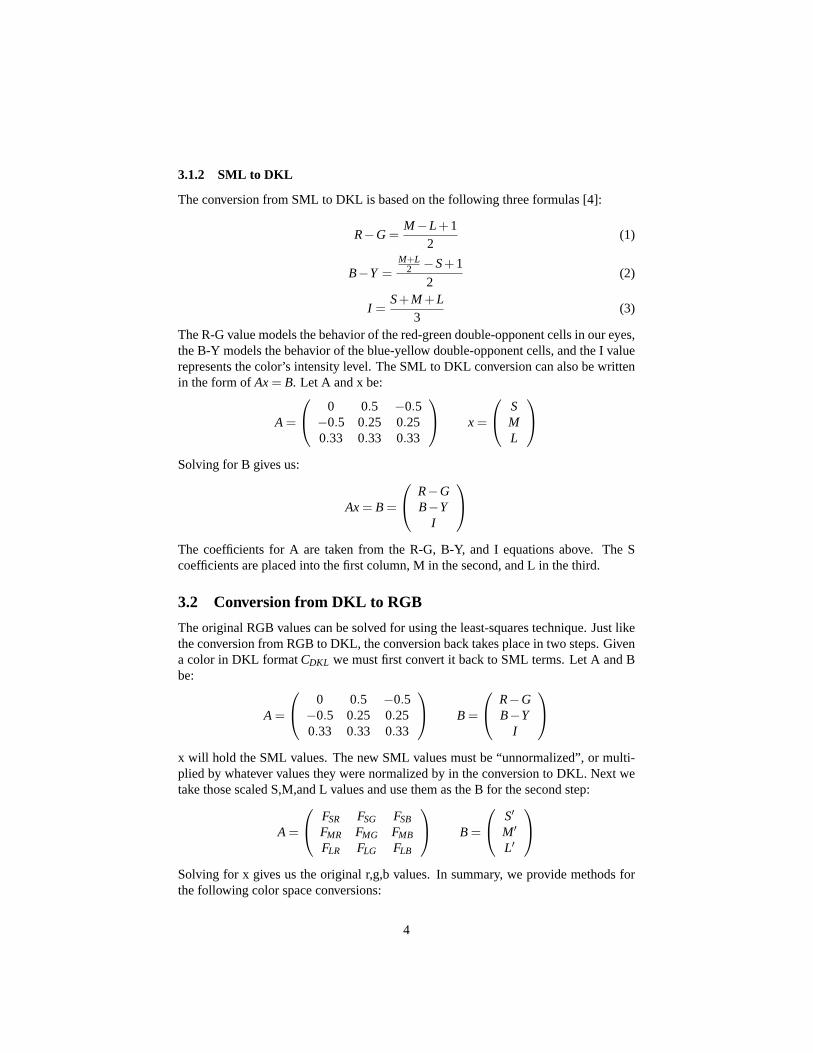
3.1.2 SML to DKL

The conversion from SML to DKL is based on the following three formulas [4]:

R−G =M−L+1

2(1)

B−Y =M+L

2 −S+1

2(2)

I =S+M +L

3(3)

The R-G value models the behavior of the red-green double-opponent cells in our eyes,the B-Y models the behavior of the blue-yellow double-opponent cells, and the I valuerepresents the color’s intensity level. The SML to DKL conversion can also be writtenin the form ofAx= B. Let A and x be:

A =

0 0.5 −0.5−0.5 0.25 0.250.33 0.33 0.33

x =

SML

Solving for B gives us:

Ax= B =

R−GB−Y

I

The coefficients for A are taken from the R-G, B-Y, and I equations above. The Scoefficients are placed into the first column, M in the second, and L in the third.

3.2 Conversion from DKL to RGB

The original RGB values can be solved for using the least-squares technique. Just likethe conversion from RGB to DKL, the conversion back takes place in two steps. Givena color in DKL formatCDKL we must first convert it back to SML terms. Let A and Bbe:

A =

0 0.5 −0.5−0.5 0.25 0.250.33 0.33 0.33

B =

R−GB−Y

I

x will hold the SML values. The new SML values must be “unnormalized”, or multi-plied by whatever values they were normalized by in the conversion to DKL. Next wetake those scaled S,M,and L values and use them as the B for the second step:

A =

FSR FSG FSB

FMR FMG FMB

FLR FLG FLB

B =

S′

M′

L′

Solving for x gives us the original r,g,b values. In summary, we provide methods forthe following color space conversions:

4

• RGB to DKL

• DKL to RGB

• RGB to SML

• SML to RGB

• SML to DKL

• DKL to SML

4 Color Shift Comparison Tables

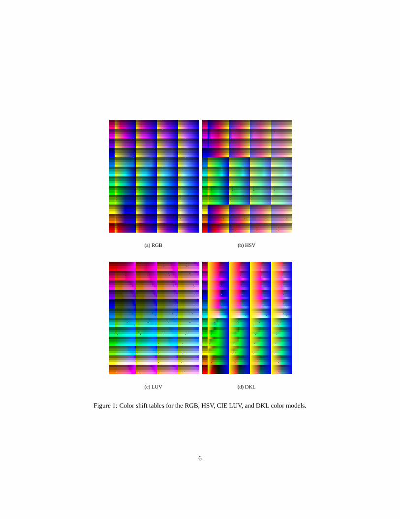
We have developed a technique to generate tables of color shifts that show how a givenhue looks when it is made to be “more warm” or “more cool”. Tables also visuallyshow us the limits of how much a given hue can be shifted before it looses it originalcolor. Some colors can be shifted towards a given warm or cool color more than others.For example, green can be shifted further towards blue than red could. Using a table ofshifts makes this information clear. We have generated color shift tables for the RGB,HSV, CIE LUV, and DKL color spaces, thereby facilitating the comparison of differentcolorspaces’ shifting capabilities. These tables are shown in Figure 1.

We created these tables by first selecting 12 initial hues from around the colorwheel shown in Figure 2(a). These colors have maximum value and saturation. Thehues were placed into a vertical array. Next, we decremented each hue’s value 3 timesand added the resulting hues to the array. They were entered such that the original huewas followed by its 3 value variations. Finally, for each hue in our array (including thevalue variations), we decremented saturation level 3 times. We entered the saturationvariations as a second dimension in our array. For each of the 48 positions in our ver-tical array, we entered 3 additional horizontal entries, corresponding to the saturationvariations (Figure 2(b)). Let these initial hues be referred to as target huesTh. Each huein the 2-d array is then shifted towards a warm and a cool color. Let the warm colorbe denoted asCw and the cool color be denoted asCc. For the tables shown in Figure1, we setCw to yellow andCc to blue. A gradient is generated for each that showsthe shift fromCc, through ourTh, toCw. While the rest of the implementation processdiffers from colorspace to colorspace, the process described here outlines the generalidea used.

4.1 Gradient Generation

Each gradient in the table goes fromCw to Cc, passes throughTh, and a neutralizedversion of thatTh. The initial Th’s are often not neutral colors, but lean more towardsCw or Cc. A neutral version of the particularTh is found and serves as that gradient’smid-point on the shift fromCw toCc. It is equal partsCw andCc. Let the neutralizedTh

be denoted asTn. How the neutral is found depends on the colorspace and onCw andCc. For our purposes, we wanted a neutralized version of theTh that was equal partsyellow and blue.

5

(a) RGB (b) HSV

(c) LUV (d) DKL

Figure 1: Color shift tables for the RGB, HSV, CIE LUV, and DKL color models.

6

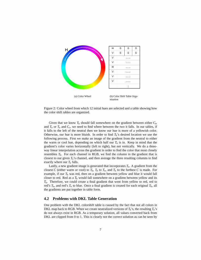
(a) Color Wheel (b) Color Shift Table Orga-nization

Figure 2: Color wheel from which 12 initial hues are selected and a table showing howthe color shift tables are organized.

Given that we knowTh should fall somewhere on the gradient between eitherCw

andTn or Tn andCc, we need to find where between the two it falls. In our tables, ifit falls to the left of the neutral then we know our hue is more of a yellowish color.Otherwise, our hue is more bluish. In order to findTh’s desired location we use thefollowing process. First we make an image of the gradient from the neutral to eitherthe warm or cool hue, depending on which half ourTn is in. Keep in mind that thegradient’s color varies horizontally (left to right), but not vertically. We do a three-way linear interpolation across the gradient in order to find the color that most closelyresemblesTh. For each channel in RGB, we find the column in the gradient that isclosest to our givenTn’s channel, and then average the three resulting columns to findexactly where ourTn falls.

Lastly, a new gradient image is generated that incorporatesTn. A gradient from theclosestC (either warm or cool) toTh, Th to Tn, andTn to the farthestC is made. Forexample, if ourTh was red, then on a gradient between yellow and blue it would fallcloser to red. Red as aTh would fall somewhere on a gradient between yellow and itsTn. Therefore, we could create a final gradient that went from yellow to red, red tored’sTn, and red’sTn to blue. Once a final gradient is created for each originalTh, allthe gradients are put together in table form.

4.2 Problems with DKL Table Generation

One problem with the DKL colorshift table is caused by the fact that not all colors inDKL map back to RGB. When we create neutralized versions ofTh’s, the resultingTn’sdo not always exist in RGB. As a temporary solution, all values converted back fromDKL are clipped from 0 to 1. This is clearly not the correct solution as can be seen by

7

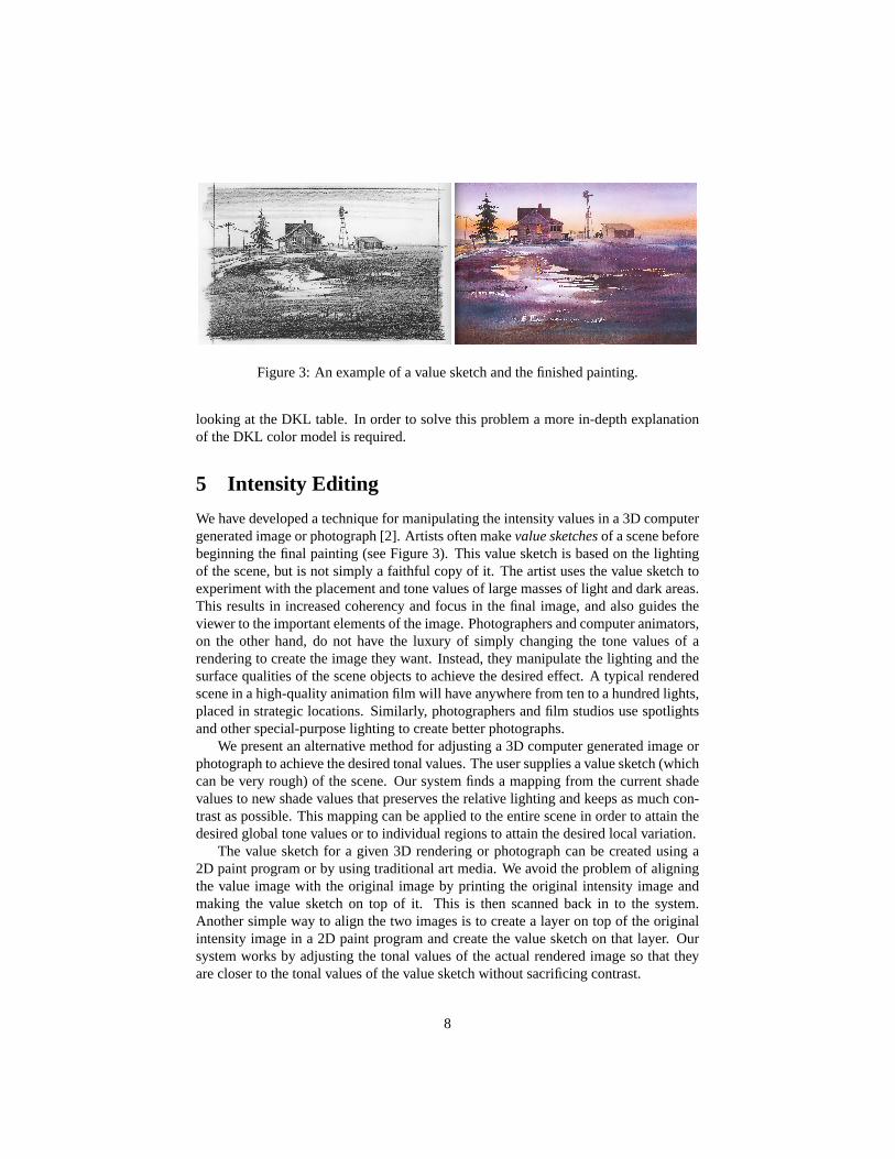
Figure 3: An example of a value sketch and the finished painting.

looking at the DKL table. In order to solve this problem a more in-depth explanationof the DKL color model is required.

5 Intensity Editing

We have developed a technique for manipulating the intensity values in a 3D computergenerated image or photograph [2]. Artists often makevalue sketchesof a scene beforebeginning the final painting (see Figure 3). This value sketch is based on the lightingof the scene, but is not simply a faithful copy of it. The artist uses the value sketch toexperiment with the placement and tone values of large masses of light and dark areas.This results in increased coherency and focus in the final image, and also guides theviewer to the important elements of the image. Photographers and computer animators,on the other hand, do not have the luxury of simply changing the tone values of arendering to create the image they want. Instead, they manipulate the lighting and thesurface qualities of the scene objects to achieve the desired effect. A typical renderedscene in a high-quality animation film will have anywhere from ten to a hundred lights,placed in strategic locations. Similarly, photographers and film studios use spotlightsand other special-purpose lighting to create better photographs.

We present an alternative method for adjusting a 3D computer generated image orphotograph to achieve the desired tonal values. The user supplies a value sketch (whichcan be very rough) of the scene. Our system finds a mapping from the current shadevalues to new shade values that preserves the relative lighting and keeps as much con-trast as possible. This mapping can be applied to the entire scene in order to attain thedesired global tone values or to individual regions to attain the desired local variation.

The value sketch for a given 3D rendering or photograph can be created using a2D paint program or by using traditional art media. We avoid the problem of aligningthe value image with the original image by printing the original intensity image andmaking the value sketch on top of it. This is then scanned back in to the system.Another simple way to align the two images is to create a layer on top of the originalintensity image in a 2D paint program and create the value sketch on that layer. Oursystem works by adjusting the tonal values of the actual rendered image so that theyare closer to the tonal values of the value sketch without sacrificing contrast.

8

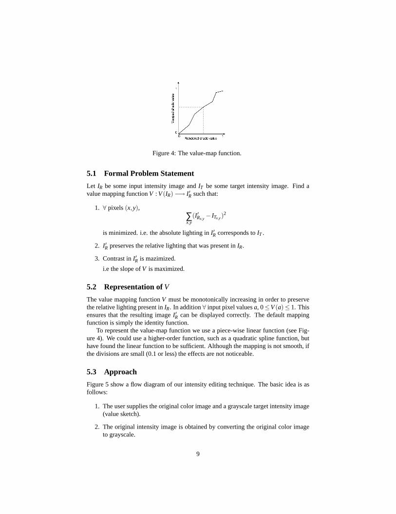
Figure 4: The value-map function.

5.1 Formal Problem Statement

Let IR be some input intensity image andIT be some target intensity image. Find avalue mapping functionV : V(IR)−→ I ′R such that:

1. ∀ pixels(x,y),∑x,y

(I ′Rx,y− ITx,y)

2

is minimized. i.e. the absolute lighting inI ′R corresponds toIT .

2. I ′R preserves the relative lighting that was present inIR.

3. Contrast inI ′R is mazimized.

i.e the slope ofV is maximized.

5.2 Representation ofV

The value mapping functionV must be monotonically increasing in order to preservethe relative lighting present inIR. In addition∀ input pixel valuesa, 0≤V(a)≤ 1. Thisensures that the resulting imageI ′R can be displayed correctly. The default mappingfunction is simply the identity function.

To represent the value-map function we use a piece-wise linear function (see Fig-ure 4). We could use a higher-order function, such as a quadratic spline function, buthave found the linear function to be sufficient. Although the mapping is not smooth, ifthe divisions are small (0.1 or less) the effects are not noticeable.

5.3 Approach

Figure 5 show a flow diagram of our intensity editing technique. The basic idea is asfollows:

1. The user supplies the original color image and a grayscale target intensity image(value sketch).

2. The original intensity image is obtained by converting the original color imageto grayscale.

9

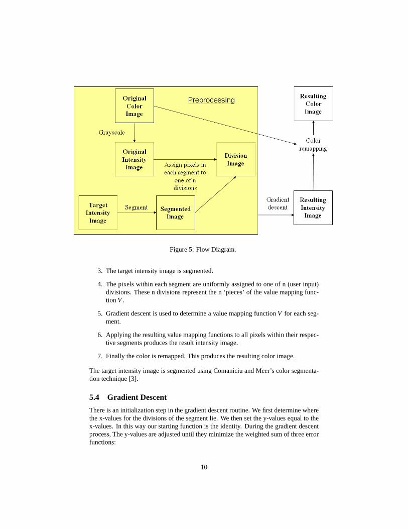
Figure 5: Flow Diagram.

3. The target intensity image is segmented.

4. The pixels within each segment are uniformly assigned to one of n (user input)divisions. These n divisions represent the n ‘pieces’ of the value mapping func-tion V.

5. Gradient descent is used to determine a value mapping functionV for each seg-ment.

6. Applying the resulting value mapping functions to all pixels within their respec-tive segments produces the result intensity image.

7. Finally the color is remapped. This produces the resulting color image.

The target intensity image is segmented using Comaniciu and Meer’s color segmenta-tion technique [3].

5.4 Gradient Descent

There is an initialization step in the gradient descent routine. We first determine wherethe x-values for the divisions of the segment lie. We then set the y-values equal to thex-values. In this way our starting function is the identity. During the gradient descentprocess, The y-values are adjusted until they minimize the weighted sum of three errorfunctions:

10

ErrTot = (WeightA∗ErrA)+(WeightC ∗ErrC)+(WeightM ∗ErrM)

Where:

• ErrTot is the total error

• ErrA is the absolute error

• ErrC is the contrast error

• ErrM is the monotonically increasing error.

• WeightA is the weight for absolute error.

• WeightC is the weight for contrast error.

• WeightM is the weight for monotonically increasing test error.These weights should always sum to 1.0. A detailed explanation of the errorfunctions is presented below.

The absolute error is calculated as follows:

ErrA =∑x,y

∣∣∣(I ′Rx,y− ITx,y)

∣∣∣num pixels

Where

• I ′R is the image generated from some value mapping function.

• IT is the target intensity image.

• (x,y) are all pixels in the segment being processed.

The contrast error is calculated as follows:

ErrC = ∑i |(CurrYvalue[i]−MaxContrastYvalue[i])|numYvals

Where

• CurrYvalue[i] is the current y-value.

• MaxContrastYvalue[i] is the y-value that will maximize contrast.

The monotonically increasing error is calculated as follows:ErrM = 0.0 if CurrYvalue[i +1]−CurrYvalue[i] > 0 ErrM = 1.0 otherwise.

11

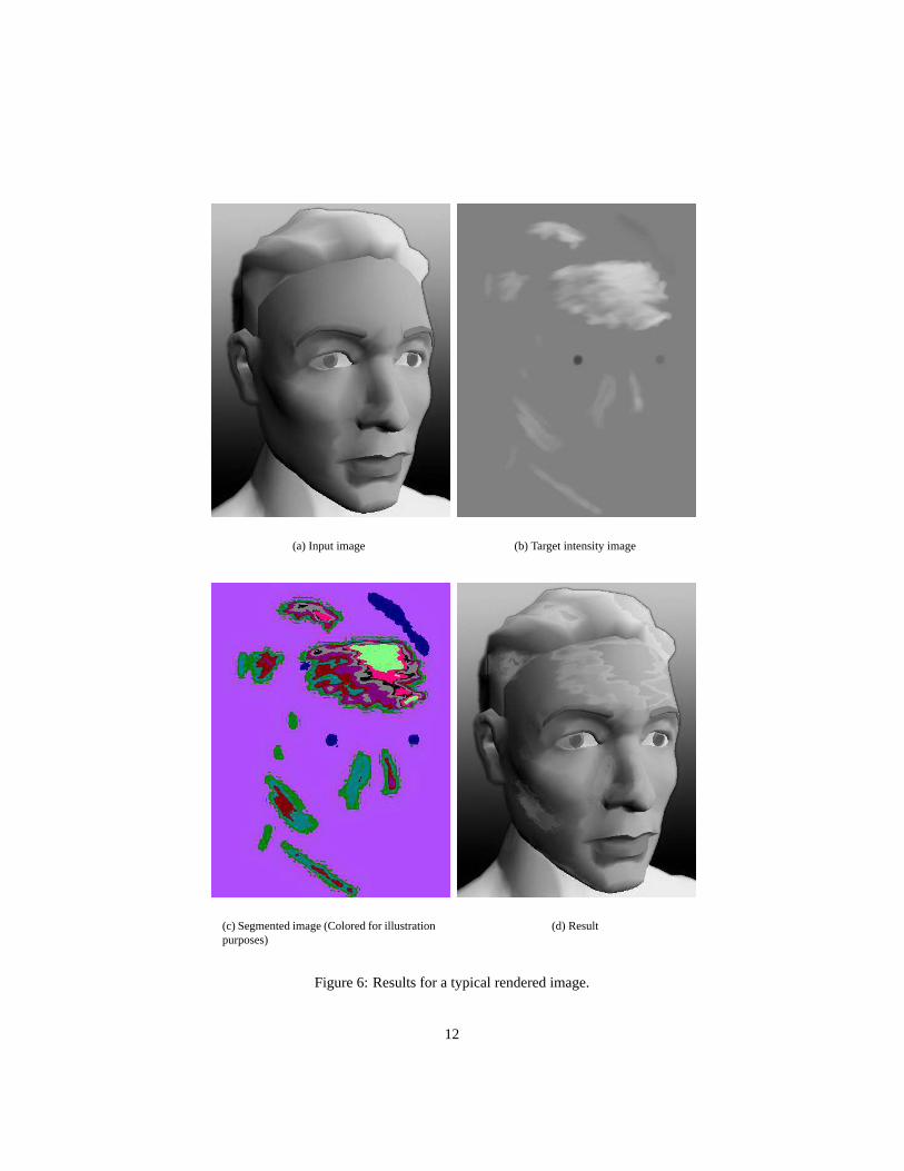
(a) Input image (b) Target intensity image

(c) Segmented image (Colored for illustrationpurposes)

(d) Result

Figure 6: Results for a typical rendered image.

12

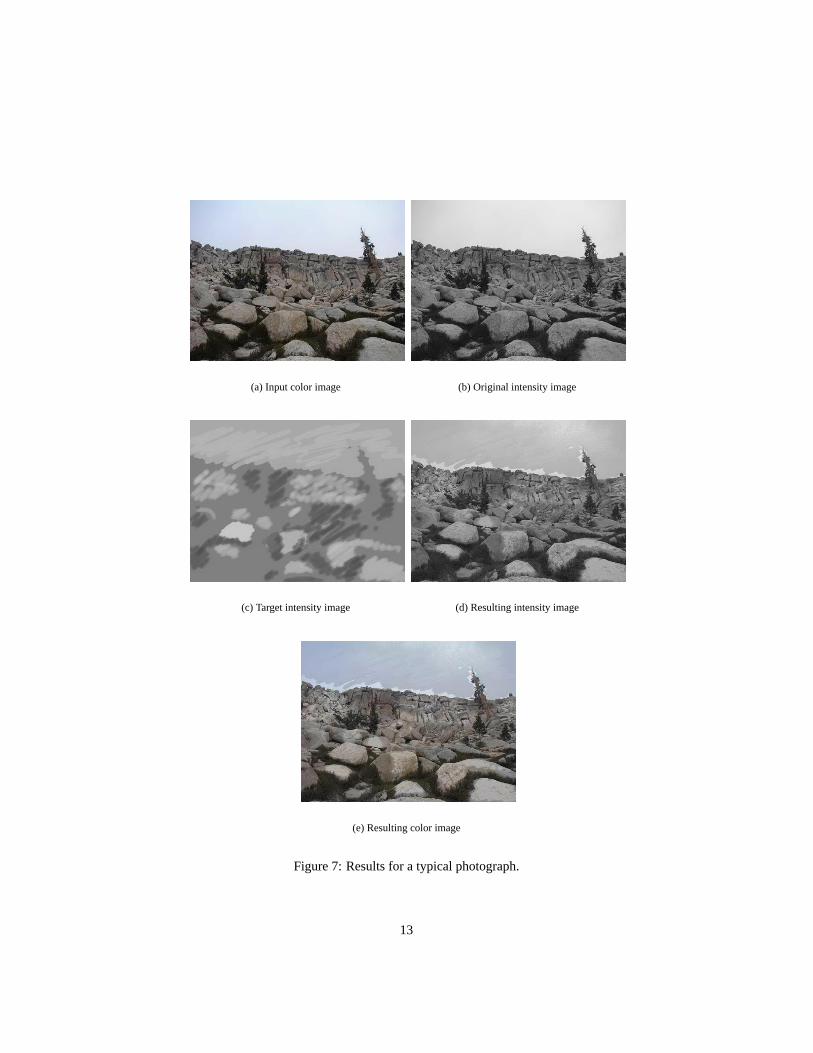
(a) Input color image (b) Original intensity image

(c) Target intensity image (d) Resulting intensity image

(e) Resulting color image

Figure 7: Results for a typical photograph.

13

5.5 Results

Figure 6 and Figure 7 show some results obtained using our intensity editing technique.For the examples, the same weights were used for each segment. This causes the resultsfor some segments to be closer to the target values than others. Evidence of this can beseen in Figure 6 on the forehead where the lightest target area is not the lightest areain the result. We are currently trying to develop techniques that analyze the image andautomatically generate weights for each segment.

6 Current and Future Work

We are currently trying to incorporate the DKL color model with our intensity editingtechnique. We are also working on gaining a better understanding of the DKL colorspace boundary. We plan to incorporate the rod response into our system and developperception based contrast and detail editing techniques.

References

[1] P. Lennie A. M. Derrington, J. Krauskopf. Chromatic mechanisms in lateral genic-ulate nucleus of macaque.Journal of Physiology, 357:241 –265, 1984.

[2] R. Bailey and C. Grimm. Using value images to adjust intensity in 3d render-ings and photographs. 31st International Conference on Computer Graphics andInteractive Techniques, 2004. Presented at Poster Session.

[3] D. Comaniciu and P. Meer. Robust analysis of feature spaces: color image seg-mentation. InProceedings of the 1997 Conference on Computer Vision and PatternRecognition (CVPR ’97), page 750. IEEE Computer Society, 1997.

[4] Krauskopf J. Lennie, P. and G. Sclar. Chromatic mechanisms in striate cortex ofmacaque.Journal of Neuroscience, 10:649 – 669, 1990.

14