Toward Wave-based Sound Synthesis for Computer Animation

JUI-HSIEN WANG, Stanford University

ANTE QU, Stanford University

TIMOTHY R. LANGLOIS, Adobe ResearchDOUG L. JAMES, Stanford University

We explore an integrated approach to sound generation that supports a wide

variety of physics-based simulation models and computer-animated phe-

nomena. Targeting high-quality oline sound synthesis, we seek to resolve

animation-driven sound radiation with near-ield scattering and difrac-

tion efects. The core of our approach is a sharp-interface inite-diference

time-domain (FDTD) wavesolver, with a series of supporting algorithms

to handle rapidly deforming and vibrating embedded interfaces arising in

physics-based animation sound. Once the solver rasterizes these interfaces,

it must evaluate acceleration boundary conditions (BCs) that involve model-

and phenomena-speciic computations. We introduce acoustic shaders as a

mechanism to abstract away these complexities, and describe a variety of

implementations for computer animation: near-rigid objects with ringing

and acceleration noise, deformable (inite element) models such as thin shells,

bubble-based water, and virtual characters. Since time-domain wave synthe-

sis is expensive, we only simulate pressure waves in a small region about each

sound source, then estimate a far-ield pressure signal. To further improve

scalability beyond multi-threading, we propose a fully time-parallel sound

synthesis method that is demonstrated on commodity cloud computing re-

sources. In addition to presenting results for multiple animation phenomena

(water, rigid, shells, kinematic deformers, etc.) we also propose 3D automatic

dialogue replacement (3DADR) for virtual characters so that pre-recorded

dialogue can include character movement, and near-ield shadowing and

scattering sound efects.

CCS Concepts: · Computing methodologies → Physical simulation;

Additional Key Words and Phrases: Computer animation, sound synthesis,

inite-diference time-domain method, acoustics

ACM Reference Format:

Jui-Hsien Wang, Ante Qu, Timothy R. Langlois, and Doug L. James. 2018.

Toward Wave-based Sound Synthesis for Computer Animation. ACM Trans.

Graph. 37, 4, Article 109 (August 2018), 16 pages. https://doi.org/10.1145/

3197517.3201318

1 INTRODUCTION

Recent advances in physics-based sound synthesis have led to im-

proved sound-generation techniques for computer-animated phe-

nomena, including water, rigid bodies, deformable models like rods

Authors’ addresses: Jui-Hsien Wang, Stanford University, jui-hsien.wang@stanford.edu; Ante Qu, Stanford University, antequ@cs.stanford.edu; Timothy R. Langlois, AdobeResearch, tlangloi@adobe.com; Doug L. James, Stanford University.

Permission to make digital or hard copies of all or part of this work for personal orclassroom use is granted without fee provided that copies are not made or distributedfor proit or commercial advantage and that copies bear this notice and the full citationon the irst page. Copyrights for components of this work owned by others than ACMmust be honored. Abstracting with credit is permitted. To copy otherwise, or republish,to post on servers or to redistribute to lists, requires prior speciic permission and/or afee. Request permissions from permissions@acm.org.

© 2018 Association for Computing Machinery.0730-0301/2018/8-ART109 $15.00https://doi.org/10.1145/3197517.3201318

and shells, ire, and brittle fracture. However, unlike visual render-

ing techniques which are slow but capable of generating very high-

quality, general-purpose results during parallel oline rendering,

current methods for sound synthesis sufer from several fundamen-

tal deiciencies that limit high-quality renderings. First, because

of the high space-time complexity of sound modeling and compli-

cated acoustic phenomena, many modeling approximations (lin-

earizations, simpliied radiation, etc.) and algorithmic optimizations

(precomputation, data-driven methods, etc.) are typically made for

tractability and to improve performance, but can limit sound quality

and the range of physical phenomena that can be considered. Sec-

ond, the proliferation of real-time, object-level and/or phenomena-

speciic sound models has led to a lack of integrated wave modeling,

wherein it is diicult to combine models and have them support

inter-model acoustic interactions, such as shadowing and scattering.

The end result is that there is no practical general-purpose solu-

tion (regardless of performance) for practitioners to author general

animations with integrated sound synthesis. In contrast, we seek

a general rendering approach where, given an animation, say of a

crash cymbal being hit (see Figure 1), one can just łhit the render

button and wait,ž to get the high-quality result.

Fig. 1. Crash! Soundwaves radiate of a visibly deforming crash cym-

bal: Our sharp-interface finite-diference time-domain (FDTD) wave solver

can synthesize sound sources with rapidly deforming interfaces, such as

this thin-shell model, or even water, using a single integrated approach.

In this paper, we explore oline wave-based sound synthesis tech-

niques that can generate high-quality animation-sound content for

general-purpose dynamic scenes and multi-physics sound sources.

The general-purpose integrated approach is inherently extremely

slow, but enables łwhat ifž exploration of the rich range of sounds

possible from complex animated phenomena (such as splashing

water), and to better understand future challenges and needs for

animation sound. We humbly liken our approach to early łwhat ifž

digital image synthesis eforts three decades ago, such as the łone

frame moviež generated in the ‘80s by the aspiring REYES (łRenders

Everything You Ever Sawž) 3D rendering system [Cook et al. 1987]

that łdemonstrated, at least theoretically, the possibility of creating

109:2 • J.-H. Wang et al.

Frequency-domain radiation [Langlois et al. 2016]

Time-domain radiation [Our Method]

Fig. 2. Dramatically Improved Water Sounds: (Botom, let) Using

water simulation and surface vibration data from [Langlois et al. 2016],

we simulated (Botom, right) acoustic waves emited from the rapidly

deforming and vibrating fluid-air interface using our FDTD solver (in

this 2D slice, the rigid container is colored black, and the water is solid

blue). Interactions with the container and water surface geometry cause

complex time-varying radiation paterns, cavity resonances, and dramati-

cally enhance the sound compared to the prior frequency-domain bubble

radiation model. Spectrograms clearly demonstrate (Top) missing high-

frequency detail in the prior approach whereas (Middle) our approach

produces renderings with enhanced high-frequency content, that tend to

produce more natural water sounds that are less harsh.

full length sequences, or even a feature ilm, composed of images

which matched the quality of 35mm ilmž [Cook 2015], as opposed

to a tweak on existing rendering methods [Heckbert 1987]. The

theme of this paper is to irst know what we want to compute and

how, and then, later, we will optimize, design, and build parallel

systems to do it fast. Our initial explorations have already shown a

vastly richer class of sounds are possible, such as for bubble-based

water animations (see Figure 2).

To resolve complex sound radiation, near-ield scattering and

difraction efects, we rely on a general-purpose pressure-based

inite-diference time-domain (FDTD) wavesolver. We describe a

series of methods to support embedded geometric interfaces and to

impose Neumann (acceleration) boundary conditions (BCs) on them

using a ghost-cell technique. Once the solver rasterizes these inter-

faces, it then evaluates the acceleration BCs prescribed by model-

and phenomena-speciic computations (assuming a one-way cou-

pling łanimation to soundž approach). We introduce acoustic shaders

as a computational abstraction of the various simulation-level details

needed to evaluate (usually Neumann acceleration) BCs at audio-

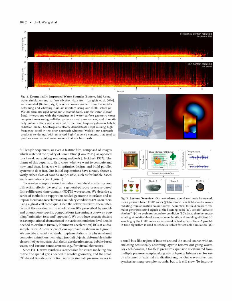
sample rates. An overview of our approach is shown in Figure 3.

We describe a variety of shader implementations for physics-based

computer animation: near-rigid (modal) objects, deformable (inite

element) objects such as thin shells, acceleration noise, bubble-based

water, and various sound sources, e.g., for virtual characters.

Since FDTD wave synthesis is expensive for source modeling due

to the ine spatial grids needed to resolve geometry, and the small

CFL-based timestep restriction, we only simulate pressure waves in

Output Sound

Point 0:

Point N:

Input Animation

Schedule

r

Acoustic Shader Interface

Far-

field

Estim

ate

Sharp-Interface FDTD Solver

Shader 1 Shader 2 Shader 3 Shader S

Fig. 3. System Overview: Our wave-based sound synthesis framework

uses a pressure-based FDTD solver (ğ3) to resolve near-field acoustic waves

radiating from animation-sound sources. A practical far-field pressure esti-

mator generates sound signals at the listening point (ğ5). We use łacoustic

shadersž (ğ4) to evaluate boundary condition (BC) data, thereby encap-

sulating simulation-level sound-source details, and enabling eficient BC

sampling by the FDTD solver on rasterized embedded interfaces. A parallel-

in-time algorithm is used to schedule solves for scalable simulation (ğ6).

a small box-like region of interest around the sound source, with an

enclosing acoustically absorbing layer to remove out-going waves.

For each domain, a far-ield pressure expansion is estimated from

multiple pressure samples along any out-going listener ray, for use

by a listener or external auralization engine. Our wave-solver can

synthesize many complex sounds, but it is still slow. To improve

Toward Wave-based Sound Synthesis for Computer Animation • 109:3

performance beyond thread-level parallelism, we demonstrate a

time-parallel method for sound-source evaluation that exploits the

linear dependence of the sound on the nonzero boundary data. Fi-

nally, we demonstrate various results for rigid bodies, nonlinear thin

shells, water, etc., evaluated using commodity cloud computing re-

sources. In addition, we demonstrate 3D automatic dialogue replace-

ment (3DADR) for virtual characters that processes pre-recorded

dialogue to include character movement, and near-ield shadowing

and scattering sound efects.

2 RELATED WORK

Sound rendering has a long history in computer graphics and an-

imation [Takala and Hahn 1992] and interactive virtual environ-

ments [Begault 1994]. While most sound efects can be achieved

using recordings, data-driven methods, procedural audio efects,

and other creative means, there is a long history in computer sound

and music of physics-based methods used for non-visual/audio-only

sound generation [Cook 2002; Gaver 1993; Smith 1992]. The process

by which a sound ield in a virtual space is rendered audible to

a binaural listener at a speciic position in space is referred to as

auralization [Kleiner et al. 1993; Vorländer 2008], and for practical

reasons it is usually broken into three stages: (1) sound genera-

tion/synthesis, (2) sound propagation throughout the scene, and

(3) binaural listening. Our approach concerns the irst stage (sound

generation for oline computer animation), but also touches on

near-ield sound propagation and related numerical wave simula-

tion techniques. In oline computer animation, most sound tracks

are composed using digital audio workstations (DAWs), such as Pro

Tools [Avid Technology 2018], which can record and mix audio,

and apply various efects (such as reverb) during audio post pro-

duction. Our approach is complementary to existing methods, in

that it enables another way to generate (3D) sound clips that are

synchronized with animated content.

Prior works on animation-sound have modeled sound radiation

from animated solids and luids in a wide variety of ways, ranging

from completely ignoring it, to approximating in any number of

ways for convenience and speed. Rigid-body sound models based

on decoupled linear modal oscillators have been widely considered

since the ‘90s [Cook 2002; van den Doel and Pai 1998], and have

long enjoyed real-time performance and acceleration [Bonneel et al.

2008]. Detailed wave radiation is usually ignored, with the amplitude

of the oscillators displayed directly, possible with calibration from

recordings [van den Doel et al. 2001] or material parameters hand

tuned for plausibility [O’Brien et al. 2002].

Precomputed acoustic transfer [James et al. 2006] was introduced

to provide real-time estimation of acoustic pressure amplitudes for

harmonicmodal vibrations, and leveraged precomputed radiation so-

lutions to the Helmholtz equation. While the method could account

for realistic sound amplitudes from linear modal vibration mod-

els, it had several shortcomings including assumptions of linearized

small-amplitude modal dynamics, pure harmonic oscillations (which

poorly approximate the transients following contact events), and

the inability of nearby objects to inluence each other acoustically,

e.g., shadowing and interrelections. All of these assumptions are

no longer necessary using our general FDTD synthesis framework.

Precomputed acceleration noise [Chadwick et al. 2012a,b] was

introduced to account for transient łclickingž sounds due to hard

rigid-body accelerations that dominate ringing (modal) noise for

small objects. The approach also used a FDTD method to estimate

far-ield radiation. However, we do not precompute these object-

speciic separate responses for interactive performance, but instead

compute both ringing (modal) and acceleration noise efects on-the-

ly simultaneously using a single waveield in our general FDTD

synthesis framework.

O’Brien et al. [2001] also proposed a time-domain sound synthesis

framework that could render audio-rate vibrations of nonlinear de-

formable inite-element models, employing a ray-based attenuated

delay-line model of radiation. While slow at the time (primarily due

to high explicit time-stepping costs of nonlinear FEMmodels) a very

wide variety of animations and sounds were possible. We propose

a wave-based FDTD framework that more accurately accounts for

soundwave radiation (and scattering). Although the computational

cost is higher, wave phenomena are critical to predictive modeling

of realistic radiated sounds.

More complex animation-sound phenomena have been consid-

ered that would also beneit from our high-quality FDTD sound

synthesis framework. Eicient reduced-order models of near-rigid

thin shells were considered in [Chadwick et al. 2009], but could not

simulate large deformations (due to mode locking). Furthermore,

the linear acoustic transfer model is technically incorrect since the

modal oscillators are not frequency localized due to nonlinear mode

coupling. Schweickart et al. [2017] synthesized sounds from elastic

rods, and supported large deformations, such as for a Slinky falling

down stairs, and used a precomputed dipole radiation model, but

did not support scattering nearby surfaces or itself. Cloth and paper

sound synthesis have been explored using various highly specialized

techniques which address challenges due to the diiculty of direct

numerical simulation of highly nonlinear deformations, vibrations,

and acoustic emissions [An et al. 2012; Cirio et al. 2016; Schreck et al.

2016]. Chadwick and James [2011] synthesized combustion sounds

using a hybrid simulation and data-driven approach. In contrast,

our approach supports radiation from highly deforming interfaces,

makes no assumptions about the underlying vibration model or

linearity, and can capture full spectrum behavior, possibly removing

the dependence on data-driven techniques.

Zheng and James [2010] synthesized brittle fracture sounds us-

ing rigid-body sound models based on linear modal analysis and

precomputed acoustic transfer. Unfortunately every fracture event

invalided the precomputed models, and led to expensive acous-

tic transfer re-computations. In contrast, by resolving each object’s

sound radiation on a shared FDTDwaveield grid, extensive precom-

putation of object-speciic sound radiation models can be avoided.

The modeling of water sounds goes back to Minnaert’s classical

bubble vibration model [Minnaert 1933], which van den Doel [2005]

used in modal sound banks for real-time audio-domain synthesis

of stochastic water sounds without radiation modeling. Similar

single-frequency bubble models were considered [Moss et al. 2010;

Zheng and James 2009]. The latter method explored a per-bubble

Helmholtz acoustic transfer model to better estimate the sound ra-

diation, resulting in thousands of exterior fast multipole Helmholtz

radiation solves per animation-sound clip. Improved two-phase

109:4 • J.-H. Wang et al.

incompressible luid-air modeling, and capacitance-based bubble

frequency estimation were introduced in [Langlois et al. 2016], and

combined with an acoustic transfer model similar to [Zheng and

James 2009]. In contrast, we use a FDTD solver to better account for

the air-borne sound waves, and the related transient radiation and

scattering details which are perceptually signiicant (see Figure 2).

While FDTD solves are expensive, they can actually be far cheaper

(but less parallel) than the thousands to millions of per-bubble exte-

rior Helmholtz radiation solves, since the radiation of all bubbles

are resolved simultaneously by one FDTD wave simulation.

Methods for sound propagation modeling in interactive virtual

environments have been explored for decades, and are increas-

ingly used to produce interactive reverb efects for point-like sound

sources, e.g., of a sound recording. For large architectural and out-

door environments, geometric propagation techniques (e.g., ray-

based methods) are most popular for approximating occlusion and

scattering efects. Examples include methods based on beam tracing

[Funkhouser et al. 1998, 1999], or frustum tracing [Chandak et al.

2008], extensions to capture difraction around corners using the

uniform theory of difraction [Tsingos et al. 2001], higher-order

difraction efects [Schissler et al. 2014], or hybrid approach based

on spatial/frequency decomposition [Yeh et al. 2013]. Wave-based

sound propagation techniques are less practical for interactive ap-

plications unless precomputations and approximations are used:

notable recent innovations include adaptive rectangular decom-

positions [Raghuvanshi et al. 2009], equivalent source approxima-

tions [Mehra et al. 2013], and parametric wave ield coding [Raghu-

vanshi and Snyder 2014]. For performance reasons, and to admit

preprocessing, methods often make assumptions, such as a static

environment. In contrast, our work applies to oline sound source

modeling in smaller domains where strong difraction and wave

efects preclude the use of geometric/ray-based approaches, and

highly deforming interfaces and animated phenomena preclude the

use of many precomputation techniques.

Finite-diference time-domain (FDTD) methods [Larsson and

Thomée 2009] and digital waveguides [Smith 1992] have long been

used to approximate solutions to the wave equation, and fundamen-

tal stability and accuracy bounds are relatively well understood.

Thanks to computational advances, a number of recent papers have

started to use FDTDmethods to solve wide-bandwidth acoustic radi-

ation problems in applications such as computational room acoustics

[Bilbao 2013], musical instrument design [Bilbao 2009], and head-

related transfer function computation [Meshram et al. 2014]. Due to

advanced parallel hardware such as GPUs and the scalable perfor-

mance of FDTD, there are also a number of recent papers exploring

the use of FDTD methods to achieve high-throughput [Mehra et al.

2012; Micikevicius 2009] or even real-time wave simulation [Allen

and Raghuvanshi 2015], as well as using large GPU clusters to per-

form fast seismic modeling (elastic waves) [Komatitsch et al. 2010]

and electrodynamics simulations [Talove and Hagness 2005]. Partic-

ularly noteworthy is the work at the University of Edinburgh by Ste-

fan Bilbao, Craig Webb and others on GPU-accelerated FDTD sound

simulations of musical instruments, such as a timpani drum [Bilbao

and Webb 2013], a snare drum [Bilbao 2011], and digital musical ar-

rangements (see Webb’s Ph.D. thesis [Webb 2014]), which is similar

in spirit to our general-purpose approach, although we can not rely

on rigid, rasterized geometry in computer animation.

Simulating acoustic waves in a dynamic environment is less ex-

plored. A notable exception is the paper by Allen et al. [2015], which

simulates virtual instruments that can have time-varying geometric

features, such as opening and closing of tone holes. The geometry

transition was made smooth by the use of a time-varying perfectly

matched layer (PML), which blends the momentum equation and

boundary condition enforcement. Although it works well for creat-

ing/removing walls for the instrument, the blending function can

afect the transients of the sound and this formulation seems ill-

suited for handling general rigid-body transformations and object

deformations for animation.

3 ACOUSTIC WAVE SOLVER

We now describe the core FDTD acoustic wave solver used in our

approach, beginning with some background material (ğ3.1). To com-

pute high-quality, low-noise pressure signals, we employ a high-

order boundary samplingmethod for enforcing the Neumann bound-

ary conditions. The method is explained in ğ3.2 and ğ3.3, where we

discuss the accurate acoustic BC enforcement on static interfaces

using a ghost-cell formulation, and the time-consistent interface

tracking method, respectively.

3.1 Background Material on FDTD Acoustics

Acoustic Wave Equation. Consider a simple scene with a single

(dynamic) object, O . Let Ω ⊂ R3 be the open set containing the

surrounding acoustic medium, and Γ be the boundary of this set

restricted to O’s surface. Pressure perturbations in Ω are governed

by the acoustic wave equation

∂2p (x , t )

∂t2= c2∇2p (x , t ) + cα∇2

∂p (x , t )

∂t, x ∈ Ω, (1)

where c is the speed of sound in the medium (343.2 m/s in air at

standard temperature and pressure), and α is a constant coeicient

that controls damping from air viscosity (derived from linearizing

the Navier-Stokes equation [Morse and Ingard 1968; Webb and

Bilbao 2011]). The Neumann boundary condition enables surface

accelerations to generate waves:

∂np (x , t ) (x ) = −ρan (x , t ), x ∈ Γ, (2)

where ρ is themedium density (1.2041 kg/m3 for air),n is the normal

vector at the surface position, ∂np (x , t ) is the normal pressure gra-

dient and an is the normal surface acceleration. Intuitively, nonzero

surface acceleration on O leads to pressure disturbances, which

travel outwards through Ω and are perceived as sound when they

reach our ears. The linear wave equation is valid whenever O’s

boundary velocity is much lower than c , which is true in our appli-

cation domain.

Finite-diference simulation. We solve the wave equation using the

inite-diference time-domain method (FDTD) [Larsson and Thomée

2009] on a regular, collocated pressure grid. We use the standard 2nd-

order centered diference in space and time. Speciically, suppose we

allocate a grid of cell size h and time step size τ , then the pressure

Toward Wave-based Sound Synthesis for Computer Animation • 109:5

update at cell (i, j,k ) can be expressed as

pn+1i, j,k= (2 + (c2τ 2 + cατ )∇2)pn

i, j,k− (1 + cατ ∇2)pn−1

i, j,k, (3)

where pni, j,k

≡ p (ih, jh,kh,nτ ) is the discretized pressure. ∇2 is the

7-point discrete Laplacian deined as

h2∇2pi, j,k = pi−1, j,k + pi+1, j,k + pi, j−1,k + pi, j+1,k (4)

+ pi, j,k−1 + pi, j,k+1 − 6pi, j,k . (5)

The grid cell size, h, is selected based on the scene and the desired

frequency resolution (see ğ7.1.1). Given h, the time step size, τ , is

chosen as the maximum value that satisies the stability bound,

τc ≤√

α2 + h2/3 − α , set by the Courant-Friedrichs-Lewy (CFL)

condition in 3D [Bilbao 2009]. Note that to leading order, the time

step size is proportional to the cell size.

Absorbing Boundary Conditions. When performing FDTD acous-

tic wave simulations in a inite domain, it is typical to implement

either absorbing boundary conditions (ABCs) [Clayton and Engquist

1977] or perfectly matched layers (PMLs) [Chadwick et al. 2012b; Liu

and Tao 1997] at the grid boundary to minimize artiicial relections.

To accommodate moving objects and to maintain consistency with

the pressure collocated grid, we adopt the computationally simpler

Engquist-Majda type ABC [Bilbao 2011; Engquist and Majda 1977].

More speciically, we have found that a split-ield PML [Liu and Tao

1997], which relies on staggered pressure-velocity grids, can cause

interpolation inconsistency if an object passes through the grid

boundary (see ğ3.3). In constrast, the EM-ABC allows us to more

aggressively place small domains around localized sound sources.

For example, for 3D dialogue re-recording, we can place a domain

just around a character’s head, with the torso passing through the

domain boundary without causing problems. Please see Appendix B

for more details on the ABC implementation.

3.2 Accurate Object Interface Tracking

We describe a high-order boundary sampling method for enforcing

the Neumann BC (2) in this section. Compared to a 1st-order stair-

casing boundary approximation, our method tracks the positions

of the embedded interfaces on the subgrid level and respects the

surface normals when discretizing BCs, which results in smoother

scattering ield, less distorted radiation patterns (Figure 4), and re-

solves more high-frequency content (Appendix C). Compared to

other high-order boundary handling methods in acoustics literature,

our method has smaller overhead as there is no need to remesh

the domain [Bilbao 2013; Botteldooren 1994] or determine cut-cell

volumes [Tolan and Schneider 2003]. Other local conforming meth-

ods [Häggblad and Engquist 2012] might not generalize well to

non-zero BCs and dynamic scenes. Our method has the spirit of

the immersed boundary methods in computational luid dynam-

ics [Fedkiw et al. 1999; Mittal et al. 2008; Mittal and Iaccarino 2005;

Peskin 1981], where the efects of the boundaries are computed and

stored directly on the grid. Because no remeshing is required, it is

ideal for dynamic simulations. We modiied the method from [Mittal

et al. 2008] for acoustic simulation on a pressure collocated grid. In

addition, we avoided the ill-conditioned local solves by hybridizing

1st- and 2nd-order boundary handling to maximize solve eiciency.

(a) (b) (c) (d)

Sta

irca

sin

gO

ur

me

tho

d

Active Sound Object Passive Sound Object

Fig. 4. Ourmethod producesmore uniform radiation paterns for ac-

tive sound objects and eliminates spurious high-frequency artifacts

and noise in the scatering response for passive sound objects: Our

method (Botom row) outperforms the popular staircasing approximation

(Top row) for embedding objects onto the simulation grid. Red represents

positive pressure, blue represents negative pressure, and white represents

the embedded object. (a) spherical monopole sound source radiating well

below the grid resolution limit at 3.4 kHz; (b) spherical monopole sound

source radiating at the grid resolution at 8.7 kHz (our method produces

a more uniform sound field); (c) passive plate scaterer; (d) passive sphere

scaterer.

Rasterization Cell Classification Compute Sample Pts

Fluid Cell

Ghost Cell

Solid Cell

Fig. 5. Building the simulation grid topology. Our method starts by

rasterizing the interfaces to the simulation grid and identifying a set of solid

cells. Among these solid cells, those that have at least one neighbouring

fluid cell are classified as ghost cells, which will be used to compute and

store boundary condition data.

At every step, the interface is irst rasterized to the grid and a

set of ghost cells, xд , are located to store the BCs (see Figure 5).

The observation is that if we assign pressure values to these cells,

pд , then we can carry out FDTD timestepping (3) normally as if

there are no objects or interfaces. The boundary efects are therefore

immersed in the grid. For each ghost cell xд , we irst ind a boundary

point xb ∈ Γ closest to xд , and then approximate the Neumann

boundary condition (2) using 2nd-order centered diferencing

pr − pд

l= −ρan (xb , t ) + O (l

2), (6)

where pr = p (xr , t ), pд = p (xд , t ), l = |xr − xд |, and xr is the

relection point, deined by xr = xд + 2(xb − xд ). See Figure 6 for

an illustration. We sample an from the corresponding sound source

using acoustic shaders, which will be explained in ğ4. The pressure

at the relection point, pr , is estimated using trilinear interpolation

over the surrounding 8 cells. For the derivation below, we use Ωr

to denote this cubic region where the interpolant is valid.

109:6 • J.-H. Wang et al.

Solid cell

Ghost cell

Bulk cell

Active ghost cell

Reected ghost cell

Interpolant region

2ND-ORDER APPROX.

1ST-ORDER APPROX.

Fig. 6. Ghost cell reflection: To find the reflection of a ghost cell located

at xд , we first find a surface boundary point xb closest to xд , then construct

a reflection stencil to impose the Neumann boundary condition. xb can be

found eficiently using spatial acceleration data structures (we used KD-tree

for rigid interfaces and spatial hashing for deformable interfaces).

Since trilinear interpolation can involve other unknown ghost

cells, estimating ghost-cell pressures will, in general, require solving

a sparse linear system. We now describe how to construct this

system. Let

p (x ) = ϕ (x ) · c, x ∈ Ωr , (7)

represent trilinear interpolation, with some unknown coeicients

c ∈ R8, and the polynomial basis row vector ϕ : R3 → R8,

ϕ (x ) = [xyz xy yz xz x y z 1]. (8)

Requiring the interpolant to reconstruct eight adjacent pressure

samples, p ∈ R8, at the sampled cell positions, xi 8i=1, yields the

linear system

Φc =

ϕ1

ϕ2...

ϕ8

c = p. (9)

where ϕi ≡ ϕ (xi ). When one of the interpolation stencils involves

the unknown itself at xд , degeneracy in (6) can happen as l → 0 and

the problem becomes singular. To avoid the singularity, we replace

a row of Φ using the Neumann BC when this happens, similar to

[Mittal et al. 2008]. Concretely, since xb is guaranteed to be in

Ωr , the normal derivative of the interpolant (7) must follow the

Neumann BC at xb :

∂np (xb ) = ∂nϕ (xb ) · c = −ρ an (xb ). (10)

Since the only unknown in this equation is c , we can use this rela-

tionship to replace a row of the linear system in (9) without changing

the interpolant. Let the jth row be the one contributed by xд , then

we replace the jth row of (9) with (10) and obtain Φc = p. We use

SVD decomposition to solve the system

c = Φ−1p. (11)

We can then evaluate the interpolant at xr to get pr = ϕ (xr ) ·

Φ−1p. Substituting this back to (6), we derive a scalar equation for

computing the ghost cell pressure pд .

pд − ϕ (xr ) · Φ−1p = lρ an (xb , t ). (12)

Note that in general p involves pressure values of other ghost cells,

which are unknowns coupled to pд . Applying (12) to Nд ghost

pressure samples gives us a sparse linear system, Aд = b, where A

is of size Nд-by-Nд and д is the vector of all ghost cell pressures. A

is a sparse matrix (number of non-zero entries is upper bounded

by 8Nд ). We solve the linear system using BiCGStab, and observe

stable and fast convergence for all of our examples. Since A only

depends on the position of the interfaces, it can be precomputed

and cached for static scenes.

In Appendix A, we show that the interpolation matrix Φ can be

ill-conditioned. When this occurs, the weights for the trilinear in-

terpolation can grow unbounded and cause pressure instabilities. In

our hybrid approach, we compute the condition number of Φ from

the SVD decomposition, and aborted the high-order solve when it

exceeds a user-deined threshold, κ. In this case, we directly set the

relected point to the corresponding grid-aligned neighbouring cell,

xr ← xn . Equation 12 is then collapsed to the 1st-order staircasing

estimator, pд − pn = lρ an (xb , t ). Note that κ = ∞ yields 2nd-order

accuracy and κ = 0 yields 1st-order accuracy. We observed κ ≈ 25

is suicient to maintain a low replacement rate without instabil-

ity; since trilinear interpolation is translation and scale-invariant,

stencils in (12) are transformed to the [−1, 1]3 cube before evalua-

tion, thus permitting a constant threshold value κ for all examples.

Please see Appendix C for more analysis on the accuracy of interface

tracking.

3.3 Time-consistent Dynamic Interface Tracking

We now describe a method to track the pressure ield with dynami-

cally embedded interfaces, allowing plausible sounds to be produced

by animations, such as the familiar spolling bowl (see Figure 7). Inter-

face movements create discrete cell łjumpsž that can cause audible

pops in the generated sound if care is not taken. More speciically,

when a cell transitions from a łsolidž to łluidž cell, a robust ex-

trapolation procedure is needed to estimate the pressure history

of the cell, otherwise the time-curvature estimation of the wave

equation (1) will fail, and this will lead to a pressure discontinuity,

and possible łpopž sound artifacts and noise. In the CFD literature,

this is known as the fresh-cell problem [Mittal and Iaccarino 2005].

Instead of a more expensive global solve, such as in [Mittal et al.

2008], we compute the fresh-cell pressures locally. For a freshly ap-

pearing cell located at xf , we ind a closest point xb on the boundary

(with accelerationab ) and enforce the 2nd-order Neumann boundary

condition locally, i.e.,

pf − pr = −ρ ab · (xf − xr ), (13)

Here the relection point is deined as xr = xb +2(xf −xb ). We then

estimate pr = p (xr , t ) using linear Moving Least Squares interpo-

lation over valid neighboring cells, pi | ith neighboring luid cell.

Compared to the ghost-cell solve, fresh-cell extrapolation is only

needed sparsely in time and space, and we found this approximation

to be suicient to get rid of the aforementioned discontinuity (and

łpopž artifacts). The process is illustrated in Figure 8.

Toward Wave-based Sound Synthesis for Computer Animation • 109:7

Time (s)

Fre

qu

en

cy (

Hz)

With Floor

Without Floor

Fig. 7. Spolling bowl: Properly tracking dynamic interfaces and the asso-

ciated pressure field allows us to simulate time-varying cavity resonance.

In this case, the contact between the spinning-and-rolling bowl and the

ground floor creates a Helmholtz-like resonator that has a time-varying

łopeningž size. Our solver is able to automatically synthesize the familiar

decreasing pitch shit at the end of the motion (when the cavity closes up)

without any additional modeling.

FRESH-CELL DETECTED MLS INTERPOLANT CLEAR FRESH-CELL

Fig. 8. Fresh-cell problem: When the interfaces move, cells that were

previously solid cells are marked as fresh-cells, and an extrapolation pro-

cedure based on linear MLS is performed to fill the pressure history. The

extrapolated pressure satisfies Neumann boundary condition on the nearest

embedded interface.

We note that, although mathematically equivalent, the pressure-

velocity (P-V) formulation for the acoustics wave equation used

in [Allen and Raghuvanshi 2015; Chadwick et al. 2012b] is less

well suited for our interface tracking method. This is because in a

staggered P-V solver, pressure cells and velocity cells have an ofset

that is half a cell wide, and thus they can have diferent relected

points. After extrapolation the errors in pressure and velocity cells

can be inconsistent, which causes spurious velocity divergence and

artifacts in the rendered sound, and thus led to the development of

our speciic method.In summary, a single solver update involves the following steps:

(1) Update the objects and interfaces according to the input animation.

(2) Voxelize the objects to the simulation grid, and identify ghost and

fresh cells.

(3) Iterate through the fresh cells and perform MLS interpolation.

(4) Iterate through the ghost cells and sample acoustic shaders to con-

struct entries of A.

(5) Solve the sparse linear system Aд = b .

(6) Time-step the wave equation for all luid cells and update the absorb-

ing layers.

4 ACOUSTIC SOURCE SHADERS

We now describe how we model sound sources in our system. We

use acoustic shaders as a convenient abstraction for evaluating sound

sources, notably for acceleration boundary conditions on surfaces.

Each such acceleration shader component keeps any necessary

internal state up-to-date with the main solver, and, when queried,

provides surface acceleration data that will be used to compute the

ghost cell pressures using (12).

Since the wave equation and the Neumann boundary conditions

are linear, the boundary acceleration at surface position xb is simply

the sum of accelerations from all the S shaders

ab (xb , t ) =∑S

i=1aib(xb , t ) (14)

This allows the solver to amortize the wave propagation solve,

and also reuse data that are expensive to compute across difer-

ent shaders, such as the shader sampling location xb .

Below we describe a set of acoustic shaders that are implemented

in our solver, and discuss shader-speciic considerations regarding

evaluation speed, accuracy, and eiciency.

4.1 łCannedž Sound Sources

Standard point-like or area sound sources can be used to play a

pre-recorded sound at a speciic location. For example, a user may

desire to place an input signal a0 (t ) on a 3D trajectory of a point,

x0 (t ) : R→ R3. We render point-like and area-like sound sources

as follows:

Point sound sources. The acoustic efect of the signal can be mod-

eled using a point-like divergence source, fs = ρ∇ · Vf for some

velocity ield Vf . We modify the wave equation (1) to accommodate

this term,

∂2p (x , t )

∂t2= c2∇2p (x , t ) + cα∇2

∂p (x , t )

∂t+

∂ fs (x , t )

∂t, x ∈ Ω. (15)

We then enforce the source on a single-cell xc , i.e., fs (xc , t ) = a0 (t ).

Area sound sources. Some sound sources are naturally modeled

using a vibrating surface area, such as a small speaker on cell phone

(Figure 14). In these cases we deine a dynamic surface patch Γ0 (t ),

and impose the Neumann boundary condition, an (x , t ) = a0 (t ),

x ∈ Γ0 (t ) for the łcanned sound can be playedž. Notice that assigning

an = 0 is equivalent to having a perfectly relecting boundary.

4.2 Modal Vibration Shader

The modal sound pipeline for rigid bodies is widely studied in com-

puter animation (e.g., see [Zheng and James 2010, 2011]), and it

relies on linear modal analysis, a technique commonly used to ap-

proximate small vibrations in a low-dimensional basis. Speciically,

the dynamics for such objects are approximated by a set ofM un-

coupled oscillators reacting to external forces f (t ) [Shabana 2012,

2013], given by q(t ) + Cq(t ) + Kq(t ) = UT f (t ), where q ∈ RM

are the modal displacements, C and K are the constant M-by-M

reduced damping and stifness matrices, and U ∈ R3N×M is the

time-invariant eigenmode matrix. The solutions q(t ) can be time-

stepped using an unconditionally stable IIR ilter [James and Pai

2002]. The displacements u ∈ R3N of an N -node object at time t

can be recovered by the transformation u (t ) = Uq(t ). Assuming

N boundary nodes/vertices, the boundary-vertex accelerations are

given by u (t ) = U q(t ).

109:8 • J.-H. Wang et al.

The modal shader only needs to evaluate the normal component

of the surface-vertex accelerations, so we precompute the matrix

Un ∈ RN×M of the normal components of eigenmode displacements.

When the surface acceleration is needed at vertex i , we evaluate

(and cache) a sparse u⊺

i q lookup, where u⊺

i is the i-th row of Un .

Finally, similar modal vibration shaders can also be implemented for

nonlinear reduced-order models [Chadwick et al. 2009], although

the internal q calculations would difer.

4.3 Acceleration Noise Shader

Small rigid objects can have inaudibly high modal frequencies. In

such cases, the distinctive click sounds of small objects are largely

due to so-called acceleration noise, due to rapid rigid-body accelera-

tions. We implemented an acceleration noise shader based on Chad-

wick et al. [2012b]. The model estimates a contact timescale based on

the idealized local conformal geometry and Hertz contact theory. To

ensure consistency, we enforce the same contact timescale model for

both themodal and acceleration noise shader, as they often appear to-

gether. However, we do not implement their precomputation-based

pipeline, but rather compute the radiation on-the-ly for speciic

contact-acceleration events using our pressure-based FDTD wave-

solver. For more details on evaluation rigid-body accelerations for

Hertz-like contact events, please see the referenced paper.

4.4 Water Bubble Shader

Langlois et al. [2016] recently used two-phase incompressible simu-

lations of bubbly water lows to generate water sound. However, that

work approximated the radiation of the bubbles through a sequence

of steady-state frequency-domain Helmholtz radiation solves, which

missed transient efects, such as acoustic wave interactions with the

rapid time-varying shape of the water surface. We have resimulated

the radiation portion of several of these examples, to demonstrate

the drastic and audible diferences these transient efects create.

The data from that work consists of a sequence of water surface

meshes mi (sampled at 1ms intervals) which have acoustic velocity

data for each bubble (normalized for unit vibration). For bubble j

at time ti , denote this spatial velocity ield as uuuji (xxx ). The normal

velocity values are stored at triangle centers. Multiplying by the

bubble’s volume velocity vji gives the actual surface normal velocity

due to bubble j at time ti . The full acoustic surface velocity is the

superposition of the velocities contributed by all n vibrating bubbles

at time ti :

uuui (xxx ) =∑n

j=1uuuji (xxx )v

ji (16)

Taking the time derivative of the normal velocity in (16) gives the

normal acceleration BC needed by the water shader. However, be-

cause the water meshes are incoherent between time steps, we

compute this normal acceleration using central diferences. The

process is illustrated in Figure 9. To spatially interpolate the velocity

data between incoherent meshes, we used nearest-neighbor inter-

polation, which does not sufer from any conditioning problems. It

is possible for topological changes to cause interpolation artifacts,

but we have not observed them.

(a)

(b)

(c)

Fig. 9. Water Shader Sampling: When calculating the acceleration for a

bubble j at time tcur, we have velocity datauuuj1anduuu

j2at times t1 and t2. To

calculate the acceleration at time tcur, we first (a) spatially interpolate the

velocities to the same mesh. Since tcur is closer to t1 in this example,m1

is used, and uuuj1does not require interpolation. Then (b) the velocities are

linearly interpolated to the same time. Finally, (c) this velocity is multiplied

by the bubble’s volume velocity v j at time tcur. This process is repeated at

tcur − dt and tcur + dt , and a centered finite diference is used to compute

the acceleration.

4.5 Finite-element Shell Shader

Nonlinear thin shells can produce sounds with complex attack/decay

patterns, and are challenging due to the potential for large defor-

mations. Because of the highly nonlinear vibrations and strong

transient efects, frequency-domain solvers are not ideally suited

for synthesizing shell sounds. In contrast, our time-domain wave-

solver is capable of simulating thin-shell sound radiation without

modiications.

We implemented a shell shader using the elastic shell model of

Gingold et al. [2004]. The equation of motion is

u + Du + fint (u) = fext, (17)

where the nonlinear internal force, fint includes contributions from

membrane forces that penalize stretching and compression, and

bending forces that penalize bending away from the rest conigura-

tion. Time-stepping these equations using, e.g., explicit or implicit

Newmark, one can obtain the normal vertex accelerations, For more

details, please see [Chadwick et al. 2009; Gingold et al. 2004].

However, thin shells are more diicult to robustly rasterize and

sample from. To ensure the shells are properly resolved, we use

a triangle-cube rasterizer based on [Akenine-Möller 2002]. How-

ever, naïvely doing so at every timestep incurs a high quadratic

cost. Instead, we impose an additional CFL condition for the shell

object such that each vertex can travel at most 1 grid cell at a given

time step. Then we can use this to bound the object motion, which

minimizes the search range (see Figure 10). This relatively simple

optimization reduces the cost of rasterization in our system by 2−5x.

Thin shells also pose challenges in inding valid relection points

for the ghost-cell method. For shells, it is possible to have interpo-

lation stencils cross the discontinuous interface. In practice, these

cases can cause pressure leakage and artifacts in the rendered sound.

This artifact is preventable but the solution often comes with high

overhead (such as doing ray-tracing when establishing relection).

Therefore, for shells, we currently set the ghost-cell solve condi-

tion number threshold to κ = 0, enforcing the solver to always run

Toward Wave-based Sound Synthesis for Computer Animation • 109:9

Current

Shell

Candidate

Fig. 10. Optimization for rasterizing thin shells: Because the shell mo-

tion is much slower than the speed of sound, we can freely enforce an

object-CFL condition such that any point on the shell cannot move more

than one cell per step. This greatly reduces the number of candidate cells

that need to be checked in the next time step for rasterization, which is a

slow, quadratic-complexity operation.

the staircasing boundary handling for maximized robustness, albeit

with slightly noisier sound synthesis.

5 ESTIMATION OF RADIATED SOUND

Since time-domain wave synthesis is expensive, we only simulate

pressure waves in a small region about each sound source, and esti-

mate the far-ield pressure signal using multiple sample points along

an outgoing-ray delay line similar to Chadwick et al. [2012b]. Specif-

ically, for each listening position xl , we construct a line connecting

the simulation box center y and xl . We obtain the pressure time se-

ries pi for a set of points xi along each delay line. Along this ray,

outside the source region, the far-ield pressure is assumed to fol-

low a K-term radial function expansion, similar to [Chadwick et al.

2012b] (and motivated by the Atkinson-Wilcox theorem [Marburg

and Nolte 2008]):

p (x ,τ ) ≈∑K

j=1

α j (τ )

r j, (18)

where r = ∥x −y∥, and for samples of a constant phase τ = t − r/c .

The coeicients α j (τ ) are estimated from (ri ,pi ) using a least-

squares it. In our examples, we often just use a single-point pres-

sure sample (r1,p1) (łclose mic’ingž) to provide the simple estimate

p (r ,τ ) ≈ r1r p1 (τ ). One limitation of this approach is that near-ield

non-radiating evanescent waves can be artiicially ampliied, e.g.,

if one placed a microphone very near to a pair of headphones to

get an estimate of the far-ield sound it would overestimate the

low-frequency content.

Discussion. While we use simple single- or few-point pressure es-

timators in our examples, we note that the full Kirchhof-Helmholtz

integral [Botteldooren 1997] can give a more accurate result. How-

ever, that requires evaluting a computationally expensive space-time

integral, and is sensitive to numerical dispersion errors [Bilbao 2009;

Botteldooren 1997]. Instead, our reconstruction method is simple,

and trivial to evaluate.

6 TIME-PARALLEL SOUND SYNTHESIS

Parallelization of FDTD codes usually relies on eicientmulti-threading

of inite-diference stencil computations within each timestep [Mi-

cikevicius 2009]. Unfortunately, for sound synthesis we can have

relatively modest spatial domains (e.g., 803 cells), but millions of

sequential timesteps, which limits parallelization. Fortunately, we

have developed a simple time-parallel sound synthesis method that

is complementary to ine-grained multi-threaded computing, and is

pleasantly parallel and amenable to cloud computing.

Time-Parallel Method. The key to our approach is to observe that

most sound sources tend to have short acoustic response times:

waves emitted due to a brief source event typically bounce around

briely before leaving the sound region, and subsequently eliminated

by an absorbing boundary condition or perfectly matched layer.

The other key observation is that the resulting sound waveform,

p, is linearly dependent on the space-time BC acceleration data,

a, by linearity of the wave-equation solution operator, p = Wa.

Therefore, by the linear superposition principle, if we temporally

partition all BC data using a box (or other) ilter into Nc łchunks,ž

a(x , t ) =∑Nc

i=1ai (x , t ), (19)

then the pressure resulting from a(x , t ) is simply

p (x , t ) =∑Nc

i=1pi (x , t ), (20)

where pi = Wai is the solution to ai (x , t ) BC data. Please see

Figure 11 for an illustration of this process.

Boundary Acceleration Acoustic Pressure

MAP

WAVE SOLVE

”SERIAL”

WAVE SOLVE

”TIME-PARALLEL”

REDUCE

Fig. 11. Time-Parallel Sound Synthesis: The input acoustic shader data

is first temporally partitioned into a set of non-overlapping chunks. We then

launch wave solvers in parallel for all the chunks for the nonzero duration of

the shader data, plus a small overlap time. The computed pressures are then

gathered and summed to obtain the full pressure. Our algorithm adaptively

determines each chunk’s overlap time by monitoring the listener pressure

output. (The waveforms shown are actual data from the łTrumpetž example.)

We use a box ilter so that ai (x , t ) are temporally maximally

disjoint functions. However, the partial wave solutions pi will not

be disjoint in time, and can exhibit varying decay rates. Therefore

if T 0i is the duration of the windowed support of ai (x , t ) in time,

then we run the wave solver for time Ti = T 0i + ϵi , where ϵi is a

small overlap time that allows (resonating) waves in the domain

to die out. In practice each chunk’s wave solution pi need only be

simulated in a small window about the nonzero ai BC data. Since

there is no communication between chunks, the synthesis problems

are pleasantly time parallel.

109:10 • J.-H. Wang et al.

Table 1. Statistics: We report the duration of each example, the cell size, the number of cells along each dimension (cubic domains), the number of steps per

second, total number of steps, wall clock runtime, and number of CPU cores used. Solver runtimes do not include any physics-based simulation required for

shaders, but may involve simulation data I/O.

Example Duration (s) Cell Size (mm) Grid Dim Step Rate (kHz) Total # Steps Runtime # Cores

Dripping Faucet 8.5 5 80 192 1600 k 18.6 hr 32

Pouring Faucet 8.5 5 80 192 1600 k 55 hr 64

Blue Lego Drop 0.21 1 50 615 130 k 32 min 320

Spolling Bowl 2.5 5 50 120 300 k 63 min 256

Bowl and Speaker 9 7 39 88.2 790 k 45 min 320

Wineglass Tap #5 1 5 54 120 120 k 50 min 36

Cymbal 5 10 80 88.2 440 k 65 min 640

Metal Sheet Shake 10 14.3 99 44.1 440 k 24 hr 36

ABCD 5 5 80 119 590 k 43−69 min 256

Cup Phone 8 7 90 88.2 710 k 41 min 640

Talk Fan 10.5 10 85 88.2 930 k 67 min 640

Trumpet 11 10 70 88.2 970 k 33 min 640

Adaptive Overlap Time. The overlap time for each chunk, ϵi , is

determined adaptively by thresholding the observed pressure values

at the listener locations, xl . Note that the waves are oscillatory, so

we monitor recent pressure values until they fall below a threshold;

in our implementation, we use a ixed window size of tw = 50 ms

(20 Hz). We start checking this termination criteria when there is no

nonzero acceleration data. We terminate the ith solver at time t∗ if

maxt ∈T|pi (xl , t ) |

maxt ∈T |pi (xl , t ) |< δrel or max

t ∈T|pi (xl , t ) | < δabs,

where T = [0, t∗] and T = [t∗ − tw , t∗]. We use δrel = 0.001 and

δabs = 20 µPa for our examples.

Adaptive Chunk Partitioning. Many of our shaders can have sparse

acceleration data, such as the acceleration noise shader and the 3D

re-recording shader. Instead of time-stepping a lot of (near) zero

values, we can further reduce costs by adaptively selecting chunk

partitions to avoid zeros. In our implementation, we divide nonzero

BC data into uniform chunks, trimming chunks to avoid unneces-

sary front/end zero data. We can uniformly or adaptively subdivide

until we obtain the desired number of chunks, or a minimum chunk

duration, is achieved.

7 RESULTS

We now present a variety of animation-sound results that were

synthesized using the same FDTD wave-solver pipeline with difer-

ent acoustic shaders. These results demonstrate the ability of our

method to synthesize challenging new phenomena, as well as to

reproduce existing phenomena. Several technical validations and

tests of our algorithms and implementation are also provided. We

strongly encourage readers to view all of our audiovisual results in

the accompanying video.

7.1 Implementation Details

Our system is implemented in C++, and evaluated on a variety of

Intel multi-core processors using a multi-threaded implementation.

Additionally, large sound examples were rendered on the Google

Cloud Compute platform by exploiting our time-parallel method

(ğ6). Table 1 reports statistics and performance for all the exam-

ples presented. We used libigl [Jacobson et al. 2017] for geometry

processing such as curvature computation and Eigen [Guennebaud

et al. 2010] for linear algebra operations.

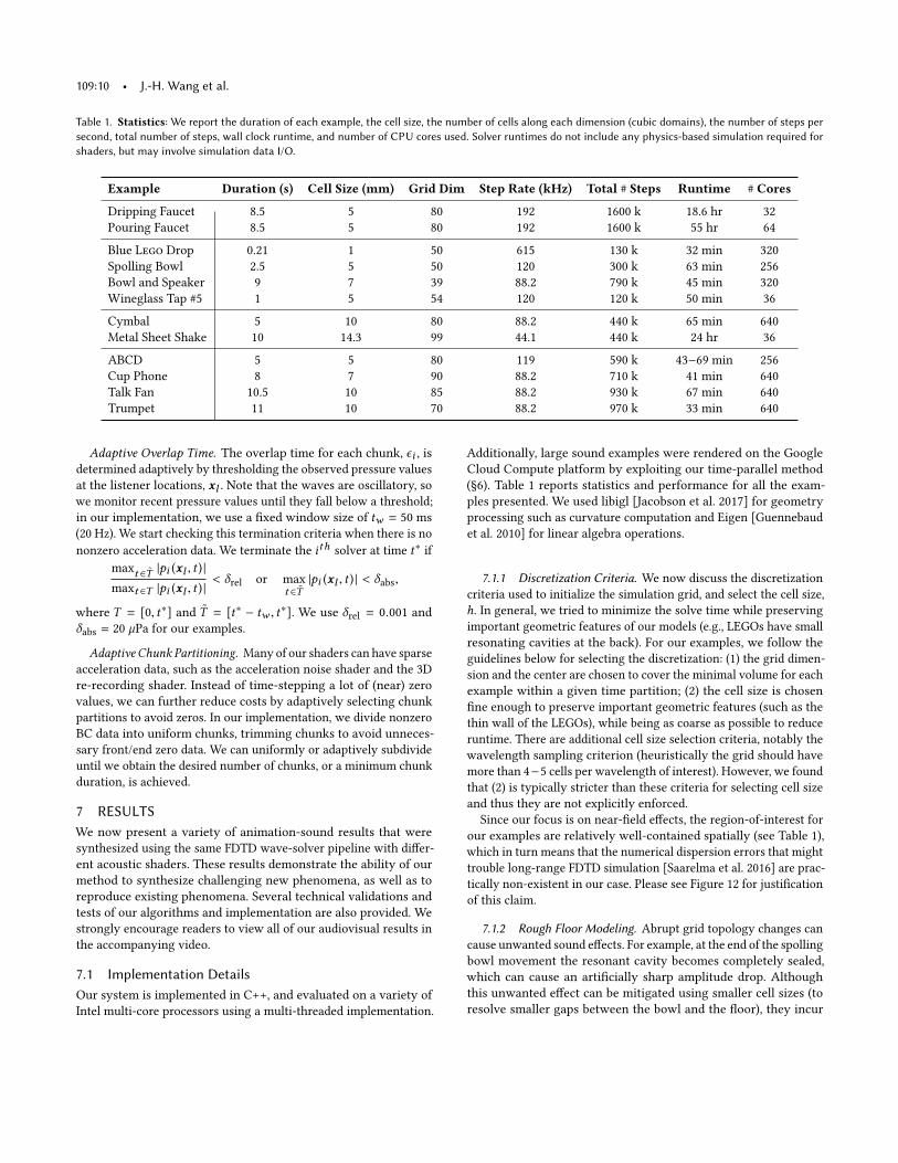
7.1.1 Discretization Criteria. We now discuss the discretization

criteria used to initialize the simulation grid, and select the cell size,

h. In general, we tried to minimize the solve time while preserving

important geometric features of our models (e.g., LEGOs have small

resonating cavities at the back). For our examples, we follow the

guidelines below for selecting the discretization: (1) the grid dimen-

sion and the center are chosen to cover the minimal volume for each

example within a given time partition; (2) the cell size is chosen

ine enough to preserve important geometric features (such as the

thin wall of the LEGOs), while being as coarse as possible to reduce

runtime. There are additional cell size selection criteria, notably the

wavelength sampling criterion (heuristically the grid should have

more than 4−5 cells per wavelength of interest). However, we found

that (2) is typically stricter than these criteria for selecting cell size

and thus they are not explicitly enforced.

Since our focus is on near-ield efects, the region-of-interest for

our examples are relatively well-contained spatially (see Table 1),

which in turn means that the numerical dispersion errors that might

trouble long-range FDTD simulation [Saarelma et al. 2016] are prac-

tically non-existent in our case. Please see Figure 12 for justiication

of this claim.

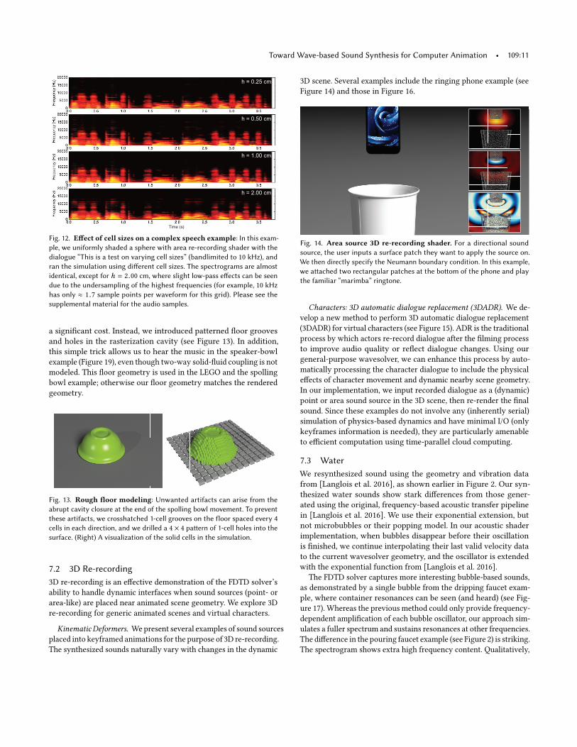
7.1.2 Rough Floor Modeling. Abrupt grid topology changes can

cause unwanted sound efects. For example, at the end of the spolling

bowl movement the resonant cavity becomes completely sealed,

which can cause an artiicially sharp amplitude drop. Although

this unwanted efect can be mitigated using smaller cell sizes (to

resolve smaller gaps between the bowl and the loor), they incur

Toward Wave-based Sound Synthesis for Computer Animation • 109:11

h = 0.25 cm

h = 0.50 cm

h = 1.00 cm

h = 2.00 cm

Time (s)

Fig. 12. Efect of cell sizes on a complex speech example: In this exam-

ple, we uniformly shaded a sphere with area re-recording shader with the

dialogue łThis is a test on varying cell sizesž (bandlimited to 10 kHz), and

ran the simulation using diferent cell sizes. The spectrograms are almost

identical, except for h = 2.00 cm, where slight low-pass efects can be seen

due to the undersampling of the highest frequencies (for example, 10 kHz

has only ≈ 1.7 sample points per waveform for this grid). Please see the

supplemental material for the audio samples.

a signiicant cost. Instead, we introduced patterned loor grooves

and holes in the rasterization cavity (see Figure 13). In addition,

this simple trick allows us to hear the music in the speaker-bowl

example (Figure 19), even though two-way solid-luid coupling is not

modeled. This loor geometry is used in the LEGO and the spolling

bowl example; otherwise our loor geometry matches the rendered

geometry.

Fig. 13. Rough loor modeling: Unwanted artifacts can arise from the

abrupt cavity closure at the end of the spolling bowl movement. To prevent

these artifacts, we crosshatched 1-cell grooves on the floor spaced every 4

cells in each direction, and we drilled a 4 × 4 patern of 1-cell holes into the

surface. (Right) A visualization of the solid cells in the simulation.

7.2 3D Re-recording

3D re-recording is an efective demonstration of the FDTD solver’s

ability to handle dynamic interfaces when sound sources (point- or

area-like) are placed near animated scene geometry. We explore 3D

re-recording for generic animated scenes and virtual characters.

Kinematic Deformers. Wepresent several examples of sound sources

placed into keyframed animations for the purpose of 3D re-recording.

The synthesized sounds naturally vary with changes in the dynamic

3D scene. Several examples include the ringing phone example (see

Figure 14) and those in Figure 16.

Fig. 14. Area source 3D re-recording shader. For a directional sound

source, the user inputs a surface patch they want to apply the source on.

We then directly specify the Neumann boundary condition. In this example,

we atached two rectangular patches at the botom of the phone and play

the familiar łmarimbaž ringtone.

Characters: 3D automatic dialogue replacement (3DADR). We de-

velop a new method to perform 3D automatic dialogue replacement

(3DADR) for virtual characters (see Figure 15). ADR is the traditional

process by which actors re-record dialogue after the ilming process

to improve audio quality or relect dialogue changes. Using our

general-purpose wavesolver, we can enhance this process by auto-

matically processing the character dialogue to include the physical

efects of character movement and dynamic nearby scene geometry.

In our implementation, we input recorded dialogue as a (dynamic)

point or area sound source in the 3D scene, then re-render the inal

sound. Since these examples do not involve any (inherently serial)

simulation of physics-based dynamics and have minimal I/O (only

keyframes information is needed), they are particularly amenable

to eicient computation using time-parallel cloud computing.

7.3 Water

We resynthesized sound using the geometry and vibration data

from [Langlois et al. 2016], as shown earlier in Figure 2. Our syn-

thesized water sounds show stark diferences from those gener-

ated using the original, frequency-based acoustic transfer pipeline

in [Langlois et al. 2016]. We use their exponential extension, but

not microbubbles or their popping model. In our acoustic shader

implementation, when bubbles disappear before their oscillation

is inished, we continue interpolating their last valid velocity data

to the current wavesolver geometry, and the oscillator is extended

with the exponential function from [Langlois et al. 2016].

The FDTD solver captures more interesting bubble-based sounds,

as demonstrated by a single bubble from the dripping faucet exam-

ple, where container resonances can be seen (and heard) (see Fig-

ure 17). Whereas the previous method could only provide frequency-

dependent ampliication of each bubble oscillator, our approach sim-

ulates a fuller spectrum and sustains resonances at other frequencies.

The diference in the pouring faucet example (see Figure 2) is striking.

The spectrogram shows extra high frequency content. Qualitatively,

109:12 • J.-H. Wang et al.

0 1 2 3 4 50

5000

10000

15000

20000

Fre

qu

en

cy (

Hz)

0 1 2 3 4 5

Time

0

5000

10000

15000

20000

Fre

qu

en

cy (

Hz)

A B C D

A B C D

Fig. 15. Application: 3D Automatic Dialogue Replacement (3DADR):

Our system can perform automatic auralization for dialogue placed in 3D

scene. In this example, user specifies a wav file containing a dialogue saying

łA B C Dž (Top row), along with a silent, dynamic 3D scene. By shading

the mouth part of the character with the area source shader, our solver

renders the audio scene and produces a plausible, automatically enhanced

dialogue (Botom row). Corresponding to the visual events, the overall

sound magnitude for łBž (megaphone) is boosted (megaphone), and certain

(resonance) frequencies for łDž (soup pot) are emphasized.

the wavesolver produces a more realistic łwetž sound, compared

to the previous method which essentially played underwater bub-

ble sounds with adjusted amplitudes. Ironically, our wavesolver is

faster than the radiation solves in the previous frequency-domain

approach, because the bubbles’ contributions are amortized to one

wave solve pass.

7.4 Rigid-body Sound

Comparison to łAcoustic Transferž (Wine glass). The frequency-

domain Helmholtz radiation is known to be a good approximation

in certain cases, such as isolated objects in free-space. We compare

impulse responses of a suspended wine glass (see Figure 18) be-

tween our time-domain method and the frequency-domain method

in [Langlois et al. 2014], and obtain very similar impulse responses.

Time-varying acoustic interactions (Spolling Bowl, LEGO). Dy-

namic inter-object interactions cannot be accounted for using the

single-object, precomputedHelmholtz acoustic transfermodel, widely

used in previous work [Zheng and James 2011]. On the contrary,

our method captures several interesting and perceptually impor-

tant near-ield efects such as the time-varying resonance caused

by a spolling bowl on the ground (see Figure 7), or the distinctive

sound that LEGO pieces make when landing on diferent sides (see

Figure 20).

Integratedmulti-shader support (Bowl covering speaker). The acous-

tic shader abstraction provides a natural mechanism for combining

diferent types of shader models. Please see Figure 19 for an exam-

ple that demonstrates the multi-shader support (spolling bowl over

speaker). Simultaneously simulating the 3D re-recording, modal,

and acceleration shaders allows us to capture perceptually important

near-ield acoustic efects.

7.5 Thin Shells

It is straightforward for our system to support dynamic interfaces

arising from unreduced discrete deformable models, e.g., standard

FEM models. To demonstrate this, we synthesized nonlinear thin-

shell sounds from (1) the rapid deformation of crash cymbals after

being hit by a drumstick, and (2) a rectangular metal plate subjected

to large bending and twisting motions (see Figure 21). Spectrogram

analysis shows that these sounds are extremely broadband and

experience complex pitch shifts and spectral cascades throughout

the animation. Previous methods based on linear modal transfer

such as [Chadwick et al. 2009] will most certainly fail under these

extreme cases due to the frequency-localized transfer approximation.

These basic łsheet metalž examples illustrate our system’s ability to

synthesize sound for general large-deformation discrete deformable

models, as opposed to reduced-order modeling [Chadwick et al.

2009]. Readers interested in more detailed, predictive modeling of

cymbals and plates should refer to prior work in the computer music

literature [Bilbao 2009; Chaigne et al. 2005; Ducceschi and Touzé

2015].

8 CONCLUSION AND DISCUSSION

We have explored high-quality oline wave-based sound synthe-

sis for computer animation using a prototype CPU-based FDTD

implementation, with dynamic embedded interfaces and animation-

based acoustic shaders. While the simulations are unoptimized and

expensive, they demonstrate that a rich variety of high-idelity

sound efects, some never before heard, can be generated. Perhaps

the most signiicant improvements are in complex nonlinear phe-

nomena, such as bubble-based water, where no prior methods can

efectively resolve the complex acoustic emissions. Our proposed

parallel-in-time sound-synthesis methods were efective at exposing

additional parallelism for CPU-based cloud computing, and worked

especially well for 3D re-recording examples where data transfer

costs were minimal. We believe this work demonstrates that fu-

ture integrated high-quality animation-sound rendering systems

are indeed plausible, and closer than ever before.

Given the exploratory nature of this work, there are many lessons

learned, many limitations exposed, and many opportunities for fu-

ture work. The most obvious limitation of our approach is that it is

slow. Our CPU-based prototype allowed us to explore the numerical

methods needed to support general animated phenomena, but the

sound system łscreams outž for GPU acceleration, so well leveraged

by prior FDTD sound works [Allen and Raghuvanshi 2015; Webb

2014]. Unique challenges for GPU acceleration here are supporting

dynamic embedded interfaces, and physics-based acoustic shader

implementations and/or data transfer of audio-rate boundary data.

Future pipelines would greatly beneit from simultaneous anima-

tion/sound synthesis, to avoid excessive data storage and transfer.

Parallel-in-time sound methods can greatly improve the paralleliza-

tion of long sound synthesis jobs, such as in feature production,

and are well suited to multi-GPU architectures. They might also

be explored for dynamics to alleviate bottlenecks and data transfer.

Parallel-in-time methods are less efective for short clips, and sound

sources with long reverberation times.

Toward Wave-based Sound Synthesis for Computer Animation • 109:13

Fig. 16. Kinematic Deformers: The objects in all three scenes are kinematically scripted in Blender. They are keyframed and exported to our wavesolver to

perform the 3D re-recording. (Let) The trumpet sound is pre-recorded and is auralized by the bell and the plunger silencer. The amplitude modulation due to

the plunger motion can be clearly heard. (Middle) Speaker behind a rotating fan produces the familiar, funny łroboticž voice. This example also demonstrates

our system is robust under rapid interface movements. (Right) Dipping your phone into a cofee cup while its ringing is not recommended, but it will change

the ringtone quality to include the air resonance of the cup, depending on the height, width, and other cup geometry. These efects are captured naturally

with our solver. Note that slightly simplified geometric models were used to simulate kinematic deformers: only the bell for the trumpet is simulated, and the

outer casing of the fan is neglected (see inset figures for visualization of the rasterization results).

1.75 1.76 1.77 1.78 1.79 1.80 1.81 1.82 1.83 1.75 1.76 1.77 1.78 1.79 1.80 1.81 1.82 1.830

2

7

10

12

-0.2

0.0

0.2

5

Fre

qu

en

cy (

kH

z)

Time (s) Time (s)

Fig. 17. Single Bubble: A single bubble from the dripping faucet. (Let)

Results from [Langlois et al. 2016]. (Right) The same result run through our

wavesolver. Note the extra container resonances excited at 4kHz and 6kHz,

that the previous frequency based method could not capture.

(a) (b)

Fig. 18. Wine glass: Our time-domain method (a) produces similar results

to the widely used frequency-domain Helmholtz radiation method (b) [Lan-

glois et al. 2014] for the isolated wine glass in free-space.

FDTD sound synthesis for animation leads to a host of inter-

related sampling and resolution issues. Low-resolution approxima-

tions can lead to rasterization errors for moving geometry and sound

artifacts. Nonsmooth and under-resolved geometry can cause prob-

lems with the ghost-cell method, including inaccurate BC evaluation

and even, in extreme cases, instabilities. On the other hand, using

iner grids quickly gets costly: cutting spatial resolution by 1/2 in

each dimension also leads to a 1/2 timestep restriction, all of which

increases the cost by 16×. Our prototype uses cubic grids with a

rectangular region-of-interest about each sound source, however

this greatly restricts the motion of the source or can require very

large domains. Future work should investigate adaptive grids, homo-

genenization techniques to resolve multi-scale acoustics problems,

and dynamically sized and moving domains for space-time adap-

tive computations and parallelization. Rapidly moving objects or

under-sampled motions (in sample-and-hold geometry handling)

can necessitate smaller timesteps, e.g., to avoid errors in fresh-cell

classiication which produce sound artifacts. Surface meshes must

be suiciently reined to resolve sound wavelengths of interest (typi-

cally several mm in our examples), however another problem is that

very ine moving geometry can introduce aliasing artifacts when

sampled on a ixed resolution FDTD grid; sampling criteria should

be enforced on input geometry and BCs to ensure that such aliasing

is avoided.

Computer animations can generatemany challenging near-singular

and singular acoustics scenarios. For example, sound passing through

a small opening, or discontinuous changes in the acoustic domain,

e.g., during contact events, can cause a click-like digital sound arti-

fact. Contact events can lead to łclosing voidsž or łpinch ofž events

(e.g., when a bowl lands face down), and łopening voidsž such as

when large air bubbles burst in water animations. Without proper

treatment, even very tiny voids (one to a few cells), which are easily

created and destroyed, can have ill-deined discrete Laplacians for

which null-space-related pressure growth can occur (due to the

unconstrained velocity ield) and, when the void opens, produce

small clicks in extreme cases.

There are many simulation challenges and future work for sound

modeling in animation. Authoring animation-sound results is dii-

cult, and future renderers should leverage modern physics-based

animation tools, like Houdini [Side Efects 2018]. Our framework

uses one-way coupling, i.e., the animation drives the sound, but some

systems, e.g., with enclosed air cavities like a beach ball, require

solid-air coupling to properly resolve sounds. Audio-rate vibration

modeling can be challenging for traditional graphics simulators

not designed to resolve acoustic content; implicit integrators for

deformable models can fail to converge, or produce audible arti-

facts when resorting to adaptive step sizes. Reduced-order vibration

models, such as linear modal models, are traditionally very fast for

sound synthesis, but have unique challenges for FDTD synthesis:

evaluating surface acceleration BCs requires evaluating the modal

transformation every timestep, which can be expensive for larger

109:14 • J.-H. Wang et al.

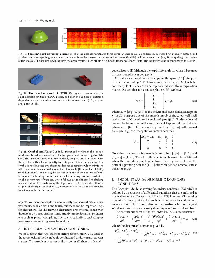
Fig. 19. Spolling Bowl Covering a Speaker: This example demonstrates three simultaneous acoustic shaders: 3D re-recording, modal vibration, and

acceleration noise. Spectrograms of music rendered from the speaker are shown for the case of (Middle) no bowl present, and (Right) the spolling bowl on top

of the speaker. The spolling bowl captures the characteristic pitch-shiting Helmholtz resonance efect. (Note: The input recording is bandlimited to 15 kHz.)

Fig. 20. The familiar sound of LEGO: Our system can resolve the

small acoustic cavities of LEGO pieces, and even the audible orientation-

dependent contact sounds when they land face-down or up (c.f. [Langlois

and James 2014]).

Cymbal

Plate (shake)

Plate (bend)

Cymbal

Fig. 21. Cymbal and Plate: Our fully unreduced nonlinear shell model

results in a broadband sound for both the cymbal and the rectangular plate.

(Top) The drumstick motion is kinematically scripted and it interacts with

the cymbal with a linear penalty force to prevent interpenetration. The

cymbal is held in place by sot spring-damper constraints which mimic the

felt. The cymbal has material parameters identical to [Chadwick et al. 2009].

(Middle/Botom) The rectangular plate is bent and shaken in two diferent

instances. The bending motion is induced by imposing position constraints

on the botom row of vertices, which follows a circular arc. The shaking

motion is done by constraining the top row of vertices, which follows a

scripted shake signal. In both cases, we observe rich spectrum and complex

transients in the output sounds.

objects. We have not explored acoustically transparent and absorp-

tive media, such as cloth and fabric, but these can be important, e.g.,

for characters. Rapidly moving characters present challenges with

diverse body poses and motions, and dynamic domains. Phenom-

ena such as paper crumpling, fracture, vocalization, and complex

machinery are exciting areas to explore.

A INTERPOLATION MATRIX CONDITIONING

We now show that the trilinear interpolation matrix, Φ, used in

the ghost-cell method can be ill-conditioned under certain circum-

stances. This problem is easier to illustrate in 2D than in 3D, and it

generalizes to 3D (although the explicit formula for when it becomes

ill-conditioned is less compact).

Consider a canonical cube C occupying the space [0, 1]3. Suppose

there are some data p ∈ R4 deined over the vertices of C. The trilin-

ear interpolant inside C can be represented with the interpolation

matrix, Φ, such that for some weights c ∈ R4, we have

Φc =

ϕ1

ϕ2

ϕ3

ϕ4

c = p, (21)

whereϕi = [xiyi xi yi 1] is the polynomial basis evaluated at point

xi in 2D. Suppose one of the stencils involves the ghost-cell itself

and a row of Φ needs to be replaced (see ğ3.2). Without loss of

generality, let us assume the replacement happens at the irst row,

where x1 = [0, 0]. For a boundary point xb = [x ,y] with normal

nb = [nx ,ny ], the interpolation matrix becomes

Φ =

xny + ynx nx ny 0

0 1 0 1

1 1 1 1

0 0 1 1

(22)

Note that this matrix is rank-deicient when [x ,y] = [0, 0], and

[nx ,ny ] = [1,−1]. Therefore, the matrix can become ill-conditioned

when the boundary point gets closer to the ghost cell, and the

normal is pointing near the [1,−1] direction. We can observe similar

behavior in 3D.

B ENGQUIST-MAJDA ABSORBING BOUNDARYCONDITIONS

The Engquist-Majda absorbing boundary condition (EM-ABC) is

deined by a sequence of diferential equations that are enforced at

the grid boundary [Engquist and Majda 1977] in order of increasing

numerical accuracy. Since the problem is symmetric in all directions,

we only derive the discretization at the positive x face of the grid.

We also assume no air viscosity damping α = 0 in this derivation.

The continuous form of the 2nd-order EM-ABCs are written as

∂2p (x , t )

∂t2+ c∂p (x , t )

∂x∂t−c2

2

(

∂2p (x , t )

∂y2+

∂2p (x , t )

∂z2

)

= 0, (23)

where the discretized version is given by

pn+1i, j,k+ pn−1

i, j,k− 2pn

i, j,k

τ 2+

c

2h(pni+1, j,k − p

n−1i+1, j,k − p

ni−1, j,k + p

n−1i−1, j,k ) (24)

−c2

2h2(pni, j+1,k + p

ni, j−1,k + p

ni, j,k+1 + p

ni, j,k−1 − 4p

ni, j,k ) = 0.

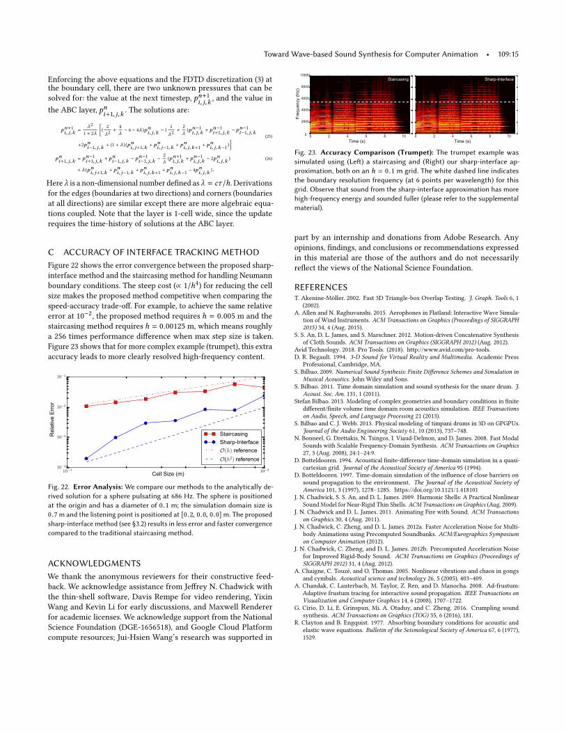
Toward Wave-based Sound Synthesis for Computer Animation • 109:15

Enforcing the above equations and the FDTD discretization (3) atthe boundary cell, there are two unknown pressures that can besolved for: the value at the next timestep, pn+1

i, j,k, and the value in

the ABC layer, pni+1, j,k

. The solutions are:

pn+1i, j,k

=

λ2

1 + 2λ

[(2

λ2+

4

λ− 6 − 4λ )pn

i, j,k− (

1

λ2+

2

λ)pn−1i, j,k

+ pn−1i+1, j,k

− pn−1i−1, j,k

+2pni−1, j,k

+ (1 + λ ) (pni, j+1,k

+ pni, j−1,k

+ pni, j,k+1

+ pni, j,k−1

)

] (25)

pni+1, j,k

= pn−1i+1, j,k

+ pni−1, j,k

− pn−1i−1, j,k

−2

λ(pn+1i, j,k

+ pn−1i, j,k

− 2pni, j,k

) (26)

+ λ (pni, j+1,k

+ pni, j−1,k

+ pni, j,k+1

+ pni, j,k−1

− 4pni, j,k

) .

Here λ is a non-dimensional number deined as λ = cτ/h. Derivations

for the edges (boundaries at two directions) and corners (boundaries

at all directions) are similar except there are more algebraic equa-

tions coupled. Note that the layer is 1-cell wide, since the update

requires the time-history of solutions at the ABC layer.

C ACCURACY OF INTERFACE TRACKING METHOD

Figure 22 shows the error convergence between the proposed sharp-

interface method and the staircasing method for handling Neumann

boundary conditions. The steep cost (∝ 1/h4) for reducing the cell

size makes the proposed method competitive when comparing the

speed-accuracy trade-of. For example, to achieve the same relative

error at 10−2, the proposed method requires h = 0.005 m and the

staircasing method requires h = 0.00125 m, which means roughly

a 256 times performance diference when max step size is taken.

Figure 23 shows that for more complex example (trumpet), this extra

accuracy leads to more clearly resolved high-frequency content.

10−3 10−2

Cell Size (m)

10−4

10−3

10−2

10−1

RelativeError

Staircasing

Sharp-Interface

O(h) reference

O(h2) reference

Fig. 22. Error Analysis:We compare our methods to the analytically de-

rived solution for a sphere pulsating at 686 Hz. The sphere is positioned

at the origin and has a diameter of 0.1 m; the simulation domain size is

0.7m and the listening point is positioned at [0.2, 0.0, 0.0]m. The proposed

sharp-interface method (see ğ3.2) results in less error and faster convergence

compared to the traditional staircasing method.

ACKNOWLEDGMENTS

We thank the anonymous reviewers for their constructive feed-

back. We acknowledge assistance from Jefrey N. Chadwick with

the thin-shell software, Davis Rempe for video rendering, Yixin

Wang and Kevin Li for early discussions, and Maxwell Renderer

for academic licenses. We acknowledge support from the National

Science Foundation (DGE-1656518), and Google Cloud Platform

compute resources; Jui-Hsien Wang’s research was supported in

0 2 4 6 8 100

2000

4000

6000

8000

10000

Fre

qu

en

cy (

Hz)

Time (s) Time (s)

0 2 4 6 8 10

Staircasing Sharp-Interface

Fig. 23. Accuracy Comparison (Trumpet): The trumpet example was

simulated using (Let) a staircasing and (Right) our sharp-interface ap-

proximation, both on an h = 0.1 m grid. The white dashed line indicates

the boundary resolution frequency (at 6 points per wavelength) for this

grid. Observe that sound from the sharp-interface approximation has more

high-frequency energy and sounded fuller (please refer to the supplemental

material).

part by an internship and donations from Adobe Research. Any

opinions, indings, and conclusions or recommendations expressed

in this material are those of the authors and do not necessarily

relect the views of the National Science Foundation.

REFERENCEST. Akenine-Möller. 2002. Fast 3D Triangle-box Overlap Testing. J. Graph. Tools 6, 1

(2002).A. Allen and N. Raghuvanshi. 2015. Aerophones in Flatland: Interactive Wave Simula-

tion of Wind Instruments. ACM Transactions on Graphics (Proceedings of SIGGRAPH2015) 34, 4 (Aug. 2015).

S. S. An, D. L. James, and S. Marschner. 2012. Motion-driven Concatenative Synthesisof Cloth Sounds. ACM Transactions on Graphics (SIGGRAPH 2012) (Aug. 2012).

Avid Technology. 2018. Pro Tools. (2018). http://www.avid.com/pro-tools.D. R. Begault. 1994. 3-D Sound for Virtual Reality and Multimedia. Academic Press

Professional, Cambridge, MA.S. Bilbao. 2009. Numerical Sound Synthesis: Finite Diference Schemes and Simulation in

Musical Acoustics. John Wiley and Sons.S. Bilbao. 2011. Time domain simulation and sound synthesis for the snare drum. J.

Acoust. Soc. Am. 131, 1 (2011).Stefan Bilbao. 2013. Modeling of complex geometries and boundary conditions in inite

diferent/inite volume time domain room acoustics simulation. IEEE Transactionson Audio, Speech, and Language Processing 21 (2013).

S. Bilbao and C. J. Webb. 2013. Physical modeling of timpani drums in 3D on GPGPUs.Journal of the Audio Engineering Society 61, 10 (2013), 737ś748.

N. Bonneel, G. Drettakis, N. Tsingos, I. Viaud-Delmon, and D. James. 2008. Fast ModalSounds with Scalable Frequency-Domain Synthesis. ACM Transactions on Graphics27, 3 (Aug. 2008), 24:1ś24:9.

D. Botteldooren. 1994. Acoustical inite-diference time-domain simulation in a quasi-cartesian grid. Journal of the Acoustical Society of America 95 (1994).

D. Botteldooren. 1997. Time-domain simulation of the inluence of close barriers onsound propagation to the environment. The Journal of the Acoustical Society ofAmerica 101, 3 (1997), 1278ś1285. https://doi.org/10.1121/1.418101

J. N. Chadwick, S. S. An, and D. L. James. 2009. Harmonic Shells: A Practical NonlinearSound Model for Near-Rigid Thin Shells. ACM Transactions on Graphics (Aug. 2009).

J. N. Chadwick and D. L. James. 2011. Animating Fire with Sound. ACM Transactionson Graphics 30, 4 (Aug. 2011).

J. N. Chadwick, C. Zheng, and D. L. James. 2012a. Faster Acceleration Noise for Multi-body Animations using Precomputed Soundbanks. ACM/Eurographics Symposiumon Computer Animation (2012).

J. N. Chadwick, C. Zheng, and D. L. James. 2012b. Precomputed Acceleration Noisefor Improved Rigid-Body Sound. ACM Transactions on Graphics (Proceedings ofSIGGRAPH 2012) 31, 4 (Aug. 2012).

A. Chaigne, C. Touzé, and O. Thomas. 2005. Nonlinear vibrations and chaos in gongsand cymbals. Acoustical science and technology 26, 5 (2005), 403ś409.

A. Chandak, C. Lauterbach, M. Taylor, Z. Ren, and D. Manocha. 2008. Ad-frustum:Adaptive frustum tracing for interactive sound propagation. IEEE Transactions onVisualization and Computer Graphics 14, 6 (2008), 1707ś1722.

G. Cirio, D. Li, E. Grinspun, Mi. A. Otaduy, and C. Zheng. 2016. Crumpling soundsynthesis. ACM Transactions on Graphics (TOG) 35, 6 (2016), 181.

R. Clayton and B. Engquist. 1977. Absorbing boundary conditions for acoustic andelastic wave equations. Bulletin of the Seismological Society of America 67, 6 (1977),1529.

109:16 • J.-H. Wang et al.

M. Cook. 2015. Pixar, ’The Road to Point Reyes’ and the long history of landscape innew visual technologies. (2015).

P. R. Cook. 2002. Sound Production and Modeling. IEEE Computer Graphics & Applica-tions 22, 4 (July/Aug. 2002), 23ś27.

R. L. Cook, L. Carpenter, and E. Catmull. 1987. The Reyes Image Rendering Architecture.In Proceedings of the 14th Annual Conference on Computer Graphics and InteractiveTechniques (SIGGRAPH ’87). ACM, New York, NY, USA, 95ś102. https://doi.org/10.1145/37401.37414

M. Ducceschi and C. Touzé. 2015. Modal approach for nonlinear vibrations of dampedimpacted plates: Application to sound synthesis of gongs and cymbals. Journal ofSound and Vibration 344 (2015), 313ś331.

B. Engquist and A. Majda. 1977. Absorbing boundary conditions for numerical sim-ulation of waves. Proceedings of the National Academy of Sciences 74, 5 (1977),1765ś1766.

Ronald P Fedkiw, Tariq Aslam, Barry Merriman, and Stanley Osher. 1999. A Non-oscillatory Eulerian Approach to Interfaces in Multimaterial Flows (the Ghost FluidMethod). J. Comput. Phys. 152, 2 (1999), 457 ś 492.

T. Funkhouser, I. Carlbom, G. Elko, G. Pingali, M. Sondhi, and J. West. 1998. A BeamTracing Approach to Acoustic Modeling for Interactive Virtual Environments. InProceedings of SIGGRAPH 98 (Computer Graphics Proceedings, Annual ConferenceSeries). 21ś32.

T. A. Funkhouser, P. Min, and I. Carlbom. 1999. Real-Time Acoustic Modeling for Dis-tributed Virtual Environments. In Proceedings of SIGGRAPH 99 (Computer GraphicsProceedings, Annual Conference Series). 365ś374.

W. W. Gaver. 1993. Synthesizing auditory icons. In Proceedings of the INTERACT’93 andCHI’93 conference on Human factors in computing systems. ACM, 228ś235.

Y. I. Gingold, A. Secord, J. Y. Han, E. Grinspun, and D. Zorin. 2004. A Discrete Modelfor Inelastic Deformation of Thin Shells.

G. Guennebaud, B. Jacob, et al. 2010. Eigen v3. http://eigen.tuxfamily.org. (2010).Jon Häggblad and Björn Engquist. 2012. Consistent modeling of boundaries in acoustic

inite-diference Time-domain simulations. Journal of the Acoustical Society ofAmerica 132 (2012).

P. S. Heckbert. 1987. Ray tracing Jell-O brand gelatin. In ACM SIGGRAPH ComputerGraphics, Vol. 21. ACM, 73ś74.

A. Jacobson, D. Panozzo, et al. 2017. libigl: A simple C++ geometry processing library.(2017). http://libigl.github.io/libigl/.

D. L. James, J. Barbic, and D. K. Pai. 2006. Precomputed Acoustic Transfer: Output-sensitive, accurate sound generation for geometrically complex vibration sources.ACM Transactions on Graphics 25, 3 (July 2006), 987ś995.

D. L. James and D. K. Pai. 2002. DyRT: Dynamic Response Textures for Real TimeDeformation Simulation with Graphics Hardware. ACM Trans. Graph. 21, 3 (July2002), 582ś585. https://doi.org/10.1145/566654.566621

M. Kleiner, B.-I. Dalenbäck, and P. Svensson. 1993. AuralizationśAn Overview. J. AudioEngineering Society 41 (1993), 861ś861. Issue 11.

D. Komatitsch, G. Erlebacher, D. Göddeke, and D. Michéa. 2010. High-order inite-element seismic wave propagation modeling with MPI on a large GPU cluster.Journal of computational physics 229, 20 (2010), 7692ś7714.

T. R. Langlois, S. S. An, K. K. Jin, and D. L. James. 2014. Eigenmode Compressionfor Modal Sound Models. ACM Trans. Graph. 33, 4, Article 40 (July 2014), 9 pages.https://doi.org/10.1145/2601097.2601177

T. R Langlois and D. L James. 2014. Inverse-foley animation: Synchronizing rigid-bodymotions to sound. ACM Transactions on Graphics (TOG) 33, 4 (2014), 41.

T. R. Langlois, C. Zheng, and D. L. James. 2016. Toward Animating Water with ComplexAcoustic Bubbles. ACM Trans. Graph. 35, 4, Article 95 (July 2016), 13 pages. https://doi.org/10.1145/2897824.2925904

S. Larsson and V. Thomée. 2009. Partial Diferential Equations with Numerical Methods.Springer.

Q.-H. Liu and J. Tao. 1997. The perfectly matched layer for acoustic waves in absorptivemedia. The Journal of the Acoustical Society of America 102, 4 (1997), 2072ś2082.

S. Marburg and B. Nolte. 2008. Computational acoustics of noise propagation in luids:inite and boundary element methods. Vol. 578. Springer.

R. Mehra, N. Raghuvanshi, L. Antani, A. Chandak, S. Curtis, and D. Manocha. 2013.Wave-based sound propagation in large open scenes using an equivalent sourceformulation. ACM Transactions on Graphics (TOG) 32, 2 (2013), 19.

R. Mehra, N. Raghuvanshi, L. Savioja, M. C. Lin, and D. Manocha. 2012. An eicientGPU-based time domain solver for the acoustic wave equation. Applied Acoustics73, 2 (2012), 83 ś 94.

A. Meshram, R. Mehra, H. Yang, E. Dunn, J.-M. Frahm, and D. Manochak. 2014. P-hrtf:Eicient personalized hrtf computation for high-idelity spatial sound. Mixed andAugmented Reality (ISMAR), 2014 IEEE International Symposium on (2014).

P. Micikevicius. 2009. 3D Finite Diference Computation on GPUs Using CUDA. InProceedings of 2Nd Workshop on General Purpose Processing on Graphics ProcessingUnits (GPGPU-2). ACM, New York, NY, USA, 79ś84. https://doi.org/10.1145/1513895.1513905

M. Minnaert. 1933. XVI. On musical air-bubbles and the sounds of running water. TheLondon, Edinburgh, and Dublin Philosophical Magazine and Journal of Science 16, 104

(1933), 235ś248.R. Mittal, H. Dong, M. Bozkurttas, F. M. Najjar, A. Vargas, and A. Loebbecke. 2008. A

versatile sharp interface immersed boundary method for incompressible lows withcomplex boundaries. J. Comput. Phys. 227 (2008).

R. Mittal and G. Iaccarino. 2005. Immersed Boundary Methods. Annual Review of FluidMechanics 37 (2005).

P. Morse and K. U. Ingard. 1968. Theoretical Acoustics. Princeton University Press,Princeton, New Jersey.

W. Moss, H. Yeh, J.-M. Hong, M. C. Lin, and D. Manocha. 2010. Sounding Liquids:Automatic Sound Synthesis from Fluid Simulation. ACM Trans. Graph. 29, 3 (2010).

J. F. O’Brien, P. R. Cook, and G. Essl. 2001. Synthesizing Sounds From Physically BasedMotion. In Proceedings of SIGGRAPH 2001. 529ś536.

J. F. O’Brien, C. Shen, and C. M. Gatchalian. 2002. Synthesizing sounds from rigid-bodysimulations. In The ACM SIGGRAPH 2002 Symposium on Computer Animation. ACMPress, 175ś181.

C. S. Peskin. 1981. The luid dynamics of heart valves: experimental, theoretical andcomputational methods. Annual Review of Fluid Mechanics 14 (1981).

N. Raghuvanshi, R. Narain, and M. C. Lin. 2009. Eicient and Accurate Sound Propaga-tion Using Adaptive Rectangular Decomposition. IEEE Trans. Vis. Comput. Graph.15, 5 (2009), 789ś801. https://doi.org/10.1109/TVCG.2009.28

N. Raghuvanshi and J. Snyder. 2014. Parametric wave ield coding for precomputedsound propagation. ACM Transactions on Graphics (TOG) 33, 4 (2014), 38.

J. Saarelma, J. Botts, B. Hamilton, and L. Savioja. 2016. Audibility of dispersion error inroom acoustic inite-diference time-domain simulation as a function of simulationdistance. The Journal of the Acoustical Society of America 139, 4 (2016), 1822ś1832.

C. Schissler, R. Mehra, and D. Manocha. 2014. High-order difraction and difuse relec-tions for interactive sound propagation in large environments. ACM Transactionson Graphics (TOG) 33, 4 (2014), 39.

C. Schreck, D. Rohmer, D. James, S. Hahmann, and M.-P. Cani. 2016. Real-time soundsynthesis for paper material based on geometric analysis. In Eurographics/ACMSIGGRAPH Symposium on Computer Animation (2016).

E. Schweickart, D. L. James, and S. Marschner. 2017. Animating Elastic Rods with Sound.ACM Transactions on Graphics 36, 4 (July 2017). https://doi.org/10.1145/3072959.3073680

A. A. Shabana. 2012. Theory of Vibration: An Introduction. Springer Science & BusinessMedia.

A. A. Shabana. 2013. Dynamics of multibody systems. Cambridge university press.Side Efects. 2018. Houdini Engine. (2018). http://www.sidefx.com.J. O. Smith. 1992. Physical modeling using digital waveguides. Computer music journal

16, 4 (1992), 74ś91.A. Talove and S. C. Hagness. 2005. Computational Electrodynamics: The Finite-Diference

Time-Domain Method. Artech House.T. Takala and J. Hahn. 1992. Sound rendering. In Computer Graphics (Proceedings of

SIGGRAPH 92). 211ś220.J. G. Tolan and J. B. Schneider. 2003. Locally conformal method for acoustic inite-

diference time-domain modeling of rigid surfaces. Journal of the Acoustical Societyof America 114 (2003).

N. Tsingos, T. Funkhouser, A. Ngan, and I. Carlbom. 2001. Modeling acoustics in virtualenvironments using the uniform theory of difraction. In SIGGRAPH ’01: Proceedingsof the 28th annual conference on Computer graphics and interactive techniques. ACM,New York, NY, USA, 545ś552.

K. van den Doel. 2005. Physically Based Models for Liquid Sounds. ACM Trans. Appl.Percept. 2, 4 (Oct. 2005), 534ś546. https://doi.org/10.1145/1101530.1101554

K. van den Doel, P. G. Kry, and D. K. Pai. 2001. FoleyAutomatic: Physically-basedSound Efects for Interactive Simulation and Animation. (2001), 537ś544. https://doi.org/10.1145/383259.383322

K. van den Doel and D. K. Pai. 1998. The sounds of physical shapes. Presence: Teleoper-ators and Virtual Environments 7, 4 (1998), 382ś395.

M. Vorländer. 2008. Auralization. Aachen: Springer (2008).C. J. Webb. 2014. Parallel computation techniques for virtual acoustics and physical

modelling synthesis. Ph.D. Dissertation.C. J. Webb and S. Bilbao. 2011. Computing room acoustics with CUDA - 3D FDTD

schemes with boundary losses and viscosity. 2011 IEEE International Conference onAcoustics, Speech and Signal Processing (ICASSP) (2011), 317ś320.

H. Yeh, R. Mehra, Z. Ren, L. Antani, D. Manocha, and M. Lin. 2013. Wave-ray Couplingfor Interactive Sound Propagation in Large Complex Scenes. ACM Trans. Graph. 32,6, Article 165 (Nov. 2013), 11 pages. https://doi.org/10.1145/2508363.2508420

C. Zheng and D. L. James. 2009. Harmonic Fluids. ACM Transactions on Graphics(SIGGRAPH 2009) 28, 3 (Aug. 2009).

C. Zheng and D. L. James. 2010. Rigid-Body Fracture Sound with Precomputed Sound-banks. ACM Transactions on Graphics (SIGGRAPH 2010) 29, 3 (July 2010).

C. Zheng and D. L. James. 2011. Toward High-Quality Modal Contact Sound. ACMTransactions on Graphics (Proceedings of SIGGRAPH 2011) 30, 4 (Aug. 2011).