Toward an Understanding of Learning by Doing:

Evidence from an Automobile Assembly Plant∗

Steven D. Levitt Univ. of Chicago and NBER

slevitt@uchicago.edu

John A. List Univ. of Chicago and NBER

jlist@uchicago.edu

Chad Syverson Univ. of Chicago Booth School of

Business and NBER chad.syverson@chicagobooth.edu

April 2013

Abstract We use detailed data from an assembly plant of a major auto producer to investigate the learning by doing process. We focus on the acquisition, aggregation, transmission, and embodiment of the knowledge stock built through learning. We find that most of the substantial learning by doing knowledge at the plant was not retained by the plant’s workers, even though they were an important conduit for knowledge acquisition. This finding is consistent with the plant’s institutionalized systems for productivity measurement and improvement. We further explore how overall learning is undergirded by what happens at the hundreds of individual processes along the production line. Our results shed light not only on how productivity gains accrue at the plant level, but also how firms apply managerial inputs to expand production.

∗ We received generous help from numerous individuals at the auto manufacturer from which our data are obtained, but we would especially like to thank Rich D., Shannon A., and Robert M. In particular, Marco O. was an invaluable resource in helping us understand details of the production process and the associated data infrastructure. We also thank Francis Kramarz and seminar participants at Chicago, Columbia, Minnesota, Toronto Rotman, and the ZEW IT conference for helpful comments. We are grateful to David Greis, Kris Hult, Maria Ibanez, Carter Mundell, Dhiren Patki, and Laura Rivera for their extensive research assistance. Contact information: Levitt and List: University of Chicago Department of Economics, 1126 E. 59th St., Chicago, IL, 60637; Syverson (corresponding author): University of Chicago Booth School of Business, 5807 S. Woodlawn Ave., Chicago, IL 60637.

1

I. Introduction

Learning by doing has occupied a central place within economics ever since Arrow

(1962) used the concept as a workhorse in his theory of endogenous growth. Arrow

conceptualized learning by doing within the actual activity of production, with cumulative gross

investment as the catalyst for experience. Nearly two decades later, the role of experience in

shaping and driving productivity growth was central in Lucas’ (1988) explanations of increasing

returns to human capital. Indeed, Lucas (1988, p. 27) argues “on-the-job-training or learning by

doing appear to be at least as important as schooling in the formation of human capital.” Yang

and Borland (1991) furthered this line of thought by theoretically linking the division of labor

and learning by doing, highlighting an important source of comparative advantage.

Empirical studies have confirmed the importance of learning by doing in practice.

Scholars have frequently observed that improvements in the efficiency with which outputs are

produced from existing technologies and inputs are an important source of total factor

productivity (TFP) growth. One early example was described in Lundberg (1961), who describes

the experience of the Horndal iron works plant in Sweden. Although the plant had no new

investment over a period of 15 years, output per worker hour rose about 2 percent annually.

Another stark early observation of such progress was in the aircraft industry. As Wright (1936)

and Middleton (1945) note, labor inputs per airframe declined considerably as the total number

of airframes produced increased. Progress of this sort has been found across scores of studies,

often attributed to adaptation efforts by labor, and argued to occur independently of scale effects.

In this paper, we harness rich data from an assembly plant of a major automaker to

address open questions about how the knowledge built through learning by doing is acquired,

aggregated, diffused, and embodied. Our core data set covers in incredible detail the production

of about 190,000 cars over the course of a production year. The year was full of potential

learning opportunities, as the firm had both redesigned the cars made at the plant and introduced

a new production process into the plant. We observe, for each vehicle the plant assembles,

several hundred individual operations on the assembly line. We see the specific time at which

each of these operations takes place and any problems that arise with the operation, allowing us

to compute the rate at which production problems (defects) occur, either car-by-car or over

aggregated time periods.

2

Our analysis reveals a number of interesting findings. Consonant with previous learning

by doing studies, we find that the auto assembly plant quickly realized large efficiency gains in

both the quality and quantity dimensions. Both assembly defects per vehicle and the average

number of hours required to assemble a car dropped by about 70 percent during the first eight

weeks of production. These quality gains in particular, which are rarely measured in the

literature, are further verified in two additional data sets: quality audits performed on randomly

selected vehicles and initial warranty claims by buyers of the cars made at the plant.

When we track the transmission and embodiment of learning by doing knowledge, we

find that, interestingly, despite the substantial learning these early productivity improvements

represent, the plant’s second shift was able to come on line in the eighth week of production and

immediately operate at the first shift’s contemporaneous quality performance. Further tying the

performance of the shifts together, we document that the hundreds of processes involved in

assembling a car had highly correlated defect rates across shifts within the same time period. In

other words, most defect-prone processes on one shift tended to be the most defect-prone

processes on the other, even though the workers completing these tasks were different.

These across-shift patterns stand in contrast with what we observe when production of a

new model variant ramped up at the plant, as happened twice later in the year. In those cases, the

learning process started again; production of the new variant initially exhibited much higher

defect rates than the variant(s) already being produced. We also test whether worker absenteeism

was related to defect rates. We find that it was, but that the impact was economically small.

These results in combination indicate that, in terms of knowledge transition and embodiment,

most of the substantial learning by doing at the plant was not retained by the plant’s workers,

even though they were an important conduit for knowledge acquisition. This is consistent with

the operation of the plant’s institutionalized systems for productivity measurement and

improvement, and in particular a whiteboard system that encourages line workers to report

production problems that management can address. We describe these systems in detail in the

next section.

In sum, we find considerable evidence of learning by doing in quality and quantity

productivity performance, particularly early in the production year. Yet the second set of

results—the immediate performance of the new shift, the correlation in contemporaneous defect

rates across shifts, the contrast of these across-shift patterns with the re-learning that occurs

3

when production of a new model variant begins, and the small effect of absenteeism—indicate

that most of the knowledge stock built by learning does not stay with the plant’s line workers.

Instead, it quickly becomes embodied in the physical or broader organizational capital of the

plant.

Our findings add new insights to a literature that has been attempting to move beyond a

progress function that simply relates reductions in unit costs to cumulative production. One

distinction of this study is our unusual ability to look at learning as reflected in quality-based

productivity outcomes.1 A second distinction is our focus on the nature of the knowledge stock

built through learning by doing. Much of the economic research on learning by doing in specific

production settings has focused on measuring the overall dynamics of the learning process—for

example, how fast productivity gains accrue or whether measured learning rates imply that

knowledge might be “forgotten” over time. More recent work, along with a separate operations

management literature on learning by doing, has sought to go beyond characterizations of

learning curves as mechanical processes driven by production experience. These studies have

explored how producers’ organizational structures and decisions interact with and affect the

ways in which learning occurs.2

1 To our knowledge, no other learning by doing studies in the economics literature has focused on productivity as reflected in output quality rather than some measure of output quantity. We are aware of one learning by doing study in the operations management literature that uses quality as an outcome, Levin (2000). That article investigates auto quality too, but rather in its evolution from one model year to the next over a model’s design lifecycle (as reflected in Consumer Reports ratings). As we discuss below, the quality changes we observe within the single model year of our sample are an order of magnitude larger than those we observe across model years. We do also document learning patterns in quantity productivity metrics below, which allow us to make what are as far as we know the first side-by-side quantitative comparisons of quality- and quantity-based productivity gains from learning by doing.

But this work has revealed less—largely because of data

limitations—about the nature of the knowledge stock that is built through learning by doing. In

particular, there remain many open questions about the specifics of how production knowledge is

acquired, aggregated, and transmitted throughout complex production operations, and where and

how this knowledge stock is eventually embodied in inputs. We address these questions by

2 The relevant literature is too large to cite fully. Some examples of more recent work include Malerba (1992); Jarmin (1994); Darr, Argote, and Epple (1995); Jovanovic and Nyarko (1995); von Hippel and Tyre (1995); Epple, Argote, and Murphy (1996); Hatch and Mowery (1998); Benkard (2000); Levin (2000); Sinclair, Klepper, and Cohen (2000); Thompson (2001); Thornton and Thompson (2001); Schilling et al. (2003); Thompson (2007); and Hendel and Spiegel (2012). Argote and Epple (1990) and Thompson (2010, 2012) offer surveys. A related yet distinct line of economic research has used detailed production data to do “insider econometrics” (Ichniowski and Shaw (2012)) and explore how various factors like incentive pay, human resources policies, and management practices affect a firm’s productivity. Examples include Lazear (2000), Hamilton et al. (2003), Krueger and Mas (2004), Bandiera et al. (2007, 2009), Hossain and List (2012), Bloom et al. (2013), and Das et al. (2013).

4

combining evidence on the transfer of learning across shifts (Epple, Argote and Murphy (1996))

with evidence on the transfer of learning across model varieties. Across-variant transfer patterns

exhibit fundamental differences from across-shift transfers, offering insights into the particular

ways in which the learning by doing knowledge stock is acquired, transmitted, and embodied. A

further way our study adds to the literature is our ability to observe production at a highly

disaggregated—that is, process-by-process—level. We use this to further test the nature of

knowledge transfer and embodiment and, in the online appendix, to characterize the nature of the

process-level defect rate distribution that underlies the aggregate (car-level) productivity

numbers that are our focus.

By fleshing out several details of the learning by doing process in an important industry,

we learn more about the nature of the production knowledge stock itself. In this broader, more

full-fledged view of learning by doing, a producer’s experience gains do not so much cause

efficiency enhancements themselves as they provide opportunities for management to exploit

(Dutton and Thomas (1984)). Knowing more about such opportunities starts us on a path to

better understand how specific productivity gains accrue at the plant level and how firms might

optimally expand production. In addition, it provides some empirical content suggesting how

comparative advantage arises, and what leads to specialization.

The remainder of the paper is structured as follows. Section II describes the production

setting from which our data are drawn. Section III overviews the data. Sections IV and V present

empirical results that, respectively, document the basic learning by doing patterns at the plant

and explore the transmission and embodiment of the learning knowledge stock. A final section

discusses implications of our empirical results.

II. The Production Setting

Our production data are from an assembly plant of a major automaker. Assembly plants

are factories that piece together the thousands of parts that make up an automobile for delivery to

final customers, either directly to fleet buyers such as car rental companies or indirectly through

retail dealerships.3

3 The extent to which assembly plants are vertically integrated backward into making the parts they assemble varies somewhat across the industry, though there has been a general trend to move more parts fabrication offsite. Our

Non-assembly operations in the plant mostly involve conducting an

assortment of quality-control tests of finished vehicles.

5

A. Plant Operations during the Sample Model Year

Our sample is from the first year of operations following a substantial reorganization of

the plant’s production. This involved major redesigns in the vehicles assembled at the plant,

changes in the assembly line’s physical layout, and a shift into team-based production.4

These changes mean that, in many ways, the plant and its workers were starting over, or

what the literature refers to as entering the ‘ramping up’ process: they were making new products

in a new way. This provides us with a unique glimpse of the learning by doing process, since as

has typically been found in other studies, learning is nonlinear: large gains are realized quickly,

but the speed of progress slows over time. Therefore we are likely to observe considerably larger

changes in defect rates than if we were to follow production of a product the plant had already

been making for some time.

Team

production dispenses with the traditional assembly line practice of having individual workers

hold responsibility for a particular task on the line. Instead, a team of typically 5-6 workers is

jointly responsible for a set of related tasks. Team members rotate through these tasks during the

day and help their teammates when needed. One worker (a line worker not considered as

management within the plant’s hierarchy) is designated as a team leader. This worker is paid a

small wage premium and has particular responsibilities involving oversight, training, and

information aggregation.

5

particular plant reflects that movement; engines are brought into the plant ready to install from a separate factory, for example. Body panels are also struck at a separate though geographically close stamping plant.

The high learning rate over our sample permits us to observe

details of the learning process with greater resolution than would be possible later in the product

design cycle, improving our ability to study the details of the learning by doing process. Another

distinct advantage of examining data during the ramp up stage relates to shrinking product life

cycles. As the lifespan of manufactured goods has decreased, especially among high-tech

products, ramp up events have become more common. Understanding the factors influencing the

4 While new capital and tooling were put in place before the start of the production year, the quantity of the plant’s physical capital inputs was essentially fixed over the production year, reducing concerns that the addition of unobserved inputs creates spurious learning by doing productivity patterns (Thompson (2001)). 5 This is confirmed in our case. Defect rates were much lower in the model previous to our sample. For example, quality audit scores (we describe the audits and the scoring system in detail below) in the prior production year had been basically flat a year and were an order of magnitude smaller than their levels at the beginning of our sample. These earlier models had been made for over six years at the plant, and as such most of the production kinks had already been worked out.

6

time it takes to reach full production are valuable not only for plant-level profits, but economy-

wide efficiency.

Production for the model year ran from August to July. We leave the specific calendar

years unspecified for proprietary reasons, but it was during the 2000s. We refer to the August-

December period as occurring in Year 1 and the January-July period as being in Year 2. A small

number of prototype vehicles, on the order of a few dozen per week, were produced in late July

and early August of Year 1. These were built to determine whether major difficulties in the

production process existed, and to train line workers in their new tasks and orient them to the

plant’s new team production process. As one might expect, defect rates during these first few

weeks were extremely high. While no doubt part of the learning process, the fact that there were

so few vehicles involved and average defect counts so varied between them led us to leave these

first weeks out of the sample. We begin our sample in the first week in which over 100 cars were

produced (when running at capacity, the plant can produce 3500-4500 cars per week.) This 100-

car threshold was met in mid-August.6

The plant began the year with one shift producing a single model variant. During the

model year, however, a second shift and two additional model variants were brought online

(these additional ramp-ups were scheduled at the beginning of the year and were not responses to

observed demand conditions). The second shift began production seven weeks after the first shift

started. The three model variants assembled at the plant were built around a common platform.

They have similar body frames and powertrains, but their exterior and interior styles are different

enough that it may not be obvious to the untrained eye that the vehicles are such close cousins.

7

6 In specifications using daily production data below, we require that the plant produces at least 20 cars per day.

Each of these variants had just undergone its first major redesign in six model years. The

redesigns involved both mechanical and stylistic changes. The automaker even renamed one of

the variants to further signal the platform’s novelty. Without going into proprietary detail, we can

say that these car types are distinct enough that each requires variant-specific parts and assembly

procedures. Production initially focused exclusively on Model 1. Model 2 was introduced 17

weeks later while production of Model 1 continued, albeit at a lower volume. Assembly of

Model 3 began another 13 weeks after the start of Model 2. From that point on, all three model

7 Two of the variants are sedans with differing makes and model names. The third is a specialized style of car sold under the same model name as one of the sedans, though its specialization makes it obvious that it is a different variant.

7

variants were simultaneously assembled at the plant.8

The online appendix shows for each week of the model year the number of cars

assembled in total, by shift, and by model variant, respectively.

Production within a day is not bunched by

variant; consecutive cars on the assembly line can be and often are of different variants.

B. Institutional Learning Mechanisms at the Plant

As we are exploring the nature of the learning by doing process at the assembly plant, it

is worth discussing the organizational and institutional features of the mechanisms set up at the

plant to measure and improve productivity.

Quality Measurement and Control. The plant’s quality control system had several components.

There were three primary sources of contemporaneous information about productivity at the

plant: the Factory Information System (FIS) from which our core data set is obtained, random

quality control audits on finished vehicles, and a whiteboard system that allowed line workers to

communicate production issues to plant management.9

The Factory Information System (FIS) is proprietary software that interfaced with

production through multiple modes to track production speed and quality (we describe the FIS

data in greater detail below). The system automatically sent to the plant’s quality control

engineers daily summary reports on production defects, aggregated by area on the line (clusters

of several dozen assembly processes). Our conversations with these engineers indicate that they

used these reports to form a general sense as to which parts of the line were having an unusual

amount of problems. When an anomaly became consistent they would begin a process to identify

and address the difficulty.

The quality audits were conducted on roughly 15-20 randomly selected cars per day.

These very thorough audits, done on finished cars just after they come off the end of the

assembly line, examined hundreds of details ranging for example from measuring the gap

between the hood and the front fender along the hood’s length to verifying that the headlights

8 For the sake of consistency, when describing the introduction dates of Models 2 and 3 we impose a threshold of 100 cars per week being produced of the particular variant for the cars’ production data to be included in the sample. 9 Warranty claims by customers who have purchased cars produced at that plant are another source of information about production quality, and we use claims information in our empirical tests below. However, because of the average lag between the production date and the time a customer purchases a car and notices a problem, claims data are a relatively minor part of quality feedback during the a model’s first production year, as is the case in our setting.

8

come on when the proper switch is actuated. Problems that were found were scored into one of

four categories by severity: 1-point defects (the most minor), 5-point defects, 10-point defects,

and 20-point defects (the most serious). By way of example, a small irregularity in the hood-

fender gap would be a 1-point defect, while a failure of the headlights to turn on when the switch

is actuated would be a 20-point defect. The summed scores for a car were indicative of the

severity-weighted defect rates on the car. The plant’s quality control engineers monitored audit

results and addressed revealed problems, while reporting more severe defects to higher levels of

management within the company.

The whiteboards system gathered information directly from line workers in and conveyed

it to plant management. The system was simple. Each team of 5-6 line workers had a whiteboard

near their stations that workers could use to note problems they encountered in the production

process. Plant management and quality control engineers visited every team periodically (on the

order of once every two weeks) to discuss issues on its board. Management would form and

implement plans to address problems that they felt could be dealt with cost-effectively.

Line Worker Experience and Training. As will become evident below, the background and

training of the plant’s workforce, especially those working the assembly line directly, will inform

the interpretation of some of our key findings. This is especially true with regard to any contrasts

between first and second shift workers.

While our sample production year was the first after a major redesign of the production

system at the plant, the vast majority of the plant’s line workers had already been working at the

plant for several years. Thus the basics of car assembly were familiar to them, though working in

teams was not.

One of the more relevant differences between first and second shift workers regards the

workers’ past experience at the plant. Seniority was the overriding factor in determining the shift

to which a worker was assigned. Because more senior employees had first choice of slots and

most employees prefer working days to evenings, workers on the first shift were systematically

more experienced than those on the second.

The second shift started operations seven weeks after the first shift. Training of workers

on this later shift was modest: they observed first shift workers operate at their stations for the

week prior to the ramp up of their own shift (i.e., the seventh week of the first shift’s operations).

9

Some engineering and management staff was assigned to span both shifts during ramp-up of the

second shift, and this may have facilitated some indirect transfer of knowledge in addition to

what the line workers obtained directly during their observational training week. In contrast, the

vast majority of line workers, somewhere on the order of 95 percent, were employed on only one

shift (we obtain this estimate from our absenteeism data, which records the absent employee’s

name and the shift they were scheduled to work that day). This allows little scope knowledge

transfer through this channel.

III. Data

Our primary data set is taken from the assembly plant’s Factory Information System. This

software records information about the production process using several input channels. These

include direct links to the tools themselves. For example, the FIS can read and record the torque

applied by a particular wrench to bolts.10

Car-level defect data is straightforward to extract from the FIS. We simply follow the car

through the production process, counting any defects that it experiences along the way. We can

track a single car through production because its vehicle information number (VIN)—a unique

ID number given to every car assembled—is assigned to its critical component parts before

production begins. FIS starts tracking these parts as soon as they enter the production process,

and continues to follow the VIN through various stages of assembly until it leaves the factory.

The system also interfaces with line workers directly,

either prompting them to respond to a query about a particular operation or alerting them to a

defect that needs attention. Throughout the production process the FIS tracks information about

the many distinct assembly operations that occur in the plant; most records are not defects. For

instance, for operations done on safety-critical parts, FIS is used to document that the task was

done successfully. When defects do occur, the system marks them with particular identifiers.

Therefore we can track production defects with a high degree of accuracy.

11

More aggregate measures of defect rates, such as average defect rates per car per week,

take an extra step to compute. The numerator of this rate is the total number of defective

10 This sort of information is of obvious use to the automaker regarding the quality and speed with which production operations take place. But it is also used to conform to regulations requiring verification of certain production operations deemed critical for safety reasons, such as tightening the lug nuts that hold the wheels on the vehicle. 11 We observe a total of 194,469 VINs at the plant over the course of the year. We remove 5,602 VINs that have unusual time stamps (stations are out of sequence, or all occur overnight or on the weekend when the plant is shut down), leaving a total of 188,867 cars in our data set.

10

production operations over the course of a time period. Measurement of the denominator, the

number of cars produced during a period, is complicated by the fact that cars do not always start

and end their time on the production line in the same period. For example, some cars begin

production on a Friday and are completed on a Monday. Our approach is to break up the

production process into segments that are divided by benchmark operations that FIS records for

every car. This divides every car’s production run into a consistent set of segments. We compute

the median time taken to complete each segment across all cars in our sample and divide that by

their sum to compute a typical share of a car’s total production time accounted for by each

segment. We then apportion a fraction of the car to a production period using the segments’

weights, depending on in which period the car reaches segment breakpoints. For example, if the

first three of six segment-ending benchmarks, which jointly account for a weight of 0.490, occur

on Friday and the final three on Monday, we assign 0.490 of the car to Friday and 0.510 of it to

Monday. The sum of complete and partial cars produced within a period gives us the dominator

of our defects-per-car measure.12

We also have a separate data set containing the results of quality audits that were

performed on randomly selected cars as they come off the end of the production line. We have

this for all audits conducted through Week 15 of Year 1—essentially, the first two-thirds of the

production year. This data gives us an independent measure of average defect levels at the plant.

We obtain data on worker absenteeism from an administrative database that the plant

uses to track employee attendance. The record level is at the individual absence, stating the date

of absence and the employee’s ID number. It also contains the employee’s shift as well as which

one of the plant’s seven broad operations departments (e.g., body, paint, chassis, trim) to which

the employee is assigned. We use these data to construct time series of absenteeism rates at the

plant, shift, and department levels.

Our third data set contains car-level warranty claims. These have been entered by

technicians at retail dealerships when buyers have brought in cars needing covered repairs. This

information includes each car’s VIN, the date, a description of the problem, a diagnosis, and two

12 Some FIS entries are time stamped at times during the day when the plant was not scheduled to be operating, such as on the weekend or overnight. We drop these observations so as to keep time period (and later, shift) classification as accurate as possible. The reported numbers of cars produced in the online appendix is based on the sum of segment weights for those segments that occur during regular operating hours; therefore, these will total to less than the 190,000 VINs in our sample.

11

types of costs: customer and warranty. Customer costs are the responsibility of the car buyer and

as such are not out-of-pocket costs for the auto manufacturer. (Of course, they could involve loss

of goodwill, but we do not attempt to measure that here.) The latter is a direct cost to the

manufacturer of the warranty claim. We test whether this cost is tied to the frequency of

manufacturing defects as recorded in our FIS data by linking vehicles by VIN.

IV. Documenting Learning by Doing at the Plant

We first document the basic learning by doing dynamics of the plant and show that they

are qualitatively similar to those patterns found throughout the broader literature.

A. Overall Patterns

Figure 1 plots the average number of defects per car by week. When production begins in

mid-August, average defect rates were on the order of 75 per car. Eight weeks later, they had

fallen by two-thirds, to roughly 25 defects per car. These strong initial learning effects are

consistent with findings in the broader literature on learning by doing. The absolute pace of

defect reductions noticeably declined after that, with the remainder of the model year seeing a

downward drift in defect rates to a final level of around 10 per car.

This slowing of the absolute rate of productivity growth is consistent with literature-

standard power law specifications of the relationship between productivity and production

experience. These specifications assume St = AEtβ, where St is productivity at time t (average

quality per unit in our case), Et is production experience up to that point (cumulative production),

and A and β are parameters. Because we use a measure of inverse average quality (average

defective operations per car) in our analysis, learning by doing implies β is negative; defect rates

fall with production experience. Taking logs gives us an empirical description of the learning

process:

(1) ln(St) = a + βln(Et) + εt,

where a ≡ ln(A) is a constant and εt is a period-specific error term with E(εt|Et) = 0.

Interpreting the estimates of β in these specifications as causal requires that across-period

differences in production experience Et are exogenous to shocks to defect rates εt. In our basic

specification, differences in production experience equal the number of cars produced over the

interval between periods t-1 and t; in the “forgetting” specification below, experience differences

12

are a more complex function of production in all previous periods, where production that

occurred further in the past has less weight. As Thompson (2012) notes, if productivity shocks

are highly correlated over time, and the producer responds by making more output when

productivity is high, then past production levels (i.e., variation in experience) can be correlated

with current productivity. This yields biased estimates of β. Further, simply controlling for a time

trend may not be enough to eliminate this bias. We treat the possibility that production levels are

endogenous more explicitly below by using the production rate in one of the plant’s shifts to

instrument for the production rate of the other shift. We find no evidence that management

systematically shifted the volume of production (across shifts, in that case) in anticipation of

changes in defect rates.

Table 1 shows the results of estimating this specification with our sample. Panel A

contains the results from specifications using weekly data (average defect rates over the week

and production experience at the week’s outset); panel B shows results obtained using daily

observations.

Column 1 in both panels shows the estimated value of the learning rate β from (1). In this

most basic specification, production experience is simply the cumulative number of cars

produced in periods prior to t: 𝐸𝑡 = ∑ 𝑞𝑡−𝜏𝑡−1𝜏=1 , where qt is the number of cars made in period t.

Estimates of the learning rate β are similar in both the sampling frequencies, -0.289 in the weekly

data and -0.306 in the daily data. The simple empirical model fits the data very well at both

frequencies, with the R2 of the weekly and daily specifications at 0.961 and 0.931, respectively.

This fit can also be seen in Figure 2, which plots the logged average defect rate against

cumulative production in the daily data. Given the power-law form of the learning by doing

function, a learning rate of β = -0.3 implies that average defects will be roughly halved for every

ten-fold increase in cumulative production.13

13 The multiple to production k that drops error rates to one-half of any initial level is k = 2(1/-β). Thus with β = -0.3, k = 2(1/0.3) = 10.1. Another measure of learning speed common in the literature is the progress ratio, the productivity gain—in standard settings, percentage drop in unit costs—obtained from each doubling of cumulative output. Here, a doubling of cumulative output leads defect rates to fall by 18.8 percent (2-0.3 = 0.812), which would be defined as a (quality) progress ratio of 0.812.

Thus defect reductions are particularly notable

early in the production process. In our sample, cumulative production increases by a factor of

100 by mid-October.

13

To distinguish whether the quality improvement is tied directly to production experience

or more simply reflects progress that accrues with the passage of time, we add a time trend to (1).

Results are in column 2 of both panels of Table 1. The time trends are actually positive rather

than negative, though small in magnitude, and the estimated learning rates are slightly higher.

Quality improvement therefore appears to be related to production activity per se, not the

passage of time since production began. Indeed, conditioning on production experience, the

passage of time may even slightly decrease quality.

This last fact suggests, perhaps, that an organization’s knowledge capital depreciates over

time—there is “forgetting” (e.g., Benkard (2000), Thompson (2007)). To allow more explicitly

for potential forgetting, we estimate a specification that allows for knowledge depreciation over

time. Specifically, we assume experience is accumulated according to a perpetual-inventory

process: Et = δ(Et-1 + qt-1). Experience at the beginning of period t is a fraction δ of the sum of

two components: the experience at the start of the prior period and production in the prior period,

qt-1. Thus δ parameterizes forgetting, or more precisely, retention.14

Nonlinear least squares estimates of the “forgetting” model are in column 3 of both

panels.

15

We focus on quality-based productivity measures in this paper because we have an

unusual opportunity to measure it well. However, it is also useful to compare the quality

Not surprisingly, the estimated retention rate in the weekly data of 0.965 is smaller than

the 0.985 rate seen in the daily data, but when the latter is compounded over five-day production

week, the implied retention rate is 0.927. Thus the models imply that about 3 to 7 percent of the

plant’s effective production experience stock is lost every week. This compounds quickly; over

the course of a 45-week model year, only about 3 to 20 percent of the initial experience stock

would remain if not replenished by production activity. Nevertheless, the R2 values indicate that

explicitly modeling the forgetting process does not substantially improve the ability of the

power-law specification to fit the data, particularly relative to simply controlling for a time trend.

14 We could have alternatively specified Et = δEt-1 + qt-1, so that the full amount of the prior period’s production is added to the experience stock. We use our approach because it is more intuitively appealing for the specifications below where the retention rate is a function of worker absenteeism. 15 We set the starting values for the intercept and the learning rate equal to those estimated from the no-forgetting model in column 1, and the starting value for δ of 0.9. The results are not sensitive to these starting values. For example, with a starting value for δ of 0.99, the estimate of the learning rate in the weekly data is -0.298 (s.e. = 0.024) and the estimate for δ is 0.966 (0.021). With a starting value for δ of 0.5, the weekly data yield estimates of -0.299 (s.e. = 0.024) for the learning rate and 0.966 (0.021) for δ.

14

productivity patterns we just documented to the unit cost productivity measures more typically

used in the learning by doing literature. Previous work has measured learning by doing rates by

looking at changes in, for example, worker-hours per unit. Here, we use hours per car, which are

very tightly linked to (the inverse of) worker-hours per unit because the number of line workers

per shift is essentially constant in our setting. We measure the time it takes to assemble a car by

adding up the time that passes between the cars’ appearances at the aforementioned checkpoints

on the production line.

Figure 3 shows how the average number of hours to assemble a car evolves over the

production year. The figure is qualitatively, and to a large degree quantitatively, similar to the

quality productivity patterns in Figure 1. During the first few weeks of the production year,

assembling a car takes about 350 hours. By Week 43 of Year 1, however, only about two months

after the start of production, average hours per car fell to about 100. This 70 percent drop is

similar to the change in defect rates over the same period. The drift downward in average hours

after this point in the year is weaker than in the defect rate series, and week-to-week fluctuations

in hours are noisier. Nevertheless, the estimated learning rates in this unit cost productivity

measure are remarkably close to those for quality productivity. Estimating specification (1) using

logged average hours per car as the dependent variable yields an estimated learning rate β of -

0.286 (s.e. = 0.020) in weekly data and -0.313 (s.e. = 0.014) in daily data. Both the rate at which

cars are assembled at the plant and their quality levels rise at roughly the same rates over the

production year.16

B. Supplementary Evidence from Quality Audits

16 It is worth noting that this production speed ramp-up pattern, which is common in many production settings (and we will see below is also present when the plant starts a new shift or when it begins producing new model variants), is consistent with a model where a firm allocates its time between a) producing output with a production function fixed by the current “knowledge” level, where greater knowledge implies higher productivity, and b) engaging in learning that raises knowledge (and productivity) in future periods (see Lucas and Moll (2011) for an example of a model with this tradeoff). When faced with this resource allocation issue, it is optimal under many conditions for the firm to allocate a relatively large amount of time to learning rather than producing when starting to make a new product, and hence operate at a low output rate, and then to steadily allocate greater shares of time to producing—i.e., run at a greater line speed—in later periods. This structure would explain the observed coincident patterns of increasing rates of production and decreasing defect rates. It also implies the relationship between productivity and cumulative production in standard use in the literature is incidental to a deeper causal mechanism tying a firm’s productivity to its actively accumulated knowledge stock.

15

FIS data are the only source of information on the number of production defects for every

car made in the plant. As mentioned above, however, the automaker conducts detailed quality

audits on about 15-20 randomly selected cars throughout the production day. This offers an

independent source with which to verify the results above.

We have data on all quality audits conducted through Week 15 of Year 1, the first two-

thirds of the production year. Figure 4 plots the weekly average audit score per car over this

period. A car’s audit score sums the points associated with each defect found during the audit,

with the most minor defects counting as 1 point, and defects of increasing severity counting as 5,

10, or 20 points, as appropriate.

The quality improvement we document in the FIS data is reflected in the audit scores.

Scores start at a high level and quickly decline in the first several weeks of the production year.

Eight to ten weeks into the production year, average audit scores have fallen by about 70 percent

from their initial levels. Scores gradually and noisily fall by perhaps another 10 to 15 percent of

their initial level after this point until the end of the available data.

The similarity between this independent production defect measure and our core FIS data

is reassuring in several ways. First, it eliminates the possibility that the drop in defects in the FIS

data is simply an artifact of workers being less likely to log in and report production problems as

the year goes along. Second, it indicates that the production defects we measure in the FIS data,

even if they were sometimes corrected later in the assembly process, were correlated with defects

that would nevertheless leave the factory with the car. The quality audits are conducted after all

assembly processes are done; if not for the audits, the audited cars would have certainly been

shipped to dealers with the defects found in the audits. Thus our FIS defects matter, or are

correlated with other problems that matter, to the car’s end consumer.

Third, if we look at where the improvement in the audit scores comes from—that is, look

at the changes in the relative frequencies of defects by severity score—the fastest drop in relative

frequency is seen among the most severe 20-point defects, and the slowest drop occurs in the

much more minor 1-point defects (the frequencies of each severity level of defect relative to their

levels at the beginning of the production year are shown in Figure A4 in the online appendix).

This is a sign that quality improvement at the plant is a directed process; defects with the larger

expected impact on the customer are addressed faster.

16

C. Supplementary Evidence from Warranty Payments

As yet another check on the ability of our FIS defect measure to capture consequential

quality problems with cars, we exploit the fact that we observe car-level warranty payments for

all vehicles produced at the plant. While the data has a limited time horizon—we can only follow

claims for cars produced during our sample year for nine months after their production date,

limiting our investigation to quality problems that arise quickly after purchase—we are able to

explore if reductions in defect rates affect one bottom-line profit component.

To measure the quantitative relationship between defect rates and warranty costs, we

estimate the following regression:

(2) claimpaymentsit = α0 + β·defectsit + λt + εt,

where claimpaymentsit are the warranty payments paid on car i which was made in week t,

defectsit is the production defect count for that same car, and εt an error term. We include week-

of-production fixed effects λt to compare cars that were produced contemporaneously. Our

sample consists of all cars in our FIS data. The car-level match of these warranty and production

data sets is done using the cars’ VINs.17

We find a positive relationship between production defects on a car and the amount of

warranty payments that the automaker pays on it. The regression of payments on defects yields a

slope of 40.8 cents per production defect (s.e. = 7.1 cents). To benchmark the warranty savings

due to learning by doing effects, if we apply this slope to the roughly 65 defect-per-car drop in

average defect rates over the production year (see Figure 1), this is a savings of about $26.50 per

car. Applied to the 190,000 cars made the year of our sample, this is just over $5 million in

warranty claims savings. This is, of course, a very loose lower bound for the profit gain due to

reductions in defect rates, as it does not include reduced future warranty claims later in the cars’

service lives nor any increases in consumers’ willingness to pay for higher quality cars.

V. The Embodiment of Learning by Doing

17 While in principle we could use the warranty claims data to estimate a learning specification analogous to those above, with claims rather than defects on the left hand side, we are more interested here in the quantitative size of the relationship between claims and defects—that is, an estimate of how many dollars of claims a defect is tied to on average. We use this estimate below to calculate the value of quality improvements in the plant’s total factor productivity growth.

17

The results discussed thus far indicate that learning by doing is an important factor in this

production process. This holds not just for unit input requirements, the focus of most of the

empirical work on the subject, but for quality-based productivity measures as well. In this section

we use multiple features of our data to investigate the acquisition, aggregation, diffusion, and

embodiment of the production knowledge stock built through learning by doing.

A. Introduction of a Second Shift

We begin by comparing defect rates across the plant’s two shifts. Figure 5 shows average

defect rates (again on a per car basis, averaged over the week) separately by shift.18

Recall that the second shift begins operating in Week 41 of Year 1, seven weeks after the

first shift began. Notably, the figure shows that the second shift does not start with the high

initial defect rates experienced by the first shift. Indeed, they are in fact lower than the first

shift’s contemporaneous defect rates. Furthermore, this pattern holds throughout the production

year. Second-shift defect rates were on average about 10-15 percent lower than first-shift rates, a

difference that is statistically significant at conventional levels in both the weekly (mean

difference t-statistic = 4.55) and daily (mean difference t-statistic = 6.62) data. The average

difference declines over time as the two series converge, however.

For comparison purposes, we estimate shift-specific learning by doing rates by estimating

regression specification (1) separate for each shift. The results are in panel A of Table 2. The

first shift’s estimated learning rates in both the weekly and daily samples are similar to those

found above in the overall sample. However, the estimated rates for the second shift are

considerably smaller. This is largely a result of the flat defect rates observed during the first

several weeks of the second shift’s operations. Because cumulative second shift production is

rising at a fast rate during this period while error rates remain flat, the estimated learning rate is

pushed toward zero.

As discussed above, estimates of the learning rate β could be biased if plant management

adjusts the production rate based on expected productivity. We further explore the potential

endogeneity of production rates in the shift-specific specifications here. Specifically, if plant

18 Cars are not produced start-to-finish within a single shift. We apportion cars to shifts using the same procedure described above for apportioning them across time periods. The fraction of a car produced on a shift equals the share of the benchmark production segment stations that we observe occurring during each shift, where segments are weighted by their median production time.

18

management steers production toward a shift that is expected to (and in realization does) have

lower defect rates, estimates of β in the specifications above will be negatively biased. We

address this possibility by re-estimating the shift-specific versions of (1) while instrumenting for

each shift’s cumulative production with the cumulative production of the other shift. This

identifies learning rates by in effect comparing defect rates on a given shift to the systematic

component of production rates across both shifts rather than shift-specific idiosyncracies (the

shifts’ cumulative production levels easily clear the first-stage relevance test, with t-stats in the

double digits). The results are presented in Table 2, panel B. In all specifications—using both

first- and second-shift defect rates as dependant variables and in both weekly and daily data—the

results of these IV estimates are qualitatively and quantitatively similar to those presented in

panel A, suggesting that endogenous production rates do not play a substantial role.

We conduct complementary tests to further explore potential connections in defect rates

between the two shifts. To begin, we examine whether first-shift defect rates were higher during

the period in which the second shift was ramping up production. We define ramp up as the first

five weeks of second-shift production, the time it took second-shift output to rise to 95 percent of

the level of the first. We do so by adding an indicator for the second-shift ramp-up period to the

first-shift-specific learning regression in panel A of Table 2. Results are contained in panel C of

the table. Estimated coefficients on the ramp-up period indicator are positive but statistically

insignificant and economically modest, at 1.7 and 4.1 percent.

The two shifts’ defect rates behave similarly over the course of the production year. Their

levels have a correlation coefficient of 0.94 in weekly data, and their differences have a

correlation coefficient of 0.45. Further, as we will see below, defect rates at specific stations on

the production line are correlated across shifts within a given week. Nevertheless, we find little

direct evidence of other experience spillovers across the two shifts after the initial ramp up.

We also investigate shift-specific trajectories of unit costs (hours per car). Figure 6 plots

weekly averages of hours per car for each shift over the production year. The second shift came

online at basically the same production rate that the first shift was running at. The low initial

defect rate of the second shift cannot be explained by appealing to it operating at a slower pace.19

19 The lower initial quantity of cars produced by the second shift, as seen in Figure A2, reflects the fact that the shift did not immediately run a full day. When the line was running, however, cars were being produced at a similar pace as during the first shift. In fact, the second shift ran at a slightly faster pace than the first shift throughout the production year.

19

These shift-specific defect patterns indicate that whatever was learned in the early

production period did not become embodied solely in the workers on the line at that time. The

quality gains seem instead to be fully incorporated into second shift production almost

immediately even though new workers are on the job. As Epple, Argote, and Murphy (1996)

note in their own study with a similar finding of rapid across-shift learning transfer (though

slightly slower than the immediate transfer we observe), this points toward the productivity gains

from learning being embodied in the broader organization rather than being retained within the

human capital of line workers. Of course, we cannot completely rule out a worker-embodiment

hypothesis if the first-shift workers are able to fully convey their information to the second-shift

workers during the week that the second-shifters observe the first-shifters in operation. However,

the transfer of this knowledge, which took several weeks of production to build, would have to

occur within one week. Further, even complete transfer would imply that the second shift would

achieve defect rates equivalent to the first shift; yet as we discussed, observed second-shift defect

rates are on average significantly below those of the first shift.

B. Introduction of Additional Product Variants

While the start of a second shift did not necessitate an intense new learning period,

outcomes were different during the other type of production ramp up in our data: the introduction

of the new model variants. This is apparent in Figure 7, which plots weekly average defect rates

per car by model variant.

Overall defect patterns are qualitatively similar for the three model variants. Each starts at

a high defect rate that quickly falls as production continues. For Model 1, the high initial learning

rate discussed above resulted in an 85 percent drop in average defect rates by the time production

of Model 2 began in December of Year 1. Despite these quality gains for Model 1, initial average

defect rates on the new variant were much higher for Model 2, though they were not as high as

Model 1’s defect rates at inception. Model 2’s defect rates subsequently declined quickly,

dropping to meet the level of Model 1 after four weeks. When production of Model 3 began in

March of Year 2, again initial defect rates were high and dropped quickly after production began.

In this case, though, they did not fall to the level of the other models’ defect rates before the end

of the production year. Over the last 12 weeks of the model year, Model 3 averaged about 15

20

defects per car while Models 1 and 2 averaged roughly half that. Thus, unlike the introduction of

the second shift, introduction of a new variant involved a considerable amount of learning.

We estimate model-specific learning by doing rates analogous to the shift-specific

regressions discussed above, where experience is measured as cumulative production of the

specific model variant. Empirical results are contained in panel A of Table 3. Model 1’s

estimated learning rates are similar to those found in the overall sample above. The estimated

rates for Models 2 and 3 are somewhat smaller, on the order of -0.2. We also test for spillovers

across model variants; the results are shown in panel B of the table. Because of the timing of the

model variant production, the Model 1 defect rate regressions include indicators for ramp-up

periods of Models 2 and 3, while the Model 2 defect rate regressions include only a Model 3

ramp-up dichotomous variable indicator. (Ramp-up periods are defined analogously to that for

the second-shift ramp up period, from when production of the model variant reaches 100 cars per

week to when production first exceeds 95 percent of the level of at least one of the other

models.)

The estimates in the first two columns of panel B of Table 3 indicate that ramp ups of

Model 2 and, especially, Model 3 coincided with increased defects in Model 1. Ramp-up

coefficients are positive and, with the exception of the Model 2 ramp up estimate in the weekly

data, are statistically significant. The Model 3 ramp up period corresponded to a nearly 30

percent increase in Model 1 defects, notably larger than the 7 percent bump tied to Model 2’s

ramp up period. In contrast, similar spillovers from Model 3 ramp up into Model 2 defect rates

are not apparent. Here, the ramp-up indicator coefficients are actually negative, small (on the

order of four percent), and insignificant. These results across variants are particularly interesting

in light of and perhaps explained by the fact that Model 3 is a specialized version of Model 1.

Problems that arose as Model 3 began production detracted more resources from production of

its closer cousin, Model 1, than from the more distant Model 2.20

Comparing the results in Figures 5 and 7 as well as Tables 2 and 3 emphasizes that

learning by doing knowledge stocks in the plant were not accumulated simply by the plant’s

20 We test in the online appendix a different kind of spillover story—specifically, whether defects on one car spill over to cars that follow it on the assembly line. We find that they do; an additional defect on a given car is tied to statistically significant increases in defect rates for the next 15 cars. However, these spillovers do not become smaller as the year goes along, indicating that the productivity gains we measure do not reflect improvements in the automaker’s ability to prevent spatially correlated production problems.

21

workers producing any type of car. Workers who had already acquired experience producing one

product variety could not fully transfer this knowledge to the production of new varieties. This is

inconsistent with the most general of organizational learning models where workers simply need

to become acclimated to operating together. It also suggests, as with the shift-specific results

above, that learning by doing knowledge is not simply contained in the individuals employed at

the plant. Rather, it is likely embodied in the physical capital (e.g., tools are adjusted or

workstations redesigned) or organizational capital of the plant. We discuss this further below.

C. Station-Level Patterns across Shifts

In addition to being able to observe the product quality that emerges from the overall

production process—that is, the number of production errors per car—we observe outcomes for

each of the hundreds of individual stations on the production line. We use this unusually detailed

information to further investigate the tight across-shift relationship in defect rates documented

above. In particular, we measure the correlation of station-level error rates across shifts.21

To measure this correlation, we first construct the distribution of station-level weekly

defect rates for each shift. We group stations within each distribution by quintile and compare a

given station’s quintiles across the first and second shifts in that week. Table 4 reports the

results. Each cell reports the fraction of stations in each quintile-by-quintile grouping (the cells

sum to 100 percent). Rows correspond to a station’s first-shift quintile; columns correspond to its

second-shift quintile. For example, 15.2 percent of stations were in the first (lowest) defect rate

quintile in both the first and second shifts in a given week. Another 5.4 percent were in the

lowest quintile in the first-shift defect rate distribution but the second quintile of the second-shift

distribution.

Defect rates are correlated across shifts within a week. The table’s largest elements tend

to be along the diagonals, and the correlation is greatest for stations at the distributions’ tails. In

other words, stations that are error-prone during the day shift tend to be error-prone during the

second shift as well. Because the personnel working at the station have changed between shifts,

21 The online appendix includes several more explorations of the station-level defect information. We find that the distribution of process-specific defect rates is both highly skewed and persistent. Further, quality improvements arise from changes that drop all process defect rates proportionately; they are not driven by relatively large gains among initially defect-prone processes and few changes elsewhere.

22

the correlation in defect rates implies that the main explanation for a station’s defect rates is

something about the process itself, not the workers operating the process.

D. Absences and the Role of Worker-Embodied Learning by Doing

Our findings to this point imply that a considerable amount of the production experience

stock is embodied in either physical or organizational capital rather than within individual

workers. We investigate worker-embodied knowledge one further way, by exploiting our worker

absenteeism data. If individual workers retain production knowledge, we should see slower

learning or even productivity regression when more workers are absent.

Absenteeism during the production year was volatile, with particularly low rates

occurring when the second shift trained and began production and early in calendar Year 2.

Spikes occurred in mid-November of Year 1 (a combination of Veteran’s Day weekend and the

beginning of the state’s firearm deer hunting season) and the week of Presidents’ Day. Average

absenteeism rates trended upward over the production year.22

The divergence in the absenteeism and defect rate trends over the production year

indicates that learning by doing productivity growth occurred in spite of trends in worker

attendance rather than because of them. If there are any effects of absenteeism on productivity

and learning, they must be from a more subtle source. We follow two empirical approaches to

further our inquiry. In the first, we again take advantage of the detail in our data. Namely, we test

if absenteeism and defect rates are correlated at finer levels of operations within the plant while

controlling for overall trends. In the second, we revisit our “forgetting” versions of specification

(1) and allow the rate at which knowledge stock depreciates in a given period to vary with the

fraction of workers who are absent. The notion is that worker absences prevent any knowledge

embodied within them from being applied to the production process in their absence, and limits

the accumulation of new knowledge.

To test if absenteeism and defect rates are correlated at finer levels of operation, we

compute defect and absences by department-shift-day cells, where department denotes a major

22 Figure A5 in the online appendix shows the plant’s average weekly absentee rates over the production year.

23

portion of the line’s operations.23

(3) ln(Sit) = α0 + ρln(absit) + δi + θt + εit,

Combining these data, we have a panel of 3292 observations.

We then estimate the following regression:

where Sit and absit are respectively the defect rate and number of absences in department-shift i

on day t, δi is a department-shift fixed effect, and θt is a day fixed effect. This specification

shows whether department-shifts at the plant (e.g., Chassis operations taking place during the

second shifts) that are experiencing unusually high absenteeism relative to other department-

shifts on a particular day have, in expectation, systematically greater (or perhaps lower) defect

rates on that day. Consistent estimation of ρ requires these relative absenteeism differences to be

exogenous to other factors that influence within-day differences in department-shift defect rate

changes; essentially, workers cannot be choosing whether to show up based on their expectations

of defect rates on their area of the production line that day relative to other areas.

The estimate of ρ is 0.153 (s.e. = 0.031), indicating that at this level of aggregation

worker absences were in fact related to higher defect rates. The economic size of this relationship

is modest, however: the estimated elasticity of 0.153 implies a one-standard deviation increase in

a department-shift’s absences raises defect rates by about 1/7th of a standard deviation.

The absenteeism-augmented forgetting specification allows the retention rate δ for a

period to vary with plant-level absentee rate in that period. Specifically, we let 𝛿𝑡 = 11+𝛾∙𝑎𝑏𝑠𝑡

,

where abst is the plant’s overall absenteeism rate on period t, and γ is a parameter we estimate.

Note that with this functional form, if abst = 0, then δt = 1. As absences grow, the retention rate

falls at a rate that depends on γ. Table 5 shows the results of this specification for weekly and

daily data. We estimate the specification using nonlinear least squares, with the same starting

values for intercept and slope as in the constant-retention-rate specification in Table 1, and the

starting value for γ chosen so that at the average value of abst in the sample, the implied value of

δt equals the estimated coefficient from the earlier specification.

In both the weekly and daily data, γ is positive and statistically significant; periods when

more workers are absent have lower retention rates. However, the magnitude of the variation in 23 There are seven departments. In the order in which they occur on the line, they are Body-in-White (the assembly of the car’s metal frame and major body pieces such as fenders and the hood), Paint, Trim (parts of the car that are not part of the powertrain and steering systems, including seats, handles, and dashboard), Chassis (engine, transmission, and other major mechanical systems), Final (finishing details and parts), Reprocessing (addressing any stages not fully completed or needing further attention) and Quality Control (operational and aesthetic inspection and testing).

24

δt is economically small. The average δt implied in the weekly data is 0.968; the standard

deviation across weeks is only 0.007, however, and the range spans 0.955 to 0.980. Similarly, the

average implied daily δt is 0.992, with a standard deviation of 0.002 and a range from 0.976 to

0.996. We simulated what these estimates imply average defect rates would be if all absenteeism

at the plant were eliminated. Consistent with the small variation in the estimated δt, this entire

elimination absences would lower average defect rates by only 4.7 percent in the weekly

specification and 6.3 percent in the daily specification.

Therefore absenteeism did have statistically significant effects on defect rates, suggesting

there was some role for worker-embodied production knowledge in explaining learning by doing

patterns at the plant. However, the estimates also indicate any such effects had a relatively small

economic magnitude.

E. Discussion of Embodied Learning

The results above indicate that the substantial knowledge obtained through learning by

doing at the plant is, to a large extent, not retained by the plant’s workers. First, while

considerable learning occurs during the first two months of the first shift’s operations (average

defect rates and the hours required to produce a car both fell by about 70 percent), the plant’s

second shift—which is staffed by less experienced workers with minimal training—was able to

immediately begin operating at the productivity levels of the first shift, whether measured in

quality or unit labor costs. At the same time, the fact that substantial relearning did occur when a

new model variant was introduced means that it was not simply that everything at the plant was

“dialed in” by the time the second shift started, or that organizational learning is simply a matter

of employees becoming acclimated to working with one another. Additionally, the defect rates of

the several hundred individual processes along the assembly line were highly correlated across

shifts. That is, the most (and least) defect-prone processes on the day shift were likely to be the

most (and least) defect-prone processes on the evening shift, despite there being different

workers completing these tasks. Third, while worker absenteeism is tied to higher defect rates,

indicating some degree of worker-embodied learning, the impact is economically small.

These patterns of production knowledge acquisition, transmission, and embodiment are

consistent with the workings of the aforementioned productivity feedback and improvement

systems at the plant. Two of the systems, daily FIS reports and the quality audit results, compile

25

and send information straight to the plant’s quality control engineers. The engineers use this

information to identify the root sources of defects and, with management, implement process

changes to rectify them. While the associated testing and adjustments can and often do involve

line workers, the implemented solutions reside in the broader knowledge base of the plant as a

whole. This means when a problem is fixed, its solution sits not just with any particular line

worker, but also with the engineering department, among workers on nearby stations, workers at

the same station on the other shift, and for particularly serious issues, among top management at

the plant and even the corporate level. This broader knowledge stock can be thought of as

organizational capital of the type described by, for example, Tomer (1987).

To gain a sense of the types of fixes implemented as a result of these mechanisms, we

present two typical examples given by quality control engineers at the plant. One involved an

occasional misfit between two adjacent components of a car’s outer body. First, a diagnosis of

which two adjacent parts was the source of the problem was made by swapping the two parts

across cars with good and poor fits. When the problem part was identified, a random sample of

the part was closely inspected. Engineering discovered an unusually high variance in the part’s

finished shape coming out of the injection molder. This variance was reduced, and the overall fit

problem solved, by slightly adjusting the chemical composition of the plastic used in the part. A

second case involved an interior part that was not being adequately bolted down. This was fixed

by reviewing and adjusting the bolting procedure with the relevant line workers. They were also

required to verify and certify bolt torque for every car by placing a sticker on the part after

assembly. This sticker was in turn checked by a worker later on the line who verified the

presence of the sticker before removing it.

The FIS and audit systems notwithstanding, large amounts of information about

production still originated from the workers on the line. This is not surprising; hundreds of line

workers interacted directly with the assembly process and experienced production difficulties

firsthand. Aggregation and diffusion of this knowledge were the purposes of the whiteboard

system. Workers were encouraged to note problems on the boards, and through the practice of

regularly visiting a team’s board and addressing those problems that could be addressed,

management and engineering demonstrated to workers that their reports would be heeded. The

system therefore quickly pulled information from individual line workers and allowed

management to manipulate the production process in ways that benefited any worker at a similar

26

position (or even adjacent positions) on the line, not just the worker who first reported the

problem. The system therefore acted as a conduit that gathered worker knowledge and, through

the complementary efforts of management, transformed it into plant knowledge that became

embodied in the plant’s physical and organizational capital.24

VI. Discussion

A. Implications for TFP

One of the motivations of our study is the importance of understanding TFP growth. In

this section, we use the results of our empirical analysis to compute an estimate of the TFP

changes that occurred at the plant due to learning by doing. We stress that this calculation relies

on several assumptions, so our numbers should be viewed as only suggestive.

The standard definition of TFP is as a Hicks-neutral shifter of a production function—

that is, the value A in the value-added production function Y = Af(K, L), where Y is value added,

K is capital, L is labor, and f(·) is a function relating inputs to output. A value added production

function essentially assumes gross output is a Leontief combination of value added and

materials. In other words, intermediate materials are a fixed proportion of gross output. While

this is not always a reasonable assumption, arguably it is here, given the relatively short horizon

and the nature of the product and process.

One can show (see the discussion in Syverson 2011, for example) that the following is a

first-order approximation to the logarithm of any general production function of the form above:

y = a + αKk + αLl,

where lower case letters denote natural logs of the corresponding uppercase variable, and αK and

αL are respectively the shares of value added paid to capital and labor inputs. Rearranging and

differencing across time gives an expression for TFP growth:

∆a = ∆y – αK∆k – αL∆l.

24 This naturally raises questions as to the line workers’ motivations for putting items on the whiteboard. Their pay did not directly depend, either positively or negatively, on productivity at the team or plant-wide level. On the other hand, continued poor performance by a worker or team can lead to unpleasant visits and complaints from management, or perhaps reassignment to other less appealing tasks at the plant. Fixing problems might also make a worker’s job easier or more pleasant aside from any productivity effects. Finally, our conversations with workers suggested some felt an element of intrinsic motivation driven by esprit de corps and pride in their work. Indeed, management indicated to us that if there was any concern with the volume of reporting on the whiteboards, it was that workers placed too many problems on the board, including ones that were clearly impractical or intractable. It was not a case of workers underreporting what would be otherwise fixable items.

27

The plant’s quantity of capital is fixed over the production year, so ∆k = 0. Therefore TFP

growth depends on the difference between the growth rate of value added and the properly

weighted contribution of the labor growth rate:

∆a = ∆y – αL∆l.

To obtain a measure of TFP growth over the production year, then, we need to determine three

numbers: the change in labor input, labor’s share of value added, and the growth in value added.

The only change in average labor was the addition of the second shift. While the number

of line workers doubled when the second shift was added, fewer nonproduction workers were

necessary to cover the second shift than the first. Based on discussions with plant management,

we know that adding a second shift raised employment at the plant by about 80 percent. This is

an increase in natural logs of ∆l = 0.59.

While we do not have information on labor’s share of value added αL at our particular

plant, we can obtain an estimate from the NBER-CES Manufacturing Industry Database, which

extends from 1958-2009. Over 2000-2009, payments to labor (measured as the total wage bill

including benefits) averaged 22 percent of value added (revenues minus expenditures on

intermediate materials) in the automobile manufacturing industry, NAICS 336111.

Value added growth has two components: the average quality of cars rose as defects fell

over the year, and the quantity of cars produced per unit time—and therefore per worker-hour—

increased. We cannot directly measure the value added implications of the quality improvements

we observe, but our estimate of the relationship between defects and warranty payments above

does offer some guidance. There, we found the roughly 65 defect-per-car drop in average defect

rates over the production year resulted in about $26.50 less in warranty payments over the first

nine months of the warranty. If we assume that warranty payments are uniformly distributed

across the typical 36-month warranty period, the drop in defects corresponds to a $106 increase

in profit per car. If we were to want to focus only on defect reductions during the initial seven

week period in which only one shift was running, and therefore while the plant’s labor inputs

were held fixed, the roughly 50 defect-per-car drop in defects corresponds to an $82 increase in

profit per car (again, these are lower bound estimates, as they do not reflect the profit effects of

what are likely substantial changes in consumers’ willingness to pay due to quality differentials).

To benchmark these figures against average value added per car, we again work off the

NBER-CES Manufacturing Industry Database. It indicates that industry value added as a share of

28

revenue averaged 27 percent over 2000-2009. For the three model variants built at the plant in

our year, the manufacturer averaged in the neighborhood of $20,000 in revenue per car, implying

an average value added of $5400. Thus at the very least, quality improvements over the course of

the first seven weeks of production raised value added per unit by about 1.5 percent (=

$82/$5400) and by 2.0 percent (= $106/$5400) over the entire production year.

In quantity terms, the gains are enormous. Average daily production over the first three

weeks of the year was roughly 53 cars. In the three weeks prior to the start of the second shift,

this was 235 cars, a 4.5-fold increase. Average daily production was 820 cars in the last three

weeks of the year, over 15 times its initial level.

Therefore in quality-equivalent value added units, production grew from 53 cars per day

in the first three weeks to 239 per day (= 235*1.015, to reflect the increase in quality) just before

the second shift started, and to 836 (= 820*1.020) per day at the end of the year. This implies

changes in logged value added of 1.51 during the period Shift 1 was operating exclusively and

1.25 over the remainder of the production year, for a total change of 2.76.

Putting everything together, the implied change in logged TFP over the early seven week

period in which only Shift 1 operated was ∆a = ∆y – αL∆l = 1.51 – 0.22*0 = 1.51. This

corresponds to a 4.5-fold increase in value added per unit input (e1.51 = 4.53) in just a few weeks.

The remainder of the year saw logged TFP growth of ∆a = 1.25 – 0.22*0.59 = 1.12; value added

per unit input was over 3 times its level when the second shift started. Total logged TFP growth

for the production year was ∆a = 2.76 – 0.22*0.59 = 2.63, an almost 14-fold increase in TFP.

We saw in Section V that line workers retain little of the learning by doing knowledge

stock, though there is evidence from the effects of absenteeism that a small quantity of the

productivity gains calculated here could still be attributed to knowledge embodied in the workers

themselves. We estimated that defect rates would be about 5-6 percent lower if absenteeism were

completely eliminated at the plant. Given that value added TFP growth tied to defect reductions

from any source was about 2 percent, if 6 percent of this growth comes from learning gains

retained by the workers, worker knowledge accounted for a very small 0.12 percent of quality-

based TFP growth. Quantity-based TFP growth was much larger, however. Perhaps worker-

embodied knowledge played a bigger role through that channel.

To address this, we estimated a similar specification to the one above relating defect rates

to absenteeism through forgetting. Now, however, we measure the influence on the average

29

number of hours required to build a car. The results indicate that eliminating absenteeism

entirely would reduce build time by about 15 percent. Since quantity increases dominate the

calculated TFP growth numbers above, we approximate that about the same 15 percent of total

TFP growth at the plant is due to knowledge retained exclusively by the workers. This is a small

fraction, but given that TFP grew 14-fold over the year, the worker component accounts for

roughly a doubling of TFP.

These are massive TFP changes when compared to some other sources of TFP growth

estimated in the literature. For example, Sakellaris and Wilson (2004) estimate that capital-

embodied technological change raises TFP by 1.1 percent per year on average. Bushnell and

Wolfram (2009) estimate that the most skilled power plant operators can boost their plant’s TFP

up to 3 percent above that obtained in standard practice. Hendel and Spiegel (2013) document

that incremental “tweaking” of the production process at a steel mini mill led to 3 percent annual

TFP growth over the course of a decade. Even some of the largest estimated effects—Bloom et

al. (2013) find that improving management practices raised TFP in their sample of Indian textile

plants by 17 percent over the course of several months, and Das et al. (2013) find that a relatively

short worker training program at an Indian rail manufacturer raised productivity by about 30

percent in a few months—are dwarfed by the 14-fold TFP growth observed in the sample.

The TFP changes are also large in comparison to typical year-to-year TFP growth (of

many possible origins) among manufacturing plants, which are on the order of a few percent

(see, for example, Bartelsman and Doms (2000)). However, it is worth noting that these typical

growth rates are usually based on output and input values averaged over an entire year’s

operations. In contrast, the changes at our sample plant all occurred within a single year, and

indeed the fastest TFP growth occurred in a matter of a few weeks. This variation during the

ramp up period would be averaged over in a TFP analysis using typical production microdata.

Moreover, perhaps this aggregation is appropriate, as short-run gains during a plant’s ramp up

process, while large relative to a small base level, may be less consequential in terms of a firm’s

(or industry’s, or economy’s) overall performance. A similar argument might be made about the

substantial increase in labor input associated with Shift 2 coming on line; again, this would be

aggregated over in standard data. In any case, the analysis reveals that implied TFP growth at the

beginning of a learning process can be enormous.

30

More enduring, however, are the TFP gains tied to the increase in quality. We know from

discussions with plant engineers that most of the improvements in defect rates made during one

production year are carried over to the next, as long as there are no major redesigns of the

vehicles assembled at the plant. Hence the following year’s production at the plant will start near

quality levels that our sample year finishes at. Even in the absence of any differences in the

average quantity of cars produced or employees at the plant in the following year, then, one

would expect to observe increases in quality-adjusted TFP from our sample year to the following

year.

B. Implications and Directions for Future Research

We have used detailed data from an auto assembly plant to explore the nature of the

learning by doing process and the knowledge stock that it builds. We find substantial learning in

both quality-based and unit-cost-based productivity terms. The patterns look qualitatively similar

to those seen in dozens of empirical studies documenting learning by doing in various production

settings (though this work has tended to focus on unit-cost-based productivity measures). This

broader literature has led learning by doing to become a trademark in theories explaining

multiple features of modern economies like comparative advantage, industry life cycles, and

sources of innovation and technical change.

What has often been missing from the literature, however, is specific information about

the knowledge built through the learning process: how it is acquired, aggregated, transmitted

and, eventually, embodied in a producer’s inputs. Our detailed data allows us to offer new

insights along these lines. We find several data patterns that indicate the knowledge obtained

through learning by doing at the plant is by and large not retained by the plant’s workers. These

patterns are consistent with what we know about the operation of the plant’s institutionalized

systems for productivity improvement. Some of these systems bypass line workers altogether,

while others are designed to quickly convey the knowledge obtained by line workers into the

plant’s physical and organizational capital.

Beyond their theoretical and empirical relevance, our findings have managerial

implications. In modern economies, shortening development times and fostering process

improvements represent key drivers of success. While, as Thompson (2012) points out, the

strategic relevance of learning by doing is greater when the speed of learning is slower—unlike

31

the large short-horizon effects we document here—its operational relevance for managers

matters just as much when learning is fast than when it is slow. After all, for any given amount

of learning-based productivity gains, management practices that hasten the learning process

(such as creating mechanisms that draw production knowledge out of line workers and quickly

embody it in the broader capital of the plant, as we document here) result in greater benefits to

the firm. Therefore understanding the sources of learning by doing, rather than assuming that

they are exogenous, provides managers with an important tool to achieve both high production

rates and a high level of utilization earlier in the ramp up process. More research on the

complementarities between the learning process and managerial practices, including both studies

of existing behaviors among producers and through running experiments in the field, seem to us

to have high expected returns.

We close by noting that our results reflect the learning process at one particular plant, in

one particular industry (though an important one), and in one particular time period. Thus our

study shares the issue of generalizability with most of the rest of the empirical learning by doing

literature. Nevertheless, we believe the results here offer insights that can be cautiously extended

directly to other production operations, particularly complex manufacturing processes. Better

models of the microelements of the learning process could offer a theoretical guide to which

particular aspects of production processes might offer the most general takeaways. Even when

direct extension is not warranted, however, the results here can be used to direct future research

on learning by doing.

References

Argote, Linda and Dennis Epple. 1990. “Learning Curves in Manufacturing.” Science,

247(4945): 920-4. Arrow, Kenneth J. 1962. “The Economic Implications of Learning by Doing.” Review of

Economic Studies, 29(3): 155-173. Bandiera, Oriana, Iwan Barankay, and Imran Rasul. 2007. “Incentives for Managers and

Inequality among Workers: Evidence from a Firm-Level Experiment.” Quarterly Journal of Economics, 122(2): 729-73.

Bandiera, Oriana, Iwan Barankay, and Imran Rasul. 2009. “Social Connections and Incentives in

the Workplace: Evidence from Personnel Data.” Econometrica, 77(4): 1047-94. Bartelsman, Eric J. and Mark Doms. 2000. “Understanding Productivity: Lessons from

Longitudinal Microdata.” Journal of Economic Literature, 38(3): 569-94. Benkard, Lanier. 2000. “Learning and Forgetting: The Dynamics of Aircraft Production.”

American Economic Review, 90(4): 1034-1054. Bloom, Nick, Benn Eifert, Aprajit Mahajan, David McKenzie, and John Roberts. 2013. “Does

Management Matter? Evidence from India.” Quarterly Journal of Economics, 128(1): 1-51.

Bushnell, James B. and Catherine D. Wolfram. 2009. “The Guy at the Controls: Labor Quality

and Power Plant Efficiency.” In International Differences in the Business Practices and Productivity of Firms, ed. Richard B. Freeman and Kathryn L. Shaw, Chicago and London: University of Chicago Press: 79-102.

Darr, Eric D., Linda Argote, and Dennis Epple. 1995. “The Acquisition, Transfer, and

Depreciation of Knowledge in Service Organizations: Productivity in Franchises.” Management Science, 41(11): 1750-62.

Das, Sanghamitra, Kala Krishna, Sergey Lychagin, and Rohini Somanathan. 2013. “Back on the

Rails: Competition and Productivity in State-owned Industry.” American Economic Journal: Applied Economics, 5(1): 136-62.

Dutton, John M. and Annie Thomas. 1984. “Treating Progress Functions as a Managerial

Opportunity.” Academy of Management Review, 9(2): 235-47. Epple, Dennis, Linda Argote, and Kenneth Murphy. 1996. “An Empirical Investigation of the

Microstructure of Knowledge Acquisition and Transfer through Learning by Doing.” Operations Research, 44(1): 77-86.

Hamilton, Barton H., Jack A. Nickerson, and Hideo Owan. 2003. “Team Incentives and Worker Heterogeneity: An Empirical Analysis of the Impact of Teams on Productivity and Participation.” Journal of Political Economy, 111(3): 465-497.

Hatch, Nile and David C. Mowery. 1998. “Process Innovation and Learning by Doing in

Semiconductor Manufacturing.” Management Science, 44(11): 1461-77. Hendel, Igal and Yossi Spiegel. 2012. “Tweaking and the Horndal Effect.” Working Paper. Hossain, Tanjim and John A. List. 2012. “The Behavioralist Visits the Factory: Increasing

Productivity Using Simple Framing Manipulations.” Management Science, 58(12): 2151-67.

Ichniowski, Casey and Kathryn Shaw. 2012. “Insider Econometrics: A Roadmap to Estimating

Models of Organizational Performance.” Handbook of Organizational Economics, Robert Gibbons and John Roberts, eds., Princeton University Press.

Jarmin, Ronald S. 1994. “Learning by Doing and Competition in the Early Rayon Industry.”

RAND Journal of Economics, 25(3): 441-54. Jovanovic, Boyan, and Yaw Nyarko. 1995. “A Bayesian Learning Model Fitted to a Variety of

Empirical Learning Curves.” Brookings Papers on Economic Activity, Microeconomics: 247-305.

Krueger, Alan B. and Alexandre Mas. 2004. “Strikes, Scabs, and Tread Separations: Labor Strife

and the Production of Defective Bridgestone/Firestone Tires.” Journal of Political Economy, 112(2): 253–289.

Lazear, Edward P. 2000. “Performance Pay and Productivity.” American Economic Review,

90(5): 1346-1361. Levin, Daniel Z. 2000. “Organizational Learning and the Transfer of Knowledge: An

Investigation of Quality Improvement.” Organization Science, 11(6): 630–647. Lucas, Robert E., Jr. 1988. “On the Mechanics of Economic Development.” Journal of Monetary

Economics, 22(1): 3-42. Lucas, Robert E., Jr. and Benjamin Moll. 2011. “Knowledge Growth and the Allocation of

Time.” NBER Working Paper 17495. Lundberg, Erik. 1961. Produktivitet och Räntabilitet. Stockholm: Norstedt & Söner. Malerba, Franco. 1992. “Learning by Firms and Incremental Technical Change.” Economic

Journal, 102(413): 845-59.

Middleton, K.A. 1945. “Wartime Productivity Changes in the Airframe Industry.” Monthly Labor Review, 61(2): 215-225.

Sakellaris, Plutarchos and Daniel J. Wilson. 2004. “Quantifying Embodied Technological

Change.” Review of Economic Dynamics, 7(1): 1–26. Schilling, Melissa A., Patricia Vidal, Robert E. Ployhart, and Alexandre Marangoni. 2003.

“Learning by Doing Something Else: Variation, Relatedness, and the Learning Curve.” Management Science, 49(1): 39-56.

Sinclair, Gavin, Steven Klepper, and Wesley Cohen. 2000. “What’s Experience Got to Do with

It? Sources of Cost Reduction in a Large Specialty Chemicals Producer.” Management Science, 46(1): 28-45.

Syverson, Chad. 2011. “What Determines Productivity?” Journal of Economic Literature, 49(2),

326-65. Thompson, Peter. 2001. “How Much Did the Liberty Shipbuilders Learn? New Evidence for an

Old Case Study.” Journal of Political Economy, 109(1): 103-137. Thompson, Peter. 2007. “How Much Did the Liberty Shipbuilders Forget?” Management

Science, 53(6): 908-918. Thompson, Peter. 2010. “Learning by Doing.” in Handbook of Economics of Technical Change,

Bronwyn H. Hall and Nathan Rosenberg, eds. Amsterdam: North-Holland/Elsevier. Thompson, Peter. 2012. “The Relationship between Unit Cost and Cumulative Quantity and the

Evidence for Organizational Learning by Doing.” Journal of Economic Perspectives, 26(3): 203–224.

Thornton, Rebecca Achee and Peter Thompson. 2001. “Learning from Experience and Learning

from Others: An Exploration of Learning and Spillovers in Wartime Shipbuilding.” American Economic Review, 91(5): 1350-68.

Tomer, John F. 1987. Organizational Capital: The Path to Higher Productivity and Well-being.

New York: Praeger. von Hippel, Eric and Marcie Tyre. 1995. “How Learning by Doing Is Done: Problem

Identification in Novel Process Equipment.” Research Policy, 24(1), 1-12. Wright, Theodore Paul. 1936. “Factors Affecting the Cost of Airplanes.” Journal of Aeronautical

Sciences, 3(4): 122-128. Yang, Xiaokai and Jeff Borland. 1991. “A Microeconomic Mechanism for Economic Growth.”

Journal of Political Economy, 99(3), 460-82.

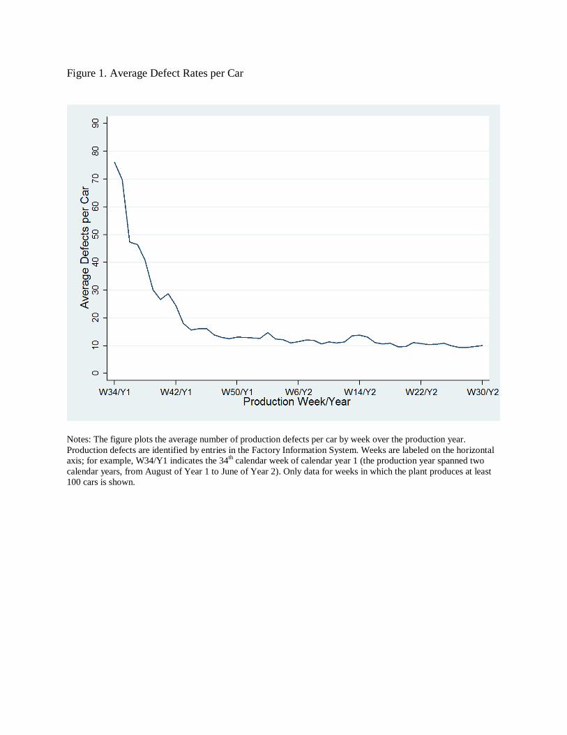
Figure 1. Average Defect Rates per Car

Notes: The figure plots the average number of production defects per car by week over the production year. Production defects are identified by entries in the Factory Information System. Weeks are labeled on the horizontal axis; for example, W34/Y1 indicates the 34th calendar week of calendar year 1 (the production year spanned two calendar years, from August of Year 1 to June of Year 2). Only data for weeks in which the plant produces at least 100 cars is shown.

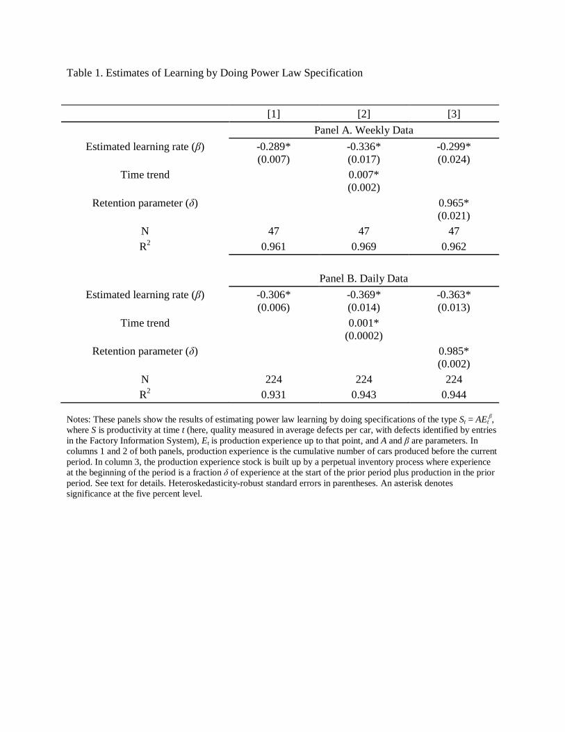
Table 1. Estimates of Learning by Doing Power Law Specification

[1] [2] [3] Panel A. Weekly Data

Estimated learning rate (β) -0.289* (0.007)

-0.336* (0.017)

-0.299* (0.024)

Time trend

0.007* (0.002)

Retention parameter (δ)

0.965* (0.021)

N 47 47 47 R2 0.961 0.969 0.962 Panel B. Daily Data

Estimated learning rate (β) -0.306* (0.006)

-0.369* (0.014)

-0.363* (0.013)

Time trend

0.001* (0.0002)

Retention parameter (δ)

0.985* (0.002)

N 224 224 224 R2 0.931 0.943 0.944

Notes: These panels show the results of estimating power law learning by doing specifications of the type St = AEt

β, where S is productivity at time t (here, quality measured in average defects per car, with defects identified by entries in the Factory Information System), Et is production experience up to that point, and A and β are parameters. In columns 1 and 2 of both panels, production experience is the cumulative number of cars produced before the current period. In column 3, the production experience stock is built up by a perpetual inventory process where experience at the beginning of the period is a fraction δ of experience at the start of the prior period plus production in the prior period. See text for details. Heteroskedasticity-robust standard errors in parentheses. An asterisk denotes significance at the five percent level.

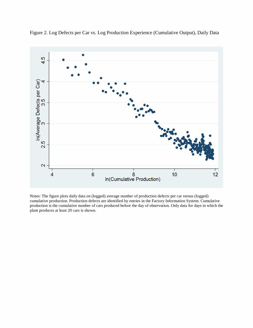
Figure 2. Log Defects per Car vs. Log Production Experience (Cumulative Output), Daily Data

Notes: The figure plots daily data on (logged) average number of production defects per car versus (logged) cumulative production. Production defects are identified by entries in the Factory Information System. Cumulative production is the cumulative number of cars produced before the day of observation. Only data for days in which the plant produces at least 20 cars is shown.

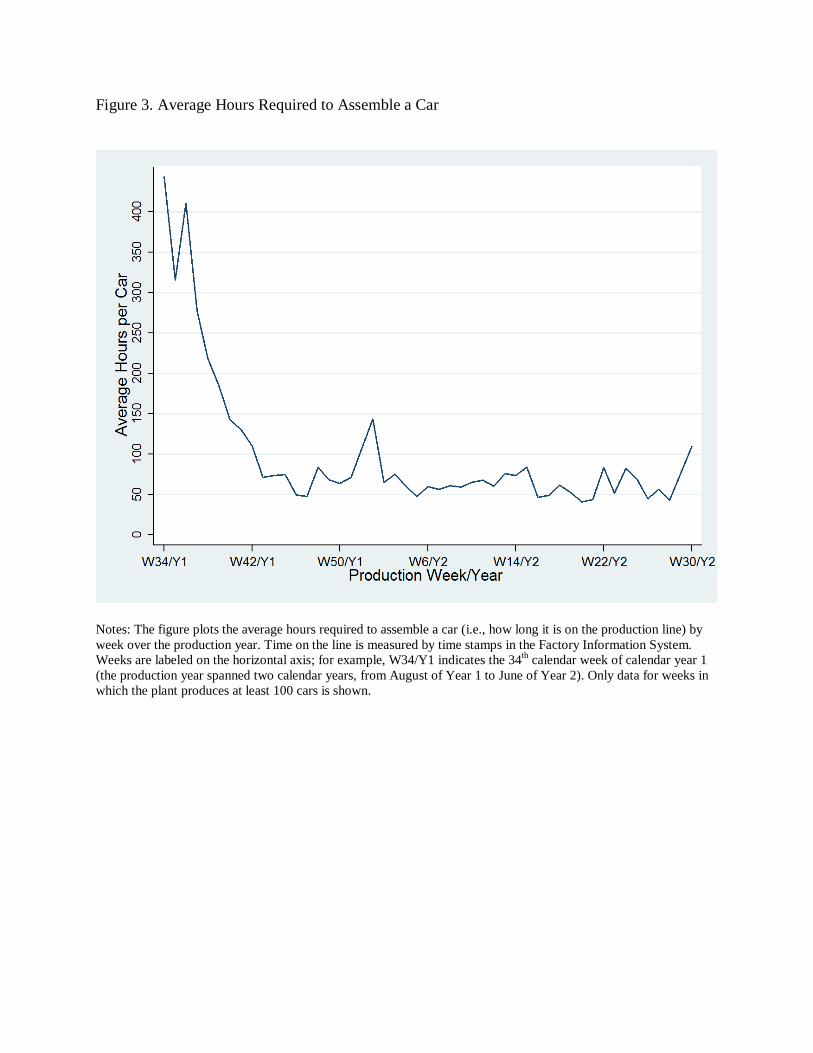
Figure 3. Average Hours Required to Assemble a Car

Notes: The figure plots the average hours required to assemble a car (i.e., how long it is on the production line) by week over the production year. Time on the line is measured by time stamps in the Factory Information System. Weeks are labeled on the horizontal axis; for example, W34/Y1 indicates the 34th calendar week of calendar year 1 (the production year spanned two calendar years, from August of Year 1 to June of Year 2). Only data for weeks in which the plant produces at least 100 cars is shown.

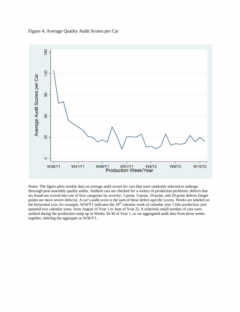
Figure 4. Average Quality Audit Scores per Car

Notes: The figure plots weekly data on average audit scores for cars that were randomly selected to undergo thorough post-assembly quality audits. Audited cars are checked for a variety of production problems; defects that are found are scored into one of four categories by severity: 1-point, 5-point, 10-point, and 20-point defects (larger points are more severe defects). A car’s audit score is the sum of these defect-specific scores. Weeks are labeled on the horizontal axis; for example, W34/Y1 indicates the 34th calendar week of calendar year 1 (the production year spanned two calendar years, from August of Year 1 to June of Year 2). A relatively small number of cars were audited during the production ramp-up in Weeks 34-36 of Year 1, so we aggregated audit data from those weeks together, labeling the aggregate as W36/Y1.

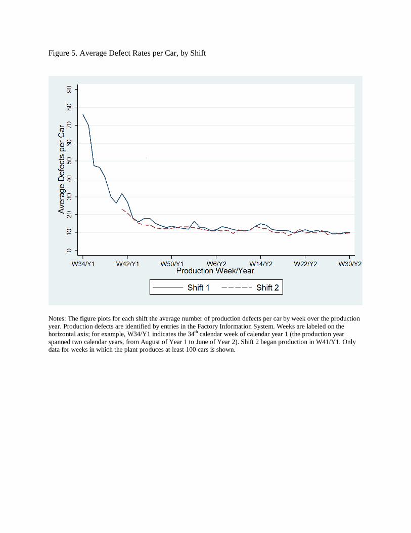
Figure 5. Average Defect Rates per Car, by Shift

Notes: The figure plots for each shift the average number of production defects per car by week over the production year. Production defects are identified by entries in the Factory Information System. Weeks are labeled on the horizontal axis; for example, W34/Y1 indicates the 34th calendar week of calendar year 1 (the production year spanned two calendar years, from August of Year 1 to June of Year 2). Shift 2 began production in W41/Y1. Only data for weeks in which the plant produces at least 100 cars is shown.

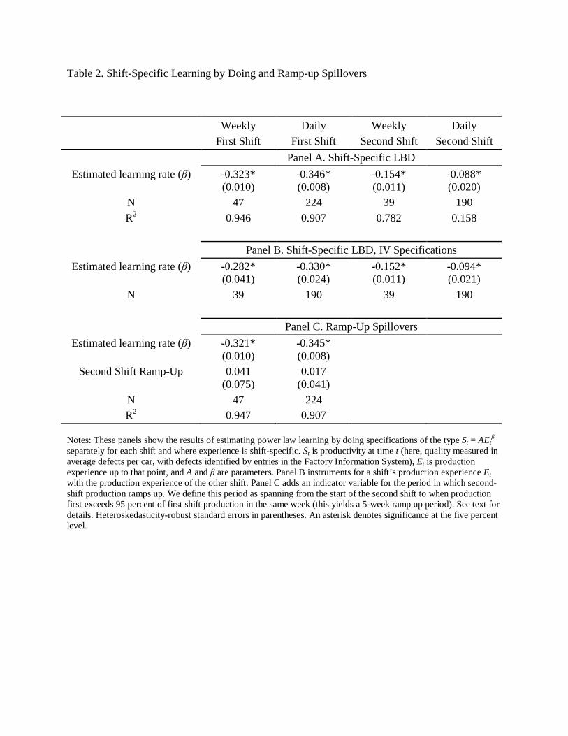
Table 2. Shift-Specific Learning by Doing and Ramp-up Spillovers

Weekly Daily Weekly Daily First Shift First Shift Second Shift Second Shift Panel A. Shift-Specific LBD

Estimated learning rate (β) -0.323* (0.010)

-0.346* (0.008)

-0.154* (0.011)

-0.088* (0.020)

N 47 224 39 190 R2 0.946 0.907 0.782 0.158 Panel B. Shift-Specific LBD, IV Specifications

Estimated learning rate (β) -0.282* (0.041)

-0.330* (0.024)

-0.152* (0.011)

-0.094* (0.021)

N 39 190 39 190 Panel C. Ramp-Up Spillovers

Estimated learning rate (β) -0.321* (0.010)

-0.345* (0.008)

Second Shift Ramp-Up 0.041 (0.075)

0.017 (0.041)

N 47 224 R2 0.947 0.907

Notes: These panels show the results of estimating power law learning by doing specifications of the type St = AEt

β separately for each shift and where experience is shift-specific. St is productivity at time t (here, quality measured in average defects per car, with defects identified by entries in the Factory Information System), Et is production experience up to that point, and A and β are parameters. Panel B instruments for a shift’s production experience Et with the production experience of the other shift. Panel C adds an indicator variable for the period in which second-shift production ramps up. We define this period as spanning from the start of the second shift to when production first exceeds 95 percent of first shift production in the same week (this yields a 5-week ramp up period). See text for details. Heteroskedasticity-robust standard errors in parentheses. An asterisk denotes significance at the five percent level.

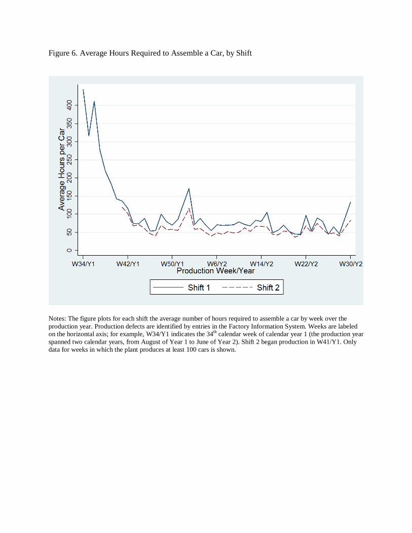
Figure 6. Average Hours Required to Assemble a Car, by Shift

Notes: The figure plots for each shift the average number of hours required to assemble a car by week over the production year. Production defects are identified by entries in the Factory Information System. Weeks are labeled on the horizontal axis; for example, W34/Y1 indicates the 34th calendar week of calendar year 1 (the production year spanned two calendar years, from August of Year 1 to June of Year 2). Shift 2 began production in W41/Y1. Only data for weeks in which the plant produces at least 100 cars is shown.

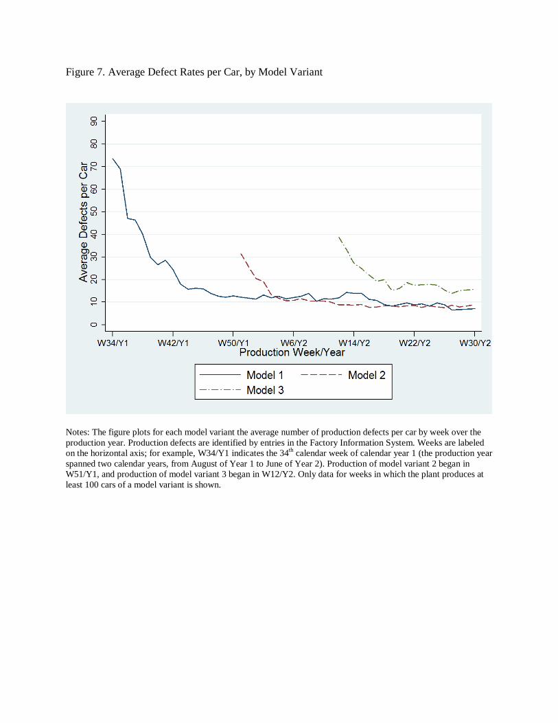
Figure 7. Average Defect Rates per Car, by Model Variant

Notes: The figure plots for each model variant the average number of production defects per car by week over the production year. Production defects are identified by entries in the Factory Information System. Weeks are labeled on the horizontal axis; for example, W34/Y1 indicates the 34th calendar week of calendar year 1 (the production year spanned two calendar years, from August of Year 1 to June of Year 2). Production of model variant 2 began in W51/Y1, and production of model variant 3 began in W12/Y2. Only data for weeks in which the plant produces at least 100 cars of a model variant is shown.

Table 3. Model-Specific Learning by Doing and Ramp-up Spillovers

Weekly Daily Weekly Daily Weekly Daily Model 1 Model 1 Model 2 Model 2 Model 3 Model 3 A. Model-Specific LBD

Estimated learning rate (β) -0.333* (0.014)

-0.356* (0.009)

-0.189* (0.014)

-0.203* (0.014)

-0.219* (0.010)

-0.241* (0.012)

N 47 224 30 142 18 86 R2 0.926 0.880 0.939 0.779 0.923 0.801 B. Ramp-Up Spillovers

Estimated learning rate (β) -0.342* (0.015)

-0.365* (0.010)

-0.188* (0.014)

-0.202* (0.014)

Model 2 Ramp-Up 0.068 (0.042)

0.071* (0.029)

Model 3 Ramp-Up 0.289* (0.060)

0.285* (0.046)

-0.032 (0.018)

-0.040 (0.024)

N 47 224 30 142 R2 0.941 0.894 0.940 0.780

Notes: These panels show the results of estimating power law learning by doing specifications of the type St = AEt

β separately for each model variant and where experience is model-specific. St is productivity at time t (here, quality measured in average defects per car, with defects identified by entries in the Factory Information System), Et is production experience up to that point, and A and β are parameters. Panel B adds indicator variables for periods in which production of later variants ramps up. We define ramp-up periods as beginning when production of the model variant reaches 100 cars per week and ending when production first exceeds 95 percent of the production level of at least one of the models whose production began earlier. This was a five-week period for Model 2 and a three-week period for Model 3. There are no regressions for Model 3, as no new variant is introduced after it. See text for details. Heteroskedasticity-robust standard errors in parentheses. An asterisk denotes significance at the five percent level.

Table 4. Across-Shift, Within-Week Station Defect Quintile Correlations

Station’s Second Shift Quintile in Week 1st 2nd 3rd 4th 5th

Station’s First Shift Quintile in

Week

1st 15.2 5.4 2.8 1.3 0.5 2nd 7.2 3.1 2.5 1.4 0.5 3rd 5.0 4.3 5.7 4.7 1.6 4th 1.5 2.0 4.0 7.2 4.3 5th 0.5 0.5 1.4 4.6 12.7

Notes: This table shows the percentage of production line stations in each quintile of the shift-week’s defect rate distribution. Defects and their station location are identified by entries in the Factory Information System. For example, 15.2 percent of stations in the first quintile of the first shift’s defect rate distribution during the week (i.e., those with the lowest defect rates) were also in the first quintile of the same week’s distribution for the second shift. Another 5.4 percent were in the first quintile of the first shift but the second quintile of the second shift that week, and so on. (Row and column sums aren’t always exactly 20 percent because of ties.)

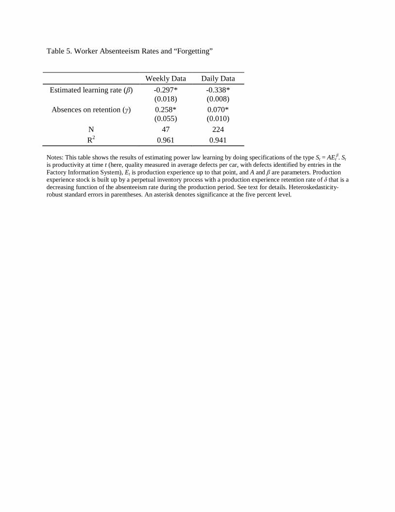
Table 5. Worker Absenteeism Rates and “Forgetting”

Weekly Data Daily Data

Estimated learning rate (β) -0.297* (0.018)

-0.338* (0.008)

Absences on retention (γ) 0.258* (0.055)

0.070* (0.010)

N 47 224 R2 0.961 0.941

Notes: This table shows the results of estimating power law learning by doing specifications of the type St = AEt

β. St is productivity at time t (here, quality measured in average defects per car, with defects identified by entries in the Factory Information System), Et is production experience up to that point, and A and β are parameters. Production experience stock is built up by a perpetual inventory process with a production experience retention rate of δ that is a decreasing function of the absenteeism rate during the production period. See text for details. Heteroskedasticity-robust standard errors in parentheses. An asterisk denotes significance at the five percent level.

Online Appendix

Digging Deeper into the Learning by Doing Mechanism

We explored in the main text the nature of knowledge acquisition, transmission, and

embodiment in the plant. In this additional section, we further leverage our data to deepen our

understanding of the particular mechanisms through which learning takes place.

A. Distribution of Defects across Stations

As discussed above, we see outcomes for each of the several hundred processes that go

into assembling a car. We use these data to answer questions about the composition of process-

specific productivity gains that underlie the more aggregated productivity improvements

analyzed above.

We first explore the process-level distribution of defect rates. Figure A6 shows the

evolution over the sample of various quantiles of the process-specific defect rates. Each

process’s defect rate is computed as the number of defects recorded at that process (station on the

line) in a given workweek divided by the total number of cars produced that week. The figure

sorts these processes into quantiles based on that week’s performance; i.e., a station will move

from one quantile to another over time if its relative defect rate fluctuates.

Panel A of Figure A6 shows the 50th, 75th, and 95th percentiles of the absolute levels of

station-level defect rates (the skewness of the distribution relative to the scale of the figure

makes it very difficult to visually distinguish quantiles below the median). Defect rates are

highly skewed across stations, with a thick right tail. In the first full week of production, for

example, the defect rate at the 95th percentile station is 20 times the rate at the median station that

week, and five times the 75th percentile rate. The tightening of the distribution early in the

production year indicates that the large early-period productivity gains seen in the aggregate

series come largely from defect reductions in the right tail of stations. Interestingly, though, the

basic shape of the distribution stays the same throughout the production year. This can be seen in

panel B of Figure A6, which shows the ratio of a quantile’s defect rate in a particular week to

that same quantile’s defect rate during the first week of production. We add the 25th percentile

series to this panel, as it can now be distinguished from the others. That is, the panel shows the

percentage decline of the quantile’s defect rate relative to itself. All quantiles follow essentially

the same pattern, with considerable reductions in relative defect rates early in the production

period that decelerate over time. Aggregate learning by doing at the plant therefore reflects a

proportional tightening of the entire station-level defect rate distribution, with all quantiles

experiencing similar percentage declines in defect rates.25

It does not appear, therefore, that

productivity gains reflect all-out efforts to address the most problematic assembly procedures

while ignoring all the others. The relative defect rates of all processes fall essentially in tandem.

B. Persistence of Station-Level Defects

Figure A6 sheds no light on the question of whether the persistence of defect rates for a

given processes. Specific processes could be relatively defect prone (or defect free) throughout

the year, or they could jump from quantile to quantile, being major sources of defects at one

point during the year while being nearly defect free at other times. To investigate persistence, we

first split the model year production into three equal-length periods: beginning, middle, and end.

We then calculate the station-level defect rate distribution within the first period, and assign a

station to its quintile in the distribution during that period. We then count defects in each of the

three periods by the first-period quintile of their process. The fewer changes we observe in the

relative contribution of a particular quintile over time, the more persistence there is in process-

level defect rates.

We present the results of this exercise in Figure A7, which can be interpreted as follows.

Panel A shows the results for the total number of production defects during the period. The bar

labeled “1” breaks the total number of defects that occurred during the first production period,

about one million, into quintile-specific components. The top portion of the bar is the portion of

defects that occurred in the stations in the top quintile of the distribution. The skewness of the

defect distribution analyzed previously is obvious in this figure as well; roughly 90 percent of all

defects occurred at stations in the top quintile. Further, almost all of the remaining 10 percent of

defects occurred at stations in the second quintile of the defect distribution, as indicated by the

second color in the bar. Stations in the bottom three quintiles account for a miniscule portion of

the total number of defects during the period.

The bar labeled “2” repeats the exercise for the second production period, but it holds the

quintile assignments constant. Note first that the height of the overall bar is lower in period two

25 The quantiles of the distribution are computed while including stations that report no defects, which number between 7-14 percent of stations in any given week. Qualitatively similar data patterns remain in both absolute and relative defect levels among the corresponding quantiles of the distribution conditional on stations reporting at least one production defect during the week.

because there are fewer total defects in this period is lower because of learning by doing.

Because quintile assignments are held constant across time in Figure A7, the top color in the bar

shows the number of defects in the second production period that are accounted for by stations

that were in the top quintile of the distribution in the first period. If defect rates within stations

have no persistence and are completely random over time, then we should expect each first-

period quintile will account for 20 percent of all errors in the later two periods. This is clearly not

the case. Stations at the right tail of the distribution in the first period still account for the vast

majority of production defects in the second period.

The bottom three quintiles again account for only a tiny part of the total number of

defects in the period. Defect rates at the station level are therefore quite persistent. There is some

shift in stations’ locations in the defect rate distribution, however, as the share of defects

accounted for by top-quintile stations does shrink between the first and second periods. This can

be seen more easily in the proportional results in panel B of Figure A7, shows values in terms of

the share of defects in the period rather than the absolute number. These same patterns hold in

the period 3 results. While total defect rates fall, the most error-prone stations early on the model

year still account for a large fraction of the defects at the end of the year, again indicating a large

degree of persistence in a process’s propensity to lead to production defects.

C. Defect Spillovers across Cars

Our final investigation explores whether defect rates are correlated across cars produced

in sequence. That is, we examine to what extent the probability of defects occurring spills over

across adjacent cars on the production line. There are several mechanisms through which this

could happen. If a defect occurs on one particular car, a worker may sometimes attempt to rectify

the problem before the car moves to the next production process. This can lead to a longer time

being spent on the operation than typical, reducing the time available for the operation on the

following vehicle, which could in turn result in another defect on that car. Further, when a defect

is not addressed at the location it occurs, a worker further down the line might sometimes

attempt a fix. This could in turn result in a defect occurring in an adjacent car at that later station.

More broadly, if a worker is distracted or otherwise performing poorly, then s/he is likely to be

distracted on consecutive cars.

We are interested in spillovers in our context because one way learning-based

productivity improvements can occur is if production experience reveals how to limit the extent

of spillovers. To see how this might work, imagine a stylized world where a certain number of

defects happen by random chance, and the nature of these defects is to adversely impact every

car until someone catches and fixes the mistake. Learning-based productivity gains in this world

could come from two sources: a reduction in the probability that defects arise in the first place, or

more expedient identification and rectification of the defects that arise.

We investigate the issue by estimating a model that relates defects on one car to those on

adjacent cars on the line. Specifically, we regress the defect count of a given car on the defect

counts for each of the 40 cars that preceded it along the line:

(4) 𝑆𝑐𝑡 = ∑ 𝛼𝑘𝑆𝑐+𝑘,𝑡40𝑘=1 + 𝜃𝑡 + 𝜀𝑐𝑡,

where Sct is the defect count for car c produced on day t, Sc+1,t through Sc+40,t are the defect counts

for the 40 cars preceding car c on the production line, θt is a day fixed effect, and εct is an error

term. The coefficients αk give the marginal effect of a defect on car c + k on the defect count of

car c (this is analogous to an autoregressive model where a variable is regressed on its preceding

values, and the coefficients reflect the marginal effect of a change in the value in k periods prior

on the value in period c). Day fixed effects control for changes in average defect rates over the

sample period. Thus the coefficients in this model reflect whether, relative to other cars produced

on that day, defects on proximate cars lead the reference car to have more problems. If spillovers

exist, higher defects on one car will lead to more defects on those that follow it in the production

sequence. We estimate this specific separately for three different production periods: early in the

model year, in the middle of the year, and toward year’s end, to see if any spillover patterns

change over the production year.

We show empirical results in Figure A8. Panels A through C show the estimated

regression coefficients for each of the three production periods (early, middle, and final thirds of

the year, defined as in our persistence analysis above), along with their 95-percent confidence

intervals. We only plot the coefficients for the 25 cars prior to the reference car, as this is

sufficient to see where spillover effects become statistically insignificant. Spillovers clearly

exist. Production defects on one car raise the likelihood of defects on cars that come later in line.

As one might expect, the magnitude of these spillovers falls as the distance between cars on the

assembly line grows. Still, defects on one car have statistically significant spillovers on at least

the next 15 cars on the line. In terms of magnitudes, a one-defect “shock” on a given car leads,

on average, to about one-ninth of a defect on the next car in the line (or equivalently, an extra

defect on the following car one-ninth of the time). The same shock leads to roughly 0.08 defects

on the car that comes two positions later. The tenth car down the line experiences 0.02 more

defects on average.

It does not appear, however, that a decrease in spillover effects during the production

year explains the plant’s learning by doing patterns. This can be seen in panel D of Figure A8,

which overlays the coefficient estimates for the three time periods on a common set of axes. The

three sets of coefficients have basically the same shape, with no noticeable decline in the size of

defect spillovers across the production year.

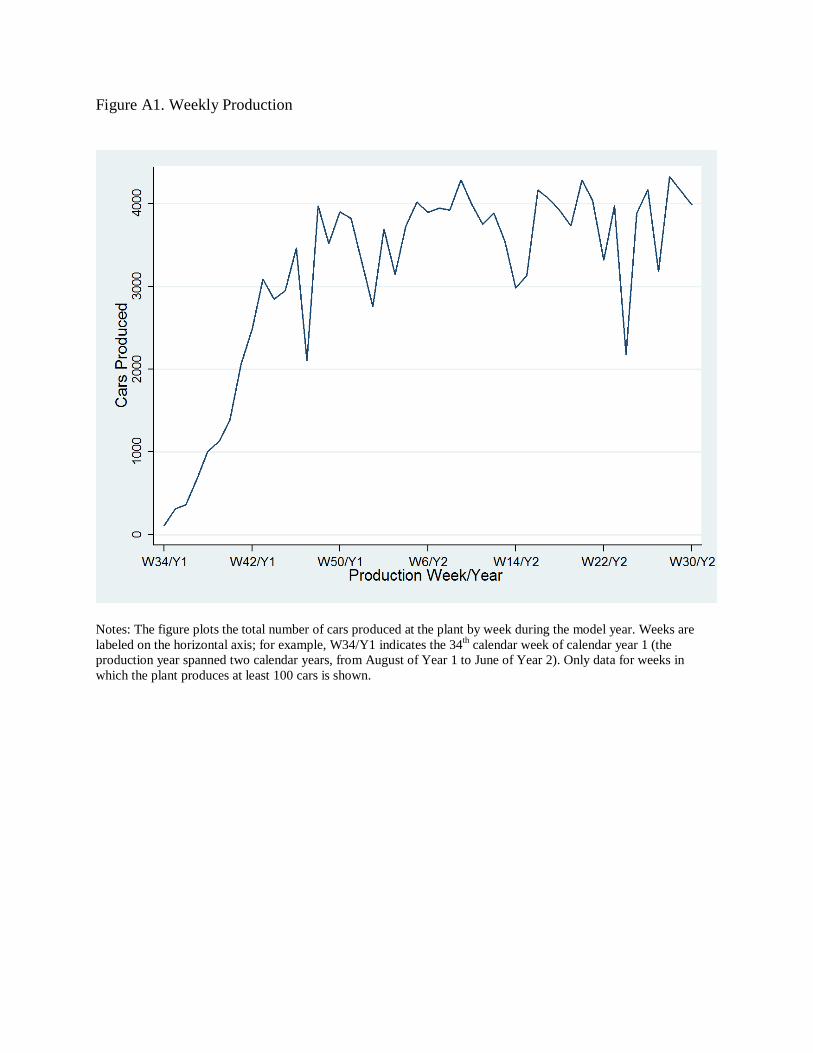
Figure A1. Weekly Production

Notes: The figure plots the total number of cars produced at the plant by week during the model year. Weeks are labeled on the horizontal axis; for example, W34/Y1 indicates the 34th calendar week of calendar year 1 (the production year spanned two calendar years, from August of Year 1 to June of Year 2). Only data for weeks in which the plant produces at least 100 cars is shown.

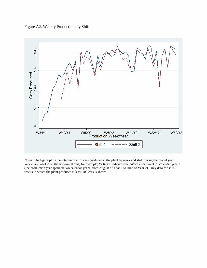
Figure A2. Weekly Production, by Shift

Notes: The figure plots the total number of cars produced at the plant by week and shift during the model year. Weeks are labeled on the horizontal axis; for example, W34/Y1 indicates the 34th calendar week of calendar year 1 (the production year spanned two calendar years, from August of Year 1 to June of Year 2). Only data for shift-weeks in which the plant produces at least 100 cars is shown.

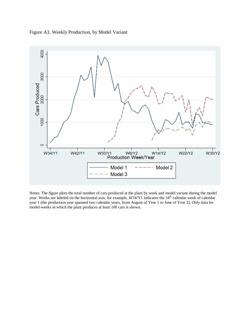
Figure A3. Weekly Production, by Model Variant

Notes: The figure plots the total number of cars produced at the plant by week and model variant during the model year. Weeks are labeled on the horizontal axis; for example, W34/Y1 indicates the 34th calendar week of calendar year 1 (the production year spanned two calendar years, from August of Year 1 to June of Year 2). Only data for model-weeks in which the plant produces at least 100 cars is shown.

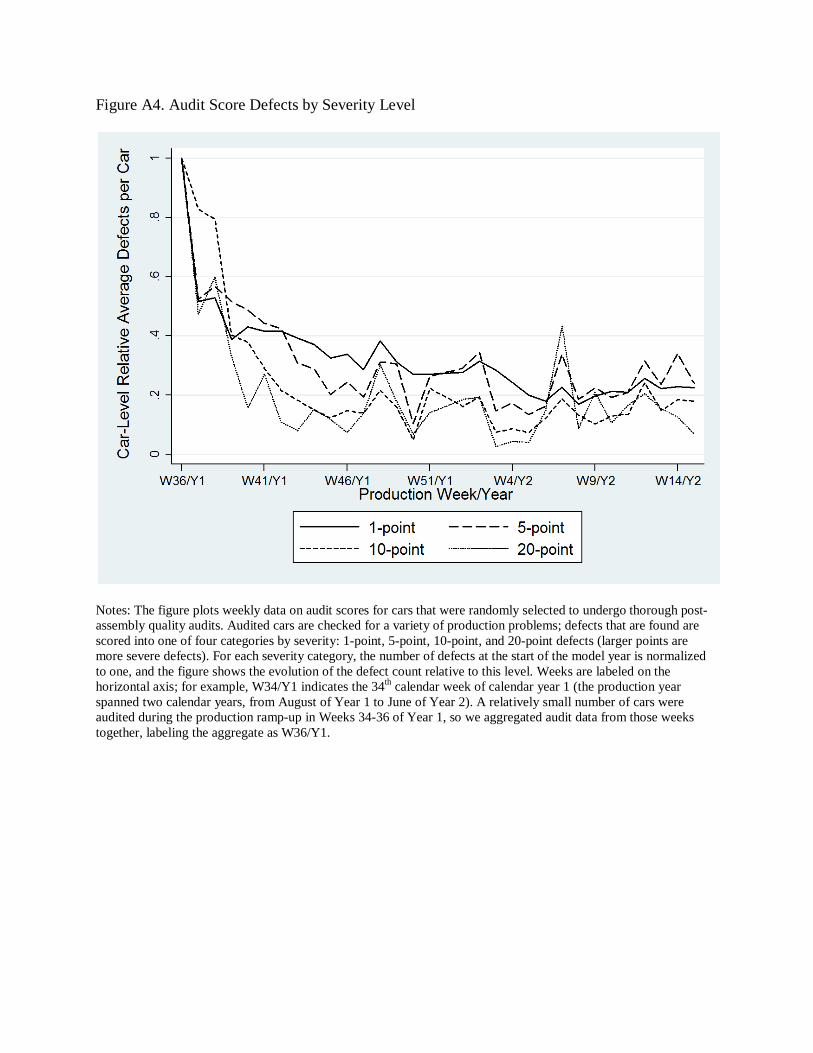
Figure A4. Audit Score Defects by Severity Level

Notes: The figure plots weekly data on audit scores for cars that were randomly selected to undergo thorough post-assembly quality audits. Audited cars are checked for a variety of production problems; defects that are found are scored into one of four categories by severity: 1-point, 5-point, 10-point, and 20-point defects (larger points are more severe defects). For each severity category, the number of defects at the start of the model year is normalized to one, and the figure shows the evolution of the defect count relative to this level. Weeks are labeled on the horizontal axis; for example, W34/Y1 indicates the 34th calendar week of calendar year 1 (the production year spanned two calendar years, from August of Year 1 to June of Year 2). A relatively small number of cars were audited during the production ramp-up in Weeks 34-36 of Year 1, so we aggregated audit data from those weeks together, labeling the aggregate as W36/Y1.

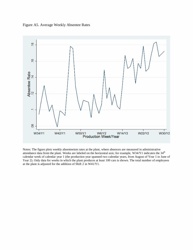
Figure A5. Average Weekly Absentee Rates

Notes: The figure plots weekly absenteeism rates at the plant, where absences are measured in administrative attendance data from the plant. Weeks are labeled on the horizontal axis; for example, W34/Y1 indicates the 34th calendar week of calendar year 1 (the production year spanned two calendar years, from August of Year 1 to June of Year 2). Only data for weeks in which the plant produces at least 100 cars is shown. The total number of employees at the plant is adjusted for the addition of Shift 2 in W41/Y1.

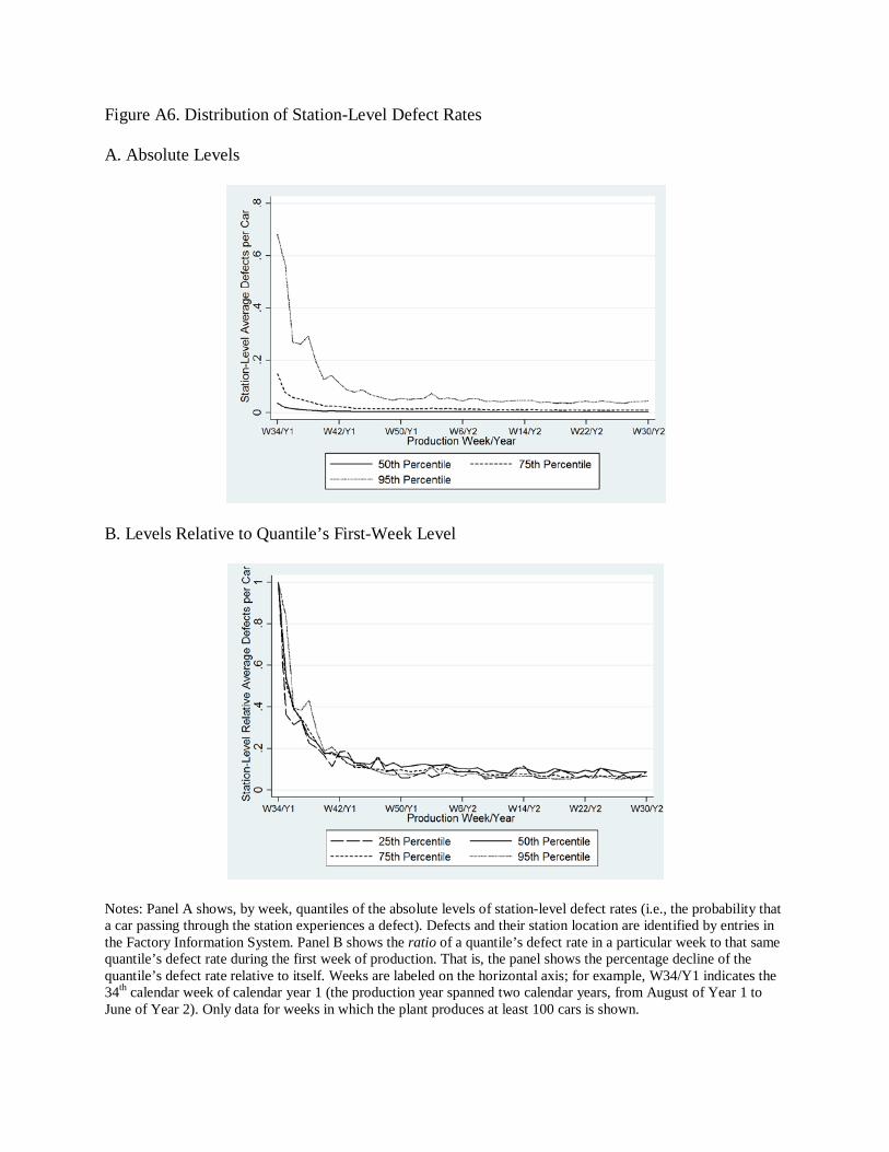
Figure A6. Distribution of Station-Level Defect Rates A. Absolute Levels

B. Levels Relative to Quantile’s First-Week Level

Notes: Panel A shows, by week, quantiles of the absolute levels of station-level defect rates (i.e., the probability that a car passing through the station experiences a defect). Defects and their station location are identified by entries in the Factory Information System. Panel B shows the ratio of a quantile’s defect rate in a particular week to that same quantile’s defect rate during the first week of production. That is, the panel shows the percentage decline of the quantile’s defect rate relative to itself. Weeks are labeled on the horizontal axis; for example, W34/Y1 indicates the 34th calendar week of calendar year 1 (the production year spanned two calendar years, from August of Year 1 to June of Year 2). Only data for weeks in which the plant produces at least 100 cars is shown.

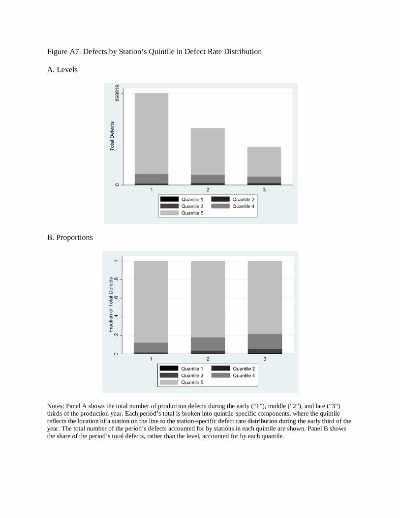
Figure A7. Defects by Station’s Quintile in Defect Rate Distribution A. Levels

B. Proportions

Notes: Panel A shows the total number of production defects during the early (“1”), middle (“2”), and late (“3”) thirds of the production year. Each period’s total is broken into quintile-specific components, where the quintile reflects the location of a station on the line to the station-specific defect rate distribution during the early third of the year. The total number of the period’s defects accounted for by stations in each quintile are shown. Panel B shows the share of the period’s total defects, rather than the level, accounted for by each quantile.

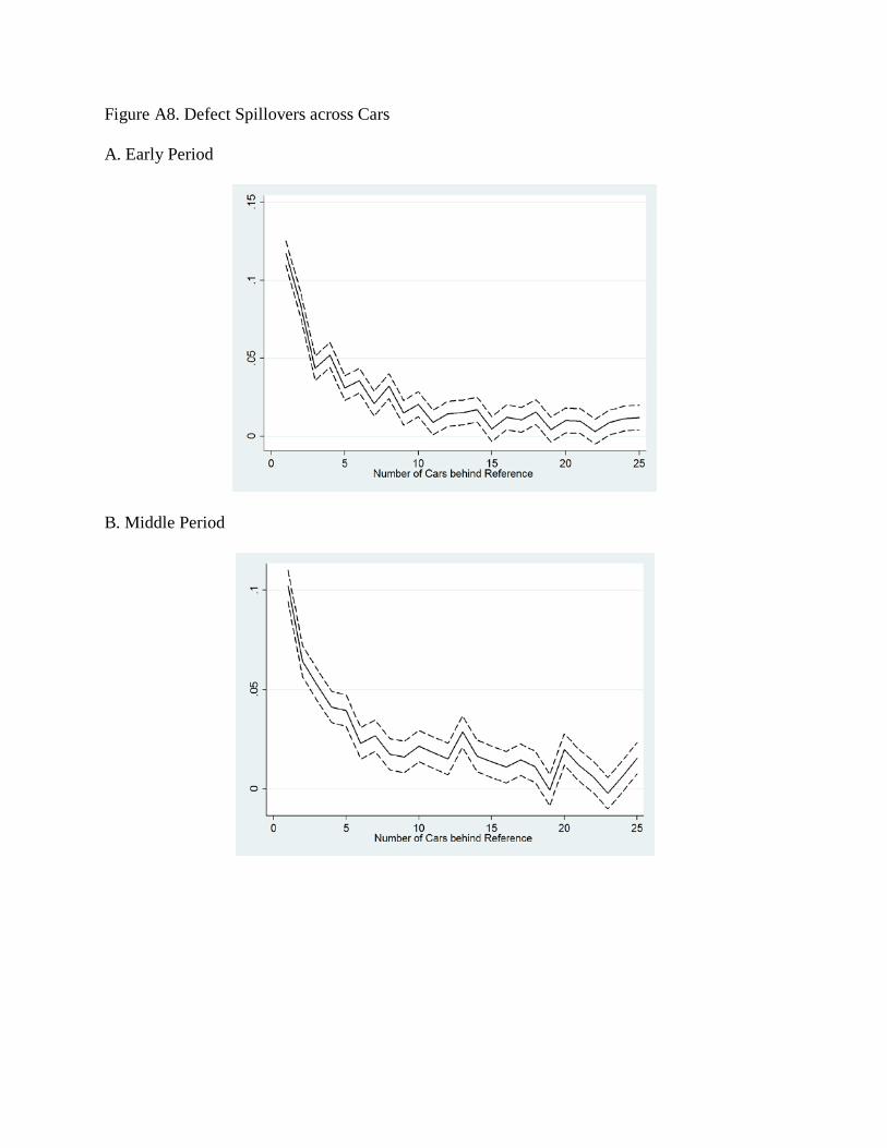
Figure A8. Defect Spillovers across Cars A. Early Period

B. Middle Period

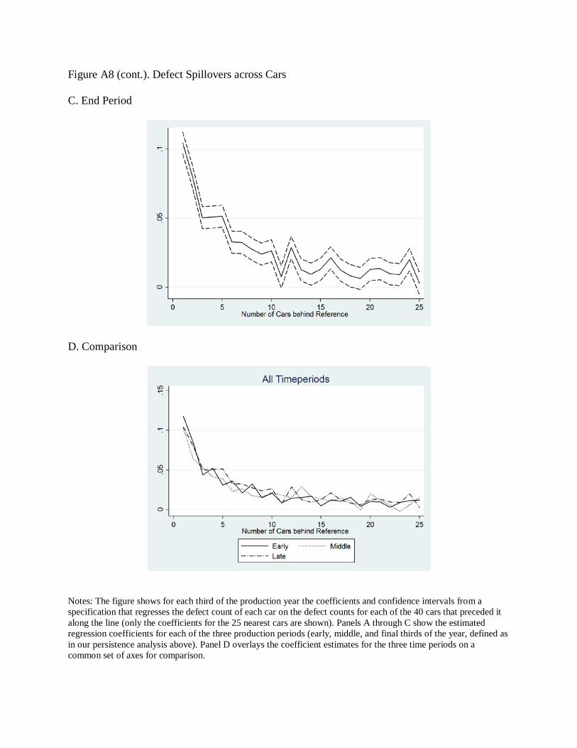
Figure A8 (cont.). Defect Spillovers across Cars C. End Period

D. Comparison

Notes: The figure shows for each third of the production year the coefficients and confidence intervals from a specification that regresses the defect count of each car on the defect counts for each of the 40 cars that preceded it along the line (only the coefficients for the 25 nearest cars are shown). Panels A through C show the estimated regression coefficients for each of the three production periods (early, middle, and final thirds of the year, defined as in our persistence analysis above). Panel D overlays the coefficient estimates for the three time periods on a common set of axes for comparison.