TOTAL VARIATION CUTOFF IN BIRTH-AND-DEATH …eyal/papers/birthdeath.pdfducible birth-and-death chains, as well as for -lazy discrete chains (where P(x;x) for all x 2). In what follows,

TOTAL VARIATION CUTOFF IN BIRTH-AND-DEATH CHAINS

JIAN DING, EYAL LUBETZKY AND YUVAL PERES

A. The cutoff phenomenon describes a case where a Markovchain exhibits a sharp transition in its convergence to stationarity. In1996, Diaconis surveyed this phenomenon, and asked how one couldrecognize its occurrence in families of finite ergodic Markov chains. In2004, the third author noted that a necessary condition for cutoff in afamily of reversible chains is that the product of the mixing-time andspectral-gap tends to infinity, and conjectured that in many settings, thiscondition should also be sufficient. Diaconis and Saloff-Coste (2006)verified this conjecture for continuous-time birth-and-death chains, sta-rted at an endpoint, with convergence measured in separation. It is nat-ural to ask whether the conjecture holds for these chains in the morewidely used total-variation distance.

In this work, we confirm the above conjecture for all continuous-timeor lazy discrete-time birth-and-death chains, with convergence measuredvia total-variation distance. Namely, if the product of the mixing-timeand spectral-gap tends to infinity, the chains exhibit cutoff at the maximalhitting time of the stationary distribution median, with a window of atmost the geometric mean between the relaxation-time and mixing-time.

In addition, we show that for any lazy (or continuous-time) birth-and-death chain with stationary distribution π, the separation 1− pt(x, y)/π(y)is maximized when x, y are the endpoints. Together with the above re-sults, this implies that total-variation cutoff is equivalent to separationcutoff in any family of such chains.

1. I

The cutoff phenomenon arises when a finite Markov chain convergesabruptly to equilibrium. Roughly, this is the case where, over a negligi-ble period of time known as the cutoff window, the distance of the chainfrom the stationary measure drops from near its maximum to near 0.

Let (Xt) denote an aperiodic irreducible Markov chain on a finite statespace Ω with transition kernel P(x, y), and let π denote its stationary distri-bution. For any two distributions µ, ν on Ω, their total-variation distance is

Research of J. Ding and Y. Peres was supported in part by NSF grant DMS-0605166.1

2 JIAN DING, EYAL LUBETZKY AND YUVAL PERES

defined to be

‖µ − ν‖TV := supA⊂Ω

|µ(A) − ν(A)| =12

∑x∈Ω

|µ(x) − ν(x)| .

Consider the worst-case total-variation distance to stationarity at time t,

d(t) := maxx∈Ω‖Px(Xt ∈ ·) − π‖TV ,

where Px denotes the probability given X0 = x. The total-variation mixing-time of (Xt), denoted by t(ε) for 0 < ε < 1, is defined to be

t(ε) := min t : d(t) ≤ ε .

Next, consider a family of such chains, (X(n)t ), each with its corresponding

worst-distance from stationarity dn(t), its mixing-times t(n), etc. We say that

this family of chains exhibits cutoff iff the following sharp transition in itsconvergence to stationarity occurs:

limn→∞

t(n)(ε)

t(n)(1 − ε)

= 1 for any 0 < ε < 1 . (1.1)

Our main result is an essentially tight bound on the difference betweent(ε) and t(1 − ε) for general birth-and-death chains; a birth-and-deathchain has the state space 0, . . . , n for some integer n, and always movesfrom one state to a state adjacent to it (or stays in place).

We first state a quantitative bound for a single chain, then deduce a cutoff

criterion. Let gap be the spectral-gap of the chain (that is, gap := 1 − λwhere λ is the largest absolute-value of all nontrivial eigenvalues of thetransition kernel P), and let t := gap−1 denote the relaxation-time of thechain. A chain is called lazy if P(x, x) ≥ 1

2 for all x ∈ Ω.

Theorem 1. For any 0 < ε < 12 there exists an explicit cε > 0 such that

every lazy irreducible birth-and-death chain (Xt) satisfies

t(ε) − t(1 − ε) ≤ cε√

t · t( 14 ) . (1.2)

As we later show, the above theorem extends to continuous-time chains,as well as to δ-lazy chains, which satisfy P(x, x) ≥ δ for all x ∈ Ω.

The notion of a cutoff-window relates Theorem 1 to the cutoff phenome-non. A sequence wn is called a cutoff window for a family of chains (X(n)

t )if the following holds: wn = o

(t(n)( 1

4 )), and for any ε > 0 there exists some

cε > 0 such that, for all n,

t(n)(ε) − t(n)

(1 − ε) ≤ cεwn . (1.3)

TOTAL VARIATION CUTOFF IN BIRTH-AND-DEATH CHAINS 3

Equivalently, if tn and wn are two sequences such that wn = o(tn), one maydefine that a sequence of chains exhibits cutoff at tn with window wn iff

limλ→∞ lim infn→∞ dn(tn − λwn) = 1 ,limλ→∞ lim supn→∞ dn(tn + λwn) = 0 .

To go from the first definition to the second, take tn = t(n)( 1

4 ).Once we compare the forms of (1.2) and (1.3), it becomes clear that

Theorem 1 implies a bound on the cutoff window for any general family ofbirth-and-death chains, provided that t(n)

= o(t(n)(1

4 )).

Theorem 1 will be the key to establishing the criterion for total-variationcutoff in a general family of birth-and-death chains.

1.1. Background. The cutoff phenomenon was first identified for the caseof random transpositions on the symmetric group in [11], and for the caseof random walks on the hypercube in [1]. It was given its name by Aldousand Diaconis in their famous paper [3] from 1985, where they showed thatthe top-in-at-random card shuffling process (repeatedly removing the topcard and reinserting it to the deck at a random position) has such a behavior.Saloff-Coste [25] surveys the cutoff phenomenon for random walks on finitegroups.

Though many families of chains are believed to exhibit cutoff, provingthe occurrence of this phenomenon is often an extremely challenging task,hence there are relatively few examples for which cutoff has been rigorouslyshown. In 1996, Diaconis [7] surveyed the cutoff phenomenon, and asked ifone could determine whether or not it occurs in a given family of aperiodicand irreducible finite Markov chains.

In 2004, the third author [24] observed that a necessary condition forcutoff in a family of reversible chains is that the product t(n)

(14 ) · gap(n)

tends to infinity with n, or equivalently, t(n) = o

(t(n)( 1

4 )); see Lemma 2.1.

The third author also conjectured that, in many natural classes of chains,

Cutoff occurs if and only if t(n) = o

(t(n)(1

4 ))

. (1.4)

In the general case, this condition does not always imply cutoff : Aldous[2] and Pak (private communication via P. Diaconis) have constructed rel-evant examples (see also [5],[6] and [21]). This left open the question ofcharacterizing the classes of chains for which (1.4) holds.

One important class is the family of birth-and-death chains; see [10] formany natural examples of such chains. They also occur as the magnetiza-tion chain of the mean-field Ising Model (see [12],[20]).

In 2006, Diaconis and Saloff-Coste [10] verified a variant of the conjec-ture (1.4) for birth-and-death chains, when the convergence to stationarity ismeasured in separation, that is, according to the decay of sep(P0(Xt ∈ ·), π),


where sep(µ, ν) = supx∈Ω(1 − µ(x)ν(x) ). Note that, although sep(µ, ν) assumes

values in [0, 1], it is in fact not a metric (it is not even symmetric). See, e.g.,[4, Chapter 4] for the connections between mixing-times in total-variationand in separation.

More precisely, it was shown in [10] that any family of continuous-timebirth-and-death chains, started at 0, exhibits cutoff in separation if and onlyif t(n) = o

(t(n)sep(1

4 ; 0)), where tsep(ε; s) = mint : sep(Ps(Xt ∈ ·), π) < ε. The

proof used a spectral representation of passage times [16,17] and duality ofstrong stationary times. Whether (1.4) holds with respect to the importantand widely used total-variation distance, remained unsettled.

1.2. Total-variation cutoff. In this work, we verify the conjecture (1.4) forarbitrary birth-and-death chains, with the convergence to stationarity mea-sured in total-variation distance. Our first result, which is a direct corollaryof Theorem 1, establishes this for lazy discrete-time irreducible birth-and-death chains. We then derive versions of this result for continuous-time irre-ducible birth-and-death chains, as well as for δ-lazy discrete chains (whereP(x, x) ≥ δ for all x ∈ Ω). In what follows, we omit the dependence on nwherever it is clear from the context.

Corollary 2. Let (X(n)t ) be a sequence of lazy irreducible birth-and-death

chains. Then it exhibits cutoff in total-variation distance iff t(n) · gap(n)

tends to infinity with n. Furthermore, the cutoff window size is at most thegeometric mean between the mixing-time and relaxation time.

As we will later explain, the given bound√

t · t for the cutoff win-dow is essentially tight, in the following sense. Suppose that the functionstM(n) and tR(n) ≥ 2 denote the mixing-time and relaxation-time of (X(n)

t ), afamily of irreducible lazy birth-and-death chains. Then there exists a fam-ily (Y (n)

t ) of such chains with the parameters t(n) = (1 + o(1))tM(n) and

t(n) = (1 + o(1))tR(n) that has a cutoff window of (t(n)

· t(n))1/2. In other

words, no better bound on the cutoff window can be given without exploit-ing additional information on the chains.

Indeed, there are examples where additional attributes of the chain implya cutoff window of order smaller than

√t · t. For instance, the cutoff

window has size t for the Ehrenfest urn (see, e.g., [9]) and for the magne-tization chain in the mean field Ising Model at high temperature (see [12]).

Theorem 3.1, given in Section 3, extends Corollary 2 to the case of δ-lazydiscrete-time chains. We note that this is in fact the setting that correspondsto the magnetization chain in the mean-field Ising Model (see, e.g., [20]).

Following is the continuous-time version of Corollary 2.


Theorem 3. Let (X(n)t ) be a sequence of continuous-time birth-and-death

chains. Then (X(n)t ) exhibits cutoff in total-variation iff t(n)

= o(t(n)), and the

cutoff window size is at most√

t(n)( 1

4 ) · t(n).

By combining our results with those of [10] (while bearing in mind therelation between the mixing-times in total-variation and in separation), onecan relate worst-case total-variation cutoff in any continuous-time familyof irreducible birth-and-death chains, to cutoff in separation started from 0.This suggests that total-variation cutoff should be equivalent to separationcutoff in such chains under the original definition of the worst starting point(as opposed to fixing the starting point at one of the endpoints). Indeed,it turns out that for any lazy or continuous-time birth-and-death chain, theseparation is always attained by the two endpoints, as formulated by thenext proposition.

Proposition 4. Let (Xt) be a lazy (or continuous-time) birth-and-death chainwith stationary distribution π. Then for every integer (resp. real) t > 0, theseparation 1 − Px(Xt = y)/π(y) is maximized when x, y are the endpoints.

That is, for such chains, the maximal separation from π at time t issimply 1 − Pt(0, n)/π(n) (for the lazy chain with transition kernel P) or1 − Ht(0, n)/π(n) (for the continuous-time chain with heat kernel Ht). Aswe later show, this implies the following corollary:

Corollary 5. For any continuous-time family of irreducible birth-and-deathchains, cutoff in worst-case total-variation distance is equivalent to cutoffin worst-case separation.

Note that, clearly, the above equivalence is in the sense that one cutoff

implies the other, yet the cutoff locations need not be equal (and sometimesindeed are not equal, e.g., the Bernoulli-Laplace models, surveyed in [10,Section 7]).

The rest of this paper is organized as follows. The proofs of Theorem 1and Corollary 2 appear in Section 2. Section 3 contains the proofs of thevariants of Theorem 1 for the continuous-case (Theorem 3) and the δ-lazycase. In Section 4, we discuss separation in general birth-and-death chains,and provide the proofs of Proposition 4 and Corollary 5. The final section,Section 5, is devoted to concluding remarks and open problems.

2. C --

In this section we prove the main result, which shows that the conditiongap · t → ∞ is necessary and sufficient for total-variation cutoff in lazybirth-and-death chains.


2.1. Proof of Corollary 2. The fact that any family of lazy irreduciblebirth-and-death chains satisfying t · gap → ∞ exhibits cutoff, followsby definition from Theorem 1, as does the bound

√t · t on the cutoff

window size.It remains to show that this condition is necessary for cutoff; this is known

to hold for any family of reversible Markov chains, using a straightforwardand well known lower bound on t in terms of t (cf., e.g., [21]). Weinclude its proof for the sake of completeness.

Lemma 2.1. Let (Xt) denote a reversible Markov chain, and suppose thatt ≥ 1 + θt(1

4 ) for some fixed θ > 0. Then for any 0 < ε < 1

t(ε) ≥ t( 14 ) · θ log(1/2ε) . (2.1)

In particular, t(ε)/t( 14 ) ≥ K for all K > 0 and ε < 1

2 exp(−K/θ).

Proof. Let P denote the transition kernel of X, and recall that the fact thatX is reversible implies that P is a symmetric operator with respect to 〈·, ·〉πand 1 is an eigenfunction corresponding to the trivial eigenvalue 1.

Let λ denote the largest absolute-value of all nontrivial eigenvalues of P,and let f be the corresponding eigenfunction, P f = ±λ f , normalized tohave ‖ f ‖∞ = 1. Finally, let r be the state attaining | f (r)| = 1. Since f isorthogonal to 1, it follows that for any t,

λt =∣∣∣(Pt f )(r) − 〈 f , 1〉π

∣∣∣ ≤ maxx∈Ω

∣∣∣∣∑y∈Ω

Pt(x, y) f (y) − π(y) f (y)∣∣∣∣

≤ ‖ f ‖∞maxx∈Ω‖Pt(x, ·) − π‖1 = 2 max

x∈Ω‖Pt(x, ·) − π‖TV .

Therefore, for any 0 < ε < 1 we have

t(ε) ≥ log1/λ(1/2ε) ≥log(1/2ε)λ−1 − 1

= (t − 1) log(1/2ε) , (2.2)

and (2.1) immediately follows.

This completes the proof of Corollary 2.

2.2. Proof of Theorem 1. The essence of proving the theorem lies in thetreatment of the regime where t is much smaller than t( 1

4 ).

Theorem 2.2. Let (Xt) denote a lazy irreducible birth-and-death chain, andsuppose that t < ε5 · t(1

4 ) for some 0 < ε < 116 . Then

t(4ε) − t(1 − 2ε) ≤ (6/ε)√

t · t(14 ) .

Proof of Theorem 1. To prove Theorem 1 from Theorem 2.2, let ε > 0,and suppose first that t < ε5 · t( 1

4 ). If ε < 164 , then the above theorem

clearly implies that (1.2) holds for cε = 24/ε. Since that the left-hand-side


of (1.2) is monotone decreasing in ε, this result extends to any value ofε < 1

2 by choosing

c1 = c1(ε) = 24 max1/ε, 64 .

It remains to treat the case where t ≥ ε5 · t(14 ). In this case, the sub-

multiplicativity of the mixing-time (see, e.g., [4, Chapter 2]) gives

t(ε) ≤ t(14 )d 1

2 log2(1/ε)e for any 0 < ε < 14 . (2.3)

In particular, for ε < 14 our assumption on t gives

t(ε) − t(1 − ε) ≤ t(ε) ≤ ε−5/2 log2(1/ε)√

t · t( 14 ) .

Therefore, a choice of

c2 = c2(ε) = maxlog2(1/ε)/ε5/2, 64

gives (1.2) for any ε < 12 (the case ε > 1

4 again follows from monotonicity).Altogether, a choice of cε = maxc1, c2 completes the proof.

In the remainder of this section, we provide the proof of Theorem 2.2. Tothis end, we must first establish several lemmas.

Let X = X(t) be the given (lazy irreducible) birth-and-death chain, andfrom now on, let Ωn = 0, . . . , n denote its state space. Let P denote thetransition kernel of X, and let π denote its stationary distribution. Our firstargument relates the mixing-time of the chain, starting from various startingpositions, with its hitting time from 0 to certain quantile states, defined next.

Q(ε) := mink :

k∑j=0

π( j) ≥ ε, where 0 < ε < 1 . (2.4)

Similarly, one may define the hitting times from n as follows:

Q(ε) := maxk :

n∑j=k

π( j) ≥ ε, where 0 < ε < 1 . (2.5)

Remark. Throughout the proof, we will occasionally need to shift from Q(ε)to Q(1 − ε), and vice versa. Though the proof can be written in terms ofQ, Q, for the sake of simplicity it will be easier to have the symmetry

Q(ε) = Q(1 − ε) for almost any ε > 0 . (2.6)

This is easily achieved by noticing that at most n values of ε do not satisfy(2.6) for a given chain X(t) on n states. Hence, for any given countablefamily of chains, we can eliminate a countable set of all such problematicvalues of ε and obtain the above mentioned symmetry.


Recalling that we defined Pk to be the probability on the event that thestarting position is k, we define Ek and Vark analogously. Finally, hereand in what follows, let τk denote the hitting-time of the state k, that is,τk := mint : X(t) = k.

Lemma 2.3. For any fixed 0 < ε < 1 and lazy irreducible birth-and-deathchain X, the following holds for any t:

‖Pt(0, ·) − π‖TV ≤ P0(τQ(1−ε) > t) + ε , (2.7)

and for all k ∈ Ω,

‖Pt(k, ·) − π‖TV ≤ Pk(maxτQ(ε), τQ(1−ε) > t) + 2ε . (2.8)

Proof. Let X denote an instance of the lazy birth-and-death chain startingfrom a given state k, and let X denote another instance of the lazy chainstarting from the stationary distribution. Consider the following no-crossingcoupling of these two chains: at each step, a fair coin toss decides whichof the two chains moves according to its original (non-lazy) rule. Clearly,this coupling does not allow the two chains to cross one another withoutsharing the same state first (hence the name for the coupling). Furthermore,notice that by definition, each of the two chains, given the number of cointosses that went its way, is independent of the other chain. Finally, for anyt, X(t), given the number of coin tosses that went its way until time t, hasthe stationary distribution.

In order to deduce the mixing-times bounds, we show an upper bound onthe time it takes X and X to coalesce. Consider the hitting time of X from0 to Q(1 − ε), denoted by τQ(1−ε). By the above argument, X(τQ(1−ε)) enjoysthe stationary distribution, hence by the definition of Q(1 − ε),

P(X(τQ(1−ε)) ≤ X(τQ(1−ε))

)≥ 1 − ε .

Therefore, by the property of the no-crossing coupling, X and X must havecoalesced by time τQ(1−ε) with probability at least 1 − ε. This implies (2.7),and it remains to prove (2.8). Notice that the above argument involving theno-crossing coupling, this time with X starting from k, gives

P(X(τQ(ε)) ≥ X(τQ(ε))

)≥ 1 − ε ,

and similarly,P

(X(τQ(1−ε)) ≤ X(τQ(1−ε))

)≥ 1 − ε .

Therefore, the probability that X and X coalesce between the times τQ(ε) andτQ(ε) is at least 1 − 2ε, completing the proof.

Corollary 2.4. Let X(t) be a lazy irreducible birth-and-death chain on Ωn.The following holds for any 0 < ε < 1

16 :

t(14 ) ≤ 16 max

E0τQ(1−ε),EnτQ(ε)

. (2.9)


Proof. Clearly, for any source and target states x, y ∈ Ω, at least one of theendpoints s ∈ 0, n satisfies Esτy ≥ Exτy (by the definition of the birth-and-death chain). Therefore, if T denotes the right-hand-side of (2.9), then

Px(maxτQ(ε), τQ(1−ε) ≥ T ) ≤ Px(τQ(ε) ≥ T ) + Px(τQ(1−ε) ≥ T ) ≤18,

where the last transition is by Markov’s inequality. The proof now followsdirectly from (2.8).

Remark. The above corollary shows that the order of the mixing time is atmost maxE0τQ(1−ε),EnτQ(ε). It is in fact already possible (and not difficult)to show that the mixing time has this order precisely. However, our proofonly uses the order of the mixing-time as an upper-bound, in order to finallydeduce a stronger result: this mixing-time is asymptotically equal to theabove maximum of the expected hitting times.

Having established that the order of the mixing-time is at most the ex-pected hitting time of Q(1 − ε) and Q(ε) from the two endpoints of Ω,assume here and in what follows, without loss of generality, that E0τQ(1−ε)

is at least EnτQ(ε). Thus, (2.9) gives

t( 14 ) ≤ 16 · E0τQ(1−ε) for any 0 < ε < 1

16 . (2.10)

A key element in our estimation is a result of Karlin and McGregor[16, Equation (45)], reproved by Keilson [17], which represents hitting-times for birth-and-death chains in continuous-time as a sum of indepen-dent exponential variables (see [13],[9], [14] for more on this result). Thediscrete-time version of this result was given by Fill [13, Theorem 1.2].

Theorem 2.5 ([13]). Consider a discrete-time birth-and-death chain withtransition kernel P on the state space 0, . . . , d started at 0. Suppose thatd is an absorbing state, and suppose that the other birth probabilities pi,0 ≤ i ≤ d − 1, and death probabilities qi, 1 ≤ i ≤ d − 1, are positive. Thenthe absorption time in state d has probability generating function

u 7→d−1∏j=0

[ (1 − θ j)u1 − θ ju

], (2.11)

where −1 ≤ θ j < 1 are the d non-unit eigenvalues of P. Furthermore, ifP has nonnegative eigenvalues then the absorption time in state d is dis-tributed as the sum of d independent geometric random variables whosefailure probabilities are the non-unit eigenvalues of P.

The above theorem provides means of establishing the concentration ofthe passage time from left to right of a chain, where the target (right end)state is turned into an absorbing state. Since we are interested in the hitting


time from one end to a given state (namely, from 0 to Q(1− ε)), it is clearlyequivalent to consider the chain where the target state is absorbing. Wethus turn to handle the hitting time of an absorbing end of a chain startingfrom the other end. The following lemma will infer its concentration fromTheorem 2.5.

Lemma 2.6. Let X(t) be a lazy irreducible birth-and-death chain on thestate space 0, . . . , d, where d is an absorbing state, and let gap denote itsspectral gap. Then Var0 τd ≤ (E0τd) /gap.

Proof. Let θ0 ≥ . . . ≥ θd−1 denote the d non-unit eigenvalues of the tran-sition kernel of X. Recalling that X is a lazy irreducible birth-and-deathchain, θi ≥ 0 for all i, hence the second part of Theorem 2.5 implies thatτd ∼

∑d−1i=0 Yi, where the Yi-s are independent geometric random variables

with means 1/(1 − θi). Therefore,

E0τd =

d−1∑i=0

11 − θi

, Var0 τd =

d−1∑i=0

θi

(1 − θi)2 , (2.12)

which, using the fact that θ0 ≥ θi for all i, gives

Var0 τd ≤1

1 − θ0

d−1∑i=0

11 − θi

=E0τd

gap,

as required.

As we stated before, the hitting time of a state in our original chain hasthe same distribution as the hitting time in the modified chain (where thisstate is set to be an absorbing state). In order to derive concentration fromthe above lemma, all that remains is to relate the spectral gaps of these twochains. This is achieved by the next lemma.

Lemma 2.7. Let X(t) be a lazy irreducible birth-and-death chain, and gapbe its spectral gap. Set 0 < ε < 1, and let ` = Q(1 − ε). Consider the mod-ified chain Y(t), where ` is turned into an absorbing state, and let gap|[0,`]denote its spectral gap. Then gap|[0,`] ≥ ε · gap.

Proof. By [4, Chapter 3, Section 6], we have

gap = minf : Eπ f =0

f.0

〈(I − P) f , f 〉π〈 f , f 〉π

= minf : Eπ f =0

f.0

12

∑i, j ( f (i) − f ( j))2 P(i, j)π(i)∑

i f (i)2π(i).

(2.13)Observe that gap|[0,`] is precisely 1 − λ, where λ is the largest eigenvalueof P|`, the principal sub-matrix on the first ` rows and columns, indexed by


0, . . . , ` − 1 (notice that this sub-matrix is strictly sub-stochastic, as X isirreducible). Being a birth-and-death chain, X is reversible, that is,

Pi jπ(i) = P jiπ( j) for any i, j .

Therefore, it is simple to verify that P|` is a symmetric operator on R` withrespect to the inner-product 〈·, ·〉π; that is, 〈P|`x, y〉π = 〈x, P|`y〉π for everyx, y ∈ R`, and hence the Rayleigh-Ritz formula holds (cf., e.g., [15]), giving

λ = maxx∈R`x,0

〈P|`x, x〉π〈x, x〉π

.

It follows that

gap|[0,`] = 1 − λ = minf : f.0

f (k)=0 ∀k≥`

∑ni=0

(f (i) −

∑nj=0 P(i, j) f ( j)

)f (i)π(i)∑n

i=0 f (i)2π(i)

= minf : f.0

f (k)=0 ∀k≥`

12

∑0≤i, j≤n ( f (i) − f ( j))2 P(i, j)π(i)∑n

i=0 f (i)2π(i), (2.14)

where the last equality is by the fact that P is stochastic.Observe that (2.13) and (2.14) have similar forms, and for any f (which

can also be treated as a random variable) we can write f = f − Eπ f suchthat Eπ f = 0. Clearly,

( f (i) − f ( j))2 P(i, j)π(i) = ( f (i) − f ( j))2P(i, j)π(i),

hence in order to compare gap and gap|[0,`], it will suffice to compare thedenominators of (2.13) and (2.14). Noticing that

Varπ( f ) =∑

i

f (i)2π(i) , and Eπ f 2 =∑

i

f (i)2π(i) ,

we wish to bound the ratio between the above two terms. Without loss ofgenerality, assume that Eπ f = 1. Then every f with f (k) = 0 for all k ≥ `satisfies

Eπ f 2

π( f , 0)= Eπ

[f 2 | f , 0

]≥

(Eπ

[f | f , 0

])2= (π ( f , 0))−2 ,

and hence1

Eπ f 2 ≤ π( f , 0) ≤ 1 − ε , (2.15)

where the last inequality is by the definition of ` as Q(1 − ε). Once again,using the fact that Eπ f = 1, we deduce that

Varπ fEπ f 2 = 1 −

1Eπ f 2 ≥ ε . (2.16)


Altogether, by the above discussion on the comparison between (2.13) and(2.14), we conclude that gap|[0,`] ≥ ε · gap.

Combining Lemma 2.6 and Lemma 2.7 yields the following corollary:

Corollary 2.8. Let X(t) be a lazy irreducible birth-and-death chain on Ωn,let gap denote its spectral-gap, and 0 < ε < 1. The following holds:

Var0 τQ(1−ε) ≤E0τQ(1−ε)

ε · gap. (2.17)

Remark. The above corollary implies the following statement: wheneverthe product gap ·E0τQ(1−ε) tends to infinity with n, the hitting-time τQ(1−ε) isconcentrated. This is essentially the case under the assumptions of Theorem2.2 (which include a lower bound on gap·t(1

4 ) in terms of ε), as we alreadyestablished in (2.10) that E0τQ(1−ε) ≥

116 t(1

4 ).

Recalling the definition of cutoff and the relation between the mixingtime and hitting times of the quantile states, we expect that the behaviorsof τQ(ε) and τQ(1−ε) would be roughly the same; this is formulated in thefollowing lemma.

Lemma 2.9. Let X(t) be a lazy irreducible birth-and-death chain on Ωn,and suppose that for some 0 < ε < 1

16 we have t < ε4 ·E0τQ(1−ε). Then forany fixed ε ≤ α < β ≤ 1 − ε:

EQ(α)τQ(β) ≤32ε

√t · E0τQ( 1

2 ) . (2.18)

Proof. Since by definition, EQ(ε)τQ(1−ε) ≥ EQ(α)τQ(β) (the left-hand-side canbe written as a sum of three independent hitting times, one of which beingthe right-hand-side), it suffices to show (2.18) holds for α = ε and β = 1−ε.

Consider the random variable ν, distributed according to the restrictionof the stationary distribution π to [Q(ε)] := 0, . . . ,Q(ε), that is:

ν(k) :=π(k)

π([Q(ε)])1[Q(ε)] , (2.19)

and let w ∈ RΩ denote the vector w := 1[Q(ε)]/π([Q(ε)]). As X is reversible,the following holds for any k:

Pt(ν, k) =∑

i

Pt(i, k)π(i)w(i) = (Ptw)(k) · π(k) .

Thus, by the definition of the total-variation distance (for a finite space):

‖Pt(ν, ·) − π(·)‖TV =12

n∑k=0

π(k)∣∣∣(Ptw

)(k) − 1

∣∣∣ =12‖Pt(w − 1)‖L1(π)

≤12‖Pt(w − 1)‖L2(π) ,


where the last inequality follows from the Cauchy-Schwartz inequality. Asw − 1 is orthogonal to 1 in the inner-product space 〈·, ·〉L2(π), we deduce that

‖Pt(w − 1)‖L2(π) ≤ λt2‖w − 1‖L2(π) ,

where λ2 is the second largest eigenvalue of P. Therefore,

‖Pt(ν, ·) − π(·)‖TV ≤12λt

2‖w − 1‖L2(π) =12λt

2

√(1/π([Q(ε)])) − 1 ≤

λt2

2√ε,

where the last inequality is by the fact that π([Q(ε)]) ≥ ε (by definition).Recalling that t = gap−1 = 1/(1 − λ2), define

tε = 2 log(1/ε)t .

Since log(1/x) ≥ 1 − x for all x ∈ (0, 1], it follows that λtε2 ≤ ε

2, thus (withroom to spare) ∥∥∥Ptε(ν, ·) − π(·)

∥∥∥TV≤ ε/2 .

We will next use a second moment argument to obtain an upper boundon the expected commute time. By (2.20) and the definition of the total-variation distance,

Pν(τQ(1−ε) ≤ tε) ≥ ε − ‖Ptε(ν, ·) − π(·)‖TV ≥ ε/2 , (2.20)

whereas the definition of ν as being supported by the range [Q(ε)] gives

Pν(τQ(1−ε) ≤ tε) ≤ PQ(ε)(τQ(1−ε) ≤ tε) ≤VarQ(ε) τQ(1−ε)∣∣∣EQ(ε)τQ(1−ε) − tε

∣∣∣2 .Combining the two,

EQ(ε)τQ(1−ε) ≤ tε +

√2ε

VarQ(ε) τQ(1−ε). (2.21)

Recall that starting from 0, the hitting time to point Q(1 − ε) is exactly thesum of the hitting time from 0 to Q(ε) and the hitting time from Q(ε) toQ(1 − ε), where both these hitting times are independent. Therefore,

VarQ(ε) τQ(1−ε) ≤ Var0 τQ(1−ε) . (2.22)

By (2.21) and (2.22) we get

EQ(ε)τQ(1−ε) ≤ tε +

√2ε

Var0 τQ(1−ε)

≤ 2 log(1/ε)t + (1/ε)√

2t · E0τQ(1−ε) , (2.23)

where the last inequality is by Corollary 2.8.


We now wish to rewrite the bound (2.23) in terms of t · E0τQ( 12 ) using

our assumptions on t and E0τQ( 12 ). First, twice plugging in the fact that

t < ε4 · E0τQ(1−ε) yields

EQ(ε)τQ(1−ε) ≤(2ε3 log(1/ε) +

√2)ε · E0τQ(1−ε)

≤ 32ε · E0τQ(1−ε) , (2.24)

where in the last inequality we used the fact that ε < 116 . In particular,

E0τQ(1−ε) ≤ E0τQ( 12 ) + EQ(ε)τQ(1−ε) ≤ E0τQ( 1

2 ) + 32ε · E0τQ(1−ε) ,

and after rearranging,

E0τQ(1−ε) ≤(E0τQ( 1

2 )

)/(1 − 3

2ε). (2.25)

Plugging this result back in (2.23), we deduce that

EQ(ε)τQ(1−ε) ≤ 2 log(1/ε) · t +1ε

√2t · E0τQ( 1

2 )

1 − 32ε

.

A final application of the fact t < ε4 · E0τQ(1−ε), together with (2.25) andthe fact that ε < 1

16 , gives

EQ(ε)τQ(1−ε) ≤

(2ε2 log(1/ε) +√

2/ε√1 − 3

2ε

)√t · E0τQ( 1

2 )

≤32ε

√t · E0τQ( 1

2 ) , (2.26)

as required.

We are now ready to prove the main theorem.

Proof of Theorem 2.2. Recall our assumption (without loss of generality)

E0τQ(1−ε) ≥ EnτQ(ε) , (2.27)

and define what would be two ends of the cutoff window:t− = t−(γ) := E0τQ( 1

2 ) − γ√

t · E0τQ( 12 ) ,

t+ = t+(γ) := E0τQ( 12 ) + γ

√t · E0τQ( 1

2 ) .

For the lower bound, let 0 < ε < 116 ; combining (2.10) with the assumption

that t ≤ ε5 · t(14 ) gives

t ≤ 16ε5 · E0τQ(1−ε) < ε4 · E0τQ(1−ε) . (2.28)


Thus, we may apply Lemma 2.9 to get

E0τQ(ε) ≥ E0τQ( 12 ) − EQ(ε)τQ(1−ε) ≥ E0τQ( 1

2 ) −32ε

√t · E0τQ( 1

2 ) .

Furthermore, recalling Corollary 2.8, we also have

Var0 τQ(ε) ≤1

1 − εt · E0τQ(ε) ≤ 2t · E0τQ( 1

2 ) .

Therefore, by Chebyshev’s inequality, the following holds for any γ > 32ε :

‖Pt−(0, ·) − π‖TV ≥ 1 − ε − P0(τQ(ε) ≤ t−) ≥ 1 − ε − 2(γ −

32ε

)−2

,

and a choice of γ = 2/ε implies that (with room to spare, as ε < 116 )

t(1 − 2ε) ≥ E0τQ( 12 ) − (2/ε)

√t · E0τQ( 1

2 ) . (2.29)

The upper bound will follow from a similar argument. Take 0 < ε < 116

and recall that t < ε4 · E0τQ(1−ε). Applying Corollary 2.8 and Lemma 2.9once more (with (2.25) as well as (2.27) in mind) yields:

EnτQ(ε) ≤ E0τQ(1−ε) ≤ E0τQ( 12 ) +

32ε

√t · E0τQ( 1

2 ) ,

Var0 τQ(1−ε) ≤ (1/ε)t · E0τQ(1−ε) ≤t · E0τQ( 1

2 )

ε(1 − 32ε)

≤ (2/ε)t · E0τQ( 12 ) ,

Varn τQ(ε) ≤ (1/ε)t · EnτQ(ε) ≤ (2/ε)t · E0τQ( 12 ) .

Hence, combining Chebyshev’s inequality with (2.8) implies that for all kand γ > 3

2ε ,

‖Pt+(k, ·) − π‖TV ≤ 2ε + P0(τQ(1−ε) > t+) + Pn(τQ(ε) > t+)

≤ 2ε +4ε

(γ −

32ε

)−2

.

Again choosing γ = 3/ε we conclude that (with room to spare)

t(4ε) ≤ E0τQ( 12 ) + (3/ε)

√t · E0τQ( 1

2 ) (2.30)

We have thus established the cutoff window in terms of t and E0τQ( 12 ), and

it remains to write it in terms of t and t. To this end, recall that (2.25)implies that

t < ε4 · E0τQ(1−ε) ≤ε4

1 − 32ε

E0τQ( 12 ) ,


hence (2.29) gives the following for any ε < 116 :

t(

14

)≥

(1 −

2ε√1 − 3

2ε

)· E0τQ( 1

2 ) ≥56

E0τQ( 12 ) . (2.31)

Altogether, (2.29), (2.30) and (2.31) give

t(4ε) − t(1 − 2ε) ≤ (5/ε)√

t · E0τQ( 12 ) ≤ (6/ε)

√t · t

(14

),

completing the proof of the theorem.

2.3. Tightness of the bound on the cutoff window. The bound√

t · ton the size of the cutoff window, given in Corollary 2, is essentially tight inthe following sense. Suppose that tM(n) and tR(n) ≥ 2 are the mixing-timet( 1

4 ) and relaxation-time t of a family (X(n)t ) of lazy irreducible birth-

and-death chains that exhibits cutoff. For any fixed ε > 0, we construct afamily (Y (n)

t ) of such chains satisfying(1 − ε)tM ≤ t(n)

( 14 ) ≤ (1 + ε)tM ,

|t(n) − tR| ≤ ε ,

(2.32)

and in addition, having a cutoff window of size (t(n) · t

(n))1/2.

Our construction is as follows: we first choose n reals in [0, 1), whichwould serve as the nontrivial eigenvalues of our chain: any such sequencecan be realized as the nontrivial eigenvalues of a birth-and-death chain withdeath probabilities all zero, and an absorbing state at n. Our choice of eigen-values will be such that t(n)

= (12 + o(1))tM, t(n)

= 12 tR and the chain will

exhibit cutoff with a window of√

tM · tR. Finally, we perturb the chain tomake it irreducible, and consider its lazy version to obtain (2.32).

First, notice that tR = o(tM) (a necessary condition for the cutoff, asgiven by Corollary 2). Second, if a family of chains has mixing-time andrelaxation-time tM and tR respectively, then the cutoff point is without lossof generality the expected hitting time from 0 to some state m (namely, form = Q(1

2 )); let hm denote this expected hitting time. Theorem 2.5, combinedwith Lemma 2.7, asserts that hm ≤ m · tR.

Setting ε > 0, we may assume that tR ≥ 2(1 + ε) (since tR ≥ 2, anda small additive error is permitted in (2.32)). Set K = 1

2hm/tR, and definethe following sequence of eigenvalues λi: the first bKc eigenvalues will beequal to λ := 1− 2/tR, and the remaining eigenvalues will all have the valueλ′, such that the sum

∑ni=1 1/(1 − λi) equals 1

2hm (our choice of K and thefact that hm ≤ ntR ensures that λ′ ≤ λ). By Theorem 2.5, the birth-and-death


chain with absorbing state in n which realizes these eigenvalues satisfies:t(n) = (1 + o(1))E0τn = ( 1

2 + o(1))tM ,

t(n) = 1

2 tR ,

Var0 τn ≥ bKc λ(1−λ)2 ≥

ε+o(1)8(1+ε) tM · tR ,

where in the last inequality we merely considered the contribution of thefirst K geometric random variables to the variance. Continuing to focus onthe sum of these K i.i.d. random variables, and recalling that K → ∞ withn (by the assumption tR = o(tM)), the Central-Limit-Theorem implies that

P0(τn − E0τn > γ√

tM · tR) ≥ c(γ, ε) > 0 for any γ > 0 .

Hence, the cutoff window of this chain has order at least√

tM · tR.Clearly, perturbing the transition kernel to have all death-probabilities

equal some ε′ (giving an irreducible chain), shifts every eigenvalue by atmost ε′ (note that τn from 0 has the same distribution if n is an absorbingstate). Finally, the lazy version of this chain has twice the values of E0τn

and t, giving the required result (2.32).

3. C- δ- -

In this section, we discuss the versions of Corollary 2 (and Theorem2.2) for the cases of either continuous-time chains (Theorem 3), or δ-lazydiscrete-time chains (Theorem 3.1). Since the proofs of these versions fol-low the original arguments almost entirely, we describe only the modifica-tions required in the new settings.

3.1. Continuous-time birth-and-death chains. In order to prove Theo-rem 3, recall the definition of the heat-kernel of a continuous-time chainas Ht(x, y) := Px (Xt = y), rewritten in matrix-representation as Ht = et(P−I)

(where P is the transition kernel of the chain).It is well known (and easy) that if Ht, Ht are the heat-kernels correspond-

ing to the continuous-time chain and the lazy continuous-time chain, thenHt = H2t for any t. This follows immediately from the next simple andwell-known matrix-exponentiation argument shows:

Ht = et(P−I) = e2t( P+I2 −I) = H2t . (3.1)

Hence, it suffices to show cutoff for the lazy continuous-time chains. Wetherefore need to simply adjust the original proof dealing with lazy irre-ducible chains, from the discrete-time case to the continuous-time case.

The first modification is in the proof of Lemma 2.3, where a no-crossingcoupling was constructed for the discrete-time chain. Clearly, no such cou-pling is required for the continuous case, as the event that the two chainscross one another at precisely the same time now has probability 0.


To complete the proof, one must show that the statement of Corollary2.8 still holds; indeed, this follows from the fact that the hitting time τQ(1−ε)

of the discrete-time chain is concentrated, combined with the concentrationof the sum of the exponential variables that determine the timescale of thecontinuous-time chain.

3.2. Discrete-time δ-lazy birth-and-death chains.

Theorem 3.1. Let (X(n)t ) be a family of discrete-time δ-lazy birth-and-death

chains, for some fixed δ > 0. Then (X(n)t ) exhibits cutoff in total-variation iff

t(n) = o(t(n)

), and the cutoff window size is at most√

t(n)( 1

4 ) · t(n).

Proof. In order to extend Theorem 2.2 and Corollary 2 to δ-lazy chains,notice that there are precisely two locations where their proof rely on thefact that the chain is lazy. The first location is the construction of the no-crossing coupling in the proof of Lemma 2.3. The second location is thefact that all eigenvalues are non-negative in the application of Theorem 2.5.

Though we can no longer construct a no-crossing coupling, Lemma 2.3can be mended as follows: recalling that P(x, x) ≥ δ for all x ∈ Ω, defineP′ = 1

1−δ (P − δI), and notice that P′ and P share the same stationary distri-bution (and hence define the same quantile states Q(ε) and Q(1 − ε) on Ω).Let X′ denote a chain which has the transition kernel P′, and X denote itscoupled appropriate lazy version: the number of steps it takes X to performthe corresponding move of X′ is an independent geometric random variablewith mean 1 − δ.

Set p = 1− δ(1− 2ε), and condition on the path of the chain X′, from thestarting point and until this chain completes T = logp ε rounds from Q(ε)to Q(1 − ε), back and forth. As argued before, as X follows this path, uponcompletion of each commute time from Q(ε) to Q(1 − ε) and back, it hasprobability 1 − 2ε to cross X. Hence, by definition, in each such trip thereis a probability of at least δ(1 − 2ε) that X and X coalesce. Crucially, theseevents are independent, since we pre-conditioned on the trajectory of X′.Thus, after T such trips, the X and X have a probability of at least 1 − ε tomeet, as required.

It remains to argue that the expressions for the expectation and varianceof the hitting-times, which were derived from Theorem 2.5, remain un-changed when moving from the 1

2 -lazy setting to δ-lazy chains. Indeed,this follows directly from the expression for the probability-generating-function, as given in (2.11).


4. S --

In this section, we provides the proofs for Proposition 4 and Corollary 5.Let (Xt) be an ergodic birth-and-death chain on Ω = 0, . . . , n, with a

transition kernel P and stationary distribution π. Let dsep(t; x) denote theseparation of X, started from x, from π, that is

dsep(t; x) := maxy∈Ω

(1 − Pt(x, y)/π(y)

).

According to this notation, dsep(t) := maxx∈Ω dsep(t; x) measures separationfrom the worst starting position.

The chain X is called monotone iff Pi,i+1 +Pi+1,i ≤ 1 for all i < n. It is wellknown (and easy to show) that if X is monotone, then the likelihood ratioPt(0, k)/π(k) is monotone decreasing in k (see, e.g., [8]). An immediatecorollary of this fact is that the separation of such a chain from the thestationary distribution is the same for the two starting points 0, n. Weprovide the proof of this simple fact for completeness.

Lemma 4.1. Let P be the transition kernel of a monotone birth-and-deathchain on Ω = 0, . . . , n. If f : Ω → R is a monotone increasing (decreas-ing) function, so is P f . In particular,

Pt(k, 0) ≥ Pt(k + 1, 0) for any t ≥ 0 and 0 ≤ k < n . (4.1)

Proof. Let pi, qi and ri denote the birth, death and holding probabilitiesof the chain respectively, and for convenience, let f (x) be 0 for any x < Ω.Assume without loss of generality that f is increasing (otherwise, one mayconsider − f ). In this case, the following holds for every 0 ≤ x < n:

P f (x) = qx f (x − 1) + rx f (x) + px f (x + 1)≤ (1 − px) f (x) + px f (x + 1) ,

and

P f (x + 1) = qx+1 f (x) + rx+1 f (x + 1) + px+1 f (x + 2)≥ (1 − qx+1) f (x) + qx+1 f (x + 1) .

Therefore, by the monotonicity of f and the fact that px+qx+1 ≤ 1 we obtainthat P f (x) ≤ P f (x + 1), as required.

Finally, the monotonicity of the chain implies that Pt(·, 0) is monotonedecreasing for t = 1, hence the above argument immediately implies thatthis is the case for any integer t ≥ 1.

By reversibility, the following holds for any monotone birth-and-deathchain with transition kernel P and stationary distribution π:

Pt(0, k)π(k)

≥Pt(0, k + 1)π(k + 1)

for any t ≥ 0 and 0 ≤ k < n . (4.2)


•5

1

•5

1

•1

1

•

1

0 1 2 3

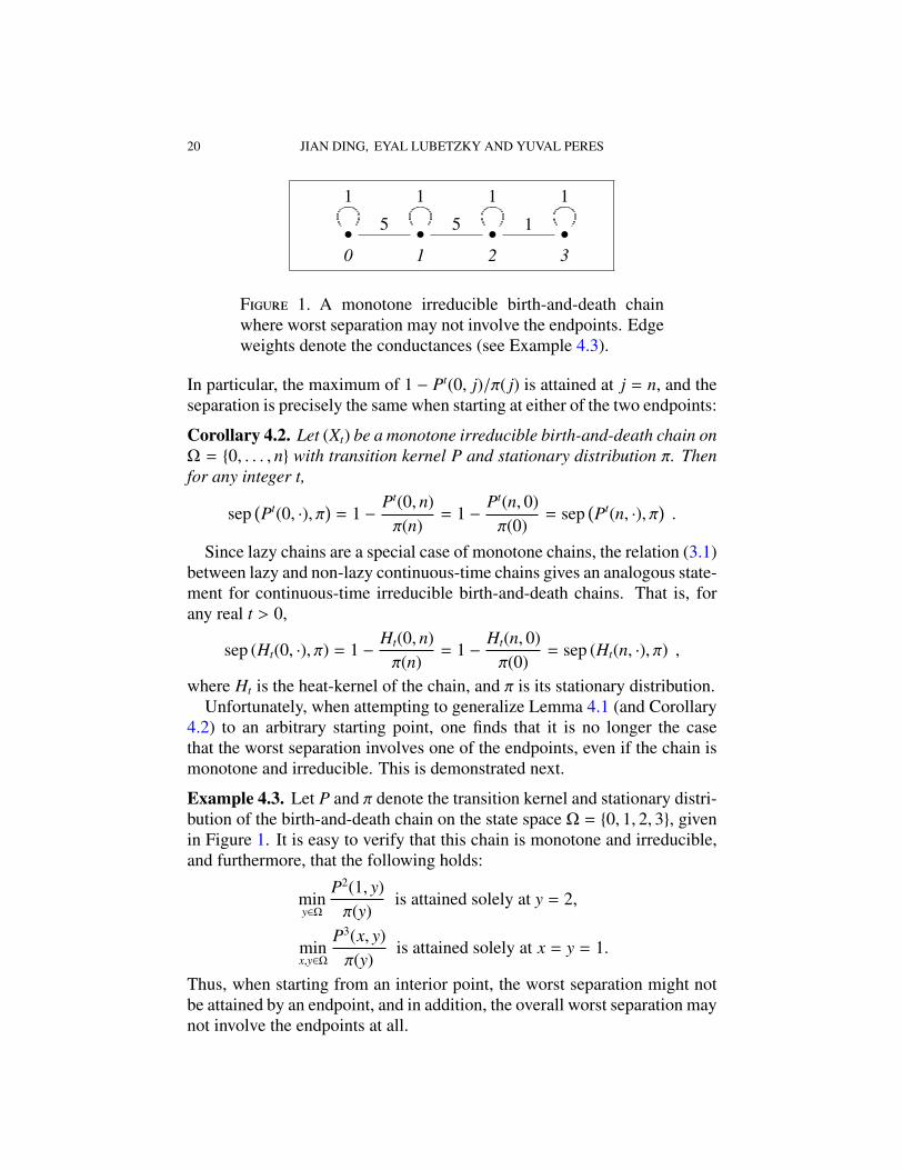
F 1. A monotone irreducible birth-and-death chainwhere worst separation may not involve the endpoints. Edgeweights denote the conductances (see Example 4.3).

In particular, the maximum of 1 − Pt(0, j)/π( j) is attained at j = n, and theseparation is precisely the same when starting at either of the two endpoints:

Corollary 4.2. Let (Xt) be a monotone irreducible birth-and-death chain onΩ = 0, . . . , n with transition kernel P and stationary distribution π. Thenfor any integer t,

sep(Pt(0, ·), π

)= 1 −

Pt(0, n)π(n)

= 1 −Pt(n, 0)π(0)

= sep(Pt(n, ·), π

).

Since lazy chains are a special case of monotone chains, the relation (3.1)between lazy and non-lazy continuous-time chains gives an analogous state-ment for continuous-time irreducible birth-and-death chains. That is, forany real t > 0,

sep (Ht(0, ·), π) = 1 −Ht(0, n)π(n)

= 1 −Ht(n, 0)π(0)

= sep (Ht(n, ·), π) ,

where Ht is the heat-kernel of the chain, and π is its stationary distribution.Unfortunately, when attempting to generalize Lemma 4.1 (and Corollary

4.2) to an arbitrary starting point, one finds that it is no longer the casethat the worst separation involves one of the endpoints, even if the chain ismonotone and irreducible. This is demonstrated next.

Example 4.3. Let P and π denote the transition kernel and stationary distri-bution of the birth-and-death chain on the state space Ω = 0, 1, 2, 3, givenin Figure 1. It is easy to verify that this chain is monotone and irreducible,and furthermore, that the following holds:

miny∈Ω

P2(1, y)π(y)

is attained solely at y = 2,

minx,y∈Ω

P3(x, y)π(y)

is attained solely at x = y = 1.

Thus, when starting from an interior point, the worst separation might notbe attained by an endpoint, and in addition, the overall worst separation maynot involve the endpoints at all.


However, as we next show, once we replace the monotonicity require-ment with the stricter assumption that the chain is lazy, it turns out that theabove phenomenon can no longer occur.

The approach that led to the following result relied on maximal couplings(see, e.g., [19], [22] and [18], and also [23, Chapter III.3]). We provide astraightforward proof for it, based on an inductive argument.

Lemma 4.4. Let P be the transition kernel of a lazy birth-and-death chain.Then for any unimodal non-negative f : Ω → R+, the function P f is alsounimodal. In particular, for any integer t, all columns of Pt are unimodal.

Proof. Let pi, qi and ri be the birth, death and holding probabilities ofthe chain respectively, and for convenience, define f (i) to be 0 for i ∈ N\Ω.Let m ∈ Ω be a state achieving the global maximum of f , and set g = P f .

For every 0 < x < m, the unimodality of f implies that

g(x) = qx f (x − 1) + rx f (x) + px f (x + 1)≥ qx f (x − 1) + (1 − qx) f (x) ,

and similarly,

g(x − 1) = qx−1 f (x − 2) + rx−1 f (x − 1) + px−1 f (x)≤ (1 − px−1) f (x − 1) + px−1 f (x) .

Therefore, by the monotonicity of the chain, we deduce that g(x) ≥ g(x−1).The same argument shows that for every m < y < n we have g(y) ≥ g(y+1).

As g is increasing on 0, . . . ,m − 1 and decreasing on m + 1, . . . , n,unimodality will follow from showing that g(m) ≥ min g(m − 1), g(m + 1)(the global maximum of g would then be attained at m′ ∈ m− 1,m,m + 1).To this end, assume without loss of generality that f (m−1) ≥ f (m+1). Thefollowing holds:

g(m) = qm f (m − 1) + rm f (m) + pm f (m + 1)≥ rm f (m) + (1 − rm) f (m + 1) ,

and

g(m + 1) = qm+1 f (m) + rm+1 f (m + 1) + pm+1 f (m + 2)≤ qm+1 f (m) + (1 − qm+1) f (m + 1) .

Thus, the laziness of the chain implies that g(m) ≥ g(m+1), as required.

By reversibility, Lemma 4.4 has the following corollary:

Corollary 4.5. Let (Xt) be a lazy and irreducible birth-and-death chainon the state space Ω = 0, . . . , n, with transition kernel P and stationarydistribution π. Then for any s ∈ Ω and any integer t ≥ 0, the functionf (x) := Pt(s, x)/π(x) is unimodal.


Remark. The maximum of the unimodal function f (x) in Corollary 4.5 neednot be located at x = s, the starting point of the chain. This can be demon-strated, e.g., by the biased random walk.

Proposition 4 will immediately follow from the above results.

Proof of Proposition 4. We begin with the case where (Xt) is a lazy birth-and-death chain, with transition kernel P. Let s ∈ Ω be a starting positionwhich maximizes dsep(t). Then by Corollary 4.5, dsep(t) is either equal to1 − Pt(s, 0)/π(0) or to 1 − Pt(s, n)/π(n). Consider the first case (the secondcase is treated by the exact same argument); by reversibility,

dsep(t) = 1 −Pt(0, s)π(s)

≤ 1 −Pt(0, n)π(n)

,

where the last inequality is by Lemma 4.1. Therefore, the endpoints of Xassume the worst separation distance at every time t.

To show that dsep(t) = 1−Ht(0, n)/π(n) in the continuous-time case, recallthat

Ht(x, y) = Px(Xt = y) = E[PNt(x, y)

]=

∑k

Pk(x, y)P(Nt = k) ,

where P is the transition kernel of the corresponding discrete-time chain,and Nt is a Poisson random variable with mean t. Though Pk has unimodalcolumns for any integer k, a linear combination of the matrices Pk does notnecessarily maintain this property. We therefore consider a variant of theprocess, where Nt is approximated by an appropriate binomial variable.

Fix t > 0, and for any integer m ≥ 2t let N′t (m) be a binomial randomvariable with parameters Bin(m, t/m). Since N′t (m) converges in distributionto Nt, it follows that H′t (m) := E

[PN′t (m)

]converges to Ht as m→ ∞. Writing

N′t (m) as a sum of independent indicators Bi : i = 1, . . . ,m with successprobabilities t/m, and letting Q :=

(1 − t

m

)I + t

m P, we have

H′t (m) = E[P

∑mi=1 Bi

]= Qm .

Note that for every m ≥ 2t, the transition kernel Q corresponds to a lazybirth-and-death chain, thus Lemma 4.4 ensures that H′t (m) has unimodalcolumns for every such m. In particular, Ht = limm→∞ H′t (m) has unimodalcolumns. This completes the proof.

Proof of Corollary 5. By Theorem 3, total-variation cutoff (from the worststarting position) occurs iff t = o

(t(1

4 )). Combining Proposition 4 with

[10, Theorem 5.1] we deduce that separation cutoff (from the worst startingpoint) occurs if and only if t = o

(tsep(1

4 ))

(where tsep(ε) = maxx tsep(ε; x)is the minimum t such that maxx sep(Ht(x, ·), π) ≤ ε).


Therefore, the proof will follow from the well known fact that tsep(14 ) and

t( 14 ) have the same order. One can obtain this fact, for instance, from

Lemma 7 of [4, Chapter 4], which states that (as the chain is reversible)

d(t) ≤ dsep(t) , and dsep(2t) ≤ 1 −(1 − d(t)

)2,

where d(t) := maxx,y∈Ω

∥∥∥Px(Xt ∈ ·) − Py(Xt ∈ ·)∥∥∥

TV. Combining this with

the sub-multiplicativity of d(t), and the fact that d(t) ≤ d(t) ≤ 2d(t) (seeDefinition 3.1 in [4, Chapter 4]), we obtain that for any t,

d(t) ≤ dsep(t) , and dsep(8t) ≤ 2d(4t) ≤ 32 (d(t))4 .

This in turn implies that 18 tsep( 1

4 ) ≤ t(14 ) ≤ tsep(1

4 ), as required.

5. C

• As stated in Corollary 5, our results on continuous-time birth-and-death chains, combined with those of [10], imply that cutoff in total-variation distance is equivalent to separation cutoff for such chains.This raises the following question:

Question 5.1. Let (X(n)t ) denote a family of irreducible reversible

Markov chains, either in continuous-time or in lazy discrete-time.Is it true that there is cutoff in separation iff there is cutoff in total-variation distance (where the distance in both cases is measuredfrom the worst starting position)?

• One might assume that the cutoff-criterion (1.4) also holds for closevariants of birth-and-death chains. For that matter, we note thatAldous’s example of a family of reversible Markov chains, whichsatisfies t(n)

= o(t(n)(1

4 ))

and yet does not exhibit cutoff, can be writ-ten so that each of its chains is a biased random walk on a cycle. Inother words, it suffices that a family of birth-and-death chains per-mits the one extra transition between states 0 and n, and already thecutoff criterion (1.4) ceases to hold.

• Finally, it would be interesting to characterize the cutoff criterion inadditional natural families of ergodic Markov chains.

Question 5.2. Does (1.4) hold for the family of lazy simple randomwalks on vertex transitive bounded-degree graphs?

A

We thank Persi Diaconis, Jim Fill, Jim Pitman and Laurent Saloff-Costefor useful comments on an early draft.


R

[1] D. Aldous, Random walks on finite groups and rapidly mixing Markov chains, Semi-nar on probability, XVII, 1983, pp. 243–297.

[2] D. Aldous, American Institute of Mathematics (AIM) research workshop “SharpThresholds for Mixing Times” (Palo Alto, December 2004). Summary available athttp://www.aimath.org/WWN/mixingtimes.

[3] D. Aldous and P. Diaconis, Shuffling cards and stopping times, Amer. Math. Monthly93 ( 1986 ), 333–348.

[4] D. Aldous and J. A. Fill, Reversible Markov Chains and Random Walks on Graphs.In preparation, http://www.stat.berkeley.edu/˜aldous/RWG/book.html.

[5] G.-Y. Chen, The cut-off phenomenon for finite Markov chains, Ph.D. dissertation,Cornell University (2006).

[6] G.-Y. Chen and L. Saloff-Coste, The cutoff phenomenon for ergodic Markov pro-cesses, Electronic Journal of Probability 13 (2008), 26–78.

[7] P. Diaconis, The cutoff phenomenon in finite Markov chains, Proc. Nat. Acad. Sci.U.S.A. 93 (1996), no. 4, 1659–1664.

[8] P. Diaconis and J. A. Fill, Strong stationary times via a new form of duality, Ann.Probab. 18 (1990), no. 4, 1483–1522.

[9] P. Diaconis and L. Miclo, On times to quasi-stationarity for birth and death processes.preprint.

[10] P. Diaconis and L. Saloff-Coste, Separation cut-offs for birth and death chains, Ann.Appl. Probab. 16 (2006), no. 4, 2098–2122.

[11] P. Diaconis and M. Shahshahani, Generating a random permutation with randomtranspositions, Z. Wahrsch. Verw. Gebiete 57 (1981), no. 2, 159–179.

[12] J. Ding, E. Lubetzky, and Y. Peres, The mixing time evolution of Glauber dynamicsfor the Mean-field Ising Model. preprint.

[13] J. A. Fill, The passage time distribution for a birth-and-death chain: Strong stationaryduality gives a first stochastic proof. preprint.

[14] J. A. Fill, On hitting times and fastest strong stationary times for skip-free chains.preprint.

[15] P. R. Halmos, Finite-dimensional vector spaces, Springer-Verlag, New York, 1974.[16] S. Karlin and J. McGregor, Coincidence properties of birth and death processes,

Pacific J. Math. 9 (1959), 1109–1140.[17] J. Keilson, Markov chain models – rarity and exponentiality, Applied Mathematical

Sciences, vol. 28, Springer-Verlag, New York, 1979.[18] S. Goldstein, Maximal coupling, Z. Wahrsch. Verw. Gebiete 46 (1978/79), no. 2, 193–

204.[19] D. Griffeath, A maximal coupling for Markov chains, Z. Wahrsch. Verw. Gebiete 31

(1975), 95–106.[20] D. A. Levin, M. Luczak, and Y. Peres, Glauber dynamics for the Mean-field Ising

Model: cut-off, critical power law, and metastability. to appear.[21] D. A. Levin, Y. Peres, and E. Wilmer, Markov Chains and Mixing Times, 2007. In

preparation.[22] J. W. Pitman, On coupling of Markov chains, Z. Wahrsch. Verw. Gebiete 35 (1976),

no. 4, 315–322.[23] T. Lindvall, Lectures on the coupling method, Wiley Series in Probability and Math-

ematical Statistics: Probability and Mathematical Statistics, John Wiley & Sons Inc.,New York, 1992. A Wiley-Interscience Publication.


[24] Y. Peres, American Institute of Mathematics (AIM) research workshop “SharpThresholds for Mixing Times” (Palo Alto, December 2004). Summary available athttp://www.aimath.org/WWN/mixingtimes.

[25] L. Saloff-Coste, Random walks on finite groups, Probability on discrete structures,2004, pp. 263–346.

J DD S, UC B, B, CA 94720, USA.

E-mail address: [email protected]

E LM R, OMW, R, WA 98052-6399, USA.


Y PM R, OMW, R, WA 98052-6399, USA.


Documents

TOTAL VARIATION CUTOFF IN BIRTH-AND-DEATH …eyal/papers/birthdeath.pdfducible birth-and-death chains, as well as for -lazy discrete chains (where P(x;x) for all x 2). In what follows,