Embed Size (px)
DESCRIPTION
Total
Citation preview


EDITORIAL
No company can survive in today’s competitive world without an ongoing effort to create new products, develop new processes and meet new expectations.

3February 2012 / TechnoHUB 2
Senior Vice President Strategy, Business Development, R&D
We have brought together in this edition a selection of the best articles written by Total experts and published over the last two years by the main international industry associations, such as SPE and EAGE, and in reputed journals such as First Break, Offshore Magazine, Oil & Gas Journal or the Journal of Petroleum Technology.
Technical papers are organized in six categories: HSE, geology, geophysics, reservoir, drilling & wells and field operations, reflecting the path followed by development of an oil or gas field from exploration to production. To provide a more comprehensive picture of Total’s activities, these technical aspects are supplemented with details of the human resources strategy that underpins our extensive technical expertise.
The focus in TechnoHUB is, naturally, on innovation. No company can survive in today’s competitive – and changing – world without an ongoing effort to create new products, develop new processes and meet new expectations. Total’s growth strategy relies to a great extent on innovation and has three main thrusts:
TechnoHUB magazine is an opportunity to showcase the wealth of exploration and production expertise – technical know-how, project management experience and sustainable development initiatives – that Total can offer its partners and co-venturers.
Olivier CLERET de LANGAVANT
▪ Maximizing our existing production – limiting the natural decline of our fields by improving recovery and maintaining the integrity of facilities
▪ Bringing our projects on stream on schedule and at the best cost.
▪ Continually renewing our reserves – acquiring new acreage; targeting new geological frontiers for a bold exploration; sharing our expertise in alliances with new partners, and
Total has ambitious growth targets: to add 1.4 billion barrels of reserves per year, increase production by an average of 2.5% each year, and maintain at least 12 years of 1P reserves and 20 years of 2P reserves. The key to achieving this growth, which must be both profitable and sustainable, is cost-effective technology. That is what TechnoHUB is all about. We hope you find our magazine stimulating.

GEOPHYSICS
58 Velocity model building with wave equation migration: the importance of wide azimuth input, versatile tomography, and migration velocity analysis
68 Impact of modelling shallow channels on 3D prestack depth migration, Elgin-Franklin fields, UKCS
78 3D modelling-assisted interpretation: a deep offshore subsalt case study
4 TechnoHUB 2 / February 2012
HSE
26 New ways to monitor offshore environments - A look at four novel methods and their advantages
58/85STRATEGIC
6 Total Spreads Its Wings
14 Arctic may reveal more hydrocarbons as shrinking ice provides access
21 Total ups Angola content, maximizes gas for latest ‘cluster’ projectMultiphase pumps to drive out heavy Miocene crude
6/25GEOLOGY
32 The whys and wherefores of the SPI−PSY method for calculating the world hydrocarbon yet-to-find figures
46 Borehole image logs for turbidite facies identification: core calibration and outcrop analogues
26/31 32/57
CONTENTS

FIELD OPERATIONS
110 Subsea intervention system for arctic and harsh weather
DRILLING & WELLS
102 Advanced Drilling in HP/HT: The TOTAL Experience on Elgin/Franklin (North Sea – UK)
HUMAN RESSOURCES
116 Geoscience careers at Total
120 Yves-Louis Darricarrère President, Exploration & Production, Total
RESERVOIR
86 Polymer Injection in a Deep Offshore Field — Angola, Dalia/Camelia Field Case
92 4D pre-stack inversion workflow integrating reservoir model control and lithology supervised classification
5February 2012 / TechnoHUB 2
Edition: February 2012 //
TECHNOHUBTotal’s Exploration-Production techniques [email protected] //
Publication Manager A. Hogg / Editor-in-chef V. Lévêque assisted by V. Rogier (Rythmic communication) / Editing committee G. Bouriot, P. Breton, Ph. Julien, D. Le Vigouroux, M. Maguérez, F. Mombrun, P. Montaud, D. Pattou, L. Stéphane / Special thanks to the authors of the Contexts J. Arnaud, F. Audebert, J.L. Bergerot, J.J. Biteau, J.B. Joubert, P. Julien, B. Kampala, F. Larrouquet, V. Martin, P. Mauriaud, D. Morel, J.C. Navarre, E. Rambaldi, N. Tito, S. Toinet / Authorizations for republication obtained from First Break, JPT, Oil & Gas Journal, Offshore Magazine, The Way Ahead, Recruitment / Translation A. Frank / Design and production Bliss agence créative //
ISSN 2257-669X
86/101 102/109 110/115 116/122

6 TechnoHUB 2 / February 2012
Total Spreads Its Wings John SHEEHAN, JPT Contributing Editor
Integrated French energy giant Total is continuing to spread its wings as it focuses on liquefied natural gas (LNG), deep offshore developments, and heavy oil. The Company is seeking to maximize production from its existing fields, while at the same time boosting output from a raft of new projects it is bringing on stream over the next 5 years.
Total has ambitious plans to grow oil and gas output by 2% per year and it is trying to strengthen its upstream arm through exploration, partnerships, and targeted asset deals.
Total is the fifth-largest publicly traded integrated international oil and gas company in the world and is divided into three business segments−Upstream, Downstream, and Chemicals. It produces oil and gas in more than 30 countries, including Angola, Australia, Nigeria, Algeria, Canada, China, Russia, and Qatar.
Editor’s note: This is the fourth in a series of profiles of leading operators, including key international and national oil companies, around the globe. The focus is on the Company’s strategic direction, relationship to its government, major upstream activity, and significant technology challenges and applications.
STRATEGIC
EXTRACTJournal of Petroleum TechnologyDecember 2010

7February 2012 / TechnoHUB 2
Site of the Total-led Yemen LNG plant.
Production of liquids and natural gas was 2.36 million BOEPD in the second quarter of this year, up 8% from the second quarter 2009, while total 2009 output was 2.28 million BOEPD. The Company estimates that the share of gas in production will increase from 44% in the first half of 2010 to 46% in 2014.
Yves-Louis Darricarrère, president of Total’s Exploration & Production Division, said: “Total E&P wants to grow profitably and be one of the best of the majors. To achieve this objective, Total must maximize production from existing fields. This is being done by improving recovery rates from mature fields and by extending production plateaus. Technology and investment are the keywords here.”
He said the Company plans to bring on stream a large portfolio of projects and that startups between 2010 and 2015 will account for 880,000 BOEPD of production (i.e., approximately 33% of Total’s production in 2015).
The main startups between 2011 and 2014 include Trinidad Block 2C, Islay in the North Sea, Usan and Ofon 2 offshore Nigeria, Halfaya in Iraq, Angola LNG, Bongkot South in the Gulf of Thailand, and Kashagan Phase 1 in the Caspian Sea off Kazakhstan.
“We must also focus on reserves replacement,” he added. “This means renewing Total’s portfolio by focusing on organic growth (ongoing exploration, access to discovered resources opportunities awaiting development), and completing it with selective acquisitions.”
ORGANIC GROWTH
Total’s chairman and chief executive officer, Christophe de Margerie, echoed this focus on organic growth: “If we can do more on exploration, we will do it, and for the time being we have decided to increase our exploration budget from USD 1.9 billion in 2010 to USD 2.2 billion in the years to come. We definitely need to be a bit more aggressive and to take a little bit more risk, which means being in frontier exploration areas as well as in the traditional ones.”
As well as expanding its hydrocarbon exploration and production activities around the world, Total is also strengthening its position as one of the global leaders in the natural-gas and LNG markets. The Company is also expanding its energy offerings and “developing complementary next-generation energy activities” including solar, biomass, and nuclear.
Downstream, Total is seeking to adapt its refining system to market changes while consolidating its position in Europe and expanding its positions in the Mediterranean basin, Africa, and Asia.
Total’s chemicals activities will also continue to be developed, particularly in Asia and the Middle East.
In its core upstream sector, Total is launching a raft of projects over the next few months and years.
Some of those are already under construction, including Pazflor, Usan, Angola LNG, and Kashagan, while others such as the West of Shetlands Laggan-Tormore project, the Surmont Phase 2 heavy-oil project in Canada, and the CLOV (Cravo, Lirio, Orquidea, Violeta) deep project offshore Angola are all coming off the drawing board this year.
And it is on Angola’s Pazflor that Total will be showcasing some of the new technology that it has been working on. Pazflor will be the world’s first development to implement large-scale seafloor gas/liquid separation and pumping. “Pazflor paves the way for technologically feasible, economically viable access to increasingly hard-to-produce oils,” said Darricarrère.
He said another deep offshore challenge is to develop small satellite fields located far from production facilities, and other resources lying in deep, inhospitable waters.

8 TechnoHUB 2 / February 2012
AFRICA THE KEY
A look at Total’s major upcoming projects gives some idea of the importance of Africa to the Company’s overall plans. In 2009, Total E&P equity production in Africa averaged close to 750,000 BOEPD, accounting for 33% of the Group’s total production.
“Africa is one of the main focuses for growth in Total’s production,” Darricarrère explains. Most of the projects there in which Total is involved are operated by the Group. Most of Total’s E&P operations are historically located in the Gulf of Guinea−especially Nigeria and Angola−and in North Africa.”
He said Total has also recently strengthened ties with other African countries, enabling the Group to acquire new exploration permits. “Being awarded operatorship on Block 4 brought Total back to Egypt in 2009 to seek agreements with third parties which have discovered resources but not yet developed them such as the case of Uganda this year.”
Deepwater developments are one of Total’s foremost areas of growth in Africa: Usan, Akpo, and Egina in Nigeria, and Pazflor and CLOV in Angola are some examples of Total’s major current deep offshore projects.
The overall development plan for CLOV uses technologies that have already proven effective on Girassol, Dalia, and Pazflor.
FOCUS ON LNG
The deep offshore Block 17 is Total’s main asset in Angola and the Group also operates the ultradeep offshore Block 32, in which it holds a 30% stake.
In addition, Total holds a 13.6% stake in the Angola LNG project for the construction of a liquefaction plant near Soyo, designed to help monetize the country’s natural-gas reserves. The plant, which is under construction with production expected to begin in 2012, will be supplied by the associated gas coming firstly from the fields on Blocks 0, 14, 15, 17, and 18.
Gas produced on CLOV will contribute as feedstock to the plant, which is just one of Total’s LNG developments around the world. The Company is now the second-largest LNG operator globally.
Production from the second train of the USD 4.5-billion Yemen LNG natural - gas liquefaction plant began in April this year. Combined with output from the first train, the plant can produce 6.7 million tons of LNG per year, equivalent to a hundred cargoes to be delivered each year over 25 years. A 320-km gas pipeline carries feed gas from Block 18 in central Yemen’s Marib region to the Balhaf liquefaction plant on the country’s southern coast.
Further highlighting its passion for LNG, Total in September signed a USD 750-million agreement with Santos and Petronas to acquire a 20% interest in the Gladstone LNG (GLNG) project in Australia. The project consists of extracting coal-seam gas from the Fairview, Arcadia, Roma, and Scotia fields, located in the Bowen-Surat basin in Queensland, eastern Australia. The fields’ resources are estimated at more than 9 Tcf of gas.
STRATEGIC
“To face this challenge Total is leveraging its cutting-edge expertise in subsea processing and all-electric systems (long-distance power transmission and distribution, electrical reheating, command- control of the process and wells), with innovative development projects offering multiphase subsea transport over long distances of more than 100 km.
“With regard to the reliability and integrity of subsea installations, innovative and cost-effective subsea tools are necessary in order to optimize intervention maintenance and repair.
“Total has developed the Swimmer, the first autonomous underwater vehicle that integrates a light world-class ROV [remotely operated vehicle], designed to provide intervention maintenance and repair without a support vessel and for long-term subsea deployment without maintenance. This unit has potential applications on the prolific, Total operated Block 17, offshore Angola.”
A total of 34 subsea wells will be tied back to the CLOV floating production, storage, and offloading (FPSO) unit, which will have a processing capacity of 160,000 B/D and a storage capacity of approximately 1.8 million bbl. The CLOV FPSO, through a unique processing and storage system, will produce two types of oil: one with a 32–35°API gravity from the Oligocene reservoirs (Cravo-Lirio) and the other, more viscous, with a 20–30°API gravity from the Miocene reservoirs (Orquidea-Violeta).

9February 2012 / TechnoHUB 2
MORE LNG
The GLNG project will develop these fields up to a production plateau of 150,000 BOEPD and the project also includes transporting the production over approximately 400 km to a gas liquefaction plant in the industrial port of Gladstone, northeast of Brisbane, on the eastern coast of Australia.
The GLNG liquefaction plant will consist of two trains with a total production capacity of 7.2 million tonnes a year. Startup date for the first train is scheduled for 2014. The LNG plant is expected to reach its plateau production in 2016 for more than 20 years.
“In line with the Group’s strategy to develop new types of partnerships, Total is teaming up with Santos for its expertise in gas production in Australia and with state-owned Malaysian oil and gas company Petronas for its experience in marketing LNG in Asia,” said de Margerie. “Total will bring to the project its experience in successfully managing major projects such as the construction of gas-liquefaction plants, and its capacity to market LNG to the Asian market.”
As a wave of new LNG projects, including Ichthys in Australia and Shtokman Phase 1, come on stream, Total wants to bump up its LNG output by 200,000 BOEPD by 2020. The Company is also expanding its activities in unconventional gas and has a 25% stake in the Barnett Shale Joint Venture with Chesapeake in the US. It also has shale-gas exploration permits in France, Denmark, and Argentina.
TOTAL GETS HEAVY
Highlighting the diversity of its operations around the world, Total is also involved in the production of heavy-oil reserves in Canada and Venezuela.
In Canada, the Company operates the Joslyn and Northern Lights leases and is a partner in the Surmont project, all located in the province of Alberta. It is also a partner in the Fort Hills project as well as operator of the Bemolanga license in Madagascar and a partner in the Qarn Alam and Mukhaizna fields in Oman.
ProjectIslayPazfl orUsanHalfayaAngola LNGKashagan Phase 1
Ofon 2SuligeCLOVLaggan/TormoreEkofi sk SouthGLNG
CountryUKCSAngolaNigeriaIracqAngolaKazakhstan
NigeriaChinaAngolaUKCSNorwayAustralia
TypeGas / condesateDeep offshoreDeep offshoreLiquidsLNGLiquids
LiquidsGasDeep offshoreDeep offshoreLiquidsLNG
15220180535175300
7050
1609050
150
100%40%20%20%
13.6%16.8%
40%100%40%80%
39.9%20%
Capacity (kboe/d) Total’s Share
MAJOR PROJECTS TO 2012

10 TechnoHUB 2 / February 2012
The Rosa project launched in 2004 and is located deepwater offshore Angola.
STRATEGIC
On the Surmont lease, 27,000 B/D of bitumen are produced using steam-assisted gravity drainage (SAGD). Two parallel horizontal wells, a production well at the base of the reservoir paired with a steam-injection well 5 m above it, are drilled. Heated by the steam, the less-viscous bitumen flows by gravity down to the production well.Developed in phases, the Surmont lease will see its production rise to 100,000 B/D in Phase 2 and 400,000 B/D in the longer run. As Darricarrère explains, improving the environmental footprint and energy efficiency of extra-heavy-oil production is a strategic R&D focus for Total.
The Group is working on several innovative technologies to address the challenges and one example being studied for potential application to extra-heavy oils is the first European field test integrating the complete CO2 capture, transport, and storage chain, in Lacq in southwest France.
“The Lacq field test aims to validate the innovative technology and process before a larger scale industrial deployment is considered. Total is also working on a series of innovative technologies to improve the energy efficiency of the thermal production and upgrading of extra-heavy oil, via, for example, a reduction in the steam/oil ratio, innovative boilers, cogeneration, etc.,” he said.
“In coordination with Total’s R&D center in Pau, France, the research center in Calgary is working on pilot processes which include a solvent- steam coinjection pilot project that may further reduce the amount of steam required in the SAGD process, therefore reducing required water volumes and CO2 emissions.
“For mining projects, the main challenge consists in increasing water recycling, which averages 80% on current projects. Our efforts are directed at safeguarding water resources, recycling at every opportunity and reducing tailings. The Joslyn Mine project has been designed to maximize the water makeup and achieve water consumption that is lower than the industry average.”
Founded: Compagnie Française des Pétroles in 1924 Operations: E&P activities in more than 40 countries Production of oil and gas in 30 countries Production: 2.28 million BOED Proved reserves: 10.5 billion BOE Employs: 96,387 employees Approximately 540,000 French individual shareholders
TOTAL AT A GLANCE
11February 2012 / TechnoHUB 2
Executive Vice President Total,President Total Exploration & Production
Yves-Louis Darricarrère was appointed president of Total Exploration & Production in 2007. He has been a member of Total’s Executive Committee since 2003. From 2003 until 2007, Darricarrère was president, Total Gas & Power. In 2000, he was appointed senior vice president Northern Europe of TotalFinaElf (subsequently Total) Exploration & Production and became a member of the Group’s Management Committee. He joined Elf Aquitaine in 1978 as a design and projects engineer in the Mining Division. He was successively projects engineer for Aquitaine Australia Minerals in Sydney, country representative Australia-Egypt, managing director of subsidiaries in Egypt and Colombia, director of Acreage Assets Negotiations and New Ventures Exploration- Production, chief fi nancial offi cer Oil and Gas and then deputy director of General Exploration & Production, and a member of the Management Committee of Elf Aquitaine. He is a graduate of the École Nationale Supérieure des Mines and the Institut d’Études Politiques in Paris and also has a degree in economics.
Yves-Louis DARRICARRÈRE
Q&AHow does Total’s integrated business model help push the business forward?
In the Upstream,Total has been able to launch major projects on the strength of the synergies between E&P and gas and power. One example of this is Yemen liquefi ed natural gas (LNG), a project developed by the E&P branch and including long-term gas sales agreements binding it to gas and power. Another is Nigeria where the two branches invested jointly in a power-generation project.
Integration between the Upstream and Downstream activities in Total also allows the Group to pursue its development strategy. For instance, in Uganda, Total’s long-standing distribution activities in the country, combined with the positive relationship developed by the local teams with the authorities, paved the way for the expansion of Total E&P activity in Uganda through a partnership involving Total, China’s CNOOC, and Tullow Oil on their exploration assets in the Lake Albert region.
In China, Total’s distribution network and the Group’s willingness to invest in integrated projects—which combine refi ning, petrochemicals, and distribution— led Total to forge strong partnerships with Chinese national oil companies. As it is recognized as being a trustworthy business partner, Total can position its E&P branch as an international partner for national oil companies (NOCs).
Finally, a number of projects led by the Group have the potential to become future business tools spanning the entire range of Total’s activities. The fi eld test for carbon capture, transport, and storage, inaugurated in January at Lacq, southwest France, has generated leads and opportunities for Total to reach the objective of reducing its environmental footprint in all activities.
What is Total’s strategic outlook for the Upstream, and how is that likely to change in the future?
It is estimated that energy demand will increase by approximately 1.2% per year between now and 2030, by which time it will be 26% higher than today. To satisfy that demand, energy supply needs to diversify, although fossil energies should still represent approximately 75% of supply in 2030, compared with 81% today. There are long-term perspectives for the oil and gas industry and abundant resources available, but developing those calls for advanced technology and heavy investments.

12 TechnoHUB 2 / February 2012
developments already under construction such as Pazfl or, Usan, Angola LNG, and Kashagan. Of the fi ve major projects scheduled to kick off in 2010, three are already under way:
▪ Surmont Phase 2 in Canada, with an expected production of 110,000 B/D of heavy oil through a steam-assisted gravity drainage system
▪ The Laggan and Tormore gas fi elds in the North Sea, which lie around 140 km west of the Shetland Islands under 600 m of water. They have total estimated reserves of approximately 230 million BOE and production is to peak at more than 90,000 BOEPD.
▪ Total has very recently announced the development launch of the CLOV deep offshore project in Angola and award of the main contracts. The project involves the production of four development areas (Cravo, Lirio, Orquidea, Violeta) in water depths ranging from 1,100 to 1,400 m. It will simultaneously produce two oils with different characteristics (Oligocene and Miocene oils). For Total, this is the fi rst time that a subsea multiphase pump system will be installed in the deep offshore to boost production.
Two other major projects will be launched later in the coming months in Nigeria: Ofon II, an offshore development with an expected production of 70,000 B/D, and Egina, a major deep offshore project with an expected production of 200,000 B/D.
How is Total likely to continue its international expansion?
The Group’s efforts in acquiring new exploration permits have further expanded its playing fi eld. It has added a number of exploration licenses to its portfolio over the past 6 or 7 months in various promising geological regions in different countries: France, French Guiana, Yemen, Argentina, Brazil, Vietnam, Malaysia, Indonesia, Kazakhstan, and Azerbaijan.
Not only this, but the kinds of partnership we enter into these days have changed –no longer just the traditional joint-venture model between majors – putting us in a better position for international development.
Total supports and accompanies NOCs in their ambition to develop their activities outside their frontiers; this is what we did in partnering with the Chinese company CNPC in Iraq on the Halfaya fi eld and with Qatar Petroleum in Africa.
Oil demand is expected to show a marked increase between 2010 and 2020 in emerging countries or regions, such as in China or the Middle East, but decrease in North America and Europe.
As for gas, the economic crisis has temporarily curbed the regular increase observed in world gas demand. Consumption fell by approximately 1.5% in 2009 compared with 2008.
We expect demand to resume its regular progress from 2010 on, with a dynamic growth rate of more than 2% during 2010–2020. However, this will depend on an increase in unconventional- gas production and the development of LNG, where there is a need for further investment so as to avoid potential shortages.
Finally, as gas production has a lesser impact on the environment than oil production, there will be a natural preference for gas.
What does Total see as its main focus area for the upstream in the future?
While Total continues to invest in conventional hydrocarbons, we also intend to build on positions in highpotential sectors in countries with promising resources. Our portfolio is well-balanced in terms of risks (geographical situations, technologies used, project profi tability) and has consolidated the Group’s strengths, particularly in:
▪ The deep offshore (Congo, Nigeria, Angola) where technology and integrated project management are essential
▪ LNG (Australia, Russia, Nigeria) where integrated project management and upstream/downstream marketing integration, as well as technology, are the keys to success
▪ Heavy oils (Canada, Madagascar) where technology, integration with refi ning, and stewardship of natural resources (water, air, energy, etc.) are mandatory
▪ Complex/unconventional-gas plays such as high-pressure/high-temperature (HP/ HT) (North Sea), tight gas (Algeria), and shale gas (US and applications in Europe) where, again, advanced technology and expertise are required.
What big upstream projects are due on stream and what technology challenges do they present?
Some 40 developments of different sizes and importance will be brought on stream over the next 5 years, some of them being major
STRATEGIC

13February 2012 / TechnoHUB 2
Total also partners with independent companies that possess specifi c technological know-how, as for example in the association with Chesapeake on its shale-gas assets and the partnership with the Russian gas producer Novatek to jointly develop the Termokarstovoye fi eld in its harsh environment.
What is the importance of the Laggan-Tormore project to Total and what challenges do you foresee?
Engineers called the Laggan and Tormore reserves “stranded gas,” reserves too remote or small to make their development economically viable. The West of Shetlands area, on the edge of the UK continental shelf, is thought to contain approximately 17% of the UK’s remaining oil and gas reserves. These are important for future energy supply but, until recently, were stranded under deep and hostile seas.
Total’s interests in this remote and harsh environment are focused around two fi elds: Laggan, located 125 km west of the Shetland Islands, and Tormore, a further 16 km southwest. Both fi elds lie in 600 m of water and hold estimated reserves of 230 million BOE, enough energy to heat every single home in a city the size of Aberdeen for 550 years.
Laggan-Tormore is one of the UK’s biggest infrastructure projects in a decade, with a development cost estimated at £2.5 billion. After Alwyn and Elgin-Franklin, the West of Shetlands area will be Total’s third development hub in the UK and a key to unlocking opportunities in the greater West of Shetlands region for Total and the industry as a whole.
Laggan-Tormore presents two main challenges. One is technical: in this harsh environment, the multiphase subsea tieback to a new plant on Shetland will be one of the longest in the world at 143 km. The other is environmental: the project is located in an area subject to intense environmental scrutiny, as the Shetland Islands are home to sites of specifi c scientifi c interest and a valuable fi shing industry. Finding effective solutions to minimize its environmental footprint is paramount for Total.
What is Total’s current upstream R&D focus?
Total’s R&D programs aim to address the challenges facing the oil and gas industry, namely, how to:
▪ Cost-effectively extend production from our current fi elds, in particular by means of enhanced-oil-recovery technologies to
improve oil recovery using chemicals such as polymers or surfactants. Another focus is to improve Total’s geomodeling technologies and reservoir characterization to understand complex reservoirs and achieve better recovery from carbonate reservoirs, whose production is estimated to represent 45% of worldwide oil production by 2030.
▪ Explore and develop challenging plays including extra-heavy oils and bitumen, deepwater reservoirs, HP/HT deeply buried reservoirs, unconventional resources (shale oil, shale gas, tight gas reservoirs, etc.) by deploying emerging, cost-effective technologies and by improving exploration tools (seismic imaging, geological models). Total has also put in place strategic partnerships in the area of unconventional resources, to develop expertise in atypical production methods for tight reservoirs, heavy-oil production, and oil shales.
▪ Reduce the Company’s environmental footprint and enhance operating safety, with particular focus on extra-heavy oils and bitumen production, as well as on the integrity of its deep offshore installations. Programs on this subject are being reviewed in the light of the recent events in the Gulf of Mexico.
What is Total’s primary focus on technology and what innovations is it working on?
Securing worldwide energy demand involves producing resources that require complex and ground-breaking technologies. Major recent technological advances, as well as those in deepwater and heavy oil, include:
▪ In Angola, the fi rst fi eld tests for deep offshore polymer injection are being carried out in the Dalia reservoirs. Since late 2009, polymer-enhanced water has been injected in the Camelia reservoir via a line that feeds fi ve injection wells. Extending the use of this chemical process to the entire fi eld, planned for 2014, is expected to boost recovery by approximately 5% over 20 years, which means increasing reserves by more than 10%.
▪ On the exploration side, Total is continuing to generate new geophysical processing seismic algorithms to improve seismic imaging. Its teams are developing bits, such as microcoring bits with a good penetration rate and measurement-while-drilling tools capable of resisting temperatures of up to 230°C for 14 consecutive days, and muds (drilling muds that remain stable beyond these temperature thresholds) for improved drilling effi ciency and formation evaluation while drilling in HP/HT deeply buried environments.

14 TechnoHUB 2 / February 2012
STRATEGIC
Arctic may reveal more hydrocarbons as shrinking ice provides accessMarc BLAIZOT - Total SA - ParisCondensed from a presentation at the first Offshore Technology Conference Arctic Conference Feb. 6-9, 2011, in Houston.
Geographically, the Arctic polar regions correspond to the whole of the land and sea area north of the Arctic Circle (66° N. Lat.), roughly from north of Iceland on one side and south of the Bering Strait on the other. It represents around 20 million sq km.
Within the Arctic areas around 400 billion boe has been already discovered, 80% being gas!
The main proved basins and mostly untapped reserves are located in Russia, the Barents Sea, the Kara Sea, and the Yamal Peninsula for gas and in Alaska, the North Slope basin for oil. Others important basins are Timan-Pechora in Russia as well as the MacKenzie Delta and Sverdrup basin in Northern Canada.
EXTRACTOil and Gas JournalMay 2, 2011USD 10

15February 2012 / TechnoHUB 2
Figure 1: Arctic resources and reserves assessments
Figure 2: Geodynamic evolution of Arctic basins in Mesozoic times
Several basins mainly located in Eastern Russia are totally virgin, devoid of any exploratory wells, and are conceived only through neighboring outcroppings as well as sparse 2D seismic lines. They are mainly the offshore North Kara Sea, Laptev Sea, East Siberia platform, and North Chukchi that together represent more than five times the surface area of Texas.
For explorationists, two key questions are:
Why so much gas at a scale unknown in any other region of the world?
Can we find oil in the Arctic and where? The latter question is important, because Arctic gas except in the Yamal Peninsula and Barents Sea could be stranded for long periods.

16 TechnoHUB 2 / February 2012
The only exceptions are clearly Prudhoe Bay and adjacent fields and very rare oil tests such as Goliath in the Barents Sea. There the two excellent marine oil prone sourcerocks have generated an exceptionally high quantity of oil in stacked fluvial channel deposits, sandstone reservoirs of Triassic age. Both Triassic and Jurassic source rocks are within the oil window as exhibited by the maturation indexes.
Other oil discoveries are possible in the offshore part of this basin even if these source rocks are without any doubt much more deeply buried (>5,000 m). But liquids could be present as condensate given the probable high pressure (600 to 800 bars) and nature of the source rock. More than 1 billion bbl of condensate has been calculated on the Dinkum South undrilled area where the excellent Sadlerochit reservoir seems present and thickens from south to north.
The Beaufort Sea basin in Canada is also marked by an important orogenic compressive event in Mid-Tertiary followed by an important prograding Tertiary delta linked to the paleo and present Mackenzie River. Mainly gas discoveries have been found in Tertiary platform or turbiditic sandy reservoirs associated with gas prone source rocks.
Northwards more distal conditions should prevail according to Total’s paleogeographical reconstructions. Therefore oil prone marine source rocks could be encountered. Huge folded structures are present there and should intersect distal channel and levee turbiditic complexes mainly in the Oligo-Eocene series. Therefore both Dinkum and North Beaufort clearly exhibit promising plays for the present decade of exploration.
The Hammerfest basin in northern Norway is well known through the development and production of the most northwards LNG production to date, the Snohvit field complex. But it is above all the perfect example of a basin, rich in excellent marine oil-prone source rocks both in Triassic and above all in Jurassic layers and finally very poor in oil discoveries except for Goliath field on the southern edge of the basin. The Snovhvit complex, however, has been fed with oil as witnessed by the numerous oil shows located below the gas pool in the presently water-bearing zone. Several hypotheses have been contemplated for explaining this result, the first one being the past oil flushed by the subsequent gas generation with consequent oil migrating towards the southern updip basin edge.
ASSESSMENTS OF THE ARCTIC ENDOWMENT
The Arctic Polar Regions owe their principal bathymetric and orographic features to two oceans, the North Atlantic Ocean and the Arctic Ocean (figure 1 p. 15).
The geological organization results from geologically speaking recently created oceanic crusts in Cretaceous times for the Eastern Canadian basins and in early to late Tertiary times for the Atlantic and the Arctic Oceans that have triggered off the separation of the North American plate and the Eurasian plate.
These oceanic openings and continental drifts have been preceded by tectonic tension phases since Middle Triassic, having created rift and graben structures followed by platform sags. This history is similar in a lot of Arctic basins, the differences coming mainly from presence of Tertiary orogenic events north of Alaska and East Siberia.
Such a structural configuration induces four main post-Hercynian petroleum systems linked to four source-rock deposits (figure 2 p. 15):
▪ Late Triassic marine source rocks extended in practically all the known already drilled basins from the Chukchi Sea westward to the Yamal Peninsula eastward.
▪ Late Jurassic exceptionally rich marine source rocks spread over the Barents, West Siberian, Yamal, and probably Kara seas (the well-known Bazhenov source rock) as well as in the North Slope.
▪ Then in Upper Cretaceous marine source rocks are known in North Canadian and North Alaskan basins as well as possibly in western Greenland and Baffin Bay.
▪ And finally, since Oligocene deltaic source rocks, more gas prone, were deposited in big northward-prograding deltas like the Mackenzie and Lena rivers.
When source rocks are superimposed with already discovered fields, an amazing anticorrelation appears between largely predominant marine, oil prone source-rocks and gas fields, implying that mechanisms other than the nature of source rocks are needed to explain the gas discoveries.
STRATEGIC

17February 2012 / TechnoHUB 2
This induced a beginning of hydrocarbon migration southwards and gas expansion due to shallow burial and a decrease of reservoir pressure. But more striking have been the onsets of a thick ice cap associated with permafrost in Quaternary that has increased the pressure at depth particularly of the cap rock inducing important leakage and within the reservoir generating fluid shrinkage. Melting of the ice cap in recent times induced again a pressure decrease and gas expansion and therefore generalized gas caps.
The amplitude of these phenomena of icing and melting has been so huge in Quaternary with so many periods of green and icehouse effect that it has been detrimental to the presence of oil.
As a consequence oil could be found only on the edges of the basins or at very important depth where hydrocarbons always remain in monophasic (critical fluids) phase.
Accordingly where thick ice caps have expanded associated with uplifts and erosion at the edges of the newly created oceans, gas probability will be high. Total has developed a model based on ice pack history allowing to define these gas prone areas (dark blue in figure 3). These regions encompass a large part of the Russian arctic basins, whereas the light blue areas would be more oil prone and mainly located in the US, Canada, and Greenland.
INFLUENCE OF BARENTS SEA UPLIFT
The picture could be more complex if we remember the last several million years’ history of this basin, which underwent a large erosion of more than 1,000 m in Tertiary (figure 3).
Figure 3: Barents sea: infl uence of uplift and ice cap on fl uid preservation

18 TechnoHUB 2 / February 2012
Figure 4: Why so much gas? Direct impact of present Arctic conditions?
Figure 5: Arctic/Frontier basins; expected prevailing fl uids
STRATEGIC
19February 2012 / TechnoHUB 2
THE ARCTIC PREDOMINANCE OF GAS
Geological and ice extension histories, therefore, should permit the forecasting of what could be found even in poorly explored frontier basins.
As an example here is the Kara Sea (figure 4) where two huge gas fields were discovered in the 1980s and presenting however excellent oil prone source rocks in Jurassic seems to be quite similar to the Hammerfest basin. In such a configuration gas should be expected, oil being still possible at the edges of the basins in prospects mapped both northwards and southwards.
The Laptev Sea basin in Eastern Siberia is a frontier basin. It should have both gas and oil-prone source rocks according to Total’s geological interpretations, but there too gas is the most probable fluid as it could be witnessed by the direct hydrocarbon indicators exhibited on the rare seismic lines shot there.
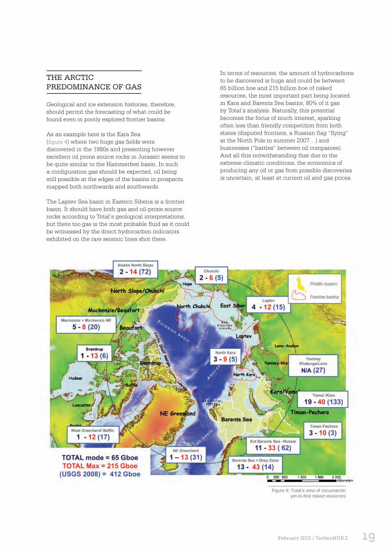
Figure 6: Total’s view of circumarctic yet-to-fi nd risked resources
In terms of resources, the amount of hydrocarbons to be discovered is huge and could be between 65 billion boe and 215 billion boe of risked resources, the most important part being located in Kara and Barents Sea basins, 80% of it gas by Total’s analysis. Naturally, this potential becomes the focus of much interest, sparking often less than friendly competition from both states (disputed frontiers, a Russian flag “flying” at the North Pole in summer 2007…) and businesses (“battles” between oil companies). And all this notwithstanding that due to the extreme climatic conditions, the economics of producing any oil or gas from possible discoveries is uncertain, at least at current oil and gas prices.

20 TechnoHUB 2 / February 2012
PREVAILING FLUIDS AND YET-TO-FIND VOLUMES
Large exploration potential still exists both in prolific and frontier basins, mainly in Russia, where the predominant fluid will be gas by far (figures 5 and 6 p. 18,19).
Oil should be and would be explored for thanks to two main criteria: source rock nature and maturation as well as quaternary icing history.
Exploration will be difficult owing to the exceptional climate conditions, equally hostile to man and equipment.
The inventory of these regions’ oil and gas potential is far from complete. This is due chiefly to lack of seismic acquisition and exploratory drilling, the only techniques capable of verifying at depth the existence of hydrocarbon accumulations, as both are hampered by the frequent presence of pack ice in winter and marshy areas onshore in summer.
Moreover, due to the rich array of flora and fauna—above ground, fresh water or marine conditions with planktonic and-or benthic fauna—highly specific precautions have to be taken in deploying equipment that may prove harmful in the medium term.
PACK ICE SHRINKS TO PERMIT EXPLORATION
Taking into account 30 years’ global warming, it is reasonable to assume that in most of the shallow-water offshore locations in the Arctic surface pack ice coverage will drastically shrink over the next 20 years, even in winter.
This warming is thought to be essentially due to human activity (anthropogenic): the emission of greenhouse gases, the products of pollution generated under latitudes far removed from the Arctic, in industrialized countries.
Even though exploring for and producing hydrocarbons in Arctic regions will cause only an infinitesimal increase in GHGs compared with the emissions from agriculture, industry, or global transport, every possible effort must be made to keep the impact of these activities on the extremely fragile, pristine Arctic environment (in terms of its biodiversity and communities) to an absolute minimum.
In managing these activities, the oil companies and the states bordering the Arctic must therefore treat this environment with the greatest care and attention to detail. Effectively, they are very capable—working in cooperation—of undertaking these highly costly explorations and developments, in coordination with national governmental organizations and local communities.
On this condition, global warming may prove to be a genuine opportunity for growth and sustainable development, for the planet as a whole and for the circumpolar regions in particular.
THE AUTHOR Marc Blaizot is exploration director of Total Exploration & Production. He began as a geologist with Elf Aquitaine in 1979, holding a variety of positions focusing on basin evaluation, prospect generation, and appraisal of discoveries in Italy, Norway, and the UK. Appointed senior vice-president, exploration, in Angola in 1992, he headed the team of geologists and geophysicists that discovered giant Girassol fi eld. From 1996 to 2001, he conducted geoscience analyses for Syria, Iraq, Qatar, and Asia at the Scientifi c and Technical Center in Pau, France. He was appointed senior vice-president, geosciences, in December 2008. He is a graduate of École Nationale de Géologie.
STRATEGIC

21February 2012 / TechnoHUB 2
STRATEGIC
Total ups Angola content, maximizes gas for latest ‘cluster’ projectMultiphase pumps to drive out heavy Miocene crudeJeremy BECKMAN - Editor, Europe
Construction is under way for CLOV, Total’s fourth deepwater development “pole” in block 17 off Angola. The FPSO is being engineered in South Korea and Singapore, and development drilling should in the second half of next year, with first oil set to flow in 2Q 2014.
The project was sanctioned last August, and the timeframe to start-up of 201 weeks is not the quickest for a development of this scale. But that was mainly due to the drive to maximize the content of Angolan fabrication and integration work, which will be higher than on previous block 17 programs.
As with its predecessors Girassol, Dalia, and Pazflor, CLOV will be produced via a centrally located floater with an extensive SURF spread, but there the similarities end. For one thing, nearly all CLOV’s gas will be harnessed from the outset for the Angola LNG (AnLNG) Project, which comes on stream next year. CLOV will also break new ground for Total in the form of subsea multiphase pumping and all-electric power on the FPSO.
EXTRACTOff shoreMay 2011
22 BEST PAPERS / January 2012
2007, when CLOV was designated a project. The team is headed by Project Director Genevieve Mouillerat, who was previously FPSO package manager on Dalia.
At CLOV, however, the Oligocene reservoirs account for three-quarters of the total oil reserves of 505 MMbbl. At 0.5-0.6 cp, this oil is some of the best-quality in block 17, with a gravity range of 32-35°API, a low wax content, and no sulfur. Temperature and pressure is also favorable, in the range 75-80°C (167-176°F) and 300 bar (4,351 psi). CLOV’s Miocene oil, which represents a quarter of the reserves, is more viscous and lower quality, with 20-30°API gravity, with lower reservoir temperatures (around 50°C, or 122°F) and pressure (200 bar, or 2,900 psi).
“The combination is not ideal,” Mouillerat said, “but we can separate the commingled crudes in one topsides train. At Dalia, when the effluent arrived at the FPSO, we had to re-heat it to achieve separation. With CLOV, however, the temperature on exiting the reservoirs is high enough to make this unnecessary.”
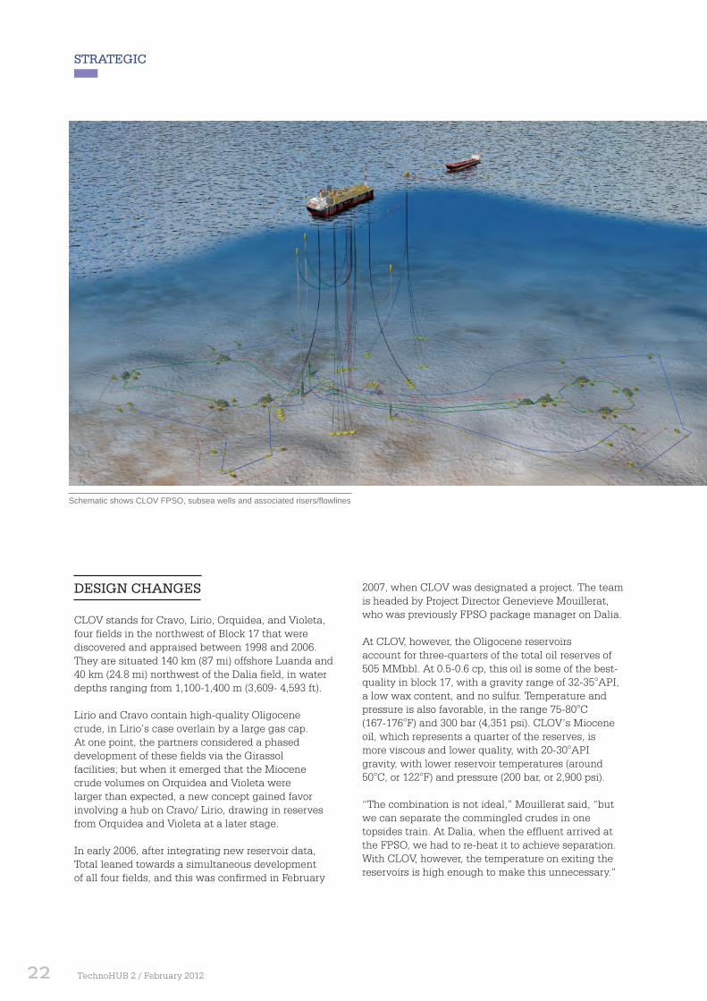
Schematic shows CLOV FPSO, subsea wells and associated risers/fl owlines
DESIGN CHANGES
CLOV stands for Cravo, Lirio, Orquidea, and Violeta, four fields in the northwest of Block 17 that were discovered and appraised between 1998 and 2006. They are situated 140 km (87 mi) offshore Luanda and 40 km (24.8 mi) northwest of the Dalia field, in water depths ranging from 1,100-1,400 m (3,609- 4,593 ft).
Lirio and Cravo contain high-quality Oligocene crude, in Lirio’s case overlain by a large gas cap. At one point, the partners considered a phased development of these fields via the Girassol facilities; but when it emerged that the Miocene crude volumes on Orquidea and Violeta were larger than expected, a new concept gained favor involving a hub on Cravo/ Lirio, drawing in reserves from Orquidea and Violeta at a later stage.
In early 2006, after integrating new reservoir data, Total leaned towards a simultaneous development of all four fields, and this was confirmed in February
STRATEGIC
TechnoHUB 2 / February 2012

23February 2012 / TechnoHUB 2
FLOW ASSURANCE
The four fields are spread, with Lirio and Cravo on one side and Orquidea and Violeta on the other, with distances in between of 9-10 km (5.6-6.2 mi). This introduces thermal and insulation constraints for the interfield flowlines, Mouillerat says. “On the Oligocene reservoirs, our solution is a production loop tying in all the wells – it’s quite a change from the dual-line arrangement on the previous block 17 projects. But the differential pressure for each of the wells will make it challenging for production.” “To address this, we have made available a ring loop going each way. In the middle of the loop, an in-line tee will allow us to add more wells, depending on production performance or if we find more reserves via future exploration.”
PROCESS SPREAD
Daewoo Shipbuilding & Marine Engineering (DSME) is EPSCC contractor for CLOV’s FPSO, which is 305 m long, 61 m wide and 32 m deep (1,000 x 200 x 105 ft). The oil production capacity is 160,000 b/d, compared with 250,000 b/d for Girassol/ Rosa; 240,000 b/d for Dalia; and 220,000 b/d for Pazflor.
KBR is handling detailed engineering design for the topsides, as a subcontractor to DSME. The vessel’s double-sided, singlebottom hull will support topsides with a dry weight of around 34,000 metric tons (37,478 tons), comprising 11 modules. These will include facilities for oil storage of 1.78 MMbbl; water injection at up to 319,000 b/d; gas compression at up to 6.5 MMcm/d; a compact water treatment unit; and a single train for process and storage of the commingled oils. Following two stages of liquid and gas separation, the oil and water will be separated and desalted in wash tanks with fresh water, followed by stabilization in settling tanks.
The FPSO will be able to accommodate a maximum of 240 personnel. In operation, it will be spread moored in 1,291 m (4,235 ft) water depth, with processed oil exported through two 2-km (1.2- mi), 24-in. (61-cm) offloading lines to a 17-m (56- ft) high, 24-in. diameter oil loading terminal, a rotary-table buoy stationed 1 nautical mile (1.85 km) away. Loading data from the buoy will be conveyed back to the FPSO via a fiber optic cable.
Seadrill’s West Gemini, one of two drillships contracted for development drilling on CLOV.
Development drilling will start in 2Q 2012, with two DP drillships – the Pride Africa and Seadrill’s newbuild West Gemini – working in parallel, at an average rate of 60 days per well. Total aims to have 15 wells in place for first oil, with drilling likely to continue through 2016.
Cravo/Lirio will be developed with 10 producer wells grouped via four 12-in. (30.5-cm), four-slot seabed manifolds, and linked together via a 17-km (10.6-mi) production loop comprising 12 and 16-in. (30.5/40.6- cm) pipe-in-pipe, with a bottom gas-lift riser. Two 12-in. water injection lines (24 km, or 14.9 mi, in total) will be connected to nine water injector wells, with these and the production lines gathered together in a single rigid riser tower suspended beside the FPSO.
On Orquidea/Violeta, the configuration will be nine producers grouped together on four 10-in. (25.4-cm), four-slot manifolds. Here there will be 21 km (13 mi) of dual production lines of 10 and 14-in. (25.4/36-cm) pipe-in-pipe for transporting commingled Miocene and Oligocene oils, with a bottom lift gas riser. Six water injectors will be connected to two 10-in. water injection lines (33 km, or 20.5 mi, in total), with one rigid riser tower linking the injection/production lines to the CLOV floater.
CLOV’s gas will head to the new AnLNG plant in Soyo via a single hybrid riser and a 32-km (19.9-mi) export pipeline with a subsea isolation valve connected to a pipeline end manifold in the AnLNG offshore gas-gathering network. In the event of plant unavailability, there will be back-up solutions to re-inject supplies into other fields in block 17.

24 TechnoHUB 2 / February 2012
STRATEGIC
Acergy (now Subsea7) was awarded a $1.2-billion contract to engineer, fabricate, and install the SURF spread. FMC is providing 36 subsea trees, wellheads and controls, all eight manifolds, plus associated tie-in/tooling systems, and workover control systems for the two rigs. Mouillerat describes the subsea production facilities – at least for the Oligocene reservoirs – as conventional, in terms of what Total has done before on block 17, “although we do make improvements as we go along and improve our knowledge of the reservoirs,” he noted. Total opted for riser towers following a design competition. This solution was first devised for Girassol in the late 1990s – the systems there have performed well, she points out. A further consideration was the need to maximize use of Angolan labor – the Sonamet yard has unrivalled experience of assembling and loading out these structures, which are roughly 1,200 m (3,937 ft) high. Compared with the previous structures delivered for Dalia, there will be improvements this time in design/assembly relating to the buoyancy tanks and use of a guide-frame.
Another local organization, Technip’s subsidiary Angoflex, will manufacture CLOV’s 80-km (49.7-mi) network of dynamic and static production and water injection umbilicals at its base in Lobito.
MIOCENE DRIVE
After 18 months to two years of production, the flow of Miocene fluids from Orquidea/Violeta (50,000 b/d) will be boosted by a 28-metric ton (30.9-ton) multi-phase pumping (MPP) system supplied by Framo, which will be installed around 2-3 km (1.2-1.8 mi) from the FPSO. On Pazflor, Total opted for subsea separation and boosting pumps, but multi-phase pumping in a deepwater setting is a first for the Company.
The Orquidea-Violeta MPP system will comprise a pumping station moored to the seabed via a suction anchor. This will contain two helico-axial pumps, one for back-up, operating at 45 bar (652 psi), with shaft power of 1.8 MW transmitted from the FPSO through a 10.6-km (6.5-mi) power and control umbilical. Unlike the equipment on Pazflor, the MPP system will be capable of pumping all effluents, liquids and gas (582 Am3/h), with a gas volume fraction of 53%. The equipment is designed for a 20-year service life in water.
Use of MPP also reduces the need for gas lift on Orquidea/Violeta. With most of CLOV’s associated gas allocated to Angola LNG, there is no scope for gas injection, with only modest amounts of gas set aside for power on the FPSO. “Doing without gas injection saves the cost of one well,” Mouillerat says, “but on the other hand, it’s technologically quite challenging to start production without this – although it is better for the environment. We will never need gas injection on CLOV. We also have a policy of no flaring during normal operating conditions for this project. We have a flare system for safety, but there will be no pilot light, which is again a challenge. Instead, we will have a complex ignition package.”
POWER MANAGEMENT
The FPSO will be fitted with 100 MW of installed power for operations topsides and subsea. GE was awarded a $114-million contract to supply four LM2500 plus G4 SAC aero-derivative gas turbines for power generation, and five process compressors. The latter, like the water injection and multi-phase pumps, will be electrically driven by variable-speed drive (VSD) systems. This will represent a first for an FPSO anywhere, according to the equipment supplier, Converteam.
The Paris-based Company is providing medium voltage drives from its MV7000 range, based on the latest press-pack IGBT (PPI) technology and incorporating a PWM 3-level inverter. According to Converteam, the adjustable PWM patterns and frequency allow for wide-ranging flexibility, i.e. low switching losses, low motor THD (total harmonic distortion), high-frequency operation (up to 300Hz), and negligible amplitude of torque pulsation at the motor shaft. The VSDs are water-cooled, optimizing use of high-capacity diodes and PPI, and operating with very low noise levels. They also occupy less space than aircooled VSDs, with their attendant ventilation/air conditioning equipment.

25February 2012 / TechnoHUB 2
On CLOV, the arrangement will be:
▪ Four 9.6 MW HP compressors fed by MV7609, 24-pulse diode front-end and asynchronous motor (6 kV/1,717 rpm)
▪ One 4.8 MW LP compressor fed by MV7304, 12-pulse diode front end and asynchronous motor (6 kV, 1,717 rpm)
▪ Two 8.7 MW water injection pumps fed by MV7309, 24-pulse diode front end and asynchronous motor (3 kV/1,900 rpm)
▪ Two 2.3 MW subsea multiphase pump units fed by MV7304, 12-pulse diode front-end and asynchronous motor (6 kV/3, 800 rpm).
“The all-electric approach,” Mouillerat explained, “is proven to be easier for production personnel to operate – particularly during early field operations, when there will be regular spells of equipment stopping and starting. In addition, these VSDs will enable us to use exactly and only the required amount of power. And they will help us towards the end of production when our power requirements will be lower.”
Also new for Total is the offshore installation of the Minox de-oxygenation system that DSME has ordered from Grenland Group in Norway for the compact water treatment module, due to be delivered early next year. This will be used to treat 280,000 b/d of seawater for injection. VWS Westgarth in East Kilbride, UK, is supplying an associated ultrafiltration system and a sulfate removal package.
The variable-speed drive confi guration, supplied by Converteam, which will regulate power on the FPSO.
According to Mouillerat, CLOV’s topsides layout is determined by safety needs. “There will be no more space available than on the other block 17 floaters – some areas have been ‘left’ to accommodate future tiebacks, but that is the same for any FPSO. What is different is the location of the settling tank for oil treatment in the hull, which leaves us with more room.”
The other main challenge on this project has been to raise local content to new levels of participation. “All pipe double-jointing line pipe is to be performed in Angola, close to the installation site,” she points out. When the FPSO arrives from South Korea in 2013, it will be moored in a quayside for installation of the water treatment module on the topsides, which will also be fabricated in Angola.
Altogether, Total estimates that CLOV will provide 9 million man-hours of work for Angolans, representing 20% of global cost of the project for local fabrication and assembly. Angolan labor will account for 64,000 metric tons (70,548 tons) of fabrication and assembly – including 7,704 m tons (8,492 tons) for the FPSO – and nearly 60% of the SURF package.
Total E&P Angola operates block 17 with a 40% interest, in partnership with Statoil (23.33%), Esso Exploration Angola (20%), and BP Exploration Angola (16.67%). Sonangol is the concessionaire.

HSE
26 TechnoHUB 2 / February 2012
In general, there is not a broad variety of proven, efficient means of environmental monitoring in the vicinity of offshore oil and gas production facilities. It is often problematic to measure the chemical, physical and biological conditions of the environment in order to control and demonstrate that exploration and production operations are meeting expectations. In recent years, much work has been undertaken to develop new methods to supplement the existing means.
Total R&D, in collaboration with the HSE department, Total E&P Congo, Total E&P Norway, PERL and others, has undertaken a project to test and evaluate several monitoring methods intended to facilitate Total’s compliance with corporate and regulatory monitoring requirements.
This study combined four innovative methods of environmental monitoring, all of which are on the verge of technical validation. These methods were applied concurrently around an oil platform in Congo, and then compared to existing conventional monitoring methods.
The study was called the Super-Monitoring project because for the experimental design, applications of innovative and conventional methods were superimposed upon each other. The objective of the Super-Monitoring project was to compare, validate and better understand how these novel monitoring methods can supplement existing techniques, while providing greater insight into their field of application.
The following article presents an introduction to the various methods applied during the Super-Monitoring program, including foraminiferal assessment, biomarkers, ecotoxicological testing and passive samplers. Another publication planned for 2012 in a peer-reviewed journal will present the results, comparisons and validation of these methods.
CONTEXT
27February 2012 / TechnoHUB 2
New ways to monitor offshore environmentsA look at four novel methods and their advantages
Recent progress in techniques to monitor regular and planned exploration and production discharges offshore is expanding environmental management options for E&P companies. New water column and sediment measurement methods help make possible informed environmental management decisions. Such monitoring methods can be particularly important as E&P companies look to work in sensitive and previously unexplored environments that test the limits of conventional monitoring.
In some cases, tried and true methods have only limited applicability in deepwater operations and arctic projects. Furthermore, emissions from long-term, regular discharges are the subject of increased focus in terms of effects in the sea and in application of the best available treatment technologies.
Marine environmental monitoring can apply to permits and licenses, validation of numerical models, regulatory reporting, and technology selection. Nearly all the environmental management of an offshore installation relies in some way on the data from marine environmental surveys.
For example, the initial state of the seas surrounding a development are monitored for baseline data and, following start-up, monitoring of the sediment and water column is performed periodically to help ensure the good environmental condition. Also, technology selection can be validated, as in the case of a platform in Norway where water treatment engineers used a fish biomarker survey to demonstrate the effectiveness of improved produced water treatment.
Therefore, good, reliable data that represent temporal and spatial variation are needed to meet these and other environmental management needs. However, monitoring in the marine medium is challenging and limitations often restrict the amount of data available.
Benjamin M. KAMPALA - Total E&P
EXTRACTOff shoreNovember 2011

28 TechnoHUB 2 / February 2012
A CHALLENGING ACTIVITY
Environmental monitoring around offshore E&P activities is expensive compared to the equivalent for land based activities. This means monitoring typically yields fewer samples and is performed less often. The principle contributor to cost is logistics, including a vessel from which to conduct activities. Shipping costs to offshore installations, transport, and analytical costs also push up the expense of marine environmental monitoring.
Spatial and temporal heterogeneity of the water column and seabed makes statistical significance of the data and results coming from these studies a challenge. Often the interpretation of monitoring data must rely on observed trends rather than statistically significant datasets. Consider that water column monitoring from a single sampling point may yield entirely different result on consecutive days, merely from a change in direction of ocean current.
Finally, it is not just cost and variability of the sampling zone that creates challenges. Rough seas, deep waters, arctic conditions, difficulty in sampling around an operating platform, bottom hazards such as pipes and risers, all combine to make environmental monitoring in the marine environment a planning challenge. Occasionally, unanticipated delays or errors caused by these complex situations could mean data is lost or costs rapidly increase.
A NEED FOR NEW METHODS
The use of conventional sampling methods at sea persists partly due to the good data they provide, but also in the case of water column analyses, no alternatives have been available until recently.
With changing regulatory, technical, and other data needs, elaborated methods are needed, particularly in new environments like arctic and deep offshore. They should be cheaper and easier to apply. They should provide additional figures against which indices or guidelines may be measured. They also may provide new types of data, such as information about the ecosystem’s condition. To meet these requirements, new methods have been developed and are starting to see wider application.
When attempting to use a new method, advance testing and study are required and may include a bibliography, lab testing, and pilot studies. The parameters to be reported should be well understood and quantifiable to known limits of detection and uncertainty. Equally important are the spatial and temporal time scales for which the data will be considered valid. Whether results are for physical or chemical parameters should be clear as well as their significance to the ecosystem. Finally, it should be understood which environmental compartment results are indicative (water or sediment).
Once a method is well known, the preferred method to pilot a study is a comparative test. The concurrent testing of monitoring methods permits direct comparison of results and thus validation of a method.
CURRENT MONITORING METHODS
Conventional methods of water, benthic sediment, and benthic invertebrate sampling (the conventional sampling methods) are the workhorses of environmental sampling both offshore and onshore (lakes and rivers). They generally are robust and are considered valid by regulators and stakeholders. These monitoring techniques measure concentrations of substances associated with anthropogenic discharges, including PAHs, BTEX, nutrients, salts, and more.
The analysis of water and sediment samples provide data against which indices or guidelines may be compared, and also can be interpreted by biologists to give an idea of the functioning of the ecosystem and indications of perturbation.
The conventional approach of benthic invertebrate sampling provides data for community structure indices used to interpret ecosystem function. Indices such as Shannon’s or density can reveal nutrient deficiency or enrichment. The principle drawbacks are that these methods are costly, time consuming, and do not indicate the short-term response, but rather the response from years of exposure.
HSE

29February 2012 / TechnoHUB 2
FORAMINIFERAL ASSESSMENT
Examples of Foraminifera sampled offshore. 1: Uvigerina peregrina; 2: Nouria polymorphinoides; 3a-b: Bulimina marginat. Scale bars represent 100 μm. (Photo credit: University of Angers)
Foraminiferal assessment and ecotoxicological testing offer alternatives to conventional sediment compartment monitoring.Foraminifera are unicellular protists with a calcareous shell. To conduct a foraminiferal assessment, samples of sediment must be taken at each station. Once aboard the vessel, the samples are preserved and the topmost layer of sediment is retained for analysis. Laboratory analysis consists of sorting, identifying, and counting the individuals found in a given sieve size.
The benefit of foraminiferal assessment over conventional analyses is that one sample offers data from the period prior to operational activities, as well as indications of effects from drilling discharges. The presence of fossil assemblages permits interpretation of historical conditions, while living foraminifera permit interpretation of current conditions. Analyses can be done on small sample volumes, and studies may offer improved statistical representivity of the area. Moreover, the turnover of organisms is faster than benthic sediment and benthic invertebrates, giving a faster response to environmental conditions. Another argument for foraminiferal assessment is that it can be used to sample in extreme conditions (deepwater, arctic environments) where benthic invertebrates are often not present in large numbers.
The analysis is completed by applying the counted individuals, both living at the time of sampling (identifiable by the preserving agent rose Bengal in tissues) and those from deeper layers of sediment which do not absorb the rose Bengal, and thus are known to be dead at the time of sampling. Indices of community structure and trophic function give insight into the presence of opportunist species and those species sensitive to the substances in the drilling discharges. A similar proportion of each species of foraminifera in both the living and deeper, dead fractions, as well as homogenous community structure, indicates no effect from anthropogenic discharges.
The cost of a foraminiferal assessment is roughly the same as a benthic invertebrate assessment, but foraminifera yield data in deepwater and historical data, making it a more cost-effective alternative in certain situations. Whereas foraminiferal assessment is analogous to the techniques and analysis of benthic invertebrates and similar in costs, ecotoxicological testing is different and may be done at lower costs.

30 TechnoHUB 2 / February 2012
PASSIVE SAMPLERS
Another way to sample concentrations in the water column may provide a number of practical and logistical advantages. Passive samplers permit collection of a time-averaged sample of constituents present in the water column. The sample is gathered slowly over several days, weeks, or months. While conventional water column analyses may have low detection limits, a large volume of water would have to be filtered to find adequate concentrations. This is difficult, and even if realized, the results of a high-volume conventional approach would represent only the short time period where water is being pumped and filtered. With passive samplers, the substances that pass through the membrane and integrate into the sampling medium are considered to represent a time averaged concentration for the entire period of immersion (weeks or months). As such, results from passive samplers have good representation of average concentrations.
When an array of passive samplers is deployed around a platform, results can be presented as isopleths of concentrations on a chart. Passive samplers can measure polyaromatic hydrocarbons (PAHs), benzene/toluene/ethylbenzene/xylene (BTEX), metals, and other substances. This can be cost effective. The cost of passive samplers is about the same as for conventional analyses, yet they yield considerably more data. The deployment and retrieval of such samplers may be performed using small craft such as “surfers”. A principle advantage of this method is the eventual ability to provide datasets to validate produced water dispersion models.
A passive sampler being deployed at sea. Passive samplers are used to sample substances in the water over a period of weeks and are capable of measuring PAHs, BTEX, metals, and other substances. (Photo courtesy Total EP)
ECOTOXICOLOGICAL TESTING
Ecotoxicological testing is not new. What is novel is conducting the tests in an easy-to-use manner on sediments in contact with drilling discharges. A feature of ecotoxicological testing is that the sediment samples are tested in a relevant environmental medium on species with ecological relevance. The test gives an idea of disruption to the ecosystem as a whole rather than just the sum of measured chemicals (which leaves out synergistic effects and effects of those compounds not measured).
Ecotoxicity testing of sediment is done by suspending sediment in clean water and adding reference larvae. The presence of altered larval development stages when examined after 24 hours of incubation is the measure of toxicity and relates to the presence of xenobiotics in tested samples. In effect, the toxic response of the organism can be interpreted to give an indication of effect from anthropogenic discharges. An absence of toxicity indications can be interpreted as no effects. The practical and logistical requirements are equivalent to conventional methods, but ecotoxicological testing can be done at no additional cost or complication to a sampling program. Sampling is easy and can be performed wherever benthic sediment samples are collected, which enables a practical evaluation of spatial extension of toxicity. This provides good information at a low cost.
HSE

31February 2012 / TechnoHUB 2
BIOMARKERS
The biomarker approach has advantages that are quite different than the previous methods. Conducting an analysis of biomarkers involves testing tissue samples for physiological changes that occur uniquely as a result of exposure to a given anthropogenic substance – in this case those present in produced water discharges. The biomarker concept works on the premise that observed physiological or molecular changes in marker species, when compared to reference areas, can be interpreted to explain effects on marker species from emissions.
The timescale of response suits recent discharges (hours/days/weeks) rather than the long leads needed for some other methods. The result is a short-term, local adaptation or response of an individual, rather than a long-term population response in the ecosystem.
Sampling methods for biomarker assessment vary depending on study design and the species used as markers. Gathering for tissue samples can be done by caging of fish and mussles, fish traps, or conventional fishing. Tissue samples may include bile, gills, blood or other, and analysis is performed with a high level of analytical precision. Depending on the experimental design of a given biomarker study, results can be interpreted on diverse spatial and temporal timescales and may include considerations about the fish migration and exposure to discharged material.
The principle drawback of the biomarker method is caused by the uncertainty in results arising from confounding factors. The complexities of ecosystems offer many possible sources to activate biomarkers, potentially altering interpretation. However, when properly planned, it is possible to discern biomarker effects resulting from E&P activities and background effects.
The biomarker method has the ability to overcome uncertainty and in doing so, be an example of an application of evidence-based monitoring. Most monitoring methods require an understanding of pathway and causes resulting in a signal being interpreted. Biomarkers accept that pathways between anthropogenic substances and organisms are complex and simply provide a measure of exposure. Thus, a well designed experiment can demonstrate relative levels of exposure by organisms around an offshore platform, but avoid the need for complicated interpretation. No direct causality needs to be established for biomarkers.
ONGOING RESEARCH NEEDED
Further research is needed to improve ease and function of biomarker, as well as other monitoring methods. The monitoring methods presented here exist at different stages of development. Regardless of the stage, ongoing R&D is needed to innovate and continue to prove the effectiveness of environmental monitoring. This may include the application of existing monitoring methods and the new methods together in order to achieve an integrated understanding of the environment. By doing so, the benefits of these techniques and analytical methods can find new applications and be more readily applied. Such integrated understanding could then indicate what should be a most informative and cost efficient approach to regular offshore monitoring in the future.
Also, the changing business needs which spurred development of these novel methods persist. As oil and gas production evolves, so too will the needs and stakes which drive research and investment in new methods. Those methods which respond best to changing stakes should be supported and R&D efforts should preferentially be invested.
New methods offer rigorous and useful alternatives. Already from using foraminiferal assessments, passive samplers, ecotoxicology analysis, and biomarkers, it is clear that important gains have been made in terms of cost effectiveness, spatial and temporal coverage, geographic applicability, and analytical abilities.
ACKNOWLEDGEMENTThe author wishes to thank Jan Fredrik Børseth of IRIS Biomiljø and Francois Galgani of IFREMER for providing comments and input to this document.
The types of analyses that are typically performed include EROD (ethoxyresorufin-O-deethylase) which is a measure of PAH detoxification, analysis for by-products of PAH metabolism, and histopathology. While each of these analyses provides an indication of an effect on tissue, knowing the exact type of PAH that causes the signal is not needed. This means that the method is robust to detect several pathways of effects without needing to know exactly what they are or how anthropogenic substances act on the tissue (and possibly interact with natural substances). Development of these methods has come from several years of study and collaboration among scientists, industry, and regulators.

TECHNICAL
What are the world’s current hydrocarbon reserves? This has always been one of the major questions the oil and gas industry has had to address, and it remains topical today. Indeed, the global economy would like to know the volume of yet-to-find resources to calculate how much fossil energy the planet still has available. Companies like Total are also keen to determine which petroleum provinces should be the focus of their exploration efforts, and where they should target larger hydrocarbon resources. Yet summing the proven, unproven, probable and possible resources is a difficult exercise. Every basin differs by its location, its geometry, its composition and its history. As for the gentle “cooking” of sediments that started millions years ago beneath our feet in the bowels of the Earth, variations in the many intrinsic parameters – temperature, pressure, presence of a trap, permeability, carrier beds serving as drains for hydrocarbon migration, accumulation in sealed reservoirs – all influence the yet-to-find hydrocarbon quantities. Experts have been working on ways to evaluate hydrocarbon resources for many
32 TechnoHUB 2 / February 2012
GEOLOGY
years. Given the wide variations in published estimates (from 275 to 1,469 billion barrels), any other predictions based on these data are rather sketchy. To obtain a more precise appraisal, a tool has been developed to better predict the world’s yet-to-find hydrocarbon figures. It is the result of five years spent studying, comparing data and developing statistics on conventional resources in discovered, prospective and speculative fields in 170 sedimentary basins worldwide. This method is not merely a sum of barrels; it gives access to the source rocks’ production potential according to the type of sedimentary basin using two new numbers, the Source Potential Index (SPI) and the Petroleum System Yield (PSY).
CONTEXT

33February 2012 / TechnoHUB 2
The whys and wherefores of the SPI−PSY method for calculating the world hydrocarbon yet-to-find figuresJean-Jacques BITEAU,1* Jean-Claude HEIDMANN,2 Ghislain CHOPPIN de JANVRY3 and Bertrand CHEVALLIER4 describe a system developed in Total to calculate remaining world reserves in the yet-to-find category.
1 Exploration Coordination and Portfolio Management, Total, Paris / 2 New Ventures Identification, TEPNV, Houston.3 New Ventures, Total, Paris (Retired) / 4 Total E&P, Azerbaijan, Baku / * Corresponding author, Email: [email protected]
This article is the result of five years’ in-house work devoted to defining projected worldwide hydrocarbon yet-to-find figures. For a large number of sedimentary basins, we have evaluated conventional resource volumes comprising discovered fields, individual prospects and leads, and speculative (notional) potential for minimum cases.
We then tried to define a ‘maximum figure’ which can be extracted from the generative capacities of proved and speculative source rocks identified or assumed in a basin. This enables us to calculate generated hydrocarbon volumes using known or modelled source rock maturities. To achieve this, we used our statistics to compare generated versus accumulated hydrocarbons as well as create a petroleum system yield typology and a real scale of figures (which means petroleum systems having different quantitative efficiencies) for various basins, such as compact systems (with a specifically short to very short hydrocarbon migration distance), rifts, foothills, very ancient shelves, etc. Two early case studies illustrate our results on SPI and PSY figures.
The gaps found between our mode and maximum volumes have been analyzed in terms of possible remaining (yet-to-find) resources and discussed for different examples in more than 170 basins worldwide using analogues for petroleum system yields and calculation of maximal figures.
Yet-to-find (YTF) anomalies are discussed particularly with reference to a number of poorly explored frontier basins. Two other case studies present results of YTF figures and describe this method, now routinely implemented by some of our geoscientists.
We first need to recap some of the general definitions and concepts which can be found in different papers, e.g. Biteau et al. (2003); Andreini et al. (2008); Magoon (1988); Magoon and Dow (1994); Magoon and Valin (1994); Perrodon (1992). We then discuss specific definitions and formulae used to obtain our main figures, calculated for 170 basins worldwide in terms of the generative capacity and efficiency of these petroleum systems (see, Biteau et al., 2003).
EXTRACTFirst BreakVol 28Issue 11November 2010

34 TechnoHUB 2 / February 2012
PRELIMINARY DEFINITIONS
Non-renewable (fossil) resources of organic origin (hydrocarbons) can be split into different categories (Biteau et al., 2003):
▪ Solids: coals and bitumens
▪ Liquids: oils and condensates
▪ Gases: natural gas, dry or wet pending upon
▪ Condensate content
These substances can pass through continuous phenomena from one state to another under the effect of changes of pressure, temperature, and chemical conditions. The basic feature of these substances, in their gaseous, liquid, or solid forms, is that they derive from a non-renewable ‘stock’ of ancient life-form vestiges, mostly plants, whose organic matter has undergone major changes over geologic time, through a heating process called organic metamorphism or often called thermal diagenesis. Organic matter is deposited in varying quantities (which will impact their generative capacity) and gradually buried over time by subsidence and the accumulation of sediments above it. The further down the organic matter, the higher the temperature, hence the ‘hydrocarbon kitchen’ effect: hydrocarbons are generated by the gentle ‘cooking’ of a sediment rich in organic material or kerogen (proto-petroleum). This heating is the result of the increased burial depth of the sediment and occurs over a timescale of millions of years. Once generated and expelled
WHAT ARE KEROGENS?
KEROGEN FORMATION
Kerogens correspond to organic matter resulting from the transformation of the continental or marine biomass. About 99% of this biomass will decompose when it sinks to the sea floor or lake/river beds, although the survival rate is higher under anoxic conditions (poor in oxygen with a low bacterial concentration, as bacteria cause organic matter to decompose). Bacterial decomposition can sometimes, however, have a positive effect and generate biogenic hydrocarbon gas (primarily methane) without going through the drawnout process of transformation from kerogen to thermogenic hydrocarbons. Organic matter is made up of cellular organisms of animal or plant origin, which are an integral part of the evolution of life on the planet.
from the source area into a trap, the hydrocarbons may under certain conditions remain in a petroleum trap (a reservoir, a seal, and appropriate geometry) for hundreds of millions of years but may equally well be completely lost during trap alteration.
The prime requirement for the formation of hydrocarbons is the presence of a sedimentary basin in which organic material can be deposited and preserved (source rock) but five additional conditions must be met before a sedimentary basin is transformed into a petroleum province:
▪ Presence of kerogen in a well defined source rock
▪ Burial at a depth sufficient to provide the minimum temperature necessary to transform kerogen into hydrocarbons over geological time (maturation)
▪ Buoyancy-driven migration of the generated hydrocarbons, following the highest permeability beds
▪ Presence of a trap, which in turn is linked to the presence of a reservoir and seal, within a suitable geometry developed prior to, or during, the primary/secondary migration of the hydrocarbons
▪ Preservation of the trapped hydrocarbons within the accumulation, e.g., no later tectonic disturbance, no in situ alteration (biodegradation, gas formed from oil because of thermodynamic changes); no overpressures; etc.
Our statistics on source potential index (SPI) and petroleum system yield (PYI) emphasize the relationship between the geological time, the associated main world events (maximum flooding and condensed surfaces, recent delta developments), and our figures. Also important is the hydrocarbon migration distance in the efficiency of petroleum systems; this for us is effectively one of the main drivers, in addition to age and duration.
The actual YTF figures are not explicitly presented, for commercial confidentiality reasons, but we have commented on the main conclusions obtained for our selected set of sedimentary basins. To emphasize our conclusions and assessments, we selected four case studies from our world database which have been presented over the past few years at different congresses and conferences. (Biteau et al., 2007; 2008; 2009a; 2009b)
GEOLOGY

35February 2012 / TechnoHUB 2
Over geological time, a change in the composition of organic material can be identified from fossil evidence. It corresponds to the evolution of different life forms and the acmes of particular groups, such as the appearance of algae in the Proterozoic (Precambrian), the evolution of land plants from the Paleozoic (Silurian, 440Ma), and the dominance of Angiosperms (flowering plants) from the Late Cretaceous time (65Ma) up to the present time.
Unlike coals, which stem from the organic metamorphism of mainly woody material, hydrocarbons (gases and liquids) come from different types of organic matter and can be divided into several genetic families. Over 95% of organic matter that has not decomposed is deposited in an underwater medium (marine, lacustrine, deltaic, river, or lagoon…) and is mainly of vegetal origin (plankton, algae, plant tissue, wood, resins) in the form of cell wall fragments. Plant-derived organic matter is produced by photosynthesis and is part of the carbon cycle, which means that hydrocarbons are basically concentrated forms of solar energy.
This organic matter ends up in sediment − interstratified, disseminated, or concentrated − in the form of kerogen, which is subsequently buried under the mass of accumulated overlying sediments.
KEROGEN MATURATION
Over time, and providing it is present in the sedimentary basin and heated, kerogen will gradually turn into hydrocarbons. Next comes the primary migration phase, where the newly-formed hydrocarbons are expelled from the source rock if they are sufficiently concentrated (a minimum hydrocarbon saturation of the porous network is required). Then in the secondary phase, driven by buoyancy forces, the hydrocarbons will move upwards or laterally following permeability gradients and differences of rock entry pressures. Some may reach the surface, creep, and naturally pollute the surrounding area of land or sea, although this is not always noticeable; others may be completely altered by bacterial action. When this happens, the petroleum system has completed its sequence, from beginning through to ‘death’.
Some of the hydrocarbons, however, may move into a reservoir rock in a hydrocarbon trap, where they will remain stored for millions, sometimes hundreds of millions of years, retained by a seal of impermeable cap rock, the most efficient − in terms of entry pressures − being evaporitic
rocks. The maturation of kerogens involves highly complex physico-chemical processes relating to sediment compaction, the regional thermal regime, the kinetics of the chemical reactions occurring in the source rocks, and the expulsion of their hydrocarbons. This is what has been called the geopetroleum sequence, which describes all the processes from the heating of kerogens to the migration of hydrocarbons towards petroleum traps.
As the kerogen becomes buried even deeper down and its temperature rises still higher, the expelled hydrocarbons become lighter and their gas content increases. The relative carbon content decreases, while the percentage of hydrogen increases. It is at this point that the classic ‘oil kitchen’ turns into a ‘gas kitchen’.
MIGRATION AND THERMODYNAMICS
The phase equilibria of the hydrocarbons during their formation and during their secondary migration through carrier beds are regulated by the temperature and pressure in the porous rock of reservoirs and the pore pressure of the caprock and source rock. The thermodynamic controls on the process and the phase equilibria determine the gas-to-liquid ratios of the trapped fluids, whether the fluid in the reservoir is gas or oil (or both) or, under certain pressure and temperature conditions, a critical fluid.
HYDROCARBON ENTRAPMENT AND POSSIBLE DESTRUCTION
Sometimes the hydrocarbons end up completely destroyed and this signals the end of the petroleum system. There may be several reasons for this:
▪ An active biodegradation process, whereby the hydrocarbons are broken down by bacteria, usually at a low temperature (generally under 80°C). Biodegradation can occur at every stage in kerogen and hydrocarbon development.
▪ Dry gas is often produced as a result of the biodegradation process.
▪ The temperature rises too high (beyond 170°−200°C) and the oil fraction changes into gas; this is the secondary cracking process, during which kerogen and oil can be completely transformed into gas, leaving a residue which corresponds to coke and sometimes to pyrobitumens, also in case of multi-pulse charge.
▪ A phase of structural deformation which may change the geometry of the initial efficient trap (and at the same time its retention capacity), allowing the hydrocarbons within to escape.
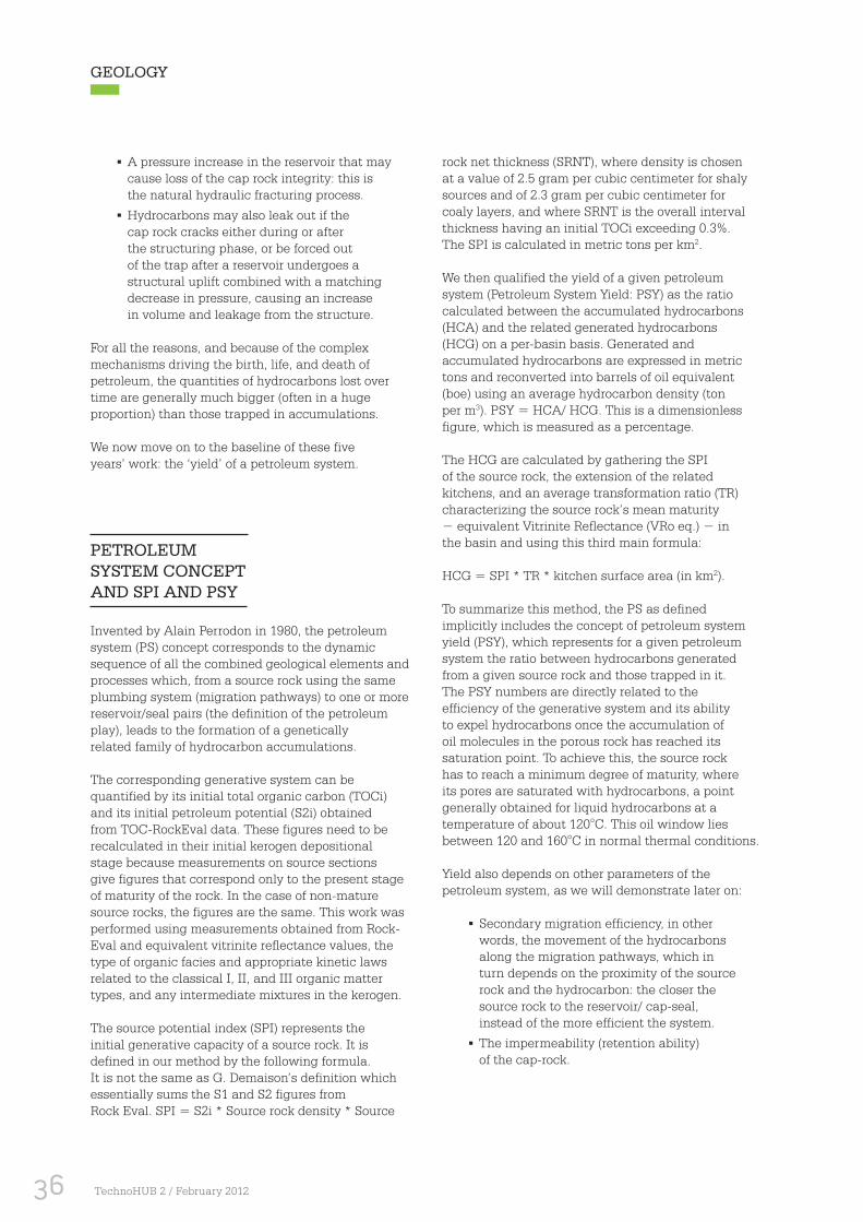
36 TechnoHUB 2 / February 2012
PETROLEUM SYSTEM CONCEPT AND SPI AND PSY
Invented by Alain Perrodon in 1980, the petroleum system (PS) concept corresponds to the dynamic sequence of all the combined geological elements and processes which, from a source rock using the same plumbing system (migration pathways) to one or more reservoir/seal pairs (the definition of the petroleum play), leads to the formation of a genetically related family of hydrocarbon accumulations.
The corresponding generative system can be quantified by its initial total organic carbon (TOCi) and its initial petroleum potential (S2i) obtained from TOC-RockEval data. These figures need to be recalculated in their initial kerogen depositional stage because measurements on source sections give figures that correspond only to the present stage of maturity of the rock. In the case of non-mature source rocks, the figures are the same. This work was performed using measurements obtained from Rock-Eval and equivalent vitrinite reflectance values, the type of organic facies and appropriate kinetic laws related to the classical I, II, and III organic matter types, and any intermediate mixtures in the kerogen.
The source potential index (SPI) represents the initial generative capacity of a source rock. It is defined in our method by the following formula. It is not the same as G. Demaison’s definition which essentially sums the S1 and S2 figures from Rock Eval. SPI = S2i * Source rock density * Source
rock net thickness (SRNT), where density is chosen at a value of 2.5 gram per cubic centimeter for shaly sources and of 2.3 gram per cubic centimeter for coaly layers, and where SRNT is the overall interval thickness having an initial TOCi exceeding 0.3%. The SPI is calculated in metric tons per km2.
We then qualified the yield of a given petroleum system (Petroleum System Yield: PSY) as the ratio calculated between the accumulated hydrocarbons (HCA) and the related generated hydrocarbons (HCG) on a per-basin basis. Generated and accumulated hydrocarbons are expressed in metric tons and reconverted into barrels of oil equivalent (boe) using an average hydrocarbon density (ton per m3). PSY = HCA/ HCG. This is a dimensionless figure, which is measured as a percentage.
The HCG are calculated by gathering the SPI of the source rock, the extension of the related kitchens, and an average transformation ratio (TR) characterizing the source rock’s mean maturity − equivalent Vitrinite Reflectance (VRo eq.) − in the basin and using this third main formula:
HCG = SPI * TR * kitchen surface area (in km2).
To summarize this method, the PS as defined implicitly includes the concept of petroleum system yield (PSY), which represents for a given petroleum system the ratio between hydrocarbons generated from a given source rock and those trapped in it. The PSY numbers are directly related to the efficiency of the generative system and its ability to expel hydrocarbons once the accumulation of oil molecules in the porous rock has reached its saturation point. To achieve this, the source rock has to reach a minimum degree of maturity, where its pores are saturated with hydrocarbons, a point generally obtained for liquid hydrocarbons at a temperature of about 120°C. This oil window lies between 120 and 160°C in normal thermal conditions.
Yield also depends on other parameters of the petroleum system, as we will demonstrate later on:
▪ Secondary migration efficiency, in other words, the movement of the hydrocarbons along the migration pathways, which in turn depends on the proximity of the source rock and the hydrocarbon: the closer the source rock to the reservoir/ cap-seal, instead of the more efficient the system.
▪ The impermeability (retention ability) of the cap-rock.
▪ A pressure increase in the reservoir that may cause loss of the cap rock integrity: this is the natural hydraulic fracturing process.
▪ Hydrocarbons may also leak out if the cap rock cracks either during or after the structuring phase, or be forced out of the trap after a reservoir undergoes a structural uplift combined with a matching decrease in pressure, causing an increase in volume and leakage from the structure.
For all the reasons, and because of the complex mechanisms driving the birth, life, and death of petroleum, the quantities of hydrocarbons lost over time are generally much bigger (often in a huge proportion) than those trapped in accumulations.
We now move on to the baseline of these five years’ work: the ‘yield’ of a petroleum system.
GEOLOGY

37February 2012 / TechnoHUB 2
Figure1: Relationship between SPI and age of the source rocks.
Uusually, Type II are transformed as maturity increases with burial depth, in a range of vitrinite reflectance of 0.6/0.7 and 1% and are termed ‘oil-prone’, i.e., inside the oil window. Type-III organic matter has much more delayed kinetics (only 30% of the organic matter is transformed at 1% VRo) and, chiefly for this reason, is considered as more gas-prone despite the fact that the Niger delta, for example, has delivered considerable amounts of liquids (oils and condensates).
Looking first at the statistics in Type II organic matter case studies and SPI variations over geological time, it is easy to recognize the importance of six main time stages (figure 1):
▪ Silurian, with its well-known hot shale radioactive layers, identified in North Africa and in the Arabian Platform, where intervals correspond to trangressive marine maximum flooding surface layers.
▪ Devonian and Frasnian/Famennian, also exhibiting typical radioactive hot-shale flooding layers, are well calibrated in North Africa and South America (shelf deposits).
▪ Kimmeridgian is a major contributor in the North Sea (Kimmeridge clay), in Western Siberia (Bazhenov formation), and in the South Aquitaine Basin (Lons or Lituolidae formations), but is absent as source rock facies in the southern flank of the Pyrenees in Spain.
WORLDWIDE SPI STATISTICS
Generally, as G. Demaison has done, we can define and rank SPI figures which are less than 2.5 million metric tons per km2 (a threshold that represents a risk of associated hydrocarbon undercharge) as low. Values between 2.5 and 7.5 million metric tons per km2 are considered as moderate (normal hydrocarbon charge), while SPI ranging between 7 and 15 million metric tons per km2 are classified as high (also recognized as hydrocarbon supercharge).
We compiled SPI statistics, differentiating Type II kerogens (mainly algal marine organic matter) from Type III kerogens (composed of continental humic materials, generally related to deltas or substantial fluvial fairways with a large influx of sediments originating from the continent).
Generally speaking, PSYs are clearly fairly low, at just a few percent. This is because losses occur throughout the system, first of all in the source rock, then along the migration pathways, and finally in the petroleum trap. Our study incorporates extensive in-house statistics on SPI and calculations of PSY which illustrate in the rest of this paper.
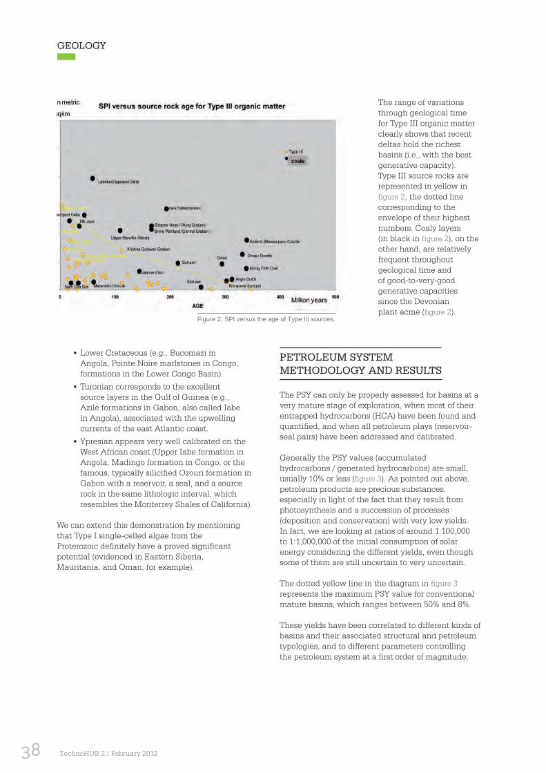
38 TechnoHUB 2 / February 2012
▪ Lower Cretaceous (e.g., Bucomazi in Angola, Pointe Noire marlstones in Congo, formations in the Lower Congo Basin).
▪ Turonian corresponds to the excellent source layers in the Gulf of Guinea (e.g., Azile formations in Gabon, also called Iabe in Angola), associated with the upwelling currents of the east Atlantic coast.
▪ Ypresian appears very well calibrated on the West African coast (Upper Iabe formation in Angola, Madingo formation in Congo, or the famous, typically silicified Ozouri formation in Gabon with a reservoir, a seal, and a source rock in the same lithologic interval, which resembles the Monterrey Shales of California).
We can extend this demonstration by mentioning that Type I single-celled algae from the Proterozoic definitely have a proved significant potential (evidenced in Eastern Siberia, Mauritania, and Oman, for example).
PETROLEUM SYSTEM METHODOLOGY AND RESULTS
The PSY can only be properly assessed for basins at a very mature stage of exploration, when most of their entrapped hydrocarbons (HCA) have been found and quantified, and when all petroleum plays (reservoir-seal pairs) have been addressed and calibrated.
Generally the PSY values (accumulated hydrocarbons / generated hydrocarbons) are small, usually 10% or less (figure 3). As pointed out above, petroleum products are precious substances, especially in light of the fact that they result from photosynthesis and a succession of processes (deposition and conservation) with very low yields. In fact, we are looking at ratios of around 1:100,000 to 1:1,000,000 of the initial consumption of solar energy considering the different yields, even though some of them are still uncertain to very uncertain.
The dotted yellow line in the diagram in figure 3 represents the maximum PSY value for conventional mature basins, which ranges between 50% and 8%.
These yields have been correlated to different kinds of basins and their associated structural and petroleum typologies, and to different parameters controlling the petroleum system at a first order of magnitude:
The range of variations through geological time for Type III organic matter clearly shows that recent deltas hold the richest basins (i.e., with the best generative capacity). Type III source rocks are represented in yellow in figure 2, the dotted line corresponding to the envelope of their highest numbers. Coaly layers (in black in figure 2), on the other hand, are relatively frequent throughout geological time and of good-to-very-good generative capacities since the Devonian plant acme (figure 2).
GEOLOGY
Figure 2: SPI versus the age of Type III sources.

39February 2012 / TechnoHUB 2
▪ Tectonic and sedimentary histories, type of structural settings and relationships between the main components of the petroleum system: source rock, reservoir and seal as well as their deposition dynamics.
▪ Hydrocarbon migration distances (long or short distances between the source rocks and the petroleum plays).
This basin classification has been used by simple type-analogy as a tool for estimating both the maximum value of the ultimate petroleum potential and the quantities remaining to be discovered in either a whole basin or in less explored parts of a basin (YTF volumes). This YTF figure, recognized as a possible maximum value, is calculated by evaluating the hydrocarbons generated for all proved or speculative sources of the basin and multiplying by a chosen PSY corresponding to the Basin type. The resulting value can be usefully compared in our statistics to other approaches, such as the mode figures, obtained by summing the notional volumetrics of speculative petroleum plays, leads, and prospects (analytical phase). It corresponds to the maximum threshold, suggesting that new petroleum plays and prospects may yet be found.
It also helps tentatively to assess unconventional hydrocarbon resources which have to be added to conventional fields and prospects and notional conventional plays already identified. The efficiency of the petroleum systems was calibrated, in our study, on 70 basins of different typologies considered as mature-to-very-mature in terms of exploration degree and having a satisfying distribution of quantified source rock parameters.
The appropriate PSY values were applied to a total of 175 selected basins studied primarily to calculate YTF figures. Sensitivity tests (experimental design studies) carried out on SPI and PSY figures have clearly shown them to be essentially contingent on three major uncertainties:
Figure 3: Worldwide basin study (note that the three red squares plotted above the yellow line represent unconventional resources calculated for Venezuelan and Canadian Basins).
▪ Source rock extension and kitchen delineation
▪ Mean organic content, normally well calibrated in mature basins
▪ Source rock net thicknesses
The last of the above has generally been the most critical and most uncertain of the three parameters; even seismic data can be used to calculate the gross thickness of the source section but not, of course, its net thickness (TOC > 0.3%). The PSY figures show a wide distribution, ranging between 0.1% and 50% (see figure 3).
We should bear in mind that the efficiency of a PS as defined above should not be confused with the hydrocarbon charge at drainage area scale (field or prospect) representing 10% to 60% yield figures.
Several parameters seem to control the distribution of the PSY figures:
▪ Size of the basin
▪ Typology, e.g., graben, passive margin, foothills
▪ Burial history
▪ Initial petroleum potential of the source layers (but not always)
▪ Degree of source rock maturity
▪ Migration type and distance
▪ Consistency or inconsistency between the structuring age and the timing of the hydrocarbon migration from the kitchen

40 TechnoHUB 2 / February 2012
Figure 5: Relationship between PSY and age of the source rocks.
A PSY scale was generated during the study (figure 4) in relation to the basin’s tectono-sedimentary contexts, ranking top PSY numbers for compact systems (those having a short hydrocarbon migration distance), decreasing through grabens and rifts, then foldbelts and salt gravity-driven basins, intra-cratonic basins and salt basins, followed by deltaic provinces, and lastly basins with old source rocks or low migration-timing coherency.
The most efficient sedimentary basins are associated with compact systems, where proximity between the source rock and the petroleum plays (reservoir and associated seal) is excellent. The optimal geometry is considered to occur when there is full imbrication between the organic facies and the reservoirs, for example in penesaline environments (Oman stringers) or in turbidite environments.
GEOLOGY
Figure 4: Basin types and order of magnitude of the PSY fi gure/basin type scale.

41February 2012 / TechnoHUB 2
The Gabonese Senonian Basin is a very good example of this kind of setting with its imbricated generally silicified (diatomites) source and reservoir intervals associated with early kinetic behaviours favoured by a lipidic protopetroleum presence. Especially good examples are when the source interval plays a sealing role (allowing a per descensum/per laterum hydrocarbon migration process), e.g., Silurian hot shales in North Africa or example of the Kimmeridge Clay in the North Sea.
The least efficient systems are observed in ancient deposits (Paleozoic and Proterozoic) where the complexity of the structural history, the long duration of an uncertain but compulsory retention, and the occurrence of structural inversions can lead to changes of hydrocarbon phase and possible leakages associated with seal breaching (figure 5). The presence of evaporites as cap- rocks helps to preserve traps from leakages.
Deltas have low PS efficiency, probably due to the significant dilution of the source layers composed mainly of poor humic continental organic matter, often distributed in thick intervals, and due also to the dispersion of hydrocarbons migrating in several multi-layered reservoirs, defining a complex plumbing system. The study has demonstrated that the source rock age (figure 5) and the lateral migration distance (figure 6) are other key factors in controlling the PSY. In figure 6, the basins within the dotted green ellipse are those whose main process is controlled more by vertical than lateral migration.
Figure 6: Relationship between PSY and lateral migration distance.

42 TechnoHUB 2 / February 2012
Figure 7: Example of the South Aquitaine Basin, France. Stratigraphic chart in Biteau et al., 2006.
GEOLOGY

43February 2012 / TechnoHUB 2
Figure 8: Example of differentiated typologies and related PSY.
TWO CASE STUDIES
We will now illustrate these assessments with two examples extracted from the database built during our study: the Aquitaine basin (Biteau et al., 2006) and a compilation of some African Basins located in North and Sub-Saharan areas.
AQUITAINE BASIN
Despite the low SPI of its main generative system (of the order of 1 million metric tons per km2), the South Aquitaine Basin offers a fine example of a really efficient compact system (PSY=12%), exhibiting a short distance between source and plays, i.e., Kimmeridgian source and Barremian-Tithonian−Kimmeridgian reservoirs, associated with a foreland area and a main vertically-driven hydrocarbon migration process.
AFRICAN BASINS
Typological differences and associated yields are also well evidenced by the comparison of some of the West and North Africa basins, see figure 8.
DISCUSSION ON YTF FIGURES
It is typically in the framework of a worldwide YTF hydrocarbon evaluation project (inventory and ranking of remaining hydrocarbon volumes) that our PSY method has been put into practice since 2005. It enabled us to calculate the maximum remaining exploration potential of some underexplored basins on which we cannot comment in detail here.
We will present here the main conclusions from this study and describe two case studies to illustrate our comments and indeed highlight the principal advantage of this method.
The most striking results concern the offshore extension of well-calibrated onshore basins such as the Sirt Basin in Libya or others with a clearly differentiated exploration history, for example in Brazil and Australia. For the other basins, the choice of a pertinent geological and petroleum analogue is the most crucial criterion in their PSY selection.
In poorly calibrated frontier areas, the method remains sensitive to the lack of identified source rocks, poor SPI knowledge, and source maturity uncertainties. In these contexts, it is more challenging to correctly calculate the generated volumes. Core drills and outcrop sampling have proved to be very useful references and have further enhanced our evaluations. For example, we were able to identify the East Greenland Basin as one of the anomalies (possible remaining exploration potential) in line with a recently published USGS document (USGS, 2000).
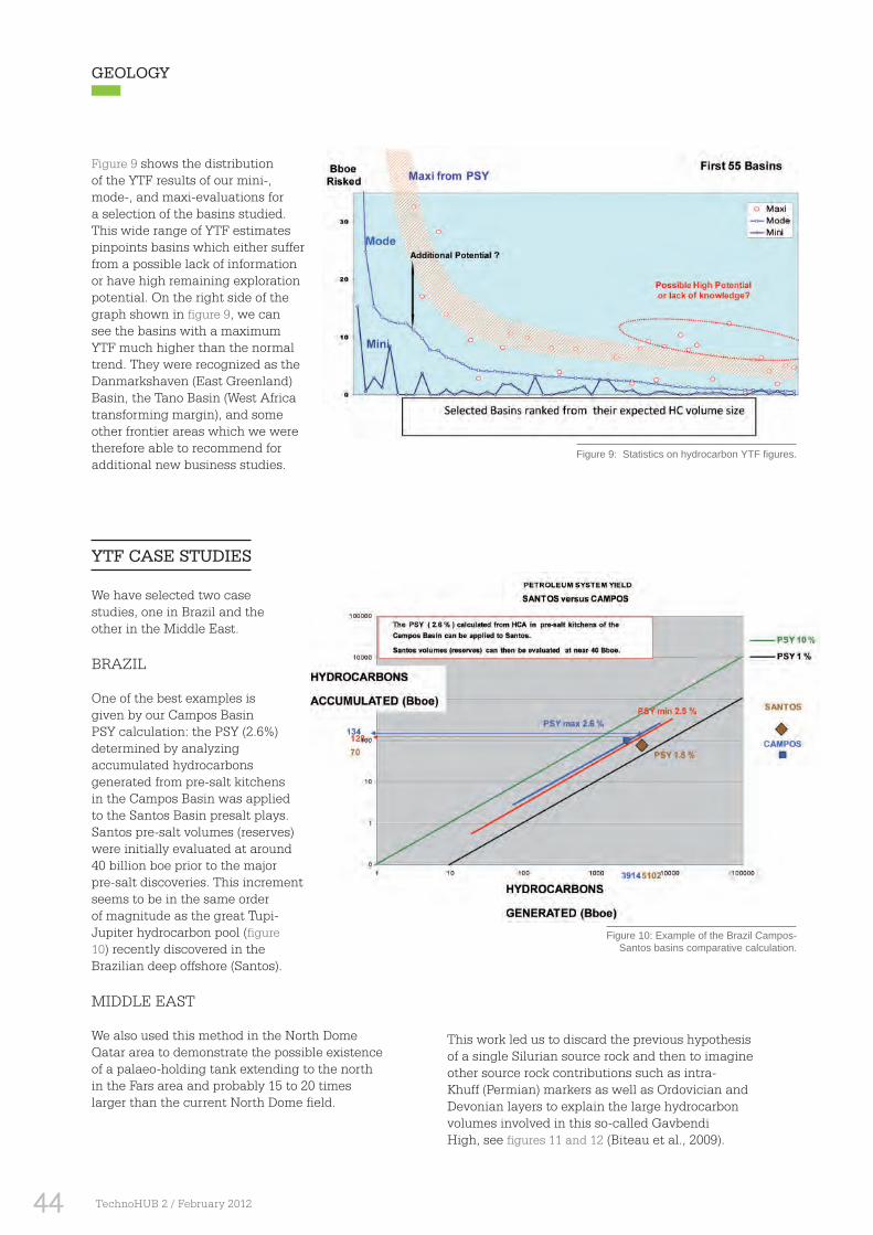
44 TechnoHUB 2 / February 2012
YTF CASE STUDIES
We have selected two case studies, one in Brazil and the other in the Middle East.
BRAZIL
One of the best examples is given by our Campos Basin PSY calculation: the PSY (2.6%) determined by analyzing accumulated hydrocarbons generated from pre-salt kitchens in the Campos Basin was applied to the Santos Basin presalt plays. Santos pre-salt volumes (reserves) were initially evaluated at around 40 billion boe prior to the major pre-salt discoveries. This increment seems to be in the same order of magnitude as the great Tupi-Jupiter hydrocarbon pool (figure 10) recently discovered in the Brazilian deep offshore (Santos).
MIDDLE EAST
We also used this method in the North Dome Qatar area to demonstrate the possible existence of a palaeo-holding tank extending to the north in the Fars area and probably 15 to 20 times larger than the current North Dome field.
Figure 9 shows the distribution of the YTF results of our mini-, mode-, and maxi-evaluations for a selection of the basins studied. This wide range of YTF estimates pinpoints basins which either suffer from a possible lack of information or have high remaining exploration potential. On the right side of the graph shown in figure 9, we can see the basins with a maximum YTF much higher than the normal trend. They were recognized as the Danmarkshaven (East Greenland) Basin, the Tano Basin (West Africa transforming margin), and some other frontier areas which we were therefore able to recommend for additional new business studies.
Figure 9: Statistics on hydrocarbon YTF fi gures.
Figure 10: Example of the Brazil Campos-Santos basins comparative calculation.
This work led us to discard the previous hypothesis of a single Silurian source rock and then to imagine other source rock contributions such as intra-Khuff (Permian) markers as well as Ordovician and Devonian layers to explain the large hydrocarbon volumes involved in this so-called Gavbendi High, see figures 11 and 12 (Biteau et al., 2009).
GEOLOGY

45February 2012 / TechnoHUB 2
Figure 11: The Gavbendi High hydrocarbon dysmigration and remobilization concept (Biteau et al., 2009b).
Figure 12: Quantitative approach: how to discard a single source rock concept (Biteau et al., 2009).
REFERENCES
Andreini et al. [2008] Understanding the future, Geosciences serving society. Nancy School of Geology, Editions Hirle.
Biteau, J.J., Perrodon, A. and Choppin de Janvry G. [2003] The Petroleum System: a fundamental tool. Oil and Gas Journal, 11 August.
Biteau J.J., Le Marrec, A. Le Vot, M. and Masset, J.M. [2006] The Aquitaine Basin. Petroleum Geoscience, 12(3), 247-273.
Biteau et al. [2007] The Petroleum System, a global quantitative approach at Basin and fi eld scales, which lessons for some of the Lower Congo Basin Petroleum systems. DOWAC, Luanda.
Biteau et al. [2008] African Petroleum Systems: richness and effi ciency key drivers at continent scale. AAPG, Cape Town.
Biteau et al. [2009a] The Gulf of Guinea Petroleum Systems, pre-salt and post-salt dichotomy. AAPG, Rio de Janeiro.
Biteau et al. [2009b The Khuff play related Petroleum System between the Qatar arch and the Fars area. IPTC, Doha.
Demaison, G. [1984] The generative basin concept. In Demaison, G.and Murris, R.J., (Eds) Petroleum geochemistry and basin evaluation. AAPG Memoir, 35, 1–14.
Dow, W.G. [1974] Application of oil correlation and source rock data to exploration in Williston basin. AAPG Bulletin, 58, 7, 1253−1262.
Klemme, H.D. [1994] Petroleum Systems in the world that involve Upper Jurassic source rocks. AAPG Memoir, 60, 51−72.
Magoon, L.B. [1988] The Petroleum System – A classifi cation scheme for research, resource assessment. USGS Bulletin, 1870, 2−15.
Magoon, L.B. and Dow, W.G. [1994] The Petroleum System. AAPG Memoir, 60, 3−23.
Magoon L.B. and Valin Z.C. [1994] Overview of Petroleum System case studies. AAPG Memoir, 60, 329−338.
Magoon L.B. et al. [2002] Petroleum Systems of the Alaskan North Slope – a progress report. AAPG Bulletin, 6, 86, 1151 (Abstract).
Perrodon A. [1992] Petroleum systems, models and applications. Journal of Petroleum Geology, 15(3), 319−326.
USGS [2000] World Petroleum assessment 2000 – Description and Results. USGS Digital Data Series, 60.

46 TechnoHUB 2 / February 2012
In exploration and production, the quality of geological interpretation is key to assessing exploration potential, evaluating hydrocarbon discoveries and ultimately optimizing their production.
Rock cores cut from wellbores provide key information and allow geological interpretation for reservoir extension. Using new tools and innovative methods of interpreting borehole images, a significant part of this information can now be obtained on uncored reservoirs as well, thanks to the tremendous improvements in the image resolution and quality of image logs, achieved over the last fifteen years.
The method for interpreting the log images begins by calibrating the images of available cored intervals. This is followed by interpreting the uncored sections. The final step entails integration into the 3D geological context using the seismic data and sedimentological knowledge. Interpretation consists in classifying the borehole images and associating them with sedimentary deposits, called sedimentary facies. These elements are then used to reconstruct the context in which the sediments were deposited.
This paper summarizes the imaging interpretation experience acquired by Total in the area of deepwater turbidite sediments. The analogies between the features observed on image logs and those seen on cores and surface rock outcrops are clearly illustrated. It is now possible to obtain good-quality image recognition and interpretation without core calibration, even for the first exploration well of a discovery, in a well-known geological context.
The technique is being extended to all types of sedimentary environment (fluviatile, lacustrine, deltaic, glacial). It can be applied in the context of exploration wells to facilitate the initial diagnosis of sedimentary environments. It is also widely used in the context of appraisal and development wells, where the results of detailed interpretation can be integrated quickly and successfully into the process of field evaluation and reserves estimation.
Since image logs can yield valuable and high-quality geological interpretation results, it can be decided to acquire image logs rather than cores in certain defined domains. The advantage is that image logs provide many more data both at well scale (since they can be logged over longer sections than coring operations and at much lower cost) and at field scale, with multi-well acquisitions. This therefore allows a substantial reduction in coring costs without diminishing sedimentological understanding. However, cores will still be necessary for petrophysical analysis and sedimentological calibration in unknown contexts.
The main advantages of developing this specialty in-house at Total are thus twofold: enhancing the quality of geological evaluation within the field evaluation process, while optimizing data acquisition costs. The fact that this paper received the Eötvös Award at EAGE Vienna 2011 confirms the interest of the approach.
GEOLOGY
CONTEXT

47February 2012 / TechnoHUB 2
Borehole image logs for turbidite facies identification: core calibration and outcrop analogues
In exploration, appraisal, and development of hydrocarbon fields, the understanding of the sedimentary model requires increasingly sophisticated techniques and analysis to interpret the geometry, facies, and petrophysical properties of the reservoirs. The objective is to understand the reservoir flow properties for making optimum decisions during field development. For this purpose, the use of high resolution image logs provided by service companies has become essential in sedimentary interpretation. When they are correctly calibrated against known facies, image logs can replace coring operations, which are time-consuming, expensive, and limited in the depth interval sampled. Recent examples of application have proved highly successful for exploration wells.
Now mature fields can be reinterpreted in the light of the new understanding gained, enabling development plans to be revised with enhanced recovery methods. As a result of the success of this approach, imagebased facies interpretation is now included in the standard procedure for evaluation of data from exploration, appraisal, and development wells.
Jean-Bernard JOUBERT1* and Valérie MAÏTAN1
1 Total Technical Centre, Avenue Larribau, 64018 Pau, France.*Corresponding author, E-Mail: [email protected]
EXTRACTFirst BreakVol 28Issue 6June 2010
ABSTRACT

48 TechnoHUB 2 / February 2012
Figure 1: Work fl ow of an image logs study showing integration of these data (facies and dips) in the sedimentary model. Each sedimentary body will be ascribed petrophysical properties in the reservoir model for oil volume calculation.
INTRODUCTION
In recent years, the need for improved reservoir knowledge from deep exploration wells has become acute because of the general requirement for fast-track discovery evaluation coupled with the lack of nearby outcrops of reservoir rocks. In addition, the high heterogeneity of turbidite reservoirs poses special problems for reserves estimation and fluid-flow prediction. Since starting exploration in deepwater areas offshore Africa in the 1990s, Total has carried out intense coring acquisition programmes in more than 20 turbidite oil fields. Coring remains the best reservoir calibration reference, because the mineralogical and petrophysical characteristics of the sediments can be determined unambiguously from core. During the same period, image logging in oilbased mud has become possible, albeit providing images of lower resolution. This technological development has made it possible to interpret facies in detail over the complete drilled section in many more wells.
In the absence of core, borehole image logging is the fastest and most precise method for extracting the data needed for spatial extrapolation to build the sedimentary model. Because less coring is required when imaging logs are run, there are large cost saving in field development. The accuracy of
image log interpretation is strongly influenced by the initial quality of data, which means tight quality control is mandatory. To avoid mis-interpretation and over-interpretation, the following checks need to be made before starting to interpret the data:
▪ Logging condition and orientation of the tool in borehole
▪ Proper functioning of the imaging instrument (sensors, navigation system)
▪ Calculation of the exact position of each pixel on the cylinder representing the borehole surface (speed correction)
▪ Estimation of the depth of investigation of the sensors
▪ Optimal choice of the false-colour scale used to image the physical variable
▪ Recognition of artifacts arising from the measurement system and data processing
Coupled with compositional information from petrophysical logs, high resolution borehole images provide sedimentary facies description at a level of detail and accuracy which is close to that obtained from core and outcrop observations. The results can be integrated into a 3D gridded sedimentary model, as illustrated in figure 1.
GEOLOGY

49February 2012 / TechnoHUB 2
SEDIMENTARY FACIES FROM IMAGE LOGS
The requirement is to predict sedimentary facies over the complete section of a well. Our methodology is to define the image sedimentary facies (ISF) in a procedure which integrates image characteristics with sedimentological concepts. An ISF corresponds to a specific lithology and depositional mechanism within a given sedimentary environment.
A first lithological determination is provided by a classical multi cut-off method based on a quantitative estimate of the clay content, sonic and density log responses, and the separation of neutron and density logs. This determination is mainly, but not only, dependent on the sand/shale content of the formation, and is made without regional bias. Then it is refined using a neural network computation based on the log responses from different tools. The limitations on identification of facies from such lithology determination arises from possible confusion between formation with similar sand/shale ratios, such as a basal lag with large shaly clasts and a sand-rich debris flow, and the limited resolution of these logs, which do not provide any sedimentological information of the penetrated strata.
Additional information, such as bed thickness and the nature of bed contacts, is obtained by visual analysis of the texture of the images in order to identify the ISF. This information includes the categorization of imaged surfaces and measurement of their dip azimuths. It is combined with the geological information obtained at the well site on lithology, grain size, and cement, and the compositional data available from the interpretation of petrophysical logs. The ISF is more than a wireline neural network-based facies because it is calibrated as closely as possible to the regional sedimentological macrofacies.
A calibration plate has been designed to define each facies to limit the risk of subjective bias by an interpreter. It summarizes all information concerning the facies and includes an example of its appearance for each basic type of imaging tool – electrical resistivity in oil-based mud, electrical conductivity in water-based mud, and acoustic reflectivity in both types of mud. Of course, we do not have all the image types from the same well, so the examples have to be composed from several wells or fields. Figure 2 displays part of the ISF calibration plate defining debris flow facies in a deep marine environment. At least one image in a calibration plate corresponds to the logs and to the cores shown, but the other types of image are also calibrated on cores.
Figure 2: Description and calibration sheet for the debris fl ow facies, with recognition of typical structures, and depositional or deformation interpretations on wireline logs, cores, and image logs. The formations appear in yellow if resistive (oil-bearing sandstone), and brown if conductive (clays/water-saturated sandstone).

50 TechnoHUB 2 / February 2012
The image contrast for electrical imager tools is referred to as ‘relative conductivity’, as obtained from imagers that operate in water-based mud such as Schlumberger’s FMI tool. Conductivity is largely determined by fluids, so high values are found in brine-saturated or shaly intervals and low values are found in hydrocarbon-saturated or cemented intervals. Increasing conductivity is represented as increasing colour saturation, from white to brown.
The low resolution and coverage of imaging tools for use in oil-based muds makes their interpretation much more difficult than for images obtained from tools used in waterbased muds. Long experience and good understanding of drill-site operations, sedimentology, and the physics of acquisition is therefore required to avoid misinterpretation.
DEFINITION OF IMAGE SEDIMENTARY FACIES
High resolution borehole image logs provide a sedimentary facies close to that obtained from core and outcrop observations. The ISF is calibrated as closely as possible to the definition
of the corresponding regional sedimentological macrofacies. Each ISF is defined by specific invariant characteristic, stable for all interpreters and valid for all countries and all wells. Consequently, the risk bias due to subjective judgement of the interpreter is limited.
The descriptions of facies in this paper use Total’s in-house facies nomenclature for turbidite environments. The main types of sedimentary facies are: hemipelagites to massive shale, mud turbidites to laminated shale, thin-bedded turbidites, low density turbidites, high density turbidites, and debris flows. Certain post-depositional features are also recognizable: slumps, sandy injections, and cementation/diagenesis.
Eleven ISFs have been defined for borehole image interpretation in a deepwater offshore sedimentary environment. The nomenclature and classification are illustrated in figure 3 and are given in this section. The ISFs were identified in hydrocarbon fields in the Gulf of Guinea. Figures 4 to 12 display, by ISF type, examples of image logs compared with core and outcrop. Images and cores are not presented at the same scale but are within the same interval. The image logs are speedcorrected and oriented ‘North to North’.
Figure 3: Image sedimentary facies (ISF) scheme.
GEOLOGY

51February 2012 / TechnoHUB 2
ISF 1: MASSIVE SHALE
This facies is deposited as mud settling from suspension. On wireline logs, it is detected through conventional shale indicators (high clay content, large neutron/density separation, and low velocity). The image is mainly conductive, and very thinly laminated (figure 4). These shales are finely foliated and dips are picked with a low accuracy. Some unreliable, thin, resistive stringers or halos, due to bioturbation or diagenetic nodules, cut across the image. This ISF is well discriminated by conventional logs and constitutes a good seal.
ISF 2: MUD TURBIDITES TO LAMINATED SHALE
This facies is described on cores as a shaly formation with occasional silty beds or laminae with current ripples. On conventional logs, these shaly facies are discriminated by sonic and neutron/density separation. The image shows a dominant conductive pattern (brown to orange) with thin resistive layers visible on all pads (figure 5). The dips are fairly accurately picked. This is not a reservoir facies.
Mud turbidites are often mistaken from mud-rich debris flows because both facies display low resistivity images, and large elongated clasts within debris flows can be confused with laminations on the image. In addition, dewatering processes within mud turbidite or heterolithic intervals may appear similar to debris flow deposits on image logs.
ISF 3: LOW-DENSITY GRAVITY FLOW DEPOSITS – HETEROLITHIC, SHALE DOMINANT
This facies corresponds to centimetre-scale, silty to fine sand and shale sequences, with shale dominating. On conventional logs, the facies appears as variably argillaceous silts. The image shows dominant brown continuous beds and resistive white concordant bed contacts (figure 6 p. 52). Dips are homogeneous with plane-parallel bedding. Locally contorted contacts may cause confusion of this facies with thin debris flows or conglomerates. This facies has poor reservoir characteristics. The net sand-shale ratio is estimated to be rather low according to conventional wireline logs, quantitative interpretation, and regional core calibration.
Figure 4: ISF 1 - massive shale.
Figure 5: ISF 2 - mud turbidites to laminated shale.

52 TechnoHUB 2 / February 2012
ISF 4: LOW- DENSITY GRAVITY FLOW DEPOSITS – HETEROLITHIC, SAND DOMINANT
This heterolithic facies is composed of decimetre-scale alternations of very fine to fine sand and shale, but with sand being dominant. On conventional logs, this facies appears as shaly sand to silt. Image logs show decimetre-scale conformable alternations of dominantly resistive continuous sandy beds (white–yellow) and shale (brown) (figure 7). The bedding is plane-parallel with locally slight erosion at base (Bouma sequences). The acronym LRS, standing for low resistivity sand, is reserved for hydrocarbon-bearing lowdensity turbidites that are fairly rich in sand. They are distinguished from unconformable sands such as injections or sandy debris flows. The net sand ratio of this facies is about 50%, judging from conventional wireline logs, quantitative interpretation, and regional core calibration.
ISF 5 AND ISF 6: SANDY HIGH- DENSITY FLOW DEPOSITS – MASSIVE/LAMINATED FINE TO GRAVELLY SANDS
These metre-scale massive to laminated clean sand facies correspond to fine/medium-grained sands and poorly sorted coarse-grained sands, respectively. They are clearly identifiable on wireline logs. The image (figure 8) shows dominantly resistive hydrocarbon-bearing beds (left image). A dynamic normalization focused on the reservoir interval shows massive sands, laminated sands, and fairly chaotic events associated with very small-scale dip variations within individual sand beds (right image, with contrast enhancement). Current imaging techniques do not allow for an interpretation of the image in terms of sand grain size. The grain size is provided by cuttings or sidewall cores, when available. These facies are restricted to clean sand responses on wireline logs and resistive images. Therefore, the net-togross sand ratio is high. The best reservoir characteristics are ascribed to ISF 5.
Figure 6: ISF 3 - low-density gravity fl ow deposits – heterolithic, shale dominant.
Figure 7: ISF 4 - low-density gravity fl ow deposits – heterolithic, sand dominant.
ISF 7 AND ISF 8: MUD-RICH TO SAND-RICH DEBRIS FLOWS
In these ISFs, silty-sandy and argillaceous components are typically distinguished by the proportion of grains floating in the argillaceous matrix (figure 9). In ISF 7, floating elements represent less than 20% of the volume. ISF 8 is similar but siltier/sandier, and has up to 40% floating elements. Large clasts may also be present. No consistent pattern is apparent on conventional logs: they appear as shaly or silty. Dips are difficult to identify. Images in this formation are highly heterogeneous and ‘lumpy’. Discrimination between the mud-rich and sand-rich facies is achieved by using conventional log cut-offs and image colouring. These ISFs lack any of the characteristics required for a good reservoir. To distinguish between a mass-flow deposit associated with turbiditic flow in a channel and a mass transport complex due to a slide with an associated headwall scar, seismic data must be used.
GEOLOGY
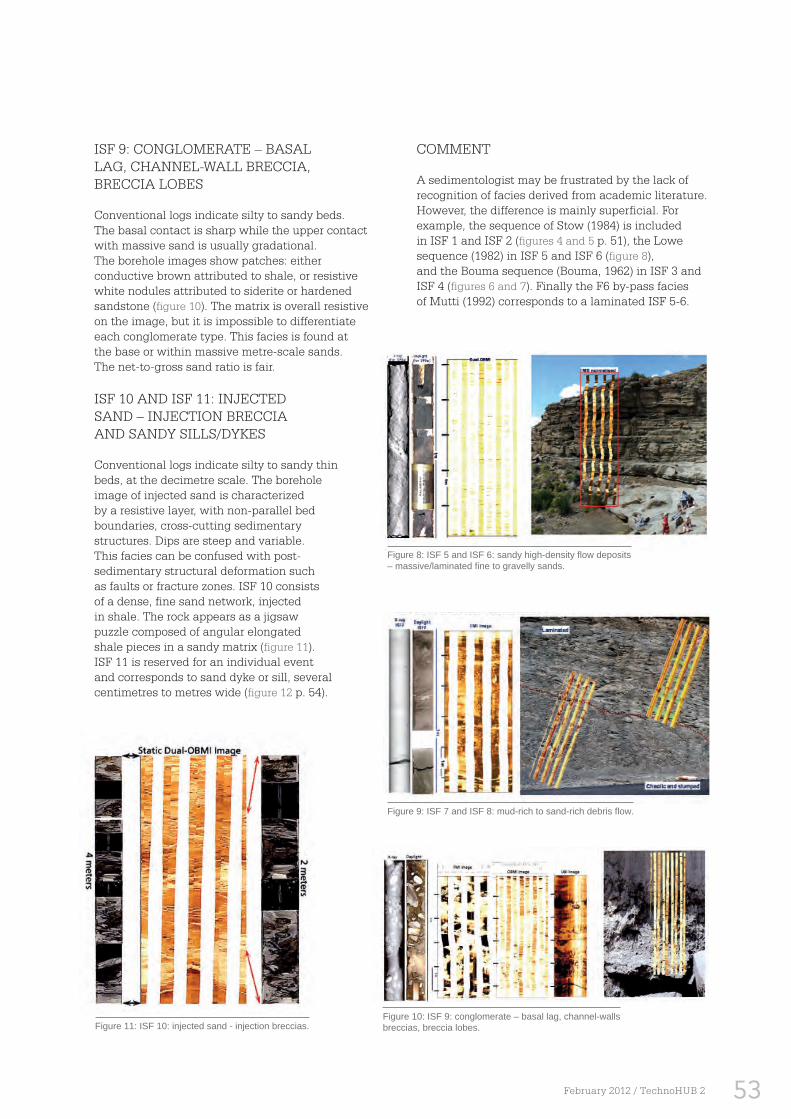
53February 2012 / TechnoHUB 2
Figure 8: ISF 5 and ISF 6: sandy high-density fl ow deposits – massive/laminated fi ne to gravelly sands.
Figure 10: ISF 9: conglomerate – basal lag, channel-walls breccias, breccia lobes.
ISF 9: CONGLOMERATE – BASAL LAG, CHANNEL-WALL BRECCIA, BRECCIA LOBES
Conventional logs indicate silty to sandy beds. The basal contact is sharp while the upper contact with massive sand is usually gradational. The borehole images show patches: either conductive brown attributed to shale, or resistive white nodules attributed to siderite or hardened sandstone (figure 10). The matrix is overall resistive on the image, but it is impossible to differentiate each conglomerate type. This facies is found at the base or within massive metre-scale sands. The net-to-gross sand ratio is fair.
ISF 10 AND ISF 11: INJECTED SAND – INJECTION BRECCIA AND SANDY SILLS/DYKES
Conventional logs indicate silty to sandy thin beds, at the decimetre scale. The borehole image of injected sand is characterized by a resistive layer, with non-parallel bed boundaries, cross-cutting sedimentary structures. Dips are steep and variable. This facies can be confused with post-sedimentary structural deformation such as faults or fracture zones. ISF 10 consists of a dense, fine sand network, injected in shale. The rock appears as a jigsaw puzzle composed of angular elongated shale pieces in a sandy matrix (figure 11). ISF 11 is reserved for an individual event and corresponds to sand dyke or sill, several centimetres to metres wide (figure 12 p. 54).
COMMENT
A sedimentologist may be frustrated by the lack of recognition of facies derived from academic literature. However, the difference is mainly superficial. For example, the sequence of Stow (1984) is included in ISF 1 and ISF 2 (figures 4 and 5 p. 51), the Lowe sequence (1982) in ISF 5 and ISF 6 (figure 8), and the Bouma sequence (Bouma, 1962) in ISF 3 and ISF 4 (figures 6 and 7). Finally the F6 by-pass facies of Mutti (1992) corresponds to a laminated ISF 5-6.
Figure 9: ISF 7 and ISF 8: mud-rich to sand-rich debris fl ow.
Figure 11: ISF 10: injected sand - injection breccias.
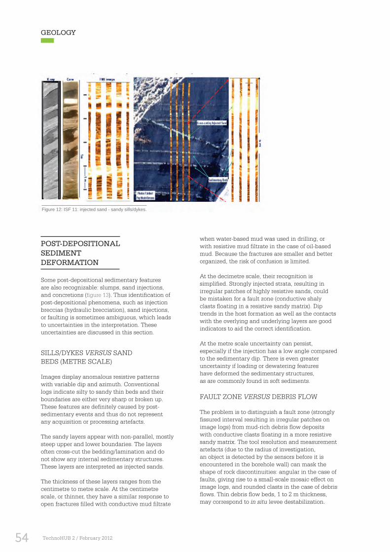
54 TechnoHUB 2 / February 2012
POST-DEPOSITIONAL SEDIMENT DEFORMATION
Some post-depositional sedimentary features are also recognizable: slumps, sand injections, and concretions (figure 13). Thus identification of post-depositional phenomena, such as injection breccias (hydraulic brecciation), sand injections, or faulting is sometimes ambiguous, which leads to uncertainties in the interpretation. These uncertainties are discussed in this section.
SILLS/DYKES VERSUS SAND BEDS (METRE SCALE)
Images display anomalous resistive patterns with variable dip and azimuth. Conventional logs indicate silty to sandy thin beds and their boundaries are either very sharp or broken up. These features are definitely caused by post-sedimentary events and thus do not represent any acquisition or processing artefacts.
The sandy layers appear with non-parallel, mostly steep upper and lower boundaries. The layers often cross-cut the bedding/lamination and do not show any internal sedimentary structures. These layers are interpreted as injected sands.
The thickness of these layers ranges from the centimetre to metre scale. At the centimetre scale, or thinner, they have a similar response to open fractures filled with conductive mud filtrate
when water-based mud was used in drilling, or with resistive mud filtrate in the case of oil-based mud. Because the fractures are smaller and better organized, the risk of confusion is limited.
At the decimetre scale, their recognition is simplified. Strongly injected strata, resulting in irregular patches of highly resistive sands, could be mistaken for a fault zone (conductive shaly clasts floating in a resistive sandy matrix). Dip trends in the host formation as well as the contacts with the overlying and underlying layers are good indicators to aid the correct identification.
At the metre scale uncertainty can persist, especially if the injection has a low angle compared to the sedimentary dip. There is even greater uncertainty if loading or dewatering features have deformed the sedimentary structures, as are commonly found in soft sediments.
FAULT ZONE VERSUS DEBRIS FLOW
The problem is to distinguish a fault zone (strongly fissured interval resulting in irregular patches on image logs) from mud-rich debris flow deposits with conductive clasts floating in a more resistive sandy matrix. The tool resolution and measurement artefacts (due to the radius of investigation, an object is detected by the sensors before it is encountered in the borehole wall) can mask the shape of rock discontinuities: angular in the case of faults, giving rise to a small-scale mosaic effect on image logs, and rounded clasts in the case of debris flows. Thin debris flow beds, 1 to 2 m thickness, may correspond to in situ levee destabilization.
Figure 12: ISF 11: injected sand - sandy sills/dykes.
GEOLOGY

55February 2012 / TechnoHUB 2
BENEFITS OF ISF CLASSIFICATION
As the ISFs are calibrated on cores and wireline logs, and correlated to outcrop analogues, the study of image logs is the best link from well data to seismic data. The integration of several independent data sources gives confidence in the interpretation, but for a good quality study, it is essential that the interpreter should apply the following rules:
1. Grain size estimation is provided by conventional geological techniques, such as cuttings descriptions, calcimetry, sidewall cores, and cores.
2. Lithology is the first guide to facies and is provided by neural- network computation from wireline logs. The lithology determination is representative of the sand/shale content of the formation.
3. Image log interpretation provides structural and textural information about the formation. This information complements the determination of lithology from logs within a range of sand/shale ratio. The only way of discriminating a sand-rich heterolithic deposit from a sand-rich debris flow is the texture: laminated for heterolithic and chaotic for debris flow.
This approach permits the integration of the various turbidite nomenclatures and can be applied to exploration wells or mature fields. Each ISF is defined by specific characteristics that are stable for all interpreters and valid for all countries and all wells. Consequently, the risk of subjective bias on the part of each interpreter is limited.
Figure 13: Types of post-depositional sediment deformation. (a) Slumps: ‘eye’ shape on image logs, different dip trends above and below. (b) Injected sand: network of sine waves of centimetre
to metre thickness, resistant and cross-cutting the bedding. (c) Diagenesis: diffuse highly resistive halo, loss of internal fabric,
disconformable bed boundary indicating nodular shape, with typical hard bed response on the logs.
The distinction between a true debris flow associated with transport and an early destabilization within levees (slip, shearing, slump) depends on the image quality and is not always possible.
TECTONIC BRECCIATION VERSUS INJECTION BRECCIA
These two different types of facies display similar images: a dense and fine (centimetre-scale) network of resistive features. If the well conditions are suitable for obtaining good quality images, dip trends and magnitudes as well as the nature of the bed contacts allow them to be distinguished.
An additional problem is establishment of the relative chronologies of these events. The interpreted sand injections may have followed pre-existing fracture planes, or they may represent resistive fractures. On the other hand, it is quite possible that fracturing and sand injection are genetically related, thus explaining their coexistence.
Hydraulic brecciation, the possible result of the emplacement of a debris flow, causes sand to be injected into these debris-flow bed deposits.
To take into account these uncertainties during the interpretation, three alternative codes were used:
▪ Possible debris flow – disturbed image with strong and irregular contrasts of colour and some scattered dips
▪ Possible injection breccia – resulting from the hydraulic brecciation in argillaceous or silty-argillaceous levels, occurring mainly in levée or debris flow facies
▪ Possible tectonic brecciation – particularly related to the passage of a fault

56 TechnoHUB 2 / February 2012
Figure 14: Contributions of the methodology based on the image facies atlas to the sedimentary and the reservoir models.
GEOLOGY

57February 2012 / TechnoHUB 2
Finally, the product is a facies log that is very similar to a sedimentological log.
Image facies analysis provides a detailed understanding of depositional models as well as depositional environment, palaeocurrents, sandbody geometry, sequence stratigraphy, diagenesis, and post-depositional features. The refinement of a sedimentary model improves characterization of reservoir layering and architecture: net sand, permeability as a function of heterogeneity, flow baffles and barriers, and sealing potential of faults/fractures.
It is possible to extrapolate sedimentary bodies of a facies association from ISF classification by studying analogue outcrops. The classification allows the interpretation of depositional environments (channel, lobe, or levee) and the geometry of the corresponding sedimentary bodies (size, orientation) for a succession of strata encountered in a well.
That information, associated with the petrophysical data defined on exploration key wells (i.e., porosity–permeability relationships established on cores by facies and by sedimentary bodies), is later included in reservoir models and dynamic simulations. The first estimations are more precise and can be refined after each uncored infill well is drilled.
For fields in the appraisal process, petrophysical datasets established since the 1990s allow integration of uncored wells and old wells. With this ‘atlas’ of image sedimentary facies, field studies should become more consistent across the Company. The presentation of a common terminology, accepted and respected by geologists and reservoir engineers/geoscientists, has led to the establishment of the atlas as a Company-wide reference document. Figure 14 summarizes the contributions of this method to the enhancement of sedimentary and reservoir models.
ConclusionsBorehole image logs, when correctly calibrated against cored intervals, can be extrapolated over uncored logged sections in wells drilled with either water-based mud or oil-based mud. They provide details for the understanding of depositional models by integrating fine-scale features such as facies and bed contacts with large-scale features such as sandbody geometry. Finally, the method allows the definition of an ISF. Identification of the ISF helps improve the definition of reservoir architecture, adding information about net-to-gross ratio, heterogeneities, shaly baffles, injected sand, and fault intersections.
Borehole image log analysis is now a mature technique, established as a key component of exploration methodology. The method can be applied to all stages of field development. For exploration wells, the image logs have become an indispensable tool to mitigate the absence of cores. In development wells, interpretation of image logs allows a rapid update of the reservoir model. In particular, it permits the differentiation of massive shaly beds such as hemipelagites, which are likely to constitute barriers of large lateral extent, from laminated silty shales, which may be channel levees and therefore indicate the local presence, laterally, of a sand body. Furthermore, if these data are available, mature fields can also benefit from modern sedimentological concepts and from historical petrophysical databases.
Finally, borehole images allow consolidation of the seismic interpretation, particularly on the scale below seismic resolution. For example, we can differentiate chaotic sandy bodies (channels) from debris flows with poor reservoir quality. In our recent experience, this method is now considered indispensable in the sedimentological interpretation of turbidite sequences drilled in deep water offshore areas.
ACKNOWLEDGEMENTS The authors thank Total management for permission to publish this paper, and friends, colleagues, and anonymous reviewers for a number of useful comments.
REFERENCES
Bouma, A.H. [1962] Sedimentology of some Flysch Deposits: a Graphic Approach to Facies Interpretation. Elsevier, Amsterdam.
Lowe, D.R. [1982] Sedimentation gravity fl ows: II. Depositional models with special reference to the deposits of high-density turbidity currents. Journal of Sedimentary Research, 52, 279-297.
Mutti, E. [1992] Turbidite Sandstones. Instituto di Geologia, Universita di Parma & Agip.
Stow, D.A.V. and Shanmugam, G. [1980] Sequence of structures in fi negrained turbidites: comparison of recent deep-sea and ancient fl ysch sediments. Sedimentary Geology, 25, 23-42.
Received 15 January 2010; accepted 23 March 2010.

58 TechnoHUB 2 / February 2012
GEOPHYSICS
Exploration is becoming increasingly challenging, with conventional prospects having been fully explored and even exploited and our search for oil now targeting ever more complex geological settings.
Seismic is the main method for obtaining images of the subsurface. The principle is the same as a dolphin's sonar or a medical scan: an acoustic wave (seismic wave) is sent into the ground, where it is reflected by each interface between two geological layers and ultimately recorded at the surface by a receiver. The time it takes for the wave to travel from the surface to the geological interface and back will give an idea of the depth of the layer provided the wave propagation speed is known. Cumulating the data gives an idea of the whole geological structure of the subsurface.
Depth imaging is now emerging as the technique of choice, and has benefited from several major developments in recent years. One major trend has been on the acquisition side with the now widespread use of wide-azimuth marine
surveys (i.e., deploying a wide array of receiver cables), which are more expensive but more rewarding than the traditional narrow azimuth surveys. Another significant advance has been the broad application of so-called “band-limited” imaging algorithms (i.e., based on wave equation rather than ray tracing); these are much more expensive than classical algorithms but better emulate the physics of the real data. Conceptually, these algorithms are nothing new, but they are now more affordable thanks to the steady increase in computing power.
Total’s in-house velocity model building tools are already at the forefront of their field. This paper describes how the tools can be easily adapted and enhanced to derive the greatest possible benefit from these recent breakthroughs in field acquisition and computing power.
CONTEXT

59February 2012 / TechnoHUB 2
Velocity model building with wave equation migration: the importance of wide azimuth input, versatile tomography, and migration velocity analysisFrançois AUDEBERT1*, Pierre JOUSSELIN1, Bertrand DUQUET1 and Jérôme SIRGUE1
1 Total CSTJF, Avenue Larribau, 64000 Pau, France. *Corresponding author, E-mail: franç[email protected]
Wave equation migration is suitable for imaging in complex structures. Ideally, its imaging capability should be matched by corresponding velocity model building tools. However, the tool of choice for velocity model building, ray-based tomography, at first sight seems weakly compatible with wave equation migration. To overcome this contradiction we propose several strategies. The first is to convert the wave equation migration image gathers, typically indexed by subsurface offset, into a format appropriate for tomography: local reflection angle or its tangent. In conjunction with this conversion, we employ a datuming procedure to restrict the tomography to a localized domain where it is compatible with the wave equation migration band-limited propagation.
A second strategy, more expensive and not yet widely tested, is to replace ray-based tomography with wave-equation-based migration velocity analysis, assuring complete compatibility with the imaging. In all cases, we notice that having wide-azimuth data makes velocity model building easier, as any chosen subsurface azimuth contains specular information.
EXTRACTFirst BreakVol 28Issue 4April 2010
ABSTRACT
60 TechnoHUB 2 / February 2012
THREE FACTORS IN VELOCITY MODEL BUILDING
Velocity model building is not a single tool, but an entire workflow. We can identify here three essential factors. The first factor, often taken for granted, is the input data. The seismic surveys once were single-azimuth, then became NAZ, and are now commonly WAZ in complex imaging zones. These changes have a significant impact on the velocity model building workflow, as we shall see later.
INTRODUCTION
The traditional tool for velocity model building is raybased tomography, kinematically compatible with Kirchhoff migration. Although Kirchhoff and related beam migration algorithms are still widely used for target-oriented imaging or in settings of limited complexity, or for quick-look assessment, wave equation migration (WEM) is typically preferred in complex settings. WEM is used wherever ray tracing fails to emulate properly the actual band-limited wave propagation, e.g., where there are short-wavelength velocity heterogeneities or for sub-salt imaging, thus invalidating the basis of Kirchhoff migration and, equally, ray-based tomography.
At this point, WEM and tomography seem to be incompatible. WEM has its own naturally associated velocity model building method, wave equation migration velocity analysis (WEMVA) as proposed by Sava and Biondi (2004) and Shen and Symes (2008), but unfortunately it is much more expensive than tomography. Tomography and WEMVA both take as input some kind of migrated image gathers, but in formats that may differ. Moreover, the significance of the output image gathers might depend on the characteristics of the survey, such as whether the data are narrow-azimuth (NAZ) or wide-azimuth (WAZ).
In this paper, we first introduce the essential factors in velocity model building and then describe how complex settings can be handled by tomography, through some adaptation, and by WEMVA. We show that tomography and WEMVA, while differing in their implementation, are equally dependent on the information contained in the image gathers they are provided with. We conclude that having WAZ data as input is a significant help for velocity model building.
The second factor is the migration operator. Migration operators divide into two main families: asymptotic, like Kirchhoff migration and the many kinds of beam migration; and band-limited, with a variety of implementations (common-azimuth, shotprofile, delayed-shot, plane-wave, modulated shot) and a variety of extrapolation engines, both two-way (e.g., reversetime migration) and one-way (various combinations of Fourier and finite-differences paraxial operators). In general imaging, the choice between asymptotic and band-limited migration is dictated by considerations of efficiency, flexibility, target-orientation of the output volume, and amplitude preservation, all of which favour asymptotic methods, versus the ability to handle propagation of wavefields in complex media, which favours band-limited methods. The role of the migration operator in the velocity model building workflow is to provide information for the update of velocity, typically through the production of image gathers.
The third factor is the velocity updater, the core of velocity model building. The classic velocity updater is some type of tomography: originally traveltime tomography and stereotomography, taking as their input picks from unmigrated data volumes; and now, typically, depth-domain tomography that takes as input the residual moveout observed on migrated image gathers. The depth-domain tomographic approaches are split into linearized approaches, where the image gathers are produced by full migration of seismic data after each iterative model update, and non-linear approaches where kinematic event migration and map-migration, all based on ray tracing, take care of the remigration of the picked residuals in the updated velocity models. All flavours of tomography are based on ray tracing, and are naturally compatible and consistent with asymptotic migration methods. In particular, beam migration and tomography are closely related and share many features. Tomographic approaches suffer from the same, or worse, limitations as Kirchhoff migration in their application to complex media. We shall show further on that in practice there are strategies to make tomography work soundly and suitably with observations picked on images and image gathers produced by WEM. But new generations of velocity updaters associated with band-limited migration are emerging: WEMVA, described later in this paper and, in the future, full-waveform inversion (FWI) (Pratt et al., 1996). Nevertheless these approaches are still in their infancy and are presently too expensive for routine use.
GEOPHYSICS
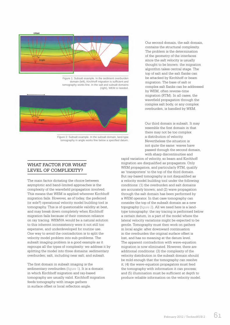
61February 2012 / TechnoHUB 2
WHAT FACTOR FOR WHAT LEVEL OF COMPLEXITY?
The main factor dictating the choice between asymptotic and band-limited approaches is the complexity of the wavefield propagation involved. This means that WEM is applied wherever Kirchhoff migration fails. However, as of today, the preferred (or sole?) operational velocity model building tool is tomography. This is of questionable validity at best, and may break down completely when Kirchhoff migration fails because of their common reliance on ray tracing. WEMVA would be a natural solution to this inherent inconsistency were it not still too expensive, and underdeveloped for routine use. One way to avoid the contradiction is to split the velocity model problem into sub-problems. The subsalt imaging problem is a good example as it regroups all the types of complexity: we address it by splitting the model into three domains: sedimentary overburden; salt, including near salt; and subsalt.
The first domain in subsalt imaging is the sedimentary overburden (figure 1). It is a domain in which Kirchhoff migration and ray-based tomography are usually valid. Kirchhoff migration feeds tomography with image gathers in surface offset or local reflection angle.
Figure 2: Subsalt example. In the subsalt domain, land-type tomography in angle works fi ne below a specifi ed datum.
Our second domain, the salt domain, contains the structural complexity. The problem is the determination of the geometry of the interfaces since the salt velocity is usually thought to be known: the migration algorithm takes central stage. The top of salt and the salt flanks can be attacked by Kirchhoff or beam migration. The base of salt or complex salt flanks can be addressed by WEM, often reverse-time migration (RTM). In all cases, the wavefield propagation through the complex salt body, or any complex overburden, is handled by WEM.
Our third domain is subsalt. It may resemble the first domain in that there may not be too complex a distribution of velocity. Nevertheless the situation is not quite the same: waves have passed through the second domain, with sharp discontinuities and
rapid variation of velocity, so beam and Kirchhoff migration are disqualified as propagators. Only WEM propagators, and particularly RTM, qualify as ‘transporters’ to the top of the third domain. But ray-based tomography is not disqualified as a velocity model building tool under the following conditions: (1) the overburden and salt domains are accurately known; and (2) wave propagation through the salt domain has been performed by a WEM operator. In that case tomography can consider the top of the subsalt domain as a new topography (figure 2). All we need here is a land-type tomography: the ray tracing is performed below a certain datum, in a part of the model where the lateral velocity variations might be expected to be gentle. Tomography must then work on gathers in local angle: after downward continuation in the overburden the original surface offset is lost, and has no meaning at the datum level. The apparent contradiction with wave-equation migration is now eliminated. However, there are additional conditions: (3) the complexity of the velocity distribution in the subsalt domain should be mild enough that the tomography can resolve it; (4) the wave-equation propagators must feed the tomography with information it can process; and (5) illumination must be sufficient at depth to produce reliable information on the velocity model.
Figure 1: Subsalt example. In the sediment overburden domain (left), Kirchhoff migration is suffi cient and
tomography works fi ne. In the salt and subsalt domains (right), WEM is needed.

62 TechnoHUB 2 / February 2012
SUBSALT EXAMPLE: APPLICATION OF TOMOGRAPHY AFTER WEM
We present here results obtained with the Sigsbee 2A synthetic dataset, courtesy of the SMAART JV. On this 2D dataset we applied a 2D WEM using a double square root (DSR) implementation of a Fourier finite difference extrapolator. This naturally produces image gathers in subsurface offset, with the specified common azimuth. We convert these gathers into the local angle domain (Sava and Fomel, 2003): the criterion of focusing of energy at zero subsurface offset becomes that of aligning the images at all angles at the same depth. The tomography we apply here is described by Adler et al. (2008). It makes use of residual moveout picked in the tangent of reflection angle (an attribute at the depth point), but is still ray-based and cannot work properly through a complex overburden. Fortunately, the conditions required to perform tomography are met below a fictitious (pseudo-) topography defined at the base of salt. Above the pseudo-topography, the overburden has
Figure 3: Sigsbee synthetic dataset. Examples of WEM image gathers: (a) image gathers in subsurface offset; (b) image
gathers converted from subsurface offset to refl ection angle in an initial velocity medium (the gathers are not fl at); (c) same
gathers after velocity update (zoomed); and (d) same gathers after velocity update (the gathers are fl attened).
exact velocities (condition 1) and the downward continuation performs (near-)exact transport (condition 2) of the seismic data to an ideal acquisition at the pseudo-topography, provided condition 5 is not a problem. Below the pseudo-topography, the medium is not too complex (condition 3) and ray-based tomography emulates correctly the wave propagation. The overburden can thus be legitimately ignored by tomography that henceforth operates only on the half-space below the pseudo-topography. Ray shooting remains confined to this half-space. In the initial model that produced the image gathers of figure 3a and b, the velocity is correct down to the base of salt. Below it, the velocities are significantly underestimated by a simple gradient. With this very simplistic starting model, a single iteration of tomographic inversion flattens the image gathers in angle (figure 3c and d).
GEOPHYSICS

63February 2012 / TechnoHUB 2
WAVE EQUATION MIGRATION VELOCITY ANALYSIS (WEMVA)
There are some cases that we cannot resolve totally with the above strategy of splitting the problem into subdomains where tomography is valid, e.g., resolution of short wavelength heterogeneity (causing residual moveouts that are difficult to pick), ensuring final consistency between a tomographically built velocity model, and band-limited propagation. Such cases call for WEMVA (Sava and Biondi, 2004; Shen and Symes, 2008), illustrated in figures 4 and 5 (p. 65 )derived from the Marmousi synthetic dataset. Figure 4a shows the initial model, and figure 4b shows the final model retrieved by WEMVA. Figure 5 compares the images obtained by migrating through the initial, WEMVA-updated and true models.
Fei et al. (2009) showed the application of WEMVA in 3D, based on common-azimuth migration, to synthetic and real datasets. The essential differences with tomography are in the back-projection operator and in the optimization criterion. Tomography uses kinematic events typically linked to picked horizons that are manipulated by ray tracing. The optimization criteria in tomography are: fit of the calculated traveltimes to the observed traveltimes (traveltime tomography), fit of traveltimes and three components of surface slowness (stereotomography), and alignment in offset or in angle at a depth point (tomography after prestack depth migration). WEMVA takes directly WEM image gathers as input, and uses WEM operators to back-project measures of the misfocusing of the seismic images. WEMVA uses full band-limited operators instead of ray tracing, hence its cost: per iteration, two full band-limited migrations plus the minimization of the cost function.
Figure 4: Application of WEMVA on an adaptation of the Marmousi synthetic dataset (courtesy of IFP): (a) initial model (smoothed version of the true model); (b) model determined by 2D shot profi le WEMVA in which short-wavelength features are retrieved.

64 TechnoHUB 2 / February 2012
DIFFERENT TYPES OF WEM IMAGE GATHERS
As stated above, WEMVA and tomography both take their input from image gathers. Tomography works with image gathers in surface offset, or in ‘true’ subsurface reflection angles (the scattering angle and the azimuth of the dip of the local reflection plane). Though traditionally these image gathers are produced by Kirchhoff or beam migration, the gathers in reflection angle can be produced directly by WEM or, more economically, derived by post-processing
The optimization criterion in WEMVA is typically (maximization of) focusing at zero subsurface offset, with the minimization of the energy imaged at non-zero-offset (differential semblance optimization, Shen et al., 2003). The two criteria, maximizing the energy of the image at zero subsurface offset and alignment within an image gather in reflection angle, are essentially equivalent, although the implementation of the gradient calculation may cause differences in convergence paths. WEMVA applied to 3D NAZ surveys can be based on common-azimuth migration so as to work on single-azimuth subsurface gathers, and benefit from the speed of common-azimuth WEM. WEMVA applied on WAZ surveys will be based on shot-profile migration or any variety of areal shot-record migration, and will work on a user-defined palette of single-azimuth, multi-azimuth, or full vector subsurface gathers.
In practice, tomography and WEMVA have complementary capabilities. On the one hand, WEMVA does not require any picking and can handle non-standard moveouts, while tomographic inversion, working with picked facets and horizons, depends on the accuracy (high-order moveout) and precision of the picks it is provided with. On the other hand, tomography can work with or concentrate on some designated picked events or horizons or a target volume. With tomography, undesirable events can be easily eliminated from the picks and all kinds of constraints and steering are easily implementable. WEMVA cannot concentrate its update on specific horizons or events, unless it is coaxed to do so by being provided with image gathers pre-processed by muting and windowing around specific events, because it has no notion of discrete events. WEMVA requires that multiples and other undesirable events have been eliminated beforehand from the seismic data.
from WEM image gathers, which can be indexed by a variety of surface and subsurface attributes. The latter can be split into those based on a focusing at zero offset and those related to local scattering angle and azimuth. Additionally, image gathers may be qualified as ‘tomo-ready’, when suitable for a tomographic update, and ‘WAZ- requiring’, if they require a WAZ input to be meaningful.
The surface attributes are simple and economical to produce. There is, for instance, the shot-point offset: the horizontal distance between the source point and the image point, defined as a scalar, hr, or as an offset vector (hx, hy). The shot point offset is ill-adapted to a tomographic update. Another type is the surface horizontal slowness at the source, which can be defined as two components (Psx, Psy) for a plane-wave, or as a single component, Psx, for a cylindrical wave. These plane or cylindrical wave attributes are usable in a tomographic update but after some adaptation of the tomographic tools.
The zero-offset subsurface attributes are available only after wavefield propagation in the subsurface. These attributes are called ‘zero-offset’ because they are extracted from the source and receiver wavefields observed at a same depth point location, as in the zero-offset imaging condition. The most readily accessible zero-offset subsurface attribute is the time-shift (focusing analysis): a relaxation of the zero-time imaging condition. This attribute is economical to produce but yields a poor resolution of the velocity update. A more desirable attribute is the local reflection angle, as obtained by direct decomposition of the source and receiver wavefields at the depth point (Soubaras, 2003; Xie and Wu, 2002). Nevertheless, it is extremely expensive and cumbersome to produce. Another sort of zero-offset attribute would be the scaling or scanning factor of the velocity scan, but it is not very economical either. These gathers can be adapted to a tomographic update.
Most of the other subsurface attributes are based on the subsurface offset. The subsurface offset can be considered as the offset after datuming in the vicinity of the image point. At the subsurface CMP location, we produce for every shot and every subsurface offset (hx, hy) the cross-correlation in time of the source and receiver wavefields. This yields a datumized field in time (hx, hy, t). One option is to convert this subsurface offset into the subsurface offset ray-parameter (Phx, Phy). The further conversion into gathers in reflection angle is possible but cumbersome, as it requires the knowledge of the local dip and the local velocity.
GEOPHYSICS

65February 2012 / TechnoHUB 2
The commonplace approach uses directly the migrated gathers in subsurface offset, obtained by taking the zero-time sample of the cross-correlated field, (hx, hy, t = 0). Sava and Fomel (2003) proposed formulae for the conversion, per azimuth line, from subsurface offset to an approximation of the reflection angle assuming a local 1D medium, without requiring the local velocity and reflector dip. These gathers are considered as the best compromise because they are quite economical and are usable in a tomographic update.
IMPORTANCE OF WAZ ACQUISITION FOR MEANINGFUL WEM IMAGE GATHERS
The surface attributes can be filtered by the acquisition parameters, so they are generally applicable to both NAZ and WAZ surveys. In contrast, the subsurface attributes are available only after wavefield propagation in the subsurface. At the stage of producing the image gathers, specific information on the acquisition parameters (surface offset, azimuth, and aperture) has been lost, but
the acquisition imprint and illumination problems are transmitted all the same to the image gathers and the stack image. In the subsurface attributes, there is either an implicit summation over all azimuths, or the strong assumption that the entire azimuth information is available at the depth point. The zero-offset attributes, for instance, generally ignore whether the acquisition is WAZ rather than NAZ and assume an implicit summation upon all propagation azimuths reaching the image point.
In the case of the subsurface attributes derived from the subsurface-offset (hx, hy), we assume in general that the datumed wavefield captured at every depth point contains meaningful specular information along all the directions. A necessary condition for this assumption to be valid is that the original acquisition be full-azimuth at the surface.
During the surface-to-depth wavefield propagation, any azimuth acquired at the surface will be twisted and mapped to another specular azimuth at a given depth location. In order to be sure to get any desired specular azimuth at the observation depth location, it seems necessary to have available all the azimuths at the surface. It might not be sufficient in all cases though, as blind zones in the surbsurface might remain poorly illuminated even with fine sampling in azimuth.
fi gure 5: Application of WEMVA on the Marmousi synthetic dataset: (a) image obtained with the initial
model (smoothed version of the true model); (b) image obtained with the WEMVA updated velocity
model; and (c) image obtained with the exact model.

66 TechnoHUB 2 / February 2012
Figure 6: Image gather in subsurface offset for a horizontal refl ector in a homogeneous medium (courtesy F.Gao): (a) and (d) intersection of crossline offset plane hx = 300 m with inline offset plane hy = 0; (b) and (e) intersection of crossline offset plane hx = 0 with inline offset plane hy = 0; (c) and (f) intersection of crossline offset plane hx = 0 with inline offset plane hy = 300 m. In (a) – (c) for WAZ acquisition, the quality of focusing at zero subsurface offset depends on the available aperture in depth. In (d) – (f) for single cable acquisition, there is no focusing in the crossline offset direction and the corresponding artefact should not be incorporated in velocity analysis.
GEOPHYSICS

67February 2012 / TechnoHUB 2
One expected uplift from having WAZ data as input is that we may choose the observation azimuths in the subsurface. In that case, we can output only single azimuthal subset lines from the (hx, hy) grid, for instance, the pure inline (all hx, hy = 0) or the pure crossline (hx = 0, all hy) subsurface offsets, thus limiting drastically both the cost and the volume of the image gathers. Note that NAZ data will entail severe limitations: to grab the specular azimuth as mapped to depth, either we would have to resort to common-azimuth propagation, constraining unphysically the subsurface specular azimuth to be equal to the acquisition azimuth, or we would have to perform a cumbersome and costly post-migration search for the specular azimuth in the entire subsurface offset volume (hx, hy).
To illustrate the importance of illuminating a specular azimuth, we take a canonical example of image gathers in subsurface offset. For a flat horizontal reflector in a constant velocity medium, we emulate single cable (6.4 km length) and
ConclusionWe described two velocity model building strategies involving WEM. In the first strategy, making use of the existing tomographic tools, the problem is split into subdomains where the local velocity update from tomography is valid. A second strategy is to use WEMVA, which is naturally associated with WEM. However, it is still expensive for routine use, and methodologies are, as yet, relatively undeveloped. WEMVA can be applied after the first strategy, or wherever it fails. In both strategies, WEM image gathers are supplied as input to tomography and WEMVA, respectively. We described several type of image gathers produced by WEM, and discussed particularly their suitability as input tomography. We suggest that WAZ surveys add significant value to WEM image gathers in terms of reliability and flexibility.
REFERENCES
Adler, F., Baina, R., Soudani, M.A., Cardon, P. and Richard, J.B. [2008]Non linear 3D tomographic least-square inversion of migrated depth in Kirchhoff PreSDM common-image gathers. Geophysics, 73, VE1-VE23.
wide-azimuth (swath 2 km, cable 6.4 km) acquisition and produce image gathers in subsurface offset (hx, hy) at a full-fold image location at the centre of the survey. Figures 6a, b and c show the image gather for the WAZ experiment. Figures 6a and b show the intersection of a finite crossline offset planes (hx = 300 m and hx = 0) with inline offset plane hy = 0. We can observe a clear focus along hx in the vicinity of hx = hy = 0. Figures 6b and c show the intersection of the constant crossline offset plane hx = 0 with inline offset planes hy = 0 and hy = 300 m. We see that the focus along hy in the vicinity of hx = hy = 0 is not as clearly defined, because of the smaller available aperture (2 km crossline instead of 6.4 km inline), proving once more the importance of aperture on resolution. Figures 6d, e and f show the same plots as figures 6a, b and c, but for the single cable experiment. In the inline subsurface offset (figure 6d), nothing changes, while in the crossline offset (figures 6e and f), we have a pure truncation artefact. Needless to say, this truncation artefact, corresponding to a non-specular azimuth, should be neither picked nor taken into account in the WEMVA cost function.
Fei, W., Williamson, P. and Khoury, A. [2009] 3-D common-azimuth migration velocity analysis based on FFD source-geophone implementation and differential semblance optimization. 79th SEG Annual Meeting, Expanded Abstracts, 28, 2283-2286.
Pratt, R.G., Song, Z.M., Williamson, P.R. and Warner, M.R. [1996] Two-dimensional velocity models from wide angle seismic data by waveform inversion. Geophysical Journal International, 124, 323-340.
Sava, P. and Biondi, B. [2004] Wave-equation migration velocity analysis, Parts I-II. Geophysical Prospecting, 52, 593-623.
Sava, P. and Fomel, S. [2003] Angle-domain common-image gathers by wavefi eld continuation methods. Geophysics, 68, 1065-1074.
Shen, P., Stolk, C. and Symes, W. [2003] Automatic velocity analysis by differential semblance optimization. 74th SEG Annual Meeting, Expanded Abstracts, 22, 1709-1712.
Shen, P. and Symes, W.W. [2008] Automatic velocity analysis via shotprofi le migration. Geophysics, 73, VE49-VE59.
Soubaras, R. [2003] Angle gathers for shot-record migration by local harmonic decomposition. 73rd SEG Annual Meeting, Expanded Abstracts, 22, 889-892.
Xie, X.B. and Wu, R.S. [2002] Extracting angle domain information from migrated wavefi eld. 72nd SEG Annual Meeting, Expanded Abstracts, 21, 1360-1363.
Received 30 September 2009; accepted 22 February 2010.

68 TechnoHUB 2 / February 2012
The deeper the field, the more difficult it is to position the wells.
Classically, data acquired during seismic surveys provide a time-migrated image of the subsurface, before conversion to a depth image, generally using a velocity field based on well data. This so-called "depth migration" transformation is more useful, particularly for drillers, for accurate depth positioning of the wells. The technique called “prestack” is now commonly used to retain a maximum number of data on a field, compared to the standard technique in which all rays arriving at a single point are summed and averaged. The prestack technique is known to provide the best imaging and positioning if a fine velocity field is established.
Prestack processing was performed at the same time as the traditional time imaging to position the wells on the gas condensate fields of Elgin-Glenelg-Franklin, at depths greater than 5,000 m. The main objective was to enhance the positioning accuracy.
CONTEXT
Geologically, the layers are mainly flat and horizontal down to the BCU (Base of Cretaceous Unconformity) located around 5,000 m depth. Below, tilted blocks are the petroleum traps.
Unfortunately, the results were disappointing, especially in the Northern part of the field, where the time-migrated image was locally better. At these locations, glacial channels about 1 or 2 km wide were identified between the sea bed (about 100m depth) and 500m depth.
This created the need to repeat the complete seismic processing, this time including the channels in the velocity model. The final result was greatly improved, particularly over the deeper petroleum targets, as explained in the following article.
GEOPHYSICS
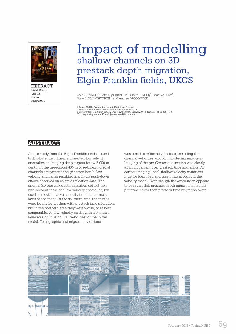
69February 2012 / TechnoHUB 2
Impact of modelling shallow channels on 3D prestack depth migration, Elgin-Franklin fields, UKCS
A case study from the Elgin-Franklin fields is used to illustrate the influence of seabed low velocity anomalies on imaging deep targets below 5,000 m depth. In the uppermost 400 m of sediment, glacial channels are present and generate locally low velocity anomalies resulting in pull-up/push-down effects observed on seismic reflection data. The original 3D prestack depth migration did not take into account these shallow velocity anomalies, but used a smooth interval velocity in the uppermost layer of sediment. In the southern area, the results were locally better than with prestack time migration, but in the northern area they were worse, or at best comparable. A new velocity model with a channel layer was built using well velocities for the initial model. Tomographic and migration iterations
were used to refine all velocities, including the channel velocities, and for introducing anisotropy. Imaging of the pre-Cretaceous section was clearly an improvement over prestack time migration. For correct imaging, local shallow velocity variations must be identified and taken into account in the velocity model. Even though the overburden appears to be rather flat, prestack depth migration imaging performs better than prestack time migration overall.
Jean ARNAUD1*, Lotfi BEN-BRAHIM2, Claire TINDLE2, Sean VARLEY2, Steve HOLLINGWORTH 3 and Andrew WOODCOCK 3
1 Total, CSTJF, Avenue Larribau, 64000, Pau, France.2 Total, Crawpeel Road Altens, Aberdeen, AB 12 3FG, UK.3 CGGVeritas, Crompton Way, Manor Royal Estate, Crawley, West Sussex RH 10 9QN, UK.*Corresponding author, E-mail: [email protected]
EXTRACTFirst BreakVol 28Issue 5May 2010
ABSTRACT

70 TechnoHUB 2 / February 2012
LOCATION OF THE STUDY AND STRUCTURAL DESCRIPTION
The Elgin, Franklin, Glenelg, and West Franklin fields are located within the Central Graben in the UK part of the North Sea (figure 1). The bedding is flat down to the Base Cretaceous Unconformity (BCU). Below, tilted fault blocks provide the traps for the gas condensate fields (figure 2a).
In the Tertiary section, above the Balder Formation, alternating sand and shale sequences are present, resulting in locally anisotropic formations. In the Cretaceous section, between the blue horizon at 3.5 km depth and the BCU (figure 2a), shale and limestone sequences are present. The sonic log (figure 2b) shows great variation in velocity. Interval velocities in the Tertiary are around 2,000 m s-1, and reach values in the range 5,000–6,000 m s-1 in the Cretaceous Chalk section. The Balder seismic event marks a major increase in acoustic impedance. There are major downward steps in acoustic impedance at the base of the Chalk, below 5,000 m depth.
INTRODUCTION
Low-velocity channels located close to the sea bottom can cause important distortions of the velocity field if the length of the acquisition spread is larger than the size of the anomaly. This phenomenon is well known when processing seismic data in time, and causes oscillations in the stacking velocities. A ‘push-down’ effect is often associated with these features. In the time domain, a common way to correct them is to apply static corrections based either on picking the channels or simply by flattening a reference horizon just below the anomalies. This static correction approach does not really solve the velocity problem: it merely provides seismic horizons with geometries closer to what is perceived as the true geological layering.
In the depth domain, the channels must be included in the velocity model to achieve an accurate migration of the seismic data below them. Here we present a case study where this problem was identified and solved. We compare prestack depth-migrated data processed using a velocity model with and without shallow channels. The benefit of including these features in the velocity model is evident from the improvement in data quality.
Figure 1: Elgin-Franklin fi elds location map.
PRESTACK DEPTH MIGRATION (PSDM)
The PSDM was performed following a standard layerstripping approach. As the sonic logs exhibit strong positive and negative velocity contracts (figure 2b), 15 horizons were picked on the time-migrated data to take these variations into account. Sonic and VSP logs were available for 15 wells. Using all wells, an initial model was built with an interval velocity function determined for each interval using linear regression:
Vint =V0 + kz, (1)
where Vint is interval velocity, z is depth, and V0 and k are constants. The initial model was used for the first migration. Then an iterative tomographic approach was used to update the velocity model following optimization of the velocity function in each layer, working from the top downwards. Anisotropy was introduced to tie the wells in depth as a final step in dealing with each layer. It also improved the flattening of the common image-point gathers at all offsets.
The following methodology was used, based on Thomsen’s VTI approximations (Thomsen 1986):
▪ Calculate the values of V0 and k that best flatten common image-point gathers.
▪ Accurately calibrate the well marker associated with the horizon at the base of the layer. (Check geological marker on logs, and use the well tie to check the seismic phase of the horizon).
GEOPHYSICS

71February 2012 / TechnoHUB 2
MAIN ISSUES WITH THE DEPTH IMAGING
Over the southern part of the 3D survey area, the quality of the depth image was considered to be better than the PSTM image, except over those areas where it was anticipated that the velocity model might be too smooth. Over the northern part, the quality was fair, comparable to the PSTM image. However, the depth image was locally worse than the PSTM image (figure 3). The event (fault or salt interface) below the tilted blocks was better imaged on the PSTM. The amplitude of the folding around the shallow Plenus Marl marker horizon (around 5 km depth, or 4 s two-way time) is larger on the PSDM than on the PSTM. An under-corrected velocity effect is suspected over this location, which could explain the deteriorated imaging below.
Figure 2 (a): Example of the structure visible on a depth migrated line. (b) Sonic log from 1 km depth to TD in the well located on the section shown in (a).
▪ Calculate the delta coefficient by comparing the seismic layer thickness to its well thickness.
▪ Average delta for the 15 wells, excluding outliers when judged to be necessary.
▪ Scale the vertical velocity to maintain the gather flatness.
▪ Calculate the epsilon coefficient which provides the best flattening of the far offset traces.
▪ New tomographic update to refine the velocities.
This method is thus applied layer by layer, from the top downwards. Note that each seismic layer is tied to wells and corrected in an average sense. The method is valid only for transversely isotropic horizontal layers (the VTI approximation), which is a valid assumption for the Elgin-Franklin fields at least down to the BCU. After about nine months of processing, the depth cube was delivered to the interpreters.
In the upper layers, the same phenomenon is observed around 3 km depth, or 3 s two-way time. Figure 4 (p. 72) shows a time section and two picked horizons, M24 at about 2.4 s or 2,250 m, and the Balder at about 3 s or 3,000 m. The corresponding depth horizons are also displayed to highlight a possible velocity effect. In this area, the average velocity is close to 2,000 m s-1, so the time horizon in milliseconds is equivalent to depth in metres. At M24, time and depth horizons are conformable, although slightly diverging locally due to minor lateral velocity variations. At Balder level, they are still parallel on the right side of the section, but diverge on the left side where the geometry of the depth horizon clearly differs from the time horizon. We conclude that the velocity field is varying laterally between M24 and Balder with no obvious geological clue evident on the section as to the origin of the variation.
Figure 3: Comparison between PSDM and PSTM over the northern part of the 3D survey area.
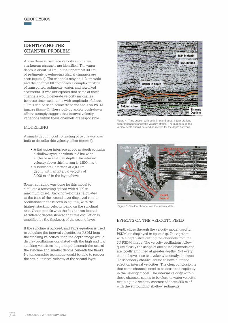
72 TechnoHUB 2 / February 2012
Figure 4: Time section with both time and depth interpretations superimposed to show the velocity effects. The numbers on the vertical scale should be read as metres for the depth horizons.
IDENTIFYING THE CHANNEL PROBLEM
Above these subsurface velocity anomalies, sea bottom channels are identified. The water depth is about 100 m. In the uppermost 400 m of sediments, overlapping glacial channels are seen (figure 5). The channels may be 1–2 km wide and the channel fill comprises a complex mixture of transported sediments, water, and reworked sediments. It was anticipated that some of these channels would generate velocity anomalies because time oscillations with amplitude of about 10 m s can be seen below these channels on PSTM images (figure 6). These pull-up and/or push-down effects strongly suggest that interval velocity variations within these channels are responsible.
MODELLING
A simple depth model consisting of two layers was built to describe this velocity effect (figure 7):
▪ A flat upper interface at 500 m depth contains a shallow syncline which is 2 km wide at the base at 900 m depth. The interval velocity above this horizon is 1,500 m s-1.
▪ A horizontal interface at 3,000 m depth, with an interval velocity of 2,000 m s-1 in the layer above.
Some raytracing was done for this model to simulate a recording spread with 4,000 m maximum offset. Stacking velocities calculated at the base of the second layer displayed similar oscillations to those seen in figure 6, with the highest stacking velocity being on the synclinal axis. Other models with the flat horizon located at different depths showed that this oscillation is amplified by the thickness of the second layer.
If the syncline is ignored, and Dix’s equation is used to calculate the interval velocities for PSDM from the stacking velocities, then the depth image would display oscillations correlated with the high and low stacking velocities: larger depth beneath the axis of the syncline and smaller depths beneath the flanks. No tomographic technique would be able to recover the actual interval velocity of the second layer.
Figure 5: Shallow channels on the seismic data.
EFFECTS ON THE VELOCITY FIELD
Depth slices through the velocity model used for PSDM are displayed in figure 8 (p. 74) together with a depth slice cutting the channels from the 3D PSDM image. The velocity oscillations follow quite closely the shape of one of the channels and are locally amplified at greater depths. Not every channel gives rise to a velocity anomaly: on figure 8 a secondary channel seems to have a limited effect on interval velocities. The clear conclusion is that some channels need to be described explicitly in the velocity model. The interval velocity within these channels seems to be close to water velocity, resulting in a velocity contrast of about 300 m s-1 with the surrounding shallow sediments.
GEOPHYSICS

73February 2012 / TechnoHUB 2
Figure 7: Two-layer model and associated stacking velocities.
IMPLEMENTATION OF A NEW DEPTH PROCESSING WORKFLOW
As these channels are quite shallow, the range of available offsets at their bases is limited and the corresponding stacking velocities are commonly not reliable for calculating interval velocity using Dix’s equation: maximum depth is about 600 m, maximum offset 600 m, and water depth about 100 m. To appraise the interval velocity in these channels, two options are available: retrieve information at deeper layers using pull-up/push-down effects (evident in figure 6) or through the oscillating impact on stacking velocities as shown on the model in figure 7. These two options are complementary as pull-up/push-down effects become less clear with increasing depth, while the stacking velocity oscillations are amplified. Velocity and anisotropy variations for the deeper layers must also be appraised. It was decided to put the channels into the initial model before the tomographic update.
PROCESSING WORKFLOW
The workflow is as follows:
1. The velocity model output for the original PSDM had too many lateral velocity variations due to the channel effects. The well velocity logs were revisited and a smooth model derived from them. This model included a rough estimate of anisotropy. A depth migration was performed with the smoothed model down to a depth of 2,000 m.
2. A horizon located as close as possible to the base of the channels was picked in depth (M5 in figure 6). This horizon was smoothed using a 3 km radius to provide an estimate of the undisturbed horizon geometry (figure 9 p. 74). An alternative solution would have been to pick a smoothed horizon manually.
Figure 6: Example of surface channels imaged on a line processed with PSTM.
3. The depth difference between the smoothed and the initial picks was vertically converted into adjusted interval velocities within the uppermost layer of sediment between the seabed and M5.
4. PSDM was performed down to 7,000 m.
5. Long-wavelength variations in the velocity field were tomographically updated from the seabed to the Balder. Anisotropy was then adjusted and kept constant in each of these layers.
6. The channel modelling step was then repeated. Geostatistical filtering (factorial kriging) was used to isolate the residual depth distortions resulting from the shallow channels. Depth picks were vertically converted to velocity and placed in the interval from the seabed to M5.
7. Short wavelength variations in the velocity field were tomographically updated from the seabed to a mid - Tertiary horizon at about 1,300 m depth. During this update the tomographic process was allowed to update those cells within the interval from the seabed to M5.
8. Long-wavelength variable anisotropy was introduced tomographically between the seabed and the mid-Tertiary horizon.
9. A short-wavelength tomographic update of the velocity field was then performed between the mid-Tertiary and Balder horizons.
10. Long-wavelength variable anisotropy was introduced tomographically between the mid-Tertiary and Balder horizons.
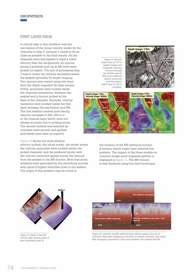
74 TechnoHUB 2 / February 2012
FIRST LAYER ISSUE
A critical step in this workflow was the calculation of the initial velocity model for the channels in step 3, because it needs to be as close as possible to the final results. As the channels were anticipated to have a lower velocity than the background, all options giving a potential pull-up at M5 level were picked (in depth). The aim of processing step 3 was to locate the velocity anomalies below the seabed optimally for depth imaging. Two options were tested using test lines from the depth-migrated 3D data volume. Firstly, anomalies were located inside the channels themselves, between the seabed and a horizon picked at the base of the channels. Secondly, velocity variations were located inside the first layer between the sea bottom and M5. The first method created quite strong velocity contrasts of 200–300 m s-1 in the channel layer which were not always accurate due to picking errors. The second method was selected as contrasts were smooth and gathers and stacks were seen as superior.
Figure 10 shows the three shallow velocity models, the initial model, the model where the velocity anomalies were located within the picked channels, and the preferred model with the velocity variations spread across the interval from the seabed to the M5 horizon. Note that some artefacts were generated by the smoothing process, with spots of higher velocities close to the seabed. The origin of this problem may be errors in
Figure 8: Seismic depth slice at 170 m
(upper image) and composite overlays
of slices through the PSDM velocity
fi eld at two different depths (coloured)
and the seismic depth slice at 170 m
(shaded).
Figure 9: Depth of the M5 horizon after picking (step 2) and smoothing (step 3).
Figure 10: Velocity models obtained (top) without taking account of channels; (left) after assigning corrections to picked channels; and (right) after assigning corrections to the layer between the seabed and M5.
the location of the M5 reference horizon. A horizon repick might have reduced this problem. The impact of the three models on common image-point migrated gathers is displayed in figure 11. The M5 horizon is best flattened using the third technique.
GEOPHYSICS

75February 2012 / TechnoHUB 2
LAYER BELOW THE CHANNELS
PSDM stack sections are compared in figure 12. At the M5 level, oscillations have disappeared from the image produced by the new workflow, as expected since all corrections were calculated with a smoothed M5. Furthermore, the oscillations on the M10 horizon are greatly reduced. Note that there are no differences below the M5 horizon in the velocity fields used to generate these stack sections. The differences between the images are less clear for horizons underlying M10.
The gathers located over the channels exhibit an interesting behaviour: the introduction of the channel layer changes the moveout (figure 13). Consideration of figure 14 (p. 76) explains this effect. When the channels are not defined in the model, the short offset migration velocity is higher than the true one, and
Figure 11: Migrated gathers for (left) initial velocity model; (middle) velocity anomalies assigned within channels; and (right) velocity anomalies assigned to the layer between the seabed and M5.
Figure 12: Comparison of PSDM stack sections (left) before and (right) after channel velocity correction.
Figure 13: Comparison of migrated depth gathers, before and after channel correction with a zoom on the right. The maximum offset is 4,600 m.
depths are higher. As the far offsets are not in the anomaly, their associated velocity and their depths are not affected. Inserting a slower velocity in the channel decreases the moveout on deeper horizons.
The preferred model with the velocity variations spread across the interval from the seabed to the M5 horizon was input into the new processing workflow at step 3. Figure 15 (p. 76) shows the effect on the final velocity field above the Balder horizon at around 3 km depth. The oscillations seen on previous velocity models between 2 and 3 km depth are no longer present. Some minor velocity variations are present between 3 and 3.2 km. However, an additional PSDM iteration for refining the channel velocities was not deemed necessary.

76 TechnoHUB 2 / February 2012
Figure 14: Sketch of raypaths through and outside the channel anomaly.
Figure 15: Velocity model obtained (left) without and (right) with channel velocities in the model.
FINAL RESULTS (PSDM STACK)
Figure 16 shows the final migration results after tomographic refinement of velocities and calibration of anisotropy down to Jurassic level. No post-migration processing has been applied. The two sections were derived using different anisotropies and velocities for PSDM, but both were processed with the same quality control criteria for prestack depth imaging: gather flattening,
Figure 16: Line 800. Comparison of fi nal depth sections (left) without and (right) with channels in the velocity model.
Figure 17: Line 520. Comparison of fi nal depth sections (left) without and (right) with channels in the velocity model.
PSDM AND PSTM
It is common practice to compare the result of PSDM after stretching the depth axis into time with the PSTM image. They are very similar above the BCU (figure 18). Over the northern part of the survey area, where seabed channels are present, the PSDM image below the BCU appears slightly better than the PSTM. Lateral displacements of about 100 m can be seen. Figure 19 and figure 20 show zooms of lines 800 and 720 at the level of the targeted structures. On line 800, the PSDM image is clearer below the BCU. On line 720, the PSDM image is sharper, and the faults are better defined.
Figure 21 shows the same comparison for a line located below the edge of the channel in the Franklin area. The differences are variable: on the PSDM image, reflectors at BCU level and faults are more continuous. Over the Franklin Field, which is the horst feature in the middle, the differences are minor.
good well tie, no artificial oscillations in the velocity field, nor in the reflector geometry. The improvement in the image quality of the tilted blocks and the fault planes is clear.
Figure 17 shows the same comparisons for depth sections on line 520 (Franklin location). There is again an improvement in the reflector geometry just below the BCU.
GEOPHYSICS

77February 2012 / TechnoHUB 2
Figure 18: Line 800. PSDM and PSTM comparison after post-processing and conversion of the vertical scale to time for the PSDM section.
Figure 19: Zoomed comparison of PSDM converted to time and PSTM for line 800.
Figure 20: Zoomed comparison of PSDM converted to time and PSTM for line 720.
Figure 21: Zoomed comparison of PSDM converted to time and PSTM for line 520.
ConclusionsThe North Sea case study presented here shows the importance of correcting for seabed channel velocity anomalies when imaging deep targets (down to 7 km in this case). Ignoring the need for such corrections degrades the quality of the seismic image at the target level. The methodology used to correct for these channels involved additional tomographic updates of the interval velocity field to separate channel effects from genuine velocity and anisotropy variations in the deeper layers.
ACKNOWLEDGEMENTS For permission to present this material, we would like to thank Total management and Elgin-Franklin fi elds coventurers, Eni, BG Group, GDF, Ruhrgas, Chevron, Exxon- Mobil, Dyas, and Oranje-Nassau. The depth processing was performed by CGGVeritas in Crawley, UK.
REFERENCE
Thomsen, L. [1986] Weak elastic anisotropy. Geophysics, 51, 1954-1966.
Received 4 May 2009; accepted 12 March 2010.

78 TechnoHUB 2 / February 2012
In order to identify prospects or characterize reservoirs, geoscientists often rely primarily on seismic images based on the propagation of waves in the subsurface. However, in the case of complex subsurface geology, these images can be severely degraded. Recent developments in seismic imaging have dramatically improved the image quality, although in some cases the improvement is not sufficient to allow an unambiguous interpretation and artifacts may still be present. These artifacts can be due to the limits of the dataset, to physical phenomena related to wave propagation in complex media, or to the methods used to produce the image from the data.
The topic of this article is the use of seismic modelling to test an interpretation. Modelling is a common tool for seismic survey design, but here it has been used to determine the origin of some seismic events observed on images. The case studied in this paper is a prospect located below a salt canopy in the deep offshore Gulf of Guinea. Observations from different datasets sometimes led to different
interpretations, none of them consistent with all the observations. This diminished the likelihood of success of the prospect and resulted in more uncertainty as to its potential resources.
The modelling performed in this case produced images that could be directly compared to actual data. This greatly helped us to understand why the images were different. More importantly, it showed that the differences could well be compatible with one of the interpretations despite seemingly conflicting observations. This resulted in a better appraisal of the risk of the prospect and its potential resources.
GEOPHYSICS
CONTEXT
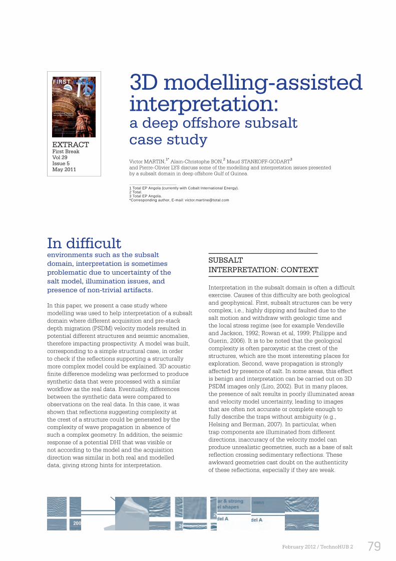
79February 2012 / TechnoHUB 2
3D modelling-assisted interpretation: a deep offshore subsalt case studyVictor MARTIN,1* Alain-Christophe BON,2 Maud STANKOFF-GODART3 and Pierre-Olivier LYS discuss some of the modelling and interpretation issues presented by a subsalt domain in deep offshore Gulf of Guinea.
1 Total EP Angola (currently with Cobalt International Energy).2 Total.3 Total EP Angola.*Corresponding author, E-mail: [email protected]
In difficult environments such as the subsalt domain, interpretation is sometimes problematic due to uncertainty of the salt model, illumination issues, and presence of non-trivial artifacts.
In this paper, we present a case study where modelling was used to help interpretation of a subsalt domain where different acquisition and pre-stack depth migration (PSDM) velocity models resulted in potential different structures and seismic anomalies, therefore impacting prospectivity. A model was built, corresponding to a simple structural case, in order to check if the reflections supporting a structurally more complex model could be explained. 3D acoustic finite difference modeling was performed to produce synthetic data that were processed with a similar workflow as the real data. Eventually, differences between the synthetic data were compared to observations on the real data. In this case, it was shown that reflections suggesting complexity at the crest of a structure could be generated by the complexity of wave propagation in absence of such a complex geometry. In addition, the seismic response of a potential DHI that was visible or not according to the model and the acquisition direction was similar in both real and modelled data, giving strong hints for interpretation.
SUBSALT INTERPRETATION: CONTEXT
Interpretation in the subsalt domain is often a difficult exercise. Causes of this difficulty are both geological and geophysical. First, subsalt structures can be very complex, i.e., highly dipping and faulted due to the salt motion and withdraw with geologic time and the local stress regime (see for example Vendeville and Jackson, 1992; Rowan et al, 1999; Philippe and Guerin, 2006). It is to be noted that the geological complexity is often paroxystic at the crest of the structures, which are the most interesting places for exploration. Second, wave propagation is strongly affected by presence of salt. In some areas, this effect is benign and interpretation can be carried out on 3D PSDM images only (Liro, 2002). But in many places, the presence of salt results in poorly illuminated areas and velocity model uncertainty, leading to images that are often not accurate or complete enough to fully describe the traps without ambiguity (e.g., Helsing and Berman, 2007). In particular, when trap components are illuminated from different directions, inaccuracy of the velocity model can produce unrealistic geometries, such as a base of salt reflection crossing sedimentary reflections. These awkward geometries cast doubt on the authenticity of these reflections, especially if they are weak.
EXTRACTFirst BreakVol 29Issue 5May 2011

80 TechnoHUB 2 / February 2012
Moreover, artifacts resulting from wave propagation or processing are sometimes difficult to clearly evidence due to their similarity to complex structural elements that are seen in many subsalt areas and wells. For instance, highly dipping events could either be tails of diffraction hyperbolas or true reflections. In this situation, the interpreter can be left with different possibilities that lead to severe differences of gross rock volume estimation, different risk assessments and different optimal well implantation. Several approaches can help resolving this issue. Structural analysis, using simple concepts (Martin et al., 2010) or implying 3D restoration, can help ruling out inappropriate models. However this task can be extremely difficult to execute in 3D complex subsalt domains, as it often has to be performed at a scale much exceeding the size of the prospect. Intensive effort on reprocessing or new acquisition can also enhance seismic images, reducing the uncertainty. In some cases, however, uncertainty remains even after heavy seismic work. Eventually seismic modelling, which is a powerful tool for acquisition design (e.g., Regone, 2007) can also be used to help the understanding of artifacts on an image. Liao et al. (2009a) for instance presented a case where modelling evidences distortions created by a fault on PSTM images. Liao et al. (2009b) showed modelling could explain results of a subsalt well that were inconsistent with seismic images. In this paper, we present a case of a subsalt structure insufficiently seen on PSDM images prior to drilling, where geometry was de-risked with the help of 3D seismic modelling.
CASE PRESENTATION: DEEP OFFSHORE GULF OF GUINEA
The case studied lies in deep offshore Gulf of Guinea, in a compressive domain where salt formed prominent canopies. The overall structure is a tilted thrusted panel bounded by salt, evidenced by early PSDM images in the area. This tilted panel is mainly subsalt with only part of its crest sitting below a saltfree window. Two narrow-azimuth acquisitions were performed over the area in 2000 and 2007 with two different acquisition directions. Different salt interpretations also led to different velocity models that were used to migrate the two datasets (Martin et al., 2007, Sexton et al., 2009). In this case, we only describe the two most likely models, which have been widely used for interpretation. The most significant difference between the two models is the geometry of the salt nose above the structure. In one case (model A), the salt nose is simple, whereas in the other case (model B) an overhang is present due to several episodes of salt motion. Both salt geometries could be supported from different geological evidences, and seismic images alone do not allow discrimination between these two models.
Two acquisitions and two models result in four different imaging combinations that were applied to produce an image of this structure (figure 1), and even more if we consider that several migration techniques were used. These different imaging combinations lead to different interpretations. On the 2000A dataset (2000 data, salt model A, see figure 1), the structure appears to be a simple tilted panel against the salt with no apparent crestal complexity. Furthermore, a flat seismic anomaly (FSA) can be spotted across part of the sedimentary section. On the 2000B dataset, the structure is less clear at the crest. The FSA is smeared, and the area where it is actually flat is much more restricted than on the 2000A image. It can only be seen over part of the area where it is present in 2000A data, below unambiguously interpreted salt. 2007A and 2007B datasets show complex reflections at the crest suggesting the presence of a small perched basin above a crestal backthrust. However, the shape of the reflections could also suggest that they are actually artifacts smearing on one side of a narrow salt-free window (figure 1). The seismic anomaly is not present on these 2007 datasets. Therefore, we end up with two different structural models to describe the crest of the structure (figure 2) and a seismic anomaly that is present or absent depending on the data and model used. The latter point is problematic, because usual quantitative criteria employed for direct hydrocarbon indicator (DHI) evaluation are often unavailable in subsalt domains.
Figure 1: Seismic profi les at the same location in different seismic cubes obtained by wave-equation migration (WEM). Labelling corresponds to the 2000 (~dip) or 2007 (~strike) acquisitions, the letter corresponds to the velocity model used for migration (velocity models A and B).
GEOPHYSICS

81February 2012 / TechnoHUB 2
MODEL CONSTRUCTION
The structure itself and the overlying salt being all but cylindrical, we decided to perform acoustic modelling in three dimensions. This choice, although ensuring a better result, was not straightforward, as it had a significant impact on planning and cost. Acoustic modeling requires both a velocity and a density model to be input. For the sake of comparison, we wanted to stay as consistent as possible with model A from a kinematic point of view. Therefore, we kept the migration velocity model A (figure 3, top p. 82) as the P-wave velocity model for the acoustic modelling. This model correctly expresses a velocity contrast at the salt/sediment boundary. However, the drawback of using the migration velocity is that the velocity field is in this case smooth outside the salt bodies and homogeneous inside the salt, so it does not feature any other impedance contrast than sea bottom and salt/sediment interfaces.
In this situation, one could be tempted to choose the image that best fits a purpose and ignore the other ones, based on the similarity of ignored reflections to artifacts. However, one of the lessons from drilling in this type of environment is that it is often wrong to discard reflections simply because they don’t match a model, as they sometimes turn out to be true indications of subsurface complexity and not artifacts as generally thought. Furthermore, many structures in this type of environment are bowl-shaped and have the appearance of migration smiles.
In the end, and despite strong acquisition and processing efforts, we were not able to fully describe the structure at an acceptable risk level. Furthermore, the seismic anomaly lacked consistency on the different datasets to be called a robust DHI. This type of issue unfortunately arises in many cases when dealing with multiple seismic cubes in challenging exploration environments like subsalt domains, where both salt geometry and subsalt velocity are not sufficiently constrained.
In this case, without knowing if the cross-dipping reflections suggesting a possible backthrust were true primary reflections or artifacts, the structure could not be confidently described. Regarding the flat seismic anomaly, it was inconsistent between the different cubes and thus difficult to be called a DHI, unless we could show that it was normal not to see it on most of the seismic cubes. Therefore, in order to test whether our preferred model (model A) could explain why these four datasets showed such dissimilarities, we carried out a modelling study. This study was aimed at answering two precise questions, to help address the interpretation issues: Can reflectors corresponding to the simple thrusted panel model (figure 2 top) create artifacts suggesting presence of a fault in a certain acquisition direction? Can the presence/absence of the seismic anomaly be explained by the use of a given model and acquisition direction?
To answer these questions, we used a workflow consisting of: building an acoustic model from the simple thrusted structural model; introducing a fluid contact at the seismic anomaly location; generating two datasets according to the two acquisition directions; processing and migrating the two datasets with the two velocity models; and comparing the result with observations on real data. This process is thoroughly described in the following sections. Figure 2: Schematic structural models corresponding to
observations made on 2000 seismic that lead to a simple tilted panel interpretation (top) and 2007 seismic suggesting a backthrust at the crest of the structure (bottom).

82 TechnoHUB 2 / February 2012
MODELLING AND MIGRATION
The two narrow azimuth seismic acquisitions performed over the area of interest in 2000 and 2007 were simulated using Total’s in-house 3D acoustic modelling code (Tarrass et al., 2008). In order to save computation time, we used a source with a lower bandwidth than the real data with a peak frequency at 12 Hz, not far from the peak frequency of the real data in the subsalt domain, but a maximum frequency of only 30 Hz, which is lower than the maximum frequency previously used to migrate the real data (37 Hz). This maximum frequency implies a minimum of 12.5 m for the modelling grid spacing to avoid numerical dispersion and instability. As stated previously, the fine sampling required consequently for the geophysical model implied cumbersome computations during the model building. Over 20,000 shot points were computed over the 360 km2 of the
Therefore, we built a density model so that the entire impedance contrasts due to the geological interfaces were expressed by density contrasts. This model was built over an area of 360 km2, using 26 horizons and seven major faults. Along with sedimentary reflectors, we also introduced interfaces in the salt to reflect those seen on the actual data and correspond to inclusions and/or different salt lithologies. A reflector simulating a fluid contact was also introduced at the depth where the flat seismic anomaly was observed. This reflector was extended beyond the actual area of visibility of the anomaly, to see potential changes in its theorical extension in the modelled data.
Building the 3D density model was the most humanintensive, and therefore most sensitive part of the project. First, the interpretation has to be extended in the entire model. Second, the model needs to be carefully built in the 3D modeller, which implies thorough QC from the interpreter. Then, the 30 layers of the density model were populated with appropriate densities and downscaled to be input to the seismic modelling tool. Although apparently simple, this last task was extremely computer intensive given the very large size of the model and the sampling required for modelling. Eventually, we introduced high wave-number perturbations in the sediment sequence to simulate the presence of a fairway. Once this model was built (figure 3 middle), it was used as an input for modelling.
Figure 3: Velocity model A (top) and density model (middle) used for the acoustic modelling,
along the line represented in fi gure 1. Velocity model B (bottom) was used only for migration.
model to generate the two desired synthetic datasets. The computation lasted about four weeks at the rate of 90 minutes per shot point on 64 core machines.
This resulted in two datasets corresponding to the two different acquisitions. Pre-processing was lighter than the one used for real data. In particular, no demultiple was applied, whereas the real datasets were processed with SRME+Radon antimultiples for the 2007 acquisition and Radon only for the 2000 acquisition. Previous modelling experiences showed us that the multiple was not a critical issue in modelled data at the investigation depth. Results were then migrated using a common azimuth wave equation migration algorithm used to migrate the real data (Biondi and Palacharla, 1996), with both velocity models A and B (figure 3). Thus, we obtained the four possible imaging combinations used for interpretation. Results are displayed in figure 4 along thesame line as shown in figure 1 (p. 80).
GEOPHYSICS

83February 2012 / TechnoHUB 2
RESULTS AND DISCUSSION
The four synthetic data cubes were compared with the same qualitative observations as the real data images in order to answer the questions: Do we see cross-dipping bowl shape reflections that could suggest the presence of a crestal backthrust? Do we see the FSA in the area where it was seen on 2000A real data? The 2007 acquisition modelled data feature bowl-shaped reflectors that cross the horizons input in the model and look similar to the bowl-shaped reflections seen on real data. These cross-dipping reflections are not or barely present on 2000 acquisition modelled data. Regarding the seismic anomaly, it is clear on the 2000A data. On 2000B data, it is less extended and blurred, and present only to the right of the area where it was seen in 2000A real data. In particular, it is much less visible where the anomaly is actually seen on
Figure 4: Results of modelling and WEM of modelled data, along the line represented in fi gure 1. Same labelling as in fi gure 1.
Figure 5: Same as fi gure 4, zoomed on fl at seismic anomaly. Red arrows represent the terminations of the FSA, as observed on 2000A real data. Same labels as in fi gures 1 and 4.
real data (figure 5). The anomaly is also not seen on 2007 data, as a result of either poor illumination or smearing of the cross-dipping reflections over the area where the FSA should be seen. Figures 6 and 7 (p. 84) show a comparison summary between real and synthetic data, with colours corresponding to the likelihood of the considered reflection. Qualitative observation criteria were used and the images were compared together to answer the two questions.
Similarity between comparisons on real and synthetic data clearly allows us to answer positively the two questions which the modelling study was addressing. The 2007 strike shooting direction creates artifacts in the images from modelling that could suggest the presence of a backthrust, as it is observed on real data. The FSA is seen mostly on 2000A images, barely on 2000B images and not on 2007 images, which again is consistent with observations on real data. We therefore conclude

84 TechnoHUB 2 / February 2012
that a simple geometry corresponding to a thrusted panel can generate artifacts that suggest complex faulting at the crest of the panel. Furthermore, a flat contact at the location where it is seen on the real 2000A data is seen on 2000A modelled data, but not on 2000B and 2007 modelled datasets. This information from modelling was extremely valuable to help define the geometry of the structures and evaluate the geological risks of a potential prospect. Imaging studies introducing anisotropy and using the most recent imaging algorithms (RTM) were carried out after modelling results were known, but these new images were still not clear enough to answer the questions that modelling was actually able to answer. We therefore believe that this technique is extremely useful as a complement to depth imaging when such issues arise, especially in cases of several geometrical scenarios.
This modelling study, though apparently simple, was laborious to carry out. For this reason, we chose not to model data from the complex structure to check if they were compatible with the images of a simple structure of the 2000 vintages. Modelling results show that we tend to obtain more reflections (true or artifacts) than real reflectors in the modelled data, even in the simple case (2000A). Therefore we felt it was not likely that modelling and migration would remove reflections corresponding to additional reflectors in the model.
However this study answered the questions we initially asked, and even more. For instance, some deep reflections seen on seismic that could correspond to deeper faults also turned out to be artifacts, as they were seen on modelled images, although not introduced in the model (figure 8). They may correspond to poorly removed multiples in the real data, as no demultiple was applied to the modelled data. We could also confirm in many areas where the base of salt was not visible in the real data that it was also not visible in the modelled data. This is one of the lessons we learned from these modelling studies: they often provide more information than one expects a priori.
Figure 6: Summary of observations of the cross-dipping bowl-shape refl ections in the real (top) and modeled (bottom) data. Colour code: red=very unlikely; orange=rather unlikely; yellow=rather likely; green =very likely.
Figure 7: Summary of observations of the fl at seismic anomaly in the real (top) and modeled (bottom) data. Same color code as in fi gure 6.
Figure 8: Highly dipping artifact (arrows) observed on 2000A modeled data (top), also present in some seismic cubes of 2000A real data (bottom). Base of salt location is marked by dotted lines.
GEOPHYSICS
85February 2012 / TechnoHUB 2
ConclusionModelling can be a very useful tool for the interpreter in a difficult imaging environment. In this case, it helped to discriminate actual reflections from artifacts, a valuable piece of information to address the geometrical uncertainty of a structure. It also helped to show that a flat seismic anomaly could or could not be seen according to salt model and acquisition direction, which is important to assess the validity of a potential DHI when little quantitative information is available. Success of this type of study was, to us, conditioned first to the fact that it gave a confirmation of a model. For instance, if we had had a negative result using the alternate geometry, it would not have proved that the initial geometry was true, but only that the alternate was false. Second, the workflow was designed to answer accurate questions: the more precise (or less vague) the questions are, the easier it is to define a way to answer it. In particular, a clearly asked question leaves as little as possible ambiguity regarding the observations needed to answer it. This process raises the chance of being able to reach a conclusion. Third, images were not analyzed alone, but were compared one to each other. This allows the discarding of systematic biases due to the imperfection of the model or the modelling technique used.
3D modelling is not a simple and straightforward process yet, therefore the workflow needs to be designed and the parameters adjusted to answer a question without excessive cost. Furthermore, since many QC steps are necessary especially in the model building, communication between the different actors must be enhanced by all possible means. The optimal organization is the presence of all the actors in the same place, at least at critical moments, to avoid delays. Eventually, as interpretation workstations are becoming more and more sophisticated, and remote high performance computing capabilities available, this type of technique will be integrated directly in the workstations. The work will then be mostly done by interpreters, opening wider possibilities of understanding the images that we interpret and their limitations.
ACKNOWLEDGEMENTS The authors thank Total and its partners, Sonangol P&P, China Sonangol, ExxonMobil, Marathon, and Galp, and also the concessionaire Sonangol EP for their permission to publish the data. The authors also thank Jérôme Guilbot and Paul Sexton for their contributions to the project, and Kaia Little for her assistance in building the 3D model on Gocad.
REFERENCES
Biondi, B. and Palacharla, G. [1996] 3-D prestack migration of commonazimuth data. Geophysics, 61(6), 1822-1832.
Helsing, C. E. and Berman, D. C. [2007] A New Approach to Seismic Interpretation in Challenging Imaging Environments. The Leading Edge, 26(11), 1434-1437.
Liao, Q., Cai, W. , La Cruz, M., Benkovics L. and Ortigosa, F. [2009a] Seismic modeling for structure interpretation in Venezuela’s Sipororo Field. The Leading Edge, 28(6), 680-683.
Liao, Q. , Ramos, D., Cai, W. and Ortigosa, F. [2009b] Subsalt illumination study through seismic modeling. EAGE Subsalt Imaging Workshop, expanded abstracts, SS06.
Liro, L. [2002] Subsalt exploration trap styles, Walker Ridge and Keathley Canyon areas, deepwater Gulf of Mexico. Offshore Technology Conference, Extended abstracts, OTC14026.
Martin, V., Riou, A., Philippe, Y., Courbe, M. and Price, A. [2007] Importance of Interpretation in Salt and Sediment PSDM Velocity Model Building. 2nd Deep Offshore West African Conference, Abstracts, O7.1.
Martin, V., Philippe, Y., Bouroullec, J.-L., Duquet, B. and Adler, F. [2010] Advances in depth imaging for exploration in the subsalt domain, block 32, deep offshore Angola, 15th Rio Oil & Gas Exposition and Conference, Extended abstracts, IBP2602_10.
Philippe, Y. and Guerin, G. [2006] Development of Turtle-back Anticlines in Gravity-Driven Compressional Domains: Evidences from the Deepwater Gulf of Mexico. AAPG 2006 Annual Convention, Abstracts.
Rowan, M. G., Jackson, M. P. A. and Trudgill, B. D. [1999] Salt-Related Fault Families and Fault Welds in the Northern Gulf of Mexico. AAPG Bulletin, 83(9), 1454-1484.
Regone, C. [2007] Using 3D fi nite-difference modeling to design wideazimuth surveys for improved subsalt imaging. Geophysics, 72(5), SM231-239
Sexton, P. A., Duquet, B., Bouroullec, J. L., Adler, F., Martin, V. and Stankoff, M. [2009] Block 32 Angola – a case study of complex imaging. EAGE Subsalt Imaging Workshop, Expanded abstracts, SS29.
Tarrass, I., Bon, A. C. and Thore, P. [2008] High order acoustic scheme for a wave propagation modeling. 70th EAGE Conference and Exhibition, Workshop 08, Expanded abstracts.
Vendeville, B. C. and Jackson, M. P. A. [1992] The fall of diapirs during thin-skinned extension. Marine and Petroleum Geology, 9, 354–371.

RESERVOIR
86 TechnoHUB 2 / February 2012
Oil and gas recovery factors average about 32% worldwide, depending on many parameters. Among the more influential parameters are the source rock characteristics (carbonates /clastic, low/high permeability, heterogeneous/homogeneous reservoir) and the fluid quality (oil/gas, viscosity). For example, average recovery in carbonate reservoirs is 25% versus around 45% in sandstone. Light oils allow a 45% recovery factor, which drops below 10% when the oil viscosity exceeds 100cP.
Increasing the recovery factor by 1% would yield an additional 60 billion barrels – equivalent to two years of worldwide production. And boosting recovery by 5% would translate to 300 billion barrels of additional reserves. That is as much oil as is expected to result from future exploration.
Recovery techniques are classified as one of three different types. In primary recovery or natural depletion, oil and gas are extracted thanks to the pressure and the dissolved gas naturally present in the reservoir. Secondary recovery refers to the injection of water and/or gas, plus recycling, and can produce up to 45% in sandstone formations. Tertiary recovery, also called EOR (Enhanced Oil Recovery), consists of more complex injections, such as steam, gases not initially present in the reservoir, surfactants, water with engineered salinity and ion composition, and polymers. Of course, every field is different. Multiple options may be feasible and the solution has to be adapted for each case.
Total had been very active in EOR techniques during the 1980s, but due to the sharp decline in the price of crude oil, this activity was nearly halted – except for miscible hydrocarbon gas injection – until 2003, when an EOR team was re-formed. Today, one of the major challenges of EOR is to integrate the solution from the very outset of both onshore and offshore projects. The aim is to start tertiary recovery as early as possible to maximize production.
The following article describes an example in the Dalia field, located in the Angolan deep offshore. It explains the choice of polymer injection and its implementation. This solution was integrated from the very beginning of the project and should translate to an average of 5% incremental reserves over twenty years, after a minimum of three years of conventional water flooding.
CONTEXT

87February 2012 / TechnoHUB 2
Key challenges of the polymer-injection project in the Dalia field, offshore Angola, were to start polymer injection:
▪Very early in the field development
▪With much wider well spacing than in other projects
▪Under high-salinity conditions (>25 g/L)
▪With specific logistics of a remote deep offshore area
Polymer Injection in a Deep Offshore Field−Angola, Dalia/Camelia Field Case
EXTRACTJournal of Petroleum TechnologyJune 2011

88 TechnoHUB 2 / February 2012
FEASIBILITY STUDY
In 2003, an integrated geoscience and architecture feasibility study was launched with four main tasks to demonstrate the feasibility and potential benefits of injecting polymer in the Dalia field.
▪ Viscosification−a dedicated internal laboratory program was launched to select a polymer and acquire basic data required for a detailed evaluation of incremental oil.
▪ Resource estimation—simulation with and without polymer by use of specialized software with laboratory input parameters, including design and optimization of the injection strategy (i.e., start date, slug concentration, post-slug concentration, and partial or full-field injection).
▪ Pilot−establish objectives and design the tests.
▪ Architecture−determine additional facilities required and logistics.
A high-molecular-weight hydrolyzed polyacrylamide was selected, which allows developing adequate viscosity in the salinity conditions of Dalia. Design concentration is 700 ppm of active material.
Incremental oil was estimated at 3 to 7% of original oil in place, depending on the system selected and on the start date of polymer injection.
A multistep approach was set up:
▪ A single-well injectivity test to demonstrate injectivity and operability of polymer injection under Dalia conditions
▪ Phase 1 involving injection of polymer in the full injection flowline of Camelia to demonstrate long-term injectivity and operability and ensure that the polymer is efficient
▪ Extension to full-field injection if positive results were observed in preceding steps
Architecture studies selected the concept of a polymer solution prepared from powder, under a continuous process.
INTRODUCTION
The Dalia field is 130 km offshore Angola, with an estimated 1 billion bbl of recoverable oil. Water depth varies between 1,200 and 1,400 m, with reservoirs 800 to 1,000 m below the seabed. Very-high-quality 3D-seismic data enabled mapping of the main reservoir structure, including sands and clay areas only 6 to 10 m thick. The channel complexes can be as thick as 100 m but are divided into heterogeneous sections with alternating layers of oil sands and clays. Permeability ranges from a few hundred millidarcies to several darcies, with an average permeability greater than 1 darcy. The reservoir temperature ranges from 45 to 56°C, and reservoir pressure is 215 to 235 bar. The 19 to 38°API oil is slightly undersaturated, with viscosity ranging from 1 to 11 cp at reservoir conditions. Water viscosity is approximately 0.5 cp at reservoir conditions.
The field produces by energy from water injection, using a floating production, storage, and offloading (FPSO) vessel with 31 deviated or horizontal subsea injector wells and four injection flowlines. Generally, a single flowline is used to inject into several reservoirs and several systems. Maximum water injection is 405,000 BWPD. Production is achieved through four production lines and 37 producers. First oil was on 13 December 2006. The 240,000-BOPD plateau rate was reached after a few months and has been maintained since.
Seawater is desulfated to prevent risk of barium sulfate deposit, and has been injected from the start. Produced water will be reinjected after water breakthrough. By June 2010, 25 producer wells were connected and water breakthrough had occurred in several wells, with water cut ranging from a few percent to more than 40%. The current water-injection salinity is approximately 50 g/L.
RESERVOIR

89February 2012 / TechnoHUB 2
SURFACE FACILITIES AND LOGISTICS
Although the enhanced-recovery schemes were studied very early in the Dalia field development, the FPSO was already under construction when the preliminary studies of polymer injection were completed, and any major change to the vessel’s specifications would have delayed development. As figure 1 shows, a small amount of space was determined to be available to install the powdered-polymer process unit (skid).
The Phase-1 skid was designed for a single-well injectivity test followed by polymer injection into three to five wells on Injection Line W764. The injection fluid is prepared in two steps. First, a concentrated solution is prepared from desulfated seawater, which then is matured for a 30-minute to 1-hour time period. Then, the solution is injected under pressure (maximum of 50 bar) into the injection-water system for dilution through a static mixer and then is sent to the riser.
It is worth noting that nitrogen blanketing is used along with nitrogen injection behind the dosing-screw outlet. The nitrogen maintains the integrity of the carbon-steel injection line on the seafloor and prevents possible oxidation reaction of the polymer with the iron. The oxygen content in the water must be kept below 30 ppb.
Figure 1−Polymer-processing unit on board the FPSO at Dalia.

90 TechnoHUB 2 / February 2012
MONITORING FOR FULL-FIELD SANCTION
The feasibility study showed that the benefits of polymer injection are increased when polymer is injected early, particularly if a fixed production period is considered. This finding was a strong incentive to move to full-field implementation as early as possible. However, full-field injection cannot be sanctioned until Phase-1 injection in Camelia has proved successful, and the best estimates indicate that an additional 3 years are required to build the fullfield polymer facilities after the project is sanctioned. Because of the long distance between injector and producer (1,000 to 1,500 m), the production response to polymer injection is slow [whether polymer breakthrough or water-cut decrease (slow down of the water-cut increase)] and requires 3 to 5 years.
PHASE-1 STATUS
After completing the single-well polymer-injectivity test on Well DAL710, an interim period of water-only injection was initiated to measure the pressure behavior after polymer injection, to establish the water-injection baseline for injectors (Wells DAL713 and DAL729), and to inject a tracer ahead of the polymer front in the three injector wells of Camelia. In parallel, the polymer skid was fully inspected and improvements were made including reinforcement of the piping to reduce vibration in the high-pressure sections and revision of the automated sequences of the grinding machine to reduce downtime.
The interim water period was followed by single-well polymer injection in Wells DAL713 and DAL729 to acquire data for managing the Phase-1 full injection. Very consistent data were obtained when comparing the pressure drop across each of the subseawell chokes, when water or viscosified water was injected.
Phase 1 began 8 February 2010, with injection on the full injection flowline of Camelia. By June 2010, 3.284 million bbl of polymer solution had been injected in the three wells on the line, including the 0.390 million bbl during the injectivity test. Pressure monitoring indicated that injectivity was still excellent and that no impairment had been observed. The quality of the solutions remained in line with specifications, maintaining a low filter ratio and low insoluble content.
RESERVOIR
PRELIMINARY INJECTIVITY TEST
Well DAL710 was selected to validate the injectivity of polymer solutions on the basis of the following criteria.
▪ It is a Camelia water-injection well.
▪ It is a deviated well (not a horizontal well), making pressure-falloff-test interpretation less uncertain.
▪ It was already drilled and tested, providing reliable data for designing the injectivity-test sequence.
▪ A significant water-injection baseline was available at the time of the injectivity test.
▪ It was equipped with bottomholetemperature and pressure gauges, allowing precise injection monitoring, and a two- zone selective completion.
TEST SEQUENCE
Two viscosity values were tested to observe well injectivity at different viscosities and to test the polymer skid at a higher-concentratedsolution flow rate. The test started 24 December 2008 and ended 3 April 2009. Operability of polymer injection with desulfated seawater was demonstrated successfully. Uptime averaged 80%, and polymer solution prepared on board the FPSO was of good quality. Filterability has been good, and the insoluble content is low (<0.5%). The oxygen content of the diluted polymer solution at the riser departure is very low (<10 ppb). Permanent pressure-drop measurement upstream and downstream of the subsea well choke recorded a pressuredrop change at the shift from water to polymer solution, which was confirmed further during Phase 1.
Test results were as follows.
▪ Injection rate of 13,000 BWPD at the target viscosity of 3.3 cp at the riser head (vs. an objective of 3,500 BWPD)
▪ Injection rate of 12,000 BWPD at the second target viscosity of 5.6 cp at the riser head
▪ Cumulative injected volume of 390,000 bbl above 3.3 cp (vs. an objective of 75,000 bbl)
▪ No indication of plugging or loss of injectivity.
The test also indicated that polymer injectivity was better than anticipated in the unconsolidated sands. Unfortunately, operational problems made interpretation of the pressurefalloff tests very difficult.

91February 2012 / TechnoHUB 2
ConclusionsMany parameters favorable to polymer injection are found in this field: clean highly permeable sands, medium oil viscosity, and low temperature. However, the offshore location and the salinity of the injected water constituted a step change compared with previous polymer projects.
Key challenges of the project were to start polymer injection very early in the field development and on a much larger well spacing than in other projects and with the specific logistics of a deep offshore remote area.
The anticipation of EOR potential and the integration of geoscience and architecture studies from the beginning of the project were key factors in initiating polymer injection effectively only 3 years after first oil.
A phased approach was used to derisk the project progressively, starting with a single-well short-duration injectivity test, followed by full-line injection in the three injectors of one reservoir and then (it is expected) by full-field implementation.
This article, written by Senior Technology Editor Dennis Denney, contains highlights of paper SPE 135735, “First Polymer Injection in a Deep Offshore Field— Angola: Recent Advances on Dalia/ Camelia Field Case,” by Danielle Morel, SPE, and Michel Vert, Total E&P; Stéphane Jouenne, SPE, Total Petrochemicals; and Renaud Gauchet and Yann Bouger, Total E&P Angola, prepared for the 2010 SPE Annual Technical Conference and Exhibition, Florence, Italy, 19–22 September. The paper has not been peer reviewed.
SAMPLER WELL
The decision was to drill an infill sampler well close to an injector, reaching a production target in a deeper horizon. The objective was to sample water containing polymer in that well and to demonstrate that the in-situ properties of the polymer solution remain consistent under the salinity and concentration conditions of the sample. With polymer flooding being a proven EOR technique in highly permeable sandstones onshore, it was assumed that if the in-situ viscosity of the polymer is in line with the retained design after passing through the whole set of injection facilities specific to deep offshore implementation, then incremental recovery should be as expected.
92 TechnoHUB 2 / February 2012
Acquiring and interpreting 3D seismic data is an approach that geophysicists now use daily to describe the subsurface and pinpoint potential locations of hydrocarbon resources. But there is a need to add the 4th dimension – time – to be able to track changes in the fields over the course of their producing life.
Monitoring the effects of production and injection as a function of time is extremely valuable in terms of controlling and optimizing oil and gas production or monitoring the efficiency of EOR. Understanding vertical communication through the reservoir and the dynamic behavior of faults is helpful in updating the reservoir model according to the extension of 4D anomalies. It also contributes to optimizing both reservoir management and the siting of future development wells.
To have access to this information, specific seismic attributes were obtained by running a 4D pre-stack inversion, using seismic data from the 4D baseline (acquired in 1999, before
first oil) and from the 2008 seismic monitor survey (18 months after first oil). These seismic attributes, which could “easily” be linked to reservoir property variations induced by production and injection history, were then computed. This innovative pre-stack inversion workflow, introducing information from the reservoir model, well logs and petro-elastic modeling, was designed to maximize the value of the inversion – in other words to obtain the most precise 4D images and ultimately the most accurate information for reservoir management.
This method was implemented on a giant field located in deep offshore Angola with unconsolidated sandy turbiditic deposits, both confined and unconfined. It confirmed that the 4D pre-stack inversion provided the best seismic attributes for 4D interpretation, even in difficult operating conditions. This innovative workflow can easily be applied to other fields.
RESERVOIR
CONTEXT

Sylvain TOINET,1*Sonja MAULTZSCH,2 V. SOUVANNAVONG3 and O. COLNARD3
93February 2012 / TechnoHUB 2
4D pre-stack inversion workflow integrating reservoir model control and lithology supervised classification
We have run a 4D pre-stack inversion on seismic data acquired over a giant field located in deep water offshore Angola. The objective was to obtain dynamic information from 4D seismic data. The 4D inversion workflow started with a prestack 3D inversion of the baseline seismic survey. Using the relative P-wave velocity variations computed by warping, the initial impedance model of the baseline was updated in order to build the initial impedance model for the monitor survey. The update was done through a 4D mask which defines where impedance variations are allowed between the baseline and monitor impedance volumes. Due to the poor impedance discrimination between shales and water-bearing sands, where 4D effects may occur because of salinity differences between injected and aquifer water, reservoir model information was introduced in the mask in order to locate water-
bearing sands. Ranges of relative impedance variations computed by the inversion were limited by 4D constraints derived from reservoir simulations before first oil and at the time of the monitor survey. 4D inversion brought sharper images compared to other 4D attributes. The high quality of the 4D inversion results evidenced by quantitative quality controls has opened the way to quantitative applications in reservoir management.
1 Total E&P Angola, DB17/GSR – TTA912, Rua Raina Ginga, Luanda, Angola. 2 Total CSTJF, Avenue Larribau, GSR/TG/MTS/CSR, BA 0105, 64018 Pau Cedex, France. 3 Hampson Russell Software & Services, CGGVeritas, Massy, 1, Rue Leon Migaux, 91341 Massy, France. * Corresponding author, E-mail: [email protected]
EXTRACTFirst breakVolume 29Issue 8August 2011
ABSTRACT
94 TechnoHUB 2 / February 2012
THE FIELD AND AVAILABLE SEISMIC DATA
The field is located offshore Angola in a deepwater environment, with average water depths of 1,400 m. It comprises unconsolidated sandy turbiditic deposits, both confined and unconfined. The deposits are separated in four systems (figure 1): two of them are confined, thick channels (S2 and S3), and the other two are unconfined, sheet-like, lobe deposits (S1 and S4).
The baseline seismic data come from a high-density, high-resolution survey acquired in 1999 and reprocessed in 2006. This dataset is of very high quality and allows a very detailed seismic interpretation in the heterogeneous turbiditic deposits with a resolution of about 7 m in most places. Oil production from the field started in December 2006. One and a half years after first oil, a seismic monitor survey was acquired during summer 2008 with several objectives: to monitor the effects of one and a half years of production and injection; to understand vertical communication and fault behaviour; to update the reservoir model according to the extension of 4D anomalies; and to optimize reservoir management and the location of future development wells.
The 4D seismic data were first put through a fast-track processing sequence. The processed data showed very large time-shifts (up to +18 ms) at the base of produced reservoirs, and amplitude variations of more than 100% between the baseline and monitor surveys. Such large variations are due to the fact that initial reservoir pressures are close to the bubble point in unconsolidated sands with a shallow burial: production-induced depletion rapidly liberates gas, generating a strong P-wave velocity decrease. Furthermore, there are large differences in both the time-shifts and amplitude variations
INTRODUCTION
In the oil and gas industry, 4D pre-stack inversion is used primarily to image and analyse reservoir changes due to production and injection (McInally et al., 2001), and ultimately to make reservoir management decisions in order to optimize hydrocarbon recovery (Rutledal et al., 2003). In some cases, quantitative analysis based on 4D pre-stack inversion attributes is carried out in order to access fluid saturation and pressure changes in the reservoir (Lumley et al., 2003).
We have run a 4D pre-stack inversion on data from a giant field, located offshore Angola at an average water depth of 1,400 m. Oil production started in December 2006 and a first seismic monitor survey was acquired in summer 2008. Following a fast-track 4D interpretation, the 4D pre-stack inversion was done to provide new 4D seismic attributes, the relative changes in P-wave and S-wave impedance after one and a half years of oil production and water and gas injection. The principal objective of the 4D inversion was to provide the most relevant 4D seismic attributes to image fluid movement and reservoir depletion, with potential impact on reservoir management decisions.
Challenging features of the field had to be managed before and during the 4D inversion workflow. First of all, the initial pressure was close to the bubble point and the reservoirs consist of unconsolidated sands at shallow burial. Shortly after first oil, exsolved gas appeared in the reservoir, reducing the P-wave velocity by up to 25%. As a consequence, significant time-shifts and very high relative amplitude changes were observed between the baseline and monitor seismic surveys. These changes had to be managed, and innovative in-house warping methods, developed by Total, are outlined in the third section of this article, following an overview of the seismic surveys.
During the initial steps of the 4D inversion workflow, an initial impedance model for the baseline was computed by a 3D pre-stack inversion. This model was then updated to build the initial impedance model for the monitor survey. The update was done only for seismic samples where 4D changes are allowed, through a 4D mask based mainly on a sand-shale classification using a cross-plot of P-wave and S-wave impedances from the baseline model and well logs. Unfortunately, in this field shales and water-bearing sands have very similar impedances, and cannot be discriminated on such a cross-plot. It will be shown in the fourth section how the reservoir model helped to locate water-bearing sands and to build the 4D mask.
Finally, the 4D pre-stack inversion was run to jointly invert all angle-stacks for both vintages of data. In order to stay within realistic ranges for the relative impedance variations, the reservoir model helped again: using a rock physics model, ranges for relative elastic parameters variations were computed and provided 4D constraints to the inversion algorithm. In the fifth section of the paper, we present some inversion results and show how quantitative quality controls open the way to a quantitative use of the 4D inversion results.
RESERVOIR

95February 2012 / TechnoHUB 2
Figure 1: Map and section across the fi eld showing the different depositional systems. S2 and S3 are confi ned, thick channels. S1 and S4 are unconfi ned, sheet-like lobe deposits.
between the two different types of reservoirs of the field. Largest time-shifts are observed in thick confined turbidites due to stronger depletion and significant vertical communication, whereas in unconfined turbidites the timeshift values are generally much smaller (around 5 ms), and in some places tuning leads to smaller 4D effects in terms of relative amplitude and P-wave velocity variations.
PREPARING SEISMIC VINTAGES FOR 4D INVERSION: APPLICATION OF INNOVATIVE WARPING METHODS
Oil production, water injection and gas injection affect the density and the P-wave and S-wave velocities. As a consequence, amplitude changes and time-shifts appear between a seismic baseline survey and a subsequent monitor survey. The objective of the warping is to re-align the seismic events in the monitor survey onto the same events in the baseline survey. In this way, the amplitude difference can be computed and analysed because any given event is located at the same two-way travel time on both baseline and monitor data.
The warping techniques applied on this field consist of existing and newly developed Total proprietary algorithms (Williamson et al., 2007). The warping not only realigns the seismic events, but also generates a cube of relative P-wave velocity change, ∆VP/VP, which is very useful for the 4D seismic interpretation. Due to the strong variability in reservoir properties across the field, the magnitudes of the 4D anomalies were very different for the different reservoir complexes. It was therefore necessary to develop new adapted methodologies instead of using a single set of warping parameters or a single algorithm.
Figure 2 (p. 96) shows that warping method 1 can handle large time-shifts in thick confined turbidites, but depending on the parametrization it can leave low-frequency side-lobes in the ∆VP/VP output. In contrast, warping method 2 avoids generating side-lobes in the ∆VP/VP cube, but is not able to find a stable solution in thick reservoirs due to a cycle-skipping phenomenon because time-shifts induced by depletion between baseline and monitor surveys exceed the dominant period in the seismic data.
Finally, three ∆VP/VP cubes were produced, using different algorithms and computation parameters.
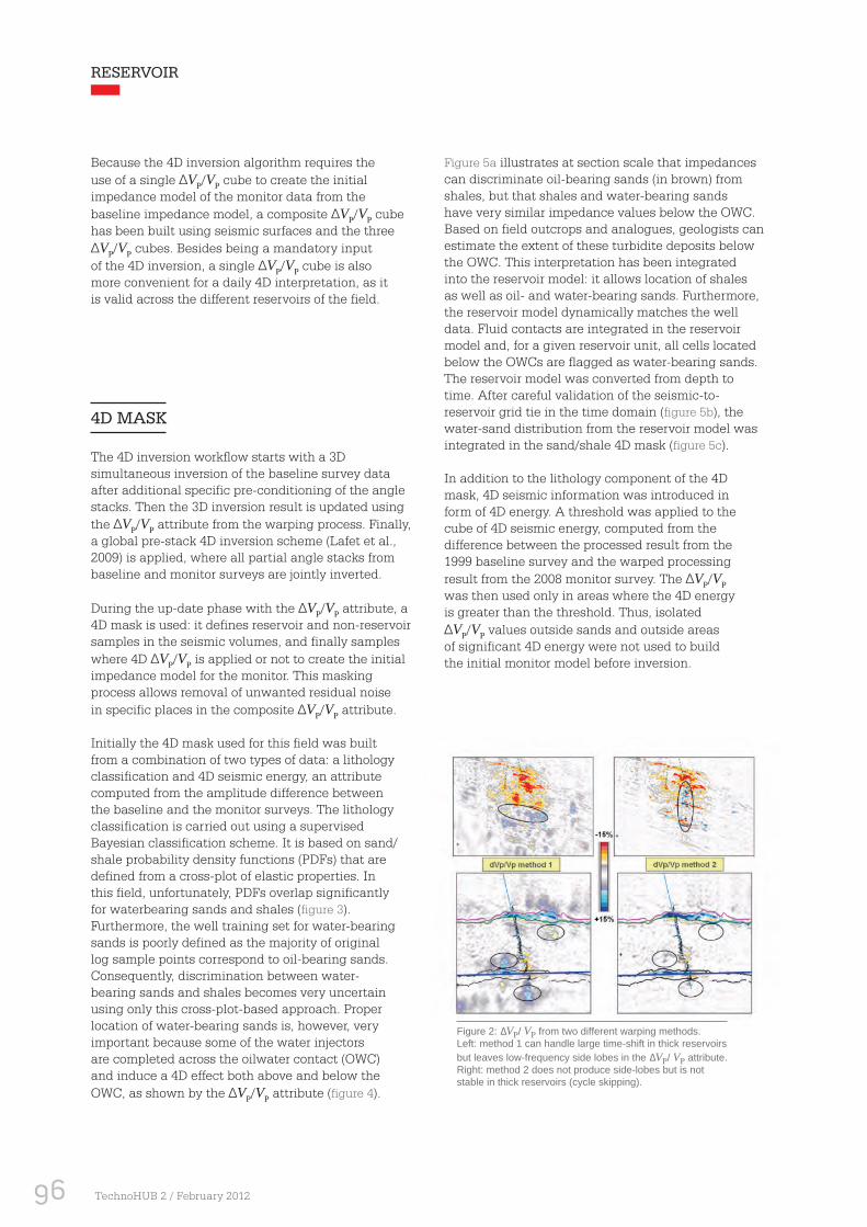
96 TechnoHUB 2 / February 2012
4D MASK
The 4D inversion workflow starts with a 3D simultaneous inversion of the baseline survey data after additional specific pre-conditioning of the angle stacks. Then the 3D inversion result is updated using the ∆VP/VP attribute from the warping process. Finally, a global pre-stack 4D inversion scheme (Lafet et al., 2009) is applied, where all partial angle stacks from baseline and monitor surveys are jointly inverted.
During the up-date phase with the ∆VP/VP attribute, a 4D mask is used: it defines reservoir and non-reservoir samples in the seismic volumes, and finally samples where 4D ∆VP/VP is applied or not to create the initial impedance model for the monitor. This masking process allows removal of unwanted residual noise in specific places in the composite ∆VP/VP attribute.
Initially the 4D mask used for this field was built from a combination of two types of data: a lithology classification and 4D seismic energy, an attribute computed from the amplitude difference between the baseline and the monitor surveys. The lithology classification is carried out using a supervised Bayesian classification scheme. It is based on sand/shale probability density functions (PDFs) that are defined from a cross-plot of elastic properties. In this field, unfortunately, PDFs overlap significantly for waterbearing sands and shales (figure 3). Furthermore, the well training set for water-bearing sands is poorly defined as the majority of original log sample points correspond to oil-bearing sands. Consequently, discrimination between water-bearing sands and shales becomes very uncertain using only this cross-plot-based approach. Proper location of water-bearing sands is, however, very important because some of the water injectors are completed across the oilwater contact (OWC) and induce a 4D effect both above and below the OWC, as shown by the ∆VP/VP attribute (figure 4).
Figure 2: ΔVP/ VP from two different warping methods. Left: method 1 can handle large time-shift in thick reservoirs but leaves low-frequency side lobes in the ΔVP/ VP attribute. Right: method 2 does not produce side-lobes but is not stable in thick reservoirs (cycle skipping).
Because the 4D inversion algorithm requires the use of a single ∆VP/VP cube to create the initial impedance model of the monitor data from the baseline impedance model, a composite ∆VP/VP cube has been built using seismic surfaces and the three ∆VP/VP cubes. Besides being a mandatory input of the 4D inversion, a single ∆VP/VP cube is also more convenient for a daily 4D interpretation, as it is valid across the different reservoirs of the field.
Figure 5a illustrates at section scale that impedances can discriminate oil-bearing sands (in brown) from shales, but that shales and water-bearing sands have very similar impedance values below the OWC. Based on field outcrops and analogues, geologists can estimate the extent of these turbidite deposits below the OWC. This interpretation has been integrated into the reservoir model: it allows location of shales as well as oil- and water-bearing sands. Furthermore, the reservoir model dynamically matches the well data. Fluid contacts are integrated in the reservoir model and, for a given reservoir unit, all cells located below the OWCs are flagged as water-bearing sands. The reservoir model was converted from depth to time. After careful validation of the seismic-to-reservoir grid tie in the time domain (figure 5b), the water-sand distribution from the reservoir model was integrated in the sand/shale 4D mask (figure 5c).
In addition to the lithology component of the 4D mask, 4D seismic information was introduced in form of 4D energy. A threshold was applied to the cube of 4D seismic energy, computed from the difference between the processed result from the 1999 baseline survey and the warped processing result from the 2008 monitor survey. The ∆VP/VP was then used only in areas where the 4D energy is greater than the threshold. Thus, isolated ∆VP/VP values outside sands and outside areas of significant 4D energy were not used to build the initial monitor model before inversion.
RESERVOIR

97February 2012 / TechnoHUB 2
Figure 3: A cross-plot of the detrended VP/VS ratio versus the relative P-impedance from the 3D baseline inversion. Water-bearing sands are not discriminated from shales in this cross-plot. To build the 4D mask, additional information is needed.
Figure 5: (a) Section through the impedance cube showing that water-bearing sands are not discriminated from shales. (b) Locations of water-bearing sands on the section are identifi ed from the reservoir model to improve the sandshale classifi cation for (c) the 4D mask that discriminates sands from shales.
4D CONSTRAINTS
The 4D global inversion applied in this study uses a CGG-Veritas proprietary algorithm that optimizes a multi-vintage cost function combining several terms. Time-lapse coupling of the inversion scheme is achieved by restricting the range of perturbations between successive surveys according to user-specified constraints. Specifically, between each consecutive vintage, perturbations are restricted to specific user-defined ranges of density and P-wave and S-wave velocity. In order to determine these intervals, reservoir simulations were performed at the initial reservoir state and at the time of the 4D seismic acquisition. The simulated parameters are the pressure and fluid saturations. The reservoir model also provides porosity and clay content parameters. Then, from a 4D rock-physics model and simulated reservoir parameters, the density and P-wave and S-wave velocities are computed (figure 6 p. 98) and therefore the relative density and P-wave and S-wave velocity variations between the initial state of the reservoir and the time of the 4D seismic acquisition can be computed. Final inverted impedance variations are limited by this a priori range of property variations.
Figure 4: A map of ΔVP/VP from the warping showing 4D anomalies due to injection above and below the OWC. ΔVP/VP is negative below the OWC, because of the much lower salinity of the injected water, compared to the formation water.

98 TechnoHUB 2 / February 2012
QUALITATIVE ANALYSIS OF THE 4D INVERSION RESULTS
One of the objectives of the 4D pre-stack inversion was to provide the best 4D images for interpreters, compared to previous attributes. An example close to a water-injector injecting into oil-bearing sands is presented in figure 7. Looking at the ∆VP/VP cube from the warping (figure 7b), 4D anomalies have a lower magnitude and some of them tend to go up in shaly levels. This is not in agreement with the knowledge of the field: due to gravitational segregation the injected water tends to go down in the reservoirs. Figure 7c shows a section through the cube of relative P-impedance change, ∆ IP/IP , between the baseline and monitor surveys. The anomalies have a stronger magnitude, more in line with the sand occurrence, and are no longer present in shales above the reservoir. Furthermore on the ∆VP/VP section, the first completed level (on the left of the image) exhibits a very weak anomaly. The injection efficiency could be doubtful with such an image. The 4D inversion shows a different signal compared to the ∆VP/VP section, and allows us to conclude that the uppermost completed level injects with good efficiency.
In order to transfer information from 4D seismic data into the reservoir model, 3D geobodies were picked on 4D seismic data and upscaled onto the reservoir grid, highlighting the reservoir model cells affected by depletion or by water saturation increase. Figure 8 compares geobodies picked on ∆VP/VP from warping and on ∆ IP/IP from the inversion. The section contains the trajectory of a producing well. The ∆VP/ VP section contains more side-lobes and lacks low frequency content, which makes the geobody discontinuous in the heart of the channel. The ∆ IP/IP section from the 4D inversion has smaller side-lobes and a more accurate geobody can be picked, so information of higher quality is transmitted to the reservoir engineers at the reservoir model scale.
Figure 6: Method to build the 4D constraints for the 4D inversion. Reservoir simulations provide properties at the time of the 4D and at the initial reservoir state. A rock-physics model is then applied to transform variation of reservoir properties into relative variations of elastic parameters.
Figure 7: (a) Part of a band-passed section through the P-impedance volume close to a water injector. (b) ∆VP/VP for the same section from the warping and (c) ∆ IP/IP for the section from the 4D inversion. ∆ IP/IP shows stronger and sharper 4D anomalies, more in agreement with sand occurrence, well correlated with (a).
RESERVOIR

99February 2012 / TechnoHUB 2
QUANTITATIVE ANALYSIS OF 4D INVERSION RESULTS
To make a more quantitative analysis, ∆VP/VP from the warping was cross-plotted versus ∆ IP/IP from the inversion (figure 9). Seismic samples were first selected in the vicinity of a water injector. As expected, ∆VP/VP and ∆ IP/IP are well correlated (~76%). More interestingly, a simple linear regression between ∆ IP/IP and ∆VP/VP shows that ∆VP/VP ≈ 0.78∆ IP/IP. The P-wave impedance, IP , is the product of the density, ρ, and VP. Because all parameters vary as a function of the 4D effects, we can write the following equation:
∆IP/IP = ∆ ρ/ρ + ∆VP/VP (1)
Figure 8: Comparison between ∆VP/VP (left) from the warping and ∆ IP/IP (middle) from the 4D inversion. In the vicinity of this oil producer, ∆ IP/IP has smaller sidelobes and is richer in low frequencies. This provides a more relevant geobody for the reservoir engineers (right).
From the ∆ IP/IP versus ∆VP/VP cross-plot, we know that ∆VP/VP ≈ 0.78∆ IP/IP , and an exploration of the ∆VP/VP volume shows values up to +20% close to water injectors. This information and Equation (1) yield ∆ ρ/ρ ≈ 0.06. Therefore, close to injectors, the 4D inversion shows a significant density effect, in line with expectation from the rock physics knowledge of this field. This quantitative result also explains the fact that images from the ∆ IP/IP cube show stronger, sharper anomalies and are easier to interpret than images from the ∆VP/VP cube close to the water injectors.The same type of quantitative analysis has been carried out close to the oil producers, where a few percent of exsolved gas should not affect the density significantly.
Figure 10 shows a cross-plot of ∆ IP/IP against ∆VP/VP built by selecting seismic samples in the vicinity of an oil producer. A high correlation of 85% was found. The cross-plot also shows that close to oil producers, ∆VP/VP ≈ 0.96∆ IP/IP. With Equation (1) and maximum values of 25% for ∆VP/VP , the calculated relative density change close to producers is ∆ ρ/ρ ≈ 0.01. In other words, the inversion values for ∆ IP/IP show negligible density effects close to the oil producers, in line with expectations. These results are very encouraging for a quantitative use of the ∆ IP/IP from the 4D inversion. It also shows that, quantitatively, both ∆ IP/IP from the 4D pre-stack inversion and ∆VP/VP from the warping are reliable because their relationships are in line with the expectations in the vicinity of the wells.
Figure 9: Top: ∆ IP/IP section close to a water injector. Bottom: cross-plot of ∆VP/ VP versus ∆ IP/IP for points extracted from the rectangular area marked on the section. Signifi cant density effects can be deduced from the cross-plot in the vicinity of water injectors.
Figure 10: Top: ∆ IP/IP section close to an oil producer. Bottom: cross-plot of ∆ VP/VP versus ∆ IP/IP for points extracted from the rectangular area marked on the section, showing negligible density effects in the vicinity of oil producers.

100 TechnoHUB 2 / February 2012
As the 4D inversion was pre-stack, it was also decided to investigate the relevance of ∆ IS/IS, the relative variations of the S-wave impedance between the baseline and the monitor seismic. A good location to carry out such an analysis is close to a gas injector: here the oil is partially substituted by the injected gas, which should induce a significant change in the density. Seismic samples were selected close to a gas injector, and ∆ IS/IS was cross-plotted versus ∆ IP/IP (figure 11). The cross-plot shows a high correlation coefficient of 83% with the linear regression between the two attributes being ∆ IS/IS ≈ 0.13∆ IP/IP.
We know that IS= ρVS= √μρ, where μ is the rigidity modulus. As ρ varies as a function of 4D effects, one can write:
∆ IS/IS = ∆ρ/2ρ (2)
The cross-plot of ∆ IS/IS versus ∆ IP/IP shows
Figure 11: Top and middle: ∆ IP/IP and ∆ IS/IS sections close to a gas injector. Bottom: cross-plot of ΔIS/ IS versus ∆ IP/IP for points extracted from the area outlined by the black dashed line on the section, showing signifi cant density effects in the vicinity of a gas injector.
Figure 12: Comparison between ∆ VP/VP and ∆ IP/IP in a tuning area. The cross-plot shows ∆ VP/VP versus ∆ IP/IP coloured by the time thickness of the interval. The model-based 4D inversion is less sensitive to tuning.
maximum values of 25% for ∆ IP/IP close to the gas injectors. With this value, Equation (2), and the relationship ∆ IS/IS ≈ 0.13∆ IP/IP, one can deduce that close to the gas injector there is a significant density effect of about 7%. This effect is in line with expectations, and shows the relevance of the two attributes, ∆ IP/IP and ∆VP/VP provided by the 4D inversion, at least close to the gas injectors.
As discussed earlier, the reservoirs in this field comprise unconfined thin deposits and of thicker confined deposits. Deposits thinner than 7 m are affected by the tuning. It was decided to compare the ∆VP/VP attribute from the warping to the ∆ IP/IP attribute from the 4D inversion to evaluate the effect of tuning close to an oil producer (figure 12).
RESERVOIR

101February 2012 / TechnoHUB 2
ConclusionsAn innovative 4D pre-stack inversion workflow was developed. The specific properties of the field required the development and application of new Total in-house warping techniques. The large 4D signal magnitude variations between the different depositional systems in the field caused there to be no global stable warping solution. As the 4D inversion workflow required a single ∆VP/VP cube, a composite ∆VP/VP cube was built from the elementary warping cubes using seismic horizons. The 4D pre-stack inversion workflow integrates not only seismic information but also well information, used to discriminate sand from shale during the 4D mask building, as well as a 4D rock-physics model. Moreover, because water-bearing sands are hard to discriminate from shales in some reservoirs in the field, information from the reservoir grid was also introduced in the process in order to locate the water-bearing sands in the mask.
Qualitative analysis of the 4D pre-stack inversion results has shown an improvement compared to other 4D seismic attributes: sharper images and better quality information, in particular close to water injectors, allowing better 3D geobody picking around the 4D anomalies. Quantitative analysis of the 4D inversion results has also shown that the relative numerical values of the ∆ IP/IP and ∆VP/ VP attributes are reliable: significant density effects are shown by the inversion close to the water or gas injectors. Furthermore, the inversion does not show significant density effects close to the oil producers, where the ∆VP/VP attributes largely dominates the resulting ∆ IP/IP, a result in line with expectations with knowledge of the field. As the 4D inversion was prestack, not only ∆ IP/IP but also ∆ IS/IS has been investigated and has proven to be relevant, at least close to the gas injectors. Another positive impact of the 4D inversion is its detuning effect. It allows more confident 4D seismic interpretation in thin deposits.
The 4D inversion has reached its objectives: providing the most relevant set of 4D seismic attributes, complementary to the already existing attributes such as amplitude differences and ∆VP/VP from the warping. Besides the operational impact, the quantitative analysis shows the relevance of the inversion attributes and has opened the way to a more quantitative use, yet to be investigated. Once again, 4D seismic surveying turns out to be a key monitoring technique to improve hydrocarbon recovery, which is a strategic axis for our exploration and production, particularly in the challenging but rewarding deep offshore environment.
ACKNOWLEDGEMENTS Total thanks the block concessionaire, Sonangol and its partners Statoil Angola Block 17, Esso Exploration Angola, and BP for permission to publish this work.
REFERENCES
Lafet, Y., Roure, B., Doyen, P.M. and Buran, H. [2009] Global 4-D seismic inversion and time-lapse fl uid classifi cation. 79th SEG Annual Meeting, Expanded Abstracts, 28, 3830–3834.
Lumley, D., Adams, D., Meadows, M., Cole, S. and Ergas, R. [2003] 4D Seismic pressure-saturation inversion at Gullfaks fi eld, Norway. First Break, 21(9), 49–58.
McInally, A., Kunka, J., Garnham, J., Redondo-Lopez, T. and Stenstrup- Hansen, L. [2001] Tracking production changes in a turbidite reservoir using 4D elastic inversion. 63rd EAGE Conference & Exhibition, Extended Abstracts, P665.
Rutledal, H., Helgesen, J. and Buran, H. [2003] 4D elastic inversion helps locate in-fi ll wells at Oseberg fi eld. First Break, 21(8), 43–48.
Williamson, P.R., Cherrett, A.J. and Sexton, P.A. [2007] A new approach to warping for quantitative time–lapse characterisation. 72nd EAGE Conference & Exhibition, Extended Abstracts, P064.
Received 27 January 2011; accepted 23 June 2011. doi: 10.3997/1365-2397.2011024
At map scale and at section scale, the comparison shows ∆ IP/IP anomalies of higher magnitude and larger extent. The ∆ IP/IP attribute seems less impacted by the tuning in the thin spill deposits, indicated by the arrows. In order to have a more quantitative insight, ∆VP/VP vales were cross-plotted versus the ∆ IP/IP and the points from the two maps were coloured by the time thickness of the reservoir. This cross-plot shows that the ∆VP/VP attribute is systematically smaller than the ∆ IP/IP and that the difference increases as the
time-thickness decreases. Again this is consistent with theoretical considerations: the warping being a completely data-driven process has an upper bandwidth limit set by the high end of the seismic frequency spectrum. In the 4D inversion, however, high-frequency information is obtained through the use of a stratigraphic grid in a model-based inversion process. Therefore, the 4D inversion is less sensitive to the tuning and turns out to be a more relevant tool for 4D interpretation in tuning areas.

102 TechnoHUB 2 / February 2012
DRILLING & WELLS
The ongoing search for new resources naturally leads to exploring and developing deeper and deeper reservoirs. Since achieving depths of 5,000 m in the 1960s, the industry has progressed, such that it is not unusual to see wells of more than 6,500 m today. This increase in burial depth comes with rising pressure and temperature levels, calling for the development of new technologies and materials to meet the needs of exploring and producing these reservoirs in extreme conditions.
Infill drilling know-how is crucial in this context, as it limits the pre-investment phase. During the subsequent production phase, more infill wells are also drilled to replace lost wells and increase the amount and rate of recovery.
On the Elgin and Franklin fields, advanced drilling methods were developed to overcome the high depletion (100 bar every 6 months initially) that paradoxically, has made infill wells more difficult to drill than initial development wells. Intense engineering work has been carried out
to better understand the impact of depletion on compaction and the fracture gradient; design and qualify new drilling mud systems combined with stress caging techniques; and prepare contingent solutions with the deployment of expandable - and drilling - liner technologies.
To date, Total has successfully drilled, completed and brought several infill wells into production in the Elgin and Franklin fields on the UKCS (United Kingdom Continental Shelf). This has been achieved in severely depleted reservoirs - more than 800 bar - and has opened the door for phased HP/HT developments and deep exploration beneath depleted horizons.
Over the past 50 years, through the development of the Lacq field and its satellites, Total has fine-tuned its know-how in HP/HT, onshore as well as offshore, on fixed installations. However, more challenges still lie ahead, such as HP/HT in deep water (Azerbaijan, Egypt); the aging of HP/HT fields in production (UK) and ever-higher temperatures (Malaysia).
CONTEXT

103February 2012 / TechnoHUB 2
Advanced Drilling in HP/HT: The TOTAL Experience on Elgin/Franklin (North Sea – UK)
Drilling HP/HT exploration wells remains a challenge despite years of experience acquired by the Drilling & Completion industry. Development wells have further pulled the envelope of performance of the technologies and procedures required to safely and economically deliver the production from the HP/HT fields. Now comes the time of drilling and completing infill wells, which paradoxically appear more difficult as depletion increases and mud weight window disappears.
To overcome this hurdle, intense engineering works have been carried out to better understand the impact of the depletion on compaction and fracturing gradient, to design and qualify new drilling mud systems combined with stress caging techniques and to prepare contingent solutions with the deployment of expandable and drilling liner technologies.
As of today three infill wells have been successfully drilled, completed and put in production by Total in the Elgin/Franklin fields on the United Kingdom Continental Shelf (UKCS). This has been achieved, through severely depleted reservoirs−with more than 800 bars depletion−and has opened the door for phased HP/HT developments and deep exploration beneath depleted horizons.
by Jean-Louis BERGEROT, Total
EXTRACTJournal of Petroleum TechnologyOctober 2011
ABSTRACT

104 TechnoHUB 2 / February 2012
OVERVIEW OF THE ELGIN/FRANKLIN EXTREME HP/HT FIELDS
The Elgin/Franklin fields present an extreme combination of pressure and temperature in the world (1,100 bar virgin pressure and 200°C) and remains today the largest HP/HT gas condensate field developed in the British Sector of the North Sea. The fields lie approximately 200 km Northeast of Aberdeen in the Central Graben area.
Following the discovery and appraisal period from 1985 to 1994, the development started in 1996 with two unmanned wellhead platforms tied back to a central production facility. Eleven wells were drilled and put on stream, with deviation up to 50°, for an average drilling duration of 120 days. These wells were all drilled before a pre defined limit of depletion level has been reached, level at which the mud weight window closes calculated on Elgin/Franklin as being 100 bars. First oil took place in 2001. Later, two satellite structures, Glenelg and West Franklin have been drilled and put in production via the existing installations, respectively in 2006 and 2007 (figure 1).
The reservoirs consist of Jurassic sandstones deeply buried at a depth exceeding 5,300 m. The primary reservoir is the Fulmar also called Franklin sands. Reservoir fluids are gas condensate with a bottomhole pressure of 1,100 bar and temperature of 190°C. The Fulmar reservoir is underlain by the Pentland reservoir with bottomhole conditions of 1,150 bar and temperatures of 200°C (figure 2).
Despite the great depth, the main reservoir shows significant porosity and permeability, allowing strong productivity. Up to 30% porosity and 1D permeability are seen in some Fulmar layers.
The individual wells on the field can produce up to a maximum gas rate of 3.5×10⁶ m3/d gas with associated condensate. Production will give surface conditions of 860 bar wellhead shut in pressure with an associated surface temperature of 180°C. In the produced effluent, 3 to 4% CO2 and 30-40 ppm H2S are present. Initially, field gas production reached 14.6×10⁶m3/d, with 24,000 m3/d (or 150,000 BOEPD) of condensate.
This combination explains the strong need of technology and in depth engineering for these wells.
CHALLENGES OF INFILL WELLS
Infill wells may be needed for various reasons. As for conventional field management, they may be used to increase the recovery factor, hence the reserves produced, or to accelerate the delivery or to improve the drainage.
In addition they may be required to replace wells which have failed. On HP/HT fields like Elgin/Franklin, wells are exposed to multiple threats due to the large amount of depletion that they will see.
One such threat is sand or solids production which can lead to erosion of equipment such as the downhole safety valve, tree, or surface production piping. Rock mechanics studies suggest that sand production is inevitable beyond certain depletion.
Currently, no field proven downhole sand control method can be implemented in the more severe HP/HT wells. Should such event occur, wells will have to be choked down and can ultimately be lost, which leads to a significant production loss.
Another threat is the liner deformation because of the compaction triggering the buckling of the liner, or because of tectonic movements along faults or other bedding planes. At the end the liner may even be fully sheared off.
Figure 1: Central Graben development.
DRILLING & WELLS
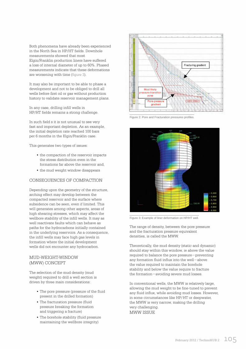
105February 2012 / TechnoHUB 2
Figure 2: Pore and Fracturation pressures profi les.
Both phenomena have already been experienced in the North Sea in HP/HT fields. Downhole measurements showed that most Elgin/Franklin production liners have suffered a loss of internal diameter of up to 60%. Phased measurements indicate that these deformations are worsening with time (figure 3).
It may also be important to be able to phase a development and not to be obliged to drill all wells before first oil or gas without production history to validate reservoir management plans.
In any case, drilling infill wells in HP/HT fields remains a strong challenge.
In such field s it is not unusual to see very fast and important depletion. As an example, the initial depletion rate reached 100 bars per 6 months in the Elgin/Franklin case.
This generates two types of issues:
▪ the compaction of the reservoir impacts the stress distribution even in the formations far above the reservoir and,
▪ the mud weight window disappears CONSEQUENCES OF COMPACTION
Depending upon the geometry of the structure, arching effect may develop between the compacted reservoir and the surface where subsidence can be seen, even if limited. This will generates among other aspects, areas of high shearing stresses, which may affect the wellbore stability of the infill wells. It may as well reactivate faults which can behave as paths for the hydrocarbons initially contained in the underlying reservoirs. As a consequence, the infill wells may face high gas levels in formation where the initial development wells did not encounter any hydrocarbon.
MUD-WEIGHT-WINDOW (MWW) CONCEPT
The selection of the mud density (mud weight) required to drill a well section is driven by three main considerations:
▪ The pore pressure (pressure of the fluid present in the drilled formation)
▪ The fracturation pressure (fluid pressure breaking the formation and triggering a fracture)
▪ The borehole stability (fluid pressure maintaining the wellbore integrity)
The range of density, between the pore pressure and the fracturation pressure equivalent densities, is called the MWW.
Theoretically, the mud density (static and dynamic) should stay within this window, ie above the value required to balance the pore pressure−preventing any formation fluid influx into the well−above the value required to maintain the borehole stability and below the value require to fracture the formation−avoiding severe mud losses.
In conventional wells, the MWW is relatively large, allowing the mud weight to be fine-tuned to prevent any fluid influx, while avoiding mud losses. However, in some circumstances like HP/ HT or deepwater, the MWW is very narrow, making the drilling very challenging.MWW ISSUE
Figure 3: Example of liner deformation on HP/HT well.

106 TechnoHUB 2 / February 2012
For wells drilled before depletion, a mud weight window exists between the pore pressure and the fracturation pressure. When depletion occurs the fracturation pressure in the reservoir decreases along with the pore pressure. At the interface between the caprock, which stays at virgin pressure and the depleted reservoir, the MWW decreases to end up by not existing anymore (figure 4).
According to your well configuration, differentially depleted layers will have to be drilled in the same section, with a high risk of kick and losses or a combination of shales and depleted layers will be seen with the high risk of instability and losses. In any case, drilling becomes complex, difficult and the probability of occurrence of a failure increases with the depletion.
Ultimately, drilling with conventional techniques, within the fracturation gradient, is not possible anymore and new design, techniques and procedures have to be implemented.
On Elgin/Franklin, Rock Mechanics studies estimated the depletion limit to 100 bars. Until such time that the depletion was less than 100 bars, initial development well design was fit. Beyond, questions came of the use of additional strings, with the uncertainties on the right setting depth, of the feasibility of drilling above the fracturation gradient by reinforcing artificially the wellbore.
STATE OF THE ART OF THE HP/HT INFILL DRILLING
At the time of the evaluation of the feasibility of a first infill well on Elgin/Franklin, very few trials of HP/HT infill drilling were successfully achieved, and certainly none with a depletion level in excess of 600 bars. One HP/HT Operator faced severe losses problems when drilling through a formation depleted by 140 bars leading to the abandonment of the bottom of the well. Another HP/HT Operator did not manage to get to the final depth of an infill well because of too-low formation strength due to the depletion, preventing a safe drilling of the reservoir section.
Drilling through a 600 bar depleted reservoir in an HP/HT filed was clearly seen as far beyond what the Industry had achieved at that date. However, driven by the need of infill wells and
consequently of overcoming this depletion barrier, a feasibility study was launched which concluded that drilling such wells was feasible on the Elgin/Franklin fields and identified two possible well architectures. Based on these results, the development phase was launched and a target was selected on the Franklin field.
Figure 4: Mud-weight window disappears with depletion.
INFILL-WELL-DRILLING FEASIBILITY
UNCERTAINTIES IDENTIFICATION
The Fulmar reservoir consists of three main units:
▪ The C sands at the top have relatively poor characteristics: degraded permeability and presence of vertical baffles.
▪ The B sands in the middle have the best properties and are the main contributors to production.
▪ The A sands at the bottom are tighter, but can include good layers at the top.
Under the main Fulmar reservoir are the Pentland sands with poor characteristics. They are barely depleted and remain close to virgin pressure.
DRILLING & WELLS

107February 2012 / TechnoHUB 2
GEOMECHANICAL UNCERTAINTIES
Rock mechanic experts were brought in to estimate the two main rock properties necessary to design the well: fracture gradient of the reservoirs and borehole stability of the cap rock. The fracture-propagation gradient (FPG) is close to the minimum horizontal stress and can be modeled. In the case of Elgin/Franklin, a full scale rock mechanic model, coupled with the geological and dynamic reservoir model, had already been built and was used for this purpose. It estimated the FPG at 1.65-SG equivalent mud weight (EMW).
The fracture initiation gradient (FIG) is much more difficult than the FPG to predict, therefore, it was used only as an indication and considered as an uncertain, but existing, margin. On this well it was predicted to be around 1.87 SG EMW.
Both gradients are function of formation pressure. As such their profile suffers from the same uncertainty as the reservoir pressure profiles.
The other information requested from rock mechanics was the borehole stability of the cap rock. This allows definition of the minimum mud weight one can use to cross the transition zone without suffering unmanageable borehole instability of the open hole above. The amount of information on the cap rock is even more limited than on the reservoir.
GEOLOGICAL UNCERTAINTIES
Depending on the architecture selected, the top reservoir depth prediction was critical to maximize the success of the transition zone drilling. Extensive geophysical techniques were used to minimize the uncertainty attached to this test prediction. These included, among others, thorough examination of the seismic data and uncertainty studies on depth conversion. The prediction was given to +30 m and -45 m.
On Elgin/Franklin some thin limestone layers (centimetric to decimetric) are often found gas bearing in the cap rock. They can be drilled underbalanced but sometimes require high mud weight to enable trips.
RESERVOIR UNCERTAINTIES: DEFINING THE PORE PRESSURE PROFILE
The monitoring of the average pressure of existing Franklin producers had shown a depletion of more than 600 bar of the main reservoir. The pressure of the Fulmar B sands was confidently estimated at 500 bar at the planned reservoir penetration date. The pressure of the tighter C sands was more difficult to predict.
The highest uncertainty lies in the pressure transition profile between the cap rock, believed to have remained at virgin pressure, and the reservoir section. Is it at the very top of the reservoir or is the bottom of the cap rock affected by depletion through microfractures? How thick is the transition zone, and how steep is the pressure gradient in this zone?
Considering all uncertainties, different scenari were envisaged. A pressure profile along the well path was drawn and a probability of encountering higher pressure at top reservoir was evaluated for each scenario.
RETAINED WELL ARCHITECTURES
To tackle the drilling challenges described above, two different architectures were defined. The first one involves the use of a specially designed mud loaded preventively with specific lost-circulation materials (LCM). The technique is known as “borehole strengthening”. Once reservoir has been penetrated, the transition zone is cased off by a 7-in. liner.
The second one involves the use of an expandable liner to cover most of the cap rock. The transition zone is then drilled with a lower mud weight below the FPG. The remaining opened cap rock would be short enough so that borehole instabilities can be managed. The transition zone is then covered with a cemented 65/8-in. drilling liner. Once reservoir has been drilled, the 65/8-in. liner is covered by a 41/2-in. liner. Once transition zone is covered, the mud weight can be decreased to a value just enough to safely drill the reservoir.
As the main difficulty was lying across the transition zone crossing, the top architecture of the well was taken as a standard Elgin/Franklin architecture as designed for virgin pressure. This allowed focus on the transition zone crossing and gave a comfort factor, because this top architecture is designed to hold well full of gas at virgin reservoir pressure, regardless of circumstances.
BOREHOLE STRENGTHENING− HOW DOES IT WORK?
The borehole strengthening technique was already used in the industry. The principle is to create a fracture by using a mud weight higher than the FIP and plug it on creation, to prevent its further development. The plug is formed by loss circulation material (LCM) continuously present in the mud. The created fracture increases the rock stress locally, enhancing the hole’s ability to support high mud weight. It is more commonly used with water based mud which exhibit high filtration values.

108 TechnoHUB 2 / February 2012
The high temperatures experienced on Elgin/Franklin dictate the use of oil-based mud. As filtration of oil-based mud is very tight, the filtration from the fracture faces into the formation is virtually nil. The consequence is that the plug at the fracture mouth needs to be tightly sealing as soon as it is created.
The other difficulty is to define the width of the fracture to seal. Rock mechanics calculations show that there is a direct relationship between geometry of the fracture, width and length, and the amount of overpressure. The higher the pressure, the wider the fracture, at a given length. In our case, it was estimated that the mud could be designed to form an efficient plug of 1 mm width, while keeping reasonable rheological properties despite a high solid content.
The mud was therefore designed and tested to be able to seal a 1 mm gap. The LCM additives consist of sized grounded marble and sized graphitic material. Laboratory testing took place to adjust LCM additives relative concentrations, to achieve a quick and efficient plugging of 1mm slots. As well as these in house tests, tests were performed in a third-party laboratory.
MECHANICAL BACK-UP− HIGH-COLLAPSE EXPANDABLE AND DRILLING LINERS
Expandable liners are now becoming widely used in the industry to seal off weak zones to allow for increasing the mud weight to penetrate deeper zones at higher pressure. This makes them work under a burst mode. In our case, the expandable liner had to work in a collapse mode. Expanded pipe has low collapse capacity and this is one of the limitations of the technique. To increase the collapse capacity to the required value close to 350 bar, a development program was undertaken with the selected provider.
Although expandable liner has been run previously in high temperature wells, the operator thought it prudent to test the expansion system with high mud weight and high temperatures. This was done in a shallow well in a special facility in Dallas. The system was left soaking with 2.15 SG oil based mud at 176°C for 18 hours before initiating expansion and expanding 18 m of pipe. Examination of the seals and parts of the system afterwards showed no significant degradation. The system was declared qualified for the application.
The liner drilling technique was also becoming available at the time development work was ongoing. This technique presented two main advantages: firstly there is no need to trip out of hole to run the liner leaving the cap rock in an under balance condition for a long time. Secondly, it allows using a higher mud weight during drilling. If heavy losses were experienced when entering the reservoir, and the hydrostatic applied on the cap rock dropped, the formation may collapse. With a drilled in liner, it would collapse around the liner, leaving the hole cased off. Isolation behind the liner might be already achieved by the collapsed formation.
IMPLEMENTATION
Top sections were drilled as planned. The 133/8- in. casing was called 100 m short at 3,585 m. This resulted in a LOT (leak off test) value of 1.84-SG EMW instead of a planned 2.10-SG EMW. As drilling was progressing in the Herring formation, 150 m before planned phase total depth (TD) and 450 m above top reservoir, the gas level suddenly increased. The hole was stopped, and the production casing was run and successfully cemented at 4,939 m.
The main consequence of this event was that this Herring high-pressure layer was now to be crossed in the 8 ½ -in. section. Its required mud weight, confirmed when crossing it again, to be 2.05 SG minimum, was considered too high to implement the borehole strengthening technique. Therefore, the primary architecture was ruled out from the start of the 81/2- in. section. A decision was taken to implement the contingent architecture.
RUNNING EXPANDABLE LINER
Prior to run the liner, a caliper was run in the open hole to estimate the best placement for the elastomer bonded pipes. The hole proved to be mostly in gauge. The liner reached TD without any problem. The dart was dropped; The expansion process was initiated at a much higher pressure than expected, close to the burst pressure of the cone launcher element. Once initiated, the expansion process went smoothly and the liner was installed as planned.
DRILLING WITH LINER
Once the expandable shoe was cleared, and the stability of the well assessed, the 65/8 -in. drilled in liner was run. The well was displaced to the specially designed mud loaded with LCM originally designed for the borehole strengthening technique.
DRILLING & WELLS

109February 2012 / TechnoHUB 2
ConclusionsThe first infill well was successfully drilled, completed and perforated in an HP/HT reservoir after depletion of 660 bar had occurred.
Two different architectures were designed to achieve this goal and all contingencies have been used.
Despite a large amount of work performed to reduce geological and reservoir uncertainties, surprises were found. The biggest surprises were found in the overburden, long before reaching the reservoir. Most of them are believed to be a consequence of the reservoir depletion.
High permeability sands up to 100 md were drilled with 660 bar overbalance without any significant losses. The formation damage created by the designer mud, if any, was by-passed by the perforations.
This success has opened new perspectives in the HP/HT domain:
▪ It has permitted the development of additional reserves in the Elgin/Franklin reservoir. Two additional wells have now been successfully drilled through even more severely depleted reservoirs, close to 800 bar depletion.
▪ It gave assurance that wells that fail in future can be replaced, thus securing production over the life of field.
▪ On a wider perspective, phased HP/HT field developments can be contemplated. This will impact HP/HT field economics by allowing a reduction in pre-investments.
Nevertheless, HP/HT deep infill wells are not and will never be a routine job. Dedicated and integrated HP/HT teams (drilling, geologist, and others) combined with while drilling reactivity are key to success.
ACKNOWLEDGEMENTS The Elgin/Franklin fi elds are operated by Elf Exploration UKLtd on behalf of itself and of its coventurers: E.F. Oil and Gas Ltd * Eni Elgin/Franklin Ltd BG International (CNS) Ltd Ruhrgas UK Exploration & Production Ltd Esso Exploration and Production U.K. Ltd Texaco Britain Ltd Dyas UK Ltd Oranje-Nassau (U.K.) Ltd
*E.F. Oil and Gas Ltd, a company in which the shares are held 77.5% by Elf Exploration UK Ltd and 22.5% by Gaz de France
The liner drilled the remaining of the cap rock and penetrated the reservoir at 5,451 m. No more than 500 liters of losses were noticed when penetrating the reservoir. These very low levels of losses lead to questioning the top reservoir depletion. Drilling was continued until 5,484 m where the liner hanger was about to hang on top of the expandable liner. The liner was then cemented.
RESERVOIR DRILLING
Having achieved the successful isolation of the transition between cap rock and reservoir, one could believe that the mud weight could be decreased to drill the remaining of the reservoir with a minimum overbalance.
Mud weight was decreased down to 1.50 SG prior to drilling the shoe. High levels of gas were experienced as soon as the shoe was drilled. Mud weight was raised to 1.60 SG and drilling continued on 40 m, in the believed poor productivity C sands, with still high gas levels. The well was displaced back to 1.86 SG designer mud to allow a safe trip out of hole.
Well logs showed the presence of good sands at the top of the reservoir, covered only partially by the drilled in liner, pressurized up to 1,004 bar, forbidding to lower the mud weight.
The only remaining option was to drill to final depth with the designer mud. The losses response plan was updated accordingly, and drilling continued at a reduced penetration rate into the remaining C sands, the B sands and 55 m into the A sands. TD was reached at 5,678 m with only a seepage losses rate noticed around 200 liters/hour for a small period. It is difficult to ascertain which of the following happened:
▪ The borehole was fractured and the borehole strengthening technique worked, or
▪ The designer mud increased the fracture initiation pressure by creating a perfect seal between the borehole and the formation, or
▪ The mud column pressure was below the initial fracture initiation pressure.
Final 41/2-in. liner was then run, and the well has been completed, perforated and put on stream at an initial 17,000 B/D.

110 TechnoHUB 2 / February 2012
FIELD OPERATIONS
More and more oil and gas developments are located offshore. Nevertheless, with easily accessible oil and gas provinces already having been explored, future developments will take place in increasingly harsh environments, such as the west of Shetlands North Sea, deeper and deeper offshore as well as ice-covered arctic waters.
The current focus is on innovation in techniques and materials that enable human access to those ever-more difficult targets. A prime example is the Swimmer system for which Cybernetix, Statoil and Total initiated a feasibility study in 2007. After 18 months, Total decided to study further the Swimmer concept for the offshore Angolan specific application.
Swimmer is a vehicle that performs inspection, maintenance and repair of subsea production systems with enhanced versatility and responsiveness. It is a hybrid system composed of an AUV (Autonomous Underwater Vehicle) and a ROV (Remotely Operated Vehicle).
As such, it can perform pipeline inspections in AUV mode and light interventions on subsea equipment by deploying its own embedded ROV operated from topside production facilities.
This innovative vehicle is designed to reduce operational risks as well as operating costs as it does not call anymore for a ROV support vessels. It is engineered to remain on the seafloor for up to three months at a time, without any need for maintenance.
Swimmer is undergoing further development to meet tomorrow’s challenges – including deployment in arctic regions.
CONTEXT

111February 2012 / TechnoHUB 2
Subsea intervention system for arctic and harsh weatherAlain FIDANI, Gabriel GRENON - CybernetixEric RAMBALDI, Nicolas TITO - TotalErich LUZI – Statoil
Swimmer is a new hybrid AUV/ROV subsea intervention system for light inspection, maintenance, and repair (IMR) operations on subsea production systems (SPS). One prime advantage is that it can carry out IMR operations on its own, without a field support vessel. Once the Swimmer AUV shuttle is resting on its docking station, the ROV can be controlled fully from surface facilities via the production control umbilical. The Swimmer’s technical feasibility was shown in 2001 by full-scale sea trials. Since 2007, Total, Statoil, and Cybernetix have cooperated to develop a commercial version.
Although the first application of this technology is earmarked for Total’s Angola block 17 in late 2011, the partners are investigating use of the Swimmer system in offshore fields with extreme weather conditions.
Swimmer not only can boost the flexibility and reduce the cost of operations for deep offshore fields, but also may become an enabling technology on ice-covered arctic fields or in harsh environments such as the North Sea. The weather at these fields can prevent intervention vessels from operating for long periods, and is a personnel safety concern. In these conditions, the Swimmer’s ability to remain deployed subsea for several consecutive weeks is a key point for the operability and maintenance of such fields.
For arctic regions, operations during ice formation and ice thickness may require an expensive icebreaker vessel. Drifting icebergs also threaten support vessels and production facilities. Sea state for some harsh environment areas may exceed Level 7 during parts of the year, making deployment and recovery of subsea intervention vehicles dangerous.
Swimmer can be a tool to operate and or maintain subsea production assets when infrastructure is not reachable from the surface.
EXTRACTOff shoreFebruary 2010
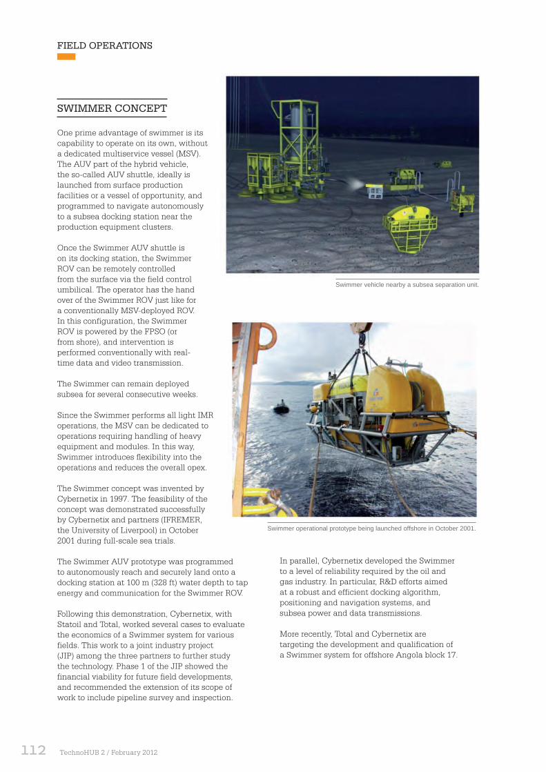
112 TechnoHUB 2 / February 2012
SWIMMER CONCEPT
One prime advantage of swimmer is its capability to operate on its own, without a dedicated multiservice vessel (MSV). The AUV part of the hybrid vehicle, the so-called AUV shuttle, ideally is launched from surface production facilities or a vessel of opportunity, and programmed to navigate autonomously to a subsea docking station near the production equipment clusters.
Once the Swimmer AUV shuttle is on its docking station, the Swimmer ROV can be remotely controlled from the surface via the field control umbilical. The operator has the hand over of the Swimmer ROV just like for a conventionally MSV-deployed ROV. In this configuration, the Swimmer ROV is powered by the FPSO (or from shore), and intervention is performed conventionally with real-time data and video transmission.
The Swimmer can remain deployed subsea for several consecutive weeks.
Since the Swimmer performs all light IMR operations, the MSV can be dedicated to operations requiring handling of heavy equipment and modules. In this way, Swimmer introduces flexibility into the operations and reduces the overall opex.
The Swimmer concept was invented by Cybernetix in 1997. The feasibility of the concept was demonstrated successfully by Cybernetix and partners (IFREMER, the University of Liverpool) in October 2001 during full-scale sea trials.
The Swimmer AUV prototype was programmed to autonomously reach and securely land onto a docking station at 100 m (328 ft) water depth to tap energy and communication for the Swimmer ROV.
Following this demonstration, Cybernetix, with Statoil and Total, worked several cases to evaluate the economics of a Swimmer system for various fields. This work to a joint industry project (JIP) among the three partners to further study the technology. Phase 1 of the JIP showed the financial viability for future field developments, and recommended the extension of its scope of work to include pipeline survey and inspection.
In parallel, Cybernetix developed the Swimmer to a level of reliability required by the oil and gas industry. In particular, R&D efforts aimed at a robust and efficient docking algorithm, positioning and navigation systems, and subsea power and data transmissions.
More recently, Total and Cybernetix are targeting the development and qualification of a Swimmer system for offshore Angola block 17.
Swimmer vehicle nearby a subsea separation unit.
Swimmer operational prototype being launched offshore in October 2001.
FIELD OPERATIONS

113February 2012 / TechnoHUB 2
MAIN FEATURES
The Swimmer system is composed of both fixed and mobile assets. The fixed assets are part of the offshore field infrastructures and include the following:
▪ Subsea docking stations
▪ Subsea power and data cables embedded into the field control umbilical
▪ Control consoles integrated into the FPSO control room.
The hybrid vehicle and the associated IMR tools form the mobile assets and include the following:
▪ AUV shuttle
▪ Light Work-ROV equipped with two manipulator arms
▪ Work-ROV TMS integrated into the AUV shuttle
▪ ROV tools for light IMR operations.
The Swimmer is designed to stay deployed subsea for up to three months. The current design depth is 1,500 m (4,921 ft) but can be extended to 3,000 m (9,842 ft). The AUV shuttle operating range is 20 km (12 mi) in the standard configuration, but can be extended to 50 km (31 mi), and cruising speed is up to 2 knots. Once docked, the ROV excursion around the docking station is in the 200 m (656 ft) range.
The IMR tasks that can be performed by the Swimmer ROV include the following:
1. Valve operation
2. Cleaning
3. Global, close, and detailed visual inspection
4. Wall thickness measurement
5. Cathodic protection measurement
6. Support to electrical diagnosis and trouble shooting /fault finding
7. Assistance to large module replacement
8. Disconnection of lying leads
9. Fluid and thermal leak detection
Swimmer AUV shuttle landing on docking station.
Swimmer light WROV leaving shuttle.
10. Subsea sampling
11. Replacement of small components
12. Any other ROV operation requiring only the use of manipulators or manipulator carried tools.
The Swimmer AUV can be programmed for field survey and pipeline inspection tasks such as the following:
1. Field mapping
2. Pipeline survey
3. Pipeline close visual inspection
4. Pipeline free span detection
5. Pipeline localization
6. Dropped objects detection
7. Cathodic protection measurement. The hybrid Swimmer vehicle combines ROV-borne IMR capabilities, suitable for maintaining SPS within tether range from the docking stations, with AUV-borne inspection capabilities for survey and inspection of subsea flowlines. Together, the scope of tasks covers the needs for all light IMR operations necessary to maintain a facility in production except replacement of large modules.
The tools for IMR tasks on an SPS are generally small and can be embarked directly by the light Work-ROV, or alternatively put into storage compartments onboard the AUV shuttle.
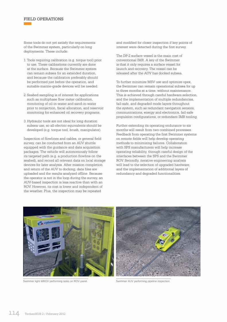
114 TechnoHUB 2 / February 2012
Some tools do not yet satisfy the requirements of the Swimmer system, particularly on long deployments. These include:
1. Tools requiring calibration (e.g. torque tool) prior to use. These calibrations currently are done at the surface. Because the Swimmer system can remain subsea for an extended duration, and because the calibration preferably should be performed just before the operation, and suitable marine-grade devices will be needed.
2. Seabed sampling is of interest for applications such as multiphase flow meter calibration, monitoring of oil-in-water and sand-in-water prior to reinjection, fiscal allocation, and reservoir monitoring for enhanced oil recovery programs.
3. Hydraulic tools are not ideal for long duration subsea use, so all-electric equivalents should be developed (e.g. torque tool, brush, manipulator).
Inspection of flowlines and cables, or general field survey, can be conducted from an AUV shuttle equipped with the guidance and data acquisition packages. The vehicle will autonomously follow its targeted path (e.g. a production flowline on the seabed), and record all relevant data on local storage devices for later analysis. After mission completion and return of the AUV to docking, data files are uploaded and the results analyzed offline. Because the operator is not in the loop during the survey, an AUV-based inspection is less reactive than with an ROV. However, its cost is lower and independent of the weather. Plus, the inspection may be repeated
and modified for closer inspection if key points of interest were detected during the first survey.
The DP-2 surface vessel is the main cost of conventional IMR. A key of the Swimmer is that it only requires a surface vessel for launch and recovery. The vessel can be released after the AUV has docked subsea.
To further minimize MSV use and optimize opex, the Swimmer can remain operational subsea for up to three months at a time, without maintenance. This is achieved through careful hardware selection, and the implementation of multiple redundancies, fail-safe, and degraded mode layers throughout the system, such as redundant navigation sensors, communications, energy and electronics, fail-safe propulsion configurations, or redundant IMR tooling.
Further extending its operating endurance to six months will result from two combined processes. Feedback from operating the first Swimmer systems on remote fields will help develop operating methods to minimizing failures. Collaboration with SPS manufacturers will help increase operating reliability, through careful design of the interfaces between the SPS and the Swimmer ROV. Secondly, iterative engineering analysis will lead to the selection of upgraded hardware, and the implementation of additional layers of redundancy and degraded functionalities.
Swimmer light WROV performing tasks on ROV panel. Swimmer AUV performing pipeline inspection.
FIELD OPERATIONS

115February 2012 / TechnoHUB 2
SENSITIVITY TO SURFACE CONDITIONS
Surface conditions, such as currents, waves and ice make deployment and recovery of an ROV uncertain, and risk harm to personnel and equipment, along with operating delays. Because the Swimmer is autonomous and hence untethered, launch and recovery may be done through a sequence of events decoupling the AUV from the ship.
Launch may use a deployment ramp at the aft of the ship. The vehicle slides on the ramp and into the water, while the support vessel is cruising forward, preventing collision between the two. Alternately, the AUV may be deployed by the MSV to the seafloor while attached to its deck cradle -- essentially a light version of a standard docking station -- then the AUV can release from the cradle and navigate to the production field. The deck cradle is recovered by the MSV.
Recovery of the Swimmer is initiated while it is on its docking station at the seabed. The surface vessel lowers the recovery apparatus attached to a crane or A-frame to the seafloor near the docking station. The Swimmer ROV captures the recovery apparatus, secures it to the AUV pad eyes on its top, and returns into the AUV. The AUV releases from the docking station and is hoisted to the surface as is done for standard ROVs. This eliminates most of the inherent risks of connecting a small marine vehicle to a larger one of a different dynamic behavior at sea.
Furthermore, AUV recovery is not time critical, and may be postponed if necessary.
In arctic areas, ocean surface formation of ice over subsea production fields can preclude operations, ultimately leading to IMR being interrupted or even worse, production facilities being shut down, until the ice recedes. Ice breakers may enable work, but with a significant price tag.
Swimmer may be deployed by a surface vessel away from the area of ice formation, move autonomously to its docking station near the subsea facilities, and then operate regardless of surface conditions. The onboard inertial navigation system will guide the AUV towards the target docking station, assisted with acoustic positioning relative to the docking station when within a few kilometers range.
When maintenance of the vehicle is needed, the vehicle will return autonomously to an icefree area for recovery.
Finally, the Swimmer system can operate despite drifting icebergs. Apart from launch and recovery, all Swimmer operations are at 2 to 30 m (6.5 to 98 ft) above the seabed, and are remotely controlled by operators through a fast data link.
The Swimmer AUV can navigate as far as 50 km (31 mi) from its starting point using onboard lithium batteries. This usually is sufficient to reach any destination across a single production field, between neighboring fields, or to an ice-covered field after being deployed at the limit of the ice layer.
Yet higher ranges may be required, particularly if the vehicle must be fully autonomous from any surface support, and navigate on its own from the harbor to the production field, and back.
Increased autonomy can come by adding battery packs, but with a weight and size penalty, and also by improving hydrodynamic efficiency. Research is under way to improve the autonomy of lithium batteries and will further increase the range of AUVs.
An alternative for very long range (100 km [62 mi] and beyond) may be fuel cells. Already demonstrated on Jamstec’s Urashima AUV, and Kongsberg’s Hugin AUV, fuel cells may significantly increase energy storage onboard an AUV.
Integrated operations (IO), or e-fields, rely on fast data-rate networks to connect offshore facilities to onshore bases for real-time monitor and control. This does not provide for local maintenance. Swimmer can provide remote IMR capability, provided its docking stations (across multiple subsea fields) are connected to the IO networks. IMR operations then can be done remotely from the onshore base.
Recovery of the AUV.

116 TechnoHUB 2 / February 2012
Confronted with the current economic climate, Philip Jordan, Vice President, Recruitment, Careers and Diversity at Total, confirms that the Company’s development strategy will continue to be pursued. “The financial crisis has hit hard; we are optimising our costs and our organisation accordingly; but we are not holding back on our industrial projects, as the Total Group always invests in the long-term,” says Jordan. “In 2009, our annual exploration budget will be stable at 1.7 billion dollars. Our recruitment programme will also be stable, to prepare our future projects and to offset retirements”.
Geoscience careers at Total
HUMAN RESSOURCES
EXTRACTRecruitmentSpecial 2009
Geoscientists are at the front line when it comes to satisfying long-term energy needs for the planet. The Total Group says that it offers geoscientists customised career paths designed to arm them with the enthusiasm to meet the geological, technological and global challenges of future energy resources.

117February 2012 / TechnoHUB 2
GEOSCIENCES AND RESERVOIR STILL HIRING
The objective of Total for 2009 is to recruit 8,000 new employees worldwide, including 1,500 engineers. “In Geosciences and Reservoir, we are going to take on between 150 and 200 new geologists, geophysicists and reservoir engineers,” explains Isabelle Gaildraud, Senior Vice President, Human Resources and Internal Communication in the Company’s Exploration and Production (E&P) branch. More than 75% of the proposed jobs target recent graduates or those who have already had a first professional experience, but Total is also seeking to hire experienced geoscientists.
The tasks of these new hires will be to explore new horizons and push back the frontiers ever further, by contributing to the development of increasingly complex projects, with fields featuring a very complex technical content, in conditions that are sometimes extreme, including ultra-deep offshore, deeply buried reservoirs, heavy oils and Arctic areas. Who would have thought a few years ago that it was possible to operate developments at more than 1,000 bars pressure and at temperatures in excess of 200°C? “With reserves dwindling rapidly, and the increasing number of difficult and mature fields, in the space of ten years, the excellence of geoscientists has become a key strategic success factor,” emphasises Gaildraud. “Present in more than 130 countries, Total is preparing the energy of the future by offering geoscientists exciting employment opportunities, at the cutting edge of research, prospecting, seismic acquisition, modelling and interpreting”.
DIVERSITY AND MOBILITY, CATALYSTS FOR INNOVATION AND ACTION
The examples above, taken from a host of possible cases, illustrate Total’s commitment to employing candidates from all countries and encouraging equal opportunities. “We are building a multicultural Group, strengthened by teams who know how to work with different cultures,” explains Jordan. “This diversity guarantees that the Company runs like a well-oiled machine, and reflects the diversity of our clients.” Diversity also means bringing more women into the teams. Oil and gas professions are traditionally considered to be a man’s world. “We are changing that,” says Jordan. “Today more than 20% of the engineers we hire are women, on a level footing with the average percentage of women that graduate from engineering schools. And we have women in almost all the Group’s management committees”.
Geosciences job opportunities at www.careers.total.com reflect this diversity. Recruitment drives are particularly strong in Total’s overseas subsidiaries, especially those that are growing rapidly, such as Nigeria, Canada and Angola. These subsidiaries already recruit graduates in their own country, not just to cover their local needs, but also for the benefit of the Group as a whole.
INTERNATIONALCOMPETENCIES
The Total Group is conducting E&P activities in more than 40 countries, grounded in a solid, diversified spectrum of reserves. This portfolio offers a wide range of opportunities for reservoir engineers, geologists and geophysicists. From enhancing the recovery rates in mature fields in Gabon, to the Joslyn extra heavy oils in Canada, through projects for the capture and geological storage of C02, the exploration of new blocks, enhancing the production of deeply-buried reserves and the development of new energies, Total’s projects mobilise the best in geosciences expertise to guarantee sustainable resources in the four corners of the world.
The Group tackles its international challenges by calling on international competencies. “We hire across the continents,” says Gaildraud. “We hunt out talent everywhere, in more than 300 different sites. Our recruiters also visit schools and universities in India and in Latin America as well as in the United States and Great Britain. This goes hand in hand with numerous partnerships in teaching and training, to pass on our know-how, help train the best geoscience specialists locally, and to show by example the captivating daily lot of our professional disciplines”. In the United Arab Emirates, Total is a partner in the Petroleum Institute of Abu Dhabi, alongside the national company ADNOC. In Port Harcourt, the Total E&P Nigeria subsidiary finances a Masters in Oil and Gas at the Institute of Petroleum Studies. In Paris, for one week every year, the Total Summer School welcomes about 140 students from schools and universities all over the world to discuss and debate the geopolitical, economic and environmental challenges involved in the production of energy.

118 TechnoHUB 2 / February 2012
“IN GEOSCIENCES AND RESERVOIR, WE ARE GOING TO TAKE ON BETWEEN 150 AND 200 NEW GEOLOGISTS, GEOPHYSICISTS AND RESERVOIR ENGINEERS”
INTEGRATION AND SHARING
Total keenly watches over the integration of its new hires. Since 2003, new E&P recruits have attended an intensive two-week training course entitled “Total Together”. More than four hundred employees of twenty different nationalities meet at one of the four sessions of this annual meeting. During these ten days with Total managers, they share the values and strategies that underpin and steer the course of the Group. Geoscientists also benefit from a specific four-day course: an opportunity to get to know the teams on-site, and familiarise themselves with the way the geosciences departments operate at head office and in the subsidiaries. “This period of total immersion allows them to discover the spirit of cooperation, and the notion of exchange that are foremost in our activities,” explains Gaildraud.
This path of “initiation” has only just begun. Junior geologists, geophysicists and reservoir engineers are directly entrusted with a position of responsibility in an operational entity. Overseen by a senior geoscientist, they start their professional activity with a period of on-thejob training. Experienced engineers train the new hires to work on increasingly complex projects. “They learn the ropes hands-on in an operational situation, tackling real problems,” explains Jordan. “On-the-job training assures a smooth transition from academic knowledge to operational know-how: field work, objectivity and a diagnostic flair. The experience of senior geoscientists is essential, and we are also stepping up recruitment among this population”.
UNPARALLELED TRAINING TO DEVELOP KNOW-HOW
To help juniors or seniors who have just joined the ranks build a lasting career, Total simultaneously deploys training and career management tools to accompany them throughout their professional life. “It’s our trade mark: one that is well-known among oil professionals,” says Jordan. “They join our Group for its different, constructive outlook and environment”.
HUMAN RESSOURCES
PRIORITISING CREATIVITY AND FLEXIBILITY
An observant eye, a sense of pace and the ability to see things as a whole are among the essential qualities for an employee to succeed in geosciences activities at Total, alongside technical competency, mobility, an open mind and a sense of teamwork. Total believes that its geosciences performance relies on the convergence of perspectives from geologists, geophysicists and reservoir engineers. The different approaches are constantly juxtaposed, and there is a continuous dialogue with the other disciplines. Federating expertise in this way, and interacting with the entire range of cross-functional professions in E&P, provides the Group with decision-making factors as robust as they can be.
In the future, however, the increasing complexity of reservoirs will also demand a streak of boldness in the analysis and management of uncertainties. “We need people to be creative and flexible. Adaptability is becoming key, as the Group must be able to adapt to new exploration contexts or to new technologies and be able to propose innovative approaches,” says Jordan.
These demanding criteria are just the tip of the iceberg concerning Total’s philosophy underlying recruitment in geosciences activities. In these professions where learning never stops, the Company favours long-term collaboration. “We want to welcome geoscience engineers who have the potential and the desire to evolve within our structure,” insists Gaildraud. “We offer them a customised, versatile, diverse career path, focused on training and developing competencies.”
The geographical mobility of Total’s approximately 2,000 geoscientists is inherent to the very nature of the Group’s activities. Employees have to be ready to go and work in one of the subsidiaries, or on one of the sites throughout the world. “We need engineers who are ready to take part in our projects, on new sites, on any one of the five continents. Expatriation is an inevitable rung on the professional ladder. It is both a guarantee of performance for these professional disciplines and a source of motivation for employees,” says Gaildraud.

119February 2012 / TechnoHUB 2
“WE WANT TO WELCOME GEOSCIENCE ENGINEERS WHO HAVE THE POTENTIAL AND THE DESIRE TO EVOLVE WITHIN OUR STRUCTURE”
VARIED, SUSTAINABLE CAREERS
More specific training courses are run in parallel, in partnership with prestigious schools. Technical seminars also take place every eighteen months in the Company’s three Geosciences professions. Technical and managerial training
actions remain constant, customised and flexible throughout the employee’s professional life. This keeps geologists, geophysicists and reservoir engineers at the cutting edge of R&D, while directly in touch with the real-time challenges of E&P optimisation. Many will in their turn, find themselves training junior geoscientists.
“Our reputation for training and accompaniment is unequalled,” states Jordan. “We follow our employees throughout their professional lives and help them build sustainable careers in sync with their grass-roots vocations.” Career management is effectively a keystone in the Total human resources system. Geoscientists are offered the opportunity to change jobs and geographic location on a regular basis - on average every four years - which gives them a wide variety of career choices, and makes Total a highly coveted partner. In particular, junior geoscientists in subsidiaries can now take advantage of the same career planning methods as new hires at head offices. Their opportunities for geographic mobility and functional promotion group-wide have evolved rapidly over the last few years.
“We reward performance by offering responsibilities very early on in an employee’s professional life, in jobs that correspond to the desires expressed by our geosciences employees,” explains Gaildraud. “As they work on different projects, they gain confidence as experts able to work on complex issues. By clocking up experience and assurance along the way, they may, in the long term, be entrusted with the management of an asset or the evaluation of a field, and perhaps become managers of a project, a geographical area or a Geosciences department in a subsidiary”. The possibility of changing profession that Total offers to new hires also gives them in-roads to a wide range of new opportunities. For example, petroleum architecture is the profession most coveted by reservoir engineers. Finally, many of the Group’s geoscientists evolve to occupy important managerial jobs at head office, or directing a subsidiary.
“Engineers who join the Group today in geosciences can make their entire career with Total - and without getting bored!” concludes Jordan. “Producing tomorrow’s hydrocarbons will demand the very best of their competencies. Beyond that, it is their talent and flair that will enable our Group to satisfy the planet’s growing energy needs.”
For their first six years in Total, junior geoscientists are successively assigned to three different technical entities for two year periods, including R&D, services for Total subsidiaries, and exploration or appraisal in an integrated team. After a technical consolidation job in their initial profession, a period spent discovering a different speciality precedes expatriation. In this way, the Group gives geoscientists the time and means to hone the tools that will make them field experts, able to work at modelling as part of a team, in unstable environments, at the crossroads of science and experience. “This approach helps build a cross-functional work culture, without specialising too quickly. It gives exposure to the different facets of the metiers to build the technical and operational experience required for an open career development,” explains Gaildraud.
An intensive, customised training course - the “Training Passport” - goes hand in hand with this career path. It is a modular 120-day program of personalised training, staggered over the first five years. Adapted to suit the individual profile and needs of each geoscientist, the “Training Passport” standardises their technical level and ensures that they rapidly become autonomous and operational. “This sandwich course gives young graduates the means to selectively close the gaps they discover as they work ‘hands-on’,” says Gaildraud. “The programme blends distance-learning with desktop learning, guided by experienced tutors and training instructors”. An ambitious blended learning system brings together new hires across the world into a single, virtual learning community. This versatile system offers the same training opportunities to all geoscientists wherever they may be, and maintains the technical and cultural coherency of the Group’s teams, despite the geographical distance that separates them.

120 TechnoHUB 2 / February 2012
by Carlos CHALBAUD
Yves-Louis Darricarrère began his career in Elf Aquitaine in 1978, first in the Mining Division in Australia and later in the Exploration & Production branch, where he was appointed successively country representative for Australia and Egypt at the head office, managing director of the subsidiaries in Egypt and Colombia, director of Business Development and New Ventures, then finance director of the Exploration & Production branch and of the Oil and Gas Directorate. In 1998, he was appointed deputy director-general of Elf Exploration-Production responsible for Europe and the US and was nominated a member of the Management Committee of Elf Aquitaine. In 2000, he was appointed senior vice president for Exploration & Production Northern Europe and became a member of the Total Group Management Committee. In September 2003, Darricarrère was nominated to the Group’s Executive Committee and was appointed president of Total Gas & Power. In February 2007, he became president of Total Exploration & Production. Darricarrère was born in 1951 and is a graduate of École Nationale Supérieure des Mines and the Institut d’Études Politiques in Paris and holds a master’s degree in economic science.
Yves-Louis Darricarrère President, Exploration & Production, Total
HUMAN RESSOURCES
EXTRACTThe Way AheadVol.6Issue 32010

121February 2012 / TechnoHUB 2
Could you please comment on the recent accident in the US Gulf of Mexico and how we as an industry will be moving forward on this?
As this will be published in September, my answer would be outdated. Today, I
see a very serious accident that the industry takes very seriously. It is too early to say something, but I am sure that answers will come. There are investigations ongoing and, once the causes of the accident are known, the industry will work on its procedures to see if an adjustment is needed. And regulations may also change. Anyway, today it is a clear reminder, even if I think we did not need one, that our industry is not without risk and all we are doing aims to avoid such things occurring.
In this issue the main topic is continuing education. Could you discuss the importance of continuing education in the industry’s future?
Continuing education is highly regarded in Total from the fi rst year of employment. We not only see it as a chance to provide technical knowledge but also as an opportunity to share our values. To be more specifi c, a young professional receives more than 1 month of training a year. Lastly, our professional training is provided in the context of a career-management system.
You received two different education degrees, one in engineering and another in economics. What drove you to seek two degrees in different areas? How does this help you in your current role?
I think it helps but it is diffi cult to explain how. Taking the risk of sounding arrogant, I have three different educational degrees: in engineering, in economics, and a third one in political science, which was not at all in economics but was very focused on public policy, law, and geopolitics. I decided to follow these three degrees not out of ambition but in order to understand the world and what makes the overall organization of society work from a technical, economic, and political perspective. Before joining the oil and gas industry, I knew I wanted to join an international and strategic industry,
of which there are few. The oil and gas industry meets these criteria and, having graduated from Paris Mining School, it was a natural choice.
Can you briefl y describe Total’s culture? How important is the Company culture in the continuing education of young professionals?
While our culture is highly technical, it is also highly human. When our CEO took over, he described what he called the Total Attitude founded on four pillars: 1) listening, 2) boldness, 3) mutual support, and 4) cross functionality. On top of that, when we recruit young professionals it is for the long term. When you look at the top management of the Company today you will see we have all spent most of our careers in the Company. We have found that this generates loyalty and commitment. Our professional training is based on sharing this culture. Young professionals have the opportunity to meet top management and discuss these values during their fi rst year in the Company.
Do you believe that training has suffered during/since the recent downturn due to cost cutting?
Clearly, Total has a commitment to reduce its costs but this has had a marginal impact on our training and research programs. To be more specifi c, the number of days of training per person did not change. What has been reduced over the years is the number of days available for our staff to teach within the Company. It means we rely more on external training service providers and this has helped us to be more effi cient.
When you are recruiting someone to join your team, what qualities are you looking for? What would make someone stand out to you?
I expect technical excellence because it is something we ought to have. We need people with the capacity for teamwork and I ask for evidence of that. International and multidisciplinary experience is essential because both are fundamental for our industry; the candidate must have an appeal for this. Lastly, there is what I call the helicopter view, and by this I mean having the capacity to get the big picture of the industry very fast. To answer the second part of your question, what makes someone stand out to me is the combination of all these qualities, particularly having the ability to grasp the big picture.

122 TechnoHUB 2 / February 2012
How important is it for a young professional to develop commercial acumen to support her/his technical skills in today’s competitive working environment?
While I want to stress again the importance of technical skills, we also need communication skills, particularly in what we call the art of infl uencing. In terms of commercial acumen, once young professionals have a good technical grounding, my advice is to get the management and business skills, but to acquire them as part of a career path so that it becomes part of their overall career development. Therefore, and this is something particular of Total, pursuing, for example, an MBA program on your initiative is not advisable in Total if it is not done in coordination with the Company.
Have you had professional interaction with SPE in the past?
Yes, I was honored recently to become a member of the SPE Industry Advisory Council and am always pleased to contribute to the work of the council. I recently attended a meeting in the frame of the International Petroleum Technology Conference in Doha. Although this was not specifi cally an SPE conference, SPE participated in the organization of this conference, which I cochaired. I recently went to the Offshore Technology Conference in a similar context, in which SPE is highly involved.
Could you mention Total’s biggest strength and one weakness?
How do you cope with the weakness? Happily, we have several strong points, so I am not going to mention only one. Among our strengths I see our fi nancial stability, which is very important; our technical abilities, underpinned by substantial R&D; our capacity to manage large, complex, and integrated projects; our attentive ear to local partners and the way we generally integrate in the country we operate; and our capacity to clinch innovative deals either with national oil companies or international oil companies. On the weakness, we were late in our strategy related to shale gas, not compared with other majors as I think we were all a little late, but compared to some other companies. But we are catching up.
What other piece of advice would you like to share with young professionals, our readership, shaping their careers?
Internally I have regular lunches with young professionals where I discuss our business model and strategy and exchange views with them. I very often hear this same question. My answer is: fi rst, remain highly professional. You must be highly regarded by your peers. Second, be ready and open to new challenges and new opportunities. Do not have preconceived career plans. Our industry will offer you many different opportunities and if you have a predetermined career plan in your mind you will not be open to accept the fl exibility required. This industry is moving quickly and it will offer you many opportunities.
HUMAN RESSOURCES

CHECK OUT TECHNOHUB ONWWW.TECHNOHUB-TOTAL.COMAND DON’T MISS THE MAGAZINE’S OFFICIAL APPLICATION ON iPAD
image à venir