Embed Size (px)
Citation preview
For comments, suggestions or further inquiries please contact:
Philippine Institute for Development Studies
The PIDS Discussion Paper Seriesconstitutes studies that are preliminary andsubject to further revisions. They are be-ing circulated in a limited number of cop-ies only for purposes of soliciting com-ments and suggestions for further refine-ments. The studies under the Series areunedited and unreviewed.
The views and opinions expressedare those of the author(s) and do not neces-sarily reflect those of the Institute.
Not for quotation without permissionfrom the author(s) and the Institute.
March 1999
The Research Information Staff, Philippine Institute for Development Studies3rd Floor, NEDA sa Makati Building, 106 Amorsolo Street, Legaspi Village, Makati City, PhilippinesTel Nos: 8924059 and 8935705
Total Factor Productivity:Estimates for the Philippine Economy
Caesar B. Cororaton and Ma. Teresa D. Caparas
DISCUSSION PAPER SERIES NO. 99-06
Revised Report, June 1998
Total Factor Productivity:Estimates for the Philippine Economy1
Caesar B. Cororaton andMaria Teresa Duenas-Caparas2
The objectives of the study are: (i) to conduct a review of literature
regarding the general methodologies and approaches to total factor productivity
(TFP) measurement; (ii) to compare TFP estimates of different countries
including the Philippines; (iii) to develop a methodology for TFP estimation for the
Philippines (both national and sectoral level); (iv) and to apply the methodology
to existing Philippine data in order to arrive at new TFP estimates. The report is
divided into three major parts. Part I discusses some general approaches to TFP
estimation in the literature. It also presents TFP estimates for different countries
and compares them with the existing estimates for the Philippines. Part II
presents a detailed, step-by-step procedure used in establishing the data base
for TFP estimation. It also presents the TFP estimates both at the national and
sectoral level calculated using five different approaches to TFP estimation. And
finally, Part III gives some insights and recommendations on how to
institutionalize the procedure developed in this paper so as to generate regular
updates of TFP estimates.
1Study on the Establishment of Productivity Indicators And Monitoring System in thePhilippines, A project of the TWG-PIMS which is chaired by NEDA.
2Research Fellow and Research Associate, Philippine Institute for Development Studies.
Total Factor Productivity 2
Part I : Review of TFP Literature
I.1 Introduction
The economic success of East Asian economies for the last three
decades brought forth a new challenge in the global market. The so called Asian
Miracle tested the traditional concept of growth, and triggered numerous attempts
to explain the Asian economic success. The World Bank study (1993) stresses
the importance of getting the prices right as the main factor contributing to the
high and sustainable economic growth of East Asian economies. This neo-
classical view adopted by the World Bank has been supported by many
mainstream economists but, at the same time, highly criticized by the revisionists
who believe that the role of government is very significant. Basically, the debate
on East Asian economic growth is narrowed down to two schools of thought - the
neoclassical and the revisionist. The former believes that the laissez-faire policy,
together with the liberalization and deregulation policies, propelled the economic
growth of economies like Hong Kong. The latter, however argues that it was due
to an active, market-friendly intervention policy which caused the successful
transition of economies in Taiwan and South Korea. Combining both views
simply means that the East Asian success story is a result of the government
mixing optimally fundamental and selective interventions for the purpose of (1)
accumulating human and physical capital, (2) allocating this capital to high-
yielding investments, and (3) promoting productivity growth (Case and Fair,
1996).
There is now a general consensus that one of the most important
reasons for the East Asian economic success is the adoption of an export-
oriented industrial strategy. Many developing countries persisted with their
import-substitution policy that hindered the growth potential of their economies.
But for the East Asian economies, they switched from import-substitution to
export-promotion policy. A more important question is how these economies
managed to successfully implement this policy considering that they were only at
the early stages of economic development and could not possibly have
competitive edge over more advanced developing countries in manufactured
Total Factor Productivity 3
products (Chen 1997). A necessary condition for economic growth is adopting
the right policies. Complementary to this is setting a favorable institutional
framework which will implement these policies, and can readily adopt a change
of policies at the right time. Institutional factors such as culture and political
structure play an important role in fulfilling the necessary and sufficient
conditions. The failure of the Indian government to switch from an import-
substitution policy could be influenced by cultural factors, whereas the switching
of industrial policies of the Taiwanese government could be due to political
factors. It has been shown in the literature that non-economic factors account for
the East Asian miracle. Why did the miracle not happen earlier? Chen (1988)
answered this question by arguing that first, an interaction between economic
and non-economic factors is necessary, and second, a model cannot be
universally true but is only applicable to the early stage of export orientation.
The literature on economic growth is focused mainly on the supply-
side factors of production. Specifically, the main question being addressed now
is which among the factors of production can be considered most important in
maintaining long-run sustainable growth. In the earlier growth models advocated
by Harrod-Domar, Ranis-Fei, Rostow, and the Big Push theory, investment and
savings where considered the main propellers of growth. During the 60's and
70s's when the neoclassical models where predominant in the literature,
neoclassical economists treated technological change as the main ingredient of
growth. Corollary to this view is the belief that growth convergence could be
achieved between developed and developing countries over time since capital
and technology are mobile across countries. In this growth model, output level
and growth depend on the country's resource endowment and the productivity of
the factors of production (TFP). In the early 80s, new growth theories surfaced
(Romer 1986, Lucas 1988) and emphasized the importance by which investment
derives from increasing returns to scale. Knowledge was regarded as the most
important form of capital, and investment in human capital was considered vital in
enhancing economic development. Further, the new growth theory predicted a
divergence of growth between developed and developing countries over time
because capital accumulation is more rapid in developed countries and is subject
Total Factor Productivity 4
to increasing returns (Chen 1997). The implication of the new growth theory was
challenged by the empirical findings of Young (1992, 1995). His study pointed
out that Hong Kong and Singapore experienced similar rates of high economic
growth despite the latter having a higher rate of capital accumulation. From this,
technological change became once again the main determinant of long-term
sustainable economic growth.
The relevance of capital and technological change in economic
growth goes far beyond theoretical discussions. It also borders on policy
formulations and prospects for developing countries in the long run. The recent
paper of Krugman (1994) drew much reaction when he suggested that the growth
of East Asian economies is not sustainable. Using a growth accounting
methodology, he identified the source of growth and implied that its mainly input-
driven and not technology-based. He likened the case of East Asia to that of the
Soviet experience. Krugman's paper is just one of the many papers that
mushroomed in attempting to explain the Asian miracle. These papers used
various methodologies, diverse data set, and different time periods. However, the
locus of their studies is total factor productivity. The objective of this paper is to
provide a survey of methodologies in estimating TFP and argue that the
importance of technological change largely depends on how TFP is defined and
estimated, and how factor input data are measured. Further, this paper will also
provide various estimates of TFP for the Philippine economy.
I.2 Total Factor Productivity
TFP in its simplest definition is the ratio between real product and
real factor inputs. It is a neoclassical concept which means first, TFP is a
measure of productivity which takes into account all the factors of production3,
and second, TFP is associated with the aggregate production function, a
neoclassical tool. The concept of TFP originates way back in the early 50s with
the work of Tinberger, a German economist. Many others followed suit but TFP
3In contrast with the classical Ricardian labor theory of value which states that labor is the onlyfactor input in production.
Total Factor Productivity 5
started to become a popular concept only through the growth model of Solow in
1957.
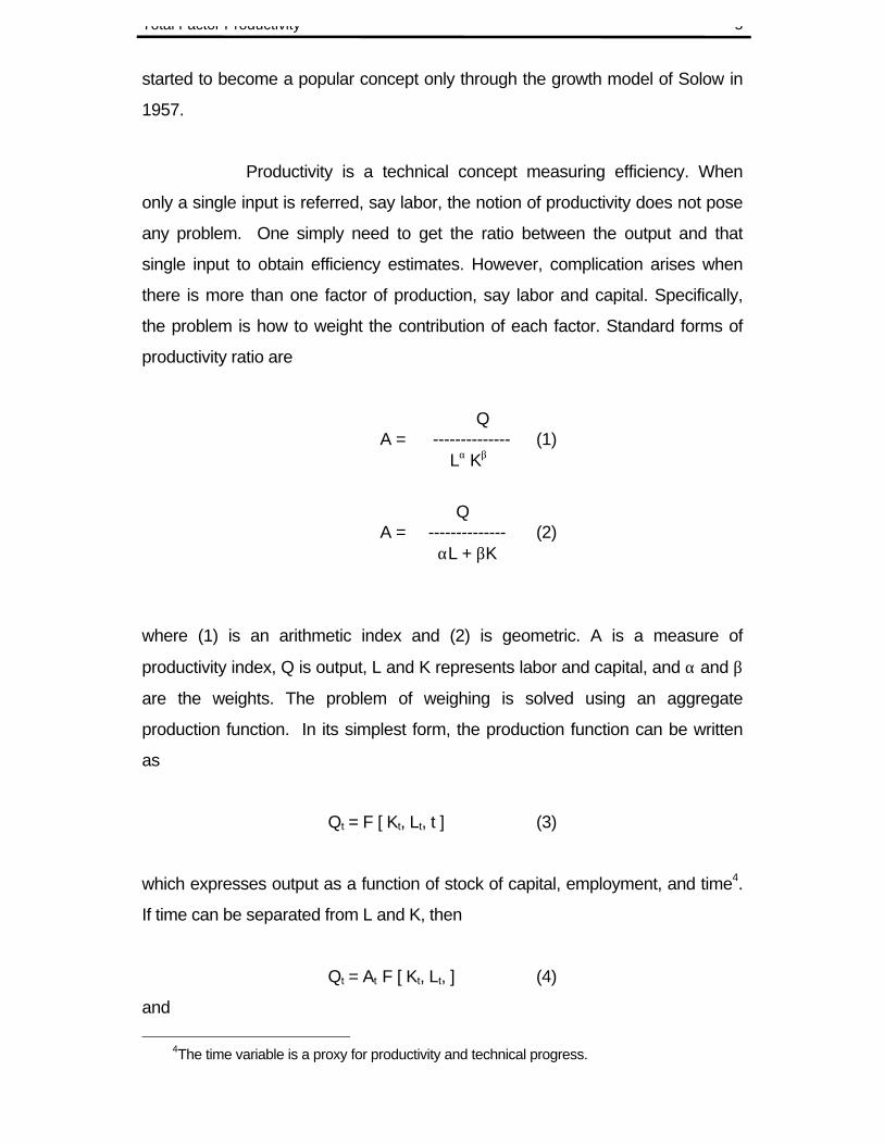
Productivity is a technical concept measuring efficiency. When
only a single input is referred, say labor, the notion of productivity does not pose
any problem. One simply need to get the ratio between the output and that
single input to obtain efficiency estimates. However, complication arises when
there is more than one factor of production, say labor and capital. Specifically,
the problem is how to weight the contribution of each factor. Standard forms of
productivity ratio are
QA = -------------- (1)
Lα Kβ
QA = -------------- (2) αL + βK
where (1) is an arithmetic index and (2) is geometric. A is a measure of
productivity index, Q is output, L and K represents labor and capital, and α and β
are the weights. The problem of weighing is solved using an aggregate
production function. In its simplest form, the production function can be written
as
Qt = F [ Kt, Lt, t ] (3)
which expresses output as a function of stock of capital, employment, and time4.
If time can be separated from L and K, then
Qt = At F [ Kt, Lt, ] (4)
and
4The time variable is a proxy for productivity and technical progress.
Total Factor Productivity 6
Qt
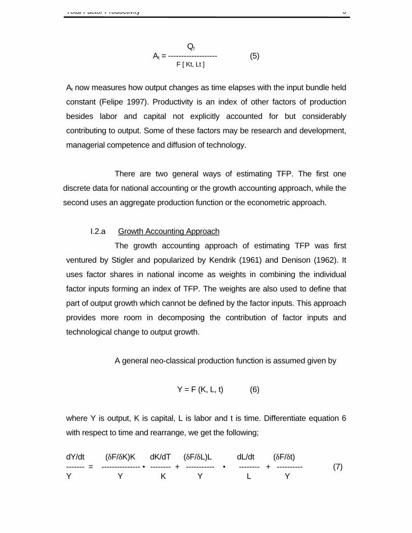
At = ------------------- (5) F [ Kt, Lt ]
At now measures how output changes as time elapses with the input bundle held
constant (Felipe 1997). Productivity is an index of other factors of production
besides labor and capital not explicitly accounted for but considerably
contributing to output. Some of these factors may be research and development,
managerial competence and diffusion of technology.
There are two general ways of estimating TFP. The first one
discrete data for national accounting or the growth accounting approach, while the
second uses an aggregate production function or the econometric approach.
I.2.a Growth Accounting Approach
The growth accounting approach of estimating TFP was first
ventured by Stigler and popularized by Kendrik (1961) and Denison (1962). It
uses factor shares in national income as weights in combining the individual
factor inputs forming an index of TFP. The weights are also used to define that
part of output growth which cannot be defined by the factor inputs. This approach
provides more room in decomposing the contribution of factor inputs and
technological change to output growth.
A general neo-classical production function is assumed given by
Y = F (K, L, t) (6)
where Y is output, K is capital, L is labor and t is time. Differentiate equation 6
with respect to time and rearrange, we get the following;
dY/dt (δF/δK)K dK/dT (δF/δL)L dL/dt (δF/δt)------- = --------------- • -------- + ----------- • -------- + ---------- (7)Y Y K Y L Y
Total Factor Productivity 7
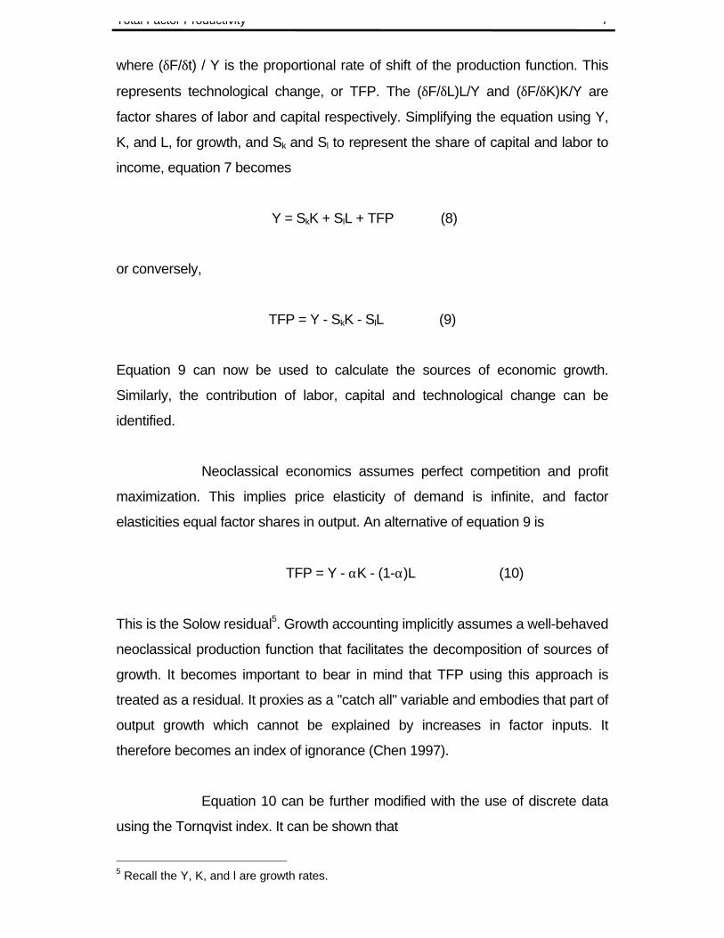
where (δF/δt) / Y is the proportional rate of shift of the production function. This
represents technological change, or TFP. The (δF/δL)L/Y and (δF/δK)K/Y are
factor shares of labor and capital respectively. Simplifying the equation using Y,
K, and L, for growth, and Sk and Sl to represent the share of capital and labor to
income, equation 7 becomes
Y = SkK + SlL + TFP (8)
or conversely,
TFP = Y - SkK - SlL (9)
Equation 9 can now be used to calculate the sources of economic growth.
Similarly, the contribution of labor, capital and technological change can be
identified.
Neoclassical economics assumes perfect competition and profit
maximization. This implies price elasticity of demand is infinite, and factor
elasticities equal factor shares in output. An alternative of equation 9 is
TFP = Y - αK - (1-α)L (10)
This is the Solow residual5. Growth accounting implicitly assumes a well-behaved
neoclassical production function that facilitates the decomposition of sources of
growth. It becomes important to bear in mind that TFP using this approach is
treated as a residual. It proxies as a "catch all" variable and embodies that part of
output growth which cannot be explained by increases in factor inputs. It
therefore becomes an index of ignorance (Chen 1997).
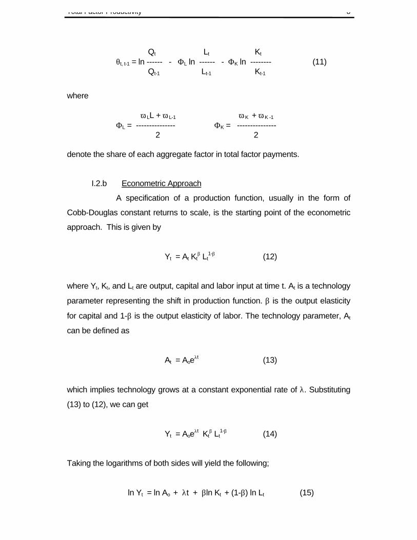
Equation 10 can be further modified with the use of discrete data
using the Tornqvist index. It can be shown that
5 Recall the Y, K, and l are growth rates.
Total Factor Productivity 8
Qt Lt Kt
θt, t-1 = ln ------ - ΦL ln ------ - ΦK ln -------- (11) Qt-1 Lt-1 Kt-1
where
ω LL + ω L-1 ω K + ω K -1
ΦL = --------------- ΦK = --------------- 2 2
denote the share of each aggregate factor in total factor payments.
I.2.b Econometric Approach
A specification of a production function, usually in the form of
Cobb-Douglas constant returns to scale, is the starting point of the econometric
approach. This is given by
Yt = At Ktβ Lt
1-β (12)
where Yt, Kt, and Lt are output, capital and labor input at time t. At is a technology
parameter representing the shift in production function. β is the output elasticity
for capital and 1-β is the output elasticity of labor. The technology parameter, At
can be defined as
At = Aoeλt (13)
which implies technology grows at a constant exponential rate of λ. Substituting
(13) to (12), we can get
Yt = Aoeλt Kt
β Lt1-β (14)
Taking the logarithms of both sides will yield the following;
ln Yt = ln Ao + λt + βln Kt + (1-β) ln Lt (15)
Total Factor Productivity 9
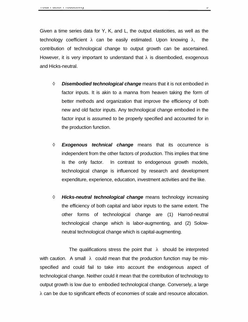
Given a time series data for Y, K, and L, the output elasticities, as well as the
technology coefficient λ can be easily estimated. Upon knowing λ, the
contribution of technological change to output growth can be ascertained.
However, it is very important to understand that λ is disembodied, exogenous
and Hicks-neutral.
◊ Disembodied technological change means that it is not embodied in
factor inputs. It is akin to a manna from heaven taking the form of
better methods and organization that improve the efficiency of both
new and old factor inputs. Any technological change embodied in the
factor input is assumed to be properly specified and accounted for in
the production function.
◊ Exogenous technical change means that its occurrence is
independent from the other factors of production. This implies that time
is the only factor. In contrast to endogenous growth models,
technological change is influenced by research and development
expenditure, experience, education, investment activities and the like.
◊ Hicks-neutral technological change means technology increasing
the efficiency of both capital and labor inputs to the same extent. The
other forms of technological change are (1) Harrod-neutral
technological change which is labor-augmenting, and (2) Solow-
neutral technological change which is capital-augmenting.
The qualifications stress the point that λ should be interpreted
with caution. A small λ could mean that the production function may be mis-
specified and could fail to take into account the endogenous aspect of
technological change. Neither could it mean that the contribution of technology to
output growth is low due to embodied technological change. Conversely, a large
λ can be due to significant effects of economies of scale and resource allocation.
Total Factor Productivity 10
Bias can also persist when important variables like research and development
(R&D), and education are not explicitly defined in the production function.
A variation of the econometric approach is the stochastic
approach. Equation 15 is based on a production function that expresses the
maximum obtainable output from a given set of inputs. However, empirical
models using ordinary least squares estimation can only obtain the average
production functions. For the best practice or production frontier methodology, an
unobservable production is assumed and this represents the set of maximum
attainable output level for a given combination of inputs. This approach
decomposes changes in TFP into technical progress and technical efficiency
change. Technical progress is associated with the best practice production
frontier, while the technical efficiency change is related to learning by doing,
improved managerial practice and changes in efficiency when a known
technology is applied (Kalirajan 1994).
I.3 Some Methodologies
Data availability and reliability differ among countries. Hence, a
comparable TFP estimate for international countries is close to impossible.
Added to this, the measurement of TFP depends on three things;
I. specification of the relationship between input and output
II. proper measurement of the factor inputs
III. weights assigned to the different categories of an input in the
aggregation of sub-inputs
In the earlier literature, Cobb-Douglas, CES, and VES6 were the
widely used production functions in estimating TFP. Recent development in the
growth literature shows that the most popular form of production function is the
transcendental logarithmic production function, or simply the translog production
function. This is specified as follows;
6 CES is Constant Elasticity of Substitution and VES is Variable Elasticity of Substitution.
Total Factor Productivity 11
Y = exp [ αo +α L ln L + αK ln K + αT T
+ ½ βKK ( ln K)2 + βKL ln K ln L + βKK T • ln K
+ ½ βLL (ln L)2 + βLT ln L • T + ΩβTT T2 ] (16)
The production function states that output is an exponential
function of the logarithms of the inputs. The translog function is a more
generalized form of the Cobb-Douglas and CES, and is much more favorable to
use because (1) it is not constrained by the restrictions similar in CES; and (2) it
provides a theoretical justification for the use of average factor shares in the
calculation of productivity growth.
The translog form can further be extended to treat aggregate
output as a function of its components. The translog form has provided
justification for the use of the growth accounting approach. However, problems in
the estimation still exist and these can be attributed to the measurement of factor
input.
I.4 Factor Input Measurement
The studies of Young (1992) and Krugman (1994) were the first of
a series of studies that dispelled the Asian miracle. Specifically, they stressed
that much of the output growth is driven by capital accumulation and not by
technological change and productivity. The relatively small TFP growth estimated
by these authors could be reflective of the biases in the measurement of factor
inputs.
Complications in the labor data may arise due to aggregation
problems. Each worker values labor quality differently. To account for the
changes in average work quality, adjustments are made using the age, sex, and
education of the labor force. These adjustments can partially explain the decline
in the growth of output per hour of labor input.7 Another issue that should be
7 See Clark (1979) for a detailed discussion of labor data adjustments.
Total Factor Productivity 12
addressed in the labor data is the effect of capital intensity on the growth of labor
productivity. Using “hours worked” as the standard measure of labor input, it
would be possible that adjustments for full-time equivalence can account for the
decline in the workweek of capital. Lastly, a distinction should be made between
number of hours and number of employees for labor data. Differences between
the two can arise into two situations; first, increases in part-time workers, and
second, decline of capital intensity of production.
Between capital and labor, the measurement for capital is more
problematic. There are basically three possible issues in the measurement of
capital.
A. Composition of Capital Input. There are numerous items that can be
classified as capital goods like land, inventories, consumer goods and
durable goods. A consistent decision should be made as to what items
should be included in the composition of capital input. This is very
important since the content of capital input will affect the type of price
deflators that is needed in making quality adjustments. Value shares have
to be estimated as weights, hence factor prices need to be known.
B. Adjustment for capacity utilization. Capital input is subject to the
business cycle. During recession, it is clear that there is excess capacity
in the use of capital. To adjust for capacity utilization, two indices could be
used--unemployment rate as a measure of under-utilization of capital, and
power utilization rate.
C. Choice between Net or Gross Capital. It is argued that the use of net
capital (net of depreciation) has the tendency to overstate depreciation
because obsolescence is the dominant feature of depreciation, rather
than physical deterioration. Capital becomes obsolete in the economic
context because it has outlived its physical usefulness. However, it is still
capable of contributing to production (Chen 1997). Ideally, capital should
Total Factor Productivity 13
be adjusted for depreciation but not obsolescence. In reality, this is
impossible to practice. Thus, any over-depreciation will overstate the
residual or TFP estimate.
The measurement of TFP is marred by conceptual and
measurement errors. Its interpretation largely depends on which methodology
was used, and how factor inputs were measured.
I.5 TFP Estimates: Some Empirical Findings
I.5.a Regional Estimates
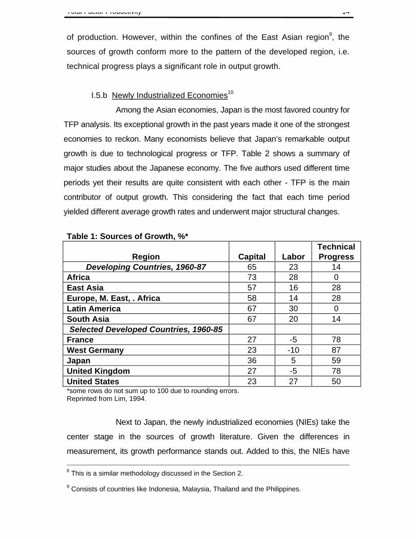
Numerous studies mushroomed analyzing the sources of growth
for both the developed and developing countries. In most cases, the
contribution of TFP to output growth for developed countries is significantly
high. Table 1 presents a regional summary of sources of growth published by
the World Bank (WB) in 1991. The WB Team used a Cobb-Douglas
production function and used differential calculus to arrive at the following8;
rQ = rT + αrK + βrL (17)
where rQ is the growth rate of output, rT is the growth rate of technical
progress, rK is the growth rate of capital and rL is the growth rate of labor.
From equation 17, they were able to decompose the sources of growth into
contribution of capital, labor and technological progress. The results are
consistent with those obtained in the earlier studies. In the developing
countries, the most important source of output growth is increases in capital
stock. For the entire region, accumulation of capital contributes 65 percent to
output growth, followed by labor contribution at 23 percent and lagging
behind is the contribution of technical progress at 14 percent. These findings
sharply contrast with that of the developed countries. According to the
estimates, technical progress largely accounts for the growth of output - a
case where efficiency in inputs is more relevant than accumulation of factors
Total Factor Productivity 14
of production. However, within the confines of the East Asian region9, the
sources of growth conform more to the pattern of the developed region, i.e.
technical progress plays a significant role in output growth.
I.5.b Newly Industrialized Economies10
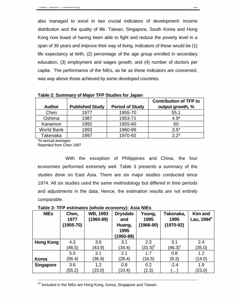
Among the Asian economies, Japan is the most favored country for
TFP analysis. Its exceptional growth in the past years made it one of the strongest
economies to reckon. Many economists believe that Japan’s remarkable output
growth is due to technological progress or TFP. Table 2 shows a summary of
major studies about the Japanese economy. The five authors used different time
periods yet their results are quite consistent with each other - TFP is the main
contributor of output growth. This considering the fact that each time period
yielded different average growth rates and underwent major structural changes.
Table 1: Sources of Growth, %*
Region Capital LaborTechnicalProgress
Developing Countries, 1960-87 65 23 14Africa 73 28 0East Asia 57 16 28Europe, M. East, . Africa 58 14 28Latin America 67 30 0South Asia 67 20 14Selected Developed Countries, 1960-85
France 27 -5 78West Germany 23 -10 87Japan 36 5 59United Kingdom 27 -5 78United States 23 27 50*some rows do not sum up to 100 due to rounding errors.Reprinted from Lim, 1994.
Next to Japan, the newly industrialized economies (NIEs) take the
center stage in the sources of growth literature. Given the differences in
measurement, its growth performance stands out. Added to this, the NIEs have
8 This is a similar methodology discussed in the Section 2.
9 Consists of countries like Indonesia, Malaysia, Thailand and the Philippines.
Total Factor Productivity 15
also managed to excel in two crucial indicators of development: income
distribution and the quality of life. Taiwan, Singapore, South Korea and Hong
Kong now boast of having been able to fight and reduce the poverty level in a
span of 30 years and improve their way of living. Indicators of these would be (1)
life expectancy at birth, (2) percentage of the age group enrolled in secondary
education, (3) employment and wages growth, and (4) number of doctors per
capita. The performance of the NIEs, as far as these indicators are concerned,
was way above those achieved by some developed countries.
Table 2: Summary of Major TFP Studies for Japan
Author Published Study Period of StudyContribution of TFP to
output growth, %Chen 1977 1955-70 55.1
Oshima 1987 1953-71 4.9*Kanamori 1992 1955-60 60
World Bank 1993 1960-89 3.5*Takenaka 1997 1970-92 2.2*
*In annual averagesReprinted from Chen 1997
With the exception of Philippines and China, the four
economies performed extremely well. Table 3 presents a summary of the
studies done on East Asia. There are six major studies conducted since
1974. All six studies used the same methodology but differed in time periods
and adjustments in the data. Hence, the estimation results are not entirely
comparable.
Table 3: TFP estimates (whole economy): Asia NIEsNIEs Chen,
1977(1955-70)
WB, 1993(1960-89)
Drysdaleand
Huang,1995
(1950-88)
Young,1995
(1966-90)
Takenaka,1995
(1970-92)
Kim andLau, 1994a
Hong Kong 4.3(46.5)
3.6(43.9)
3.1(34.4)
2.3(31.5)b
3.1(46.3)c
2.4(35.0)
Korea5.0
(56.4)3.1
(36.9)2.1
(28.4)1.7
(16.5)0.8
(9.3)1.2
(14.0)Singapore 3.6
(55.2)1.2
(15.0)0.8
(10.4)0.2
(2.3)-2.4(…)
1.9(23.0)
10 Included in the NIEs are Hong Kong, Korea, Singapore and Taiwan.
Total Factor Productivity 16
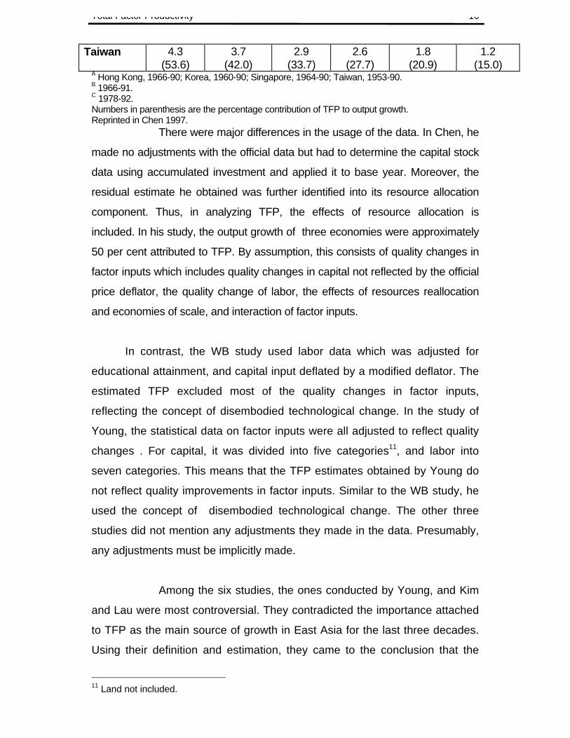
Taiwan 4.3(53.6)
3.7(42.0)
2.9(33.7)
2.6(27.7)
1.8(20.9)
1.2(15.0)
A Hong Kong, 1966-90; Korea, 1960-90; Singapore, 1964-90; Taiwan, 1953-90.B 1966-91.C 1978-92.Numbers in parenthesis are the percentage contribution of TFP to output growth.Reprinted in Chen 1997.
There were major differences in the usage of the data. In Chen, he
made no adjustments with the official data but had to determine the capital stock
data using accumulated investment and applied it to base year. Moreover, the
residual estimate he obtained was further identified into its resource allocation
component. Thus, in analyzing TFP, the effects of resource allocation is
included. In his study, the output growth of three economies were approximately
50 per cent attributed to TFP. By assumption, this consists of quality changes in
factor inputs which includes quality changes in capital not reflected by the official
price deflator, the quality change of labor, the effects of resources reallocation
and economies of scale, and interaction of factor inputs.
In contrast, the WB study used labor data which was adjusted for
educational attainment, and capital input deflated by a modified deflator. The
estimated TFP excluded most of the quality changes in factor inputs,
reflecting the concept of disembodied technological change. In the study of
Young, the statistical data on factor inputs were all adjusted to reflect quality
changes . For capital, it was divided into five categories11, and labor into
seven categories. This means that the TFP estimates obtained by Young do
not reflect quality improvements in factor inputs. Similar to the WB study, he
used the concept of disembodied technological change. The other three
studies did not mention any adjustments they made in the data. Presumably,
any adjustments must be implicitly made.
Among the six studies, the ones conducted by Young, and Kim
and Lau were most controversial. They contradicted the importance attached
to TFP as the main source of growth in East Asia for the last three decades.
Using their definition and estimation, they came to the conclusion that the
11 Land not included.
Total Factor Productivity 17
main driving force of the Asian miracle, it ever there was one, was capital
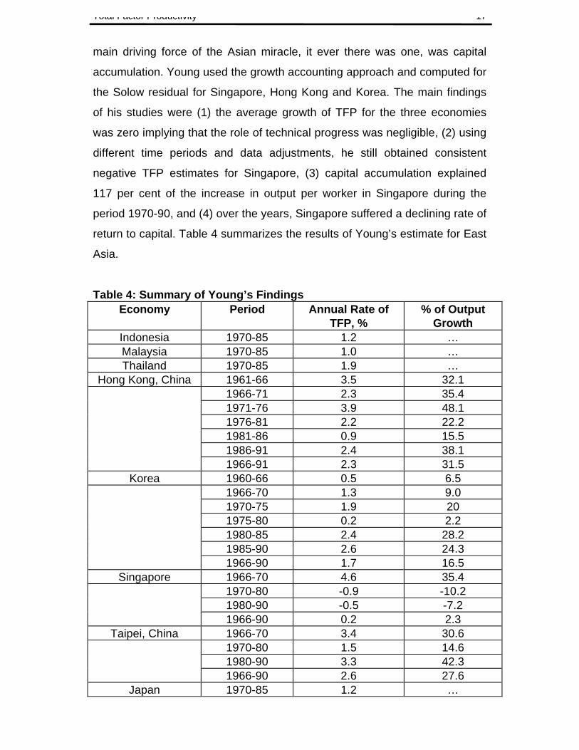
accumulation. Young used the growth accounting approach and computed for
the Solow residual for Singapore, Hong Kong and Korea. The main findings
of his studies were (1) the average growth of TFP for the three economies
was zero implying that the role of technical progress was negligible, (2) using
different time periods and data adjustments, he still obtained consistent
negative TFP estimates for Singapore, (3) capital accumulation explained
117 per cent of the increase in output per worker in Singapore during the
period 1970-90, and (4) over the years, Singapore suffered a declining rate of
return to capital. Table 4 summarizes the results of Young’s estimate for East
Asia.
Table 4: Summary of Young’s FindingsEconomy Period Annual Rate of
TFP, %% of Output
GrowthIndonesia 1970-85 1.2 …Malaysia 1970-85 1.0 …Thailand 1970-85 1.9 …
Hong Kong, China 1961-66 3.5 32.11966-71 2.3 35.41971-76 3.9 48.11976-81 2.2 22.21981-86 0.9 15.51986-91 2.4 38.11966-91 2.3 31.5
Korea 1960-66 0.5 6.51966-70 1.3 9.01970-75 1.9 201975-80 0.2 2.21980-85 2.4 28.21985-90 2.6 24.31966-90 1.7 16.5
Singapore 1966-70 4.6 35.41970-80 -0.9 -10.21980-90 -0.5 -7.21966-90 0.2 2.3
Taipei, China 1966-70 3.4 30.61970-80 1.5 14.61980-90 3.3 42.31966-90 2.6 27.6
Japan 1970-85 1.2 …
Total Factor Productivity 18
… not available.Reprinted from Felipe 1997.
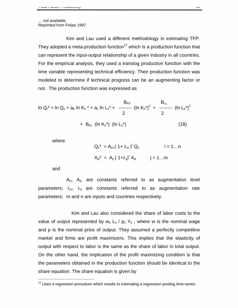
Kim and Lau used a different methodology in estimating TFP.
They adopted a meta-production function12 which is a production function that
can represent the input-output relationship of a given industry in all countries.
For the empirical analysis, they used a translog production function with the
time variable representing technical efficiency. Their production function was
modeled to determine if technical progress can be an augmenting factor or
not. The production function was expressed as
BKK BLL
ln Qt* = ln Qo + aK ln Kit * + aL ln Lit* + -------- (ln Kit*)2 + -------- (ln Lit*)
2
2 2
+ BKL (ln Kit*) (ln Lit*) (18)
whereQit* = Aiio ( 1+ λio )
t Qit i = 1…n
Xijt* = Aij ( 1+λij)t Xijt j = 1…m
and
Aio, Aij, are constants referred to as augmentation level
parameters; λio, λij are constants referred to as augmentation rate
parameters; m and n are inputs and countries respectively.
Kim and Lau also considered the share of labor costs to the
value of output represented by wit Lit / pit Yit , where w is the nominal wage
and p is the nominal price of output. They assumed a perfectly competitive
market and firms are profit maximizers. This implies that the elasticity of
output with respect to labor is the same as the share of labor in total output.
On the other hand, the implication of the profit maximizing condition is that
the parameters obtained in the production function should be identical to the
share equation. The share equation is given by
12 Uses a regression procedure which results to estimating a regression pooling time-series
Total Factor Productivity 19
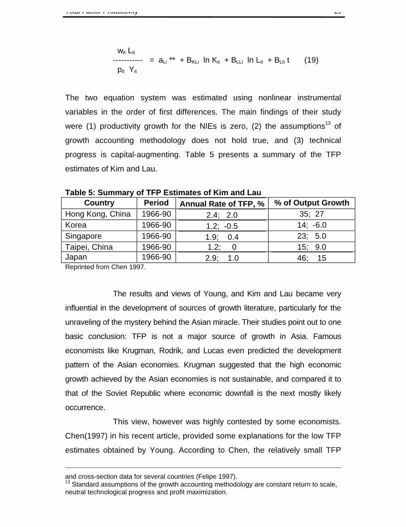
wit Lit
----------- = aLi ** + BKLi ln Kit + BLLi ln Lit + BLti t (19) pit Yit
The two equation system was estimated using nonlinear instrumental
variables in the order of first differences. The main findings of their study
were (1) productivity growth for the NIEs is zero, (2) the assumptions13 of
growth accounting methodology does not hold true, and (3) technical
progress is capital-augmenting. Table 5 presents a summary of the TFP
estimates of Kim and Lau.
Table 5: Summary of TFP Estimates of Kim and LauCountry Period Annual Rate of TFP, % % of Output Growth
Hong Kong, China 1966-90 2.4; 2.0 35; 27Korea 1966-90 1.2; -0.5 14; -6.0Singapore 1966-90 1.9; 0.4 23; 5.0Taipei, China 1966-90 1.2; 0 15; 9.0Japan 1966-90 2.9; 1.0 46; 15Reprinted from Chen 1997.
The results and views of Young, and Kim and Lau became very
influential in the development of sources of growth literature, particularly for the
unraveling of the mystery behind the Asian miracle. Their studies point out to one
basic conclusion: TFP is not a major source of growth in Asia. Famous
economists like Krugman, Rodrik, and Lucas even predicted the development
pattern of the Asian economies. Krugman suggested that the high economic
growth achieved by the Asian economies is not sustainable, and compared it to
that of the Soviet Republic where economic downfall is the next mostly likely
occurrence.
This view, however was highly contested by some economists.
Chen(1997) in his recent article, provided some explanations for the low TFP
estimates obtained by Young. According to Chen, the relatively small TFP
and cross-section data for several countries (Felipe 1997).13 Standard assumptions of the growth accounting methodology are constant return to scale,neutral technological progress and profit maximization.
Total Factor Productivity 20
estimate Young obtained in his computations does not necessarily imply that
technological change is an insignificant source of growth. A more appropriate
explanation, as Chen suggested, would be disembodied technological
change did not play an important role in the economic growth but embodied
technological change added with quality improvements could have been the
more important player of growth for developing countries. Further, he claims
that what can be inferred from these studies is that embodied technological
change is more relevant for developing countries while disembodied
technological change is the major player for developed countries. He
contradicted the views of Krugman by claiming that technological change, in
the embodied form, has been significant in East Asia (Chen 1997).
I.5.c Southeast Asia14
There are only very few studies made for Southeast Asia, and
some of the earlier studies were TFP estimates for the Philippines. In the
recent studies, the four countries were categorized into forces that push for
output growth. Indonesia and Thailand are classified as productivity-driven
economies because TFP contributes for more than 25 per cent of economic
growth. For Indonesia, studies showed that its industrial sector has grown
significantly over time. For Philippines and Malaysia, these economies are
classified as investment-driven growth where there is little or no productivity
growth at all. Table 6 shows a summary of the studies conducted for
Southeast Asia.
I.5.d Philippines
During the 80s when Asian economies were experiencing high
levels of growth, the Philippines was struggling from economic bondage and was
forced to implement structural adjustments dictated by the World Bank and the
International Monetary Fund. The adjustment policies were aimed at correcting
the balance of payment deficit and reducing the fiscal deficit which unfortunately
led to a deterioration of the living standards of the Filipinos and large drop in
14 Southeast Asian economies include Indonesia, Malaysia, Philippines, and Thailand.
Total Factor Productivity 21
economic growth (Kajiwara 1994). Aside from macroeconomic imbalance, the low
productivity level of the Philippine economy was considered one of the significant
factors which led to the failure of attaining industrialization. Based on the
literature, only a handful of studies were conducted pertaining to the productivity
of the Philippine economy. In spite of the differences in the methodology, time
frame and data set used in all these studies, each arrived at the same
conclusion: a declining productivity estimate. Recent papers on productivity
were conducted by Cororaton et al (1995, 1997), Austria and Martin (1992) and
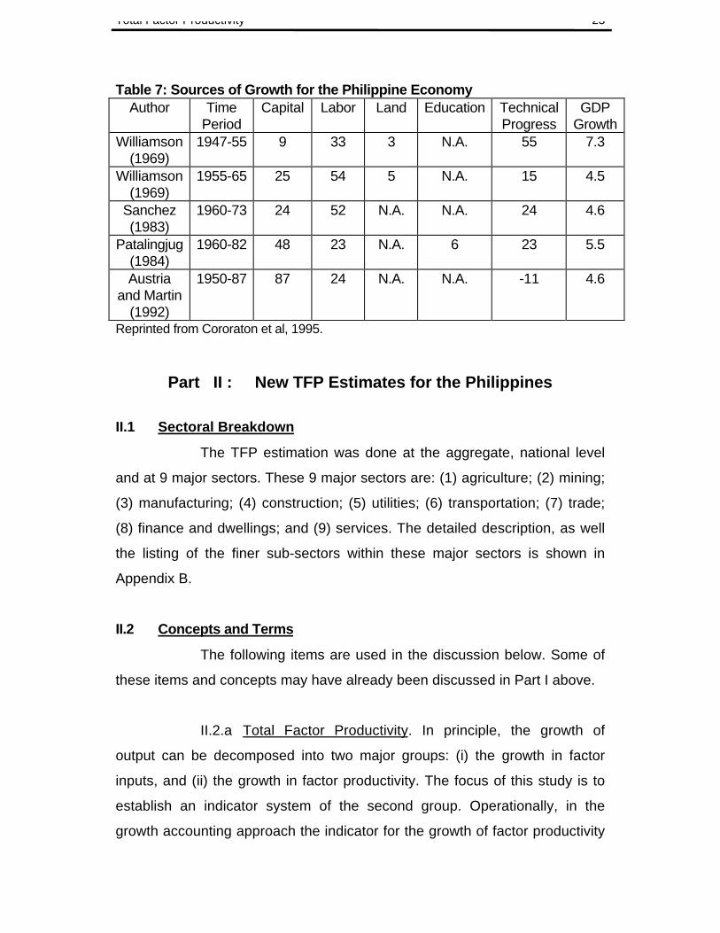
Patalingjug (1984). Cororaton attributed the declining TFP from poor acquisition
of technology while Austria and martin delved into the different trade and
investment policies. Table 7 presents a summary of the various studies
conducted for the Philippine economy.
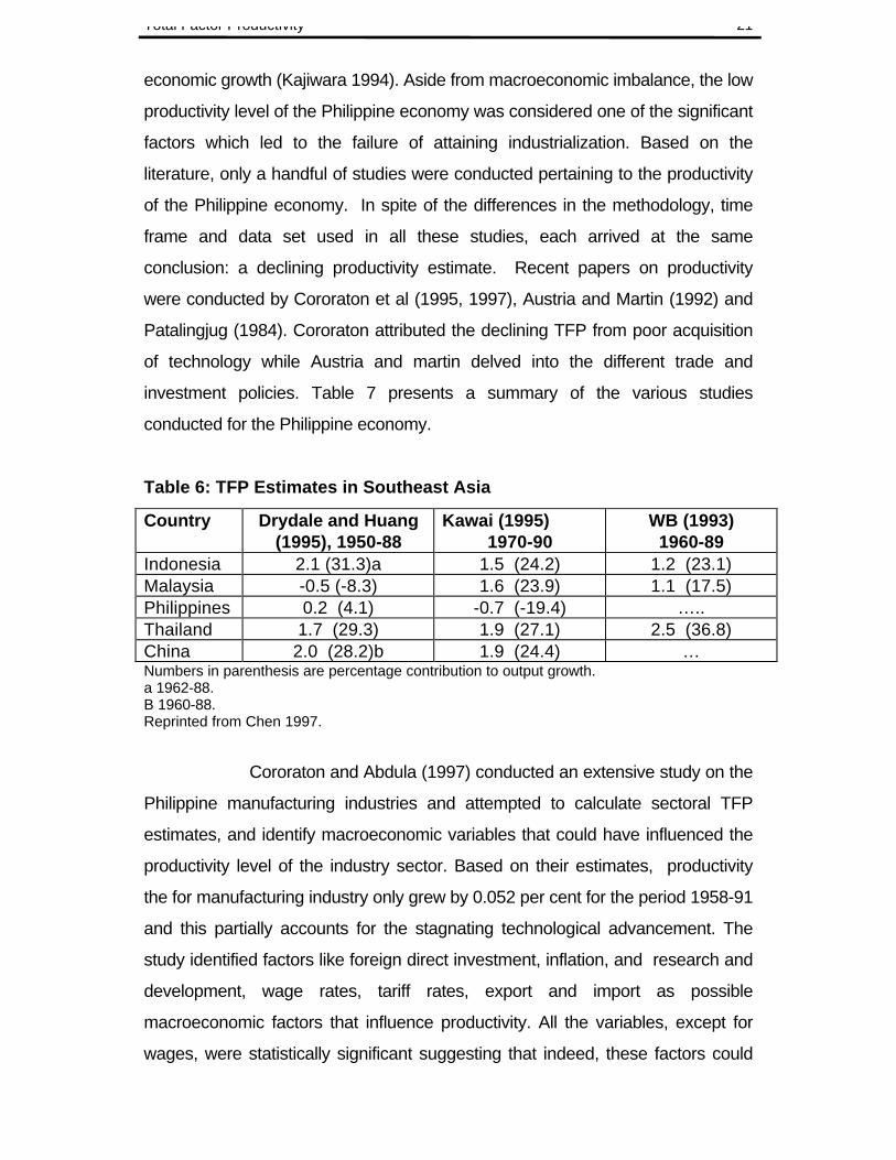
Table 6: TFP Estimates in Southeast Asia
Country Drydale and Huang(1995), 1950-88
Kawai (1995)1970-90
WB (1993)1960-89
Indonesia 2.1 (31.3)a 1.5 (24.2) 1.2 (23.1)Malaysia -0.5 (-8.3) 1.6 (23.9) 1.1 (17.5)Philippines 0.2 (4.1) -0.7 (-19.4) …..Thailand 1.7 (29.3) 1.9 (27.1) 2.5 (36.8)China 2.0 (28.2)b 1.9 (24.4) …Numbers in parenthesis are percentage contribution to output growth.a 1962-88.B 1960-88.Reprinted from Chen 1997.
Cororaton and Abdula (1997) conducted an extensive study on the
Philippine manufacturing industries and attempted to calculate sectoral TFP
estimates, and identify macroeconomic variables that could have influenced the
productivity level of the industry sector. Based on their estimates, productivity
the for manufacturing industry only grew by 0.052 per cent for the period 1958-91
and this partially accounts for the stagnating technological advancement. The
study identified factors like foreign direct investment, inflation, and research and
development, wage rates, tariff rates, export and import as possible
macroeconomic factors that influence productivity. All the variables, except for
wages, were statistically significant suggesting that indeed, these factors could

Total Factor Productivity 22
influence productivity growth. These results entail policy implication. A sound
macroeconomic environment would stimulate investment and improve
productivity. Stabilization policies like low inflation and reduced budget deficits
are attractive to investors.
Total Factor Productivity 23
Table 7: Sources of Growth for the Philippine EconomyAuthor Time
PeriodCapital Labor Land Education Technical
ProgressGDP
GrowthWilliamson
(1969)1947-55 9 33 3 N.A. 55 7.3
Williamson(1969)
1955-65 25 54 5 N.A. 15 4.5
Sanchez(1983)
1960-73 24 52 N.A. N.A. 24 4.6
Patalingjug(1984)
1960-82 48 23 N.A. 6 23 5.5
Austriaand Martin
(1992)
1950-87 87 24 N.A. N.A. -11 4.6
Reprinted from Cororaton et al, 1995.
Part II : New TFP Estimates for the Philippines
II.1 Sectoral Breakdown
The TFP estimation was done at the aggregate, national level
and at 9 major sectors. These 9 major sectors are: (1) agriculture; (2) mining;
(3) manufacturing; (4) construction; (5) utilities; (6) transportation; (7) trade;
(8) finance and dwellings; and (9) services. The detailed description, as well
the listing of the finer sub-sectors within these major sectors is shown in
Appendix B.
II.2 Concepts and Terms
The following items are used in the discussion below. Some of
these items and concepts may have already been discussed in Part I above.
II.2.a Total Factor Productivity. In principle, the growth of
output can be decomposed into two major groups: (i) the growth in factor
inputs, and (ii) the growth in factor productivity. The focus of this study is to
establish an indicator system of the second group. Operationally, in the
growth accounting approach the indicator for the growth of factor productivity
Total Factor Productivity 24
is computed residually15. That is, if the indicator of output growth is the growth
of real GVA, then factor productivity (or total factor productivity growth) is
calculated as the difference between the real growth in GVA and the
weighted sum of the growth of the primary factor inputs which are labor and
capital16. As such, TFP is calculated as a growth rate, since it is the
difference between two growth rates. Normally, it is not derived in monetary
units or in levels.
Why focus on the growth in factor productivity? The growth in
the primary factors (commonly called as factor accumulation) is subject to
diminishing returns. Therefore, the growth in output due to factor
accumulation will eventually taper off, making the growth process
unsustainable in the long run. However, the growth in factor productivity has
increasing returns characteristics. That is, there is no limit to the growth in
output that is due to factor productivity. 17
Theoretically, factor productivity growth can be decomposed
into major sub-groups: technical efficiency and technical progress which are
discussed below.
II.2.b Technical Efficiency. Technical efficiency is defined as
the degree of effectiveness of the operation of the organisation in being able
15 TFP indicator may also be derived econometrically. Under such approach the coefficient ofone of the variables in the regression of the production function is an estimate of TFP.However, the TFP result will be an average over the regression period. Year-to-year variationof TFP may not be analyzed in this case.
16Some studies consider different skill levels of labor and different qualities of capital. Othersalso include land. The present study, however, does not consider different labor skills andcapital qualities and land. In effect, the effect of improvements in the quality of factor inputsare all lumped up in the TFP estimate. An interesting area for research is to include thedifferent input characteristics. In principle, this should reduce the size of TFP.
17 As discussed in Part I, there are generally two schools of thought about the things thatpropel factor productivity growth: the old neoclassical school which states that the productionfrontier of developing countries approaches or converges naturally to that of the developedcountries in the long run. In the new school, which is called the endogenous growth theory,convergence may not happen naturally and automatically. In fact, it requires active policyintervention in areas like education, population, research and development, trade reforms,market reforms, foreign direct investment, transfer of technology, etc..
Total Factor Productivity 25
to produce an output level that is at its potential, given its present capacity.
Simply put, technical efficiency measures how near the organisation is
operating from its production frontier. There are a number of things that can
affect the technical efficiency of an organisation. One would be the effectivity
of management. Another would be the efficiency of the structure of the
organisation. However, the important point to consider here is that the
improvement in output due to the improvement in technical efficiency is
realised not through an additional investment, but through an improvement in
the existing set-up of the organisation, e.g., effective management, efficient
production operation, etc.
II.2.c. Technical Progress. Technical progress is defined as the
improvement in the output potential itself of the organisation. Theoretically, it
is defined as the upward shift in the production frontier itself, as opposed to
technical efficiency defined above as the movement towards the present
production frontier. The factors that may affect such shifts include: technology
transfer, investment in human capital, investment in research development,
etc.
Thus, the TFP indicator, as a productivity indicator, captures
changes in technical efficiency and technical progress.
II.3 Data Base
The TFP estimation in the study was done both at the national
and the sectoral level. The strategy followed was to start at the national level,
utilising information from the national income accounts (NIA). From the
national level, data for the sectoral level analysis were constructed using
appropriate distribution shares. This strategy was adopted because NIA is
updated regularly. Thus, with regular updates of the NIA, regular TFP
updates can also be done. Furthermore, this strategy has another advantage
of reducing the possibility of accumulated error at the national level TFP
Total Factor Productivity 26
estimates. If it were from the sectoral up to the national, then data errors that
may be committed at the sectors may add up so that the accumulated error at
the national level may be huge.
Because of data constraints the TFP estimation covers only the
period 1980 to 1996. It would have been better to extend the analysis further
back to the 1970s and 1960s to get a longer-term perspective of the TFP
movements. However, one of the major set of information used in the
estimation of TFP, which is the factor payment shares at the sectoral level, is
available only starting from 1980. A detailed, step-by-step procedure used to
construct the data base is shown in Appendix B.
Gross value added. The indicator of value of output used in the
estimation is gross value added (GVA). The reason for doing this is that
gross domestic product (GDP) in the NIA is the sum of sectoral GVA. Since
updates for both GDP and sectoral GVA come out regularly, it is possible to
do regular updates for the TFP indicators at both levels. Furthermore, factor
payments to labor and capital (wage compensation, and mixed income and
operating surplus, respectively) at sectoral level are also available regularly
on an annual basis. Thus, with GVA, the effects coming from the raw
materials are not accounted for in the TFP estimates.
Both GDP and sectoral GVA were expressed in real prices
using their respective implicit price indexes, which are also available from the
NIA. The price indexes are in 1985 prices.
Labor. Data on employment, both at the national and sectoral
level are published regularly. Thus, in the TFP estimation, the data series on
the number of employment generated by the Department of Labor and
Employment (DOLE) were utilised as labor factor input. In principle, labor
service, not the level of employment, is the one that is relevant in the
analysis. The common practise is to adjust the employment data with some
Total Factor Productivity 27
information on average working hours. However, a good time series for the
“weekly average hours work” is not available. Because of this problem, the
employment data were not adjusted. For the time being, this presents one
weakness in the estimation, which can be easily modified and adjusted after a
good and consistent “weekly average hours work” time data series has been
established.
Capital Stock. Usually, one of the major problems encountered
in TFP estimation is the unavailability of capital stock series both at the
national and sectoral level. In the Philippines, the problem is aggravated by
the unavailability of sectoral investment data series. Appendix B shows a
detailed procedure used to construct capital stock series at the national and
sectoral level. In essence, the procedure started with the gross domestic
capital formation GDCF (investment at the national level) which is available
from the NIA. This GDCF series was distributed into sectoral investment
using a set of derived sectoral investment shares computed using the
sectoral gross additions to fixed assets (GAFA) from the Annual Survey of
Establishment (ASE) of the National Statistics Office (NSO). The capital stock
series were derived using the perpetual inventory method18.
Capacity Utilisation Capital services are the ones needed in the
analysis, instead of the level of capital stock. To arrive at this set of
information, the derived capital stock series were adjusted by capacity
utilisation. In the study capacity utilisation index was derived using the peak-
to-peak method on both real GDP and real sectoral GVA. A detailed analysis
appears in Appendix B.
II.4 TFP Methodologies Used.
18The task of computing for the sectoral investment would have been a lot easier and theresult would have been more accurate if sectoral investment were available. However, thereis an ongoing effort in the National Statistical Coordination Board (NSCB) to construct a timeseries for sectoral investment. The derived investment series in this paper can be checked
Total Factor Productivity 28
There are a number of approaches to estimating TFP available
in the literature. As discussed above, the different approaches fall under (a)
the growth accounting approach, and (b) the production function and the
econometric estimation approach. In the present study few methodologies
under each approach were applied. For the first approach two methodologies
were used: the traditional growth accounting methodology (Method 1) and the
translog index method (also called the Tornquist Method, Method 2). For the
second approach, a Cobb-Douglas production function was estimated
econometrically (Method 3), as well as the stochastic frontier (Method 4).
Each of these methods are discussed below.
Growth Accounting Method (Method 1). The traditional growth
accounting approach was applied both on the annual changes in value added
and factor inputs, and on the three-year moving averages of these changes.
The latter was done to smooth out the annual variability of the changes of the
value added and factor input series. To reiterate, growth accounting
approach uses the following formula:
(TFP growth)i = (value added growth)i - ΘLi* (employment growth)i –
ΘKi * (capital services growth) i (20)
growth where value added growth was computed using data in Table A1 in
Appendix A; employment growth computed using Table A3, capital services
growth computed using the product of capital stock series (Table A7) and
capacity utilization (Table A6), and ΘLi and ΘKi are factor payment shares in
Table A2. One should note that the employment data was not adjusted for
average hours of work in order to derive the appropriate labor services. This
is because of the unavailability of a consistent series on average hours of
work. However, the derived capital stock series was adjusted for capacity
utilization to get capital services. The advantage of using this approach is
that is it straight forward to apply. The usual problems in regression analysis
against these numbers when they come out officially. If there are significant deviations, thenthe estimates of this paper will be revised accordingly.

Total Factor Productivity 29
are not encountered. However, the test of statistical significance of the
estimates cannot be conducted.
Translog Index Approach (Method 2). The translog index
approach is
Total Factor Productivity 30
TFPi = [ lnQi(t) – lnQi(t-1) ] – viL * [ lnLi(t) – lnLi(t-1) ] –
viK * [ lnKi(t) – lnKi(t-1) ] (21)
where viL = ½ * ( viL(t) – viL(t-1) )
viK = ½ * (viK(t) – viK(t-1))
where ln is natural logarithm operator, Qi value added of sector i, viL, viK
average factor shares, Li employment, and Ki is capital service. This method
is also straight forward to apply. It can generate annual estimates of TFP,
thus can easily be monitored. However, similar to Method 1, the results
cannot be tested for statistical significance.19
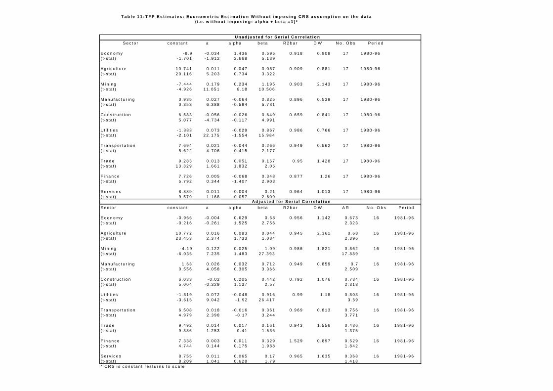
Econometric Method (Method 3). This method uses a
regression analysis on a Cobb-Douglas production function specification.
That is
ln Qi = CONST + at + α lnLi + β ln Ki + eI (22)
where Qi is value added of sector i, CONST is a constant term in the
regression, a is the coefficient of the time trend, t, (which is interpreted as
the average TFP for sector i over the regression period which is 1980-1996),
α coefficient of labor, Li (which is also the labor factor share under perfect
competition), β coefficient of capital, Ki (capital factor share), and ei an error
term with the usual properties.
This specification was applied on the constructed data using
two ways: (i) without imposing the assumption of constant returns to scale
(CRS) on the data; and (ii) with CRS. CRS implies α + β = 1.
The advantage of this method is that the result can be tested for
statistical significance. However, the result will only give an estimate of the
19The advantage of Method 2 over 1 is that, under certain conditions, the production
Total Factor Productivity 31
average TFP over the regression period. The annual variations of the TFP
cannot be analysed, thus difficult to monitor.
Frontier Approach (Method 4). This is also an econometric-
based method. However, the analytics behind this method is different from
that of Method 3. In Method 3, one of the major assumptions is that the sector
is operating at its potential. That is, it is operating along its production
frontier. Therefore, the issue of technical efficiency is not considered
explicitly. In Method 4 this is accounted for in the specification of the
estimating function.
In the study, Method 4 is applied not for the purpose of
computing for TFP estimates but for generating estimates of sectoral
technical efficiency, in the form of coefficients, of the 9 sectors. The
coefficient indicates how well the sector performs relative to the best practise
frontier. If the coefficient is 100 percent, it means that the sector operates
along the frontier. However, if the coefficient is below 100, for example 50
percent only, it means that it is producing an output level which is 50 percent
below its potential. The best practise frontier was computed using sectoral
data on value added and factor inputs.20
The best practice, production function can be represented as
QFt = f[Xt, t] (23)
technology of 2 is more flexible, being translog, than 1 which is Cobb-Douglas.20This method, as applied in the present context, has a major weakness. In principle, thismethod is appropriate to firm-level data or to an industry with more or less similartechnology. However, in the present study, this may not be so since it is applied to 9 broadsectors, which may or may not have similar or comparable technology. The presenttechnology in agriculture, for example, may be totally different from the level of technologyin the manufacturing sector. In other words, the production frontier of agriculture may not becomparable with the current frontier of the manufacturing sector. Ideally, the technology of aparticular sector, say manufacturing, is compared across countries. The best practise frontieris calculated using the manufacturing performance of other countries, particularly efficientdeveloped countries. The Philippine manufacturing is compared against this frontier, as inWorld bank, 1993. However, this cannot be done at this point. Because of this, the resultsunder this approach should be considered with great care.
Total Factor Productivity 32
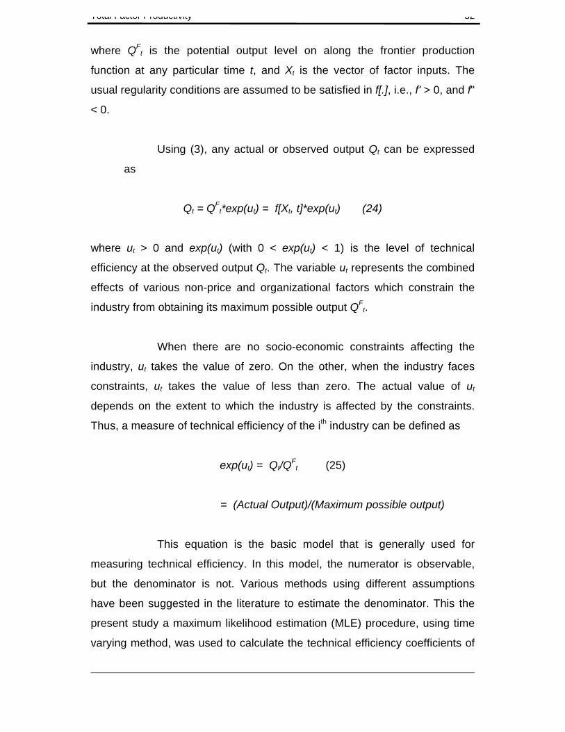
where QFt is the potential output level on along the frontier production
function at any particular time t, and Xt is the vector of factor inputs. The
usual regularity conditions are assumed to be satisfied in f[.], i.e., f' > 0, and f"
< 0.
Using (3), any actual or observed output Qt can be expressed
as
Qt = QFt*exp(ut) = f[Xt, t]*exp(ut) (24)
where ut > 0 and exp(ut) (with 0 < exp(ut) < 1) is the level of technical
efficiency at the observed output Qt. The variable ut represents the combined
effects of various non-price and organizational factors which constrain the
industry from obtaining its maximum possible output QFt.
When there are no socio-economic constraints affecting the
industry, ut takes the value of zero. On the other, when the industry faces
constraints, ut takes the value of less than zero. The actual value of ut
depends on the extent to which the industry is affected by the constraints.
Thus, a measure of technical efficiency of the ith industry can be defined as
exp(ut) = Qt/QF
t (25)
= (Actual Output)/(Maximum possible output)
This equation is the basic model that is generally used for
measuring technical efficiency. In this model, the numerator is observable,
but the denominator is not. Various methods using different assumptions
have been suggested in the literature to estimate the denominator. This the
present study a maximum likelihood estimation (MLE) procedure, using time
varying method, was used to calculate the technical efficiency coefficients of
Total Factor Productivity 33
the sectors. The MLE procedure was computed using the program
FRONTIER 4.1 (Coelli, 1994).
II.5 TFP Estimates
Table 8 shows the results of the growth accounting method
using 3-year moving averages of the value added and the factor input series,
while Table 9 shows the results of the same method without moving
averages. Table 10 shows the results of the translog method. Table 11 shows
the results of Method 3 without CRS assumption The relevant result is the
coefficient of t which is a. This particular coefficient is an estimate of the
average TFP over the regression period, which is 1980-1996. Note that there
are two sets of results for this particular method. The first set are the results
of the regression without correction for serial correction, while the second are
the results with correction. Note also that the results in the second set have
slightly improved DW statistics. Table 12 shows the results with CRS
assumption. Based on the regression, the results in Table 12 are better than
Table 1121. Table 13 shows the technical efficiency coefficients of the sectors
calculated using the stochastic frontier method.
The annual TFP estimates of both Methods 1 and 2 are shown
in Figures 1 to 10 for the entire economy and for the rest of the 9 major
sectors. Note that the trend of the TFP estimates using these two methods
move in the same general direction, although there are few annual variations.
TFP improved right after the crisis in the mid-1980s (Figure 1).
It was highest during the early years of the Aquino administration. However,
the improvement was not sustained. TFP dipped down in the early 1990s,
21Multi-collinearity and other time series problems created problems in regression withoutCRS assumption. These problems show up in the t-test of alpha and beta which are eitherstatistically insignificant or wrong sign. Thus, the results with CRS assumption are slightlybetter.
Total Factor Productivity 34
and has not improved since then. In fact, in the last six years, TFP of the
entire economy has been below zero.22
There are differences in the TFP performance at the sectoral
level. One surprising result concerns the TFP of agriculture (Figure 2). In the
last five years, TFP of agriculture is positive on the average. This is contrary
to the common perception of low productivity in this sector. It may be difficult
to pinpoint the factors behind this, but one reason may probably be that
technology is not embodied in capital input. It may be disembodied. In such a
case, technological change or improvement may probably due captured in the
residual, which is TFP. Thus a relatively higher TFP.
The TFP of the mining sector (Figure 3) declined to below zero
in 1995 and 1996. Before these years, TFP has been positive, although small
in magnitude.
TFP of the manufacturing sector registered an impressive
growth in the second half of the 1980s (Figure 4). It was averaging 5 percent
per year in 1987 to 1989. In the early 1990s, TFP slowed down to almost
zero, but recovered after that until it reached another peak in 1993 and 1994.
In the last two years it slowed down again. It even registered negative TFP in
1996.
The construction sector has not been performing well in terms if
TFP growth (Figure 5). In the last five years, TFP estimates are negative.
However, the utilities sector are in better shape in terms of TFP. It has been
positive since 1989 (Figure 6).
The TFP picture for the transportation sector has not been very
encouraging. Its TFP is negative in the last 5 years (Figure 7). Similar trend
in seen in finance (Figure 9) and services (Figure 10).
22The result of Oguchi also showed negative TFP from 1990 to 1994.
Total Factor Productivity 35
On the whole, the TFP for the whole economy has not been
very encouraging especially in the last 5 years. However, at the sectoral
level, there are big differences. The agriculture sectoral seems to be better
than expected. The manufacturing sector has been doing relatively good,
except in the last two years 1995 and 1996. The utilities sector also has been
doing better relative to the other sectors, but the service-related sector has
been doing very poorly. In fact, based on the estimates, these sectors are the
ones which pulled the average of the entire economy below zero.
The results in Table 12 using a different methodology confirm
this general trend both at the economy level and at the sectoral level, as
shown by the magnitude and the sign of the a parameter, which is interpreted
as the average TFP.
It is possible to investigate the factors behind this trend in TFP.
One way is to conduct a regression analysis relating TFP growth of the
economy and the major sectors with some indicators of market reforms, trade
reforms, research and development, etc. However, this has not been done in
the present paper. This could be another interesting research extension.
Part III : General Insights and Some Recommendations
The major goal of the study was to develop a methodology for
constructing a data base for TFP estimation at the national as well as at the
sectoral level. The study attempted to develop a methodology which allowed for
the estimation of TFP at both levels. The strategy adopted was to start with NIA
data because it is regularly updated. With regular updates of the NIA, the data
base can be updated accordingly, and TFP estimated. Thus, changes in TFP
can be monitored.
Total Factor Productivity 36
There were a lot of problems encountered in the process of
constructing the data base. The major problem was the unavailability of
investment data at the sectoral level. If there were errors committed during the
data construction, they may have arose from the estimation of sectoral
investment. However, it is a welcome development that the NSCB is currently
exerting effort to construct sectoral investment data. It would be of great help if
NSCB would extend the estimation of this sectoral investment data back to the
1970s, so that the analysis of TFP can also be extended backward. This would
allow for a longer-term perspective of the TFP performance. Better still, it would
be a fruitful exercise if the NSCB would extend the data construction to sectoral
capital stock estimation. The statistical system of other countries allows for a
regular publication of official data on sectoral capital stock. One good example is
Thailand.
Furthermore, since the National Statistics Office (NSO) is the
official agency in-charge of gathering information, NSCB and NSO should
coordinate closely on the variables that have to be collected. One good effort is
to gather enough information on different types of investment, or gross additional
to fixed assets at the selectoral level, or even at a finer PSIC level. For example,
sectoral investment on building, capital equipment and machineries, etc. are very
important in TFP analysis. Moreover, in the present study, the indicator used for
labor input was sectoral employment. It would be a good exercise to break this
down into different skill levels. However, indicators of output, labor and capital
have to be consistent on a per sector level. It is therefore recommended that
NSO, in coordination with the NSCB, to collect consistent data at the sectoral unit
on output, different labor input types as well as different investment types.
The paper applied the constructed data base to a number of TFP
methodologies. These methodologies include the traditional growth accounting
method (using both simple and divisia-translog index methods), the econometric
method, and the frontier method. Based on the discussion of the results and
methodologies, the use of the traditional growth accounting approach (either
simple or divisia-translog method) is recommended. This methodology can
Total Factor Productivity 37
generate better TFP estimates on an annual basis than the other available
methods. Also, since the capital input was adjusted for capacity utilization, the
business cycle effects on productivity are netted out. Therefore the resulting
annual TFP estimates are indicators of output growth not accounted for by the
growth in employment and capital.
There are a host of factors that may have contributed to changes in
TFP over the years. These factors include: the quality of factor inputs (like better
education resulting in better-abled workforce, newer capital equipment with the
latest or state-of-the-art technology); macroeconomic environment conducive to
productivity-enhancing programs (like stable economy with low inflation rates and
interest rates); research and development and science and technology (good
R&D infrastructure and right institutions which would promote more R&D
investment specially from the private; this would usually require adequate patent
and intellectual property rights laws); product and factor market characteristics
(well functioning and efficient markets both for the product and factor markets);
population, and etc. There is a wide literature on these topics. While it is very
important to look into these issues; i.e., on how they have effected productivity
performance, it is beyond the scope of the present paper. This could in fact be a
good area for further research as they offer rich policy implications for long-term
economic growth of the Philippines.
Total Factor Productivity 38
References
Austria, Myrna., 1997, Productivity Growth in the Philippines After theIndustrial Reforms, Mimeo, Philippine Institute for DevelopmentStudies.
Austria, M.S. and Martin, W. 1995. “Macroeconomic Instability and Growth inthe Philippines, 1950-87”. The Singapore Economic Review. Vol. 40No.1 pp 65-79.
Chen, Edward, K.Y. 1977, “Factor Inputs, Total Factor Productivity andEconomic Growth: The Asian Case” , The Developing Economies,15(2) pp. 121-43.
_______________. 1997, Total Factor Productivity Debate, Asian PacificEconomic Literature, vol.11, No.1, pp1-8-38.
Clark, Peter K.,1979, “Issues in the Analysis of Capital Formation andProductivity Growth” Brookings Papers on Economic Activity, 2
Coelli, T, 1994. “A Guide to Frontier Version 4.1: A Computer Program forStochastic Frontier Production and Cost Function.” Department ofEconometrics, University of New England, Armidale, NSW, Australia.
Cororaton, Caesar and Rahimaisa Abdula, 1997, Productivity of PhilippineManufacturing, Mimeo, Philippine Institute for Development Studies.
Cororaton C, et al 1995. “Estimation of Total Factor Productivity of thePhilippine Manufacturing Industries: The Estimates”, DOST-PDFI.
Felipe, J. 1997, “Total Factor Productivity Growth in East Asia: A CriticalSurvey”, EDRC Report Series No. 65, Asian Development Bank.
Kajiwara Hirokazu, 1994, “The Effects of Trade and Foreign InvestmentLiberalization Policy on Productivity in the Philippines”, TheDeveloping Economies, XXXII-4, pp. 492-507.
Kalirajan, K.P and Obwona, M.B., 1994 “On Decomposing Total FactorProductivity”, Australian Japan Research Centre, Australian NationalUniversity.
Kawai, Hiroki, 1994, “International Comparative Analysis of EconomicGrowth: Trade Liberalization and Productivity”, The DevelopingEconomies, XXXII-4,pp372-397.
Total Factor Productivity 39
Lim, David,1994. “Explaining the Growth Performance of Asian DevelopingEconomies, Economic Development and Cultural Change”, EconomicDevelopment and Cultural Change, pp. 829-844.
Martin, W. and Warr, G., 1990. “The Declining Economic Importance ofAgriculture”. Invited Paper to the 34th Annual Conference of theAustralian Agriculture Economics Society, Brisbane, Feb 12-15.
Nadiri, Ishaq, 1970, “Some Approaches to the Theory and Measurement oftotal Factor Productivity: A Survey”, Journal of Economic Literature,8(4) pp. 1137-77.
Nehru, Vikram and Ashok Dhareshwar, 1994, “New Estimates of Total FactorProductivity Growth for Developing and Industrial Countries, policyresearch Working Paper No. 1313, World Bank.
Paderanga, C. Jr. 1988. “Employment in Philippine Development” UPSEDiscussion Paper No. 8905. UPSE, Diliman.
Patalinghug, Epictetus, E.1996, Competitiveness, Productivity, andTechnology, Mimeo, College of Business Administration, University ofthe Philippines
World Bank, 1993. The East Asian Miracle: Economic Growth and PublicPolicy. Oxford University Press.
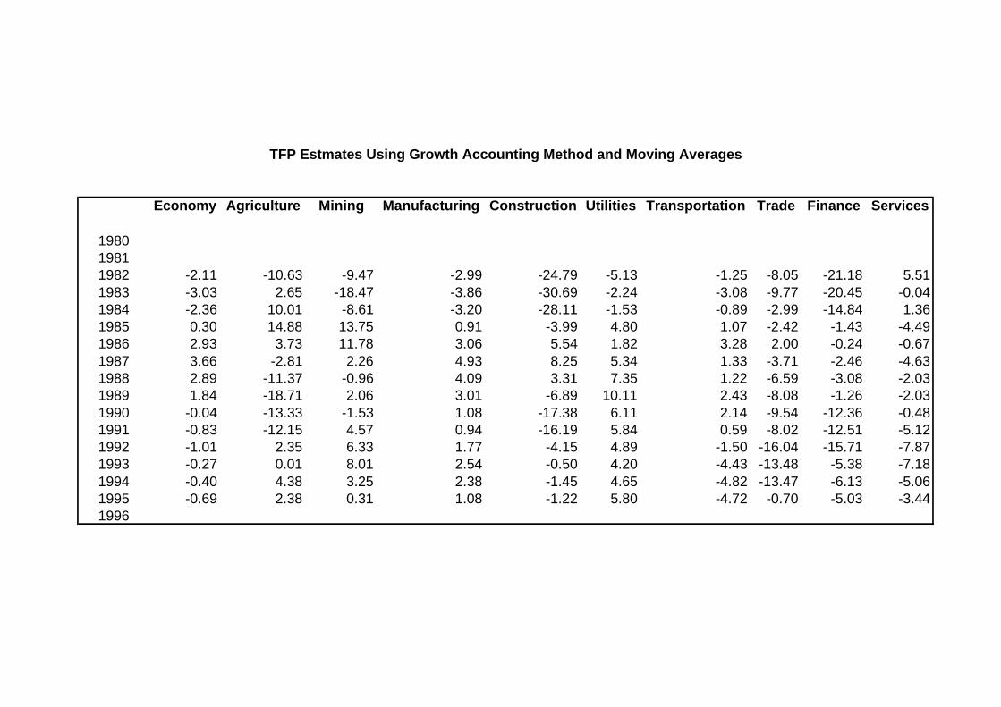
TFP Estmates Using Growth Accounting Method and Moving Averages
Economy Agriculture Mining Manufacturing Construction Utilities Transportation Trade Finance Services
198019811982 -2.11 -10.63 -9.47 -2.99 -24.79 -5.13 -1.25 -8.05 -21.18 5.511983 -3.03 2.65 -18.47 -3.86 -30.69 -2.24 -3.08 -9.77 -20.45 -0.041984 -2.36 10.01 -8.61 -3.20 -28.11 -1.53 -0.89 -2.99 -14.84 1.361985 0.30 14.88 13.75 0.91 -3.99 4.80 1.07 -2.42 -1.43 -4.491986 2.93 3.73 11.78 3.06 5.54 1.82 3.28 2.00 -0.24 -0.671987 3.66 -2.81 2.26 4.93 8.25 5.34 1.33 -3.71 -2.46 -4.631988 2.89 -11.37 -0.96 4.09 3.31 7.35 1.22 -6.59 -3.08 -2.031989 1.84 -18.71 2.06 3.01 -6.89 10.11 2.43 -8.08 -1.26 -2.031990 -0.04 -13.33 -1.53 1.08 -17.38 6.11 2.14 -9.54 -12.36 -0.481991 -0.83 -12.15 4.57 0.94 -16.19 5.84 0.59 -8.02 -12.51 -5.121992 -1.01 2.35 6.33 1.77 -4.15 4.89 -1.50 -16.04 -15.71 -7.871993 -0.27 0.01 8.01 2.54 -0.50 4.20 -4.43 -13.48 -5.38 -7.181994 -0.40 4.38 3.25 2.38 -1.45 4.65 -4.82 -13.47 -6.13 -5.061995 -0.69 2.38 0.31 1.08 -1.22 5.80 -4.72 -0.70 -5.03 -3.441996
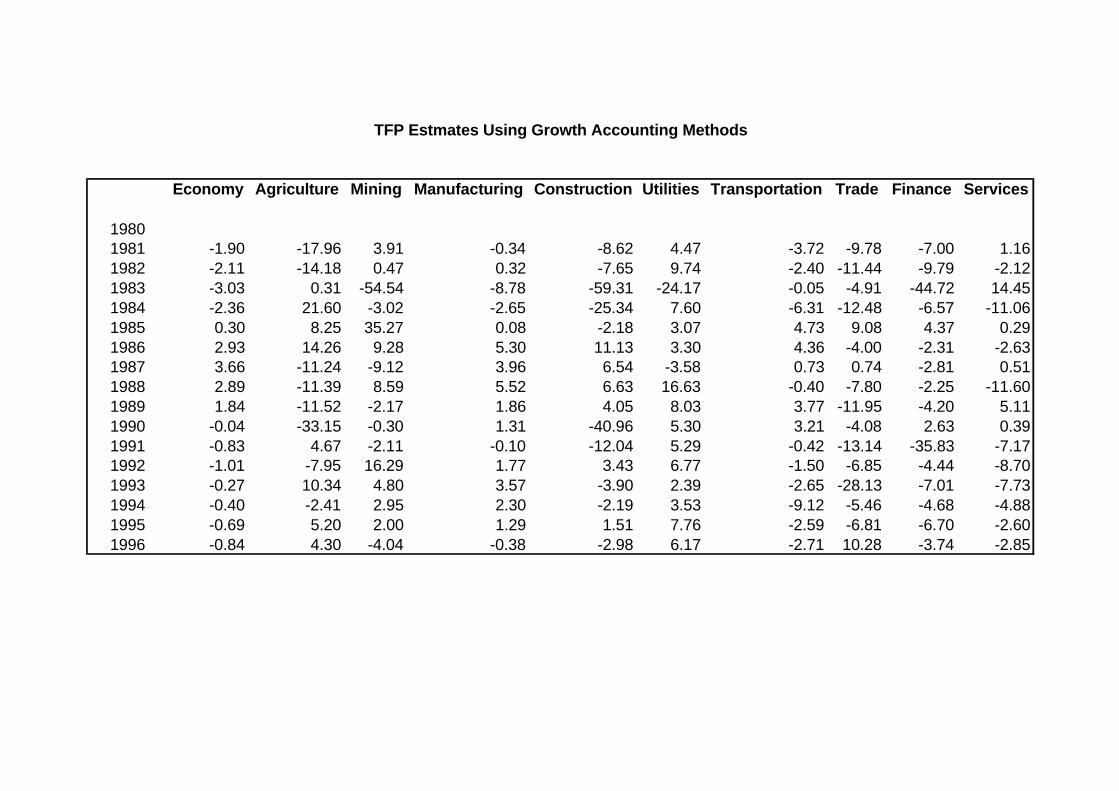
TFP Estmates Using Growth Accounting Methods
Economy Agriculture Mining Manufacturing Construction Utilities Transportation Trade Finance Services
19801981 -1.90 -17.96 3.91 -0.34 -8.62 4.47 -3.72 -9.78 -7.00 1.161982 -2.11 -14.18 0.47 0.32 -7.65 9.74 -2.40 -11.44 -9.79 -2.121983 -3.03 0.31 -54.54 -8.78 -59.31 -24.17 -0.05 -4.91 -44.72 14.451984 -2.36 21.60 -3.02 -2.65 -25.34 7.60 -6.31 -12.48 -6.57 -11.061985 0.30 8.25 35.27 0.08 -2.18 3.07 4.73 9.08 4.37 0.291986 2.93 14.26 9.28 5.30 11.13 3.30 4.36 -4.00 -2.31 -2.631987 3.66 -11.24 -9.12 3.96 6.54 -3.58 0.73 0.74 -2.81 0.511988 2.89 -11.39 8.59 5.52 6.63 16.63 -0.40 -7.80 -2.25 -11.601989 1.84 -11.52 -2.17 1.86 4.05 8.03 3.77 -11.95 -4.20 5.111990 -0.04 -33.15 -0.30 1.31 -40.96 5.30 3.21 -4.08 2.63 0.391991 -0.83 4.67 -2.11 -0.10 -12.04 5.29 -0.42 -13.14 -35.83 -7.171992 -1.01 -7.95 16.29 1.77 3.43 6.77 -1.50 -6.85 -4.44 -8.701993 -0.27 10.34 4.80 3.57 -3.90 2.39 -2.65 -28.13 -7.01 -7.731994 -0.40 -2.41 2.95 2.30 -2.19 3.53 -9.12 -5.46 -4.68 -4.881995 -0.69 5.20 2.00 1.29 1.51 7.76 -2.59 -6.81 -6.70 -2.601996 -0.84 4.30 -4.04 -0.38 -2.98 6.17 -2.71 10.28 -3.74 -2.85

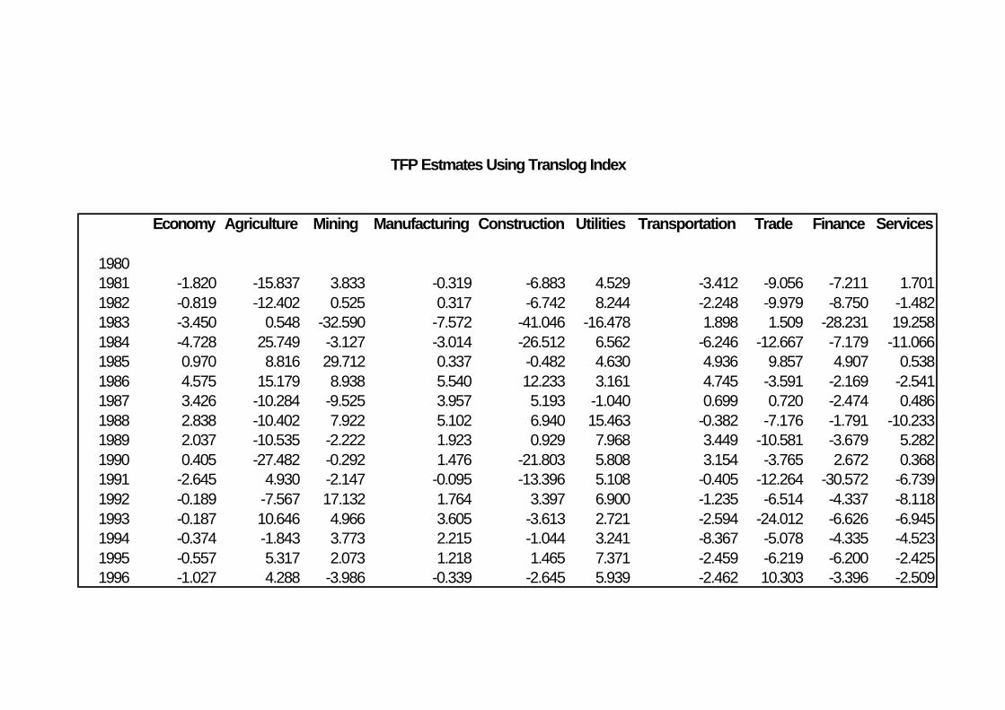
TFP Estmates Using Translog Index
Economy Agriculture Mining Manufacturing Construction Utilities Transportation Trade Finance Services
19801981 -1.820 -15.837 3.833 -0.319 -6.883 4.529 -3.412 -9.056 -7.211 1.7011982 -0.819 -12.402 0.525 0.317 -6.742 8.244 -2.248 -9.979 -8.750 -1.4821983 -3.450 0.548 -32.590 -7.572 -41.046 -16.478 1.898 1.509 -28.231 19.2581984 -4.728 25.749 -3.127 -3.014 -26.512 6.562 -6.246 -12.667 -7.179 -11.0661985 0.970 8.816 29.712 0.337 -0.482 4.630 4.936 9.857 4.907 0.5381986 4.575 15.179 8.938 5.540 12.233 3.161 4.745 -3.591 -2.169 -2.5411987 3.426 -10.284 -9.525 3.957 5.193 -1.040 0.699 0.720 -2.474 0.4861988 2.838 -10.402 7.922 5.102 6.940 15.463 -0.382 -7.176 -1.791 -10.2331989 2.037 -10.535 -2.222 1.923 0.929 7.968 3.449 -10.581 -3.679 5.2821990 0.405 -27.482 -0.292 1.476 -21.803 5.808 3.154 -3.765 2.672 0.3681991 -2.645 4.930 -2.147 -0.095 -13.396 5.108 -0.405 -12.264 -30.572 -6.7391992 -0.189 -7.567 17.132 1.764 3.397 6.900 -1.235 -6.514 -4.337 -8.1181993 -0.187 10.646 4.966 3.605 -3.613 2.721 -2.594 -24.012 -6.626 -6.9451994 -0.374 -1.843 3.773 2.215 -1.044 3.241 -8.367 -5.078 -4.335 -4.5231995 -0.557 5.317 2.073 1.218 1.465 7.371 -2.459 -6.219 -6.200 -2.4251996 -1.027 4.288 -3.986 -0.339 -2.645 5.939 -2.462 10.303 -3.396 -2.509

T a b l e 1 1 : T F P E s t i m a t e s : E c o n o m e t r i c E s t i m a t i o n W i t h o u t i m p o s i n g C R S a s s u m p t i o n o n t h e d a t a( i .e . w i t h o u t i m p o s i n g : a l p h a + b e t a = 1 ) *
U n a d j u s t e d f o r S e r i a l C o r r e l a t i o n
S e c t o r c o n s t a n t a a l p h a b e t a R 2 b a r D W N o . O b s P e r i o d
E c o n o m y - 8 . 9 - 0 . 0 3 4 1 . 4 3 6 0 . 5 9 5 0 . 9 1 8 0 . 9 0 8 1 7 1 9 8 0 - 9 6( t -s ta t ) - 1 . 7 0 1 - 1 . 9 1 2 2 . 6 6 8 5 . 1 3 9
A g r i c u l t u r e 1 0 . 7 4 1 0 . 0 1 1 0 . 0 4 7 0 . 0 8 7 0 . 9 0 9 0 . 8 8 1 1 7 1 9 8 0 - 9 6( t -s ta t ) 2 0 . 1 1 6 5 . 2 0 3 0 . 7 3 4 3 . 3 2 2
M in ing - 7 . 4 4 4 0 . 1 7 9 0 . 2 3 4 1 . 1 9 5 0 . 9 0 3 2 . 1 4 3 1 7 1 9 8 0 - 9 6( t -s ta t ) - 4 . 9 2 6 1 1 . 0 5 1 8 . 1 8 1 0 . 5 0 6
M a n u f a c t u r i n g 0 . 9 3 5 0 . 0 2 7 - 0 . 0 6 4 0 . 8 2 5 0 . 8 9 6 0 . 5 3 9 1 7 1 9 8 0 - 9 6( t -s ta t ) 0 . 3 5 3 6 . 3 8 8 - 0 . 5 9 4 5 . 7 8 1
C o n s t r u c t i o n 6 . 5 8 3 - 0 . 0 5 6 - 0 . 0 2 6 0 . 6 4 9 0 . 6 5 9 0 . 8 4 1 1 7 1 9 8 0 - 9 6( t -s ta t ) 5 . 0 7 7 - 4 . 7 3 4 - 0 . 1 1 7 4 . 9 9 1
Ut i l i t ies - 1 . 3 8 3 0 . 0 7 3 - 0 . 0 2 9 0 . 8 6 7 0 . 9 8 6 0 . 7 6 6 1 7 1 9 8 0 - 9 6( t -s ta t ) - 2 . 1 0 1 2 2 . 1 7 5 - 1 . 5 5 4 1 5 . 9 8 4
T r a n s p o r t a t i o n 7 . 6 9 4 0 . 0 2 1 - 0 . 0 4 4 0 . 2 6 6 0 . 9 4 9 0 . 5 6 2 1 7 1 9 8 0 - 9 6( t -s ta t ) 5 . 6 2 2 4 . 7 0 6 - 0 . 4 1 5 2 . 1 7 7
T r a d e 9 . 2 8 3 0 . 0 1 3 0 . 0 5 1 0 . 1 5 7 0 . 9 5 1 . 4 2 8 1 7 1 9 8 0 - 9 6( t -s ta t ) 1 3 . 3 2 9 1 . 6 6 1 1 . 8 3 2 2 . 0 5
F i n a n c e 7 . 7 2 6 0 . 0 0 5 - 0 . 0 6 8 0 . 3 4 8 0 . 8 7 7 1 . 2 6 1 7 1 9 8 0 - 9 6( t -s ta t ) 5 . 7 9 2 0 . 3 4 4 - 1 . 4 0 7 2 . 9 0 3
S e r v i c e s 8 . 8 8 9 0 . 0 1 1 - 0 . 0 0 4 0 . 2 1 0 . 9 6 4 1 . 0 1 3 1 7 1 9 8 0 - 9 6( t -s ta t ) 9 . 5 7 9 1 . 1 6 8 - 0 . 0 5 7 2 . 6 0 9
A d j u s t e d f o r S e r i a l C o r r e l a t i o n
S e c t o r c o n s t a n t a a l p h a b e t a R 2 b a r D W A R N o . O b s P e r i o d
E c o n o m y - 0 . 9 6 6 - 0 . 0 0 4 0 . 6 2 9 0 . 5 8 0 . 9 5 6 1 . 1 4 2 0 . 6 7 3 1 6 1 9 8 1 - 9 6( t -s ta t ) - 0 . 2 1 6 - 0 . 2 6 1 1 . 5 2 5 2 . 7 5 6 2 . 3 2 3
A g r i c u l t u r e 1 0 . 7 7 2 0 . 0 1 6 0 . 0 8 3 0 . 0 4 4 0 . 9 4 5 2 . 3 6 1 0 . 6 8 1 6 1 9 8 1 - 9 6( t -s ta t ) 2 3 . 4 5 3 2 . 3 7 4 1 . 7 3 3 1 . 0 8 4 2 . 3 9 6
M in ing - 4 . 1 9 0 . 1 2 2 0 . 0 2 5 1 . 0 9 0 . 9 8 6 1 . 8 2 1 0 . 8 6 2 1 6 1 9 8 1 - 9 6( t -s ta t ) - 6 . 0 3 5 7 . 2 3 5 1 . 4 8 3 2 7 . 3 9 3 1 7 . 8 8 9
M a n u f a c t u r i n g 1 . 6 3 0 . 0 2 6 0 . 0 3 2 0 . 7 1 2 0 . 9 4 9 0 . 8 5 9 0 . 7 1 6 1 9 8 1 - 9 6( t -s ta t ) 0 . 5 5 6 4 . 0 5 8 0 . 3 0 5 3 . 3 6 6 2 . 5 0 9
C o n s t r u c t i o n 6 . 0 3 3 - 0 . 0 2 0 . 2 0 5 0 . 4 4 2 0 . 7 9 2 1 . 0 7 6 0 . 7 3 4 1 6 1 9 8 1 - 9 6( t -s ta t ) 5 . 0 0 4 - 0 . 3 2 9 1 . 1 3 7 2 . 5 7 2 . 3 1 8
Ut i l i t ies - 1 . 8 1 9 0 . 0 7 2 - 0 . 0 4 8 0 . 9 1 6 0 . 9 9 1 . 1 8 0 . 8 0 8 1 6 1 9 8 1 - 9 6( t -s ta t ) - 3 . 6 1 5 9 . 0 4 2 - 1 . 9 2 2 6 . 4 1 7 3 . 5 9
T r a n s p o r t a t i o n 6 . 5 0 8 0 . 0 1 8 - 0 . 0 1 6 0 . 3 6 1 0 . 9 6 9 0 . 8 1 3 0 . 7 5 6 1 6 1 9 8 1 - 9 6( t -s ta t ) 4 . 9 7 9 2 . 3 9 8 - 0 . 1 7 3 . 2 4 4 3 . 7 7 1
T r a d e 9 . 4 9 2 0 . 0 1 4 0 . 0 1 7 0 . 1 6 1 0 . 9 4 3 1 . 5 5 6 0 . 4 3 6 1 6 1 9 8 1 - 9 6( t -s ta t ) 9 . 3 8 6 1 . 2 5 3 0 . 4 1 1 . 5 3 6 1 . 3 7 5
F i n a n c e 7 . 3 3 8 0 . 0 0 3 0 . 0 1 1 0 . 3 2 9 1 . 5 2 9 0 . 8 9 7 0 . 5 2 9 1 6 1 9 8 1 - 9 6( t -s ta t ) 4 . 7 4 4 0 . 1 4 4 0 . 1 7 5 1 . 9 8 8 1 . 8 4 2
S e r v i c e s 8 . 7 5 5 0 . 0 1 1 0 . 0 6 5 0 . 1 7 0 . 9 6 5 1 . 6 3 5 0 . 3 6 8 1 6 1 9 8 1 - 9 6( t -s ta t ) 8 . 2 0 9 1 . 0 4 1 0 . 6 2 8 1 . 7 9 1 . 4 1 8* C R S i s c o n s t a n t r e s t u r n s t o s c a l e

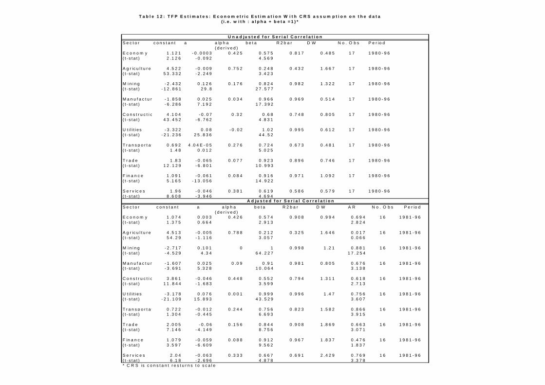
T a b l e 1 2 : T F P E s t i m a t e s : E c o n o m e t r i c E s t i m a t i o n W i t h C R S a s s u m p t i o n o n t h e d a t a( i . e . w i t h : a l p h a + b e t a = 1 ) *
U n a d ju s t e d f o r S e r i a l C o r r e l a t i o n
S e c t o r c o n s t a n t a a lp h a b e t a R 2 b a r D W N o . O b s P e r io d ( d e r i v e d )
E c o n o m y 1 .1 2 1 - 0 . 0 0 0 3 0 .4 2 5 0 .5 7 5 0 .8 1 7 0 .4 8 5 1 7 1 9 8 0 - 9 6( t - s t a t ) 2 .1 2 6 - 0 . 0 9 2 4 .5 6 9
A g r ic u l t u r e 4 .5 2 2 - 0 . 0 0 9 0 .7 5 2 0 .2 4 8 0 .4 3 2 1 .6 6 7 1 7 1 9 8 0 - 9 6( t - s t a t ) 5 3 . 3 3 2 - 2 . 2 4 9 3 .4 2 3
M i n i n g - 2 . 4 3 2 0 .1 2 6 0 .1 7 6 0 .8 2 4 0 .9 8 2 1 .3 2 2 1 7 1 9 8 0 - 9 6( t - s t a t ) - 1 2 . 8 6 1 2 9 . 8 2 7 . 5 7 7
M a n u f a c t u r i n g - 1 . 8 5 8 0 .0 2 5 0 .0 3 4 0 .9 6 6 0 .9 6 9 0 .5 1 4 1 7 1 9 8 0 - 9 6( t - s t a t ) - 6 . 2 8 6 7 .1 9 2 1 7 . 3 9 2
C o n s t r u c t i o n 4 .1 0 4 - 0 . 0 7 0 .3 2 0 .6 8 0 .7 4 8 0 .8 0 5 1 7 1 9 8 0 - 9 6( t - s t a t ) 4 3 . 4 5 2 - 6 . 7 6 2 4 .8 3 1
U t i l i t i e s - 3 . 3 2 2 0 .0 8 - 0 . 0 2 1 .0 2 0 .9 9 5 0 .6 1 2 1 7 1 9 8 0 - 9 6( t - s t a t ) - 2 1 . 2 3 6 2 5 . 8 3 6 4 4 . 5 2
T r a n s p o r t a t i o n 0 .6 9 2 4 .0 4 E - 0 5 0 .2 7 6 0 .7 2 4 0 .6 7 3 0 .4 8 1 1 7 1 9 8 0 - 9 6( t - s t a t ) 1 .4 8 0 .0 1 2 5 .0 2 5
T r a d e 1 .8 3 - 0 . 0 6 5 0 .0 7 7 0 .9 2 3 0 .8 9 6 0 .7 4 6 1 7 1 9 8 0 - 9 6( t - s t a t ) 1 2 . 1 2 9 - 6 . 8 0 1 1 0 . 9 9 3
F in a n c e 1 .0 9 1 - 0 . 0 6 1 0 .0 8 4 0 .9 1 6 0 .9 7 1 1 .0 9 2 1 7 1 9 8 0 - 9 6( t - s t a t ) 5 .1 6 5 - 1 3 . 0 5 6 1 4 . 9 2 2
S e r v ic e s 1 .9 6 - 0 . 0 4 6 0 .3 8 1 0 .6 1 9 0 .5 8 6 0 .5 7 9 1 7 1 9 8 0 - 9 6( t - s t a t ) 8 .6 0 8 - 3 . 9 4 6 4 .6 9 4
A d ju s t e d f o r S e r i a l C o r r e l a t i o n
S e c t o r c o n s t a n t a a lp h a b e t a R 2 b a r D W A R N o . O b s P e r io d ( d e r i v e d )
E c o n o m y 1 .0 7 4 0 .0 0 3 0 .4 2 6 0 .5 7 4 0 .9 0 8 0 .9 9 4 0 .6 9 4 1 6 1 9 8 1 - 9 6( t - s t a t ) 1 .3 7 5 0 .6 6 4 2 .9 1 3 2 .8 2 4
A g r ic u l t u r e 4 .5 1 3 - 0 . 0 0 5 0 .7 8 8 0 .2 1 2 0 .3 2 5 1 .6 4 6 0 .0 1 7 1 6 1 9 8 1 - 9 6( t - s t a t ) 5 4 . 2 9 - 1 . 1 1 6 3 .0 5 7 0 .0 6 6
M i n i n g - 2 . 7 1 7 0 .1 0 1 0 1 0 .9 9 8 1 .2 1 0 .8 8 1 1 6 1 9 8 1 - 9 6( t - s t a t ) - 4 . 5 2 9 4 .3 4 6 4 . 2 2 7 1 7 . 2 5 4
M a n u f a c t u r i n g - 1 . 6 0 7 0 .0 2 5 0 .0 9 0 .9 1 0 .9 8 1 0 .8 0 5 0 .6 7 6 1 6 1 9 8 1 - 9 6( t - s t a t ) - 3 . 6 9 1 5 .3 2 8 1 0 . 0 6 4 3 .1 3 8
C o n s t r u c t i o n 3 .8 6 1 - 0 . 0 4 6 0 .4 4 8 0 .5 5 2 0 .7 9 4 1 .3 1 1 0 .6 1 8 1 6 1 9 8 1 - 9 6( t - s t a t ) 1 1 . 8 4 4 - 1 . 6 8 3 3 .5 9 9 2 .7 1 3
U t i l i t i e s - 3 . 1 7 8 0 .0 7 6 0 .0 0 1 0 .9 9 9 0 .9 9 6 1 .4 7 0 .7 5 6 1 6 1 9 8 1 - 9 6( t - s t a t ) - 2 1 . 1 0 9 1 5 . 8 9 3 4 3 . 5 2 9 3 .6 0 7
T r a n s p o r t a t i o n 0 .7 2 2 - 0 . 0 1 2 0 .2 4 4 0 .7 5 6 0 .8 2 3 1 .5 8 2 0 .8 6 6 1 6 1 9 8 1 - 9 6( t - s t a t ) 1 .3 0 4 - 0 . 4 4 5 6 .6 9 3 3 .9 1 5
T r a d e 2 .0 0 5 - 0 . 0 6 0 .1 5 6 0 .8 4 4 0 .9 0 8 1 .8 6 9 0 .6 6 3 1 6 1 9 8 1 - 9 6( t - s t a t ) 7 .1 4 6 - 4 . 1 4 9 8 .7 5 6 3 .0 7 1
F in a n c e 1 .0 7 9 - 0 . 0 5 9 0 .0 8 8 0 .9 1 2 0 .9 6 7 1 .8 3 7 0 .4 7 6 1 6 1 9 8 1 - 9 6( t - s t a t ) 3 .5 9 7 - 6 . 6 0 9 9 .5 6 2 1 .8 3 7
S e r v ic e s 2 .0 4 - 0 . 0 6 3 0 .3 3 3 0 .6 6 7 0 .6 9 1 2 .4 2 9 0 .7 6 9 1 6 1 9 8 1 - 9 6( t - s t a t ) 6 .1 8 - 2 . 6 9 6 4 .8 7 8 3 .3 7 8* C R S is c o n s t a n t r e s t u r n s t o s c a l e

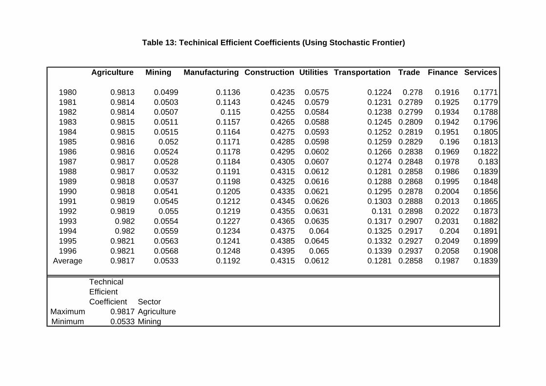
Table 13: Techinical Efficient Coefficients (Using Stochastic Frontier)
Agriculture Mining Manufacturing Construction Utilities Transportation Trade Finance Services
1980 0.9813 0.0499 0.1136 0.4235 0.0575 0.1224 0.278 0.1916 0.17711981 0.9814 0.0503 0.1143 0.4245 0.0579 0.1231 0.2789 0.1925 0.17791982 0.9814 0.0507 0.115 0.4255 0.0584 0.1238 0.2799 0.1934 0.17881983 0.9815 0.0511 0.1157 0.4265 0.0588 0.1245 0.2809 0.1942 0.17961984 0.9815 0.0515 0.1164 0.4275 0.0593 0.1252 0.2819 0.1951 0.18051985 0.9816 0.052 0.1171 0.4285 0.0598 0.1259 0.2829 0.196 0.18131986 0.9816 0.0524 0.1178 0.4295 0.0602 0.1266 0.2838 0.1969 0.18221987 0.9817 0.0528 0.1184 0.4305 0.0607 0.1274 0.2848 0.1978 0.1831988 0.9817 0.0532 0.1191 0.4315 0.0612 0.1281 0.2858 0.1986 0.18391989 0.9818 0.0537 0.1198 0.4325 0.0616 0.1288 0.2868 0.1995 0.18481990 0.9818 0.0541 0.1205 0.4335 0.0621 0.1295 0.2878 0.2004 0.18561991 0.9819 0.0545 0.1212 0.4345 0.0626 0.1303 0.2888 0.2013 0.18651992 0.9819 0.055 0.1219 0.4355 0.0631 0.131 0.2898 0.2022 0.18731993 0.982 0.0554 0.1227 0.4365 0.0635 0.1317 0.2907 0.2031 0.18821994 0.982 0.0559 0.1234 0.4375 0.064 0.1325 0.2917 0.204 0.18911995 0.9821 0.0563 0.1241 0.4385 0.0645 0.1332 0.2927 0.2049 0.18991996 0.9821 0.0568 0.1248 0.4395 0.065 0.1339 0.2937 0.2058 0.1908
Average 0.9817 0.0533 0.1192 0.4315 0.0612 0.1281 0.2858 0.1987 0.1839
TechnicalEfficient Coefficient Sector
Maximum 0.9817 AgricultureMinimum 0.0533 Mining

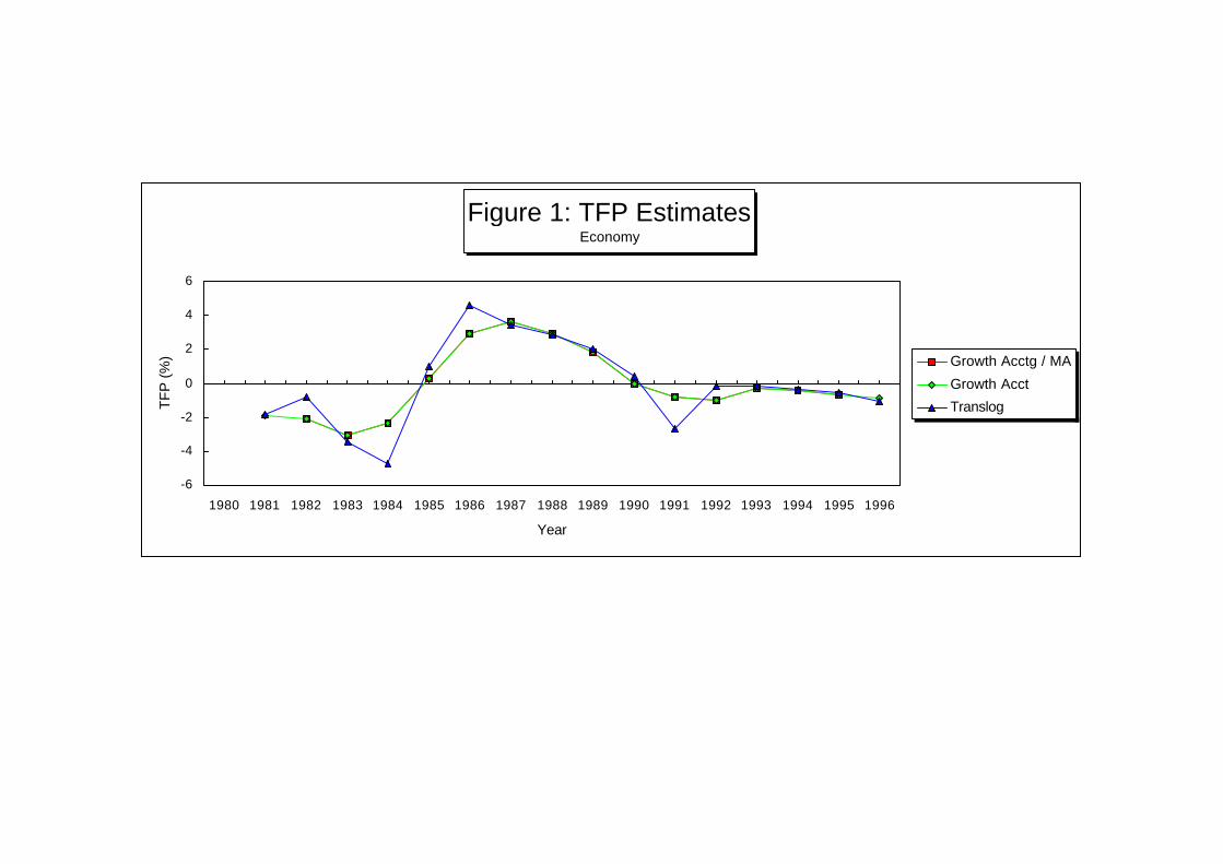
Figure 1: TFP Estimates Economy
-6
-4
-2
0
2
4
6
1980 1981 1982 1983 1984 1985 1986 1987 1988 1989 1990 1991 1992 1993 1994 1995 1996
Year
TF
P (
%) Growth Acctg / MA
Growth Acct
Translog
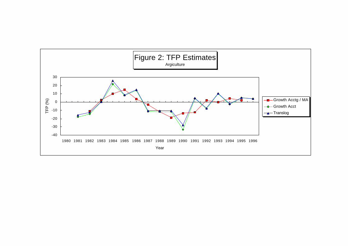
Figure 2: TFP Estimates Argiculture
-40
-30
-20
-10
0
10
20
30
1980 1981 1982 1983 1984 1985 1986 1987 1988 1989 1990 1991 1992 1993 1994 1995 1996
Year
TF
P (
%) Growth Acctg / MA
Growth Acct
Translog
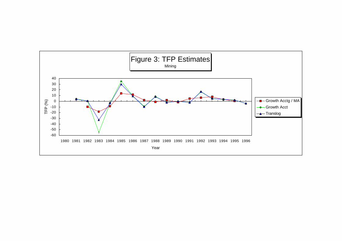
Figure 3: TFP Estimates Mining
-60
-50
-40
-30
-20
-10
0
10
20
30
40
1980 1981 1982 1983 1984 1985 1986 1987 1988 1989 1990 1991 1992 1993 1994 1995 1996
Year
TF
P (
%) Growth Acctg / MA
Growth Acct
Translog
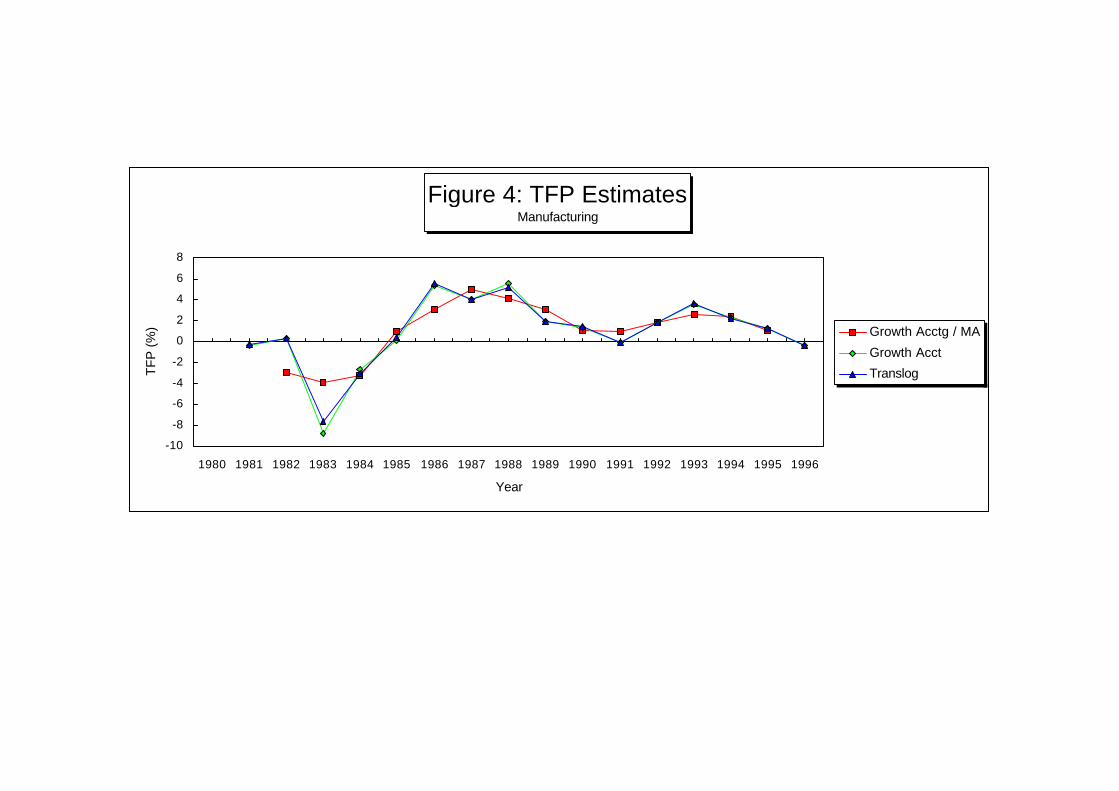
Figure 4: TFP Estimates Manufacturing
-10
-8
-6
-4
-2
0
2
4
6
8
1980 1981 1982 1983 1984 1985 1986 1987 1988 1989 1990 1991 1992 1993 1994 1995 1996
Year
TF
P (
%) Growth Acctg / MA
Growth Acct
Translog
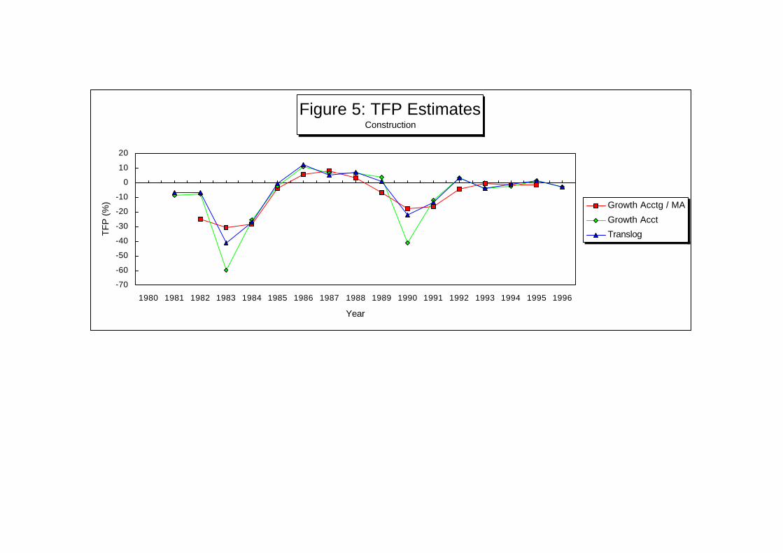
Figure 5: TFP Estimates Construction
-70
-60
-50
-40
-30
-20
-10
0
10
20
1980 1981 1982 1983 1984 1985 1986 1987 1988 1989 1990 1991 1992 1993 1994 1995 1996
Year
TF
P (
%) Growth Acctg / MA
Growth Acct
Translog
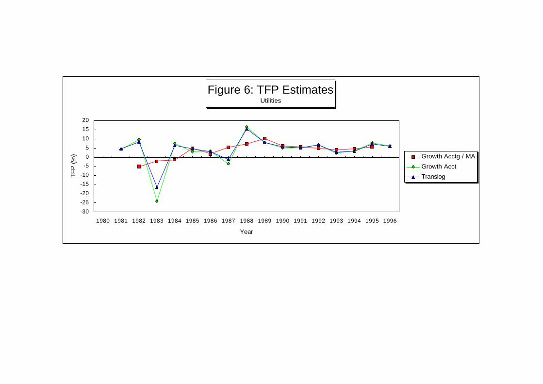
Figure 6: TFP Estimates Utilities
-30
-25
-20
-15
-10
-5
0
5
10
15
20
1980 1981 1982 1983 1984 1985 1986 1987 1988 1989 1990 1991 1992 1993 1994 1995 1996
Year
TF
P (
%) Growth Acctg / MA
Growth Acct
Translog
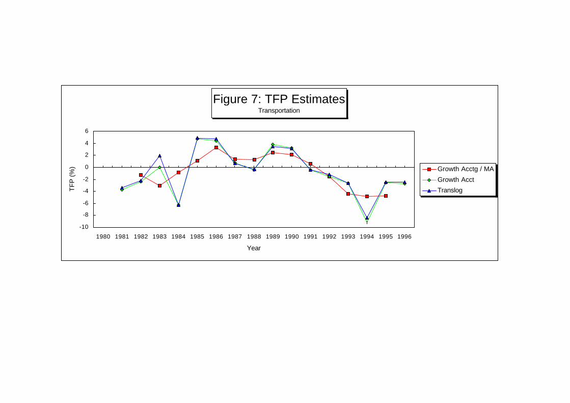
Figure 7: TFP Estimates Transportation
-10
-8
-6
-4
-2
0
2
4
6
1980 1981 1982 1983 1984 1985 1986 1987 1988 1989 1990 1991 1992 1993 1994 1995 1996
Year
TF
P (
%) Growth Acctg / MA
Growth Acct
Translog
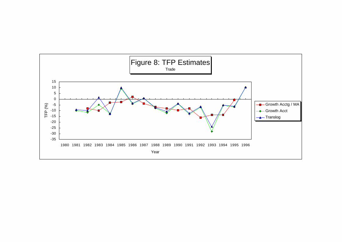
Figure 8: TFP Estimates Trade
-35
-30
-25
-20
-15
-10
-5
0
5
10
15
1980 1981 1982 1983 1984 1985 1986 1987 1988 1989 1990 1991 1992 1993 1994 1995 1996
Year
TF
P (
%) Growth Acctg / MA
Growth Acct
Translog
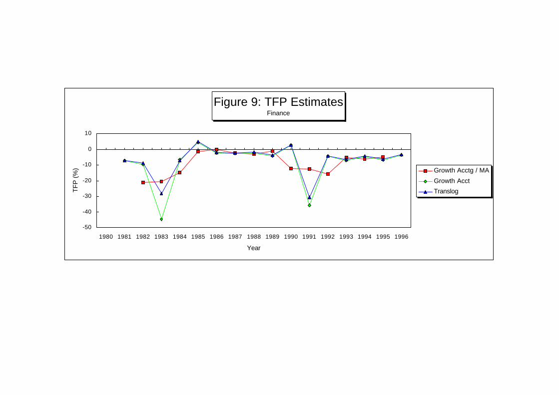
Figure 9: TFP Estimates Finance
-50
-40
-30
-20
-10
0
10
1980 1981 1982 1983 1984 1985 1986 1987 1988 1989 1990 1991 1992 1993 1994 1995 1996
Year
TF
P (
%) Growth Acctg / MA
Growth Acct
Translog
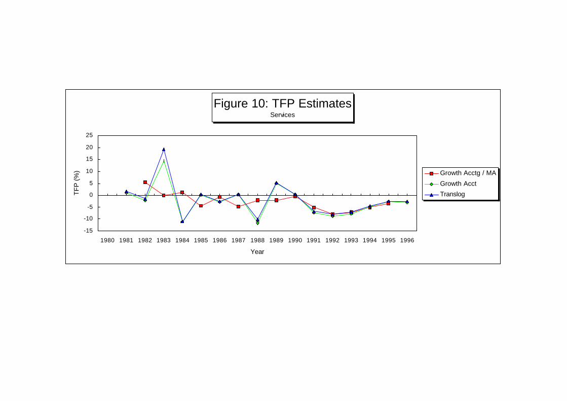
Figure 10: TFP Estimates Services
-15
-10
-5
0
5
10
15
20
25
1980 1981 1982 1983 1984 1985 1986 1987 1988 1989 1990 1991 1992 1993 1994 1995 1996
Year
TF
P (
%) Growth Acctg / MA
Growth Acct
Translog
Appendix A
Methodology Used for ComputingOutput and Factor Inputs
The sector coverage of the Total Factor Productivity (TFP)
estimation in the study includes the entire economy and 9 major sectors. The
9 sectors are (for a detailed description and industry breakdown of these
sectors see Table B1 of Appendix B): (1) agriculture; (2) mining; (3)
manufacturing; (4) construction; (5) utilities; (6) transportation; (7) trade; (8)
finance and dwellings; and (9) services.
The basic strategy adopted by the study was to start the
analysis at the economy level using data from the National Income Accounts
(NIA) and total employment from the Labor Statistics. The reason for doing
this was that both NIA and employment updates come out regularly, and
hence TFP estimates can therefore be updated regularly. The analysis at the
economy level was then brought down to the 9 major sectors listed above
using data from the National Statistics Office (NSO), in particular the Annual
Survey of Establishment (ASE) and other relevant data from the Labor
Statistics. The latter set of data was used to generate distribution shares to
break down data from the NIA and total employment into the major sectors. In
this manner, a consistent set of data is generated from the economy level
using NIA and total employment , and to the major sectors, using the
distribution shares.
NIA-Based Data
The following variables were sourced from the NIA:
1. Total Gross Domestic Products (GDP), sectoral GDP, their
respectively implicit price deflators (IPI), 1985=100.
2. Compensation, total and sectoral
3. Mixed income, total and sectoral
Appendix A—Total Factor Productivity A - 2
4. Net operating surplus, total and sectoral
5. Depreciation, total and sectoral
The complete time series of these variables officially available
covers the period 1980 and 1996. Accordingly, the data base established for
the study covers the same period.
For purposes of TFP estimation, mixed income and net
operating surplus were lumped to form as payment to capital input. Since only
labor and capital were considered as factor inputs in the analysis,
depreciation were deducted from GDP so as to satisfy the accounting identity
that the sum of payment to labor and payment to capital is output (value
added), i.e.,
Q = w*L + r*K
where Q is output (value added), L employment, w wage, K capital, and r rate
of profit.
Both total value added and sectoral value added were deflated
by their respectively 1985 IPI deflators to convert all of them into 1985 prices
(Table A1). The sectoral breakdown of value added into compensation and
surplus is shown in Table A2.
Another important economy level data in the NIA is the Gross
Domestic Capital Formation (hereafter referred to as investments). One of the
biggest problems encountered in the study was how to break down total
investment into sectoral investment. Sectoral investment is important in
deriving the capital stock series in the TFP estimation. A detailed discussion
of the methodology used here is shown in the next few sections.
Appendix A—Total Factor Productivity A - 3
Labor Statistics-Based Data
Total employment was used as indicator of the labor factor
input. In the labor statistics, the longest time series available on sectoral
employment covers only establishments with 10 or more employees. Sectoral
employment data covering all establishments are available only in recent
years, in particular in the 1990s. Thus, to break down total employment into
sectoral employment, the sectoral employment shares covering
establishments with 10 or more employees were applied. The derived
employment series are shown in Table A3.
ASE/NSO-Based Data
As mentioned above, one of the biggest problems encountered
in establishing the data base for the TFP estimation in this study was the
unavailability of sectoral investment. Sectoral investment is relevant in the
estimation of sectoral capital stock series.
There are available information in the ASE though which can be
used to estimate sectoral investment shares, which in turn can be applied to
break down total investment at the economy wide to sectoral investment. One
of the relevant information is the Gross Addition to Fixed Assets (GAFA) at
the sectoral level. However, in the ASE, data on GAFA are not comparable
across sectors because the number of establishments vary across sectors
and through time. To solve this, GAFA data were normalized using
information on the number of establishment. The normalization rule applied is
(Normalized ASE - GAFA data)i t = (GAFAi
t * Ni t )/N t
where Nit is the number of establishments in sector i during period t. These
normalized ASE – GAFA data were used to derive the sectoral investment
shares.
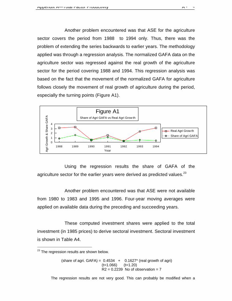
Appendix A—Total Factor Productivity A - 4
Another problem encountered was that ASE for the agriculture
sector covers the period from 1988 to 1994 only. Thus, there was the
problem of extending the series backwards to earlier years. The methodology
applied was through a regression analysis. The normalized GAFA data on the
agriculture sector was regressed against the real growth of the agriculture
sector for the period covering 1988 and 1994. This regression analysis was
based on the fact that the movement of the normalized GAFA for agriculture
follows closely the movement of real growth of agriculture during the period,
especially the turning points (Figure A1).
Using the regression results the share of GAFA of the
agriculture sector for the earlier years were derived as predicted values.23
Another problem encountered was that ASE were not available
from 1980 to 1983 and 1995 and 1996. Four-year moving averages were
applied on available data during the preceding and succeeding years.
These computed investment shares were applied to the total
investment (in 1985 prices) to derive sectoral investment. Sectoral investment
is shown in Table A4.
23 The regression results are shown below.
(share of agri. GAFA) = 0.4534 + 0.1627* (real growth of agri) (t=1.066) (t=1.20) R2 = 0.2239 No of observation = 7
The regression results are not very good. This can probably be modified when a
0
1
2
3
4
YearAgr
i Gro
wth
& S
hare
GA
FA
1988 1989 1990 1991 1992 1993 1994
Real Agri Grow th
Share of Agri GAFA
Figure A1Share of Agri GAFA vs Real Agri Grow th
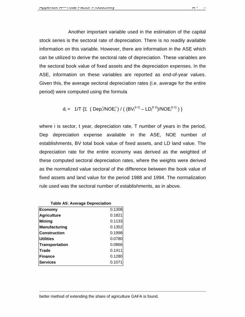
Appendix A—Total Factor Productivity A - 5
Another important variable used in the estimation of the capital
stock series is the sectoral rate of depreciation. There is no readily available
information on this variable. However, there are information in the ASE which
can be utilized to derive the sectoral rate of depreciation. These variables are
the sectoral book value of fixed assets and the depreciation expenses. In the
ASE, information on these variables are reported as end-of-year values.
Given this, the average sectoral depreciation rates (i.e. average for the entire
period) were computed using the formula
di = 1/T Σ ( Depit/NOEi
t ) / ( (BVi[t-1] – LDi
[t-1])/NOEi[t-1] )
where i is sector, t year, depreciation rate, T number of years in the period,
Dep depreciation expense available in the ASE, NOE number of
establishments, BV total book value of fixed assets, and LD land value. The
depreciation rate for the entire economy was derived as the weighted of
these computed sectoral depreciation rates, where the weights were derived
as the normalized value sectoral of the difference between the book value of
fixed assets and land value for the period 1988 and 1994. The normalization
rule used was the sectoral number of establishments, as in above.
Table A5: Average Depreciation
Economy 0.1308
Agriculture 0.1821
Mining 0.1133
Manufacturing 0.1352
Construction 0.1998
Utilities 0.0780
Transportation 0.0866
Trade 0.1411
Finance 0.1280
Services 0.1071
better method of extending the share of agriculture GAFA is found.
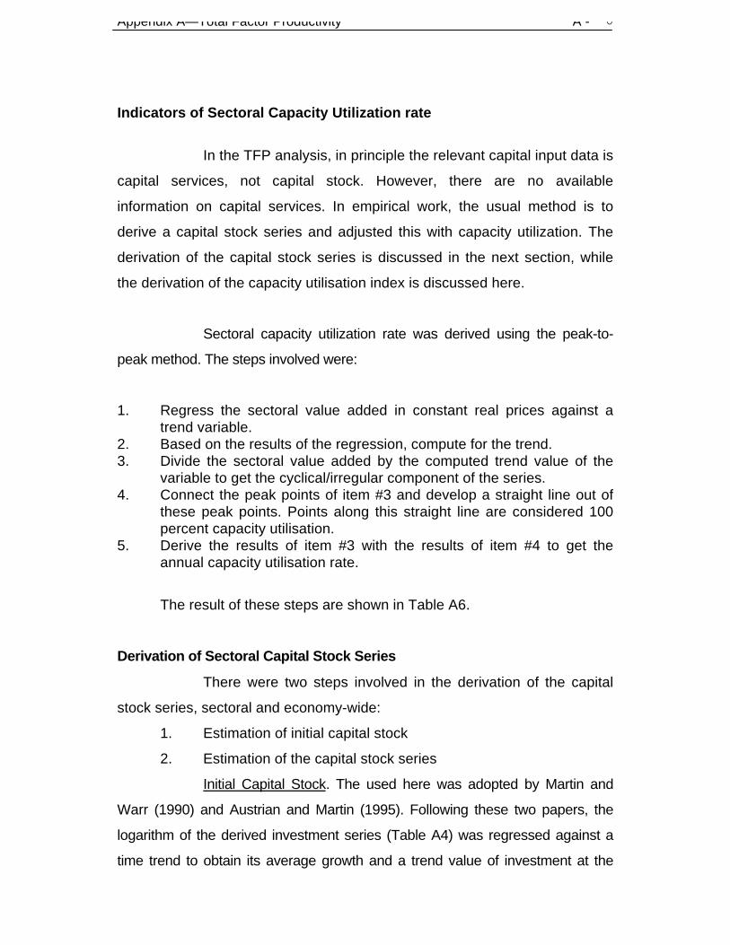
Appendix A—Total Factor Productivity A - 6
Indicators of Sectoral Capacity Utilization rate
In the TFP analysis, in principle the relevant capital input data is
capital services, not capital stock. However, there are no available
information on capital services. In empirical work, the usual method is to
derive a capital stock series and adjusted this with capacity utilization. The
derivation of the capital stock series is discussed in the next section, while
the derivation of the capacity utilisation index is discussed here.
Sectoral capacity utilization rate was derived using the peak-to-
peak method. The steps involved were:
1. Regress the sectoral value added in constant real prices against atrend variable.
2. Based on the results of the regression, compute for the trend.3. Divide the sectoral value added by the computed trend value of the
variable to get the cyclical/irregular component of the series.4. Connect the peak points of item #3 and develop a straight line out of
these peak points. Points along this straight line are considered 100percent capacity utilisation.
5. Derive the results of item #3 with the results of item #4 to get theannual capacity utilisation rate.
The result of these steps are shown in Table A6.
Derivation of Sectoral Capital Stock Series
There were two steps involved in the derivation of the capital
stock series, sectoral and economy-wide:
1. Estimation of initial capital stock
2. Estimation of the capital stock series
Initial Capital Stock. The used here was adopted by Martin and
Warr (1990) and Austrian and Martin (1995). Following these two papers, the
logarithm of the derived investment series (Table A4) was regressed against a
time trend to obtain its average growth and a trend value of investment at the
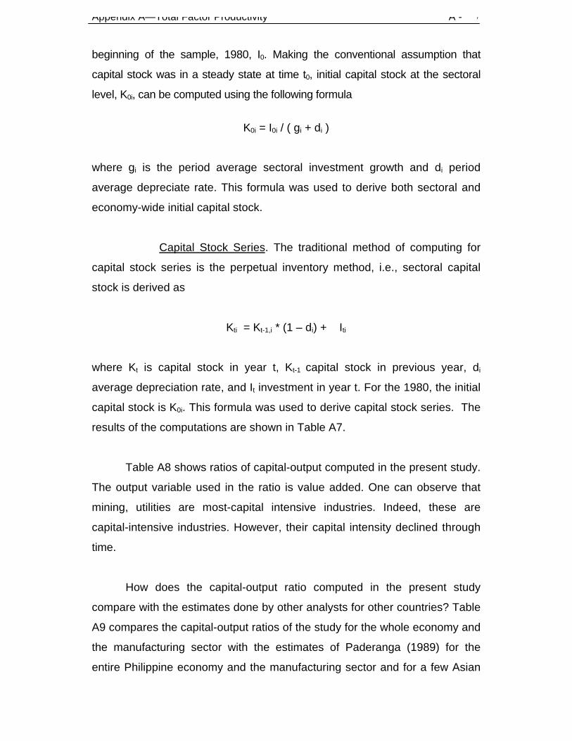
Appendix A—Total Factor Productivity A - 7
beginning of the sample, 1980, I0. Making the conventional assumption that
capital stock was in a steady state at time t0, initial capital stock at the sectoral
level, K0i, can be computed using the following formula
K0i = I0i / ( gi + di )
where gi is the period average sectoral investment growth and di period
average depreciate rate. This formula was used to derive both sectoral and
economy-wide initial capital stock.
Capital Stock Series. The traditional method of computing for
capital stock series is the perpetual inventory method, i.e., sectoral capital
stock is derived as
Kti = Kt-1,i * (1 – di) + Iti
where Kt is capital stock in year t, Kt-1 capital stock in previous year, di
average depreciation rate, and It investment in year t. For the 1980, the initial
capital stock is K0i. This formula was used to derive capital stock series. The
results of the computations are shown in Table A7.
Table A8 shows ratios of capital-output computed in the present study.
The output variable used in the ratio is value added. One can observe that
mining, utilities are most-capital intensive industries. Indeed, these are
capital-intensive industries. However, their capital intensity declined through
time.
How does the capital-output ratio computed in the present study
compare with the estimates done by other analysts for other countries? Table
A9 compares the capital-output ratios of the study for the whole economy and
the manufacturing sector with the estimates of Paderanga (1989) for the
entire Philippine economy and the manufacturing sector and for a few Asian
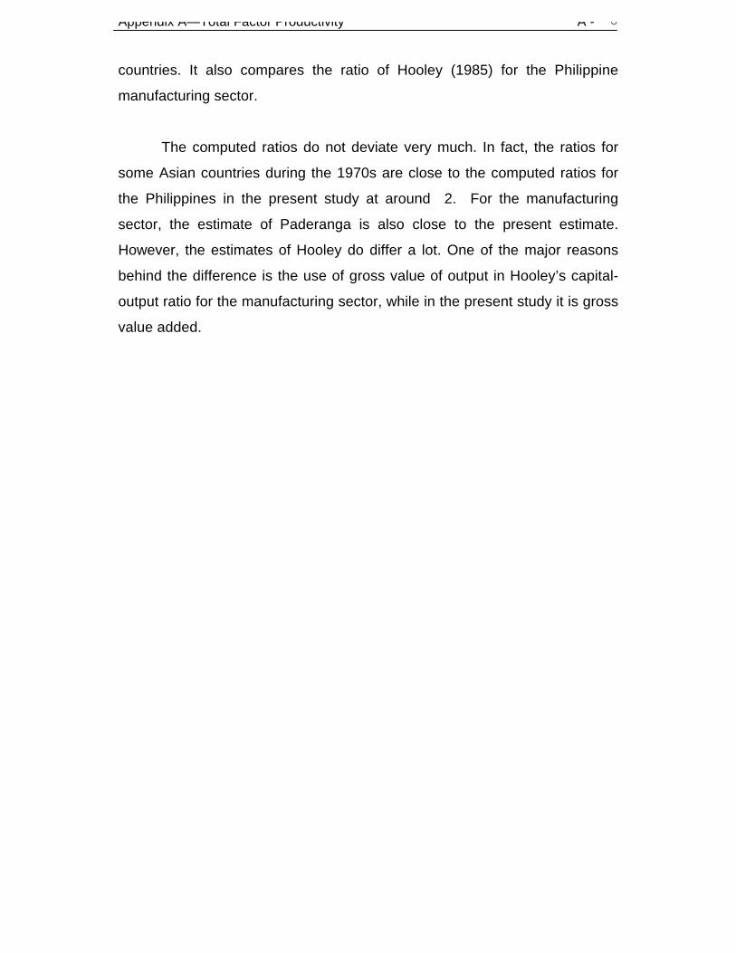
Appendix A—Total Factor Productivity A - 8
countries. It also compares the ratio of Hooley (1985) for the Philippine
manufacturing sector.
The computed ratios do not deviate very much. In fact, the ratios for
some Asian countries during the 1970s are close to the computed ratios for
the Philippines in the present study at around 2. For the manufacturing
sector, the estimate of Paderanga is also close to the present estimate.
However, the estimates of Hooley do differ a lot. One of the major reasons
behind the difference is the use of gross value of output in Hooley’s capital-
output ratio for the manufacturing sector, while in the present study it is gross
value added.

Appendix A—Total Factor Productivity A - 9

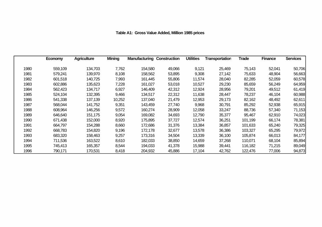
Table A1: Gross Value Added, Million 1985 prices
Economy Agriculture Mining Manufacturing Construction Utilities Transportation Trade Finance Services
1980 559,109 134,703 7,762 154,580 49,066 9,121 25,469 75,143 52,041 50,7061981 579,241 139,970 8,108 158,562 53,895 9,308 27,142 75,633 48,904 56,6631982 601,518 140,725 7,993 161,445 55,806 11,574 28,040 82,285 52,059 60,5781983 602,886 135,623 7,228 161,027 53,018 10,527 29,230 85,659 56,249 64,9591984 562,423 134,717 6,927 146,409 42,312 12,924 28,956 79,201 49,512 61,4191985 524,104 132,395 9,466 134,517 22,312 11,638 28,447 78,237 46,104 60,9881986 541,338 137,139 10,252 137,040 21,479 12,953 29,173 82,162 48,492 62,6111987 568,044 141,752 9,351 143,459 27,740 9,968 30,791 85,292 52,938 65,9151988 608,964 146,256 9,572 160,274 28,909 12,058 33,247 88,736 57,340 71,1531989 646,640 151,175 9,054 169,082 34,693 12,790 35,377 95,467 62,910 74,0231990 671,438 152,000 8,920 175,895 37,727 12,574 36,251 101,199 66,174 78,3811991 664,797 154,288 8,660 172,686 31,376 13,384 36,857 101,633 65,240 79,3251992 668,783 154,820 9,196 172,178 32,677 13,578 36,386 103,327 65,295 79,9721993 683,320 158,463 9,257 173,316 34,504 13,339 36,100 105,874 66,013 84,1771994 711,536 163,522 8,610 182,033 38,850 14,659 37,268 110,071 68,104 85,8941995 745,413 165,357 8,544 194,033 41,378 15,988 39,441 116,182 71,215 89,0491996 790,171 170,531 8,418 204,932 45,886 17,104 42,762 122,476 77,006 94,873
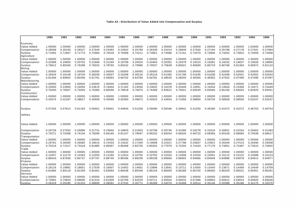
Table A2 : Distribution of Value Added into Compensation and Surplus
1980 1981 1982 1983 1984 1985 1986 1987 1988 1989 1990 1991 1992 1993 1994 1995
EconomyValue-Added 1.00000 1.00000 1.00000 1.00000 1.00000 1.00000 1.00000 1.00000 1.00000 1.00000 1.00000 1.00000 1.00000 1.00000 1.00000 1.00000Compensation 0.28008 0.28193 0.28227 0.27040 0.24482 0.24932 0.25789 0.26339 0.25414 0.28849 0.27930 0.27194 0.26798 0.27178 0.27341 0.27994Surplus 0.71992 0.71807 0.71773 0.72960 0.75518 0.75068 0.74211 0.73661 0.74586 0.71151 0.72070 0.72806 0.73202 0.72822 0.72659 0.72006AgricultureValue-Added 1.00000 1.00000 1.00000 1.00000 1.00000 1.00000 1.00000 1.00000 1.00000 1.00000 1.00000 1.00000 1.00000 1.00000 1.00000 1.00000Compensation 0.20388 0.19655 0.20702 0.21668 0.21240 0.19758 0.20020 0.20463 0.20352 0.19379 0.19310 0.19281 0.19232 0.18637 0.19028 0.18890Surplus 0.79612 0.80345 0.79298 0.78332 0.78760 0.80242 0.79980 0.79537 0.79648 0.80621 0.80690 0.80719 0.80768 0.81363 0.80972 0.81110MiningValue-Added 1.00000 1.00000 1.00000 1.00000 1.00000 1.00000 1.00000 1.00000 1.00000 1.00000 1.00000 1.00000 1.00000 1.00000 1.00000 1.00000Compensation 0.18544 0.19148 0.19704 0.38209 0.40937 0.33298 0.35216 0.35219 0.51465 0.51796 0.51635 0.51638 0.52498 0.52501 0.52502 0.52503Surplus 0.81456 0.80852 0.80296 0.61791 0.59063 0.66702 0.64784 0.64781 0.48535 0.48204 0.48365 0.48362 0.47502 0.47499 0.47498 0.47497ManufacturingValue-Added 1.00000 1.00000 1.00000 1.00000 1.00000 1.00000 1.00000 1.00000 1.00000 1.00000 1.00000 1.00000 1.00000 1.00000 1.00000 1.00000Compensation 0.23550 0.23993 0.24055 0.23615 0.19404 0.21182 0.23030 0.23632 0.16378 0.20449 0.16951 0.16434 0.14834 0.15306 0.15071 0.15449Surplus 0.76450 0.76007 0.75945 0.76385 0.80596 0.78818 0.76970 0.76368 0.83622 0.79551 0.83049 0.83566 0.85166 0.84694 0.84929 0.84551ConstructionValue-Added 1.00000 1.00000 1.00000 1.00000 1.00000 1.00000 1.00000 1.00000 1.00000 1.00000 1.00000 1.00000 1.00000 1.00000 1.00000 1.00000Compensation 0.42674 0.42187 0.38817 0.40599 0.40599 0.55360 0.48672 0.40910 0.43654 0.71059 0.58800 0.59720 0.58928 0.58928 0.53247 0.53247
Surplus 0.57326 0.57813 0.61183 0.59401 0.59401 0.44640 0.51328 0.59090 0.56346 0.28941 0.41200 0.40280 0.41072 0.41072 0.46753 0.46753
Utilities
Value-Added 1.00000 1.00000 1.00000 1.00000 1.00000 1.00000 1.00000 1.00000 1.00000 1.00000 1.00000 1.00000 1.00000 1.00000 1.00000 1.00000
Compensation 0.29729 0.27932 0.25896 0.21731 0.15840 0.18843 0.21903 0.33798 0.30746 0.31580 0.33278 0.31616 0.30841 0.31916 0.29462 0.31383Surplus 0.70271 0.72068 0.74104 0.78269 0.84160 0.81157 0.78097 0.66202 0.69254 0.68420 0.66722 0.68384 0.69159 0.68084 0.70538 0.68617TransportationValue-Added 1.00000 1.00000 1.00000 1.00000 1.00000 1.00000 1.00000 1.00000 1.00000 1.00000 1.00000 1.00000 1.00000 1.00000 1.00000 1.00000Compensation 0.29781 0.28483 0.26582 0.18015 0.14433 0.14532 0.17265 0.19698 0.22021 0.27796 0.25837 0.22821 0.26349 0.27513 0.26490 0.29308Surplus 0.70219 0.71517 0.73418 0.81985 0.85567 0.85468 0.82735 0.80302 0.77979 0.72204 0.74163 0.77179 0.73651 0.72487 0.73510 0.70692TradeValue-Added 1.00000 1.00000 1.00000 1.00000 1.00000 1.00000 1.00000 1.00000 1.00000 1.00000 1.00000 1.00000 1.00000 1.00000 1.00000 1.00000Compensation 0.13457 0.12170 0.14263 0.12203 0.11260 0.11814 0.10792 0.10762 0.10334 0.13308 0.15334 0.15051 0.15112 0.15122 0.15088 0.15123Surplus 0.86543 0.87830 0.85737 0.87797 0.88740 0.88186 0.89208 0.89238 0.89666 0.86692 0.84666 0.84949 0.84888 0.84878 0.84912 0.84877FinanceValue-Added 1.00000 1.00000 1.00000 1.00000 1.00000 1.00000 1.00000 1.00000 1.00000 1.00000 1.00000 1.00000 1.00000 1.00000 1.00000 1.00000Compensation 0.18116 0.19881 0.18651 0.17539 0.16007 0.14452 0.14651 0.13896 0.13941 0.13711 0.14300 0.13440 0.13671 0.14469 0.14549 0.14709Surplus 0.81884 0.80119 0.81349 0.82461 0.83993 0.85548 0.85349 0.86104 0.86059 0.86289 0.85700 0.86560 0.86329 0.85531 0.85451 0.85291ServicesValue-Added 1.00000 1.00000 1.00000 1.00000 1.00000 1.00000 1.00000 1.00000 1.00000 1.00000 1.00000 1.00000 1.00000 1.00000 1.00000 1.00000Compensation 0.73681 0.70820 0.68690 0.61310 0.61909 0.62766 0.64229 0.63711 0.65924 0.66532 0.67486 0.66854 0.65612 0.64814 0.65825 0.66630Surplus 0.26319 0.29180 0.31310 0.38690 0.38091 0.37234 0.35771 0.36289 0.34076 0.33468 0.32514 0.33146 0.34388 0.35186 0.34175 0.33370
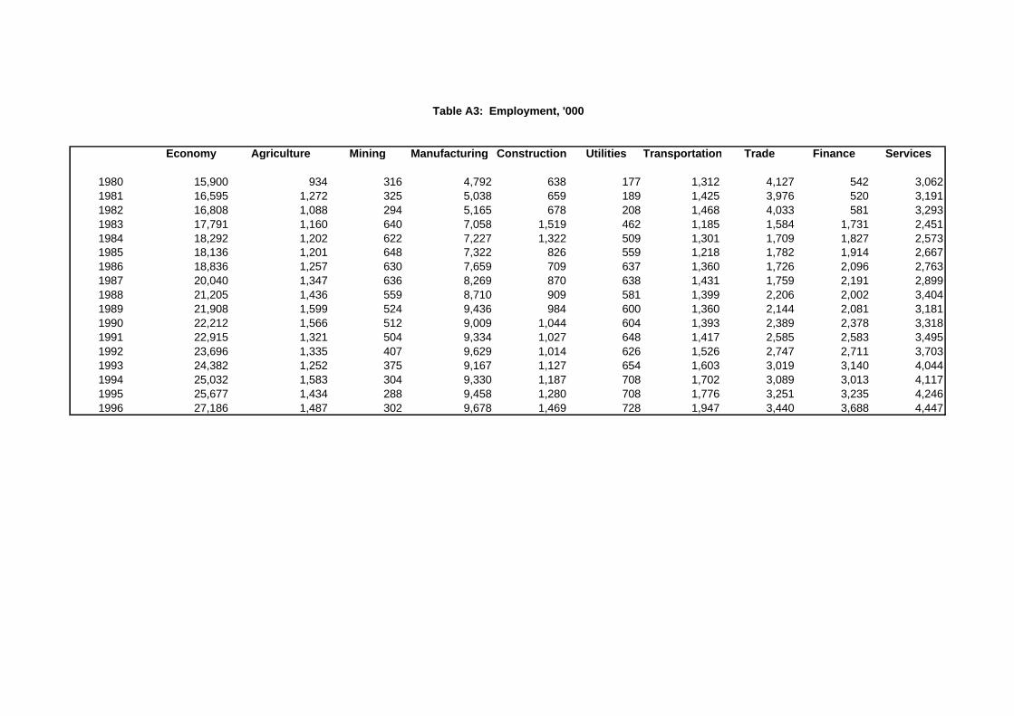
Table A3: Employment, '000
Economy Agriculture Mining Manufacturing Construction Utilities Transportation Trade Finance Services
1980 15,900 934 316 4,792 638 177 1,312 4,127 542 3,0621981 16,595 1,272 325 5,038 659 189 1,425 3,976 520 3,1911982 16,808 1,088 294 5,165 678 208 1,468 4,033 581 3,2931983 17,791 1,160 640 7,058 1,519 462 1,185 1,584 1,731 2,4511984 18,292 1,202 622 7,227 1,322 509 1,301 1,709 1,827 2,5731985 18,136 1,201 648 7,322 826 559 1,218 1,782 1,914 2,6671986 18,836 1,257 630 7,659 709 637 1,360 1,726 2,096 2,7631987 20,040 1,347 636 8,269 870 638 1,431 1,759 2,191 2,8991988 21,205 1,436 559 8,710 909 581 1,399 2,206 2,002 3,4041989 21,908 1,599 524 9,436 984 600 1,360 2,144 2,081 3,1811990 22,212 1,566 512 9,009 1,044 604 1,393 2,389 2,378 3,3181991 22,915 1,321 504 9,334 1,027 648 1,417 2,585 2,583 3,4951992 23,696 1,335 407 9,629 1,014 626 1,526 2,747 2,711 3,7031993 24,382 1,252 375 9,167 1,127 654 1,603 3,019 3,140 4,0441994 25,032 1,583 304 9,330 1,187 708 1,702 3,089 3,013 4,1171995 25,677 1,434 288 9,458 1,280 708 1,776 3,251 3,235 4,2461996 27,186 1,487 302 9,678 1,469 728 1,947 3,440 3,688 4,447
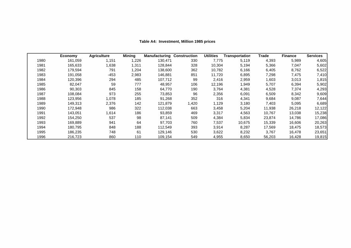
Table A4: Investment, Million 1985 prices
Economy Agriculture Mining Manufacturing Construction Utilities Transportation Trade Finance Services1980 161,059 1,151 1,226 130,471 330 7,775 5,119 4,393 5,989 4,6051981 165,633 1,638 1,311 128,844 328 10,304 5,194 5,366 7,047 5,6021982 179,594 791 1,204 138,600 362 10,782 6,166 6,405 8,762 6,5221983 191,058 -453 2,983 146,881 851 11,720 6,895 7,298 7,475 7,4101984 120,396 294 485 107,712 99 2,416 2,959 1,603 3,013 1,8151985 82,047 59 777 48,957 106 12,196 1,949 5,707 6,394 5,9021986 90,303 845 158 64,770 190 3,764 4,381 4,528 7,374 4,2931987 108,084 973 255 73,853 96 2,356 6,091 6,509 8,342 9,6091988 123,956 1,078 185 91,268 352 316 4,341 9,684 9,087 7,6441989 149,313 2,376 142 121,879 1,420 1,129 3,180 7,403 5,095 6,6891990 172,948 986 322 112,038 663 3,458 5,204 11,938 26,218 12,1221991 143,051 1,614 186 93,859 469 3,317 4,563 10,767 13,038 15,2381992 154,250 537 98 87,141 509 4,384 5,834 23,874 14,786 17,0861993 169,889 941 64 97,703 760 7,537 10,675 15,339 16,606 20,2631994 180,795 848 188 112,549 393 3,914 8,287 17,569 18,475 18,5731995 186,235 748 61 129,146 530 3,622 8,232 3,767 16,478 23,6511996 216,723 860 110 109,154 549 4,955 8,650 56,203 16,428 19,815
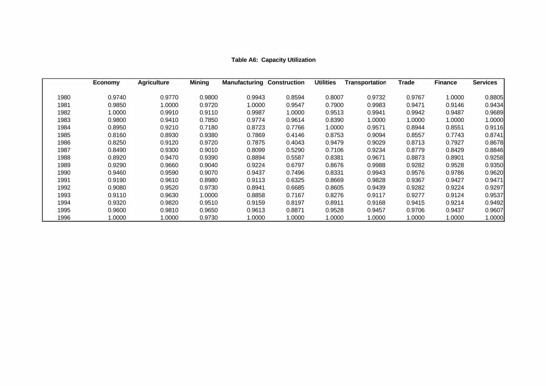
Table A6: Capacity Utilization
Economy Agriculture Mining Manufacturing Construction Utilities Transportation Trade Finance Services
1980 0.9740 0.9770 0.9800 0.9943 0.8594 0.8007 0.9732 0.9767 1.0000 0.88051981 0.9850 1.0000 0.9720 1.0000 0.9547 0.7900 0.9983 0.9471 0.9146 0.94341982 1.0000 0.9910 0.9110 0.9987 1.0000 0.9513 0.9941 0.9942 0.9487 0.96891983 0.9800 0.9410 0.7850 0.9774 0.9614 0.8390 1.0000 1.0000 1.0000 1.00001984 0.8950 0.9210 0.7180 0.8723 0.7766 1.0000 0.9571 0.8944 0.8551 0.91161985 0.8160 0.8930 0.9380 0.7869 0.4146 0.8753 0.9094 0.8557 0.7743 0.87411986 0.8250 0.9120 0.9720 0.7875 0.4043 0.9479 0.9029 0.8713 0.7927 0.86781987 0.8490 0.9300 0.9010 0.8099 0.5290 0.7106 0.9234 0.8779 0.8429 0.88461988 0.8920 0.9470 0.9390 0.8894 0.5587 0.8381 0.9671 0.8873 0.8901 0.92581989 0.9290 0.9660 0.9040 0.9224 0.6797 0.8676 0.9988 0.9282 0.9528 0.93501990 0.9460 0.9590 0.9070 0.9437 0.7496 0.8331 0.9943 0.9576 0.9786 0.96201991 0.9190 0.9610 0.8980 0.9113 0.6325 0.8669 0.9828 0.9367 0.9427 0.94711992 0.9080 0.9520 0.9730 0.8941 0.6685 0.8605 0.9439 0.9282 0.9224 0.92971993 0.9110 0.9630 1.0000 0.8858 0.7167 0.8276 0.9117 0.9277 0.9124 0.95371994 0.9320 0.9820 0.9510 0.9159 0.8197 0.8911 0.9168 0.9415 0.9214 0.94921995 0.9600 0.9810 0.9650 0.9613 0.8871 0.9528 0.9457 0.9706 0.9437 0.96071996 1.0000 1.0000 0.9730 1.0000 1.0000 1.0000 1.0000 1.0000 1.0000 1.0000
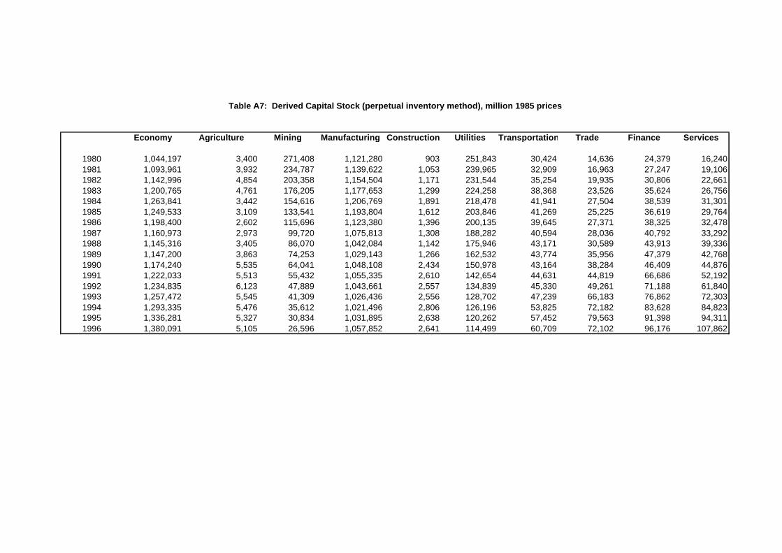
Table A7: Derived Capital Stock (perpetual inventory method), million 1985 prices
Economy Agriculture Mining Manufacturing Construction Utilities Transportation Trade Finance Services
1980 1,044,197 3,400 271,408 1,121,280 903 251,843 30,424 14,636 24,379 16,2401981 1,093,961 3,932 234,787 1,139,622 1,053 239,965 32,909 16,963 27,247 19,1061982 1,142,996 4,854 203,358 1,154,504 1,171 231,544 35,254 19,935 30,806 22,6611983 1,200,765 4,761 176,205 1,177,653 1,299 224,258 38,368 23,526 35,624 26,7561984 1,263,841 3,442 154,616 1,206,769 1,891 218,478 41,941 27,504 38,539 31,3011985 1,249,533 3,109 133,541 1,193,804 1,612 203,846 41,269 25,225 36,619 29,7641986 1,198,400 2,602 115,696 1,123,380 1,396 200,135 39,645 27,371 38,325 32,4781987 1,160,973 2,973 99,720 1,075,813 1,308 188,282 40,594 28,036 40,792 33,2921988 1,145,316 3,405 86,070 1,042,084 1,142 175,946 43,171 30,589 43,913 39,3361989 1,147,200 3,863 74,253 1,029,143 1,266 162,532 43,774 35,956 47,379 42,7681990 1,174,240 5,535 64,041 1,048,108 2,434 150,978 43,164 38,284 46,409 44,8761991 1,222,033 5,513 55,432 1,055,335 2,610 142,654 44,631 44,819 66,686 52,1921992 1,234,835 6,123 47,889 1,043,661 2,557 134,839 45,330 49,261 71,188 61,8401993 1,257,472 5,545 41,309 1,026,436 2,556 128,702 47,239 66,183 76,862 72,3031994 1,293,335 5,476 35,612 1,021,496 2,806 126,196 53,825 72,182 83,628 84,8231995 1,336,281 5,327 30,834 1,031,895 2,638 120,262 57,452 79,563 91,398 94,3111996 1,380,091 5,105 26,596 1,057,852 2,641 114,499 60,709 72,102 96,176 107,862
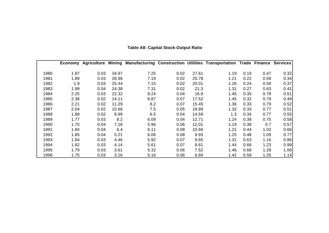
Table A8: Capital Stock-Output Ratio
Economy Agriculture Mining Manufacturing Construction Utilities Transportation Trade Finance Services
1980 1.87 0.03 34.97 7.25 0.02 27.61 1.19 0.19 0.47 0.321981 1.89 0.03 28.96 7.19 0.02 25.78 1.21 0.22 0.56 0.341982 1.9 0.03 25.44 7.15 0.02 20.01 1.26 0.24 0.59 0.371983 1.99 0.04 24.38 7.31 0.02 21.3 1.31 0.27 0.63 0.411984 2.25 0.03 22.32 8.24 0.04 16.9 1.45 0.35 0.78 0.511985 2.38 0.02 14.11 8.87 0.07 17.52 1.45 0.32 0.79 0.491986 2.21 0.02 11.29 8.2 0.07 15.45 1.36 0.33 0.79 0.521987 2.04 0.02 10.66 7.5 0.05 18.89 1.32 0.33 0.77 0.511988 1.88 0.02 8.99 6.5 0.04 14.59 1.3 0.34 0.77 0.551989 1.77 0.03 8.2 6.09 0.04 12.71 1.24 0.38 0.75 0.581990 1.75 0.04 7.18 5.96 0.06 12.01 1.19 0.38 0.7 0.571991 1.84 0.04 6.4 6.11 0.08 10.66 1.21 0.44 1.02 0.661992 1.85 0.04 5.21 6.06 0.08 9.93 1.25 0.48 1.09 0.771993 1.84 0.03 4.46 5.92 0.07 9.65 1.31 0.63 1.16 0.861994 1.82 0.03 4.14 5.61 0.07 8.61 1.44 0.66 1.23 0.991995 1.79 0.03 3.61 5.32 0.06 7.52 1.46 0.68 1.28 1.061996 1.75 0.03 3.16 5.16 0.06 6.69 1.42 0.59 1.25 1.14
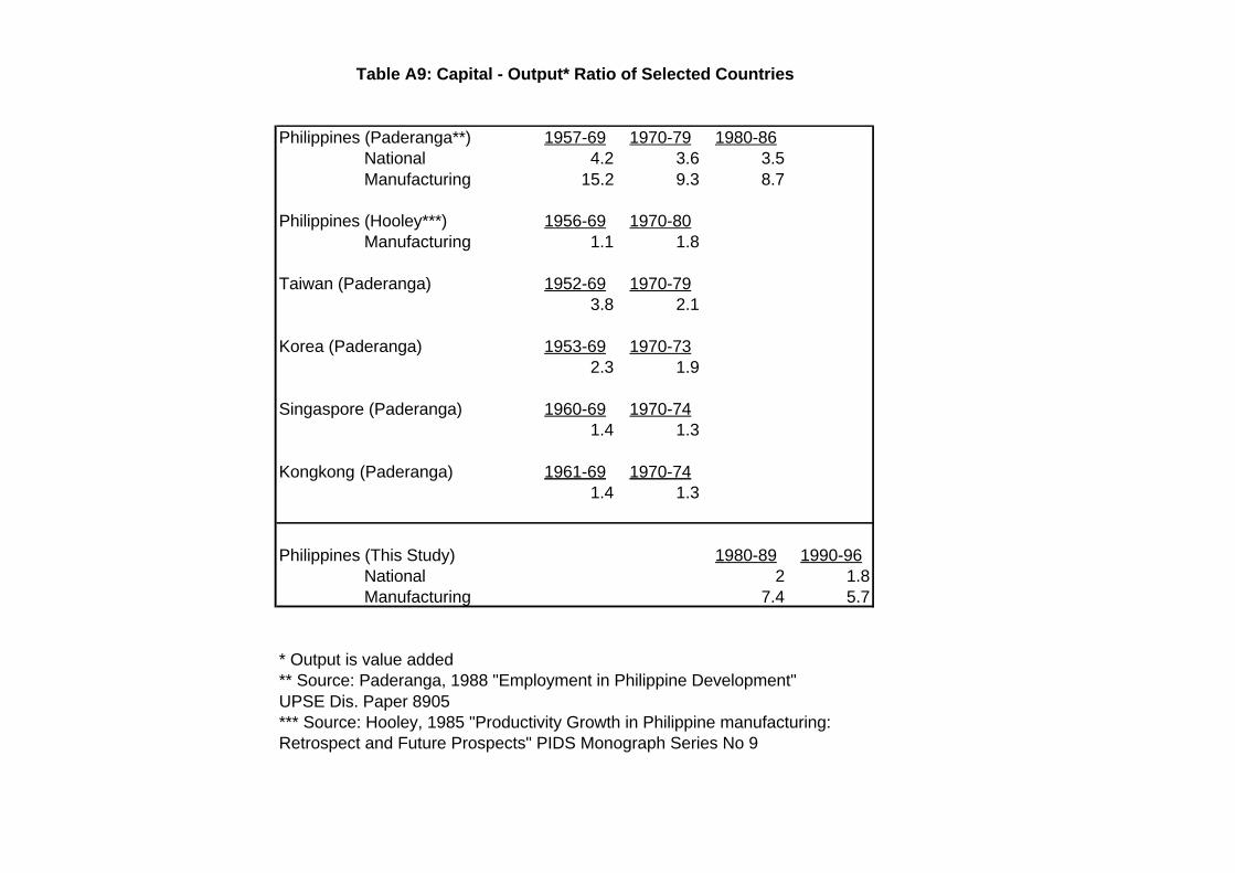
Table A9: Capital - Output* Ratio of Selected Countries
Philippines (Paderanga**) 1957-69 1970-79 1980-86National 4.2 3.6 3.5Manufacturing 15.2 9.3 8.7
Philippines (Hooley***) 1956-69 1970-80Manufacturing 1.1 1.8
Taiwan (Paderanga) 1952-69 1970-793.8 2.1
Korea (Paderanga) 1953-69 1970-732.3 1.9
Singaspore (Paderanga) 1960-69 1970-741.4 1.3
Kongkong (Paderanga) 1961-69 1970-741.4 1.3
Philippines (This Study) 1980-89 1990-96National 2 1.8Manufacturing 7.4 5.7
* Output is value added** Source: Paderanga, 1988 "Employment in Philippine Development" UPSE Dis. Paper 8905*** Source: Hooley, 1985 "Productivity Growth in Philippine manufacturing: Retrospect and Future Prospects" PIDS Monograph Series No 9
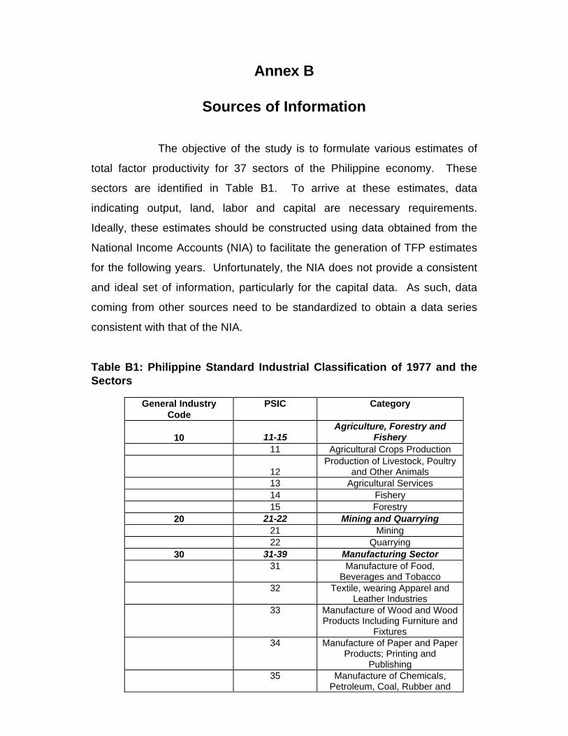
Annex B
Sources of Information
The objective of the study is to formulate various estimates of
total factor productivity for 37 sectors of the Philippine economy. These
sectors are identified in Table B1. To arrive at these estimates, data
indicating output, land, labor and capital are necessary requirements.
Ideally, these estimates should be constructed using data obtained from the
National Income Accounts (NIA) to facilitate the generation of TFP estimates
for the following years. Unfortunately, the NIA does not provide a consistent
and ideal set of information, particularly for the capital data. As such, data
coming from other sources need to be standardized to obtain a data series
consistent with that of the NIA.
Table B1: Philippine Standard Industrial Classification of 1977 and theSectors
General IndustryCode
PSIC Category
10 11-15Agriculture, Forestry and
Fishery11 Agricultural Crops Production
12Production of Livestock, Poultry
and Other Animals13 Agricultural Services14 Fishery15 Forestry
20 21-22 Mining and Quarrying21 Mining22 Quarrying
30 31-39 Manufacturing Sector31 Manufacture of Food,
Beverages and Tobacco32 Textile, wearing Apparel and
Leather Industries33 Manufacture of Wood and Wood
Products Including Furniture andFixtures
34 Manufacture of Paper and PaperProducts; Printing and
Publishing35 Manufacture of Chemicals,
Petroleum, Coal, Rubber and
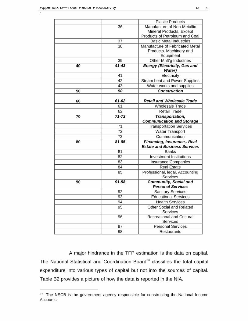
Appendix B—Total Factor Productivity B-
2
Plastic Products36 Manufacture of Non-Metallic
Mineral Products, ExceptProducts of Petroleum and Coal
37 Basic Metal Industries38 Manufacture of Fabricated Metal
Products. Machinery andEquipment
39 Other Mnft’g Industries40 41-43 Energy (Electricity, Gas and
Water)41 Electricity42 Steam heat and Power Supplies43 Water works and supplies
50 50 Construction
60 61-62 Retail and Wholesale Trade61 Wholesale Trade62 Retail Trade
70 71-73 Transportation,Communication and Storage
71 Transportation Services72 Water Transport73 Communication
80 81-85 Financing, Insurance,. RealEstate and Business Services
81 Banks82 Investment Institutions83 Insurance Companies84 Real Estate85 Professional, legal, Accounting
Services90 91-98 Community, Social and
Personal Services92 Sanitary Services93 Educational Services94 Health Services95 Other Social and Related
Services96 Recreational and Cultural
Services97 Personal Services98 Restaurants
A major hindrance in the TFP estimation is the data on capital.
The National Statistical and Coordination Board24 classifies the total capital
expenditure into various types of capital but not into the sources of capital.
Table B2 provides a picture of how the data is reported in the NIA.
24 The NSCB is the government agency responsible for constructing the National IncomeAccounts.
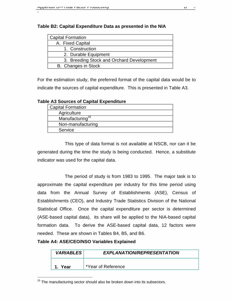
Appendix B—Total Factor Productivity B-
3
Table B2: Capital Expenditure Data as presented in the NIA
Capital Formation A. Fixed Capital 1. Construction 2. Durable Equipment 3. Breeding Stock and Orchard Development
B. Changes in Stock
For the estimation study, the preferred format of the capital data would be to
indicate the sources of capital expenditure. This is presented in Table A3.
Table A3 Sources of Capital ExpenditureCapital Formation Agriculture Manufacturing25
Non-manufacturing Service
This type of data format is not available at NSCB, nor can it be
generated during the time the study is being conducted. Hence, a substitute
indicator was used for the capital data.
The period of study is from 1983 to 1995. The major task is to
approximate the capital expenditure per industry for this time period using
data from the Annual Survey of Establishments (ASE), Census of
Establishments (CEO), and Industry Trade Statistics Division of the National
Statistical Office. Once the capital expenditure per sector is determined
(ASE-based capital data), its share will be applied to the NIA-based capital
formation data. To derive the ASE-based capital data, 12 factors were
needed. These are shown in Tables B4, B5, and B6.
Table A4: ASE/CEO/NSO Variables Explained
VARIABLES EXPLANATION/REPRESENTATION
1. Year *Year of Reference
25 The manufacturing sector should also be broken down into its subsectors.
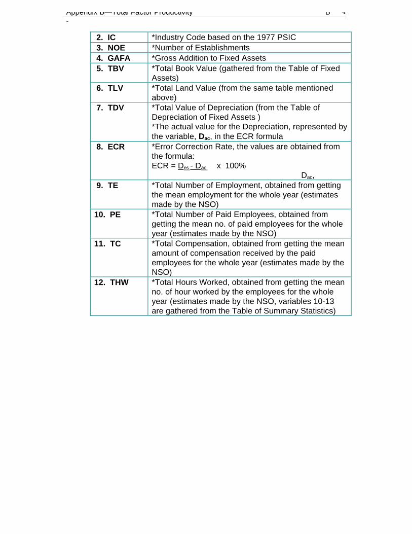
Appendix B—Total Factor Productivity B-
4
2. IC *Industry Code based on the 1977 PSIC 3. NOE *Number of Establishments 4. GAFA *Gross Addition to Fixed Assets 5. TBV *Total Book Value (gathered from the Table of Fixed
Assets) 6. TLV *Total Land Value (from the same table mentioned
above) 7. TDV *Total Value of Depreciation (from the Table of
Depreciation of Fixed Assets )*The actual value for the Depreciation, represented bythe variable, Dac, in the ECR formula
8. ECR *Error Correction Rate, the values are obtained fromthe formula:ECR = Des - Dac x 100% Dac,
9. TE *Total Number of Employment, obtained from gettingthe mean employment for the whole year (estimatesmade by the NSO)
10. PE *Total Number of Paid Employees, obtained fromgetting the mean no. of paid employees for the wholeyear (estimates made by the NSO)
11. TC *Total Compensation, obtained from getting the meanamount of compensation received by the paidemployees for the whole year (estimates made by theNSO)
12. THW *Total Hours Worked, obtained from getting the meanno. of hour worked by the employees for the wholeyear (estimates made by the NSO, variables 10-13are gathered from the Table of Summary Statistics)
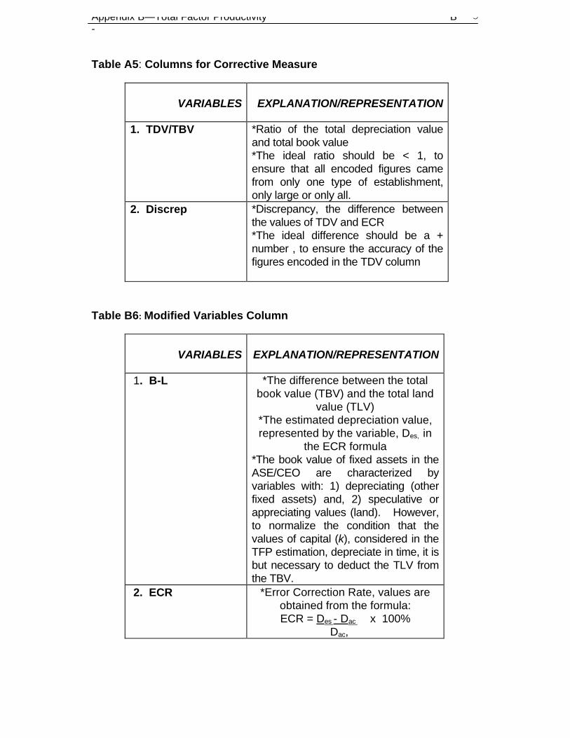
Appendix B—Total Factor Productivity B-
5
Table A5: Columns for Corrective Measure
VARIABLES EXPLANATION/REPRESENTATION
1. TDV/TBV *Ratio of the total depreciation valueand total book value*The ideal ratio should be < 1, toensure that all encoded figures camefrom only one type of establishment,only large or only all.
2. Discrep *Discrepancy, the difference betweenthe values of TDV and ECR*The ideal difference should be a +number , to ensure the accuracy of thefigures encoded in the TDV column
Table B6: Modified Variables Column
VARIABLES EXPLANATION/REPRESENTATION
1. B-L *The difference between the totalbook value (TBV) and the total land
value (TLV)*The estimated depreciation value,represented by the variable, Des, in
the ECR formula*The book value of fixed assets in theASE/CEO are characterized byvariables with: 1) depreciating (otherfixed assets) and, 2) speculative orappreciating values (land). However,to normalize the condition that thevalues of capital (k), considered in theTFP estimation, depreciate in time, it isbut necessary to deduct the TLV fromthe TBV.
2. ECR *Error Correction Rate, values areobtained from the formula:ECR = Des - Dac x 100%
Dac,
Appendix B—Total Factor Productivity B-
6
Considerations, Bias and Selection
Two major deterrents were encountered in the encoding of data; first
was the unavailability of some ASE/CEO/NSO values for some sectors, over
a certain period/s of time; and second was the existence of different table
formats of ASE/CEO/NSO for some sectors, over a certain period of time.
This led to a series of processes before arriving at a single value for a
particular variable. For these reasons, some considerations were made while
validating, reviewing, and processing the obtained figures.
1. From 1983-1987, the ASE/CEO had the same table formats and
bases for computing and determining the values encoded therein.
However, from 1988-1995, the bases were altered, and brought
forth a new table format. From the ASE/CEO 1983-1987, the
presentation was based on the sizes of the establishments, i.e.
large, small or all establishments. Accordingly, these were
determined through the income earnings of the surveyed
establishments. The figures in the ASE/CEO 1988-1995 were
determined according to and on the basis of the average
employment size of these establishments for one year:
establishments with an average employment of ten or more, less
than 10 or 9 and below, or all establishments.
This arrangement led to an inconsistent ASE/CEO figures. For
this matter, the category of industry establishments were placed in a matrix
(please see Matrix, Annex “B”), to finalize which of the values are to be
picked out: large or establishments with employment of 10 or more, or all
establishments. Small establishments or establishments with an average
employment of less than 10, were disregarded based on the opinion that their
contribution to the to the total output is generally negligible..
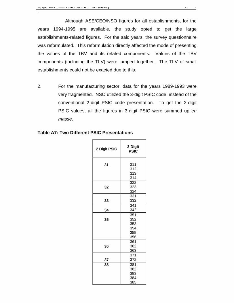
Appendix B—Total Factor Productivity B-
7
Although ASE/CEO/NSO figures for all establishments, for the
years 1994-1995 are available, the study opted to get the large
establishments-related figures. For the said years, the survey questionnaire
was reformulated. This reformulation directly affected the mode of presenting
the values of the TBV and its related components. Values of the TBV
components (including the TLV) were lumped together. The TLV of small
establishments could not be exacted due to this.
2. For the manufacturing sector, data for the years 1989-1993 were
very fragmented. NSO utilized the 3-digit PSIC code, instead of the
conventional 2-digit PSIC code presentation. To get the 2-digit
PSIC values, all the figures in 3-digit PSIC were summed up en
masse.
Table A7: Two Different PSIC Presentations
2 Digit PSIC
3 DigitPSIC
31
311 312 313 314
32
322 323 324
33
331 332
34
341 342
35
351 352 353 354 355 356
36
361 362 363
37
371 372
38 381 382 383 384 385
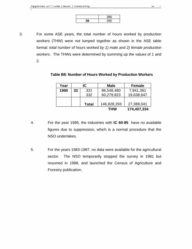
Appendix B—Total Factor Productivity B-
8
386 39 390
3. For some ASE years, the total number of hours worked by production
workers (THW) were not lumped together as shown in the ASE table
format: total number of hours worked by 1) male and 2) female production
workers. The THWs were determined by summing up the values of 1 and
2.
Table B8: Number of Hours Worked by Production Workers
Year IC Male Female 1990 33 331
332 86,548,480 60,279,823
7,941,391 19,638,647
Total
146,828,293
27,388,041 THW 174,407,334
4. For the year 1995, the industries with IC 60-85 have no available
figures due to suppression, which is a normal procedure that the
NSO undertakes.
5. For the years 1983-1987, no data were available for the agricultural
sector. The NSO temporarily stopped the survey in 1981 but
resumed in 1988, and launched the Census of Agriculture and
Forestry publication.

Appendix B—Total Factor Productivity B-
9

Appendix B—Total Factor Productivity B-
10

Appendix B—Total Factor Productivity B-
11