Embed Size (px)
Citation preview
Torus actions and their applications in topology
and combinatorics
Victor M. Buchstaber
Taras E. Panov
Department of Mathematics and Mechanics, Moscow State Univer-sity, 119899 Moscow RUSSIA
E-mail address: [email protected]
Department of Mathematics and Mechanics, Moscow State Univer-sity, 119899 Moscow RUSSIA
E-mail address: [email protected]
1991 Mathematics Subject Classification. 52B70, 57Q15, 57R19, 14M25, 52B05,13F55, 05B35
Key words and phrases. polytopes, simplicial complexes, cubical complexes,Staneley–Reisner rings, torus actions, toric varieties, quasitoric manifolds,
moment-angle complexes, subspace arrangements
Abstract. The aim of this book is to present torus actions as a connectingbridge between combinatorial and convex geometry on one side, and commu-tative and homological algebra, algebraic geometry and topology on the other.The established link helps to understand the geometry and topology of a toricspace by studying the combinatorics of its orbit quotient. Conversely, subtlestproperties of a combinatorial object can be recovered by realizing it as the orbitstructure for a proper manifold or complex acted on by the torus. The lattercan be a symplectic manifold with Hamiltonian torus action, a toric varietyor manifold, a subspace arrangement complement etc., while the combinato-rial objects involved include simplicial and cubical complexes, polytopes andarrangements. Such an approach also provides a natural topological interpre-tation of many constructions from commutative and homological algebra usedin the combinatorics in terms of torus actions.
The exposition centers around the theory of a moment-angle complexes,which provides an effective way to study invariants of triangulations by themethods of equivariant topology. The text is furnished with a large list of bothnew and well-known open problems of relevance to the subject. We hope thatthe book will be useful for topologists as well as combinatorialists and will helpto establish even more tight connections between the subjects involved.
Contents
Introduction 1
Chapter 1. Polytopes 71.1. Definitions and main constructions 71.2. Face vectors and Dehn–Sommerville equations 121.3. The g-theorem 151.4. Upper Bound and Lower Bound theorems 181.5. Stanley–Reisner face rings of simple polytopes 20
Chapter 2. Topology and combinatorics of simplicial complexes 212.1. Abstract simplicial complexes and polyhedrons 212.2. Basic PL topology, and operations with simplicial complexes 232.3. Simplicial spheres 282.4. Triangulated manifolds 292.5. Bistellar moves 31
Chapter 3. Commutative and homological algebra of simplicial complexes 353.1. Stanley–Reisner face rings of simplicial complexes 353.2. Cohen–Macaulay rings and complexes 383.3. Homological algebra background 403.4. Homological properties of face rings: Tor-algebras and Betti numbers 423.5. Gorenstein complexes and Dehn–Sommerville equations 46
Chapter 4. Cubical complexes 494.1. Definitions and cubical maps 494.2. Cubical subdivisions of simple polytopes and simplicial complexes 50
Chapter 5. Toric and quasitoric manifolds 575.1. Toric varieties 575.2. Quasitoric manifolds 635.3. Stably complex structures, and quasitoric representatives in cobordism
classes 695.4. Combinatorial formulae for Hirzebruch genera of quasitoric manifolds 745.5. Classification problems 82
Chapter 6. Moment-angle complexes 856.1. Moment-angle manifolds ZP defined by simple polytopes 856.2. General moment-angle complexes ZK 876.3. Cell decompositions of moment-angle complexes 896.4. Moment-angle complexes corresponding to joins, connected sums and
bistellar moves 92
vii
viii CONTENTS
6.5. Borel constructions and Davis–Januszkiewicz space 946.6. Walk around the construction of ZK : generalizations, analogues and
additional comments 97
Chapter 7. Cohomology of moment-angle complexes and combinatorics oftriangulated manifolds 101
7.1. The Eilenberg–Moore spectral sequence 1017.2. Cohomology algebra of ZK 1027.3. Bigraded Betti numbers of ZK : the case of general K 1067.4. Bigraded Betti numbers of ZK : the case of spherical K 1107.5. Partial quotients of ZP 1137.6. Bigraded Poincare duality and Dehn–Sommerville equations 117
Chapter 8. Cohomology rings of subspace arrangement complements 1258.1. General arrangements and their complements 1258.2. Coordinate subspace arrangements and the cohomology of ZK . 1278.3. Diagonal subspace arrangements and the cohomology of ΩZK . 133
Bibliography 135
Index 141
Introduction
Torus actions on topological spaces is a classical and one of the most developedfields in the equivariant topology. Specific problems connected with torus actionsarise in different areas of mathematics and mathematical physics, which resultsin the permanent interest to the theory, constant source of new applications andpenetration of new ideas in topology. A lot of volumes devoted to particular aspectsof this wide field of mathematical knowledge is available. The topological approachis the subject of monograph [26] by G. Bredon. Monograph [9] by M. Audindeals with torus actions from the symplectic geometry viewpoint. The algebro-geometrical part of the study, known as the geometry of toric varieties or simply“toric geometry”, is presented in several texts. These include original V. Danilov’ssurvey article [46] and more recent monographs by T. Oda [105], W. Fulton [64]and G. Ewald [61].
The orbit space of a torus action carries a reach combinatorial structure. Inmany cases studying the combinatorics of the quotient is the easiest and the most ef-ficient way to understand the topology of a toric space. And this approach works inthe opposite direction as well: the equivariant topology of a torus action sometimeshelps to interpret and prove subtlest combinatorial results topologically. In themost symmetric and regular cases (such as projective toric varieties or Hamiltoniantorus actions on symplectic manifolds) the quotient can be identified with a convexpolytope. More general toric spaces give rise to other combinatorial structures re-lated with their quotients. Examples here include simplicial spheres, triangulatedmanifolds, general simplicial complexes, cubical complexes, subspace arrangementsetc.
Combined applications of combinatorial, topological and algebro-geometricalmethods stimulated intense development of the toric geometry during the lastthree decades. This remarkable confluence of ideas enriched all the subjects in-volved with a number of spectacular results. Another source of applications oftopological and algebraic methods in combinatorics was provided by the theory ofStanley–Reisner face rings and Cohen–Macaulay complexes, described in R. Stan-ley’s monograph [128]. Our motivation was to broaden the existing bridge betweentorus actions and combinatorics by giving some new constructions of toric spaces,which naturally arise from combinatorial considerations. We also interpret manyexisting results in such a way that their relationships with combinatorics becomemore transparent. Traditionally, simplicial complexes, or triangulations, were usedin topology as a tool for combinatorial treatment of topological invariants of spacesor manifolds. On the other hand, triangulations themselves can be regarded asparticular structures, so the space of triangulations becomes the object of study.The idea of considering the space of triangulations of a given manifold has beenalso motivated by some physical problems. One gets an effective way of treatment
1
2 INTRODUCTION
of combinatorial results and problems concerning number of faces in a triangulationby interpreting them as extremal value problems on the space of triangulations. Weimplement some of these ideas in our book as well, by constructing and investigatinginvariants of triangulations using the equivariant topology of toric spaces.
The book is intended to be a systematic but elementary overview for the aspectsof torus actions mostly related to combinatorics. However, our level of expositionis not balanced between topology and combinatorics. We do not assume any par-ticular reader’s knowledge in combinatorics, but in topology a basic knowledge ofcharacteristic classes and spectral sequences techniques may be very helpful in thelast chapters. All necessary information is contained, for instance, in S. Novikov’sbook [104]. We would recommend this volume since it is reasonably concise, hasa rather broad scope and pays much attention to the combinatorial aspects oftopology. Nevertheless, we tried to provide necessary background material in thealgebraic topology and hope that our book will be of interest to combinatorialistsas well.
A significant part of the text is devoted to the theory of moment-angle com-plexes, currently being developed by the authors. This study was inspired bypaper [48] of M. Davis and T. Januszkiewicz, where a topological analogue of toricvarieties was introduced. In their work, Davis and Januszkiewicz used a certainuniversal Tm-space ZK , assigned to every simplicial complex on the vertex set[m] = 1, . . . ,m. In its turn, the definition of ZK was motivated (see [47, §13]) bythe construction of the Coxeter complex of a Coxeter group and its generalizationsby E. Vinberg [137].
Our approach brings the space ZK to the center of attention. To each subsetσ ⊂ [m] there is assigned a canonical Tm-equivariant embedding (D2)k × Tm−k ⊂(D2)m, where (D2)m is the standard poly-disc in Cm and k is the cardinality of σ.This correspondence extends to any simplicial complex K on [m] and produces acanonical bigraded cell decomposition of the Davis–Januszkiewicz Tm-space ZK ,which we refer to as the moment-angle complex . There is also a more general versionof moment-angle complexes, defined for any cubical subcomplex in a unit cube (seesection 4.2). The construction of ZK gives rise to a functor (see Proposition 7.12)from the category of simplicial complexes and inclusions to the category of Tm-spaces and equivariant maps. This functor induces a homomorphism between thestandard simplicial chain complex of a simplicial pair (K1,K2) and the bigradedcellular chain complex of (ZK1 ,ZK2). The remarkable property of the functor isthat it takes a simplicial Lefschetz pair (K1,K2) (i.e. a pair such that K1 \K2 is anopen manifold) to another Lefschetz pair (of moment-angle complexes) in such away that the fundamental cycle is mapped to the fundamental cycle. For instance,if K is a triangulated manifold, then the simplicial pair (K,∅) is mapped to thepair (ZK ,Z∅), where Z∅ ∼= Tm and ZK \ Z∅ is an open manifold. Studying thefunctor K 7→ ZK , one interprets the combinatorics of simplicial complexes in termsof the bigraded cohomology rings of moment-angle complexes. In the case when Kis a triangulated manifold, the important additional information is provided by thebigraded Poincare duality for the Lefschetz pair (ZK ,Z∅). For instance, the dualityimplies the generalized Dehn–Sommerville equations for the numbers of k-simplicesin a triangulated manifold.
INTRODUCTION 3
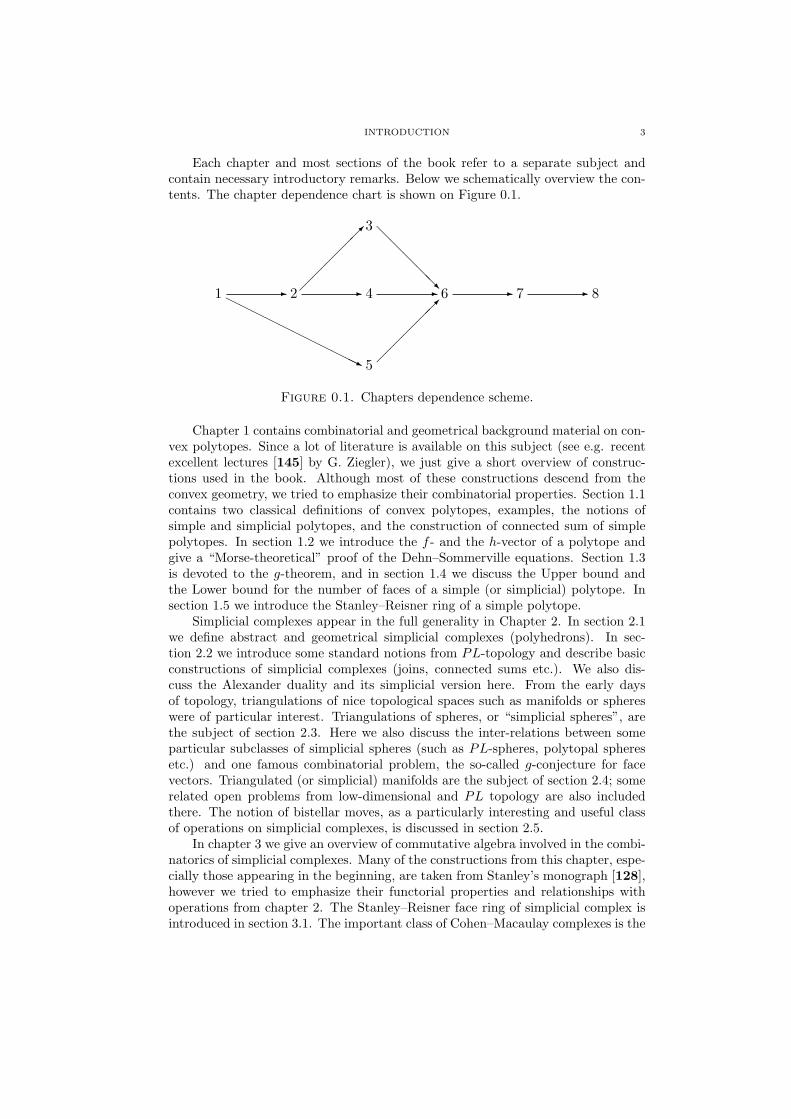
Each chapter and most sections of the book refer to a separate subject andcontain necessary introductory remarks. Below we schematically overview the con-tents. The chapter dependence chart is shown on Figure 0.1.
- - - - -¡¡
¡¡
¡µ
HHHHHHHHHHHj
@@
@@
@R
¡¡
¡¡
¡µ1 2 4 6 7 8
3
5
Figure 0.1. Chapters dependence scheme.
Chapter 1 contains combinatorial and geometrical background material on con-vex polytopes. Since a lot of literature is available on this subject (see e.g. recentexcellent lectures [145] by G. Ziegler), we just give a short overview of construc-tions used in the book. Although most of these constructions descend from theconvex geometry, we tried to emphasize their combinatorial properties. Section 1.1contains two classical definitions of convex polytopes, examples, the notions ofsimple and simplicial polytopes, and the construction of connected sum of simplepolytopes. In section 1.2 we introduce the f - and the h-vector of a polytope andgive a “Morse-theoretical” proof of the Dehn–Sommerville equations. Section 1.3is devoted to the g-theorem, and in section 1.4 we discuss the Upper bound andthe Lower bound for the number of faces of a simple (or simplicial) polytope. Insection 1.5 we introduce the Stanley–Reisner ring of a simple polytope.
Simplicial complexes appear in the full generality in Chapter 2. In section 2.1we define abstract and geometrical simplicial complexes (polyhedrons). In sec-tion 2.2 we introduce some standard notions from PL-topology and describe basicconstructions of simplicial complexes (joins, connected sums etc.). We also dis-cuss the Alexander duality and its simplicial version here. From the early daysof topology, triangulations of nice topological spaces such as manifolds or sphereswere of particular interest. Triangulations of spheres, or “simplicial spheres”, arethe subject of section 2.3. Here we also discuss the inter-relations between someparticular subclasses of simplicial spheres (such as PL-spheres, polytopal spheresetc.) and one famous combinatorial problem, the so-called g-conjecture for facevectors. Triangulated (or simplicial) manifolds are the subject of section 2.4; somerelated open problems from low-dimensional and PL topology are also includedthere. The notion of bistellar moves, as a particularly interesting and useful classof operations on simplicial complexes, is discussed in section 2.5.
In chapter 3 we give an overview of commutative algebra involved in the combi-natorics of simplicial complexes. Many of the constructions from this chapter, espe-cially those appearing in the beginning, are taken from Stanley’s monograph [128],however we tried to emphasize their functorial properties and relationships withoperations from chapter 2. The Stanley–Reisner face ring of simplicial complex isintroduced in section 3.1. The important class of Cohen–Macaulay complexes is the
4 INTRODUCTION
subject of section 3.2; we also give Stanley’s argument for the Upper Bound theo-rem for spheres here. Section 3.3 contains the homological algebra background, in-cluding resolutions and the graded functor Tor. Koszul complexes and Tor-algebrasassociated with simplicial complexes are described in section 3.4 together with theirbasic properties. Gorenstein algebras and Gorenstein* complexes are the subject ofsection 3.5. This class of “self-dual” Cohen–Macaulay complexes contains simplicialand homology spheres and, in a sense, provides the best possible algebraic approx-imation to them. The chapter ends up with a discussion of some generalizations ofthe Dehn–Sommerville equations.
Cubical complexes are the subject of chapter 4. We give definitions and dis-cuss some interesting related problems from the discrete geometry in section 4.1.Section 4.2 introduces some particular cubical complexes necessary for the con-struction of moment-angle complexes. These include the cubical subdivisions ofsimple polytopes and simplicial complexes.
Different aspects of torus actions is the main theme of the second part of thebook. Chapter 5 starts with a brief review of the algebraic geometry of toric va-rieties in section 5.1. We stress upon those features of toric varieties which canbe taken as a starting point for their subsequent topological generalizations. Wealso give famous Stanley’s argument for the necessity part of the g-theorem, oneof the first and most known applications of the algebraic geometry in the combi-natorics of polytopes. In section 5.2 we give the definition and basic propertiesof quasitoric manifolds, the notion introduced by Davis and Januszkiewicz (underthe name “toric manifolds”) as a topological generalization of toric varieties. Thetopology of quasitoric manifolds is the subject of sections 5.3 and 5.4 (this includesthe discussion of their cohomology, cobordisms, characteristic classes, Hirzebruchgenera etc.). Quasitoric manifolds work particularly well in the cobordism theoryand may serve as a convenient framework for different cobordism calculations. Evi-dences for this are provided by some recent results of V. Buchstaber and N. Ray. Itis proved that a certain class of quasitoric manifolds provides an alternative addi-tive basis for the complex cobordism ring. (Note that the standard basis consists ofMilnor hypersurfaces, which are not quasitoric.) Moreover, using the combinatorialconstruction of connected sum of polytopes, it is proved that each complex cobor-dism class contains a quasitoric manifold with a canonical stably almost complexstructure respected by the torus action. Since quasitoric manifolds are necessarilyconnected, the nature of this result resembles the famous Hirzebruch problem aboutconnected algebraic representatives in complex cobordisms. All these arguments,presented in section 5.3, open the way to evaluation of global cobordism invari-ants on manifolds by choosing a quasitoric representative and studying the localinvariants of the action. As an application, in section 5.4 we give combinatorialformulae, due to the second author, for Hirzebruch genera of quasitoric manifolds.Section 5.5 is a discussion of several known results on the classification of toric andquasitoric manifolds over a given simple polytope.
The theory of moment-angle complexes is the subject of chapters 6 and 7. Westart in section 6.1 with the definition of the moment-angle manifold ZP corre-sponding to a simple polytope P . The general moment-angle complexes ZK areintroduced in section 6.2, using special cubical subdivisions from section 4.2. Herewe prove that ZK is a manifold provided that K is a simplicial sphere. Two types
INTRODUCTION 5
of bigraded cell decompositions of moment-angle complexes are introduced in sec-tion 6.3. In section 6.4 we discuss different functorial properties of moment-anglecomplexes with respect to simplicial maps and constructions from section 2.2. Abasic homotopy theory of moment-angle complexes is the subject of section 6.5.Concluding section 6.6 aims for a more broad view on the constructions of qua-sitoric manifolds and moment-angle complexes. We discuss different inter-relations,similar constructions and possible generalizations there.
The cohomology of moment-angle complexes, and its role in investigating com-binatorial invariants of triangulations, is studied in chapter 7. In section 7.1we review the Eilenberg–Moore spectral sequence, our main computational tool.The bigraded cellular structure and the Eilenberg–Moore spectral sequence are themain ingredients in the calculation of cohomology of a general moment-angle com-plex ZK , carried out in section 7.2. Additional results on the cohomology in thecase when K is a simplicial sphere are given in section 7.4. These calculations revealsome new connections with well-known constructions from homological algebra andopen the way to some further combinatorial applications. In particular, the coho-mology of the Koszul complex for a Stanley–Reisner ring and its Betti numbers nowget a topological interpretation. In section 7.5 we study the quotients of moment-angle manifolds ZP by subtori H ⊂ Tm of rank < m. Quasitoric manifolds arisein this scheme as quotients for freely acting subtori of the maximal possible rank.Moment-angle complexes corresponding to triangulated manifolds are consideredin section 7.6. In this situation all singular points of ZK form a single orbit of thetorus action, and the complement of an equivariant neighborhood of this orbit is amanifold with boundary.
In chapter 8 we apply the theory of moment-angle complexes to the topologyof subspace arrangement complements. Section 8.1 is a brief review of general ar-rangements. Then we restrict to the cases of coordinate subspace arrangementsand diagonal subspace arrangements (sections 8.2 and 8.3 respectively). In partic-ular, we calculate the cohomology ring of the complement of a coordinate subspacearrangement by reducing it to the cohomology of a moment-angle complex. Thisalso reveals some remarkable connections between certain results from commutativealgebra of monomial ideals (such as the famous Hochster’s theorem) and topolog-ical results on subspace arrangements (e.g. the Goresky–Macpherson formula forthe cohomology of complement). In the diagonal subspace arrangement case thecohomology of complement includes as a canonical subspace into the cohomologyof the loop space on a certain moment angle complex ZK .
Almost all new concepts in our book are accompanied with explanatory exam-ples. We also give a lot of examples of particular computations, illustrating generaltheorems. Throughout all the text a reader will encounter a number of open prob-lems. Some of these problems and conjectures are widely known, while others arenew. In most cases we tried to give a topological interpretation for the questionunder consideration, which might provide an alternative approach to its solution.
Many of those results in the book which are due to the authors have alreadyappeared in their papers [30]–[34], [111], [112], or papers [37], [38] by N. Ray andthe first author. We sometimes omit the corresponding quotations in the text. Thewhole book has grown up from our survey article [35].
Acknowledgements. Both authors are indebted to Sergey Novikov, whoseinfluence on our topological education can not be overestimated. The first author
6 INTRODUCTION
takes this opportunity to express special thanks to Nigel Ray for the very pleasantjoint work during the last ten years, which in particular generated some of theideas developed in this book. The second author also wishes to express his deepgratitude to N. Ray for extremely fruitful collaboration and sincere hospitalityduring his stay in Manchester. The authors wish to thank Levan Alania, YusufCivan, Natalia Dobrinskaya, Nikolai Dolbilin, Mikhail Farber, Konstantin Feldman,Ivan Izmestiev, Frank Lutz, Oleg Musin, Andrew Ranicki, Elmer Rees, MikhailShtan’ko, Mikhail Shtogrin, Vladimir Smirnov, James Stasheff, Neil Strickland,Sergey Tarasov, Victor Vassiliev, Volkmar Welker, Sergey Yuzvinsky and GunterZiegler for the insight gained from discussions on the subject of our book.
We also thankful to all participants of the seminar “Topology and Compu-tational Geometry”, which is being held by O. R. Musin and the authors at theDepartment of Mathematics and Mechanics, Lomonosov Moscow State University.
We would like to gratefully acknowledge the most helpful comments, correc-tions, and additional references suggested by the referees. Thanks to them, the texthas been significantly enhanced in many places.
The work of both authors was partially supported by the Russian Founda-tion for Fundamental Research, grant no. 99-01-00090, and the Russian LeadingScientific School Support, grant no. 00-15-96011. The second author was also sup-ported by the British Royal Society/NATO Postdoctoral Fellowship while visitingthe Department of Mathematics at the University of Manchester.
CHAPTER 1
Polytopes
1.1. Definitions and main constructions
Both combinatorial and geometrical aspects of the theory of convex polytopesare exposed in a vast number of textbooks, monographs and papers. Amongthem are the classical monograph [69] by Grunbaum and more recent Ziegler’s lec-tures [145]. Face vectors and other combinatorial questions are discussed in booksby McMullen–Shephard [99], Brønsted [29], Yemelichev–Kovalev–Kravtsov [141]and survey article [87] by Klee and Kleinschmidt. These sources contain a host offurther references. In this section we review some basic concepts and constructionsused in the rest of the book.
There are two algorithmically different ways to define a convex polytope inn-dimensional affine Euclidean space Rn.
Definition 1.1. A convex polytope is the convex hull of a finite set of pointsin some Rn.
Definition 1.2. A convex polyhedron P is an intersection of finitely manyhalf-spaces in some Rn:
(1.1) P =x ∈ Rn : 〈l i,x 〉 ≥ −ai, i = 1, . . . , m
,
where l i ∈ (Rn)∗ are some linear functions and ai ∈ R, i = 1, . . . , m. A (convex)polytope is a bounded convex polyhedron.
Nevertheless, the above two definitions produce the same geometrical object,i.e. the subset of Rn is a convex hull of a finite point set if and only if it is abounded intersection of finitely many half-spaces. This classical fact is proved inmany textbooks on polytopes and convex geometry, see e.g. [145, Theorem 1.1].
Definition 1.3. The dimension of a polytope is the dimension of its affinehull. Unless otherwise stated we assume that any n-dimensional polytope, or sim-ply n-polytope, Pn is a subset in n-dimensional ambient space Rn. A supportinghyperplane of Pn is an affine hyperplane H which intersects Pn and for which thepolytope is contained in one of the two closed half-spaces determined by the hyper-plane. The intersection Pn∩H is then called a face of the polytope. We also regardthe polytope Pn itself as a face; other faces are called proper faces. The boundary∂Pn is the union of all proper faces of Pn. Each face of an n-polytope is itself apolytope of dimension ≤ n. 0-dimensional faces are called vertices, 1-dimensionalfaces are edges, and codimension one faces are facets.
Two polytopes P1 ⊂ Rn1 and P2 ⊂ Rn2 of the same dimension are said to beaffinely equivalent (or affinely isomorphic) if there is an affine map Rn1 → Rn2
that is a bijection between the points of the two polytopes. Two polytopes are
7
8 1. POLYTOPES
combinatorially equivalent if there is a bijection between their sets of faces thatpreserves the inclusion relation.
Note that two affinely isomorphic polytopes are combinatorially equivalent, butthe opposite is not true. More consistent definition of combinatorial equivalenceuses the combinatorial notions of poset and lattice.
Definition 1.4. A poset (or finite partially ordered set) (S,≤) is a finite setS equipped with a relation “≤” which is reflexive (x ≤ x for all x ∈ S), transitive(x ≤ y and y ≤ z imply x ≤ z), and antisymmetric (x ≤ y and y ≤ x imply x = y).When the partial order is clear we denote the poset by just S. A chain in S is atotally ordered subset of S.
Definition 1.5. The faces of a polytope P of all dimensions form a poset withrespect to inclusion, called the face poset .
Now we observe that two polytopes are combinatorially equivalent if and onlyif their face posets are isomorphic. More information about face posets of polytopescan be found in [145, §2.2].
Definition 1.6. A combinatorial polytope is a class of combinatorial equivalentconvex (or geometrical) polytopes. Equivalently, a combinatorial polytope is theface poset of a geometrical polytope.
Agreement. Suppose that a polytope Pn is represented as an intersectionof half-spaces as in (1.1). In the sequel we assume that there are no redundantinequalities 〈l i,x 〉 ≥ −ai in such a representation. That is, no inequality can beremoved from (1.1) without changing the polytope Pn. In this case Pn has exactlym facets which are the intersections of hyperplanes 〈l i,x 〉 = −ai, i = 1, . . . , m,with Pn. The vector l i is orthogonal to the corresponding facet and points towardsthe interior of the polytope.
Example 1.7 (simplex and cube). An n-dimensional simplex ∆n is the convexhull of (n + 1) points in Rn that do not lie on a common affine hyperplane. Allfaces of an n-simplex are simplices of dimension ≤ n. Any two n-simplices areaffinely equivalent. The standard n-simplex is the convex hull of points (1, 0, . . . , 0),(0, 1, . . . , 0), . . . , (0, . . . , 0, 1), and (0, . . . , 0) in Rn. Alternatively, the standard n-simplex is defined by (n + 1) inequalities
(1.2) xi ≥ 0, i = 1, . . . , n, and − x1 − . . .− xn ≥ −1.
The regular n-simplex is the convex hull of n + 1 points (1, 0, . . . , 0), (0, 1, . . . , 0),. . ., (0, . . . , 0, 1) in Rn+1.
The standard q-cube is the convex polytope Iq ⊂ Rq defined by
(1.3) Iq = (y1, . . . , yq) ∈ Rq : 0 ≤ yi ≤ 1, i = 1, . . . , q.Alternatively, the standard q-cube is the convex hull of the 2q points in Rq thathave only zero or unit coordinates.
The following construction shows that any convex n-polytope with m facets isaffinely equivalent to the intersection of the positive cone
(1.4) Rm+ =
(y1, . . . , ym) ∈ Rm : yi ≥ 0, i = 1, . . . ,m
⊂ Rm
with a certain n-dimensional plane.
1.1. DEFINITIONS AND MAIN CONSTRUCTIONS 9
Construction 1.8. Let P ⊂ Rn be a convex n-polytope given by (1.1) withsome l i ∈ (Rn)∗, ai ∈ R, i = 1, . . . , m. Form the n ×m-matrix L whose columnsare the vectors l i written in the standard basis of (Rn)∗, i.e. Lji = (l i)j . Note thatL is of rank n. Likewise, let a = (a1, . . . , am)t ∈ Rm be the column vector withentries ai. Then we can rewrite (1.1) as
(1.5) P =x ∈ Rn : (Ltx + a)i ≥ 0, i = 1, . . . , m
,
where Lt is the transposed matrix and x = (x1, . . . , xn)t is the column vector.Consider the affine map
(1.6) AP : Rn → Rm, AP (x ) = Ltx + a ∈ Rm.
Its image is an n-dimensional plane in Rm, and AP (P ) is the intersection of thisplane with the positive cone Rm
+ , see (1.5). Let W be an m× (m−n)-matrix whosecolumns form a basis of linear dependencies between the vectors l i. That is, W isa rank (m− n) matrix satisfying LW = 0. Then it is easy to see that
AP (P ) =y ∈ Rm : W ty = W ta , yi ≥ 0, i = 1, . . . ,m
.
By definition, the polytopes P and AP (P ) are affinely equivalent.
Example 1.9. Consider the standard n-simplex ∆n ⊂ Rn defined by inequali-ties (1.2). It has m = n + 1 facets and is given by (1.1) with l1 = (1, 0, . . . , 0)t, . . .,ln = (0, . . . , 0, 1)t, ln+1 = (−1, . . . ,−1)t, a1 = . . . = an = 0, an+1 = 1. One cantake W = (1, . . . , 1)t in Construction 1.8. Hence, W ty = y1 + . . . + ym, W ta = 1,and we have
A∆n(∆n) =y ∈ Rn+1 : y1 + . . . + yn+1 = 1, yi ≥ 0, i = 1, . . . , n
.
This is the regular n-simplex in Rn+1.
The notion of generic polytope depends on the choice of definition of convexpolytope. Below we describe the two possibilities.
A set of m > n points in Rn is in general position if no (n + 1) of them lie on acommon affine hyperplane. Now Definition 1.1 suggests to call a convex polytopegeneric if it is the convex hull of a set of general positioned points. This impliesthat all proper faces of the polytope are simplices, i.e. every facet has the minimalnumber of vertices (namely, n). Such polytopes are called simplicial .
On the other hand, a set of m > n hyperplanes 〈l i,x 〉 = −ai, l i ∈ (Rn)∗,x ∈ Rn, ai ∈ R, i = 1, . . . , m, is in general position if no point belongs to morethan n hyperplanes. From the viewpoint of Definition 1.2, a convex polytope Pn
is generic if its bounding hyperplanes (see (1.1)) are in general position. That is,there are exactly n facets meeting at each vertex of Pn. Such polytopes are calledsimple. Note that each face of a simple polytope is again a simple polytope.
Definition 1.10. For any convex polytope P ⊂ Rn define its polar set P ∗ ⊂(Rn)∗ by
P ∗ = x ′ ∈ (Rn)∗ : 〈x ′,x 〉 ≥ −1 for all x ∈ P.Remark. We adopt the definition of the polar set from the algebraic geometry
of toric varieties, not the classical one from the convex geometry. The latter isobtained by replacing the inequality “≥ −1” above by “≤ 1”. Obviously, the toricgeometers polar set is taken into the convex geometers one by the central symmetrywith respect to 0.
10 1. POLYTOPES
It is well known in convex geometry that the polar set P ∗ is convex in the dualspace (Rn)∗ and 0 is contained in the interior of P ∗. Moreover, if P itself contains0 in its interior then P ∗ is a convex polytope (i.e. is bounded) and (P ∗)∗ = P ,see e.g. [145, §2.3]. The polytope P ∗ is called the polar (or dual) of P . There isa one-to-one order reversing correspondence between the face posets of P and P ∗.In other words, the face poset of P ∗ is the opposite of the face poset of P . Inparticular, if P is simple then P ∗ is simplicial, and vice versa.
Example 1.11. Any polygon (2-polytope) is simple and simplicial at the sametime. In dimensions ≥ 3 the simplex is the only polytope that is simultaneouslysimple and simplicial. The cube is a simple polytope. The polar of simplex is againthe simplex. The polar of cube is called the cross-polytope. The 3-dimensionalcross-polytope is known as the octahedron.
Construction 1.12 (Product of simple polytopes). The product P1 × P2 oftwo simple polytopes P1 and P2 is a simple polytope as well. The dual operationon simplicial polytopes can be described as follows. Let S1 ⊂ Rn1 and S2 ⊂ Rn2 betwo simplicial polytopes. Suppose that both S1 and S2 contain 0 in their interiors.Now define
S1 S2 := conv(S1 × 0 ∪ 0× S2
) ⊂ Rn1+n2
(here conv means the convex hull). It is easy to see that S1 S2 is a simplicialpolytope, and for any two simple polytopes P1, P2 containing 0 in their interiorsholds
P ∗1 P ∗2 = (P1 × P2)∗.Obviously, both product and operations are also defined on combinatorial poly-topes; in this case the above formula holds without any restrictions.
Construction 1.13 (Connected sum of simple polytopes). Suppose we aregiven two simple polytopes Pn and Qn, both of dimension n, with distinguishedvertices v and w respectively. The informal way to get the connected sum Pn #v,w
Qn of Pn at v and Qn at w is as follows. We “cut off” v from Pn and w from Qn;then, after a projective transformation, we can “glue” the rest of Pn to the rest ofQn along the new simplex facets to obtain Pn #v,w Qn. Below we give the formaldefinition, following [38, §6].
First, we introduce an n-polyhedron Γn, which will be used as a template forthe construction; it arises by considering the standard (n − 1)-simplex ∆n−1 inthe subspace x : x1 = 0 of Rn, and taking its cartesian product with the firstcoordinate axis. The facets Gr of Γn therefore have the form R ×Dr, where Dr,1 ≤ r ≤ n, are the facets of ∆n−1. Both Γn and the Gr are divided into positiveand negative halves, determined by the sign of the coordinate x1.
We order the facets of Pn meeting in v as E1, . . . , En, and the facets of Qn
meeting in w as F1, . . . , Fn. Denote the complementary sets of facets by Cv and Cw;those in Cv avoid v, and those in Cw avoid w.
We now choose projective transformations φP and φQ of Rn, whose purpose isto map v and w to x1 = ±∞ respectively. We insist that φP embeds Pn in Γn
so as to satisfy two conditions; firstly, that the hyperplane defining Er is identifiedwith the hyperplane defining Gr, for each 1 ≤ r ≤ n, and secondly, that theimages of the hyperplanes defining Cv meet Γn in its negative half. Similarly, φQ
identifies the hyperplane defining Fr with that defining Gr, for each 1 ≤ r ≤ n,but the images of the hyperplanes defining Cw meet Γn in its positive half. We
1.1. DEFINITIONS AND MAIN CONSTRUCTIONS 11
define the connected sum Pn #v,w Qn of Pn at v and Qn at w to be the simpleconvex n-polytope determined by the images of the hyperplanes defining Cv and Cw
and hyperplanes defining Gr, r = 1, . . . , n. It is defined only up to combinatorialequivalence; moreover, different choices for either of v and w, or either of theorderings for Er and Fr, are likely to affect the combinatorial type. When thechoices are clear, or their effect on the result irrelevant, we use the abbreviationPn # Qn.
The related construction of connected sum P # S of a simple polytope P anda simplicial polytope S is described in [145, Example 8.41].
Example 1.14. 1. If P 2 is an m1-gon and Q2 is an m2-gon then P # Q is an(m1 + m2 − 2)-gon.
2. If both P and Q are n-simplices then P # Q = ∆n−1 × I1 (the product of(n− 1)-simplex and segment). In particular, for n = 3 we get a triangular prism.
3. More generally, if P is an n-simplex then P #v,w Q is the result of “cutting”the vertex w from Q by a hyperplane that isolate w from other vertices. For morerelations between connected sums and hyperplane cuts see [38, §6].
Definition 1.15. A simplicial polytope S is called k-neighborly if any k verticesspan a face of S. Likewise, a simple polytope P is called k-neighborly if anyk facets of P have non-empty intersection (i.e. share a common codimension-kface). Obviously, every simplicial (or simple) polytope is 1-neighborly. It canbe shown ([29, Corollary 14.5], see also Example 1.24 below) that if S is a k-neighborly simplicial n-polytope and k >
[n2
], then S is an n-simplex. This implies
that any 2-neighborly simplicial 3-polytope is a simplex. However, there existsimplicial n-polytopes with arbitrary number of vertices which are
[n2
]-neighborly.
Such polytopes are called neighborly . In particular, there is a simplicial 4-polytope(different from the 4-simplex) any two vertexes of which are connected by an edge.
Example 1.16 (neighborly 4-polytope). Let P = ∆2 ×∆2 be the product oftwo triangles. Then P is a simple polytope, and it is easy to see that any twofacets of P share a common 2-face. Hence, P is 2-neighborly. The polar P ∗ is aneighborly simplicial 4-polytope.
More generally, if a simple polytope P1 is k1-neighborly and a simple polytopeP2 is k2-neighborly, then the product P1 × P2 is a min(k1, k2)-neighborly simplepolytope. It follows that (∆n × ∆n)∗ and (∆n × ∆n+1)∗ provide examples ofneighborly simplicial 2n- and (2n + 1)-polytopes. The following example gives aneighborly polytope with arbitrary number of vertices.
Example 1.17 (cyclic polytopes). Define the moment curve in Rn by
x : R −→ Rn, t 7→ x (t) = (t, t2, . . . , tn) ∈ Rn.
For any m > n define the cyclic polytope Cn(t1, . . . , tm) as the convex hull of mdistinct points x (ti), t1 < t2 < . . . < tm, on the moment curve. It follows fromthe Vandermonde determinant identity that no (n+1) points on the moment curvebelong to a common affine hyperplane. Hence, Cn(t1, . . . , tm) is a simplicial n-polytope. It can be shown (see [145, Theorem 0.7]) that Cn(t1, . . . , tm) has exactlym vertices x (ti), the combinatorial type of cyclic polytope does not depend onthe specific choice of the parameters t1, . . . , tm, and Cn(t1, . . . , tm) is a neighborlysimplicial n-polytope. We will denote the combinatorial cyclic n-polytope with mvertices by Cn(m).
12 1. POLYTOPES
1.2. Face vectors and Dehn–Sommerville equations
The notion of the f -vector (or face vector) is a central concept in the combi-natorial theory of polytopes. It has been studied there since the time of Euler.
Definition 1.18. Let S be a simplicial n-polytope. Denote by fi the numberof i-dimensional faces of S. The integer vector f (S) = (f0, . . . , fn−1) is called thef -vector of S. We also put f−1 = 1. The h-vector of S is the integer vector(h0, h1, . . . , hn) defined from the equation
(1.7) h0tn + . . . + hn−1t + hn = (t− 1)n + f0(t− 1)n−1 + . . . + fn−1.
Finally, the sequence (g0, g1, . . . , g[n2
]) where g0 = 1, gi = hi−hi−1, i > 0, is called
the g-vector of S.The f -vector of a simple n-polytope Pn is defined as the f -vector of its polar:
f (P ) := f (P ∗), and similarly for the h- and the g-vector of P . More explicitly,f (P ) = (f0, . . . , fn−1), where fi is the number of faces of P of codimension (i + 1)(i.e. of dimension (n− i− 1)). In particular, f0 is the number of facets of P , whichwe usually denote m(P ) or just m. The agreement f−1 = 1 is now justified by thefact that P itself is a face of codimension 0.
Remark. The definition of h-vector may seem to be unnatural at the firstglance. However, as we will see later, the h-vector has a number of combinatorial-geometrical and algebraic interpretations and in some situations is more convenientto work with than the f -vector.
Obviously, the f -vector is a combinatorial invariant of Pn, that is, it dependsonly on the face poset. For convenience we assume all polytopes in this section tobe combinatorial, unless otherwise stated.
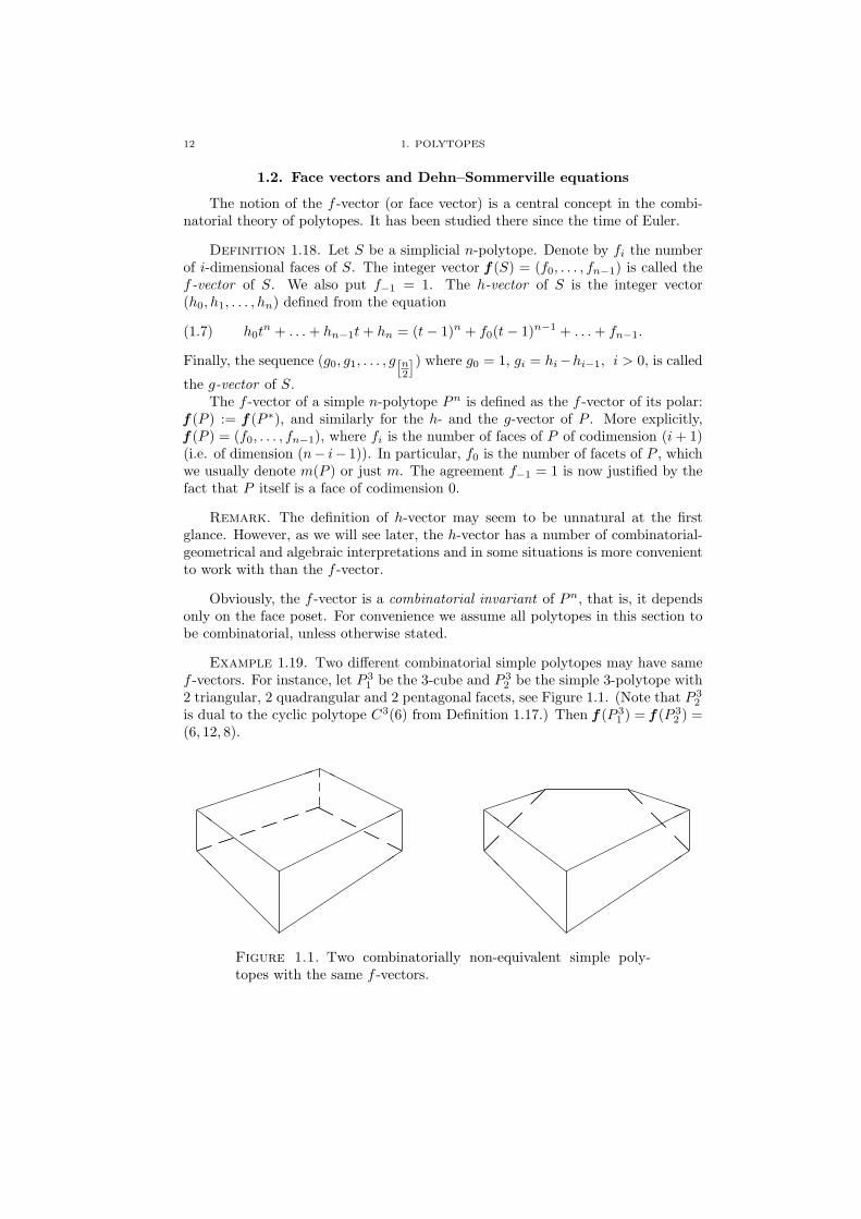
Example 1.19. Two different combinatorial simple polytopes may have samef -vectors. For instance, let P 3
1 be the 3-cube and P 32 be the simple 3-polytope with
2 triangular, 2 quadrangular and 2 pentagonal facets, see Figure 1.1. (Note that P 32
is dual to the cyclic polytope C3(6) from Definition 1.17.) Then f (P 31 ) = f (P 3
2 ) =(6, 12, 8).
@@
@@
@@
´´
´´
´´
´´
³³³³³³³³³
HHHHHH
ZZ
ZZ
ZZ
©©©©©©©©©
³³ ³³ ³³ ³³ ³³ ³³
HHHH
HHHH
@@
@@
@@
´´
´´
´´
´´
³³³³³ PPPPP
ZZ
ZZ
ZZ
©©©©©©©©©
¡¡
¡¡
¡¡
@@
@@
@@
Figure 1.1. Two combinatorially non-equivalent simple poly-topes with the same f -vectors.
1.2. FACE VECTORS AND DEHN–SOMMERVILLE EQUATIONS 13
The f -vector and the h-vector carry the same information about the polytopeand determine each other by means of linear relations, namely
(1.8) hk =k∑
i=0
(−1)k−i(
n−in−k
)fi−1, fn−1−k =
n∑
q=k
(qk
)hn−q, k = 0, . . . , n.
In particular, h0 = 1 and hn = (−1)n(1− f0 + f1 + . . . + (−1)nfn−1
). By Euler’s
theorem,
(1.9) f0 − f1 + · · ·+ (−1)n−1fn−1 = 1 + (−1)n−1,
which is equivalent to hn = h0(= 1). In the case of simple polytopes Euler’stheorem admits the following generalization.
Theorem 1.20 (Dehn–Sommerville relations). The h-vector of any simple orsimplicial n-polytope is symmetric, i.e.
hi = hn−i, i = 0, 1, . . . , n.
The Dehn–Sommerville equations can be proved in a lot of different ways. Wegive a proof which uses a Morse-theoretical argument, firstly appeared in [29]. Wewill return to this argument in chapter 5.
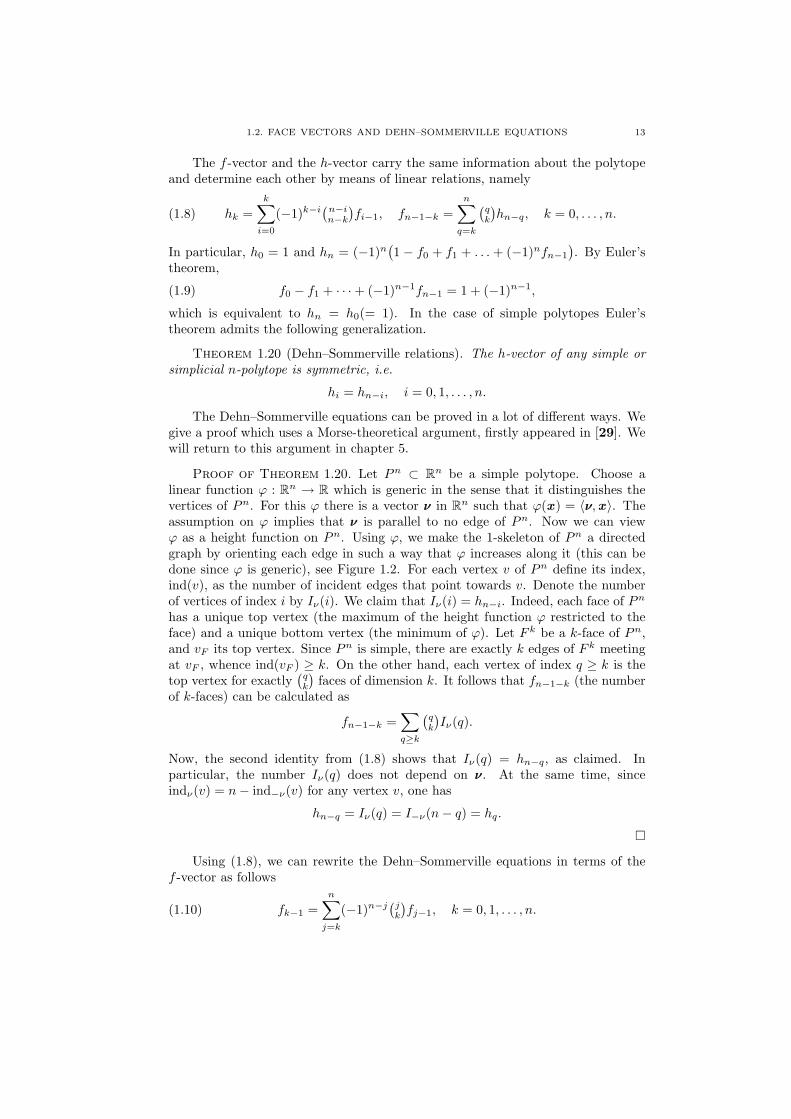
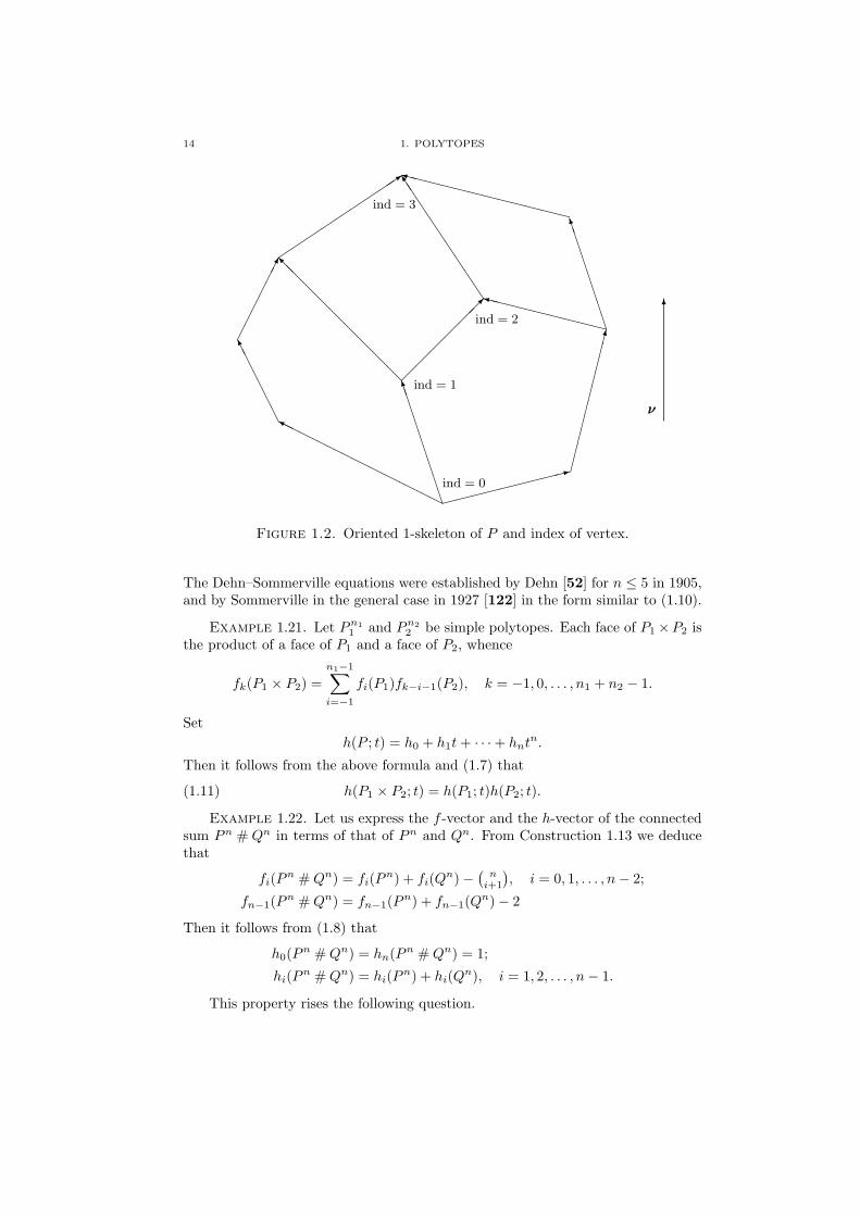
Proof of Theorem 1.20. Let Pn ⊂ Rn be a simple polytope. Choose alinear function ϕ : Rn → R which is generic in the sense that it distinguishes thevertices of Pn. For this ϕ there is a vector νν in Rn such that ϕ(x ) = 〈νν,x 〉. Theassumption on ϕ implies that νν is parallel to no edge of Pn. Now we can viewϕ as a height function on Pn. Using ϕ, we make the 1-skeleton of Pn a directedgraph by orienting each edge in such a way that ϕ increases along it (this can bedone since ϕ is generic), see Figure 1.2. For each vertex v of Pn define its index,ind(v), as the number of incident edges that point towards v. Denote the numberof vertices of index i by Iν(i). We claim that Iν(i) = hn−i. Indeed, each face of Pn
has a unique top vertex (the maximum of the height function ϕ restricted to theface) and a unique bottom vertex (the minimum of ϕ). Let F k be a k-face of Pn,and vF its top vertex. Since Pn is simple, there are exactly k edges of F k meetingat vF , whence ind(vF ) ≥ k. On the other hand, each vertex of index q ≥ k is thetop vertex for exactly
(qk
)faces of dimension k. It follows that fn−1−k (the number
of k-faces) can be calculated as
fn−1−k =∑
q≥k
(qk
)Iν(q).
Now, the second identity from (1.8) shows that Iν(q) = hn−q, as claimed. Inparticular, the number Iν(q) does not depend on νν. At the same time, sinceindν(v) = n− ind−ν(v) for any vertex v, one has
hn−q = Iν(q) = I−ν(n− q) = hq.
¤
Using (1.8), we can rewrite the Dehn–Sommerville equations in terms of thef -vector as follows
(1.10) fk−1 =n∑
j=k
(−1)n−j(
jk
)fj−1, k = 0, 1, . . . , n.
14 1. POLYTOPES
HHHHHHHHHHHHY
BB
BB
BB
BBBM
»»»»»»»»»:¤¤¤¤¤¤¤¤¤¤º
AA
AA
AAK
¡¡
¡¡
¡¡µ
@@
@@
@@
@@@I
¢¢¢¢¢¢
XXXXXXXXXy
BB
BB
BB
BBM
JJ
JJ
JJ
JJJ]
´´
´´
´´
´´3
XXXXXXXXXXXXy
6
νν
ind = 0
ind = 1
ind = 2
ind = 3
Figure 1.2. Oriented 1-skeleton of P and index of vertex.
The Dehn–Sommerville equations were established by Dehn [52] for n ≤ 5 in 1905,and by Sommerville in the general case in 1927 [122] in the form similar to (1.10).
Example 1.21. Let Pn11 and Pn2
2 be simple polytopes. Each face of P1×P2 isthe product of a face of P1 and a face of P2, whence
fk(P1 × P2) =n1−1∑
i=−1
fi(P1)fk−i−1(P2), k = −1, 0, . . . , n1 + n2 − 1.
Seth(P ; t) = h0 + h1t + · · ·+ hntn.
Then it follows from the above formula and (1.7) that
(1.11) h(P1 × P2; t) = h(P1; t)h(P2; t).
Example 1.22. Let us express the f -vector and the h-vector of the connectedsum Pn # Qn in terms of that of Pn and Qn. From Construction 1.13 we deducethat
fi(Pn # Qn) = fi(Pn) + fi(Qn)− (n
i+1
), i = 0, 1, . . . , n− 2;
fn−1(Pn # Qn) = fn−1(Pn) + fn−1(Qn)− 2
Then it follows from (1.8) that
h0(Pn # Qn) = hn(Pn # Qn) = 1;
hi(Pn # Qn) = hi(Pn) + hi(Qn), i = 1, 2, . . . , n− 1.
This property rises the following question.
1.3. THE g-THEOREM 15
Problem 1.23. Describe all integer-valued functions on the set of simple poly-topes which are linear with respect to the connected sum operation.
The previous identities show that examples of such functions are provided byhi for i = 1, . . . , n− 1.
Example 1.24. Suppose S is a q-neighborly simplicial n-polytope (see Defini-tion 1.15) different from the n-simplex. Then fk−1(S) =
(mk
), k ≤ q. From (1.8)
we get
(1.12) hk(S) =k∑
i=0
(−1)k−i(n−ik−i
)(mi
)=
(m−n+k−1
k
), k ≤ q.
The latter equality is obtained by calculating the coefficient of tk from two sides ofthe identity
1(1 + t)n−k+1
(1 + t)m = (1 + t)m−n+k−1.
Since S is not a simplex, we have m > n + 1, which together with (1.12) givesh0 < h1 < · · · < hq. These inequalities together with the Dehn–Sommervilleequations imply the upper bound q ≤ [
n2
]mentioned in Definition 1.15.
1.3. The g-theorem
The g-theorem gives answer to the following natural question: which integervectors may appear as the f -vectors of simple (or, equivalently, simplicial) poly-topes? The Dehn–Sommerville relations provide a necessary condition. As far asonly linear equations are concerned, there are no further restrictions.
Proposition 1.25 (Klee [86]). The Dehn–Sommerville relations are the mostgeneral linear equations satisfied by the f-vectors of all simple (or simplicial) poly-topes.
Proof. In [86] the statement was proved directly, in terms of f -vectors. How-ever, the usage of h-vectors significantly simplifies the proof. It is sufficient to provethat the affine hull of the h-vectors (h0, h1, . . . , hn) of simple n-polytopes is an
[n2
]-
dimensional plane. This can be done, for instance, by providing[n2
]+1 simple poly-
topes with affinely independent h-vectors. Set Qk := ∆k ×∆n−k, k = 0, 1 . . . ,[n2
].
Since h(∆k) = 1 + t + · · ·+ tk, the formula (1.11) gives
h(Qk) =1− tk+1
1− t· 1− tn−k+1
1− t.
It follows that h(Qk+1) − h(Qk) = tk+1 + · · · + tn−k−1, k = 0, 1, . . . ,[n2
] − 1.Therefore, the vectors h(Qk), k = 0, 1 . . . ,
[n2
], are affinely independent. ¤
Example 1.26. Each vertex of a simple n-polytope Pn is contained in exactlyn edges and each edge connects two vertices. This implies the following “obvious”linear equation for the components of the f -vector of Pn:
(1.13) 2fn−2 = nfn−1.
Proposition 1.25 shows that this equation is a corollary of the Dehn–Sommervilleequations. (One may observe that it is equation (1.10) for k = n − 1.) It follows
16 1. POLYTOPES
from (1.13) and Euler identity (1.9) that for simple (or simplicial) 3-polytopes thef -vector is completely determined by the number of facets, namely,
f (P 3) = (f0, 3f0 − 6, 2f0 − 4).
We mention also that Euler identity (1.9) is the only linear relation satisfiedby the face vectors of general convex polytopes. (This can be proved in the similarway as Proposition 1.25, by specifying sufficiently many polytopes with affinelyindependent face vectors.)
The conditions characterizing the f -vectors of simple (or simplicial) polytopes,now know as the g-theorem, were conjectured by P. McMullen [96] in 1970 andproved by R. Stanley [125] (necessity) and Billera, Lee [18] (sufficiency) in 1980.Besides the Dehn–Sommerville equations, the g-theorem contains two groups ofinequalities, one linear and one non-linear. To formulate the g-theorem we needthe following construction.
Definition 1.27. For any two positive integers a, i there exists a unique bi-nomial i-expansion of a of the form
a =(ai
i
)+
(ai−1i−1
)+ · · ·+ (
aj
j
),
where ai > ai−1 > · · · > aj ≥ j ≥ 1. Define
a〈i〉 =(ai+1i+1
)+
(ai−1+1
i
)+ · · ·+ (
aj+1j+1
), 0〈i〉 = 0.
Example 1.28. 1. For a > 0, a〈1〉 =(a+12
).
2. If i ≥ a then the binomial expansion has the form
a =(ii
)+
(i−1i−1
)+ · · ·+ (
i−a+1i−a+1
)= 1 + · · ·+ 1,
and therefore a〈i〉 = a.3. Let a = 28, i = 4. The corresponding binomial expansion is
28 =(64
)+
(53
)+
(32
).
Hence,28〈4〉 =
(75
)+
(64
)+
(43
)= 40.
Theorem 1.29 (g-theorem). An integer vector (f0, f1, . . . , fn−1) is the f -vec-tor of a simple n-polytope if and only if the corresponding sequence (h0, . . . , hn)determined by (1.7) satisfies the following three conditions:
(a) hi = hn−i, i = 0, . . . , n (the Dehn–Sommerville equations);(b) h0 ≤ h1 ≤ · · · ≤ h[
n2
], i = 0, 1, . . . ,[n2
];
(c) h0 = 1, hi+1 − hi ≤ (hi − hi−1)〈i〉, i = 1, . . . ,[n2
]− 1.
Remark. Obviously, the same conditions characterize the f -vectors of simpli-cial polytopes.
Example 1.30. 1. The first inequality h0 ≤ h1 from part (b) of g-theorem isequivalent to f0 = m ≥ n + 1. This just expresses the fact that it takes at leastn + 1 hyperplanes to bound a polytope in Rn.
2. Taking into account that
h2 =(n2
)− (n− 1)f0 + f1
1.3. THE g-THEOREM 17
(see (1.8)), we rewrite the first inequality h2 − h1 ≤ (h1 − h0)〈1〉 from part (c) ofg-theorem as (
n+12
)− nf0 + f1 ≤(f0−n
2
).
(see Example 1.28.1). This is equivalent to the upper bound
f1 ≤(f02
),
which says that two facets share at most one face of codimension two. In the dual”simplicial” notations, two vertices are joined by at most one edge.
3. The second inequality h1 ≤ h2 (for n ≥ 4) from part (b) of g-theorem isequivalent to
f1 ≥ nf0 −(n+1
2
).
This is the first (and most significant) inequality from the famous Lower BoundConjecture for simple polytopes (see Theorem 1.37 below).
-
6
0 h1
h2
¡¡
¡¡
¡¡
¡¡
¡¡
¡¡
¡¡¡h2 = h1(h1+1)
2h2 = h1
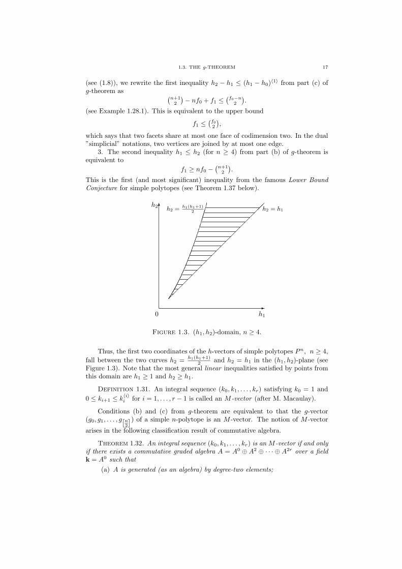
Figure 1.3. (h1, h2)-domain, n ≥ 4.
Thus, the first two coordinates of the h-vectors of simple polytopes Pn, n ≥ 4,fall between the two curves h2 = h1(h1+1)
2 and h2 = h1 in the (h1, h2)-plane (seeFigure 1.3). Note that the most general linear inequalities satisfied by points fromthis domain are h1 ≥ 1 and h2 ≥ h1.
Definition 1.31. An integral sequence (k0, k1, . . . , kr) satisfying k0 = 1 and0 ≤ ki+1 ≤ k
〈i〉i for i = 1, . . . , r − 1 is called an M -vector (after M. Macaulay).
Conditions (b) and (c) from g-theorem are equivalent to that the g-vector(g0, g1, . . . , g[n
2
]) of a simple n-polytope is an M -vector. The notion of M -vector
arises in the following classification result of commutative algebra.
Theorem 1.32. An integral sequence (k0, k1, . . . , kr) is an M -vector if and onlyif there exists a commutative graded algebra A = A0 ⊕ A2 ⊕ · · · ⊕ A2r over a fieldk = A0 such that
(a) A is generated (as an algebra) by degree-two elements;
18 1. POLYTOPES
(b) the dimension of 2i-th graded component of A equals ki:
dimk A2i = ki, i = 1, . . . , r.
This theorem is essentially due to Macaulay, but the above explicit formulation isthat of [124]. The proof can be also found there.
The proof of the sufficiency part of g-theorem, due to Billera and Lee, is quiteelementary and relies upon a remarkable combinatorial-geometrical construction ofa simplicial polytope with any prescribed M -sequence as its g-vector. On the otherhand, Stanley’s proof of the necessity part of g-theorem (i.e. that the g-vectorof a simple polytope is an M -vector) used deep results from algebraic geometry,in particular, the Hard Lefschetz theorem for the cohomology of toric varieties.We outline Stanley’s proof in section 5.1. After 1993 several more elementarycombinatorial proofs of the g-theorem appeared. The first such proof is due toMcMullen [97]. It builds up on the notion of polytope algebra, which substitutes thecohomology algebra of toric variety. Despite being elementary, it was a complicatedproof. Later, McMullen simplified his approach in [98]. Yet another elementaryproof of the g-theorem has been recently found by Timorin [133]. It relies onthe interpretation of McMullen’s polytope algebra as the algebra of differentialoperators (with constant coefficients) vanishing on the volume polynomial of thepolytope.
1.4. Upper Bound and Lower Bound theorems
The following statement, now know as the Upper Bound Conjecture (UBC),was suggested by Motzkin in 1957 and proved by P. McMullen [95] in 1970.
Theorem 1.33 (UBC for simplicial polytopes). From all simplicial n-polyto-pes S with m vertices the cyclic polytope Cn(m) (Example 1.17) has the maximalnumber of i-faces, 2 ≤ i ≤ n− 1. That is, if f0(S) = m, then
fi(S) ≤ fi
(Cn(m)
)for i = 2, . . . , n− 1.
The equality in the above formula holds if and only if S is a neighborly polytope (seeDefinition 1.15).
Note that since Cn(m) is neighborly,
fi
(Cn(m)
)=
(m
i+1
)for i = 0, . . . ,
[n2
]− 1.
Due to the Dehn–Sommerville equations this determines the full f -vector of Cn(m).The exact values are given by the following lemma.
Lemma 1.34. The number of i-faces of cyclic polytope Cn(m) (or any neighborlyn-polytope with m vertices) is given by
fi
(Cn(m)
)=
[n2
]∑q=0
(q
n−1−i
)(m−n+q−1
q
)+
[n−1
2
]∑p=0
(n−p
i+1−p
)(m−n+p−1
p
), i = −1, . . . , n−1,
where we assume(pq
)= 0 for p < q.
1.4. UPPER BOUND AND LOWER BOUND THEOREMS 19
Proof. Using the second identity from (1.8), identity[n2
]+1 = n− [
n−12
], the
Dehn–Sommerville equations, and (1.12), we calculate
fi =n∑
q=0
(q
n−1−i
)hn−q =
[n2
]∑q=0
(q
n−1−i
)hq +
n∑
q=[n2
]+1
(q
n−1−i
)hn−q
=
[n2
]∑q=0
(q
n−1−i
)(m−n+q−1
q
)+
[n−1
2
]∑p=0
(n−p
i+1−p
)(m−n+p−1
p
).
¤
The above proof justifies the following statement.
Corollary 1.35. The UBC for simplicial polytopes (Theorem 1.33) is impliedby the following inequalities for the h-vector of a simplicial polytope S with mvertices
hi(S) ≤ (m−n+i−1
i
), i = 0, . . . ,
[n2
].
This was one of the key observations in McMullen’s original proof of the UBCfor simplicial polytopes (see also [29, §18] and [145, §8.4]). The above corollaryis also useful for different generalization of UBC (we will return to this in sec-tion 3.2). We note also that due to the argument of Klee and McMullen (see [145,Lemma 8.24]) the UBT holds for all convex polytopes, not necessarily simplicial.That is, the cyclic polytope Cn(m) has the maximal number of i-faces from allconvex n-polytopes with m vertices.
Another fundamental fact from the theory of convex polytopes is the LowerBound Conjecture (LBC) for simplicial polytopes.
Definition 1.36. A simplicial n-polytope S is called stacked if there is a se-quence S0, S1, . . . , Sk = S of n-polytopes such that S0 is an n-simplex and Si+1 isobtained from Si by adding a pyramid over some facet of Si. In the combinatoriallanguage, stacked polytopes are those obtained from a simplex by applying severalsubsequent stellar subdivisions of facets.
Remark. Adding a pyramid (or stellar subdivision of a facet) is dual to “cut-ting a vertex” of a simple polytope (see Example 1.14.3).
Theorem 1.37 (LBC for simplicial polytopes). For any simplicial n-polytopeS (n ≥ 3) with m = f0 vertices hold
fi(S) ≥ (ni
)f0 −
(n+1i+1
)i for i = 1, . . . , n− 2;
fn−1(S) ≥ (n− 1)f0 − (n + 1)(n− 2).
The equality is achieved if and only if S is a stacked polytope.
The argument by McMullen, Perles and Walkup [100] reduces the LBC to thecase i = 1, namely, the inequality f1 ≥ f0 −
(n+1
2
). The LBC was first proved by
Barnette [13], [15]. The “only if” part in the statement about the equality wasproved in [19] using g-theorem. Unlike the UBC, little is know about generaliza-tions of the LBC theorem to non-simplicial convex polytopes. Some results in thisdirection were obtained in [83] along with generalizations of the LBC theorem tosimplicial spheres and manifolds (see also sections 2.3–2.4 in this book).
20 1. POLYTOPES
In dual notations, the UBC and the LBC provide upper and lower bounds forthe number of faces of simple polytopes with given number of facets. Both theoremswere proved approximately at the same time (in 1970) and motivated P. McMullento conjecture the g-theorem [96]. On the other hand, both UBC and LBC arecorollaries of the g-theorem (see e.g. [29, §20]). In fact the LBC follows only fromparts (a) and (b) of Theorem 1.29, while the UBC follows from parts (a) and (c).
Part (b) of g-theorem, namely the inequalities
(1.14) h0 ≤ h1 ≤ · · · ≤ h[n2
],
where suggested in [100] as a generalization of the LBC for simplicial polytopes.The second inequality h1 ≤ h2 is equivalent to the i = 1 case of LBC (see Exam-ple 1.30.3). It follows from the results of [100] and [19] that (1.14) are the strongestpossible linear inequalities satisfied by the f -vectors of simple (or simplicial) poly-topes (compare with the comment after Example 1.30). These inequalities are nowknown as the Generalized Lower Bound Conjecture (GLBC).
During the last two decades a lot of work was done in extending the Dehn–Sommerville equations, the GLBC and the g-theorem to objects more general thansimplicial polytopes. However, there is still a lot of intriguing open problems here.For more information see the first section of survey article [129] by Stanley andsection 2.3 in this book.
1.5. Stanley–Reisner face rings of simple polytopes
The only aim of this short section is to define the Stanley–Reisner ring ofa simple polytope. This fundamental combinatorial invariant will be one of themain characters in the next chapter. However, it is convenient for us to give it anindependent treatment in the polytopal case.
Let P be a simple n-polytope with m facets F1, . . . , Fm. Fix a commutative ringk with unit. Let k[v1, . . . , vm] be the polynomial algebra over k on m generators.We make it a graded algebra by setting deg(vi) = 2.
Definition 1.38. The face ring (or the Stanley–Reisner ring) of a simplepolytope P is the quotient ring
k(P ) = k[v1, . . . , vm]/IP ,
where IP is the ideal generated by all square-free monomials vi1vi2 · · · vis such thatFi1 ∩ · · · ∩ Fis = ∅ in P , i1 < · · · < is.
Since IP is a homogeneous ideal, k(P ) is a graded k-algebra.
Remark. In certain circumstances it is convenient to choose a different grad-ing in k[v1, . . . , vm] and correspondingly k(K). These cases will be particularlymentioned.
Example 1.39. 1. Let Pn be the n-simplex (regarded as a simple polytope).Then
k(Pn) = k[v1, . . . , vn+1]/(v1v2 · · · vn+1).2. Let P be the 3-cube I3. Then
k(P ) = k[v1, v2 . . . , v6]/(v1v4, v2v5, v3v6).
3. Let P 2 be the m-gon, m ≥ 4. Then
IP 2 = (vivj : i− j 6= 0,±1 mod m).
CHAPTER 2
Topology and combinatorics of simplicialcomplexes
Simplicial complexes or triangulations (first introduced by Poincare) providean elegant, rigorous and convenient tool for studying topological invariants by com-binatorial methods. The algebraic topology itself evolved from studying triangu-lations of topological spaces. With the appearance of cellular (or CW) complexesalgebraic tools gradually replaced the combinatorial ones in topology. However,simplicial complexes have always played a significant role in PL topology, discreteand combinatorial geometry. The convex geometry provides an important class ofsphere triangulations which are the boundary complexes of simplicial polytopes.The emergence of computers resulted in regaining the interest to “CombinatorialTopology”, since simplicial complexes provide the most effective way to translatetopological structures into machine language. So, it seems to be the proper timefor topologists to get use of remarkable achievements in discrete and combinatorialgeometry of the last decades, which we started to review in the previous chapter.
2.1. Abstract simplicial complexes and polyhedrons
Let S be a finite set. Given a subset σ ⊂ S, we denote its cardinality by |σ|.Definition 2.1. An (abstract) simplicial complex on the set S is a collection
K = σ of subsets of S such that for each σ ∈ K all subsets of σ (including ∅) alsobelong to K. A subset σ ∈ K is called an (abstract) simplex of K. One-elementsubsets are called vertices of K. If K contains all one-element subsets of S, thenwe say that K is a simplicial complex on the vertex set S. The dimension of anabstract simplex σ ∈ K is its cardinality minus one: dim σ = |σ|−1. The dimensionof an abstract simplicial complex is the maximal dimension of its simplices. Asimplicial complex K is pure if all its maximal simplices have the same dimension.A subcollection K ′ ⊂ K which is also a simplicial complex is called a subcomplexof K.
In most of our constructions it is safe to fix an ordering in S and identify Swith the index set [m] = 1, . . . , m. This makes notations more clear; however, insome cases it is more convenient to keep unordered sets.
To distinguish from abstract simplices, the convex polytopes introduced inExample 1.7 (i.e. the convex hulls of affinely independent points) will be referredto as geometrical simplices.
Definition 2.2. A geometrical simplicial complex (or a polyhedron) is a subsetP ⊂ Rn represented as a finite union U of geometrical simplices of any dimensionsin such a way that the following two conditions are satisfied:
(a) each face of a simplex in U belongs to U ;
21
22 2. TOPOLOGY AND COMBINATORICS OF SIMPLICIAL COMPLEXES
(b) the intersection of any two simplices in U is a face of each.A geometrical simplex from U is called a face of P; as usual, one-dimensional facesare vertices. The dimension of P is the maximal dimension of its faces.
Agreement. The notion of polyhedron from Definition 1.2 is not the sameas that from Definition 2.2. The first meaning of the term “polyhedron” (i.e. the“unbounded polytope”) is adopted in the convex geometry, while the second one(i.e. the “geometrical simplicial complex”) is used in the combinatorial topology.Since both terms have become standard in the appropriate science, we can notchange their names completely. We will use “polyhedron” for a geometrical simpli-cial complex and “convex polyhedron” for an “unbounded polytope”. Anyway, itwill be always clear from the context which “polyhedron” is under consideration.
In the sequel both abstract and geometrical simplicial complexes are assumedto be finite.
Agreement. Depending on the context, we will denote by ∆m−1 three differ-ent objects: the abstract simplicial complex 2[m] consisting of all subsets of [m],the convex polytope from Example 1.7 (i.e. the geometrical simplex), and thegeometrical simplicial complex which is the union of all faces of the geometricalsimplex.
Definition 2.3. Given a simplicial complex K on the vertex set [m], say thata polyhedron P is a geometrical realization of K if there is a bijection between theset [m] and the vertex set of P that takes simplices of K to vertex sets of facesof P.
If we do not care about the dimension of the ambient space, then there is thefollowing quite obvious way to construct a geometrical realization for any simplicialcomplex K.
Construction 2.4. Suppose K is a simplicial complex on the set [m]. Let e i
denote the i-th unit coordinate vector in Rm. For each subset σ ⊂ [m] denote by∆σ the convex hull of vectors e i with i ∈ σ. Then ∆σ is a (regular, geometrical)simplex. The polyhedron ⋃
σ∈K
∆σ ⊂ Rm
is a geometrical realization of K.
The above construction is just a geometrical interpretation of the fact that anysimplicial complex on [m] is a subcomplex of the simplex ∆m−1. At the same timeit is a classical result [115] that any n-dimensional abstract simplicial complex Kn
admits a geometrical realization in (2n + 1)-dimensional space.
Example 2.5. Let S be a simplicial n-polytope. Then its boundary ∂S is a(geometrical) simplicial complex homeomorphic to an (n−1)-sphere. This examplewill be important in section 2.3.
Definition 2.6. The f -vector, the h-vector and the g-vector of an (n − 1)-dimensional simplicial complex Kn−1 are defined in the same way as for simpli-cial polytopes. Namely, f (Kn−1) = (f0, f1, . . . , fn−1), where fi is the number ofi-dimensional simplices of Kn−1, and h(Kn−1) = (h0, h1, . . . , hn), where hi aredetermined by (1.7). Here we also assume f−1 = 1. If Kn−1 = ∂S, the boundaryof a simplicial n-polytope S, then one obviously has f (Kn−1) = f (S).
2.2. BASIC PL TOPOLOGY, AND OPERATIONS WITH SIMPLICIAL COMPLEXES 23
2.2. Basic PL topology, and operations with simplicial complexes
For a detailed exposition of PL (piecewise linear) topology we refer to theclassical monographs [77] by Hudson and [118] by Rourke and Sanderson. Therole of PL category in the modern topology is described, for instance, in the morerecent book [104] by Novikov.
Definition 2.7. Let K1, K2 be simplicial complexes on the sets [m1], [m2]respectively, and P1, P2 their geometrical realizations. A map φ : [m1] → [m2] issaid to be a simplicial map between K1 and K2 if φ(σ) ∈ K2 for any σ ∈ K1. Asimplicial map φ is said to be non-degenerate if |φ(σ)| = |σ| for any σ ∈ K1. Onthe geometrical level, a simplicial map extends linearly on the faces of P1 to a mapφ : P1 → P2 (denoted by the same letter for simplicity). We refer to the lattermap as a simplicial map of polyhedrons. A simplicial isomorphism of polyhedronsis a simplicial map for which there exists a simplicial inverse. A polyhedron P ′ iscalled a subdivision of polyhedron P if each simplex of P ′ is contained in a simplexof P and each simplex of P is a union of finitely many simplices of P ′. A PL mapφ : P1 → P2 is a map that is simplicial between some subdivisions of P1 and P2.A PL homeomorphism is a PL map for which there exists a PL inverse. Two PLhomeomorphic polyhedrons sometimes are also called combinatorially equivalent .In other words, two polyhedrons P1,P2 are PL homeomorphic if and only if thereexists a polyhedron P isomorphic to a subdivision of each of them.
Example 2.8. For any simplicial complex K on [m] there exists a simplicialmap (inclusion) K → ∆m−1.
There is an obvious simplicial homeomorphism between any two geometricalrealizations of a given simplicial complex K. This justifies our single notation |K|for any geometrical realization of K. Whenever it is safe, we do not distinguishbetween abstract simplicial complexes and their geometrical realizations. For ex-ample, we would say “simplicial complex K is PL homeomorphic to X” instead of“the geometrical realisation of K is PL homeomorphic to X”.
Construction 2.9 (join of simplicial complexes). Let K1, K2 be simplicialcomplexes on sets S1 and S2 respectively. The join of K1 and K2 is the simplicialcomplex
K1 ∗K2 :=σ ⊂ S1 ∪ S2 : σ = σ1 ∪ σ2, σ1 ∈ K1, σ2 ∈ K2
on the set S1 ∪ S2. If K1 is realized in Rn1 and K2 in Rn2 , then there is obviouscanonical geometrical realisation of K1 ∗K2 in Rn1+n2 = Rn1 × Rn2 .
Example 2.10. 1. If K1 = ∆m1−1, K2 = ∆m2−1, then K1 ∗K2 = ∆m1+m2−1.2. The simplicial complex ∆0 ∗K (the join of K and a point) is called the cone
over K and denoted cone(K).3. Let S0 be a pair of disjoint points (a 0-sphere). Then S0 ∗K is called the
suspension of K and denoted ΣK. The geometric realization of cone(K) (of ΣK)is the topological cone (suspension) over |K|.
4. Let P1 and P2 be simple polytopes. Then
∂((P1 × P2)∗
)= ∂(P ∗1 P ∗2 ) = (∂P ∗1 ) ∗ (∂P ∗2 ).
(see Construction 1.12).
24 2. TOPOLOGY AND COMBINATORICS OF SIMPLICIAL COMPLEXES
Construction 2.11. The fact that the product of two simplices is not a sim-plex causes some problems with triangulating the products of spaces. However,there is a canonical triangulation of the product of two polyhedra for each choiceof orderings of their vertices. So suppose K1, K2 are simplicial complexes on [m1]and [m2] respectively (this is one of the few constructions where the ordering ofvertices is significant). Then we construct a new simplicial complex on [m1]× [m2],which we call the Cartesian product of K1 and K2 and denote K1×K2, as follows.By definition, a simplex of K1 × K2 is a subset of some σ1 × σ2 (with σ1 ∈ K1,σ2 ∈ K2) that establishes a non-decreasing correspondence between σ1 and σ2.More formally,
K1 ×K2 :=σ ⊂ σ1 × σ2 : σ1 ∈ K1, σ2 ∈ K2,
and i ≤ i′ implies j ≤ j′ for any two pairs (i, j), (i′, j′) ∈ σ.
The polyhedron |K1 ×K2| defines a canonical triangulation of |K1| × |K2|.Construction 2.12 (connected sum of simplicial complexes). Let K1, K2
be two pure (n − 1)-dimensional simplicial complexes on sets S1, S2 respectively,|S1| = m1, |S2| = m2. Suppose we are given two maximal simplices σ1 ∈ K1,σ2 ∈ K2. Fix an identification of σ1 and σ2, and denote by S1 ∪σ S2 the unionof S1 and S2 with σ1 and σ2 identified (the subset created by the identification isdenoted σ). We have |S1 ∪σ S2| = m1 + m2 − n. Both K1 and K2 now can beviewed as collections of subsets of S1 ∪σ S2. We define the connected sum of K1 atσ1 and K2 at σ2 to be the simplicial complex
K1 #σ1,σ2 K2 := (K1 ∪K2) \ σon the set S1 ∪σ S2. When the choices of σ1, σ2 and identification of σ1 and σ2 areclear we use the abbreviation K1 # K2. Geometrically, the connected sum of |K1|and |K2| at σ1 and σ2 is produced by attaching |K1| to |K2| along the faces σ1, σ2
and then removing the face σ obtained from the identification of σ1 with σ2.
Example 2.13. 1. Let K1 be an (n − 1)-simplex, and K2 a pure (n − 1)-dimensional complex with a fixed maximal simplex σ2. Then K1 #K2 = K2 \σ2,i.e. K1 # K2 is obtained by deleting the simplex σ2 from K2.
2. Let P1 and P2 be simple polytopes. Set K1 = ∂(P ∗1 ), K2 = ∂(P ∗2 ). Then
K1 # K2 = ∂((P1 # P2)∗
)
(see Construction 1.13).
Definition 2.14. The barycentric subdivision of an abstract simplicial complexK is the simplicial complex K ′ on the set σ ∈ K of simplices of K whose simplicesare chains of embedded simplices of K. That is, σ1, . . . , σr ∈ K ′ if and only ifσ1 ⊂ σ2 ⊂ · · · ⊂ σr in K (after possible re-ordering).
The barycenter of a (polytopal) simplex ∆n ⊂ Rn with vertices v1, . . . , vn+1
is the point bc(∆n) = 1n+1 (v1 + · · · + vn+1) ∈ ∆n. The barycentric subdivision
P ′ of a polyhedron P is defined as follows. The vertex set of P ′ is formed by thebarycenters of simplices of P. A collection of barycenters bc(∆i1
1 ), . . . , bc(∆irr )
spans a simplex of P ′ if and only if ∆i11 ⊂ · · · ⊂ ∆ir
r in P. Obviously |K ′| = |K|′for any abstract simplicial complex K.
Example 2.15. For any (n − 1)-dimensional simplicial complex Kn−1 on [m]there is a non-degenerate simplicial map K ′ → ∆n−1 defined on the vertices by
2.2. BASIC PL TOPOLOGY, AND OPERATIONS WITH SIMPLICIAL COMPLEXES 25
σ → |σ|, σ ∈ K. (Here σ is regarded as a vertex of K ′ and |σ| as a vertex of∆n−1.)
Example 2.16. Let K be a simplicial complex on a set S, and suppose we aregiven a choice function f : K → S assigning to each simplex σ ∈ K a point in σ. Forinstance, if S = [m] we can take f = min, that is, assign to each simplex its minimalvertex. For every such map f there is a canonical simplicial map ∇f : K ′ → Kconstructed as follows. By the definition of K ′, the vertices of K ′ are in one-to-onecorrespondence with the simplices of K. For each σ ∈ K (regarded as a vertex ofK ′) set ∇f (σ) = f(σ). This extends to the simplices of K ′ by
∇f (σ1 ⊂ σ2 ⊂ · · · ⊂ σr) = f(σ1), f(σ2), . . . , f(σr).The latter is a subset of σr, whence it is a simplex of K. Thus, ∇f is indeed asimplicial map.
Example 2.17 (order complex of a poset). Let S be any poset. Define ord(S)to be the collection of all chains x1 < x2 < · · · < xk, xi ∈ S. Then ord(S) is clearlya simplicial complex. It is called the order complex of the poset (S, <). The ordercomplex of the inclusion poset of non-empty simplices of a simplicial complex K isits barycentric subdivision K ′. If we add the empty simplex to the poset, then theresulting order complex will be coneK ′.
Definition 2.18. A simplicial complex K is called a flag complex if any set ofvertices which are pairwise connected spans a simplex of K.
Proposition 2.19. For each simplicial graph (1-dimensional simplicial com-plex) Γ there exists a unique flag complex KΓ on the same vertex set whose 1-skeleton is Γ.
Proof. The simplices of KΓ are the vertex sets of complete subgraphs in Γ. ¤
Definition 2.20. The minimal simplicial complex that contains a given com-plex K and is flag is called the flagification of K and denoted fla(K).
Definition 2.21. Given a simplicial complex K on S, a missing face of K isa subset σ ⊂ [m] such that σ /∈ K, but every proper subset of σ is a simplex of K.
The following statement is straightforward.
Proposition 2.22. K is a flag complex if and only if every its missing facehas two vertices.
Example 2.23. 1. Order complexes of posets (in particular, barycentric sub-divisions) are examples of flag complexes. On the other hand, the boundary of a5-gon is flag complex, but not an order complex of poset.
2. Let K = K1 #σ1,σ2 K2 (see Construction 2.12). Then σ is a missing face ofK provided that at least one of K1 and K2 is not a simplex.
Definition 2.24. The link and the star of a simplex σ ∈ K are the subcom-plexes
linkK σ =τ ∈ K : σ ∪ τ ∈ K, σ ∩ τ = ∅
;
starK σ =τ ∈ K : σ ∪ τ ∈ K
.
26 2. TOPOLOGY AND COMBINATORICS OF SIMPLICIAL COMPLEXES
For any vertex v ∈ K the subcomplex starK v can be identified with the cone overlinkK v. The polyhedron | starK v| consists of all faces of |K| that contain v. Weomit the subscripts K whenever the context allows.
For any subcomplex L ⊂ K define the (closed) combinatorial neighborhoodUK(L) of L in K by
UK(L) =⋃
σ∈L
starK σ.
Equivalently, the combinatorial neighborhood UK(L) consists of all simplices ofK, together with all their faces, having some simplex of L as a face. Define alsothe open combinatorial neighborhood
U K(L) of |L| in |K| as the union of relative
interiors of faces of |K| having some simplex of |L| as their face.For any subset σ ⊂ S define the full subcomplex Kσ by
(2.1) Kσ =τ ∈ K : τ ⊂ σ
.
Set coreS = v ∈ S : star v 6= K. The core of K is the subcomplex core K =KcoreS . Thus, the core is the maximal subcomplex containing all vertices whosestars do not coincide with K.
Example 2.25. 1. linkK ∅ = K.2. Let K = ∂∆3 be the boundary of the tetrahedron on four vertices 1, 2, 3, 4,
and σ = 1, 2. Then link σ is the subcomplex consisting of two disjoint points 3and 4.
3. Let K be the cone over L with vertex v. Then link v = L, star v = K, andcoreK ⊂ L.
Example 2.26 (dual simplicial complex). Let K be a simplicial complex on S.Suppose that K is not the full simplex on S. Define
K :=σ ⊂ S : S \ σ /∈ K
.
Then K is also a simplicial complex on S. It is called the dual of K.
The dual simplicial complex K provides the following “purely simplicial in-terpretation” for the Alexander duality (see e.g. [104, p. 54]) between |K| andSm−1 \ |K| for any simplicial complex K embedded in the (m − 1)-sphere. Letus consider the barycentric subdivision (∂∆m−1)′ of the boundary of a geometricalsimplex on the vertex set [m] = 1, . . . , m. By the definition, the faces of (∂∆m−1)′
correspond to the pairs σ ⊂ τ of subsets of [m] satisfying |σ| ≥ 1, |τ | ≤ m − 1.Denote the corresponding faces by ∆σ⊂τ . (For example, ∆i⊂i is the vertexv = i of ∆m−1 regarded as a vertex of (∂∆m−1)′.) Denote i = [m] \ i and,more generally, σ = [m] \ σ for any subset σ ⊂ [m]. For any simplicial complex Kon [m] define the following subcomplex in (∂∆m−1)′:
D(K) =⋃
σ,τ :τ⊂σ,σ/∈K
∆bσ⊂bτ .
Proposition 2.27. For any simplicial complex K 6= ∆m−1 on the set [m] thepolyhedron D(K) provides a geometrical realisation for the barycentric subdivisionof the dual simplicial complex:
D(K) = |K ′|.
2.2. BASIC PL TOPOLOGY, AND OPERATIONS WITH SIMPLICIAL COMPLEXES 27
Moreover, if the barycentric subdivision of K is realized canonically as a subpoly-hedron in (∂∆m−1)′, then
|K ′| = (∂∆m−1
)′ \ U (∂∆m−1)′
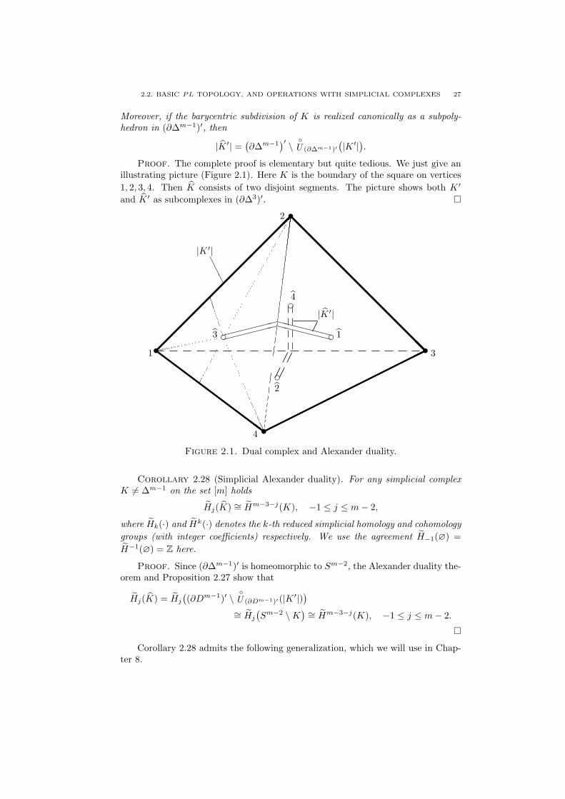
(|K ′|).Proof. The complete proof is elementary but quite tedious. We just give an
illustrating picture (Figure 2.1). Here K is the boundary of the square on vertices1, 2, 3, 4. Then K consists of two disjoint segments. The picture shows both K ′
and K ′ as subcomplexes in (∂∆3)′. ¤
t1
t2
t3
t4
ZZ
ZZ
ZZ
ZZ
ZZ
ZZ
ZZ
ZZ
ZZ
ZZ
ZZ
ZZ
ZZ
ZZ
ZZ
ZZ
ZZ
ZZ
ZZ
ZZ
ZZ
ZZ
ZZ
ZZ
ZZ
ZZ
ZZ
ZZ
ZZ
ZZ
ZZ
ZZ
ZZ
ZZ
ZZ
ZZ
ZZ
ZZ
ZZ
ZZ
ZZ
ZZ
ZZ
ZZ
ZZ
ZZ
ZZ
ZZ
ZZ
ZZ
ZZ
ZZ
ZZ
ZZ
¡¡
¡¡
¡¡
¡¡
¡¡
¡¡
¡¡¡
¡¡
¡¡
¡¡
¡¡
¡¡
¡¡
¡¡¡
¡¡
¡¡
¡¡
¡¡
¡¡
¡¡
¡¡¡
¡¡
¡¡
¡¡
¡¡
¡¡
¡¡
¡¡¡
¡¡
¡¡
¡¡
¡¡
¡¡
¡¡
¡¡¡
¡¡
¡¡
¡¡
¡¡
¡¡
¡¡
¡¡¡
¡¡
¡¡
¡¡
¡¡
¡¡
¡¡
¡¡¡
¡¡
¡¡
¡¡
¡¡
¡¡
¡¡
¡¡¡
¡¡
¡¡
¡¡
¡¡
¡¡
¡¡
¡¡¡@
@@
@@
@@
@@
@@
@@
@@
@@
@@
@@
@@
@@
@@
@@@
@@
@@
@@
@@
@@
@@
@@@
@@
@@
@@
@@
@@
@@
@@@
@@
@@
@@
@@
@@
@@
@@@
@@
@@
@@
@@
@@
@@
@@@
@@
@@
@@
@@
@@
@@
@@@
@@
@@
@@
@@
@@
@@
@@@
@@
@@
@@
@@
@@
@@
@@@
©©©©©©©©©©©©©©©©©©
©©©©©©©©©©©©©©©©©©
©©©©©©©©©©©©©©©©©©
©©©©©©©©©©©©©©©©©©
©©©©©©©©©©©©©©©©©©
©©©©©©©©©©©©©©©©©©
©©©©©©©©©©©©©©©©©©
©©©©©©©©©©©©©©©©©©
©©©©©©©©©©©©©©©©©©
©©©©©©©©©©©©©©©©©©
©©©©©©©©©©©©©©©©©©
d3 d1»»»»»»»»»»»»
XXXXXXXXXXXX
d2
d4
¢¢
¢¢
¢¢
¢¢
|K ′|¢¢
AAA
|K ′|
Figure 2.1. Dual complex and Alexander duality.
Corollary 2.28 (Simplicial Alexander duality). For any simplicial complexK 6= ∆m−1 on the set [m] holds
Hj(K) ∼= Hm−3−j(K), −1 ≤ j ≤ m− 2,
where Hk(·) and Hk(·) denotes the k-th reduced simplicial homology and cohomologygroups (with integer coefficients) respectively. We use the agreement H−1(∅) =H−1(∅) = Z here.
Proof. Since (∂∆m−1)′ is homeomorphic to Sm−2, the Alexander duality the-orem and Proposition 2.27 show that
Hj(K) = Hj
((∂Dm−1)′ \
U (∂Dm−1)′(|K ′|))
∼= Hj
(Sm−2 \K
) ∼= Hm−3−j(K), −1 ≤ j ≤ m− 2.
¤Corollary 2.28 admits the following generalization, which we will use in Chap-
ter 8.
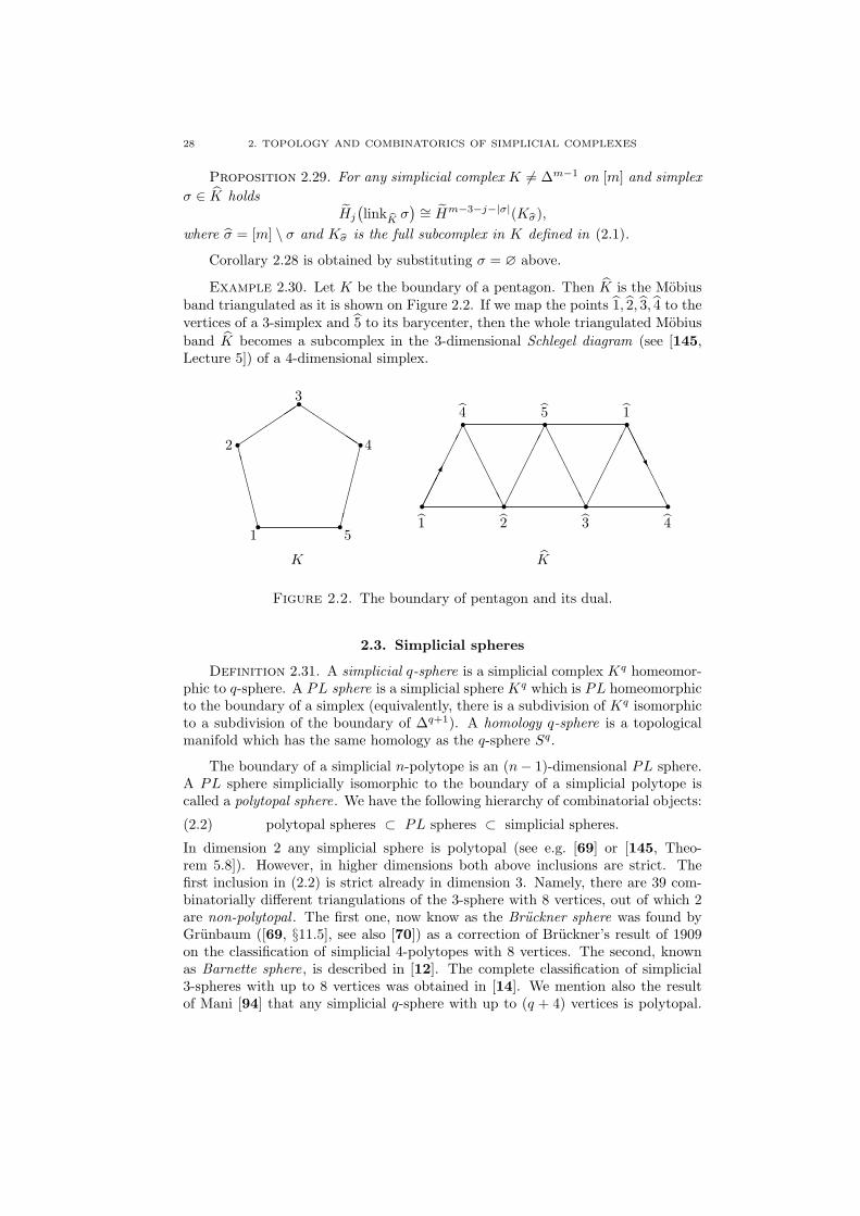
28 2. TOPOLOGY AND COMBINATORICS OF SIMPLICIAL COMPLEXES
Proposition 2.29. For any simplicial complex K 6= ∆m−1 on [m] and simplexσ ∈ K holds
Hj
(link bK σ
) ∼= Hm−3−j−|σ|(Kbσ),where σ = [m] \ σ and Kbσ is the full subcomplex in K defined in (2.1).
Corollary 2.28 is obtained by substituting σ = ∅ above.
Example 2.30. Let K be the boundary of a pentagon. Then K is the Mobiusband triangulated as it is shown on Figure 2.2. If we map the points 1, 2, 3, 4 to thevertices of a 3-simplex and 5 to its barycenter, then the whole triangulated Mobiusband K becomes a subcomplex in the 3-dimensional Schlegel diagram (see [145,Lecture 5]) of a 4-dimensional simplex.
r
r
r
r
rr r r r
r r r
CCCCCC´
´´
QQQ
¤¤¤¤¤¤
¢¢¢¢¢¢
¢¢¢¢¢¢
¢¢¢¢¢¢
¢¢¢
AAAAAA
AAAAAA
AAAAAA
AAAU
1
2
3
4
51 2 3 4
4 5 1
K K
Figure 2.2. The boundary of pentagon and its dual.
2.3. Simplicial spheres
Definition 2.31. A simplicial q-sphere is a simplicial complex Kq homeomor-phic to q-sphere. A PL sphere is a simplicial sphere Kq which is PL homeomorphicto the boundary of a simplex (equivalently, there is a subdivision of Kq isomorphicto a subdivision of the boundary of ∆q+1). A homology q-sphere is a topologicalmanifold which has the same homology as the q-sphere Sq.
The boundary of a simplicial n-polytope is an (n− 1)-dimensional PL sphere.A PL sphere simplicially isomorphic to the boundary of a simplicial polytope iscalled a polytopal sphere. We have the following hierarchy of combinatorial objects:
(2.2) polytopal spheres ⊂ PL spheres ⊂ simplicial spheres.
In dimension 2 any simplicial sphere is polytopal (see e.g. [69] or [145, Theo-rem 5.8]). However, in higher dimensions both above inclusions are strict. Thefirst inclusion in (2.2) is strict already in dimension 3. Namely, there are 39 com-binatorially different triangulations of the 3-sphere with 8 vertices, out of which 2are non-polytopal . The first one, now know as the Bruckner sphere was found byGrunbaum ([69, §11.5], see also [70]) as a correction of Bruckner’s result of 1909on the classification of simplicial 4-polytopes with 8 vertices. The second, knownas Barnette sphere, is described in [12]. The complete classification of simplicial3-spheres with up to 8 vertices was obtained in [14]. We mention also the resultof Mani [94] that any simplicial q-sphere with up to (q + 4) vertices is polytopal.
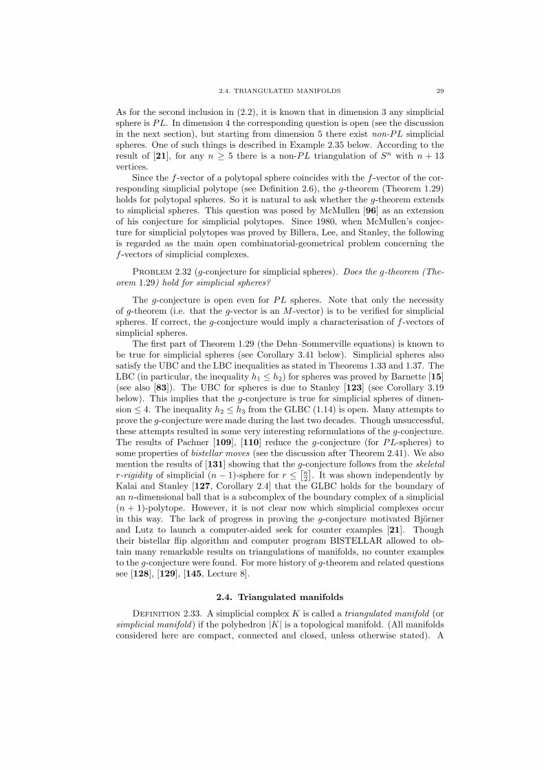
2.4. TRIANGULATED MANIFOLDS 29
As for the second inclusion in (2.2), it is known that in dimension 3 any simplicialsphere is PL. In dimension 4 the corresponding question is open (see the discussionin the next section), but starting from dimension 5 there exist non-PL simplicialspheres. One of such things is described in Example 2.35 below. According to theresult of [21], for any n ≥ 5 there is a non-PL triangulation of Sn with n + 13vertices.
Since the f -vector of a polytopal sphere coincides with the f -vector of the cor-responding simplicial polytope (see Definition 2.6), the g-theorem (Theorem 1.29)holds for polytopal spheres. So it is natural to ask whether the g-theorem extendsto simplicial spheres. This question was posed by McMullen [96] as an extensionof his conjecture for simplicial polytopes. Since 1980, when McMullen’s conjec-ture for simplicial polytopes was proved by Billera, Lee, and Stanley, the followingis regarded as the main open combinatorial-geometrical problem concerning thef -vectors of simplicial complexes.
Problem 2.32 (g-conjecture for simplicial spheres). Does the g-theorem (The-orem 1.29) hold for simplicial spheres?
The g-conjecture is open even for PL spheres. Note that only the necessityof g-theorem (i.e. that the g-vector is an M -vector) is to be verified for simplicialspheres. If correct, the g-conjecture would imply a characterisation of f -vectors ofsimplicial spheres.
The first part of Theorem 1.29 (the Dehn–Sommerville equations) is known tobe true for simplicial spheres (see Corollary 3.41 below). Simplicial spheres alsosatisfy the UBC and the LBC inequalities as stated in Theorems 1.33 and 1.37. TheLBC (in particular, the inequality h1 ≤ h2) for spheres was proved by Barnette [15](see also [83]). The UBC for spheres is due to Stanley [123] (see Corollary 3.19below). This implies that the g-conjecture is true for simplicial spheres of dimen-sion ≤ 4. The inequality h2 ≤ h3 from the GLBC (1.14) is open. Many attempts toprove the g-conjecture were made during the last two decades. Though unsuccessful,these attempts resulted in some very interesting reformulations of the g-conjecture.The results of Pachner [109], [110] reduce the g-conjecture (for PL-spheres) tosome properties of bistellar moves (see the discussion after Theorem 2.41). We alsomention the results of [131] showing that the g-conjecture follows from the skeletalr-rigidity of simplicial (n − 1)-sphere for r ≤ [
n2
]. It was shown independently by
Kalai and Stanley [127, Corollary 2.4] that the GLBC holds for the boundary ofan n-dimensional ball that is a subcomplex of the boundary complex of a simplicial(n + 1)-polytope. However, it is not clear now which simplicial complexes occurin this way. The lack of progress in proving the g-conjecture motivated Bjornerand Lutz to launch a computer-aided seek for counter examples [21]. Thoughtheir bistellar flip algorithm and computer program BISTELLAR allowed to ob-tain many remarkable results on triangulations of manifolds, no counter examplesto the g-conjecture were found. For more history of g-theorem and related questionssee [128], [129], [145, Lecture 8].
2.4. Triangulated manifolds
Definition 2.33. A simplicial complex K is called a triangulated manifold (orsimplicial manifold) if the polyhedron |K| is a topological manifold. (All manifoldsconsidered here are compact, connected and closed, unless otherwise stated). A
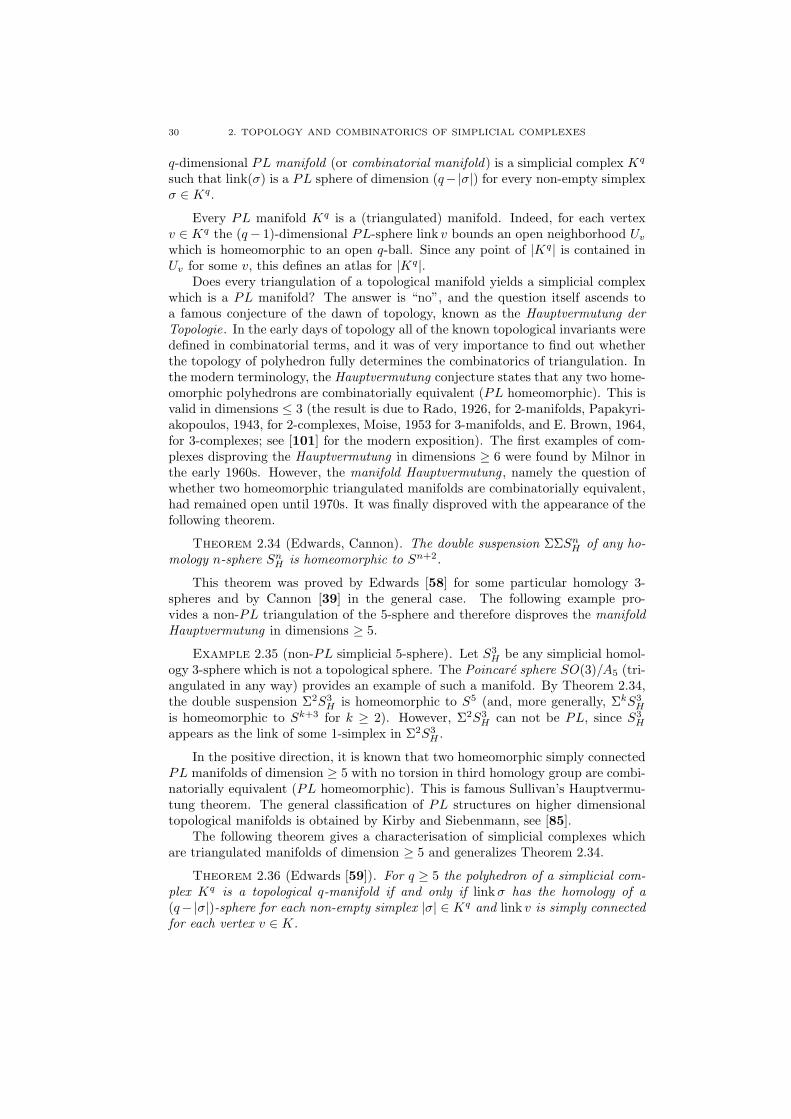
30 2. TOPOLOGY AND COMBINATORICS OF SIMPLICIAL COMPLEXES
q-dimensional PL manifold (or combinatorial manifold) is a simplicial complex Kq
such that link(σ) is a PL sphere of dimension (q−|σ|) for every non-empty simplexσ ∈ Kq.
Every PL manifold Kq is a (triangulated) manifold. Indeed, for each vertexv ∈ Kq the (q− 1)-dimensional PL-sphere link v bounds an open neighborhood Uv
which is homeomorphic to an open q-ball. Since any point of |Kq| is contained inUv for some v, this defines an atlas for |Kq|.
Does every triangulation of a topological manifold yields a simplicial complexwhich is a PL manifold? The answer is “no”, and the question itself ascends toa famous conjecture of the dawn of topology, known as the Hauptvermutung derTopologie. In the early days of topology all of the known topological invariants weredefined in combinatorial terms, and it was of very importance to find out whetherthe topology of polyhedron fully determines the combinatorics of triangulation. Inthe modern terminology, the Hauptvermutung conjecture states that any two home-omorphic polyhedrons are combinatorially equivalent (PL homeomorphic). This isvalid in dimensions ≤ 3 (the result is due to Rado, 1926, for 2-manifolds, Papakyri-akopoulos, 1943, for 2-complexes, Moise, 1953 for 3-manifolds, and E. Brown, 1964,for 3-complexes; see [101] for the modern exposition). The first examples of com-plexes disproving the Hauptvermutung in dimensions ≥ 6 were found by Milnor inthe early 1960s. However, the manifold Hauptvermutung , namely the question ofwhether two homeomorphic triangulated manifolds are combinatorially equivalent,had remained open until 1970s. It was finally disproved with the appearance of thefollowing theorem.
Theorem 2.34 (Edwards, Cannon). The double suspension ΣΣSnH of any ho-
mology n-sphere SnH is homeomorphic to Sn+2.
This theorem was proved by Edwards [58] for some particular homology 3-spheres and by Cannon [39] in the general case. The following example pro-vides a non-PL triangulation of the 5-sphere and therefore disproves the manifoldHauptvermutung in dimensions ≥ 5.
Example 2.35 (non-PL simplicial 5-sphere). Let S3H be any simplicial homol-
ogy 3-sphere which is not a topological sphere. The Poincare sphere SO(3)/A5 (tri-angulated in any way) provides an example of such a manifold. By Theorem 2.34,the double suspension Σ2S3
H is homeomorphic to S5 (and, more generally, ΣkS3H
is homeomorphic to Sk+3 for k ≥ 2). However, Σ2S3H can not be PL, since S3
H
appears as the link of some 1-simplex in Σ2S3H .
In the positive direction, it is known that two homeomorphic simply connectedPL manifolds of dimension ≥ 5 with no torsion in third homology group are combi-natorially equivalent (PL homeomorphic). This is famous Sullivan’s Hauptvermu-tung theorem. The general classification of PL structures on higher dimensionaltopological manifolds is obtained by Kirby and Siebenmann, see [85].
The following theorem gives a characterisation of simplicial complexes whichare triangulated manifolds of dimension ≥ 5 and generalizes Theorem 2.34.
Theorem 2.36 (Edwards [59]). For q ≥ 5 the polyhedron of a simplicial com-plex Kq is a topological q-manifold if and only if linkσ has the homology of a(q−|σ|)-sphere for each non-empty simplex |σ| ∈ Kq and link v is simply connectedfor each vertex v ∈ K.
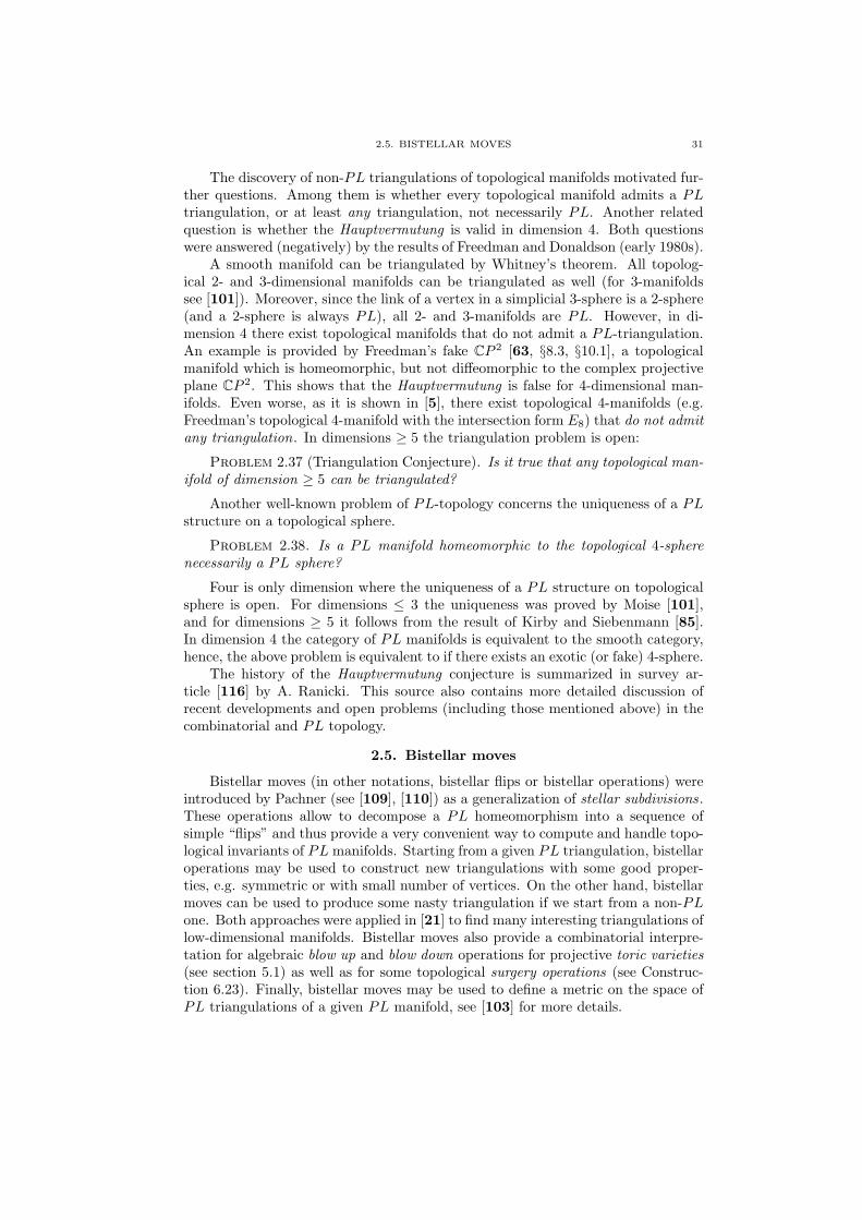
2.5. BISTELLAR MOVES 31
The discovery of non-PL triangulations of topological manifolds motivated fur-ther questions. Among them is whether every topological manifold admits a PLtriangulation, or at least any triangulation, not necessarily PL. Another relatedquestion is whether the Hauptvermutung is valid in dimension 4. Both questionswere answered (negatively) by the results of Freedman and Donaldson (early 1980s).
A smooth manifold can be triangulated by Whitney’s theorem. All topolog-ical 2- and 3-dimensional manifolds can be triangulated as well (for 3-manifoldssee [101]). Moreover, since the link of a vertex in a simplicial 3-sphere is a 2-sphere(and a 2-sphere is always PL), all 2- and 3-manifolds are PL. However, in di-mension 4 there exist topological manifolds that do not admit a PL-triangulation.An example is provided by Freedman’s fake CP 2 [63, §8.3, §10.1], a topologicalmanifold which is homeomorphic, but not diffeomorphic to the complex projectiveplane CP 2. This shows that the Hauptvermutung is false for 4-dimensional man-ifolds. Even worse, as it is shown in [5], there exist topological 4-manifolds (e.g.Freedman’s topological 4-manifold with the intersection form E8) that do not admitany triangulation. In dimensions ≥ 5 the triangulation problem is open:
Problem 2.37 (Triangulation Conjecture). Is it true that any topological man-ifold of dimension ≥ 5 can be triangulated?
Another well-known problem of PL-topology concerns the uniqueness of a PLstructure on a topological sphere.
Problem 2.38. Is a PL manifold homeomorphic to the topological 4-spherenecessarily a PL sphere?
Four is only dimension where the uniqueness of a PL structure on topologicalsphere is open. For dimensions ≤ 3 the uniqueness was proved by Moise [101],and for dimensions ≥ 5 it follows from the result of Kirby and Siebenmann [85].In dimension 4 the category of PL manifolds is equivalent to the smooth category,hence, the above problem is equivalent to if there exists an exotic (or fake) 4-sphere.
The history of the Hauptvermutung conjecture is summarized in survey ar-ticle [116] by A. Ranicki. This source also contains more detailed discussion ofrecent developments and open problems (including those mentioned above) in thecombinatorial and PL topology.
2.5. Bistellar moves
Bistellar moves (in other notations, bistellar flips or bistellar operations) wereintroduced by Pachner (see [109], [110]) as a generalization of stellar subdivisions.These operations allow to decompose a PL homeomorphism into a sequence ofsimple “flips” and thus provide a very convenient way to compute and handle topo-logical invariants of PL manifolds. Starting from a given PL triangulation, bistellaroperations may be used to construct new triangulations with some good proper-ties, e.g. symmetric or with small number of vertices. On the other hand, bistellarmoves can be used to produce some nasty triangulation if we start from a non-PLone. Both approaches were applied in [21] to find many interesting triangulations oflow-dimensional manifolds. Bistellar moves also provide a combinatorial interpre-tation for algebraic blow up and blow down operations for projective toric varieties(see section 5.1) as well as for some topological surgery operations (see Construc-tion 6.23). Finally, bistellar moves may be used to define a metric on the space ofPL triangulations of a given PL manifold, see [103] for more details.
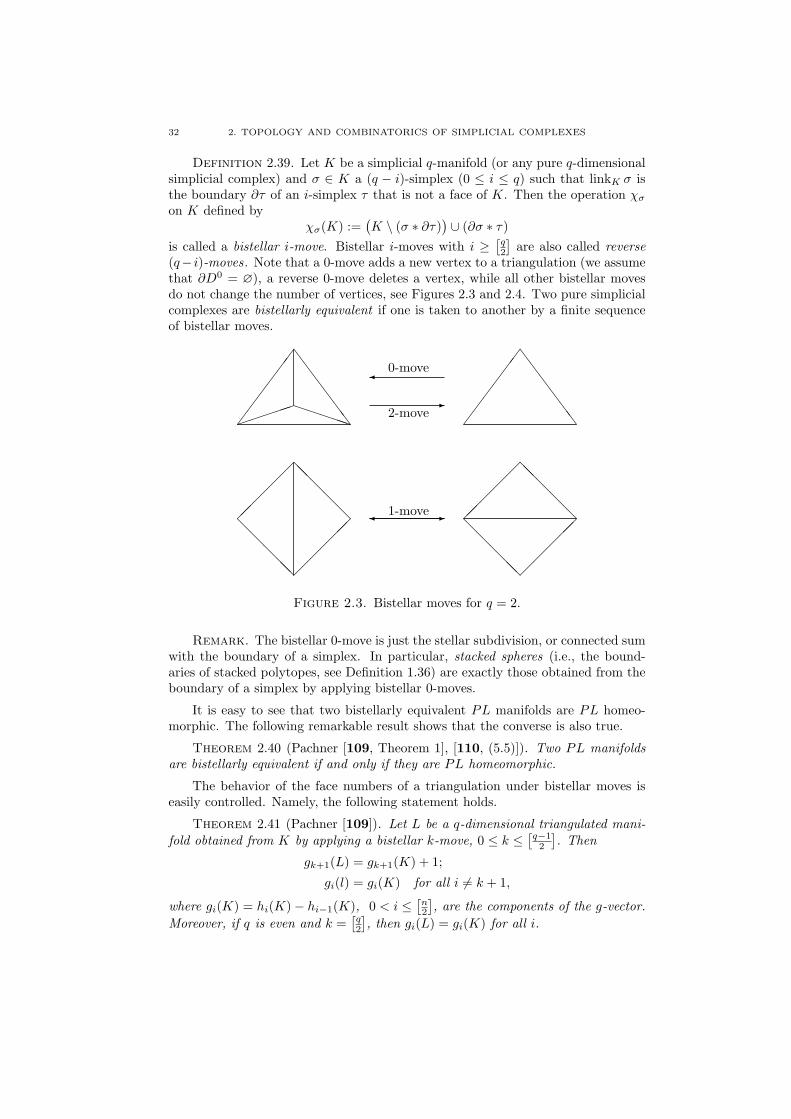
32 2. TOPOLOGY AND COMBINATORICS OF SIMPLICIAL COMPLEXES
Definition 2.39. Let K be a simplicial q-manifold (or any pure q-dimensionalsimplicial complex) and σ ∈ K a (q − i)-simplex (0 ≤ i ≤ q) such that linkK σ isthe boundary ∂τ of an i-simplex τ that is not a face of K. Then the operation χσ
on K defined byχσ(K) :=
(K \ (σ ∗ ∂τ)
) ∪ (∂σ ∗ τ)is called a bistellar i-move. Bistellar i-moves with i ≥ [
q2
]are also called reverse
(q− i)-moves. Note that a 0-move adds a new vertex to a triangulation (we assumethat ∂D0 = ∅), a reverse 0-move deletes a vertex, while all other bistellar movesdo not change the number of vertices, see Figures 2.3 and 2.4. Two pure simplicialcomplexes are bistellarly equivalent if one is taken to another by a finite sequenceof bistellar moves.
@@
@@@¡
¡¡
¡¡@
@@
@@¡¡
¡¡¡ -¾ 1-move
@@
@@@¡
¡¡
¡¡@
@@
@@¡¡
¡¡¡
¶¶
¶¶
¶¶S
SS
SSS³³³³³PPPPP
¾ 0-move
-2-move ¶
¶¶
¶¶¶S
SS
SSS
Figure 2.3. Bistellar moves for q = 2.
Remark. The bistellar 0-move is just the stellar subdivision, or connected sumwith the boundary of a simplex. In particular, stacked spheres (i.e., the bound-aries of stacked polytopes, see Definition 1.36) are exactly those obtained from theboundary of a simplex by applying bistellar 0-moves.
It is easy to see that two bistellarly equivalent PL manifolds are PL homeo-morphic. The following remarkable result shows that the converse is also true.
Theorem 2.40 (Pachner [109, Theorem 1], [110, (5.5)]). Two PL manifoldsare bistellarly equivalent if and only if they are PL homeomorphic.
The behavior of the face numbers of a triangulation under bistellar moves iseasily controlled. Namely, the following statement holds.
Theorem 2.41 (Pachner [109]). Let L be a q-dimensional triangulated mani-fold obtained from K by applying a bistellar k-move, 0 ≤ k ≤ [
q−12
]. Then
gk+1(L) = gk+1(K) + 1;
gi(l) = gi(K) for all i 6= k + 1,
where gi(K) = hi(K)− hi−1(K), 0 < i ≤ [n2
], are the components of the g-vector.
Moreover, if q is even and k =[q2
], then gi(L) = gi(K) for all i.
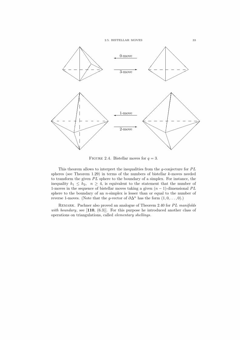
2.5. BISTELLAR MOVES 33
@@
@@
@@
@@¡¡
¡¡
¡¡
¡¡@
@@
@@
@@@¡
¡¡
¡¡
¡¡¡
³³³³³³³³³
BBBBB
HHHHHH-
2-move
¾ 1-move
@@
@@
@@
@@¡¡
¡¡
¡¡
¡¡@
@@
@@
@@@¡
¡¡
¡¡
¡¡¡
³³³³³³³³³
BBBBB
HHHHHH
©©©©©©
QQQ
@@
@@
@@
¶¶
¶¶
¶¶
HHHJ
JJ
JJ
-3-move
¾ 0-move
©©©©©©
QQQ
@@
@@
@@
¶¶
¶¶
¶¶
Figure 2.4. Bistellar moves for q = 3.
This theorem allows to interpret the inequalities from the g-conjecture for PLspheres (see Theorem 1.29) in terms of the numbers of bistellar k-moves neededto transform the given PL sphere to the boundary of a simplex. For instance, theinequality h1 ≤ h2, n ≥ 4, is equivalent to the statement that the number of1-moves in the sequence of bistellar moves taking a given (n − 1)-dimensional PLsphere to the boundary of an n-simplex is lesser than or equal to the number ofreverse 1-moves. (Note that the g-vector of ∂∆n has the form (1, 0, . . . , 0).)
Remark. Pachner also proved an analogue of Theorem 2.40 for PL manifoldswith boundary , see [110, (6.3)]. For this purpose he introduced another class ofoperations on triangulations, called elementary shellings.

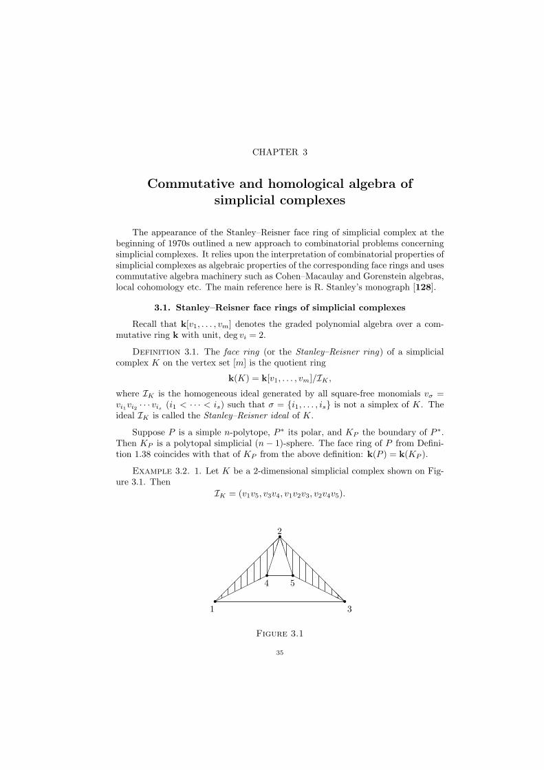
CHAPTER 3
Commutative and homological algebra ofsimplicial complexes
The appearance of the Stanley–Reisner face ring of simplicial complex at thebeginning of 1970s outlined a new approach to combinatorial problems concerningsimplicial complexes. It relies upon the interpretation of combinatorial properties ofsimplicial complexes as algebraic properties of the corresponding face rings and usescommutative algebra machinery such as Cohen–Macaulay and Gorenstein algebras,local cohomology etc. The main reference here is R. Stanley’s monograph [128].
3.1. Stanley–Reisner face rings of simplicial complexes
Recall that k[v1, . . . , vm] denotes the graded polynomial algebra over a com-mutative ring k with unit, deg vi = 2.
Definition 3.1. The face ring (or the Stanley–Reisner ring) of a simplicialcomplex K on the vertex set [m] is the quotient ring
k(K) = k[v1, . . . , vm]/IK ,
where IK is the homogeneous ideal generated by all square-free monomials vσ =vi1vi2 · · · vis (i1 < · · · < is) such that σ = i1, . . . , is is not a simplex of K. Theideal IK is called the Stanley–Reisner ideal of K.
Suppose P is a simple n-polytope, P ∗ its polar, and KP the boundary of P ∗.Then KP is a polytopal simplicial (n− 1)-sphere. The face ring of P from Defini-tion 1.38 coincides with that of KP from the above definition: k(P ) = k(KP ).
Example 3.2. 1. Let K be a 2-dimensional simplicial complex shown on Fig-ure 3.1. Then
IK = (v1v5, v3v4, v1v2v3, v2v4v5).
¡¡
¡¡
¡¡
¡¡
©©©©©©
@@
@@
@@
@@
£££££
BB
BBB
HHHHHHr
r r
r
r1 3
2
4 5
Figure 3.1
35
36 3. COMMUTATIVE AND HOMOLOGICAL ALGEBRA OF SIMPLICIAL COMPLEXES
2. The Stanley–Reisner ring k(K) is a quadratic algebra (i.e. the ideal IK isgenerated by quadratic monomials) if and only if K is a flag complex (see Defini-tion 2.18 and compare with Proposition 2.19).
3. Let K1 ∗K2 be the join of K1 and K2 (see Construction 2.9). Then
k(K1 ∗K2) = k(K1)⊗ k(K2).
In particular, for any two simple polytopes P1 and P2 we have
k(P1 × P2) = k(P1)⊗ k(P2)
(see Construction 1.12).4. Let K1 #σ1,σ2 K2 be the connected sum of two pure (n − 1)-dimensional
simplicial complexes on sets S1, S2 respectively, regarded as a simplicial complex onthe set S1 ∪σ S2 (see Construction 2.12). Then the ideal IK1#σ1,σ2K2 is generatedby the ideals IK1 , IK2 and the monomials vσ and vi1vi2 , where i1 ∈ S1 \ σ1 andi2 ∈ S2 \ σ2.
For any subset σ = i1, . . . , ik ⊂ [m] denote by vσ the square-free monomialvi1 · · · vik
. Note that the ideal IK is monomial and has basis of monomials vσ
corresponding to missing faces σ of K.
Proposition 3.3. Every square-free monomial ideal in the polynomial ring hasthe form IK for some simplicial complex K.
Proof. Let I be a square-free monomial ideal. Set
K = σ ⊂ [m] : vσ /∈ I.Then one easily checks that K is a simplicial complex and I = IK . ¤
Proposition 3.4. Let φ : K1 → K2 be a simplicial map (see Definition 2.7)between two simplicial complexes K1 and K2 on the vertex sets [m1] and [m2]respectively. Define the map φ∗ : k[w1, . . . , wm2 ] → k[v1, . . . , vm1 ] by
φ∗(wj) :=∑
i∈f−1jvi.
Then φ∗ descends to a homomorphism k(K2) → k(K1) (which we will also denoteby φ∗).
Proof. We have to check that φ∗(IK2) ⊂ IK1 . Suppose τ = j1, . . . , js ⊂[m2] is not a simplex of K2. Then
(3.1) φ∗(wj1 · · ·wjs) =∑
i1∈φ−1j1,...,is∈φ−1jsvi1 · · · vis .
We claim that σ = i1, . . . , is is not a simplex of K1 for any monomial vi1 · · · vis
in the right hand side of the above identity. Indeed, otherwise we would haveφ(σ) = τ ∈ K2 by the definition of simplicial map, which is impossible. Hence, theright hand side of (3.1) is in IK1 . ¤
Example 3.5. The face ring of the barycentric subdivision K ′ of K is
k(K ′) = k[bσ : σ ∈ K]/IK′ ,
3.1. STANLEY–REISNER FACE RINGS OF SIMPLICIAL COMPLEXES 37
where bσ is the polynomial generator corresponding to simplex σ ∈ K. We havethe simplicial map ∇ : K ′ → K (see Example 2.16). Then it is easy to see that
∇∗(vj) :=∑
σ∈K: min σ=j
bσ.
for any generator vj ∈ k(K).
Example 3.6. The non-degenerate map K ′ → ∆n−1 from Example 2.15 in-duces the following map of the corresponding Stanley–Reisner rings:
k[v1, . . . , vn] −→ k(K ′)
vi −→∑
|σ|=i
bσ.
This defines a canonical k[v1, . . . , vn]-module structure in k(K ′).
Definition 3.7. Let M = M0 ⊕M1 ⊕ . . . be a graded k-module. The series
F (M ; t) =∞∑
i=0
(dimk M i)ti
is called the Poincare series of M .
Remark. In the algebraic literature the series F (M ; t) is called the Hilbertseries or Hilbert–Poincare series.
The following lemma may be considered as an algebraic definition of the h-vector of a simplicial complex.
Lemma 3.8 (Stanley [128, Theorem II.1.4]). The Poincare series of k(Kn−1)can be calculated as
F(k(Kn−1); t
)=
n−1∑
i=−1
fit2(i+1)
(1− t2)i+1=
h0 + h1t2 + · · ·+ hnt2n
(1− t2)n,
where (f0, . . . , fn−1) is the f -vector and (h0, . . . , hn) is the h-vector of Kn−1.
Proof. Any monomial in k(Kn−1) has the form vα1i1· · · vαk+1
ik+1, where
i1, . . . , ik+1 is a simplex of Kn−1 and α1, . . . , αk+1 are some positive integers.Thus, every k-simplex of Kn−1 contributes the summand t2(k+1)
(1−t2)k+1 to the Poincareseries, which proves the first identity. The second identity is an obvious corollaryof (1.8). ¤
Example 3.9. 1. Let K = ∆n. Then fi =(n+1i+1
)for −1 ≤ i ≤ n, h0 = 1 and
hi = 0 for i > 0. Since any subset of [n + 1] is a simplex of ∆n, we have k(∆n) =k[v1, . . . , vn+1] and F (k(∆n); t) = (1− t2)−(n+1), which agrees with Lemma 3.8.
2. Let K be the boundary of an n-simplex. Then hi = 1, i = 0, 1, . . . , n, andk(K) = k[v1, . . . , vn+1]/(v1v2 · · · vn+1). By Lemma 3.8,
F(k(K); t
)=
1 + t2 + · · ·+ t2n
(1− t2)n.
38 3. COMMUTATIVE AND HOMOLOGICAL ALGEBRA OF SIMPLICIAL COMPLEXES
3.2. Cohen–Macaulay rings and complexes
Here we suppose k is a field. Let A be a finitely-generated commutative gradedalgebra over k. We also assume that A has only even-degree graded components,so it is commutative in both usual and graded sense.
Definition 3.10. The Krull dimension of A (denoted Kd A) is the maxi-mal number of algebraically independent elements of A. A sequence θ1, . . . , θn ofn = Kd A homogeneous elements of A is called a hsop (homogeneous system of pa-rameters) if the Krull dimension of the quotient A/(θ1, . . . , θn) is zero. Equivalently,θ1, . . . , θn is a hsop if n = Kd A and A is a finitely-generated k[θ1, . . . , θn]-module.The elements of a hsop are algebraically independent.
Lemma 3.11 (Noether normalization lemma). For any finitely-generated gra-ded algebra A there exists a hsop. If k is of zero characteristic and A is generatedby degree-two elements, then a degree-two hsop can be chosen.
In the case when A is generated by degree-two elements, a degree-two hsop iscalled a lsop (linear system of parameters).
Remark. If k is of finite characteristic then a lsop may fail to exist for algebrasgenerated in degree two, see Example 5.26 below.
In the rest of this chapter we assume that the field k is of zero characteristic.
Definition 3.12. A sequence θ1, . . . , θk of homogeneous elements of A is calleda regular sequence if θi+1 is not a zero divisor in A/(θ1, . . . , θi) for 0 ≤ i < k (i.e.the multiplication by θi+1 is a monomorphism of A/(θ1, . . . , θi) into itself). Equiv-alently, θ1, . . . , θk is a regular sequence if θ1, . . . , θk are algebraically independentand A is a free k[θ1, . . . , θk]-module.
Remark. The concept of a regular sequence can be extended to non-finitely-generated graded algebras and to algebras over any integral domain. Regular se-quences in graded polynomial rings R[a1, a2, . . . , ] on infinitely many generators,where deg ai = −2i and R is a subring of the field Q of rationals, are used in thealgebraic topology for constructing complex cobordism theories with coefficients,see [89].
Any two maximal regular sequences have the same length, which is called thedepth of A and denoted depth A. Obviously, depth A ≤ Kd A.
Definition 3.13. Algebra A is called Cohen–Macaulay if it admits a regularsequence θ1, . . . , θn of length n = Kd A.
A regular sequence θ1, . . . , θn of length n = Kd A is a hsop. It follows that A isCohen–Macaulay if and only if there exists a hsop θ1, . . . , θn such that A is a freek[θ1, . . . , θn]-module. If in addition A is generated by degree-two elements, thenone can choose θ1, . . . , θn to be a lsop. In this case the following formula for thePoincare series of A holds
F (A; t) =F
(A/(θ1, . . . , θn); t
)
(1− t2)n,
where F (A/(θ1, . . . , θn); t) = h0 + h1t2 + · · · is a polynomial. The finite vector
(h0, h1, . . .) is called the h-vector of A.
3.2. COHEN–MACAULAY RINGS AND COMPLEXES 39
Definition 3.14. A simplicial complex Kn−1 is called Cohen–Macaulay (overk) if its face ring k(Kn−1) is Cohen–Macaulay.
Obviously, Kdk(Kn−1) = n. Lemma 3.8 shows that the h-vector of k(K)coincides with the h-vector of K.
Example 3.15. Let K1 be the boundary of a 2-simplex. Then k(K1) =k[v1, v2, v3]/(v1v2v3). The elements v1, v2 ∈ k(K) are algebraically independent,but do not form a hsop, since k(K)/(v1, v2) ∼= k[v3] and Kdk(K)/(v1, v2) = 1 6= 0.On the other hand, the elements θ1 = v1 − v3, θ2 = v2 − v3 of k(K) form a hsop,since k(K)/(θ1, θ2) ∼= k[t]/t3. It is easy to see that k(K) is a free k[θ1, θ2]-modulewith one 0-dimensional generator 1, one 1-dimensional generator v1, and one 2-dimensional generator v2
1 . Thus, k(K) is Cohen–Macaulay and (θ1, θ2) is a regularsequence.
Theorem 3.16 (Stanley). If Kn−1 is a Cohen–Macaulay simplicial complex,then h(Kn−1) = (h0, . . . , hn) is an M -vector (see Definition 1.31).
Proof. Let θ1, . . . , θn be a regular sequence of degree-two elements of k(K).Then A = k(K)/(θ1, . . . , θn) is a graded algebra generated by degree-two elements,and dimk A2i = hi. Now the result follows from Theorem 1.32. ¤
The following fundamental theorem characterizes Cohen–Macaulay complexescombinatorially.
Theorem 3.17 (Reisner [117]). A simplicial complex K is Cohen–Macaulayover k if and only if for any simplex σ ∈ K (including σ = ∅) and i < dim(link σ),Hi(link σ;k) = 0. (Here Hi(X;k) denotes the i-th reduced homology group of Xwith coefficients in k.)
Corollary 3.18. A simplicial sphere is a Cohen–Macaulay complex.
Theorem 3.16 shows that the h-vector of a simplicial sphere is an M -vector.This argument was used by Stanley to extend the UBC (Theorem 1.33) to simplicialspheres.
Corollary 3.19 (Upper Bound Theorem for spheres, Stanley [123]). The h-vector (h0, h1, . . . , hn) of a simplicial (n− 1)-sphere Kn−1 with m vertices satisfies
hi(Kn−1) ≤ (m−n+i−1
i
), 0 ≤ i <
[n2
].
Hence, the UBC holds for simplicial spheres, that is,
fi(Kn−1) ≤ fi
(Cn(m)
)for i = 2, . . . , n− 1.
(see Corollary 1.35).
Proof. Since h(Kn−1) is an M -vector, there exists a graded algebra A =A0 ⊕ A2 ⊕ · · · ⊕ A2n generated by degree-two elements such that dimk A2i = hi
(Theorem 1.32). In particular, dimk A2 = h1 = m−n. Since A is generated by A2,the number hi can not exceed the total number of monomials of degree i in (m−n)variables. The latter is exactly
(m−n+i−1
i
). ¤
40 3. COMMUTATIVE AND HOMOLOGICAL ALGEBRA OF SIMPLICIAL COMPLEXES
3.3. Homological algebra background
Here we review some homology algebra. Unless otherwise stated, all modulesin this section are assumed to be finitely-generated graded k[v1, . . . , vm]-modules,deg vi = 2.
Definition 3.20. A finite free resolution of a module M is an exact sequence
(3.2) 0 → R−h d−→ R−h+1 d−→ · · · −→ R−1 d−→ R0 d−→ M → 0,
where the R−i are finitely-generated free modules and the maps d are degree-preserving. The minimal number h for which a free resolution (3.2) exists is calledthe homological dimension of M and denoted hdM . By the Hilbert syzygy theorema finite free resolution (3.2) exists and hdM ≤ m. A resolution (3.2) can be writtenas a free bigraded differential module [R, d], where R =
⊕R−i,j , R−i,j := (R−i)j
(the j-th graded component of the free module R−i). The cohomology of [R, d]is zero in non-zero dimensions and H0[R, d] = M . Conversely, a free bigradeddifferential module [R =
⊕i,j≥0 R−i,j , d : R−i,j → R−i+1,j ] with H0[R, d] = M
and H−i[R, d] = 0 for i > 0 defines a free resolution (3.2) with R−i := R−i,∗ =⊕j R−i,j .
Remark. For the reasons specified below we numerate the terms of a freeresolution by non-positive numbers, thereby viewing it as a cochain complex.
The Poincare series of M can be calculated from any free resolution (3.2) bymeans of the following classical theorem.
Theorem 3.21. Suppose that R−i has rank qi with free generators in degreesd1i, . . . , dqii, i = 1, . . . , h. Then
(3.3) F (M ; t) = (1− t2)−mh∑
i=0
(−1)i(td1i + · · ·+ tdqii).
Proof. By the definition of resolution, the following map of cochain complexes
0 −−−−→ R−h d−−−−→ R−h+1 d−−−−→ · · · d−−−−→ R−1 d−−−−→ R0 −−−−→ 0yy
yy
0 −−−−→ 0 −−−−→ 0 −−−−→ · · · −−−−→ 0 −−−−→ M −−−−→ 0is a quasi-isomorphism, i.e. induces an isomorphism in the cohomology. Equatingthe Euler characteristics of both complexes in each degree we get (3.3) ¤
Construction 3.22. There is the following straightforward way to constructa free resolution for a module M . Take a set of generators a1, . . . , ak0 for M anddefine R0 to be a free k[v1, . . . , vm]-module with k0 generators in the correspondingdegrees. There is an obvious epimorphism R0 → M . Then take a set of generatorsa1, . . . , ak1 in the kernel of R0 → M and define R−1 to be a free k[v1, . . . , vm]-module with k1 generators in the corresponding degrees, and so on. On the i-thstep we take a set of generators in the kernel of the previously constructed mapd : R−i+1 → R−i+2 and define R−i to be a free module with the correspondinggenerators. The Hilbert syzygy theorem guarantees this process to end up at mostat the m-th step.
3.3. HOMOLOGICAL ALGEBRA BACKGROUND 41
Example 3.23 (minimal resolution). For graded finitely generated modulesM a minimal generator set (or a minimal basis) can be chosen. This is done asfollows. Take the lowest degree in which M is non-zero and there choose a vectorspace basis. Span a module M1 by this basis and then take the lowest degree inwhich M 6= M1. In this degree choose a vector space basis in the complement ofM1, and span a module M2 by this basis and M1. Then continue this process.Since M is finitely generated, on some p-th step we get M = Mp and a basis for Mwith minimal number of generators.
If we take a minimal set of generators for modules at each step of Construc-tion 3.22, then the produced resolution is called minimal . Each of its termsR−i has the smallest possible rank (see Example 3.26 below). There is also thefollowing more formal (but less convenient for particular computations) defini-tion of minimal resolution (see [2]). Let M , M ′ be two modules. Set J (M) =v1M + v2M + · · · + vmM ⊂ M . A map f : M → M ′ is called minimal ifKer f ⊂ J (M). A resolution (3.2) is called minimal if all maps d are minimal.A minimal resolution is unique up to an isomorphism.
Example 3.24 (Koszul resolution). Let M = k. The k[v1, . . . , vm]-modulestructure on k is defined via the map k[v1, . . . , vm] → k that sends each vi to 0.Let Λ[u1, . . . , um] denote the exterior algebra on m generators. Turn the tensorproduct R = Λ[u1, . . . , um] ⊗ k[v1, . . . , vm] (here and below we use ⊗ for ⊗k) intoa differential bigraded algebra by setting
bideg ui = (−1, 2), bideg vi = (0, 2),
dui = vi, dvi = 0,(3.4)
and requiring that d be a derivation of algebras. An explicit construction of cochainhomotopy [92, §7.2] shows that H−i[R, d] = 0 for i > 0 and H0[R, d] = k. SinceΛ[u1, . . . , um] ⊗ k[v1, . . . , vm] is a free k[v1, . . . , vm]-module, it determines a freeresolution of k. This resolution is known as the Koszul resolution. Its expandedform is as follows:
0 → Λm[u1, . . . , um]⊗ k[v1, . . . , vm] −→ · · ·−→ Λ1[u1, . . . , um]⊗ k[v1, . . . , vm] −→ k[v1, . . . , vm] −→ k → 0,
where Λi[u1, . . . , um] is the submodule of Λ[u1, . . . , um] spanned by monomialsof length i. Thus, in the notations of (3.2) we have R−i = Λi[u1, . . . , um] ⊗k[v1, . . . , vm].
Let N be another module; then applying the functor ⊗k[v1,...,vm]N to (3.2) weobtain the following cochain complex of graded modules:
0 −→ R−h ⊗k[v1,...,vm] N −→ · · · −→ R0 ⊗k[v1,...,vm] N −→ 0
and the corresponding bigraded differential module [R ⊗ N, d]. The (−i)-th co-homology module of the above cochain complex is denoted Tor−i
k[v1,...,vm](M, N),i.e.
Tor−ik[v1,...,vm](M,N) := H−i[R⊗k[v1,...,vm] N, d]
=Ker[d : R−i ⊗k[v1,...,vm] N → R−i+1 ⊗k[v1,...,vm] N ]
d(R−i−1 ⊗k[v1,...,vm] N).
42 3. COMMUTATIVE AND HOMOLOGICAL ALGEBRA OF SIMPLICIAL COMPLEXES
Since both the R−i’s and N are graded modules, we actually have
Tor−ik[v1,...,vm](M, N) =
⊕
j
Tor−i,jk[v1,...,vm](M,N),
where
Tor−i,jk[v1,...,vm](M, N) =
Ker[d : (R−i ⊗k[v1,...,vm] N)j → (R−i+1 ⊗k[v1,...,vm] N)j
]
d(R−i−1 ⊗k[v1,...,vm] N)j.
The above modules combine to a bigraded k[v1, . . . , vm]-module,
Tork[v1,...,vm](M, N) =⊕
i,j
Tor−i,jk[v1,...,vm](M,N).
The following properties of Tor−ik[v1,...,vm](M, N) are well known (see e.g. [92]).
Proposition 3.25. (a) The module Tor−ik[v1,...,vm](M,N) does not depend, up
to isomorphism, on a choice of resolution (3.2).(b) Both Tor−i
k[v1,...,vm]( · , N) and Tor−ik[v1,...,vm](M, · ) are covariant functors.
(c) Tor0k[v1,...,vm](M, N) ∼= M ⊗k[v1,...,vm] N .(d) Tor−i
k[v1,...,vm](M, N) ∼= Tor−ik[v1,...,vm](N, M).
In the homological algebra A-modules TorA(M, N) are defined for algebras Afar more general than polynomial rings (and finitely-generatedness assumption formodules M and N may be also dropped). Although a finite A-free resolution (3.2)of M may fail to exist in general, there is always a projective resolution, which allowsto define TorA(M, N) in the same way as above. Note that projective modules overthe polynomial algebra are free. In the non-graded case this was known as the Serreproblem, now solved by Quillen and Suslin. However the graded version of this factis much easier to prove. In this text the Tor-modules TorA(M, N) over algebrasdifferent from the polynomial ring appear only in sections 7.1 and 8.3.
3.4. Homological properties of face rings: Tor-algebras and Bettinumbers
Here we apply general constructions from the previous section in the case whenM = k(K) and N = k. As usual, K = Kn−1 is assumed to be a simplicial complexon [m]. Since deg vi = 2, we have
Tork[v1,...,vm]
(k(K),k
)=
m⊕
i,j=0
Tor−i,2jk[v1,...,vm]
(k(K),k
)
(i.e. Tork[v1,...,vm](k(K),k) is non-zero only in even second degrees). Define thebigraded Betti numbers of k(K) by
(3.5) β−i,2j(k(K)
):= dimk Tor−i,2j
k[v1,...,vm]
(k(K),k
), 0 ≤ i, j ≤ m.
Suppose that (3.2) is a minimal free resolution of M = k(K) (Example 3.23). ThenR0 ∼= k[v1, . . . , vm] is a free k[v1, . . . , vm]-module with one generator of degree 0.The basis of R−1 is a minimal generator set for IK = Ker[k[v1, . . . , vm] → k(K)]and is represented by the missing faces of K. For each missing face i1, . . . , ik of Kdenote by vi1,...,ik
the corresponding basis element of R−1. Then deg vi1,...,ik= 2k
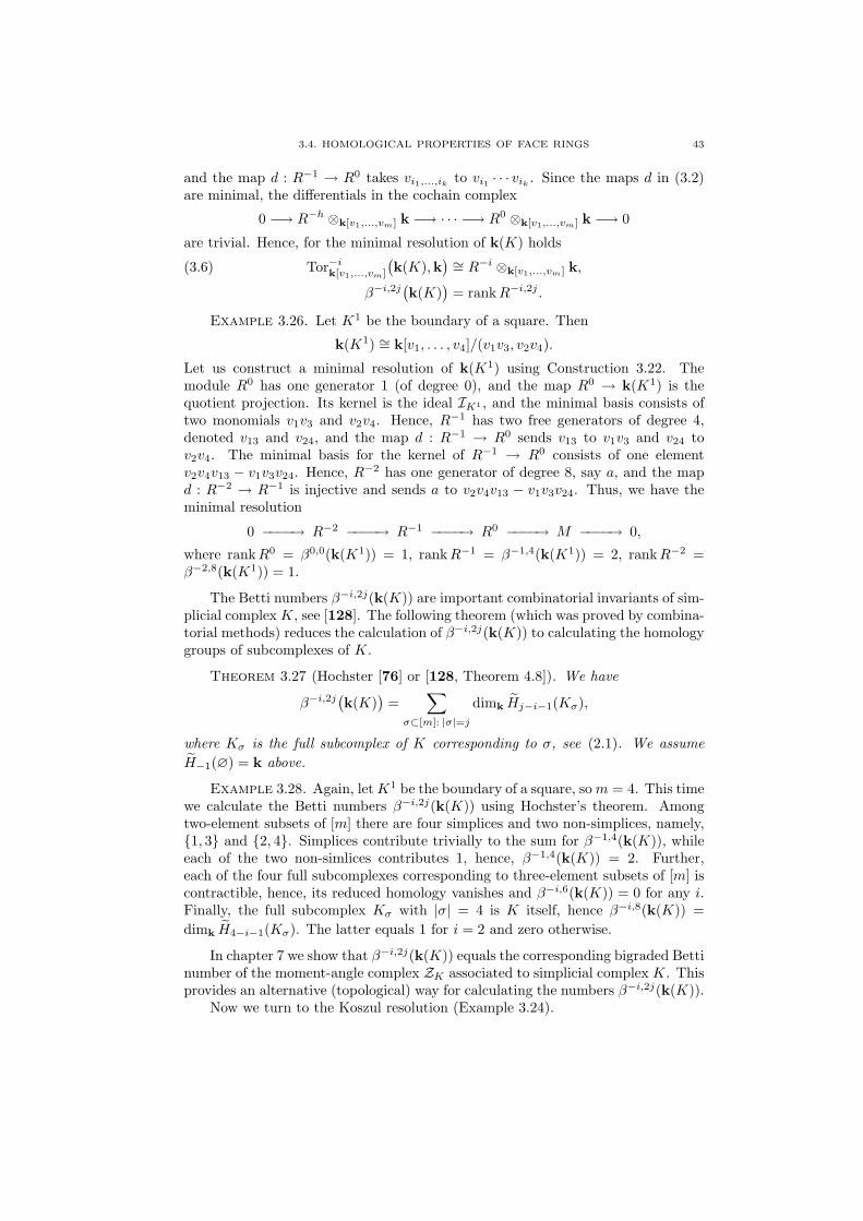
3.4. HOMOLOGICAL PROPERTIES OF FACE RINGS 43
and the map d : R−1 → R0 takes vi1,...,ikto vi1 · · · vik
. Since the maps d in (3.2)are minimal, the differentials in the cochain complex
0 −→ R−h ⊗k[v1,...,vm] k −→ · · · −→ R0 ⊗k[v1,...,vm] k −→ 0
are trivial. Hence, for the minimal resolution of k(K) holds
Tor−ik[v1,...,vm]
(k(K),k
) ∼= R−i ⊗k[v1,...,vm] k,(3.6)
β−i,2j(k(K)
)= rank R−i,2j .
Example 3.26. Let K1 be the boundary of a square. Then
k(K1) ∼= k[v1, . . . , v4]/(v1v3, v2v4).
Let us construct a minimal resolution of k(K1) using Construction 3.22. Themodule R0 has one generator 1 (of degree 0), and the map R0 → k(K1) is thequotient projection. Its kernel is the ideal IK1 , and the minimal basis consists oftwo monomials v1v3 and v2v4. Hence, R−1 has two free generators of degree 4,denoted v13 and v24, and the map d : R−1 → R0 sends v13 to v1v3 and v24 tov2v4. The minimal basis for the kernel of R−1 → R0 consists of one elementv2v4v13 − v1v3v24. Hence, R−2 has one generator of degree 8, say a, and the mapd : R−2 → R−1 is injective and sends a to v2v4v13 − v1v3v24. Thus, we have theminimal resolution
0 −−−−→ R−2 −−−−→ R−1 −−−−→ R0 −−−−→ M −−−−→ 0,
where rank R0 = β0,0(k(K1)) = 1, rank R−1 = β−1,4(k(K1)) = 2, rank R−2 =β−2,8(k(K1)) = 1.
The Betti numbers β−i,2j(k(K)) are important combinatorial invariants of sim-plicial complex K, see [128]. The following theorem (which was proved by combina-torial methods) reduces the calculation of β−i,2j(k(K)) to calculating the homologygroups of subcomplexes of K.
Theorem 3.27 (Hochster [76] or [128, Theorem 4.8]). We have
β−i,2j(k(K)
)=
∑
σ⊂[m]: |σ|=j
dimk Hj−i−1(Kσ),
where Kσ is the full subcomplex of K corresponding to σ, see (2.1). We assumeH−1(∅) = k above.
Example 3.28. Again, let K1 be the boundary of a square, so m = 4. This timewe calculate the Betti numbers β−i,2j(k(K)) using Hochster’s theorem. Amongtwo-element subsets of [m] there are four simplices and two non-simplices, namely,1, 3 and 2, 4. Simplices contribute trivially to the sum for β−1,4(k(K)), whileeach of the two non-simlices contributes 1, hence, β−1,4(k(K)) = 2. Further,each of the four full subcomplexes corresponding to three-element subsets of [m] iscontractible, hence, its reduced homology vanishes and β−i,6(k(K)) = 0 for any i.Finally, the full subcomplex Kσ with |σ| = 4 is K itself, hence β−i,8(k(K)) =dimk H4−i−1(Kσ). The latter equals 1 for i = 2 and zero otherwise.
In chapter 7 we show that β−i,2j(k(K)) equals the corresponding bigraded Bettinumber of the moment-angle complex ZK associated to simplicial complex K. Thisprovides an alternative (topological) way for calculating the numbers β−i,2j(k(K)).
Now we turn to the Koszul resolution (Example 3.24).
44 3. COMMUTATIVE AND HOMOLOGICAL ALGEBRA OF SIMPLICIAL COMPLEXES
Lemma 3.29. For any module M holds
Tork[v1,...,vm](M,k) ∼= H[Λ[u1, . . . , um]⊗M, d
],
where H[Λ[u1, . . . , um]⊗M,d] is the cohomology of the bigraded differential moduleΛ[u1, . . . , um]⊗M and d is defined as in (3.4).
Proof. Using the Koszul resolution [Λ[u1, . . . , um] ⊗ k[v1, . . . , vm], d] in thedefinition of Tork[v1,...,vm](k,M), we calculate
Tork[v1,...,vm](M,k) ∼= Tork[v1,...,vm](k, M)
= H[Λ[u1, . . . , um]⊗ k[v1, . . . , vm]⊗k[v1,...,vm] M
] ∼= H[Λ[u1, . . . , um]⊗M
].
¤
Corollary 3.30. Suppose that a k[v1, . . . , vm]-module M is an algebra, thenTork[v1,...,vm](M,k) is canonically a finite-dimensional bigraded k-algebra.
Proof. It is easy to see that in this case the tensor product Λ[u1, . . . , um]⊗Mis a differential algebra, and Tork[v1,...,vm](M,k) is its cohomology by Lemma 3.29.
¤
Definition 3.31. The bigraded algebra Tork[v1,...,vm](M,k) is called the Tor-algebra of algebra M . If M = k(K) then it is called the Tor-algebra of simplicialcomplex K.
Remark. For general N 6= k the module Tork[v1,...,vm](M,N) has no canonicalmultiplicative structure even if both M and N are algebras.
Lemma 3.32. A simplicial map φ : K1 → K2 between two simplicial complexeson the vertex sets [m1] and [m2] respectively induces a homomorphism
(3.7) φ∗t : Tork[w1,...,wm2 ]
(k(K2),k
) → Tork[v1,...,vm1 ]
(k(K1),k
)
of the corresponding Tor-algebras.
Proof. This follows directly from propositions 3.4 and 3.25 (b). ¤
Construction 3.33 (multigraded structure in the Tor-algebra). We may in-vest the polynomial ring k[v1, . . . , vm] with a multigrading (more precisely, Nm-grading) by setting mdeg vi = (0, . . . , 0, 2, 0, . . . , 0) where 2 stands at the i-th place.Then the multidegree of monomial vi1
1 · · · vimm is (2i1, . . . , 2im). Suppose that al-
gebra M is a quotient of the polynomial ring by a monomial ideal. Then themultigraded structure descends to M and to the terms of resolution (3.2). We mayassume that the differentials in the resolution preserve the multidegrees. Then themodule Tork[v1,...,vm](M, N) acquires a canonical N⊕ Nm-grading, i.e.
Tork[v1,...,vm](M,k) =⊕
i≥0, j∈Nm
Tor−i,jk[v1,...,vm](M,k).
In particular, the Tor-algebra of K is canonically an N⊕ Nm-graded algebra.
Remark. According to our agreement, the first degree in the Tor-algebra isnon-positive. (Remember that we numerated the terms of k[v1, . . . , vm]-free Koszulresolution of k by non-positive integers.) In these notations the Koszul complex[M ⊗ Λ[u1, . . . , um], d] becomes a cochain complex, and Tork[v1,...,vm](M,k) is itscohomology , not the homology as usually regarded. One of the reasons for such an
3.4. HOMOLOGICAL PROPERTIES OF FACE RINGS 45
agreement is that Tork[v1,...,vm](k(K),k) is a contravariant functor from the cate-gory of simplicial complexes and simplicial maps, see Lemma 3.32. It also explainsour notation Tor∗,∗k[v1,...,vm](M,k), used instead of the usual Tork[v1,...,vm]
∗,∗ (M,k).These notations are convenient for working with Eilenberg–Moore spectral se-quences, see section 7.1.
The upper bound hdM ≤ m from the Hilbert syzygy theorem can be replacedby the following sharper result.
Theorem 3.34 (Auslander and Buchsbaum). hd M = m− depth M .
In particular, if M = k(Kn−1) and Kn−1 is Cohen–Macaulay (see Defini-tion 3.14), then hdk(K) = m− n and Tor−i
k[v1,...,vm](k(K),k) = 0 for i > m− n.¿From now on we assume that M is generated by degree-two elements and
the k[v1, . . . , vm]-module structure in M is defined through an epimorphism p :k[v1, . . . , vm] → M (both assumptions are satisfied by definition for M = k(K)).Suppose that θ1, . . . , θk is a regular sequence of degree-two elements of M . Let J :=(θ1, . . . , θk) ⊂ M be the ideal generated by θ1, . . . , θk. Choose degree-two elementsti ∈ k[v1, . . . , vm] such that p(ti) = θi, i = 1, . . . , k. The ideal in k[v1, . . . , vm]generated by t1, . . . , tk will be also denoted by J . Then we have k[v1, . . . , vm]/J ∼=k[w1, . . . , wm−k]. Under these assumptions we have the following reduction lemma.
Lemma 3.35. The following isomorphism of algebras holds for any ideal Jgenerated by a regular sequence:
Tork[v1,...,vm](M,k) = Tork[v1,...,vm]/J (M/J ,k).
In order to prove the lemma we need the following fact from the homologyalgebra.
Theorem 3.36 ([40, p. 349]). Let Λ be an algebra, Γ its subalgebra, and Ω =Λ//Γ the quotient algebra. Suppose that Λ is a free Γ-module and we are given anΩ-module A and a Λ-module C. Then there exists a spectral sequence Er, dr suchthat
Er ⇒ TorΛ(A,C), E2 = TorΩ(A, TorΓ(C,k)
).
Proof of Lemma 3.35. Set Λ = k[v1, . . . , vm], Γ = k[t1, . . . , tk], A = k, C =M . Then Λ is a free Γ-module and Ω = Λ//Γ = k[v1, . . . , vm]/J . Therefore,Theorem 3.36 gives a spectral sequence
Er ⇒ Tork[v1,...,vm](M,k), E2 = TorΩ(TorΓ(M,k),k
).
Since θ1, . . . , θk is a regular sequence, M is a free Γ-module. Therefore,
TorΓ(M,k) = M ⊗Γ k = M/J and TorqΓ(M,k) = 0 for q 6= 0.
It follows that Ep,q2 = 0 for q 6= 0. Thus, the spectral sequence collapses at the E2
term, and we have
Tork[v1,...,vm](M,k) = TorΩ(TorΓ(M,k),k
)= Tork[v1,...,vm]/J (M/J ,k),
which concludes the proof. ¤
46 3. COMMUTATIVE AND HOMOLOGICAL ALGEBRA OF SIMPLICIAL COMPLEXES
3.5. Gorenstein complexes and Dehn–Sommerville equations
It follows from Theorem 3.34 that if M is Cohen–Macaulay of Krull dimen-sion n, then depth M = n, hd M = m−n, and Tor−i
k[v1,...,vm](M,k) = 0 for i > m−n.
Definition 3.37. Suppose M is a Cohen–Macaulay algebra of Krull dimen-sion n. Then M is called a Gorenstein algebra if Tor−(m−n)
k[v1,...,vm](M,k) ∼= k.
Following Stanley [128], we call a simplicial complex K Gorenstein if k(K) isa Gorenstein algebra. Further, K is called Gorenstein* if k(K) is Gorenstein andK = core K (see Definition 2.24). The following theorem characterizes Gorenstein*simplicial complexes.
Theorem 3.38 ([128, §II.5]). A simplicial complex K is Gorenstein* over kif and only if for any simplex σ ∈ K (including σ = ∅) the subcomplex linkσ hasthe homology of a sphere of dimension dim(link σ).
In particular, simplicial spheres and simplicial homology spheres (triangulatedmanifolds with the homology of a sphere) are Gorenstein* complexes. However, theGorenstein* property does not guarantee a complex to be a triangulated manifold(links of vertices are not necessarily simply connected, compare with Theorem 2.36).The Poincare series of the Tor-algebra and the face ring of a Gorenstein* complexare “self dual” in the following sense.
Theorem 3.39 ([128, §II.5]). Suppose Kn−1 is a Gorenstein* complex. Thenthe following identities hold for the Poincare series of Tor−i
k[v1,...,vm](k(K),k), 0 ≤i ≤ m− n:
F(Tor−i
k[v1,...,vm]
(k(K),k
); t
)= t2mF
(Tor−(m−n)+i
k[v1,...,vm]
(k(K),k
); 1
t
).
Equivalently,
β−i,2j(k(K)
)= β−(m−n)+i,2(m−j)
(k(K)
), 0 ≤ i ≤ m− n, 0 ≤ j ≤ m.
Corollary 3.40. If Kn−1 is Gorenstein* then
F(k(K), t
)= (−1)nF
(k(K), 1
t
).
Proof. We apply Theorem 3.21 to a minimal resolution of k(K). It followsfrom (3.6) that the numerators of the summands in the right hand side of (3.3) areexactly F
(Tor−i
k[v1,...,vm](k(K),k); t), i = 1, . . . , m− n. Hence,
F(k(K); t
)= (1− t2)−m
m−n∑
i=0
(−1)iF(Tor−i
k[v1,...,vm]
(k(K),k
); t
).
Using Theorem 3.39, we calculate
F(k(K); t
)= (1− t2)−m
m−n∑
i=0
(−1)it2mF(Tor−(m−n)+i
k[v1,...,vm]
(k(K),k
); 1
t
)
=(1− ( 1
t )2)−m(−1)m
m−n∑
j=0
(−1)m−n−jF(Tor−j
k[v1,...,vm]
(k(K),k
); 1
t
)
= (−1)nF(k(K); 1
t
).
¤
3.5. GORENSTEIN COMPLEXES AND DEHN–SOMMERVILLE EQUATIONS 47
Corollary 3.41. The Dehn–Sommerville relations hi = hn−i, 0 ≤ i ≤ n, holdfor any Gorenstein* complex Kn−1 (in particular, for any simplicial sphere).
Proof. This follows from Lemma 3.8 and Corollary 3.40. ¤As it was pointed out by Stanley in [127], Gorenstein* complexes are the
most appropriate candidates for generalizing the g-theorem to. (As we have seen,polytopal spheres, PL spheres, simplicial spheres and simplicial homology spheresare examples of Gorenstein* complexes).
The Dehn–Sommerville equations can be generalized even beyond Gorenstein*complexes. In [86] Klee reproved the f -vector version (1.10) of the Dehn–Sommer-ville equations in the more general context of Eulerian complexes. (A pure simplicialcomplex Kn−1 is called Eulerian if for any simplex σ ∈ K, including ∅, holdsχ(link σ) = χ(Sn−|σ|−1) = 1 + (−1)n−|σ|−1.) Generalizations of equations (1.10)were obtained by Bayer and Billera [17] (for Eulerian posets) and Chen and Yan [42](for arbitrary polyhedra).
In section 7.6 we deduce the generalized Dehn–Sommerville equations for tri-angulated manifolds as a consequence of the bigraded Poincare duality for moment-angle complexes. In particular, this gives the following short form of the equationsin terms of the h-vector:
hn−i − hi = (−1)i(χ(Kn−1)− χ(Sn−1)
)(ni
), i = 0, 1, . . . , n.
Here χ(Kn−1) = f0 − f1 + . . . + (−1)n−1fn−1 = 1 + (−1)n−1hn is the Euler char-acteristic of Kn−1 and χ(Sn−1) = 1 + (−1)n−1 is that of a sphere. Note that theabove equations reduce to the classical hn−i = hi in the case when K is a simplicialsphere or has odd dimension.

CHAPTER 4
Cubical complexes
At some stage of development of the combinatorial topology, cubical complexeswere considered as an alternative to triangulations, a new way to study topo-logical invariants combinatorially. Later it turned out, however, that the cubical(co)homomology itself is not very advantageous in comparison with the simplicialone. Nevertheless, as we see below, cubical complexes as particular combinatorialstructures are very helpful in different geometrical and topological considerations.
4.1. Definitions and cubical maps
A q-dimensional topological cube as a q-ball with a face structure defined bya homeomorphism with the standard q-cube Iq. A face of a topological q-cube isthus the homeomorphic image of a face of Iq.
Definition 4.1. A (finite topological) cubical complex is a subset C ⊂ Rn
represented as a finite union U of topological cubes of any dimensions, called faces,in such a way that the following two conditions are satisfied:
(a) Each face of a cube in U belongs to U ;(b) The intersection of any two cubes in U is a face of each.
The dimension of C is the maximal dimension of its faces. The f -vector of a cubicalcomplex C is f (C) = (f0, f1, . . .), where fi is the number of i-faces.
Remark. The above definition of cubical complex is a weaker cubical version ofDefinition 2.2 of geometrical simplicial complex. If we replace “topological cubes”in Definition 4.1 by “convex polytopes combinatorially equivalent to Iq”, then weget the definition of a combinatorial-geometrical cubical complex , or cubical polyhe-dron. One can also define an abstract cubical complex as a poset (more precisely,a semilattice) such that each its interval [0, t] is isomorphic to the face lattice of acube. We would not discuss here relationships between topological, geometrical andabstract cubical complexes, since all examples we need for our further constructionsconstitute a rather restricted family.
The theory of f -vectors of cubical complexes is parallel, to a certain extent, tothat of simplicial complexes, but is much less developed. It includes the notionsof h-vector, Cohen–Macaulay and Gorenstein* cubical complexes, and there is acubical analogues of the UBC, the LBC and the g-conjecture. See [3] and [10] formore details. A brief review of this theory and references can be found in [129,§2]. Since the combinatorial theory of cubical complexes is still in the early stageof its development, it may be helpful to look at some possible applications. It turnsout that some particular problems from the discrete geometry and combinatoricsof cubical complexes arise naturally in statistical physics, namely in connection
49
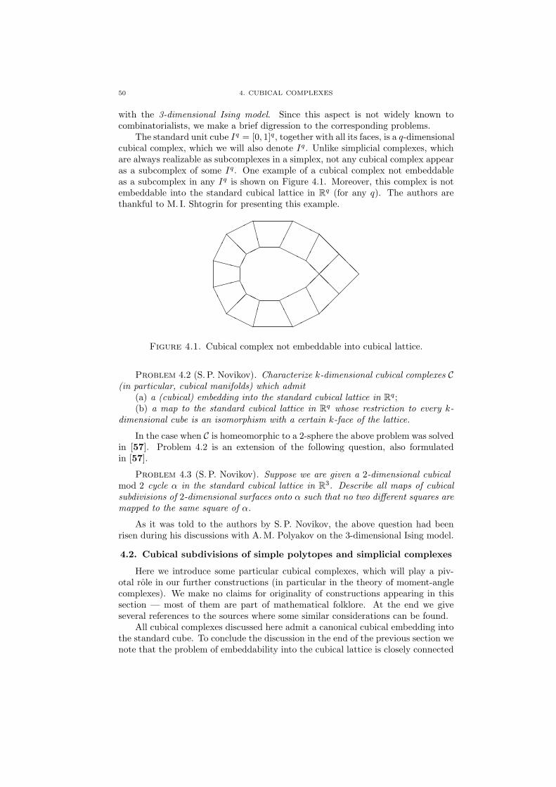
50 4. CUBICAL COMPLEXES
with the 3-dimensional Ising model. Since this aspect is not widely known tocombinatorialists, we make a brief digression to the corresponding problems.
The standard unit cube Iq = [0, 1]q, together with all its faces, is a q-dimensionalcubical complex, which we will also denote Iq. Unlike simplicial complexes, whichare always realizable as subcomplexes in a simplex, not any cubical complex appearas a subcomplex of some Iq. One example of a cubical complex not embeddableas a subcomplex in any Iq is shown on Figure 4.1. Moreover, this complex is notembeddable into the standard cubical lattice in Rq (for any q). The authors arethankful to M. I. Shtogrin for presenting this example.
¢¢¢©©© HHH
@@
@
@@
@@@¡
¡¡
¡¡©©©HHHAA
A
¢¢©© HHH
@@¡¡©©©HH
AA
XXX
@@@
CCC
¢¢
¢ ¢¢
¢ ¡¡¡
@@@
AA
A
AA
A
¤¤¤¡
¡¡
»»»
Figure 4.1. Cubical complex not embeddable into cubical lattice.
Problem 4.2 (S. P. Novikov). Characterize k-dimensional cubical complexes C(in particular, cubical manifolds) which admit
(a) a (cubical) embedding into the standard cubical lattice in Rq;(b) a map to the standard cubical lattice in Rq whose restriction to every k-
dimensional cube is an isomorphism with a certain k-face of the lattice.
In the case when C is homeomorphic to a 2-sphere the above problem was solvedin [57]. Problem 4.2 is an extension of the following question, also formulatedin [57].
Problem 4.3 (S. P. Novikov). Suppose we are given a 2-dimensional cubicalmod 2 cycle α in the standard cubical lattice in R3. Describe all maps of cubicalsubdivisions of 2-dimensional surfaces onto α such that no two different squares aremapped to the same square of α.
As it was told to the authors by S. P. Novikov, the above question had beenrisen during his discussions with A. M. Polyakov on the 3-dimensional Ising model.
4.2. Cubical subdivisions of simple polytopes and simplicial complexes
Here we introduce some particular cubical complexes, which will play a piv-otal role in our further constructions (in particular in the theory of moment-anglecomplexes). We make no claims for originality of constructions appearing in thissection — most of them are part of mathematical folklore. At the end we giveseveral references to the sources where some similar considerations can be found.
All cubical complexes discussed here admit a canonical cubical embedding intothe standard cube. To conclude the discussion in the end of the previous section wenote that the problem of embeddability into the cubical lattice is closely connected
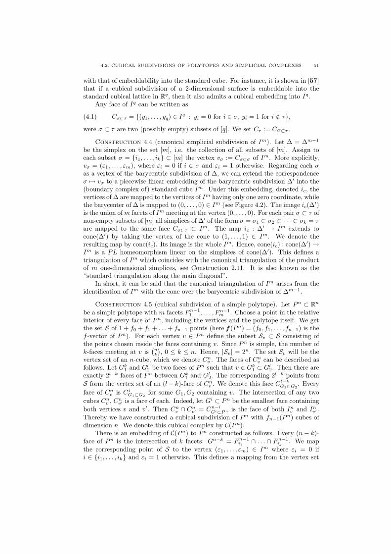
4.2. CUBICAL SUBDIVISIONS OF POLYTOPES AND SIMPLICIAL COMPLEXES 51
with that of embeddability into the standard cube. For instance, it is shown in [57]that if a cubical subdivision of a 2-dimensional surface is embeddable into thestandard cubical lattice in Rq, then it also admits a cubical embedding into Iq.
Any face of Iq can be written as
(4.1) Cσ⊂τ = (y1, . . . , yq) ∈ Iq : yi = 0 for i ∈ σ, yi = 1 for i /∈ τ,were σ ⊂ τ are two (possibly empty) subsets of [q]. We set Cτ := C∅⊂τ .
Construction 4.4 (canonical simplicial subdivision of Im). Let ∆ = ∆m−1
be the simplex on the set [m], i.e. the collection of all subsets of [m]. Assign toeach subset σ = i1, . . . , ik ⊂ [m] the vertex vσ := Cσ⊂σ of Im. More explicitly,vσ = (ε1, . . . , εm), where εi = 0 if i ∈ σ and εi = 1 otherwise. Regarding each σas a vertex of the barycentric subdivision of ∆, we can extend the correspondenceσ 7→ vσ to a piecewise linear embedding of the barycentric subdivision ∆′ into the(boundary complex of) standard cube Im. Under this embedding, denoted ic, thevertices of ∆ are mapped to the vertices of Im having only one zero coordinate, whilethe barycenter of ∆ is mapped to (0, . . . , 0) ∈ Im (see Figure 4.2). The image ic(∆′)is the union of m facets of Im meeting at the vertex (0, . . . , 0). For each pair σ ⊂ τ ofnon-empty subsets of [m] all simplices of ∆′ of the form σ = σ1 ⊂ σ2 ⊂ · · · ⊂ σk = τare mapped to the same face Cσ⊂τ ⊂ Im. The map ic : ∆′ → Im extends tocone(∆′) by taking the vertex of the cone to (1, . . . , 1) ∈ Im. We denote theresulting map by cone(ic). Its image is the whole Im. Hence, cone(ic) : cone(∆′) →Im is a PL homeomorphism linear on the simplices of cone(∆′). This defines atriangulation of Im which coincides with the canonical triangulation of the productof m one-dimensional simplices, see Construction 2.11. It is also known as the“standard triangulation along the main diagonal”.
In short, it can be said that the canonical triangulation of Im arises from theidentification of Im with the cone over the barycentric subdivision of ∆m−1.
Construction 4.5 (cubical subdivision of a simple polytope). Let Pn ⊂ Rn
be a simple polytope with m facets Fn−11 , . . . , Fn−1
m . Choose a point in the relativeinterior of every face of Pn, including the vertices and the polytope itself. We getthe set S of 1 + f0 + f1 + . . . + fn−1 points (here f (Pn) = (f0, f1, . . . , fn−1) is thef -vector of Pn). For each vertex v ∈ Pn define the subset Sv ⊂ S consisting ofthe points chosen inside the faces containing v. Since Pn is simple, the number ofk-faces meeting at v is
(nk
), 0 ≤ k ≤ n. Hence, |Sv| = 2n. The set Sv will be the
vertex set of an n-cube, which we denote Cnv . The faces of Cn
v can be described asfollows. Let Gk
1 and Gl2 be two faces of Pn such that v ∈ Gk
1 ⊂ Gl2. Then there are
exactly 2l−k faces of Pn between Gk1 and Gl
2. The corresponding 2l−k points fromS form the vertex set of an (l− k)-face of Cn
v . We denote this face Cl−kG1⊂G2
. Everyface of Cn
v is CiG1⊂G2
for some G1, G2 containing v. The intersection of any twocubes Cn
v , Cnv′ is a face of each. Indeed, let Gi ⊂ Pn be the smallest face containing
both vertices v and v′. Then Cnv ∩ Cn
v′ = Cn−iGi⊂P n is the face of both In
v and Inv′ .
Thereby we have constructed a cubical subdivision of Pn with fn−1(Pn) cubes ofdimension n. We denote this cubical complex by C(Pn).
There is an embedding of C(Pn) to Im constructed as follows. Every (n− k)-face of Pn is the intersection of k facets: Gn−k = Fn−1
i1∩ . . . ∩ Fn−1
ik. We map
the corresponding point of S to the vertex (ε1, . . . , εm) ∈ Im where εi = 0 ifi ∈ i1, . . . , ik and εi = 1 otherwise. This defines a mapping from the vertex set
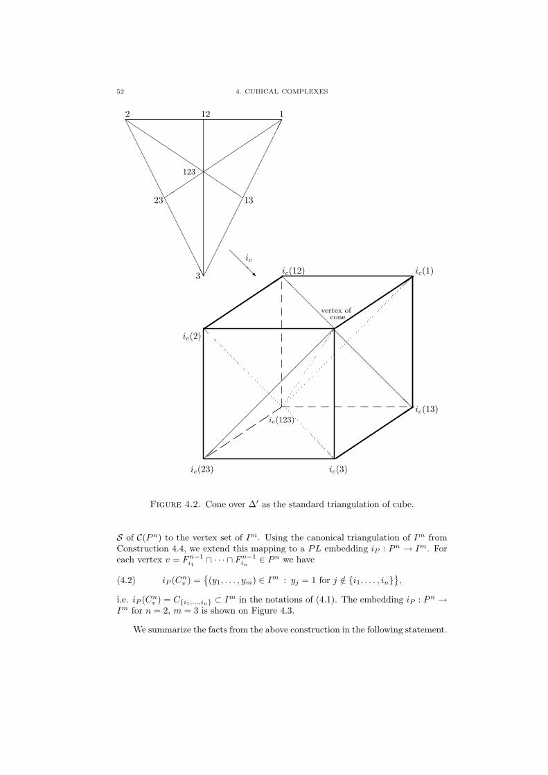
52 4. CUBICAL COMPLEXES
´´
´´
´´
´´
´´
´´
´´
´´
´´
´´
´´
´´
´´
´´
´´
´´
´´
´´
´´
´´
´´
´´
´´
´´
´´
´´
´´
´´
´´
´´
´´
´´
´´
´´
´´
´´
´´
´´
´´
´´
´´
´´
´´
´´
´´
´´
´´
´´
´´
´´
´´
´´
´´
´´
´´
´´
´´
´´
´´
´´
´´
´´
´´
´´
´´
´´
´´
´´
´´
´´
´´
´´
´´
´´
´´
´´
´´
´´
´´
´´
´´
´´
´´
´´
´´
´´
´´
¡¡
¡¡
¡¡
¡¡
¡¡
¡¡
¡¡¡
@@
@@
@@
@@
@@
@@
@@@
vertex ofcone
ic(1)
ic(2)
ic(3)ic(23)
ic(13)
ic(12)
ic(123)
AAAAAAAAAAAAAAAAAA
QQQ
¢¢¢¢¢¢¢¢¢¢¢¢¢¢¢¢¢¢´
´´
´´
´´
´´
´´
12
3
12
23 13
123
@@
@R
ic
Figure 4.2. Cone over ∆′ as the standard triangulation of cube.
S of C(Pn) to the vertex set of Im. Using the canonical triangulation of Im fromConstruction 4.4, we extend this mapping to a PL embedding iP : Pn → Im. Foreach vertex v = Fn−1
i1∩ · · · ∩ Fn−1
in∈ Pn we have
(4.2) iP (Cnv ) =
(y1, . . . , ym) ∈ Im : yj = 1 for j /∈ i1, . . . , in
,
i.e. iP (Cnv ) = Ci1,...,in ⊂ Im in the notations of (4.1). The embedding iP : Pn →
Im for n = 2, m = 3 is shown on Figure 4.3.
We summarize the facts from the above construction in the following statement.
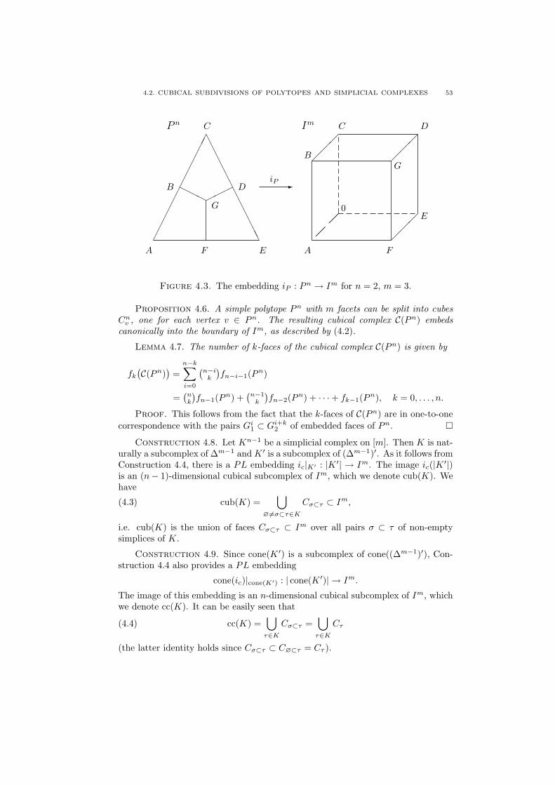
4.2. CUBICAL SUBDIVISIONS OF POLYTOPES AND SIMPLICIAL COMPLEXES 53
¢¢¢¢¢¢¢¢¢¢¢¢A
AAAAAAAAAAA
HHH©©©
-
¡¡
¡
¡¡
¡
¡¡
¡¡¡¡¡
0
A F E
G
B D
CP n
iP
A F
BG
C D
E
Im
Figure 4.3. The embedding iP : Pn → Im for n = 2, m = 3.
Proposition 4.6. A simple polytope Pn with m facets can be split into cubesCn
v , one for each vertex v ∈ Pn. The resulting cubical complex C(Pn) embedscanonically into the boundary of Im, as described by (4.2).
Lemma 4.7. The number of k-faces of the cubical complex C(Pn) is given by
fk
(C(Pn))
=n−k∑
i=0
(n−i
k
)fn−i−1(Pn)
=(nk
)fn−1(Pn) +
(n−1
k
)fn−2(Pn) + · · ·+ fk−1(Pn), k = 0, . . . , n.
Proof. This follows from the fact that the k-faces of C(Pn) are in one-to-onecorrespondence with the pairs Gi
1 ⊂ Gi+k2 of embedded faces of Pn. ¤
Construction 4.8. Let Kn−1 be a simplicial complex on [m]. Then K is nat-urally a subcomplex of ∆m−1 and K ′ is a subcomplex of (∆m−1)′. As it follows fromConstruction 4.4, there is a PL embedding ic|K′ : |K ′| → Im. The image ic(|K ′|)is an (n− 1)-dimensional cubical subcomplex of Im, which we denote cub(K). Wehave
(4.3) cub(K) =⋃
∅ 6=σ⊂τ∈K
Cσ⊂τ ⊂ Im,
i.e. cub(K) is the union of faces Cσ⊂τ ⊂ Im over all pairs σ ⊂ τ of non-emptysimplices of K.
Construction 4.9. Since cone(K ′) is a subcomplex of cone((∆m−1)′), Con-struction 4.4 also provides a PL embedding
cone(ic)|cone(K′) : | cone(K ′)| → Im.
The image of this embedding is an n-dimensional cubical subcomplex of Im, whichwe denote cc(K). It can be easily seen that
(4.4) cc(K) =⋃
τ∈K
Cσ⊂τ =⋃
τ∈K
Cτ
(the latter identity holds since Cσ⊂τ ⊂ C∅⊂τ = Cτ ).
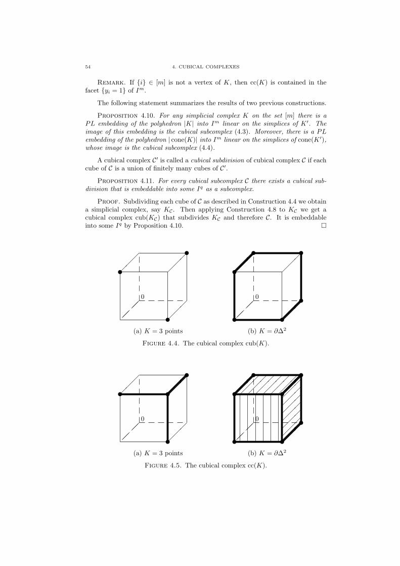
54 4. CUBICAL COMPLEXES
Remark. If i ∈ [m] is not a vertex of K, then cc(K) is contained in thefacet yi = 1 of Im.
The following statement summarizes the results of two previous constructions.
Proposition 4.10. For any simplicial complex K on the set [m] there is aPL embedding of the polyhedron |K| into Im linear on the simplices of K ′. Theimage of this embedding is the cubical subcomplex (4.3). Moreover, there is a PLembedding of the polyhedron | cone(K)| into Im linear on the simplices of cone(K ′),whose image is the cubical subcomplex (4.4).
A cubical complex C′ is called a cubical subdivision of cubical complex C if eachcube of C is a union of finitely many cubes of C′.
Proposition 4.11. For every cubical subcomplex C there exists a cubical sub-division that is embeddable into some Iq as a subcomplex.
Proof. Subdividing each cube of C as described in Construction 4.4 we obtaina simplicial complex, say KC . Then applying Construction 4.8 to KC we get acubical complex cub(KC) that subdivides KC and therefore C. It is embeddableinto some Iq by Proposition 4.10. ¤
¡¡
¡
¡¡
¡
u
u
u
¡¡
¡
¡¡¡¡
0
(a) K = 3 points
¡¡
¡
¡¡
¡
u
u
u
u
u
u
¡¡
¡
¡¡
¡
¡¡
¡
¡¡
¡
¡¡
¡
¡¡
¡
¡¡
¡
¡¡
¡
¡¡
¡
¡¡
¡
¡¡
¡
¡¡
¡
¡¡
¡
¡¡
¡
¡¡
¡
¡¡
¡
¡¡
¡
¡¡
¡
¡¡
¡
¡¡
¡
¡¡
¡
¡¡
¡
¡¡
¡
¡¡
¡
¡¡
¡
¡¡
¡
¡¡
¡
¡¡
¡
¡¡
¡
¡¡
¡
¡¡
¡
¡¡
¡
¡¡
¡¡¡¡¡
0
(b) K = ∂∆2
Figure 4.4. The cubical complex cub(K).
¡¡
¡
¡¡
¡
u
uu
u
¡¡
¡
¡¡
¡
¡¡
¡
¡¡
¡
¡¡
¡
¡¡
¡
¡¡
¡
¡¡
¡
¡¡
¡
¡¡
¡
¡¡
¡
¡¡
¡
¡¡
¡
¡¡
¡
¡¡
¡
¡¡
¡
¡¡¡¡
0
(a) K = 3 points
¡¡
¡
¡¡
¡
u
u
uu
u
u
u
¡¡
¡
¡¡
¡
¡¡
¡
¡¡
¡
¡¡
¡
¡¡
¡
¡¡
¡
¡¡
¡
¡¡
¡
¡¡
¡
¡¡
¡
¡¡
¡
¡¡
¡
¡¡
¡
¡¡
¡
¡¡
¡
¡¡
¡
¡¡
¡
¡¡
¡
¡¡
¡
¡¡
¡
¡¡
¡
¡¡
¡
¡¡
¡
¡¡
¡
¡¡
¡
¡¡
¡
¡¡
¡
¡¡
¡
¡¡
¡
¡¡
¡
¡¡
¡
¡¡
¡
¡¡
¡
¡¡
¡
¡¡
¡
¡¡
¡
¡¡
¡
¡¡
¡
¡¡
¡
¡¡
¡
¡¡
¡
¡¡
¡
¡¡
¡
¡¡
¡
¡¡
¡
¡¡
¡
¡¡
¡¡¡¡¡
¡¡
¡
¡¡
¡
¡¡
¡
¡¡
¡
¡¡
¡
¡¡
¡
¡¡
¡¡
¡¡
¡¡
¡¡
¡¡
¡¡
¡¡
¡¡
0
(b) K = ∂∆2
Figure 4.5. The cubical complex cc(K).
4.2. CUBICAL SUBDIVISIONS OF POLYTOPES AND SIMPLICIAL COMPLEXES 55
Example 4.12. The cubical complex cub(K) in the case when K is a disjointunion of 3 vertices is shown on Figure 4.4 (a). Figure 4.4 (b) shows that for thecase K = ∂∆2, the boundary complex of a 2-simplex. The corresponding cubicalcomplexes cc(K) are indicated on Figure 4.5 (a) and (b).
Remark. As a topological space, cub(K) is homeomorphic to |K|, while cc(K)is homeomorphic to | cone(K)|. On the other hand, there is the cubical complexcub(cone(K)), also homeomorphic to | cone(K)|. However, as cubical complexes,cc(K) and cub(cone(K)) differ (since cone(K ′) 6= (cone(K))′).
Let P be a simple n-polytope and KP the corresponding simplicial (n − 1)-sphere (the boundary of the polar simplicial polytope P ∗). Then cc(KP ) coincideswith the cubical complex C(P ) from Construction 4.5. More precisely, cc(KP ) =iP (C(P )). Thus, Construction 4.5 is a particular case of Construction 4.9 (compareFigures 4.2–4.5).
Remark. Different versions of Construction 4.9 can be found in [10] and insome earlier papers listed there on p. 299. In [48, p. 434] a similar construction wasintroduced while studying certain toric spaces; we will return to this in the nextchapters. A version of the cubical subcomplex cub(K) ⊂ Im appeared in [120] inconnection with Problem 4.2.

CHAPTER 5
Toric and quasitoric manifolds
5.1. Toric varieties
Toric varieties appeared in algebraic geometry in the beginning of 1970s in con-nection with compactification problems for algebraic torus actions. The geometry oftoric varieties very quickly has become one of the most fascinating topics in algebraicgeometry and found applications in many mathematical sciences, which otherwiseseemed far from each other. We have already mentioned the proof for the “only if”part of the g-theorem for simplicial polytopes given by Stanley. Other remarkableapplications include counting lattice points and volumes of lattice polytopes; rela-tions with Newton polytopes and singularities (after Khovanskii and Kushnirenko);discriminants, resultants and hypergeometric functions (after Gelfand, Kapranovand Zelevinsky); reflexive polytopes and mirror symmetry for Calabi–Yau toric hy-persurfaces (after Batyrev). Standard references in the toric geometry are Danilov’ssurvey [46] and books by Oda [105], Fulton [64] and Ewald [61]. More recent sur-vey article by Cox [45] covers new applications, including mentioned above. We arenot going to give another review of the toric geometry here. Instead, in this sectionwe stress upon some topological and combinatorial aspects of toric varieties. Wealso give Stanley’s argument for the g-theorem.
5.1.1. Toric varieties and fans. Let C∗ = C \ 0 denote the multiplicativegroup of complex numbers. The product (C∗)n of n copies of C∗ is known as thetorus in the theory of algebraic groups. In topology, the torus Tn is the productof n circles. We keep the topological notations, referring to (C∗)n as the algebraictorus. The torus Tn is a subgroup of the algebraic torus (C∗)n in the standardway:
(5.1) Tn =(
e2πiϕ1 , . . . , e2πiϕn) ∈ Cn
,
where (ϕ1, . . . , ϕn) is running through Rn.
Definition 5.1. A toric variety is a normal algebraic variety M containingthe algebraic torus (C∗)n as a Zariski open subset in such a way that the naturalaction of (C∗)n on itself extends to an action on M .
Hence, (C∗)n acts on M with a dense orbit.One of the most beautiful properties of toric varieties is that all of their subtlest
algebro-geometrical properties can be translated into the language of combinatoricsand convex geometry. The following definition introduces necessary combinatorialnotions.
Definition 5.2 (Fans terminology). Let Rn be the Euclidean space and Zn ⊂Rn the integral lattice. Given a finite set of vectors l1, . . . , ls ∈ Rn, define the
57
58 5. TORIC AND QUASITORIC MANIFOLDS
convex polyhedral cone σ spanned by l1, . . . , ls by
(5.2) σ = r1l1 + · · ·+ rsls ∈ Rn : ri ≥ 0.Any convex polyhedral cone is a convex polyhedron in the sense of Definition 1.2.Hence, the faces of a convex polyhedral cone are defined. A cone σ is rational ifits generator vectors l1, . . . , ls can be taken from Zn and is strongly convex if itcontains no line through the origin. All cones considered below are strongly convexand rational. A cone is simplicial (respectively, non-singular) if it is generated bya part of a basis of Rn (respectively, Zn). A fan is a set Σ of cones in Rn suchthat each face of a cone in Σ is also a cone in Σ, and the intersection of two conesin Σ is a face of each. A fan Σ in Rn is called complete if the union of all conesfrom Σ is Rn. A fan Σ is simplicial (respectively, non-singular) if all cones of Σare simplicial (respectively, non-singular). Let Σ be a simplicial fan in Rn withm one-dimensional cones (or rays). Choose generator vectors l1, . . . , lm for theserays to be integer and primitive, i.e. with relatively prime integer coordinates. Thefan Σ defines a simplicial complex KΣ on the vertex set [m], which is called theunderlying complex of Σ. By definition, i1, . . . , ik ⊂ [m] is a simplex of KΣ if andonly if l i1 , . . . , l ik
span a cone of Σ. Obviously, Σ is complete if and only if KΣ isa simplicial (n− 1)-sphere.
As it is explained in any of the above mentioned sources, there is a one-to-onecorrespondence between fans in Rn and toric varieties of complex dimension n.We will denote the toric variety corresponding to a fan Σ by MΣ. It follows that,in principle, all geometrical and topological properties of a toric variety can beretrieved from the combinatorics of the underlying fan.
The inclusion poset of (C∗)n-orbits of MΣ is isomorphic to the poset of facesof Σ with reversed inclusion. That is, the k-dimensional cones of Σ correspond tothe codimension-k orbits of the algebraic torus action on MΣ. In particular, then-dimensional cones correspond to the fixed points, while the origin correspondsto the unique dense orbit. The toric variety MΣ is compact if and only if Σ iscomplete. If Σ is simplicial then MΣ is an orbifold (i.e. is locally homeomorphic tothe quotient of R2n by a finite group action). Finally, MΣ is non-singular (smooth)if and only if Σ is non-singular, which explains the notation. Smooth toric varietiessometimes are called toric manifolds in the algebraic geometry literature.
Remark. Bistellar moves (see Definition 2.39) on the simplicial complex KΣ
can be interpreted as operations on the fan Σ. On the level of toric varieties, suchan operation corresponds to a flip (a blow-up followed by a subsequent blow-downalong different subvariety). This issue is connected with the question of factoriza-tion of a proper birational morphism between two complete smooth (or normal)algebraic varieties of dimension ≥ 3 into a sequence of blow-ups and blow-downswith smooth centers, a fundamental problem in the birational algebraic geometry.Two version of this problem are usually distinguished: the Strong factorizationconjecture, which asks if it is possible to represent a birational morphism by asequence of blow-ups followed by a sequence of blow-downs, and the Weak factor-ization conjecture, in which the order of blow-ups and blow-downs is insignificant.Since all toric varieties are rational, any two toric varieties of the same dimensionare birationally equivalent. Weak (equivariant) factorization conjecture for smoothcomplete toric varieties was proved by WÃlodarczyk [140] (announced in 1991) usinginterpretation of equivariant flips on toric varieties as bistellar move-type operations
5.1. TORIC VARIETIES 59
on the corresponding fans. Thereby the weak factorization theorem for smooth toricvarieties reduces to the statement that any two complete non-singular fans in Rn
can be taken one to another by a finite sequence of bistellar move-type operationsin which all intermediate fans are non-singular. This result is the essence of [140].(Note that the statement does not reduce to Pachner’s Theorem 2.40 because ofthe additional smoothness condition.) The equivariant toric strong factorizationconjecture was proved by Morelli [102].
5.1.2. Cohomology of non-singular toric varieties. Danilov–Jurkiewicztheorem allows to read the integer cohomology ring of a non-singular toric varietydirectly from the underlying fan Σ. Write the primitive integer vectors along therays of Σ in the standard basis of Zn:
l j = (l1j , . . . , lnj)t, j = 1, . . . ,m.
Assign to each vector l j the indeterminate vj of degree 2, and define linear forms
θi := li1v1 + · · ·+ limvm ∈ Z[v1, . . . , vm], 1 ≤ i ≤ n.
Denote by JΣ the ideal in Z[v1, . . . , vm] spanned by these linear forms, i.e. JΣ =(θ1, . . . , θn). The images of θ1, . . . , θn and JΣ in the Stanley–Reisner ring Z(KΣ) =Z[v1, . . . , vm]/IKΣ (see Definition 3.1) will be denoted by the same symbols.
Theorem 5.3 (Danilov and Jurkiewicz). Let Σ be a complete non-singular fanin Rn, and MΣ the corresponding toric variety. Then
(a) The Betti numbers (the ranks of homology groups) of MΣ vanish in odddimensions, while in even dimensions are given by
b2i(MΣ) = hi(KΣ), i = 0, 1, . . . , n,
where h(KΣ) = (h0, . . . , hn) is the h-vector of KΣ.(b) The cohomology ring of MΣ is given by
H∗(MΣ;Z) = Z[v1, . . . , vm]/(IKΣ + JΣ) = Z(KΣ)/JΣ,
where vi, 1 ≤ i ≤ m, denote the 2-dimensional cohomology classes dual to invari-ant divisors (codimension-two submanifolds) Di corresponding to the rays of Σ.Moreover, θ1, . . . , θn is a regular sequence in Z(KΣ).
This theorem was proved by Jurkiewicz [82] for projective smooth toric varietiesand by Danilov [46, Theorem 10.8] in the general case. Note that the ideal IKΣ isdetermined only by the combinatorics of the fan (i.e. by the intersection poset ofΣ), while JΣ depends on the geometry of Σ. One can observe that the first part ofTheorem 5.3 follows from the second part and Lemma 3.8.
Remark. As it was shown by Danilov, the Q-coefficient version of Theorem 5.3is also true for simplicial fans and toric varieties.
It follows from Theorem 5.3 that the cohomology of MΣ is generated by two-dimensional classes. This is the first thing to check if one wishes to determinewhether or not a given algebraic variety or smooth manifold arises as a non-singular(or simplicial) toric variety. Another interesting algebraic-geometrical property ofnon-singular toric varieties, suggested by Theorem 5.3, is that the Chow ring [64,§ 5.1] of MΣ coincides with its integer cohomology ring.
60 5. TORIC AND QUASITORIC MANIFOLDS
5.1.3. Toric varieties from polytopes.
Construction 5.4 (Normal fan and toric varieties from polytopes). Supposewe are given an n-polytope (1.1) with vertices in the integer lattice Zn ⊂ Rn.Such a polytope is called integral, or lattice. Then the vectors l i in (1.1), 1 ≤i ≤ m, can be chosen integer and primitive, and the numbers ai can be choseninteger. Note that l i is normal to the facet Fi ⊂ Pn and is pointing inside thepolytope P . Define the complete fan Σ(P ) whose cones are generated by thosesets of normal vectors l i1 , . . . , l ik
whose corresponding facets Fi1 , . . . , Fikhave non-
empty intersection in P . The fan Σ(P ) is called the normal fan of P . Alternatively,if 0 ∈ P then the normal fan consists of cones over the faces of the polar polytope P ∗.Define the toric variety MP := MΣ(P ). The variety MP is smooth if and only ifP is simple and the normal vectors l i1 , . . . , l in
of any set of n facets Fi1 , . . . , Fin
meeting at the same vertex form a basis of Zn.
Remark. Every combinatorial simple polytope is rational , that is, admits aconvex realization with rational vertex coordinates. Indeed, there is a small per-turbation of defining inequalities in (1.1) that makes all of them rational but doesnot change the combinatorial type (since the half-spaces defined by the inequal-ities are in general position). As a result, one gets a simple polytope P ′ of thesame combinatorial type with rational vertex coordinates. To obtain a realizationwith integral vertex coordinates we just take the magnified polytope kP ′ for ap-propriate k ∈ Z. We note that this is not the case in general: in every dimension≥ 5 there exist non-rational convex polytopes (non-simple and non-simplicial), seee.g. [145, Example 6.21] and discussion there. In dimension 3 all convex poly-topes are rational, and in dimension 4 the existence of non-rational polytopes is anopen problem. Returning to simple polytopes, we note that different realizations ofa given combinatorial simple polytope as lattice polytopes may produce different(even topologically) toric varieties MP . At the same time there exist combinatorialsimple polytopes that do not admit any lattice realization with smooth MP . Wepresent one such example in the next section, see Example 5.26.
The underlying topological space of a toric variety MP can be identified withthe quotient space Tn × Pn/∼ for some equivalence relation ∼ using the followingconstruction (see e.g. [64, § 4.1]).
Construction 5.5 (Toric variety as an identification space). We identify thetorus Tn (5.1) with the quotient Rn/Zn. For each point q ∈ Pn define G(q) as thesmallest face that contains q in its relative interior. The normal subspace to G(q),denoted N , is spanned by the primitive vectors l i (see (1.1)) corresponding to thosefacets Fi which contain G(q). (If Pn is simple then there are exactly codimG(q)such facets; in general there are more of them.) Since N is a rational subspace,it projects to a subtorus of Tn, which we denote T (q). Note that dim T (q) =n− dim G(q). Then, as a topological space,
MP = Tn × Pn/∼,
where (t1, p) ∼ (t2, q) if and only if p = q and t1t−12 ∈ T (q). The subtori T (q)
are the isotropy subgroups for the action of Tn on MP , and Pn is identified withthe orbit space. Note that if q is a vertex of Pn then T (q) = Tn, so the verticescorrespond to the Tn-fixed points of MP . At the other extreme, if q ∈ intPn
5.1. TORIC VARIETIES 61
then T (q) = e, so the Tn-action is free over the interior of the polytope. Moregenerally, if π : MP → Pn is the quotient projection then
π−1(intG(q)
)=
(Tn/T (q)
)× intG(q).
Remark. The above construction can be generalized to all complete toric va-rieties (not necessarily coming from polytopes) by replacing Pn by an n-ball withcellular decomposition on the boundary. This cellular decomposition is “dual” tothat defined by the complete fan.
Construction 5.4 allows to define the simplicial fan Σ(P ) and the toric varietyMP from any lattice simple polytope P . However, the lattice polytope P con-tains more geometrical information than the fan Σ(P ). Indeed, besides the normalvectors l i, which determine the fan, we also have numbers ai ∈ Z, 1 ≤ i ≤ m,(see (1.1)). In the notations of Theorem 5.3, it is well known in the toric geometrythat the linear combination D = a1D1 + · · · + amDm is an ample divisor on MP .It defines a projective embedding MP ⊂ CP r for some r (which can be taken to bethe number of vertices of P ). This implies that all toric varieties from polytopes areprojective. Conversely, given a smooth projective toric variety M ⊂ CP r, one getsvery ample divisor (line bundle) D of hyperplane section whose zero cohomology isgenerated by the sections corresponding to lattice points in a certain lattice simplepolytope P . For this P one has M = MP . Let ω := a1v1+· · ·+amvm ∈ H2(MP ;Q)be the cohomology class of D.
Theorem 5.6 (Hard Lefschetz theorem for toric varieties). Let Pn be a latticesimple polytope (1.1), MP the toric variety defined by P , and ω = a1v1 + · · · +amvm ∈ H2(MP ;Q) the above defined cohomology class. Then the maps
Hn−i(MP ;Q) · ωi
−−−−→ Hn+i(MP ;Q), 1 ≤ i ≤ n,
are isomorphisms.
It follows from the projectivity that if MP is smooth then it is Kahler, and ω is theclass of the Kahler 2-form.
Remark. As it is stated, Theorem 5.6 applies only to simplicial projectivetoric varieties. However it remains true for any projective toric variety if we replacethe ordinary cohomology by the (middle perversity) intersection cohomology . Formore details see the discussion in [64, § 5.2].
Example 5.7. The complex projective space CPn = (z0 : z1 : · · · : zn), zi ∈C is a toric variety. The algebraic torus (C∗)n acts on CPn by
(t1, . . . , tn) · (z0 : z1 : · · · : zn) = (z0 : t1z1 : · · · : tnzn).
Obviously, (C∗)n ⊂ Cn ⊂ CPn is a dense open subset. A sample fan definingCPn consists of the cones spanned by all proper subsets of the set of (n + 1)vectors e1, . . . , en,−e1−· · ·−en in Rn. Theorem 5.3 identifies the cohomology ringH∗(CPn;Z) = Z[u]/(un+1), dim u = 2, with the quotient ring
Z[v1, . . . , vn+1]/(v1 · · · vn+1, v1 − vn+1, . . . , vn − vn+1).
The toric variety CPn arises from a polytope: CPn = MP , where P is the standardn-simplex (1.2). The corresponding class ω ∈ H2(CPn;Q) from Theorem 5.6 isrepresented by vn+1.

62 5. TORIC AND QUASITORIC MANIFOLDS
Now we are ready to give Stanley’s argument for the “only if” part of theg-theorem for simple polytopes.
Proof of the necessity part of Theorem 1.29. Realize the simple poly-tope as a lattice polytope Pn ⊂ Rn. Let MP be the corresponding toric vari-ety. Part (a) is already proved (Theorem 1.20). It follows from Theorem 5.6that the multiplication by ω ∈ H2(MP ;Q) is a monomorphism H2i−2(MP ;Q) →H2i(MP ;Q) for i ≤ [
n2
]. This together with part (a) of Theorem 5.3 gives hi−1 ≤ hi,
0 ≤ i ≤ [n2
], thus proving (b). To prove (c), define the graded commutative Q-
algebra A := H∗(MP ;Q)/(ω). Then A0 = Q, A2i = H2i(MP ;Q)/ω ·H2i−2(MP ;Q)for 1 ≤ i ≤ [
n2
], and A is generated by degree-two elements (since so is H∗(MP ;Q)).
It follows from Theorem 1.32 that the numbers dim A2i = hi − hi−1, 0 ≤ i ≤ [n2
],
are the components of an M -vector, thus proving (c) and the whole theorem. ¤
Remark. The Dehn–Sommerville equations now can be interpreted as thePoincare duality for MP . Even though MP needs not to be smooth, the rationalcohomology algebra of a simplicial toric variety (or toric orbifold) still satisfies thePoincare duality.
The Hard Lefschetz theorem (Theorem 5.6) holds only for projective toric vari-eties. This implies that Stanley’s argument can not be directly generalized beyondthe polytopal sphere case. So far this case is the only generality in which meth-ods involving the Hard Lefschetz theorem are efficient for proving the g-theorem(see also the discussion at the end of section 7.6). However, the cohomology oftoric varieties has been shown to be quite helpful in generalizing statements likethe g-theorem in a different direction, namely, to the case of general (not neces-sarily simple or simplicial) convex polytopes. So suppose Pn is a convex latticen-polytope. It gives rise, as described in Construction 5.4, to a projective toricvariety MP . If Pn is not simple then MP has worse than just orbifold singular-ities and its ordinary cohomology behaves badly. The Betti numbers of MP arenot determined by the combinatorial type of Pn and do not satisfy the Poincareduality. On the other hand, it turns out that the dimensions hi of the intersectioncohomology of MP are combinatorial invariants of Pn. The vector
h(Pn) = (h0, h1, . . . , hn)
is called the intersection h-vector of Pn. If Pn is simple, then the intersectionh-vector coincides with the ordinary one, but in general h(Pn) is not determinedby the face vector of Pn and its combinatorial definition is quite subtle, see [126]for details. The intersection h-vector satisfies the “Dehn–Sommerville equations”hi = hn−i, and the Hard Lefschetz theorem shows that it also satisfies the GLBCinequalities:
h0 ≤ h1 ≤ · · · ≤ h[n2
].
In the case when Pn can not be realized as a lattice polytope (that is, Pn isnon-rational, see the remark after Construction 5.4) the combinatorial definition ofintersection h-vector still works, but it is not known whether the above inequalitiescontinue to hold. Some progress in this direction has been achieved in [27], [134].
To summarise, we may say that although Hard Lefschetz and intersection co-homology methods so far are not very helpful in the non-convex situation (like PL
5.2. QUASITORIC MANIFOLDS 63
or simplicial spheres), they still are quite powerful in the case of general convexpolytopes.
Now we look more closely at the action of the torus Tn ⊂ (C∗)n on a non-singular compact toric variety M . This action is “locally equivalent” to the standardaction of Tn on Cn, see the next section for the precise definition. The orbit spaceM/Tn is homeomorphic to an n-ball, invested with the topological structure ofmanifold with corners by the fixed point sets of appropriate subtori, see [64, § 4.1].Roughly speaking, a manifold with corners is a space that is locally modelled byopen subsets of the positive cone Rn
+ (1.4). From this description it is easy todeduce the strict definition [80], which we omit here.
Construction 5.8. Let Pn be a simple polytope. For any vertex v ∈ Pn
denote by Uv the open subset of Pn obtained by deleting all faces not containing v.Obviously, Uv is diffeomorphic to Rn
+ (and even affinely isomorphic to an open setof Rn
+ containing 0). It follows that Pn is a manifold with corners, with atlas Uv.As suggested by Construction 5.5, if smooth M arises from a lattice poly-
tope Pn (which is therefore simple) then the orbit space M/Tn is diffeomorphic, asa manifold with corners, to Pn. Furthermore, in this case there exists an explicitmap M → Rn (the moment map) with image Pn ⊂ Rn and Tn-orbits as fibres,see [64, §4.2]. (We will return to moment maps and some aspects of symplecticgeometry in section 8.2.) The identification space description of a non-singularprojective toric variety (Construction 5.5) motivated Davis and Januszkiewicz [48]to introduce a topological counterpart of the toric geometry, namely, the study ofquasitoric manifolds. We proceed with their description in the next section.
5.2. Quasitoric manifolds
Quasitoric manifolds can be viewed as a “topological approximation” to alge-braic non-singular projective toric varieties. This notion appeared in [48] underthe name “toric manifolds”. We use the term “quasitoric manifold”, since “toricmanifold” is reserved in the algebraic geometry for “non-singular toric variety”.In the consequent definitions we follow [48], taking into account adjustments andspecifications from [38]. Like in the case of toric varieties, we first give a definitionof a quasitoric manifold from the general topological point of view (as a manifoldwith a certain nice torus action), and then specify a combinatorial construction(similar to the construction of toric varieties from fans or polytopes).
5.2.1. Quasitoric manifolds and characteristic maps. As in the previoussection, we regard the torus Tn as the standard subgroup (5.1) in (C∗)n, therebyspecifying the orientation and the coordinate subgroups Ti
∼= S1 (i = 1, . . . , n)in Tn. We refer to the representation of Tn by diagonal matrices in U(n) as thestandard action on Cn. The orbit space of this action is the positive cone Rn
+ (1.4).The canonical projection
Tn × Rn+ → Cn : (t1, . . . , tn)× (x1, . . . , xn) → (t1x1, . . . , tnxn)
identifies Cn with a quotient space Tn × Rn+/∼. This quotient will serve as the
“local model” for some other identification spaces below.Let M2n be a 2n-dimensional manifold with an action of the torus Tn (a Tn-
manifold for short).
64 5. TORIC AND QUASITORIC MANIFOLDS
Definition 5.9. A standard chart on M2n is a triple (U, f, ψ), where U is aTn-stable open subset of M2n, ψ is an automorphism of Tn, and f is a ψ-equivarianthomeomorphism f : U → W with some (Tn-stable) open subset W ⊂ Cn. (Thelatter means that f(t · y) = ψ(t)f(y) for all t ∈ Tn, y ∈ U .) Say that a Tn-actionon M2n is locally standard if M2n has a standard atlas, that is, every point of M2n
lies in a standard chart.
The orbit space for a locally standard action of Tn on M2n is an n-dimensionalmanifold with corners. Quasitoric manifolds correspond to the case when this orbitspace is diffeomorphic, as manifold with corners, to a simple polytope Pn. Notethat two simple polytopes are diffeomorphic as manifolds with corners if and onlyif they are combinatorially equivalent.
Definition 5.10. Given a combinatorial simple polytope Pn, a Tn-manifoldM2n is called a quasitoric manifold over Pn if the following two conditions aresatisfied:
(a) the Tn-action is locally standard;(b) there is a projection map π : M2n → Pn constant on Tn-orbits which
maps every k-dimensional orbit to a point in the interior of a codimension-k face of Pn, k = 0, . . . , n.
It follows that the Tn-action on a quasitoric manifold M2n is free over the interiorof the quotient polytope Pn, while the vertices of Pn correspond to the Tn-fixedpoints of M2n. Direct comparison with Construction 5.5 suggests that every smooth(projective) toric variety MP coming from a simple lattice polytope Pn is a qua-sitoric manifold over the corresponding combinatorial polytope. We will return tothis below in Example 5.19.
Suppose Pn has m facets F1, . . . , Fm. By the definition, for every facet Fi,the pre-image π−1(int Fi) consists of codimension-one orbits with the same 1-dimensional isotropy subgroup, which we denote T (Fi). It can be easily seen thatπ−1(Fi) is an 2(n − 1)-dimensional quasitoric (sub)manifold over Fi, with respectto the action of Tn/T (Fi). We denote it M
2(n−1)i and refer to it as the facial
submanifold corresponding to Fi. Its isotropy subgroup T (Fi) can be written as
(5.3) T (Fi) =(
e2πiλ1iϕ, . . . , e2πiλniϕ) ∈ Tn
,
where ϕ ∈ R and λλi = (λ1i, . . . , λni)t ∈ Zn is a primitive vector. This λλi isdetermined by T (Fi) only up to a sign. A choice of sign specifies an orientationfor T (Fi). For now we do not care about this sign and choose it arbitrary. Moredetailed treatment of signs and orientations is the subject of the next section. Werefer to λλi as the facet vector corresponding to Fi. The correspondence
(5.4) ` : Fi 7→ T (Fi)
is called the characteristic map of M2n.Suppose we have a codimension-k face Gn−k, written as an intersection of k
facets: Gn−k = Fi1 ∩ · · · ∩ Fik. Then the submanifolds Mi1 , . . . ,Mik
intersecttransversally in a submanifold M(G)2(n−k), which we refer to as the facial sub-manifold corresponding to G. The map T (Fi1) × · · · × T (Fik
) → Tn is injectivesince T (Fi1) × · · · × T (Fik
) is identified with the k-dimensional isotropy subgroupof M(G)2(n−k). It follows that the vectors λλi1 , . . . , λλik
form a part of integral basisof Zn.
5.2. QUASITORIC MANIFOLDS 65
Let Λ be integer (n×m)-matrix whose i-th column is formed by the coordinatesof the facet vector λλi, i = 1, . . . , m. Every vertex v ∈ Pn is an intersection of nfacets: v = Fi1 ∩· · ·∩Fin
. Let Λ(v) := Λ(i1,...,in) be the maximal minor of Λ formedby the columns i1, . . . , in. Then
(5.5) det Λ(v) = ±1.
The correspondence
Gn−k 7→ isotropy subgroup of M(G)2(n−k)
extends the characteristic map (5.4) to a map from the face poset of Pn to theposet of subtori of Tn.
Definition 5.11. Let Pn be a combinatorial simple polytope and ` is a mapfrom facets of Pn to one-dimensional subgroups of Tn. Then (Pn, `) is called acharacteristic pair if `(Fi1)×· · ·×`(Fik
) → Tn is injective whenever Fi1∩· · ·∩Fik6=
∅.
The map ` directly extends to a map from the face poset of Pn to the poset ofsubtori of Tn, so we have subgroup `(G) ⊂ Tn for every face G of Pn.
Like in the case of standard action of Tn on Cn, there is a projection Tn×Pn →M2n whose fibre over x ∈ M2n is the isotropy subgroup of x. This argument can beused for reconstructing the quasitoric manifold from any given characteristic pair(Pn, `).
Construction 5.12 (Quasitoric manifold from characteristic pair). Given apoint q ∈ Pn, we denoted by G(q) the minimal face containing q in its relativeinterior. Now set
M2n(`) := (Tn × Pn)/∼,
where (t1, p) ∼ (t2, q) if and only if p = q and t1t−12 ∈ `(G(q)) (compare with
Construction 5.5 for toric varieties). The free action of Tn on Tn × Pn obviouslydescends to an action on (Tn ×Pn)/∼, with quotient Pn. The latter action is freeover the interior of Pn and has a fixed point for each vertex of Pn. Just as Pn iscovered by the open sets Uv, based on the vertices and diffeomorphic to Rn
+ (seeConstruction 5.8), so the space (Tn × Pn)/∼ is covered by open sets (Tn ×Uv)/∼homeomorphic to (Tn × Rn
+)/∼, and therefore to Cn. This implies that the Tn-action on (Tn×Pn)/∼ is locally standard, and therefore (Tn×Pn)/∼ is a quasitoricmanifold.
Definition 5.13. Given an automorphism ψ : Tn → Tn, say that two qua-sitoric manifolds M2n
1 , M2n2 over the same Pn are ψ-equivariantly diffeomorphic
if there is a diffeomorphism f : M2n1 → M2n
2 such that f(t · x) = ψ(t)f(x) forall t ∈ Tn, x ∈ M2n
1 . The automorphism ψ induces an automorphism ψ∗ of theposet of subtori of Tn. Any such automorphism descends to a ψ-translation ofcharacteristic pairs, in which the two characteristic maps differ by ψ∗.
The following proposition is proved as Proposition 1.8 in [48] (see also [38,Proposition 2.6]).
Proposition 5.14. Construction 5.12 defines a bijection between ψ-equivariantdiffeomorphism classes of quasitoric manifolds and ψ-translations of pairs (Pn, `).
When ψ is the identity, we deduce that two quasitoric manifolds are equivari-antly diffeomorphic if and only if their characteristic maps are the same.

66 5. TORIC AND QUASITORIC MANIFOLDS
5.2.2. Cohomology of quasitoric manifolds. The cohomology ring struc-ture of a quasitoric manifold is similar to that of a non-singular toric variety. To seethis analogy we first describe a cell decomposition of M2n with even dimensionalcells (a perfect cellular structure) and calculate the Betti numbers accordingly,following [48].
Construction 5.15. We recall the “Morse-theoretical arguments” from theproof of Dehn–Sommerville relations (Theorem 1.20). There we turned the 1-skeleton of Pn into a directed graph and defined the index ind(v) of a vertex v ∈ Pn
as the number of incident edges that point towards v. These inward edges span aface Gv of dimension ind(v). Denote by Gv the subset of Gv obtained by deleting allfaces not containing v. Obviously, Gv is diffeomorphic to Rind(v)
+ and is contained inthe open set Uv ⊂ Pn from Construction 5.8. Then ev := π−1Gv is identified withCind(v), and the union of the ev over all vertices of Pn define a cellular decomposi-tion of M2n. Note that all cells are even-dimensional and the closure of the cell ev
is the facial submanifold M(Gv)2 ind(v) ⊂ M2n. This argument was earlier used byKhovanskii [84] for constructing perfect cellular decompositions of toric varieties.
Proposition 5.16. The Betti numbers of M2n vanish in odd dimensions, whilein even dimensions are given by
b2i(M2n) = hi(Pn), i = 0, 1, . . . , n,
where h(Pn) = (h0, . . . , hn) is the h-vector of Pn.
Proof. The 2i-th Betti number equals the number of 2i-dimensional cells inthe cellular decomposition constructed above. This number equals the number ofvertices of index i, which is hi(Pn) by the argument from the proof of Theorem 1.20.
¤
Given a quasitoric manifold M2n with characteristic map (5.4) and facet vectorsλλi = (λ1i, . . . , λni)t ∈ Zn, i = 1, . . . , m, define linear forms
(5.6) θi := λi1v1 + · · ·+ λimvm ∈ Z[v1, . . . , vm], 1 ≤ i ≤ n.
The images of these linear forms in the Stanley–Reisner ring Z(Pn) will be denotedby the same letters.
Lemma 5.17 (Davis and Januszkiewicz). θ1, . . . , θn is a (degree-two) regularsequence in Z(Pn).
Let J` denote the ideal in Z(Pn) generated by θ1, . . . , θn.
Theorem 5.18 (Davis and Januszkiewicz). The cohomology ring of M2n isgiven by
H∗(M2n;Z) = Z[v1, . . . , vm]/(IP + J`) = Z(Pn)/J`,
where vi is the 2-dimensional cohomology class dual to the facial submanifoldM
2(n−1)i (with arbitrary orientation chosen), i = 1, . . . , m.
We give proofs for the above two statements in section 6.5.
Remark. Change of sign of vector λλi corresponds to passing from vi to −vi
in the description of the cohomology ring given by Theorem 5.18. We will use thisobservation in the next section.
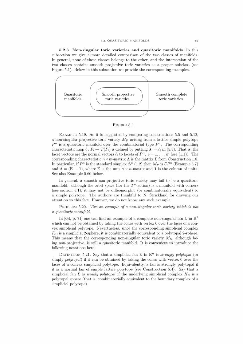
5.2. QUASITORIC MANIFOLDS 67
5.2.3. Non-singular toric varieties and quasitoric manifolds. In thissubsection we give a more detailed comparison of the two classes of manifolds.In general, none of these classes belongs to the other, and the intersection of thetwo classes contains smooth projective toric varieties as a proper subclass (seeFigure 5.1). Below in this subsection we provide the corresponding examples.
'
&
$
%
'
&
$
%
'
&
$
%
Quasitoricmanifolds
Smooth completetoric varieties
Smooth projectivetoric varieties
Figure 5.1.
Example 5.19. As it is suggested by comparing constructions 5.5 and 5.12,a non-singular projective toric variety MP arising from a lattice simple polytopePn is a quasitoric manifold over the combinatorial type Pn. The correspondingcharacteristic map ` : Fi 7→ T (Fi) is defined by putting λλi = l i in (5.3). That is, thefacet vectors are the normal vectors l i to facets of Pn, i = 1, . . . ,m (see (1.1)). Thecorresponding characteristic n×m-matrix Λ is the matrix L from Construction 1.8.In particular, if Pn is the standard simplex ∆n (1.2) then MP is CPn (Example 5.7)and Λ = (E | −1), where E is the unit n × n-matrix and 1 is the column of units.See also Example 5.60 below.
In general, a smooth non-projective toric variety may fail to be a quasitoricmanifold: although the orbit space (for the Tn-action) is a manifold with corners(see section 5.1), it may not be diffeomorphic (or combinatorially equivalent) toa simple polytope. The authors are thankful to N. Strickland for drawing ourattention to this fact. However, we do not know any such example.
Problem 5.20. Give an example of a non-singular toric variety which is nota quasitoric manifold.
In [64, p. 71] one can find an example of a complete non-singular fan Σ in R3
which can not be obtained by taking the cones with vertex 0 over the faces of a con-vex simplicial polytope. Nevertheless, since the corresponding simplicial complexKΣ is a simplicial 2-sphere, it is combinatorially equivalent to a polytopal 2-sphere.This means that the corresponding non-singular toric variety MΣ, although be-ing non-projective, is still a quasitoric manifold. It is convenient to introduce thefollowing notations here.
Definition 5.21. Say that a simplicial fan Σ in Rn is strongly polytopal (orsimply polytopal) if it can be obtained by taking the cones with vertex 0 over thefaces of a convex simplicial polytope. Equivalently, a fan is strongly polytopal ifit is a normal fan of simple lattice polytope (see Construction 5.4). Say that asimplicial fan Σ is weakly polytopal if the underlying simplicial complex KΣ is apolytopal sphere (that is, combinatorially equivalent to the boundary complex of asimplicial polytope).
68 5. TORIC AND QUASITORIC MANIFOLDS
Suppose Σ is a non-singular fan and MΣ the corresponding toric variety. ThenMΣ is projective if and only if Σ is strongly polytopal, and MΣ is a quasitoricmanifold if and only if Σ is weakly polytopal. Thus, the answer to Problem 5.20can be given by providing a non-singular fan which is not weakly polytopal. Asit was told to the authors by Y. Civan (in private communications), this maybe done by giving a (singular) fan Σ whose underlying simplicial complex KΣ isthe Barnette sphere (see section 2.3) and then desingularizing it using the standardprocedure (see [64, §2.6]). Combinatorial properties of the Barnette sphere obstructthe resulting (non-singular) fan to be weakly polytopal.
On the other hand, it is easy to construct a quasitoric manifold which is not atoric variety. The simplest example is the manifold CP 2 #CP 2, the connected sumof two copies of CP 2. It is a quasitoric manifold over the square I2 (this followsfrom the construction of equivariant connected sum, see [48, 1.11] or section 5.3 andcorollary 5.66 below). However, CP 2 #CP 2 do not admit even an almost complexstructure (i.e., its tangent bundle cannot be made complex). The following problemarises.
Problem 5.22. Let (Pn, `) be a characteristic pair (see Definition 5.11), andM2n(`) the derived quasitoric manifold (see Construction 5.12). Find conditionson Pn and ` so that M2n(`) admits a Tn-invariant complex (or almost complex)structure.
The almost complex case of the above problem was formulated in [48, Prob-lem 7.6]. Since every non-singular toric variety is a complex manifold, characteristicpairs coming from lattice simple polytopes (as described in Example 5.19) providea sufficient condition for Problem 5.22. However, this is not a necessary conditioneven for the existence of an invariant complex structure. Indeed, there exist smoothnon-projective toric varieties coming from weakly polytopal fans (see the alreadymentioned example in [64, p. 71]). At the same time, we do not know any exampleof non-toric complex quasitoric manifold.
Problem 5.23. Find an example of a non-toric quasitoric manifold that admitsa Tn-invariant complex structure.
Although a general quasitoric manifold may fail to be complex or almost com-plex, it always admits a Tn-invariant complex structure in the stable tangent bun-dle. The corresponding constructions are the subject of next section. We will returnto Problem 5.22 in subsection 5.4.2.
Another class of problems arises in connection with the classification of qua-sitoric manifolds over a given combinatorial simple polytope. The general settingof this problem is discussed in section 5.5. Example 5.26 below shows that thereare combinatorial simple polytopes that do not admit a characteristic map (andtherefore can not arise as orbit spaces for quasitoric manifolds).
Problem 5.24. Give a combinatorial description of the class of polytopes Pn
that admit a characteristic map (5.4).
A generalization of this problem is considered in chapter 7 (Problem 7.27).A characteristic map is determined by an integer n×m-matrix Λ which satis-
fies (5.5) for every vertex v ∈ Pn. The equation (det Λ(v))2 = 1 defines a hypersur-face in the space M(n,m;Z) of integer n×m-matrices.
5.3. STABLY COMPLEX STRUCTURES AND COBORDISMS 69
Proposition 5.25. The set of characteristic matrices coincides with the inter-section
(5.7)⋂
v∈P n
(detΛ(v))2 = 1
of hypersurfaces in the space M(n,m;Z), where v is running through the verticesof the polytope Pn.
Thus, Problem 5.24 is to determine for which polytopes the intersection in (5.7)is non-empty.
Example 5.26 ([48, Example 1.22]). Let Pn be a 2-neighborly simple polytopewith m ≥ 2n facets (e.g., the polar of cyclic polytope Cn(m) with n ≥ 4 andm ≥ 2n, see Example 1.17). Then this Pn does not admit a characteristic map andtherefore can not appear as the quotient space of a quasitoric manifold. Indeed, byProposition 5.25, it is sufficient to show that intersection (5.7) is empty. Since m ≥2n, any matrix Λ ∈ M(n,m;Z) (without zero columns) contains two columns, sayi-th and j-th, which coincide modulo 2. Since Pn is 2-neighborly, the correspondingfacets Fi and Fj have non-empty intersection in Pn. Hence, the columns i and jof Λ enter the minor Λ(v) for some vertex v ∈ Pn. This implies that the determinantof this minor is even and intersection (5.7) is empty.
In particular, the above example implies that there are no non-singular toricvarieties over the combinatorial polar cyclic polytope (Cn(m))∗ with ≥ 2n facets.This means that the combinatorial type Cn(m) with m ≥ 2n can not be realizedas a lattice simplicial polytope in such a way that the fan over its faces is non-singular. In the toric geometry, the question of whether for any given completesimplicial fan Σ there exists a combinatorially equivalent fan Σ′ that gives riseto a smooth toric variety was known as Ewald’s conjecture of 1986. The firstcounterexample was found in [67]. It was shown there that no fan over the facesof a lattice realization of Cn(m) with m ≥ n + 3 is non-singular. The comparisonof this result with Example 5.26 suggests that some cyclic polytopes Cn(m) withsmall number of vertices (between n + 3 and 2n) may appear as the quotients ofquasitoric manifolds, but not as quotients of non-singular toric varieties.
Another interesting corollary of Example 5.26 is that the face ring Z(Cn(m))of (the boundary complex of) Cn(m) and the face ring Z/p(Cn(m)) for any primep does not admit a regular sequence of degree two (or a lsop). Of course, sinceZ/p(Cn(m)) is Cohen–Macaulay, it admits a non-linear regular sequence. Notethat in the case when k is of zero characteristic the ring k(Cn(m)) always admitsa lsop (and degree-two regular sequence) by Lemma 3.11.
5.3. Stably complex structures, and quasitoric representatives incobordism classes
This section is the review of results obtained by N. Ray and the first authorin [37] and [38], supplied with some additional comments.
A stably complex structure on a (smooth) manifold M is determined by a com-plex structure in the vector bundle τ(M) ⊕ Rk for some k, where τ(M) is thetangent bundle of M and Rk denotes a trivial real k-dimensional bundle over M .A stably complex manifold (in other notations, weakly almost complex manifold orU -manifold) is a manifold with fixed stably complex structure, which one can view
70 5. TORIC AND QUASITORIC MANIFOLDS
as a pair (M, ξ), where ξ is a complex bundle isomorphic, as a real bundle, toτ(M) ⊕ Rk for some k. If M itself is a complex manifold, then it possesses thecanonical stably complex structure (M, τ(M)). The operations of disjoint unionand product endow the set of cobordism classes [M, ξ] of stably complex manifoldswith the structure of a graded ring, called the complex cobordism ring ΩU . By thetheorem of Milnor and Novikov, the complex cobordism ring is isomorphic to thepolynomial ring on infinite number of even-dimensional generators:
ΩU ∼= Z[a1, a2, . . .], deg ai = 2i,
(see [104], [130]). The ring ΩU is the coefficient ring for generalized (co)homologytheory known as the complex (co)bordisms. We refer to [130] as the standard sourcefor the cobordism theory.
Stably complex manifolds was the main subject of F. Hirzebruch’s talk at the1958 International Congress of mathematicians, see [135]. Using Milnor hypersur-faces (Example 5.39) and the Milnor–Novikov theorem it was shown by Milnor [135]that every complex cobordism class contains a non-singular algebraic variety, notnecessarily connected. The following problem is still open.
Problem 5.27 (Hirzebruch). Which complex cobordism classes in ΩU containconnected non-singular algebraic varieties?
A weaker version of this question, which is also open, asks which cobordismclasses contain connected almost complex manifolds.
Example 5.28. The 2-dimensional cobordism group ΩU2∼= Z is generated by
the class of [CP 1] (Riemannian sphere). Every cobordism class k[CP 1] ∈ ΩU2
contains a non-singular algebraic variety, namely, the disjoint union of k copies ofCP 1 for k > 0 and a Riemannian surface of genus (1 − k) for k ≤ 0. However,connected algebraic varieties are contained only in the cobordism classes k[CP 1]with k ≤ 1.
The problem of choosing appropriate generators for the ring ΩU is very impor-tant in the cobordism theory and its applications. As it has been recently shownin [37] and [38], every complex cobordism class (of dimension > 2) contains aquasitoric manifold (see Theorem 5.38 below). By the definition, quasitoric man-ifolds are necessarily connected, so the result may be considered as an answer tothe quasitoric analogue of Hirzebruch’s question. The construction of quasitoricrepresentatives in complex cobordism classes relies upon an additional structureon a quasitoric manifold, called omniorientation, which provides a combinatorialdescription for canonical stably complex structures.
Let π : M2n → Pn be a quasitoric manifold with characteristic map `. Sincethe torus Tn (5.1) is oriented, a choice of orientation for Pn is equivalent to a choiceof orientation for M2n. (An orientation of Pn is specified by orienting the ambientspace Rn.)
Definition 5.29. An omniorientation of a quasitoric manifold M2n consistsof a choice of an orientation for M2n and for every facial submanifold M
2(n−1)i =
π−1(Fi), i = 1, . . . , m.
Thus, there are 2m+1 omniorientations in all for given M2n.An omniorientation of M2n determines an orientation for every normal bundle
νi := ν(Mi ⊂ M2n), i = 1, . . . ,m. Since every νi is a real 2-plane bundle, an
5.3. STABLY COMPLEX STRUCTURES AND COBORDISMS 71
orientation of νi allows to interpret it as a complex line bundle. The isotropysubgroup T (Fi) (see (5.3)) of submanifold M
2(n−1)i = π−1(Fi) acts on the normal
bundle νi, i = 1, . . . , m. Thus, we have the following statement.
Proposition 5.30. A choice of omniorientation for M2n is equivalent to achoice of orientation for Pn together with an unambiguous choice of facet vectorsλλi, i = 1, . . . , m in (5.3).
We refer to a characteristic map ` as directed if all circles `(Fi), i = 1, . . . , m,are oriented. This implies that the signs of facet vectors λλi = (λ1i, . . . , λni)t,i = 1, . . . , m, are determined unambiguously. In the previous section we organizedthe facet vectors into the integer n × m matrix Λ. This matrix satisfies (5.5).Due to (5.3), the matrix Λ carries exactly the same information as a directedcharacteristic map. Let ZF denote the m-dimensional free Z-module spanned by theset F of facets of Pn. Then Λ defines an epimorphism λ : ZF → Zn by λ(Fi) = λλi
and an epimorphism TF → Tm, which we will denote by the same letter λ. In thesequel we write Zm for ZF and Tm for TF , assuming that the member e i of thestandard basis of Zm corresponds to the facet Fi ∈ ZF , i = 1, . . . , m, and similarlyfor Tm.
Definition 5.31. A directed characteristic pair (Pn,Λ) consists of a combina-torial simple polytope Pn and an integer matrix Λ (or, equivalently, an epimorphismλ : Zm → Zn) that satisfies (5.5).
Proposition 5.30 shows that the characteristic pair of an omnioriented quasitoricmanifold is directed. On the other hand, the quasitoric manifold derived from adirected characteristic pair using Construction 5.12 is omnioriented.
Construction 5.32. The orientation of the normal bundle νi over Mi de-fines an integral Thom class in the cohomology group H2(T (νi)), represented bya complex line bundle over the Thom complex T (νi). We pull this back along thePontryagin–Thom collapse M2n → T (νi), and denote the resulting bundle ρi. Therestriction of ρi to Mi ⊂ M2n is νi. In the algebraic geometry this constructioncorresponds to assigning the line bundle to a divisor. In particular, in the casewhen M2n is a smooth toric variety, the line bundle ρi corresponds to the divisorDi, see Theorem 5.3.
Theorem 5.33 ([48] and [38, Theorem 3.8]). Every omniorientation of a qu-asitoric manifold M2n determines a stably complex structure on it by means of thefollowing isomorphism of real 2m-bundles:
τ(M2n)⊕ R2(m−n) ∼= ρ1 ⊕ · · · ⊕ ρm.
The above isomorphism of real vector bundles is essentially due to Davis andJanuszkiewicz (see [48, Theorem 6.6]). The interpretation of stably complex struc-tures in terms of omniorientations was given in [38].
Corollary 5.34. In the notations of Theorem 5.18, suppose vi ∈ H2(M2n) isthe cohomology class dual to the oriented facial submanifold Mi of an omniorientedquasitoric manifold M2n, i = 1, . . . , m. Then the total Chern class of stablycomplex structure on M2n defined by the omniorientation is given by
c(M2n) = (1 + v1) . . . (1 + vm) ∈ H∗(M2n).
72 5. TORIC AND QUASITORIC MANIFOLDS
It follows from Theorem 5.33 that a directed characteristic pair (Pn,Λ) deter-mines a complex cobordism class [M2n, ρ1 ⊕ · · · ⊕ ρm] ∈ ΩU . The following directextension of Theorem 5.18 provides a description of the complex cobordism ring ofan omnioriented quasitoric manifold.
Proposition 5.35 ([38, Proposition 5.3]). Let vi denote the first cobordismChern class c1(ρi) ∈ Ω2
U (M2n) of the bundle ρi, 1 ≤ i ≤ m. Then the complexcobordism ring of M2n is given by
Ω∗U (M2n) = ΩU [v1, . . . , vm]/(IP + JΛ),
where the ideals IP and JΛ are defined in the same way as in Theorem 5.18.
Note that the Chern class c1(ρi) is Poincare dual to the inclusion M2(n−1)i ⊂ M2n
by the construction of ρi. This highlights the remarkable fact that the complexbordism groups ΩU
∗ (M2n) are spanned by embedded submanifolds. By definition,the fundamental cobordism class 〈M2n〉 ∈ Ω2n
U (M2n) is dual to the bordism class ofa point. Thus, 〈M2n〉 = vi1 · · · vin
for any set i1, . . . , in such that Fi1 ∩ · · · ∩ Fin
is a vertex of Pn.The following two examples are used to construct quasitoric representatives in
complex cobordisms.
Example 5.36 (bounded flag manifold [36]). A bounded flag in Cn+1 is acomplete flag U = U1 ⊂ U2 ⊂ · · · ⊂ Un+1 = Cn+1 for which Uk, 2 ≤ k ≤ n,contains the coordinate subspace Ck−1 spanned by the first k − 1 standard basisvectors. As it is shown in [38, Example 2.8], the 2n-dimensional manifold Bn ofall bounded flags in Cn+1 is a quasitoric manifold over the combinatorial cube In
with respect to the action induced by t · z = (t1z1, . . . , tnzn, zn+1) on Cn+1, wheret ∈ Tn.
Example 5.37. A family of manifolds Bi,j (0 ≤ i ≤ j) is introduced in [37].The manifold Bi,j consists of pairs (U,W ), where U is a bounded flag in Ci+1 (seeExample 5.36) and W is a line in U⊥
1 ⊕ Cj−i. So Bi,j is a smooth CP j−1-bundleover Bi. It is shown in [38, Example 2.9] that Bi,j is a quasitoric manifold over theproduct Ii ×∆j−1.
The canonical stably complex structures and omniorientations on the manifoldsBn and Bi,j are described in [38, examples 4.3, 4.5].
Remark. The product of two quasitoric manifolds M2n11 and M2n2
2 over poly-topes Pn1
1 and Pn22 is a quasitoric manifold over Pn1
1 × Pn22 . This construction
extends to omnioriented quasitoric manifolds and is compatible with stably com-plex structures (details can be found in [38, Proposition 4.7]).
It is shown in [37] that the cobordism classes of Bi,j multiplicatively gener-ate the ring ΩU . Hence, every 2n-dimensional complex cobordism class may berepresented by a disjoint union of products
(5.8) Bi1,j1 ×Bi2,j2 × · · · ×Bik,jk,
where∑k
q=1(iq + jq) − 2k = n. Each such component is a quasitoric manifold,under the product quasitoric structure. This result is the substance of [37]. Thestably complex structures of products (5.8) are induced by omniorientations, andare therefore also preserved by the torus action.
5.3. STABLY COMPLEX STRUCTURES AND COBORDISMS 73
To give genuinely quasitoric representatives (which are, by definition, con-nected) for each cobordism class of dimension > 2, it remains only to replace thedisjoint union of products (5.8) with their connected sum. This is done in [38, §6]using Construction 1.13 and its extension to omnioriented quasitoric manifolds.
Theorem 5.38 ([38, Theorem 6.11]). In dimensions > 2, every complex cobor-dism class contains a quasitoric manifold, necessarily connected, whose stably com-plex structure is induced by an omniorientation, and is therefore compatible withthe action of the torus.
The connected sum operation usually destroys the algebraicity of manifolds, sothe complex cobordism representatives provided by the above theorem in generalare not algebraic (compare Example 5.28).
We note that in their work [44, §42] Conner and Floyd constructed a class ofmanifolds with canonical circle actions which can be chosen as representatives formultiplicative generators in oriented cobordisms. One can show that these Conner–Floyd manifolds can be obtained as particular cases of manifolds Bi,j from Exam-ple 5.37. However, Conner and Floyd did not consider actions of half-dimensionaltori on their manifolds.
Example 5.39. The standard set of multiplicative generators for ΩU consistsof projective spaces CP i, i ≥ 0, and Milnor hypersurfaces Hi,j ⊂ CP i × CP j ,1 ≤ i ≤ j. The hypersurface Hi,j is defined by
Hi,j =
(z0 : · · · : zi)× (w0 : · · · : wj) ∈ CP i × CP j :i∑
q=0
zqwq = 0
.
However, the hypersurfaces Hi,j are not quasitoric manifolds for i > 1, see [37].This can be shown in the following way.
Construction 5.40. Let Ci+1 ⊂ Cj+1 be the subspace spanned by the firsti + 1 vectors of the standard basis of Cj+1. Identify CP i with the set of complexlines l ⊂ Ci+1. To each line l assign the set of hyperplanes α ⊂ Cj+1 that contain l.The latter set is identified with CP j−1, so there is a bundle E → CP i with fibreCP j−1. Here E is the set of pairs (l, α), l ⊂ α, and the projection takes (l, α) to l.
Lemma 5.41. Hi,j is identified with the total space of bundle E → CP i.
Proof. A line l ⊂ Ci+1 is given by a vector (z0 : z1 : · · · : zi). A hyperplaneα ⊂ Cj+1 is given by a linear form. If we denote the coefficients of this linear formby w0, w1, . . . , wj , then the condition l ⊂ α is exactly that from the definition ofHi,j . ¤
Theorem 5.42. The cohomology of Hi,j is given by
H∗(Hi,j) ∼= Z[u, v]/(
ui+1 = 0, vj−ii∑
k=0
ukvi−k = 0),
where deg u = deg v = 2.
Proof. We will use the notations from Construction 5.40. Let ζ denote thebundle over CP i whose fibre over l ∈ CP i is the j-dimensional subspace l⊥ ⊂ Cj+1.Then one can identify Hi,j with the projectivization CP (ζ). Indeed, for any linel′ ⊂ l⊥ representing a point in the fibre of CP (ζ) over l ∈ CP i the hyperplane
74 5. TORIC AND QUASITORIC MANIFOLDS
α = (l′)⊥ ⊂ Cj+1 contains l, so the pair (l, α) represents a point in Hi,j (seeLemma 5.41). The rest of the proof reproduces the general argument from theDold theorem about the cohomology of projectivizations.
Denote by ξ the tautological line bundle over CP i (its fibre over l ∈ CP i is theline l itself). Then ξ ⊕ ζ is a trivial (j + 1)-dimensional bundle. Set w = c1(ξ) ∈H2(CP i). Let c(ξ) = 1 + c1(ξ) + c2(ξ) + . . . denote the total Chern class. Sincec(ξ)c(ζ) = 1 and c(ξ) = 1− w, we get
(5.9) c(ζ) = 1 + w + · · ·+ wi.
Consider the projection p : CP (ζ) → CP i. Denote by η the “tautological”line bundle over CP (ζ) whose fiber over a point l′ ∈ CP (ζ) is the line l′ itself.Denote by η⊥ the (j − 1)-bundle over CP (ζ) whose fibre over a point l′ ⊂ l⊥ is theorthogonal complement to l′ in l⊥. Then it is easy to see that p∗(ζ) = η ⊕ η⊥. Setv = c1(η) ∈ H2(CP (ζ)) and u = p∗(w) ∈ H2(CP (ζ)). Then ui+1 = 0. We havec(η) = 1− v and c(p∗(ζ)) = c(η)c(η⊥), hence,
c(η⊥) = p∗(c(ζ)
)(1− v)−1 = (1 + u + · · ·+ ui)(1 + v + v2 + . . . )
(see (5.9)). But η⊥ is (j − 1)-dimensional, hence cj(η⊥) = 0. Calculating thehomogeneous part of degree j in the above identity, we get the second identity0 = vj−i
∑ik=0 ukvi−k.
Since both CP i and CP j−1 have only even-dimensional cells, the Leray–Serrespectral sequence of the bundle p : CP (ζ) → CP i collapses at the E2 term. Itfollows that there is an epimorphism Z[u, v] → H∗(CP (ζ)), and additively thecohomology of H∗(CP (ζ)) coincides with that of CP i × CP j−1. Hence, there areno other relations except those two mentioned in the theorem. ¤
Proposition 5.43. Hi,j is not a quasitoric manifold for i > 1.
Proof. By theorem 5.18, the cohomology of a quasitoric manifold is isomor-phic to a quotient Z[v1, . . . , vm]/I+J , where the ideal I is generated by square-freemonomials and J is generated by linear forms. Due to (5.5) we may assume withoutloss of generality that first n variables v1, . . . , vn are expressed via the last m − nby means of linear equations with integer coefficients. Hence, we have
Z[v1, . . . , vm]/I+J ∼= Z[w1, . . . , wm−n]/I ′,where I ′ is an ideal having a basis each of whose elements is a product of ≥ 2integer linear forms. Suppose now that Hi,j , i > 1, is a quasitoric manifold. Thenwe have an isomorphism
Z[w1, . . . , wm−n]/I ′ ∼= Z[u, v]/I ′′,where I ′′ is the ideal from Theorem 5.42. It is easy to see that in this case we havem − n = 2 above, and w1, w2 can be identified with u, v. Thus, the ideal I ′′ musthave a basis consisting of products of ≥ 2 linear forms with integer coefficients. Butthis is impossible for i > 1. ¤
5.4. Combinatorial formulae for Hirzebruch genera of quasitoricmanifolds
The constructions from previous section open the way to evaluation of cobor-dism invariants (Chern numbers, Hirzebruch genera etc.) on omnioriented qua-sitoric manifolds in terms of the combinatorics of the quotient. In this section we
5.4. HIRZEBRUCH GENERA OF QUASITORIC MANIFOLDS 75
expose the results obtained in this direction by the second author in [111], [112].Namely, using arguments similar to that from the proof of Theorem 1.20 we con-struct a circle action with only isolated fixed points on any quasitoric manifold M2n.If M2n is omnioriented then this action preserves the stably complex structure andits local representations near fixed points are described in terms of the characteristicmatrix Λ. This allows to calculate Hirzebruch’s χy-genus as a sum of contributionscorresponding to the vertices of polytope. Each of these contributions depends onlyon the “local combinatorics” near the vertex. In particular, our formula allows tocalculate the signature and the Todd genus of M2n.
Definition 5.44. The Hirzebruch genus [74], [75] associated with the series
Q(x) = 1 +∑
qkxk, qk ∈ Q,
is the ring homomorphism ϕQ : ΩU → Q that to each cobordism class [M2n] ∈ ΩU2n
assigns the value given by the formula
ϕQ[M2n] =( n∏
i=1
Q(xi), 〈M2n〉).
Here M2n is a smooth manifold whose stable tangent bundle τ(M2n) is a complexbundle with complete Chern class in cohomology
c(τ) = 1 + c1(τ) + · · ·+ cn(τ) =n∏
i=1
(1 + xi),
and 〈M2n〉 is the fundamental class in homology.
As it was shown by Hirzebruch, every ring homomorphism ϕ : ΩU → Q arisesas a genus ϕQ for some Q. There is also an oriented version of Hirzebruch genera,which deals with ring homomorphisms ϕ : ΩSO → Q from the oriented cobordismring ΩSO.
Definition 5.45. The χy-genus is the Hirzebruch genus associated with theseries
Q(x) =x(1 + ye−x(1+y))
1− e−x(1+y),
where y ∈ R is a parameter. For particular values y = −1, 0, 1 we obtain the n-thChern number, the Todd genus and the L-genus of M2n correspondingly.
Given a 4k-dimensional oriented manifold X4k, the signature sign(X4k) is de-fined as the signature (the number of positive squares minus the number of negativeones) of the intersection form
f(α, β) :=(α · β, 〈X4k〉), α, β ∈ H2k(X4k)
in the middle-dimensional cohomology H2k(X4k). We also extend the signatureto all even-dimensional manifolds by setting sign(X4k+2) = 0. It can be shownthat the signature is multiplicative and is an invariant of cobordism, so it definesa ring homomorphism ϕ : ΩSO → Z (a genus). By the classical theorem of Hirze-bruch [74], the signature coincides with the L-genus, and we will not distinguishbetween the two notions in the sequel.
In the case when M2n is a complex manifold, the value χy(M2n) can be calcu-lated in terms of Euler characteristics of the Dolbeault complexes on M2n, see [74].This was the original Hirzebruch’s motivation for studying the χy-genus.
76 5. TORIC AND QUASITORIC MANIFOLDS
In this section we assume that we are given an omnioriented quasitoric manifoldM2n over some Pn with characteristic matrix Λ. This specifies a stably complexstructure on M2n, as described in the previous section. The orientation of M2n
determines the fundamental class 〈M2n〉 ∈ H2n(M2n;Z).
5.4.1. The sign and index of a vertex, edge vectors and calculationof the χy-genus. Here we introduce some combinatorial invariants of the torusaction and calculate the χy-genus.
Construction 5.46. Suppose v is a vertex of Pn expressed as the intersectionof n facets:
(5.10) v = Fi1 ∩ · · · ∩ Fin .
To each facet Fikabove assign the unique edge Ek such that Ek ∩ Fik
= v (thatis, Ek =
⋂j 6=k Fij
). Let ek be a vector along Ek with origin v. Then e1, . . . , en isa basis of Rn, which may be either positively or negatively oriented depending onthe ordering of facets in (5.10). Throughout this section we assume this orderingto be so that e1, . . . , en is a positively oriented basis.
Once we specified an ordering of facets in (5.10), the facet vectors λλi1 , . . . , λλin
at v may in turn constitute either positively or negatively oriented basis dependingon the sign of the determinant of Λ(v) = (λλi1 , . . . , λλin) (see (5.5)).
Definition 5.47. The sign of a vertex v = Fi1 ∩ · · · ∩ Fin is
σ(v) := det Λ(v).
One can understand the sign of a vertex geometrically as follows. For eachvertex v ∈ Pn the omniorientation of M2n determines two orientations of thetangent space TvM2n at v. The first is induced by the orientation of M2n. On theother hand, TvM2n decomposes into the sum of n two-dimensional vector spacesnormal to the facial submanifolds Mi1 , . . . , Min containing v. By the definition ofomniorientation, each of these two-dimensional vector spaces is oriented, so theytogether define another orientation of TvM2n. Then σ(v) = 1 if the two orientationscoincide and σ(v) = −1 otherwise.
The collection of signs of vertices of Pn is an important invariant of an omnior-iented quasitoric manifold. Note that reversing the orientation of M2n changes allsigns σ(v) to the opposite. At the same time changing the direction of one facetvector reverses the signs for those vertices contained in the corresponding facet.
Let E be an edge of Pn. The isotropy subgroup of 2-dimensional submanifoldπ−1(E) ⊂ M2n is an (n − 1)-dimensional subtorus, which we denote by T (E). Itcan be written as
(5.11) T (E) =(
e2πiϕ1 , . . . , e2πiϕn) ∈ Tn : µ1ϕ1 + . . . + µnϕn = 0
for some integers µ1, . . . , µn. We refer to µµ := (µ1, . . . , µn)t as the edge vectorcorresponding to E. This µµ is a primitive vector in the dual lattice (Zn)∗ and isdetermined by E only up to a sign. There is no canonical way to choose thesesigns simultaneously for all edges. However, the following lemma shows that theomniorientation of M2n provides a canonical way to choose signs of edge vectors“locally” at each vertex.
5.4. HIRZEBRUCH GENERA OF QUASITORIC MANIFOLDS 77
Lemma 5.48. For each vertex v ∈ Pn, the signs of edge vectors µµ1, . . . , µµn
meeting at v can be chosen in such way that the n× n-matrix M(v) := (µµ1, . . . , µµn)satisfies the identity
Mt(v) · Λ(v) = E,
where E is the unit matrix. In other words, µµ1, . . . , µµn and λλi1 , . . . , λλinare conju-
gate bases.
Proof. At the beginning we choose signs of the edge vectors at v arbitrary,and express v as in (5.10). Then µµk is the edge vector corresponding to the edge Ek
opposite to Fik, k = 1, . . . , n. It follows that Ek ⊂ Fil
for l 6= k, so T (Fil) ⊂ T (Ek).
Hence,
(5.12) 〈µµk, λλil〉 = 0, l 6= k,
(see (5.3) and (5.11)). Since µµk is a primitive vector and λλi1 , . . . , λλinis a basis of
Zn, it follows from (5.12) that 〈µµk, λλik〉 = ±1. Changing the sign of µµik
if necessary,we obtain
〈µµk, λλik〉 = 1,
which together with (5.12) gives Mt(v) · Λ(v) = E, as needed. ¤
In the sequel, while making some local calculations near a vertex v, we assumethat the signs of edge vectors are chosen as in the above lemma. It follows that theedge vectors µµ1, . . . , µµn meeting at v constitute an integer basis of Zn and
(5.13) det M(v) = σ(v).
Example 5.49. Suppose M2n = MP is a smooth toric variety arising froma lattice simple polytope P defined by (1.1). Then λλi = l i, i = 1, . . . , m (seeExample 5.19), whereas the edge vectors at v ∈ Pn are the primitive integer vectorse1, . . . , en along the edges with origin at v. It follows from Construction 5.46 thatσ(v) = 1 for any v (compare with Proposition 5.53 below). Lemma 5.48 in thiscase expresses the fact that e1, . . . , en and l i1 , . . . , l in are conjugate bases of Zn.
Remark. Globally Lemma 5.48 provides two directions (signs) for an edgevector, one for each of its ends. These two signs are always different if M2n is acomplex manifold (e.g. a smooth toric variety), but in general they may the sameas well.
Let νν = (ν1, . . . , νn)t ∈ Zn be a primitive vector such that
(5.14) 〈µµ, νν〉 6= 0 for any edge vector µµ.
The vector νν defines a one-dimensional oriented subtorus:
Tνν :=(
e2πiν1ϕ, . . . , e2πiνnϕ) ∈ Tn , ϕ ∈ R
.
Lemma 5.50 ([112, Theorem 2.1]). For any νν satisfying (5.14) the circle Tνν
acts on M2n with only isolated fixed points, corresponding to the vertices of Pn.For each vertex v = Fi1 ∩ · · · ∩ Fin the action of Tνν induces a representation of S1
in the tangent space TvM2n with weights 〈µµ1, νν〉, . . . , 〈µµn, νν〉.Remark. If M2n = MP is a smooth toric variety, then the genericity condi-
tion (5.14) is equivalent to that from the proof of Theorem 1.20.
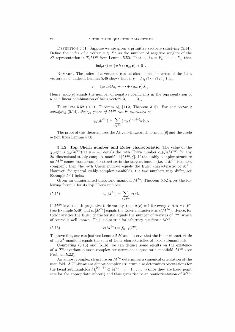
78 5. TORIC AND QUASITORIC MANIFOLDS
Definition 5.51. Suppose we are given a primitive vector νν satisfying (5.14).Define the index of a vertex v ∈ Pn as the number of negative weights of theS1-representation in TvM2n from Lemma 5.50. That is, if v = Fi1 ∩ · · · ∩ Fin
then
indνν(v) = #k : 〈µµk, νν〉 < 0.Remark. The index of a vertex v can be also defined in terms of the facet
vectors at v. Indeed, Lemma 5.48 shows that if v = Fi1 ∩ · · · ∩ Finthen
νν = 〈µµ1, νν〉λλi1 + · · ·+ 〈µµn, νν〉λλin.
Hence, indνν(v) equals the number of negative coefficients in the representation ofνν as a linear combination of basis vectors λλi1 , . . . , λλin
.
Theorem 5.52 ([111, Theorem 6], [112, Theorem 3.1]). For any vector ννsatisfying (5.14), the χy-genus of M2n can be calculated as
χy(M2n) =∑
v∈P n
(−y)indν(v)σ(v).
The proof of this theorem uses the Atiyah–Hirzebruch formula [8] and the circleaction from Lemma 5.50.
5.4.2. Top Chern number and Euler characteristic. The value of theχy-genus χy(M2n) at y = −1 equals the n-th Chern number cn(ξ)〈M2n〉 for any2n-dimensional stably complex manifold [M2n, ξ]. If the stably complex structureon M2n comes from a complex structure in the tangent bundle (i.e. if M2n is almostcomplex), then the n-th Chern number equals the Euler characteristic of M2n.However, for general stably complex manifolds, the two numbers may differ, seeExample 5.61 below.
Given an omnioriented quasitoric manifold M2n, Theorem 5.52 gives the fol-lowing formula for its top Chern number:
(5.15) cn[M2n] =∑
v∈P n
σ(v).
If M2n is a smooth projective toric variety, then σ(v) = 1 for every vertex v ∈ Pn
(see Example 5.49) and cn[M2n] equals the Euler characteristic e(M2n). Hence, fortoric varieties the Euler characteristic equals the number of vertices of Pn, whichof course is well known. This is also true for arbitrary quasitoric M2n:
(5.16) e(M2n) = fn−1(Pn).
To prove this, one can just use Lemma 5.50 and observe that the Euler characteristicof an S1-manifold equals the sum of Euler characteristics of fixed submanifolds.
Comparing (5.15) and (5.16), we can deduce some results on the existenceof a Tn-invariant almost complex structure on a quasitoric manifold M2n (seeProblem 5.22).
An almost complex structure on M2n determines a canonical orientation of themanifold. A Tn-invariant almost complex structure also determines orientations forthe facial submanifolds M
2(n−1)i ⊂ M2n, i = 1, . . . , m (since they are fixed point
sets for the appropriate subtori) and thus gives rise to an omniorientation of M2n.
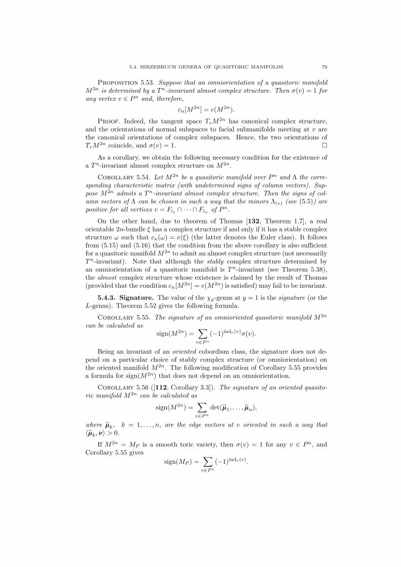
5.4. HIRZEBRUCH GENERA OF QUASITORIC MANIFOLDS 79
Proposition 5.53. Suppose that an omniorientation of a quasitoric manifoldM2n is determined by a Tn-invariant almost complex structure. Then σ(v) = 1 forany vertex v ∈ Pn and, therefore,
cn[M2n] = e(M2n).
Proof. Indeed, the tangent space TvM2n has canonical complex structure,and the orientations of normal subspaces to facial submanifolds meeting at v arethe canonical orientations of complex subspaces. Hence, the two orientations ofTvM2n coincide, and σ(v) = 1. ¤
As a corollary, we obtain the following necessary condition for the existence ofa Tn-invariant almost complex structure on M2n.
Corollary 5.54. Let M2n be a quasitoric manifold over Pn and Λ the corre-sponding characteristic matrix (with undetermined signs of column vectors). Sup-pose M2n admits a Tn-invariant almost complex structure. Then the signs of col-umn vectors of Λ can be chosen in such a way that the minors Λ(v) (see (5.5)) arepositive for all vertices v = Fi1 ∩ · · · ∩ Fin
of Pn.
On the other hand, due to theorem of Thomas [132, Theorem 1.7], a realorientable 2n-bundle ξ has a complex structure if and only if it has a stable complexstructure ω such that cn(ω) = e(ξ) (the latter denotes the Euler class). It followsfrom (5.15) and (5.16) that the condition from the above corollary is also sufficientfor a quasitoric manifold M2n to admit an almost complex structure (not necessarilyTn-invariant). Note that although the stably complex structure determined byan omniorientation of a quasitoric manifold is Tn-invariant (see Theorem 5.38),the almost complex structure whose existence is claimed by the result of Thomas(provided that the condition cn[M2n] = e(M2n) is satisfied) may fail to be invariant.
5.4.3. Signature. The value of the χy-genus at y = 1 is the signature (or theL-genus). Theorem 5.52 gives the following formula.
Corollary 5.55. The signature of an omnioriented quasitoric manifold M2n
can be calculated assign(M2n) =
∑
v∈P n
(−1)indν(v)σ(v).
Being an invariant of an oriented cobordism class, the signature does not de-pend on a particular choice of stably complex structure (or omniorientation) onthe oriented manifold M2n. The following modification of Corollary 5.55 providesa formula for sign(M2n) that does not depend on an omniorientation.
Corollary 5.56 ([112, Corollary 3.3]). The signature of an oriented quasito-ric manifold M2n can be calculated as
sign(M2n) =∑
v∈P n
det(µµ1, . . . , µµn),
where µµk, k = 1, . . . , n, are the edge vectors at v oriented in such a way that〈µµk, νν〉 > 0.
If M2n = MP is a smooth toric variety, then σ(v) = 1 for any v ∈ Pn, andCorollary 5.55 gives
sign(MP ) =∑
v∈P n
(−1)indν(v).
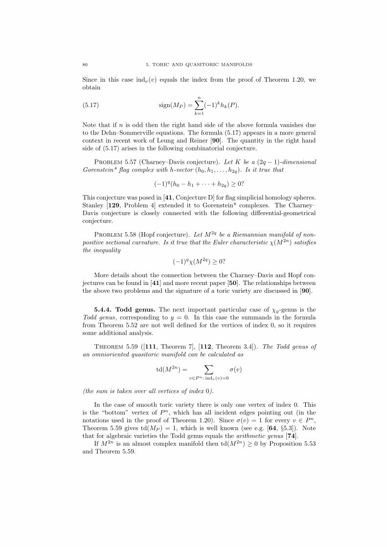
80 5. TORIC AND QUASITORIC MANIFOLDS
Since in this case indν(v) equals the index from the proof of Theorem 1.20, weobtain
(5.17) sign(MP ) =n∑
k=1
(−1)khk(P ).
Note that if n is odd then the right hand side of the above formula vanishes dueto the Dehn–Sommerville equations. The formula (5.17) appears in a more generalcontext in recent work of Leung and Reiner [90]. The quantity in the right handside of (5.17) arises in the following combinatorial conjecture.
Problem 5.57 (Charney–Davis conjecture). Let K be a (2q − 1)-dimensionalGorenstein* flag complex with h-vector (h0, h1, . . . , h2q). Is it true that
(−1)q(h0 − h1 + · · ·+ h2q) ≥ 0?
This conjecture was posed in [41, Conjecture D] for flag simplicial homology spheres.Stanley [129, Problem 4] extended it to Gorenstein* complexes. The Charney–Davis conjecture is closely connected with the following differential-geometricalconjecture.
Problem 5.58 (Hopf conjecture). Let M2q be a Riemannian manifold of non-positive sectional curvature. Is it true that the Euler characteristic χ(M2n) satisfiesthe inequality
(−1)qχ(M2q) ≥ 0?
More details about the connection between the Charney–Davis and Hopf con-jectures can be found in [41] and more recent paper [50]. The relationships betweenthe above two problems and the signature of a toric variety are discussed in [90].
5.4.4. Todd genus. The next important particular case of χy-genus is theTodd genus, corresponding to y = 0. In this case the summands in the formulafrom Theorem 5.52 are not well defined for the vertices of index 0, so it requiressome additional analysis.
Theorem 5.59 ([111, Theorem 7], [112, Theorem 3.4]). The Todd genus ofan omnioriented quasitoric manifold can be calculated as
td(M2n) =∑
v∈P n: indν(v)=0
σ(v)
(the sum is taken over all vertices of index 0).
In the case of smooth toric variety there is only one vertex of index 0. Thisis the “bottom” vertex of Pn, which has all incident edges pointing out (in thenotations used in the proof of Theorem 1.20). Since σ(v) = 1 for every v ∈ Pn,Theorem 5.59 gives td(MP ) = 1, which is well known (see e.g. [64, §5.3]). Notethat for algebraic varieties the Todd genus equals the arithmetic genus [74].
If M2n is an almost complex manifold then td(M2n) ≥ 0 by Proposition 5.53and Theorem 5.59.
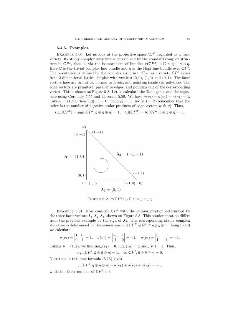
5.4. HIRZEBRUCH GENERA OF QUASITORIC MANIFOLDS 81
5.4.5. Examples.
Example 5.60. Let us look at the projective space CP 2 regarded as a toricvariety. Its stably complex structure is determined by the standard complex struc-ture in CP 2, that is, via the isomorphism of bundles τ(CP 2) ⊕ C ' η ⊕ η ⊕ η.Here C is the trivial complex line bundle and η is the Hopf line bundle over CP 2.The orientation is defined by the complex structure. The toric variety CP 2 arisesfrom 2-dimensional lattice simplex with vertices (0, 0), (1, 0) and (0, 1). The facetvectors here are primitive, normal to facets, and pointing inside the polytope. Theedge vectors are primitive, parallel to edges, and pointing out of the correspondingvertex. This is shown on Figure 5.2. Let us calculate the Todd genus and the signa-ture using Corollary 5.55 and Theorem 5.59. We have σ(v1) = σ(v2) = σ(v3) = 1.Take ν = (1, 2), then ind(v1) = 0, ind(v2) = 1, ind(v3) = 2 (remember that theindex is the number of negative scalar products of edge vectors with ν). Thus,
sign(CP 2) = sign(CP 2, η ⊕ η ⊕ η) = 1, td(CP 2) = td(CP 2, η ⊕ η ⊕ η) = 1.
@@
@@
@@
@@
@@
@@
@
"!
þ
v1 (1, 0) (−1, 0) v2
λλ2 = (0, 1)
(0, 1)
λλ1 = (1, 0)
(0,−1)
v3
(1,−1)
(−1, 1)
λλ3 = (−1,−1)
Figure 5.2. τ(CP 2)⊕ C ' η ⊕ η ⊕ η
Example 5.61. Now consider CP 2 with the omniorientation determined bythe three facet vectors λλ1, λλ2, λλ3, shown on Figure 5.3. This omniorientation differsfrom the previous example by the sign of λλ3. The corresponding stably complexstructure is determined by the isomorphism τ(CP 2)⊕R2 ∼= η⊕ η⊕ η. Using (5.13)we calculate
σ(v1) =∣∣∣∣1 00 1
∣∣∣∣ = 1, σ(v2) =∣∣∣∣−1 11 0
∣∣∣∣ = −1, σ(v3) =∣∣∣∣0 11 −1
∣∣∣∣ = −1.
Taking νν = (1, 2), we find indν(v1) = 0, indν(v2) = 0, indν(v3) = 1. Thus,
sign[CP 2, η ⊕ η ⊕ η] = 1, td[CP 2, η ⊕ η ⊕ η] = 0.
Note that in this case formula (5.15) gives
cn[CP 2, η ⊕ η ⊕ η] = σ(v1) + σ(v2) + σ(v3) = −1,
while the Euler number of CP 2 is 3.
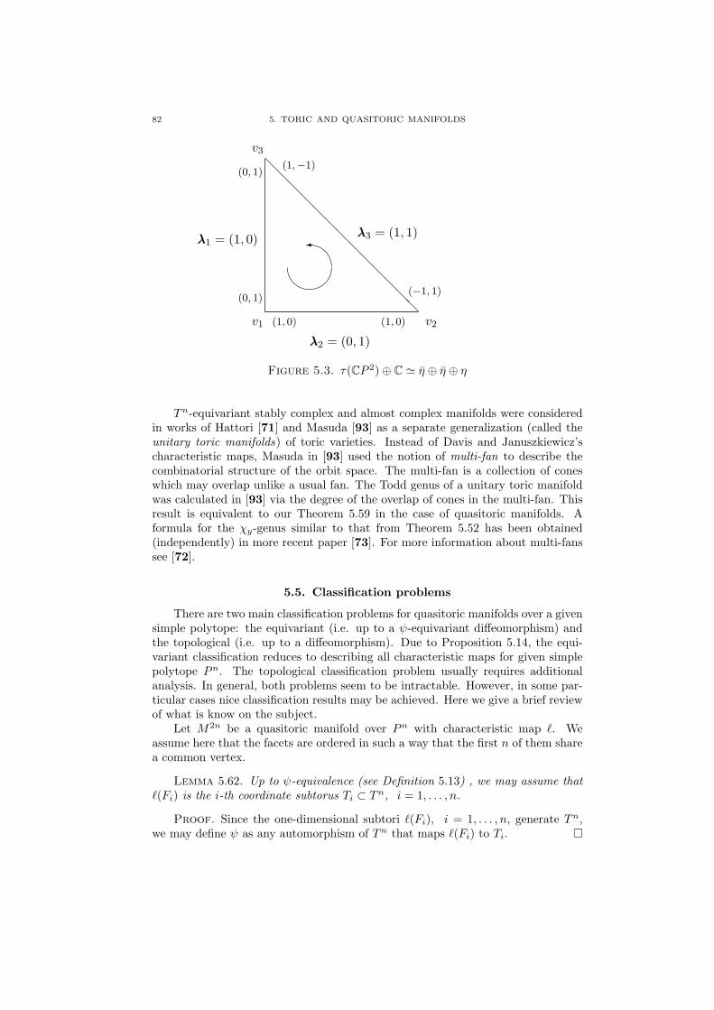
82 5. TORIC AND QUASITORIC MANIFOLDS
@@
@@
@@
@@
@@
@@
@
"!
þ
v1 (1, 0) (1, 0) v2
λλ2 = (0, 1)
(0, 1)
λλ1 = (1, 0)
(0, 1)
v3
(1,−1)
(−1, 1)
λλ3 = (1, 1)
Figure 5.3. τ(CP 2)⊕ C ' η ⊕ η ⊕ η
Tn-equivariant stably complex and almost complex manifolds were consideredin works of Hattori [71] and Masuda [93] as a separate generalization (called theunitary toric manifolds) of toric varieties. Instead of Davis and Januszkiewicz’scharacteristic maps, Masuda in [93] used the notion of multi-fan to describe thecombinatorial structure of the orbit space. The multi-fan is a collection of coneswhich may overlap unlike a usual fan. The Todd genus of a unitary toric manifoldwas calculated in [93] via the degree of the overlap of cones in the multi-fan. Thisresult is equivalent to our Theorem 5.59 in the case of quasitoric manifolds. Aformula for the χy-genus similar to that from Theorem 5.52 has been obtained(independently) in more recent paper [73]. For more information about multi-fanssee [72].
5.5. Classification problems
There are two main classification problems for quasitoric manifolds over a givensimple polytope: the equivariant (i.e. up to a ψ-equivariant diffeomorphism) andthe topological (i.e. up to a diffeomorphism). Due to Proposition 5.14, the equi-variant classification reduces to describing all characteristic maps for given simplepolytope Pn. The topological classification problem usually requires additionalanalysis. In general, both problems seem to be intractable. However, in some par-ticular cases nice classification results may be achieved. Here we give a brief reviewof what is know on the subject.
Let M2n be a quasitoric manifold over Pn with characteristic map `. Weassume here that the facets are ordered in such a way that the first n of them sharea common vertex.
Lemma 5.62. Up to ψ-equivalence (see Definition 5.13) , we may assume that`(Fi) is the i-th coordinate subtorus Ti ⊂ Tn, i = 1, . . . , n.
Proof. Since the one-dimensional subtori `(Fi), i = 1, . . . , n, generate Tn,we may define ψ as any automorphism of Tn that maps `(Fi) to Ti. ¤
5.5. CLASSIFICATION PROBLEMS 83
It follows that M2n admits an omniorientation whose corresponding character-istic n×m-matrix Λ has the form (E | ∗), where E is the unit matrix and ∗ denotessome integer n× (m− n)-matrix.
In the simplest case Pn = ∆n the equivariant (and topological) classificationof quasitoric manifolds reduces to the following easy result.
Proposition 5.63. Any quasitoric manifold over ∆n is ψ-equivariantly diffeo-morphic to CPn (regarded as a toric variety, see examples 5.7 and 5.19).
Proof. The characteristic map for CPn has the form
`CP n(Fi) = Ti, i = 1, . . . , n, `CP n(Fn+1) = Sd,
where S1d := (e2πiϕ, . . . , e2πiϕ) ∈ Tn, ϕ ∈ R, is the diagonal subgroup in Tn. Let
M2n be a quasitoric manifold over ∆n with characteristic map `M . We may assumethat `M (Fi) = Ti, i = 1, . . . , n, by Lemma 5.62. Then it easily follows from (5.5)that
`M (Fn+1) =(
e2πiε1ϕ, . . . , e2πiεnϕ) ∈ Tn
, ϕ ∈ R,
where εi = ±1, i = 1, . . . , n. Now define the automorphism ψ : Tn → Tn by
ψ(e2πiϕ1 , . . . , e2πiϕn
)=
(e2πiε1ϕ1 , . . . , e2πiεnϕn
).
It can be readily seen that ψ · `M = `CP n , which together with Proposition 5.14completes the proof. ¤
Both problems of equivariant and topological classification also admit a com-plete solution for n = 2 (i.e., for quasitoric manifolds over polygons).
Example 5.64. Given an integer k, the Hirzebruch surface Hk is the complexmanifold CP (ζk ⊕ C), where ζk is the complex line bundle over CP 1 with firstChern class k, and CP (·) denotes the projectivisation of a complex bundle. Inparticular, each Hirzebruch surface is the total space of the bundle Hk → CP 1
with fibre CP 1. The surface Hk is diffeomorphic to S2 × S2 for even k and toCP 2 #CP 2 for odd k, where CP 2 denotes the space CP 2 with reversed orientation.Each Hirzebruch surface is a non-singular projective toric variety, see [64, p. 8]. Theorbit space for Hk (regarded as a quasitoric manifold) is a combinatorial square;the corresponding characteristic maps can be described using Example 5.19 (seealso [48, Example 1.19]).
Theorem 5.65 ([106, p. 553]). A quasitoric manifold of dimension 4 is equiv-ariantly diffeomorphic to an equivariant connected sum of several copies of CP 2
and Hirzebruch surfaces Hk.
Corollary 5.66. A quasitoric manifold of dimension 4 is diffeomorphic to aconnected sum of several copies of CP 2, CP 2 and S2 × S2.
The classification problem for quasitoric manifolds over a given simple polytopecan be considered as a generalization of the corresponding problem for non-singulartoric varieties. The classification result for 4-dimensional toric varieties is similarto Theorem 5.65 and can be found e.g., in [62]. In [105], to every toric varietyover a simple 3-polytope P 3 there were assigned two integer weights on every edgeof the dual simplicial complex KP . Using the special “monodromy conditions”for weights, the complete classification of toric varieties over simple 3-polytopeswith ≤ 8 facets was obtained in [105]. A similar construction was used in [88] to
84 5. TORIC AND QUASITORIC MANIFOLDS
obtain the classification of toric varieties over Pn with m = n + 2 facets (note thatany such simple polytope is a product of two simplices).
In [56] the construction of weights from [105] was generalized to the case ofquasitoric manifolds. This allowed to obtain a criterion [56, Theorem 3] for theexistence of a quasitoric manifold with prescribed weight set and signs of vertices(see Definition 5.47). The methods of [56] allow to simplify the equations (5.5) forcharacteristic map on a given polytope. As an application, results on the classifi-cation of quasitoric manifolds over a product of arbitrary number of simplices wereobtained there.
CHAPTER 6
Moment-angle complexes
6.1. Moment-angle manifolds ZP defined by simple polytopes
For any combinatorial simple polytope Pn with m facets, Davis and Janusz-kiewicz introduced in [48] a Tm-manifold ZP with orbit space Pn. This manifoldhas the following universal property: for every quasitoric manifold π : M2n → Pn
there is a principal Tm−n-bundle ZP → M2n whose composite map with π is theorbit map for ZP . Topology of manifolds ZP and their further generalizations isvery nice itself and at the same time provides an effective tool for understandinginter-relations between algebraic and combinatorial objects such as Stanley–Reisnerrings, subspace arrangements, cubical complexes etc. In this section we reproducethe original definition of ZP and adjust it in a way convenient for subsequentgeneralizations.
Let F = F1, . . . , Fm be the set of facets of Pn. For each facet Fi ∈ F denoteby TFi the one-dimensional coordinate subgroup of TF ∼= Tm corresponding to Fi.Then assign to every face G the coordinate subtorus
TG =∏
Fi⊃G
TFi ⊂ TF .
Note that dim TG = codim G. Recall that for every point q ∈ Pn we denoted byG(q) the unique face containing q in the relative interior.
Definition 6.1. For any combinatorial simple polytope Pn introduce the iden-tification space
ZP = (TF × Pn)/∼,
where (t1, p) ∼ (t2, q) if and only if p = q and t1t−12 ∈ TG(q).
Remark. The above definition resembles constructions 5.5 and 5.12, but thistime the equivalence relation depends only on the combinatorics of Pn. Similarconstructions appeared in earlier works of Vinberg [137] and Davis [47] on reflectiongroups.
The free action of Tm on TF × Pn descends to an action on ZP , with quo-tient Pn. Let ρ : ZP → Pn be the orbit map. The action of Tm on ZP is freeover the interior of Pn, while each vertex v ∈ Pn represents the orbit ρ−1(v) withmaximal isotropy subgroup of dimension n.
Lemma 6.2. The space ZP is a smooth manifold of dimension m + n.
We will provide several different proofs of this lemma, each of which arises froman equivalent definition of ZP . To give our first proof we need the following simpletopological fact.
Proposition 6.3. The torus T k admits an embedding into Rk+1.
85
86 6. MOMENT-ANGLE COMPLEXES
Proof. The statement is obvious for k = 1. Suppose it holds for k = i − 1.We may assume that T i−1 is embedded into an i-ball Di ⊂ Ri. Represent the(i + 1)-sphere as Si+1 = Di × S1 ∪ Si−1 ×D2 (two pieces are glued by the identitydiffeomorphism of the boundaries). By the assumption, the torus T i = T i−1 × S1
can be embedded into Di×S1 and therefore into Si+1. Since T i is compact and Si+1
is the one-point compactification of Ri+1 we have T i ⊂ Ri+1, and the statementfollows by induction. ¤
Proof of Lemma 6.2. Construction 5.8 provides the atlas Uv for Pn as amanifold with corners. The set Uv is based on the vertex v and is diffeomorphicto Rn
+. Then ρ−1(Uv) ∼= Tm−n × R2n. We claim that Tm−n × R2n can be realizedas an open set in Rm+n, thus providing a chart for ZP . To see this we embedTm−n into Rm−n+1 as a closed hypersurface H (Proposition 6.3). Since the nor-mal bundle is trivial, a small neighborhood of H ⊂ Rm−n+1 is homeomorphic toTm−n × R. Taking the cartesian product with R2n−1 we obtain an open set inRm+n homeomorphic to Tm−n × R2n. ¤
The following statement follows easily from the definition of ZP .
Proposition 6.4. If P = P1 × P2 for some simple polytopes P1, P2, thenZP = ZP1 ×ZP2 . If G ⊂ P is a face, then ZG is a submanifold of ZP .
Suppose now that we are given a characteristic map ` on Pn and M2n(`) is thederived quasitoric manifold (Construction 5.12). Choosing an omniorientation inany way we obtain a directed characteristic map λ : TF → Tn. Denote its kernel byH(`) (it depends only on `); then H(`) is an (m− n)-dimensional subtorus of TF .
Proposition 6.5. The subtorus H(`) acts freely on ZP , thereby defining aprincipal Tm−n-bundle ZP → M2n(`).
Proof. It follows from (5.5) that H(`) meets every isotropy subgroup only atthe unit. This implies that the action of H(`) on ZP is free. By definitions of ZP
and M2n(`), the projection λ× id : TF ×Pn → Tn×Pn descends to the projection
(TF × Pn)/∼ −→ (Tn × Pn)/∼,
which displays ZP as a principal Tm−n-bundle over M2n(`). ¤To simplify notations, from now on we will write Tm, Cm etc. instead of TF ,
CF etc.Consider the unit poly-disc (D2)m in the complex space:
(D2)m =(z1, . . . , zm) ∈ Cm : |zi| ≤ 1, i = 1, . . . ,m
.
Then (D2)m is stable under the standard action of Tm on Cm, and the quotient isthe unit cube Im ⊂ Rm
+ .
Lemma 6.6. The cubical embedding iP : Pn → Im from Construction 4.5 iscovered by an equivariant embedding ie : ZP → (D2)m.
Proof. Recall that the cubical complex C(Pn) consists of the cubes Cnv based
on the vertices v ∈ Pn. Note that Cnv is contained in the open set Uv ⊂ Pn (see
Construction 5.8). The inclusion Cnv ⊂ Uv is covered by an equivariant inclusion
Bv ⊂ Cm, where Bv = ρ−1(Cnv ) is a closed subset homeomorphic to (D2)n ×
Tm−n. Since ZP =⋃
v∈P n Bv and Bv is stable under the Tm-action, the resultingembedding ZP → (D2)m is equivariant. ¤
6.2. GENERAL MOMENT-ANGLE COMPLEXES ZK 87
It follows from the proof that the manifold ZP is represented as a union offn−1(P ) closed Tm-invariant subspaces Bv. In section 6.3 we will use this to con-struct a cell decomposition of ZP . For now, we mention that if v = Fi1 ∩ · · · ∩ Fin
thenie(Bv) = (D2)n
i1,...,in× Tm−n
[m]\i1,...,in ⊂ (D2)m,
or, more precisely,
ie(Bv) =(z1, . . . , zm) ∈ (D2)m : |zi| = 1 for i /∈ i1, . . . , in
.
Recalling that the vertices of Pn correspond to the maximal simplices in the poly-topal sphere KP (the boundary of polar polytope P ∗), we can write
(6.1) ie(ZP ) =⋃
σ∈KP
(D2)σ × Tbσ ⊂ (D2)m,
where σ = [m] \ σ. The above formula may be regarded as an alternative defi-nition of ZP . Introducing the polar coordinates in (D2)m we see that ie(Bv) isparametrized by n radial (or moment) and m angle coordinates. We refer to ZP asthe moment-angle manifold corresponding to Pn.
Example 6.7. Let Pn = ∆n (the n-simplex). Then ZP is homeomorphic to the(2n + 1)-sphere S2n+1. The cubical complex C(∆n) (see Construction 4.5) consistsof (n + 1) cubes Cn
v . Each subset Bv = ρ−1(Cnv ) is homeomorphic to (D2)n × S1.
In particular, for n = 1 we obtain the representation of the 3-sphere S3 as a unionof two solid tori D2×S1 and S1×D2, glued by the identity diffeomorphism of theirboundaries.
Another way to construct an equivariant embedding of ZP into Cm can bederived from Construction 1.8.
Construction 6.8. Consider the affine embedding AP : Pn → Rm+ defined
by (1.6). It is easy to see that ZP enters the following pullback diagram:ZP −−−−→ Cm
yy
Pn AP−−−−→ Rm+
.
Thus, there is an equivariant embedding ZP → Cm covering AP . A choice ofmatrix W in Construction 1.8 gives a basis in the (m − n)-dimensional subspaceorthogonal to the n-plane containing AP (Pn) (see (1.6)). The following statementfollows.
Corollary 6.9 (see also [38, §3]). The embedding ZP → Cm has the trivialnormal bundle. In particular, ZP is null-cobordant.
Remark. Another way to see that ZP is null-cobordant is to establish a freeS1-action on it (see e.g. Proposition 7.29). Then we get the manifold ZP ×S1 D2
with boundary ZP .
6.2. General moment-angle complexes ZK
In this section, for any cubical subcomplex in Im, we define a certain Tm-stablesubcomplex in the m-disc (D2)m. In particular, this provides an extension of theconstruction of ZP to the case of general simplicial complex K. The resulting space,
88 6. MOMENT-ANGLE COMPLEXES
denoted ZK , is not a manifold for arbitrary K, but is so when K is a simplicialsphere. The complex ZK , as a generalization of manifold ZP , first appeared in [48,§4.1]. The approach used there involves the notion of “simple polyhedral complex”,which extends the correspondence between polytopal simplicial spheres and simplepolytopes to general simplicial complexes.
In the sequel, we denote the canonical projection (D2)m → Im (and any of itsrestriction to a closed Tm-stable subset of (D2)m) by ρ. For each face Cσ⊂τ of Im
(see (4.1)) define
(6.2) Bσ⊂τ := ρ−1(Cσ⊂τ )
= (z1, . . . , zm) ∈ (D2)m : zi = 0 for i ∈ σ, |zi| = 1 for i /∈ τ.It follows that if |σ| = i and |τ | = j, then Bσ⊂τ
∼= (D2)j−i × Tm−j , where the discfactors D2 ⊂ (D2)j−i are indexed by τ \ σ, while the circle factors S1 ⊂ Tm−j areindexed by [m] \ τ .
Definition 6.10. Let C be a cubical subcomplex of Im. The moment-anglecomplex ma(C) corresponding to C is the Tm-invariant decomposition of ρ−1(C)into the “moment-angle” blocks Bσ⊂τ (6.2) corresponding to the faces Cσ⊂τ of C.Thus, ma(C) is defined from the commutative diagram
ma(C) −−−−→ (D2)m
yyρ
C −−−−→ Im
.
The torus Tm acts on ma(C) with orbit space C.Let Kn−1 be a simplicial complex on the set [m]. In section 4.2 two canonical
cubical subcomplexes of Im, namely cub(K) (4.3) and cc(K) (4.4), were associatedto Kn−1. We denote the corresponding moment-angle complexes by WK and ZK
respectively. Thus, we have
WK −−−−→ (D2)m
ρ
yyρ
cub(K) −−−−→ Im
and
ZK −−−−→ (D2)m
ρ
yyρ
cc(K) −−−−→ Im
,(6.3)
where the horizontal arrows are embeddings, while the vertical ones are orbit mapsfor Tm-actions. Note that dimZK = m + n and dimWK = m + n− 1.
Remark. Suppose that K = KP for some simple polytope P . Then it followsfrom (6.1) that ZK is identified with ZP (or, more precisely, with ie(ZP )). Thesimple polyhedral complex PK , used in [48] to define ZK for general K, now canbe interpreted as a certain face decomposition of the cubical complex cc(K) (seealso the proof of Lemma 6.13 below).
Note the complex ZK depends on the ambient set [m] of K as well as thecomplex K. In the case when it is important to emphasize this we will use thenotation ZK,[m]. If we assume that K is a simplicial complex on the vertex set [m],then ZK is determined by K. However, in some situations (see e.g. section 6.4) it isconvenient to consider simplicial complexes K on [m] whose vertex sets are propersubsets of [m]. Let i be a ghost vertex of K, i.e. i is a one-element subset of[m] which is not a vertex of K. Then the whole cubical subcomplex cc(K) ⊂ Im is
6.3. CELL DECOMPOSITIONS OF MOMENT-ANGLE COMPLEXES 89
contained in the facet yi = 1 of Im (see the remark after Construction 4.9). Thefollowing proposition follows easily from (6.3).
Proposition 6.11. Suppose i1, . . . , ik are ghost vertices of K. Then
ZK,[m] = ZK,[m]\i1,...,ik × T k.
We call this easy observation “stabilization of moment-angle complexes viathe multiplication by tori”. It means that if we embed K into a set larger thanits vertex set then the corresponding complex ZK is multiplied by the torus ofdimension equal to the number of “ghost vertices” appeared.
Example 6.12. 1. Let K be the boundary of (m − 1)-simplex. Then cc(K)is the union of m facets of Im meeting at the vertex (1, . . . , 1), and ZK is the(2m− 1)-sphere S2m−1 (compare with Example 6.7).
2. Let K be an (m− 1)-simplex. Then cc(K) is the whole cube Im and ZK isthe m-disc (D2)m.
Lemma 6.13. Suppose K is a simplicial (n−1)-sphere. Then ZK is an (m+n)-dimensional (closed) manifold.
Proof. In this proof we identify the polyhedrons |K| and | cone(K)| withtheir images cub(K) ⊂ Im and cc(K) ⊂ Im under the map | cone(K)| → Im, seeProposition 4.10. For each vertex i ∈ K denote by Fi the union of (n− 1)-cubesof cub(K) that contain i. Alternatively, Fi is | starK′i|. These F1, . . . , Fm willplay the role of facets of a simple polytope. If K = KP for some P , then Fi is theimage of a facet of P under the map iP : C(P ) → Im (see Construction 4.5). As inthe case of simple polytopes, we define “faces” of cc(K) as non-empty intersectionsof “facets” F1, . . . , Fm. Then the “vertices” (i.e. non-empty intersections of n“facets”) are the barycenters of (n− 1)-simplices of |K|. For every such barycenterb, denote by Ub the open subset of cc(K) obtained by deleting all “faces” notcontaining b. Then Ub is identified with Rn
+, while ρ−1(Ub) is homeomorphic toTm−n×R2n. This defines a structure of manifold with corners on the n-ball cc(K) =| cone(K)|, with atlas Ub. Furthermore, ZK = ρ−1(cc(K)) is a manifold, withatlas ρ−1(Ub). ¤
Problem 6.14. Characterise simplicial complexes K for which ZK is a mani-fold.
We will see below (Theorem 7.6) that if ZK is a manifold, then K is a Goren-stein* complex (see Definition 3.37) for homological reasons. Hence, the answerto the above problem is somewhere between “simplicial spheres” and “Gorenstein*complexes”.
6.3. Cell decompositions of moment-angle complexes
Here we consider two cell decompositions of (D2)m and apply them to constructcell decompositions for moment-angle complexes. The first one has 5m cells anddescends to a cell complex structure (with 5 types of cells) on any moment-anglecomplex ma(C) ⊂ (D2)m. The second cell decomposition of (D2)m has only 3m
cells, but it defines a cell complex structure (with 3 types of cells) only on moment-angle complexes ZK .
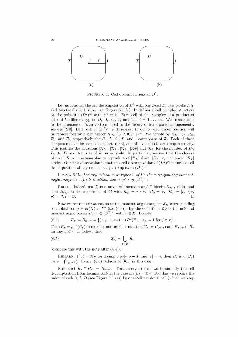
90 6. MOMENT-ANGLE COMPLEXES
'
&
$
%
s s0 1ITD
(a)
'
&
$
%
s1TD
(b)
Figure 6.1. Cell decompositions of D2.
Let us consider the cell decomposition of D2 with one 2-cell D, two 1-cells I, Tand two 0-cells 0, 1, shown on Figure 6.1 (a). It defines a cell complex structureon the poly-disc (D2)m with 5m cells. Each cell of this complex is a product ofcells of 5 different types: Di, Ii, 0i, Ti and 1i, i = 1, . . . , m. We encode cellsin the language of “sign vectors” used in the theory of hyperplane arrangements,see e.g. [22]. Each cell of (D2)m with respect to our 5m-cell decomposition willbe represented by a sign vector R ∈ D, I, 0, T, 1m. We denote by RD, RI , R0,RT and R1 respectively the D-, I-, 0-, T - and 1-component of R. Each of thesecomponents can be seen as a subset of [m], and all five subsets are complementary.This justifies the notations |RD|, |RI |, |R0|, |RT | and |R1| for the number of D-,I-, 0-, T - and 1-entries of R respectively. In particular, we see that the closureof a cell R is homeomorphic to a product of |RD| discs, |RI | segments and |RT |circles. Our first observation is that this cell decomposition of (D2)m induces a celldecomposition of any moment-angle complex in (D2)m:
Lemma 6.15. For any cubical subcomplex C of Im the corresponding moment-angle complex ma(C) is a cellular subcomplex of (D2)m.
Proof. Indeed, ma(C) is a union of “moment-angle” blocks Bσ⊂τ (6.2), andeach Bσ⊂τ is the closure of cell R with RD = τ \ σ, R0 = σ, RT = [m] \ τ ,RI = R1 = ∅. ¤
Now we restrict our attention to the moment-angle complex ZK correspondingto cubical complex cc(K) ⊂ Im (see (6.3)). By the definition, ZK is the union ofmoment-angle blocks Bσ⊂τ ⊂ (D2)m with τ ∈ K. Denote
(6.4) Bτ := B∅⊂τ =(z1, . . . , zm) ∈ (D2)m : |zj | = 1 for j /∈ τ
.
Then Bτ = ρ−1(Cτ ) (remember our previous notation Cτ := C∅⊂τ ) and Bσ⊂τ ⊂ Bτ
for any σ ⊂ τ . It follows that
(6.5) ZK =⋃
τ∈K
Bτ
(compare this with the note after (4.4)).
Remark. If K = KP for a simple polytope P and |τ | = n, then Bτ is ie(Bv)for v =
⋂j∈τ Fj . Hence, (6.5) reduces to (6.1) in this case.
Note that Bτ ∩ Bτ ′ = Bτ∩τ ′ . This observation allows to simplify the celldecomposition from Lemma 6.15 in the case ma(C) = ZK . For this we replace theunion of cells 0, I, D (see Figure 6.1 (a)) by one 2-dimensional cell (which we keep
6.3. CELL DECOMPOSITIONS OF MOMENT-ANGLE COMPLEXES 91
denoting D for simplicity). The resulting cell decomposition of D2 with 3 cells isshown on Figure 6.1 (b). It defines a cell decomposition of (D2)m with 3m cells,each of which is a product of 3 different types Di, Ti and 1i, i = 1, . . . , m. Againwe use the sign vector language and encode the new cells of (D2)m by sign vectorsT ∈ D, T, 1m. The notations TD, |TT | etc. have the same meaning as in the caseof 5m-cell decomposition. The closure of T is now a product of |TD| discs and |TT |circles.
Lemma 6.16. The moment-angle complex ZK is a cellular subcomplex of (D2)m
with respect to the 3m-cell decomposition (see Figure 6.1 (b)). Those cells T ⊂(D2)m which form ZK are determined by the condition TD ∈ K.
Proof. Since Bτ = B∅⊂τ is the closure of cell T with TD = τ , TT = [m] \ τand T1 = ∅, the statement follows from (6.5). ¤
Remark. Note that for general C the moment-angle complex ma(C) is not acell subcomplex with respect to the 3m-cell decomposition of (D2)m.
Lemma 6.17. Let φ : K1 → K2 be an inclusion of simplicial complexes onthe sets [m1] and [m2] respectively. Then it induces an equivariant cellular mapφma : ZK1 → ZK2 of the corresponding moment-angle complexes.
Proof. Assign the i-th vector of the standard basis of Cm1 to the elementi ∈ [m1], and similarly for Cm2 and [m2]. This allows to extend the map φ : [m1] →[m2] to an inclusion φC : Cm1 → Cm2 . For any subset τ ⊂ [m1] the map φC takesBτ ⊂ Cm1 (see (6.4)) to Bφ(τ) ⊂ Cm2 . Since φ is a simplicial map, for τ a simplexof K1 we have φ(τ) ∈ K2 and φC(Bτ ) ⊂ ZK2 (see (6.5)). Hence, φC defines an(equivariant) map φma : ZK1 → ZK2 . ¤
Let us apply the construction of ZK (see (6.3)) to the case when K = ∅(regarded as a simplicial complex on [m]). Then cc(K) = (1, . . . , 1) ∈ Im (the coneover the empty set is just one vertex), and so Z∅ = ρ−1(1, . . . , 1) ∼= Tm, whereZ∅ = Z∅,[m]. (Another way to see this is to apply Proposition 6.11 in the caseK = ∅.) We also observe that Z∅ is contained in ZK for any K on [m] as aTm-stable subset.
Lemma 6.18. Let K be a simplicial complex on the vertex set [m]. The inclusionZ∅ → ZK is a cellular embedding homotopical to a map to a point, i.e. the torusZ∅ is a cellular subcomplex contractible within ZK .
Proof. Z∅ ⊂ ZK is a cellular subcomplex since it is the closure of the m-dimensional cell T with TT = [m]. So it remains to prove that Tm is contractiblewithin ZK . We do this by induction on m. If m = 1 then the only option forK is K = ∆0 (0-simplex), so ZK = D2 (see Example 6.12.2) and Z∅,[1] = S1 iscontractible in ZK . Now suppose that the vertex set of K is [m]. The embeddingunder the question factors as
(6.6) Z∅,[m] → ZK[m−1],[m] → ZK,[m],
where K[m−1] is the maximal subcomplex of K on the vertex set [m− 1], see (2.1).By Proposition 6.11, Z∅,[m] = Z∅,[m−1] × S1 and ZK[m−1],[m] = ZK[m−1],[m−1] ×S1. By the inductive hypothesis we may assume that the embedding Z∅,[m−1] ⊂ZK[m−1],[m−1] is null-homotopic, so the composite embedding (6.6) is homotopic tothe map Z∅,[m−1] × S1 → ZK,[m] that sends Z∅,[m−1] to a point and S1 to the
92 6. MOMENT-ANGLE COMPLEXES
closure of the cell (1, . . . , 1, T ) ⊂ ZK,[m] (the latter is understood as a vector ofletters D, T, 1). But since m is a vertex of K, the complex ZK also contains thecell (1, . . . , 1, D), so a disc D2 is patched to the closure of (1, . . . , 1, T ). It followsthat the whole map (6.6) is null-homotopic. ¤
Corollary 6.19. For any simplicial complex K on the vertex set [m] themoment-angle complex ZK is simply connected.
Proof. Indeed, the 1-skeleton of our cellular decomposition of ZK is containedin the torus Z∅, which is null-homotopic by Lemma 6.18. ¤
6.4. Moment-angle complexes corresponding to joins, connected sumsand bistellar moves
Here we study the behavior of moment-angle complexes ZK with respect toconstructions from section 2.2. In particular, we describe moment-angle complexescorresponding to joins and connected sums of simplicial complexes and interpretbistellar moves (see Definition 2.39) as certain surgery-like operations on moment-angle complexes.
Agreement. Let τ = j1, . . . , jk be a subset of [m]. In this section we willdenote the moment-angle block Bτ
∼= (D2)k × Tm−k (6.4) by D2kτ × Tm−k. The
boundary of Bτ is
∂Bτ =⋃
j∈τ
D2k−2τ\j × Tm−k+1 ∼= S2k−1 × Tm−k
(compare with Example 6.7). We denote ∂Bτ = S2k−1τ × Tm−k. Furthermore, for
any partition [m] = σ∪τ ∪ρ into three complementary subsets with |σ| = i, |τ | = j,|ρ| = r, we will use the notation D2i
σ × S2j−1τ × T r
ρ for the corresponding subsetof (D2)m.
Construction 6.20 (moment-angle complex corresponding to join). Let K1,K2 be simplicial complexes on the sets [m1], [m2] respectively, and K1 ∗K2 the joinof K1 and K2 (see Construction 2.9). Identify the cube Im1+m2 with Im1 × Im2 .Then, using (4.4), we calculate
cc(K1 ∗K2) =⋃
τ1∈K1, τ2∈K2
Cτ1∪τ2 =⋃
τ1∈K1, τ2∈K2
Cτ1 × Cτ2
=( ⋃
τ1∈K1
Cτ1
)×
( ⋃
τ2∈K2
Cτ2
)= cc(K1)× cc(K2).
Hence,ZK1∗K2 = ZK1 ×ZK2 .
This can be thought as a generalization of Proposition 6.4 to arbitrary simplicialcomplexes.
Construction 6.21 (moment-angle complexes and connected sums). Supposewe are given two pure (n− 1)-dimensional simplicial complexes K1, K2 on the sets[m1], [m2] respectively, and let K1 # K2 be their connected sum at some σ1 andσ2. (Here K1 # K2 is considered as a simplicial complex on [m1 + m2 − n], withsuitable identification σ1 = σ2 = σ, see Construction 2.12). If we regard K1 as asimplicial complex on [m1+m2−n], then the corresponding moment-angle complex
6.4. JOINS, CONNECTED SUMS AND BISTELLAR MOVES 93
is ZK1 × Tm2−n (Proposition 6.11), where ZK1 = ZK1,[m1], and similarly for K2.Denote K1 := K1 \ σ1 and K2 := K2 \ σ2. Then
(6.7) Z bK1= ZK1 \ (Tm1−n ×D2n
σ1), Z bK2
= ZK2 \ (D2nσ2× Tm2−n)
by (6.5). Now we see that
(6.8) ZK1#K2 = Z bK1× Tm2−n ∪ Tm1−n ×Z bK2
,
where the two pieces are glued along Tm1−n×S2n−1σ1
×Tm2−n ∼= Tm1−n×S2n−1σ2
×Tm2−n, using the identification of σ1 with σ2. Equivalently,
ZK1#K2 =⋃
τ∈K1 or τ∈K2τ 6=σ
D2|τ |τ × Tm1+m2−n−|τ |.
Example 6.22. Let K1 = K be a pure (n− 1)-dimensional simplicial complexon [m] and K2 = ∂∆n (the boundary of n-simplex). Choose a maximal simplexσ ∈ K and consider the connected sum K #σ ∂∆n (the choice of a maximal simplexin ∂∆n is irrelevant). Note that Z∂∆n ∼= S2n+1 can be decomposed as
D2nσ × S1 ∪S2n−1×S1 S2n−1
σ ×D2
(see examples 6.7 and 6.12), therefore Zd∂∆n = S2n−1σ ×D2. Now it follows from (6.8)
and (6.7) that
(6.9) ZK#σ∂∆n
=(ZK × S1 \ Tm−n ×D2n
σ × S1) ∪T m−n×S2n−1×S1 (Tm−n × S2n−1
σ ×D2).
Thus, ZK#σ∂∆n is obtained by removing the “equivariant” handle Tm−n ×D2n ×S1 from ZK × S1 and then attaching Tm−n × S2n−1 × D2 along the boundaryTm−n × S2n−1 × S1.
As we mentioned above, the connected sum with the boundary of simplex isa bistellar 0-move. Other bistellar moves also can be interpreted as “equivariantsurgery operations” on ZK .
Construction 6.23 (equivariant surgery operations). Let K be an (n − 1)-dimensional pure simplicial complex on [m], and let σ ∈ K be an (n−1−k)-simplex(1 ≤ k ≤ n− 2) such that link σ is the boundary ∂τ of a k-simplex τ that is not aface of K. Let K ′ be the complex obtained from K by applying the correspondingbistellar k-move, see Definition 2.39:
(6.10) K ′ =(K \ (σ ∗ ∂τ)
) ∪ (∂σ ∗ τ)
(note that due to our assumptions K ′ has the same number of vertices as K).The moment-angle complexes corresponding to σ ∗ ∂τ and ∂σ ∗ τ are D
2(n−k)σ ×
S2k+1τ and S
2(n−k)−1σ × D
2(k+1)τ respectively (this follows from Example 6.12 and
Construction 6.20). Using stabilization arguments (Proposition 6.11), we obtain
(6.11) ZK′ =(ZK\Tm−n−1×D2(n−k)
σ ×S2k+1τ
)∪(Tm−n−1×S2(n−k)−1σ ×D2(k+1)
τ ),
where Tm−n−1 × S2(n−k)−1σ × D
2(k+1)τ is attached along its boundary Tm−n−1 ×
S2(n−k)−1×S2k+1. This describes the behavior of ZK under bistellar k-moves (thecases k = 0 and k = n− 1 are covered by (6.9)).
94 6. MOMENT-ANGLE COMPLEXES
Lemma 6.24. Let K = Kn−1 be a simplicial sphere and K ′ the simplicialsphere obtained from K by applying a bistellar k-move (6.10), 0 < k < n − 1.Then the corresponding moment-angle manifolds ZK and Z ′K are Tm-equivariantlycobordant. If K ′ is obtained from K by applying a 0-move, then ZK′ is cobordantto ZK × S1.
Proof. We give a proof for k-moves, k > 1. The case k = 0 is consideredsimilarly. Consider the product U = ZK × [0, 1] of ZK with a segment. DefineX = Tm−n−1×D
2(n−k)σ ×S2k+1
τ and Y = Tm−n−1×D2(n−k)σ ×D
2(k+1)τ (the latter
is a “solid equivariant handle”). Since X ⊂ ZK and X ⊂ ∂Y , we can attach Y toU at X × 1 ⊂ ZK × 1. Denote the resulting manifold (with boundary) by V , i.e.V = U ∪X Y . Then it follows from (6.11) that ∂V = ZK ∪ ZK′ (here ZK comesfrom ZK × 0 ⊂ U , while ZK × 1 is replaced by ZK′). This concludes the proof. ¤
Now we have the following topological corollary of Pachner’s Theorem 2.40.
Theorem 6.25. Let Kn−1 be a PL sphere. Then for some p the moment-anglemanifold ZK×T p is equivariantly cobordant to S2n+1×Tm+p−n−1. This cobordismis realized by a sequence of equivariant surgeries.
Proof. By Theorem 2.40, the PL sphere K is taken to ∂∆n by a sequence ofbistellar moves. Since Z∂∆n ∼= S2n+1, the statement follows from Lemma 6.24. ¤
6.5. Borel constructions and Davis–Januszkiewicz space
Here we study basic homotopy properties of ZK . We also provide necessaryarguments for the statements about the cohomology of quasitoric manifolds, whichwe left unproved in section 5.2.
Let ETm be the contractible space of the universal principal Tm-bundle overclassifying space BTm. It is well known that BTm is (homotopy equivalent to) theproduct of m copies of infinite-dimensional projective space CP∞. The cell decom-position of CP∞ with one cell in every even dimension determines the canonicalcell decomposition of BTm. The cohomology of BTm (with coefficients in k) isthus the polynomial ring k[v1, . . . , vm], deg vi = 2.
Definition 6.26. Let X be a Tm-space. The Borel construction (alternatively,homotopy quotient or associated bundle) is the identification space
ETm ×T m X := ETm ×X/∼,
where (e, x) ∼ (eg, g−1x) for any e ∈ ETm, x ∈ X, g ∈ Tm.
The projection (e, x) → e displays ETm ×T m X as the total space of a bundleETm ×T m X → BTm with fibre X and structure group Tm. At the same time,there is a principal Tm-bundle ETm ×X → ETm ×T m X.
In the sequel we denote the Borel construction ETm ×T m X corresponding toa Tm-space X by BT X. In particular, for any simplicial complex K on m verticeswe have the Borel construction BTZK and the bundle p : BTZK → BTm withfibre ZK .
For each i = 1, . . . ,m denote by BTi the i-th factor in BTm = (CP∞)m. Fora subset σ ⊂ [m] we denote by BTσ the product of BTi’s with i ∈ σ. Obviously,BTσ is a cellular subcomplex of BTm, and BTσ
∼= BT k if |σ| = k.
6.5. BOREL CONSTRUCTIONS AND DAVIS–JANUSZKIEWICZ SPACE 95
Definition 6.27. Let K be a simplicial complex. We refer to the cellularsubcomplex ⋃
σ∈K
BTσ ⊂ BTm
as the Davis–Januszkiewicz space, and denote it DJ (K).
The name is justified by the following statement, which is an immediate corollaryof the definition of Stanley–Reisner ring k(K) (Definition 3.1).
Proposition 6.28. The cellular cochain algebra C∗(DJ (K)) and the cohomol-ogy algebra H∗(DJ (K)) are isomorphic to the face ring k(K). The cellular inclusioni : DJ (K) → BTm induces the quotient epimorphism i∗ : k[v1, . . . , vm] → k(K) =k[v1, . . . , vm]/IK in the cohomology.
Theorem 6.29. The fibration p : BTZK → BTm is homotopy equivalent tothe cellular inclusion i : DJ (K) → BTm. More precisely, there is a deformationretraction BTZK → DJ (K) such that the diagram
BTZKp−−−−→ BTm
y∥∥∥
DJ (K) i−−−−→ BTm
is commutative.
Proof. Consider the decomposition (6.5). Since each Bτ ⊂ ZK is Tm-stable,the Borel construction BTZK = ETm×T m ZK is patched from the Borel construc-tions ETm×T m Bτ for τ ∈ K. Suppose |τ | = j; then Bτ
∼= (D2)j×Tm−j (see (6.4)).By the definition of Borel construction, ETm×T m Bτ
∼= (ET j×T j (D2)j)×ETm−j .The space ET j ×T j (D2)j is the total space of a (D2)j-bundle over BT j . It followsthat there is a deformation retraction ETm×T m Bτ → BTτ , which defines a homo-topy equivalence between the restriction of p : BTZK → BTm to ETm×T m Bτ andthe cellular inclusion BTτ → BTm. These homotopy equivalences correspondingto different simplices τ ∈ K fit together to yield a required homotopy equivalencebetween p : BTZK → BTm and i : DJ (K) → BTm. ¤
Corollary 6.30. The moment-angle complex ZK is the homotopy fibre of thecellular inclusion i : DJ (K) → BTm.
As a corollary, we get the following statement, firstly proved in [48, Theo-rem 4.8].
Corollary 6.31. The cohomology algebra H∗(BTZK) is isomorphic to theface ring k(K). The projection p : BTZK → BTm induces the quotient epimor-phism p∗ : k[v1, . . . , vm] → k(K) = k[v1, . . . , vm]/IK in the cohomology.
Corollary 6.32. The Tm-equivariant cohomology of ZK is isomorphic to theStanley–Reisner ring of K:
H∗T m(ZK) ∼= k(K).
The following information about the homotopy groups of ZK can be retrievedfrom the above constructions.
96 6. MOMENT-ANGLE COMPLEXES
Theorem 6.33. (a) The complex ZK is 2-connected (i.e. π1(ZK) = π2(ZK) =0), and πi(ZK) = πi(BTZK) = πi(DJ (K)) for i ≥ 3.
(b) If K = KP and P is q-neighborly (see Definition 1.15), then πi(ZK) = 0for i < 2q + 1. Moreover, π2q+1(ZP ) is a free Abelian group generated by the(q + 1)-element missing faces of KP .
Proof. Note that BTm = K(Zm, 2) and the 3-skeleton of DJ (K) coincideswith that of BTm. If P is q-neighborly, then it follows from Definition 6.27 that the(2q + 1)-skeleton of DJ (KP ) coincides with that of BTm. Now, both statementsfollow easily from the exact homotopy sequence of the map i : DJ (K) → BTm withhomotopy fibre ZK (see Corollary 6.30). ¤
Remark. Say that a simplicial complex K on the set [m] is k-neighborly if anyk-element subset of [m] is a simplex of K. (This definition is an obvious extensionof the notion of k-neighborly simplicial polytope to arbitrary simplicial complexes).Then the second part of Theorem 6.33 holds for arbitrary q-neighborly simplicialcomplex.
Suppose now that K = KP for some simple n-polytope P and M2n is a qua-sitoric manifold over P with characteristic function ` (see Definition 5.10). Then wehave the subgroup H(`) ⊂ Tm acting freely on ZP and the principal Tm−n-bundleZP → M2n (Proposition 6.5).
Proposition 6.34. The Borel construction ETn ×T n M2n is homotopy equiv-alent to BTZP .
Proof. Since H(`) acts freely on ZP , we have
BTZP = ETm ×T m ZP
∼= EH(`)×(E
(Tm/H(`)
)×T m/H(`) ZP /H(`))' ETn ×T n M2n.
¤
Corollary 6.35. The Tn-equivariant cohomology ring of a quasitoric manifoldM2n over Pn is isomorphic to the Stanley–Reisner ring of Pn:
H∗T n(M2n) ∼= k(Pn).
Proof. It follows from Proposition 6.34 and Corollary 6.32. ¤
Theorem 6.36 ([48, Theorem 4.12]). The Leray–Serre spectral sequence of thebundle
(6.12) ETn ×T n M2n → BTn
with fibre M2n collapses at the E2 term, i.e. Ep,q2 = Ep,q
∞ .
Proof. Since both BTn and M2n have only even-dimensional cells (see Propo-sition 5.16), all the differentials in the spectral sequence are trivial by dimensionalreasons. ¤
Corollary 6.37. Projection (6.12) induces a monomorphism k[t1, . . . , tn] →k(P ) in the cohomology. The inclusion of fibre M2n → ETn ×T n M2n induces anepimorphism k(P ) → H∗(M2n).
Now we are ready to give proofs for the statements from section 5.2.
6.6. WALK AROUND THE CONSTRUCTION OF ZK 97
Proof of Lemma 5.17 and Theorem 5.18. The monomorphism
H∗(BTn) = k[t1, . . . , tn] → k(P ) = H∗(ETn ×T n M2n)
takes ti to θi, i = 1, . . . , n. By Theorem 6.36, k(P ) is a free k[t1, . . . , tn]-module,hence, θ1, . . . , θn is a regular sequence. Therefore, the kernel of k(P ) → H∗(M2n)is exactly J` = (θ1, . . . , θn). ¤
6.6. Walk around the construction of ZK : generalizations, analoguesand additional comments
Many our previous constructions (namely, the cubical complex cc(K), themoment-angle complex ZK , the Borel construction BTZK , the Davis–Januszkiewiczspace DJ (K), and also the complement U(K) of a coordinate subspace arrange-ment appearing in section 8.2) admit a unifying combinatorial interpretation interms of the following construction, which was mentioned to us by N. Strickland(in private communications).
Construction 6.38. Let X be a space, and W a subspace of X. Let K be asimplicial complex on the set [m]. Define the following subset in the product of mcopies of X:
K•(X, W ) =⋃
σ∈K
(∏
i∈σ
X ×∏
i/∈σ
W).
Example 6.39. 1. cc(K) = K•(I1, 1) (see (4.4)).2. ZK = K•(D2, S1) (see (6.5)).3. DJ (K) = K•(CP∞, ∗) (see Definition 6.27).4. BTZK = K•(ES1 ×S1 D2, ES1 ×S1 S1) (see the proof of Theorem 6.29).
Another unifying description of the above spaces can be achieved using categor-ical constructions of limits and colimits of different diagrams over the face categorycat(K) of K. (The objects of cat(K) are simplices σ ∈ K and the morphismsare inclusions.) For instance, Definition 6.27 is an example of this procedure: theDavis–Januszkiewicz space is the colimit of the diagram of spaces over cat(K) thatassigns BTσ to a simplex σ ∈ K. In the case when K is a flag complex (see Def-inition 2.18 and Proposition 2.19) the colimit over cat(K) reduces to the graphproduct , studied in the theory of groups (see e.g. [43]). Well-known examples ofgraph products include right-angled Coxeter and Artin groups (see e.g. [48], [49]).The most general categorical setup for the above constructions involves the notionof homotopy colimit [24], [138]. This fundamental algebraic-topological concepthas already found combinatorial applications, see [139]. The complex ZK can beseen as the homotopy colimit of a certain diagram of tori; this interpretation issimilar to the homotopy colimit description of toric varieties proposed in [139].For more information on this approach see [113].
The combinatorial theory of toric spaces is parallel to some extent to its Z/2-,or “real”, counterpart. We say a few words about the Z/2-theory here, referringthe reader to [48], [49] and other papers of R. Charney, M. Davis, T. Januszkiewiczand their co-authors for more detailed treatment (some further results can be alsofound in [113]). The first step is to pass from the torus Tm to its “real analogue”,the group (Z/2)m. The standard cube Im = [0, 1]m is the orbit space for theaction of (Z/2)m on the bigger cube [−1, 1]m, which in turn can be regarded as a“real analogue” of the poly-disc (D2)m ⊂ Cm. Now, given a cubical subcomplex
98 6. MOMENT-ANGLE COMPLEXES
C ⊂ Im, one can construct a (Z/2)m-symmetrical cubical complex embedded into[−1, 1]m just in the same way as it is done in Definition 6.10. In particular, for anysimplicial complex K on the vertex set [m] one can introduce the real versions RZK
and RWK of the moment-angle complexes ZK and WK (6.3). In the notations ofConstruction 6.38 we have
RZK = K•([−1, 1], −1, 1).
This cubical complex was studied, e.g. in [10] under the name mirroring construc-tion. If K is a simplicial (n−1)-sphere, then RZK is an n-dimensional manifold (theproof is similar to that of Lemma 6.13). Thereby, for any simplicial sphere Kn−1
with m vertices we get a (Z/2)m-symmetric n-manifold with a (Z/2)m-invariant cu-bical subdivision. As suggested by the results of [10], this class of cubical manifoldsmay be useful in the combinatorial theory of face vectors of cubical complexes (seesection 4.1). The real analogue RZP of the manifold ZP (corresponding to the caseof a polytopal simplicial sphere) is the universal Abelian cover of the polytope Pn
regarded as an orbifold (or manifold with corners), see e.g. [68, §4.5]. In [78] man-ifolds RZP and ZP are interpreted as the configuration spaces of equivariant hingemechanisms (or linkages) in R2 and R3.
Example 6.40. Let P 2m be an m-gon. Then RZP 2
mis a 2-dimensional manifold.
It is easy to see that RZP 23
= RZ∆2 ∼= S2 (a 2-sphere patched from 8 triangles)and RZP 2
4= RZ∆1×∆1 ∼= T 2 (a 2-torus patched from 16 squares). More generally,
RZP 2m
is patched from 2m polygons, meeting by 4 at each vertex. Hence, we havem2m−2 vertices and m2m−1 edges, so the Euler characteristic is
χ(RZP 2m
) = 2m−2(4−m).
Thus, RZP 2m
is a surface of genus 1−2m−1 +m2m−3. This also can be seen directlyby decomposing P 2
m into a connected sum of an (m−1)-gon and triangle and usingthe real version of Example 6.22.
Replacing Tn by (Z/2)n in Definition 5.10, we obtain a real version of quasitoricmanifolds, which was introduced in [48] under the name small covers. Thereby asmall cover of a simple polytope Pn is a (Z/2)n-manifold Mn with quotient Pn. Thename refers to the fact that any branched cover of Pn (as an orbifold) by a smoothmanifold have at least 2n sheets. Small covers were studied in [48] along withquasitoric manifolds, and many results on quasitoric manifolds quoted from [48]in section 5.2 have analogues in the small cover case. Also, like in the torus case,every small cover is the quotient of the universal cover RZP by a free action of thegroup (Z/2)m−n.
An important class of small covers (and quasitoric manifolds) was introducedin [48, Example 1.15] under the name pullbacks from the linear model . They cor-respond to simple polytopes Pn whose dual triangulation can be folded onto the(n− 1)-simplex (more precisely, the polytopal sphere KP admits a non-degeneratesimplicial map onto ∆n−1; note that this is always the case when KP is a barycen-tric subdivision of some other polytopal sphere, see Example 2.15). If this conditionis satisfied then there exists a special characteristic map (5.4) which assigns to eachfacet of Pn a coordinate subtorus Ti ⊂ Tn (or coordinate subgroup (Z/2)i ⊂ (Z/2)n
in the small cover case). Pullbacks from the linear model have a number of niceproperties, in particular, they are all stably parallelizable ([48, Corollary 6.10],compare with Theorem 5.33). The existence of a non-degenerate simplicial map
6.6. WALK AROUND THE CONSTRUCTION OF ZK 99
from KP to ∆n−1 can be reformulated by saying that the polytope Pn admits aregular n-paint coloring . The latter means that the facets of Pn can be coloredwith n paints in such a way that any two adjacent facets have different color. Asimple polytope Pn admits a regular n-paint coloring if and only if every its 2-facehas an even number of edges. This is a classical result for n = 3; the proof in thegeneral case can be found in [81]. Some additional results about pullbacks fromthe linear model in dimension 3 were obtained in [79]. It was shown there that anysmall cover M3 which is a pullback from the linear model admits an equivariantembedding into R4 = R3 × R with the standard action of (Z/2)3 on R3 and thetrivial action on R. Another result from [79] says that any such M3 can be ob-tained from a set of 3-dimensional tori by applying several equivariant connectedsums and equivariant Dehn twists (compare with section 6.4).
Although not any simple 3-polytope admits a regular 3-paint coloring, a regular4-paint coloring can always be achieved due to the Four Color Theorem. Thisargument was used in [48, Example 1.21] to prove that there is a small cover(or quasitoric manifold) over every simple 3-polytope. (One can just construct acharacteristic map by assigning the coordinate circles in T 3 to first three colors andthe diagonal circle to the fourth one).
On the other hand, it would be particularly interesting to develop a quaternionicanalogue of the theory. Unlike the real case, not much is done here. For start, ofcourse, we have to replace Tn by the quaternionic torus Sp(1)n ∼= (S3)n. Developingquaternionic analogues of toric and quasitoric manifolds is quite tricky. R. Scottin [119] used the quaternionic analogue of characteristic map to approach thisproblem. However, the non-commutativity of the quaternionic torus implies thatit does not contain sufficiently many subgroups for the resulting quaternionic toricmanifolds to have an actual Sp(1)n-action. A polytopal structure also appears in thequotients of some other types of manifolds studied in the quaternionic geometry, seee.g. [25]. We also mention that since only coordinate subgroups of Tm are involvedin the definition of the moment-angle complex ZK , this particular construction ofa toric space does have a quaternionic analogue which is an Sp(1)m-space.
At the end we give one example which builds on a generalization of the con-struction of ZK to the case of an arbitrary group G.
Example 6.41 (classifying space for group G). Let K be a simplicial complexon the vertex set [m]. Set ZK(G) := K•(cone(G), G) (see Construction 6.38), wherecone(G) is the cone over G with the obvious G-action. By the construction, thegroup Gm acts on ZK(G), with quotient cone(K). It is also easy to observe thatthe diagonal subgroup in Gm acts freely on ZK(G), thus identifying ZK(G) as aprincipal G-space.
Suppose now that K1 ⊂ K2 ⊂ · · · ⊂ Ki ⊂ · · · is a sequence of embeddedsimplicial complexes such that Ki is i-neighborly. The group G acts freely on thecontractible space lim
−→ZKi(G), and the corresponding quotient is thus the classifying
space BG. Thus, we have the following filtration in the universal fibration EG →BG:
ZK1(G) → ZK2(G) → · · · → ZKi(G) → · · ·↓ ↓ ↓
ZK1(G)/G → ZK2(G)/G → · · · → ZKi(G)/G → · · · .
100 6. MOMENT-ANGLE COMPLEXES
The well-known Milnor filtration in the universal fibration of the group G corre-sponds to the case Ki = ∆i−1.
CHAPTER 7
Cohomology of moment-angle complexes andcombinatorics of triangulated manifolds
7.1. The Eilenberg–Moore spectral sequence
In their paper [60] of 1966, Eilenberg and Moore constructed a spectral se-quence of great importance for algebraic topology. This spectral sequence can beconsidered as an extension of Adams’ approach to calculating the cohomology ofloop spaces [1]. In 1960-70s different applications of the Eilenberg–Moore spec-tral sequence led to many important results on the cohomology of loop spaces andhomogeneous spaces for Lie group actions. In this chapter we discuss some newapplications of this spectral sequence to combinatorial problems. This section con-tains the necessary information about the spectral sequence; we follow L. Smith’spaper [121] in this description.
The following theorem provides an algebraic setup for the Eilenberg–Moorespectral sequence.
Theorem 7.1 (Eilenberg–Moore [121, Theorem 1.2]). Let A be a commutativedifferential graded k-algebra, and M , N differential graded A-modules. Then thereexists a spectral sequence Er, dr converging to TorA(M, N) and whose E2-termis
E−i,j2 = Tor−i,j
H[A]
(H[M ], H[N ]
), i, j ≥ 0,
where H[·] denotes the cohomology algebra (or module).
The above spectral sequence lives in the second quadrant and its differentialsdr add (r, 1 − r) to bidegree, r ≥ 1. It is called the (algebraic) Eilenberg–Moorespectral sequence. For the corresponding decreasing filtration F−p TorA(M, N)in TorA(M, N) we have
E−p,n+p∞ = F−p
( ∑
−i+j=n
Tor−i,jA (M,N)
)/F−p+1
( ∑
−i+j=n
Tor−i,jA (M, N)
).
Topological applications of Theorem 7.1 arise in the case when A,M, N aresingular (or cellular) cochain algebras of certain topological spaces. The classicalsituation is described by the commutative diagram
(7.1)
E −−−−→ E0yy
B −−−−→ B0,
where E0 → B0 is a Serre fibre bundle with fibre F over a simply connected base B0,and E → B is the pullback along a continuous map B → B0. For any space X, letC∗(X) denote either the singular cochain algebra of X or (in the case when X is a
101
102 7. COHOMOLOGY OF MOMENT-ANGLE COMPLEXES
cellular complex) the cellular cochain algebra of X. Obviously, C∗(E0) and C∗(B)are C∗(B0)-modules. Under these assumptions the following statement holds.
Lemma 7.2 ([121, Proposition 3.4]). TorC∗(B0)(C∗(E0), C∗(B)) is an algebra
in a natural way, and there is a canonical isomorphism of algebras
TorC∗(B0)
(C∗(E0), C∗(B)
) → H∗(E).
Applying Theorem 7.1 in the case A = C∗(B0), M = C∗(E0), N = C∗(B) andtaking into account Lemma 7.2, we come to the following statement.
Theorem 7.3 (Eilenberg–Moore). There exists a spectral sequence of commu-tative algebras Er, dr with
(a) Er ⇒ H∗(E);(b) E−i,j
2 = Tor−i,jH∗(B0)
(H∗(E0), H∗(B)
).
The spectral sequence of Theorem 7.3 is called the (topological) Eilenberg–Moore spectral sequence. The case when B in (7.1) is a point is particularly impor-tant for applications, so we state the corresponding result separately.
Corollary 7.4. Let E → B be a fibration over a simply connected space Bwith fibre F . Then there exists a spectral sequence of commutative algebras Er, drwith
(a) Er ⇒ H∗(F );(b) E2 = TorH∗(B)
(H∗(E),k
).
We refer to the spectral sequence of Corollary 7.3 as the Eilenberg–Moore spec-tral sequence of fibration E → B.
Example 7.5. Let M2n be a quasitoric manifold over Pn (see Definition 5.10).Consider the Eilenberg–Moore spectral sequence of the bundle ETn ×T n M2n →BTn with fibre M2n. By Proposition 6.34, H∗(ETn ×T n M2n) = H∗(BTZP ) ∼=k(Pn). The monomorphism
k[t1, . . . , tn] = H∗(BTn) → H∗(ETn ×T n M2n) = k(Pn)
takes ti to θi (i = 1, . . . , n), see (5.6). The E2 term of the Eilenberg–Moore spectralsequence is
E∗,∗2 = Tor∗,∗H∗(BT n)
(H∗(ETn ×T n M2n),k
)= Tor∗,∗k[t1,...,tn]
(k(Pn),k
).
Since k(Pn) is a free k[t1, . . . , tn]-module, we have
Tor∗,∗k[t1,...,tn]
(k(Pn),k
)= Tor0,∗
k[t1,...,tn]
(k(Pn),k
)
= k(Pn)⊗k[t1,...,tn] k = k(Pn)/(θ1, . . . , θn).
Therefore, E0,∗2 = k(Pn)/J` and E−p,∗
2 = 0 for p > 0. It follows that the Eilenberg–Moore spectral sequence collapses at the E2 term and H∗(M2n) = k(Pn)/J`, inaccordance with Theorem 5.18.
7.2. Cohomology algebra of ZK
Here we apply the Eilenberg–Moore spectral sequence to calculating the coho-mology algebra of the moment-angle complex ZK . As an immediate corollary weobtain that the cohomology algebra inherits a canonical bigrading from the spec-tral sequence. The corresponding bigraded Betti numbers coincide with importantcombinatorial invariants of K introduced by Stanley [128].
7.2. COHOMOLOGY ALGEBRA OF ZK 103
Theorem 7.6. The following isomorphism of algebras holds:
H∗(ZK) ∼= Tork[v1,...,vm]
(k(K),k
).
This formula either can be seen as an isomorphism of graded algebras, where thegrading in the right hand side is by the total degree, or used to define a bigradedalgebra structure in the left hand side. In particular,
Hp(ZK) ∼=∑
−i+2j=p
Tor−i,2jk[v1,...,vm]
(k(K),k
).
Proof. Let us consider the Eilenberg–Moore spectral sequence of the commu-tative square
(7.2)
E −−−−→ ETm
yy
DJ (K) i−−−−→ BTm,
where the left vertical arrow is the pullback along i. Corollary 6.30 shows that Eis homotopy equivalent to ZK .
By Proposition 6.28, the map i : DJ (K) → BTm induces the quotient epimor-phism
i∗ : C∗(BTm) = k[v1, . . . , vm] → k(K) = C∗(DJ (K)),
where C∗(·) denotes the cellular cochain algebra. Since ETm is contractible, thereis a chain equivalence C∗(ETm) ' k. More precisely, C∗(ETm) can be identifiedwith the Koszul resolution Λ[u1, . . . , um] ⊗ k[v1, . . . , vm] of k (see Example 3.24).Therefore, we have an isomorphism
(7.3) TorC∗(BT m)
(C∗
(DJ (K)
), C∗(ETm)
) ∼= Tork[v1,...,vm]
(k(K),k
).
The Eilenberg–Moore spectral sequence of commutative square (7.2) has
E2 = TorH∗(BT m)
(H∗(DJ (K)
), H∗(ETm)
)
and converges to TorC∗(BT m)(C∗(DJ (K)), C∗(ETm)) (Theorem 7.1). Since
TorH∗(BT m)
(H∗(DJ (K)
),H∗(ETm)
)= Tork[v1,...,vm]
(k(K),k
),
it follows from (7.3) that the spectral sequence collapses at the E2 term, that is,E2 = E∞. Lemma 7.2 shows that the module TorC∗(BT m)(C∗(DJ (K)), C∗(ETm))is an algebra isomorphic to H∗(ZK), which concludes the proof. ¤
Theorem 7.6 displays the cohomology of ZK as a bigraded algebra and says thatthe corresponding bigraded Betti numbers b−i,2j(ZK) coincide with that of k(K),see (3.5). The next theorem follows from Lemma 3.29 and Corollary 3.30.
Theorem 7.7. The following isomorphism of bigraded algebras holds:
H∗,∗(ZK) ∼= H[Λ[u1, . . . , um]⊗ k(K), d
],
where the bigraded structure and the differential in the right hand side are definedby (3.4).
104 7. COHOMOLOGY OF MOMENT-ANGLE COMPLEXES
In the sequel, given two subsets σ = i1, . . . , ip, τ = j1, . . . , jq of [m], wewill denote the square-free monomial
ui1 . . . uipvj1 . . . vjq ∈ Λ[u1, . . . , um]⊗ k(K)
by uσvτ . Note that bideg uσvτ = (−p, 2(p + q)).
Remark. Since the differential d in (3.4) does not change the second degree,the differential bigraded algebra [Λ[u1, . . . , um] ⊗ k(K), d] splits into the sum ofdifferential subalgebras consisting of elements of fixed second degree.
Corollary 7.8. The Leray–Serre spectral sequence of the principal Tm-bundleETm ×ZK → BTZK collapses at the E3 term.
Proof. The spectral sequence under consideration converges to H∗(ETm ×ZK) = H∗(ZK) and has
E2 = H∗(Tm)⊗H∗(BTZK) = Λ[u1, . . . , um]⊗ k(K).
The differential in the E2 term acts as in (3.4). Hence,
E3 = H[E2, d] = H[Λ[u1, . . . , um]⊗ k(K)
]= H∗(ZK),
by Theorem 7.7. ¤
Construction 7.9. Consider the subspace A−q(K) ⊂ Λ[u1, . . . , um] ⊗ k(K)spanned by monomials uσ and uσvτ such that τ is a simplex of K, |σ| = q andσ ∩ τ = ∅. Define
A∗(K) =m⊕
q=0
A−q(K).
Since d(ui) = vi and d(vi) = 0, we have d(A−q(K)) ⊂ A−q+1(K). Therefore, A∗(K)is a cochain subcomplex in [Λ[u1, . . . , um]⊗k(K), d]. Moreover, A∗(K) inherits thebigraded module structure from Λ[u1, . . . , um] ⊗ k(K), with differential d adding(1, 0) to bidegree. Hence, we have an additive inclusion (i.e. a monomorphism ofbigraded modules) ia : A∗(K) → Λ[u1, . . . , um]⊗k(K). On the other hand, A∗(K)is an algebra in the obvious way, but is not a subalgebra of Λ[u1, . . . , um]⊗ k(K).(For instance, v2
1 = 0 in A∗(K), but v21 6= 0 in Λ[u1, . . . , um] ⊗ k(K).) Never-
theless, we have multiplicative projection (an epimorphism of bigraded algebras)jm : Λ[u1, . . . , um]⊗ k(K) → A∗(K). The additive inclusion ia and the multiplica-tive projection jm satisfy jm · ia = id.
Lemma 7.10. The cochain complexes [Λ[u1, . . . , um]⊗ k(K), d] and [A∗(K), d]are cochain homotopy equivalent and therefore have the same cohomology. Thisimplies the following isomorphism of bigraded k-modules:
H[A∗(K), d] ∼= Tork[v1,...,vm]
(k(K),k
).
Proof. A routine check shows that the cochain homotopy operator s forthe Koszul resolution (see the proof of Proposition VII.2.1 in [92]) establishes acochain homotopy equivalence between the maps id and ia · jm from the algebra[Λ[u1, . . . , um]⊗ k(K), d] to itself. That is,
ds + sd = id− ia · jm.
7.2. COHOMOLOGY ALGEBRA OF ZK 105
We just illustrate the above identity on few simple examples.
1) s(u1v2) = u1u2, ds(u1v2) = u2v1 − u1v2, sd(u1v2) = u1v2 − u2v1,
hence, (ds + sd)(u1v2) = 0 = (id− ia · jm)(u1v2);
2) s(u1v1) = u21 = 0, ds(u1v1) = 0, d(u1v1) = v2
1 , sd(u1v1) = u1v1,
hence, (ds + sd)(u1v1) = u1v1 = (id− ia · jm)(u1v1);
3) s(v21) = u1v1, ds(v2
1) = v21 , d(v2
1) = 0,
hence, (ds + sd)(v21) = v2
1 = (id− ia · jm)(v21).
¤Now we recall our cell decomposition of ZK , see Lemma 6.16. The cells of
ZK are the sign vectors T ∈ D, T, 1m with TD ∈ K. Assign to each pair σ, τ ofdisjoint subsets of [m] the vector T (σ, τ) with T (σ, τ)D = σ, T (σ, τ)T = τ . ThenT (σ, τ) is a cell of ZK if and only if σ ∈ K. Let C∗(ZK) and C∗(ZK) denote thecellular chain and cochain complexes of ZK respectively. Both complexes C∗(ZK)and A∗(K) have the same cohomology H∗(ZK). The complex C∗(ZK) has thecanonical additive basis consisting of cochains T (σ, τ)∗. As an algebra, C∗(ZK) isgenerated by the cochains D∗
i , T ∗j (of dimension 2 and 1 respectively) dual to thecells Di = T (i,∅) and Tj = T (∅, j), 1 ≤ i, j ≤ m. At the same time, A∗(K)is multiplicatively generated by vi, uj , 1 ≤ i, j ≤ m.
Theorem 7.11. The correspondence vσuτ 7→ T (σ, τ)∗ establishes a canonicalisomorphism between the differential graded algebras A∗(K) and C∗(ZK).
Proof. It follows directly from the definitions of A∗(K) and C∗(ZK) that theproposed map is an isomorphism of graded algebras. So it remains to prove thatit commutes with differentials. Let d, dc and ∂c denotes the differential in A∗(K),C∗(ZK) and C∗(ZK) respectively. Since d(vi) = 0 and d(ui) = vi, we need to showthat dc(D∗
i ) = 0, dc(T ∗i ) = D∗i . We have ∂c(Di) = Ti, ∂c(Ti) = 0. A 2-cell of ZK
is either Dj or Tjk = Tj × Tk (k 6= j). Then
〈dcT∗i , Dj〉 = 〈T ∗i , ∂cDj〉 = 〈T ∗i , Tj〉 = δij , 〈dcT
∗i , Tjk〉 = 〈T ∗i , ∂cTjk〉 = 0,
where δij = 1 if i = j and δij = 0 otherwise. Hence, dc(T ∗i ) = D∗i . Further, a 3-cell
of ZK is either DjTk or Tj1j2j3 = Tj1 × Tj2 × Tj3 . Then
〈dcD∗i , DjTk〉 = 〈D∗
i , ∂c(DjTk)〉 = 〈D∗i , Tjk〉 = 0,
〈dcD∗i , Tj1j2j3〉 = 〈D∗
i , ∂cTj1j2j3〉 = 0.
Hence, dc(D∗i ) = 0. ¤
The above theorem provides a topological interpretation for the differentialalgebra [A∗(K), d]. In the sequel we will not distinguish the cochain complexesA∗(K) and C∗(ZK), and identify ui with T ∗i , vi with D∗
i .Now we can summarise the results of Proposition 3.4, Lemma 3.32, Lemma 6.17,
Corollary 6.32 and Theorem 7.11 in the following statement describing the functorialproperties of the correspondence K 7→ ZK .
Proposition 7.12. Let us introduce the following functors:• Z, the covariant functor K 7→ ZK from the category of finite simplicial
complexes and simplicial inclusions to the category of toric spaces andequivariant maps (the moment-angle complex functor);
106 7. COHOMOLOGY OF MOMENT-ANGLE COMPLEXES
• k(·), the contravariant functor K 7→ k(K) from simplicial complexes tograded k-algebras (the Stanley–Reisner functor);
• Tor-alg, the contravariant functor
K 7→ Tork[v1,...,vm]
(k(K),k
)
from simplicial complexes to bigraded k-algebras (the Tor-algebra functor,it coincides with the composition of k(·) and Tork[v1,...,vm](·,k));
• H∗T , the contravariant functor X 7→ H∗
T (X) from the category of toricspaces and equivariant maps to k-algebras (the equivariant cohomologyfunctor);
• H∗, the contravariant functor X 7→ H∗(X) from spaces to k-algebras (theordinary cohomology functor).
Then we have the following identities:
H∗T Z = k(·), H∗ Z = Tor-alg.
The later identity implies that for every simplicial inclusion φ : K1 → K2 thecohomology map φ∗ma : H∗(ZK2) → H∗(ZK1) coincides with the induced homo-morphism φ∗t (3.7) of Tor-algebras. In particular, φ induces a homomorphismH−q,2p(ZK2) → H−q,2p(ZK1) of bigraded cohomology modules.
In the Cohen–Macaulay case we have the following reduction theorem for thecohomology of ZK .
Theorem 7.13. Suppose that Kn−1 is Cohen–Macaulay, and let J be an idealin k(K) generated by degree-two regular sequence of length n. Then the followingisomorphism of algebras holds:
H∗(ZK) ∼= Tork[v1,...,vm]/J(k(K)/J ,k
).
Proof. This follows from Theorem 7.6 and Lemma 3.35. ¤
Note that the k-algebra k(K)/J is finite-dimensional (unlike k(K)). In somecircumstances (see section 7.4) this helps to calculate the cohomology of ZK moreefficiently.
7.3. Bigraded Betti numbers of ZK : the case of general K
The bigraded structure in the algebra [A∗(K), d] defines a bigrading in thecellular chain complex [C∗(ZK), ∂c] via the isomorphism of Theorem 7.11. We have
(7.4) bideg(Di) = (0, 2), bideg(Ti) = (−1, 2), bideg(1i) = (0, 0).
The differential ∂c adds (−1, 0) to bidegree and thus the bigrading descends to thecellular homology of ZK .
In this section we assume that the ground field k is of zero characteristic. Definethe bigraded Betti numbers
(7.5) b−q,2p(ZK) = dim H−q,2p
[C∗(ZK), ∂c
], q, p = 0, . . . ,m.
Theorem 7.11 and Lemma 7.10 show that
(7.6) b−q,2p(ZK) = dimTor−q,2pk[v1,...,vm]
(k(K),k
)= β−q,2p
(k(K)
),
7.3. BIGRADED BETTI NUMBERS OF ZK : THE CASE OF GENERAL K 107
see (3.5). Alternatively, b−q,2p(ZK) equals the dimension of (−q, 2p)-th bigradedcomponent of the cohomology algebra H[Λ[u1, . . . , um]⊗k(K), d]. For the ordinaryBetti numbers bk(ZK) we have
(7.7) bk(ZK) =∑
−q+2p=k
b−q,2p(ZK), k = 0, . . . ,m + n.
The lemma below describes some basic properties of bigraded Betti num-bers (7.5).
Lemma 7.14. Let Kn−1 be a simplicial complex with m = f0 vertices and f1
edges, and ZK the corresponding moment-angle complex, dimZK = m + n. Then
(a) b0,0(ZK) = b0(ZK) = 1 and b0,2p(ZK) = 0 for p > 0;(b) b−q,2p = 0 for p > m or q > p;(c) b1(ZK) = b2(ZK) = 0;(d) b3(ZK) = b−1,4(ZK) =
(f02
)− f1;(e) b−q,2p(ZK) = 0 for q ≥ p > 0 or p− q > n;(f) bm+n(ZK) = b−(m−n),2m(ZK).
Proof. In this proof we calculate the Betti numbers using the cochain sub-complex A∗(K) ⊂ Λ[u1, . . . , um] ⊗ k(K). The module A∗(K) has the basis con-sisting of monomials uτvσ with σ ∈ K and σ ∩ τ = ∅. Since bideg vi = (0, 2),bideg uj = (−1, 2), the bigraded component A−q,2p(K) is spanned by monomialsuτvσ with |σ| = p− q and |τ | = q. In particular, A−q,2p(K) = 0 if p > m or q > p,whence the assertion (b) follows. To prove (a) we observe that A0,0(K) is generatedby 1, while any vσ ∈ A0,2p(K) (p > 0) is a coboundary, whence H0,2p(ZK) = 0 forp > 0.
Now look at assertion (e). Every uτvσ ∈ A−q,2p(K) has σ ∈ K, while anysimplex of K has at most n vertices. It follows that A−q,2p(K) = 0 for p− q > n.By (b), b−q,2p(ZK) = 0 for q > p, so it remains to prove that b−q,2q(ZK) = 0for q > 0. The module A−q,2q(K) is generated by monomials uτ with |τ | = q.Since d(ui) = vi, it follows easily that there are no non-zero cocycles in A−q,2q(K).Hence, H−q,2q(ZK) = 0.
The assertion (c) follows from (e) and (7.7).It also follows from (e) that H3(ZK) = H−1,4(ZK). The basis for A−1,4(K)
consists of monomials ujvi, i 6= j. We have d(ujvi) = vivj and d(uiuj) = ujvi −uivj . Hence, ujvi is a cocycle if and only if i, j is not a 1-simplex in K; in thiscase two cocycles ujvi and uivj represent the same cohomology class. Assertion (d)follows.
The remaining assertion (f) follows from the fact that a monomial uσvτ ∈A∗(K) has maximal total degree (m+n) if and only if |τ | = n and |σ| = m−n. ¤
Lemma 7.14 shows that non-zero bigraded Betti numbers br,2p(ZK), r 6= 0appear only in the strip bounded by the lines p = m, r = −1, p + r = 1 andp + r = n in the second quadrant, see Figure 7.1 (a).
The homogeneous component C−q,2p(ZK) has basis of cellular chains T (σ, τ)with σ ∈ K, |σ| = p− q and |τ | = q. It follows that
(7.8) dim C−q,2p(ZK) = fp−q−1
(m−p+q
q
),
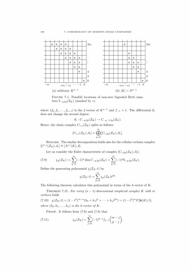
108 7. COHOMOLOGY OF MOMENT-ANGLE COMPLEXES
0
2
4
...
2m
0−1· · ·−(m− n)−m
∗
∗∗
∗∗
∗∗
∗
∗∗
∗∗
∗∗
∗∗
∗∗
∗
∗∗
∗∗
(a) arbitrary Kn−1
0
2
4
...
2m
0−1· · ·−(m− n)−m
∗
∗∗
∗∗
∗∗
∗∗
∗
∗
(b) |K| = Sn−1
Figure 7.1. Possible locations of non-zero bigraded Betti num-bers b−q,2p(ZK) (marked by ∗).
where (f0, f1, . . . , fn−1) is the f -vector of Kn−1 and f−1 = 1. The differential ∂c
does not change the second degree:
∂c : C−q,2p(ZK) → C−q−1,2p(ZK).
Hence, the chain complex C∗,∗(ZK) splits as follows:
[C∗,∗(ZK), ∂c] =m⊕
p=0
[C∗,2p(ZK), ∂c
].
Remark. The similar decomposition holds also for the cellular cochain complex[C∗,∗(ZK), dc] ∼= [A∗,∗(K), d].
Let us consider the Euler characteristic of complex [C∗,2p(ZK), ∂c]:
(7.9) χp(ZK) :=m∑
q=0
(−1)q dim C−q,2p(ZK) =m∑
q=0
(−1)qb−q,2p(ZK).
Define the generating polynomial χ(ZK ; t) by
χ(ZK ; t) =m∑
p=0
χp(ZK)t2p.
The following theorem calculates this polynomial in terms of the h-vector of K.
Theorem 7.15. For every (n − 1)-dimensional simplicial complex K with mvertices holds
(7.10) χ(ZK ; t) = (1− t2)m−n(h0 + h1t2 + · · ·+ hnt2n) = (1− t2)mF
(k(K); t
),
where (h0, h1, . . . , hn) is the h-vector of K.
Proof. It follows from (7.9) and (7.8) that
(7.11) χp(ZK) =m∑
j=0
(−1)p−jfj−1
(m− j
p− j
),
7.3. BIGRADED BETTI NUMBERS OF ZK : THE CASE OF GENERAL K 109
Then
(7.12) χ(ZK ; t) =m∑
p=0
χp(K)t2p =m∑
p=0
m∑
j=0
t2jt2(p−j)(−1)p−jfj−1
(m− j
p− j
)
=m∑
j=0
fj−1t2j(1− t2)m−j = (1− t2)m
n∑
j=0
fj−1(t−2 − 1)−j .
Denote h(t) = h0 + h1t + · · ·+ hntn. From (1.7) we get
tnh(t−1) = (t− 1)nn∑
i=0
fi−1(t− 1)−i.
Substituting t−2 for t above, we finally rewrite (7.12) as
χ(ZK ; t)(1− t2)m
=t−2nh(t2)(t−2 − 1)n
=h(t2)
(1− t2)n,
which is equivalent to the first identity from (7.10). The second identity followsfrom Lemma 3.8. ¤
The formula from the above theorem can be used to express the face vector ofa simplicial complex in terms of the bigraded Betti numbers of the correspondingmoment-angle complex ZK .
Corollary 7.16. The Euler characteristic of ZK is zero.
Proof. We have
χ(ZK) =m∑
p,q=0
(−1)−q+2pb−q,2p(ZK) =m∑
p=0
χp(ZK) = χ(ZK ; 1),
so the statement follows from (7.10). ¤Remark. Another proof of the above corollary follows from the observation
that the diagonal subgroup S1 ⊂ Tm always acts freely on ZK (see section 7.5).Hence, there exists a principal S1-bundle ZK → ZK/S1, which implies χ(ZK) = 0.
The torus Z∅ = ρ−1(1, . . . , 1) ∼= Tm is a cellular subcomplex of ZK , seeLemma 6.18. The cellular cochain subcomplex C∗(Z∅) ⊂ C∗(ZK) ∼= A∗(K) hasthe basis consisting of cochains T (∅, τ)∗ and is mapped to the exterior algebraΛ[u1, . . . , um] ⊂ A∗(K) under the isomorphism of Theorem 7.11. It follows thatthere is an isomorphism of k-modules
(7.13) C∗(ZK ,Z∅) ∼= A∗(K)/Λ[u1, . . . , um].
We introduce relative bigraded Betti numbers
(7.14) b−q,2p(ZK ,Z∅) = dim H−q,2p[C∗(ZK ,Z∅), d
], q, p = 0, . . . , m,
define the p-th relative Euler characteristic χp(ZK ,Z∅) by
(7.15) χp(ZK ,Z∅) =m∑
q=0
(−1)q dim C−q,2p(ZK ,Z∅) =m∑
q=0
(−1)qb−q,2p(ZK ,Z∅),
and define the corresponding generating polynomial:
χ(ZK ,Z∅; t) =m∑
p=0
χp(ZK ,Z∅)t2p.
110 7. COHOMOLOGY OF MOMENT-ANGLE COMPLEXES
Theorem 7.17. For any (n − 1)-dimensional simplicial complex K with mvertices holds
(7.16) χ(ZK ,Z∅; t) = (1− t2)m−n(h0 + h1t2 + · · ·+ hnt2n)− (1− t2)m.
Proof. Since C∗(Z∅) = Λ[u1, . . . , um] and bideg ui = (−1, 2), we have
dim C−q(Z∅) = dim C−q,2q(Z∅) =(mq
).
Combining (7.13), (7.9) and (7.15), we get
χp(ZK ,Z∅) = χp(ZK)− (−1)p dim C−p,2p(Z∅).
Hence,
χ(ZK ,Z∅; t) = χ(ZK ; t)−m∑
p=0
(−1)p(mp
)t2p
= (1− t2)m−n(h0 + h1t2 + · · ·+ hnt2n)− (1− t2)m,
by (7.10). ¤
We will use the above theorem in section 7.6.
7.4. Bigraded Betti numbers of ZK : the case of spherical K
If K is a simplicial sphere then ZK is a manifold (Lemma 6.13). This im-poses additional conditions on the cohomology of ZK and leads to some interestinginterpretations of combinatorial results and problems from chapters 2 and 3.
Theorem 7.18. Let K be an (n − 1)-dimensional simplicial sphere, and ZK
the corresponding moment-angle manifold, dimZK = m+n. Then the fundamentalcohomology class of ZK is represented by any monomial ±vσuτ ∈ A∗(K) of bidegree(−(m − n), 2m) such that σ is an (n − 1)-simplex of K and σ ∩ τ = ∅. The signdepends on a choice of orientation for ZK .
Proof. Lemma 7.14 (f) shows that Hm+n(ZK) = H−(m−n),2m(ZK). Themodule A−(m−n),2m(K) is spanned by the monomials vσuτ such that σ ∈ Kn−1,|σ| = n, τ = [m] \ σ. Every such monomial is a cocycle. Suppose that σ, σ′ aretwo (n − 1)-simplices of Kn−1 sharing a common (n − 2)-face. We claim that thecorresponding cocycles vσuτ , vσ′uτ ′ (where τ = [m] \ σ, τ ′ = [m] \ σ′) representthe same cohomology class up to a sign. Indeed, let
vσuτ = vi1 · · · vinuj1 · · ·ujm−n ,
vσ′uτ ′ = vi1 · · · vin−1vj1uinuj2 · · ·ujm−n .
Since every (n− 2)-face of K is contained in exactly two (n− 1)-faces, the identity
d(vi1 · · · vin−1uinuj1uj2 · · ·ujm−n)= vi1 · · · vinuj1 · · ·ujm−n − vi1 · · · vin−1vj1uinuj2 · · ·ujm−n
holds in A∗(K) ⊂ Λ[u1, . . . , um] ⊗ k(K). Hence, [vσuτ ] = [vσ′uτ ′ ] (as cohomologyclasses). Since Kn−1 is a simplicial sphere, every two (n − 1)-simplices can beconnected by a chain of simplices in such a way that any two successive simplicesshare a common (n−2)-face. Thus, all monomials vσuτ in A−(m−n),2m(K) representthe same cohomology class (up to a sign). This class is a generator of Hm+n(ZK),i.e. the fundamental cohomology class of ZK . ¤
7.4. BIGRADED BETTI NUMBERS OF ZK : THE CASE OF SPHERICAL K 111
Remark. In the above proof we have used two combinatorial properties ofKn−1. The first one is that every (n− 2)-face is contained in exactly two (n− 1)-faces, and the second is that every two (n − 1)-simplices can be connected by achain of simplices with any two successive simplices sharing a common (n−2)-face.Simplicial complexes satisfying these two conditions are called pseudomanifolds.In particular, every triangulated manifold is a pseudomanifold. Hence, for anytriangulated manifold Kn−1 we have bm+n(ZK) = b−(m−n),2m(ZK) = 1, and thegenerator of Hm+n(ZK) can be chosen as described in Theorem 7.18.
Corollary 7.19. The Poincare duality for the moment angle manifold ZK
corresponding to a simplicial sphere Kn−1 respects the bigraded structure in the(co)homology, i.e.
H−q,2p(ZK) ∼= H−(m−n)+q,2(m−p)(ZK).
In particular,
(7.17) b−q,2p(ZK) = b−(m−n)+q,2(m−p)(ZK). ¤
Corollary 7.20. Let Kn−1 be an (n− 1)-dimensional simplicial sphere, andZK the corresponding moment-angle complex, dimZK = m + n. Then
(a) b−q,2p(ZK) = 0 for q ≥ m− n, with only exception b−(m−n),2m = 1;(b) b−q,2p(ZK) = 0 for p− q ≥ n, with only exception b−(m−n),2m = 1.
It follows that if Kn−1 is a simplicial sphere, then non-zero bigraded Bettinumbers br,2p(ZK) with r 6= 0 and r 6= m− n appear only in the strip bounded bythe lines r = −(m − n − 1), r = −1, p + r = 1 and p + r = n − 1 in the secondquadrant, see Figure 7.1 (b). Compare this with Figure 7.1 (a) corresponding tothe case of general K.
Example 7.21. Let K = ∂∆m−1. Then k(K) = k[v1, . . . , vm]/(v1 · · · vm),see Example 3.9. A direct calculation shows that the cohomology H[k(K) ⊗Λ[u1, . . . , um], d] (see Theorem 7.7) is additively generated by the classes 1 and[v1v2 · · · vm−1um]. We have deg(v1v2 · · · vm−1um) = 2m−1, and Theorem 7.18 saysthat v1v2 · · · vm−1um represents the fundamental cohomology class of ZK
∼= S2m−1.
Example 7.22. Let K be the boundary complex of an m-gon P 2 with m ≥ 4.We have k(K) = k[v1, . . . , vm]/IP , where IP is generated by the monomials vivj ,i− j 6= 0, 1 mod m. The complex ZK = ZP is a manifold of dimension m+2. TheBetti numbers of these manifolds were calculated in [31]. Namely,
(7.18) dim Hk(ZP ) =
1 for k = 0,m + 2;0 for k = 1, 2,m, m + 1;
(m− 2)(m−2k−2
)− (m−2k−1
)− (m−2k−3
)for 3 ≤ k ≤ m− 1.
For example, in the case m = 5 the group H3(ZP ) has 5 generators representedby the cocycles viui+2 ∈ k(K) ⊗ Λ[u1, . . . , u5], i = 1, . . . , 5, while the groupH4(ZP ) has 5 generators represented by the cocycles vjuj+2uj+3, j = 1, . . . , 5.As it follows from Theorem 7.18, the product of cocycles viui+2 and vjuj+2uj+3
represents a non-zero cohomology class in H7(ZP ) if and only if all the indicesi, i + 2, j, j + 2, j + 3 are different. Thus, for each of the 5 cohomology classes[viui+2] there is a unique (Poincare dual) cohomology class [vjuj+2uj+3] such thatthe product [viui+2] · [vjuj+2uj+3] is non-zero. This observation has the following
112 7. COHOMOLOGY OF MOMENT-ANGLE COMPLEXES
generalization, which describes the multiplicative structure in the cohomology ofZP 2 for any m-gon P 2.
Proposition 7.23 (Cohomology ring of ZP 2). Let P 2 be an m-gon, m ≥ 4.(a) The only non-zero bigraded cohomology groups of ZP 2 are H0,0(= H0),
H−p,2(p+1)(= Hp+2) for p = 1, . . . , m− 3, and H−m+2,2m(= Hm+2).(b) The group H−p,2(p+1) is free and is generated by the cohomology classes
[viuτ ] such that |τ | = p, i /∈ τ and i±1 /∈ τ . These cohomology classes aresubject to relations of the form duτ ′ = 0 for |τ ′| = p+1. The correspondingBetti numbers are given by (7.18).
(c) The group H−m+2,2m is one-dimensional with generator [v1v2u3 · · ·um].(d) The product of two cohomology classes [vi1uτ1 ] ∈ H−p1,2(p1+1) and [vi2uτ2 ] ∈
H−p2,2(p2+1) equals [v1v2u3 · · ·um] (up to a sign) if i1, i2, τ1, τ2 isa partition of [m], and zero otherwise.
Therefore, the only non-trivial products in the ring H∗(ZP 2) are those which givea multiple of the fundamental class.
Proof. Statement (a) follows from Corollary 7.20, (b) is obvious, and (c)follows from Theorem 7.18. In order to prove (d) we mention that the product of twoclasses a1 ∈ H−p1,2(p1+1) and a2 ∈ H−p2,2(p2+1) has bidegree (−p, 2q) with q−p = 2,whence it can be non-zero only if it belongs to H−m+2,2m, by Corollary 7.20. ¤
It follows from (7.9) and (7.17) that for any simplicial sphere K holds
χp(ZK) = (−1)m−nχm−p(ZK).
¿From this and (7.10) we get
h0 + h1t2 + · · ·+ hnt2n
(1− t2)n= (−1)m−n χm + χm−1t
2 + · · ·+ χ0t2m
(1− t2)m
= (−1)n χ0 + χ1t−2 + · · ·+ χmt−2m
(1− t−2)m= (−1)n h0 + h1t
−2 + · · ·+ hnt−2n
(1− t−2)n
=h0t
2n + h1t2(n−1) + · · ·+ hn
(1− t2)n.
Hence, hi = hn−i. Thus, the Dehn–Sommerville equations are a corollary of thebigraded Poincare duality (7.17).
The identity (7.10) also allows to interpret different inequalities for the f -vectors of simplicial spheres or triangulated manifolds in terms of topological in-variants (the bigraded Betti numbers) of the corresponding moment-angle manifolds(or complexes) ZK .
Example 7.24. Using the expansion(
11− t2
)m−n
=∞∑
i=0
(m− n + i− 1
i
)t2i
together with the UBC for simplicial spheres (Corollary 3.19) and identity (7.10),we deduce that the inequality χ(ZK ; t) ≤ 1 holds coefficient-wise for any simplicialsphere Kn−1. That is,
χi(ZK ; t) ≤ 0 for i > 0.
7.5. PARTIAL QUOTIENTS OF ZP 113
Example 7.25. Using Lemma 7.14 we calculate
χ0(ZK) = 1, χ1(ZK) = 0,
χ2(ZK) = −b−1,4(ZK) = −b3(ZK), χ3(ZK) = b−2,6(ZK)− b−1,6(ZK)
(note that b4(ZK) = b−2,6(ZK) and b5(ZK) = b−1,6(ZK) + b−3,8(ZK)). Now,identity (7.10) shows that
h0 = 1,
h1 = m− n,
h2 =(m−n+1
2
)− b3(ZK),
h3 =(m−n+2
3
)− (m− n)b−1,4(ZK) + b−2,6(ZK)− b−1,6(ZK).
It follows that the inequality h1 ≤ h2 (n ≥ 4) from the GLBC (1.14) for simplicialspheres is equivalent to the following:
(7.19) b3(ZK) ≤ (m−n
2
).
(Note that this inequality is not valid for n = 2, see e.g. Example 7.22, and becomesidentity for n = 3.) The next inequality h2 ≤ h3 (n ≥ 6) from (1.14) is equivalentto the following:
(7.20)(m−n+1
3
)− (m− n− 1)b−1,4(ZK) + b−2,6(ZK)− b−1,6(ZK) ≥ 0.
We see that the combinatorial GLBC inequalities are interpreted as “topologi-cal” inequalities for the (bigraded) Betti numbers of a manifold. This might opena possibility to use topological methods (such as the equivariant topology or Morsetheory) for proving inequalities like (7.19) or (7.20). Such a topological approachto problems like g-conjecture or GLBC has an advantage of being independenton whether the simplicial sphere K is polytopal or not. Indeed, as we have al-ready mentioned, all known proofs for the necessity condition in the g-theorem forsimplicial polytopes (including the original one by Stanley given in section 5.1, Mc-Mullen’s proof [97], and the recent proof by Timorin [133]) follow the same scheme.Namely, the numbers hi, i = 1, . . . , n, are interpreted as the dimensions of gradedcomponents Ai of a certain algebra A satisfying the Hard Lefschetz Theorem. Thelatter means that there is an element ω ∈ A1 such that the multiplication by ω de-fines a monomorphism Ai → Ai+1 for i <
[n2
]. This implies hi ≤ hi+1 for i <
[n2
](see section 5.1). However, such an element ω is lacking for non-polytopal K, whichmeans that a new technique has to be developed in order to prove the g-conjecturefor simplicial spheres.
As it was mentioned in section 3.5, simplicial spheres are Gorenstein* com-plexes. Using theorems 3.38, 3.39 and our Theorem 7.6 we obtain the followinganswer to a weaker version of Problem 6.14.
Proposition 7.26. The complex ZK is a Poincare duality complex (over k) ifand only if K is Gorenstein*, i.e., for any simplex σ ∈ K (including σ = ∅) thesubcomplex linkσ has the homology of a sphere of dimension dim (link σ).
7.5. Partial quotients of ZP
Here we return to the case of polytopal K (i.e. K = KP for some simplepolytope P ) and study quotients of ZP by freely acting subgroups H ⊂ Tm.
114 7. COHOMOLOGY OF MOMENT-ANGLE COMPLEXES
For any combinatorial simple polytope Pn, define s = s(Pn) to be the maximaldimension for which there exists a subgroup H ∼= T s in Tm acting freely on ZP .The number s(Pn) is obviously a combinatorial invariant of Pn.
Problem 7.27 (V. M. Buchstaber). Provide an efficient way to calculate thenumber s(Pn), e.g. in terms of known combinatorial invariants of Pn.
Proposition 7.28. If Pn has m facets, then s(Pn) ≤ m− n.
Proof. Every subtorus of Tm of dimension > m − n intersects non-triviallywith any n-dimensional isotropy subgroup, and therefore can not act freely on ZP .
¤
Proposition 7.29. The diagonal circle subgroup Sd := (e2πiϕ, . . . , e2πiϕ) ∈Tm, ϕ ∈ R, acts freely on any ZP . Thus, s(Pn) ≥ 1.
Proof. By Definition 6.1, every isotropy subgroup for ZP is coordinate, andtherefore intersects Sd only at the unit. ¤
An alternative lower bound for the number s(Pn) was proposed in [79]. LetF = F1, . . . , Fm be the set of facets of Pn. We generalize the definition of aregular coloring from section 6.6 as follows. A surjective map % : F → [k] (where[k] = 1, . . . , k) is called a regular k-paint coloring of Pn if %(Fi) 6= %(Fj) wheneverFi∩Fj 6= ∅. The chromatic number γ(Pn) is the minimal k for which there exists aregular k-paint coloring of Pn. Then γ(Pn) ≥ n and, due to the result mentioned insection 6.6, the equality is achieved if and only if every 2-face of Pn is an evengon.Note also that γ(P 3) ≤ 4 by the Four Color Theorem.
Example 7.30. Suppose Pn is a 2-neighborly simple polytope with m facets.Then γ(Pn) = m.
Proposition 7.31 ([79]). The following inequality holds:
s(Pn) ≥ m− γ(Pn).
Proof. The map % : F → [k] defines an epimorphism of tori % : Tm → T k.It is easy to see that if % is a regular coloring, then Ker % ∼= Tm−k acts freelyon ZP . ¤
For more results on colorings and their relations with Problem 7.27 see [81].Let H ⊂ Tm be a subgroup of dimension r ≤ m− n. Choosing a basis, we can
write it in the form
(7.21) H =(e2πi(s11ϕ1+···+s1rϕr), . . . , e2πi(sm1ϕ1+···+smrϕr)) ∈ Tm
,
where ϕi ∈ R, i = 1, . . . , r. The integer m × r-matrix S = (sij) defines amonomorphism Zr → Zm whose image is a direct summand in Zm. For any subseti1, . . . , in ⊂ [m] denote by Si1,...,in
the (m − n) × r submatrix of S obtained bydeleting the rows i1, . . . , in. Write each vertex v ∈ Pn as an intersection of n facets,as in (5.10). The following criterion of freeness for the action of H on ZP holds.
Lemma 7.32. Subgroup (7.21) acts freely on ZP if and only if for every vertexv = Fi1∩. . .∩Fin of Pn the (m−n)×r-submatrix Si1,...,in
defines a monomorphismZr → Zm−n to a direct summand.
7.5. PARTIAL QUOTIENTS OF ZP 115
Proof. It follows from Definition 6.1 that the orbits of Tm-action on ZP
corresponding to the vertices of Pn have maximal (rank n) isotropy subgroups. Theisotropy subgroup corresponding to a vertex v = Fi1 ∩ . . . ∩ Fin
is the coordinatesubtorus Tn
i1,...,in⊂ Tm. Subgroup (7.21) acts freely on ZP if and only if it intersects
each isotropy subgroup only at the unit. This is equivalent to the condition that themap H×Tn
i1,...,in→ Tm is injective for any v = Fi1∩ . . .∩Fin . This map is given by
the integer m× (n + r)-matrix obtained by adding n columns (0, . . . , 0, 1, 0, . . . , 0)t
(with 1 at the place ij , j = 1, . . . , n) to S. The map is injective if and only if thisenlarged matrix defines a direct summand in Zm. The latter holds if and only ifeach Si1,...,in
defines a direct summand. ¤
In particular, for subgroups of rank m− n we get the following statement.
Corollary 7.33. The subgroup (7.21) of rank r = m− n acts freely on ZP ifand only if for any vertex v = Fi1 ∩ . . . ∩ Fin
of Pn holds detSi1...in= ±1.
Proposition 7.34. A simple polytope Pn admits a characteristic map if andonly if s(Pn) = m− n.
Proof. Proposition 6.5 shows that if Pn admits a characteristic map `, thenthe (m−n)-dimensional subgroup H(`) acts freely on ZP , whence s(Pn) = m−n.Now suppose s(Pn) = m − n, i.e. there exists a subgroup (7.21) of rank r =m − n that acts freely on ZP . The corresponding m × (m − n)-matrix S definesa monomorphism Zm−n → Zm whose image is a direct summand. It follows thatthere is an n×m-matrix Λ such that the sequence
0 −−−−→ Zm−n S−−−−→ Zm Λ−−−−→ Zn −−−−→ 0is exact. Since S satisfies the condition of Corollary 7.33, the matrix Λ satisfies (5.5),thus defining a characteristic map for Pn. ¤
Suppose M2n is a quasitoric manifold over Pn with characteristic map `. Writethe subgroup H(`) in the form (7.21). Now define the following linear forms ink[v1, . . . , vm]:
(7.22) wi = s1iv1 + · · ·+ smivm, i = 1, . . . , m− n.
Under these assumptions the following statement holds.
Lemma 7.35. There is the following isomorphism of algebras:
H∗(ZP ) ∼= Tork[w1,...,wm−n]
(H∗(M2n),k
),
where the k[w1, . . . , wm−n]-module structure in H∗(M2n) = k[v1, . . . , vm]/IP +J`
is defined by (7.22).
Proof. By Theorem 7.13,
H∗(ZK) ∼= Tork[v1,...,vm]/J`
(k(K)/J`,k
).
The quotient k[v1, . . . , vm]/J` is identified with k[w1, . . . , wm−n]. ¤
Theorem 7.36. The Leray–Serre spectral sequence of the Tm−n-bundle ZP →M2n collapses at the E3 term. Furthermore, the following isomorphism of algebrasholds:
H∗(ZP ) ∼= H[Λ[u1, . . . , um−n]⊗ (
k(P )/J`
), d
],
116 7. COHOMOLOGY OF MOMENT-ANGLE COMPLEXES
where
bideg vi = (0, 2), bideg ui = (−1, 2);
d(ui) = wi, d(vi) = 0.
Proof. Since H∗(Tm−n) = Λ[u1, . . . , um−n] and H∗(M2n) = k(P )/J`, wehave
E3∼= H
[(k(P )/J`)⊗ Λ[u1, . . . , um−n], d
].
By Lemma 3.29,
H[(k(P )/J`)⊗ Λ[u1, . . . , um−n], d
] ∼= Tork[w1,...,wm−n]
(H∗(M2n),k
).
Combining the above two identities with Lemma 7.35 we get E3 = H∗(ZP ), whichconcludes the proof. ¤
Our next aim is to calculate the cohomology of the quotient ZP /H for arbitraryfreely acting subgroup H. First, we write H in the form (7.21) and choose an(m− r)×m-matrix T = (tij) of rank (m− r) satisfying T · S = 0. This is done inthe same way as in the proof of Proposition 7.34. In particular, if r = m− n thenT is the characteristic matrix for the quasitoric manifold ZP /H.
Theorem 7.37. The following isomorphism of algebras holds:
H∗(ZP /H) ∼= Tork[t1,...,tm−r ]
(k(P ),k
),
where the k[t1, . . . , tm−r]-module structure on k(P ) = k[v1, . . . , vm]/IP is given bythe map
k[t1, . . . , tm−r] → k[v1, . . . , vm]ti → ti1v1 + · · ·+ timvm.
Remark. Theorem 7.37 reduces to Theorem 7.6 in the case r = 0 and toExample 7.5 in the case r = m− n.
Proof of Theorem 7.37. The inclusion T r ∼= H → Tm defines the maph : BT r → BTm of the classifying spaces. Let us consider the commutative square
E −−−−→ BT Py
yp
BT r h−−−−→ BTm,
where the left vertical arrow is the pullback along h. The space E is homotopyequivalent to the quotient ZP /H. Hence, the Eilenberg–Moore spectral sequenceof the above square converges to the cohomology of ZP /H. Its E2-term is
E2 = Tork[v1,...,vm]
(k(P ),k[w1, . . . , wr]
),
where the k[v1, . . . , vm]-module structure in k[w1, . . . , wr] is defined by the ma-trix S, i.e. by the map vi → si1w1 + . . .+ sirwr. In the same way as in the proof ofTheorem 7.6 we show that the spectral sequence collapses at the E2 term and thefollowing isomorphism of algebras holds:
(7.23) H∗(ZP /H) = Tork[v1,...,vm]
(k(P ),k[w1, . . . , wr]
).
7.6. BIGRADED POINCARE DUALITY AND DEHN–SOMMERVILLE EQUATIONS 117
Now put Λ = k[v1, . . . , vm], Γ = k[t1, . . . , tm−r], A = k[w1, . . . , wr] and C = k(P )in Theorem 3.36. Since Λ is a free Γ-module and Ω = Λ//Γ ∼= k[w1, . . . , wr], aspectral sequence Es, ds arises. Its E2 term is
E2 = Tork[w1,...,wr]
(k[w1, . . . , wr],Tork[t1,...,tm−r ]
(k(P ),k
)),
and it converges to Tork[v1,...,vm](k(P ),k[w1, . . . , wr]). Obviously, k[w1, . . . , wr] isa free k[w1, . . . , wr]-module, so we have
Ep,q2 = 0 for p 6= 0, E0,∗
2 = Tork[t1,...,tm−r]
(k(P ),k
).
Thus, the spectral sequence collapses at the E2 term, and the following isomorphismof algebras holds:
Tork[v1,...,vm]
(k(P ),k[w1, . . . , wr]
) ∼= Tork[t1,...,tm−r]
(k(P ),k
),
which together with (7.23) concludes the proof. ¤Corollary 7.38. H∗(ZP /H) ∼= H
[Λ[u1, . . . , um−r]⊗ k(Pn), d
], where dui =
(ti1v1 + . . . + timvm), dvi = 0, bideg vi = (0, 2), bideg ui = (−1, 2).
Example 7.39. Let H = Sd is the diagonal subgroup. Then the matrix S is acolumn of m units. By Theorem 7.37,
(7.24) H∗(ZP /Sd) ∼= Tork[t1,...,tm−1]
(k(P ),k
),
where the k[t1, . . . , tm−1]-module structure in k(P ) = k[v1, . . . , vm]/I is defined by
ti −→ vi − vm, i = 1, . . . ,m− 1.
Suppose that the S1-bundle ZP → ZP /Sd is classified by a map c : ZP /Sd →BT 1 ∼= CP∞. Since H∗(CP∞) ∼= k[w], the element c∗(w) ∈ H2(ZP /Sd) is defined.
Lemma 7.40. Pn is q-neighborly if and only if (c∗(w))q 6= 0.
Proof. The map c∗ takes the cohomology ring H∗(BT 1) ∼= k[w] to the sub-algebra
k(P )⊗k[t1,...,tm−1] k = Tor0k[t1,...,tm−1]
(k(P ),k
) ⊂ H∗(ZP /H)
This subalgebra is isomorphic to the quotient k(P )/(v1 = · · · = vm). Now theassertion follows from the fact that a polytope Pn is q-neighborly if and only if theideal IP does not contain monomials of degree < q + 1. ¤
7.6. Bigraded Poincare duality and Dehn–Sommerville equations
Here we assume that Kn−1 is a triangulated manifold. In this case the cor-responding moment-angle complex ZK is not a manifold in general, however, itssingularities can be easily treated. Indeed, the cubical complex cc(K) (Construc-tion 4.9) is homeomorphic to | cone(K)| and the vertex of the cone is p = (1, . . . , 1) ∈cc(K) ⊂ Im. Let Uε(p) ⊂ cc(K) be a small neighborhood of p in cc(K). The clo-sure of Uε(p) is also homeomorphic to | cone(K)|. It follows from the definition ofZK (see (6.3)) that Uε(Z∅) := ρ−1(Uε(p)) ⊂ ZK is a small invariant neighborhoodof the torus Z∅ = ρ−1(p) ∼= Tm in ZK . For small ε the closure of Uε(Z∅) is home-omorphic to | cone(K)| × Tm. Removing Uε(Z∅) from ZK we obtain a manifoldwith boundary, which we denote WK . Thus, we have
WK = ZK \ Uε(Z∅), ∂WK∼= |K| × Tm.
Note that since Uε(Z∅) is a Tm-stable subset, the torus Tm acts on WK .
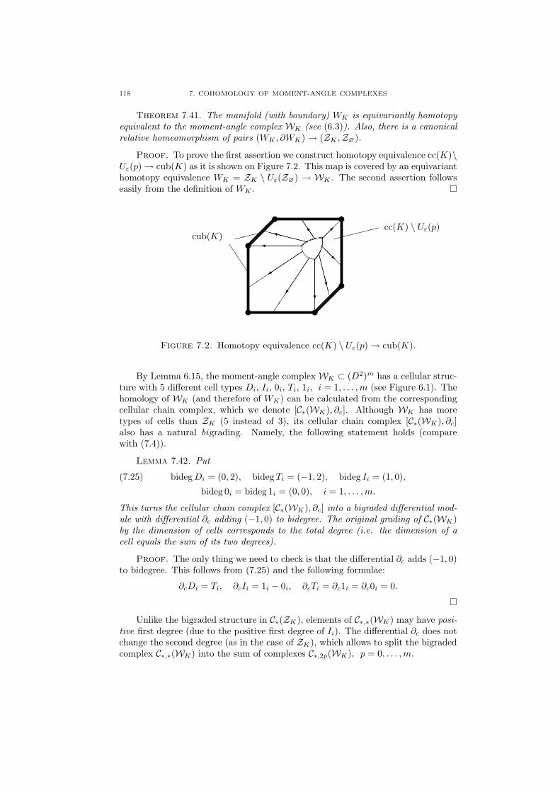
118 7. COHOMOLOGY OF MOMENT-ANGLE COMPLEXES
Theorem 7.41. The manifold (with boundary) WK is equivariantly homotopyequivalent to the moment-angle complex WK (see (6.3)). Also, there is a canonicalrelative homeomorphism of pairs (WK , ∂WK) → (ZK ,Z∅).
Proof. To prove the first assertion we construct homotopy equivalence cc(K)\Uε(p) → cub(K) as it is shown on Figure 7.2. This map is covered by an equivarianthomotopy equivalence WK = ZK \ Uε(Z∅) → WK . The second assertion followseasily from the definition of WK . ¤
u
u
u
u
u
u
¡¡
¡
¡¡
¡
¡¡
¡
¡¡
¡
¡¡
¡
¡¡
¡
¡¡
¡
¡¡
¡
¡¡
¡
¡¡
¡
¡¡
¡
¡¡
¡
¡¡
¡
¡¡
¡
¡¡
¡
¡¡
¡
¡¡
¡
¡¡
¡
¡¡
¡
¡¡
¡
¡¡
¡
¡¡
¡
¡¡
¡
¡¡
¡
¡¡
¡
¡¡
¡
¡¡
¡
¡¡
¡
¡¡
¡
¡¡
¡
¡¡
¡
¡¡
¡
¡¡µ¡¡
¾
?
´´
´´
´
´´
´+
À
XXXXXJ
JJXXXXy JJ]
CCCCC
@@C
CCCW
@@R½
»»»»» cc(K) \ Uε(p)
JJ
J
»»»cub(K)
Figure 7.2. Homotopy equivalence cc(K) \ Uε(p) → cub(K).
By Lemma 6.15, the moment-angle complex WK ⊂ (D2)m has a cellular struc-ture with 5 different cell types Di, Ii, 0i, Ti, 1i, i = 1, . . . , m (see Figure 6.1). Thehomology of WK (and therefore of WK) can be calculated from the correspondingcellular chain complex, which we denote [C∗(WK), ∂c]. Although WK has moretypes of cells than ZK (5 instead of 3), its cellular chain complex [C∗(WK), ∂c]also has a natural bigrading. Namely, the following statement holds (comparewith (7.4)).
Lemma 7.42. Put
bideg Di = (0, 2), bideg Ti = (−1, 2), bideg Ii = (1, 0),(7.25)
bideg 0i = bideg 1i = (0, 0), i = 1, . . . , m.
This turns the cellular chain complex [C∗(WK), ∂c] into a bigraded differential mod-ule with differential ∂c adding (−1, 0) to bidegree. The original grading of C∗(WK)by the dimension of cells corresponds to the total degree (i.e. the dimension of acell equals the sum of its two degrees).
Proof. The only thing we need to check is that the differential ∂c adds (−1, 0)to bidegree. This follows from (7.25) and the following formulae:
∂cDi = Ti, ∂cIi = 1i − 0i, ∂cTi = ∂c1i = ∂c0i = 0.
¤
Unlike the bigraded structure in C∗(ZK), elements of C∗,∗(WK) may have posi-tive first degree (due to the positive first degree of Ii). The differential ∂c does notchange the second degree (as in the case of ZK), which allows to split the bigradedcomplex C∗,∗(WK) into the sum of complexes C∗,2p(WK), p = 0, . . . ,m.
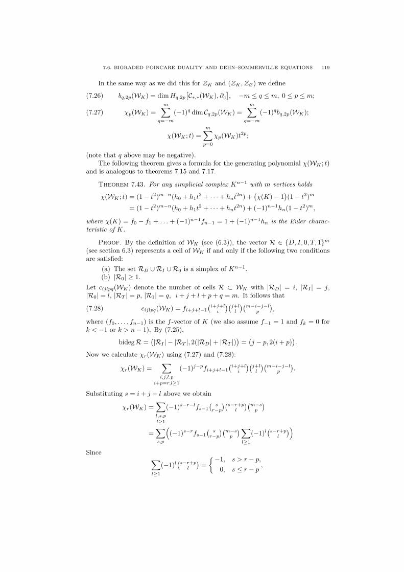
7.6. BIGRADED POINCARE DUALITY AND DEHN–SOMMERVILLE EQUATIONS 119
In the same way as we did this for ZK and (ZK ,Z∅) we define
bq,2p(WK) = dim Hq,2p
[C∗,∗(WK), ∂c
], −m ≤ q ≤ m, 0 ≤ p ≤ m;(7.26)
χp(WK) =m∑
q=−m
(−1)q dim Cq,2p(WK) =m∑
q=−m
(−1)qbq,2p(WK);(7.27)
χ(WK ; t) =m∑
p=0
χp(WK)t2p;
(note that q above may be negative).The following theorem gives a formula for the generating polynomial χ(WK ; t)
and is analogous to theorems 7.15 and 7.17.
Theorem 7.43. For any simplicial complex Kn−1 with m vertices holds
χ(WK ; t) = (1− t2)m−n(h0 + h1t2 + · · ·+ hnt2n) +
(χ(K)− 1
)(1− t2)m
= (1− t2)m−n(h0 + h1t2 + · · ·+ hnt2n) + (−1)n−1hn(1− t2)m,
where χ(K) = f0 − f1 + . . . + (−1)n−1fn−1 = 1 + (−1)n−1hn is the Euler charac-teristic of K.
Proof. By the definition of WK (see (6.3)), the vector R ∈ D, I, 0, T, 1m
(see section 6.3) represents a cell of WK if and only if the following two conditionsare satisfied:
(a) The set RD ∪RI ∪R0 is a simplex of Kn−1.(b) |R0| ≥ 1.
Let cijlpq(WK) denote the number of cells R ⊂ WK with |RD| = i, |RI | = j,|R0| = l, |RT | = p, |R1| = q, i + j + l + p + q = m. It follows that
(7.28) cijlpq(WK) = fi+j+l−1
(i+j+l
i
)(j+l
l
)(m−i−j−l
p
),
where (f0, . . . , fn−1) is the f -vector of K (we also assume f−1 = 1 and fk = 0 fork < −1 or k > n− 1). By (7.25),
bidegR =(|RI | − |RT |, 2(|RD|+ |RT |)
)=
(j − p, 2(i + p)
).
Now we calculate χr(WK) using (7.27) and (7.28):
χr(WK) =∑
i,j,l,p
i+p=r,l≥1
(−1)j−pfi+j+l−1
(i+j+l
i
)(j+l
l
)(m−i−j−l
p
).
Substituting s = i + j + l above we obtain
χr(WK) =∑
l,s,p
l≥1
(−1)s−r−lfs−1
(s
r−p
)(s−r+p
l
)(m−s
p
)
=∑s,p
((−1)s−rfs−1
(s
r−p
)(m−s
p
) ∑
l≥1
(−1)l(s−r+p
l
))
Since∑
l≥1
(−1)l(s−r+p
l
)=
−1, s > r − p,
0, s ≤ r − p,
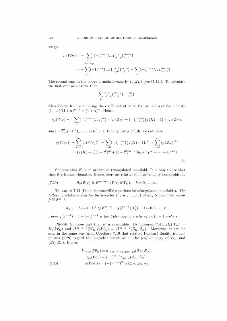
120 7. COHOMOLOGY OF MOMENT-ANGLE COMPLEXES
we get
χr(WK) = −∑s,p
s>r−p
(−1)s−rfs−1
(s
r−p
)(m−s
p
)
= −∑s,p
(−1)r−sfs−1
(s
r−p
)(m−s
p
)+
∑s
(−1)r−sfs−1
(m−sr−s
).
The second sum in the above formula is exactly χr(ZK) (see (7.11)). To calculatethe first sum we observe that
∑p
(s
r−p
)(m−s
p
)=
(mr
).
This follows from calculating the coefficient of αr in the two sides of the identity(1 + α)s(1 + α)m−s = (1 + α)m. Hence,
χr(WK) = −∑
s
(−1)r−sfs−1
(mr
)+ χr(ZK) = (−1)r
(mr
)(χ(K)− 1
)+ χr(ZK),
since −∑s(−1)sfs−1 = χ(K)− 1. Finally, using (7.10), we calculate
χ(WK ; t) =m∑
r=0
χr(WK)t2r =m∑
r=0
(−1)r(mr
)(χ(K)− 1
)t2r +
m∑r=0
χr(ZK)t2r
=(χ(K)− 1
)(1− t2)m + (1− t2)m−n(h0 + h1t
2 + · · ·+ hnt2n).
¤
Suppose that K is an orientable triangulated manifold. It is easy to see thatthen WK is also orientable. Hence, there are relative Poincare duality isomorphisms:
(7.29) Hk(WK) ∼= Hm+n−k(WK , ∂WK), k = 0, . . . , m.
Theorem 7.44 (Dehn–Sommerville equations for triangulated manifolds). Thefollowing relations hold for the h-vector (h0, h1, . . . , hn) of any triangulated mani-fold Kn−1:
hn−i − hi = (−1)i(χ(Kn−1)− χ(Sn−1)
)(ni
), i = 0, 1, . . . , n,
where χ(Sn−1) = 1 + (−1)n−1 is the Euler characteristic of an (n− 1)-sphere.
Proof. Suppose first that K is orientable. By Theorem 7.41, Hk(WK) =Hk(WK) and Hm+n−k(WK , ∂cWK) = Hm+n−k(ZK ,Z∅). Moreover, it can beseen in the same way as in Corollary 7.19 that relative Poincare duality isomor-phisms (7.29) regard the bigraded structures in the (co)homology of WK and(ZK ,Z∅). Hence,
b−q,2p(WK) = b−(m−n)+q,2(m−p)(ZK ,Z∅),
χp(WK) = (−1)m−nχm−p(ZK ,Z∅),
χ(WK ; t) = (−1)m−nt2mχ(ZK ,Z∅; 1t ).(7.30)
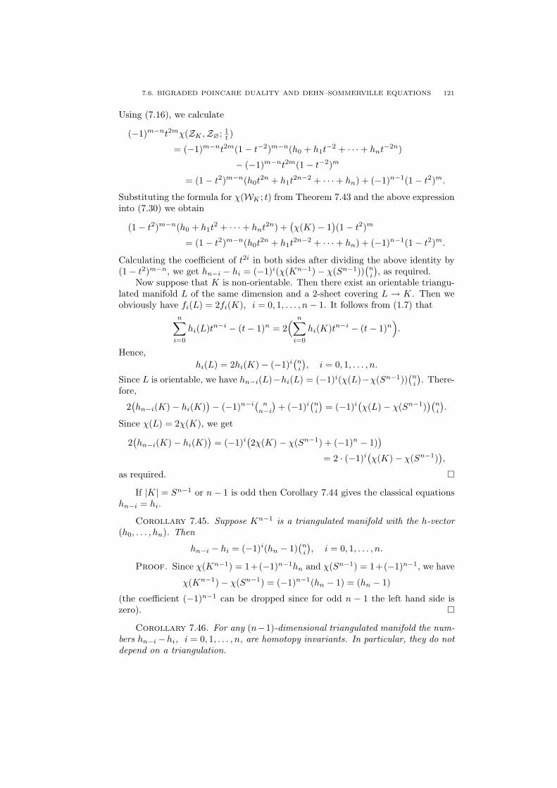
7.6. BIGRADED POINCARE DUALITY AND DEHN–SOMMERVILLE EQUATIONS 121
Using (7.16), we calculate
(−1)m−nt2mχ(ZK ,Z∅; 1t )
= (−1)m−nt2m(1− t−2)m−n(h0 + h1t−2 + · · ·+ hnt−2n)
− (−1)m−nt2m(1− t−2)m
= (1− t2)m−n(h0t2n + h1t
2n−2 + · · ·+ hn) + (−1)n−1(1− t2)m.
Substituting the formula for χ(WK ; t) from Theorem 7.43 and the above expressioninto (7.30) we obtain
(1− t2)m−n(h0 + h1t2 + · · ·+ hnt2n) +
(χ(K)− 1
)(1− t2)m
= (1− t2)m−n(h0t2n + h1t
2n−2 + · · ·+ hn) + (−1)n−1(1− t2)m.
Calculating the coefficient of t2i in both sides after dividing the above identity by(1− t2)m−n, we get hn−i − hi = (−1)i(χ(Kn−1)− χ(Sn−1))
(ni
), as required.
Now suppose that K is non-orientable. Then there exist an orientable triangu-lated manifold L of the same dimension and a 2-sheet covering L → K. Then weobviously have fi(L) = 2fi(K), i = 0, 1, . . . , n− 1. It follows from (1.7) that
n∑
i=0
hi(L)tn−i − (t− 1)n = 2( n∑
i=0
hi(K)tn−i − (t− 1)n).
Hence,hi(L) = 2hi(K)− (−1)i
(ni
), i = 0, 1, . . . , n.
Since L is orientable, we have hn−i(L)−hi(L) = (−1)i(χ(L)−χ(Sn−1))(ni
). There-
fore,
2(hn−i(K)− hi(K)
)− (−1)n−i(
nn−i
)+ (−1)i
(ni
)= (−1)i
(χ(L)− χ(Sn−1)
)(ni
).
Since χ(L) = 2χ(K), we get
2(hn−i(K)− hi(K)
)= (−1)i
(2χ(K)− χ(Sn−1) + (−1)n − 1)
)
= 2 · (−1)i(χ(K)− χ(Sn−1)
),
as required. ¤
If |K| = Sn−1 or n− 1 is odd then Corollary 7.44 gives the classical equationshn−i = hi.
Corollary 7.45. Suppose Kn−1 is a triangulated manifold with the h-vector(h0, . . . , hn). Then
hn−i − hi = (−1)i(hn − 1)(ni
), i = 0, 1, . . . , n.
Proof. Since χ(Kn−1) = 1+(−1)n−1hn and χ(Sn−1) = 1+(−1)n−1, we have
χ(Kn−1)− χ(Sn−1) = (−1)n−1(hn − 1) = (hn − 1)
(the coefficient (−1)n−1 can be dropped since for odd n − 1 the left hand side iszero). ¤
Corollary 7.46. For any (n−1)-dimensional triangulated manifold the num-bers hn−i−hi, i = 0, 1, . . . , n, are homotopy invariants. In particular, they do notdepend on a triangulation.
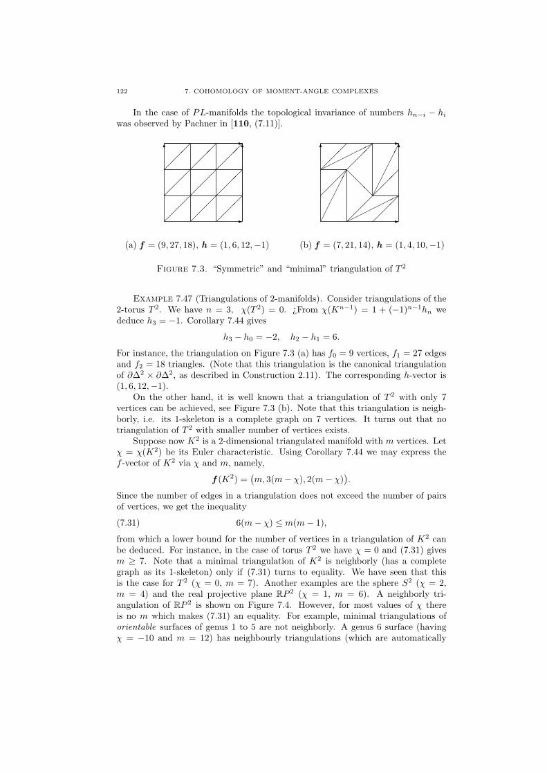
122 7. COHOMOLOGY OF MOMENT-ANGLE COMPLEXES
In the case of PL-manifolds the topological invariance of numbers hn−i − hi
was observed by Pachner in [110, (7.11)].
-
6-
6
¡¡
¡
¡¡
¡¡
¡¡
¡¡
¡¡
¡¡
¡¡¡
¡¡
¡¡
¡¡
¡¡
¡
(a) f = (9, 27, 18), h = (1, 6, 12,−1)
-
6-
6
¢¢¢¢¢¢
¡¡
¡¡
¡¡
©©©©©©
¡¡
¡
@@
@
¡¡
¡¡
¡¡
©©©©©©
¡¡
¡¢¢¢¢¢¢
(b) f = (7, 21, 14), h = (1, 4, 10,−1)
Figure 7.3. “Symmetric” and “minimal” triangulation of T 2
Example 7.47 (Triangulations of 2-manifolds). Consider triangulations of the2-torus T 2. We have n = 3, χ(T 2) = 0. ¿From χ(Kn−1) = 1 + (−1)n−1hn wededuce h3 = −1. Corollary 7.44 gives
h3 − h0 = −2, h2 − h1 = 6.
For instance, the triangulation on Figure 7.3 (a) has f0 = 9 vertices, f1 = 27 edgesand f2 = 18 triangles. (Note that this triangulation is the canonical triangulationof ∂∆2 × ∂∆2, as described in Construction 2.11). The corresponding h-vector is(1, 6, 12,−1).
On the other hand, it is well known that a triangulation of T 2 with only 7vertices can be achieved, see Figure 7.3 (b). Note that this triangulation is neigh-borly, i.e. its 1-skeleton is a complete graph on 7 vertices. It turns out that notriangulation of T 2 with smaller number of vertices exists.
Suppose now K2 is a 2-dimensional triangulated manifold with m vertices. Letχ = χ(K2) be its Euler characteristic. Using Corollary 7.44 we may express thef -vector of K2 via χ and m, namely,
f (K2) =(m, 3(m− χ), 2(m− χ)
).
Since the number of edges in a triangulation does not exceed the number of pairsof vertices, we get the inequality
(7.31) 6(m− χ) ≤ m(m− 1),
from which a lower bound for the number of vertices in a triangulation of K2 canbe deduced. For instance, in the case of torus T 2 we have χ = 0 and (7.31) givesm ≥ 7. Note that a minimal triangulation of K2 is neighborly (has a completegraph as its 1-skeleton) only if (7.31) turns to equality. We have seen that thisis the case for T 2 (χ = 0, m = 7). Another examples are the sphere S2 (χ = 2,m = 4) and the real projective plane RP 2 (χ = 1, m = 6). A neighborly tri-angulation of RP 2 is shown on Figure 7.4. However, for most values of χ thereis no m which makes (7.31) an equality. For example, minimal triangulations oforientable surfaces of genus 1 to 5 are not neighborly. A genus 6 surface (havingχ = −10 and m = 12) has neighbourly triangulations (which are automatically
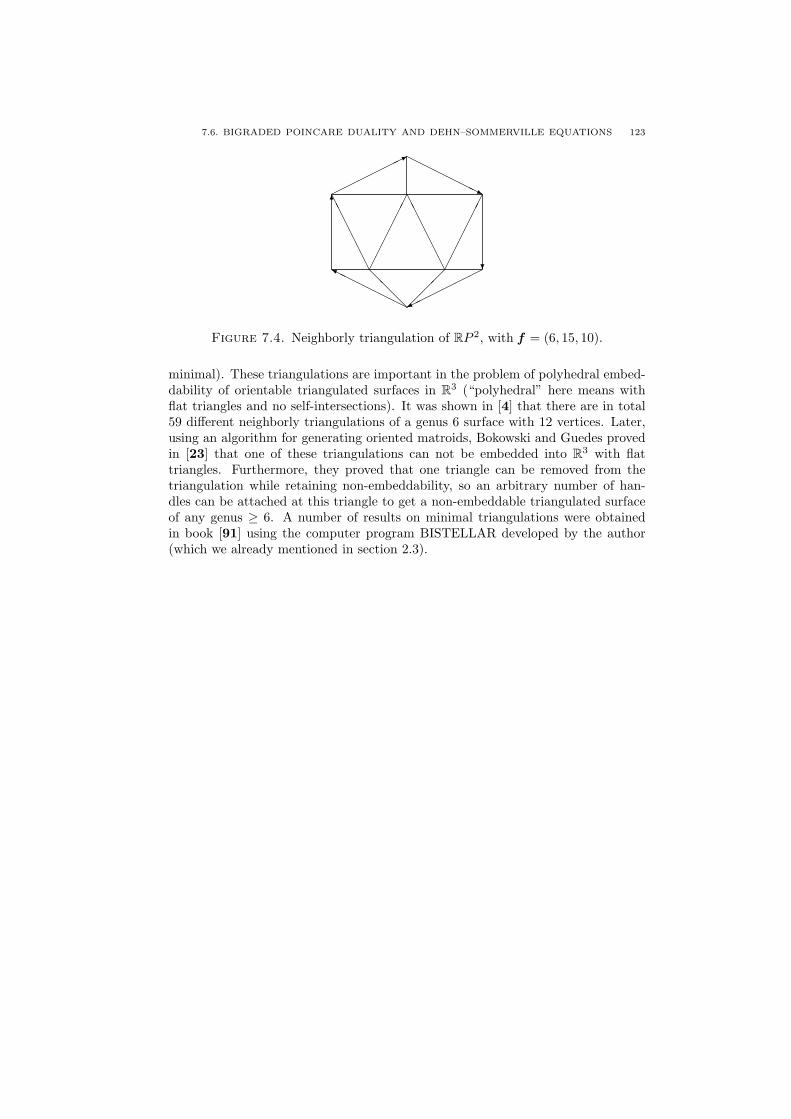
7.6. BIGRADED POINCARE DUALITY AND DEHN–SOMMERVILLE EQUATIONS 123
HHHHHHY
6©©©©©©*HHHHHHj
?©©©©©©¼@@
@
¡¡
¡A
AA
AA
A
¢¢¢¢¢¢
AA
AA
AA
¢¢¢¢¢¢
Figure 7.4. Neighborly triangulation of RP 2, with f = (6, 15, 10).
minimal). These triangulations are important in the problem of polyhedral embed-dability of orientable triangulated surfaces in R3 (“polyhedral” here means withflat triangles and no self-intersections). It was shown in [4] that there are in total59 different neighborly triangulations of a genus 6 surface with 12 vertices. Later,using an algorithm for generating oriented matroids, Bokowski and Guedes provedin [23] that one of these triangulations can not be embedded into R3 with flattriangles. Furthermore, they proved that one triangle can be removed from thetriangulation while retaining non-embeddability, so an arbitrary number of han-dles can be attached at this triangle to get a non-embeddable triangulated surfaceof any genus ≥ 6. A number of results on minimal triangulations were obtainedin book [91] using the computer program BISTELLAR developed by the author(which we already mentioned in section 2.3).

CHAPTER 8
Cohomology rings of subspace arrangementcomplements
8.1. General arrangements and their complements
Definition 8.1. An arrangement is a finite set A = L1, . . . , Lr of affinesubspaces in some affine space (either real or complex). An arrangement A is calleda subspace arrangement (or central arrangement) if all its subspaces are linear (i.e.,contain 0). Given an arrangement A = L1, . . . , Lr in Cm, define its support (orunion) |A| as
|A| :=r⋃
i=1
Li ⊂ Cm,
and its complement U(A) as
U(A) := Cm \ |A|,and similarly for arrangements in Rm.
Let A = L1, . . . , Lr be an arrangement. The intersections
v = Li1 ∩ · · · ∩ Lik
form a poset (L, <) with respect to the inclusion, called the intersection poset ofthe arrangement. The poset L is assumed to have a unique maximal element Tcorresponding to the ambient space of the arrangement. The rank function d on Lis defined by d(v) = dim v. The complex ord(L) (see Example 2.17) is called theorder complex of arrangement A. Define intervals
L(v,w) = x ∈ L : v < x < w, L>v = x ∈ L : x > v.Arrangements and their complements play a pivotal role in many construc-
tions of combinatorics, algebraic and symplectic geometry etc.; they also arise asconfiguration spaces for different classical mechanical systems. In the study of ar-rangements it is very important to get a sufficiently detailed description of thetopology of complements U(A) (this includes number of connected components,homotopy type, homology groups, cohomology ring etc.). A host of elegant resultsin this direction appeared during the last three decades, however, the whole pictureis far from being complete. The theory ascends to work of Arnold [6], in whichthe classifying space for the colored braid group is described as the complementof the arrangement of all diagonal hyperplanes zi = zj, 1 ≤ i < j ≤ n, in Cn.The latter complement can be thought as the configuration space of n orderedpoints in C. Its cohomology ring was also calculated in [6]. This result was gen-eralized by Brieskorn [29] and motivated the further development of the theory ofcomplex hyperplane arrangements (i.e. arrangements of codimension-one complexaffine subspaces). One of the main results here is the following.
125
126 8. COHOMOLOGY RINGS OF SUBSPACE ARRANGEMENT COMPLEMENTS
Theorem 8.2 ([6], [29]). Let A = L1, . . . , Lr be an arrangement of complexhyperplanes in Cm, where the hyperplane Lj is the zero set of linear function lj,j = 1, . . . , r. Then the integer cohomology algebra of the complement Cm \ |A| isisomorphic to the algebra generated by closed differential 1-forms 1
2πidljlj
.
Relations between the forms ωj = 12πi
dljlj
, j = 1, . . . , r, were explicitly describedby Orlik and Solomon [107]. We give their result in the central case, i.e. when allthe hyperplanes are vector subspaces. Then there is one relation
p∑
k=1
(−1)kωj1 ∧ · · · ∧ ωjk∧ · · · ∧ ωjp = 0,
for any minimal subset Lj1 , . . . , Ljp of hyperplanes of A such that codim Lj1 ∩
· · · ∩ Ljp= p− 1 (such subsets are called circuits of L).
Example 8.3. Let A be the arrangement of diagonal hyperplanes zj = zk,1 ≤ j < k ≤ n, in Cn. Then we have the forms ωjk = 1
2πid(zj−zk)
zj−zk, satisfying the
identitiesωij ∧ ωjk + ωjk ∧ ωki + ωki ∧ ωij = 0,
known as the Arnold relations.
The theory of complex hyperplane arrangements is probably the most well un-derstood part of the whole study. Several surveys and monographs are available; wemention just [108], [136] and [143], where further references can be found. Rela-tionships between real hyperplane arrangements, polytopes and oriented matroidsare discussed in [145, Lecture 7]. Another interesting related class of arrangementsis known as 2-arrangements in R2n. A 2-arrangement is an arrangement of realsubspaces of codimension 2 with even-dimension intersections. In particular, anycomplex hyperplane arrangement is a 2-arrangement. The relationships between2-arrangements and complex hyperplane arrangements are studied in [144].
In the case of general arrangement A, the celebrated Goresky–MacPhersontheorem [66, Part III] expresses the cohomology groups Hi(U(A)) (without ringstructure) as a sum of homology groups of subcomplexes of a certain simplicialcomplex.
Theorem 8.4 (Goresky and MacPherson [66, Part III]). The (co)homology ofa subspace arrangement complement U(A) in Rn: is given by
Hi
(U(A);Z
)=
⊕
v∈PHn−d(v)−i−1
(ord(L>v), ord(L(v,T ));Z
);
Hi(U(A);Z
)=
⊕
v∈PHn−d(v)−i−1
(ord(L>v), ord(L(v,T ));Z
),
(see Definition 8.1), where we assume that H−1(∅,∅) = H−1(∅,∅) = Z.
The original proof of this theorem used the stratified Morse theory , developedin [66].
Remark. Observing that ord(L>v) is the cone over ord(L(v,T )), we may rewritethe formula from Theorem 8.4 as
(8.1) Hi
(U(A);Z
)=
⊕
v∈PHn−d(v)−i−2
(ord(L(v,T ));Z
),
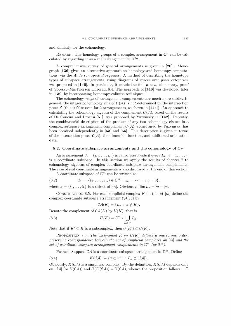
8.2. COORDINATE SUBSPACE ARRANGEMENTS 127
and similarly for the cohomology.
Remark. The homology groups of a complex arrangement in Cn can be cal-culated by regarding it as a real arrangement in R2n.
A comprehensive survey of general arrangements is given in [20]. Mono-graph [136] gives an alternative approach to homology and homotopy computa-tions, via the Anderson spectral sequence. A method of describing the homotopytypes of subspace arrangements, using diagrams of spaces over poset categories,was proposed in [146]. In particular, it enabled to find a new, elementary, proofof Goresky–MacPherson Theorem 8.4. The approach of [146] was developed laterin [139] by incorporating homotopy colimits techniques.
The cohomology rings of arrangement complements are much more subtle. Ingeneral, the integer cohomology ring of U(A) is not determined by the intersectionposet L (this is false even for 2-arrangements, as shown in [144]). An approach tocalculating the cohomology algebra of the complement U(A), based on the resultsof De Concini and Procesi [51], was proposed by Yuzvinsky in [142]. Recently,the combinatorial description of the product of any two cohomology classes in acomplex subspace arrangement complement U(A), conjectured by Yuzvinsky, hasbeen obtained independently in [53] and [55]. This description is given in termsof the intersection poset L(A), the dimension function, and additional orientationdata.
8.2. Coordinate subspace arrangements and the cohomology of ZK .
An arrangement A = L1, . . . , Lr is called coordinate if every Li, i = 1, . . . , r,is a coordinate subspace. In this section we apply the results of chapter 7 tocohomology algebras of complex coordinate subspace arrangement complements.The case of real coordinate arrangements is also discussed at the end of this section.
A coordinate subspace of Cm can be written as
(8.2) Lσ = (z1, . . . , zm) ∈ Cm : zi1 = · · · = zik= 0,
where σ = i1, . . . , ik is a subset of [m]. Obviously, dimLσ = m− |σ|.Construction 8.5. For each simplicial complex K on the set [m] define the
complex coordinate subspace arrangement CA(K) by
CA(K) = Lσ : σ /∈ K.Denote the complement of CA(K) by U(K), that is
(8.3) U(K) = Cm \⋃
σ/∈K
Lσ.
Note that if K ′ ⊂ K is a subcomplex, then U(K ′) ⊂ U(K).
Proposition 8.6. The assignment K 7→ U(K) defines a one-to-one order-preserving correspondence between the set of simplicial complexes on [m] and theset of coordinate subspace arrangement complements in Cm (or Rm).
Proof. Suppose CA is a coordinate subspace arrangement in Cm. Define
(8.4) K(CA) := σ ⊂ [m] : Lσ 6⊂ |CA|.Obviously, K(CA) is a simplicial complex. By the definition, K(CA) depends onlyon |CA| (or U(CA)) and U(K(CA)) = U(CA), whence the proposition follows. ¤
128 8. COHOMOLOGY RINGS OF SUBSPACE ARRANGEMENT COMPLEMENTS
If CA contains a hyperplane, say zi = 0, then its complement U(CA) isfactored as U(CA0) × C∗, where CA0 is a coordinate subspace arrangement inthe hyperplane zi = 0 and C∗ = C \ 0. Thus, for any coordinate subspacearrangement CA, the complement U(CA) decomposes as
U(CA) = U(CA′)× (C∗)k,
were CA′ is a coordinate arrangement in Cm−k that does not contain hyperplanes.On the other hand, (8.4) shows that CA contains the hyperplane zi = 0 if andonly if i is not a vertex of K(CA). It follows that U(K) is the complement of acoordinate arrangement without hyperplanes if and only if the vertex set of K is thewhole [m]. Keeping in mind these remarks, we restrict our attention to coordinatesubspace arrangements without hyperplanes and simplicial complexes on the vertexset [m].
Remark. In the notations of Construction 6.38 we have U(K) = K•(C,C∗).
Example 8.7. 1. If K = ∆m−1 then U(K) = Cm.2. If K = ∂∆m−1 (boundary of simplex) then U(K) = Cm \ 0.3. If K is a disjoint union of m vertices, then U(K) is the complement in Cm
of the set of all codimension-two coordinate subspaces zi = zj = 0, 1 ≤ i < j ≤ m.
The diagonal action of algebraic torus (C∗)m on Cm descends to U(K). Inparticular, there is the standard action of Tm on U(K). The quotient U(K)/Tm
can be identified with U(K) ∩ Rm+ , where Rm
+ is regarded as a subset of Cm.
Lemma 8.8. cc(K) ⊂ U(K) ∩ Rm+ and ZK ⊂ U(K) (see Construction 4.9
and (6.3)).
Proof. Take y = (y1, . . . , ym) ∈ cc(K). Let σ = i1, . . . , ik be the set of zerocoordinates of y, i.e. the maximal subset of [m] such that y ∈ Lσ ∩ Rn
+. Then itfollows from the definition of cc(K) (see (4.4)) that σ is a simplex of K. Hence,Lσ /∈ CA(K) and y ∈ U(K), which implies the first statement. The second assertionfollows from the fact that cc(K) is the quotient of ZK . ¤
Theorem 8.9. There is an equivariant deformation retraction U(K) → ZK .
Proof. First, we construct a deformation retraction r : U(K)∩Rm+ → cc(K).
This is done inductively. We start from the boundary complex of an (m−1)-simplexand remove simplices of positive dimensions until we obtain K. On each step weconstruct a deformation retraction, and the composite map will be the requiredretraction r.
If K = ∂∆m−1 is the boundary complex of an (m − 1)-simplex, then U(K) ∩Rm
+ = Rm+ \ 0. In this case the retraction r is shown on Figure 8.1. Now suppose
that K is obtained from K ′ by removing one (k − 1)-dimensional simplex τ =j1, . . . , jk, that is K ∪ τ = K ′. By the inductive hypothesis, we may assume thatthere is a deformation retraction r′ : U(K ′) ∩ Rm
+ → cc(K ′). Let a ∈ Rm+ be the
point with coordinates yj1 = . . . = yjk= 0 and yi = 1 for i /∈ τ . Since τ is not
a simplex of K, we have a /∈ U(K) ∩ Rm+ . At the same time, a ∈ Cτ (see (4.1)).
Hence, we can apply the retraction shown on Figure 8.1 on the face Cτ ⊂ Im,with center at a. Denote this retraction by rτ . Then r = rτ r′ is the requireddeformation retraction.
The deformation retraction r : U(K)∩Rm+ → cc(K) is covered by an equivariant
deformation retraction U(K) → ZK , which concludes the proof. ¤
8.2. COORDINATE SUBSPACE ARRANGEMENTS 129
e u
u u
-»»»»»»»:»»»»»»»»»»
©©©©©©©*
©©©©©©©©©©
½½
½½
½½
½>
½½
½½
½½
½½
½½
¡¡
¡¡
¡¡
¡µ
¡¡
¡¡
¡¡
¡¡
¡¡
6
¤¤¤¤¤¤¤º
¤¤¤¤¤¤¤¤¤¤
¢¢¢¢¢¢¢
¢¢¢¢¢¢¢¢¢¢
¶¶
¶¶
¶¶¶7
¶¶
¶¶
¶¶
¶¶
¶¶
Figure 8.1. The retraction r : U(K) ∩ Rm+ → cc(K) for K = ∂∆m−1.
In the case K = KP (i.e. K is a polytopal simplicial sphere corresponding toa simple polytope Pn) the deformation retraction U(KP ) → ZP from Theorem 8.9can be realized as the orbit map for an action of a contractible group. We denoteU(Pn) := U(KP ). Set
Rm> = (y1, . . . , ym) ∈ Rm : yi > 0, i = 1, . . . , m ⊂ Rm
+ .
Then Rm> is a group with respect to the multiplication, and it acts on Rm, Cm and
U(Pn) by coordinatewise multiplications. There is the isomorphism exp : Rm →Rm
> between the additive and the multiplicative groups taking (y1, . . . , ym) ∈ Rm
to (ey1 , . . . , eym) ∈ Rm> .
Let us consider the m× (m− n)-matrix W introduced in Construction 1.8 forevery simple polytope (1.1).
Proposition 8.10. For any vertex v = Fi1∩· · ·∩Fin of Pn the maximal minorWi1...in
of W obtained by deleting n rows i1, . . . , in is non-degenerate: detWi1...in6=
0.
Proof. If det Wi1...in= 0 then the vectors l i1 , . . . , l in (see (1.1)) are linearly
dependent, which is impossible. ¤
The matrix W defines the subgroup
(8.5) RW =(ew11τ1+···+w1,m−nτm−n , . . . , ewm1τ1+···+wm,m−nτm−n)
⊂ Rm> ,
where (τ1, . . . , τm−n) is running through Rm−n. Obviously, RW∼= Rm−n
> .
Theorem 8.11 ([33, Theorem 2.3] and [38, §3]). The subgroup RW acts freelyon U(Pn) ⊂ Cm. The composition ZP → U(Pn) → U(Pn)/RW of the embeddingie (Lemma 6.6) and the orbit map is an equivariant diffeomorphism (with respectto the corresponding Tm-actions).
Suppose now that Pn is a lattice simple polytope, and let MP be the corre-sponding toric variety (Construction 5.4). Along with the real subgroup RW ⊂Rm
> (8.5) define its complex analogue
CW =(ew11φ1+···+w1,m−nφm−n , . . . , ewm1φ1+···+wm,m−nφm−n)
⊂ (C∗)m,
where (φ1, . . . , φm−n) is running through Cm−n. Obviously, CW∼= (C∗)m−n. It is
shown in [45] (see also [9], [16]) that CW acts freely on U(Pn) and the toric variety
130 8. COHOMOLOGY RINGS OF SUBSPACE ARRANGEMENT COMPLEMENTS
MP can be identified with the orbit space (or geometric quotient) U(Pn)/CW .Thus, we have the following commutative diagram:
(8.6)
U(Pn)RW
∼=Rm−n>−−−−−−−→ ZP
CW∼=(C∗)m−n
yyT m−n
MP MP .
Remark. It can be shown [45, Theorem 2.1] that any toric variety MΣ cor-responding to a fan Σ ⊂ Rn with m one-dimensional cones can be identified withthe universal categorical quotient U(CAΣ)/G, where U(CAΣ) a certain coordinatearrangement complement (determined by the fan Σ) and G ∼= (C∗)m−n. The cate-gorical quotient becomes the geometric quotient if and only if the fan Σ is simplicial.In this case U(CAΣ) = U(KΣ).
On the other hand, if the projective toric variety MP is non-singular then MP
is a symplectic manifold of dimension 2n, and the action of Tn on it is Hamiltonian(see e.g. [9] or [45, §4]). In this case the diagram (8.6) displays MP as the result of asymplectic reduction. Namely, let HW
∼= Tm−n be the maximal compact subgroupin CW , and µ : Cm → Rm−n the moment map for the Hamiltonian action of HW
on Cm. Then for any regular value a ∈ Rm−n of the map µ there is the followingdiffeomorphism:
µ−1(a)/HW −→ U(Pn)/CW = MP
(details can be found in [9]). In this situation µ−1(a) is exactly our manifold ZP .This gives us another interpretation of the manifold ZP as the level surface for themoment map (in the case when Pn can be realized as the quotient of a non-singularprojective toric variety).
Example 8.12. Let Pn = ∆n (the n-simplex). Then m = n + 1, U(Pn) =Cn+1 \ 0. Moreover, RW
∼= R>, CW∼= C∗ and HW
∼= S1 are the diagonalsubgroups in Rn+1
> , (C∗)n+1 and Tm+1 respectively (see Example 1.9). Hence,
ZP∼= S2n+1 =
(Cn+1 \ 0)/R>, MP =
(Cn+1 \ 0)/C∗ = CPn.
The moment map µ : Cm → R takes (z1, . . . , zm) ∈ Cm to 12 (|z1|2 + . . . + |zm|2),
and for a 6= 0 we have µ−1(a) ∼= S2n+1 ∼= ZK .
Now we have the following result for the cohomology of subspace arrangementcomplements.
Theorem 8.13. The following isomorphism of graded algebras holds:
H∗(U(K)) ∼= Tork[v1,...,vm]
(k(K),k
)
= H[Λ[u1, . . . , um]⊗ k(K), d
].
Proof. This follows from theorems 8.9, 7.6 and 7.7. ¤
Theorem 8.13 provides an effective way to calculate the cohomology algebraof the complement of any complex coordinate subspace arrangement. The Koszulcomplex was also used by De Concini and Procesi [51] and Yuzvinsky [142] forconstructing rational models of the cohomology algebra of an arrangement com-plement. As we see, in the case of coordinate subspace arrangements calculations
8.2. COORDINATE SUBSPACE ARRANGEMENTS 131
become shorter and more effective as soon as the Stanley–Reisner ring is broughtinto the picture.
Problem 8.14. Calculate the integer cohomology algebra of a coordinate sub-space arrangement complement and compare it with the corresponding Tor-algebraTorZ[v1,...,vm](Z(K),Z).
Example 8.15. Let K be a disjoint union of m vertices. Then U(K) is thecomplement to the set of all codimension-two coordinate subspaces zi = zj = 0,1 ≤ i < j ≤ m, in Cm (see Example 8.7). The face ring is k(K) = k[v1, . . . , vm]/IK ,where IK is generated by the monomials vivj , i 6= j. An easy calculation usingCorollary 8.13 shows that the subspace of cocycles in k(K) ⊗ Λ[u1, . . . , um] hasthe basis consisting of monomials vi1ui2ui3 · · ·uik
with k ≥ 2 and ip 6= iq forp 6= q. Since deg(vi1ui2ui3 · · ·uik
) = k+1, the space of (k+1)-dimensional cocycleshas dimension m
(m−1k−1
). The space of (k + 1)-dimensional coboundaries is
(mk
)-
dimensional (it is spanned by the coboundaries of the form d(ui1 · · ·uik)). Hence,
dim H0(U(K)
)= 1, H1
(U(K)
)= H2
(U(K)
)= 0,
dim Hk+1(U(K)
)= m
(m−1k−1
)− (mk
)= (k − 1)
(mk
), 2 ≤ k ≤ m,
and the multiplication in the cohomology is trivial.In particular, for m = 3 we have 6 three-dimensional cohomology classes [viuj ],
i 6= j, subject to 3 relations [viuj ] = [vjui], and 3 four-dimensional cohomologyclasses [v1u2u3], [v2u1u3], [v3u1u2] subject to one relation
[v1u2u3]− [v2u1u3] + [v3u1u2] = 0.
Hence, dim H3(U(K)) = 3, dimH4(U(K)) = 2, and the multiplication is trivial.It can be shown that U(K) in this case has a homotopy type of a wedge of spheres:
U(K) ' S3 ∨ S3 ∨ S3 ∨ S4 ∨ S4.
Example 8.16. Let K be the boundary of an m-gon, m > 3. Then
U(K) = Cm \⋃
i−j 6=0,1 mod m
zi = zj = 0.
By Theorem 8.13, the cohomology ring of H∗(U(K);k) is isomorphic to the ringdescribed in Example 7.22 (note that the multiplication is non-trivial here).
As it is shown in [65], in the case of arrangements of real coordinate subspacesonly additive analogue of our Theorem 8.13 holds. Namely, let us consider thepolynomial ring k[x1, . . . , xm] with deg xi = 1, i = 1, . . . , m. Then the gradedstructure in the face ring k(K) changes accordingly. The Betti numbers of thereal coordinate subspace arrangement UR(K) can be calculated by means of thefollowing result.
Theorem 8.17 ([65, Theorem 3.1]). The following isomorphism hold:
Hp(UR(K)
) ∼=∑
−i+j=p
Tor−i,jk[x1,...,xm]
(k(K),k
)= H−i,j
[Λ[u1, . . . , um]⊗ k(K), d
],
where bideg ui = (−1, 1), bideg vi = (0, 1), dui = xi, dxi = 0.
As it was observed in [65], there is no multiplicative isomorphism analogous toTheorem 8.13 in the case of real arrangements, that is, the algebras H∗(UR(K)) andTork[x1,...,xm](k(K),k) are not isomorphic in general. The paper [65] also contains
132 8. COHOMOLOGY RINGS OF SUBSPACE ARRANGEMENT COMPLEMENTS
the formulation of the first multiplicative isomorphism of our Theorem 8.13 forcomplex coordinate subspace arrangements (see [65, Theorem 3.6]), with referenceto a paper by Babson and Chan (unpublished).
Up to this point we have used the description of coordinate subspaces by meansof equations (see (8.2)). On the other hand, a coordinate subspace can be definedas the linear span of a subset of the standard basis e1, . . . , em. This leads tothe dual approach to coordinate subspace arrangements, which corresponds to thepassage from simplicial complex K to the dual complex K (Example 2.26). Namely,we have
CA(K) =spanei1 , . . . , eik
: i1, . . . , ik ∈ K
(see Construction 8.5). We may observe further that in the coordinate subspacearrangement case the intersection poset (L, <) is the inclusion poset of simplicesof K with added maximal element (or equivalently, the inclusion poset of cone K).Hence, ord(L(v,T )) is the barycentric subdivision of link bK v, where v is regarded asa simplex of K. Thus, we may rewrite the Goresky–MacPherson formula (8.1) inthe complex subspace arrangement case as
(8.7) Hi
(U(K)
)=
⊕
σ∈ bKH2m−2|σ|−i−2
(link bK σ
),
(note that d(σ) = |σ| and the dimensions are doubled since we are in the complexarrangement case).
The above observations were used in [54] to describe the product of two co-homology classes of a coordinate subspace arrangement complement (either real orcomplex) in terms of the combinatorics of links of simplices in K (see [54, Theo-rem 1.1]).
On the other hand, the isomorphism of algebras established in Theorem 8.13 al-lows to connect two seemingly unrelated results, namely, the Goresky–Macphersontheorem for the cohomology of an arrangement complement and the Hochster the-orem from the commutative algebra.
Proposition 8.18. After identification of the cohomology H∗(U(K)) with theTor-algebra Tork[v1,...,vm](k(K),k) established by Theorem 8.13, the Hochster The-orem 3.27 becomes equivalent to the Goresky–MacPherson Theorem 8.4 in the caseof coordinate subspace arrangements.
Proof. Using Theorem 8.13 to identify β−i,2j(k(K)) with dimk H−i,2j(U(K)),we get the following formula from Hochster’s Theorem 3.27:
Hp
(U(K)
)=
⊕
τ⊂[m]
Hp−|τ |−1(Kτ ).
Non-empty simplices τ ∈ K do not contribute to the above sum since the corre-sponding full subcomplexes Kτ are contractible. Since H−1(∅) = k, the emptysubset of [m] only contributes k to H0(U(K)). Hence, we may rewrite the aboveformula as
(8.8) Hp
(U(K)
)=
⊕
τ /∈K
Hp−|τ |−1(Kτ ).
Using the Alexander duality (Proposition 2.29), we calculate
Hp−|τ |−1(Kτ ) = Hm−3−p+|τ |+1−|bτ |(link bK τ)
= H2m−2|bτ |−p−2(link bK τ
),
8.3. DIAGONAL SUBSPACE ARRANGEMENTS 133
where τ = [m] \ τ is a simplex of K. Now we observe that (8.8) is equivalentto (8.7). ¤
8.3. Diagonal subspace arrangements and the cohomology of ΩZK .
Another interesting particular class of subspace arrangements is diagonal ar-rangements. A classical example of a diagonal subspace arrangement is given by thearrangement of all diagonal hyperplanes zi = zj in Cm, mentioned in section 8.1(see Example 8.3). Some further particular examples of diagonal arrangements, theso-called k-equal arrangements were considered, e.g. in [20], while the cohomologyof general diagonal arrangement complements was studied in [114]. In this sectionwe establish certain relationships between this cohomology and the cohomology ofthe loop spaces Ω(BTZK) (see section 6.5) and ΩZK .
Definition 8.19. For each subset σ = i1, . . . , ik ⊂ [m] define the diagonalsubspace Dσ in Rm by
Dσ = (y1, . . . , ym) ∈ Rm : yi1 = · · · = yik.
Diagonal subspaces in Cm are defined similarly. An arrangement A = L1, . . . , Lris called diagonal if all Li, i = 1, . . . , r, are diagonal subspaces.
Construction 8.20. Given a simplicial complex K on the vertex set [m],introduce the diagonal subspace arrangement DA(K) as the set of subspaces Dσ
such that σ is not a simplex of K:
DA(K) = Dσ : σ /∈ K.Denote the complement of the arrangement DA(K) by M(K).
The following statement is proved in the similar way as the correspondingstatement (Proposition 8.6) for coordinate subspace arrangements.
Proposition 8.21. The assignment K 7→ M(K) defines a one-to-one order-preserving correspondence between the set of simplicial complexes on the vertexset [m] and the set of diagonal subspace arrangement complements in Rm.
Here we still assume that k is a field. The multigraded (or Nm-graded) struc-ture in the ring k[v1, . . . , vm] (Construction 3.33) defines an Nm-grading in theStanley–Reisner ring k(K). The monomial vi1
1 · · · vimm acquires the multidegree
(2i1, . . . , 2im). Let us consider the modules Tork(K)(k,k). They can be calcu-lated by means of the minimal free resolution (Example 3.23) of k (regarded as ak(K)-module). The minimal resolution also carries a natural Nm-grading, and wedenote the subgroup of elements of multidegree (2i1, . . . , 2im) in Tork(K)(k,k) byTork(K)(k,k)(2i1,...,2im).
Theorem 8.22 ([114, Theorem 1.3]). The following isomorphism holds for thecohomology groups of a real diagonal subspace arrangement complement M(K):
Hi(M(K);k
) ∼= Tor−(m−i)k(K) (k,k)(2,...,2).
Remark. Instead of simplicial complexes K on the vertex set [m] the authorsof [114] considered square-free monomial ideals I ⊂ k[v1, . . . , vm]. Proposition 3.3shows that the two approaches are equivalent.
134 8. COHOMOLOGY RINGS OF SUBSPACE ARRANGEMENT COMPLEMENTS
Theorem 8.23. The following additive isomorphism holds:
H∗(Ω(BTZK);k) ∼= Tork(K)(k,k).
Proof. Let us consider the Eilenberg–Moore spectral sequence of the Serre fi-bration P → DJ (K) with fibre ΩDJ (K), where DJ (K) is the Davis–Januszkiewiczspace (Definition 6.27) and P is the path space over DJ (K). By Corollary 7.4,
(8.9) E2 = TorH∗(DJ(K))
(H∗(P ),k
) ∼= Tork(K)(k,k),
and the spectral sequence converges to TorC∗(DJ (K))(C∗(P ),k) ∼= H∗(ΩDJ (K)).
Since P is contractible, there is a cochain equivalence C∗(P ) ' k. We haveC∗(DJ (K)) ∼= k(K). Therefore,
TorC∗(DJ(K))
(C∗(P ),k
) ∼= Tork(K)(k,k),
which together with (8.9) shows that the spectral sequence collapses at the E2
term. Hence, H∗(ΩDJ (K)) ∼= Tork(K)(k,k). Finally, Theorem 6.29 shows thatH∗(ΩDJ (K)) ∼= H∗(ΩBTZK), which concludes the proof. ¤
Proposition 8.24. The following isomorphism of algebras holds
H∗(Ω(BTZK)) ∼= H∗(ΩZK)⊗ Λ[u1, . . . , um].
Proof. Consider the bundle BTZK → BTm with fibre ZK . It is easy to seethat the corresponding loop bundle ΩBTZK → Tm with fibre ΩZK is trivial (notethat ΩBTm ' Tm). To finish the proof it remains to mention that H∗(Tm) ∼=Λ[u1, . . . , um]. ¤
Theorems 8.9 and 8.13 give an application of the theory of moment-angle com-plexes to calculating the cohomology ring of a coordinate subspace arrangementcomplement. Likewise, theorems 8.22, 8.23 and Proposition 8.24 establish a con-nection between the cohomology of a diagonal subspace arrangement complementand the cohomology of the loop space over the moment-angle complex ZK . How-ever, the latter relationships are more subtle than those in the case of coordinatesubspace arrangements. For instance, we do not have an analogue of the multi-plicative isomorphism from Theorem 8.13. It would be very interesting to get anystatement of such kind, or discover other new applications of the theory of moment-angle complexes to diagonal (or maybe even general) subspace arrangements.
Bibliography
[1] J. F. Adams, On the cobar construction, Proc. Nat. Acad. Sci. USA 42 (1956), 409–412.[2] J. F. Adams, On the non-existence of elements of Hopf invariant one, Ann. of Math., II 72
(1960), no. 1, 20–104.[3] R. Adin, A new cubical h-vector, Discrete Math. 157 (1996), no. 1-3, 3–14.[4] A. Altshuler, J. Bokowski and P. Schuchert, Neighborly 2-manifolds with 12 vertices, J.
Comb. Theory, Ser. A 75 (1996), no. 1, 148–162.[5] S. Akbulut and J.D. McCarthy, Casson’s Invariant for Oriented Homology 3-spheres, Math.
Notes 36, Princeton Univ. Press, Princeton, N.J., 1990.[6] V. I. Arnold, The cohomology ring of the colored braid group (Russian), Mat. Zametki 5
(1969), 227–231; English translation in: Math. Notes 5 (1969), 138–140.[7] M. F. Atiyah and R. Bott, A Lefschetz fixed point formula for elliptic complexes: I, Annals
of Math. 86 (1967), no. 2, 374–407.[8] M. F. Atiyah and F. Hirzebruch, Spin-manifolds and group actions, in: Essays in Topology
and Related Topics, Springer-Verlag, Berlin-Heidelberg-New York, 1970, pp. 18–28.[9] M. Audin, The Topology of Torus Actions on Symplectic Manifolds, Progress in Mathemat-
ics 93, Birkhauser, Boston Basel Berlin, 1991.[10] E. Babson, L. Billera and C. Chan, Neighborly cubical spheres and a cubical lower bound
conjecture, Israel J. Math. 102 (1997), 297–315.[11] A. Bahri and M. Bendersky, The KO-theory of toric manifolds, Trans. Amer. Math. Soc.
352 (2000), no. 3, 1191–1202; http://xxx.lanl.gov/abs/math.AT/9904087.[12] D. Barnette, Diagrams and Schlegel diagrams, in: “Combinatorial Structures and Their
Applications” (Proc. Calgary Internat. Conference, Calgary 1969), Gordon and Breach,New York, 1970, pp. 1–4.
[13] D. Barnette, The minimum number of vertices of a simple polytope, Izrael J. Math. 10(1971), 121–125.
[14] D. Barnette, The triangulations of the 3-sphere with up to 8 vertices, J. CombinatorialTheory. Ser. A 14 (1973), 37–52.
[15] D. Barnette, A proof of the lower bound conjecture for convex polytopes, Pacific J. Math.46 (1973), 349–354.
[16] V.V. Batyrev, Quantum Cohomology Rings of Toric Manifolds, Journees de GeometrieAlgebrique d’Orsay (Juillet 1992), Asterisque 218, Societe Mathematique de France, Paris,1993, pp. 9–34; http://xxx.lanl.gov/abs/alg-geom/9310004.
[17] M. Bayer and L. Billera, Generalized Dehn–Sommerville relations for polytopes, spheres andEulerian partially ordered sets, Invent. Math. 79 (1985), 143–157.
[18] L. Billera and C. Lee, Sufficiency of McMullen’s conditions for f-vectors of simplicial poly-topes, Bull. Amer. Math. Soc. 2 (1980), 181–185.
[19] L. Billera and C. Lee, A proof of the sufficiency of McMullen’s conditions for f-vectors ofsimplicial polytopes, J. Comb. Theory, Ser. A 31 (1981), 237–255.
[20] A. Bjorner, Subspace arrangements, in: Proc. of the First European Congress of Mathemat-ics (Paris 1992), A. Joseph et al., eds., Progress in Mathematics 119, Birkhauser, Basel,1994, Vol. 1, pp. 321–370.
[21] A. Bjorner and F. Lutz, Simplicial manifolds, bistellar flips and 16-vertex triangulation ofthe Poincare homology 3-sphere, Experiment. Math. 9 (2000), no. 2, 275–289.
[22] A. Bjorner and G.M. Ziegler, Combinatorial stratification of complex arrangements, J.Amer. Math. Soc. 5 (1992), no. 1, 105–149.
[23] J. Bokowski and A. Guedes de Oliveira, On the generation of oriented matroids, DiscreteComput. Geom. 24 (2000), no. 2–3, 197–208.
135
136 BIBLIOGRAPHY
[24] A.K. Bousfield and D.M. Kan, Homotopy limits, completions and localizations, LectureNotes in Mathematics 304, Springer-Verlag, Berlin–New York, 1972.
[25] C. Boyer, K. Galicki, B. Mann and E. Rees, Compact 3-Sasakian 7-manifolds with arbitrarysecond Betti number, Invent. Math. 131 (1998), 321–344.
[26] G. E. Bredon, Introduction to compact transformation groups, Academic Press, New York–London, 1972.
[27] P. Bressler and V. Lunts, Intersection cohomology on nonrational polytopes, preprint (2000),arXiv: math.AG/0002006.
[28] E. Brieskorn, Sur les groupes de tresses (d’apres V. I. Arnol’d), in: Seminaire Bourbaki1971/72, Lecture Notes in Math. 317, Springer-Verlag, Berlin-New York, 1973, pp. 21–44.
[29] A. Brønsted, An Introduction to Convex Polytopes, Graduate Texts in Math. 90, Springer-Verlag, New-York, 1983.
[30] V.M. Bukhshtaber and T.E. Panov, Algebraic topology of manifolds defined by simple poly-topes (Russian), Uspekhi Mat. Nauk 53 (1998), no. 3, 195–196; English translation in:Russian Math. Surveys 53 (1998), no. 3, 623–625.
[31] V.M. Buchstaber and T. E. Panov. Torus actions and combinatorics of polytopes (Russian),Tr. Mat. Inst. Steklova 225 (1999), 96–131; English translation in: Proc. Steklov Inst. Math.1999, no. 2 (225), 87–120; arXiv: math.AT/9909166.
[32] V.M. Buchstaber and T.E. Panov, Torus actions, equivariant moment-angle complexes andcoordinate subspace arrangements (Russian), in: “Representation theory, dynamical sys-tems, combinatorical and algorithmic methods”, Part 5, A.M. Vershik, ed., Zap. Nauchn.Sem. S.-Peterburg. Otdel. Mat. Inst. Steklov. (POMI) 266, 2000, pp. 29–50; English trans-lation in: Journal of Math. Sciences, to appear; arXiv: math.AT/9912199.
[33] V.M. Buchstaber and T.E. Panov. Torus actions determined by simple polytopes, in: Ge-ometry and Topology: Aarhus, K. Grove, I. Madsen, and E. Pedersen, eds., Contemp. Math.258, Amer. Math. Soc., Providence, R.I., 2000, pp. 33–46.
[34] V.M. Buchstaber and T.E. Panov. Moment-angle complexes and combinatorics of simplicialmanifolds (Russian), Uspekhi Mat. Nauk 55 (2000), no. 3, 171–172; English translation in:Russian Math. Surveys 55 (2000), no. 3, 567–569.
[35] V.M. Buchstaber and T.E. Panov. Torus actions, combinatorial topology and homologicalalgebra (Russian), Uspekhi Mat. Nauk 55 (2000), no. 5, 3–106; English translation in:Russian Math. Surveys 55 (2000), no. 5, 825–921; arXiv: math.AT/0010073.
[36] V.M. Buchstaber and N. Ray, Flag manifolds and the Landweber–Novikov algebra, Geom.Topol. 2 (1998), 79–101; arXiv: math.AT/9806168; http://www.maths.warwick.ac.uk/gt/.
[37] V.M. Bukhshtaber and N. Ray, Toric manifolds and complex cobordisms (Russian), UspekhiMat. Nauk 53 (1998), no. 2, 139–140; English translation in: Russian Math. Surveys 53(1998), no. 2, 371–373.
[38] V.M. Buchstaber and N. Ray, Tangential structures on toric manifolds, and connected sumsof polytopes, Internat. Math. Res. Notices 2001, no. 4, 193–219; arXiv: math.AT/0010025.
[39] J.W. Cannon, Shrinking cell-like decompositions of manifolds. Codimension three., Ann. ofMath., II 110 (1979), no. 1, 83–112.
[40] H. Cartan and S. Eilenberg, Homological Algebra, Princeton Univ. Press, Princeton, N.J.,1956.
[41] R. Charney and M. Davis, The Euler characteristic of a nonpositively curved, piecewiseEuclidean manifold, Pacific J. Math. 171 (1995), no. 1, 117–137.
[42] B. Chen and M. Yan, Singularity from Eulerian viewpoint, Proc. Steklov Inst. Math. 1998,no. 2 (221), 296–311.
[43] I.M. Chiswell, The Euler characteristic of graph products and of Coxeter groups, in: Dis-crete groups and geometry (Birmingham, 1991), London Math. Soc. Lecture Note Ser. 173,Cambridge Univ. Press, Cambridge, 1992, pp. 36–46.
[44] P. E. Conner and E.E. Floyd, Differentiable periodic maps, Springer-Verlag, Berlin, 1964.[45] D.A. Cox, Recent developments in toric geometry, Proc. Symp. Pure Math. 62, Part 2,
Amer. Math. Soc., Providence, R.I., 1997, pp. 389–436; arXiv: alg-geom/9606016.[46] V. Danilov, The geometry of toric varieties (Russian), Uspekhi Mat. Nauk 33 (1978), no. 2,
85–134; English translation in: Russian Math. Surveys 33 (1978), no. 2, 97–154.[47] M. Davis, Groups generated by reflections and aspherical manifolds not covered by Euclidean
space, Ann. of Math. 117 (1983), 293–324.
BIBLIOGRAPHY 137
[48] M. Davis and T. Januszkiewicz, Convex polytopes, Coxeter orbifolds and torus actions, DukeMath. J. 62 (1991), no. 2, 417–451.
[49] M. Davis and T. Januszkiewicz, Right-angled Artin groups are commensurable with right-angled Coxeter groups, J. Pure Appl. Algebra 153 (2000), no. 3, 229–235.
[50] M. Davis and B. Okun, Vanishing theorems and conjectures for the `2-homology ofright-angled Coxeter groups, Geom. Topol. 5 (2001), 7–74; arXiv: math.GR/0102104;http://www.maths.warwick.ac.uk/gt/.
[51] C. De Concini and C. Procesi, Wonderful models of subspace arrangements, Selecta Math.,New Ser. 1 (1995), no. 3, 459–494.
[52] M. Dehn, Die Eulersche Formel im Zusammenhang mit dem Inhalt in der nicht-Euklidischen Geometrie, Math. Ann. 61 (1905), 561–568.
[53] P. Deligne, M. Goresky and R. MacPherson, L’algebre de cohomologie du complement, dansun espace affine, d’une famille finie de sous-espaces affines, Michigan Math. J. 48 (2000),121–136.
[54] M. De Longueville, The ring structure on the cohomology of coordinate subspace arrange-ments, Math. Z. 233 (2000), no. 3, 553–577.
[55] M. de Longueville and C.A. Schultz, The cohomology rings of complements of subspacearrangements, Math. Ann. 319 (2001), no. 4, 625–646.
[56] N. Dobrinskaya, The classification problem for quasitoric manifolds over given simple poly-tope (Russian), Funktsional. Anal. i Prilozhen. 35 (2001), no. 2, 3–11; English translationin: Funct. Anal. and Appl. 35 (2001), no. 2.
[57] N. P. Dolbilin, M.A. Shtan’ko and M. I. Shtogrin, Cubic subcomplexes in regular lattices(Russian), Dokl. Akad. Nauk SSSR 291 (1986), no. 2, 277–279; English translation in: Sov.Math., Dokl. 34 (1987), no. 3, 467–469.
[58] R.D. Edwards, The double suspension of a certain homology 3-sphere is S5., Notices AMS22, A-334 (1975).
[59] R.D. Edwards, The topology of manifolds and cell-like maps, in: Proceedings of the Inter-national Congress of Mathematicians (Helsinki, 1978), Acad. Sci. Fennica, Helsinki, 1980,pp. 111–127.
[60] S. Eilenberg and J.C. Moore, Homology and fibrations. I, Comment. Math. Helv. 40 (1966),199–236.
[61] G. Ewald, Combinatorial Convexity and Algebraic Geometry, Graduate Texts in Math. 168,Springer-Verlag, New-York, 1996.
[62] S. Fischli and D. Yavin, Which 4-manifolds are toric varieties?, Math. Z. 215 (1994), no. 2,179–185.
[63] M.H. Freedman and F. Quinn, Topology of 4-manifolds, Princeton Mathematical Series 39,Princeton Univ. Press, Princeton, N.J., 1990.
[64] W. Fulton, Introduction to Toric Varieties, Ann. of Math. Studies 131, Princeton Univ.Press, Princeton, N.J., 1993.
[65] V. Gasharov, I. Peeva and V. Welker, Coordinate subspace arrange-ments and monomial ideals, preprint, 1999; Proceedings of the Os-aka Meeting on Combinatorics and Commutative Algebra, to appear;http://www.mathematik.uni-marburg.de/~welker/sections/preprints.html.
[66] M. Goresky and R. MacPherson, Stratified Morse Theory, Springer-Verlag, Berlin–NewYork, 1988.
[67] J. Gretenkort, P. Kleinschmidt and B. Sturmfels, On the existence of certain smooth toricvarieties, Discrete Comput. Geom. 5 (1990), no. 3, 255–262.
[68] M. Gromov, Hyperbolic groups, in: Essays in Group Theory, S.M. Gersten, ed., Math. Sci.Res. Inst. Publ. 8, Springer-Verlag, New York, 1987, pp. 75–263.
[69] B. Grunbaum, Convex Polytopes, Interscience Publishers John Wiley & Sons, Inc., London–New York–Sydney, 1967.
[70] B. Grunbaum and V.P. Sreedharan, An enumeration of simplicial 4-polytopes with 8 ver-tices, J. Combinatorial Theory 2 (1967), 437–465.
[71] A. Hattori, Almost complex toric manifolds and positive line bundles, in: Homotopy andGeometry (Warsaw, 1997), Banach Center of Publications, vol. 45, Polish Acad. of Sci.,Warsaw, 1998, pp. 95–114.
[72] A. Hattori and M. Masuda, Theory of multi-fans, preprint (2001), arXiv: math.SG/0106229.
138 BIBLIOGRAPHY
[73] A. Hattori and M. Masuda, Elliptic genera, torus manifolds and multi-fans, preprint (2001),arXiv: math.SG/0107014.
[74] F. Hirzebruch, Topological methods in algebraic geometry, 3rd edition, with appendices byR. L. E. Schwarzenberger an A. Borel, Springer-Verlag, Berlin–Heidelberg, 1966.
[75] F. Hirzebruch, T. Berger and R. Jung, Manifolds and Modular Forms, Second Edition, APublication from the Max-Planc-Institut fur Mathematik, Bonn, 1994.
[76] M. Hochster, Cohen–Macaulay rings, combinatorics, and simplicial complexes, in: RingTheory II (Proc. Second Oklahoma Conference), B.R. McDonald and R. Morris, eds.,Dekker, New York, 1977, pp. 171–223.
[77] P. Hudson, Piecewise Linear Topology, W. A. Benjamin, Inc., New York–Amsterdam, 1969.[78] I. Izmest’ev, Manifolds determined by simple polyhedra as configuration spaces of hinge
mechanisms (Russian), Uspekhi Mat. Nauk 55 (2000), no. 1, 185–186; English translationin: Russian Math. Surveys 55 (2000), no. 1, 176–177.
[79] I. Izmest’ev, 3-dimensional manifolds defined by simple polytopes with coloured facets (Rus-sian), Mat. Zametki 69 (2001), no. 3, 375–382; English translation in: Math. Notes 69(2001), no. 3.
[80] K. Janich, On the classification of O(n)-manifolds, Math. Ann. 176 (1968), 53–76.[81] M. Joswig, Projectivities in Simplicial Complexes and Colorings of Simple Polytopes,
preprint (2001), arXiv: math.CO/0102186.[82] J. Jurkiewicz, Torus embeddings, polyhedra, k∗-actions and homology, Dissertationes Math.
(Rozprawy Mat.) 236 (1985).[83] G. Kalai, Rigidity and the lower bound Theorem. I, Inv. Math. 88 (1987), no. 1, 125–151.[84] A.G. Khovanskii, Hyperplane sections of polyhedra, toric varieties and discrete groups in
Lobachevskii space (Russian), Funktsional. Anal. i Prilozhen. 20 (1986), no. 1, 50–61; Eng-lish translation in: Funct. Anal. Appl. 20 (1986), no. 1, 41–50.
[85] R.C. Kirby and L.C. Siebenmann, Foundational Essays on Topological Manifolds, Smooth-ings, and Triangulations, Ann. of Math. Stud. 88, Princeton Univ. Press, Princeton, N.J.,1977.
[86] V. Klee, A combinatorial analogue of Poincare’s duality theorem, Canad. J. Math. 16(1964), 517–531.
[87] V. Klee and P. Kleinschmidt, Convex polytopes and related complexes, in: Handbook ofCombinatorics. Vol. 1,2, R. L. Graham et al, eds., Elsevier Science B.V., Amsterdam, 1995,pp. 875–917.
[88] P. Kleinschmidt, A classification of toric varieties with few generators, Aequationes Math.35 (1988), no. 2–3, 254–266.
[89] P. S. Landweber, Homological properties of comodules over MU∗(MU) and BP∗(BP ),Amer. J. Math. 98 (1976), no. 3, 591–610.
[90] N.C. Leung and V. Reiner, The signature of a toric variety, preprint, 1999;http://www.math.umn.edu/~reiner/Papers/papers.html.
[91] F. H. Lutz, Triangulated Manifolds with Few Vertices (with additional contributions byA. Borner, E. Kohler, and W. Kuhnel), in preparation.
[92] S. Maclane, Homology, Springer-Verlag, Berlin, 1963.[93] M. Masuda, Unitary toric manifolds, multi-fans and equivariant index, Tohoku Math. J.
51 (1999), no. 2, 237–265.[94] P. Mani, Spheres with few vertices, J. Combinatorial Theory. Ser. A 13 (1972), 346–352.[95] P. McMullen, The maximum numbers of faces of a convex polytope, Mathematika 17 (1970),
179–184.[96] P. McMullen, The numbers of faces of simplicial polytopes, Israel J. Math. 9 (1971), 559–570.[97] P. McMullen, On simple polytopes, Invent. Math. 113 (1993), no. 2, 419–444.[98] P. McMullen, Weights on polytopes, Discrete Comput. Geom. 15 (1996), no. 4, 363–388.[99] P. McMullen and G. Shephard, Convex Polytopes and the Upper Bound Conjecture, London
Maht. Soc. Lecture Notes Series 3, Cambridge University Press, Cambridge, 1971.[100] P. McMullen and D.W. Walkup A generalised lower bound conjecture for simplicial poly-
topes, Mathematika 18 (1971), 264–273.[101] E. E. Moise, Geometric Topology in Dimensions 2 and 3, Graduate Texts in Math. 47,
Springer-Verlag, New-York, 1977.[102] R. Morelli, The birational geometry of toric varieties, J. Algebr. Geom. 5 (1996), no. 4,
751-782.
BIBLIOGRAPHY 139
[103] A. Nabutovsky, Geometry of the space of triangulations of a compact manifold, Comm.Math. Phys. 181 (1996), no. 2, 303–330.
[104] S. P. Novikov. Topology I, Encyclopaedia Math. Sci. 12, Springer-Verlag, Berlin, 1996.[105] T. Oda, Convex Bodies and Algebraic Geometry. An introduction to the theory of toric
varieties. Springer-Verlag, New York, 1988.[106] P. Orlik and F. Raymond, Actions of the torus on 4-manifolds, Trans. Amer. Math. Soc.
152 (1970), 531–559.[107] P. Orlik and L. Solomon, Combinatorics and topology of complements of hyperplanes, Invent.
Math. 56 (1980), no. 2, 167–189.[108] P. Orlik and H. Terao, Arrangements of Hyperplanes, Springer-Verlag, New York, 1992.[109] U. Pachner, Konstruktionsmethoden und das kombinatorische Homoomorphieproblem fur
Triangulationen kompakter semilinearer Mannigfaltigkeiten, Abh. Math. Sem. Univ. Ham-burg 57 (1987), 69–86.
[110] U. Pachner, P.L. homeomorphic manifolds are equivalent by elementary shellings, EuropeanJ. Combin. 12 (1991), no. 2, 129–145.
[111] T. E. Panov, Combinatorial formulae for the χy-genus of a multioriented quasitoric mani-fold (Russian), Uspekhi Mat. Nauk 54 (1999), no. 5, 169–170; English translation in: RussianMath. Surveys 54 (1999), no. 5, 1037–1039.
[112] T. E. Panov, Hirzebruch genera of manifolds with torus actions (Russian), Izv. Ross. Akad.Nauk Ser. Mat. 65 (2001), no. 3, 123–138; English translation in: Izv. Math. 65 (2001),no. 3, 543–556; arXiv: math.AT/9910083.
[113] T. Panov, N. Ray and R. Vogt, Colimits, Stanley–Reisner algebras, and loop spaces, preprint(2001).
[114] I. Peeva, V. Reiner and V. Welker, Cohomology of real diagonal subspace arrangements viaresolutions, Compositio Math. 117 (1999), no. 1, 99–115.
[115] L. S. Pontryagin, Foundations of Combinatorial Topology, Graylock Press, Rochester, N.Y.,1952.
[116] A.A. Ranicki, On the Hauptvermutung, in: The Hauptvermutung Book, K-Monogr. Math.1, Kluwer Acad. Publ., Dordrecht, 1996, pp. 3–31.
[117] G. Reisner, Cohen–Macaulay quotients of polynomial rings, Adv. Math. 21 (1976), no. 1,30–49.
[118] C. P. Rourke and B. J. Sanderson, Introduction to Piecewise-Linear Topology, Springer-Verlag, Berlin, 1982.
[119] R. Scott, Quaternionic toric varieties, Duke Math. J. 78 (1995), no. 2, 373–397.[120] M.A. Shtan’ko and M. I. Shtogrin, On the embedding of cubic manifolds and complexes in
a cubic lattice (Russian), Uspekhi Mat. Nauk 47 (1992), no. 1, 219–220; English translationin: Russian Math. Surveys 47 (1992), no. 1, 267–268.
[121] L. Smith, Homological algebra and the Eilenberg–Moore spectral sequence, Trans. Amer.Math. Soc. 129 (1967), 58–93.
[122] D.M.Y. Sommerville, The relations connecting the angle-sums and volume of a polytope inspace of n dimensions, Proc. Roy. Soc. London Ser. A 115 (1927), 103–119.
[123] R. Stanley, The Upper Bound Conjecture and Cohen–Macaulary rings, Studies in AppliedMath. 54 (1975), no. 2, 135–142.
[124] R. Stanley, Hilbert functions of graded algebras, Adv. Math. 28 (1978), no. 1, 57–83.[125] R. Stanley, The number of faces of simplicial convex polytope, Adv. Math. 35 (1980), no. 3,
236–238.[126] R. Stanley, Generalized H-vectors, intersection cohomology of toric varieties, and related
results, in: Commutative algebra and combinatorics (Kyoto, 1985), Adv. Stud. Pure Math.11, North-Holland, Amsterdam, 1987, pp. 187–213.
[127] R. Stanley, A monotonicity property of h-vectors and h∗-vectors, European J. Combin. 14(1993), no. 3, 251–258.
[128] R. Stanley, Combinatorics and Commutative Algebra, second edition, Progress in Math. 41,Birkhauser, Boston, 1996.
[129] R. Stanley, Positivity problems and conjectures in algebraic combinatorics, in Mathematics:Frontiers and Perspectives, V. Arnold et al, eds., Amer. Math. Soc., Providence, R.I., 2000,pp. 295–319.
[130] R. Stong, Notes on Cobordism Theory, Princeton Univ. Press, Princeton, N.J., 1968.
140 BIBLIOGRAPHY
[131] T. Tay, N. White and W. Whiteley, Skeletal rigidity of simplicial complexes. I, II, EuropeanJ. Combin. 16 (1995), no. 4, 381–403; no. 5, 503–523.
[132] E. Thomas, Complex structures on real vector bundles, Amer. J. Math. 89 (1967), 887–908.[133] V. Timorin, An analogue of the Hodge–Riemann relations for simple convex polytopes (Rus-
sian), Uspekhi Mat. Nauk 54 (1999), no. 2, 113–162; English translation in: Russian Math.Surveys 54 (1999), no. 2, 381–426.
[134] V. Timorin, On polytopes simple in edges, Funct. Anal. and Appl. (2001), to appear; arXiv:math.AG/0010213.
[135] J.A. Todd (ed.), Proceedings of the international congress of mathematicians. 14–21 August1958, Cambridge University Press, Cambridge, 1960.
[136] V. Vassiliev, Topology of complements of discriminants (Russian), Phasis, Moscow, 1997.[137] E.B. Vinberg, Discrete linear groups generated by reflections (Russian), Izv. Akad. Nauk
SSSR Ser. Mat. 35 (1971), 1072–1112; English translation in: Math. USSR Izvestija 5(1971), no. 5, 1083–1119.
[138] R.M. Vogt, Homotopy limits and colimits, Math. Z. 134 (1973), 11–52.
[139] V. Welker, G. Ziegler and R. Zivaljevic, Homotopy colimits — comparison lemmas forcombinatorial applications, J. Reine Angew. Math. 509 (1999), 117–149.
[140] J. WÃlodarczyk, Decomposition of birational toric maps in blow-ups and blow-downs, Trans.Amer. Math. Soc. 349 (1997), no. 1, 373–411.
[141] V.A. Yemelichev, M.M. Kovalev and M. K. Kravtsov, Polytopes, Graphs and Optimisation,Translated from the Russian by G. H. Lawden, Cambridge University Press, Cambridge,1984.
[142] S. Yuzvinsky, Small rational model of subspace complement, arXiv: math.CO/9806143.[143] S. Yuzvinsky, Orlik–Solomon algebras in algebra and topology (Russian), Uspekhi Mat. Nauk
56 (2001), no. 2, 87–166; English translation in: Russian Math. Surveys 56 (2001), no. 2.[144] G. Ziegler, On the difference between real and complex arrangements, Math. Z. 212 (1993),
no. 1, 1–11.[145] G. Ziegler, Lectures on Polytopes, Graduate Texts in Math. 152, Springer-Verlag, New-York,
1995.[146] G. Ziegler and R. Zivaljevic, Homotopy types of subspace arrangements via diagrams of
spaces, Math. Ann. 295 (1993), no. 3, 527–548.
Index
Affine equivalence, 8
Alexander duality, 26
simplicial, 27
Ample divisor, 61
Arithmetic genus, 80
Arnold relations, 126
Arrangement, 125
diagonal, 133
coordinate, 127
hyperplane, 125
k-equal, 133
subspace (central), 125
Artin group, 97
Bistellar
equivalence, 32
moves (flips, operations), 29, 32, 58, 93
Barycenter, 24
Barycentric subdivision, 24
Bigraded
Betti numbers, 42
differential module, 40
differential algebra, 41, 42
Blow-up, blow-down, 31, 58
Borel construction, 94
Boundary, 7
Bounded flag manifold, 72
Chain, 8
Characteristic map, 64
directed, 71
Characteristic pair, 65
directed, 71
Charney–Davis conjecture, 80
Chow ring, 59
Chromatic number, 114
Cobordisms
complex, 70
oriented, 75
Cohen–Macaulay
complex, 39, 49, 106
ring (algebra), 38
Colimit, 97
coloring, 99, 114
Combinatorial
equivalence, 8, 23
neighborhood, 26
Complement (of an arrangement), 125
Cone, 23
convex polyhedral, 57
non-singular, 58
rational, 58
simplicial, 58
strongly convex, 58
Connected sum
of simple polytopes, 10
of simplicial complexes, 24
Convex polyhedron, 7
Core, 26
Coxeter group, 2, 97
Coxeter complex, 2
Cross-polytope, 10
Cube, 8
standard, 8
topological, 49
Cubical
complex, 49
abstract, 49
combinatorial-geometrical, 49
embeddable into lattice, 50
subdivision, 54
of simple polytope, 51
Davis–Januszkiewicz space, 95
Dehn–Sommerville relations, 13, 47, 62, 112
for triangulated manifolds, 120
Dehn twist, 99
Depth, 38
Dimension
homological, 40
Krull, 38
of cubical complex, 49
of polytope, 7
of simplicial complex, 21
Dolbeault complex, 75
Edge, 7
Edge vector, 76
141
142 INDEX
Elementary shellings, 33
Eulerian complex, 47
Face
missing, 25
of convex polyhedral cone, 58
of cubical complex, 49
of polytope, 7
of polyhedron, 22
proper, 7
Face poset, 8
Face ring
of simple polytope, 20
of simplicial complex, 35
Facet, 7
Facet vector, 64
Facial submanifold, 64
Factorization conjecture (strong, weak), 58
Fan, 57
complete, 58
non-singular, 58
normal, 60
polytopal, 67
simplicial, 58
strongly polytopal, 67
weakly polytopal, 67
Four Color Theorem, 99, 114
Flag complex, 25
Flagification, 25
Flip, 58
f -vector
of cubical complex, 49
of polytope, 12
of simplicial complex, 22
g-conjecture, 29
g-theorem, 16, 47, 62, 113
g-vector
of polytope, 12
of simplicial complex, 22
Geometrical realization, 22
Ghost vertex, 88
Gorenstein, Gorenstein*
complex, 46, 80, 89, 113
ring (algebra), 46
Graph product, 97
h-vector
of algebra, 38
of polytope, 12
of simplicial complex, 22
Hard Lefschetz theorem, 61, 113
Hauptvermutung der Topologie, 30
Hilbert series, 37
Hinge mechanisms, 98
Hirzebruch genus, 75
Hirzebruch surface, 83
Hopf conjecture, 80
Homotopy colimit, 97, 127
hsop (homogeneous system of parameters),38
Ideal
monomial, 36
Stanley–Reisner, 35
Index (of a vertex), 78
Intersection cohomology, 61
Intersection h-vector, 62
Intersection poset (of an arrangement), 125
Join, 23
L-genus, 75
Link, 25
lsop (linear system of parameters), 38
Lower Bound Conjecture (LBC), 17
generalized (GLBC), 20, 29, 62, 113
Manifold
PL (combinatorial), 29
quasitoric, 63, 64
non-toric, 68
stably complex, 69
toric, 58
unitary, 82
triangulated (simplicial), 29
with corners, 63
Milnor hypersurfaces, 70, 73
Milnor filtration, 100
Minimal
generator set (basis), 41
map, 41
resolution, 41
Mirroring construction, 98
Moment-angle
manifold, 87
complex 2, 88
Moment curve, 11
Moment map, 63, 130
Morse theory, 13, 66, 113
stratified, 126
Multi-fan, 82
M -vector, 17
Noether normalization lemma, 38
Omniorientation, 70
Orbifold, 58, 98
Order complex, 25
of arrangement, 125
Oriented matroid, 126
Piecewise linear (PL)
homeomorphism, 23
manifold, 29
with boundary, 33
map, 23
sphere, 28
Poincare series, 37
INDEX 143
Polar set, 9
Polyhedron, 21
convex, 7
Polytope
combinatorial, 8
convex, 7
cyclic, 11
generic, 9
geometrical, 8
k-neighborly, 11
lattice, 60
neighborly, 11
non-rational, 60, 62
polar (dual), 10
rational, 60
simple, 9
simplicial, 9
stacked, 19
Polytope algebra, 18
Poset, 8
Eulerian, 47
Poset category, 127
Positive cone, 8
Product
of simple polytopes, 10
of simplicial complexes, 24
Pseudomanifold, 111
Pullback from the linear model, 98
Quadratic algebra, 36
Rank function, 125
Regular sequence, 38
Resolution
free, 40
Koszul, 41
minimal, 41
projective, 42
Ray, 58
Schlegel diagram, 28
Serre problem, 42
Sign (of a vertex), 76
Signature, 75, 79
Simplex, 8
abstract, 21
geometrical, 21
standard, 8
regular, 8
Simplicial
complex, 21
abstract, 21
dual, 26
geometrical, 21
k-neighborly, 96
pure, 21
underlying (of a fan), 58
fan, 58
isomorphism, 23
manifold, 29map, 23
non-degenerate, 23sphere, 28subdivision, 23
of cube, 51stellar, 31
Skeletal rigidity, 29Small cover, 98Spectral sequence
Anderson, 127Eilenberg–Moore, 101, 103, 116, 134Leray–Serre, 74, 96, 104, 115
SphereBarnette, 28, 68Bruckner, 28homology, 28non-PL, 28, 30non-polytopal, 28PL, 28Poincare, 30polytopal, 28simplicial, 28stacked, 32
Stably complexmanifold, 69structure, 69
canonical, 70Stanley–Reisner ring
of simple polytope, 20of simplicial complex, 35
Star, 25Subcomplex
full, 26cubical, 50simplicial, 21
Support (of an arrangement), 125Supporting hyperplane, 7Surgery, 31
equivariant, 93Suspension, 23Symplectic reduction, 130
Tangent bundle, 69T n-manifold, 63Todd genus, 75, 80Tor-algebra, 44Toric variety, 31, 57Torus, 57
algebraic, 57Torus action
Hamiltonian, 130locally standard, 64standard, 63
Triangulation Conjecture, 31
Union (of an arrangement), 125Upper Bound Conjecture (UBC)
for polytopes, 18
144 INDEX
for simplicial spheres, 39
Vertex, 7, 21Vertex set, 21Volume polynomial, 18
2-arrangement, 126χy-genus, 75ψ-equivariant, 64, 65ψ-translation, 65