Embed Size (px)
Citation preview
Torsional Stiffness Measuring Machine (TSMM) & Automated Frame Design Tools
William Thomas Steed
Sept. 8, 2009
Bachelor of Science in Mechanical Engineering
Masters of Science in Mechanical Engineering
College of Engineering
Committee Chair: Randall Allemang
ii
Abstract
Designing an automotive chassis is not an intuitive process. It, at times, can be
very difficult depending on the geometry of the structure. Research was conducted at the
University of Cincinnati to alleviate the burden of this task. Software tools were
developed to help speed the design process. A new technique of measuring the torsional
stiffness of a Formula SAE chassis design was created. Finally, a recommended process
is presented to perform the design and validation of a Formula SAE chassis.
As engineers we turn to different tools that we have access to in order to
understand and iterate a design. In the area of space frames, design tools can be limited.
To get an understanding of a chassis design, engineers turn to Finite Element Analysis
(FEA) to gain a better understanding of these types of structures. Ultimately, manual
iterations are not enough to completely optimize a structure to a desired goal. Software
tools need to be developed in order to have a deep understanding of how the structure
performs at each iteration. Two tools, a sensitivity and optimization tool, were written
and the out come of each is discussed.
Until 2007, the UC Formula SAE team has validated only the current years frame
design and not the entire chassis design. In the world of Formula One racing it is
essential to have knowledge not only of frame stiffness but also hub to hub chassis
stiffness. Various ways to test chassis stiffness were investigated and designed. A static
test was developed and performed. A finite element model and its correlation to this
static test is discussed.

iii
COPYRIGHT NOTICE
iv
Acknowledgement
This thesis has been the greatest culmination to an engineer-in-training process. I have great admiration for the following people because of their eagerness to help, their ambition to learn and their patience to listen and mature my ideas.
Thank you:
• To the “man upstairs” for giving me all the wonderful blessings of this life and sharing with me in all these years.
• To my family for always believing in me, providing for me and giving me inspiration to be the best engineer I know how to be.
• To the University of Cincinnati for providing a faculty of the best engineering professors and learning facilities to chase a student’s dream.
• To Doctor Randall Allemang, for giving me the freedom to explore my ideas and for being a superb engineering role model.
• To Doctor Allyn Phillips for aiding in the development of my Matlab skills and for your patience while I shared the lab’s equipment.
• To my thesis committee. Thank you for your thoughts and time.
• To Douglas Hurd and David Breheim. Thank you for expert advice and patience.
• To the 2005 - 2007 University of Cincinnati FSAE teams for sharing your ideas, your talents and your passion for building race cars and believing that this research can provide a deeper understanding of each design.
• To my colleague Benjamin Stoney; without your help this would not have been possible. Thanks brother, for working as hard on these cars as you do and for all the great welds.
• To my colleague Fredrick Jabs for conversing with me to mature my ideas and pushing the limits of engineering design.
• To my colleague Ryan Lake for setting great examples for future teams and engineering students. Thanks for your thoughts and time. It has been fun!
• To my colleague David Moster for all the long loud years of learning how to become great engineers. Thanks for keeping us fast!
• To my colleagues Ben Rawe, Abbey Yee, Ravi Mantrala and Bill Wise for the extra thoughts and hands they provided during testing.
• To my colleague Dan Alford for your support and dedication to getting the University of Cincinnati FSAE back to top 5.
• To Carroll Smith for creating a collegiate activity that challenges engineers to be better than ever could have thought they could be. Preparing for and competing in this series has been the one of the greatest accomplishment of my life.
This thesis is dedicated to my family and friends: Margaret and Ray Winialski, William, Brian, Kathleen, Edward & Jean Steed, Robert Boehm, Sara, Grant, & William Leto, Mary Ann & Norman Noe, Josh Kullis, Sindney Tippet & Paul Tinetti.
v
Table of Contents List of Figures .................................................................................................................... vi
List of Tables ............................................................................................................... viii Chapter 1 Development of the Race Car Frame ................................................................. 1
The Ladder Frame ........................................................................................................... 2 The Space Frame............................................................................................................. 3 The Composite Monocoque ............................................................................................ 4
Chapter 2 ............................................................................................................................. 7 Chapter 3 Frame Model .................................................................................................... 11
Geometry Construction ................................................................................................. 12 Element Types .............................................................................................................. 14 Material & Section Properties ....................................................................................... 16 Meshing......................................................................................................................... 18 Frame Model Design Iterations & Constraints ............................................................. 19
Chapter 4 Chassis Model .................................................................................................. 24 Why Model the Chassis? .............................................................................................. 25 Revolute Joint ............................................................................................................... 30 Model Constraints ......................................................................................................... 33
Chapter 5 Sensitivity Analysis & Optimization Tools ..................................................... 36 Chapter 6 Torsional Stiffness Measuring Machine (TSMM) ........................................... 44
Fixture ........................................................................................................................... 46 Mechanical Fuse ........................................................................................................... 49 Strain Gauge Setup ....................................................................................................... 52 Strain Gage Installation................................................................................................. 53 Strain Gage Wiring ....................................................................................................... 53 LVDT Calibration ......................................................................................................... 55 Testing........................................................................................................................... 56
Chapter 7 Conclusion / Future Recommendations ........................................................... 61 Conclusion .................................................................................................................... 61 Design Tools ................................................................................................................. 63 Torsional Stiffness Measuring Machine ....................................................................... 65
Appendix A FEA Checklist .............................................................................................. 63 Appendix B Scripts ........................................................................................................... 64
Torsional Stiffness Script .............................................................................................. 64 Sensitivity/Eigen Value Analysis Script ....................................................................... 65 Create Combo Script ..................................................................................................... 67 TSMM Post-Processing Script (ctorsion.m) ................................................................. 70
Appendix C: ITER06 Sensitivity Analysis ....................................................................... 71 Appendix D: ITER07 Sensitivity Analysis ....................................................................... 78 Appendix E: LVDT Calibration Curves ........................................................................... 84 Appendix F: Load Cylinder Calibration Curves ............................................................... 85 Appendix G: Torsional Stiffness Measuring Machine Assembly/Test Procedure……..G.1
vi
List of Figures Figure 1: Ladder Frame Automobile .................................................................................. 2 Figure 2: Space Frame Automobile .................................................................................... 4 Figure 3: Carbon Composite Tub ....................................................................................... 5 Figure 4: Frame Design Iteration Spreadsheet .................................................................... 9 Figure 5: Design Process Flow Chart ............................................................................... 10 Figure 6: ITER05, ITER06, ITER07 ................................................................................ 11 Figure 7: ANSYS GUI ...................................................................................................... 11 Figure 8: Formatted Keypoint ANSYS Input ................................................................... 12 Figure 9: ANSYS Line Creation ....................................................................................... 13 Figure 10: ANSYS Line Geometry................................................................................... 14 Figure 11: Beam188 & Beam 4 Deflection Results .......................................................... 15 Figure 12: Common Beam Tool ....................................................................................... 17 Figure 13: Setting Global Element Size............................................................................ 18 Figure 14: Setting Cross Section....................................................................................... 19 Figure 15: ITER05 TSTIFF Setup .................................................................................... 20 Figure 16: Load vs. Deflection & Torsional Stiffness ...................................................... 21 Figure 17: Torsional Stiffness vs. 4th Natural Frequencies .............................................. 23 Figure 18: Completed Chassis Model ............................................................................... 25 Figure 19: A-Arm Keypont Creation ................................................................................ 26 Figure 20: A-arm Geometry Creation ............................................................................... 27 Figure 21: Upright Geometry ............................................................................................ 28 Figure 22: Bell-crank Modeling Comparison ................................................................... 29 Figure 23 Push Rod Geometry .......................................................................................... 30 Figure 24 Push Rod Connection ....................................................................................... 30 Figure 25: Revolute Joint Locations ................................................................................. 31 Figure 26: Revolute Joint Axis Node Creation ................................................................ 32 Figure 27 Completed Chassis Corner ............................................................................... 33 Figure 28 Spherical Local Coordinate System Creation ................................................... 34 Figure 29 Completed Chassis model with Boundary Conditions ..................................... 35 Figure 30: '06 Comp. 1 Torsional Stiffness vs. Cross Sectional Area .............................. 36 Figure 31: '06 Component 1 Resorted TSTIFF vs. Cross Section Number ...................... 37 Figure 32: TSTIFF vs. Section # Sorted by T.C. .............................................................. 38 Figure 33: ITER06 Sensitivity Analysis Component Legend .......................................... 39 Figure 34: Optimization "COMBO" Matrix from ANSYS' Array Editor ........................ 41 Figure 35: Optimization Results ....................................................................................... 41 Figure 36: Optimization Results Resorted ........................................................................ 42 Figure 37: Optimization vs. Optimation by Sensitivities.................................................. 43 Figure 38: Major Automotive Manufacturer's Torsional Stiffness Rig ............................ 44 Figure 39: "Backyard" Variety Torsional Stiffness Rig ................................................... 45 Figure 40: MTS 4 Post Road Simulator ............................................................................ 45 Figure 41: First Fixture Design ......................................................................................... 46 Figure 42: Second Fixture Design .................................................................................... 47 Figure 43: TSMM Fixture ................................................................................................. 48 Figure 44: TSMM Fixture Exploded View ....................................................................... 49 Figure 45: Strain Gauge Setup [6] .................................................................................... 52
vii
Figure 46: Bending, Tension, & Combined [6] ................................................................ 52 Figure 47: Strain Gage Wiring Schematic ........................................................................ 53 Figure 48: Strain Gage Conditioner Pin Out Schematic [8] ............................................. 54 Figure 49: LVDT Calibration ........................................................................................... 55 Figure 50: (A) LVDT 1 vs. LVDT 3 (B) LVDT3 & LVDT4 ........................................... 57 Figure 51: ITER06 Chassis Model Results ....................................................................... 58 Figure 52: ITER06 Load vs. Time .................................................................................... 59 Figure 53: ITER06 Load Steps ......................................................................................... 60 Figure 54: Deflection Point Legend .................................................................................. 60 Figure 55: Commercial Semi-Dynamic Test Rig ............................................................. 68
viii
List of Tables Table 1: Hand Calc. Beam Properties ............................................................................... 15 Table 2: Beam Element Error ........................................................................................... 15 Table 3: Real Constant Data Table ................................................................................... 17 Table 4: Torsional Stiffness Property Dependence .......................................................... 37 Table 5: ITER06 Component Sensitivity Ranking ........................................................... 39 Table 6: TSMM Fixture Parts List .................................................................................... 48 Table 7: Fuse Design Study .............................................................................................. 50 Table 8: ITER06 Torsional Stiffness ................................................................................ 60 Table 9: ITER06 Experimental Deflections ..................................................................... 60 Table 10: ITER06 Chassis Model Deflections ................................................................. 60
1
Chapter 1 Development of the Race Car Frame
Since the development of the wheel, humans have been engineering better ways
to create modes of transporting goods and people from one place to another. In order to
accomplish this, a structure is designed to connect a wheel or a series of wheels together.
In today’s world this structure is more commonly referred to as a chassis. History does
not conclude exactly when the first chassis was developed, but information can be found
further back in time than the first horse drawn carriage. As time and technology has
progressed, these structures have become more dependable, safe, and rigid.
In the racing arena it was determined that the degree of twist for the amount of
torque that you are applying to the frame is very important. This degree of twist
measurement is known throughout the racing community as torsional stiffness. The
torsional stiffness of a race car frame was important because of the need to tune the car
for different weight transfer scenarios. A chassis could be described as three spring in
series. The spring in the middle would be the frame. If the spring in the middle had a
very low stiffness, changing the stiffness of the springs at each end would have little
effect on the overall stiffness of the system.
Intuitively, the stiffest structure in torsion is a solid tube. For every bit of material
that is cut out of the tube the weaker the structure becomes. The challenge in
designing/engineering a frame is to keep as much material in a connected pattern as
possible, while at the same time attaching necessary components and creating an
ergonomic space for a driver.
2
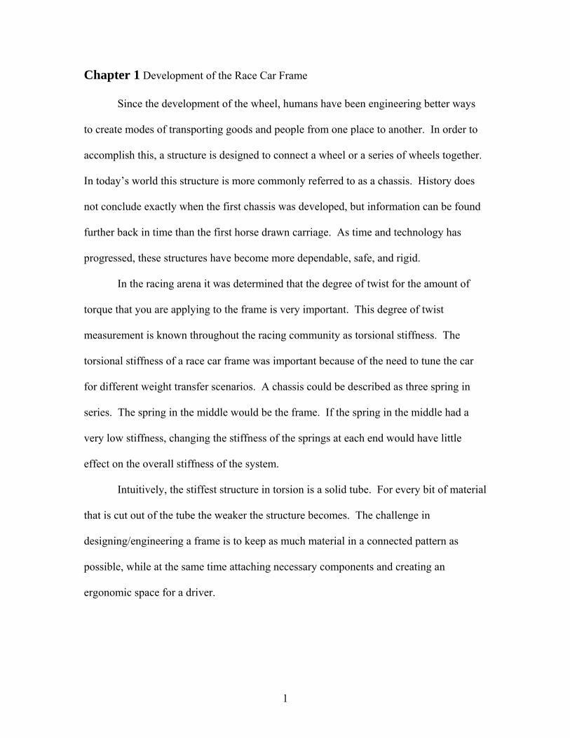
The Ladder Frame
In the world of racing, the modern chassis has been developed over the last
century and a half. The first frames in the beginning of the twentieth century were
constructed using two parallel beams laterally connected. Figure 1 shows an example of
such a construction.
Figure 1: Ladder Frame Automobile [1]
As Indy car racing began, this type of structure, referred to as a ladder frame, was
popular due to its ease of manufacture and good stiffness in vertical bending. Although,
Forbes Aird perhaps said it best “The notable feature of the frame was that it generally
flexed and twisted so much, handling was limited to trying to keep the car under control,
never mind tune it for cornering.” [1] This in itself was a great example of what should
not be happening while a chassis is making laps around a race track.
3
During the early years in the development of the racecar found the design focus to
be on engine development, not on chassis development. At this time, the role that chassis
stiffness played to create a controllable racecar was unclear. In the following years, this
role would be realized, leading to further development of the chassis. The ladder frame
in its infancy was a good start. Designers and engineers had the ability to easily
reconfigure different systems using this design. The simplicity of the design made it
extremely desirable. In fact, today the ladder frame is still implemented in most truck
and sport utility vehicle designs. Remnants can also be seen in the front structure of
modern stock cars.
The Space Frame
As conclusions were drawn about stiffness in torsion, engineers turned to space
frame construction in the 1950s and 1960s. Breakthroughs in stiffening the ladder frame
design were small and typically undesirable. Designers came to realize that adding a
second set of axially mounted beams connected with smaller tubing in a truss like
structure greatly increased the magnitude of torsional stiffness. As iterations of space
frames progressed, designers were able to orient tubes in the frame in order to better
handle and distribute the applied forces from the suspension. Initially there were not
huge leaps in frame stiffness; however with some persistence and use of triangulation,
designers were able to create a much more rigid frame. Connecting tube to tube in this
fashion allowed forces to act only along the axis of the tube, putting the tube only in
compression or tension. [1] A member loaded in this orientation only required a small
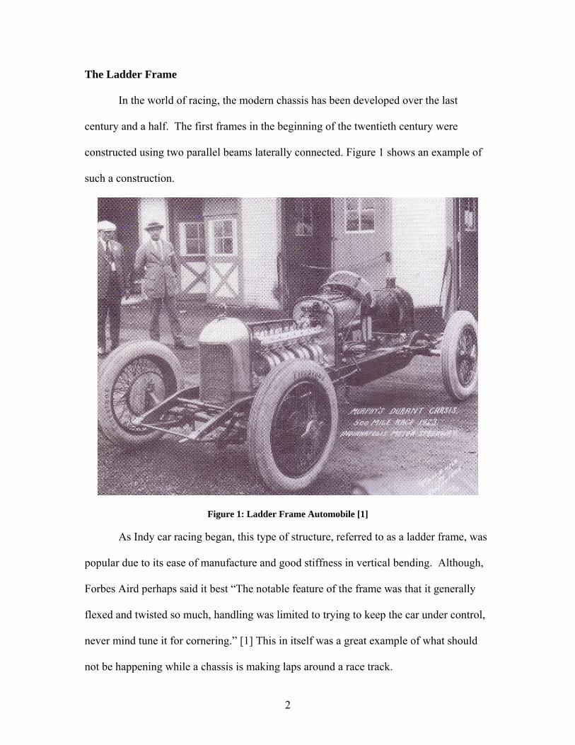
amount of material on its cross section to withstand the load. Figure 2 depicts an
example of a space frame that was developed in this era.
4
Figure 2: Space Frame Automobile [1]
With the advent of the space frame, the racecar finally evolved. Racecars became
lighter, faster and more predictable. Nevertheless, the space frame design has drawbacks.
They are complex to build and elaborate fixturing has to be created to hold points relative
to each other, prior to welding. Joints in the design(s) can be difficult to weld, which can
lead to manufacturing challenges. Despite these issues, the space frame was a major
improvement over the ladder frame.
The Composite Monocoque
A new technology was discovered in the aircraft industry that would lead to the
next evolution in frame design. The combination of stressed skin structures developed in
the depression and fibrous materials in the late 1960s, resulted in the birth of the
composite monocoque. [1] This technology revolutionized Formula One and Indy car
racing. Designers now had the ability to create a structure that was multi-purpose. The
monocoque served as the car’s structure and body, as well as provided aerodynamic flow
5
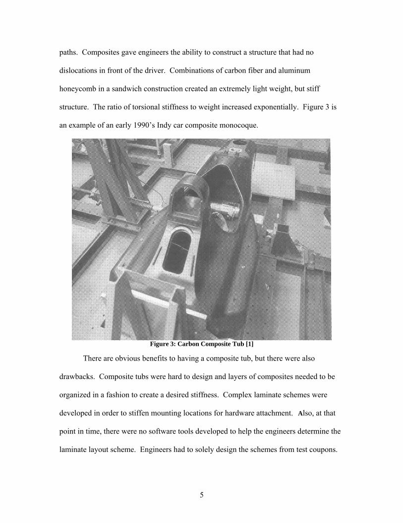
paths. Composites gave engineers the ability to construct a structure that had no
dislocations in front of the driver. Combinations of carbon fiber and aluminum
honeycomb in a sandwich construction created an extremely light weight, but stiff
structure. The ratio of torsional stiffness to weight increased exponentially. Figure 3 is
an example of an early 1990’s Indy car composite monocoque.
Figure 3: Carbon Composite Tub [1]
There are obvious benefits to having a composite tub, but there were also
drawbacks. Composite tubs were hard to design and layers of composites needed to be
organized in a fashion to create a desired stiffness. Complex laminate schemes were
developed in order to stiffen mounting locations for hardware attachment. Also, at that
point in time, there were no software tools developed to help the engineers determine the
laminate layout scheme. Engineers had to solely design the schemes from test coupons.
6
The following chapters had three major objectives. The first was to develop a
procedure for designing and validating a space frame for future teams to follow. To this
end, Chapter 2 describes how this process was previously performed and a new
recommended process. The second objective was to develop software tools that would
help speed the frame design and automate the process. The final objective was to
develop an accurate experimental test to obtain chassis stiffness on FSAE vehicles. The
text also had two less important objectives. Chapters 3 & 4 describe/document how the
frame and chassis Finite Element models are constructed for future teams to follow. The
second was to explore optimization methods for future teams to pursue.
7
Chapter 2 Background
The University of Cincinnati (UC) Formula Society of Automotive Engineers
(SAE) team has built and designed a new open-wheel chassis every year since 1993.
Traditionally, the design stage of each one of these structures was limited to three (3)
months. Throughout the infancy of the program, few analysis tools were available, so
students relied on their intuition to determine what would and would not create a rigid
chassis. Team members only utilized computers to visualize and check the clearances of
their design concepts.
Historically, UC Formula SAE vehicles have been constructed utilizing a space
frame design. Constructed from 1020 drawn over mandrel (DOM) mild steel, chassis
tubes were joined using the gas tungsten arc welding process (GTAW). The team
utilized this process because of the availability of steel, the ease of manufacturing, and
various aspects of the FSAE rules. Composite tubs would be the first choice if the
facility to produce the structure and associated expertise was available.
Frames were designed with a minimum amount of analytical and experimental
validation, prior to 2004. Typically, chassis and frame stiffness was greatly overlooked.
The time it took to understand how the frame and chassis performed was outweighed by
the time it took to actually build a car that could operate in the annual competition.
Through many of these years the UC FSAE chassis did not progress, but instead was an
annual reinvention. These structures were built with one-inch tubing, which in the end
were highly under-designed and significantly heavier than necessary.
In 2004, an analytical tool was fully introduced into the design process to help
understand how frame designs performed. ANSYS® Academic Research [11], a
8
computer based finite element analysis program was utilized in very new ways that were
not previously undertaken by the Formula SAE team. Several manual iterations with a
beam element model were performed to understand how the orientation of frame
members affected torsional stiffness as well as providing an estimate of overall weight.
With this tool also came the ability to validate the software model by correlating to
experimental modal (vibration) analysis test data. The need for a static torsion test of the
actual chassis was thought to be unnecessary at this point since the focus was on
improving torsional stiffness and reducing weight. Correlating to modal analysis data
was a reasonable and acceptable way to conclude that the FEA model was accurate. This
design process was adopted and has been implemented into each frame since 2004.
Beginning in 2005, the design process became more complicated when multiple
frame concepts were simultaneously evaluated. These design iterations were conducted
manually and an on going spreadsheet was used to document their progression and guide
the decision making process. An example of this spreadsheet can be seen in Figure 4. In
each case the ultimate goal was to drive the designs’ natural frequencies as high as
possible without adding significant amounts of mass, thus increasing the efficiency of the
frame. Once manual iterations concluded, a static solution was run to obtain a torsional
stiffness value. This process took many hours of tedious work. Attempting to understand
a single frame design was difficult enough, thus concurrently handling multiple designs
became excessively challenging. In addition, the bookkeeping was not adequately
identifying a single solution to pursue. Time eventually expired on the design process, as
a final product had to be built. As might be expected, cars were fabricated without great
confidence that the design chosen was the best it could be.

9
Figure 4: Frame Design Iteration Spreadsheet
The frame design process at the University of Cincinnati did not advance again
until 2007 when the notion of automating the design process through computer
simulation was thought to be possible. In addition, the desire existed to create a physical
test to measure the torsional stiffness of an assembled chassis. A breakthrough in
automation was made in early October 2007 when the results of ANSYS Parametric
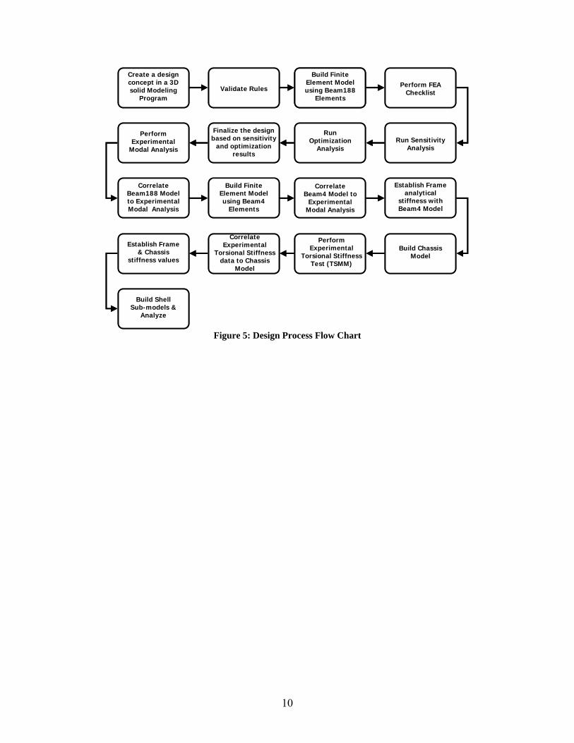
Design Language (APDL) scripting proved to be promising. Outlined in Figure 5 was
the outcome of the 2007 design process and is the recommended way for future teams to
design and validate a Formula SAE chassis. The results of these works are described in
detail in the following chapters.
10
Create a design concept in a 3D solid Modeling
ProgramValidate Rules
Build Finite Element Model using Beam188
Elements
Perform FEA Checklist
Run Sensitivity Analysis
Run Optimization
Analysis
Finalize the design based on sensitivity
and optimization results
Perform Experimental
Modal Analysis
Correlate Beam188 Model to Experimental Modal Analysis
Build Finite Element Model using Beam4
Elements
Correlate Beam4 Model to
Experimental Modal Analysis
Establish Frame analytical
stiffness with Beam4 Model
Build Chassis Model
Perform Experimental
Torsional Stiffness Test (TSMM)
Correlate Experimental
Torsional Stiffness data to Chassis
Model
Establish Frame & Chassis
stiffness values
Build Shell Sub-models &
Analyze
Create a design concept in a 3D solid Modeling
ProgramValidate Rules
Build Finite Element Model using Beam188
Elements
Build Finite Element Model using Beam188
Elements
Perform FEA Checklist
Run Sensitivity Analysis
Run Optimization
Analysis
Finalize the design based on sensitivity
and optimization results
Perform Experimental
Modal Analysis
Correlate Beam188 Model to Experimental Modal Analysis
Build Finite Element Model using Beam4
Elements
Correlate Beam4 Model to
Experimental Modal Analysis
Establish Frame analytical
stiffness with Beam4 Model
Build Chassis Model
Perform Experimental
Torsional Stiffness Test (TSMM)
Correlate Experimental
Torsional Stiffness data to Chassis
Model
Establish Frame & Chassis
stiffness values
Build Shell Sub-models &
Analyze
Figure 5: Design Process Flow Chart
11
Chapter 3 Frame Model
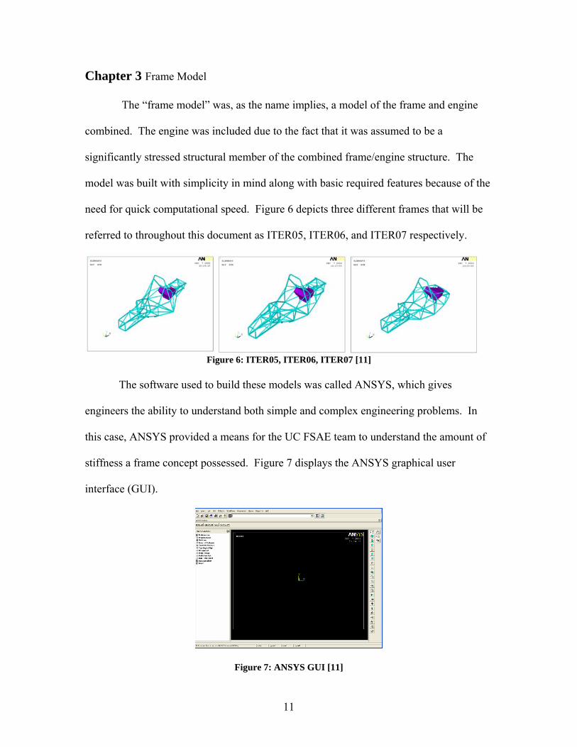
The “frame model” was, as the name implies, a model of the frame and engine
combined. The engine was included due to the fact that it was assumed to be a
significantly stressed structural member of the combined frame/engine structure. The
model was built with simplicity in mind along with basic required features because of the
need for quick computational speed. Figure 6 depicts three different frames that will be
referred to throughout this document as ITER05, ITER06, and ITER07 respectively.
Figure 6: ITER05, ITER06, ITER07 [11]
The software used to build these models was called ANSYS, which gives
engineers the ability to understand both simple and complex engineering problems. In
this case, ANSYS provided a means for the UC FSAE team to understand the amount of
stiffness a frame concept possessed. Figure 7 displays the ANSYS graphical user
interface (GUI).
Figure 7: ANSYS GUI [11]
12
Geometry Construction
The UC FSAE team’s model began its creation in another program called Solid
Edge [15], a three dimensional solid modeling program. Before any analysis work
commenced, all tubes were modeled as an assembly to ensure proper orientation and
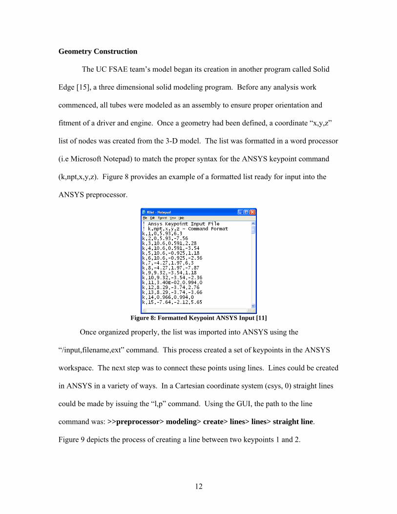
fitment of a driver and engine. Once a geometry had been defined, a coordinate “x,y,z”
list of nodes was created from the 3-D model. The list was formatted in a word processor
(i.e Microsoft Notepad) to match the proper syntax for the ANSYS keypoint command
(k,npt,x,y,z). Figure 8 provides an example of a formatted list ready for input into the
ANSYS preprocessor.
Figure 8: Formatted Keypoint ANSYS Input [11]
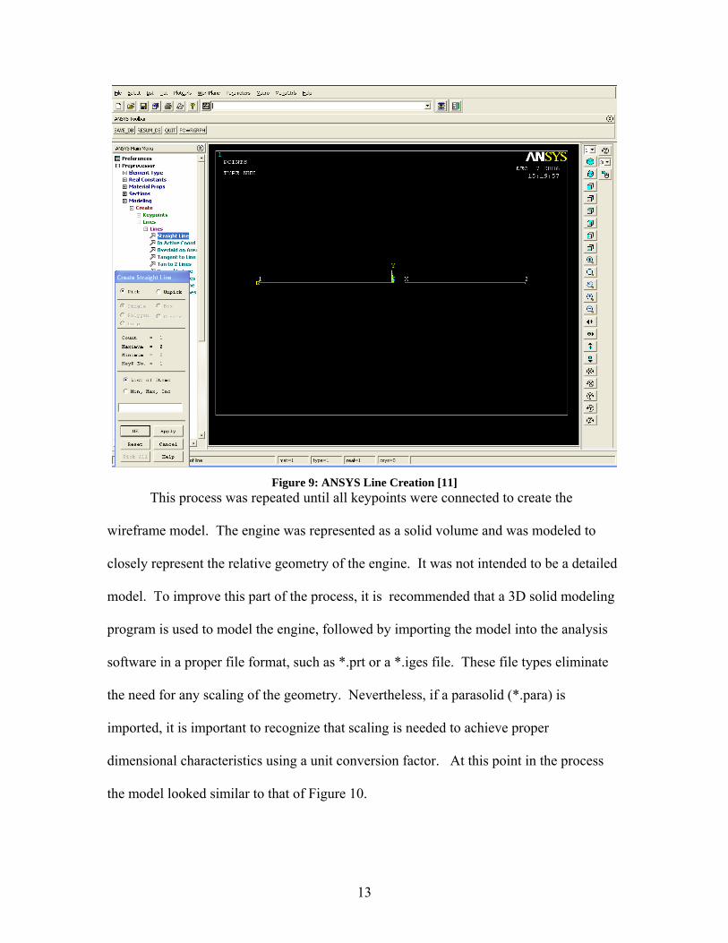
Once organized properly, the list was imported into ANSYS using the
“/input,filename,ext” command. This process created a set of keypoints in the ANSYS
workspace. The next step was to connect these points using lines. Lines could be created
in ANSYS in a variety of ways. In a Cartesian coordinate system (csys, 0) straight lines
could be made by issuing the “l,p” command. Using the GUI, the path to the line
command was: >>preprocessor> modeling> create> lines> lines> straight line.
Figure 9 depicts the process of creating a line between two keypoints 1 and 2.
13
Figure 9: ANSYS Line Creation [11]
This process was repeated until all keypoints were connected to create the
wireframe model. The engine was represented as a solid volume and was modeled to
closely represent the relative geometry of the engine. It was not intended to be a detailed
model. To improve this part of the process, it is recommended that a 3D solid modeling
program is used to model the engine, followed by importing the model into the analysis
software in a proper file format, such as *.prt or a *.iges file. These file types eliminate
the need for any scaling of the geometry. Nevertheless, if a parasolid (*.para) is
imported, it is important to recognize that scaling is needed to achieve proper
dimensional characteristics using a unit conversion factor. At this point in the process
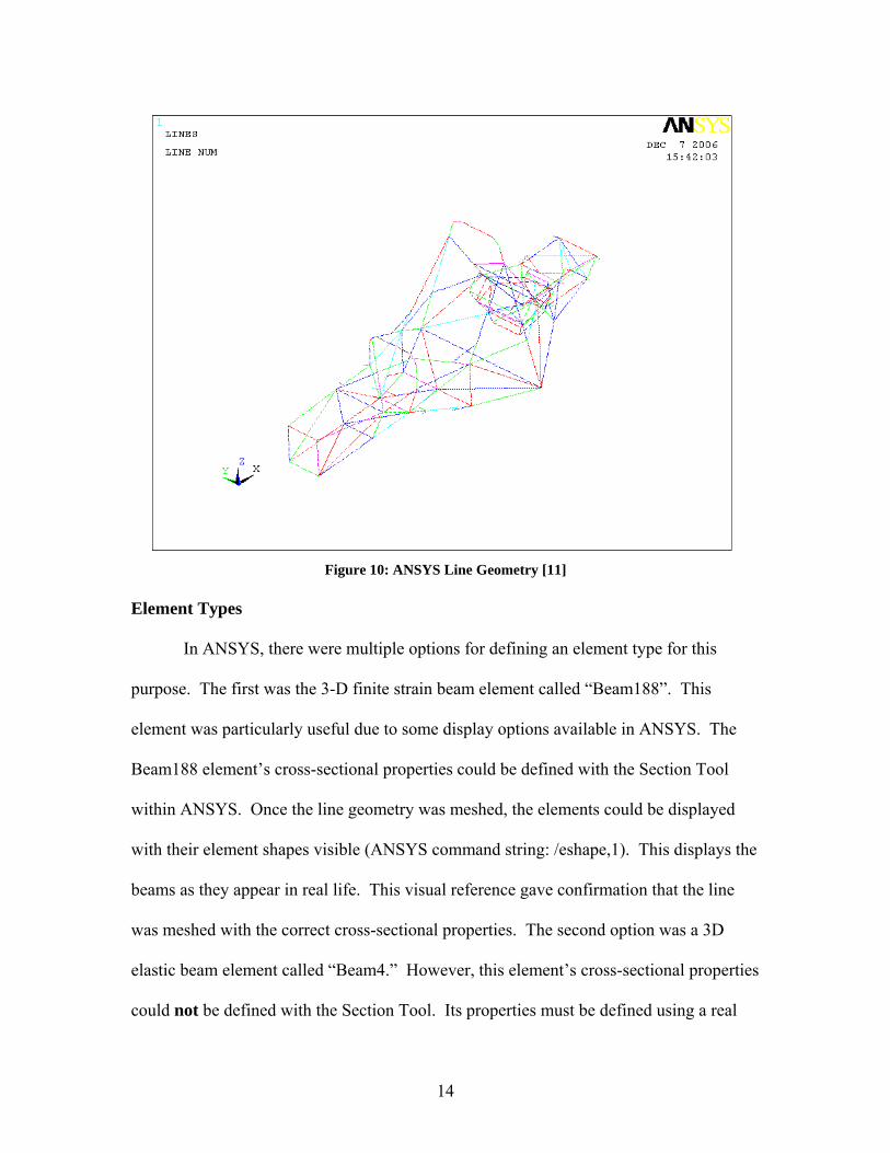
the model looked similar to that of Figure 10.
14
Figure 10: ANSYS Line Geometry [11]
Element Types
In ANSYS, there were multiple options for defining an element type for this
purpose. The first was the 3-D finite strain beam element called “Beam188”. This
element was particularly useful due to some display options available in ANSYS. The
Beam188 element’s cross-sectional properties could be defined with the Section Tool
within ANSYS. Once the line geometry was meshed, the elements could be displayed
with their element shapes visible (ANSYS command string: /eshape,1). This displays the
beams as they appear in real life. This visual reference gave confirmation that the line
was meshed with the correct cross-sectional properties. The second option was a 3D
elastic beam element called “Beam4.” However, this element’s cross-sectional properties
could not be defined with the Section Tool. Its properties must be defined using a real
15
constant [13]. Nevertheless, with either option there were distinct advantages, as well as
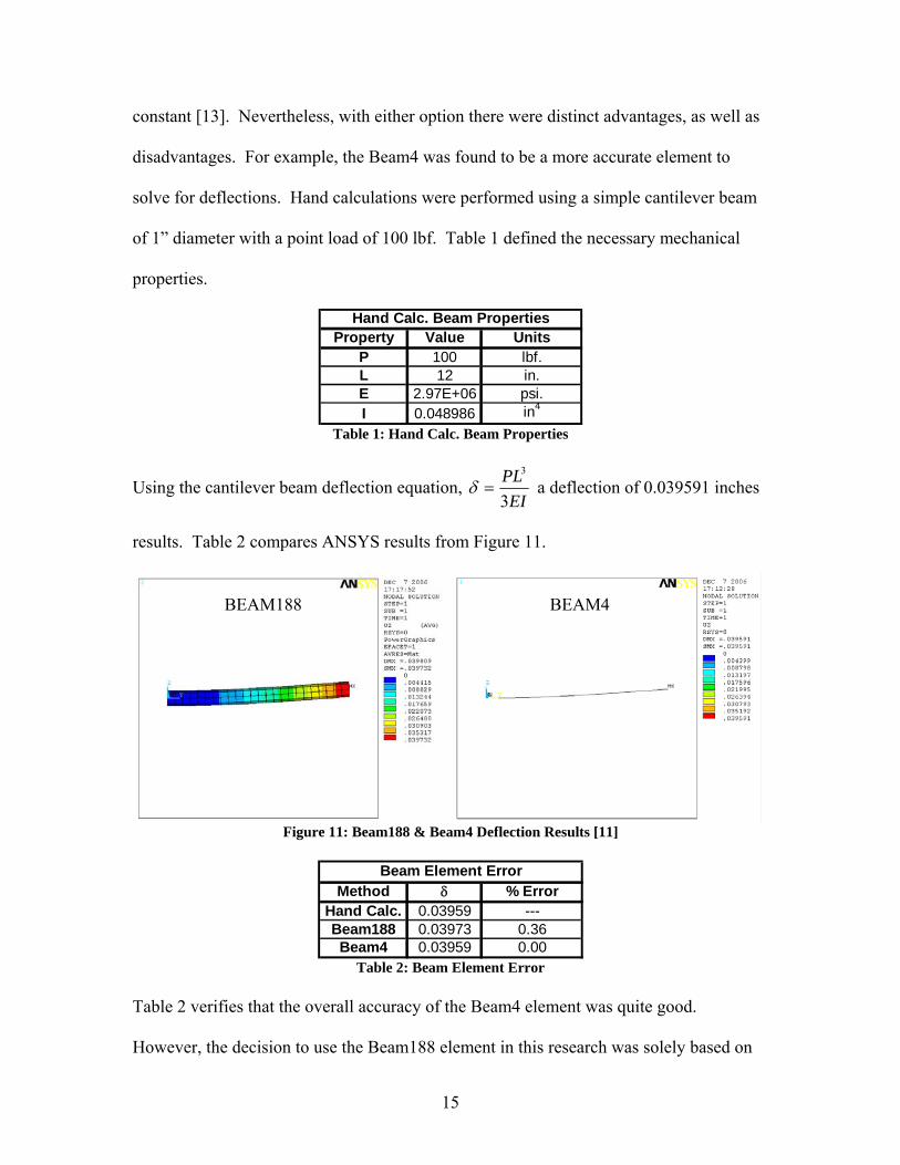
disadvantages. For example, the Beam4 was found to be a more accurate element to
solve for deflections. Hand calculations were performed using a simple cantilever beam
of 1” diameter with a point load of 100 lbf. Table 1 defined the necessary mechanical
properties.
Hand Calc. Beam PropertiesProperty Value Units
P 100 lbf.L 12 in.E 2.97E+06 psi.I 0.048986 in4
Table 1: Hand Calc. Beam Properties
Using the cantilever beam deflection equation, EI
PL3
3
=δ a deflection of 0.039591 inches
results. Table 2 compares ANSYS results from Figure 11.
Figure 11: Beam188 & Beam4 Deflection Results [11]
Beam Element Error
Method δ % ErrorHand Calc. 0.03959 ---Beam188 0.03973 0.36Beam4 0.03959 0.00
Table 2: Beam Element Error Table 2 verifies that the overall accuracy of the Beam4 element was quite good.
However, the decision to use the Beam188 element in this research was solely based on
BEAM188 BEAM4
16
the ability to write scripts quickly, with less complexity, utilizing section properties as
opposed to real constants. For the purpose of stiffness calculations, the Beam188
element was sufficient for doing comparison and design studies. Although, it must be
noted that the Beam4 element was the correct element to use for deriving an “actual”
empirical number for frame and/or chassis stiffness.
Material & Section Properties
Material and Section properties were the next items to be defined in the model.
Young’s Modulus (EX), Poisson’s Ratio (PRXY), and density had to be defined at a
minimum. Material properties were quite simple to define, yet were the most overlooked
item when the model was not responding properly. In particular, it was important to
make some assumptions as to how the gravity field was defined. Since this research
involved a racecar operating in a 1-G field, it was necessary to define that in the model.
Gravity could be defined in two ways. The first and recommended way was to scale the
density down by 1-G. Another way was to define an inertial gravity field using the
“accel” command in ANSYS. If the gravity field is not defined, natural frequencies
cannot be accurately measured for a simulation in a 1-G field. Temperature effects were
not considered because testing for torsional stiffness was a static measurement done with
the engine off in a controlled environment, indoors. Therefore, it was not necessary to
define a temperature dependant material property table in ANSYS.
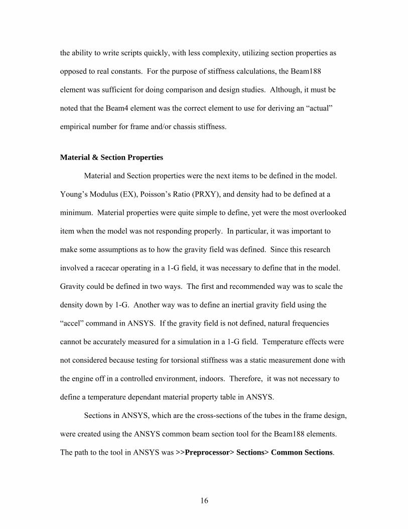
Sections in ANSYS, which are the cross-sections of the tubes in the frame design,
were created using the ANSYS common beam section tool for the Beam188 elements.
The path to the tool in ANSYS was >>Preprocessor> Sections> Common Sections.
17
Figure 12 was a display of this tool. This tool was easily implemented when using
Beam188 elements.
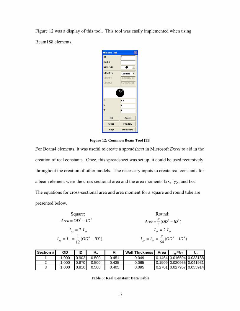
Figure 12: Common Beam Tool [11] For Beam4 elements, it was useful to create a spreadsheet in Microsoft Excel to aid in the
creation of real constants. Once, this spreadsheet was set up, it could be used recursively
throughout the creation of other models. The necessary inputs to create real constants for
a beam element were the cross sectional area and the area moments Ixx, Iyy, and Izz.
The equations for cross-sectional area and area moment for a square and round tube are
presented below.
Square: Round: 22 IDODArea −= )(
422 IDODArea −=
π
xxxx II 2= xxxx II 2=
)(121 44 IDODII zzyy −== )(
6444 IDODII zzyy −==
π
Section # OD ID Ro Ri Wall Thickness Area Iyy=IZZ Ixx
1 1.000 0.902 0.500 0.451 0.049 0.1464 0.016594 0.0331882 1.000 0.870 0.500 0.435 0.065 0.1909 0.020965 0.0419313 1.000 0.810 0.500 0.405 0.095 0.2701 0.027957 0.055914
Table 3: Real Constant Data Table
18
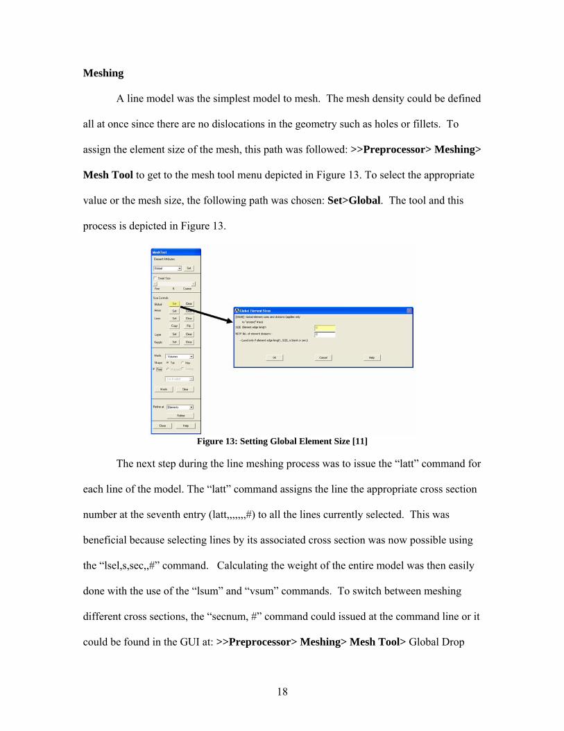
Meshing
A line model was the simplest model to mesh. The mesh density could be defined
all at once since there are no dislocations in the geometry such as holes or fillets. To
assign the element size of the mesh, this path was followed: >>Preprocessor> Meshing>
Mesh Tool to get to the mesh tool menu depicted in Figure 13. To select the appropriate
value or the mesh size, the following path was chosen: Set>Global. The tool and this
process is depicted in Figure 13.
Figure 13: Setting Global Element Size [11]
The next step during the line meshing process was to issue the “latt” command for
each line of the model. The “latt” command assigns the line the appropriate cross section
number at the seventh entry (latt,,,,,,,#) to all the lines currently selected. This was
beneficial because selecting lines by its associated cross section was now possible using
the “lsel,s,sec,,#” command. Calculating the weight of the entire model was then easily
done with the use of the “lsum” and “vsum” commands. To switch between meshing
different cross sections, the “secnum, #” command could issued at the command line or it
could be found in the GUI at: >>Preprocessor> Meshing> Mesh Tool> Global Drop
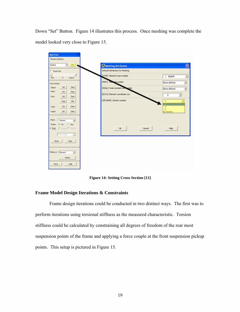
19
Down “Set” Button. Figure 14 illustrates this process. Once meshing was complete the
model looked very close to Figure 15.
Figure 14: Setting Cross Section [11]
Frame Model Design Iterations & Constraints
Frame design iterations could be conducted in two distinct ways. The first was to
perform iterations using torsional stiffness as the measured characteristic. Torsion
stiffness could be calculated by constraining all degrees of freedom of the rear most
suspension points of the frame and applying a force couple at the front suspension pickup
points. This setup is pictured in Figure 15.
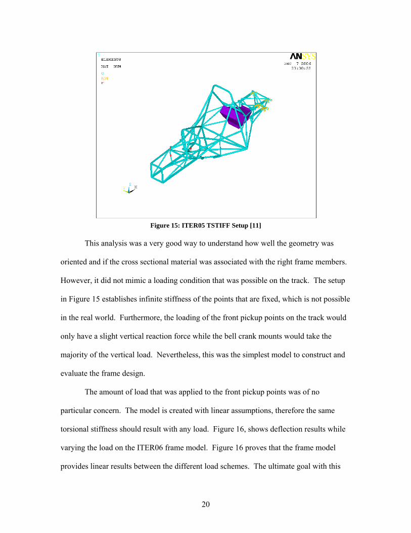
20
Figure 15: ITER05 TSTIFF Setup [11]
This analysis was a very good way to understand how well the geometry was
oriented and if the cross sectional material was associated with the right frame members.
However, it did not mimic a loading condition that was possible on the track. The setup
in Figure 15 establishes infinite stiffness of the points that are fixed, which is not possible
in the real world. Furthermore, the loading of the front pickup points on the track would
only have a slight vertical reaction force while the bell crank mounts would take the
majority of the vertical load. Nevertheless, this was the simplest model to construct and
evaluate the frame design.
The amount of load that was applied to the front pickup points was of no
particular concern. The model is created with linear assumptions, therefore the same
torsional stiffness should result with any load. Figure 16, shows deflection results while
varying the load on the ITER06 frame model. Figure 16 proves that the frame model
provides linear results between the different load schemes. The ultimate goal with this
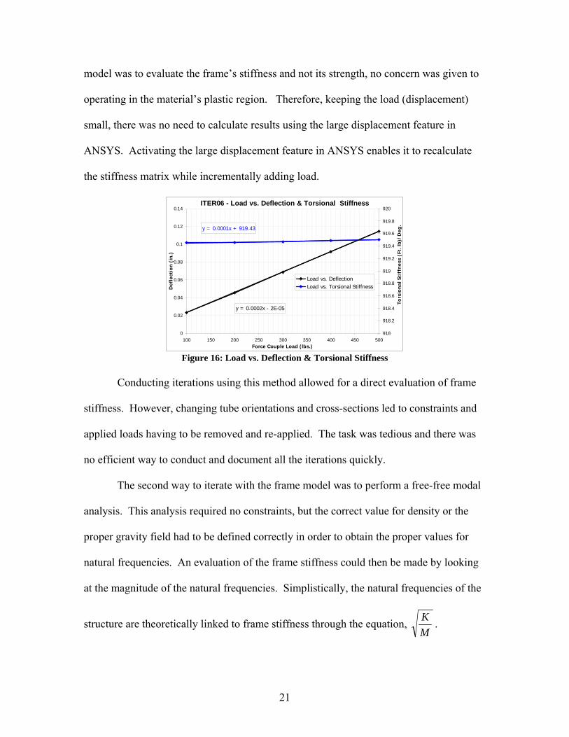
21
model was to evaluate the frame’s stiffness and not its strength, no concern was given to
operating in the material’s plastic region. Therefore, keeping the load (displacement)
small, there was no need to calculate results using the large displacement feature in
ANSYS. Activating the large displacement feature in ANSYS enables it to recalculate
the stiffness matrix while incrementally adding load.
ITER06 - Load vs. Deflection & Torsional Stiffness
y = 0.0001x + 919.43
y = 0.0002x - 2E-05
0
0.02
0.04
0.06
0.08
0.1
0.12
0.14
100 150 200 250 300 350 400 450 500Force Couple Load (lbs.)
Def
lect
ion
(in
.)
918
918.2
918.4
918.6
918.8
919
919.2
919.4
919.6
919.8
920
Tors
ion
al S
tiff
nes
s (F
t. lb
)/D
eg.
Load vs. DeflectionLoad vs. Torsional Stiffness
Figure 16: Load vs. Deflection & Torsional Stiffness
Conducting iterations using this method allowed for a direct evaluation of frame
stiffness. However, changing tube orientations and cross-sections led to constraints and
applied loads having to be removed and re-applied. The task was tedious and there was
no efficient way to conduct and document all the iterations quickly.
The second way to iterate with the frame model was to perform a free-free modal
analysis. This analysis required no constraints, but the correct value for density or the
proper gravity field had to be defined correctly in order to obtain the proper values for
natural frequencies. An evaluation of the frame stiffness could then be made by looking
at the magnitude of the natural frequencies. Simplistically, the natural frequencies of the
structure are theoretically linked to frame stiffness through the equation, MK .
22
Therefore, organizing the frame tubes and cross-sections to shift natural frequencies into
a higher frequency band, while minimizing the mass, stiffens the frame.
Running a modal analysis in ANSYS was very easy, but at times it could be
difficult to understand how the design was improving. While, conducting iterations with
modal analysis and comparing the natural frequencies from one iteration to the next it
could get confusing. It was essential to have a deep understanding as to what was
happening from one iteration to the next. When a cross section of a certain tube was
iterated, both mass and stiffness were changing. In some instances, this produced a result
where one natural frequency went up and while another natural frequency went down.
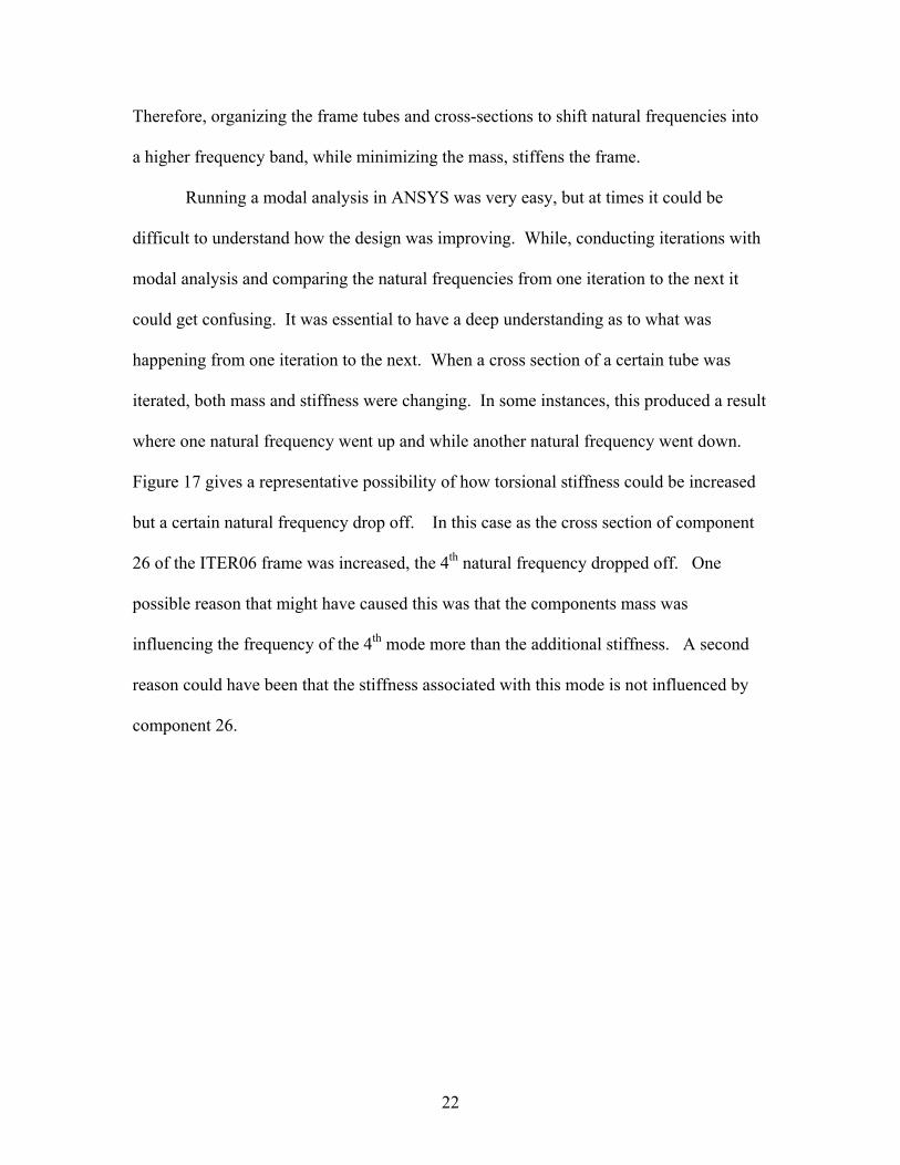
Figure 17 gives a representative possibility of how torsional stiffness could be increased
but a certain natural frequency drop off. In this case as the cross section of component
26 of the ITER06 frame was increased, the 4th natural frequency dropped off. One
possible reason that might have caused this was that the components mass was
influencing the frequency of the 4th mode more than the additional stiffness. A second
reason could have been that the stiffness associated with this mode is not influenced by
component 26.
23
ITER06 Comp. 26 Torsional Stiff. vs. 4th Natural Freq.
y = 9.0182x + 651.42
600
620
640
660
680
700
720
740
760
780
800
820
1 2 3 4 5 6 7 8 9 10 11 12 13 14 15 16Ansys Cross Section Number
Tors
ion
al S
tiff
ness
(Ft
.*lb
)/D
eg.
67
68
69
70
71
72
73
74
75
Freq
uen
cy (
Hz)
Torsional Stiffness
4th Natural Frequencies
Linear (Torsional Stiffness)
Figure 17: Torsional Stiffness vs. 4th Natural Frequencies
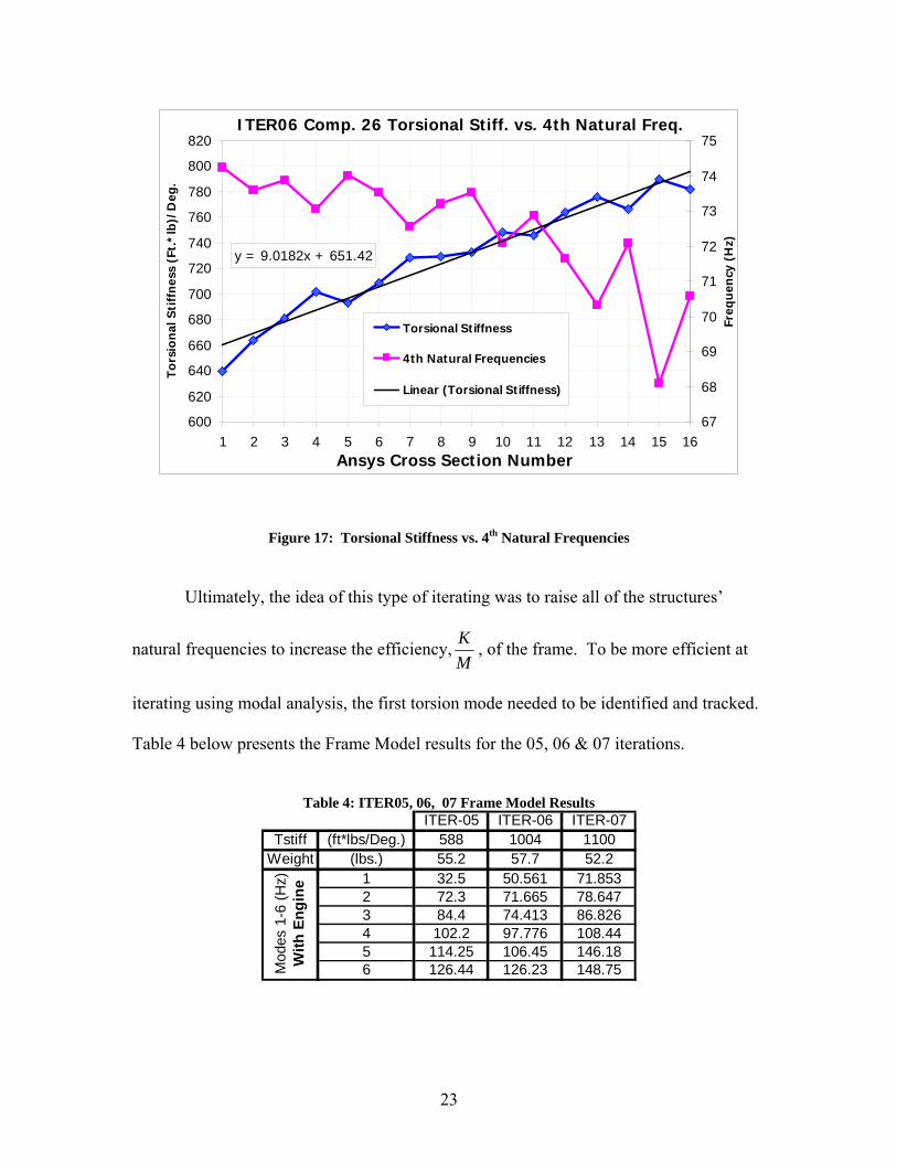
Ultimately, the idea of this type of iterating was to raise all of the structures’
natural frequencies to increase the efficiency,MK , of the frame. To be more efficient at
iterating using modal analysis, the first torsion mode needed to be identified and tracked.
Table 4 below presents the Frame Model results for the 05, 06 & 07 iterations.
Table 4: ITER05, 06, 07 Frame Model Results
ITER-05 ITER-06 ITER-07Tstiff (ft*lbs/Deg.) 588 1004 1100
Weight (lbs.) 55.2 57.7 52.21 32.5 50.561 71.8532 72.3 71.665 78.6473 84.4 74.413 86.8264 102.2 97.776 108.445 114.25 106.45 146.186 126.44 126.23 148.75M
odes
1-6
(Hz)
With
Eng
ine
24
Chapter 4 Chassis Model
Trying to model a fully operational chassis in ANSYS was not a simple task. For
this research, a sound knowledge of the ANSYS software program was essential. For
the novice ANSYS user, this particular task could be very intimidating until a good
knowledge base has been established. The following outlines the modeling techniques to
assist in making this easier.
It would be ideal at this point in the analysis effort that the frame model be
correlated to experimental modal data. If experimental modal data is not available, the
frame model should at least be run through a series of model checks to gain confidence in
the results that it will produce. Reference Appendix A for a representative checklist to
aid in this process. This checklist, in most cases, will save time and minimize frustration.
It suggests that a modal solution be run on the model to make sure that the first natural
frequency (Mode 1 or 7) should be at or above 10 Hz. If this was not the case, more than
likely there was an unconnected line at an existing keypoint. As an extra precaution, it
was good habit to plot the first six mode shapes and to ensure everything looks like a
system mode and not a local mode due to unconnected nodes. Also, prior to running a
modal solution, a 1 G static solution should be run. This check verifies that densities
have been correctly assigned and the sum of the reactions at all the constraint points
equals the predicted weight of the frame. A reaction printout in ANSYS can be obtained
by typing “prrs” at the command line while in the post processor (/post1) with the results
file loaded.
25
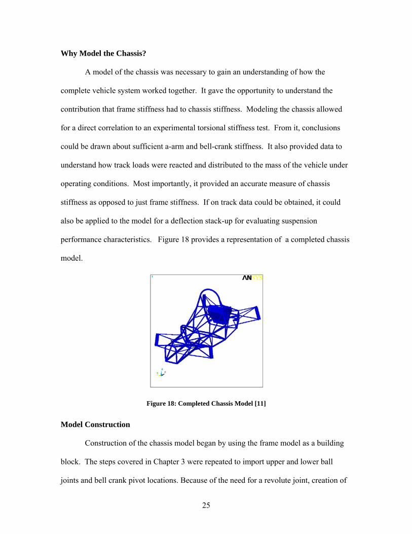
Why Model the Chassis?
A model of the chassis was necessary to gain an understanding of how the
complete vehicle system worked together. It gave the opportunity to understand the
contribution that frame stiffness had to chassis stiffness. Modeling the chassis allowed
for a direct correlation to an experimental torsional stiffness test. From it, conclusions
could be drawn about sufficient a-arm and bell-crank stiffness. It also provided data to
understand how track loads were reacted and distributed to the mass of the vehicle under
operating conditions. Most importantly, it provided an accurate measure of chassis
stiffness as opposed to just frame stiffness. If on track data could be obtained, it could
also be applied to the model for a deflection stack-up for evaluating suspension
performance characteristics. Figure 18 provides a representation of a completed chassis
model.
Figure 18: Completed Chassis Model [11]
Model Construction
Construction of the chassis model began by using the frame model as a building
block. The steps covered in Chapter 3 were repeated to import upper and lower ball
joints and bell crank pivot locations. Because of the need for a revolute joint, creation of
26
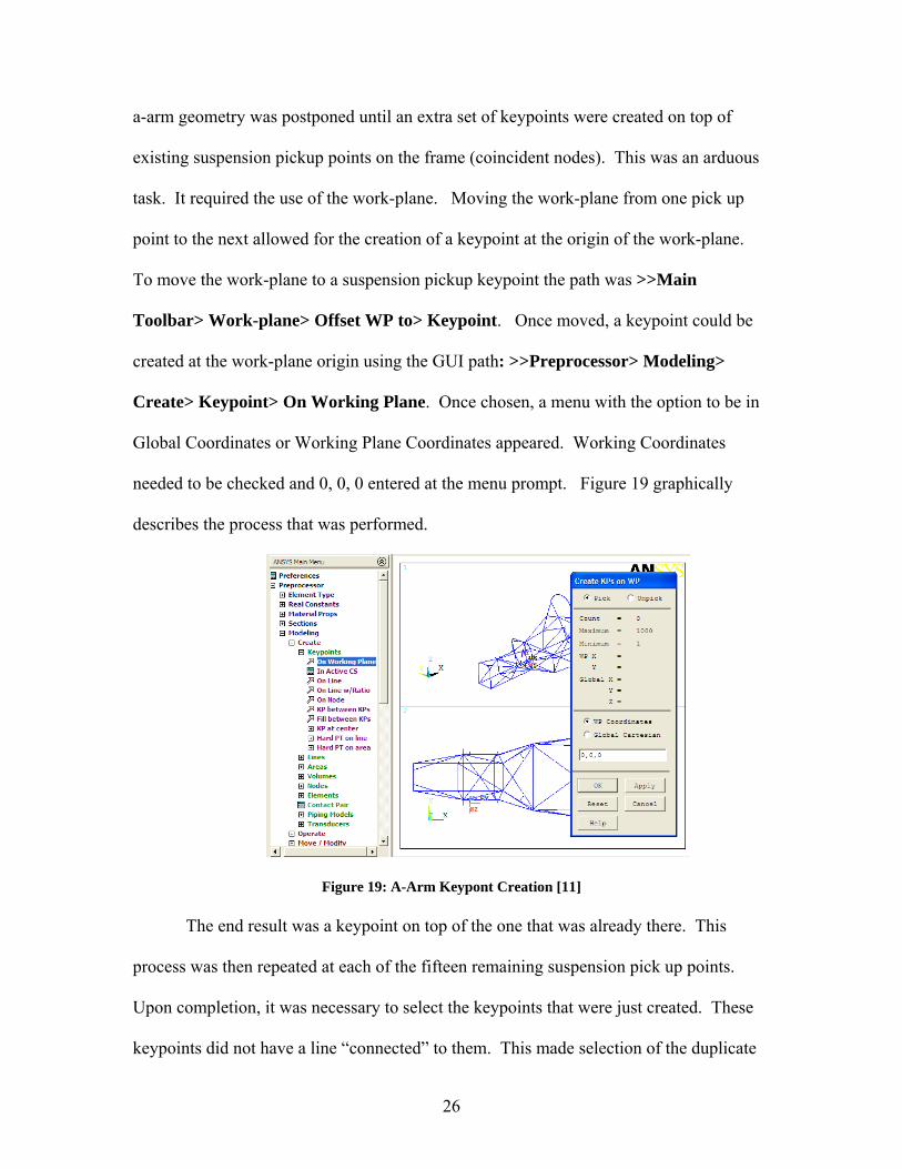
a-arm geometry was postponed until an extra set of keypoints were created on top of
existing suspension pickup points on the frame (coincident nodes). This was an arduous
task. It required the use of the work-plane. Moving the work-plane from one pick up
point to the next allowed for the creation of a keypoint at the origin of the work-plane.
To move the work-plane to a suspension pickup keypoint the path was >>Main
Toolbar> Work-plane> Offset WP to> Keypoint. Once moved, a keypoint could be
created at the work-plane origin using the GUI path: >>Preprocessor> Modeling>
Create> Keypoint> On Working Plane. Once chosen, a menu with the option to be in
Global Coordinates or Working Plane Coordinates appeared. Working Coordinates
needed to be checked and 0, 0, 0 entered at the menu prompt. Figure 19 graphically
describes the process that was performed.
Figure 19: A-Arm Keypont Creation [11]
The end result was a keypoint on top of the one that was already there. This
process was then repeated at each of the fifteen remaining suspension pick up points.
Upon completion, it was necessary to select the keypoints that were just created. These
keypoints did not have a line “connected” to them. This made selection of the duplicate
27
keypoints fairly difficult. This issue was dodged by issuing the “allselect” command,
which selected everything in the database. Next, the “allselect,below,line” was issued,
which selected only the keypoint that were associated under a line. Finally, the
“ksel,inve” command was issued and the keypoints were re-plotted. Issuing these three
commands consecutively selected the duplicate keypoints and any new keypoints not
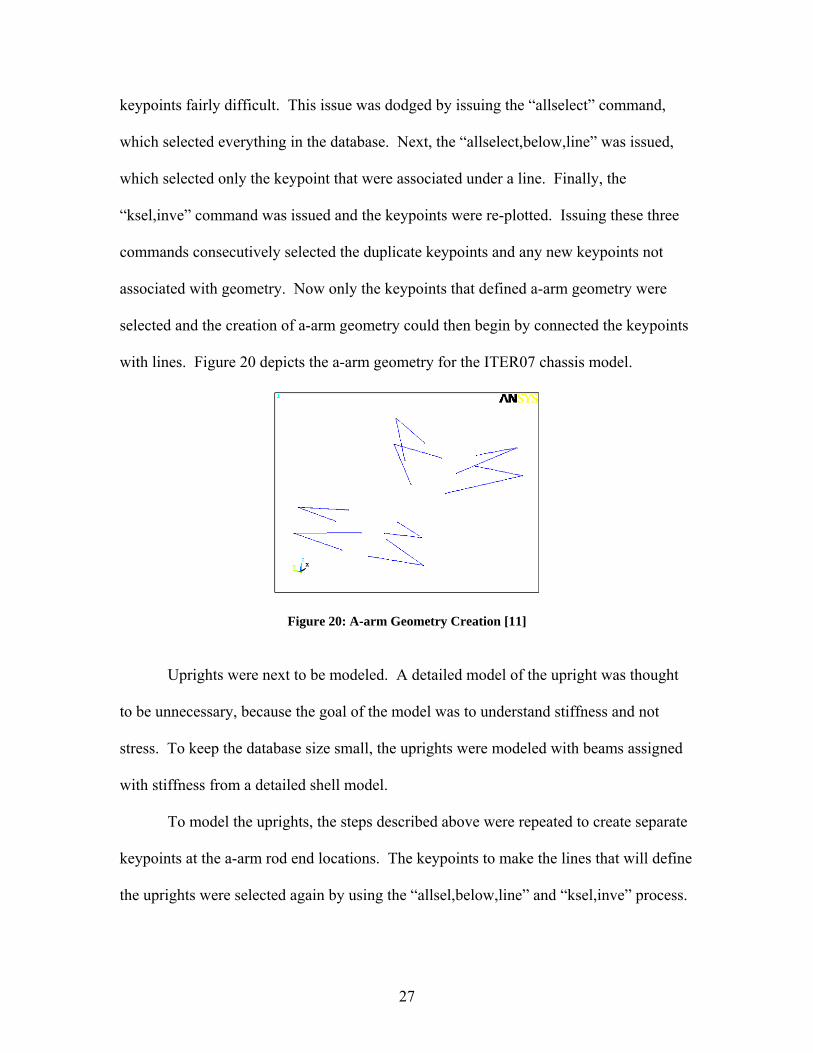
associated with geometry. Now only the keypoints that defined a-arm geometry were
selected and the creation of a-arm geometry could then begin by connected the keypoints
with lines. Figure 20 depicts the a-arm geometry for the ITER07 chassis model.
Figure 20: A-arm Geometry Creation [11]
Uprights were next to be modeled. A detailed model of the upright was thought
to be unnecessary, because the goal of the model was to understand stiffness and not
stress. To keep the database size small, the uprights were modeled with beams assigned
with stiffness from a detailed shell model.
To model the uprights, the steps described above were repeated to create separate
keypoints at the a-arm rod end locations. The keypoints to make the lines that will define
the uprights were selected again by using the “allsel,below,line” and “ksel,inve” process.
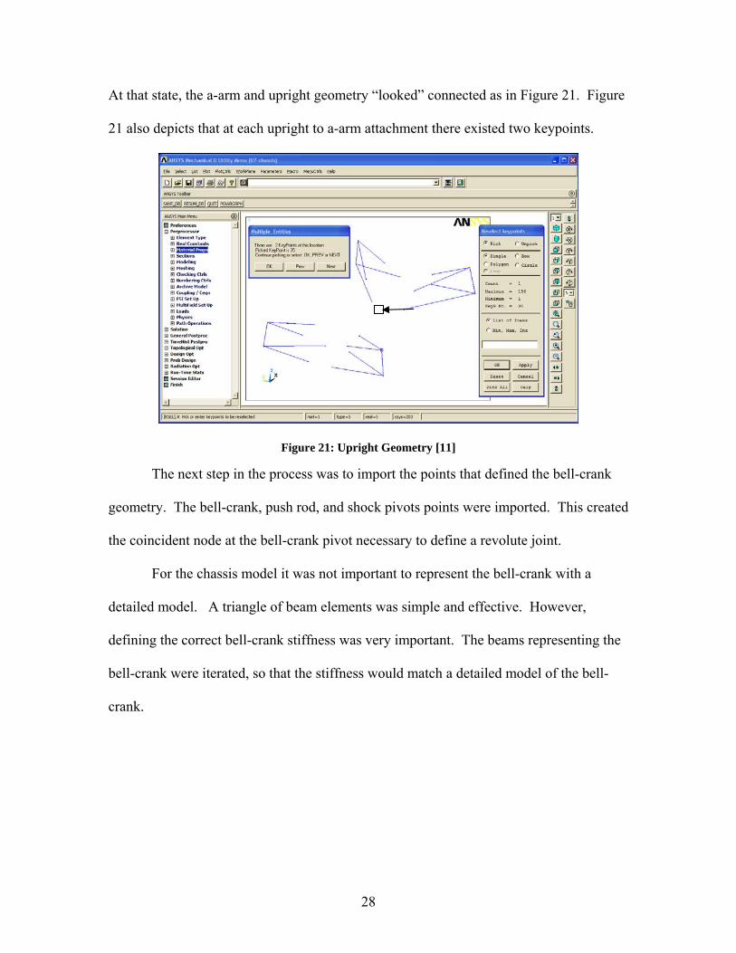
28
At that state, the a-arm and upright geometry “looked” connected as in Figure 21. Figure
21 also depicts that at each upright to a-arm attachment there existed two keypoints.
Figure 21: Upright Geometry [11]
The next step in the process was to import the points that defined the bell-crank
geometry. The bell-crank, push rod, and shock pivots points were imported. This created
the coincident node at the bell-crank pivot necessary to define a revolute joint.
For the chassis model it was not important to represent the bell-crank with a
detailed model. A triangle of beam elements was simple and effective. However,
defining the correct bell-crank stiffness was very important. The beams representing the
bell-crank were iterated, so that the stiffness would match a detailed model of the bell-
crank.
29
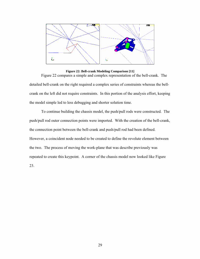
Figure 22: Bell-crank Modeling Comparison [11] Figure 22 compares a simple and complex representation of the bell-crank. The
detailed bell-crank on the right required a complex series of constraints whereas the bell-
crank on the left did not require constraints. In this portion of the analysis effort, keeping
the model simple led to less debugging and shorter solution time.
To continue building the chassis model, the push/pull rods were constructed. The
push/pull rod outer connection points were imported. With the creation of the bell-crank,
the connection point between the bell-crank and push/pull rod had been defined.
However, a coincident node needed to be created to define the revolute element between
the two. The process of moving the work-plane that was describe previously was
repeated to create this keypoint. A corner of the chassis model now looked like Figure
23.
30
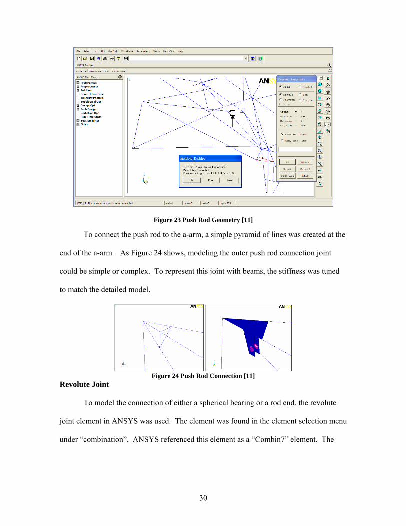
Figure 23 Push Rod Geometry [11]
To connect the push rod to the a-arm, a simple pyramid of lines was created at the
end of the a-arm . As Figure 24 shows, modeling the outer push rod connection joint
could be simple or complex. To represent this joint with beams, the stiffness was tuned
to match the detailed model.
Figure 24 Push Rod Connection [11]
Revolute Joint
To model the connection of either a spherical bearing or a rod end, the revolute
joint element in ANSYS was used. The element was found in the element selection menu
under “combination”. ANSYS referenced this element as a “Combin7” element. The
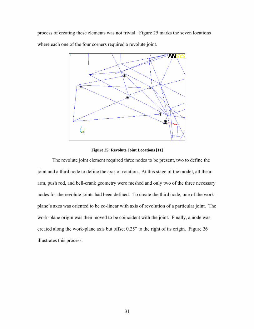
31
process of creating these elements was not trivial. Figure 25 marks the seven locations
where each one of the four corners required a revolute joint.
Figure 25: Revolute Joint Locations [11]
The revolute joint element required three nodes to be present, two to define the
joint and a third node to define the axis of rotation. At this stage of the model, all the a-
arm, push rod, and bell-crank geometry were meshed and only two of the three necessary
nodes for the revolute joints had been defined. To create the third node, one of the work-
plane’s axes was oriented to be co-linear with axis of revolution of a particular joint. The
work-plane origin was then moved to be coincident with the joint. Finally, a node was
created along the work-plane axis but offset 0.25” to the right of its origin. Figure 26
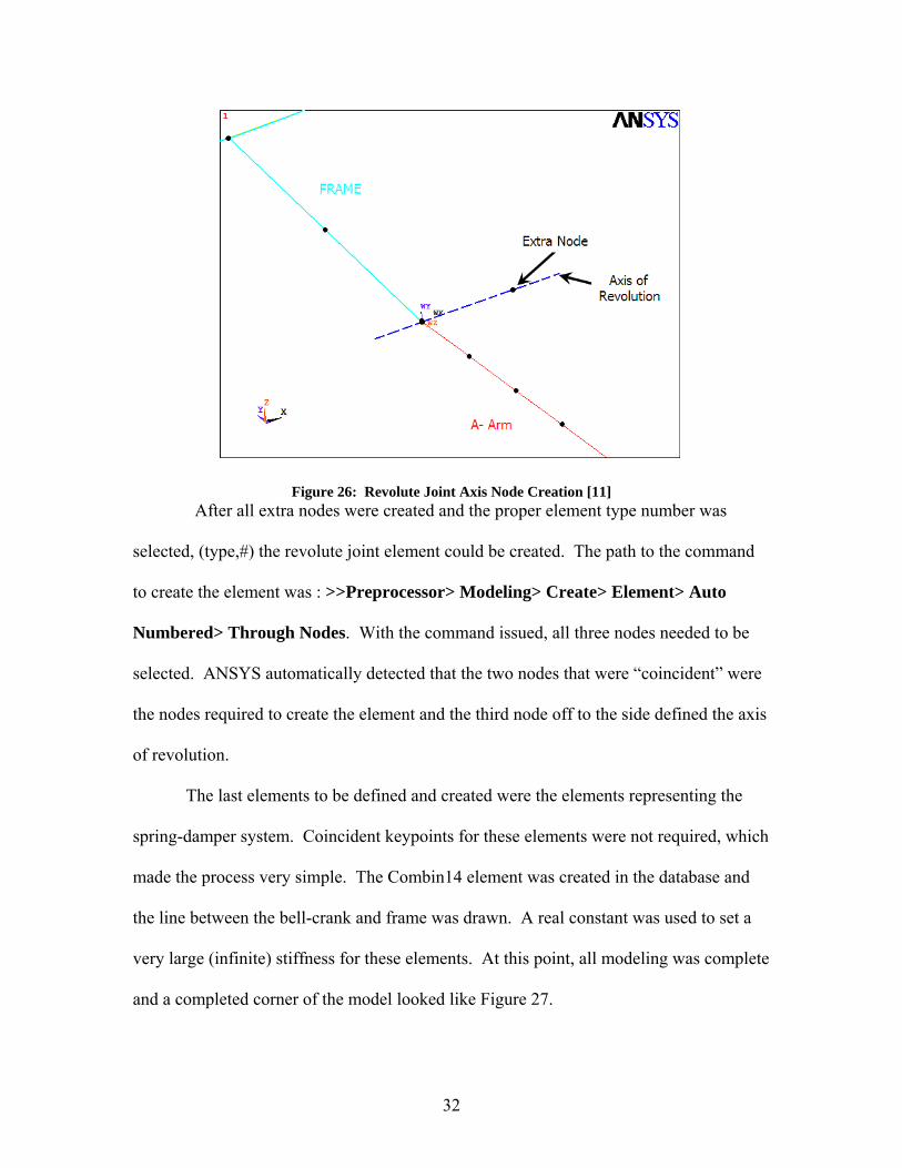
illustrates this process.
32
Figure 26: Revolute Joint Axis Node Creation [11] After all extra nodes were created and the proper element type number was
selected, (type,#) the revolute joint element could be created. The path to the command
to create the element was : >>Preprocessor> Modeling> Create> Element> Auto
Numbered> Through Nodes. With the command issued, all three nodes needed to be
selected. ANSYS automatically detected that the two nodes that were “coincident” were
the nodes required to create the element and the third node off to the side defined the axis
of revolution.
The last elements to be defined and created were the elements representing the
spring-damper system. Coincident keypoints for these elements were not required, which
made the process very simple. The Combin14 element was created in the database and
the line between the bell-crank and frame was drawn. A real constant was used to set a
very large (infinite) stiffness for these elements. At this point, all modeling was complete
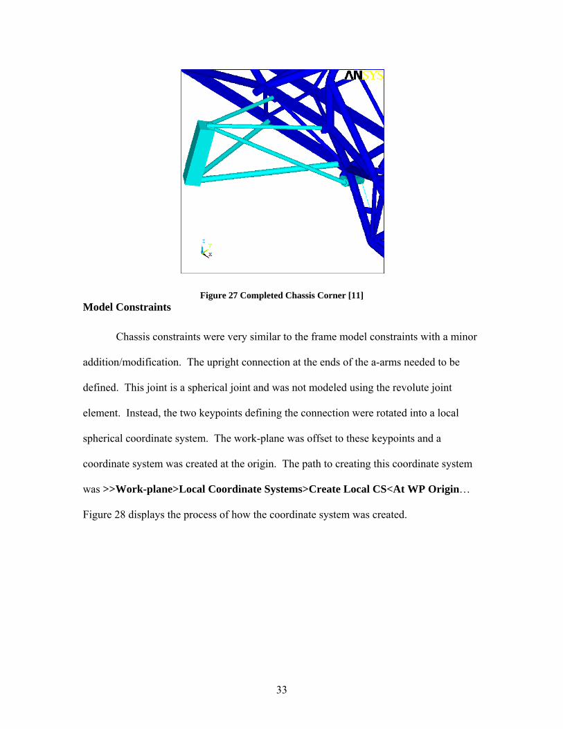
and a completed corner of the model looked like Figure 27.
33
Figure 27 Completed Chassis Corner [11] Model Constraints
Chassis constraints were very similar to the frame model constraints with a minor
addition/modification. The upright connection at the ends of the a-arms needed to be
defined. This joint is a spherical joint and was not modeled using the revolute joint
element. Instead, the two keypoints defining the connection were rotated into a local
spherical coordinate system. The work-plane was offset to these keypoints and a
coordinate system was created at the origin. The path to creating this coordinate system
was >>Work-plane>Local Coordinate Systems>Create Local CS<At WP Origin…
Figure 28 displays the process of how the coordinate system was created.
34
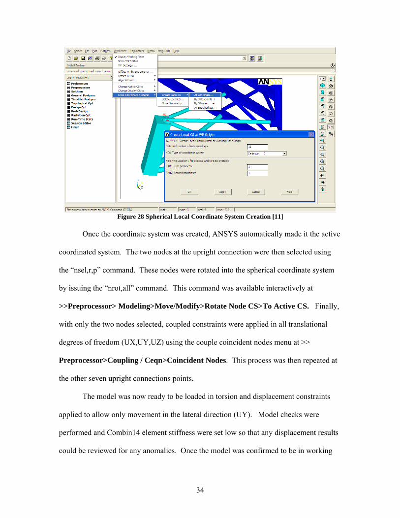
Figure 28 Spherical Local Coordinate System Creation [11]
Once the coordinate system was created, ANSYS automatically made it the active
coordinated system. The two nodes at the upright connection were then selected using
the “nsel,r,p” command. These nodes were rotated into the spherical coordinate system
by issuing the “nrot,all” command. This command was available interactively at
>>Preprocessor> Modeling>Move/Modify>Rotate Node CS>To Active CS. Finally,
with only the two nodes selected, coupled constraints were applied in all translational
degrees of freedom (UX,UY,UZ) using the couple coincident nodes menu at >>
Preprocessor>Coupling / Ceqn>Coincident Nodes. This process was then repeated at
the other seven upright connections points.
The model was now ready to be loaded in torsion and displacement constraints
applied to allow only movement in the lateral direction (UY). Model checks were
performed and Combin14 element stiffness were set low so that any displacement results
could be reviewed for any anomalies. Once the model was confirmed to be in working
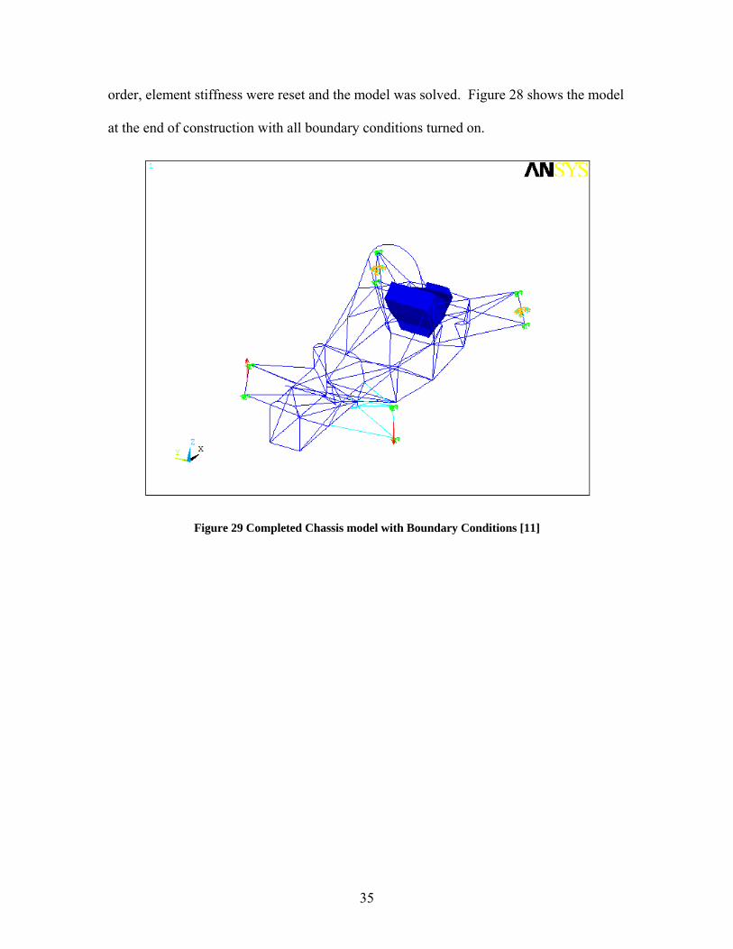
35
order, element stiffness were reset and the model was solved. Figure 28 shows the model
at the end of construction with all boundary conditions turned on.
Figure 29 Completed Chassis model with Boundary Conditions [11]
36
Chapter 5 Sensitivity Analysis & Optimization Tools
Sensitivity Analysis
Once geometry had been defined for a frame design, the next task was to
determine what size cross section was appropriate for each member in the geometry.
This was not a very intuitive process when manually iterating. It was extremely difficult
to get an overall picture as to what tube was more important to stiffness as opposed to
another. An automated method was conceived to rank frame members in order of their
sensitivity to torsional stiffness, to aid in alleviating this issue.
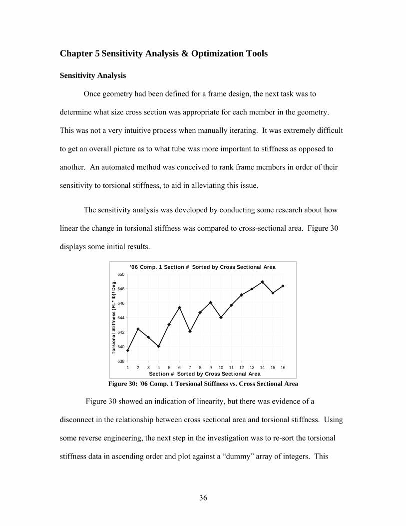
The sensitivity analysis was developed by conducting some research about how
linear the change in torsional stiffness was compared to cross-sectional area. Figure 30
displays some initial results.
'06 Comp. 1 Section # Sorted by Cross Sectional Area
638
640
642
644
646
648
650
1 2 3 4 5 6 7 8 9 10 11 12 13 14 15 16Section # Sorted by Cross Sectional Area
Tors
iona
l Sti
ffne
ss (
Ft.*
lb)/
Deg
.
Figure 30: '06 Comp. 1 Torsional Stiffness vs. Cross Sectional Area
Figure 30 showed an indication of linearity, but there was evidence of a
disconnect in the relationship between cross sectional area and torsional stiffness. Using
some reverse engineering, the next step in the investigation was to re-sort the torsional
stiffness data in ascending order and plot against a “dummy” array of integers. This
37
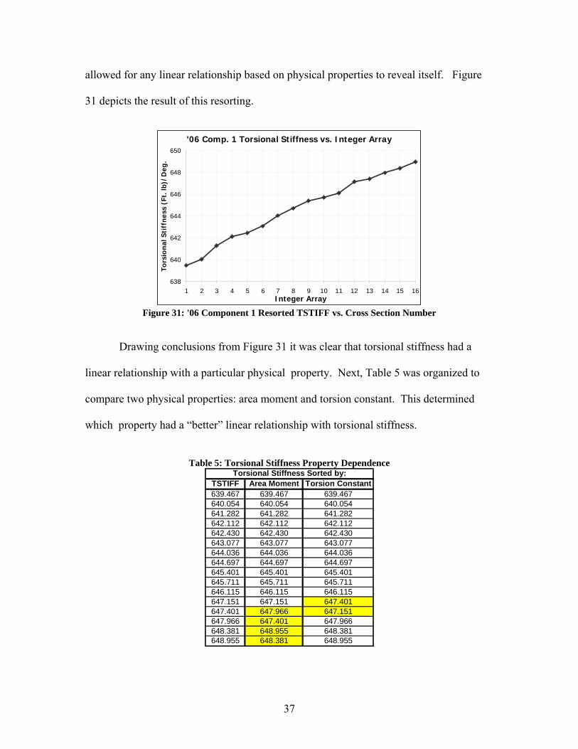
allowed for any linear relationship based on physical properties to reveal itself. Figure
31 depicts the result of this resorting.
'06 Comp. 1 Torsional Stiffness vs. Integer Array
638
640
642
644
646
648
650
1 2 3 4 5 6 7 8 9 10 11 12 13 14 15 16Integer Array
Tors
ion
al S
tiff
nes
s (F
t. lb
)/D
eg.
Figure 31: '06 Component 1 Resorted TSTIFF vs. Cross Section Number
Drawing conclusions from Figure 31 it was clear that torsional stiffness had a
linear relationship with a particular physical property. Next, Table 5 was organized to
compare two physical properties: area moment and torsion constant. This determined
which property had a “better” linear relationship with torsional stiffness.
Table 5: Torsional Stiffness Property Dependence
Torsional Stiffness Sorted by:TSTIFF Area Moment Torsion Constant639.467 639.467 639.467640.054 640.054 640.054641.282 641.282 641.282642.112 642.112 642.112642.430 642.430 642.430643.077 643.077 643.077644.036 644.036 644.036644.697 644.697 644.697645.401 645.401 645.401645.711 645.711 645.711646.115 646.115 646.115647.151 647.151 647.401647.401 647.966 647.151647.966 647.401 647.966648.381 648.955 648.381648.955 648.381 648.955
38
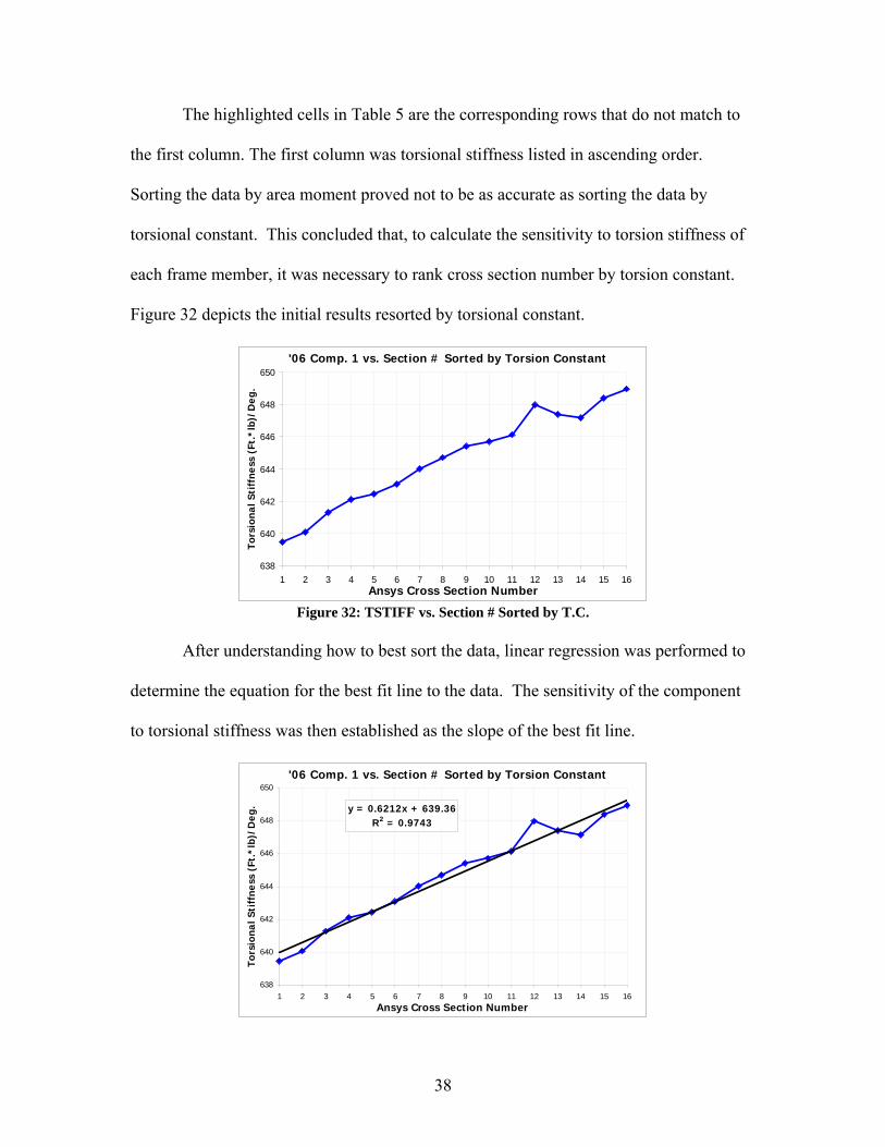
The highlighted cells in Table 5 are the corresponding rows that do not match to
the first column. The first column was torsional stiffness listed in ascending order.
Sorting the data by area moment proved not to be as accurate as sorting the data by
torsional constant. This concluded that, to calculate the sensitivity to torsion stiffness of
each frame member, it was necessary to rank cross section number by torsion constant.
Figure 32 depicts the initial results resorted by torsional constant.
'06 Comp. 1 vs. Section # Sorted by Torsion Constant
638
640
642
644
646
648
650
1 2 3 4 5 6 7 8 9 10 11 12 13 14 15 16Ansys Cross Section Number
Tors
iona
l Sti
ffne
ss (
Ft.*
lb)/
Deg
.
Figure 32: TSTIFF vs. Section # Sorted by T.C.
After understanding how to best sort the data, linear regression was performed to
determine the equation for the best fit line to the data. The sensitivity of the component
to torsional stiffness was then established as the slope of the best fit line.
'06 Comp. 1 vs. Section # Sorted by Torsion Constant
y = 0.6212x + 639.36R2 = 0.9743
638
640
642
644
646
648
650
1 2 3 4 5 6 7 8 9 10 11 12 13 14 15 16Ansys Cross Section Number
Tors
iona
l Sti
ffne
ss (
Ft.*
lb)/
Deg
.
39
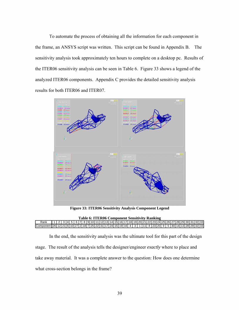
To automate the process of obtaining all the information for each component in
the frame, an ANSYS script was written. This script can be found in Appendix B. The
sensitivity analysis took approximately ten hours to complete on a desktop pc. Results of
the ITER06 sensitivity analysis can be seen in Table 6. Figure 33 shows a legend of the
analyzed ITER06 components. Appendix C provides the detailed sensitivity analysis
results for both ITER06 and ITER07.
Figure 33: ITER06 Sensitivity Analysis Component Legend
Table 6: ITER06 Component Sensitivity Ranking
Rank 1 2 3 4 5 6 7 8 9 10 11 12 13 14 15 16 17 18 19 20 21 22 23 24 25 26 27 28 29 30 31 32 33Component 26 12 21 6 10 27 2 18 7 25 22 31 17 24 15 19 16 4 3 1 11 8 23 20 9 5 30 14 13 28 29 32 33
In the end, the sensitivity analysis was the ultimate tool for this part of the design
stage. The result of the analysis tells the designer/engineer exactly where to place and
take away material. It was a complete answer to the question: How does one determine
what cross-section belongs in the frame?
40
Optimization
In an effort to take more guess work out of designing a FSAE frame, an
automated optimization script underwent experimentation. The idea behind this script
was to eliminate all manual iterating when determining the frame design. In theory, the
optimization would analyze any ANSYS frame geometry and return the best cross section
combination for all frame members to provide the best torsional stiffness. Thus, the
ultimate frame design is created.
To begin the optimization process, all the possible combinations of cross-sections
needed to be coded. The ITER07 geometry had thirty three components that could have
sixteen different possible cross-sections, which computed to 5.4 X 1039 combinations.
The amount of time to optimize that many combinations was projected to take years. In
order to reduce the number of combinations, the top four most sensitive components to
torsional stiffness were selected, which reduce the number of combinations to 65,536.
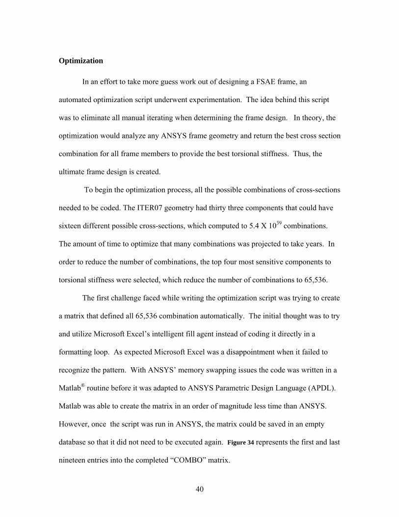
The first challenge faced while writing the optimization script was trying to create
a matrix that defined all 65,536 combination automatically. The initial thought was to try
and utilize Microsoft Excel’s intelligent fill agent instead of coding it directly in a
formatting loop. As expected Microsoft Excel was a disappointment when it failed to
recognize the pattern. With ANSYS’ memory swapping issues the code was written in a
Matlab® routine before it was adapted to ANSYS Parametric Design Language (APDL).
Matlab was able to create the matrix in an order of magnitude less time than ANSYS.
However, once the script was run in ANSYS, the matrix could be saved in an empty
database so that it did not need to be executed again. Figure 34 represents the first and last
nineteen entries into the completed “COMBO” matrix.
41
Figure 34: Optimization "COMBO" Matrix from ANSYS' Array Editor [11]
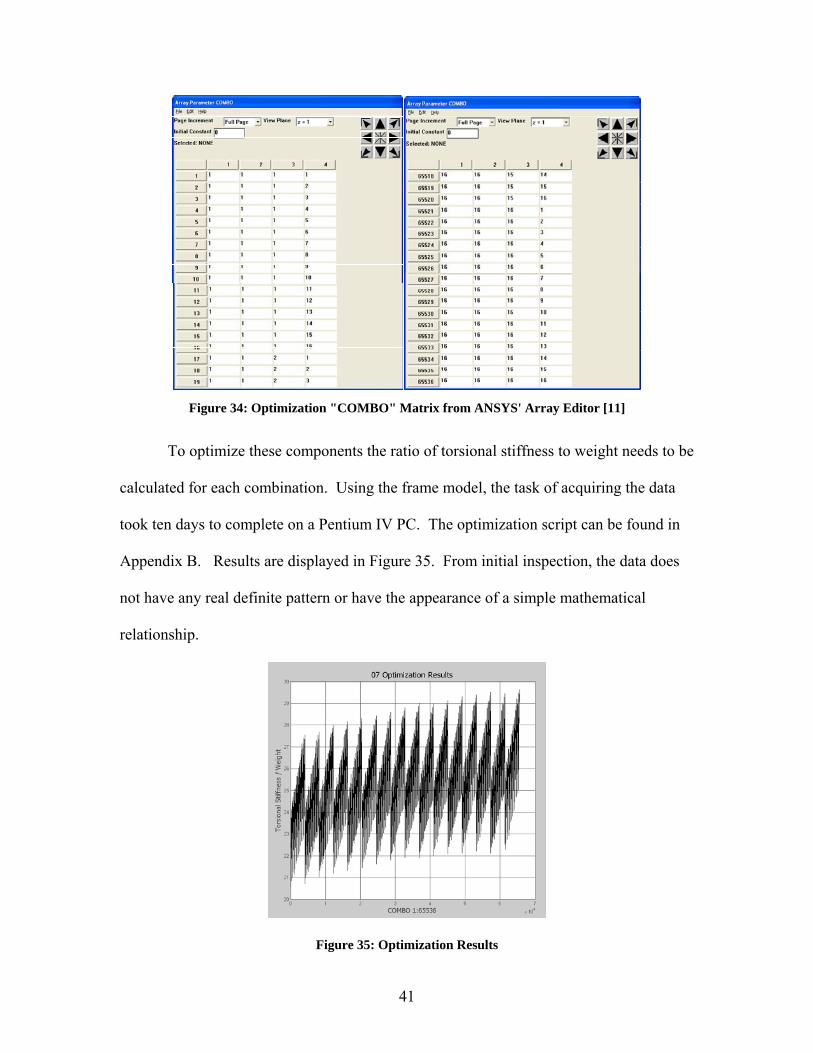
To optimize these components the ratio of torsional stiffness to weight needs to be
calculated for each combination. Using the frame model, the task of acquiring the data
took ten days to complete on a Pentium IV PC. The optimization script can be found in
Appendix B. Results are displayed in Figure 35. From initial inspection, the data does
not have any real definite pattern or have the appearance of a simple mathematical
relationship.
Figure 35: Optimization Results
42
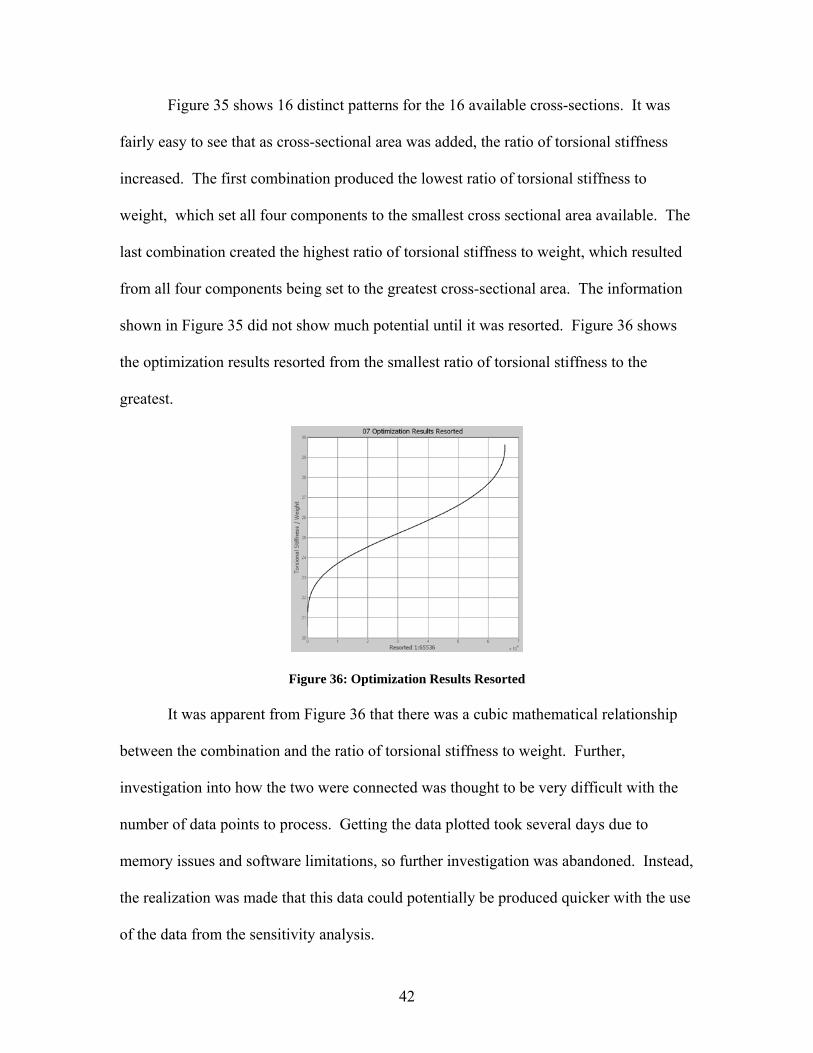
Figure 35 shows 16 distinct patterns for the 16 available cross-sections. It was
fairly easy to see that as cross-sectional area was added, the ratio of torsional stiffness
increased. The first combination produced the lowest ratio of torsional stiffness to
weight, which set all four components to the smallest cross sectional area available. The
last combination created the highest ratio of torsional stiffness to weight, which resulted
from all four components being set to the greatest cross-sectional area. The information
shown in Figure 35 did not show much potential until it was resorted. Figure 36 shows
the optimization results resorted from the smallest ratio of torsional stiffness to the
greatest.
Figure 36: Optimization Results Resorted
It was apparent from Figure 36 that there was a cubic mathematical relationship
between the combination and the ratio of torsional stiffness to weight. Further,
investigation into how the two were connected was thought to be very difficult with the
number of data points to process. Getting the data plotted took several days due to
memory issues and software limitations, so further investigation was abandoned. Instead,
the realization was made that this data could potentially be produced quicker with the use
of the data from the sensitivity analysis.
43
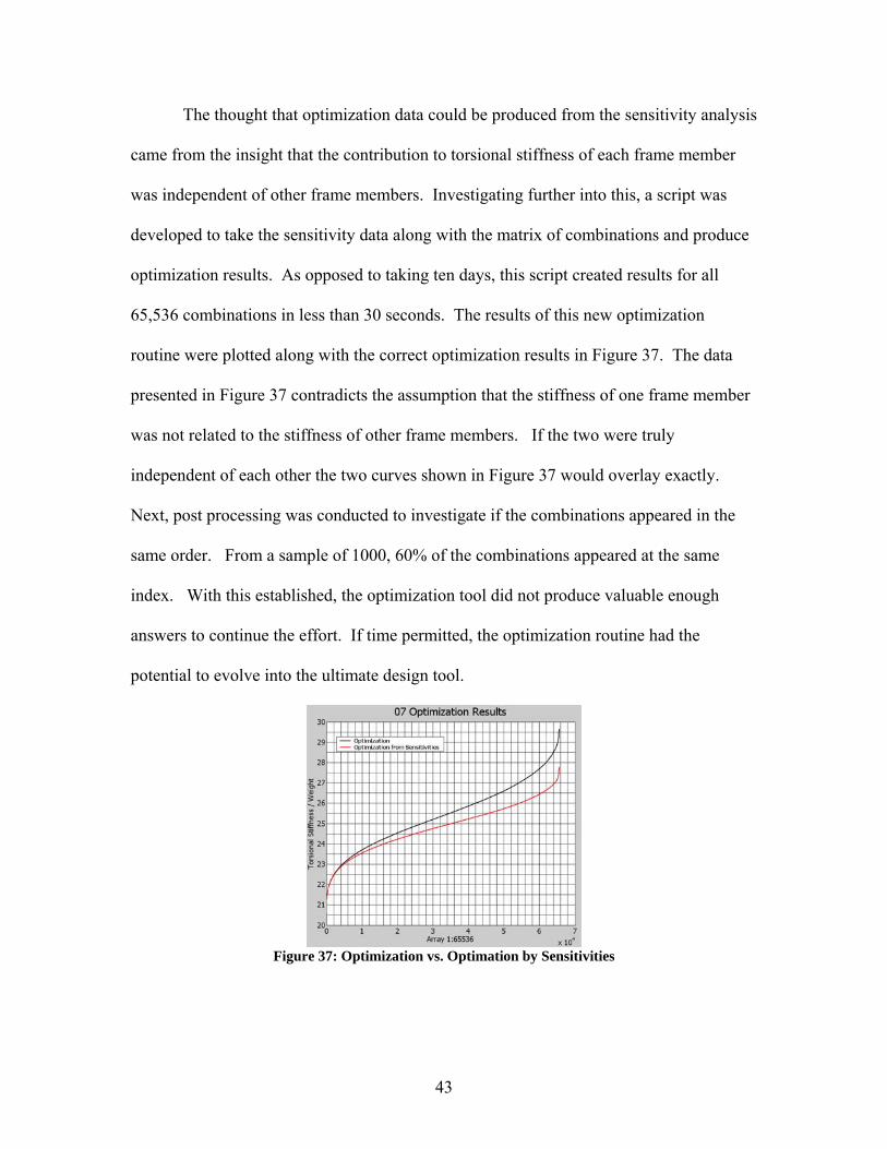
The thought that optimization data could be produced from the sensitivity analysis
came from the insight that the contribution to torsional stiffness of each frame member
was independent of other frame members. Investigating further into this, a script was
developed to take the sensitivity data along with the matrix of combinations and produce
optimization results. As opposed to taking ten days, this script created results for all
65,536 combinations in less than 30 seconds. The results of this new optimization
routine were plotted along with the correct optimization results in Figure 37. The data
presented in Figure 37 contradicts the assumption that the stiffness of one frame member
was not related to the stiffness of other frame members. If the two were truly
independent of each other the two curves shown in Figure 37 would overlay exactly.
Next, post processing was conducted to investigate if the combinations appeared in the
same order. From a sample of 1000, 60% of the combinations appeared at the same
index. With this established, the optimization tool did not produce valuable enough
answers to continue the effort. If time permitted, the optimization routine had the
potential to evolve into the ultimate design tool.
Figure 37: Optimization vs. Optimation by Sensitivities
44
Chapter 6 Torsional Stiffness Measuring Machine (TSMM)
The Torsional Stiffness Measuring Machine culminated from a need for the
experimental measurement of chassis stiffness. Research showed some very basic ideas
of how to go about taking this measurement. Some engineers chose to create their own
fixtures to hold the frame and some methods were of the “backyard” variety.
Commercially available systems are referre to as “Kinematic and Compliance Systems.”
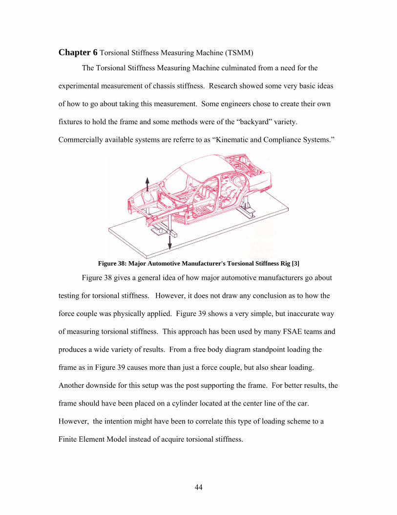
Figure 38: Major Automotive Manufacturer's Torsional Stiffness Rig [3]
Figure 38 gives a general idea of how major automotive manufacturers go about
testing for torsional stiffness. However, it does not draw any conclusion as to how the
force couple was physically applied. Figure 39 shows a very simple, but inaccurate way
of measuring torsional stiffness. This approach has been used by many FSAE teams and
produces a wide variety of results. From a free body diagram standpoint loading the
frame as in Figure 39 causes more than just a force couple, but also shear loading.
Another downside for this setup was the post supporting the frame. For better results, the
frame should have been placed on a cylinder located at the center line of the car.
However, the intention might have been to correlate this type of loading scheme to a
Finite Element Model instead of acquire torsional stiffness.
45
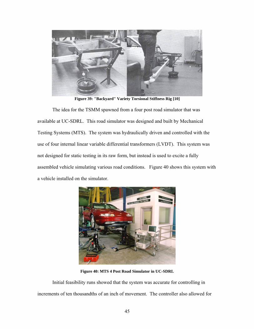
Figure 39: "Backyard" Variety Torsional Stiffness Rig [10]
The idea for the TSMM spawned from a four post road simulator that was
available at UC-SDRL. This road simulator was designed and built by Mechanical
Testing Systems (MTS). The system was hydraulically driven and controlled with the
use of four internal linear variable differential transformers (LVDT). This system was
not designed for static testing in its raw form, but instead is used to excite a fully
assembled vehicle simulating various road conditions. Figure 40 shows this system with
a vehicle installed on the simulator.
Figure 40: MTS 4 Post Road Simulator in UC-SDRL
Initial feasibility runs showed that the system was accurate for controlling in
increments of ten thousandths of an inch of movement. The controller also allowed for
46
the ability to displace each post independently. With these two capabilities established,
the TSMM concept started to become a reality. The next question that needed to be
answered was how to connect the racecar to the each of the posts.
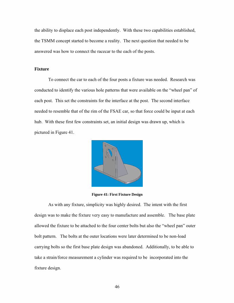
Fixture
To connect the car to each of the four posts a fixture was needed. Research was
conducted to identify the various hole patterns that were available on the “wheel pan” of
each post. This set the constraints for the interface at the post. The second interface
needed to resemble that of the rim of the FSAE car, so that force could be input at each
hub. With these first few constraints set, an initial design was drawn up, which is
pictured in Figure 41.
Figure 41: First Fixture Design
As with any fixture, simplicity was highly desired. The intent with the first
design was to make the fixture very easy to manufacture and assemble. The base plate
allowed the fixture to be attached to the four center bolts but also the “wheel pan” outer
bolt pattern. The bolts at the outer locations were later determined to be non-load
carrying bolts so the first base plate design was abandoned. Additionally, to be able to
take a strain/force measurement a cylinder was required to be incorporated into the
fixture design.

47
Figure 42: Second Fixture Design The first design being inadequate led to the design shown in Figure 42. This design was
improved with the integration of a cylinder and the redesign of the base plate to only
capture the four bolts at the center of each post. However, after more discussion and
thought, flaws were again revealed. They began with the fact that there was the potential
for a lot of bending stress if there were to be any misalignment. The nature of the cars’
suspension systems was to have camber change as the wheel moved vertically. The
second fixture design would constrain this motion, leading to some potential load
magnification. Lastly, the need for a mechanical fuse was desired to prevent yielding of
any suspension components. To remedy these major flaws, a pivot was integrated into
the design along with a mechanical fuse.
48
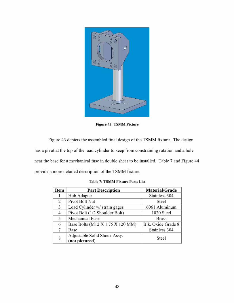
Figure 43: TSMM Fixture
Figure 43 depicts the assembled final design of the TSMM fixture. The design
has a pivot at the top of the load cylinder to keep from constraining rotation and a hole
near the base for a mechanical fuse in double shear to be installed. Table 7 and Figure 44
provide a more detailed description of the TSMM fixture.
Table 7: TSMM Fixture Parts List
Item Part Description Material/Grade 1 Hub Adapter Stainless 304 2 Pivot Bolt Nut Steel 3 Load Cylinder w/ strain gages 6061 Aluminum 4 Pivot Bolt (1/2 Shoulder Bolt) 1020 Steel 5 Mechanical Fuse Brass 6 Base Bolts (M12 X 1.75 X 120 MM) Blk. Oxide Grade 8 7 Base Stainless 304
8 Adjustable Solid Shock Assy. (not pictured) Steel
49
1
23
4
56
7
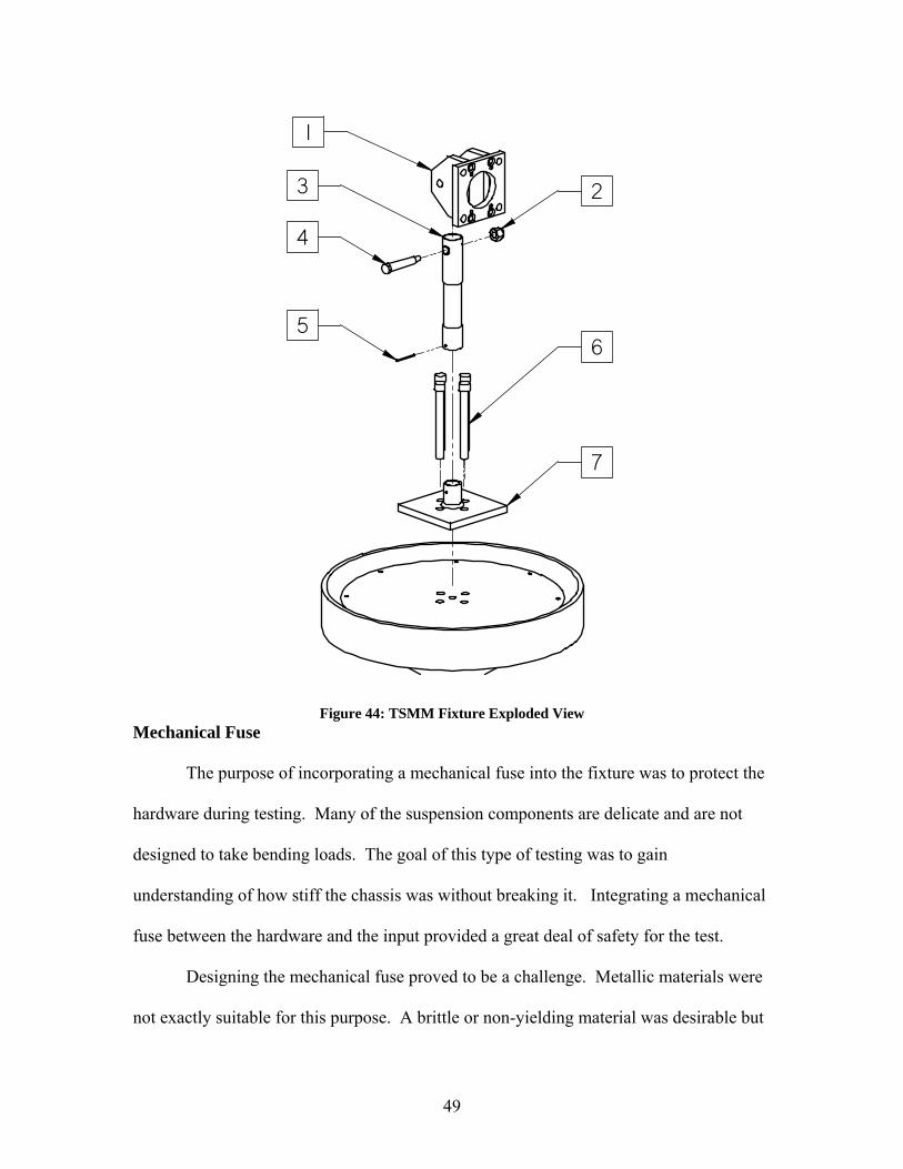
Figure 44: TSMM Fixture Exploded View Mechanical Fuse
The purpose of incorporating a mechanical fuse into the fixture was to protect the
hardware during testing. Many of the suspension components are delicate and are not
designed to take bending loads. The goal of this type of testing was to gain
understanding of how stiff the chassis was without breaking it. Integrating a mechanical
fuse between the hardware and the input provided a great deal of safety for the test.
Designing the mechanical fuse proved to be a challenge. Metallic materials were
not exactly suitable for this purpose. A brittle or non-yielding material was desirable but
50
was difficult to locate in a form that could quickly be manufactured. Searching material
supplier databases returned little-to-no results for raw forms of ceramic materials.
Reluctantly, the choice to use brass was made. Brass was chosen because of its low
shear strength and availability. As a backup, nylon was thought to be a second choice if
brass were to become a problem.
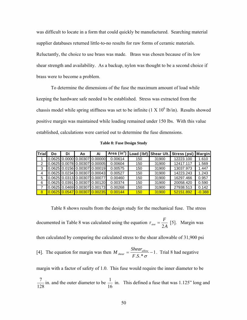
To determine the dimensions of the fuse the maximum amount of load while
keeping the hardware safe needed to be established. Stress was extracted from the
chassis model while spring stiffness was set to be infinite (1 X 10⁶ lb/in). Results showed
positive margin was maintained while loading remained under 150 lbs. With this value
established, calculations were carried out to determine the fuse dimensions.
Table 8: Fuse Design Study Trial Do Di Ao Ai Area (in2) Load (lbf) Shear Ult. Stress (psi) Margin
1 0.0625 0.0000 0.00307 0.00000 0.00614 150 31900 12223.100 1.6102 0.0625 0.0078 0.00307 0.00005 0.00604 150 31900 12417.117 1.5693 0.0625 0.0156 0.00307 0.00019 0.00575 150 31900 13037.973 1.4474 0.0625 0.0234 0.00307 0.00043 0.00527 150 31900 14223.243 1.2435 0.0625 0.0313 0.00307 0.00077 0.00460 150 31900 16297.466 0.9576 0.0625 0.0391 0.00307 0.00120 0.00374 150 31900 20058.420 0.5907 0.0625 0.0469 0.00307 0.00173 0.00268 150 31900 27938.513 0.1428 0.0625 0.0547 0.00307 0.00235 0.00144 150 31900 52151.892 -0.388
Table 8 shows results from the design study for the mechanical fuse. The stress
documented in Table 8 was calculated using the equation A
Fave 2
=τ [5]. Margin was
then calculated by comparing the calculated stress to the shear allowable of 31,900 psi
[4]. The equation for margin was then 1*..
−=σSF
ShearM allow
shear . Trial 8 had negative
margin with a factor of safety of 1.0. This fuse would require the inner diameter to be
1287 in. and the outer diameter to be
161 in. This defined a fuse that was 1.125” long and
51
had a wall thickness of 0.003”. Machining a fuse with this small of a wall thickness
seemed very unrealistic.
When material for the mechanical fuse arrived, manual machining of an internal
diameter proved to be almost impossible. Directing a drill bit through a 1/16” diameter
stock of yellow brass, with the help of a center drill proved to be extremely difficult.
Any wobbling of the drill bit or weakening of the part caused it to shear immediately
from the lathe. Eventually, the idea for boring out the 1/16” diameter brass stock was
abandoned after a few tries. The backup nylon fuse was then tested as a result of the
failure to create the ideal brass fuse. Experimental testing of the nylon fuse showed that
it would fail around 100 lbs of load. Testing commenced with the nylon fuse.
52
Strain Gauge Setup
With the fuse determined, attention was turned to how to setup the strain gauges
so that the axial load could be logged during testing. The strain gauges needed to be
wired in a manner that would ignore any bending stress that the load cylinder
experienced.
Figure 45: Strain Gauge Setup [6]
Using the setup described by Figure 45, bending stresses could be neglected.
Two strain gauges were placed diametrically opposite of each other. [6] The two gages
were then wired in series and installed in one leg of a wheatstone bridge.
Figure 46: Bending, Tension, & Combined [6]
Perry and Lisner describe, “ It is apparent from this illustration (Figure 42) that if the
shank is being bent slightly by non-axial loading, gage A will ‘feel’ a strain somewhat
greater than the uniform strain representative of pure tension. On the other hand, the net
strain felt by gage B will be lower than it should be by exactly the same amount. If these
gages are placed in series electrically, the circuit effectively adds their results and divides
by two, which gives the true tensile strain and eliminates all the strain indication due to
bending.” [6]
53
Strain Gage Installation
Installing the strain gages on the load cylinders was again no easy task. It
required an extreme amount of patience and discipline for following directions. Any step
left out led to the strain gage being pulled from the part and discarded. At $7 each, it was
very important to complete each step properly. A complete step-by-step installation
guide can be found for each individual brand of strain gage. Vishay strain gauges were
used for testing and their step by step installation guide can be found in Reference 7.
Strain Gage Wiring
With all the strain gages installed on the load cylinders, attention was focused on
how to properly wire both the strain gages and the strain gage conditioner. A quarter
bridge was required for this type of setup. To begin the installation of the two strain
gages in series, a jumper cable was installed to connect the two. Both the P- and S- wires
are soldered together at one of the relief pads and the remaining P+ wire was soldered to
the last vacant solder pad on the opposite strain gage. For better clarity, reference the
wiring schematic in Figure 47 below.
Figure 47: Strain Gage Wiring Schematic
Wiring the Vishay Strain Gage Conditioner and Amplifier system for the quarter
bridge circuit came next. Previously, the system was configured for a full bridge circuit.
Pinning-out each strain gage amplifier connector took some time. Soldering the
54
terminals was difficult due to the limited access the connector design provides to the pins.
As with any process, it became easier with practice. The key was to keep the heat on the
pin and not the wire. Once the pin was hot enough the old solder would melt and the
wire could be inserted. With the addition of each wire, it was important to keep the
soldering tip away, so that insulation did not melt. It was also a good practice to keep a
set of safety glasses on while soldering. Figure 48 is a modified schematic from the
Vishay Conditioner Instruction Manual, Reference 8.
Figure 48: Strain Gage Conditioner Pin Out Schematic [8]
As the diagram describes, it was necessary to wire an extra resistor in line with
the P- signal. The size of the resistor needed to be equal to the total resistance of the two
strain gages in series. This created the second arm of the bridge circuit that balances the
arm containing the two strain gages. For example, if both strain gage A & B were 350 Ω,
the total resistance needed would be 700 Ω. Therefore, the resistance in the second arm
of the bridge needed to balance this resistance, by also having 700 Ω of resistance. This
could be achieved through two methods. Method one was to wire a 700 Ω precision
resistor at the dummy resistor location, according to Figure 47. The second method was
to install a 350 Ω precision resistor at the dummy resistor location and wire this lead to
the G pin in Figure 48. Wiring to the G pin uses an internal precision 350 Ω resistor
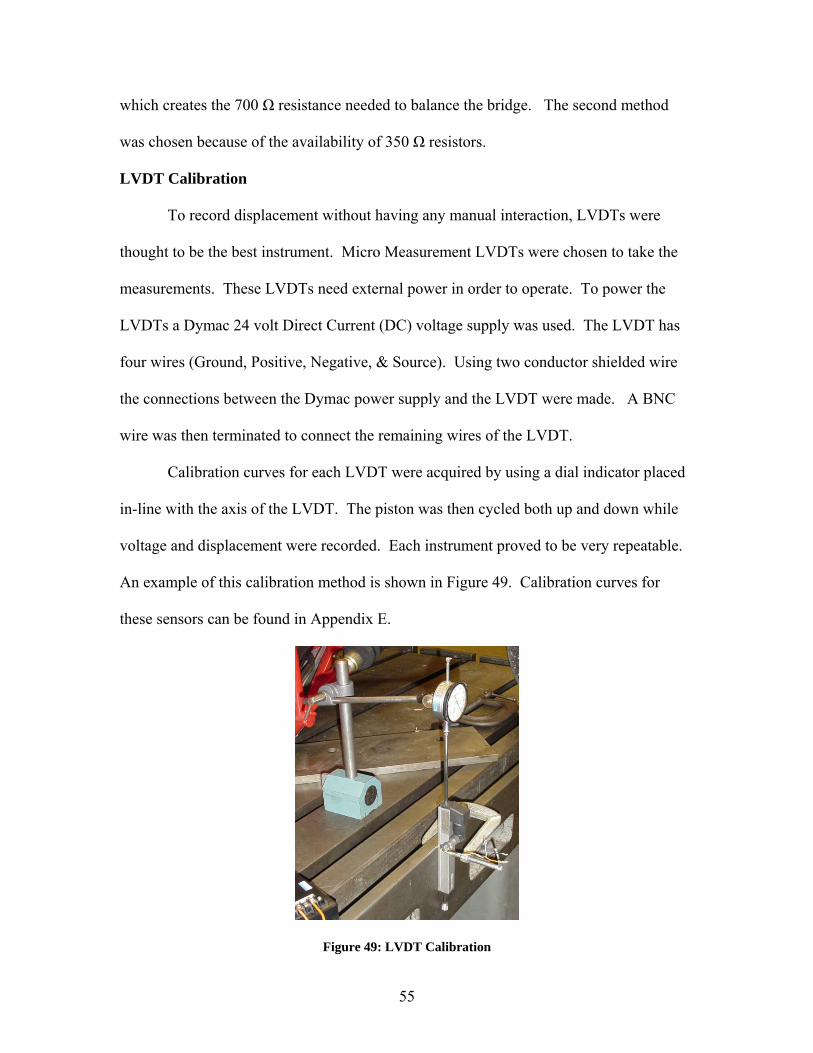
55
which creates the 700 Ω resistance needed to balance the bridge. The second method
was chosen because of the availability of 350 Ω resistors.
LVDT Calibration
To record displacement without having any manual interaction, LVDTs were
thought to be the best instrument. Micro Measurement LVDTs were chosen to take the
measurements. These LVDTs need external power in order to operate. To power the
LVDTs a Dymac 24 volt Direct Current (DC) voltage supply was used. The LVDT has
four wires (Ground, Positive, Negative, & Source). Using two conductor shielded wire
the connections between the Dymac power supply and the LVDT were made. A BNC
wire was then terminated to connect the remaining wires of the LVDT.
Calibration curves for each LVDT were acquired by using a dial indicator placed
in-line with the axis of the LVDT. The piston was then cycled both up and down while
voltage and displacement were recorded. Each instrument proved to be very repeatable.
An example of this calibration method is shown in Figure 49. Calibration curves for
these sensors can be found in Appendix E.
Figure 49: LVDT Calibration
56
Testing
There were many challenges that were overcome during the first session of
testing. The most important challenge was to determine the order in which events should
occur. The ITER06 chassis was installed on the fixture first without installing the solid
shocks beforehand (a rigid shock allowed for a direct calculation of stiffness of the frame
and suspension components alone.) While installing the solid shocks on the fixture, the
ITER06 chassis was overloaded and a lower front a-arm was bent. With the order of
events re-worked, ITER05 chassis was installed next. Solid shocks were installed prior
to installing the chassis on the TSMM. The sequence to installing each post was
documented and can found in the procedure in Appendix G. The order in which these
events needed to occur was critical to the chassis’ safety.
During the first test session using the ITER06 chassis, conclusions about the fuse
and the ability to control the angle of twist were drawn. Initially, the ITER06 chassis was
installed using the plastic mechanical fuses. The load applied to the chassis during
testing was mostly absorbed by the elasticity of the plastic fuse. After a few data points
were collected the fuses were replaced with the solid brass mechanical fuses. The brass
fuses showed no signs of bowing/sinking. However, the brass fuses being solid, the
“fuse” characteristic was lost. Knowing that the controller was accurate in moving in ten
thousandths of an inch and having a dynamic display of the load, this was not a huge
concern. Testing of the ITER05 chassis completed with no harm to the hardware.
For each chassis tested, two approaches were made. The first approach was to
move the front two posts in increments of 0.020”, followed by a second test using 0.050”
increments. The initial theory was that testing with 0.020” increments would allow the
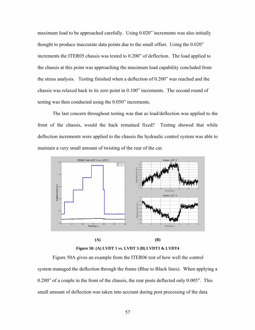
57
maximum load to be approached carefully. Using 0.020” increments was also initially
thought to produce inaccurate data points due to the small offset. Using the 0.020”
increments the ITER05 chassis was tested to 0.200” of deflection. The load applied to
the chassis at this point was approaching the maximum load capability concluded from
the stress analysis. Testing finished when a deflection of 0.200” was reached and the
chassis was relaxed back to its zero point in 0.100” increments. The second round of
testing was then conducted using the 0.050” increments.
The last concern throughout testing was that as load/deflection was applied to the
front of the chassis, would the back remained fixed? Testing showed that while
deflection increments were applied to the chassis the hydraulic control system was able to
maintain a very small amount of twisting of the rear of the car.
(A) (B)
Figure 50: (A) LVDT 1 vs. LVDT 3 (B) LVDT3 & LVDT4
Figure 50A gives an example from the ITER06 test of how well the control
system managed the deflection through the frame (Blue to Black lines). When applying a
0.200” of a couple in the front of the chassis, the rear posts deflected only 0.005”. This
small amount of deflection was taken into account during post processing of the data.
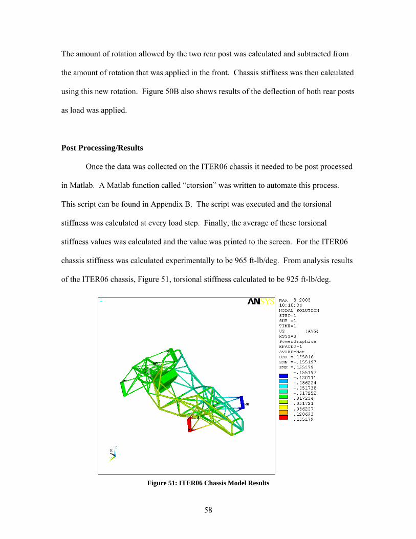
58
The amount of rotation allowed by the two rear post was calculated and subtracted from
the amount of rotation that was applied in the front. Chassis stiffness was then calculated
using this new rotation. Figure 50B also shows results of the deflection of both rear posts
as load was applied.
Post Processing/Results
Once the data was collected on the ITER06 chassis it needed to be post processed
in Matlab. A Matlab function called “ctorsion” was written to automate this process.
This script can be found in Appendix B. The script was executed and the torsional
stiffness was calculated at every load step. Finally, the average of these torsional
stiffness values was calculated and the value was printed to the screen. For the ITER06
chassis stiffness was calculated experimentally to be 965 ft-lb/deg. From analysis results
of the ITER06 chassis, Figure 51, torsional stiffness calculated to be 925 ft-lb/deg.
Figure 51: ITER06 Chassis Model Results
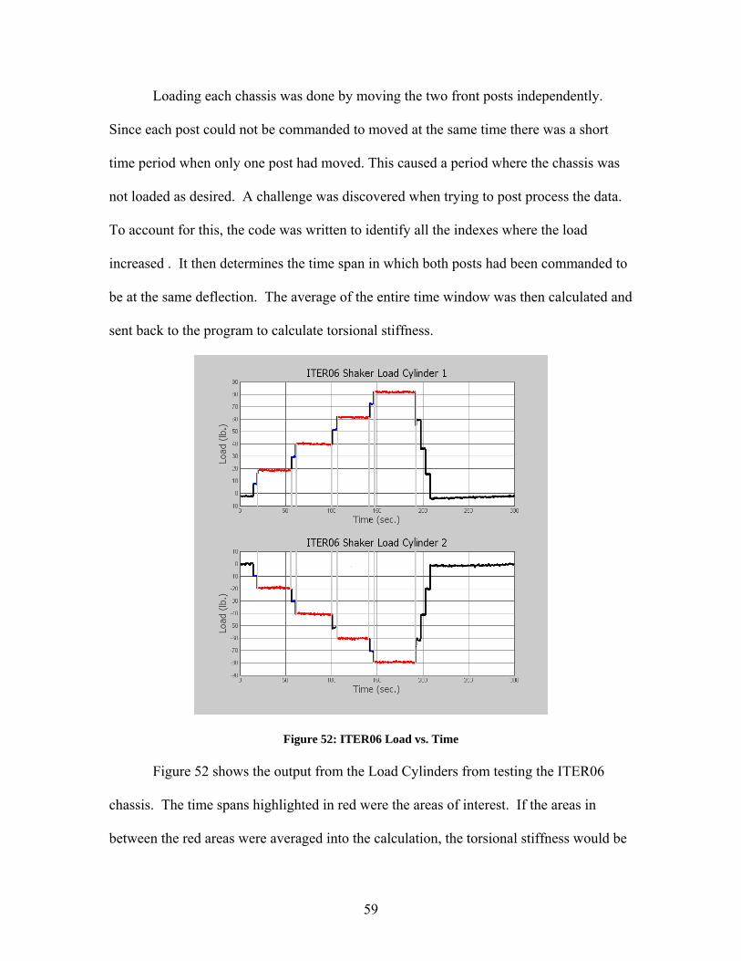
59
Loading each chassis was done by moving the two front posts independently.
Since each post could not be commanded to moved at the same time there was a short
time period when only one post had moved. This caused a period where the chassis was
not loaded as desired. A challenge was discovered when trying to post process the data.
To account for this, the code was written to identify all the indexes where the load
increased . It then determines the time span in which both posts had been commanded to
be at the same deflection. The average of the entire time window was then calculated and
sent back to the program to calculate torsional stiffness.
Figure 52: ITER06 Load vs. Time
Figure 52 shows the output from the Load Cylinders from testing the ITER06
chassis. The time spans highlighted in red were the areas of interest. If the areas in
between the red areas were averaged into the calculation, the torsional stiffness would be
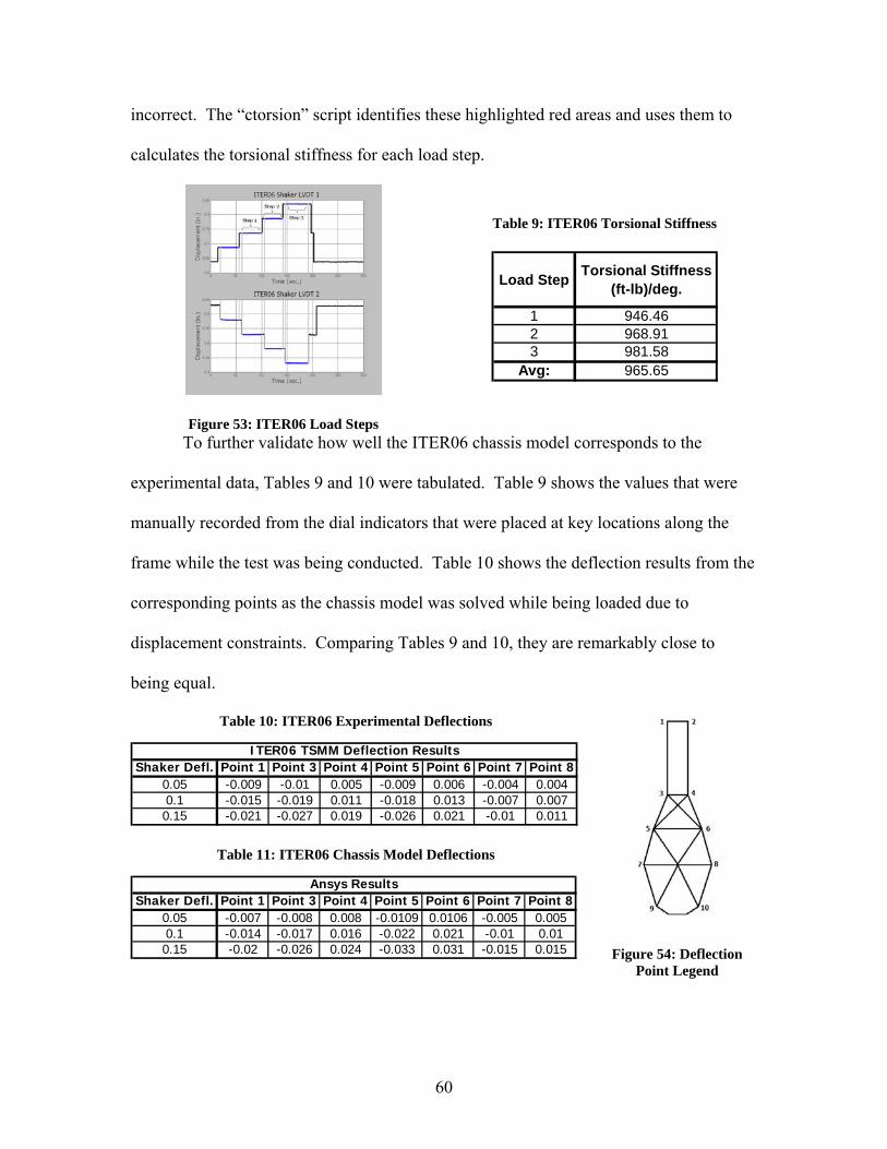
60
incorrect. The “ctorsion” script identifies these highlighted red areas and uses them to
calculates the torsional stiffness for each load step.
Figure 53: ITER06 Load Steps
Table 9: ITER06 Torsional Stiffness
Load Step Torsional Stiffness (ft-lb)/deg.
1 946.462 968.913 981.58
Avg: 965.65
To further validate how well the ITER06 chassis model corresponds to the
experimental data, Tables 9 and 10 were tabulated. Table 9 shows the values that were
manually recorded from the dial indicators that were placed at key locations along the
frame while the test was being conducted. Table 10 shows the deflection results from the
corresponding points as the chassis model was solved while being loaded due to
displacement constraints. Comparing Tables 9 and 10, they are remarkably close to
being equal.
Table 10: ITER06 Experimental Deflections
ITER06 TSMM Deflection ResultsShaker Defl. Point 1 Point 3 Point 4 Point 5 Point 6 Point 7 Point 8
0.05 -0.009 -0.01 0.005 -0.009 0.006 -0.004 0.0040.1 -0.015 -0.019 0.011 -0.018 0.013 -0.007 0.0070.15 -0.021 -0.027 0.019 -0.026 0.021 -0.01 0.011
Table 11: ITER06 Chassis Model Deflections
Ansys ResultsShaker Defl. Point 1 Point 3 Point 4 Point 5 Point 6 Point 7 Point 8
0.05 -0.007 -0.008 0.008 -0.0109 0.0106 -0.005 0.0050.1 -0.014 -0.017 0.016 -0.022 0.021 -0.01 0.010.15 -0.02 -0.026 0.024 -0.033 0.031 -0.015 0.015
Figure 54: Deflection Point Legend
61
Chapter 7 Conclusion / Future Recommendations
Conclusion
For Formula SAE teams it is not only a race to the finish line, but also a race to
finish the building and validation of a racecar. Having every tool possible to “get there”
gives teams the upper advantage. The design and validation of the chassis as a whole
will continue to be the focal point at every collegiate racecar competition. Understanding
and utilizing the tools presented in the preceding will not only speed the process, but will
also provide that extra edge for competition.
The process from frame to chassis model is an engineering process that has been
proven to work at the University of Cincinnati. Establishing and documenting this
process will allow future teams to achieve the goals they have for their designs.
Following this process also allows for a direct comparison from year-to-year. When rule
changes are so widespread that a year-to-year comparison can not be made, engineers can
find reassurance that if this process is followed, the result will be a very good working
product. This process gives excellent trend (relative) information to evaluate progress as
well as accurate absolute (properly scaled) numbers for ultimate design and analysis.
The automation of the sensitivity analysis played a key role in the success of this
process for the UC Formula SAE team. Having a global view of how each tube’s
stiffness contributed to the overall stiffness of the frame was a huge step forward in the
design process. The ability to quickly make changes as manufacturing issues arose was
an invaluable asset. The sensitivity analysis tool saved time by pointing the designer in
the direction that needed to be taken in order to improve frame stiffness. In the end, this
allowed for more time to be dedicated to the building and manufacturing and assembly of

62
the vehicle. The sensitivity analysis proved not only to be a great tool for this type of
design work but it also has the potential to be adapted to aid in the design of any
structure.
In the end, the optimization tool presented did not turn out to be the ultimate
design tool. The number of combinations needing to be solved in such a short period of
time overwhelmed the idea. However, the results of the small subset that was evaluated
showed great potential. To have absolutely no human interaction required to complete
the design of the frame would be a tremendous feat of ingenuity. It would, without a
doubt, give any team the upper hand. With advancements in CPU speed and a more
robust code, this tool could quickly become a very valuable engineering tool.
Testing and validation is an important part of any engineering process. Testing
allows engineers to prove not only to themselves but to others, that what was designed is
that which was built. Having a test rig such as the TSMM allows for a direct comparison
from model to hardware. Comparing the data from the rig to analytical data showed that
the correct loading scheme was achieved. The results of torsional stiffness showed that it
can produce very accurate answers. This gives confirmation that the actual hardware will
perform as it was designed to. Results boost team confidence and gives reassurance that
the chassis can make it to the finish line. Having this testing process established plays a
large role in communicating with design judges in a collegiate competition. The ability
to relay that a $500,000 four post dynamic shaker system was modified to statically
measure chassis torsional stiffness is an impressing and interesting conversation starter.
Having a test rig like the TSMM, shows design judges that your design innovation does
not just stop at the car, but is continued into accurate testing and validation methods.
63
This also justifies that future designs can proceed analytically with only minimal testing
and validation.
Design Tools
Beyond the design tools presented there is much more to consider. A script could
be developed to automatically take a Solid Edge model and turn it into a working
ANSYS frame model. The leap between the frame model to the chassis model would be
much more difficult. With the help of a Matlab GUI, it could be achieved. The notion of
having a set of points loaded into a Matlab GUI and then formatted into an ANSYS
database is very possible. The result would yield an entirely automated process, start to
finish, eliminating the need for the more complicated processes outlined in Chapters 2
and 3.
If the choice to completely automate the analysis process from Solid Edge to
ANSYS is not chosen, the recommended path is to make the solution routines a little
more user friendly. This could be completed with the use of a feature in ANSYS. The
scripts can be added in as a command in the toolbar. The result would be such that each
time the ANSYS GUI is opened, the commands to run the scripts are only one click
away.
The most difficult tool to write would be a geometry optimizer. The scripts
presented in this text do not take into account that, between the defined points, the
arrangement of tubes could be different. A script could be written to identify whether it
is more important for a frame member to be oriented at one angle versus another. A
script of this nature could be derived from the sensitivity routine. Components could be

64
defined such that at times they are meshed and at others, are not. This would measure the
difference in torsional stiffness with and without this component in the frame.
Additionally, the link between modal analysis and experimental modal analysis
could be better defined with the help of a cross-orthogonality script. This script would
extract the modal vectors (mode shapes) of the analysis and do the same for the
experimental data. These two vector pairs can then be compared for each mode and a
better understanding of how well the analysis actually compared to experimental data.
Once the set of vectors are defined for each mode they can be compared for how parallel
they are. This would be the ultimate modal analysis correlation tool.
The Taguchi Method could also be implemented to help optimize the frame. The
Taguchi Method was developed to optimize manufacturing processes, however it could
be adapted to perform case studies on the frame. The Taguchi method utilizes orthogonal
arrays. Orthogonal arrays are tables which define a minimum number of experiments to
be able to understand the importance of one parameters versus another. When the data
has been collected, signal to noise ratios are calculated for each parameter. The
parameters with the largest signal to noise ratios are then considered more important [4].
Another optimization process that could considerably improve the frame design
would be to implement the use of objective functions. A function could be developed,
along with a set of inequalities, that when solved using differential calculus could
generate the optimal frame design [15]. An example problem using objective functions
has been illustrated in Chapter 2 of Reference 15. This optimization technique was also
found to be in current Finite Element (F.E.) Programs and should be investigated to
determine its value in improving future frame designs.
65
Torsional Stiffness Measuring Machine
The TSMM was designed and built because it is extremely versatile and possesses
opportunities for improvement. There are some basic upgrades that could be made and
some extensive ones. All of these upgrades should be completed to better understand the
ability of the chassis to do its job and perform at its peak.
To begin, there are various minor modifications that should be made to the rig.
First, the holes that were created in the base of the each fixture were reamed to the size of
the fixture bolts. These bolts when purchased were bowed. This did not allow for a very
easy installation. There are two options that could be executed that would easily remedy
this situation. Better grade bolts could be purchased or the sixteen holes could be reamed
out with an over-sized reamer. Knowing that the bolts of this type, length and grade are
expensive, the recommended way is to use the over-sized reamer.
The solid shocks designed for the TSMM were difficult to use because the correct
rod ends were not available. Therefore, thin spacers needed to be created to hold the
center-line of the solid shock at the correct height. Trying to install two spacers above
and below the rod end inside the frame pickup tube presented a frustrating challenge. For
the future, it is recommended that, each year, a custom set of solid shocks be made at the
correct width of the shock mating interface. The other option would be to make a
tapered sliding dovetail joint that could be adjusted for length and locked at the correct
height. Depending on the construction of this joint, it may pose problems while testing.
The dovetail could potentially slip if it is not pinned. The recommended way to fix this
issue is to make a custom set of solid shocks. Each year, a solid shock assembly should
66
be an automatic item to be fabricated by the suspension team. This solid shock assembly
should be designed to be integrated into the TSMM.
To increase the confidence in the results of the TSMM data, an easy upgrade
would be to acquire some steel pins to replace the “fuse” in the fixture. The solid brass
fuses performed without any indication of yielding. However, the fuses were under
constant load when vehicles were attached to the rig. Replacing these fuses with a
material that has a higher shear modulus would be recommended.
For testing, a great addition to the TSMM would be to connect the two forward
posts to move in unison with one button press of the controller. This would eliminate the
pause from the movement sequence of each front post. Inherently, this would eliminate
the need to identify the correct time period in which both post have been moved. In order
to accomplish this, internal coding in the hydraulic controller software may be required.
This would probably involve some heavy “C” coding and would take quite a few months
to integrate. A better solution would be to go back to the software design group and ask
if this option could be added into the next revision of the software.
The TSMM was conceptualized and built to have many more capabilities than just
a torsional stiffness measuring rig. The rig is capable of being setup to test suspension
parameters. If a table was designed and built to hold the frame fixed, a single post could
be translated while suspension parameters are measured. This type of testing eliminates
the use of solid shocks and poses less harm to the car. This test would replace the need to
travel to Goodyear to utilize their suspension parameter measuring machine and would
give the Formula team that much more time to understand the current suspension design.
Having built and designed a suspension parameter measuring machine would also

67
provide more justification that the Formula Team understands the suspension and how it
is suppose to perform, when presenting to the competition judges. The rig would need
some modification to accomplish this. A three point sensor system would need to be
developed. This could be done with the use of string potentiometers or perhaps a laser
tracking system. In addition, a kinematic table would need to be developed to pitch and
yaw the frame. The cost of materials and sensors to create this addition would probably
overwhelm the budget and consume valuable design time. The system would take many
years to develop. The software alone to process and create the curves would require the
suspension team leader’s time and some heavy Matlab code training.
The more desirable addition would be to use the TSMM rig as a quick way to
simulate on track conditions if weather or track availability presented issues. A Motec
data acquisition system was purchased in 2007 for acquiring on track data. Information
from the Motec data acquisition system could be used to produce a time history of
displacement at each wheel. This data could be formatted as input into the four post
simulation software. With the input established the simulation could be run and team
members could closely monitor chassis performance. During the simulation, strain gauge
information could be logged on any part of the vehicle. This would also provide the
chance for team members to check operating clearances, which could warrant design
changes and prevent hardware failure.
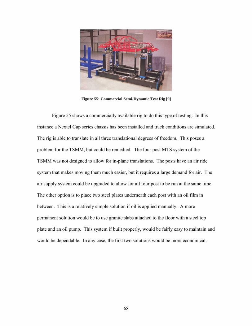
68
Figure 55: Commercial Semi-Dynamic Test Rig [9]
Figure 55 shows a commercially available rig to do this type of testing. In this
instance a Nextel Cup series chassis has been installed and track conditions are simulated.
The rig is able to translate in all three translational degrees of freedom. This poses a
problem for the TSMM, but could be remedied. The four post MTS system of the
TSMM was not designed to allow for in-plane translations. The posts have an air ride
system that makes moving them much easier, but it requires a large demand for air. The
air supply system could be upgraded to allow for all four post to be run at the same time.
The other option is to place two steel plates underneath each post with an oil film in
between. This is a relatively simple solution if oil is applied manually. A more
permanent solution would be to use granite slabs attached to the floor with a steel top
plate and an oil pump. This system if built properly, would be fairly easy to maintain and
would be dependable. In any case, the first two solutions would be more economical.
69
References
1. Aird, Forbes. Race Car Chassis: Design and Construction. Osceola:MBI, 1997 2. Sakkis, Tony. Anatomy & Development of the Indy Car. Osceola: MBI, 1994 3. Weissler, Paul “Body by the numbers.” Automotive Engineering International Sep. 2007: 26+ 4. Roy, Ranjit. A Primer on the Taguchi Method. Dearborn, MI: Society of Manufacturing
Engineers, 1990 5. Beer, Ferdinand, E. Johnson, and John DeWolf. Mechanics of Materials. New York, NY:
McGraw Hill, 2001.
6. Perry, C., and H. R. Lissner. The Strain Gage Primer. New York, NY: McGraw Hill, 1962
7. Student Manual for Strain Gage Technology. Raleigh: North Carolina, 1992
8. Strain Gage Conditioner and Amplifier System Instruction Manual. Raleigh: North Carolina:
TD, 1992.
9. Monaghan, Matt “New Simulation Rig Help ‘Tighten’ Racecar Performance.” Automotive Engineering International Dec. 2007: 62-63
10. Adams, Herb. Chassis Engineering. New York, NY: HP Books, 1993 11. ANSYS Academic Research, v. 8.0 12. ANSYS Academic Research,8.0, Help System, Command Reference, ANSYS Inc. 13. ANSYS Academic Research 8.0, Help System, Element Reference, ANSYS, Inc. 14. Solid Edge Academic ,V17 15. Haftka, Raphael and Zafer Gϋrdal. Elements of Structural Optimization. Dordrecht,
Netherlands: Kluwer, 1992
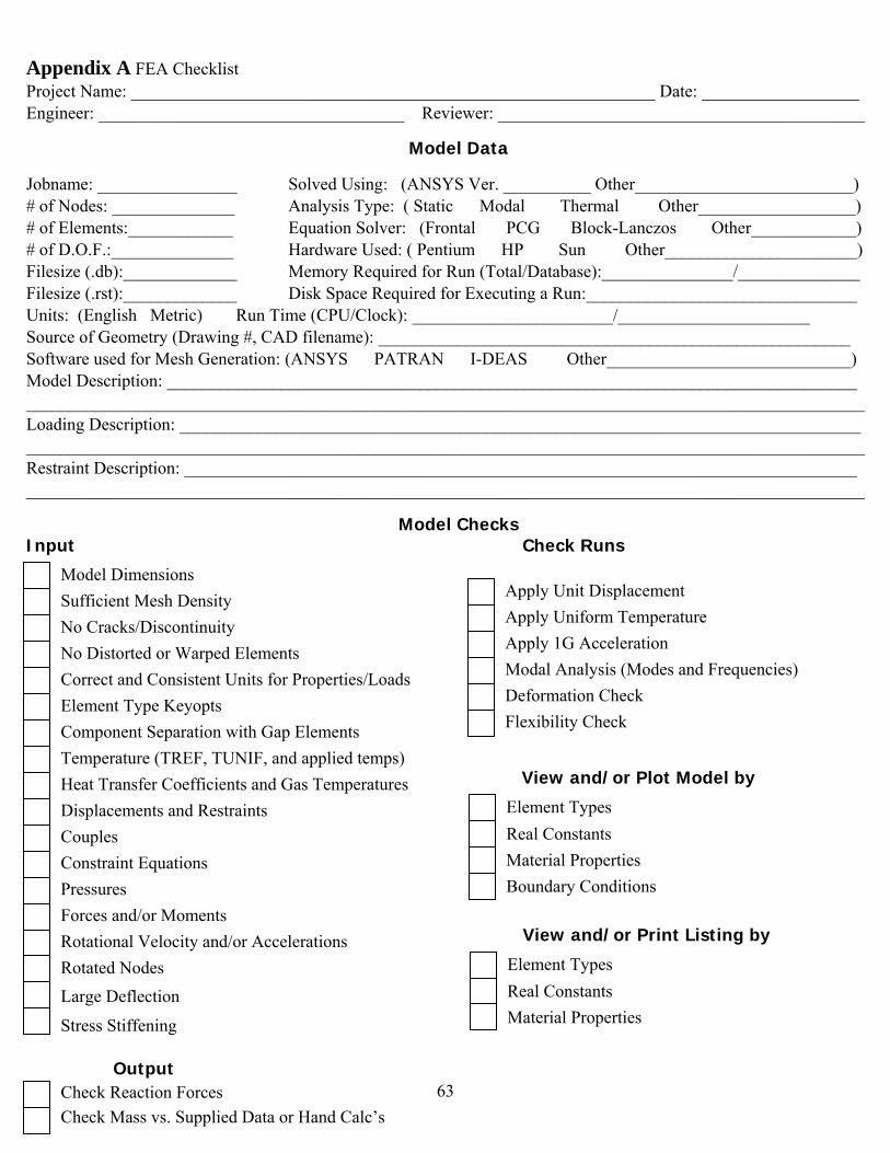
63
Model Dimensions Sufficient Mesh Density No Cracks/Discontinuity No Distorted or Warped Elements Correct and Consistent Units for Properties/Loads Element Type Keyopts Component Separation with Gap Elements Temperature (TREF, TUNIF, and applied temps) Heat Transfer Coefficients and Gas Temperatures Displacements and Restraints Couples Constraint Equations Pressures Forces and/or Moments Rotational Velocity and/or Accelerations Rotated Nodes Large Deflection
Stress Stiffening
Output Check Reaction Forces Check Mass vs. Supplied Data or Hand Calc’s
View and/or Plot Model by
Element Types Real Constants Material Properties Boundary Conditions
View and/or Print Listing by
Element Types Real Constants Material Properties
Apply Unit Displacement Apply Uniform Temperature Apply 1G Acceleration Modal Analysis (Modes and Frequencies) Deformation Check Flexibility Check
Appendix A FEA Checklist Project Name: ____________________________________________________________ Date: __________________ Engineer: ___________________________________ Reviewer: __________________________________________
Model Data
Jobname: ________________ Solved Using: (ANSYS Ver. __________ Other_________________________) # of Nodes: ______________ Analysis Type: ( Static Modal Thermal Other__________________) # of Elements:____________ Equation Solver: (Frontal PCG Block-Lanczos Other____________) # of D.O.F.:______________ Hardware Used: ( Pentium HP Sun Other______________________) Filesize (.db):_____________ Memory Required for Run (Total/Database):_______________/______________ Filesize (.rst):_____________ Disk Space Required for Executing a Run:_______________________________ Units: (English Metric) Run Time (CPU/Clock): _______________________/______________________ Source of Geometry (Drawing #, CAD filename): ______________________________________________________ Software used for Mesh Generation: (ANSYS PATRAN I-DEAS Other____________________________) Model Description: _______________________________________________________________________________ ________________________________________________________________________________________________ Loading Description: ______________________________________________________________________________ ________________________________________________________________________________________________ Restraint Description: _____________________________________________________________________________ ________________________________________________________________________________________________
Model Checks Input Check Runs
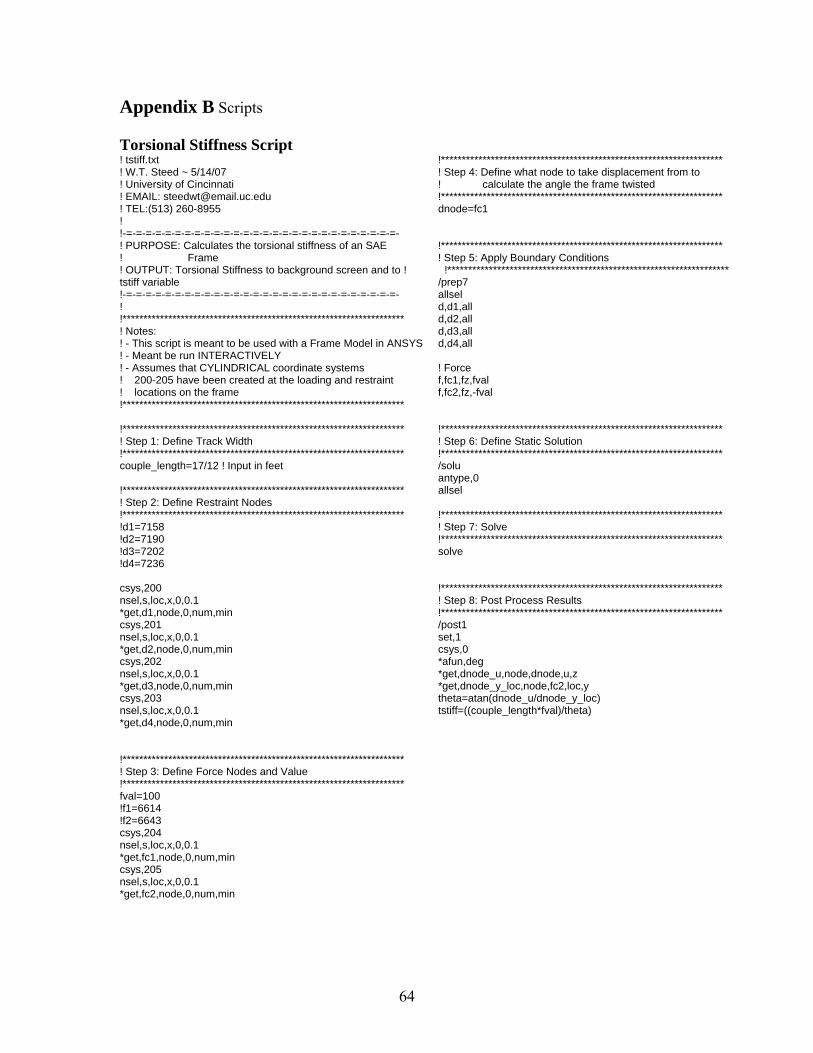
64
Appendix B Scripts Torsional Stiffness Script ! tstiff.txt ! W.T. Steed ~ 5/14/07 ! University of Cincinnati ! EMAIL: [email protected] ! TEL:(513) 260-8955 ! !-=-=-=-=-=-=-=-=-=-=-=-=-=-=-=-=-=-=-=-=-=-=-=-=-=-=-=-=- ! PURPOSE: Calculates the torsional stiffness of an SAE ! Frame ! OUTPUT: Torsional Stiffness to background screen and to ! tstiff variable !-=-=-=-=-=-=-=-=-=-=-=-=-=-=-=-=-=-=-=-=-=-=-=-=-=-=-=-=- ! !******************************************************************** ! Notes: ! - This script is meant to be used with a Frame Model in ANSYS ! - Meant be run INTERACTIVELY ! - Assumes that CYLINDRICAL coordinate systems ! 200-205 have been created at the loading and restraint ! locations on the frame !******************************************************************** !******************************************************************** ! Step 1: Define Track Width !******************************************************************** couple_length=17/12 ! Input in feet !******************************************************************** ! Step 2: Define Restraint Nodes !******************************************************************** !d1=7158 !d2=7190 !d3=7202 !d4=7236 csys,200 nsel,s,loc,x,0,0.1 *get,d1,node,0,num,min csys,201 nsel,s,loc,x,0,0.1 *get,d2,node,0,num,min csys,202 nsel,s,loc,x,0,0.1 *get,d3,node,0,num,min csys,203 nsel,s,loc,x,0,0.1 *get,d4,node,0,num,min !******************************************************************** ! Step 3: Define Force Nodes and Value !******************************************************************** fval=100 !f1=6614 !f2=6643 csys,204 nsel,s,loc,x,0,0.1 *get,fc1,node,0,num,min csys,205 nsel,s,loc,x,0,0.1 *get,fc2,node,0,num,min
!******************************************************************** ! Step 4: Define what node to take displacement from to ! calculate the angle the frame twisted !******************************************************************** dnode=fc1 !******************************************************************** ! Step 5: Apply Boundary Conditions
!******************************************************************** /prep7 allsel d,d1,all d,d2,all d,d3,all d,d4,all ! Force f,fc1,fz,fval f,fc2,fz,-fval !******************************************************************** ! Step 6: Define Static Solution !******************************************************************** /solu antype,0 allsel !******************************************************************** ! Step 7: Solve !******************************************************************** solve !******************************************************************** ! Step 8: Post Process Results !******************************************************************** /post1 set,1 csys,0 *afun,deg *get,dnode_u,node,dnode,u,z *get,dnode_y_loc,node,fc2,loc,y theta=atan(dnode_u/dnode_y_loc) tstiff=((couple_length*fval)/theta)
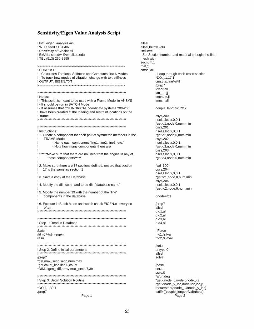
65
Sensitivity/Eigen Value Analysis Script ! tstif_eigen_analysis.ain ! W.T.Steed 11/20/06 ! University of Cincinnati ! EMAIL: [email protected] ! TEL:(513) 260-8955 !-=-=-=-=-=-=-=-=-=-=-=-=-=-=-=-=-=-=-=-=-=-=-=-=-=-=-=-=- ! PURPOSE: ! - Calculates Torsional Stiffness and Computes first 6 Modes ! - To track how modes of vibration change with tor. stiffness ! OUTPUT: EIGEN.TXT !-=-=-=-=-=-=-=-=-=-=-=-=-=-=-=-=-=-=-=-=-=-=-=-=-=-=-=-=- !******************************************************************** ! Notes: ! - This script is meant to be used with a Frame Model in ANSYS ! - It should be run in BATCH Mode ! - It assumes that CYLINDRICAL coordinate systems 200-205 ! have been created at the loading and restraint locations on the ! frame !******************************************************************** !******************************************************************** ! Instructions: ! 1. Create a component for each pair of symmetric members in the ! FRAME Model ! - Name each component "line1, line2, line3, etc." ! - Note how many components there are ! ! ******Make sure that there are no lines from the engine in any of ! these components***** ! ! 2. Make sure there are 17 sections defined, ensure that section ! 17 is the same as section 1 ! ! 3. Save a copy of the Database ! ! 4. Modify the /filn command to be /filn,"database name" ! ! 5. Modify the number 39 with the number of the "line" ! components in the database ! ! 6. Execute in Batch Mode and watch check EIGEN.txt every so ! often !******************************************************************** !******************************************************************** ! Step 1: Read in Database !******************************************************************** /batch /filn,07-tstiff-eigen resu !******************************************************************** ! Step 2: Define initial parameters !******************************************************************** /prep7 *get,max_secp,secp,num,max *get,count_line,line,0,count *DIM,eigen_stiff,array,max_secp,7,39 !******************************************************************** ! Step 3: Begin Solution Routine !******************************************************************** *DO,ii,1,39,1 /prep7
Page 1
allsel allsel,below,volu lsel,inve ! Set Section number and material to begin the first mesh with secnum,1 mat,1 cmsel,all ! Loop through each cross section *DO,jj,1,17,1 cmsel,s,line%ii% /prep7 lclear,all latt,,,,,,,jj secnum,jj lmesh,all couple_length=17/12 csys,200 nsel,s,loc,x,0,0.1 *get,d1,node,0,num,min csys,201 nsel,s,loc,x,0,0.1 *get,d2,node,0,num,min csys,202 nsel,s,loc,x,0,0.1 *get,d3,node,0,num,min csys,203 nsel,s,loc,x,0,0.1 *get,d4,node,0,num,min fval=100 csys,204 nsel,s,loc,x,0,0.1 *get,fc1,node,0,num,min csys,205 nsel,s,loc,x,0,0.1 *get,fc2,node,0,num,min dnode=fc1 /prep7 allsel d,d1,all d,d2,all d,d3,all d,d4,all ! Force f,fc1,fz,fval f,fc2,fz,-fval /solu antype,0 allsel solve /post1 set,1 csys,0 *afun,deg *get,dnode_u,node,dnode,u,z *get,dnode_y_loc,node,fc2,loc,y theta=atan(dnode_u/dnode_y_loc) tstiff=((couple_length*fval)/theta)
Page 2

66
! Store torsional stiffness in first column of eigen_stiff array eigen_stiff(jj,1,ii)=tstiff ! Clear Boundary Conditions /prep7 lsclear,all ! Start Modal Analysis /solu antype,modal MSAVE,0 MODOPT,LANB,12 EQSLV,SPAR MXPAND,0, , ,0 LUMPM,0 PSTRES,0 MODOPT,LANB,12,0,10000, ,OFF solve /solu ! Loop through Modes 7 to 12 and store in colums 2 ! through 7 of eigen_stiff *DO,kk,2,7,1 xx=kk+5 *get,freq,mode,xx,freq eigen_stiff(jj,kk,ii)=freq *ENDDO *ENDDO /prep7 ! Save all Parameters to eigen.txt PARSAV,ALL,'eigen','txt',' ' allsel *ENDDO
Page 3
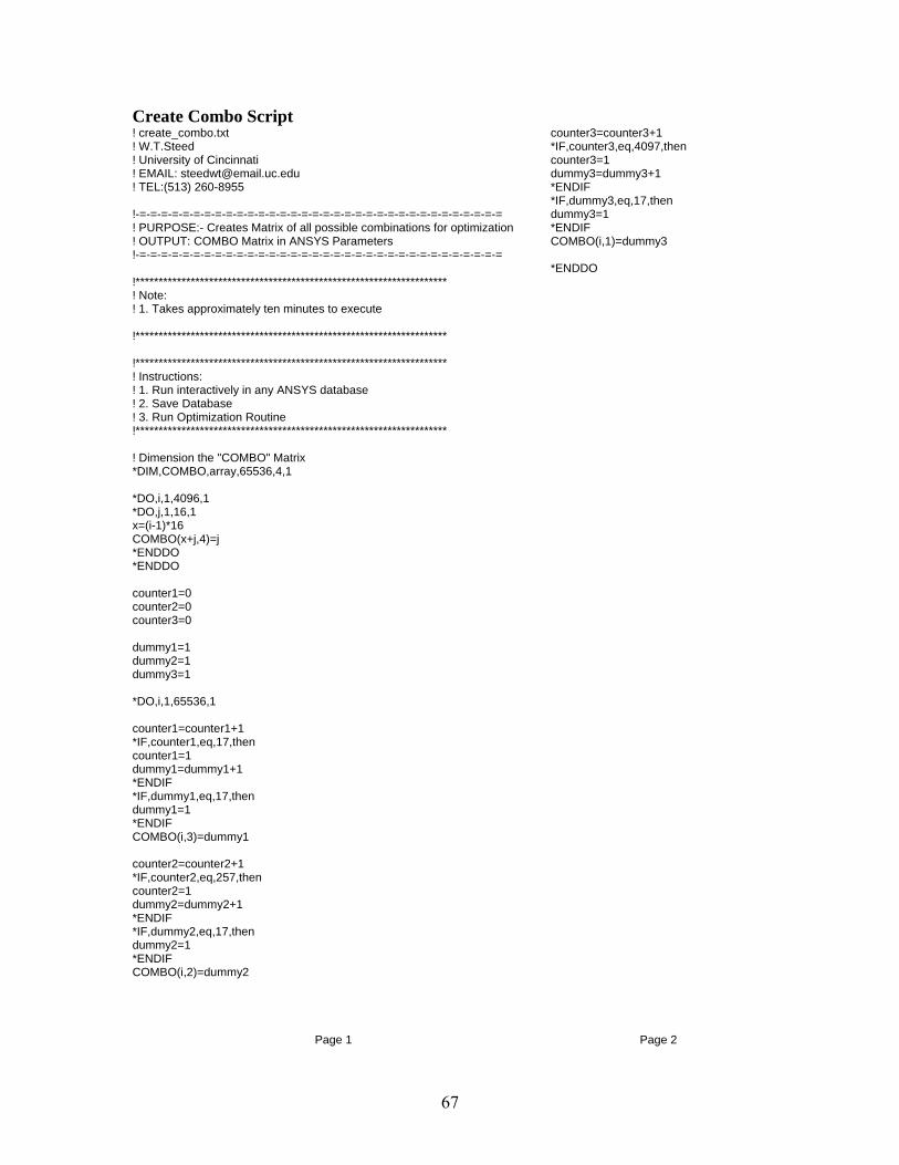
67
Create Combo Script ! create_combo.txt ! W.T.Steed ! University of Cincinnati ! EMAIL: [email protected] ! TEL:(513) 260-8955 !-=-=-=-=-=-=-=-=-=-=-=-=-=-=-=-=-=-=-=-=-=-=-=-=-=-=-=-=-=-=-=-=-=-= ! PURPOSE:- Creates Matrix of all possible combinations for optimization ! OUTPUT: COMBO Matrix in ANSYS Parameters !-=-=-=-=-=-=-=-=-=-=-=-=-=-=-=-=-=-=-=-=-=-=-=-=-=-=-=-=-=-=-=-=-=-= !******************************************************************** ! Note: ! 1. Takes approximately ten minutes to execute !******************************************************************** !******************************************************************** ! Instructions: ! 1. Run interactively in any ANSYS database ! 2. Save Database ! 3. Run Optimization Routine !******************************************************************** ! Dimension the "COMBO" Matrix *DIM,COMBO,array,65536,4,1 *DO,i,1,4096,1 *DO,j,1,16,1 x=(i-1)*16 COMBO(x+j,4)=j *ENDDO *ENDDO counter1=0 counter2=0 counter3=0 dummy1=1 dummy2=1 dummy3=1 *DO,i,1,65536,1 counter1=counter1+1 *IF,counter1,eq,17,then counter1=1 dummy1=dummy1+1 *ENDIF *IF,dummy1,eq,17,then dummy1=1 *ENDIF COMBO(i,3)=dummy1 counter2=counter2+1 *IF,counter2,eq,257,then counter2=1 dummy2=dummy2+1 *ENDIF *IF,dummy2,eq,17,then dummy2=1 *ENDIF COMBO(i,2)=dummy2
Page 1
counter3=counter3+1 *IF,counter3,eq,4097,then counter3=1 dummy3=dummy3+1 *ENDIF *IF,dummy3,eq,17,then dummy3=1 *ENDIF COMBO(i,1)=dummy3 *ENDDO
Page 2
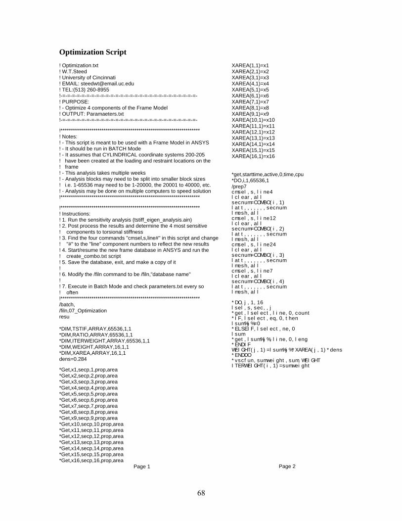
68
Optimization Script ! Optimization.txt ! W.T.Steed ! University of Cincinnati ! EMAIL: [email protected] ! TEL:(513) 260-8955 !-=-=-=-=-=-=-=-=-=-=-=-=-=-=-=-=-=-=-=-=-=-=-=-=-=-=-=-=- ! PURPOSE: ! - Optimize 4 components of the Frame Model ! OUTPUT: Paramaeters.txt !-=-=-=-=-=-=-=-=-=-=-=-=-=-=-=-=-=-=-=-=-=-=-=-=-=-=-=-=- !******************************************************************** ! Notes: ! - This script is meant to be used with a Frame Model in ANSYS ! - It should be run in BATCH Mode ! - It assumes that CYLINDRICAL coordinate systems 200-205 ! have been created at the loading and restraint locations on the ! frame ! - This analysis takes multiple weeks ! - Analysis blocks may need to be split into smaller block sizes ! i.e. 1-65536 may need to be 1-20000, the 20001 to 40000, etc. ! - Analysis may be done on multiple computers to speed solution !******************************************************************** !******************************************************************** ! Instructions: ! 1. Run the sensitivity analysis (tstiff_eigen_analysis.ain) ! 2. Post process the results and determine the 4 most sensitive ! components to torsional stiffness ! 3. Find the four commands "cmsel,s,line#" in this script and change ! "#" to the "line" component numbers to reflect the new results ! 4. Start/resume the new frame database in ANSYS and run the ! create_combo.txt script ! 5. Save the database, exit, and make a copy of it ! ! 6. Modify the /filn command to be /filn,"database name" ! ! 7. Execute in Batch Mode and check parameters.txt every so ! often !******************************************************************** /batch, /filn,07_Optimization resu *DIM,TSTIF,ARRAY,65536,1,1 *DIM,RATIO,ARRAY,65536,1,1 *DIM,ITERWEIGHT,ARRAY,65536,1,1 *DIM,WEIGHT,ARRAY,16,1,1 *DIM,XAREA,ARRAY,16,1,1 dens=0.284 *Get,x1,secp,1,prop,area *Get,x2,secp,2,prop,area *Get,x3,secp,3,prop,area *Get,x4,secp,4,prop,area *Get,x5,secp,5,prop,area *Get,x6,secp,6,prop,area *Get,x7,secp,7,prop,area *Get,x8,secp,8,prop,area *Get,x9,secp,9,prop,area *Get,x10,secp,10,prop,area *Get,x11,secp,11,prop,area *Get,x12,secp,12,prop,area *Get,x13,secp,13,prop,area *Get,x14,secp,14,prop,area *Get,x15,secp,15,prop,area *Get,x16,secp,16,prop,area
Page 1
XAREA(1,1)=x1 XAREA(2,1)=x2 XAREA(3,1)=x3 XAREA(4,1)=x4 XAREA(5,1)=x5 XAREA(6,1)=x6 XAREA(7,1)=x7 XAREA(8,1)=x8 XAREA(9,1)=x9 XAREA(10,1)=x10 XAREA(11,1)=x11 XAREA(12,1)=x12 XAREA(13,1)=x13 XAREA(14,1)=x14 XAREA(15,1)=x15 XAREA(16,1)=x16 *get,starttime,active,0,time,cpu *DO,i,1,65536,1 /prep7 cmsel,s,line4 lclear,all secnum=COMBO(i,1) latt,,,,,,,secnum lmesh,all cmsel,s,line12 lclear,all secnum=COMBO(i,2) latt,,,,,,,secnum lmesh,all cmsel,s,line24 lclear,all secnum=COMBO(i,3) latt,,,,,,,secnum lmesh,all cmsel,s,line7 lclear,all secnum=COMBO(i,4) latt,,,,,,,secnum lmesh,all *DO,j,1,16 lsel,s,sec,,j *get,lselect,line,0,count *IF,lselect,eq,0,then lsum%j%=0 *ELSEIF,lselect,ne,0 lsum *get,lsum%j%,line,0,leng *ENDIF WEIGHT(j,1)=lsum%j%*XAREA(j,1)*dens *ENDDO *vscfun,sumweight,sum,WEIGHT ITERWEIGHT(i,1)=sumweight
Page 2
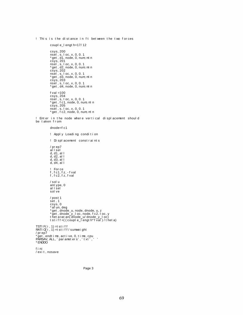
69
! This is the distance in ft between the two forces couple_length=17/12 csys,200 nsel,s,loc,x,0,0.1 *get,d1,node,0,num,min csys,201 nsel,s,loc,x,0,0.1 *get,d2,node,0,num,min csys,202 nsel,s,loc,x,0,0.1 *get,d3,node,0,num,min csys,203 nsel,s,loc,x,0,0.1 *get,d4,node,0,num,min fval=100 csys,204 nsel,s,loc,x,0,0.1 *get,fc1,node,0,num,min csys,205 nsel,s,loc,x,0,0.1 *get,fc2,node,0,num,min ! Enter in the node where vertical displacement should be taken from dnode=fc1 ! Apply Loading condition ! Displacement constraints /prep7 allsel d,d1,all d,d2,all d,d3,all d,d4,all ! Force f,fc1,fz,-fval f,fc2,fz,fval /solu antype,0 allsel solve /post1 set,1 csys,0 *afun,deg *get,dnode_u,node,dnode,u,z *get,dnode_y_loc,node,fc2,loc,y theta=atan(dnode_u/dnode_y_loc) tstiff=((couple_length*fval)/theta) TSTIF(i,1)=tstiff RATIO(i,1)=tstiff/sumweight /prep7 *get,endtime,active,0,time,cpu PARSAV,ALL,'parameters','txt',' ' *ENDDO fini /exit,nosave
Page 3
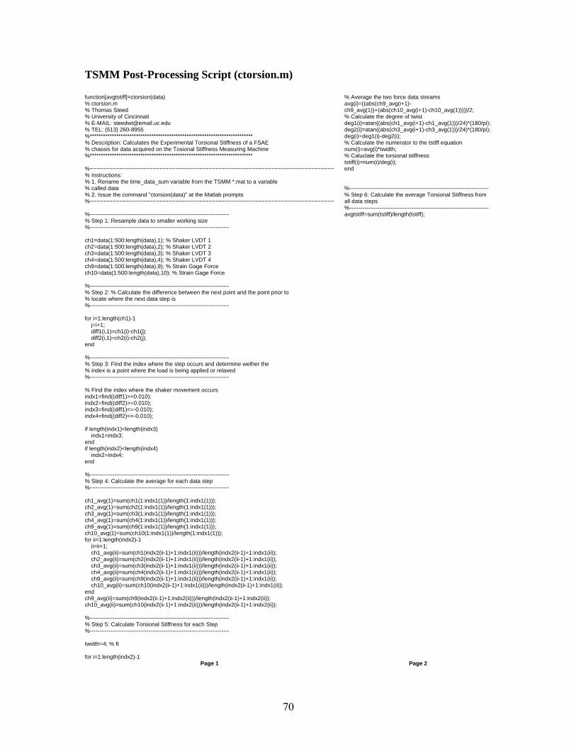
70
TSMM Post-Processing Script (ctorsion.m) function[avgtstiff]=ctorsion(data) % ctorsion.m % Thomas Steed % University of Cincinnati % E-MAIL: [email protected] % TEL: (513) 260-8955 %************************************************************************** % Description: Calculates the Experimental Torsional Stiffness of a FSAE % chassis for data acquired on the Tosional Stiffness Measuring Machine %************************************************************************** %~~~~~~~~~~~~~~~~~~~~~~~~~~~~~~~~~~~~~~~~~~~~~~~~~~~~~~~~~~~~~~~~~~~~~~~~~~ % Instructions: % 1. Rename the time_data_sum variable from the TSMM *.mat to a variable % called data % 2. Issue the command "ctorsion(data)" at the Matlab prompts %~~~~~~~~~~~~~~~~~~~~~~~~~~~~~~~~~~~~~~~~~~~~~~~~~~~~~~~~~~~~~~~~~~~~~~~~~~ %-------------------------------------------------------------------------- % Step 1: Resample data to smaller working size %-------------------------------------------------------------------------- ch1=data(1:500:length(data),1); % Shaker LVDT 1 ch2=data(1:500:length(data),2); % Shaker LVDT 2 ch3=data(1:500:length(data),3); % Shaker LVDT 3 ch4=data(1:500:length(data),4); % Shaker LVDT 4 ch9=data(1:500:length(data),9); % Strain Gage Force ch10=data(1:500:length(data),10); % Strain Gage Force %-------------------------------------------------------------------------- % Step 2: % Calculate the difference between the next point and the point prior to % locate where the next data step is %-------------------------------------------------------------------------- for i=1:length(ch1)-1 j=i+1; diff1(i,1)=ch1(i)-ch1(j); diff2(i,1)=ch2(i)-ch2(j); end %-------------------------------------------------------------------------- % Step 3: Find the index where the step occurs and determine wether the % index is a point where the load is being applied or relaxed %-------------------------------------------------------------------------- % Find the index where the shaker movement occurs indx1=find((diff1)>=0.010); indx2=find((diff2)>=0.010); indx3=find((diff1)<=-0.010); indx4=find((diff2)<=-0.010); if length(indx1)<length(indx3) indx1=indx3; end if length(indx2)<length(indx4) indx2=indx4; end %-------------------------------------------------------------------------- % Step 4: Calculate the average for each data step %-------------------------------------------------------------------------- ch1_avg(1)=sum(ch1(1:indx1(1))/length(1:indx1(1))); ch2_avg(1)=sum(ch2(1:indx1(1))/length(1:indx1(1))); ch3_avg(1)=sum(ch3(1:indx1(1))/length(1:indx1(1))); ch4_avg(1)=sum(ch4(1:indx1(1))/length(1:indx1(1))); ch9_avg(1)=sum(ch9(1:indx1(1))/length(1:indx1(1))); ch10_avg(1)=sum(ch10(1:indx1(1))/length(1:indx1(1))); for ii=1:length(indx2)-1 ii=ii+1; ch1_avg(ii)=sum(ch1(indx2(ii-1)+1:indx1(ii)))/length(indx2(ii-1)+1:indx1(ii)); ch2_avg(ii)=sum(ch2(indx2(ii-1)+1:indx1(ii)))/length(indx2(ii-1)+1:indx1(ii)); ch3_avg(ii)=sum(ch3(indx2(ii-1)+1:indx1(ii)))/length(indx2(ii-1)+1:indx1(ii)); ch4_avg(ii)=sum(ch4(indx2(ii-1)+1:indx1(ii)))/length(indx2(ii-1)+1:indx1(ii)); ch9_avg(ii)=sum(ch9(indx2(ii-1)+1:indx1(ii)))/length(indx2(ii-1)+1:indx1(ii)); ch10_avg(ii)=sum(ch10(indx2(ii-1)+1:indx1(ii)))/length(indx2(ii-1)+1:indx1(ii)); end ch9_avg(ii)=sum(ch9(indx2(ii-1)+1:indx2(ii)))/length(indx2(ii-1)+1:indx2(ii)); ch10_avg(ii)=sum(ch10(indx2(ii-1)+1:indx2(ii)))/length(indx2(ii-1)+1:indx2(ii)); %-------------------------------------------------------------------------- % Step 5: Calculate Torsional Stiffness for each Step %-------------------------------------------------------------------------- twidth=4; % ft for i=1:length(indx2)-1
Page 1
% Average the two force data streams avg(i)=((abs(ch9_avg(i+1)-ch9_avg(1))+(abs(ch10_avg(i+1)-ch10_avg(1)))))/2; % Calculate the degree of twist deg1(i)=atan((abs(ch1_avg(i+1)-ch1_avg(1)))/24)*(180/pi); deg2(i)=atan((abs(ch3_avg(i+1)-ch3_avg(1)))/24)*(180/pi); deg(i)=deg1(i)-deg2(i); % Calculate the numerator to the tstiff equation num(i)=avg(i)*twidth; % Caluclate the torsional stiffness tstiff(i)=num(i)/deg(i); end %-------------------------------------------------------------------------- % Step 6: Calculate the average Torsional Stiffness from all data steps %-------------------------------------------------------------------------- avgtstiff=sum(tstiff)/length(tstiff);
Page 2
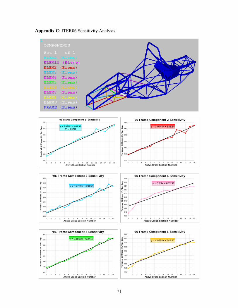
71
Appendix C: ITER06 Sensitivity Analysis
'06 Frame Component 1 Sensitivity
y = 0.6212x + 639.36R2 = 0.9743
638
640
642
644
646
648
650
1 2 3 4 5 6 7 8 9 10 11 12 13 14 15 16Ansys Cross Section Number
Tors
iona
l Sti
ffne
ss (
Ft.*
lb)/
Deg
.
'06 Frame Component 2 Sensitivity
y = 3.0444x + 635.54
630
640
650
660
670
680
690
1 2 3 4 5 6 7 8 9 10 11 12 13 14 15 16Ansys Cross Section Number
Tors
iona
l Sti
ffne
ss (
Ft.*
lb)/
Deg
.
'06 Frame Component 3 Sensitivity
y = 0.7753x + 638.56
638
640
642
644
646
648
650
652
654
1 2 3 4 5 6 7 8 9 10 11 12 13 14 15 16Ansys Cross Section Number
Tors
iona
l Sti
ffne
ss (
Ft.*
lb)/
Deg
.
'06 Frame Component 4 Sensitivity
y = 0.83x + 642.32
638
640
642
644
646
648
650
652
654
656
658
1 2 3 4 5 6 7 8 9 10 11 12 13 14 15 16Ansys Cross Section Number
Tors
iona
l Sti
ffne
ss (
Ft.*
lb)/
Deg
.
'06 Frame Component 5 Sensitivity
y = 0.1869x + 639.15
639
640
640
641
641
642
642
643
1 2 3 4 5 6 7 8 9 10 11 12 13 14 15 16Ansys Cross Section Number
Tors
iona
l Sti
ffne
ss (
Ft.*
lb)/
Deg
.
'06 Frame Component 6 Sensitivity
y = 4.0564x + 641.77
630
640
650
660
670
680
690
700
710
720
1 2 3 4 5 6 7 8 9 10 11 12 13 14 15 16Ansys Cross Section Number
Tors
iona
l Sti
ffne
ss (
Ft.*
lb)/
Deg
.
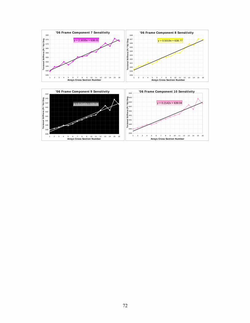
72
'06 Frame Component 7 Sensitivity
y = 2.3035x + 638.01
635
640
645
650
655
660
665
670
675
680
1 2 3 4 5 6 7 8 9 10 11 12 13 14 15 16Ansys Cross Section Number
Tors
iona
l Sti
ffne
ss (
Ft.*
lb)/
Deg
.
'06 Frame Component 8 Sensitivity
y = 0.5019x + 638.77
638
639
640
641
642
643
644
645
646
647
648
1 2 3 4 5 6 7 8 9 10 11 12 13 14 15 16Ansys Cross Section Number
Tors
iona
l Sti
ffne
ss (
Ft.*
lb)/
Deg
.
'06 Frame Component 9 Sensitivity
y = 0.2142x + 639.04
639
640
640
641
641
642
642
643
643
644
1 2 3 4 5 6 7 8 9 10 11 12 13 14 15 16Ansys Cross Section Number
Tors
iona
l Sti
ffne
ss (
Ft.*
lb)/
Deg
.
'06 Frame Component 10 Sensitivity
y = 0.2142x + 639.04
639
640
640
641
641
642
642
643
643
644
1 2 3 4 5 6 7 8 9 10 11 12 13 14 15 16
Ansys Cross Section Number
Tors
iona
l Sti
ffne
ss (
Ft.*
lb)/
Deg
.
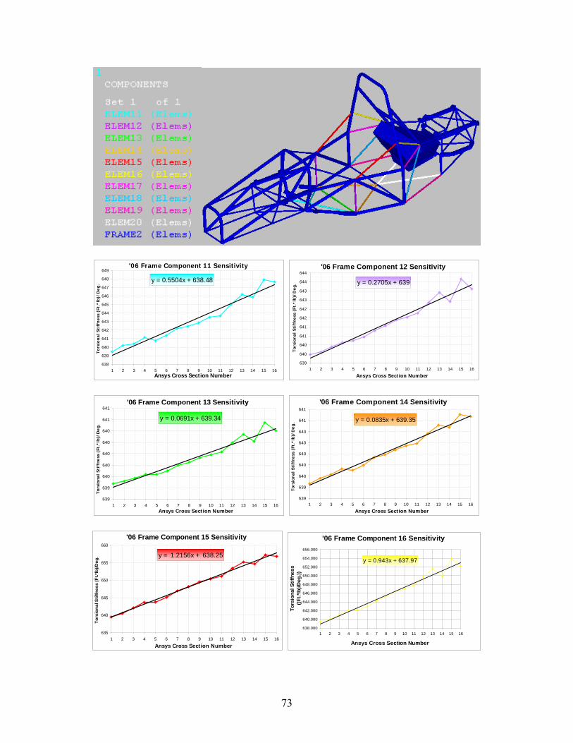
73
'06 Frame Component 11 Sensitivity
y = 0.5504x + 638.48
638
639
640
641
642
643
644
645
646
647
648
649
1 2 3 4 5 6 7 8 9 10 11 12 13 14 15 16Ansys Cross Section Number
Tors
iona
l Sti
ffne
ss (
Ft.*
lb)/
Deg
.
'06 Frame Component 12 Sensitivity
y = 0.2705x + 639
639
640
640
641
641
642
642
643
643
644
644
1 2 3 4 5 6 7 8 9 10 11 12 13 14 15 16
Ansys Cross Section Number
Tors
iona
l Sti
ffne
ss (
Ft.*
lb)/
Deg
.
'06 Frame Component 13 Sensitivity
y = 0.0691x + 639.34
639
639
640
640
640
640
640
641
641
1 2 3 4 5 6 7 8 9 10 11 12 13 14 15 16Ansys Cross Section Number
Tors
iona
l Sti
ffne
ss (
Ft.*
lb)/
Deg
.
'06 Frame Component 14 Sensitivity
y = 0.0835x + 639.35
639
639
640
640
640
640
640
641
641
1 2 3 4 5 6 7 8 9 10 11 12 13 14 15 16
Ansys Cross Section Number
Tors
iona
l Sti
ffne
ss (
Ft.*
lb)/
Deg
.
'06 Frame Component 15 Sensitivity
y = 1.2156x + 638.25
635
640
645
650
655
660
1 2 3 4 5 6 7 8 9 10 11 12 13 14 15 16
Ansys Cross Section Number
Tors
iona
l Stif
fnes
s (F
t.*lb
)/Deg
.
'06 Frame Component 16 Sensitivity
y = 0.943x + 637.97
638.000
640.000
642.000
644.000
646.000
648.000
650.000
652.000
654.000
656.000
1 2 3 4 5 6 7 8 9 10 11 12 13 14 15 16
Ansys Cross Section Number
Tors
iona
l Stif
fnes
s ((F
t.*lb
)/Deg
.))
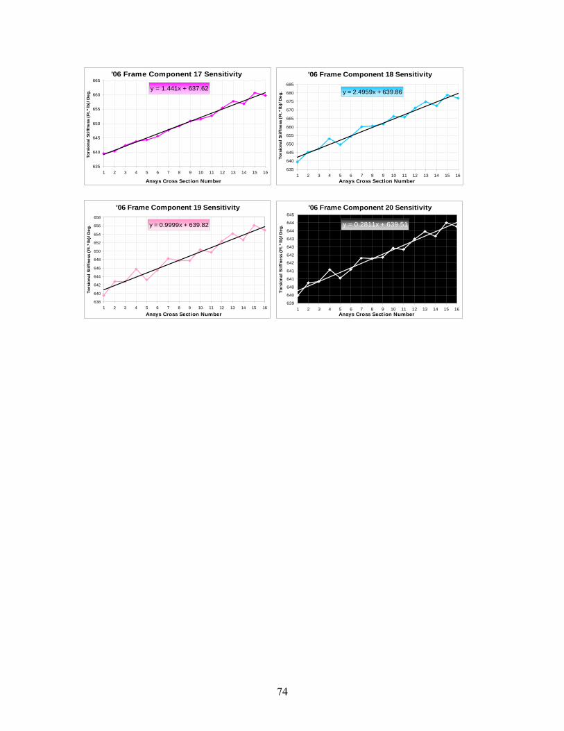
74
'06 Frame Component 17 Sensitivity
y = 1.441x + 637.62
635
640
645
650
655
660
665
1 2 3 4 5 6 7 8 9 10 11 12 13 14 15 16
Ansys Cross Section Number
Tors
iona
l Sti
ffne
ss (
Ft.*
lb)/
Deg
.
'06 Frame Component 18 Sensitivity
y = 2.4959x + 639.86
635
640
645
650
655
660
665
670
675
680
685
1 2 3 4 5 6 7 8 9 10 11 12 13 14 15 16Ansys Cross Section Number
Tors
iona
l Sti
ffne
ss (
Ft.*
lb)/
Deg
.
'06 Frame Component 19 Sensitivity
y = 0.9999x + 639.82
638
640
642
644
646
648
650
652
654
656
658
1 2 3 4 5 6 7 8 9 10 11 12 13 14 15 16
Ansys Cross Section Number
Tors
iona
l Sti
ffne
ss (
Ft.*
lb)/
Deg
.
'06 Frame Component 20 Sensitivity
y = 0.2811x + 639.51
639
640
640
641
641
642
642
643
643
644
644
645
1 2 3 4 5 6 7 8 9 10 11 12 13 14 15 16Ansys Cross Section Number
Tors
iona
l Sti
ffne
ss (
Ft.*
lb)/
Deg
.
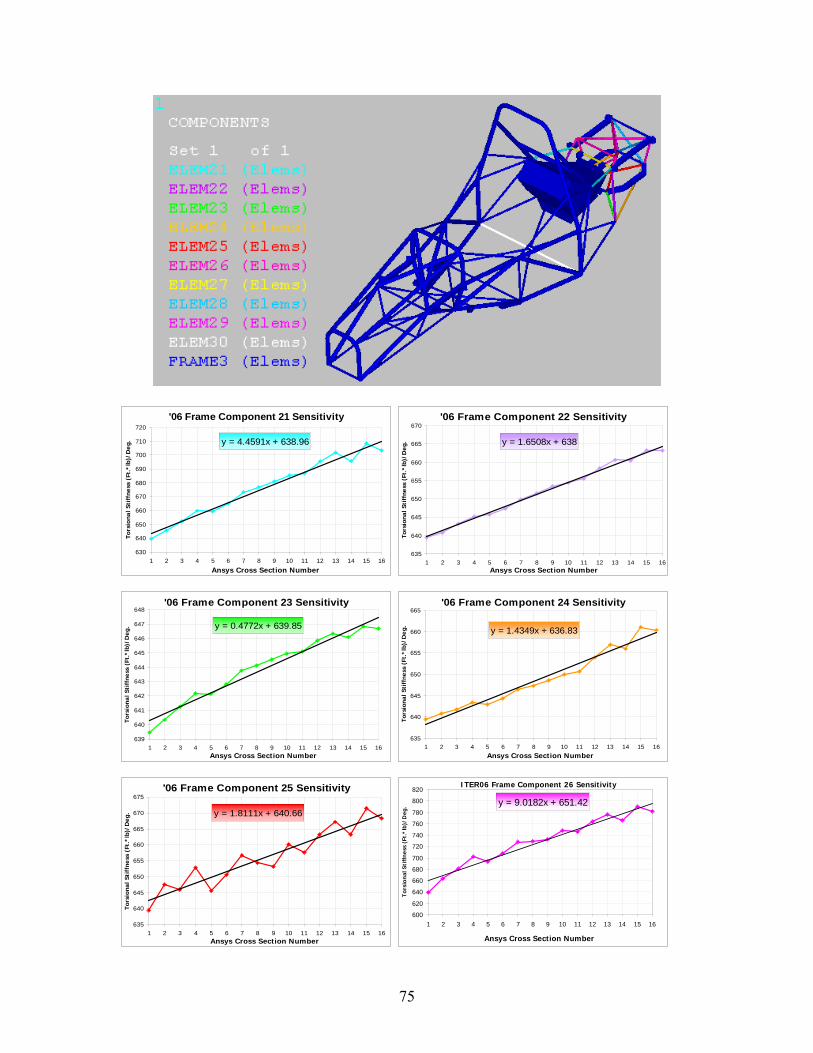
75
'06 Frame Component 21 Sensitivity
y = 4.4591x + 638.96
630
640
650
660
670
680
690
700
710
720
1 2 3 4 5 6 7 8 9 10 11 12 13 14 15 16Ansys Cross Section Number
Tors
iona
l Sti
ffne
ss (
Ft.*
lb)/
Deg
.
'06 Frame Component 22 Sensitivity
y = 1.6508x + 638
635
640
645
650
655
660
665
670
1 2 3 4 5 6 7 8 9 10 11 12 13 14 15 16Ansys Cross Section Number
Tors
iona
l Sti
ffne
ss (
Ft.*
lb)/
Deg
.
'06 Frame Component 23 Sensitivity
y = 0.4772x + 639.85
639
640
641
642
643
644
645
646
647
648
1 2 3 4 5 6 7 8 9 10 11 12 13 14 15 16Ansys Cross Section Number
Tors
iona
l Sti
ffne
ss (
Ft.*
lb)/
Deg
.
'06 Frame Component 24 Sensitivity
y = 1.4349x + 636.83
635
640
645
650
655
660
665
1 2 3 4 5 6 7 8 9 10 11 12 13 14 15 16Ansys Cross Section Number
Tors
iona
l Sti
ffne
ss (
Ft.*
lb)/
Deg
.
'06 Frame Component 25 Sensitivity
y = 1.8111x + 640.66
635
640
645
650
655
660
665
670
675
1 2 3 4 5 6 7 8 9 10 11 12 13 14 15 16Ansys Cross Section Number
Tors
iona
l Sti
ffne
ss (
Ft.*
lb)/
Deg
.
ITER06 Frame Component 26 Sensitivity
y = 9.0182x + 651.42
600
620
640
660
680
700
720
740
760
780
800
820
1 2 3 4 5 6 7 8 9 10 11 12 13 14 15 16
Ansys Cross Section Number
Tor
sion
al S
tiff
ness
(Ft
.*lb
)/D
eg.
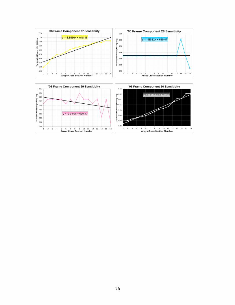
76
'06 Frame Component 27 Sensitivity
y = 3.8566x + 648.45
630
640
650
660
670
680
690
700
710
720
1 2 3 4 5 6 7 8 9 10 11 12 13 14 15 16Ansys Cross Section Number
Tors
iona
l Sti
ffne
ss (
Ft.*
lb)/
Deg
.
'06 Frame Component 28 Sensitivity
y = -5E-12x + 639.47
639
639
639
639
639
639
639
1 2 3 4 5 6 7 8 9 10 11 12 13 14 15 16Ansys Cross Section Number
Tors
iona
l Sti
ffne
ss (
Ft.*
lb)/
Deg
.
'06 Frame Component 29 Sensitivity
y = -3E-09x + 639.47
639
639
639
639
639
639
639
639
639
639
1 2 3 4 5 6 7 8 9 10 11 12 13 14 15 16Ansys Cross Section Number
Tors
iona
l Sti
ffne
ss (
Ft.*
lb)/
Deg
.
'06 Frame Component 30 Sensitivity
y = 0.1836x + 639.01
639
640
640
641
641
642
642
643
1 2 3 4 5 6 7 8 9 10 11 12 13 14 15 16Ansys Cross Section Number
Tors
iona
l Sti
ffne
ss (
Ft.*
lb)/
Deg
.
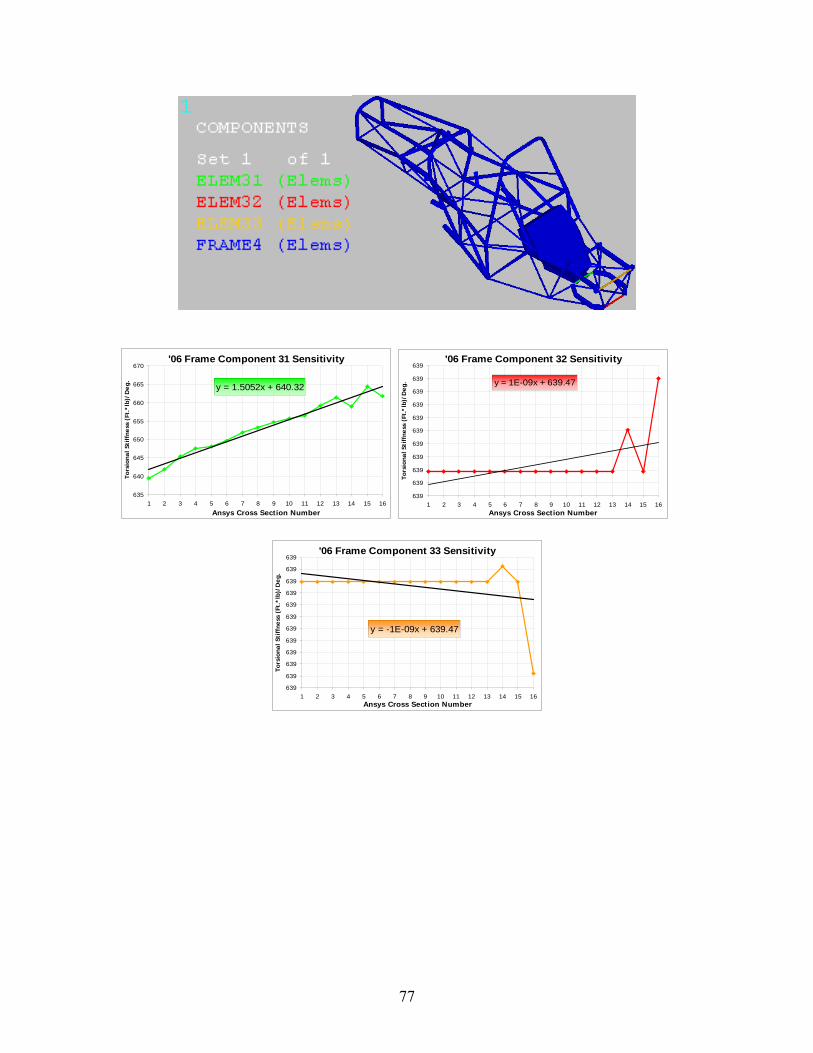
77
'06 Frame Component 31 Sensitivity
y = 1.5052x + 640.32
635
640
645
650
655
660
665
670
1 2 3 4 5 6 7 8 9 10 11 12 13 14 15 16Ansys Cross Section Number
Tors
iona
l Sti
ffne
ss (
Ft.*
lb)/
Deg
.
'06 Frame Component 32 Sensitivity
y = 1E-09x + 639.47
639
639
639
639
639
639
639
639
639
639
639
1 2 3 4 5 6 7 8 9 10 11 12 13 14 15 16Ansys Cross Section Number
Tors
iona
l Sti
ffne
ss (
Ft.*
lb)/
Deg
.
'06 Frame Component 33 Sensitivity
y = -1E-09x + 639.47
639
639
639
639
639
639
639
639
639
639
639
639
1 2 3 4 5 6 7 8 9 10 11 12 13 14 15 16Ansys Cross Section Number
Tors
iona
l Sti
ffne
ss (
Ft.*
lb)/
Deg
.
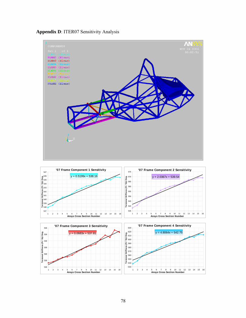
78
Appendix D: ITER07 Sensitivity Analysis
'07 Frame Component 1 Sensitivity
y = 0.5199x + 538.16
537
538
539
540
541
542
543
544
545
546
547
1 2 3 4 5 6 7 8 9 10 11 12 13 14 15 16Ansys Cross Section Number
Tors
iona
l Sti
ffne
ss (
Ft.*
lb)/
Deg
.
'07 Frame Component 2 Sensitivity
y = 2.0367x + 539.54
535
540
545
550
555
560
565
570
575
1 2 3 4 5 6 7 8 9 10 11 12 13 14 15 16Ansys Cross Section Number
Tors
iona
l Sti
ffne
ss (
Ft.*
lb)/
Deg
.
'07 Frame Component 3 Sensitivity
y = 0.0683x + 537.81
538
538
538
538
539
539
539
1 2 3 4 5 6 7 8 9 10 11 12 13 14 15 16Ansys Cross Section Number
Tors
iona
l Sti
ffne
ss (
Ft.*
lb)/
Deg
.
'07 Frame Component 4 Sensitivity
y = 4.8064x + 542.75
530
540
550
560
570
580
590
600
610
620
630
1 2 3 4 5 6 7 8 9 10 11 12 13 14 15 16Ansys Cross Section Number
Tors
iona
l Sti
ffne
ss (
Ft.*
lb)/
Deg
.
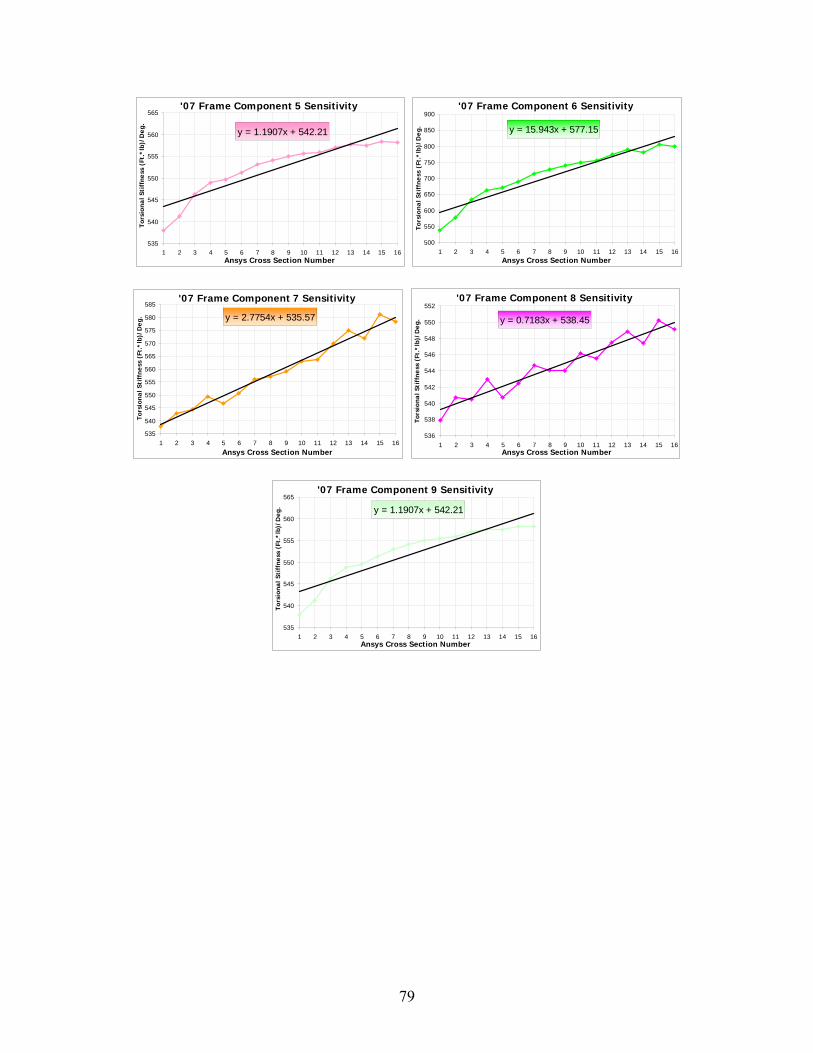
79
'07 Frame Component 5 Sensitivity
y = 1.1907x + 542.21
535
540
545
550
555
560
565
1 2 3 4 5 6 7 8 9 10 11 12 13 14 15 16Ansys Cross Section Number
Tors
iona
l Sti
ffne
ss (
Ft.*
lb)/
Deg
.
'07 Frame Component 6 Sensitivity
y = 15.943x + 577.15
500
550
600
650
700
750
800
850
900
1 2 3 4 5 6 7 8 9 10 11 12 13 14 15 16Ansys Cross Section Number
Tors
iona
l Sti
ffne
ss (
Ft.*
lb)/
Deg
.
'07 Frame Component 7 Sensitivity
y = 2.7754x + 535.57
535
540
545
550
555
560
565
570
575
580
585
1 2 3 4 5 6 7 8 9 10 11 12 13 14 15 16Ansys Cross Section Number
Tors
iona
l Sti
ffne
ss (
Ft.*
lb)/
Deg
.
'07 Frame Component 8 Sensitivity
y = 0.7183x + 538.45
536
538
540
542
544
546
548
550
552
1 2 3 4 5 6 7 8 9 10 11 12 13 14 15 16Ansys Cross Section Number
Tors
iona
l Sti
ffne
ss (
Ft.*
lb)/
Deg
.
'07 Frame Component 9 Sensitivity
y = 1.1907x + 542.21
535
540
545
550
555
560
565
1 2 3 4 5 6 7 8 9 10 11 12 13 14 15 16Ansys Cross Section Number
Tors
iona
l Sti
ffne
ss (
Ft.*
lb)/
Deg
.
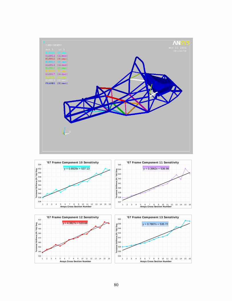
80
'07 Frame Component 10 Sensitivity
y = 0.8929x + 537.13
536
538
540
542
544
546
548
550
552
554
1 2 3 4 5 6 7 8 9 10 11 12 13 14 15 16Ansys Cross Section Number
Tors
iona
l Sti
ffne
ss (
Ft.*
lb)/
Deg
.
'07 Frame Component 11 Sensitivity
y = 0.3962x + 536.98
537
538
539
540
541
542
543
544
545
1 2 3 4 5 6 7 8 9 10 11 12 13 14 15 16Ansys Cross Section Number
Tors
iona
l Sti
ffne
ss (
Ft.*
lb)/
Deg
.
'07 Frame Component 12 Sensitivity
y = 4.3827x + 533.68
530
540
550
560
570
580
590
600
610
1 2 3 4 5 6 7 8 9 10 11 12 13 14 15 16
Ansys Cross Section Number
Tors
iona
l Sti
ffne
ss (
Ft.*
lb)/
Deg
.
'07 Frame Component 13 Sensitivity
y = 0.7807x + 535.72
534
536
538
540
542
544
546
548
550
1 2 3 4 5 6 7 8 9 10 11 12 13 14 15 16Ansys Cross Section Number
Tors
iona
l Sti
ffne
ss (
Ft.*
lb)/
Deg
.
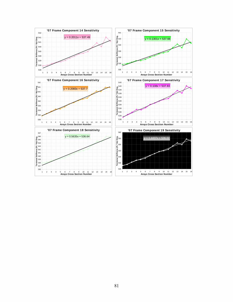
81
'07 Frame Component 14 Sensitivity
y = 0.2011x + 537.49
538
538
539
539
540
540
541
541
542
1 2 3 4 5 6 7 8 9 10 11 12 13 14 15 16Ansys Cross Section Number
Tors
iona
l Sti
ffne
ss (
Ft.*
lb)/
Deg
.
'07 Frame Component 15 Sensitivity
y = 0.1301x + 537.66
538
538
539
539
540
540
541
1 2 3 4 5 6 7 8 9 10 11 12 13 14 15 16Ansys Cross Section Number
Tors
iona
l Sti
ffne
ss (
Ft.*
lb)/
Deg
.
'07 Frame Component 16 Sensitivity
y = 0.2083x + 537.7
538
538
539
539
540
540
541
541
542
1 2 3 4 5 6 7 8 9 10 11 12 13 14 15 16Ansys Cross Section Number
Tors
iona
l Sti
ffne
ss (
Ft.*
lb)/
Deg
.
'07 Frame Component 17 Sensitivity
y = 0.108x + 537.83
538
538
538
538
539
539
539
539
539
540
540
1 2 3 4 5 6 7 8 9 10 11 12 13 14 15 16Ansys Cross Section Number
Tors
iona
l Sti
ffne
ss (
Ft.*
lb)/
Deg
.
'07 Frame Component 18 Sensitivity
y = 0.5635x + 536.64
536
537
538
539
540
541
542
543
544
545
546
547
1 2 3 4 5 6 7 8 9 10 11 12 13 14 15 16Ansys Cross Section Number
Tors
iona
l Sti
ffne
ss (
Ft.*
lb)/
Deg
.
'07 Frame Component 19 Sensitivity
y = 1.4437x + 536.02
535
540
545
550
555
560
565
1 2 3 4 5 6 7 8 9 10 11 12 13 14 15 16Ansys Cross Section Number
Tors
iona
l Sti
ffne
ss (
Ft.*
lb)/
Deg
.
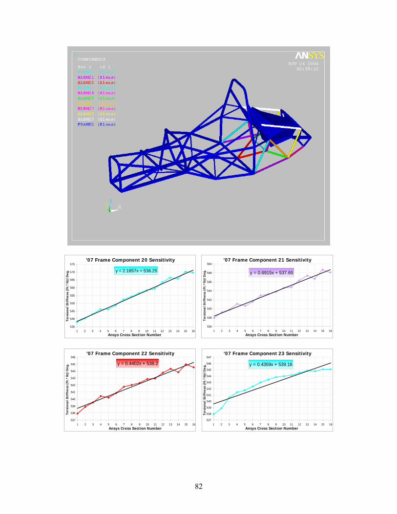
82
'07 Frame Component 20 Sensitivity
y = 2.1857x + 536.25
535
540
545
550
555
560
565
570
575
1 2 3 4 5 6 7 8 9 10 11 12 13 14 15 16Ansys Cross Section Number
Tors
iona
l Sti
ffne
ss (
Ft.*
lb)/
Deg
.
'07 Frame Component 21 Sensitivity
y = 0.6915x + 537.65
536
538
540
542
544
546
548
550
1 2 3 4 5 6 7 8 9 10 11 12 13 14 15 16Ansys Cross Section Number
Tors
iona
l Sti
ffne
ss (
Ft.*
lb)/
Deg
.
'07 Frame Component 22 Sensitivity
y = 0.4402x + 538.2
537
538
539
540
541
542
543
544
545
546
1 2 3 4 5 6 7 8 9 10 11 12 13 14 15 16Ansys Cross Section Number
Tors
iona
l Sti
ffne
ss (
Ft.*
lb)/
Deg
.
'07 Frame Component 23 Sensitivity
y = 0.4359x + 539.16
537
538
539
540
541
542
543
544
545
546
547
1 2 3 4 5 6 7 8 9 10 11 12 13 14 15 16Ansys Cross Section Number
Tors
iona
l Sti
ffne
ss (
Ft.*
lb)/
Deg
.
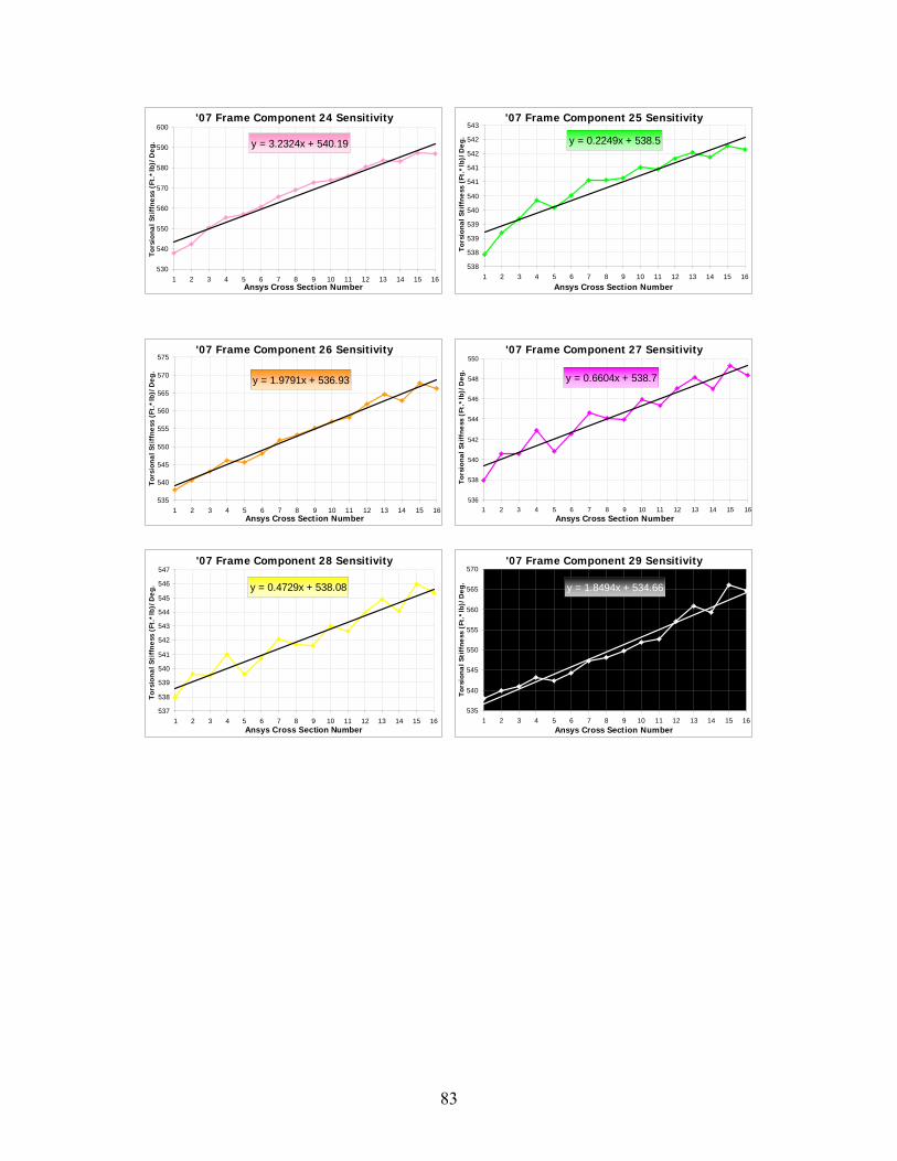
83
'07 Frame Component 24 Sensitivity
y = 3.2324x + 540.19
530
540
550
560
570
580
590
600
1 2 3 4 5 6 7 8 9 10 11 12 13 14 15 16Ansys Cross Section Number
Tors
iona
l Sti
ffne
ss (
Ft.*
lb)/
Deg
.
'07 Frame Component 25 Sensitivity
y = 0.2249x + 538.5
538
538
539
539
540
540
541
541
542
542
543
1 2 3 4 5 6 7 8 9 10 11 12 13 14 15 16Ansys Cross Section Number
Tors
iona
l Sti
ffne
ss (
Ft.*
lb)/
Deg
.
'07 Frame Component 26 Sensitivity
y = 1.9791x + 536.93
535
540
545
550
555
560
565
570
575
1 2 3 4 5 6 7 8 9 10 11 12 13 14 15 16Ansys Cross Section Number
Tors
iona
l Sti
ffne
ss (
Ft.*
lb)/
Deg
.
'07 Frame Component 27 Sensitivity
y = 0.6604x + 538.7
536
538
540
542
544
546
548
550
1 2 3 4 5 6 7 8 9 10 11 12 13 14 15 16Ansys Cross Section Number
Tors
iona
l Sti
ffne
ss (
Ft.*
lb)/
Deg
.
'07 Frame Component 28 Sensitivity
y = 0.4729x + 538.08
537
538
539
540
541
542
543
544
545
546
547
1 2 3 4 5 6 7 8 9 10 11 12 13 14 15 16Ansys Cross Section Number
Tors
iona
l Sti
ffne
ss (
Ft.*
lb)/
Deg
.
'07 Frame Component 29 Sensitivity
y = 1.8494x + 534.66
535
540
545
550
555
560
565
570
1 2 3 4 5 6 7 8 9 10 11 12 13 14 15 16Ansys Cross Section Number
Tors
iona
l Sti
ffne
ss (
Ft.*
lb)/
Deg
.
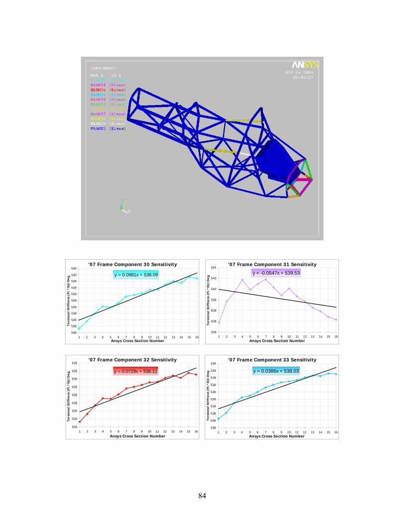
84
'07 Frame Component 30 Sensitivity
y = 0.0981x + 538.09
538
538
538
538
539
539
539
539
539
540
540
1 2 3 4 5 6 7 8 9 10 11 12 13 14 15 16Ansys Cross Section Number
Tors
iona
l Sti
ffne
ss (
Ft.*
lb)/
Deg
.
'07 Frame Component 31 Sensitivity
y = -0.0547x + 539.53
538
538
539
539
540
540
541
1 2 3 4 5 6 7 8 9 10 11 12 13 14 15 16Ansys Cross Section Number
Tors
iona
l Sti
ffne
ss (
Ft.*
lb)/
Deg
.
'07 Frame Component 32 Sensitivity
y = 0.0729x + 538.11
538
538
538
538
539
539
539
539
539
1 2 3 4 5 6 7 8 9 10 11 12 13 14 15 16Ansys Cross Section Number
Tors
iona
l Sti
ffne
ss (
Ft.*
lb)/
Deg
.
'07 Frame Component 33 Sensitivity
y = 0.0386x + 538.03
538
538
538
538
538
538
538
539
539
539
1 2 3 4 5 6 7 8 9 10 11 12 13 14 15 16Ansys Cross Section Number
Tors
iona
l Sti
ffne
ss (
Ft.*
lb)/
Deg
.
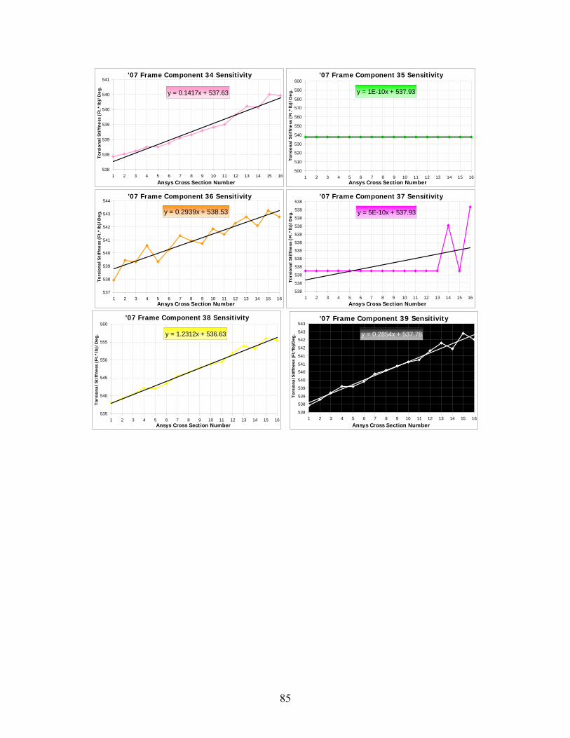
85
'07 Frame Component 34 Sensitivity
y = 0.1417x + 537.63
538
538
539
539
540
540
541
1 2 3 4 5 6 7 8 9 10 11 12 13 14 15 16Ansys Cross Section Number
Tors
iona
l Sti
ffne
ss (
Ft.*
lb)/
Deg
.
'07 Frame Component 35 Sensitivity
y = 1E-10x + 537.93
500
510
520
530
540
550
560
570
580
590
600
1 2 3 4 5 6 7 8 9 10 11 12 13 14 15 16Ansys Cross Section Number
Tors
iona
l Sti
ffne
ss (
Ft.*
lb)/
Deg
.
'07 Frame Component 36 Sensitivity
y = 0.2939x + 538.53
537
538
539
540
541
542
543
544
1 2 3 4 5 6 7 8 9 10 11 12 13 14 15 16Ansys Cross Section Number
Tors
iona
l Sti
ffne
ss (
Ft.*
lb)/
Deg
.
'07 Frame Component 37 Sensitivity
y = 5E-10x + 537.93
538
538
538
538
538
538
538
538
538
538
538
538
1 2 3 4 5 6 7 8 9 10 11 12 13 14 15 16Ansys Cross Section Number
Tors
iona
l Sti
ffne
ss (
Ft.*
lb)/
Deg
.
'07 Frame Component 38 Sensitivity
y = 1.2312x + 536.63
535
540
545
550
555
560
1 2 3 4 5 6 7 8 9 10 11 12 13 14 15 16Ansys Cross Section Number
Tors
iona
l Sti
ffne
ss (
Ft.*
lb)/
Deg
.
'07 Frame Component 39 Sensitivity
y = 0.2854x + 537.78
538
538
539
539
540
540
541
541
542
542
543
543
1 2 3 4 5 6 7 8 9 10 11 12 13 14 15 16
Ansys Cross Section Number
Tors
iona
l Stif
fnes
s (F
t.*lb
)/Deg
.
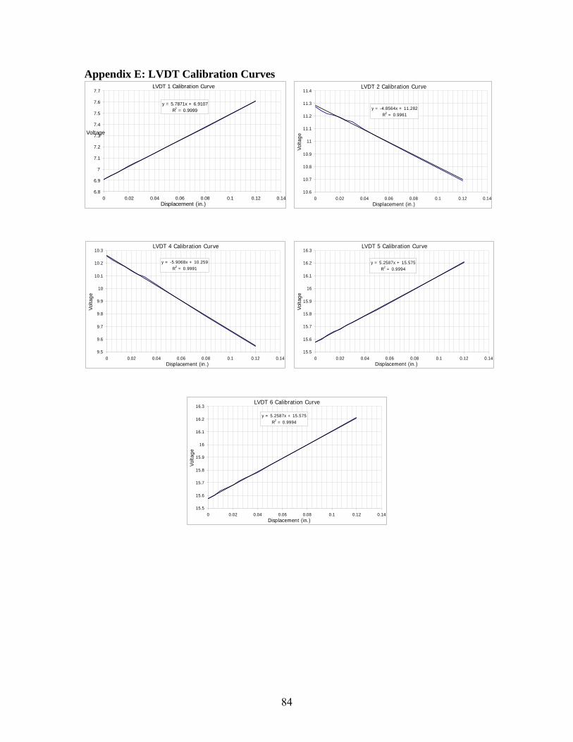
84
Appendix E: LVDT Calibration Curves
LVDT 2 Calibration Curve
y = -4.8564x + 11.282R2 = 0.9961
10.6
10.7
10.8
10.9
11
11.1
11.2
11.3
11.4
0 0.02 0.04 0.06 0.08 0.1 0.12 0.14Displacement (in.)
Volta
ge
LVDT 4 Calibration Curve
y = -5.9068x + 10.259R2 = 0.9991
9.5
9.6
9.7
9.8
9.9
10
10.1
10.2
10.3
0 0.02 0.04 0.06 0.08 0.1 0.12 0.14Displacement (in.)
Volta
ge
LVDT 5 Calibration Curve
y = 5.2587x + 15.575R2 = 0.9994
15.5
15.6
15.7
15.8
15.9
16
16.1
16.2
16.3
0 0.02 0.04 0.06 0.08 0.1 0.12 0.14Displacement (in.)
Volta
ge
LVDT 6 Calibration Curve
y = 5.2587x + 15.575R2 = 0.9994
15.5
15.6
15.7
15.8
15.9
16
16.1
16.2
16.3
0 0.02 0.04 0.06 0.08 0.1 0.12 0.14Displacement (in.)
Volta
ge
LVDT 1 Calibration Curve y = 5.7871x + 6.9107
R 2 = 0.9999
6.8
6.9
7 7.1
7.2
7.3
7.4
7.5
7.6
7.7
0 0.02 0.04 0.06 0.08 0.1 0.12 0.14Displacement (in.)
Voltage
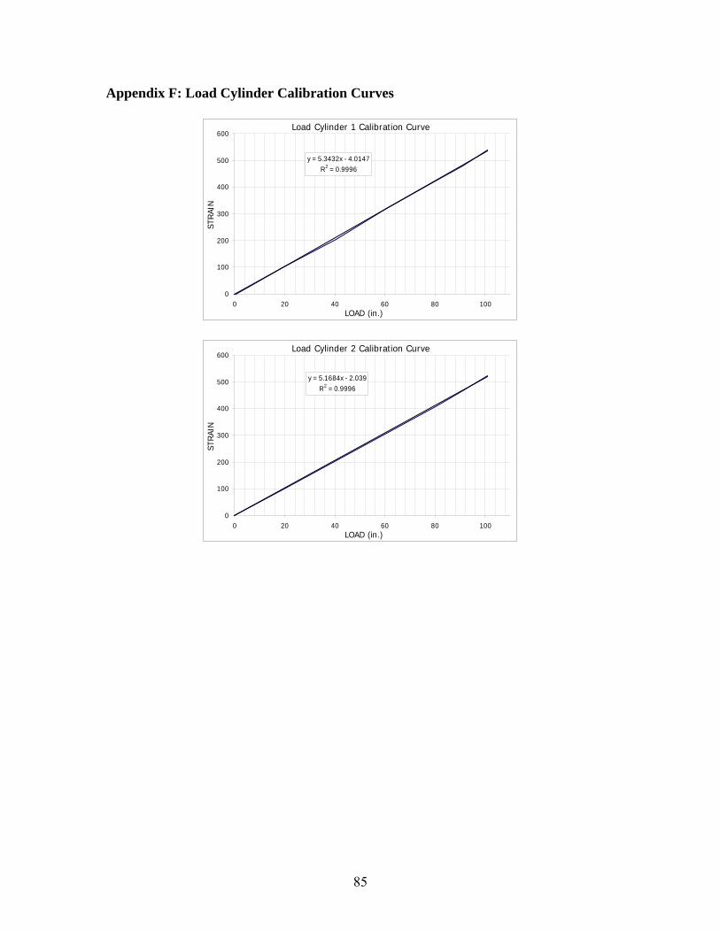
85
Appendix F: Load Cylinder Calibration Curves
Load Cylinder 1 Calibration Curve
y = 5.3432x - 4.0147R2 = 0.9996
0
100
200
300
400
500
600
0 20 40 60 80 100LOAD (in.)
STR
AIN
Load Cylinder 2 Calibration Curve
y = 5.1684x - 2.039R2 = 0.9996
0
100
200
300
400
500
600
0 20 40 60 80 100LOAD (in.)
STR
AIN
G.1
Appendix G: Torsional Stiffness Measuring Machine Assembly/Test Procedure
Torsional Stiffness Measuring Machine (TSMM) Assembly/Test Procedure
Author: Thomas Steed
G.2
Table of Contents 1. Test Information.......................................................................................................... 3 2. Testing Equipment List ............................................................................................... 3 3. TSMM Fixture Parts List ............................................................................................ 4 4. Pre-Test Notes ............................................................................................................. 6
4.1 “BUY OFFS” ............................................................................................................ 6 4.2 Bagging & Labeling .................................................................................................. 6 4.4 *****************************E-Stop******************************* 6
5. TSMM Assembly/Test Procedure.............................................................................. 7 6. Appendix A: Sensor Record Sheet ........................................................................... 21 7. Appendix B: TSMM Test Data Record Tables......................................................... 22 8. Appendix C: Equipment Record .............................................................................. 23 9. Appendix D: Channel Record ................................................................................... 23
Table of Figures Figure 1: TSMM Fixture Exploded View ........................................................................... 5 Figure 2: 4 Post Shaker Software Startup ........................................................................... 7 Figure 3: Vishay Amp. Banana Clip Plug-ins .................................................................... 8 Figure 4: 4 Post Height Software Commands................................................................... 10 Figure 5: Vishay Amp. Banana Clip Plug-ins .................................................................. 14 Figure 6: DYMAC Power Supply Terminals ................................................................... 15 Figure 7: TSMM Sensor Locations................................................................................... 21
Table of Tables Table 1: Testing Equipment List ......................................................................................... 3 Table 2: TSMM Fixture Parts List ...................................................................................... 4 Table 3: Strain Gage Wiring Scheme ................................................................................. 8 Table 4: Ride Height Shock Lengths ................................................................................ 10 Table 5: Strain Gage Wiring Scheme ............................................................................... 14 Table 6: Transducer Log ................................................................................................... 21 Table 7: TSMM Test 1 0.020" Increment ......................................................................... 22 Table 8: TSMM Test 2 0.050" Increment ......................................................................... 22 Table 9: Equipment Record .............................................................................................. 23 Table 10: Channel Record ................................................................................................ 23
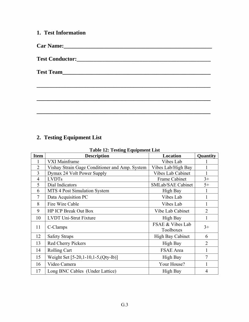
G.3
1. Test Information Car Name:____________________________________________________
Test Conductor:_______________________________________________
Test Team____________________________________________________
_____________________________________________________________
_____________________________________________________________
_____________________________________________________________
2. Testing Equipment List
Table 12: Testing Equipment List Item Description Location Quantity
1 VXI Mainframe Vibes Lab 1 2 Vishay Strain Gage Conditioner and Amp. System Vibes Lab/High Bay 1 3 Dymax 24 Volt Power Supply Vibes Lab Cabinet 1 4 LVDTs Frame Cabinet 3+ 5 Dial Indicators SMLab/SAE Cabinet 5+ 6 MTS 4 Post Simulation System High Bay 1 7 Data Acquisition PC Vibes Lab 1 8 Fire Wire Cable Vibes Lab 1 9 HP ICP Break Out Box Vibe Lab Cabinet 2 10 LVDT Uni-Strut Fixture High Bay 1
11 C-Clamps FSAE & Vibes Lab Toolboxes 3+
12 Safety Straps High Bay Cabinet 6 13 Red Cherry Pickers High Bay 2 14 Rolling Cart FSAE Area 1 15 Weight Set [5-20,1-10,1-5,(Qty-lb)] High Bay 7 16 Video Camera Your House? 1 17 Long BNC Cables (Under Lattice) High Bay 4
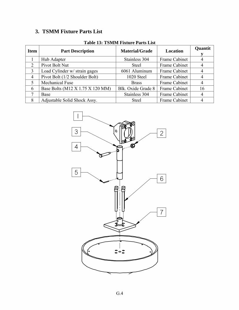
G.4
3. TSMM Fixture Parts List
Table 13: TSMM Fixture Parts List
Item Part Description Material/Grade Location Quantity
1 Hub Adapter Stainless 304 Frame Cabinet 4 2 Pivot Bolt Nut Steel Frame Cabinet 4 3 Load Cylinder w/ strain gages 6061 Aluminum Frame Cabinet 4 4 Pivot Bolt (1/2 Shoulder Bolt) 1020 Steel Frame Cabinet 4 5 Mechanical Fuse Brass Frame Cabinet 4 6 Base Bolts (M12 X 1.75 X 120 MM) Blk. Oxide Grade 8 Frame Cabinet 16 7 Base Stainless 304 Frame Cabinet 4 8 Adjustable Solid Shock Assy. Steel Frame Cabinet 4
1
23
4
56
7

G.5
Figure 56: TSMM Fixture Exploded View
G.6
4. Pre-Test Notes In preparation for testing, organizing equipment and hardware will save time and frustration. It is recommended that the equipment list and procedure are thoroughly read over. Depending upon the extravagance of the suspension some major modifications to the adjustable solid shocks and alignment spacers may be required. Consulting the current suspension team leader for the length and the proper spacer thickness is strongly suggested when using the solid shocks. Any miscommunication between the test conductor and the suspension and/or frame team leader could potentially be very hazardous to the car. Having this person on hand at the time of the test is suggested. However, with the knowledge in this procedure and use of the step by step instructions will create an environment that is safe for all team members and the car. 4.1 “BUY OFFS” This procedure has been written in a manner in which each step is intended to be bought off by the test conductor. It is EXTREMELY important that each step is read and executed as written. If at any time a step is read and not understood testing should halt and a group consensus should be met before proceeding. This is not a test that should be conducted at a time where personnel is fatigued. Each step MUST be bought off for completion to protect the hardware, NO MATTER how juvenile or tedious it might be. Buying off shall be completed by any member in the testing team. “Buy offs” shall be completed by initialing and dating the “Buy off” cell in each step of the procedure. The team member who “Buys Off” takes the responsibility that the step has been completed. 4.2 Bagging & Labeling Throughout the testing process hardware should be bagged and labeled accordingly. Bagging and labeling all the removed parts will prevent any problems remembering the hardware configuration during re-installation. Having extra hardware after re-installing all the parts is not acceptable. Tires should be labeled RF, LF, RR, or LR before they are removed from the car. Each shock should be bagged and labeled with RF, LF, RR, or LR and an orientation arrow to ensure proper re-installation. 4.3 Testing Duration Following this procedure should limit the test duration to no more than 6 hours. However, assuming that Murphy’s Law is always in effect, expect to dedicate a full day to testing. It is absolutely necessary to remove the car from the TSMM fixture at the end of the day. With that said, do not start testing in the late afternoon. 4.4 *****************************E-Stop******************************* The MTS 4 Post Simulation System is equipped with two E-Stop buttons. These buttons are an EXTREME Hazard to the car. If at any time the car is connected to the fixture with solid shocks installed these buttons MUST NOT be tripped. The E-Stop buttons when depressed will cause each post to return to a natural zero based on the hydraulic pressure in the system. These positions are reached very quickly and at different rates. If an E-Stop is tripped there will be damage to the chassis. All members of the test team must be made aware of this.
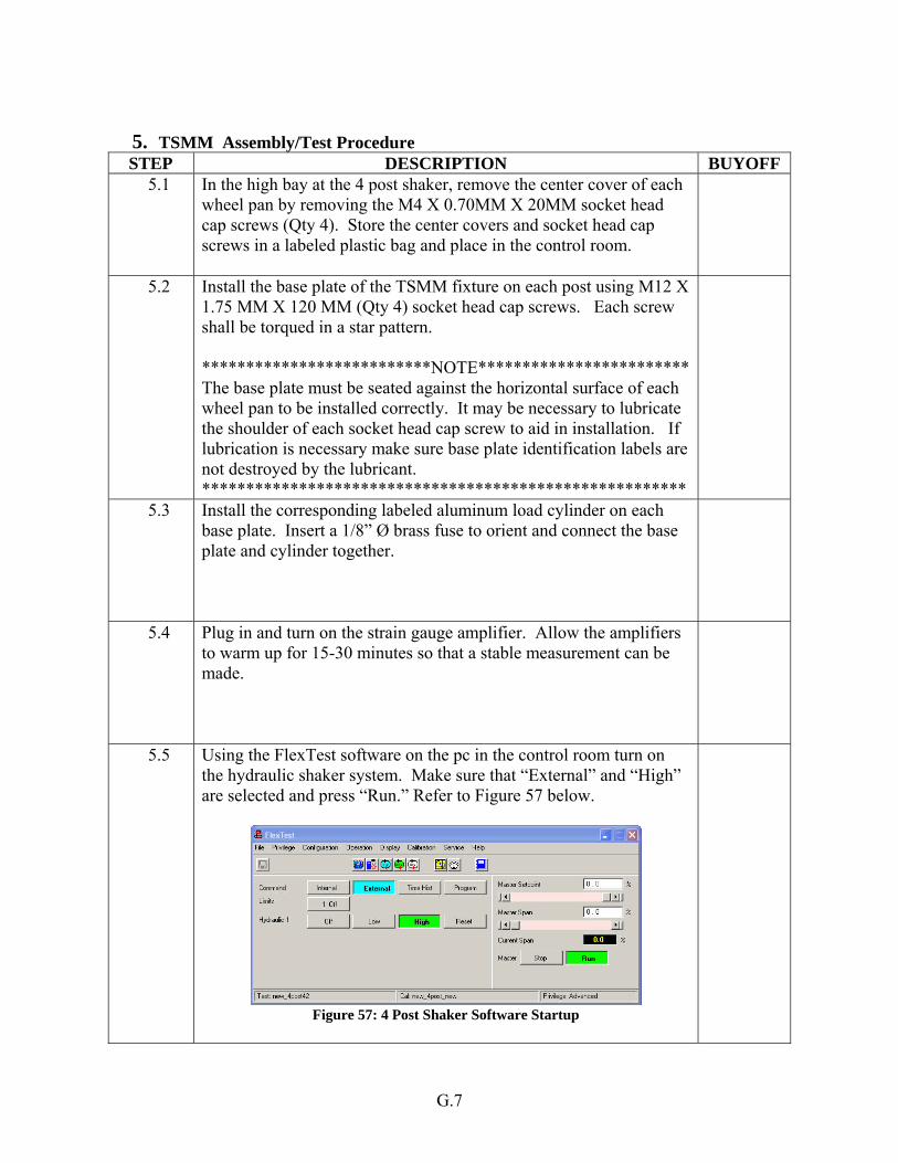
G.7
5. TSMM Assembly/Test Procedure STEP DESCRIPTION BUYOFF
5.1 In the high bay at the 4 post shaker, remove the center cover of each wheel pan by removing the M4 X 0.70MM X 20MM socket head cap screws (Qty 4). Store the center covers and socket head cap screws in a labeled plastic bag and place in the control room.
5.2 Install the base plate of the TSMM fixture on each post using M12 X 1.75 MM X 120 MM (Qty 4) socket head cap screws. Each screw shall be torqued in a star pattern. **************************NOTE************************ The base plate must be seated against the horizontal surface of each wheel pan to be installed correctly. It may be necessary to lubricate the shoulder of each socket head cap screw to aid in installation. If lubrication is necessary make sure base plate identification labels are not destroyed by the lubricant. *******************************************************
5.3 Install the corresponding labeled aluminum load cylinder on each base plate. Insert a 1/8” Ø brass fuse to orient and connect the base plate and cylinder together.
5.4 Plug in and turn on the strain gauge amplifier. Allow the amplifiers to warm up for 15-30 minutes so that a stable measurement can be made.
5.5 Using the FlexTest software on the pc in the control room turn on the hydraulic shaker system. Make sure that “External” and “High” are selected and press “Run.” Refer to Figure 57 below.
Figure 57: 4 Post Shaker Software Startup
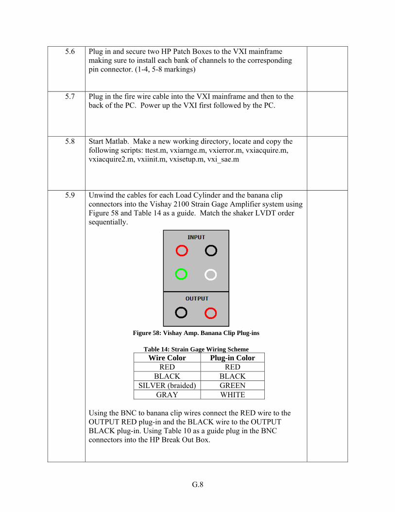
G.8
5.6 Plug in and secure two HP Patch Boxes to the VXI mainframe making sure to install each bank of channels to the corresponding pin connector. (1-4, 5-8 markings)
5.7 Plug in the fire wire cable into the VXI mainframe and then to the back of the PC. Power up the VXI first followed by the PC.
5.8 Start Matlab. Make a new working directory, locate and copy the following scripts: ttest.m, vxiarnge.m, vxierror.m, vxiacquire.m, vxiacquire2.m, vxiinit.m, vxisetup.m, vxi_sae.m
5.9 Unwind the cables for each Load Cylinder and the banana clip connectors into the Vishay 2100 Strain Gage Amplifier system using Figure 58 and Table 14 as a guide. Match the shaker LVDT order sequentially.
Figure 58: Vishay Amp. Banana Clip Plug-ins
Table 14: Strain Gage Wiring Scheme
Wire Color Plug-in Color RED RED
BLACK BLACK SILVER (braided) GREEN
GRAY WHITE Using the BNC to banana clip wires connect the RED wire to the OUTPUT RED plug-in and the BLACK wire to the OUTPUT BLACK plug-in. Using Table 10 as a guide plug in the BNC connectors into the HP Break Out Box.
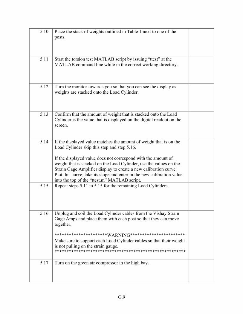
G.9
5.10 Place the stack of weights outlined in Table 1 next to one of the posts.
5.11 Start the torsion test MATLAB script by issuing “ttest” at the MATLAB command line while in the correct working directory.
5.12 Turn the monitor towards you so that you can see the display as weights are stacked onto the Load Cylinder.
5.13 Confirm that the amount of weight that is stacked onto the Load Cylinder is the value that is displayed on the digital readout on the screen.
5.14 If the displayed value matches the amount of weight that is on the Load Cylinder skip this step and step 5.16. If the displayed value does not correspond with the amount of weight that is stacked on the Load Cylinder, use the values on the Strain Gage Amplifier display to create a new calibration curve. Plot this curve, take its slope and enter in the new calibration value into the top of the “ttest.m” MATLAB script.
5.15 Repeat steps 5.11 to 5.15 for the remaining Load Cylinders.
5.16 Unplug and coil the Load Cylinder cables from the Vishay Strain Gage Amps and place them with each post so that they can move together. **********************WARNING*********************** Make sure to support each Load Cylinder cables so that their weight is not pulling on the strain gauge. *******************************************************
5.17 Turn on the green air compressor in the high bay.
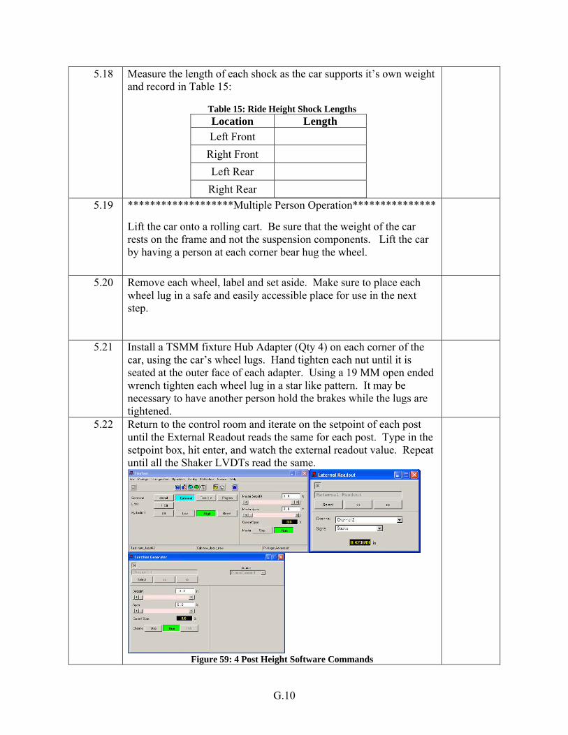
G.10
5.18 Measure the length of each shock as the car supports it’s own weight and record in Table 15:
Table 15: Ride Height Shock Lengths Location Length Left Front
Right Front Left Rear
Right Rear
5.19 *******************Multiple Person Operation*************** Lift the car onto a rolling cart. Be sure that the weight of the car rests on the frame and not the suspension components. Lift the car by having a person at each corner bear hug the wheel.
5.20 Remove each wheel, label and set aside. Make sure to place each wheel lug in a safe and easily accessible place for use in the next step.
5.21 Install a TSMM fixture Hub Adapter (Qty 4) on each corner of the car, using the car’s wheel lugs. Hand tighten each nut until it is seated at the outer face of each adapter. Using a 19 MM open ended wrench tighten each wheel lug in a star like pattern. It may be necessary to have another person hold the brakes while the lugs are tightened.
5.22 Return to the control room and iterate on the setpoint of each post until the External Readout reads the same for each post. Type in the setpoint box, hit enter, and watch the external readout value. Repeat until all the Shaker LVDTs read the same.
Figure 59: 4 Post Height Software Commands

G.11
5.23 Consult the current suspension team leader if doubtful of measurement accuracy of Table 15. Adjust the length of the solid shocks to match that of Table 15 and label accordingly.
5.24 *******************Two Person Operation****************** While supporting the suspension at the hub, remove the shock/damper by backing out the ¼” – 28 bolts at the bell-crank and frame mount. Make sure to carefully watch for any loose spacers. Bag, label and store shock and any necessary hardware.
5.25 Install solid shock with alignment spacers using ¼”-28 bolts. Properly torque each bolt.
5.26 Repeat steps 5.25 and 5.26 for each corner of the car.
5.27 Raise the blue lift in the high bay all the way up and rotate the support arms away from the 4 Post Shaker area.
5.28 Roll the cart/car into the middle of the 4 Post Shaker area so that the front point towards SMLAB.
5.29 Place a cherry picker at the front of the car. Install a strap on the cherry picker’s hook/clip and raise it so that the boom will not hit the car. Position the cherry picker so that the strap wraps around the front end and supports the bottom frame rails.
5.30 Roll the second cherry picker to the rear of the car. Install a strap on the clip and raise the boom. Position the cherry picker so that the strap will wrap around the jack bar.
5.31 With another person raise each cherry picker together so that the car will clear each post.

G.12
5.32 Lower the blue lift a small amount and as a safety measure wrap a strap around the bottom side impact tube of the frame and up to each arm. Provide each strap with ample slack so that when the frame is attached to the fixture it will not be supported.
5.33 Return to the control room and check that the external readout of each post’s LVDT still reads as it did before. If it has made any significant change more time is needed for the fluid to reach a constant operating temperature. Wait 10 minutes if LVDTs are still fluctuating.
5.34 Make any adjustments to the height of the rear of the car so that the hub adapter and load cylinder pivot points match.
5.35 **********************WARNING*********************** Steps 5.36 through 5.47 must be completed in the sequence described. If not the potential of pre-loading the suspension/frame is greatly increased. *******************************************************
5.36 Install the air supply at the right rear post and turn on. Gently float the post into a planar position so that the car can be translated with the cherry picker so that the slot of the Hub Adapter can slide around the Load Cylinder. Turn off the air supply!
5.37 Make any vertical adjustments by raising/lowering the cherry picker so that the pivot holes match in each part. Install the pivot bolt and hand tighten the nut. *************************NOTE************************* A hammer may be necessary to TAP the pivot bolt in. *******************************************************
5.38 Remove the air supply to the right rear post and install on the left rear post. Turn the air supply on.
5.39 Wrestle the left rear post so that it is floating and can be easily moved with a small amount of force. Make sure that the post is floating and not oscillating because of low air pressure! Very gently float the post so that the Load Cylinder is in the slot of the Hub Adapter. Turn off the air supply!

G.13
5.40 Make any out of plane adjustments by raising/lowering the cherry picker so that the pivot holes match in each part. Install the pivot bolt and hand tighten the nut. **************************NOTE************************ The air supply may be turned on to make small adjustments if necessary. *******************************************************
5.41 Adjust the height of the front of the car by raising/lowering the boom of the cherry picker. Position the height so that the pivot point of the Load cylinder matches with the Hub Adapter.
5.42 Remove the air supply and install on the front left post. If necessary wait for air pressure to return before turning on.
5.43 Wrestle the left front post so that it is floating and can be easily moved with a small amount of force. Make sure that the post is floating and not oscillating because of low air pressure! Very gently float the post so that the Load Cylinder is in the slot of the Hub Adapter. Turn off the air supply!
5.44 Make any out of plane adjustments by raising/lowering the cherry picker so that the pivot holes match in each part. Install the pivot bolt and hand tighten the nut. **************************Note************************* The air supply may be turned on to make small adjustments if necessary. *******************************************************
5.45 Remove the air supply from the left front post and install on the right front post. Wait until air pressure has been completely been restored.
5.46 Wrestle the right front post so that it is floating and can be easily moved with a small amount of force. Make sure that the post is floating and not oscillating because of low air pressure! Very gently float the post so that the Load Cylinder is in the slot of the Hub Adapter. Turn off the air supply!
5.47 Make any out of plane adjustments by raising/lowering the cherry picker so that the pivot holes match in each part. Install the pivot bolt and hand tighten the nut. **************************Note************************* The air supply may be turned on to make small adjustments if necessary. *******************************************************
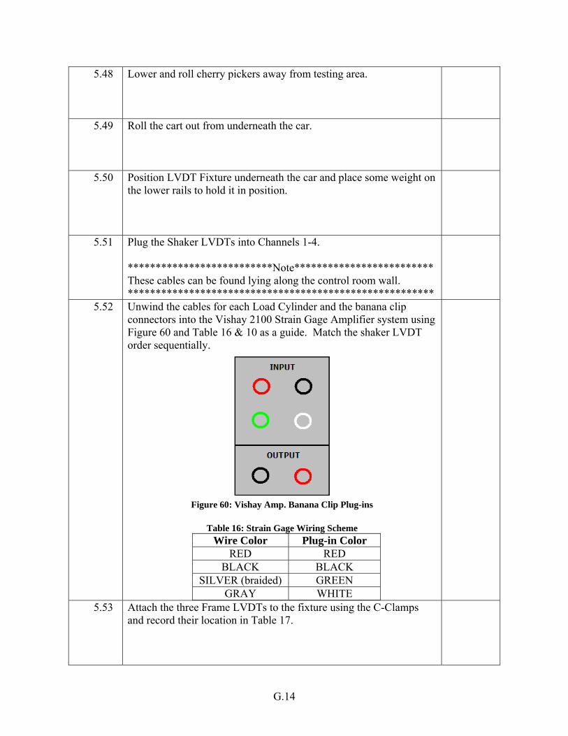
G.14
5.48 Lower and roll cherry pickers away from testing area.
5.49 Roll the cart out from underneath the car.
5.50 Position LVDT Fixture underneath the car and place some weight on the lower rails to hold it in position.
5.51 Plug the Shaker LVDTs into Channels 1-4. **************************Note************************* These cables can be found lying along the control room wall. *******************************************************
5.52 Unwind the cables for each Load Cylinder and the banana clip connectors into the Vishay 2100 Strain Gage Amplifier system using Figure 60 and Table 16 & 10 as a guide. Match the shaker LVDT order sequentially.
Figure 60: Vishay Amp. Banana Clip Plug-ins
Table 16: Strain Gage Wiring Scheme
Wire Color Plug-in Color RED RED
BLACK BLACK SILVER (braided) GREEN
GRAY WHITE
5.53 Attach the three Frame LVDTs to the fixture using the C-Clamps and record their location in Table 17.
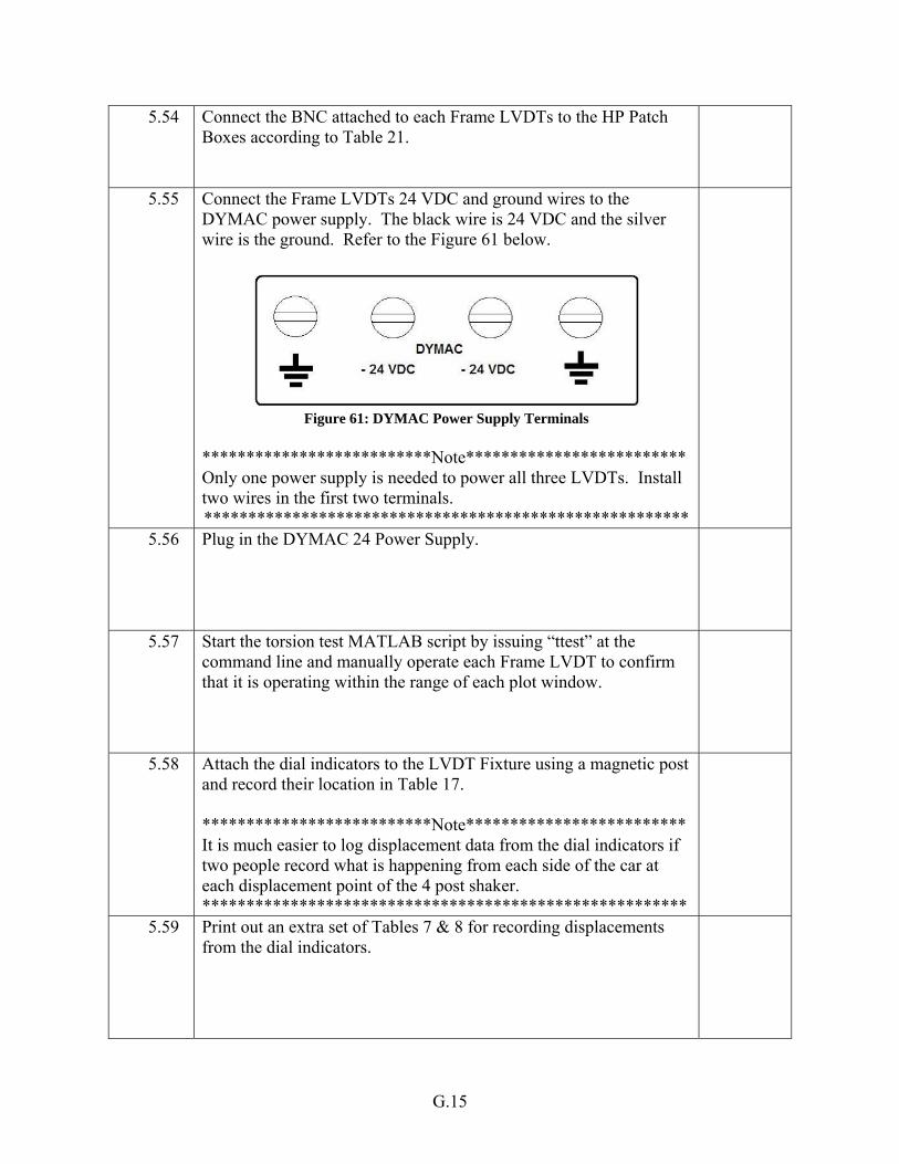
G.15
5.54 Connect the BNC attached to each Frame LVDTs to the HP Patch Boxes according to Table 21.
5.55 Connect the Frame LVDTs 24 VDC and ground wires to the DYMAC power supply. The black wire is 24 VDC and the silver wire is the ground. Refer to the Figure 61 below.
Figure 61: DYMAC Power Supply Terminals
**************************Note************************* Only one power supply is needed to power all three LVDTs. Install two wires in the first two terminals. *******************************************************
5.56 Plug in the DYMAC 24 Power Supply.
5.57 Start the torsion test MATLAB script by issuing “ttest” at the command line and manually operate each Frame LVDT to confirm that it is operating within the range of each plot window.
5.58 Attach the dial indicators to the LVDT Fixture using a magnetic post and record their location in Table 17. **************************Note************************* It is much easier to log displacement data from the dial indicators if two people record what is happening from each side of the car at each displacement point of the 4 post shaker. *******************************************************
5.59 Print out an extra set of Tables 7 & 8 for recording displacements from the dial indicators.

G.16
5.60 Zero the strain gage amps by turning the “Balance” knob so that the red lights are not on and the display reads very close to zero if not zero.
5.61 Start the video camera recording.
5.62 Start the MATLAB torsion test script by issuing “ttest” at the command line.
5.63 Record the external readout of SHAKER LVDT 25 & 26 below: SHAKER LVDT 25 External Position:_________________ SHAKER LVDT 26 External Position:_________________
5.64 With the test conductor in the control room, begin the first test as outlined in Table 18 by moving the setpoint in 0.020” increments. Record the deflection from the dial indicators at every increment position in Table 18.
5.65 Save the MATLAB workspace to a file with the formatted name: “TSMM_CARNAME_DATE_20_MIL.mat.”
5.66 Save the MATLAB display with the formatted name: “TSMM_CARNAME_DATE_20_MIL.fig.”
5.67 Unload the frame in four 0.050” increments until the neutral positions recorded in step 5.61 are achieved.

G.17
5.68 Pause the video recorder.
5.69 Re-zero the dial indicators.
5.70 Re-zero the strain gage amps.
5.71 Start the video camera recording.
5.72 Start the MATLAB torsion test script by issuing “ttest” at the command line.
5.73 Record the external readout of SHAKER LVDT 25 & 26 below: SHAKER LVDT 25 External Position:_________________ SHAKER LVDT 26 External Position:_________________
5.74 With the test conductor in the control room, begin the second test as outline in Table 19. Record the deflection from the dial indicators at every increment position in Table 19.
5.75 Save the MATLAB workspace to a file with the formatted name: “TSMM_CARNAME_DATE_50_MIL.mat.”
5.76 Save the MATLAB display with the formatted name: “TSMM_CARNAME_DATE_50_MIL.fig.”

G.18
5.77 Pause the video recorder
5.78 Unload the frame in four 0.050” increments until the neutral positions recorded in step 5.73 are achieved.
5.79 Make a backup copy of the data files and figures onto a removable media storage device.
5.80 Roll the two red cherry pickers back into their previous positions, install the straps and jack the cherry pickers up until the straps are taught.
5.81 Remove the pivot bolt from each Load Cylinder.
5.82 ******************Three Person Operation****************** With a person in between two shaker posts jack up each cherry picker simultaneously until the Hub Adapters are clear of all the Load Cylinders. **************************Note************************* The person in the middle of the shakers should have a hand on the frame to stabilize it once the Hub Adapters clear the Load Cylinders.
5.83 Turn off the hydraulic pressure to the shakers by using the software in the control room
5.84 Unplug and detach all instrumentation that is attached to the LVDT fixture. Coil and tape all instrumentation wires and store the instrumentation in the frame cabinet.

G.19
5.85 Remove the LVDT fixture from underneath the car and place it along side the railing in the high bay.
5.86 Unplug and coil the Load Cylinder cables from the Vishay Strain Gage Amps and place them with each post so they can move together. **********************WARNING*********************** Make sure to support each wire so that its weight is not pulling on the strain gage. *******************************************************
5.87 Attach the air supply to each shaker post and float the post out of the way to make room for the rolling cart.
5.88 Roll the cart underneath the car.
5.89 Remove the security straps from the frame to the lift arms and store the straps in the high bay cabinet.
5.90 Lower the car onto the rolling cart, detach the straps on the cherry picker and store the cherry pickers where they were located previously.
5.91 Roll the car/cart out from the testing area.
5.92 Remove each solid shock assembly from the suspension system and replace with the bagged hardware.

G.20
5.93 Remove and properly store all TSMM fixturing and hardware back in the frame cabinet.
5.94 Return the VXI mainframe, patch boxes, DYMAC power supply, and PC to the vibrations lab.
5.95 Turn off the Vishay 2100 Strain Gage Amplifier System.
5.96 Install the center cover of each wheel pan back onto each post.
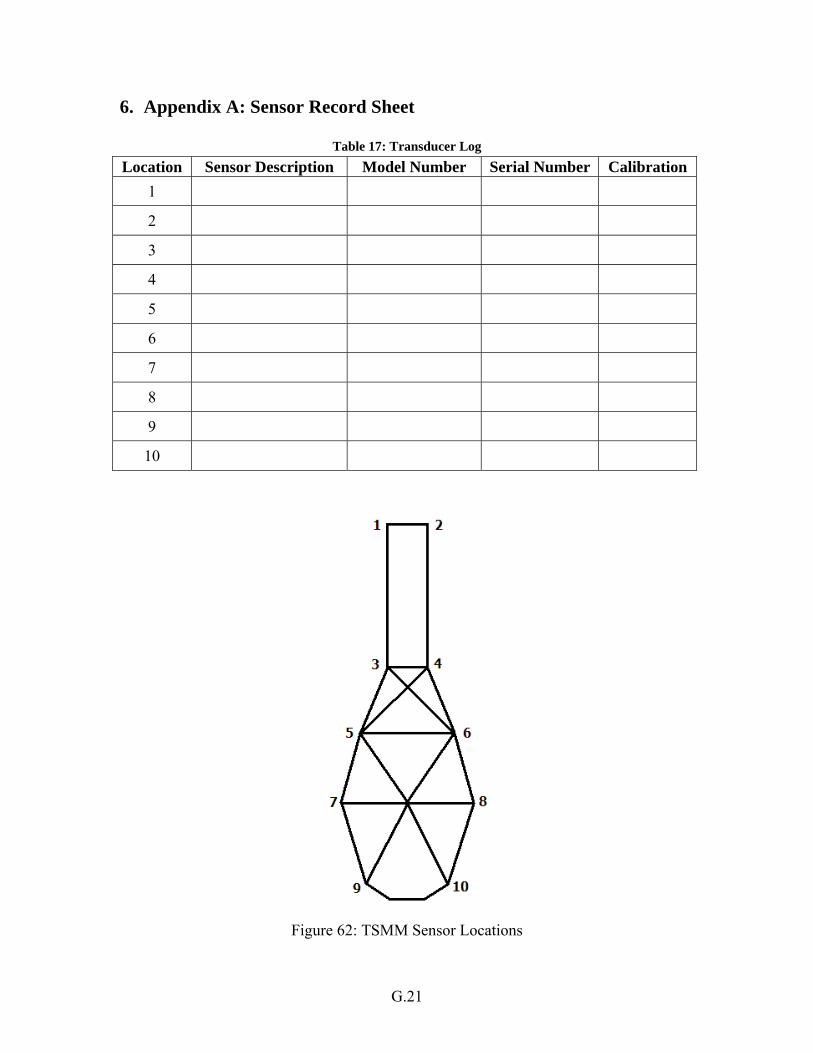
G.21
6. Appendix A: Sensor Record Sheet
Table 17: Transducer Log
Figure 62: TSMM Sensor Locations
Location Sensor Description Model Number Serial Number Calibration 1
2
3
4
5
6
7
8
9
10
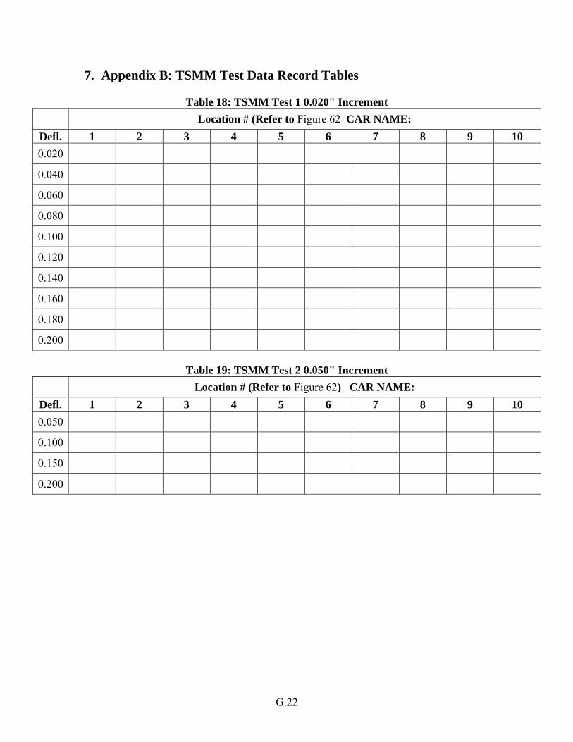
G.22
7. Appendix B: TSMM Test Data Record Tables
Table 18: TSMM Test 1 0.020" Increment Location # (Refer to Figure 62 CAR NAME:
Defl. 1 2 3 4 5 6 7 8 9 10 0.020
0.040
0.060
0.080
0.100
0.120
0.140
0.160
0.180
0.200
Table 19: TSMM Test 2 0.050" Increment Location # (Refer to Figure 62) CAR NAME:
Defl. 1 2 3 4 5 6 7 8 9 10 0.050
0.100
0.150
0.200
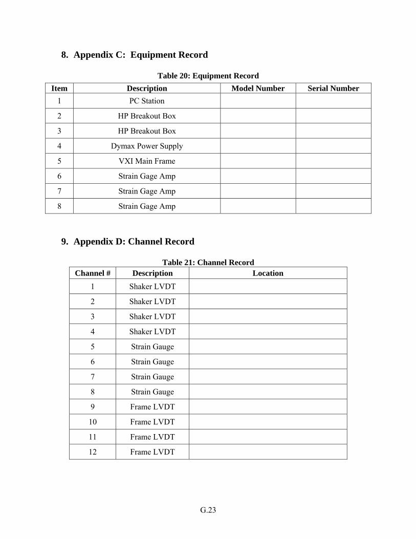
G.23
8. Appendix C: Equipment Record
Table 20: Equipment Record
9. Appendix D: Channel Record
Table 21: Channel Record Channel # Description Location
1 Shaker LVDT
2 Shaker LVDT
3 Shaker LVDT
4 Shaker LVDT
5 Strain Gauge
6 Strain Gauge
7 Strain Gauge
8 Strain Gauge
9 Frame LVDT
10 Frame LVDT
11 Frame LVDT
12 Frame LVDT
Item Description Model Number Serial Number 1 PC Station 2 HP Breakout Box 3 HP Breakout Box 4 Dymax Power Supply 5 VXI Main Frame 6 Strain Gage Amp 7 Strain Gage Amp 8 Strain Gage Amp
![SMC 4133 AUTOMOTIVE STRUCTURES DESIGN FOR BODY TORSIONarahim/L5-BODY TORSION [Compatibility Mode].pdf · - Torsional stiffness = 12000 Nm/deg - Torsion strength = 6250 Nm. SMC 4133](https://img.pdfslide.us/doc/110x75/5e8ab1cc11a90154c430005e/smc-4133-automotive-structures-design-for-body-arahiml5-body-torsion-compatibility.jpg)