Embed Size (px)
Citation preview
Torque Modeling and Control of aVariable Compression Engine
Master’s thesisperformed in Vehicular Systems
byAndreas Bergstrom
Reg nr: LiTH-ISY-EX-3421-2003
29th April 2003

Torque Modeling and Control of a VariableCompression Engine
Master’s thesis
performed in Vehicular Systems,Dept. of Electrical Engineering
at Linkopings universitet
by Andreas Bergstrom
Reg nr: LiTH-ISY-EX-3421-2003
Supervisor: Per AnderssonLinkopings Univeristet
Examiner: Assistant professor Lars ErikssonLinkopings Universitet
Linkoping, 29th April 2003

Avdelning, InstitutionDivision, Department
DatumDate
Sprak
Language
� Svenska/Swedish
� Engelska/English
�
RapporttypReport category
� Licentiatavhandling
� Examensarbete
� C-uppsats
� D-uppsats
� Ovrig rapport
�URL for elektronisk version
ISBN
ISRN
Serietitel och serienummerTitle of series, numbering
ISSN
Titel
Title
ForfattareAuthor
SammanfattningAbstract
NyckelordKeywords
The SAAB variable compression engine is a new engine concept thatenables the fuel consumption to be radically cut by varying the com-pression ratio. A challenge with this new engine concept is that thecompression ratio has a direct influence on the output torque, whichmeans that a change in compression ratio also leads to a change in thetorque. A torque change may be felt as a jerk in the movement of thecar, and this is an undesirable effect since the driver has no control overthe compression ratio.
The aim of this master’s thesis work is to develop a torque controlstrategy for the SAAB variable compression engine. Where the maincontrol objective is to make the output torque behave in a desirableway despite the influence of compression ratio changes.
The controller is developed using a design method called InternalModel Control, which is a straightforward way of both configuring acontroller and determining its parameters. The controller has been im-plemented and evaluated in a real engine, and has proved to be able toreduce the effect of compression ratio disturbance.
Vehicular Systems,Dept. of Electrical Engineering581 83 Linkoping
29th April 2003
—
LITH-ISY-EX-3421-2003
—
http://www.vehicular.isy.liu.sehttp://www.ep.liu.se/exjobb/isy/2003/3421/
Torque Modeling and Control of a Variable Compression Engine
Momentmodellering och momentreglering av en variabelkompressions-motor
Andreas Bergstrom
××
Torque control, SVC, Variable compression, IMC, MVEM

Abstract
The SAAB variable compression engine is a new engine concept thatenables the fuel consumption to be radically cut by varying the com-pression ratio. A challenge with this new engine concept is that thecompression ratio has a direct influence on the output torque, whichmeans that a change in compression ratio also leads to a change in thetorque. A torque change may be felt as a jerk in the movement of thecar, and this is an undesirable effect since the driver has no control overthe compression ratio.
The aim of this master’s thesis work is to develop a torque controlstrategy for the SAAB variable compression engine. Where the maincontrol objective is to make the output torque behave in a desirableway despite the influence of compression ratio changes.
The controller is developed using a design method called InternalModel Control, which is a straightforward way of both configuring acontroller and determining its parameters. The controller has been im-plemented and evaluated in a real engine, and has proved to be able toreduce the effect of compression ratio disturbance.
Keywords: Torque control, SVC, Variable compression, IMC, MVEM
v
Preface
This master’s thesis has been performed at Vehicular Systems, LinkopingUniversity during fall/winter 2002/2003.
Thesis Outline
The work done during this thesis is described in the following chapters.
• Chapter 1 Introduction. Introduction to the thesis
• Chapter 2 Theory. An overview of the basic theory for combustionengines, model building and control theory.
• Chapter 3 The Variable Compression Concept. Here the ideasbehind the variabel compression concept is presented.
• Chapter 4 Engine Model. Presentation of the developed modeland the simulation results.
• Chapter 5 Preliminary Study. Short investigation of which signalsthat are suitable to use and calculations of important transferfunctions.
• Chapter 6 Control Algorithms. Presentation of the developedcontrol algorithm and the results from the evaluation.
• Chapter 7 Conclusions and Future Work. Conclusions and topicsfor future studies
Acknowledgment
I would like to thank everyone at Vehicular Systems for a nice andstimulating time, especially my supervisor Per Andersson for his en-couragement and valuable ideas. Further, I would like to thank MartinGunnarsson for all help in the lab, and also Christer Rosenquist forhelp with the real time system.
Andreas BergstromLinkoping, April 2003
vi
Notation
Nomenclature
Symbol Quantity Unit(AF
)Air-to-fuel ratio -
M Engine Torque NmMnet Net Torque NmMc Combustion torque NmMi Ignition angle torque NmMf Friction torque NmMp Pumping torque Nmmac Air flow into cylinder kg/smat Air flow past throttle kg/smf Fuel flow into cylinder kg/smi Change of mass in the intake manifold kg/sN Engine speed rpmpe Pressure in the exhaust manifold Papi Pressure in the intake manifold Paqhv Heating value J/kgR Gas constant J/(kg ·K)rc Compression ratio -Ti Intake manifold temperature KVi Intake manifold volume m3
Vd Displaced volume m3
Vc Clearance volume m3
γ Ratio of specific heat -ηvol Volumetric efficiency -θign Ignition Angle degreeλ Air -to-fuel equivalence ratio (normalized
(AF
)) -
τth Throttle time constant sτr Compression ratio time constant s
Abbreviations
Abbreviation ExplanationBDC Bottom Dead CenterIMC Internal Model ControlMEP Mean Effective PressureMVEM Mean Value Engine ModelSI Spark IgnitedSVC SAAB Variable CompressionTDC Top Dead Center
vii

viii
Contents
Abstract v
Preface and Acknowledgment vii
Notation viii
1 Introduction 11.1 Objectives . . . . . . . . . . . . . . . . . . . . . . . . . . 21.2 Methods . . . . . . . . . . . . . . . . . . . . . . . . . . . 21.3 Target Group . . . . . . . . . . . . . . . . . . . . . . . . 3
2 Theory 52.1 Engine Introduction . . . . . . . . . . . . . . . . . . . . 5
2.1.1 Four stroke cycle . . . . . . . . . . . . . . . . . . 62.2 Model Building . . . . . . . . . . . . . . . . . . . . . . . 72.3 Control Theory . . . . . . . . . . . . . . . . . . . . . . . 7
2.3.1 The Transfer Functions of the Closed Loop System 8
3 The Variable Compression Concept 93.1 Downsizing . . . . . . . . . . . . . . . . . . . . . . . . . 93.2 Supercharging . . . . . . . . . . . . . . . . . . . . . . . . 103.3 Variable compression . . . . . . . . . . . . . . . . . . . . 103.4 SAAB Variable Compression Engine . . . . . . . . . . . 11
4 Engine Model 134.1 Model Overview . . . . . . . . . . . . . . . . . . . . . . 134.2 Main throttle . . . . . . . . . . . . . . . . . . . . . . . . 144.3 Intake Manifold . . . . . . . . . . . . . . . . . . . . . . . 15
4.3.1 Dynamic Pressure Model . . . . . . . . . . . . . 154.3.2 Engine Mass Flow Model . . . . . . . . . . . . . 164.3.3 Fuel Injection . . . . . . . . . . . . . . . . . . . . 19
4.4 Cylinders . . . . . . . . . . . . . . . . . . . . . . . . . . 194.4.1 Combustion . . . . . . . . . . . . . . . . . . . . . 204.4.2 Pumping losses . . . . . . . . . . . . . . . . . . . 21
ix
4.4.3 Friction losses . . . . . . . . . . . . . . . . . . . . 214.4.4 Ignition Angle . . . . . . . . . . . . . . . . . . . 22
4.5 Compression Ratio . . . . . . . . . . . . . . . . . . . . . 224.6 Model Summary . . . . . . . . . . . . . . . . . . . . . . 224.7 Model Implementation . . . . . . . . . . . . . . . . . . . 244.8 Model Validation . . . . . . . . . . . . . . . . . . . . . . 25
4.8.1 Stationary Validation . . . . . . . . . . . . . . . 254.8.2 Dynamic Validation . . . . . . . . . . . . . . . . 26
5 Preliminary Study 295.1 Controller Signals . . . . . . . . . . . . . . . . . . . . . . 29
5.1.1 Air-Flow Past Throttle . . . . . . . . . . . . . . 295.1.2 Ignition Angle . . . . . . . . . . . . . . . . . . . 295.1.3 Compression Ratio . . . . . . . . . . . . . . . . . 305.1.4 Torque . . . . . . . . . . . . . . . . . . . . . . . . 305.1.5 Summary . . . . . . . . . . . . . . . . . . . . . . 30
5.2 Transfer Function . . . . . . . . . . . . . . . . . . . . . . 31
6 Control Algorithm 336.1 Control Demands . . . . . . . . . . . . . . . . . . . . . . 336.2 Control Structure . . . . . . . . . . . . . . . . . . . . . . 346.3 Control Design . . . . . . . . . . . . . . . . . . . . . . . 34
6.3.1 How to Choose the Design Method? . . . . . . . 356.3.2 Internal Model Control (IMC) . . . . . . . . . . 356.3.3 Controller Calculations . . . . . . . . . . . . . . 37
6.4 Observer . . . . . . . . . . . . . . . . . . . . . . . . . . . 406.5 Evaluation . . . . . . . . . . . . . . . . . . . . . . . . . . 40
6.5.1 Evaluation of Observer . . . . . . . . . . . . . . . 416.5.2 Evaluation of the Controller . . . . . . . . . . . . 42
7 Conclusions and Future Work 477.1 Summary . . . . . . . . . . . . . . . . . . . . . . . . . . 477.2 Accomplishments and Conclusion . . . . . . . . . . . . . 487.3 Future Work . . . . . . . . . . . . . . . . . . . . . . . . 48
References 51
A Ignition Angle Measurements 53
B Model Parameters 55
C SIMULINK Implementation 57
x
Chapter 1
Introduction
SAAB has developed a new engine concept called SVC (SAAB Vari-able Compression), this new engine concept enables fuel consumptionto be radically cut, but without impairing engine performance. TheSVC engine has variable compression i.e. variable size of the clearancevolume. This alone adds a new control input that affects every aspectof engine control. The engine is also equipped with a compressor forsupercharging, with some additional associated control inputs.
One challenge with this new concept is that the compression ratiohas a direct influence on the output torque. This is a problem becausethe engine then can change its characteristics under operation, and thisinfluences the driveability of the car. A big change in the compressionratio can even be felt by the driver as a jerk in movement. Anotherproblem is that the connection and disconnection of the mechanical su-percharger also have a direct influence on the engine torque, and suddenconnection and disconnection can also be felt as jerks in movement.
So in order to fully take advantage of the benefits of this new engineconcept, it is necessary to have some sort of torque control that cankeep a constant torque regardless of these disturbances. This thesisconcentrates on finding a solution to the problem with the compressionratio changes.
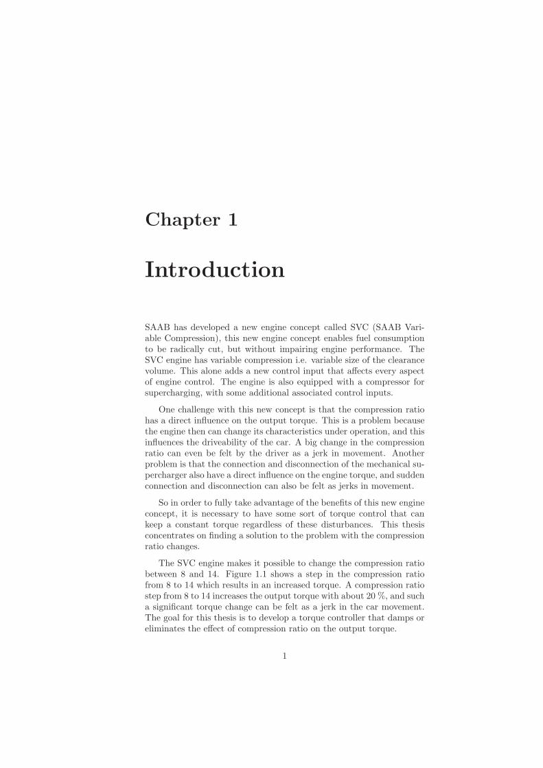
The SVC engine makes it possible to change the compression ratiobetween 8 and 14. Figure 1.1 shows a step in the compression ratiofrom 8 to 14 which results in an increased torque. A compression ratiostep from 8 to 14 increases the output torque with about 20 %, and sucha significant torque change can be felt as a jerk in the car movement.The goal for this thesis is to develop a torque controller that damps oreliminates the effect of compression ratio on the output torque.
1
2 Introduction
6 8 10 12 14 16
8
10
12
14
Time [s]
Com
pres
sion
rat
io
6 8 10 12 14 1635
40
45
50
55
60
65
70
Time [s]
Tor
que
[Nm
]
Figure 1.1: Shows how the output torque changes when the compressionratio changes from 8 to 14, at 2000 rpm. The top plot shows thecompression ratio and the bottom plot shows the output torque.
1.1 Objectives
There are three objectives for this thesis. The objectives are to:
• Develop a torque model for the the SVC engine with the inputsignals air mass flow past throttle, compression ratio and ignitionangle.
• Develop and evaluate one or more torque control strategies in themodel.
• Evaluate the control strategies on a real SVC engine in the enginelab.
1.2 Methods
The model and control strategies have been developed and implementedin an MATLAB and SIMULINK environment. The necessary data collec-tion for the model and evaluation of the control strategies has been

1.3. Target Group 3
performed in an engine test cell in Vehicular Systems’ research labora-tory, using a measurement system combined with a real time system.
1.3 Target Group
This thesis is aimed for engineers and students, with basic knowledgein the areas of vehicular systems and control theory.

4
Chapter 2
Theory
In this chapter some theoretical background to the subject areas in thisthesis will be given. An introduction to how a four cycle combustionengine works is presented in section 2.1. In section 2.2 and 2.3 somebasic principles for model building and control theory is covered.
2.1 Engine Introduction
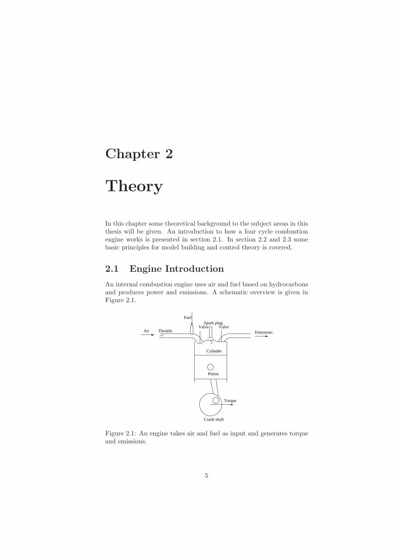
An internal combustion engine uses air and fuel based on hydrocarbonsand produces power and emissions. A schematic overview is given inFigure 2.1.
Air Throttle
FuelSpark plug
Valve ValveEmissions
Cylinder
Piston
Crank shaft
Torque
Figure 2.1: An engine takes air and fuel as input and generates torqueand emissions.
5
6 Chapter 2. Theory
Exhaust
Intake Compression Expansion Exhaust
Intake Intake Exhaust ExhaustIntake Intake Exhaust
Figure 2.2: The four strokes intake, compression, expansion and ex-haust of a four stroke engine.
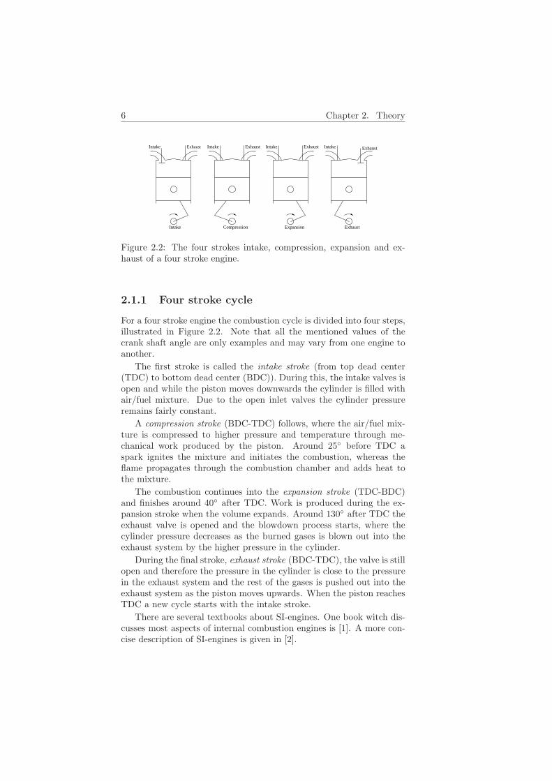
2.1.1 Four stroke cycle
For a four stroke engine the combustion cycle is divided into four steps,illustrated in Figure 2.2. Note that all the mentioned values of thecrank shaft angle are only examples and may vary from one engine toanother.
The first stroke is called the intake stroke (from top dead center(TDC) to bottom dead center (BDC)). During this, the intake valves isopen and while the piston moves downwards the cylinder is filled withair/fuel mixture. Due to the open inlet valves the cylinder pressureremains fairly constant.
A compression stroke (BDC-TDC) follows, where the air/fuel mix-ture is compressed to higher pressure and temperature through me-chanical work produced by the piston. Around 25◦ before TDC aspark ignites the mixture and initiates the combustion, whereas theflame propagates through the combustion chamber and adds heat tothe mixture.
The combustion continues into the expansion stroke (TDC-BDC)and finishes around 40◦ after TDC. Work is produced during the ex-pansion stroke when the volume expands. Around 130◦ after TDC theexhaust valve is opened and the blowdown process starts, where thecylinder pressure decreases as the burned gases is blown out into theexhaust system by the higher pressure in the cylinder.
During the final stroke, exhaust stroke (BDC-TDC), the valve is stillopen and therefore the pressure in the cylinder is close to the pressurein the exhaust system and the rest of the gases is pushed out into theexhaust system as the piston moves upwards. When the piston reachesTDC a new cycle starts with the intake stroke.
There are several textbooks about SI-engines. One book witch dis-cusses most aspects of internal combustion engines is [1]. A more con-cise description of SI-engines is given in [2].
2.2. Model Building 7
uG
yrFr
+
_
Fy
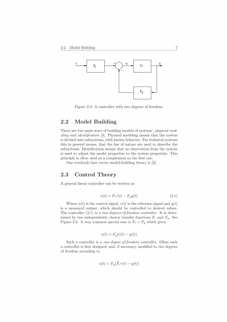
Figure 2.3: A controller with two degrees of freedom.
2.2 Model Building
There are two main ways of building models of systems’, physical mod-eling and identification [3]. Physical modeling means that the systemis divided into subsystems, with known behavior. For technical systemsthis in general means, that the law of nature are used to describe thesubsystems. Identification means that an observation from the systemis used to adjust the model properties to the system properties. Thisprinciple is often used as a complement to the first one.
One textbook that covers model-building theory is [3].
2.3 Control Theory
A general linear controller can be written as
u(t) = Frr(t) − Fyy(t) (2.1)
Where u(t) is the control signal, r(t) is the reference signal and y(t)is a measured output, which should be controlled to desired values.The controller (2.1) is a two-degrees-of-freedom controller. It is deter-mined by two independently chosen transfer functions Fr and Fy. SeeFigure 2.3. A very common special case is Fr = Fy which gives
u(t) = Fy(r(t) − y(t))
Such a controller is a one-degree-of-freedom controller. Often sucha controller is first designed, and, if necessary, modified to two degreesof freedom according to
u(t) = Fy(Frr(t) − y(t))
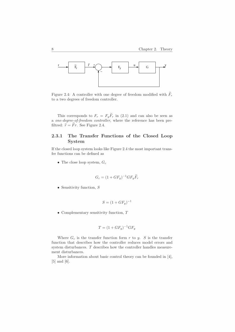
8 Chapter 2. Theory
Fyr
Fr+
_
yG
~ r~ u
Figure 2.4: A controller with one degree of freedom modified with Frto a two degrees of freedom controller.
This corresponds to Fr = FyFr in (2.1) and can also be seen asa one-degree-of-freedom controller, where the reference has been pre-filtred: r = F r. See Figure 2.4.
2.3.1 The Transfer Functions of the Closed LoopSystem
If the closed loop system looks like Figure 2.4 the most important trans-fer functions can be defined as
• The close loop system, Gc
Gc = (1 +GFy)−1GFyFr
• Sensitivity function, S
S = (1 +GFy)−1
• Complementary sensitivity function, T
T = (1 +GFy)−1GFy
Where Gc is the transfer function form r to y. S is the transferfunction that describes how the controller reduces model errors andsystem disturbances. T describes how the controller handles measure-ment disturbances.
More information about basic control theory can be founded in [4],[5] and [6].
Chapter 3
The VariableCompression Concept
Variable compression is a new engine concept that enables fuel con-sumption to be radically cut, but without impairing engine perfor-mance. The variable compression concept contains three cornerstonesdownsizing, supercharging and variable compression [7]. The corner-stones are described in section 3.1, 3.2 and 3.3. One example of avariable compression engine is the SAAB Variable Compression (SVC)engine, technical data and pictures of the engine is presented in sec-tion 3.4.
3.1 Downsizing
An Otto engine is most efficient and uses the energy in the fuel at itsmaximum when it is running at high load. A small engine must workharder and must thus run to its almost full load if it is to perform thesame work as a bigger engine that utilizes only part of its maximumcapacity during normal operation.
One of the reasons is that, under these conditions, the pumpinglosses are lower in a small engine. The piston in the cylinder is undera slight vacuum during the intake stroke, when it is drawing air intothe cylinder. The extra energy needed for pulling the piston down isknown as the pumping losses. Since a small engine more frequentlyruns at full load and the throttle is therefore more often fully open, thepumping losses in the small engine are usually lower then they are in abig engine.
Moreover a small engine is lighter and has lower friction. So a smallengine is generally more efficient than a big engine.
9
10 Chapter 3. The Variable Compression Concept
3.2 Supercharging
Although a small engine is efficient, it is not powerful enough in practiceto be used for anything then powering small, lightweight cars, if it is togive the car acceptable performance. By supercharging, which involvesforcing in more air, more fuel can be injected and be burned. Theengine then delivers more power for every piston stroke, which resultsin higher torque and higher engine output. Moreover if the engine issupercharged only at large throttle openings when extra power is reallyneeded, the fuel economy of the small engine can be combined with thepreformance of a big engine.
3.3 Variable compression
In [1] compression ratio, rc, is defined as
rc =Vd + VcVc
Where Vd is the displaced volume and Vc is the clerance volume. Inother words, the amount by witch the fuel/air mixture is compressedin the cylinder before it is ignited. The compression ratio is one of themost important factors that determine how efficiently the engine canutilize the energy in the fuel. For an ideal Otto cycle the theoreticalefficiency is [1]
η = 1 − 1rγ−1c
Where γ is ratio of specific heats. For an SI-engine operating atstoichiometric mixture γ ≈ 1.3.
As a general rule, the energy in the fuel will be better utilized ifthe compression ratio is as high as possible. Current engines have acompression ratio around 10, and the question is why is it not higher.This is because [2]:
• If the compression ratio is to high the air/fuel mixture are exposedto higher temperatures, the fuel will auto ignite, giving rise toknocking, which could damage the engine.
• Increased heat transfer to the combustion chamber walls due tosmall clearance volume.
• Increased friction losses and emission of unburned hydrocarbons.
3.4. SAAB Variable Compression Engine 11
In a conventional engine, the maximum compression ratio witch theengine can withstand is therefore set by the conditions in the cylinderat high load, when the fuel and air consumption is at maximum. Thecompression ratio remains the same when the engine is running at lowload.
The basic idea of variable compression is simple: Use high compres-sion ratio during low load for high efficiency, and as the load increasesthe compression ratio is decreased to match the knocking.
3.4 SAAB Variable Compression Engine
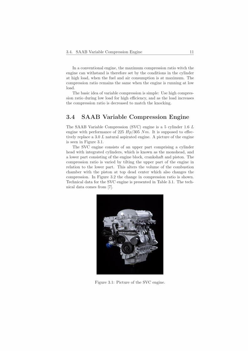
The SAAB Variable Compression (SVC) engine is a 5 cylinder 1.6 Lengine with performance of 225 Hp/305 Nm. It is supposed to effec-tively replace a 3.0 L natural aspirated engine. A picture of the engineis seen in Figure 3.1.
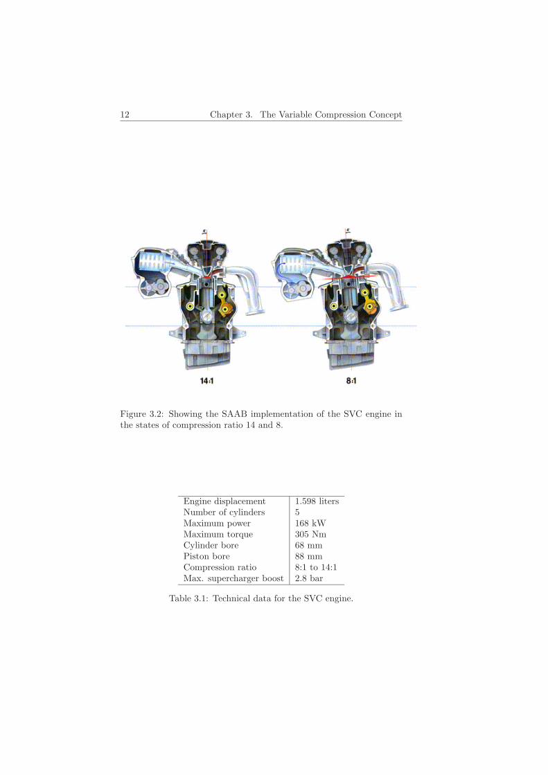
The SVC engine consists of an upper part comprising a cylinderhead with integrated cylinders, which is known as the monohead, anda lower part consisting of the engine block, crankshaft and piston. Thecompression ratio is varied by tilting the upper part of the engine inrelation to the lower part. This alters the volume of the combustionchamber with the piston at top dead center which also changes thecompression. In Figure 3.2 the change in compression ratio is shown.Technical data for the SVC engine is presented in Table 3.1. The tech-nical data comes from [7].
Figure 3.1: Picture of the SVC engine.
12 Chapter 3. The Variable Compression Concept
Figure 3.2: Showing the SAAB implementation of the SVC engine inthe states of compression ratio 14 and 8.
Engine displacement 1.598 litersNumber of cylinders 5Maximum power 168 kWMaximum torque 305 NmCylinder bore 68 mmPiston bore 88 mmCompression ratio 8:1 to 14:1Max. supercharger boost 2.8 bar
Table 3.1: Technical data for the SVC engine.
Chapter 4
Engine Model
In order to develop control algorithms it was decided that a computermodel of the system should be developed. This is because:
• Creating a model of the system is a good way of gathering knowl-edge about the system. The work with the building of the modelprovides a structured way of gathering the information that isneeded for a successful control design.
• Some control designs like Internal Model Control demands a sys-tem model.
• If most of trial and error work can be performed on the computermodel, much expensive time on the engine test test bench can besaved.
The model shall describe the torque from the input signals air massflow past throttle, compression ratio and ignition angle, and will bedeveloped with help of physical model building. The engine model de-scribed in this chapter is a mean value engine model (MVEM). MVEMmeans that no variations within cycles are covered and makes the modelvalid only for time intervals far greater than one engine cycle.
4.1 Model Overview
A schematic overview of the engine with surrounding devices is given inFigure 4.1. When modeling an SI-engine by using physical modeling,it is beneficial to divide the engine in distinct subsystems.
The amount of air entering the engine is governed primary by themain throttle. The mass flow dynamics over the main throttle is de-scribed in section 4.2. After the main throttle the air comes to theby-pass throttle. When the supercharger is on the by-pass throttle
13
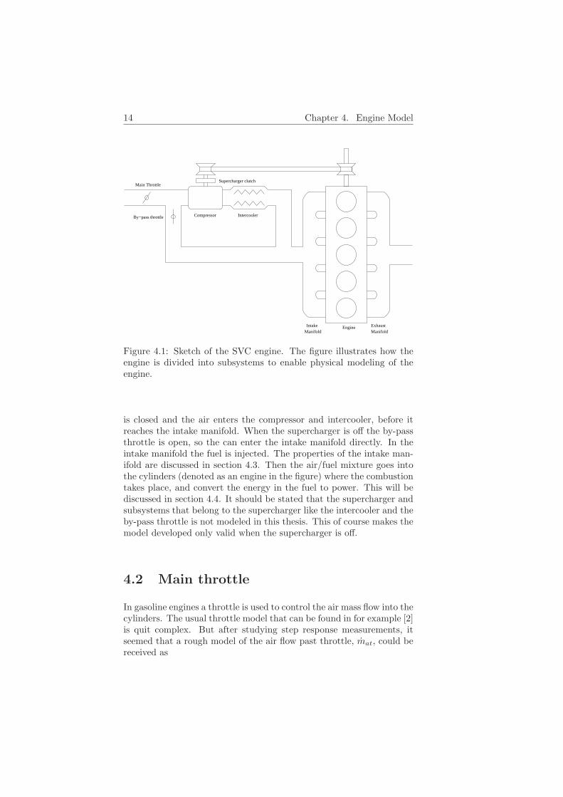
14 Chapter 4. Engine Model
ManifoldIntake
ManifoldExhaustEngine
IntercoolerCompressor
Main ThrottleSupercharger clutch
By−pass throttle
Figure 4.1: Sketch of the SVC engine. The figure illustrates how theengine is divided into subsystems to enable physical modeling of theengine.
is closed and the air enters the compressor and intercooler, before itreaches the intake manifold. When the supercharger is off the by-passthrottle is open, so the can enter the intake manifold directly. In theintake manifold the fuel is injected. The properties of the intake man-ifold are discussed in section 4.3. Then the air/fuel mixture goes intothe cylinders (denoted as an engine in the figure) where the combustiontakes place, and convert the energy in the fuel to power. This will bediscussed in section 4.4. It should be stated that the supercharger andsubsystems that belong to the supercharger like the intercooler and theby-pass throttle is not modeled in this thesis. This of course makes themodel developed only valid when the supercharger is off.
4.2 Main throttle
In gasoline engines a throttle is used to control the air mass flow into thecylinders. The usual throttle model that can be found in for example [2]is quit complex. But after studying step response measurements, itseemed that a rough model of the air flow past throttle, mat, could bereceived as
4.3. Intake Manifold 15
dmat
dt= − 1
τthmat +
1τth
sat matref
where the function sat describes a saturation, and defined by
sat matref =
mmax if matref > mmax
matref if mmin ≤ matref ≤ mmax
mmin if matref < mmin
Where τth = 0.075, mmax = 0.07 kg/s, mmin = 0.003 kg/s andmatref is a reference signal for the air flow. Worth noting is that thetime constant, τth, and the saturation boundaries, mmax and mmin,actually depends on the engine speed, N . But test shows that τth =0.075, mmax = 0.07 kg/s and mmin = 0.003 kg/s give an adequatelyaccurate result. The throttle also contains a time delay of about 0.40 s.
4.3 Intake Manifold
The air transport in the intake manifold depends on
• The throttle and the air flow past it.
• The amount of air that goes into the cylinder.
• The pressure in the intake manifold.
4.3.1 Dynamic Pressure Model
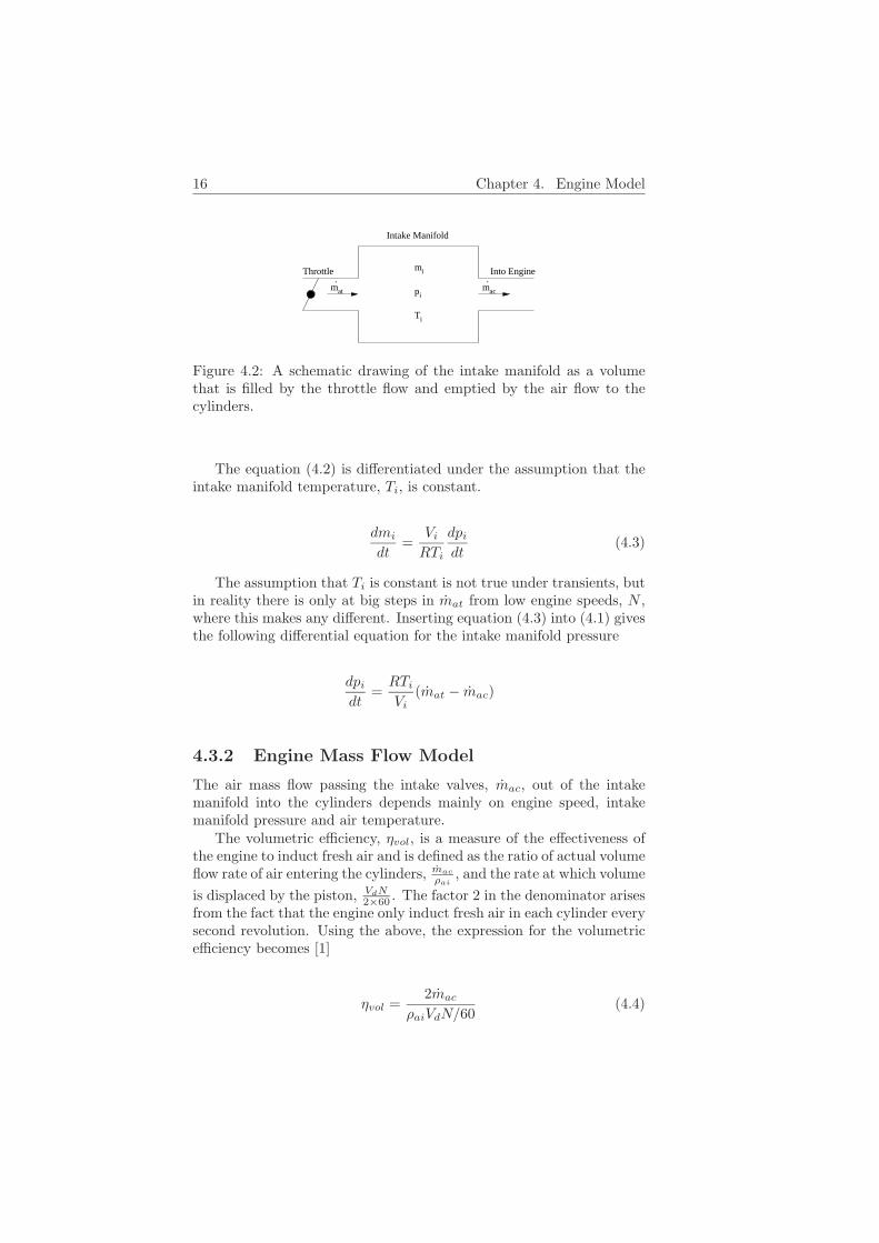
A model of the pressure build-up in the intake manifold is obtained byapplying a balance equation expressing the conversion of mass in themanifold [8], see Figure 4.2. The increase or decrease of mass in theintake manifold, mi, is determined by the air flow past the throttle,mat, and the air flow into the cylinder, mac. This can be expressed as
dmi
dt= mat − mac (4.1)
Using the ideal gas law pV = mRT ⇒ m = pVRT , on mi in equa-
tion (4.1) can be expressed in terms of the intake manifold pressure, pi,in following way
mi =ViRTi
pi (4.2)
16 Chapter 4. Engine Model
mi
pi
Ti
mat
.mac
.Throttle
Intake Manifold
Into Engine
Figure 4.2: A schematic drawing of the intake manifold as a volumethat is filled by the throttle flow and emptied by the air flow to thecylinders.
The equation (4.2) is differentiated under the assumption that theintake manifold temperature, Ti, is constant.
dmi
dt=
ViRTi
dpidt
(4.3)
The assumption that Ti is constant is not true under transients, butin reality there is only at big steps in mat from low engine speeds, N ,where this makes any different. Inserting equation (4.3) into (4.1) givesthe following differential equation for the intake manifold pressure
dpidt
=RTiVi
(mat − mac)
4.3.2 Engine Mass Flow Model
The air mass flow passing the intake valves, mac, out of the intakemanifold into the cylinders depends mainly on engine speed, intakemanifold pressure and air temperature.
The volumetric efficiency, ηvol, is a measure of the effectiveness ofthe engine to induct fresh air and is defined as the ratio of actual volumeflow rate of air entering the cylinders, mac
ρai, and the rate at which volume
is displaced by the piston, VdN2×60 . The factor 2 in the denominator arises
from the fact that the engine only induct fresh air in each cylinder everysecond revolution. Using the above, the expression for the volumetricefficiency becomes [1]
ηvol =2mac
ρaiVdN/60(4.4)
4.3. Intake Manifold 17
If one again uses the ideal gas law pV = mRT ⇒ ρ = mv = p
RT theair density in the inlet, ρai, can be calculated as
ρai =piRTi
(4.5)
If inserting equation (4.5) into (4.4) the airflow into the cylinders,mac, can be expressed as
mac = ηvolpiVdN/60
2RTi(4.6)
Where the volumetric efficiency depends on engine speed, intakemanifold pressure and compression ratio, ηvol(N, pi, rc). In order todetermine ηvol(N, pi, rc) it is common to measure it and map it overthe engine’s operating range by running stationary tests. But accordingto [9] can ηvol · pi be described as s0pi + s1 for fixed compressions. Ifusing ηvolpi = s0pi+ s1 in equation (4.6) the airflow into the cylinders,mac, can be described as
mac = (s0pi + s1)VdN/602RTi
(4.7)
Mass Flow Measurements
In order to determine s0 and s1, experiments were pi, Ti, N and mat
was measured stationary for different intake manifold pressures andcompression ratios. ηvol · pi can be calculated from the measurementsas ηvol = mac
120RTi. Note that for stationary conditions, no mass is stored
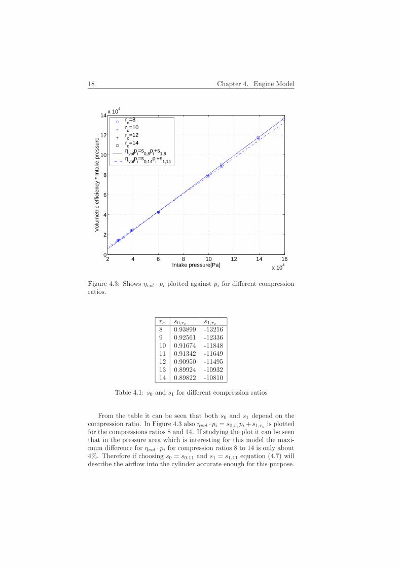
in the manifold so that the air mass flow into the cylinders equalsthe air past the throttle and thus mac = mat. In Figure 4.3 ηvol · piis plotted against pi for different compression ratios (circles, x-marks,pluses and squares in the figure). From this figure s0 and s1 for differentcompression ratios can be calculated and presented in Table 4.1.
18 Chapter 4. Engine Model
2 4 6 8 10 12 14 16
x 104
0
2
4
6
8
10
12
14x 10
4
Intake pressure[Pa]
Vol
umet
ric e
ffici
ency
* In
take
pre
ssur
e
rc=8
rc=10
rc=12
rc=14
ηvol
pi=s
0,8p
i+s
1,8η
volp
i=s
0,14p
i+s
1,14
Figure 4.3: Shows ηvol · pi plotted against pi for different compressionratios.
rc s0,rcs1,rc
8 0.93899 -132169 0.92561 -1233610 0.91674 -1184811 0.91342 -1164912 0.90950 -1149513 0.89924 -1093214 0.89822 -10810
Table 4.1: s0 and s1 for different compression ratios
From the table it can be seen that both s0 and s1 depend on thecompression ratio. In Figure 4.3 also ηvol · pi = s0,rc
pi+ s1,rcis plotted
for the compressions ratios 8 and 14. If studying the plot it can be seenthat in the pressure area which is interesting for this model the maxi-mum difference for ηvol · pi for compression ratios 8 to 14 is only about4%. Therefore if choosing s0 = s0,11 and s1 = s1,11 equation (4.7) willdescribe the airflow into the cylinder accurate enough for this purpose.
4.4. Cylinders 19
4.3.3 Fuel Injection
In order to inject the correct amount of fuel into the engine, it is nec-essary to know the theoretical proportions of air and fuel, i.e. theremust be enough air to oxidize the fuel perfectly. This ratio is called thestoichiometric air to fuel ratio [1]
(A
F
)s
=(mac
mf
)s
The petrol used in the laboratory has(AF
)s≈ 15.
An interesting property is the ratio between the true air to fuelratio,
(AF
), and
(AF
)s
λ =
(AF
)(AF
)s
It essential to keep λ close to one in order to maintain good catalystfunction. It is only possible to have λ = 1 if
(AF
)=
(AF
)s
and asa consequence we must have the following relation between the massflow of air into the cylinders, mac, and the mass flow of fuel into thecylinders, mf
mf =115mac
4.4 Cylinders
In the cylinders the combustion process takes place, and convert theenergy in the fuel to power. The combustion process is very complicatedand a simple of model for the torque is present below. The engine torquedepends mainly on:
• How the heat stored in the fuel can be converted into torque.
• Torque lost to pumping when the burned mixture is pumped out.
• Torque lost to friction between the piston and walls and frictionlosses in the crank configuration.
• Torque lost to accessories such as compressor, servo pumps, elec-trical generator etc.
20 Chapter 4. Engine Model
If neglect the torque lost to accessories, the net torque, Mnet, can beexpressed as
Mnet = Mc −Mf −Mp
Where Mc is the torque delivered from combustion of the fuel, Mf
and Mp is the torque lost to friction and pumping.
4.4.1 Combustion
The torque is measure of an engine’s ability to do work, power is therate at which work is done. It follows that the power, P , is deliveredby the engine is the product of torque and angular speed [1]
P = 2πMN/60 (4.8)
Ideally all the heat stored in the fuel may be converted to power,in that case the delivered power is given by taking the product of theheating value of the fuel, qhv = 44.3 MJ/kg for isooctane, and thefuel mass flow through the cylinders, mf . However there will be lossesduring the energy conversion, thus we have to multiply with the fuelconversion efficiency, ηf,i
P = ηf,iqhvmfc (4.9)
If equation (4.8) and (4.9) are combined a model for the enginetorque is given as
Mc = ηf,iqhvmfc
2πN/60
If the combustion process is approximated as a Otto cycle or con-stant volume cycle, the ηf,i can be calculated as, See [1]
ηf,i = κ
(1 − 1
rγ−1c
)
Where κ has been introduced because in the calculations aboveenergy losses due to incomplete combustion, heat transfer from gas tothe cylinder walls and timing losses has been neglected. From enginemeasurements of how the total torque changes when the compression,rc, changes, the value of κ was determined to 0.74.
4.4. Cylinders 21
4.4.2 Pumping losses
The piston in the cylinder is under a slight vacuum during the intakestroke, when it is drawing air/fuel into the cylinder. The extra energyneeded for pulling the piston down is known as the pumping losses.
Mean effective pressure (MEP) is define as
MEP =work produced per cycle
volume displaced per cycle
From this the pump mean effective pressure (pMEP) can be calcu-lated as the ratio of the pumping work per cycle, (pe − pi)Vd, See [1],where pe and pi is the pressure in the exhaust and the intake manifold,and the volume displaced per cycle, Vd.
pMEP = pe − pi (4.10)
The mean effective pressure can also be calculated based on workthat the engine produces in a dynamo-meter, See [1].
MEP =2πMnrVd
(4.11)
From equations (4.10) and (4.11) the torque that is lost to the pump-ing, Mp, can be calculated as
Mp =Vd
2πnr(pe − pi)
4.4.3 Friction losses
Friction losses depends mainly on engine speed, N . A common way tomodel the torque that is lost to friction is as follows, see [1]
Mf = AN2 +BN + C
In order to decide the values of the constants A, B and C real enginemeasurements of the torque for different speeds are compared with thetorque from the model for the same speeds. The constants A,B and Care then fitted so torque from the model agreed with the torque fromthe measurements.
22 Chapter 4. Engine Model
4.4.4 Ignition Angle
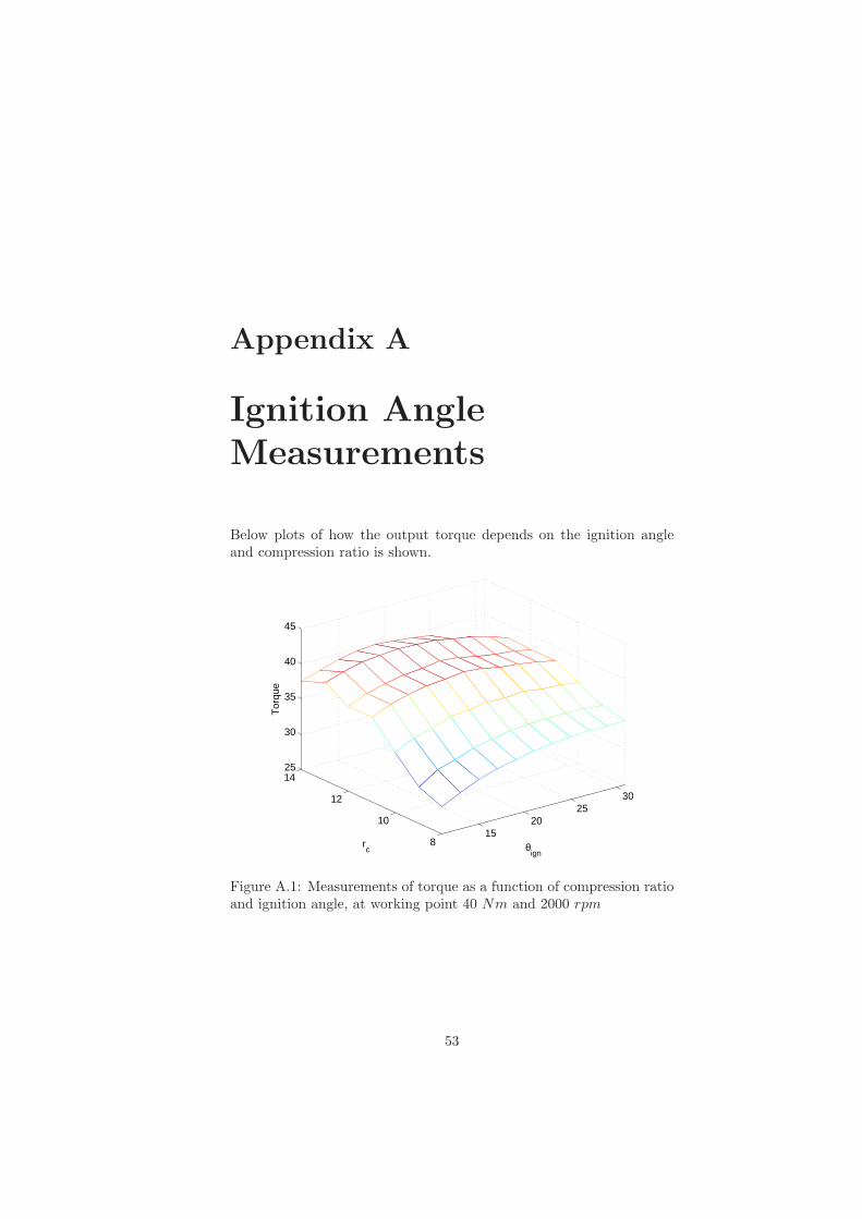
With ignition angle, θign, it is meant the position in crank angles beforeTDC where the spark discharge occurs. The ignition angle has a directinfluence on the engine efficiency and the generated torque. In order todetermine how the torque depends on the ignition angle, experimentswere performed running the engine at a large number of different sparkadvances, compression ratios and torque. See Appendix A for plots.From these experiments a three-dimensional look-up table is imple-mented. The look up table describes the torque, Mi, that is lost fordifferent ignition angle, compression ratios and torque.
Mi = Look-up table(θign, rc,Mnet)
The total output torque then can be calculated as
M = Mnet −Mi
To keep down the number of measurements needed, the ignitionangle is only mapped around operating point 40−80 Nm and at enginespeed 2000 rpm. This means that the ignition angle map is only validaround this working point. For simulations at other operating pointsthe ignition angle map can be disconnected and then the model worksas if the optimal ignition angle is used at all times.
4.5 Compression Ratio
Studying step response measurements it seems like the compressionratio, rc, can be modeled as
drcdt
=1τrc
(−rc + rcref )
Where τrc = 0.40 and rcref is a reference signal for the compressionratio.
4.6 Model Summary
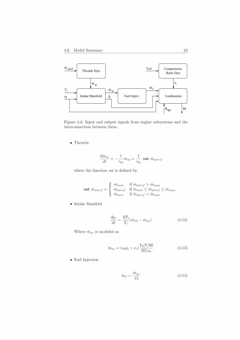
The model is summarized in this section to make it easier to get a com-plete picture of the model equations. In Figure 4.4 there is a schematicoverview of the model, where the arrows indicate the flow of informationthrough the model.
4.6. Model Summary 23
Throttle Dyn.
Intake Manifold Fuel Inject.
m atref.
m at.
iT
Combustion
Ratio Dyn.Compressionrcref
rc
m ac. m f
.
pi
ignθ
N
M
Figure 4.4: Input and output signals from engine subsystems and theinterconnection between them.
• Throttle
dmat
dt= − 1
τthmat +
1τth
sat matref
where the function sat is defined by
sat matref =
mmax if matref > mmax
matref if mmin ≤ matref ≤ mmax
mmin if matref < mmin
• Intake Manifold
dpidt
=RTiVi
(mat − mac) (4.12)
Where mac is modeled as
mac = (s0pi + s1)VdN/60RTinr
(4.13)
• Fuel Injection
mf =mac
15(4.14)
24 Chapter 4. Engine Model
• Compression Ratio
drcdt
=1τr
(−rc + rcref ) (4.15)
• Combustion
Mnet = Mc −Mp −Mf (4.16)
Where Mc is
Mc =12πκ(1 − 1
rγ−1c
)qhvmf
N/60(4.17)
Mp and Mf is
Mp =Vd
2πnr(pe − pi) (4.18)
Mf = AN2 +BN + C (4.19)
And then M is calculated as
M = Mnet −Mi (4.20)
Where Mi is
Mi = Look-up table(θign, rc,Mnet) (4.21)
4.7 Model Implementation
The model is implemented in SIMULINK , which is a software packagefor modeling, simulation and analysis of dynamic systems. SIMULINK isinclude as a toolbox in MATLAB . Both linear and nonlinear systems canbe implemented in continuous and discreet time. In SIMULINK a graphi-cal interface (GUI) is used, so models are build as block diagrams. Themodel is build up hierarchically, first with larger blocks then with moreand more details. The model implementation are shown in Appendix C.
4.8. Model Validation 25
4.8 Model Validation
In the following sections the simulation results are presented and com-pared with measurements on the real engine in the engine laboratory.The model is validated in terms of both static and dynamic properties.In the first case the measurements are made when all dynamic effectshave died out. The engine dynamics are validated by using data fromexperiments where the throttle and the compression ratio are subjectto step changes.
4.8.1 Stationary Validation
The most straightforward way to determine the quality of the model isto compare the modeled torque with the measured torque for certainair mass flows, engine speeds, compression ratios and ignition angles.Another parameter of interest for model validation is the intake pres-sure, this is because the intake pressure indicates how well the first partof the model works.
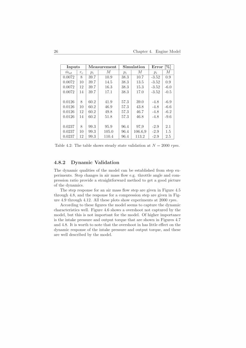
The measurements are performed under steady-state conditions, i.e.when all dynamic effects have died out. In order to keep down thenumber of measurements the test have been performed only at enginespeed 2000 rpm and at optimal ignition angle. This engine speed hasbeen chosen because is a very common engine speed during driving.The simulation results and measured data are presented in Table 4.2.Error stand for the errors made by the model. The errors are simplycalculated as
Error =Simulated value − Measured value
Measured value
To save space in the tables, the units for the quantities in the tablesdo not always follow the standard nomenclature in the report. Forconvenience all units which appear in the tables are listed her, air massflow [kg/s], pressure [kPa] and torque [Nm].
In Table 4.2 it can be seen that the error for both intake pressure andtorque are quit small. But it can be noted that the error in the outputtorque varies a lot with different air mass flows, this indicate that themodel of the combustion is not perfect. Another thing worth noting isthat the torque error is about the same for different compression ratios.This indicates that in spite of the problems with the combustion model,its seems to capture how the torque depends on the compression ratioquite well.
26 Chapter 4. Engine Model
Inputs Measurement Simulation Error [%]mat rc pi M pi M pi M
0.0072 8 39.7 10.9 38.3 10.7 -3.52 0.90.0072 10 39.7 14.5 38.3 13.5 -3.52 0.90.0072 12 39.7 16.3 38.3 15.3 -3.52 -6.00.0072 14 39.7 17.1 38.3 17.0 -3.52 -0.5
0.0126 8 60.2 41.9 57.3 39.0 -4.8 -6.90.0126 10 60.2 46.9 57.3 43.8 -4.8 -6.60.0126 12 60.2 49.8 57.3 46.7 -4.8 -6.20.0126 14 60.2 51.8 57.3 46.8 -4.8 -9.6
0.0237 8 99.3 95.9 96.4 97,9 -2.9 2.10.0237 10 99.3 105.0 96.4 106.6,9 -2.9 1.50.0237 12 99.3 110.4 96.4 113.2 -2.9 2.5
Table 4.2: The table shows steady state validation at N = 2000 rpm.
4.8.2 Dynamic Validation
The dynamic qualities of the model can be established from step ex-periments. Step changes in air mass flow e.g. throttle angle and com-pression ratio provide a straightforward method to get a good pictureof the dynamics.
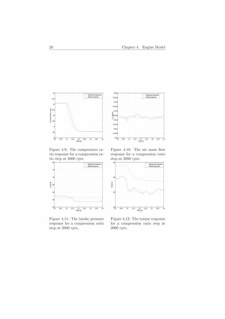
The step response for an air mass flow step are given in Figure 4.5through 4.8, and the response for a compression step are given in Fig-ure 4.9 through 4.12. All these plots show experiments at 2000 rpm.
According to these figures the model seems to capture the dynamiccharacteristics well. Figure 4.6 shows a overshoot not captured by themodel, but this is not important for the model. Of higher importanceis the intake pressure and output torque that are shown in Figures 4.7and 4.8. It is worth to note that the overshoot in has little effect on thedynamic response of the intake pressure and output torque, and theseare well described by the model.
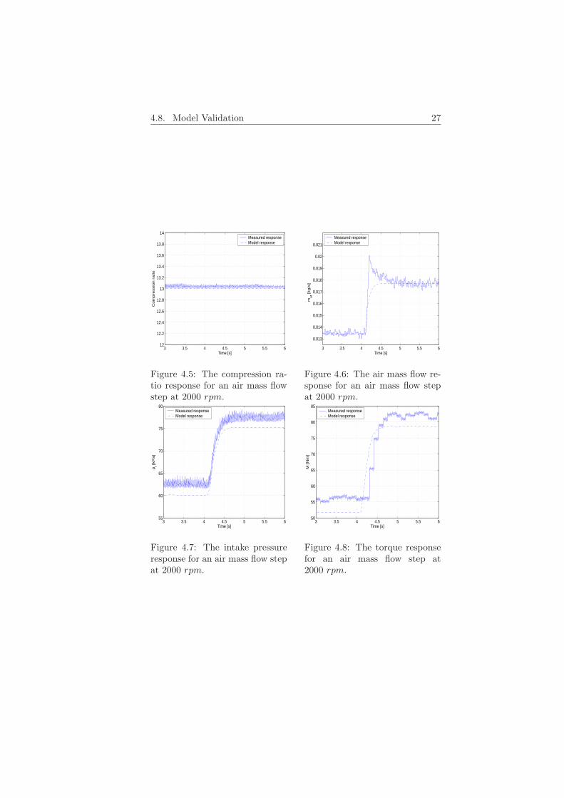
4.8. Model Validation 27
3 3.5 4 4.5 5 5.5 612
12.2
12.4
12.6
12.8
13
13.2
13.4
13.6
13.8
14
Time [s]
Co
mp
ressio
n r
atio
Measured responseModel response
Figure 4.5: The compression ra-tio response for an air mass flowstep at 2000 rpm.
3 3.5 4 4.5 5 5.5 6
0.013
0.014
0.015
0.016
0.017
0.018
0.019
0.02
0.021
Time [s]
ma
t [kg
/s]
Measured responseModel response
.
Figure 4.6: The air mass flow re-sponse for an air mass flow stepat 2000 rpm.
3 3.5 4 4.5 5 5.5 655
60
65
70
75
80
Time [s]
pi [
kP
a]
Measured responseModel response
Figure 4.7: The intake pressureresponse for an air mass flow stepat 2000 rpm.
3 3.5 4 4.5 5 5.5 650
55
60
65
70
75
80
85
Time [s]
M [N
m]
Measured responseModel response
Figure 4.8: The torque responsefor an air mass flow step at2000 rpm.
28 Chapter 4. Engine Model
10 10.5 11 11.5 12 12.5 13 13.5 148
8.5
9
9.5
10
10.5
11
11.5
12
Time [s]
Co
mp
ressio
n r
atio
Measured responseModel response
Figure 4.9: The compression ra-tio response for a compression ra-tio step at 2000 rpm.
10 10.5 11 11.5 12 12.5 13 13.5 140.01
0.0105
0.011
0.0115
0.012
0.0125
0.013
0.0135
0.014
0.0145
0.015
Time [s]
ma
t [kg
/s]
Measured responseModel response
.
Figure 4.10: The air mass flowresponse for a compression ratiostep at 2000 rpm.
10 10.5 11 11.5 12 12.5 13 13.5 1450
55
60
65
70
75
80
Time [s]
pi [
kP
a]
Measured responseModel response
Figure 4.11: The intake pressureresponse for a compression ratiostep at 2000 rpm.
10 10.5 11 11.5 12 12.5 13 13.5 1430
35
40
45
Time [s]
M [N
m]
Measured responseModel response
Figure 4.12: The torque responsefor a compression ratio step at2000 rpm.
Chapter 5
Preliminary Study
In order to decide the main structure of the controller it is importantto gain as much knowledge as possible about the system that is tobe controlled. The aim of this chapter is to gathering some of theinformation about the system that emerges during the model building.Two questions that are particular important to answer is:
• Which signals can be used as output signals from the controller?
• Which signals can be used as input signals to the controller?
There can also be very good to have a knowledge of importanttransfer functions such as the transfer function from air mass flow tooutput torque.
5.1 Controller Signals
Some of the signals that are interesting for torque control purposes isdiscussed bellow.
5.1.1 Air-Flow Past Throttle
Air flow past throttle (or actually throttle angle) is the signal whichthe driver normally uses to control the torque in a car and therefore anatural chose as output signal from the controller. The time constantfor the air flow past throttle to torque is around 0.50 s.
5.1.2 Ignition Angle
With the ignition angle its possible to control the torque much fasterthan with the air mass flow. The time constant for ignition angle
29
30 Chapter 5. Preliminary Study
to torque is in order of one engine cycle, and therefore instantaneousin our point of view. An alternative would be to use this signal asa complementary output signal. But drawbacks with this signal ishowever that it have a direct influence on the efficiency of the engine,which means that changing it from its optimal value can give the enginea poor fuel economy. Another thing that makes the ignition angleunsuitable for this purpose is that changing it from its optimal value canmake the engine start knocking, and knocking is extremely dangerousfor an engine. In addition to this the ignition angle can not be controlledwith the computer system used for controller implementation. For thesereasons the idea with the ignition angel as a complementary have beenrejected.
5.1.3 Compression Ratio
The compression ratio is controlled by the engine’s control system andcan in our case be seen as a measurable disturbance. An alternative canbe to feed forward the compression ratio to the controller. But sincethis will result in a more complex controller structure this alternativehas not been tested in this thesis.
In the previous chapter the time constant for compression ratio totorque was derived to 0.40 s.
5.1.4 Torque
The most natural choice when designing a controller for the torque is ofcourse to feed back the engines output torque, and let the error betweena set point torque and the output torque govern the controller. But ona production engine the output torque is not measured. Note that inthe engine lab there is possible to measure the torque. This meansthat to be able to use a feedback structure according to Figure 2.4 inChapter 2, an observer that can estimate the torque from measurablesignals have to be developed.
5.1.5 Summary
According to this investigation a control structure with the input signalsreference torque and estimated torque, and the output signal air massflow, would be the best choice.
The problem with only being able to use the air flow signal as outputsignal is that this signal is slower then the disturbance. This means thatthe effects of the disturbance never can be completely gone, but thereis reason to believe that this control structure can reduce the effect ofthe disturbance.
5.2. Transfer Function 31
5.2 Transfer Function
When developing a control algorithm it is good and sometimes neces-sary to know how the transfer function for different signals looks like.The most important transfer function in this thesis is the air mass flowto torque.
If the throttle saturation, throttle time delay and ignition angle isneglected in the model in Chapter 4, a model for fixed compressionratios can be described as
dmat
dt = − 1τthmat + 1
τthmatref
dpi
dt = RTi
Vimat − VdN/60s0
2Vipi − VdN/60s1
2Vi︸ ︷︷ ︸α
M =(κqhvVds02π15RTi2
(1 − 1
r(γ−1)c
)+ Vd
2πnr
)pi + κqhvVds1
2π15RTinr
(1 − 1
r(γ−1)c
)− Vdpe
2πnr−AN2 −BN − C
This is still a nonlinear system, and can not be described with atransfer function. But by neglecting α in the equations above a linearsystem that still capture most of the dynamics is received as
dmat
dt = − 1τthmat + 1
τthmatref
dpi
dt = RTi
Vimat − VdN/60s0
Vinrpi
M =(κqhvVds02π15RTi2
(1 − 1
r(γ−1)c
)+ Vd
2π2
)pi +
κqhvVds12π15RTi2
(1 − 1
r(γ−1)c
)︸ ︷︷ ︸
β
− Vdpe2π2︸ ︷︷ ︸δ
−AN2 −BN − C︸ ︷︷ ︸ψ
β, δ and ψ are only static displacements, therefore they can beneglected. The transfer function from air mass flow to torque can nowbe derived as
G(s) =RTi
Viτth
(κqhvVdS02π15RTi2
(1 − 1
rγ−1c
)+ Vd
2π2
)(s+ 1
τth
) (s+ VdN/60
Vi2
) (5.1)
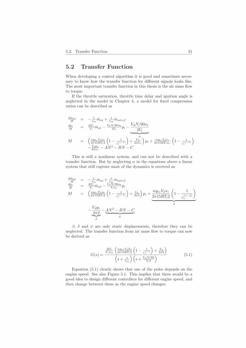
Equation (5.1) clearly shows that one of the poles depends on theengine speed. See also Figure 5.1. This implies that there would be agood idea to design different controllers for different engine speed, andthen change between these as the engine speed changes.
32 Chapter 5. Preliminary Study
−35 −30 −25 −20 −15 −10 −5 0−1
−0.8
−0.6
−0.4
−0.2
0
0.2
0.4
0.6
0.8
1
Real Axis
Imag
inar
y A
xis
Pole 1Pole 2
Figure 5.1: A plot that shows how one of the poles moves with differentengine speeds, that pole is marked with a circle and moves from right toleft along the real axis as the engine speed increases. The engine speedchanges from 1000 rpm to 4500 rpm. The other pole, independent ofoperating characteristics, is marked with a square.
Chapter 6
Control Algorithm
In this chapter the development and evaluation of the control algorithmis described. The work flow can be summarized as follows:
1. Design and Configuration. Determine a controller structure andits parameters. This work is done with help of computer simula-tions.
2. Implementation. When the controller performs well on the sim-ulated system it should be tested on the real system. To be ableto do this the selected controller must be implemented on the ac-tual system. The controller is implemented with help of SIMULINK
Real-Time Workshop with generates code to a real time platform.
3. Testing and Evaluation. The evaluation of the controller is thelast step. If the controller does not fulfill the demands the designermust restart at step 1.
The controller developed in this chapter is designed to work aroundengine speed, 2000 rpm. To get a controller that works over the entireengine operating range, the controller should be extended with gainscheduling that change parameters of the controller for different enginespeeds. But this has not been done in this thesis.
6.1 Control Demands
The main goal with the control design is of course to develop a con-troller that increases the driveability of a car that is equipped with avariable compression engine. A good driveability can be obtained if thecontroller is design so:
33
34 Chapter 6. Control Algorithm
• Torque changes due to changes in compression ratio are substan-tially reduced. In other words system disturbances shall havelittle influence on the output.
• The controlled variable is good at following the reference signal.
One problem is that these two demands stand in conflict with eachother [5], which means that if a controller is designed to follow thereference signal perfectly, its usually not so good at dealing with modelerrors and system disturbances. Therefore there is important here tofind a design that give a good compromise between these two demands.
6.2 Control Structure
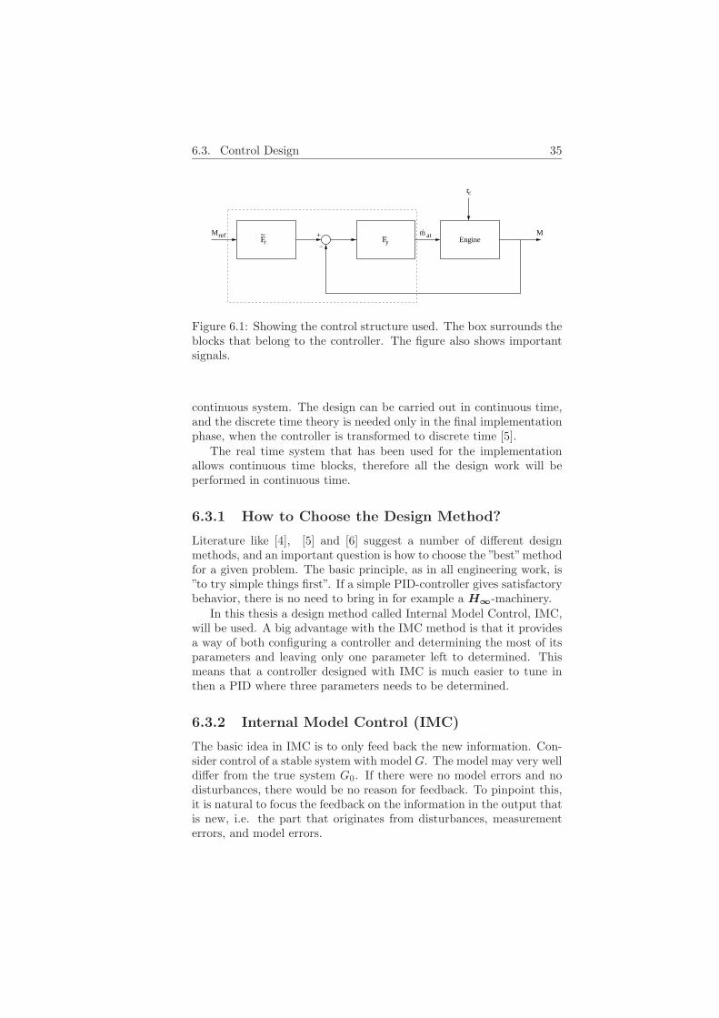
It is useful to treat the closed loop properties (i.e. sensitivity androbustness) separately from the servo properties (i.e. the transfer func-tion Gc from r to y). The key to this separation is that the sensitivityfunction S and complementary sensitivity function T depend only onFy, and not on Fr. A natural approach is thus to first choose Fy sothat S and T get the desired properties. If this does not give acceptableservo properties for closed loop system the filter Fr is modified. Thisfilter can be used to ”soften” fast changes in the reference signal. Frthen is of low pass character which means that the peak values of thecontroller input decrease.
This results in the controller structure in Figure 6.1. Note thatduring the design of the controller the torque signal is treated as ameasurable signal, and later it is replaced by the estimated torque.
Input signal is the error between engine torque and the referencetorque. Where the driver controls the reference torque. Output signalis the air flow past throttle. Worth noting is that this control structureinvolves a different way of control the torque. Normally the driveradjusts the torque with the air flow (or actually the throttle angle).But with this method the driver controls the torque with a torquereference signal.
6.3 Control Design
In modern control systems the controllers are almost exclusively dig-itally implemented in computers, signal processors or dedicated hard-ware. This means that the controller will operate in discrete time,while the controlled physical system naturally is described in continu-ous time. With today’s fast computers the sampling in the controllercan be chosen very fast, compare to the time constant of the controlledsystem. Then the controller approximately can be considered as a time
6.3. Control Design 35
mat.
+
−
Mref
rc
yFrF Engine~ M
Figure 6.1: Showing the control structure used. The box surrounds theblocks that belong to the controller. The figure also shows importantsignals.
continuous system. The design can be carried out in continuous time,and the discrete time theory is needed only in the final implementationphase, when the controller is transformed to discrete time [5].
The real time system that has been used for the implementationallows continuous time blocks, therefore all the design work will beperformed in continuous time.
6.3.1 How to Choose the Design Method?
Literature like [4], [5] and [6] suggest a number of different designmethods, and an important question is how to choose the ”best”methodfor a given problem. The basic principle, as in all engineering work, is”to try simple things first”. If a simple PID-controller gives satisfactorybehavior, there is no need to bring in for example a H∞-machinery.
In this thesis a design method called Internal Model Control, IMC,will be used. A big advantage with the IMC method is that it providesa way of both configuring a controller and determining the most of itsparameters and leaving only one parameter left to determined. Thismeans that a controller designed with IMC is much easier to tune inthen a PID where three parameters needs to be determined.
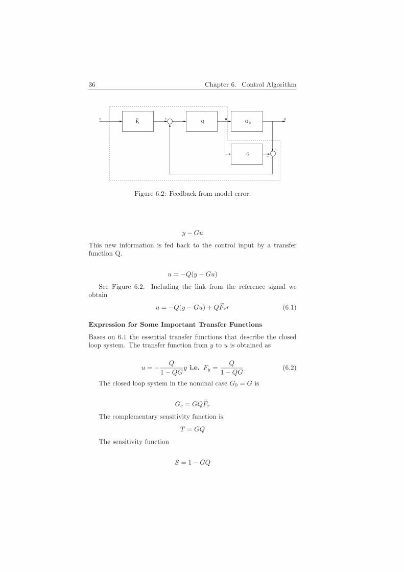
6.3.2 Internal Model Control (IMC)
The basic idea in IMC is to only feed back the new information. Con-sider control of a stable system with model G. The model may very welldiffer from the true system G0. If there were no model errors and nodisturbances, there would be no reason for feedback. To pinpoint this,it is natural to focus the feedback on the information in the output thatis new, i.e. the part that originates from disturbances, measurementerrors, and model errors.
36 Chapter 6. Control Algorithm
+
−rF
~G 0
+
−
Q
G
ur y
Figure 6.2: Feedback from model error.
y −Gu
This new information is fed back to the control input by a transferfunction Q.
u = −Q(y −Gu)
See Figure 6.2. Including the link from the reference signal weobtain
u = −Q(y −Gu) +QFrr (6.1)
Expression for Some Important Transfer Functions
Bases on 6.1 the essential transfer functions that describe the closedloop system. The transfer function from y to u is obtained as
u = − Q
1 −QGy i.e. Fy =
Q
1 −QG(6.2)
The closed loop system in the nominal case G0 = G is
Gc = GQFr
The complementary sensitivity function is
T = GQ
The sensitivity function
S = 1 −GQ
6.3. Control Design 37
Design Based on IMC
How to choose Q? The ideal choice Q = G−1, which would make S = 0and Gc = 1 is not possible since it corresponds to Fy = ∞, but is stillimportant guidance. What makes this choice impossible, and how canQ be modified to a possible and good choice:
1. G has more poles then zeros, and the inverse cannot be physicallyrealized. Use Q(s) = 1
(λs+1)nG−1(s) with n chosen so that Q(s)
can be realized (numerator ≤ denominator). λ is a design param-eter that can be adjusted to desired bandwidth of the closed loopsystem.
2. G has instable zero (it is non-minimum phase) which would becanceled when GG−1 is formed. This would given an unstableclosed loop system. There are two possibilities if G(s) has thefactor (−βs+ 1) in the numerator.
• Ignore (−βs+ 1) when Q is formed.
• Replace (−βs+1) with (βs+1) when Q is formed. This onlygives a phase error and no amplitude error in the model.
In both cases the original G is used when the controller is formedaccording to 6.2.
3. G has a time-delay, i.e. the factor e−sτ . There are two possibili-ties.
(a) Ignore e−sτ when Q is formed, but not in 6.2.
(b) Approximate e−sτ with 1−sτ/21+sτ/2 and use step 2. If necessary
use the same approximation of e−sτ in equation 6.2.
All the information and design rules for IMC can be found in [5].
6.3.3 Controller Calculations
In the previous section it was clear that in order to calculate a con-troller with IMC an internal model, G, in transfer from is needed. Insection 5.2 the model in chapter 4 is approximated with a transferfunction as
G(s) =RTi
Viτth
(κqhvVdS02π15RTinr
(1 − 1
rγ−1c
)+ Vd
2πnr
)(s+ 1
τth
) (s+ VdN/60
Vinr
) (6.3)
38 Chapter 6. Control Algorithm
With equation 6.3 as internal model, G, an IMC controller can becalculated according to the design rules in section 6.3.2.
Using equation 6.3 and values from Appendix B, the transfer func-tion G can be calculated at point rc = 11 and N = 2000 rpm. Where afix compression ratio can be chosen because changes in compression ra-tio results only in small dynamic changes in G. Engine speed, 2000 rpm,is the operating point which the controller is designed to work around.
G(s) =9.422 · 105
s2 + 26.67s+ 177.8(6.4)
If the time delay in throttle is taken into account transfer functionG looks like
G(s) =9.422 · 105
s2 + 26.67s+ 177.8e−0.4s
Suppose theG can be written asG(s) = G1(s)e−0.4s. Approach 3(a)for handling time delays implies that the time delay is ignore when Qis formed but not in 6.2.
G(s) has 2 more poles then zeroes, therefore according to rule 1Q(s) shall be chosen as
Q(s) =G(s)−1
(λs+ 1)2=s2 + 26.67s+ 177.89.422 · 105(λs+ 1)2
Using equation 6.2 and compensate for the time delay gives thecontroller
Fy(s) =Q(s)
1 −Q(s)G1(s)e−sτ
Let F 0y = Q/(1 − QG1) be the controller designed for the system
without time delays. Simple manipulations then give the controller
Fy =F 0y (s)
1 + (1 − e−sτ )F 0y (s)G1(s)
where G1 is
G1 =9.422 · 105
s2 + 26.67s+ 177.8
6.3. Control Design 39
+
−rF
~Mref mat.
−sL(e
+
+
M
yF0
−1) G 1
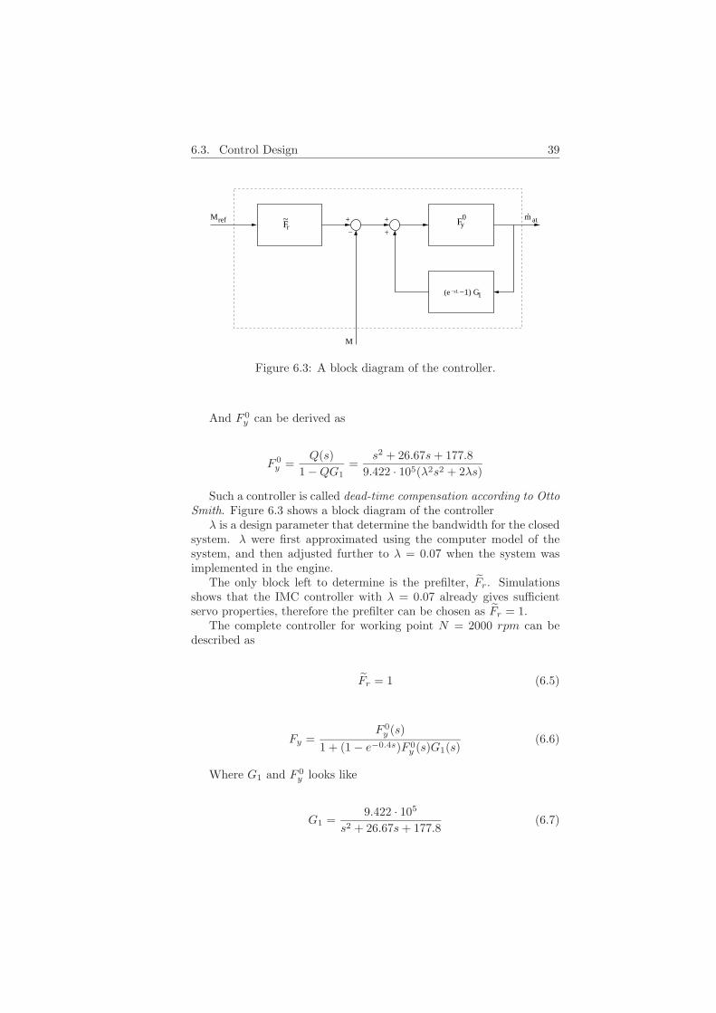
Figure 6.3: A block diagram of the controller.
And F 0y can be derived as
F 0y =
Q(s)1 −QG1
=s2 + 26.67s+ 177.8
9.422 · 105(λ2s2 + 2λs)
Such a controller is called dead-time compensation according to OttoSmith. Figure 6.3 shows a block diagram of the controller
λ is a design parameter that determine the bandwidth for the closedsystem. λ were first approximated using the computer model of thesystem, and then adjusted further to λ = 0.07 when the system wasimplemented in the engine.
The only block left to determine is the prefilter, Fr. Simulationsshows that the IMC controller with λ = 0.07 already gives sufficientservo properties, therefore the prefilter can be chosen as Fr = 1.
The complete controller for working point N = 2000 rpm can bedescribed as
Fr = 1 (6.5)
Fy =F 0y (s)
1 + (1 − e−0.4s)F 0y (s)G1(s)
(6.6)
Where G1 and F 0y looks like
G1 =9.422 · 105
s2 + 26.67s+ 177.8(6.7)
40 Chapter 6. Control Algorithm
F 0y =
s2 + 26.67s+ 177.84.616 · 103s2 + 1.319 · 105s
(6.8)
6.4 Observer
As the torque is not measurable the alternative is to estimate the torquefrom measurable signals. The observer is developed from the alreadyexisting torque model, by excluding the throttle dynamic and the com-pression ratio dynamic, since the sensors already measure the true dy-namic in this signals. Besides the throttle and compression ratio modelsalso the ignition angle map is excluded. In other words the observer isderived using equations (4.13), (4.14), (4.15), (4.17), (4.18), (4.19) and(4.20) from chapter 4. The observer can be derived as
dpi
dt = RTi
Vimat − VdN/60s0
Vinrpi
M =(κqhvVds02π15RTi2
(1 − 1
r(γ−1)c
)+ Vd
2π2
)pi + κqhvVds1
2π15RTi2
(1 − 1
r(γ−1)c
)−Vdpe
2π2 −AN2 −BN − C
The observer estimates the intake pressure, pi, and the torque, M ,from the measurable signals air mass flow, mat, intake manifold tem-perature, Ti, compression ratio, rc, and engine speed, N . It is worth tonote that the intake pressure actually is a measurable signal, but sincethe measured intake pressure is a very noisy signal, the observer insteadestimates the intake pressure from the air mass flow signal. The rest ofthe parameters are constants and can be found in Appendix B.
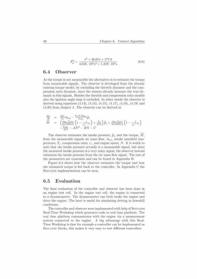
Figure 6.4 shows how the observer estimates the torque and howthe estimated torque is fed back to the controller. In Appendix C theSIMULINK implementation can be seen.
6.5 Evaluation
The final evaluation of the controller and observer has been done inan engine test cell. In the engine test cell, the engine is connectedto a dynamometer. The dynamometer can both brake the engine anddrive the engine. The later is useful for simulating driving in downhillconditions.
The controller and observer were implemented with help of SIMULINK
Real-Time Workshop which generates code to real time platform. Thereal time platform communicates with the engine via a measurementsystem connected to the engine. A big advantage with this Real-Time Workshop is that for example a controller can be implemented asSIMULINK blocks, this makes it very easy to test different controllers.
6.5. Evaluation 41
m at.
rc
m at. rc Ti
M
Mref
Engine
N
MController
Observer
Figure 6.4: The observer estimates the torque from measurable signalsand feedback the estimated torque to the controller.
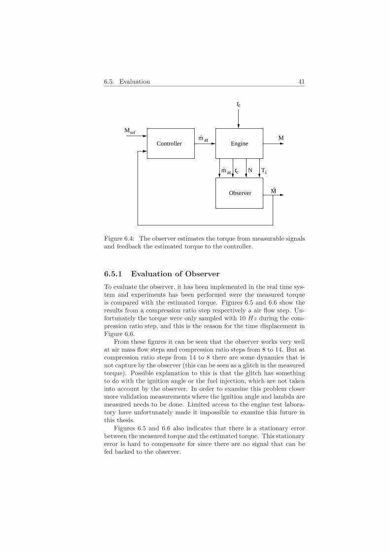
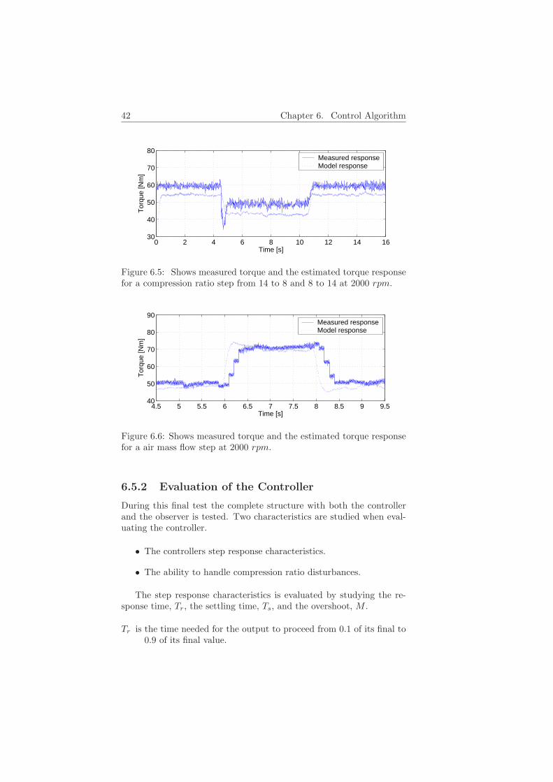
6.5.1 Evaluation of Observer
To evaluate the observer, it has been implemented in the real time sys-tem and experiments has been performed were the measured torqueis compared with the estimated torque. Figures 6.5 and 6.6 show theresults from a compression ratio step respectively a air flow step. Un-fortunately the torque were only sampled with 10 Hz during the com-pression ratio step, and this is the reason for the time displacement inFigure 6.6.
From these figures it can be seen that the observer works very wellat air mass flow steps and compression ratio steps from 8 to 14. But atcompression ratio steps from 14 to 8 there are some dynamics that isnot capture by the observer (this can be seen as a glitch in the measuredtorque). Possible explanation to this is that the glitch has somethingto do with the ignition angle or the fuel injection, which are not takeninto account by the observer. In order to examine this problem closermore validation measurements where the ignition angle and lambda aremeasured needs to be done. Limited access to the engine test labora-tory have unfortunately made it impossible to examine this future inthis thesis.
Figures 6.5 and 6.6 also indicates that there is a stationary errorbetween the measured torque and the estimated torque. This stationaryerror is hard to compensate for since there are no signal that can befed backed to the observer.
42 Chapter 6. Control Algorithm
0 2 4 6 8 10 12 14 1630
40
50
60
70
80
Time [s]
Tor
que
[Nm
]
Measured responseModel response
Figure 6.5: Shows measured torque and the estimated torque responsefor a compression ratio step from 14 to 8 and 8 to 14 at 2000 rpm.
4.5 5 5.5 6 6.5 7 7.5 8 8.5 9 9.540
50
60
70
80
90
Time [s]
Tor
que
[Nm
]
Measured responseModel response
Figure 6.6: Shows measured torque and the estimated torque responsefor a air mass flow step at 2000 rpm.
6.5.2 Evaluation of the Controller
During this final test the complete structure with both the controllerand the observer is tested. Two characteristics are studied when eval-uating the controller.
• The controllers step response characteristics.
• The ability to handle compression ratio disturbances.
The step response characteristics is evaluated by studying the re-sponse time, Tr, the settling time, Ts, and the overshoot, M .
Tr is the time needed for the output to proceed from 0.1 of its final to0.9 of its final value.
6.5. Evaluation 43
Ts is defined as the smallest time, t, which satisfies 1−p ≤ y(t) ≤ 1+pfor all t > Ts. y(t) is the output and p = 5%. In this case y(t)has the final value 1.
M is simply measurement of the overshoot in %.
All of these definitions can be found in [4]. The ability to handlecompression ratio disturbances is evaluated by studying M and Ts.Where Ts now is defined as the time from the start of the disturbanceuntil the output satisfies the 1−p ≤ y(t) ≤ 1+p for all t after the startof the disturbance.
Description of the Experiments
Two different experiments were made to validate the controller.
• Test 1 The controllers ability to handle compression ratiodisturbance are tested by changing rc from 8 to 14 and from 14to 8 at a constant output torque.
• Test 2 The step response characteristics are tested with atorque reference step from 60 Nm to 70 Nm and from 70 Nmto 60 Nm at both rc = 8 and rc = 14.
Results
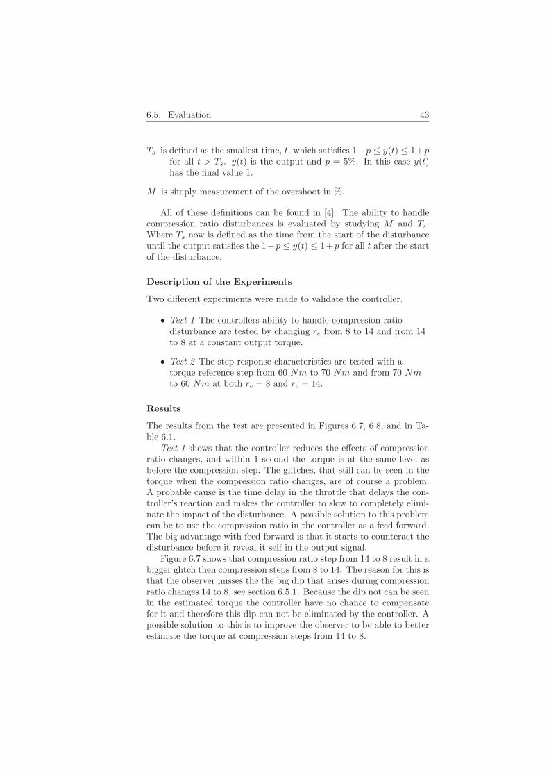
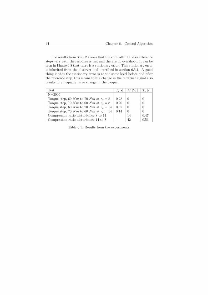
The results from the test are presented in Figures 6.7, 6.8, and in Ta-ble 6.1.
Test 1 shows that the controller reduces the effects of compressionratio changes, and within 1 second the torque is at the same level asbefore the compression step. The glitches, that still can be seen in thetorque when the compression ratio changes, are of course a problem.A probable cause is the time delay in the throttle that delays the con-troller’s reaction and makes the controller to slow to completely elimi-nate the impact of the disturbance. A possible solution to this problemcan be to use the compression ratio in the controller as a feed forward.The big advantage with feed forward is that it starts to counteract thedisturbance before it reveal it self in the output signal.
Figure 6.7 shows that compression ratio step from 14 to 8 result in abigger glitch then compression steps from 8 to 14. The reason for this isthat the observer misses the the big dip that arises during compressionratio changes 14 to 8, see section 6.5.1. Because the dip not can be seenin the estimated torque the controller have no chance to compensatefor it and therefore this dip can not be eliminated by the controller. Apossible solution to this is to improve the observer to be able to betterestimate the torque at compression steps from 14 to 8.
44 Chapter 6. Control Algorithm
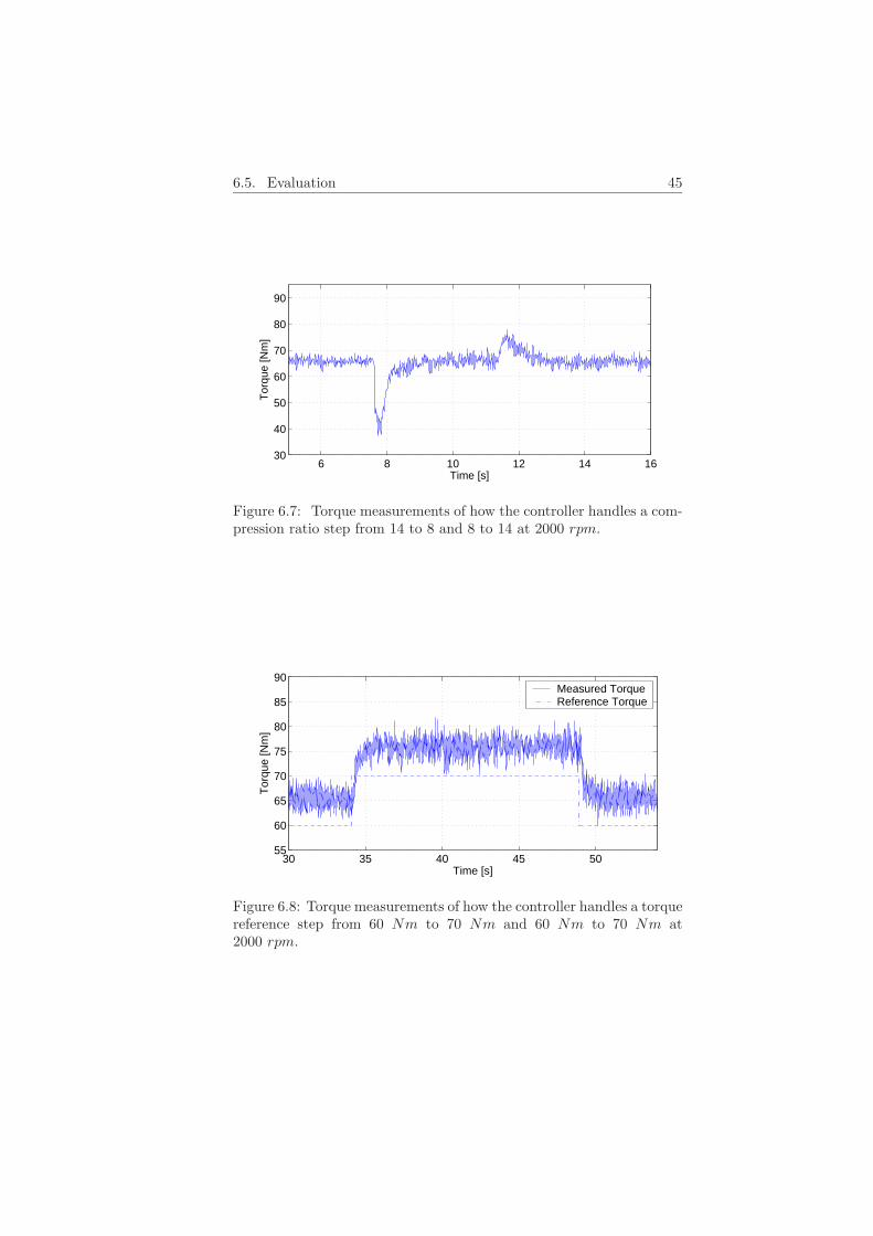
The results from Test 2 shows that the controller handles referencesteps very well, the response is fast and there is no overshoot. It can beseen in Figure 6.8 that there is a stationary error. This stationary erroris inherited from the observer and described in section 6.5.1. A goodthing is that the stationary error is at the same level before and afterthe reference step, this means that a change in the reference signal alsoresults in an equally large change in the torque.
Test Tr[s] M [% ] Ts [s]N=2000Torque step, 60 Nm to 70 Nm at rc = 8 0.28 0 0Torque step, 70 Nm to 60 Nm at rc = 8 0.20 0 0Torque step, 60 Nm to 70 Nm at rc = 14 0.37 0 0Torque step, 70 Nm to 60 Nm at rc = 14 0.14 0 0Compression ratio disturbance 8 to 14 - 14 0.47Compression ratio disturbance 14 to 8 - 42 0.56
Table 6.1: Results from the experiments.
6.5. Evaluation 45
6 8 10 12 14 1630
40
50
60
70
80
90
Time [s]
Tor
que
[Nm
]
Figure 6.7: Torque measurements of how the controller handles a com-pression ratio step from 14 to 8 and 8 to 14 at 2000 rpm.
30 35 40 45 5055
60
65
70
75
80
85
90
Time [s]
Tor
que
[Nm
]
Measured TorqueReference Torque
Figure 6.8: Torque measurements of how the controller handles a torquereference step from 60 Nm to 70 Nm and 60 Nm to 70 Nm at2000 rpm.

46
Chapter 7
Conclusions and FutureWork
This chapter consists of a summary of the work done during this the-sis together with a restatement of the conclusions and a discussion ofpossible further work.
7.1 Summary
The aim with this thesis project has been to first develop a simplesimulation model which can be used for control design, and then developand test a torque control strategy. The work done during this thesiscan roughly be dived into 5 steps.
1. Gathering knowledge. The first step, when designing a controlstrategy was to gain as much knowledge as possible about the sys-tem that is to be controlled. The quality of the control structureis greatly dependent on the designer’s experience and knowledgeof the system. In order to obtain this a lot of documentationabout SI-engines have been gathered and studied.
2. Construct a model of the system. In order to efficiently controlthe system its preferable to have a system model that can beused for simulations. An MVEM that includes information abouttypical disturbances and reference signals was developed with helpof physical modeling.
3. Designing the control system. The design of the control systemstarts with deciding a main structure of the controller. Whena suitable control structure have been chosen the design of thecontrollers it self can commence.
47
48 Chapter 7. Conclusions and Future Work
4. Implementation of the controller When the controller performswell on the simulated system it should be tested on the real sys-tem. To be able to do this the controller must be implementedon the actual system. The controller is implemented with helpof SIMULINK Real-Time Workshop which generates code to a realtime platform.
5. Evaluation of the controller performance. The last step was totest and evaluate the controller. This has been done with help ofreal measurements in a engine test cell.
7.2 Accomplishments and Conclusion
The modeling of the torque was an important part of this thesis andmuch effort was put into learning how the system behaved. It wasfound that the system is very complex and has many dependencies.The model that was developed worked well and was as accurate as onecan expect given the simplifications made. The model proved to be agreat help in the design work.
Because the torque not is a measurable signal in a ordinary engine,an observer that could estimate the torque from measurable signalswas developed. The observer was developed from the already existingtorque model, by excluding the throttle- and the compression ratiodynamics, since the sensors already measure the ”true” dynamic in thissignals. The observer was proved to work better at compression stepsfrom 8 to 14 than 14 to 8, were a big dip at the output torque arises.In addition to this the lack of feedback in the observer made so therewas a static error at estimated torque.
The controller it self was designed using IMC. A big advantage withthe IMC method was that its both designs a controller and determinemost of its parameters leaving only one parameter left to determine.Witch makes it very easy to adjust the controller. The controller wasproved to reduce the effects from compression ratio changes. But aproblem is that the problems with the observer propagates to the con-troller. Its also reason to believed that a feed forward form the desiredcompression could make the controller performance even better.
7.3 Future Work
Possible future work with the model and the control algorithm are
• In order to further develop and test new control strategies themodel should be extended with models of the supercharger andthe intercooler.
7.3. Future Work 49
• The controller should be extended with a feed forward from thedesired compression ratio.
• More work need to be put down to get the observer work better.This is really important since the controller performance is highlydependent on the observer performance.
• The controller should be designed and tested for different enginespeeds.
• More experimental validations of the observer and the controllerneeds to be done.

50
References
[1] J. Heywood. Internal Combustion Engine Fundamentals. McGraw-Hill, 1988.
[2] L. Eriksson L. Nielsen. Vehicular Systems. Linkoping, Sweden,2001. Course material, Linkopings Universitet, Sweden.
[3] L. Ljung T. Glad. Modellbygge och simulering. Studentlitteratur,Lund, Sweden, 1991. In Swedish.
[4] L. Ljung T. Glad. Reglerteknik. Grundlaggande teori. Studentlit-teratur, Lund, Sweden, 2nd edition, 1989. In Swedish.
[5] L. Ljung T. Glad. Reglerteori. Flervariabla och olinjara metoder.Studentlitteratur, Lund, Sweden, 1997. In Swedish.
[6] T McKelvey A Stenman T. Glad, L. Ljung. Digital styrningkurskompendium. Linkoping, Sweden, 2000. Course material,Linkopings Universitet, Sweden.
[7] SAAB. New unique engine concept for high preformence and lowerfuel consumption. http://media.gm.com, February 2000.
[8] S. Sorenson E. Hendricks. Mean Value Modelling of Spark IgnitionEngines. SAE Paper 900616. SAE, 1990.
[9] Elbert Hendricks, Alain Chevalier, Michael Jensen, and Spencer C.Sorenson. Modelling of the Intake Manifold Filling Dynamics. SAEPaper 960037. SAE, 1996. SAE 960037.
51

52
Appendix A
Ignition AngleMeasurements
Below plots of how the output torque depends on the ignition angleand compression ratio is shown.
1520
2530
8
10
12
1425
30
35
40
45
θign
rc
Tor
que
Figure A.1: Measurements of torque as a function of compression ratioand ignition angle, at working point 40 Nm and 2000 rpm
53
54 Appendix A. Ignition Angle Measurements
1015
2025
8
10
12
1445
50
55
60
65
θign
rc
Tor
que
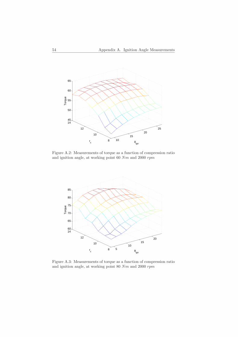
Figure A.2: Measurements of torque as a function of compression ratioand ignition angle, at working point 60 Nm and 2000 rpm
510
1520
8
10
12
1460
65
70
75
80
85
θign
rc
Tor
que
Figure A.3: Measurements of torque as a function of compression ratioand ignition angle, at working point 80 Nm and 2000 rpm
Appendix B
Model Parameters
Symbol value unitA 1.454 · 10−6 -B −3.599 · 10−3 -C 1.6262 · 101 -γ 1.3 -κ 0.74 -nr 2 -pe 1 · 105 Paqhv 44.3 · 106 J/kgR 287 J/(kg ·K)s0 0.91342 -s1 −11649 -Ti 300 Kτrc 0.40 -τth 0.075 -Vd 0.0016 m3
Vi 0.002 m3
Table B.1: The model parameters
55

56
Appendix C
SIMULINKImplementation
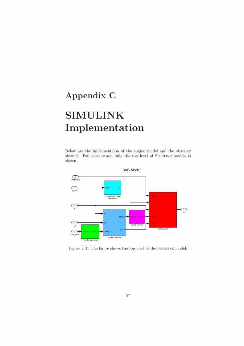
Below are the implementaion of the engine model and the observershowed. For convenience, only the top level of SIMULINK models isshown.
SVC Model
1
M
r_cref r_c
compression ratiodynamics
dotm_atref dotm_at
Throttle dynamics
N
T_i
dotm_at
dotm_ac
P_man
Intake manifold
dotm_ac dotm_f
Fuel injection
theta_ign
r_c
N
dotm_f
P_man
M
Combustion5
dotm_atref
4
T_i
3
N
2
r_cref
1
theta_ign
Figure C.1: The figure shows the top level of the SIMULINK model.
57
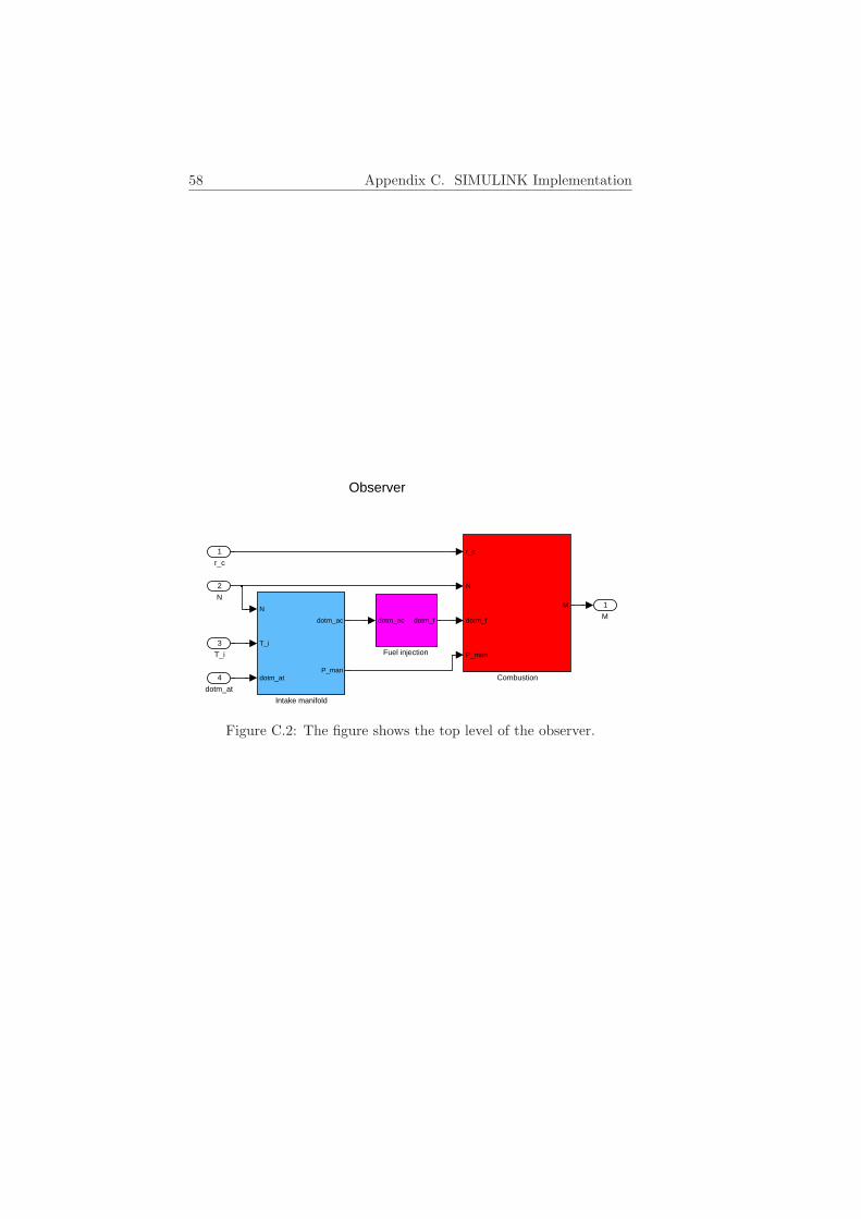
58 Appendix C. SIMULINK Implementation
Observer
1
MN
T_i
dotm_at
dotm_ac
P_man
Intake manifold
dotm_ac dotm_f
Fuel injection
r_c
N
dotm_f
P_man
M
Combustion4
dotm_at
3
T_i
2
N
1
r_c
Figure C.2: The figure shows the top level of the observer.