Embed Size (px)
DESCRIPTION
rmn
Citation preview

Copyright (C) 2005 by Bruker BioSpin GmbHAll rights reserved. No part of this publication may be reproduced, stored in a retrieval sys-tem, or transmitted, in any form, or by any means without the prior consent of the publisher.
Part Number H9469SA1 V2/April 13th 2005
Product names used are trademarks or registered trademarks of their respective holders.
TOPSPIN
Users Guide
DONE
INDEX
INDEX
Bruker software support is available via phone, fax, e-mail, Internet, or ISDN.Please contact your local office, or directly:
Address: Bruker BioSpin GmbHSoftware DepartmentSilberstreifenD-76287 RheinstettenGermany
Phone: +49 (721) 5161 455Fax: +49 (721) 5161 943E-mail: [email protected]: ftp.bruker.de / ftp.bruker.comWWW: www.bruker-biospin.de / www.bruker-biospin.com

3
Chapter 1 Getting Started . . . . . . . . . . . . . . . . . . . . . . . . . . . . . . . . . . . . . . . . . . 151.1 Document Conventions . . . . . . . . . . . . . . . . . . . . . . . . . . . . . . . . . . . . . . 15
Font Conventions . . . . . . . . . . . . . . . . . . . . . . . . . . . . . . . . . . . . . . . . . . 15File/directory Conventions . . . . . . . . . . . . . . . . . . . . . . . . . . . . . . . . . . . 15User Action Conventions . . . . . . . . . . . . . . . . . . . . . . . . . . . . . . . . . . . . 15
1.2 TOPSPIN Overview . . . . . . . . . . . . . . . . . . . . . . . . . . . . . . . . . . . . . . . . . . 16Functionality . . . . . . . . . . . . . . . . . . . . . . . . . . . . . . . . . . . . . . . . . . . . . . 16Available Documentation . . . . . . . . . . . . . . . . . . . . . . . . . . . . . . . . . . . . 17
1.3 TOPSPIN license . . . . . . . . . . . . . . . . . . . . . . . . . . . . . . . . . . . . . . . . . . . . 171.4 Startup TOPSPIN . . . . . . . . . . . . . . . . . . . . . . . . . . . . . . . . . . . . . . . . . . . . 181.5 Configuration . . . . . . . . . . . . . . . . . . . . . . . . . . . . . . . . . . . . . . . . . . . . . . 181.6 How to Display Spectra . . . . . . . . . . . . . . . . . . . . . . . . . . . . . . . . . . . . . . 19
How to Open Data from the Menu . . . . . . . . . . . . . . . . . . . . . . . . . . . . . 19How to Open Data from the Browser . . . . . . . . . . . . . . . . . . . . . . . . . . . 20How to Define Alias Names for Data . . . . . . . . . . . . . . . . . . . . . . . . . . . 20How to Open Data in Other Ways . . . . . . . . . . . . . . . . . . . . . . . . . . . . . 20
1.7 How to Display Peaks, Integrals, ... together with the Spectrum . . . . . . 201.8 How to Display Projections/1D Spectra with 2D Spectra . . . . . . . . . . . . 211.9 How to Superimpose Spectra in Multiple Display . . . . . . . . . . . . . . . . . 211.10 How to Print or Export the Contents of a Data Window . . . . . . . . . . . . . 22
How to Print Data . . . . . . . . . . . . . . . . . . . . . . . . . . . . . . . . . . . . . . . . . . 22How to Copy a Data Window to Clipboard . . . . . . . . . . . . . . . . . . . . . . 22How to Store (Export) a Data Window as Graphics File . . . . . . . . . . . . 22
1.11 How to Process Data . . . . . . . . . . . . . . . . . . . . . . . . . . . . . . . . . . . . . . . . 221.12 How to Archive Data . . . . . . . . . . . . . . . . . . . . . . . . . . . . . . . . . . . . . . . . 231.13 How to Import NMR Data Stored in Special Formats. . . . . . . . . . . . . . . 241.14 How to Fit Peaks and Deconvolve Overlapping Peaks . . . . . . . . . . . . . . 241.15 How to Compute Fids by Simulating Experiments . . . . . . . . . . . . . . . . . 241.16 How to Add Your Own Functionalities . . . . . . . . . . . . . . . . . . . . . . . . . . 25
How to Create Macros . . . . . . . . . . . . . . . . . . . . . . . . . . . . . . . . . . . . . . 25How to Create AU (automation) Programs . . . . . . . . . . . . . . . . . . . . . . 25How to Create Python Programs . . . . . . . . . . . . . . . . . . . . . . . . . . . . . . . 26
1.17 How to Automate Data Acquisition. . . . . . . . . . . . . . . . . . . . . . . . . . . . . 26Chapter 2 The TOPSPIN Interface . . . . . . . . . . . . . . . . . . . . . . . . . . . . . . . . . . . . . 27
2.1 The Topspin Window. . . . . . . . . . . . . . . . . . . . . . . . . . . . . . . . . . . . . . . . 27How to Use Multiple Data Windows . . . . . . . . . . . . . . . . . . . . . . . . . . . 28How to Use the Title bar . . . . . . . . . . . . . . . . . . . . . . . . . . . . . . . . . . . . . 29How to Use the Menu bar . . . . . . . . . . . . . . . . . . . . . . . . . . . . . . . . . . . . 29How to Use the Upper Toolbar . . . . . . . . . . . . . . . . . . . . . . . . . . . . . . . . 30How to Use the Lower Toolbar . . . . . . . . . . . . . . . . . . . . . . . . . . . . . . . 31
2.2 Command Line Usage . . . . . . . . . . . . . . . . . . . . . . . . . . . . . . . . . . . . . . . 33
4
DONE
INDEX
INDEX
How to Put the Focus in the Command Line . . . . . . . . . . . . . . . . . . . . . 33How to Retrieve Previously Entered Commands . . . . . . . . . . . . . . . . . . 33How to Change Previously Entered Commands . . . . . . . . . . . . . . . . . . . 33How to Enter a Series of Commands . . . . . . . . . . . . . . . . . . . . . . . . . . . 34
2.3 Command Line History . . . . . . . . . . . . . . . . . . . . . . . . . . . . . . . . . . . . . . 342.4 Starting TOPSPIN commands from a Command Prompt . . . . . . . . . . . . . 352.5 Function Keys and Control Keys . . . . . . . . . . . . . . . . . . . . . . . . . . . . . . . 362.6 Help in Topspin . . . . . . . . . . . . . . . . . . . . . . . . . . . . . . . . . . . . . . . . . . . . 39
How to Open Online Help documents . . . . . . . . . . . . . . . . . . . . . . . . . . 39How to Get Tooltips . . . . . . . . . . . . . . . . . . . . . . . . . . . . . . . . . . . . . . . . 39How to Get Help on Individual Commands . . . . . . . . . . . . . . . . . . . . . . 40How to Use the Command Index . . . . . . . . . . . . . . . . . . . . . . . . . . . . . . 40
2.7 User Defined Functions Keys . . . . . . . . . . . . . . . . . . . . . . . . . . . . . . . . . 412.8 How to Open Multiple TOPSPIN Interfaces . . . . . . . . . . . . . . . . . . . . . . . 41
Chapter 3 Trouble Shooting . . . . . . . . . . . . . . . . . . . . . . . . . . . . . . . . . . . . . . . . . 433.1 General Tips and Tricks . . . . . . . . . . . . . . . . . . . . . . . . . . . . . . . . . . . . . . 433.2 History, Log Files, Stack Trace . . . . . . . . . . . . . . . . . . . . . . . . . . . . . . . . 433.3 How to Show or Kill TOPSPIN processes . . . . . . . . . . . . . . . . . . . . . . . . . 473.4 What to do if TOPSPIN hangs . . . . . . . . . . . . . . . . . . . . . . . . . . . . . . . . . . 473.5 How to Restart User Interface during Acquisition . . . . . . . . . . . . . . . . . 48
Chapter 4 Dataset Handling . . . . . . . . . . . . . . . . . . . . . . . . . . . . . . . . . . . . . . . . . 494.1 The Topspin Browser and Portfolio . . . . . . . . . . . . . . . . . . . . . . . . . . . . . 49
How to Open the Browser/Portfolio . . . . . . . . . . . . . . . . . . . . . . . . . . . . 51How to Open the Browser/Portfolio in a separate window . . . . . . . . . . 51How to Put the Focus in the Browser/Portfolio . . . . . . . . . . . . . . . . . . . 51How to Select Folders in the Browser . . . . . . . . . . . . . . . . . . . . . . . . . . 51How to Expand/Collapse a Folder in the Browser . . . . . . . . . . . . . . . . . 52How to Expand a Folder showing Pulse program and Title . . . . . . . . . . 52How to Add/Remove a Top Level Data Directory . . . . . . . . . . . . . . . . . 53How to Open a New Portfolio . . . . . . . . . . . . . . . . . . . . . . . . . . . . . . . . 53How to Save the current Portfolio . . . . . . . . . . . . . . . . . . . . . . . . . . . . . 54How to Remove Datasets from the Portfolio . . . . . . . . . . . . . . . . . . . . . 54How to Find Data and Add them to the Portfolio . . . . . . . . . . . . . . . . . . 54How to Sort Data in the Portfolio . . . . . . . . . . . . . . . . . . . . . . . . . . . . . . 54How to Add, Remove or Interpret Alias Names . . . . . . . . . . . . . . . . . . . 55
4.2 Creating Data . . . . . . . . . . . . . . . . . . . . . . . . . . . . . . . . . . . . . . . . . . . . . . 56How to Create a New Dataset . . . . . . . . . . . . . . . . . . . . . . . . . . . . . . . . . 56
4.3 Opening Data . . . . . . . . . . . . . . . . . . . . . . . . . . . . . . . . . . . . . . . . . . . . . . 57How to Open Data Windows Cascaded . . . . . . . . . . . . . . . . . . . . . . . . . 58How to Open Data from the Browser . . . . . . . . . . . . . . . . . . . . . . . . . . . 59How to Open Data from the Portfolio . . . . . . . . . . . . . . . . . . . . . . . . . . . 60

5
DONE
INDEX
INDEX
How to Automatically Select the first expno/procno of a dataset . . . . . 60How to Open Data from the Topspin menu . . . . . . . . . . . . . . . . . . . . . . 61How to Open Data from the Explorer, Konqueror or Nautilus . . . . . . . . 63How to Open Data from the Command Line . . . . . . . . . . . . . . . . . . . . . 64How to Open Special Format Data . . . . . . . . . . . . . . . . . . . . . . . . . . . . . 65How to Open a ZIP or JCAMP-DX file from the Windows Explorer . . 66
4.4 Saving/Copying Data . . . . . . . . . . . . . . . . . . . . . . . . . . . . . . . . . . . . . . . . 66How to Save or Copy Data . . . . . . . . . . . . . . . . . . . . . . . . . . . . . . . . . . . 66How to Save an Entire Dataset . . . . . . . . . . . . . . . . . . . . . . . . . . . . . . . . 67How to Save Processed Data . . . . . . . . . . . . . . . . . . . . . . . . . . . . . . . . . 68How to Save Acquisition Data . . . . . . . . . . . . . . . . . . . . . . . . . . . . . . . . 68How to Save Processed Data as Pseudo Raw Data . . . . . . . . . . . . . . . . . 68
4.5 Deleting Data . . . . . . . . . . . . . . . . . . . . . . . . . . . . . . . . . . . . . . . . . . . . . . 68How to Delete a Specific Dataset . . . . . . . . . . . . . . . . . . . . . . . . . . . . . . 68How to Delete Types of Datasets . . . . . . . . . . . . . . . . . . . . . . . . . . . . . . 69
4.6 Searching/Finding Data . . . . . . . . . . . . . . . . . . . . . . . . . . . . . . . . . . . . . . 71How to Find Data . . . . . . . . . . . . . . . . . . . . . . . . . . . . . . . . . . . . . . . . . . 71How to Display one of the Found Datasets . . . . . . . . . . . . . . . . . . . . . . 73How to Select Data from the Found Datasets . . . . . . . . . . . . . . . . . . . . . 73How to Add Selected Datasets to the Portfolio . . . . . . . . . . . . . . . . . . . 74How to Save Selected Datasets to a List . . . . . . . . . . . . . . . . . . . . . . . . . 74
4.7 Handling Data Files . . . . . . . . . . . . . . . . . . . . . . . . . . . . . . . . . . . . . . . . . 74How to List/Open the Current Dataset Files . . . . . . . . . . . . . . . . . . . . . . 74How to List/Open the current Dataset Files in the Windows Explorer . 75
4.8 Data Consistency Check . . . . . . . . . . . . . . . . . . . . . . . . . . . . . . . . . . . . . 76Chapter 5 Parameter Handling . . . . . . . . . . . . . . . . . . . . . . . . . . . . . . . . . . . . . . 79
5.1 Processing Parameters . . . . . . . . . . . . . . . . . . . . . . . . . . . . . . . . . . . . . . . 79How to Set a Processing Parameter from the Command Line . . . . . . . . 79How to Set Processing Parameters from the Parameter Editor . . . . . . . . 80How to Undo the Last Processing Parameter Change . . . . . . . . . . . . . . 81How to Display Processing Status Parameters . . . . . . . . . . . . . . . . . . . . 81How to Change Processed Data Dimensionality . . . . . . . . . . . . . . . . . . 81
5.2 Acquisition Parameters . . . . . . . . . . . . . . . . . . . . . . . . . . . . . . . . . . . . . . 82How to Set Acquisition Parameters . . . . . . . . . . . . . . . . . . . . . . . . . . . . 82How to Set an Acquisition Parameter from the Command Line . . . . . . 82How to Set Acquisition Parameters from the Parameter Editor . . . . . . . 83How to Undo the Last Acquisition Parameter Change . . . . . . . . . . . . . . 84How to Set Pulse Program Parameters . . . . . . . . . . . . . . . . . . . . . . . . . . 84How to Display Acquisition Status Parameters . . . . . . . . . . . . . . . . . . . 84How to Get Probehead/Solvent dependent Parameters . . . . . . . . . . . . . 84How to Change Acquisition Data Dimensionality . . . . . . . . . . . . . . . . . 84

6
DONE
INDEX
INDEX
How to Set Lock Parameters . . . . . . . . . . . . . . . . . . . . . . . . . . . . . . . . . . 85How to Set Routing Parameters . . . . . . . . . . . . . . . . . . . . . . . . . . . . . . . 85
Chapter 6 Data Processing . . . . . . . . . . . . . . . . . . . . . . . . . . . . . . . . . . . . . . . . . . 876.1 Interactive Processing . . . . . . . . . . . . . . . . . . . . . . . . . . . . . . . . . . . . . . . 87
How to Process Data with Single Commands . . . . . . . . . . . . . . . . . . . . 87How to Process data with Composite Commands . . . . . . . . . . . . . . . . . 88
6.2 Semi-automatic Processing . . . . . . . . . . . . . . . . . . . . . . . . . . . . . . . . . . . 88How to Use the Processing Guide in Automatic mode . . . . . . . . . . . . . . 88How to Use the Processing Guide in Interactive mode . . . . . . . . . . . . . 90
6.3 Processing Data with AU programs. . . . . . . . . . . . . . . . . . . . . . . . . . . . . 906.4 Serial Processing using Python programs . . . . . . . . . . . . . . . . . . . . . . . . 91
Chapter 7 Printing/Exporting Data . . . . . . . . . . . . . . . . . . . . . . . . . . . . . . . . . . . 957.1 Printing/plotting Data. . . . . . . . . . . . . . . . . . . . . . . . . . . . . . . . . . . . . . . . 95
How to Print/Plot from the Menu . . . . . . . . . . . . . . . . . . . . . . . . . . . . . . 95How to Plot Data from the Processing guide . . . . . . . . . . . . . . . . . . . . . 97How to Plot Data with the Plot Editor . . . . . . . . . . . . . . . . . . . . . . . . . . 97How to Print the Integral list . . . . . . . . . . . . . . . . . . . . . . . . . . . . . . . . . . 97How to Print the Peak list . . . . . . . . . . . . . . . . . . . . . . . . . . . . . . . . . . . . 98
7.2 Exporting Data . . . . . . . . . . . . . . . . . . . . . . . . . . . . . . . . . . . . . . . . . . . . . 99How to Copy data to Other Applications . . . . . . . . . . . . . . . . . . . . . . . . 99How to Store (Export) a Data Window as Graphics File . . . . . . . . . . . . 99
Chapter 8 1D Display . . . . . . . . . . . . . . . . . . . . . . . . . . . . . . . . . . . . . . . . . . . . . 1018.1 The 1D Data Window . . . . . . . . . . . . . . . . . . . . . . . . . . . . . . . . . . . . . . 1018.2 Displaying one Dataset in Multiple windows . . . . . . . . . . . . . . . . . . . . 102
How to Reopen a Dataset in a Second/Third etc. Window . . . . . . . . . . 102How to Rescale or Shift one Dataset in Multiple windows . . . . . . . . . 103
8.3 Changing the Display of a 1D Spectrum or FID . . . . . . . . . . . . . . . . . . 104How to Change the Vertical Scaling of the FID or Spectrum . . . . . . . 104How to Change the Horizontal Scaling of the FID or Spectrum . . . . . 104How to Shift a Spectral Region to the Left or to the Right . . . . . . . . . . 105How to Shift the Spectrum Up or Down . . . . . . . . . . . . . . . . . . . . . . . . 106
8.4 Using the Tab bar . . . . . . . . . . . . . . . . . . . . . . . . . . . . . . . . . . . . . . . . . . 106How to Display the Spectrum . . . . . . . . . . . . . . . . . . . . . . . . . . . . . . . . 107How to Set Processing Parameters . . . . . . . . . . . . . . . . . . . . . . . . . . . . 107How to Set Acquisition Parameters . . . . . . . . . . . . . . . . . . . . . . . . . . . 108How to Edit the Title . . . . . . . . . . . . . . . . . . . . . . . . . . . . . . . . . . . . . . . 109How to Edit the Pulse Program . . . . . . . . . . . . . . . . . . . . . . . . . . . . . . . 109How to Display the Peak list . . . . . . . . . . . . . . . . . . . . . . . . . . . . . . . . . 110How to Display the Integral list . . . . . . . . . . . . . . . . . . . . . . . . . . . . . . 115How to view Sample Information . . . . . . . . . . . . . . . . . . . . . . . . . . . . . 121How to Open the Jmol Molecule Structure Viewer . . . . . . . . . . . . . . . 122
7
DONE
INDEX
INDEX
How to Display the FID . . . . . . . . . . . . . . . . . . . . . . . . . . . . . . . . . . . . 1248.5 1D Display Options . . . . . . . . . . . . . . . . . . . . . . . . . . . . . . . . . . . . . . . . 124
How to Toggle between Hertz and ppm Axis Units . . . . . . . . . . . . . . . 124How to Switch on/off the Spectrum Overview display . . . . . . . . . . . . 124How to Switch Y-axis Display . . . . . . . . . . . . . . . . . . . . . . . . . . . . . . . 125
8.6 Show Display Properties/Regions/Files. . . . . . . . . . . . . . . . . . . . . . . . . 126How to Superimpose the Cursor Information . . . . . . . . . . . . . . . . . . . . 127How to Superimpose the Title on the Spectrum . . . . . . . . . . . . . . . . . . 127How to Superimpose the main Status Parameters on the Spectrum . . 127How to Superimpose the Integral Trails/Labels on the Spectrum . . . . 127How to Superimpose Peak Labels on the Spectrum . . . . . . . . . . . . . . . 127How to Show Individual Data Points of the Spectrum . . . . . . . . . . . . . 127How to Display the Main Dataset Properties . . . . . . . . . . . . . . . . . . . . 128How to Display a List of Files of a Dataset . . . . . . . . . . . . . . . . . . . . . 128
8.7 Saving Display Region . . . . . . . . . . . . . . . . . . . . . . . . . . . . . . . . . . . . . 130How to Save the Display Region for Re-display . . . . . . . . . . . . . . . . . 131How to Save the Display Region for Baseline or Phase Correction . . . 131How to Save the Display Region for Strip FT . . . . . . . . . . . . . . . . . . . 131
Chapter 9 2D Display . . . . . . . . . . . . . . . . . . . . . . . . . . . . . . . . . . . . . . . . . . . . . 1339.1 The 2D Data Window . . . . . . . . . . . . . . . . . . . . . . . . . . . . . . . . . . . . . . 1339.2 Changing the Display of a 2D spectrum . . . . . . . . . . . . . . . . . . . . . . . . 134
How to Change the Intensity Scaling . . . . . . . . . . . . . . . . . . . . . . . . . . 134How to Switch on/off Square 2D layout . . . . . . . . . . . . . . . . . . . . . . . . 135How to Zoom a 2D spectrum in/out . . . . . . . . . . . . . . . . . . . . . . . . . . . 136How to Shift a Spectral Region in the F2 direction (left/right) . . . . . . 137How to Shift a Spectral Region in the F1 direction (up/down) . . . . . . 137
9.3 Show Display Properties/Regions/Files. . . . . . . . . . . . . . . . . . . . . . . . . 1389.4 Using the Tab bar . . . . . . . . . . . . . . . . . . . . . . . . . . . . . . . . . . . . . . . . . . 139
How to Set Processing Parameters . . . . . . . . . . . . . . . . . . . . . . . . . . . . 140How to Set Acquisition Parameters . . . . . . . . . . . . . . . . . . . . . . . . . . . 140How to Display the Peak list . . . . . . . . . . . . . . . . . . . . . . . . . . . . . . . . . 141How to Display the Integral list . . . . . . . . . . . . . . . . . . . . . . . . . . . . . . 142How to Display the FID . . . . . . . . . . . . . . . . . . . . . . . . . . . . . . . . . . . . 143
9.5 2D Display Options . . . . . . . . . . . . . . . . . . . . . . . . . . . . . . . . . . . . . . . . 144How to Switch between Hertz and ppm Axis Units in F2 and F1 . . . . 144How to Switch on/off the Spectrum Overview display . . . . . . . . . . . . 144How to Switch on/off the Projection display . . . . . . . . . . . . . . . . . . . . 145How to Switch on/off the Grid display . . . . . . . . . . . . . . . . . . . . . . . . . 147How to Display a 2D Spectrum in Contour Mode . . . . . . . . . . . . . . . . 148How to Set the 2D Contour Levels . . . . . . . . . . . . . . . . . . . . . . . . . . . . 149How to Store interactively set Contour Levels . . . . . . . . . . . . . . . . . . . 150
8
DONE
INDEX
INDEX
How to Display a 2D spectrum in Image Mode . . . . . . . . . . . . . . . . . . 151How to Display a 2D Spectrum in Oblique Mode . . . . . . . . . . . . . . . . 151How to Rotate a 2D Spectrum in Oblique Mode . . . . . . . . . . . . . . . . . 153How to Switch between Displaying Positive and Negative levels . . . . 153
Chapter 10 3D Display . . . . . . . . . . . . . . . . . . . . . . . . . . . . . . . . . . . . . . . . . . . . . 15510.1 Plane Display Mode. . . . . . . . . . . . . . . . . . . . . . . . . . . . . . . . . . . . . . . . 155
How to Switch to 2D Plane Display . . . . . . . . . . . . . . . . . . . . . . . . . . . 156How to Display various Plane Orientations . . . . . . . . . . . . . . . . . . . . . 156How to Display various Plane Positions (numbers) . . . . . . . . . . . . . . . 157
10.2 Cube Display Mode . . . . . . . . . . . . . . . . . . . . . . . . . . . . . . . . . . . . . . . . 157How to Display the 3D Cube . . . . . . . . . . . . . . . . . . . . . . . . . . . . . . . . 157How to Rotate the 3D Cube . . . . . . . . . . . . . . . . . . . . . . . . . . . . . . . . . 158How to Scale Up/Down the 3D Cube . . . . . . . . . . . . . . . . . . . . . . . . . . 158How to Reset the Cube Size and Orientation . . . . . . . . . . . . . . . . . . . . 158How to Switch Depth Cueing on/off . . . . . . . . . . . . . . . . . . . . . . . . . . 159How to Display a Cube Front or Side view . . . . . . . . . . . . . . . . . . . . . 159
10.3 Using the Tab bar . . . . . . . . . . . . . . . . . . . . . . . . . . . . . . . . . . . . . . . . . . 159Chapter 11 1D Interactive Manipulation . . . . . . . . . . . . . . . . . . . . . . . . . . . . . . 161
11.1 1D Interactive Phase Correction . . . . . . . . . . . . . . . . . . . . . . . . . . . . . . 161How to Switch to Phase Correction Mode . . . . . . . . . . . . . . . . . . . . . . 161How to Perform a Typical 1D Interactive Phase Correction . . . . . . . . 162How to Set the Phase Pivot Point . . . . . . . . . . . . . . . . . . . . . . . . . . . . . 162How to Perform Default Zero Order Phase Correction . . . . . . . . . . . . 163How to Perform Interactive Zero Order Phase Correction . . . . . . . . . . 163How to Perform Interactive First Order Phase Correction . . . . . . . . . . 163How to Perform 90, -90 or 180° Zero Order Phase Correction . . . . . . 163How to Reset the Phase to the Original Values . . . . . . . . . . . . . . . . . . 163How to Change the Mouse Sensitivity . . . . . . . . . . . . . . . . . . . . . . . . . 163How to Return from Phase Correction Mode with/without Save . . . . . 164
11.2 1D Interactive Integration . . . . . . . . . . . . . . . . . . . . . . . . . . . . . . . . . . . 164How to Switch to Integration Mode . . . . . . . . . . . . . . . . . . . . . . . . . . . 165How to Define Integral Regions . . . . . . . . . . . . . . . . . . . . . . . . . . . . . . 166How to Select/Deselect Integral Regions . . . . . . . . . . . . . . . . . . . . . . . 166How to Read Integral Regions from Disk . . . . . . . . . . . . . . . . . . . . . . . 167How to Perform Interactive Bias and Slope Correction . . . . . . . . . . . . 168How to Set the Limit for Bias Determination . . . . . . . . . . . . . . . . . . . . 169How to Change the Mouse Sensitivity . . . . . . . . . . . . . . . . . . . . . . . . . 169How to Calibrate/Normalize Integrals . . . . . . . . . . . . . . . . . . . . . . . . . 169How to Scale Integrals with respect to Different Spectra . . . . . . . . . . . 170How to Delete Integral Regions from the Display . . . . . . . . . . . . . . . . 170How to Scale Selected Integrals . . . . . . . . . . . . . . . . . . . . . . . . . . . . . . 171

9
DONE
INDEX
INDEX
How to Move the Integral Trails Up/Down . . . . . . . . . . . . . . . . . . . . . 172How to Cut Integral Regions . . . . . . . . . . . . . . . . . . . . . . . . . . . . . . . . 172How to Save Integral Regions . . . . . . . . . . . . . . . . . . . . . . . . . . . . . . . 172How to Undo the Last Region Operation . . . . . . . . . . . . . . . . . . . . . . . 173How to Return from the Integration Mode with/without Save . . . . . . . 173
11.3 1D Interactive Calibration . . . . . . . . . . . . . . . . . . . . . . . . . . . . . . . . . . . 173How to Switch to Calibration Mode . . . . . . . . . . . . . . . . . . . . . . . . . . . 173How to Calibrate a Spectrum Interactively . . . . . . . . . . . . . . . . . . . . . . 174
11.4 1D Multiple Display . . . . . . . . . . . . . . . . . . . . . . . . . . . . . . . . . . . . . . . 175How Switch to Multiple Display Mode and Read Multiple Spectra . . 175How to Select/Deselect Datasets . . . . . . . . . . . . . . . . . . . . . . . . . . . . . 178How to Remove a Dataset from Multiple Display . . . . . . . . . . . . . . . . 178How to Display the Sum or Difference Spectra . . . . . . . . . . . . . . . . . . 179How to Save the Sum or Difference Spectra . . . . . . . . . . . . . . . . . . . . 179How to Display the Next/Previous Name/Expno . . . . . . . . . . . . . . . . . 179How to Toggle between Superimposed and Stacked Display . . . . . . . 180How to Shift and Scale Individual Spectra . . . . . . . . . . . . . . . . . . . . . . 180How to Switch on/off the Display of Datapaths and Scaling Factors . . 181How to Return from Multiple Display mode . . . . . . . . . . . . . . . . . . . . 182How to Set the Colors of the 1st, 2nd, .. Dataset . . . . . . . . . . . . . . . . . . 182
11.5 1D Interactive Baseline Correction . . . . . . . . . . . . . . . . . . . . . . . . . . . . 182How to Switch to Baseline Correction Mode . . . . . . . . . . . . . . . . . . . . 182How to Perform Polynomial Baseline Correction . . . . . . . . . . . . . . . . 183How to Perform Sine Baseline Correction . . . . . . . . . . . . . . . . . . . . . . 183How to Perform Exponential Baseline Correction . . . . . . . . . . . . . . . . 184How to Preview the Baseline Corrected Spectrum . . . . . . . . . . . . . . . . 184How to Reset the Baseline Correction Line . . . . . . . . . . . . . . . . . . . . . 185How to Change the Mouse Sensitivity . . . . . . . . . . . . . . . . . . . . . . . . . 185How to Save the Baseline Correction and/or Return . . . . . . . . . . . . . . 185How to Perform Cubic Spline Baseline correction . . . . . . . . . . . . . . . . 185How to Delete Spline Baseline Points from the screen . . . . . . . . . . . . 186How to Return from Cubic Spline Baseline mode with/without Save . 187
11.6 1D Interactive Peak Picking. . . . . . . . . . . . . . . . . . . . . . . . . . . . . . . . . . 187How to Switch to Peak Picking Mode . . . . . . . . . . . . . . . . . . . . . . . . . 188How to Define New Peak Picking Ranges . . . . . . . . . . . . . . . . . . . . . . 188How to Change Peak Picking Ranges . . . . . . . . . . . . . . . . . . . . . . . . . . 189How to Pick Peaks in Peak Picking Ranges only . . . . . . . . . . . . . . . . . 189How to Delete all Peak Picking Ranges . . . . . . . . . . . . . . . . . . . . . . . . 189How to Define Peaks Manually . . . . . . . . . . . . . . . . . . . . . . . . . . . . . . 190How to Pick Peaks Semi-Automatically . . . . . . . . . . . . . . . . . . . . . . . . 190How to Delete Peaks from the Peak List . . . . . . . . . . . . . . . . . . . . . . . 190

10
DONE
INDEX
INDEX
How to Return from Peak Picking Mode with/without Save . . . . . . . . 191Chapter 12 2D Interactive Manipulation . . . . . . . . . . . . . . . . . . . . . . . . . . . . . . 193
12.1 2D Interactive Phase Correction . . . . . . . . . . . . . . . . . . . . . . . . . . . . . . 193How to Switch to 2D Interactive Phase Correction . . . . . . . . . . . . . . . 193How to Perform a Typical 2D Interactive Phase Correction . . . . . . . . 194How to Scale or Shift Individual Rows/Columns . . . . . . . . . . . . . . . . . 197How to Perform Smooth Phase Correction . . . . . . . . . . . . . . . . . . . . . . 198How to Perform 90, -90 or 180° Zero Order Phase Correction . . . . . . 199How to Reset the Phase to the Original Values . . . . . . . . . . . . . . . . . . 199How to Change the Mouse Sensitivity . . . . . . . . . . . . . . . . . . . . . . . . . 199How to Show the Next/Previous Row or Column . . . . . . . . . . . . . . . . 199How to Arrange Rows or Columns . . . . . . . . . . . . . . . . . . . . . . . . . . . . 200How to Return from Multi-1D Phase to 2D Phase Display . . . . . . . . . 200How to Return from 2D Phase Mode . . . . . . . . . . . . . . . . . . . . . . . . . . 200
12.2 2D Multiple Display and Row/Column Handling . . . . . . . . . . . . . . . . . 200How Switch to Multiple Display mode and Read Multiple Spectra . . . 201How to Align Multiple 2D Spectra . . . . . . . . . . . . . . . . . . . . . . . . . . . . 203How to Scan Rows/Columns . . . . . . . . . . . . . . . . . . . . . . . . . . . . . . . . 203How to Grab a Row/Column . . . . . . . . . . . . . . . . . . . . . . . . . . . . . . . . 204How to Extract a Row/Column . . . . . . . . . . . . . . . . . . . . . . . . . . . . . . . 205How to Copy Contour Levels from First to Other Spectra . . . . . . . . . . 205How to Switch on/off 2D contour display . . . . . . . . . . . . . . . . . . . . . . 205How to Position the Baseline of the Row/Column . . . . . . . . . . . . . . . . 206
12.3 2D Interactive Calibration . . . . . . . . . . . . . . . . . . . . . . . . . . . . . . . . . . . 206How to Switch to 2D Calibration mode . . . . . . . . . . . . . . . . . . . . . . . . 206How to Perform 2D Calibration . . . . . . . . . . . . . . . . . . . . . . . . . . . . . . 207
12.4 2D Chemical Shift Distance Measurement . . . . . . . . . . . . . . . . . . . . . . 208How to Measure a 2D Chemical Shift Distance . . . . . . . . . . . . . . . . . . 208
12.5 2D Integration . . . . . . . . . . . . . . . . . . . . . . . . . . . . . . . . . . . . . . . . . . . . 208Chapter 13 Data Window Handling . . . . . . . . . . . . . . . . . . . . . . . . . . . . . . . . . . 211
13.1 Data Windows . . . . . . . . . . . . . . . . . . . . . . . . . . . . . . . . . . . . . . . . . . . . 211How to Move a Data Window . . . . . . . . . . . . . . . . . . . . . . . . . . . . . . . 212How to Resize a Data Window . . . . . . . . . . . . . . . . . . . . . . . . . . . . . . . 212How to Select (activate) a Data Window . . . . . . . . . . . . . . . . . . . . . . . 213How to Open a New empty Data Window . . . . . . . . . . . . . . . . . . . . . . 214How to Arrange Data Windows . . . . . . . . . . . . . . . . . . . . . . . . . . . . . . 214How to Iconify (minimize) a Data Window . . . . . . . . . . . . . . . . . . . . . 216How to De-iconify a Data Window . . . . . . . . . . . . . . . . . . . . . . . . . . . 217How to Maximize a Data Window . . . . . . . . . . . . . . . . . . . . . . . . . . . . 217How to Restore the Size and Position of a Data Window . . . . . . . . . . 217How to Close a Data Window . . . . . . . . . . . . . . . . . . . . . . . . . . . . . . . 217
11
DONE
INDEX
INDEX
How to Iconify all Data Windows . . . . . . . . . . . . . . . . . . . . . . . . . . . . 218How to Maximize all Data Windows . . . . . . . . . . . . . . . . . . . . . . . . . . 218How to Activate the Next Data Window . . . . . . . . . . . . . . . . . . . . . . . 218
13.2 Window Layouts . . . . . . . . . . . . . . . . . . . . . . . . . . . . . . . . . . . . . . . . . . 218How to Save the Current Window Layout . . . . . . . . . . . . . . . . . . . . . . 218How to Read a Window Layout . . . . . . . . . . . . . . . . . . . . . . . . . . . . . . 218How to Swap Data Windows . . . . . . . . . . . . . . . . . . . . . . . . . . . . . . . . 219
Chapter 14 Analysis . . . . . . . . . . . . . . . . . . . . . . . . . . . . . . . . . . . . . . . . . . . . . . . 22114.1 1D Chemical Shift Distance Measurement . . . . . . . . . . . . . . . . . . . . . . 221
How to Measure a Chemical Shift Distance . . . . . . . . . . . . . . . . . . . . . 22114.2 1D Signal to Noise Calculation . . . . . . . . . . . . . . . . . . . . . . . . . . . . . . . 222
How to Perform Interactive S/N Calculation . . . . . . . . . . . . . . . . . . . . 222How to Delete the Signal Region or Noise Region . . . . . . . . . . . . . . . 223How to Edit the Limits of the Signal Region or Noise Region . . . . . . 223How to Change the Width of the Signal Region or Noise Region . . . . 224
14.3 Solids Line Shape Analysis . . . . . . . . . . . . . . . . . . . . . . . . . . . . . . . . . . 225Spectrum Preparation . . . . . . . . . . . . . . . . . . . . . . . . . . . . . . . . . . . . . . 225Switch to Line Shape Analysis Mode . . . . . . . . . . . . . . . . . . . . . . . . . . 225The simulation procedure . . . . . . . . . . . . . . . . . . . . . . . . . . . . . . . . . . . 227Simulation details . . . . . . . . . . . . . . . . . . . . . . . . . . . . . . . . . . . . . . . . . 232
14.4 Relaxation Analysis . . . . . . . . . . . . . . . . . . . . . . . . . . . . . . . . . . . . . . . . 23514.5 Multiplet Analysis . . . . . . . . . . . . . . . . . . . . . . . . . . . . . . . . . . . . . . . . . 241
Selecting a Multiplet . . . . . . . . . . . . . . . . . . . . . . . . . . . . . . . . . . . . . . . 247Selecting a Level in a Multi-Level Multiplet . . . . . . . . . . . . . . . . . . . . 247Designating a Level in Multi-Level Multiplets . . . . . . . . . . . . . . . . . . 248Save and close . . . . . . . . . . . . . . . . . . . . . . . . . . . . . . . . . . . . . . . . . . . . 253
Chapter 15 Acquisition . . . . . . . . . . . . . . . . . . . . . . . . . . . . . . . . . . . . . . . . . . . . . 25515.1 Acquisition Guide . . . . . . . . . . . . . . . . . . . . . . . . . . . . . . . . . . . . . . . . . 25515.2 Acquisition Toolbar . . . . . . . . . . . . . . . . . . . . . . . . . . . . . . . . . . . . . . . . 25715.3 Acquisition Status Bar . . . . . . . . . . . . . . . . . . . . . . . . . . . . . . . . . . . . . . 25915.4 Tuning and Matching the Probehead . . . . . . . . . . . . . . . . . . . . . . . . . . . 26115.5 Locking . . . . . . . . . . . . . . . . . . . . . . . . . . . . . . . . . . . . . . . . . . . . . . . . . 26315.6 BSMS Control Panel . . . . . . . . . . . . . . . . . . . . . . . . . . . . . . . . . . . . . . . 26415.7 Interactive Parameter Adjustment (GS). . . . . . . . . . . . . . . . . . . . . . . . . 26615.8 Running an Acquisition . . . . . . . . . . . . . . . . . . . . . . . . . . . . . . . . . . . . . 26815.9 Shape tool. . . . . . . . . . . . . . . . . . . . . . . . . . . . . . . . . . . . . . . . . . . . . . . . 272
Chapter 16 Configuration/Automation . . . . . . . . . . . . . . . . . . . . . . . . . . . . . . . . 29916.1 NMR Superuser and NMR Administration password . . . . . . . . . . . . . . 299
How to Change the NMR Administration Password . . . . . . . . . . . . . . 30016.2 Configuration . . . . . . . . . . . . . . . . . . . . . . . . . . . . . . . . . . . . . . . . . . . . . 300
How to Perform a Default Configuration on a Datastation . . . . . . . . . 301
How to Perform a Customized Configuration on a Datastation . . . . . . 30116.3 Parameter set conversion . . . . . . . . . . . . . . . . . . . . . . . . . . . . . . . . . . . . 30216.4 Automation . . . . . . . . . . . . . . . . . . . . . . . . . . . . . . . . . . . . . . . . . . . . . . 303
How to Install AU Programs . . . . . . . . . . . . . . . . . . . . . . . . . . . . . . . . . 303How to Open the AU Program Dialog Box . . . . . . . . . . . . . . . . . . . . . 303How to Switch to the List of User defined AU Programs . . . . . . . . . . 303How to Switch to the List of Bruker defined AU Programs . . . . . . . . . 304How to Create an AU Program . . . . . . . . . . . . . . . . . . . . . . . . . . . . . . . 304How to Edit an Existing AU Program . . . . . . . . . . . . . . . . . . . . . . . . . 304How to Execute an AU Program . . . . . . . . . . . . . . . . . . . . . . . . . . . . . 304How to Delete an AU Program . . . . . . . . . . . . . . . . . . . . . . . . . . . . . . . 304How to Show Comments (short descriptions) in the AU Program List 305
Chapter 17 Remote Control . . . . . . . . . . . . . . . . . . . . . . . . . . . . . . . . . . . . . . . . . 30717.1 Remote control. . . . . . . . . . . . . . . . . . . . . . . . . . . . . . . . . . . . . . . . . . . . 30717.2 How to Establish a Remote Connection from your PC . . . . . . . . . . . . . 30717.3 How to Make a Remote Connection without a Local License . . . . . . . 31317.4 Security of Remote Connections . . . . . . . . . . . . . . . . . . . . . . . . . . . . . . 31317.5 How to Access ICON-NMR from a Remote Web Browser . . . . . . . . . . . 314
Chapter 18 User Preferences . . . . . . . . . . . . . . . . . . . . . . . . . . . . . . . . . . . . . . . . 31518.1 User Preferences . . . . . . . . . . . . . . . . . . . . . . . . . . . . . . . . . . . . . . . . . . 315
How to Define the Startup Dataset . . . . . . . . . . . . . . . . . . . . . . . . . . . . 316How to Set Automatic Startup Actions . . . . . . . . . . . . . . . . . . . . . . . . . 317How to Change the Preferred Editor . . . . . . . . . . . . . . . . . . . . . . . . . . . 317How to Configure the Tab Bar . . . . . . . . . . . . . . . . . . . . . . . . . . . . . . . 318How to Configure the Right-click Menu Function . . . . . . . . . . . . . . . . 318
18.2 Changing Colors . . . . . . . . . . . . . . . . . . . . . . . . . . . . . . . . . . . . . . . . . . 319How to Change Colors of Data Objects on the Screen . . . . . . . . . . . . . 319How to Change Colors of Data Objects on the Printer . . . . . . . . . . . . . 319How to Change Colors of the Lock Display . . . . . . . . . . . . . . . . . . . . . 319How to Create a New Data Window Color Scheme . . . . . . . . . . . . . . . 320How to Read a Different Data Window Color Scheme . . . . . . . . . . . . 320
18.3 Changing Fonts . . . . . . . . . . . . . . . . . . . . . . . . . . . . . . . . . . . . . . . . . . . 321How to Change All Fonts of the Topspin Interface . . . . . . . . . . . . . . . 321How to Change the Font of the TOPSPIN menu . . . . . . . . . . . . . . . . . . . 322How to Change the Font of the Tab bar . . . . . . . . . . . . . . . . . . . . . . . . 322How to Change the Font of Dialog Boxes . . . . . . . . . . . . . . . . . . . . . . 323How to Change the Font of the Browser . . . . . . . . . . . . . . . . . . . . . . . 323How to Change the Font of the Command Line . . . . . . . . . . . . . . . . . . 324How to Change the Font of the Status Line . . . . . . . . . . . . . . . . . . . . . 324
18.4 Command Line Preferences . . . . . . . . . . . . . . . . . . . . . . . . . . . . . . . . . . 324How to Resize the Command Line . . . . . . . . . . . . . . . . . . . . . . . . . . . . 324

13
DONE
INDEX
INDEX
How to Set the Minimum and Maximum Command Line Size . . . . . . 32518.5 Disabling/Enabling Toolbar Buttons, Menus and Commands. . . . . . . . 325
How to Hide the Upper and Lower Toolbars . . . . . . . . . . . . . . . . . . . . 325How to Hide the Menubar . . . . . . . . . . . . . . . . . . . . . . . . . . . . . . . . . . . 326How to Disable/Remove Toolbar Buttons . . . . . . . . . . . . . . . . . . . . . . 326How to Disable/Remove Menus or Commands . . . . . . . . . . . . . . . . . . 326How to (Re)enable a disabled Command/Menu . . . . . . . . . . . . . . . . . . 328How to (Re)enable All Commands/Menus . . . . . . . . . . . . . . . . . . . . . . 329
18.6 Resizing/Shifting Toolbar Icons. . . . . . . . . . . . . . . . . . . . . . . . . . . . . . . 329How to Change the Toolbar Icon Size . . . . . . . . . . . . . . . . . . . . . . . . . 329How to Shift Toolbar Icons to the Right . . . . . . . . . . . . . . . . . . . . . . . . 329
Chapter 19 User Extensions . . . . . . . . . . . . . . . . . . . . . . . . . . . . . . . . . . . . . . . . . 33119.1 User Notebook . . . . . . . . . . . . . . . . . . . . . . . . . . . . . . . . . . . . . . . . . . . . 33119.2 Macros . . . . . . . . . . . . . . . . . . . . . . . . . . . . . . . . . . . . . . . . . . . . . . . . . . 33219.3 AU Programs . . . . . . . . . . . . . . . . . . . . . . . . . . . . . . . . . . . . . . . . . . . . . 33219.4 Python Programs . . . . . . . . . . . . . . . . . . . . . . . . . . . . . . . . . . . . . . . . . . 33319.5 Button Panels . . . . . . . . . . . . . . . . . . . . . . . . . . . . . . . . . . . . . . . . . . . . . 33419.6 Adding User Defined Buttons to the Toolbars. . . . . . . . . . . . . . . . . . . . 33619.7 Adding User Defined Menus to the Menubar . . . . . . . . . . . . . . . . . . . . 33919.8 Adding User Defined Guides. . . . . . . . . . . . . . . . . . . . . . . . . . . . . . . . . 341

14
DONE
INDEX
INDEX
Chapter 2
The TOPSPIN Interface
2.1 The Topspin Window
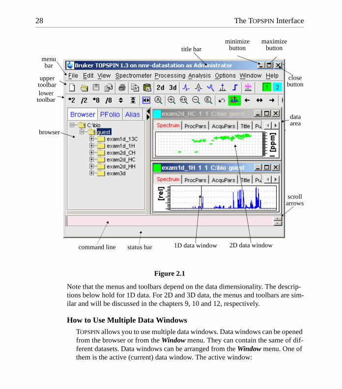
The TOPSPIN window consist of several areas, bars, fields and buttons. The main part is a split pane which consists of the data area and the browser. Note that the browser can be inactive [hit Ctrl+d] or displayed as a separate window.
Fig. 2.1 shows the Topspin window with two data windows in the data area and the browser as an integral part.
28 The TOPSPIN Interface
DONE
INDEX
INDEX
Note that the menus and toolbars depend on the data dimensionality. The descrip-tions below hold for 1D data. For 2D and 3D data, the menus and toolbars are sim-ilar and will be discussed in the chapters 9, 10 and 12, respectively.
How to Use Multiple Data Windows
TOPSPIN allows you to use multiple data windows. Data windows can be opened from the browser or from the Window menu. They can contain the same of dif-ferent datasets. Data windows can be arranged from the Window menu. One of them is the active (current) data window. The active window:
Figure 2.1
closebutton
browser
title bar
dataarea
status bar
uppertoolbar lower
toolbar
menubar
maximizebutton
minimizebutton
2D data window
scrollarrows
command line 1D data window

The TOPSPIN Interface 29
DONE
INDEX
INDEX
• can be selected by clicking inside the window or hitting F6 repeatedly.
• has a highlighted title bar
• has the mouse focus
• is affected by menu, toolbar and command line commands
A cursor line (1D) or crosshair (2D) is displayed in all data windows at the same position. Moving the mouse affects the cursor in all data windows.
How to Use the Title bar
In the title bar you can:
• Left-click-hold & drag to move the window
• Double-click to maximize the window
• Right-click to open the title bar menu.
• Access the minimize, maximize and close buttons at the right
• Access the title bar menu button at the left
How to Use the Menu barThe menu bar contains the following menus:
• File : performing data/file handling tasks
• Edit : copy & paste data and finding data
• View : display properties, browser on/off, notebook
• Spectrometer : data acquisition and acquisition related tasks
• Processing : data processing
• Analysis : data analysis
• Options : setting various options, preferences and configurations
• Window : data window handling/arrangement
• Help : access various manuals.
Experienced users will usually work with keyboard commands rather than menu commands. Note that the main keyboard commands are displayed in square brackets [] behind the corresponding menu entries. Furthermore, right-clicking any menu entry will show the corresponding command.
30 The TOPSPIN Interface
DONE
INDEX
INDEX
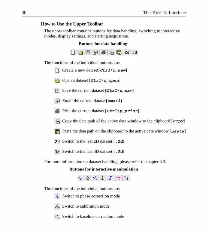
How to Use the Upper Toolbar
The upper toolbar contains buttons for data handling, switching to interactive modes, display settings, and starting acquisition.
Buttons for data handling:
The functions of the individual buttons are:
Create a new dataset[Ctrl+n, new]
Open a dataset [Ctrl+o, open]
Save the current dataset [Ctrl+s, sav]
Email the current dataset[smail]
Print the current dataset [Ctrl+p, print]
Copy the data path of the active data window to the clipboard [copy]
Paste the data path on the clipboard to the active data window [paste]
Switch to the last 2D dataset [.2d]
Switch to the last 3D dataset [.3d]
For more information on dataset handling, please refer to chapter 4.3.
Buttons for interactive manipulation
The functions of the individual buttons are:
Switch to phase correction mode
Switch to calibration mode
Switch to baseline correction mode

The TOPSPIN Interface 31
DONE
INDEX
INDEX
Switch to peak picking mode
Switch to integration mode
Switch to multiple display mode
Switch to distance measurement mode
For more information on interactive manipulation, refer to chapter 11 and 12.
Buttons for display options
The functions of the individual buttons are:
Toggle between Hz and ppm axis units
Switch the y-axis display between abs/rel/off
Switch the overview spectrum on/off
Toggle grid between fixed/axis/off
For more information on display options, please refer to chapter 8.5 and 9.5.
How to Use the Lower Toolbar
The lower toolbar contains buttons for display manipulations.
Buttons for vertical scaling (intensity manipulation)
Increase the intensity by a factor of 2 [*2]
Decrease the intensity by a factor of 2 [/2]
Increase the intensity by a factor of 8 [*8]
Decrease the intensity by a factor of 8 [/8]
32 The TOPSPIN Interface
DONE
INDEX
INDEX
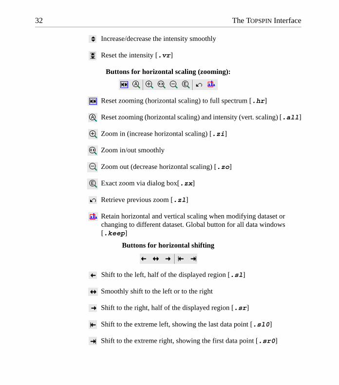
Increase/decrease the intensity smoothly
Reset the intensity [.vr]
Buttons for horizontal scaling (zooming):
Reset zooming (horizontal scaling) to full spectrum [.hr]
Reset zooming (horizontal scaling) and intensity (vert. scaling) [.all]
Zoom in (increase horizontal scaling) [.zi]
Zoom in/out smoothly
Zoom out (decrease horizontal scaling) [.zo]
Exact zoom via dialog box[.zx]
Retrieve previous zoom [.zl]
Retain horizontal and vertical scaling when modifying dataset or changing to different dataset. Global button for all data windows [.keep]
Buttons for horizontal shifting
Shift to the left, half of the displayed region [.sl]
Smoothly shift to the left or to the right
Shift to the right, half of the displayed region [.sr]
Shift to the extreme left, showing the last data point [.sl0]
Shift to the extreme right, showing the first data point [.sr0]

The TOPSPIN Interface 33
DONE
INDEX
INDEX
Buttons for vertical shifting
Shift the spectrum baseline to the middle of the data field [.su]
Smoothly shift the spectrum baseline up or down.
Shift the spectrum baseline to the bottom of the data field [.sd]
2.2 Command Line Usage
How to Put the Focus in the Command Line
In order to enter a command on the command line, the focus must be there. Note that, for example, selecting a dataset from the browser, puts the focus in the browser. To put the focus on the command line:
! Hit the Esc key
or
! Click inside the command line
How to Retrieve Previously Entered Commands
All commands that have been entered on the command line since TOPSPIN was started are stored and can be retrieved. To do that:
! Hit the ↑ (Up-Arrow) key on the keyboard
By hitting this key repeatedly, you can go back as far as you want in retrieving previously entered commands. After that you can go forward to more recently en-tered commands as follows:
! Hit the ↓ (Down-Arrow) key on the keyboard
How to Change Previously Entered Commands1. Hit the ← (Left-Arrow) or → (Right-Arrow) key to move the cursor
2. Add characters or hit the Backspace key to remove characters
3. Mark characters and use Backspace or Delete to delete them, Ctrl+c
34 The TOPSPIN Interface
DONE
INDEX
INDEX
to copy them, or Ctrl+v to paste them.
In combination with the arrow-up/down keys, you can edit previously entered commands.
How to Enter a Series of Commands
If you want to execute a series of commands on a dataset, you can enter the com-mands on the command line separated by semicolons, e.g.:
em;ft;apk
If you intend to use the series regularly, you can store it in a macro as follows:
! right-click in the command line and choose Save as macro.
2.3 Command Line History
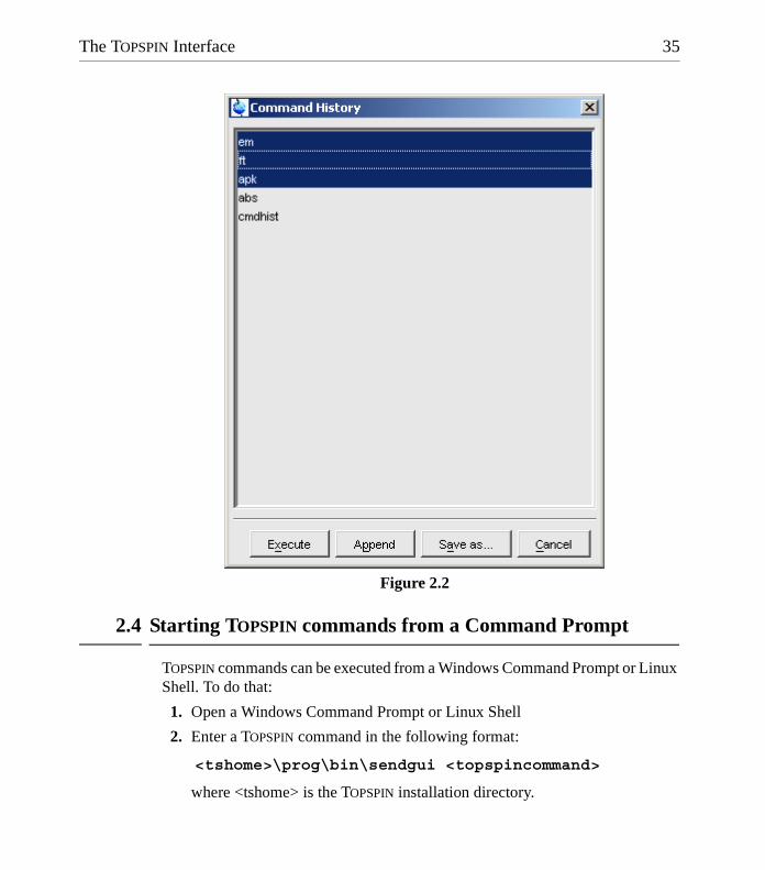
TOPSPIN allows you to easily view and reuse all commands, which were previ-ously entered on the command line. To open a command history control win-dow; click View " Command Line History, or right-click in the command line and choose Command Line History, or enter the command cmdhist (see Fig. 2.2).
It shows all commands that have been entered on the command line since TOP-SPIN was started. You can select one or more commands and apply one of the fol-lowing functions:
Execute
Execute the selected command(s).
Append
Append the (first) selected command to the command line. The appended command can be edited and executed. Useful for commands with many arguments such as re.
Save as..
The selected command(s) are stored as a macro. You will be prompted for the macro name. To edit this macro, enter edmac <macro-name>. To ex-ecute it, just enter its name on the command line.
The TOPSPIN Interface 35
DONE
INDEX
INDEX
2.4 Starting TOPSPIN commands from a Command Prompt
TOPSPIN commands can be executed from a Windows Command Prompt or Linux Shell. To do that:
1. Open a Windows Command Prompt or Linux Shell
2. Enter a TOPSPIN command in the following format:
<tshome>\prog\bin\sendgui <topspincommand>
where <tshome> is the TOPSPIN installation directory.
Figure 2.2
36 The TOPSPIN Interface
DONE
INDEX
INDEX
Examples:
C:\ts1.3\prog\bin\sendgui re exam1d_1H 1 1 C:/bio joe
reads the dataset C:/bio/joe/nmr/exam1d_13C/1/pdata/1.
C:\ts1.3\prog\bin\sendgui ft
executes a 1D Fourier transform.
Commands are executed on the currently active data window.
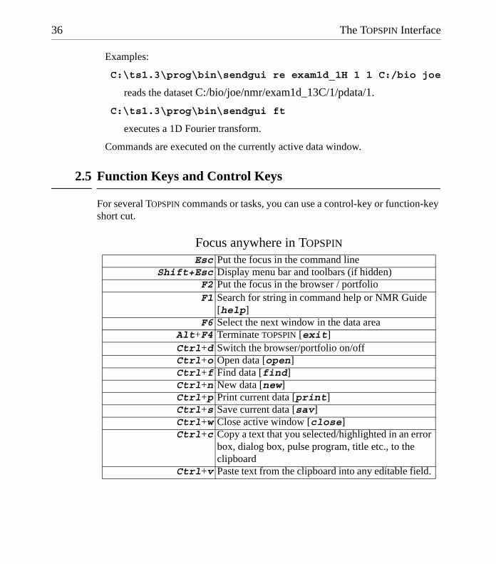
2.5 Function Keys and Control Keys
For several TOPSPIN commands or tasks, you can use a control-key or function-key short cut.
Focus anywhere in TOPSPIN
Esc Put the focus in the command lineShift+Esc Display menu bar and toolbars (if hidden)
F2 Put the focus in the browser / portfolioF1 Search for string in command help or NMR Guide
[help]F6 Select the next window in the data area
Alt+F4 Terminate TOPSPIN [exit]Ctrl+d Switch the browser/portfolio on/offCtrl+o Open data [open]Ctrl+f Find data [find]Ctrl+n New data [new]Ctrl+p Print current data [print]Ctrl+s Save current data [sav]Ctrl+w Close active window [close]Ctrl+c Copy a text that you selected/highlighted in an error
box, dialog box, pulse program, title etc., to the clipboard
Ctrl+v Paste text from the clipboard into any editable field.

The TOPSPIN Interface 37
DONE
INDEX
INDEX
Focus in the Command Line
Focus in the Browser/Portfolio
Focus anywhere in TOPSPIN
Ctrl+Backspace Kill current inputCtrl+Delete Kill current input
UpArrow Select previous command (if available).DownArrow Select next command (if available).
UpArrow Select previous datasetDownArrow Select next dataset
Enter In the Browser: expand selected nodeEnter In the Portfolio: display selected data
Scaling DataAlt+PageUp Scale up the data by a factor of 2 [*2]
Alt+PageDown Scale down the data by a factor 2 [/2]Ctrl+Alt+PageUp Scale up by a factor of 2, in all data windows
Ctrl+Alt+PageDown Scale down by a factor of 2, in all data windowsAlt+Enter Perform a vertical reset
Ctrl+Alt+Enter Perform a vertical reset in all data windowsZooming data
Alt+Plus Zoom in [.zi]Alt+Minus Zoom out [.zo]
Ctrl+Alt+Plus Zoom in, in all data windows Ctrl+Alt+Minus Zoom out, in all data windows
Shifting DataAlt+UpArrow Shift spectrum up [.su]
Alt+DownArrow Shift spectrum down [.sd]Alt+LeftArrow Shift spectrum to the left [.sl]Alt+RightArrow Shift spectrum to the right [.sr]
Ctrl+Alt+UpArrow Shift spectrum up, in all data windowsCtrl+Alt+DownArrow Shift spectrum down, in all data windowsCtrl+Alt+LeftArrow Shift spectrum to the left, in all data windows
Ctrl+Alt+RightArrow Shift spectrum to the right, in all data windows

38 The TOPSPIN Interface
DONE
INDEX
INDEX
Focus in a Table (e.g. peaks, integrals, nuclei, solvents)
Focus in a Plot Editor
Note that the function of function keys can be changed as described in chapter 2.7.
delete Delete the selected entrieshome Select the first entryend Select the last entry
Shift+Home Select the current and first entry and all in betweenShift+End Select the current and last entry and all in betweenDownArrow Select next entry
UpArrow Select previous entryCtrl+a Select all entriesCtrl+c Copy the selected entries to the clipboardCtrl+z Undo last action Ctrl+y Redo last undo action
F1 Open the Plot Editor Manual F5 Refresh
ctrl+F6 Display next layout ctrl+Shift+F6 Display previous layout
Ctrl+tab Display next layout delete Delete the selected objectsCtrl+a Select all objectsCtrl+i Open TOPSPIN InterfaceCtrl+c Copy the selected object from the ClipboardCtrl+l Lower the selected objectCtrl+s Save the current layoutCtrl+m Unselect all objectsCtrl+n Open a new layoutCtrl+o Open an existing layoutCtrl+p Print the current layoutCtrl+r Raise the selected objectCtrl+t Reset X and Y scaling of all marked objectsCtrl+v Paste the object from the Clipboard Ctrl+w Open the attributes dialog window.Ctrl+x Cut the selected object and place it on the Clipboard Ctrl+z Undo the last action
The TOPSPIN Interface 39
DONE
INDEX
INDEX
2.6 Help in Topspin
TOPSPIN offers help in various ways like online manuals, command help and toolt-ips.
How to Open Online Help documentsThe online help manuals can be opened from the Help menu. For example, to open the manual that you are reading now:
! Click Help " User’s Guide
To open the Avance Beginners Guide guide:
! Click Help " Avance Beginners Guide
To open the Processing Reference guide:
! Click Help " Processing Reference Manual
Note that most manuals are stored in the directory:
<tshome>/prog/docu/english/xwinproc/pdf
The most recent versions can be downloaded from:
www.bruker-biospin.de
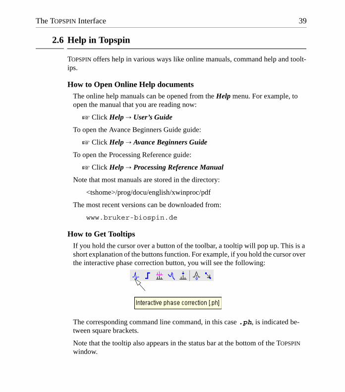
How to Get Tooltips
If you hold the cursor over a button of the toolbar, a tooltip will pop up. This is a short explanation of the buttons function. For example, if you hold the cursor over the interactive phase correction button, you will see the following:
The corresponding command line command, in this case .ph, is indicated be-tween square brackets.
Note that the tooltip also appears in the status bar at the bottom of the TOPSPIN window.

40 The TOPSPIN Interface
DONE
INDEX
INDEX
How to Get Help on Individual Commands
To get help on an individual command, for example ft:
! Enter ft?
or
! Enter help ft
In both cases, the HTML page with a description of the command will be opened.
Note that some commands open a dialog box with a Help button. Clicking this button will show the same description as using the help command. For example, entering re and clicking the Help button in the appearing dialog box
opens the same HTML file as entering help re or re?.
How to Use the Command Index
To open the TOPSPIN command index:
! Enter cmdindex
or
! Click Help " Command Index
From there you can click any command and jump to the corresponding help page.
The TOPSPIN Interface 41
DONE
INDEX
INDEX
2.7 User Defined Functions Keys
The default assignment of functions keys is described in chapter 2.5 and in the document:
! Help " Control and function keys
You may assign your own commands to functions keys. Here is an example of how to do that:
1. Open the file cmdtab_user.prop, located in the subdirectory userde-fined of the user properties directory (to locate this directory, enter hist and look for the entry "User properties directory=" ). The file cmdtab_user.prop is initially empty and can be filled with your own command definitions.
2. Insert e.g. the following lines into the file:
_f3=$em_f3ctrl=$ft_f3alt=$pk_f5=$halt_f5ctrl=$reb_f5alt=$popt
3. Restart TOPSPIN
Now, when you hit the F3 key, the command em will be executed. In the same way, Ctrl+F3, Alt+F3, F5, Ctrl+F5 and Alt+F5 will execute the com-mands ft, pk, halt, reb and popt, respectively. You can assign any com-mand, macro, AU program or Python program to any function keys. Only the keys Alt+F4, F6, Ctrl+F6, and Alt+F6 are currently fixed. Their function cannot be changed.
2.8 How to Open Multiple TOPSPIN Interfaces
TOPSPIN allows you to open multiple User Interfaces. This is, for example, useful to run an acquisition in one interface and process data in another. To open an addi-tion interface, enter the command newtop on the command line or click Window " New Topspin. To open yet another interface, enter newtop in the first or in the second interface. The display in each interface is completely independent from the others. As such, you can display different datasets or different aspects of the same

dataset, e.g. raw/processed, regions, scalings etc. When the dataset is (re)processed in one interface, its display is automatically updated in all TOPSPIN interfaces.
The command exit closes the current Topspin interface. Interfaces that were opened from this interface remain open. Entering exit in the last open TOPSPIN interface, finishes the entire TOPSPIN session. The position and geometry of each TOPSPIN interface is saved and restored after restart.
Chapter 4
Dataset Handling
4.1 The Topspin Browser and Portfolio
TOPSPIN offers a data browser/portfolio from which you can browse, select, and open data. Furthermore it allows you to define and list alias names for data. The browser appears at the left of the TOPSPIN window and can be controlled from the View menu.
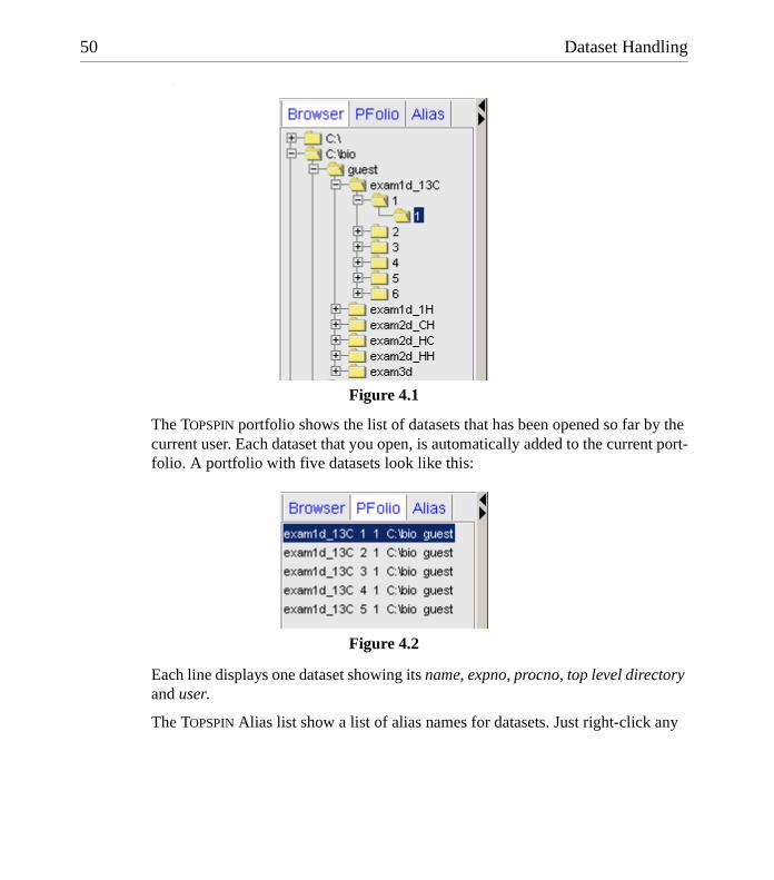
The browser is similar to the Windows Explorer. It shows data directory trees and allows you to expand/collapse their elements. Figure 4.1 shows a TOPSPIN browser with one top level data directory and one dataset fully expanded.
50 Dataset Handling
DONE
INDEX
INDEX
:
The TOPSPIN portfolio shows the list of datasets that has been opened so far by the current user. Each dataset that you open, is automatically added to the current port-folio. A portfolio with five datasets look like this:
Each line displays one dataset showing its name, expno, procno, top level directory and user.
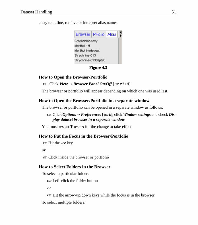
The TOPSPIN Alias list show a list of alias names for datasets. Just right-click any
Figure 4.1
Figure 4.2
Dataset Handling 51
DONE
INDEX
INDEX
entry to define, remove or interpret alias names.
How to Open the Browser/Portfolio
! Click View " Browser Panel On/Off [Ctrl+d]
The browser or portfolio will appear depending on which one was used last.
How to Open the Browser/Portfolio in a separate windowThe browser or portfolio can be opened in a separate window as follows:
! Click Options " Preferences [set], click Window settings and check Dis-play dataset browser in a separate window.
You must restart TOPSPIN for the change to take effect.
How to Put the Focus in the Browser/Portfolio
! Hit the F2 key
or
! Click inside the browser or portfolio
How to Select Folders in the Browser
To select a particular folder:
! Left-click the folder button
or
! Hit the arrow-up/down keys while the focus is in the browser
To select multiple folders:
Figure 4.3

52 Dataset Handling
DONE
INDEX
INDEX
! Hold the Ctrl key and left-click multiple folders to select them
or
! Hold the Shift key and left-click two folders to select these two and all in between.
How to Expand/Collapse a Folder in the BrowserTo expand a collapsed folder:
! Click the + button to the left of the folder button
or Double-click the folder button
or Hit the Right-Arrow key while the folder is highlighted
or Right-click the folder button and choose Expand fully from the popup menu to fully expand the folder
To collapse an expanded folder:
! Click the - button to the left of the folder button
or Double-click the folder button
or Hit the Left-Arrow key while the folder is highlighted
How to Expand a Folder showing Pulse program and Title! Right-click the data name folder button and choose
Expand fully & show PULPROG /Title from the popup menu
Fig. 4.4 shows an example of an expanded dataset showing the pulse program and title.
Figure 4.4
Dataset Handling 53
DONE
INDEX
INDEX
Note that collapsing the data name folder will deselect the display of the pulse program and title.
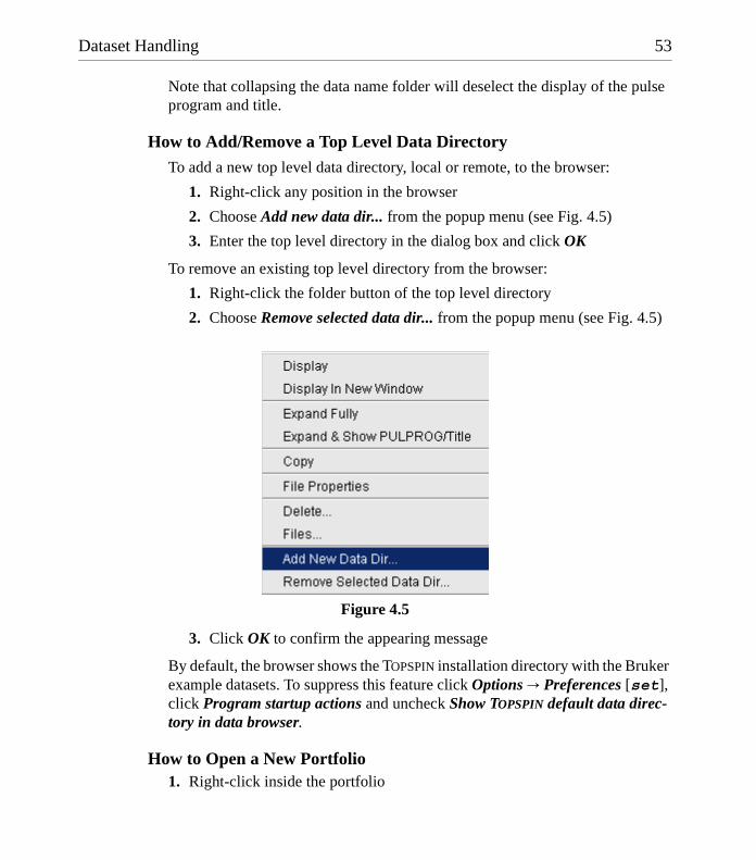
How to Add/Remove a Top Level Data DirectoryTo add a new top level data directory, local or remote, to the browser:
1. Right-click any position in the browser
2. Choose Add new data dir... from the popup menu (see Fig. 4.5)
3. Enter the top level directory in the dialog box and click OK
To remove an existing top level directory from the browser:
1. Right-click the folder button of the top level directory
2. Choose Remove selected data dir... from the popup menu (see Fig. 4.5)
3. Click OK to confirm the appearing message
By default, the browser shows the TOPSPIN installation directory with the Bruker example datasets. To suppress this feature click Options " Preferences [set], click Program startup actions and uncheck Show TOPSPIN default data direc-tory in data browser.
How to Open a New Portfolio1. Right-click inside the portfolio
Figure 4.5

54 Dataset Handling
DONE
INDEX
INDEX
2. Choose Open portfolio... from the appearing popup menu (see Fig. 4.6)
3. Navigate to the folder that contains the portfolio files
4. Select the desired portfolio file (extension .prop)
5. Click Open
How to Save the current Portfolio1. Right-click inside the portfolio.
2. Choose Save portfolio... from the appearing popup menu (see Fig. 4.6).
3. Specify a folder and filename in the appearing dialog box. The filename must have the extension .prop.
4. Click Save.
How to Remove Datasets from the PortfolioTo remove a single dataset from the portfolio:
1. Right-click the dataset.
2. Choose Remove from portfolio...from the popup menu (see Fig. 4.6).
3. Click OK in the appearing alert box.
To remove multiple datasets from the portfolio:
1. Hold the Ctrl key and left-click several datasets to select them or holdthe Shift key and left-click two datasets to select these two and all inbetween.
2. Right-click any of the selected datasets.
3. Choose Remove from portfolio...from the popup menu (see Fig. 4.6).
4. Click OK in the appearing alert box.
How to Find Data and Add them to the Portfolio1. Click Edit " Find data [Ctrl+f | find].
2. Specify the search criteria and click OK.
3. Select dataset(s) and click Add to portfolio.
How to Sort Data in the Portfolio1. Right-click inside the portfolio

Dataset Handling 55
DONE
INDEX
INDEX
2. Choose Sort mode from the popup menu (see Fig. 4.6).
3. Click Alphabetical to sort data in alphabetical order
or
Click Recent first to sort data by date of last open.
How to Add, Remove or Interpret Alias NamesTo add an alias name:
1. Click the Alias tab in the browser.
Figure 4.6
56 Dataset Handling
DONE
INDEX
INDEX
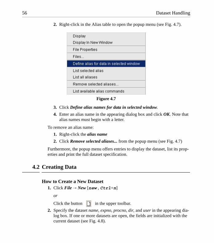
2. Right-click in the Alias table to open the popup menu (see Fig. 4.7).
3. Click Define alias names for data in selected window.
4. Enter an alias name in the appearing dialog box and click OK. Note that alias names must begin with a letter.
To remove an alias name:
1. Right-click the alias name
2. Click Remove selected aliases... from the popup menu (see Fig. 4.7)
Furthermore, the popup menu offers entries to display the dataset, list its prop-erties and print the full dataset specification.
4.2 Creating Data
How to Create a New Dataset1. Click File " New [new , Ctrl+n]
or
Click the button in the upper toolbar.
2. Specify the dataset name, expno, procno, dir, and user in the appearing dia-log box. If one or more datasets are open, the fields are initialized with the current dataset (see Fig. 4.8).
Figure 4.7
Dataset Handling 57
DONE
INDEX
INDEX
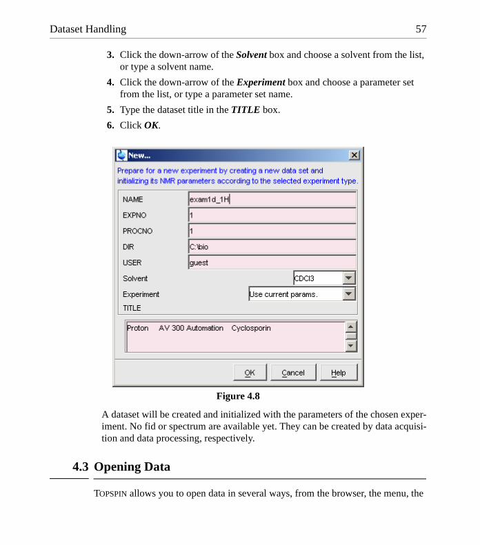
3. Click the down-arrow of the Solvent box and choose a solvent from the list, or type a solvent name.
4. Click the down-arrow of the Experiment box and choose a parameter set from the list, or type a parameter set name.
5. Type the dataset title in the TITLE box.
6. Click OK.
A dataset will be created and initialized with the parameters of the chosen exper-iment. No fid or spectrum are available yet. They can be created by data acquisi-tion and data processing, respectively.
4.3 Opening Data
TOPSPIN allows you to open data in several ways, from the browser, the menu, the
Figure 4.8

58 Dataset Handling
DONE
INDEX
INDEX
Explorer or the command line. Furthermore, data can be opened:
• in an existing data window replacing the current dataset.
• in a data window which is in multiple display mode, being superimposed on the current spectra.
• in a new data window which becomes the active window.
Note that if a dataset is already displayed in one window and it is opened in a sec-ond existing window, it still replaces the dataset in the latter one. As a result, the same dataset will be displayed in two windows (see also command reopen).
How to Open Data Windows CascadedBy default, a new data window appears maximized, filling the entire data field and covering possibly existing window. You can, however, configure TOPSPIN to open new windows cascaded. This is convenient if you want to open several data win-dows and then select one.
To open new windows cascaded:
1. Click Options " Preferences [set]
2. Click Window Setting in the left part of the dialog box.The right part of the dialog box shows the window settings (see Fig. 4.9).
3. Check Open new internal windows ’cascaded’ rather than ’max’.
4. Optionally you can configure the cascaded windows by clicking the respec-tive Change button. This will open the dialog box shown in Fig. 4.10.
Figure 4.9

Dataset Handling 59
DONE
INDEX
INDEX
5. Here you can specify the data window sizes and offsets as fractions of the maximum window sizes.
6. Click OK to close the dialog box.
How to Open Data from the BrowserIn the browser:
! Left-click-hold a data name, expno or procno and drag it into the data area. The data will be displayed in a new data window.
or Left-click-hold a data name, expno or procno and drag it into an open data window. The data will replace the currently displayed data.
or Left-click-hold a data name, expno or procno and drag it into an empty data window created with Alt+w n.
or Left-click-hold a data name, expno or procno and drag it into a multiple dis-play data window. The data will be superimposed on the currently dis-played data.
or Right-click a data name, expno or procno and choose Display from the pop-up menu; the data will be displayed in the current data window.
or Right-click a data name, expno or procno and choose Display in new win-
Figure 4.10
60 Dataset Handling
DONE
INDEX
INDEX
dow from the popup menu; the dataset will be displayed in a new data win-dow.
or Hold the Ctrl key and left-click several datasets to select them or hold the Shift key and left-click two datasets to select these two and all in be-tween. Then right-click one of the selected datasets and choose Display from the popup menu. A new window will be opened showing the selected datasets in multiple display mode. However, if the current window was al-ready in multiple display mode, the selected spectra will be superimposed on the currently displayed spectra.
How to Open Data from the Portfolio
The portfolio offers the same possibilities to open a dataset as the browser. Addi-tional options are:
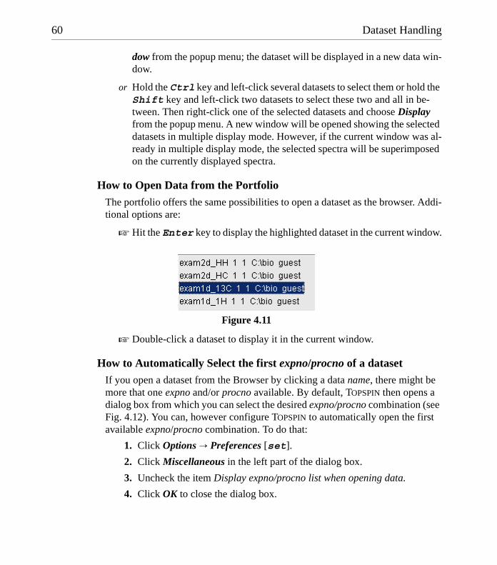
! Hit the Enter key to display the highlighted dataset in the current window.
! Double-click a dataset to display it in the current window.
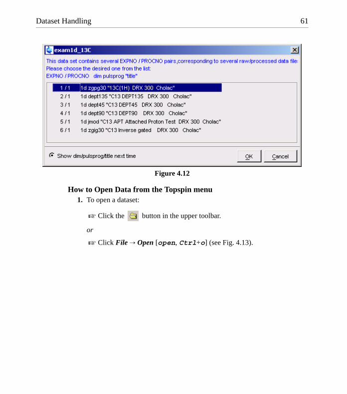
How to Automatically Select the first expno/procno of a datasetIf you open a dataset from the Browser by clicking a data name, there might be more that one expno and/or procno available. By default, TOPSPIN then opens a dialog box from which you can select the desired expno/procno combination (see Fig. 4.12). You can, however configure TOPSPIN to automatically open the first available expno/procno combination. To do that:
1. Click Options " Preferences [set].
2. Click Miscellaneous in the left part of the dialog box.
3. Uncheck the item Display expno/procno list when opening data.
4. Click OK to close the dialog box.
Figure 4.11
Dataset Handling 61
DONE
INDEX
INDEX
How to Open Data from the Topspin menu1. To open a dataset:
! Click the button in the upper toolbar.
or
! Click File " Open [open, Ctrl+o] (see Fig. 4.13).
Figure 4.12

62 Dataset Handling
DONE
INDEX
INDEX
2. In the appearing dialog box (see Fig. 4.14):
a) Select the option Open NMR data stored in standard Bruker format.
b) Select the browser type RE Dialog.
c) Click OK.
Figure 4.13
Figure 4.14
Dataset Handling 63
DONE
INDEX
INDEX
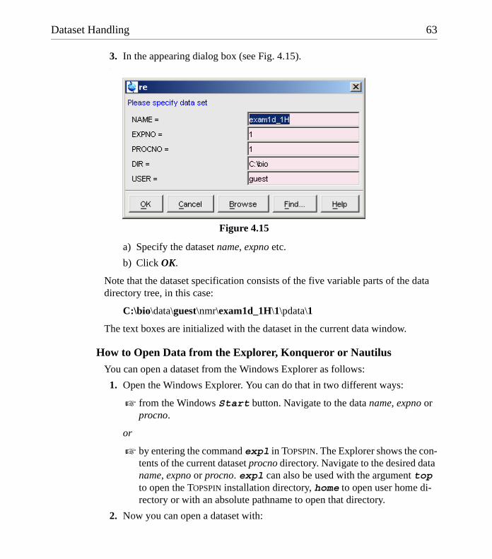
3. In the appearing dialog box (see Fig. 4.15).:
a) Specify the dataset name, expno etc.
b) Click OK.
Note that the dataset specification consists of the five variable parts of the data directory tree, in this case:
C:\bio\data\guest\nmr\exam1d_1H\1\pdata\1
The text boxes are initialized with the dataset in the current data window.
How to Open Data from the Explorer, Konqueror or Nautilus
You can open a dataset from the Windows Explorer as follows:
1. Open the Windows Explorer. You can do that in two different ways:
! from the Windows Start button. Navigate to the data name, expno or procno.
or
! by entering the command expl in TOPSPIN. The Explorer shows the con-tents of the current dataset procno directory. Navigate to the desired data name, expno or procno. expl can also be used with the argument top to open the TOPSPIN installation directory, home to open user home di-rectory or with an absolute pathname to open that directory.
2. Now you can open a dataset with:
Figure 4.15
64 Dataset Handling
DONE
INDEX
INDEX
! drag & drop: click-hold a dataset name or any of its sub-folders or files and drag it into the TOPSPIN data area or data window.
or
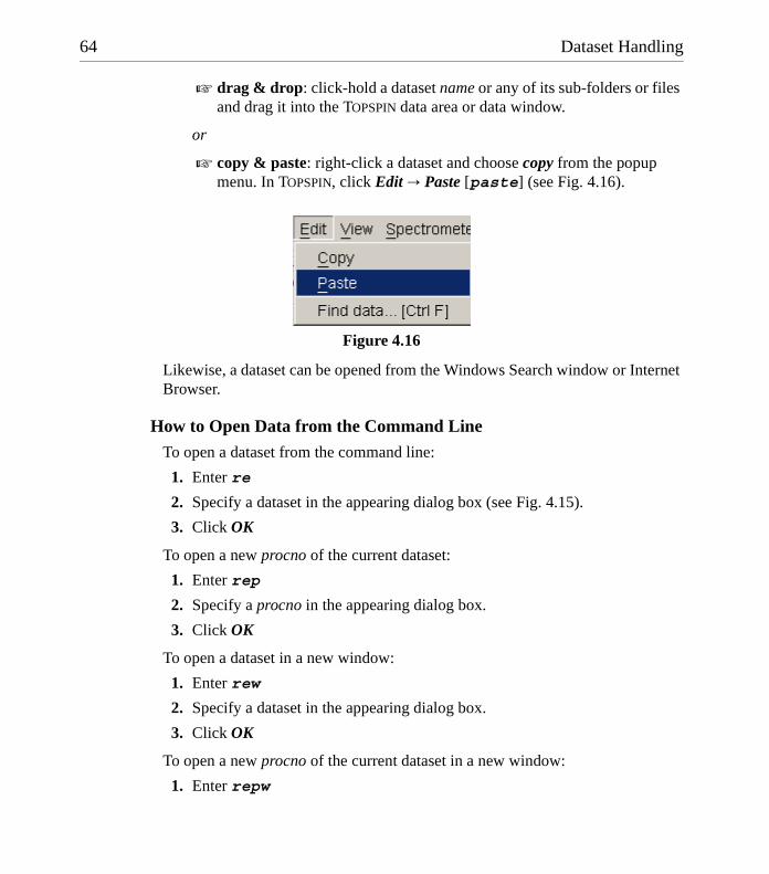
! copy & paste: right-click a dataset and choose copy from the popup menu. In TOPSPIN, click Edit " Paste [paste] (see Fig. 4.16).
Likewise, a dataset can be opened from the Windows Search window or Internet Browser.
How to Open Data from the Command LineTo open a dataset from the command line:
1. Enter re
2. Specify a dataset in the appearing dialog box (see Fig. 4.15).
3. Click OK
To open a new procno of the current dataset:
1. Enter rep
2. Specify a procno in the appearing dialog box.
3. Click OK
To open a dataset in a new window:
1. Enter rew
2. Specify a dataset in the appearing dialog box.
3. Click OK
To open a new procno of the current dataset in a new window:
1. Enter repw
Figure 4.16
Dataset Handling 65
DONE
INDEX
INDEX
2. Specify a procno in the appearing dialog box.
3. Click OK
To open a data browser and read a dataset from there:
1. Enter reb
2. Select a dataset from the appearing dialog box.
3. Click Display
Note that re, rep and reb:
• Replace the data in the currently selected data window.
• Open the data in a new window when they are used after typing Alt+w n
• Add the data in the currently selected window if this is in multiple display mode.
whereas rew and repw :
• Always open the dataset in a new window.
How to Open Special Format Data
Apart from the standard Bruker data format, TOPSPIN is able to read and display various other formats. To do this:
! Click File " Open [open, Ctrl+o]
select the option Open NMR data stored in special formats, select the desired file type (see Fig. 4.17) and click OK..
A dialog will appear which depends on the chosen file type. Just follow the in-structions on the screen.
The following file types are supported:
• JCAMP-DX - Bruker TOPSPIN1 data stored in JCAMP-DX format
• Zipped TOPSPIN - Bruker TOPSPIN data stored in ZIP format
• WINNMR - Bruker WINNMR data
• A3000 - Bruker Aspect 3000 data
1. Note that the TOPSPIN data format is identical to the XWIN-NMR data format.

66 Dataset Handling
DONE
INDEX
INDEX
• VNMR - data acquired on a Varian spectrometer
• JNMR - data acquired on a Jeol spectrometer
• Felix - 1D data, FID or spectrum, which are stored in FELIX format.
Note that in all cases, the data are stored in a single data file which is un-packed/converted to standard Bruker format, i.e. to a data directory tree.
How to Open a ZIP or JCAMP-DX file from the Windows Explorer
Data stored in ZIP or JCAMP-DX format can also be opened directly from the Windows Explorer. You can do that as follows:
! drag & drop: click-hold a file with the extension .dx or .zip and drag it into the TOPSPIN data area or data window.
! copy & paste: right-click a file with the extension .dx or .zip and choose copy from the popup menu. In TOPSPIN, click Edit " Paste[paste].
4.4 Saving/Copying Data
How to Save or Copy Data
You can save the current dataset as follows:
Figure 4.17

Dataset Handling 67
DONE
INDEX
INDEX
1. Click File " Save [Ctrl+s].
This will open a dialog box (see Fig. 4.18).
2. Select an option and, if applicable, a file type.
3. Click OK to execute the option.
The six options correspond to the following command line commands:
• wrpa - copies the current data to a new data name or expno
• tozip - convert a dataset of any dimension to ZIP format
• tojdx - convert a 1D or 2D dataset to JCAMP-DX format
• totxt - convert a 1D or 2D dataset text format
• wpar - write parameter set
• convdta - save digitally filtered data as analog filtered data
• wrp, wra, genfid, wmisc - write various files
How to Save an Entire Dataset1. Click File " Save [Ctrl+s].
Figure 4.18
68 Dataset Handling
DONE
INDEX
INDEX
2. Select the option Copy dataset to a new destination [wrpa] and click OK
3. Specify the dataset variables and click OK
How to Save Processed Data1. Click File " Save [Ctrl+s].
2. Select the option Save other file
3. Select File type Processed data as new procno [wrp] and click OK
4. Enter a processing number (procno) and click OK
How to Save Acquisition Data1. Click File " Save [Ctrl+s].
2. Select the option Save other file
3. Select File type Acqu. data as new expno [wra] and click OK
4. Enter a experiment number (expno) and click OK
How to Save Processed Data as Pseudo Raw Data1. Click File " Save [Ctrl+s]
2. Select the option Save other file
3. Select File type 1r/1i as fid [genfid] or 2rr/2ii as ser [genser]
4. Click OK
5. Enter a destination expno.
(optionally, you can specify further data path specifications)
6. Click OK
4.5 Deleting Data
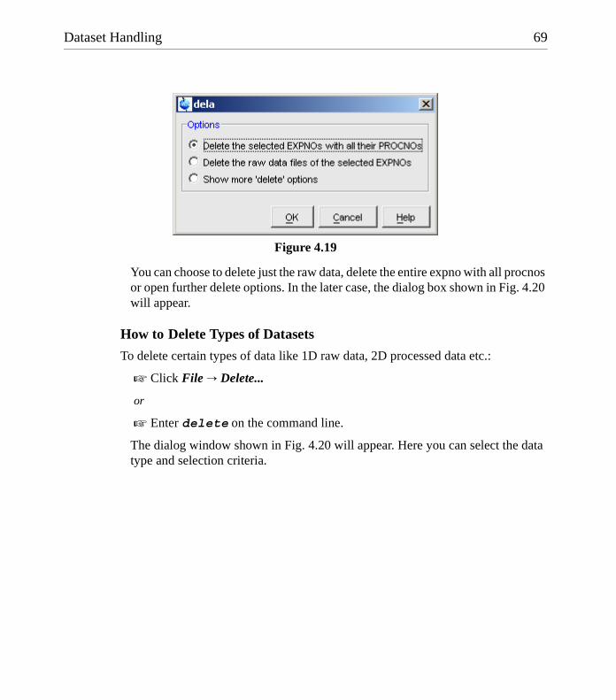
How to Delete a Specific Dataset
! Right-click the data name, expno or procno in the browser, then click Delete...
In each case, a delete dialog will appear. The dialog box for a data expno, for an is shown in Fig. 4.19.
Dataset Handling 69
DONE
INDEX
INDEX
You can choose to delete just the raw data, delete the entire expno with all procnos or open further delete options. In the later case, the dialog box shown in Fig. 4.20 will appear.
How to Delete Types of Datasets
To delete certain types of data like 1D raw data, 2D processed data etc.:
! Click File " Delete...
or
! Enter delete on the command line.
The dialog window shown in Fig. 4.20 will appear. Here you can select the data type and selection criteria.
Figure 4.19

70 Dataset Handling
DONE
INDEX
INDEX
:
1. Select a data type option
For each option, the corresponding command appears in the title of the dialog box. These commands can also be used to delete data from the command line.
2. Specify the Required parameters
Note that you can use the wildcards:
• Asterix (*) for any character and any number of characters.
• Question mark (?) for any single character.
3. Click OK
A dialog box will appear showing the matching datasets. For example, if you se-lect the option An entire dataset ... :
1. Select dataset entries for deletion (selected entries are highlighted).
Figure 4.20
Dataset Handling 71
DONE
INDEX
INDEX
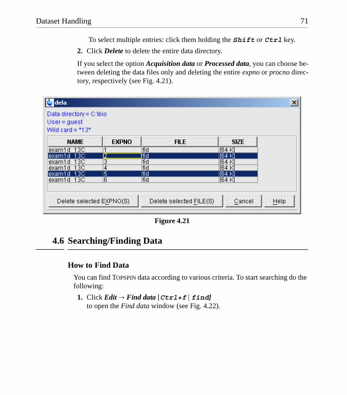
To select multiple entries: click them holding the Shift or Ctrl key.
2. Click Delete to delete the entire data directory.
If you select the option Acquisition data or Processed data, you can choose be-tween deleting the data files only and deleting the entire expno or procno direc-tory, respectively (see Fig. 4.21).
4.6 Searching/Finding Data
How to Find Data
You can find TOPSPIN data according to various criteria. To start searching do the following:
1. Click Edit " Find data [Ctrl+f | find]to open the Find data window (see Fig. 4.22).
Figure 4.21

72 Dataset Handling
DONE
INDEX
INDEX
2. Specify the search criteria. Note that:
• Dataset variables are searched that contain the specified string.
• Search is restricted to data created between the specified dates. Note that the acquisition date is evaluated.
The Reset mask button resets the default criteria.
3. Click OKto get a list of data that fulfil these criteria (see Fig. 4.23).
Figure 4.22
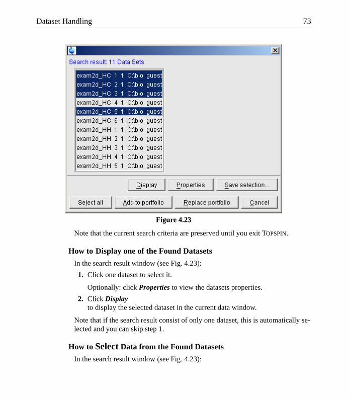
Dataset Handling 73
DONE
INDEX
INDEX
Note that the current search criteria are preserved until you exit TOPSPIN.
How to Display one of the Found Datasets
In the search result window (see Fig. 4.23):
1. Click one dataset to select it.
Optionally: click Properties to view the datasets properties.
2. Click Displayto display the selected dataset in the current data window.
Note that if the search result consist of only one dataset, this is automatically se-lected and you can skip step 1.
How to Select Data from the Found Datasets
In the search result window (see Fig. 4.23):
Figure 4.23

74 Dataset Handling
DONE
INDEX
INDEX
! Hold the Ctrl key and left-click several datasets to select these datasets.
or
! Hold the Shift key and left-click two datasets to select these datasets and all datasets in between.
or
! Click Select all to select all datasets in the search result.
How to Add Selected Datasets to the Portfolio1. Select the desired dataset(s) as described above.
2. To add them to the portfolio:
! Click Add to portfolio to extend the current portfolio.
or
! Click Replace portfolio to replace the current portfolio.
How to Save Selected Datasets to a List1. Select the desired dataset(s) as described above.
2. Click Save selection...
3. In the appearing browser:
a) Navigate to the desired list directory.
b) Enter or select the list filename.
c) Click OK
Dataset lists can be used by the acquisition or by serial processing (command serial).
4.7 Handling Data Files
How to List/Open the Current Dataset Files
A Bruker dataset is represented by a directory tree which contains files in the ex-pno and procno subdirectories. These files contain the actual data, parameters, lists etc.
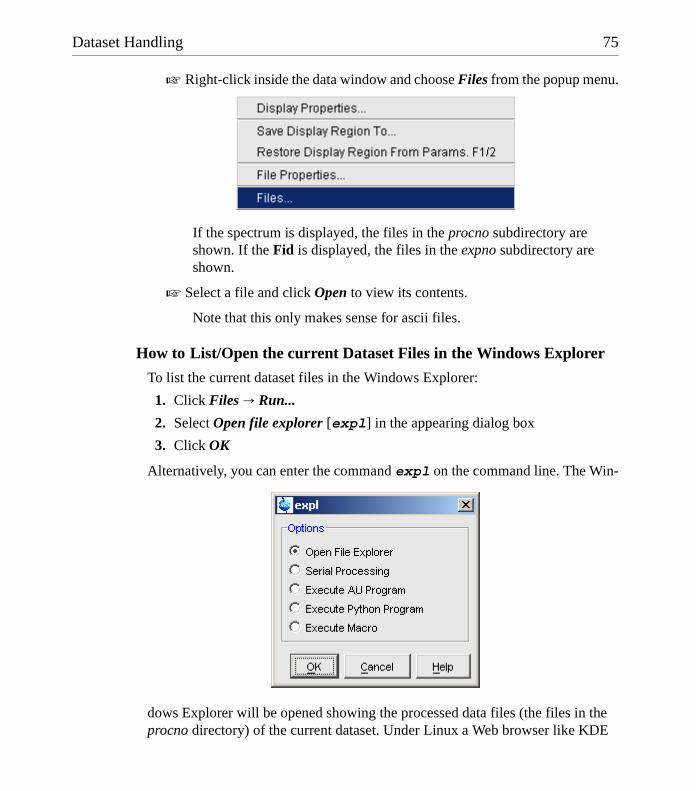
Dataset Handling 75
DONE
INDEX
INDEX
! Right-click inside the data window and choose Files from the popup menu.
If the spectrum is displayed, the files in the procno subdirectory are shown. If the Fid is displayed, the files in the expno subdirectory are shown.
! Select a file and click Open to view its contents.
Note that this only makes sense for ascii files.
How to List/Open the current Dataset Files in the Windows Explorer
To list the current dataset files in the Windows Explorer:
1. Click Files " Run...
2. Select Open file explorer [expl] in the appearing dialog box
3. Click OK
Alternatively, you can enter the command expl on the command line. The Win-
dows Explorer will be opened showing the processed data files (the files in the procno directory) of the current dataset. Under Linux a Web browser like KDE

76 Dataset Handling
DONE
INDEX
INDEX
Konqueror or Gnome Mozilla will be opened.
To open a file:
! Double-click the file or right-click the folder icon and choose Open
If TOPSPIN data area contains no datasets, the expl command opens the Explorer showing the users home directory. When entered on the command line, expl can also be used with the argument top to open the TOPSPIN installation directory, home to open user home directory or with an absolute pathname to open that di-rectory.
4.8 Data Consistency Check
TOPSPIN maintains audit trail files for compliance with GLP, GMP and FDA requirements.
The processing command that creates processed data from the raw data, e.g. em, creates the processing audit trail file auditp.txt and inserts the first entry. Any processing command that modifies/updates the processed data, e.g. ft, makes an additional entry. Furthermore, any command that changes one or more processing status parameters makes an additional entry. The audit trail can be checked with the command audit. This command opens a dialog box (see Fig. 4.24).
The first two entries allow you to view the audit trail files. The third entry per-forms an audit trail check, i.e. a data consistency check. If both raw and processed
Figure 4.24
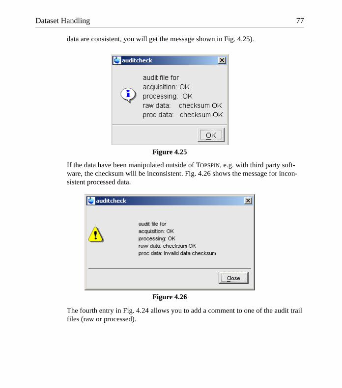
Dataset Handling 77
DONE
INDEX
INDEX
data are consistent, you will get the message shown in Fig. 4.25).
If the data have been manipulated outside of TOPSPIN, e.g. with third party soft-ware, the checksum will be inconsistent. Fig. 4.26 shows the message for incon-sistent processed data.
The fourth entry in Fig. 4.24 allows you to add a comment to one of the audit trail files (raw or processed).
Figure 4.25
Figure 4.26


Chapter 5
Parameter Handling
5.1 Processing Parameters
Processing parameters can be set/changed in three different ways:
• from the parameter editor: click the ProcPars tab or enter edp
• from the command line: e.g. enter si
• from a command dialog box: e.g. wm
How to Set a Processing Parameter from the Command Line
Enter the parameter name on the command line. For example to set the size:
1. Enter si
for 1D data, the following dialog box will appear:
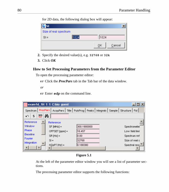
80 Parameter Handling
DONE
INDEX
INDEX
for 2D data, the following dialog box will appear:
2. Specify the desired value(s), e.g. 32768 or 32k
3. Click OK
How to Set Processing Parameters from the Parameter Editor
To open the processing parameter editor:
! Click the ProcPars tab in the Tab bar of the data window.
or
! Enter edp on the command line.
At the left of the parameter editor window you will see a list of parameter sec-tions.
The processing parameter editor supports the following functions:
Figure 5.1

Parameter Handling 81
DONE
INDEX
INDEX
! Enter (part of) a parameter name in the search field and click .
! Click a parameter section, e.g. Phase at the left of the dialog box. The sec-tion becomes highlighted and the corresponding parameters will appear in the right part of the dialog box.
! Click in a parameter field, e.g. PHC0, to set the parameter value.
! Hit the Tab key to jump to the next parameter field.
! Hit Shift+Tab to jump to the previous parameter field.
! Use the scroll bar at the right of the dialog box to move to parameters fur-ther up or down in the dialog box.
How to Undo the Last Processing Parameter Change
! Click the following button:
Undo last parameter change.
How to Display Processing Status Parameters
! Click the following button:
Show processing status parameters.
Note that the command dpp opens the parameter editor and automatically shows the status parameters.
How to Change Processed Data Dimensionality
! Click the following button:
Change data dimensionality.
This changes the number of parameter columns and value of the processing pa-rameter PPARMOD.
The parameter editor does not allow you to modify status parameters. Processing status parameters reflect the status of the processed data and are used for further processing, display or plotting. Changing them can make the dataset inconsistent. In rare cases, however, it can be useful to change a status parameter and TOPSPIN allows you to do that from the command line. If, for instance, you want to change the F1 status parameter MC2 of a 2D dataset, you have to enter:

82 Parameter Handling
DONE
INDEX
INDEX
s mc2
Note that the command s is used for 1D, 2D and 3D dataset. TOPSPIN automati-cally recognizes the dimensionality of the data and displays the parameter in all relevant dimensions. Note that, for example, the parameter MC2 only exists in F1.
5.2 Acquisition Parameters
How to Set Acquisition ParametersAcquisition parameters can be set/changed as follows:
• from the parameter editor: click the AcquPars tab or enter eda
• from the command line: e.g. enter td
• from the interactive parameter adjustment window (enter gs)
How to Set an Acquisition Parameter from the Command Line
Enter the parameter name on the command line. For example to set the time do-main size:
1. Enter td
for 1D data, the following dialog box will appear:
for 2D data, the following dialog box will appear:

Parameter Handling 83
DONE
INDEX
INDEX
2. Specify the desired value(s), e.g. 65536 or 64k
3. Click OK
How to Set Acquisition Parameters from the Parameter Editor
To open the acquisition parameter editor:
! Click the AcquPars tab in the Tab bar of the data window.
or
! Enter eda on the command line.
Fig. 5.2 shows an example of the acquisition parameter editor with the Experi-ment parameters displayed.
The processing parameter editor supports the following functions:
! Enter (part of) a parameter name in the search field and click .
! Click a parameter section, e.g. Experiment at the left of the dialog box. The section becomes highlighted and the corresponding parameters will appear in the right part of the dialog box.
! Click in a parameter field, e.g. TD, to set the parameter value.
! Hit the Tab key to jump to the next parameter field.
! Hit Shift+Tab to jump to the previous parameter field.
Figure 5.2

84 Parameter Handling
DONE
INDEX
INDEX
! Use the scroll bar at the right of the dialog box to move to parameters fur-ther up or down in the dialog box.
How to Undo the Last Acquisition Parameter Change
! Click the following button:
Undo last acquisition parameter change.
How to Set Pulse Program Parameters
! Click the following button:
Show pulse program parameters [ased]
The button will change to . To make this the default setting:
Click Options " Preferences, click Miscellaneous, check the entry "Show reduced parameter set (ased)" and click OK.
How to Display Acquisition Status Parameters
! Click the following button:
Show acquisition status parameters.
Note that the command dpa opens the acquisition parameter editor and automat-ically shows the status parameters.
How to Get Probehead/Solvent dependent Parameters! Click the following button:
Set probehead/solvent dependant parameters [getprosol].
Probehead and solvent dependant parameters can be set up with the command edprosol.
How to Change Acquisition Data Dimensionality
! Click the following button:
Change data dimensionality.
This changes the number of parameter columns and value of the acquisition pa-rameter PARMODE.
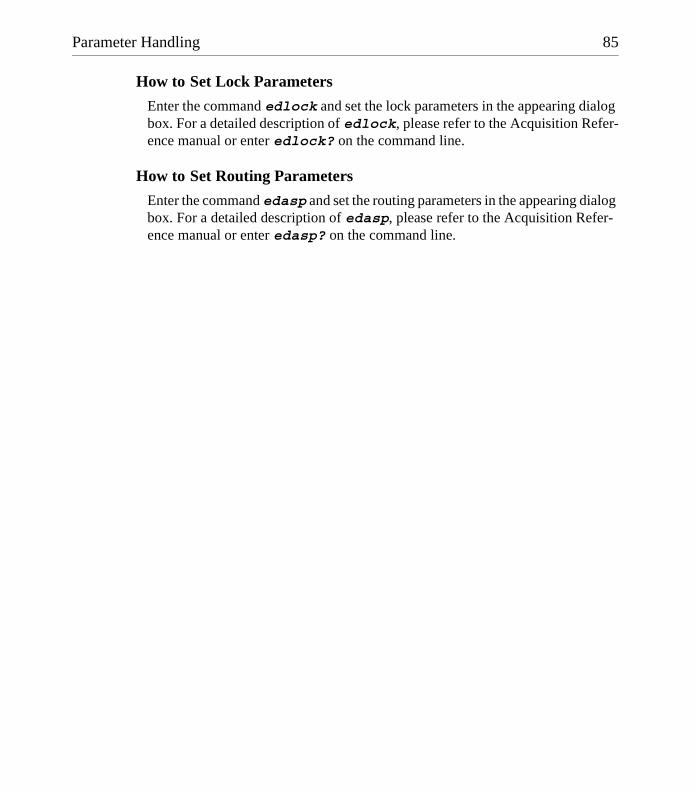
Parameter Handling 85
DONE
INDEX
INDEX
How to Set Lock Parameters
Enter the command edlock and set the lock parameters in the appearing dialog box. For a detailed description of edlock, please refer to the Acquisition Refer-ence manual or enter edlock? on the command line.
How to Set Routing Parameters
Enter the command edasp and set the routing parameters in the appearing dialog box. For a detailed description of edasp, please refer to the Acquisition Refer-ence manual or enter edasp? on the command line.


Chapter 6
Data Processing
6.1 Interactive Processing
Interactive processing allows full control over the processing sequence. However, it requires detailed knowledge about the required parameters (see chapter 5.1) and commands. Therefore, it is only suitable for the advanced user. New or intermedi-ate users are recommended to use the Processing Guide for semi-automatic processing (see chapter 6.2).
How to Process Data with Single Commands
Data can be processed by entering single commands on the command line. A typ-ical 1D processing sequence would be:
em : exponential window multiplication
ft : Fourier transform
apk : automatic phase correction
sref : automatic calibration (referencing)
abs : automatic baseline correction
This allows you full control over each individual processing step.
88 Data Processing
DONE
INDEX
INDEX
How to Process data with Composite Commands
Data can also be processed with so called composite commands. These are com-binations of single processing commands. The following composite commands are available.
• ef : Exponential multiplication + Fourier transform
• efp : Exponential multiplication + Fourier transform + phase correction
• fmc : Fourier transform + magnitude calculation
• fp : Fourier transform +phase correction
• gf : Gaussian multiplication + Fourier transform
• gfp : Gaussian multiplication + Fourier transform + phase correction
They can be entered on the command line or clicked from the menu. For the latter option:
! Click Processing " More transforms " Shortcuts
Just like single commands, composite commands can be used in Macros, AU pro-grams and Python programs.
6.2 Semi-automatic Processing
How to Use the Processing Guide in Automatic modeThe Processing Guide in automatic mode guides you through the entire process-ing sequence of data selection, processing, printing and archiving with minimum user interaction.
1. Click Processing " Processing Guide
The Processing Guide window will appear as an integral part of the current data window (see Fig. 6.1).

Data Processing 89
DONE
INDEX
INDEX
2. In the Processing Guide window:
a) Check Automatic mode
b) Click Open data set and click OK to open a dataset manually, e.g. fromthe browser or click Browse to open the File Chooser.
Figure 6.1
90 Data Processing
DONE
INDEX
INDEX
c) Click Window function " Fourier Transform " etc.
Each processing step will be executed without user interaction.
How to Use the Processing Guide in Interactive modeThe Processing Guide in interactive mode guides you through the entire process-ing sequence of data selection, processing, printing and archiving requiring some user interaction.
1. Click Processing " Processing Guide
The Processing Guide window will appear as an integral part of the current data window.
2. In the Processing Guide window:
a) Uncheck Automatic mode
b) Click Open data set and click OK to open a dataset manually, e.g. fromthe browser or click Browse to open the File Chooser.
c) Click Window function " Fourier Transform " etc.
For each step a dialog box will appear where you can enter options, parameters etc. For details on these items, please refer to the corresponding commands in the Processing Reference Guide.
6.3 Processing Data with AU programs
Data processing can be performed by using AU programs. An AU program is actu-ally a C-program which contains TOPSPIN commands (macros) and/or C-language statements. Various standard AU programs are delivered with TOPSPIN. A typical 1D processing AU program is proc_1d. A simplified version of this AU program is:
EFAPKSREFABSAUTOPLOTQUIT
It executes the commands ef, apk, sref, abs and autoplot. To run this AU

Data Processing 91
DONE
INDEX
INDEX
program, just enter proc_1d on the command line 1. You can create your own AU programs with the command edau. Note that an AU program must end with QUIT or QUITMSG("your message"), and that all statements must be specified in capital letters. For more information on AU programs, please refer to the AU pro-gram reference manual:
Click Help " Programming " AU programming
As an alternative to AU programs, you can also write Python programs, which allow you to use TOPSPIN commands, User Interface functions and Graphic func-tions. For more information:
! Click Help " Programming " Python Programming
6.4 Serial Processing using Python programs
TOPSPIN allows you to process a series of datasets using serial scripts. The dataset list and command(s) to be used can be easily setup from the TOPSPIN interface as follows. Enter the command serial on the command line. This will open the
1. Before you can use any Bruker AU program, expinstall must have been executed once.
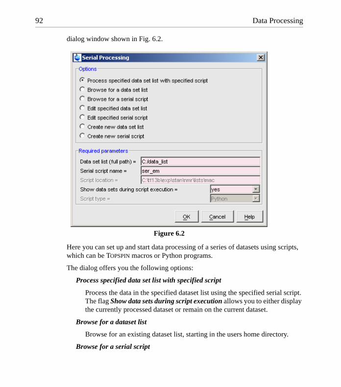
92 Data Processing
DONE
INDEX
INDEX
dialog window shown in Fig. 6.2.
Here you can set up and start data processing of a series of datasets using scripts, which can be TOPSPIN macros or Python programs.
The dialog offers you the following options:
Process specified data set list with specified script
Process the data in the specified dataset list using the specified serial script. The flag Show data sets during script execution allows you to either display the currently processed dataset or remain on the current dataset.
Browse for a dataset list
Browse for an existing dataset list, starting in the users home directory.
Browse for a serial script
Figure 6.2
Data Processing 93
DONE
INDEX
INDEX
Browse for existing serial script. Depending on the parameter Script type, the browser opens the ../exp/stan/nmr/py for Script type Python or ../exp/stan/nmr/lists/mac Script type macro. TOPSPIN, by default, searches for for files named ser_*.
Edit specified data set list
View or edit the list specified in the field Data Set List.
Edit specified serial script
View or edit the script specified in the field Serial script name
Create new data set list
Opens a dialog box for finding datasets. Proceed as follows:
1. Specify all search criteria and click OK
2. In the appearing Search result box:
a) Select the desired datasets.
b) Click Save selection..
3. In the appearing browser:
a) Navigate to the desired list directory.
b) Enter or select the list filename.
c) Click OK
Alternatively, you can create a dataset list manually.The format of a list entry is:
<name> <expno> <procno> <dir> <user>
An example of a dataset list is:
exam1d_13C 1 1 C:/bio guestexam1d_13C 2 1 C:/bio guestexam1d_13C 3 1 C:/bio guest
Create new serial script
Opens the appropriate editor to create a new script. For Script type Python, edpy is executed, for Script type macro, edmac is executed. The name of a se-rial script (macro of Python) must start with ser_. Python scripts must have the extension .py. A standard example is the python script ser_efp.py.
94 Data Processing
DONE
INDEX
INDEX
An example of a simple processing sequence is exponential window multiplica-tion, Fourier transform and automatic phase correction of a 1D dataset. A TOPSPIN macro performing this task would be:
ef
apk
A Python programs performing the same task would be:
EF()APK()
Note that Python programs are much more versatile than macros. Details on Python programming can be found under:
Help " Programming " Python programming
Note that serial processing can also be started as follows:
• Click Processing " Serial Processing...
or
• Click File " Run, select Execute Serial script on Data set list and click OK

Chapter 7
Printing/Exporting Data
7.1 Printing/plotting Data
How to Print/Plot from the Menu
The current data window can be printed as follows:
1. From the TOPSPIN menu:
! Click the button in the upper toolbar
or Click File " Print
or Enter print or Ctrl+p
All these actions are equivalent; they open the Print dialog box (see Fig. 7.1).
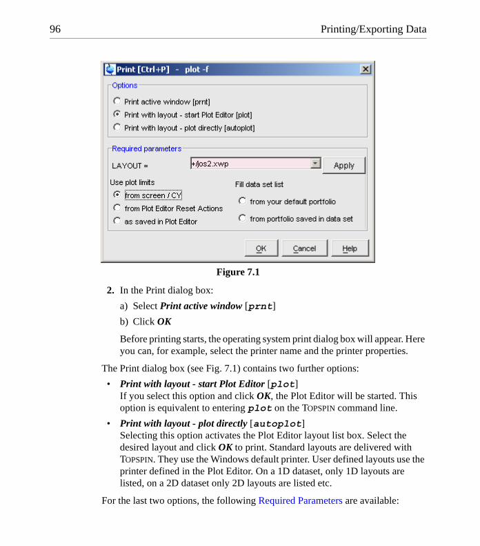
96 Printing/Exporting Data
DONE
INDEX
INDEX
2. In the Print dialog box:
a) Select Print active window [prnt]
b) Click OK
Before printing starts, the operating system print dialog box will appear. Here you can, for example, select the printer name and the printer properties.
The Print dialog box (see Fig. 7.1) contains two further options:
• Print with layout - start Plot Editor [plot]If you select this option and click OK, the Plot Editor will be started. This option is equivalent to entering plot on the TOPSPIN command line.
• Print with layout - plot directly [autoplot]Selecting this option activates the Plot Editor layout list box. Select the desired layout and click OK to print. Standard layouts are delivered with TOPSPIN. They use the Windows default printer. User defined layouts use the printer defined in the Plot Editor. On a 1D dataset, only 1D layouts are listed, on a 2D dataset only 2D layouts are listed etc.
For the last two options, the following Required Parameters are available:
Figure 7.1
Printing/Exporting Data 97
DONE
INDEX
INDEX
Use plot limits:
• from screen/ CYThe plot limits and maximum intensity are used as they are on the screen (processing parameter F1P, F2P and CY, respectively).
• from Plot Editor Reset ActionsThe plot limits and maximum intensity are set according to the Plot Editor Reset Actions (right-click inside the Plot Editor data field and choose Auto-mation to set the Reset Actions).
• as saved in Plot EditorThe plot limits and maximum intensity are set in the specified layout
Fill dataset list:
• from your default portfolioThe portfolio contains the current TOPSPIN dataset plus the data from the default Plot Editor portfolio.
• from port folio saved in datasetThe portfolio contains the current TOPSPIN dataset plus the data from the portfolio stored in this dataset.
How to Plot Data from the Processing guidePrinting/plotting data can be done from the Processing guide by clicking the Plot/Print button. If Automatic mode is checked, the active data window will be printed as it appears in the screen. If Automatic mode is unchecked, you will get the dialog box as displayed in Fig. 7.1.
How to Plot Data with the Plot EditorThe Plot Editor can be started from the Plot Editor or from the command line (command plot). The Plot Editor allows you to create layouts and plot data. The complete functionality is described in the online manual, which can be opened from the Plot Editor Help menu.
How to Print the Integral list1. Click the Integrals tab of the data window (see Fig. 7.2).
2. Enter print or Ctrl+p to print it.

98 Printing/Exporting Data
DONE
INDEX
INDEX
How to Print the Peak list1. Click the Peaks tab of the data window (see Fig. 7.3).
2. Enter print or Ctrl+p
Figure 7.2
Figure 7.3

Printing/Exporting Data 99
DONE
INDEX
INDEX
7.2 Exporting Data
How to Copy data to Other ApplicationsUnder MS Windows, you can easily copy the data window contents to other ap-plications. To do that:
! Click Edit " Copy [copy].
This will copy the data window contents to:
• the clipboard. After that you can paste the clipboard contents to any Win-dows application.
• the Windows Metafile file screenDump.wmf in the user properties directory (enter hist to locate this directory). The Windows Metafile can be imported by other applications or send to a different computer.
Please note:
Some programs, when importing spectra from the clipboard or metafile, do not display the contained information correctly. Particularly when you resize the im-ported graphics, sections of the text, the spectrum, or the axis sometimes have dis-appeared. Usually this is only a display problem. When you print the respective page, the representation is correct.
How to Store (Export) a Data Window as Graphics FileThe clipboard and metafile formats are resizable vector formats. In addition to this, TOPSPIN allows you to save the contents of a data window in a graphics file of selectable type, e.g. .png, .tif, .wmf etc. To do that:
1. Click File " Export.... [exportfile].
2. Navigate to the storage folder.
3. Enter the destination filename and extension.
4. Click Export
The resolution of such a screen dump equals the resolution of your screen.When you import a graphics file into an other program, you may loose information when resizing the graphics.

Chapter 8
1D Display
8.1 The 1D Data Window
The 1D data window consists of a data field, a title bar, a Tab bar and buttons. Fig. 8.1 shows a data window with a 1D spectrum.

102 1D Display
DONE
INDEX
INDEX
8.2 Displaying one Dataset in Multiple windows
TOPSPIN allows you to display one dataset in multiple data windows. This is, for example, convenient to view various regions or various objects (spectrum, fid, parameters etc.) of the same dataset.
How to Reopen a Dataset in a Second/Third etc. Window1. Select (activate) the desired dataset.
2. Click File " Reopen [reopen].
Multiple data windows with the same dataset are indicated with a number in square brackets, e.g. [1], in the title bar (see Fig. 8.2).
Figure 8.1
data field
closebutton title bar
Tab bar
maximizebutton
minimizebutton

1D Display 103
DONE
INDEX
INDEX
How to Rescale or Shift one Dataset in Multiple windows
Display manipulation buttons like and only work on the active data win-dow. The same counts for the keys Alt+PageUP and Alt+PageDown. How-ever, when used with the control key, they work on all windows, for example:
! Hit Ctrl+ , Ctrl+Alt+PageUp or Ctrl+Alt+PageDown
Figure 8.2

104 1D Display
DONE
INDEX
INDEX
8.3 Changing the Display of a 1D Spectrum or FID
TOPSPIN offers buttons to scale or shift the spectrum vertically and horizontally.
How to Change the Vertical Scaling of the FID or Spectrum
! Hit one of the following the keys:
• Alt+PageUp : Increase the intensity by a factor of 2.
• Alt+PageDown : Decrease the intensity by a factor of 2.
• Alt+Enter : Reset the intensity.
or
! Click-hold the button and move the mouse:
Change the intensity smoothly.
or
! Click one of the following buttons:
Increase the intensity by a factor of 2 [*2].
Increase the intensity by a factor of 8 [*8].
Decrease the intensity by a factor of 2 [/2].
Decrease the intensity by a factor of 8 [/8].
Reset the intensity [.vr].
Alternatively, you can enter the corresponding commands as specified between square brackets [].
To manipulate all data windows, press the Ctrl key while clicking one of the above buttons.
How to Change the Horizontal Scaling of the FID or Spectrum
! Click-hold the button and move the mouse:
Zoom in/out smoothly.
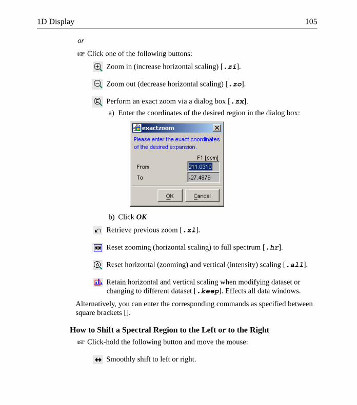
1D Display 105
DONE
INDEX
INDEX
or
! Click one of the following buttons:
Zoom in (increase horizontal scaling) [.zi].
Zoom out (decrease horizontal scaling) [.zo].
Perform an exact zoom via a dialog box [.zx].
a) Enter the coordinates of the desired region in the dialog box:
b) Click OK
Retrieve previous zoom [.zl].
Reset zooming (horizontal scaling) to full spectrum [.hr].
Reset horizontal (zooming) and vertical (intensity) scaling [.all].
Retain horizontal and vertical scaling when modifying dataset or changing to different dataset [.keep]. Effects all data windows.
Alternatively, you can enter the corresponding commands as specified between square brackets [].
How to Shift a Spectral Region to the Left or to the Right! Click-hold the following button and move the mouse:
Smoothly shift to left or right.
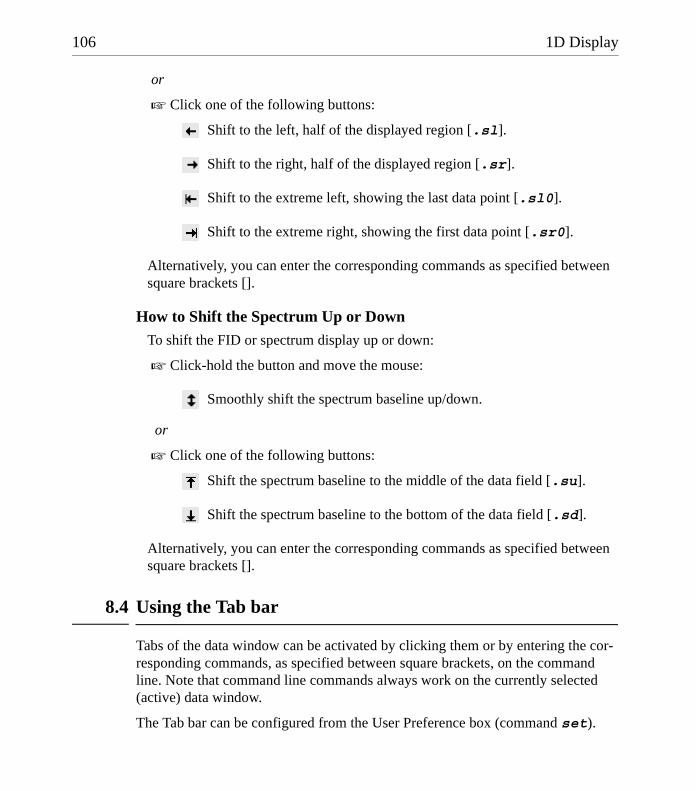
106 1D Display
DONE
INDEX
INDEX
or
! Click one of the following buttons:
Shift to the left, half of the displayed region [.sl].
Shift to the right, half of the displayed region [.sr].
Shift to the extreme left, showing the last data point [.sl0].
Shift to the extreme right, showing the first data point [.sr0].
Alternatively, you can enter the corresponding commands as specified between square brackets [].
How to Shift the Spectrum Up or DownTo shift the FID or spectrum display up or down:
! Click-hold the button and move the mouse:
Smoothly shift the spectrum baseline up/down.
or
! Click one of the following buttons:
Shift the spectrum baseline to the middle of the data field [.su].
Shift the spectrum baseline to the bottom of the data field [.sd].
Alternatively, you can enter the corresponding commands as specified between square brackets [].
8.4 Using the Tab bar
Tabs of the data window can be activated by clicking them or by entering the cor-responding commands, as specified between square brackets, on the command line. Note that command line commands always work on the currently selected (active) data window.
The Tab bar can be configured from the User Preference box (command set).
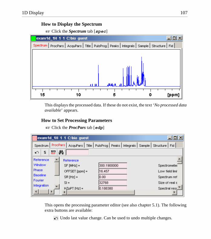
1D Display 107
DONE
INDEX
INDEX
How to Display the Spectrum
! Click the Spectrum tab [spec]
This displays the processed data. If these do not exist, the text ‘No processed data available’ appears.
How to Set Processing Parameters ! Click the ProcPars tab [edp]
This opens the processing parameter editor (see also chapter 5.1). The following extra buttons are available:
Undo last value change. Can be used to undo multiple changes.
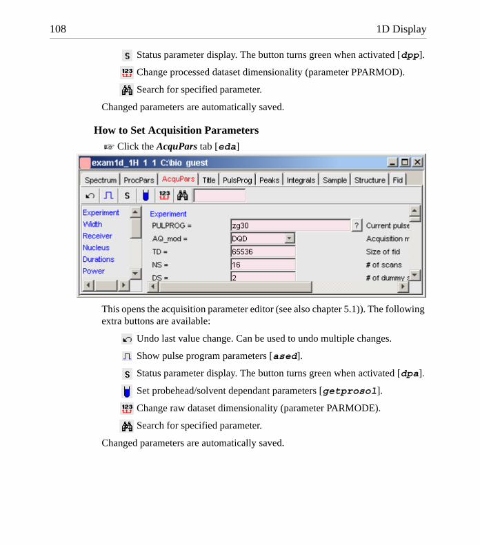
108 1D Display
DONE
INDEX
INDEX
Status parameter display. The button turns green when activated [dpp].
Change processed dataset dimensionality (parameter PPARMOD).
Search for specified parameter.
Changed parameters are automatically saved.
How to Set Acquisition Parameters ! Click the AcquPars tab [eda]
This opens the acquisition parameter editor (see also chapter 5.1)). The following extra buttons are available:
Undo last value change. Can be used to undo multiple changes.
Show pulse program parameters [ased].
Status parameter display. The button turns green when activated [dpa].
Set probehead/solvent dependant parameters [getprosol].
Change raw dataset dimensionality (parameter PARMODE).
Search for specified parameter.
Changed parameters are automatically saved.
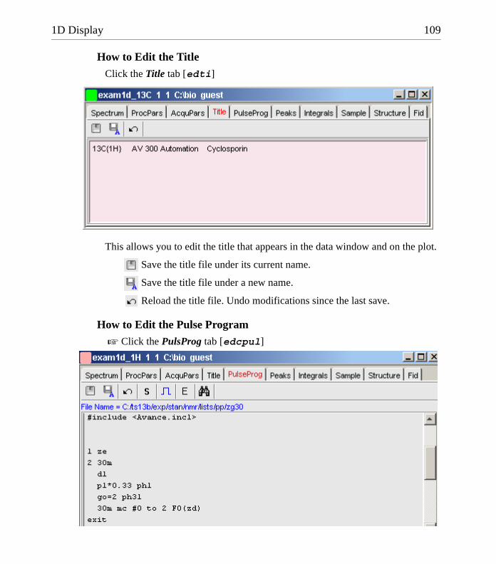
1D Display 109
DONE
INDEX
INDEX
How to Edit the Title
Click the Title tab [edti]
This allows you to edit the title that appears in the data window and on the plot.
Save the title file under its current name.
Save the title file under a new name.
Reload the title file. Undo modifications since the last save.
How to Edit the Pulse Program ! Click the PulsProg tab [edcpul]
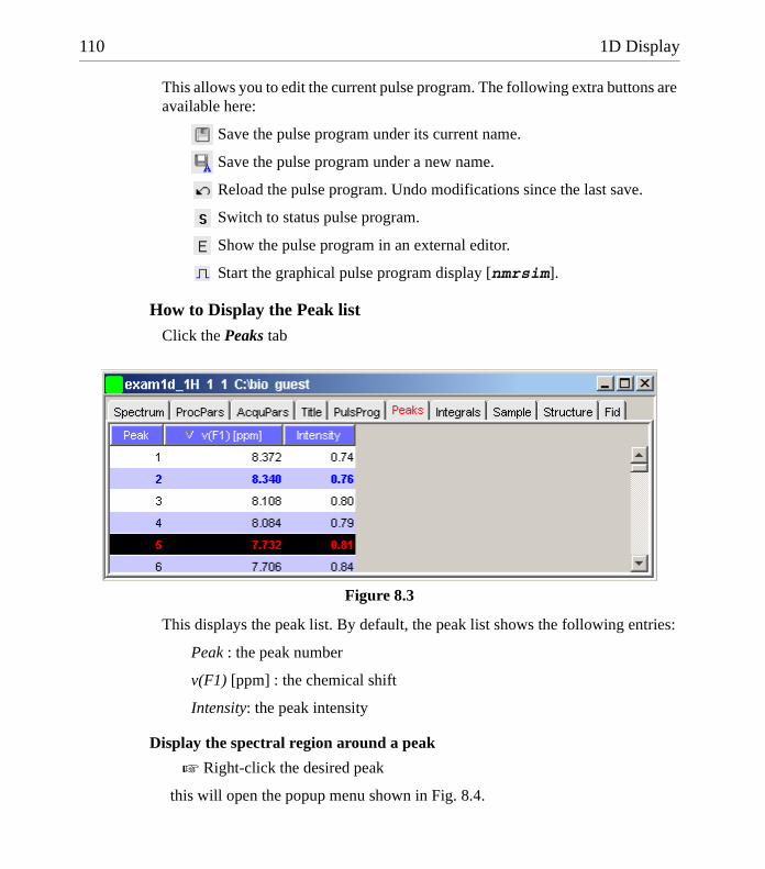
110 1D Display
DONE
INDEX
INDEX
This allows you to edit the current pulse program. The following extra buttons are available here:
Save the pulse program under its current name.
Save the pulse program under a new name.
Reload the pulse program. Undo modifications since the last save.
Switch to status pulse program.
Show the pulse program in an external editor.
Start the graphical pulse program display [nmrsim].
How to Display the Peak listClick the Peaks tab
This displays the peak list. By default, the peak list shows the following entries:
Peak : the peak number
v(F1) [ppm] : the chemical shift
Intensity: the peak intensity
Display the spectral region around a peak
! Right-click the desired peak
this will open the popup menu shown in Fig. 8.4.
Figure 8.3

1D Display 111
DONE
INDEX
INDEX
Here you can choose from the following options:
! Show spectrum " In correlated window to open a new data window showing the full correlated spectrum
! Expand spectrum " In current windowto change the current data window to spectrum display, showing the region around the selected peak
! Expand spectrum " In correlated windowto open a new data window showing the region around the selected peak
Export entries of the peak list
Entries of the peak list can easily be exported to Excel or any other program as follows:
1. For multiple peaks:
Select the desired entries while pressing the Ctrl or Shift key
2. Right-click an entry to open the popup menu (see Fig. 8.4)
3. Click one of the following menu items:
• Copy Copy the selected peak(s) entry to the Clipboard. Equivalent to click-ing Edit " Copy or hitting Ctrl+c. Copied peaks can easily be pasted in any other application such as Excel.
Figure 8.4

112 1D Display
DONE
INDEX
INDEX
• Export...Export selected peaks. Opens a dialog box where you can specify the export file (.cvs, .txt or .xml). Check the box in the lower-left corner to export the selected peaks only or uncheck it to export the entire list. Then click Export.
Import a peak List
A peak list from a different dataset can be imported as follows:
1. Right-click an entry to open the popup menu (see Fig. 8.4)
2. Click Import...
3. In the appearing dialog box, navigate to the directory where the list resides and select the peak list (.xml or .txt).
As such you can import a peak list from a different dataset or a previously ex-ported list from the current dataset. Note that peak picking commands store the peak list in the processed data directory under the name peak.txt.
Delete/remove peaks from the peak list
To delete one peak:
! Right-click the peak and choose Delete from the popup menu
To delete multiple peaks:
1. Select the peaks while pressing the Ctrl or Shift key
2. Right-click one of the peaks and choose Delete from the popup menu
To remove possible duplicate peaks:
! Right-click any entry and choose Remove " Duplicate peaks
To remove possible peaks outside of the spectrum:
! Right-click any entry and choose Remove " Peaks positioned outside of the spectrum
Shortcuts
Double-click a peak : zoom into spectrum, i.e. show region around that peak
Enter key : zoom into spectrum, i.e. show region around selected peak(s))
Delete key : delete the selected peak(s) from the peak list

1D Display 113
DONE
INDEX
INDEX
Ctrl+c : copy selected peaks to the Clipboard.
Ctrl+a : select all peaks.
Home : select the first peak
End : select the last peak.
Shift+Home : select current and first peak and all in between.
Shift+End : select current and last peak and all in between.
Note that these keys only work when the cursor focus is in the data window.
More features
The right-click popup menu has the following entries (see Fig. 8.4):
Table propertiesSet the shown columns and specify their decimal places.
Show detailed informationShow peak information, dataset information and peak picking parameters.
When you move the cursor over the peak list, the active peak will be highlighted in blue (see peak 3 in Fig. 8.5). If the correlated spectrum is also displayed, a vertical line moves along, showing corresponding position in the spectrum (see Fig. 8.5)
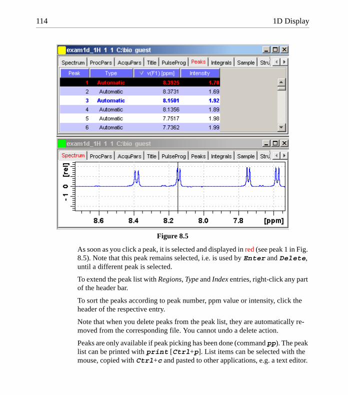
114 1D Display
DONE
INDEX
INDEX
As soon as you click a peak, it is selected and displayed in red (see peak 1 in Fig. 8.5). Note that this peak remains selected, i.e. is used by Enter and Delete, until a different peak is selected.
To extend the peak list with Regions, Type and Index entries, right-click any part of the header bar.
To sort the peaks according to peak number, ppm value or intensity, click the header of the respective entry.
Note that when you delete peaks from the peak list, they are automatically re-moved from the corresponding file. You cannot undo a delete action.
Peaks are only available if peak picking has been done (command pp). The peak list can be printed with print [Ctrl+p]. List items can be selected with the mouse, copied with Ctrl+c and pasted to other applications, e.g. a text editor.
Figure 8.5
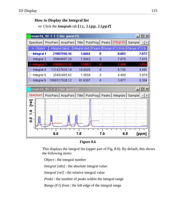
1D Display 115
DONE
INDEX
INDEX
How to Display the Integral list
! Click the Integrals tab [li, lipp, lippf]
This displays the integral list (upper part of Fig. 8.6). By default, this shows the following items:
Object : the integral number
Integral [abs] : the absolute integral value
Integral [rel] : the relative integral value
Peaks : the number of peaks within the integral range
Range (F1) from : the left edge of the integral range
Figure 8.6
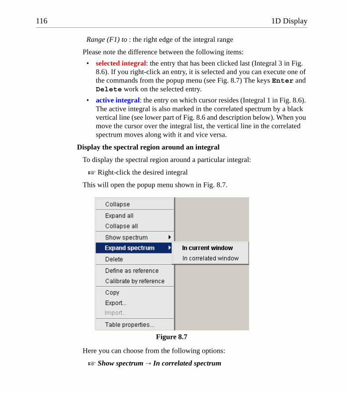
116 1D Display
DONE
INDEX
INDEX
Range (F1) to : the right edge of the integral range
Please note the difference between the following items:
• selected integral: the entry that has been clicked last (Integral 3 in Fig. 8.6). If you right-click an entry, it is selected and you can execute one of the commands from the popup menu (see Fig. 8.7) The keys Enter and Delete work on the selected entry.
• active integral: the entry on which cursor resides (Integral 1 in Fig. 8.6). The active integral is also marked in the correlated spectrum by a black vertical line (see lower part of Fig. 8.6 and description below). When you move the cursor over the integral list, the vertical line in the correlated spectrum moves along with it and vice versa.
Display the spectral region around an integral
To display the spectral region around a particular integral:
! Right-click the desired integral
This will open the popup menu shown in Fig. 8.7.
Here you can choose from the following options:
! Show spectrum " In correlated spectrum
Figure 8.7
1D Display 117
DONE
INDEX
INDEX
to open a new data window showing the full correlated spectrum
! Expand spectrum " In current windowto change the current data window to spectrum display, showing the re-gion around the selected integral
! Expand spectrum " In correlated windowto open a new data window showing the region around the selected inte-gral (lower part of Fig. 8.6)
Note that clicking the marked entry in the right-click popup menu is equivalent to pressing of the Enter key.
Export/Import Entries of the Integral List
Entries of the integral list can easily be exported to Excel or any other program as follows:
1. For multiple integrals:
Select the desired entries while pressing the Ctrl or Shift key
2. Right-click an entry to open the popup menu (see Fig. 8.7)
3. Click one of the following menu items:
• Copy Copy the selected integral(s) entry to the Clipboard. Equivalent to clicking Edit " Copy or hitting Ctrl+c. Copied integrals can easily be pasted in any other application such as Excel.
• Export...Export selected integrals. Check the box in the lower-left corner to export the selected integrals only or uncheck it to export the entire list. Then click Export.
TOPSPIN 1.3 supports exporting 1D integrals in .csv format. Future version will also 1D exporting integrals in .txt format and importing 1D integrals. These features are already supported for 2D and 3D integrals.
Calibrate Integrals to Compare Spectra
Integrals from the current and other spectra can be calibrated with respect to a reference integral. To do that:
1. Right-click the reference integral and choose Define as reference fromthe popup menu. This will determine the calibration constant.

118 1D Display
DONE
INDEX
INDEX
2. Right-click any integral and choose Calibrate by reference This will divide all integrals by the calibration constant, setting the refer-ence integral to 1.0.
Now you can read any other spectrum, and calibrate its integrals with respect to the reference integral defined above. To do that:
1. Read the spectrum
2. Enter int to define the integral ranges (if this has not been done yet)
3. Click the Integrals tab
4. Right-click any integral in the list and choose Calibrate by reference from the popup menu.
Note that the calibration constant is lost when TOPSPIN is restarted.
Display the integral list with peaks
The integral list in Fig. 8.6 shows only integrals. However, if peak picking has been done, the integral list also shows the peaks within each integral range (see Fig. 8.8).
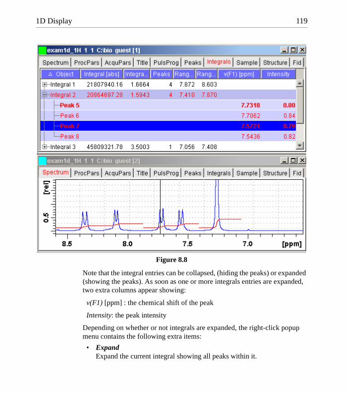
1D Display 119
DONE
INDEX
INDEX
Note that the integral entries can be collapsed, (hiding the peaks) or expanded (showing the peaks). As soon as one or more integrals entries are expanded, two extra columns appear showing:
v(F1) [ppm] : the chemical shift of the peak
Intensity: the peak intensity
Depending on whether or not integrals are expanded, the right-click popup menu contains the following extra items:
• ExpandExpand the current integral showing all peaks within it.
Figure 8.8
120 1D Display
DONE
INDEX
INDEX
• Expand allExpand all integrals showing all peaks within them.
• Collapse all Collapse all integrals hiding all peaks within them.
In addition to the integral entry, an individual peak within an integral can be activated (by placing the cursor on it) or selected (by clicking it). In Fig. 8.8, peak 7 is selected and the correlated spectrum is displayed. Peak 5 is active which is also shown by the vertical line in the correlated spectrum.
Delete an Integral from the Integral List
To delete one integral:
! Right-click the integral and choose Delete from the popup menu
To delete multiple integrals:
1. Select the integrals while pressing the Ctrl or Shift key
2. Right-click one of the integrals and choose Delete from the popup menu
Shortcuts
Enter key : zoom into spectrum, i.e. show region around selected inte-gral(s))
Delete key : delete the selected integral(s) from the integral list
Ctrl+c : copy selected integrals to the Clipboard.
Ctrl+a : select all peaks.
Home : select the first peak
End : select the last peak
Shift+Home : select current and first peak and all in between
Shift+End : select current and last peak and all in between
Double-clicking an integral will show the peaks within the integral region if they exist. It they do not exist, it will zoom into spectrum showing the inte-gral region.
Note that these keys only work when the cursor focus is in the data window.
More features

1D Display 121
DONE
INDEX
INDEX
The right-click popup menu has the following extra entry:
Table properties to set the shown columns and specify their decimal places
How to view Sample Information
! Click the Sample tab
This table can be used to fill out any sample information you want to store with the dataset. The table can easily be modified or extended with the following func-tions:
To select an item: double-click it!
Save the sample information table with the dataset.
Save the sample information table as default.
Reload the original table discarding any changes
Add a new item to the table. You will be prompted for an identification name and the desired number of lines
Figure 8.9

122 1D Display
DONE
INDEX
INDEX
Remove the selected item from the table
Move the selected item one place up in the table
Move the selected item one place down in the table
How to Open the Jmol Molecule Structure Viewer
! Click the Structure tab [jmol]:
opens the Jmol molecule structure viewer. TOPSPIN 1.3 contains Jmol version 10. This has the following features:
• The viewer displays the structure file that resides in the expno of the current dataset. If this does not exist, the structure file defined by the acquisition parameter CHEMSTR is displayed. CHEMSTR can define a full pathname or a filename. In the latter case, the file is searched for in the directory defined in the User Preferences. To set this directory, click Options " Pref-erences, select Directory pathnames, enter a directory and click OK. If no structure file is found, you can open one by clicking File " Open in the Molecule Viewer
Figure 8.10

1D Display 123
DONE
INDEX
INDEX
• The following structure file types are supported: .xyz, .mol, .pdb, .cml, .out, .mmlgp, .res, .cif, .gpr, .hin, .nwo.
• Secondary structure elements of proteins (backbone, cartoons, ribbons, ...) can be displayed in selectable sizes and colors.
• Mouse button effects:
Rotate a molecule around the x- and y-axis by pressing the left mouse button, and moving the mouse left/right or up/down, respectively.
Rotate a molecule around the z-axis by pressing the middle mouse button and moving the mouse left/right .
Zoom in or out a molecule by pressing the middle mouse button, and moving the mouse up or down.
• RASmol command scripts are supported. To send a RASmol command to the currently displayed molecule enter:
!jmol <RASmol command>
Here are some example:
!jmol zoom 400
!jmol ribbon 200
!jmol color ribbon yellow
You may create TOPSPIN macros containing RASmol commands. Just enter edmac on the TOPSPIN command line and insert the RASmol commands in the appearing editor. Here is an example:
jmol load /mystructures/alphahelix.pdb # load a structurejmol backbone 0.7 # display its backbone with 0.7 Angstrom sizejmol color backbone yellow # change backbone colorjmol background green # change background colorjmol zoom 200 # zoom structure
The available RASmol commands are described in the Jmol Help menu.
• Multiple molecules (or multiple aspects of one molecule) can be displayed simultaneously. To do that just open multiple data sets or open the same dataset in multiple data windows and click on the Structure Tab in each window.
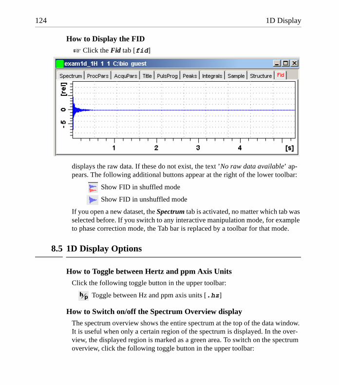
124 1D Display
DONE
INDEX
INDEX
How to Display the FID
! Click the Fid tab [fid]
displays the raw data. If these do not exist, the text ’No raw data available’ ap-pears. The following additional buttons appear at the right of the lower toolbar:
Show FID in shuffled mode
Show FID in unshuffled mode
If you open a new dataset, the Spectrum tab is activated, no matter which tab was selected before. If you switch to any interactive manipulation mode, for example to phase correction mode, the Tab bar is replaced by a toolbar for that mode.
8.5 1D Display Options
How to Toggle between Hertz and ppm Axis Units
Click the following toggle button in the upper toolbar:
Toggle between Hz and ppm axis units [.hz]
How to Switch on/off the Spectrum Overview display
The spectrum overview shows the entire spectrum at the top of the data window. It is useful when only a certain region of the spectrum is displayed. In the over-view, the displayed region is marked as a green area. To switch on the spectrum overview, click the following toggle button in the upper toolbar:

1D Display 125
DONE
INDEX
INDEX
Switch the spectrum overview display on/off [.ov]
To shift the displayed region, simply click-hold the green area in the overview spectrum and move the mouse (see Fig. 8.11).
How to Switch Y-axis Display Click the following toggle button in the upper toolbar:
Switch the y-axis display between abs/rel/off [.y]
Fig. 8.11 shows a data window with the spectrum overview on, ppm axis units, and absolute y-axis display.
Figure 8.11
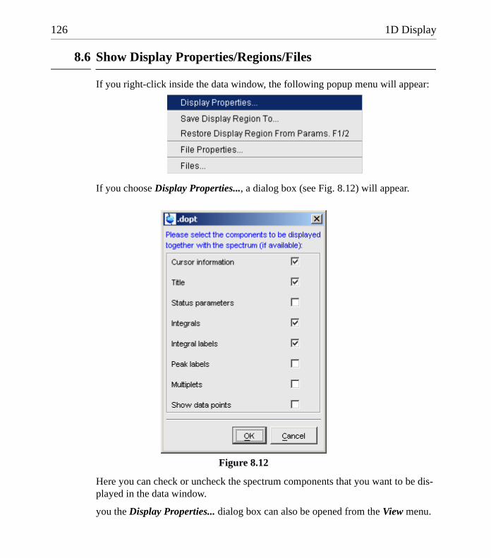
126 1D Display
DONE
INDEX
INDEX
8.6 Show Display Properties/Regions/Files
If you right-click inside the data window, the following popup menu will appear:
If you choose Display Properties..., a dialog box (see Fig. 8.12) will appear.
Here you can check or uncheck the spectrum components that you want to be dis-played in the data window.
you the Display Properties... dialog box can also be opened from the View menu.
Figure 8.12
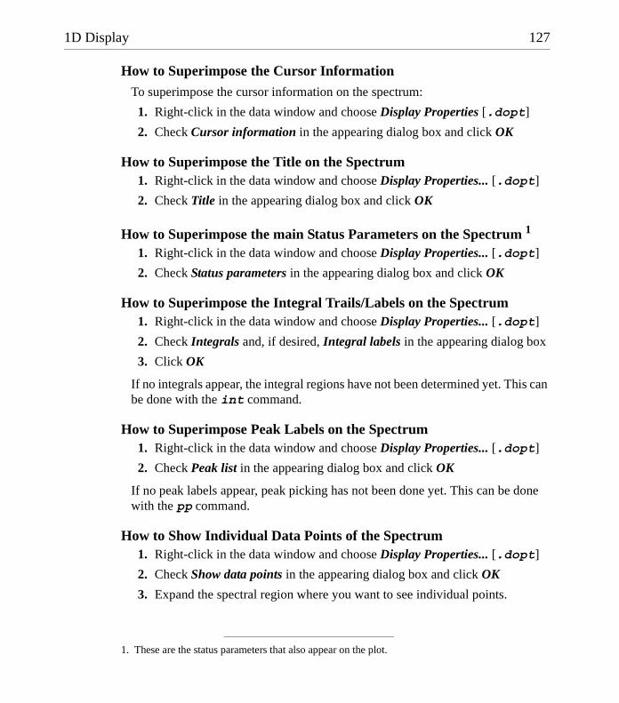
1D Display 127
DONE
INDEX
INDEX
How to Superimpose the Cursor Information
To superimpose the cursor information on the spectrum:
1. Right-click in the data window and choose Display Properties [.dopt]
2. Check Cursor information in the appearing dialog box and click OK
How to Superimpose the Title on the Spectrum1. Right-click in the data window and choose Display Properties... [.dopt]
2. Check Title in the appearing dialog box and click OK
How to Superimpose the main Status Parameters on the Spectrum 1
1. Right-click in the data window and choose Display Properties... [.dopt]
2. Check Status parameters in the appearing dialog box and click OK
How to Superimpose the Integral Trails/Labels on the Spectrum1. Right-click in the data window and choose Display Properties... [.dopt]
2. Check Integrals and, if desired, Integral labels in the appearing dialog box
3. Click OK
If no integrals appear, the integral regions have not been determined yet. This can be done with the int command.
How to Superimpose Peak Labels on the Spectrum1. Right-click in the data window and choose Display Properties... [.dopt]
2. Check Peak list in the appearing dialog box and click OK
If no peak labels appear, peak picking has not been done yet. This can be done with the pp command.
How to Show Individual Data Points of the Spectrum1. Right-click in the data window and choose Display Properties... [.dopt]
2. Check Show data points in the appearing dialog box and click OK
3. Expand the spectral region where you want to see individual points.
1. These are the status parameters that also appear on the plot.

128 1D Display
DONE
INDEX
INDEX
How to Display the Main Dataset Properties
! Right-click inside the data window and choose File Properties
An information box as displayed in Fig. 8.13 will appear.
Note that this is status information which cannot be changed.
How to Display a List of Files of a Dataset! Right-click inside the data window choose Files
Fig. 8.14 shows the file list when the Fid tab is active, i.e. when the raw data are displayed. It is the contents of the expno directory.
Figure 8.13
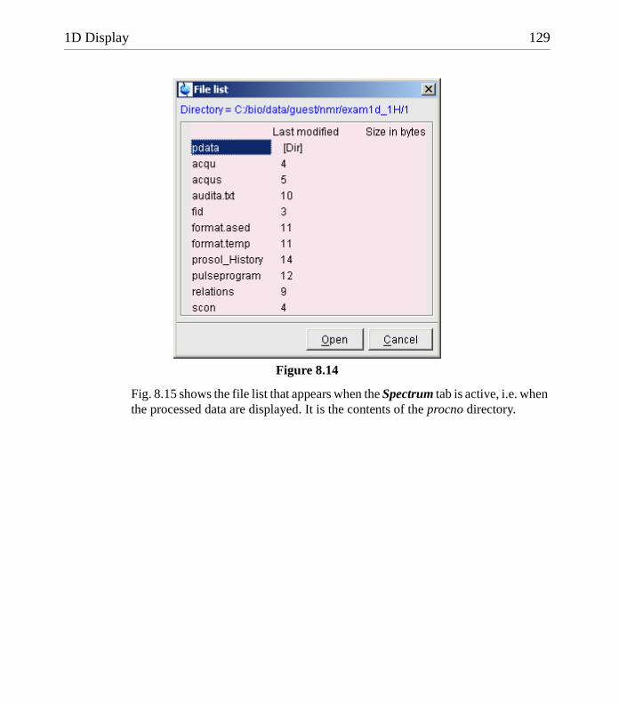
1D Display 129
DONE
INDEX
INDEX
Fig. 8.15 shows the file list that appears when the Spectrum tab is active, i.e. when the processed data are displayed. It is the contents of the procno directory.
Figure 8.14

130 1D Display
DONE
INDEX
INDEX
The contents of any file in the list can be displayed as follows:
1. Select a filename (it will be highlighted)
2. Click Open
Note that this only makes sense for ascii files, e.g. acqu*, proc* or files with the extension .txt.
Dataset files can also be displayed/opened with the command expl. This opens the Windows Explorer, or under Linux, the Konqueror or Mozilla, showing the contents of the procno directory.
8.7 Saving Display Region
The currently displayed spectral region can be stored as follows:
! Right-click in the data window and choose Save Display Region To...
Figure 8.15
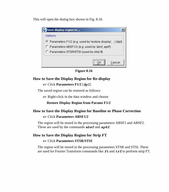
This will open the dialog box shown in Fig. 8.16.
How to Save the Display Region for Re-display! Click Parameters F1/2 [dpl]
The saved region can be restored as follows:
! Right-click in the data window and choose
Restore Display Region from Params F1/2
How to Save the Display Region for Baseline or Phase Correction! Click Parameters ABSF1/2
The region will be stored in the processing parameters ABSF1 and ABSF2. These are used by the commands absf and apkf.
How to Save the Display Region for Strip FT! Click Parameters STSR/STSI
The region will be stored in the processing parameters STSR and STSI. These are used for Fourier Transform commands like ft and trf to perform strip FT.
Figure 8.16


Chapter 9
2D Display
9.1 The 2D Data Window
The 2D data window consists of a data field, a title bar, a Tab bar and buttons.
Fig. 9.1 shows a data window with a 2D spectrum.
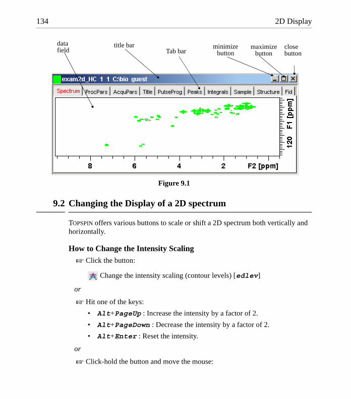
134 2D Display
DONE
INDEX
INDEX
.
9.2 Changing the Display of a 2D spectrum
TOPSPIN offers various buttons to scale or shift a 2D spectrum both vertically and horizontally.
How to Change the Intensity Scaling
! Click the button:
Change the intensity scaling (contour levels) [edlev]
or
! Hit one of the keys:
• Alt+PageUp : Increase the intensity by a factor of 2.
• Alt+PageDown : Decrease the intensity by a factor of 2.
• Alt+Enter : Reset the intensity.
or
! Click-hold the button and move the mouse:
Figure 9.1
Tab bar data field minimize
button maximize
button closebutton
title bar

2D Display 135
DONE
INDEX
INDEX
Increase/decrease the intensity smoothly.
or
! Click one of the following buttons:
Increase the intensity (decrease the levels) by 2 [*2].
Increase the intensity (decrease the levels) by 8 [*8].
Decrease the intensity (increase the levels) by 2 [/2].
Decrease the intensity (increase the levels) by 8 [/8].
Reset the intensity to the last saved intensity (contour levels) [.vr].
Alternatively, you can enter the corresponding commands as specified between square brackets [].
To manipulate all data windows, press the Ctrl key while clicking one of the above buttons.
How to Switch on/off Square 2D layout
Right-click inside the data field and click Square Layout On/Off

136 2D Display
DONE
INDEX
INDEX
The F2 scaling will be adjusted to reach a square display.
How to Zoom a 2D spectrum in/out! Click one of the following buttons:
Zoom in [.zi].
Zoom out [.zo].
Perform an exact zoom via a dialog box [.zx].
a) Enter the coordinates of the desired region in the dialog box.
Figure 9.2
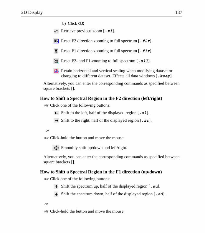
2D Display 137
DONE
INDEX
INDEX
b) Click OK
Retrieve previous zoom [.zl].
Reset F2 direction zooming to full spectrum [.f2r].
Reset F1 direction zooming to full spectrum [.f1r].
Reset F2- and F1-zooming to full spectrum [.all].
Retain horizontal and vertical scaling when modifying dataset or changing to different dataset. Effects all data windows [.keep].
Alternatively, you can enter the corresponding commands as specified between square brackets [].
How to Shift a Spectral Region in the F2 direction (left/right)! Click one of the following buttons:
Shift to the left, half of the displayed region [.sl].
Shift to the right, half of the displayed region [.sr].
or
! Click-hold the button and move the mouse:
Smoothly shift up/down and left/right.
Alternatively, you can enter the corresponding commands as specified between square brackets [].
How to Shift a Spectral Region in the F1 direction (up/down)
! Click one of the following buttons:
Shift the spectrum up, half of the displayed region [.su].
Shift the spectrum down, half of the displayed region [.sd].
or
! Click-hold the button and move the mouse:
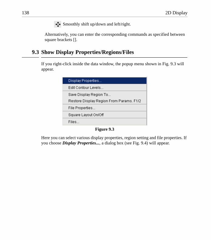
138 2D Display
DONE
INDEX
INDEX
Smoothly shift up/down and left/right.
Alternatively, you can enter the corresponding commands as specified between square brackets [].
9.3 Show Display Properties/Regions/Files
If you right-click inside the data window, the popup menu shown in Fig. 9.3 will appear.
Here you can select various display properties, region setting and file properties. If you choose Display Properties..., a dialog box (see Fig. 9.4) will appear.
Figure 9.3

2D Display 139
DONE
INDEX
INDEX
Here you can set various display options including parameter, integrals, peaks, contours and projections.
9.4 Using the Tab bar
The 2D data window is a tabbed pane. This means its contents depends on the cur-rently active tab in the Tab bar. The individual tabs are basically the same as for 1D display (see chapter 8.4). There are, however, some differences, which are dis-cussed below.
Figure 9.4
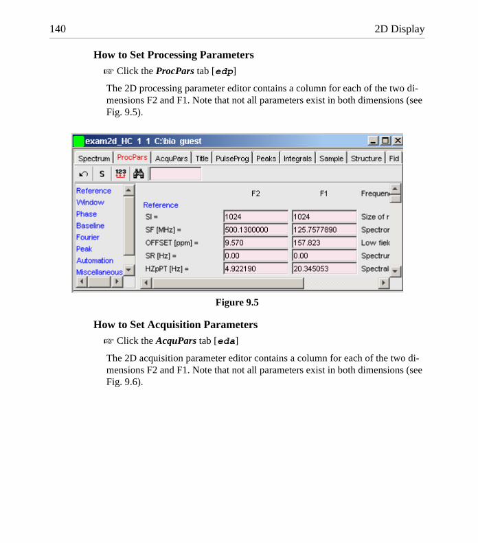
140 2D Display
DONE
INDEX
INDEX
How to Set Processing Parameters
! Click the ProcPars tab [edp]
The 2D processing parameter editor contains a column for each of the two di-mensions F2 and F1. Note that not all parameters exist in both dimensions (see Fig. 9.5).
How to Set Acquisition Parameters ! Click the AcquPars tab [eda]
The 2D acquisition parameter editor contains a column for each of the two di-mensions F2 and F1. Note that not all parameters exist in both dimensions (see Fig. 9.6).
Figure 9.5
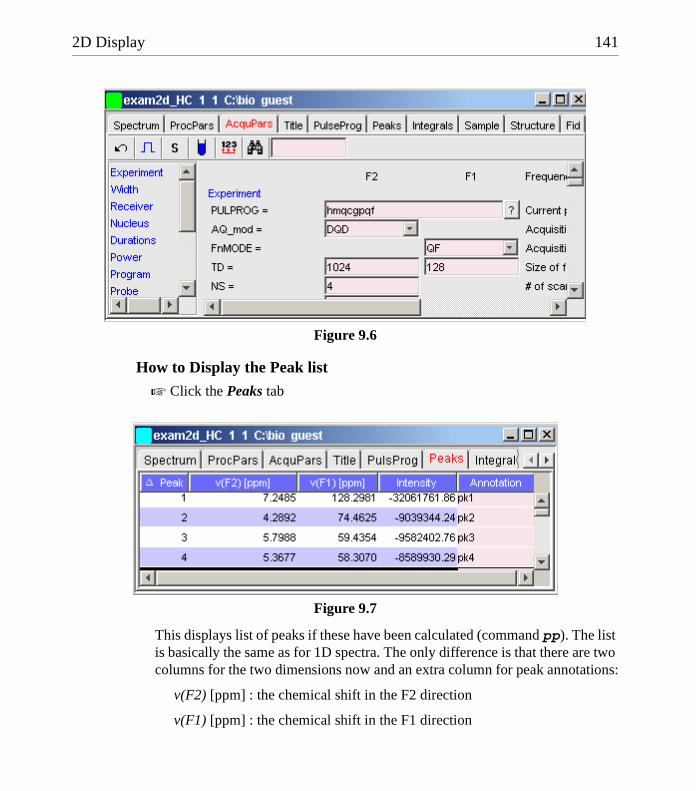
2D Display 141
DONE
INDEX
INDEX
How to Display the Peak list
! Click the Peaks tab
This displays list of peaks if these have been calculated (command pp). The list is basically the same as for 1D spectra. The only difference is that there are two columns for the two dimensions now and an extra column for peak annotations:
v(F2) [ppm] : the chemical shift in the F2 direction
v(F1) [ppm] : the chemical shift in the F1 direction
Figure 9.6
Figure 9.7

142 2D Display
DONE
INDEX
INDEX
Annotation: the peak annotation
To specify or edit an annotation, click inside the Annotation field and enter a character string. The peak annotations are shown in the correlated spectrum (see Fig. 9.8)
How to Display the Integral list
! Click the Integrals tab
Figure 9.8

2D Display 143
DONE
INDEX
INDEX
This displays list of integrals if these have been calculated (command int). The list is basically the same as for 1D spectra. The only difference is that, when peaks are shown, there are two columns for the chemical shift:
v(F2) [ppm] : the chemical shift in the F2 direction
v(F1) [ppm] : the chemical shift in the F1 direction
Furthermore, a stored or exported 2D integral list can be imported as follows:
1. Right-click an entry to open the popup menu
2. Click Import...
3. In the appearing dialog box, navigate to the directory where the list resides and select the integral list.
As such you can import an integral list from a different dataset or a previously exported list from the current dataset. Note that integration commands store the integral list in the processed data directory under the name inte-grals.txt. Exported integrals are stored in the files <name>.txt and <name>.reg, where <name> is the name specified by the user.
How to Display the FID ! Click the Fid tab [fid]
Figure 9.9
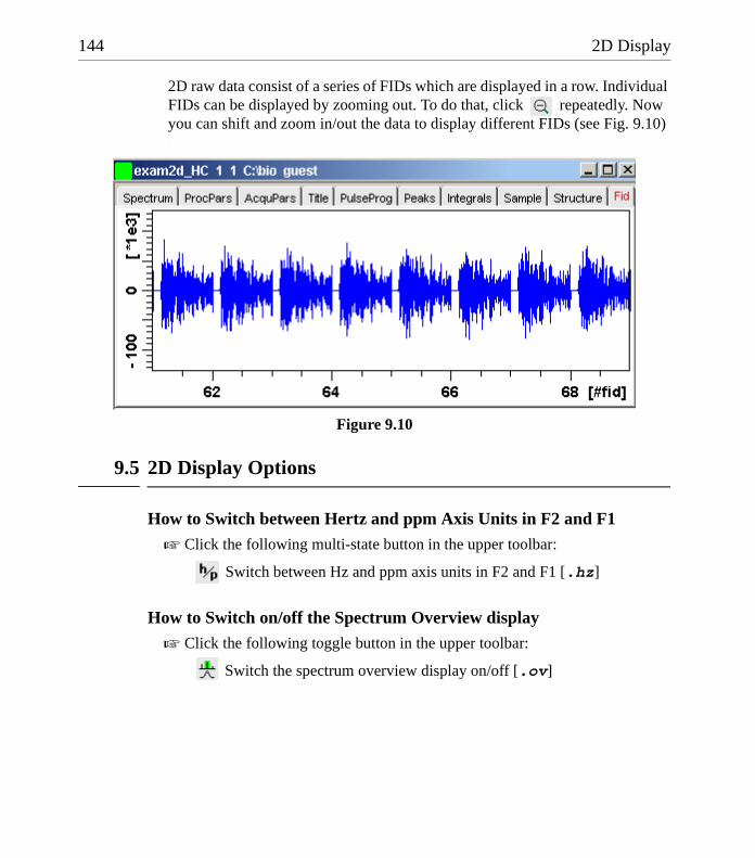
144 2D Display
DONE
INDEX
INDEX
2D raw data consist of a series of FIDs which are displayed in a row. Individual FIDs can be displayed by zooming out. To do that, click repeatedly. Now you can shift and zoom in/out the data to display different FIDs (see Fig. 9.10) .
9.5 2D Display Options
How to Switch between Hertz and ppm Axis Units in F2 and F1! Click the following multi-state button in the upper toolbar:
Switch between Hz and ppm axis units in F2 and F1 [.hz]
How to Switch on/off the Spectrum Overview display! Click the following toggle button in the upper toolbar:
Switch the spectrum overview display on/off [.ov]
Figure 9.10

2D Display 145
DONE
INDEX
INDEX
With the spectrum overview on, the data window will, for example, look like this:
How to Switch on/off the Projection display! Click the following toggle button in the upper toolbar:
Switch the projection display on/off [.pr]
With the projections displayed, a 2D dataset looks like this:
In this example, the F1 projection is selected as indicated by the filled blue square

146 2D Display
DONE
INDEX
INDEX
whereas the F2 projection is not selected. A selected projection can be rescaled using the toolbar rescale buttons of function keys. If you right-click inside the pro-jection area of the data window, the following popup menu appears:
Clicking External Projection opens the a dialog box where you can specify or search for a 1D dataset and display this as a projection of the current 2D dataset.
Clicking Internal Projection calculates and displays the positive projection and displays it along with the 2D spectrum.
Clicking Baseline at Bottom or Baseline at Center allows you to put the projec-tion baseline at the respective positions.
Various other projection features are available. To access them:
click Processing " Calculate projections [proj]
This will open the dialog box shown in Fig. 9.11.
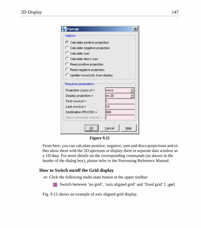
2D Display 147
DONE
INDEX
INDEX
From here, you can calculate positive, negative, sum and disco projections and ei-ther show them with the 2D spectrum or display them in separate data window as a 1D data. For more details on the corresponding commands (as shown in the header of the dialog box), please refer to the Processing Reference Manual.
How to Switch on/off the Grid display
! Click the following multi-state button in the upper toolbar:
Switch between ’no grid’, ’axis aligned grid’ and ’fixed grid’ [.gr]
Fig. 9.12 shows an example of axis aligned grid display.
Figure 9.11

148 2D Display
DONE
INDEX
INDEX
How to Display a 2D Spectrum in Contour Mode
! Click the following button in the upper toolbar:
Switch to contour display mode [.co]
In contour mode, a spectral region looks like this:
Figure 9.12 Axis aligned grid display

2D Display 149
DONE
INDEX
INDEX
How to Set the 2D Contour Levels
! Click the following button in the lower toolbar
Edit contour levels [edlev, .lv]
This will open the following dialog box shown in Fig. 9.13. Contour levels can be entered manually or they can be calculated.
Manual setup
This allows you to create an arbitrary sequence of levels
1. Enter the level values in the fields 1, 2, ... at the top of the dialog box.
2. Click Apply to update the display or OK to store the levels, update the display and close the dialog box.
Calculation
This allows you to easily create a geometric or equidistant sequence of levels.
1. Click one of the following items:
• Multiply with increment to create a geometric sequence of levels.
• Add incrementto create a equidistant sequence of levels.
2. Enter the desired Base level, Level increment and Number of levels.
3. Click Fill to display and activate the sequence.
4. Click Apply to update the display or OK to store the levels, update the display and close the dialog box.
The Contour level sign allows you to select positive levels, negative levels or both.

150 2D Display
DONE
INDEX
INDEX
How to Store interactively set Contour Levels
To store contour levels that were set interactively, for example by clicking or
Figure 9.13
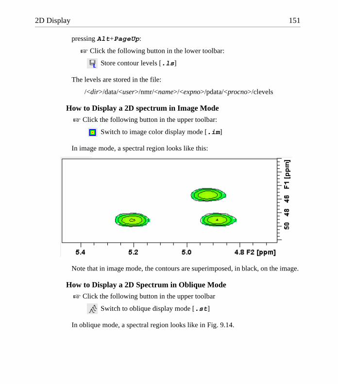
2D Display 151
DONE
INDEX
INDEX
pressing Alt+PageUp:
! Click the following button in the lower toolbar:
Store contour levels [.ls]
The levels are stored in the file:
/<dir>/data/<user>/nmr/<name>/<expno>/pdata/<procno>/clevels
How to Display a 2D spectrum in Image Mode
! Click the following button in the upper toolbar:
Switch to image color display mode [.im]
In image mode, a spectral region looks like this:
Note that in image mode, the contours are superimposed, in black, on the image.
How to Display a 2D Spectrum in Oblique Mode! Click the following button in the upper toolbar
Switch to oblique display mode [.st]
In oblique mode, a spectral region looks like in Fig. 9.14.

152 2D Display
DONE
INDEX
INDEX
In this mode you can manipulate the display in various ways. Just right-click in-side the data window and choose one of the options from the appearing popup menu (see Fig. 9.15)
Figure 9.14
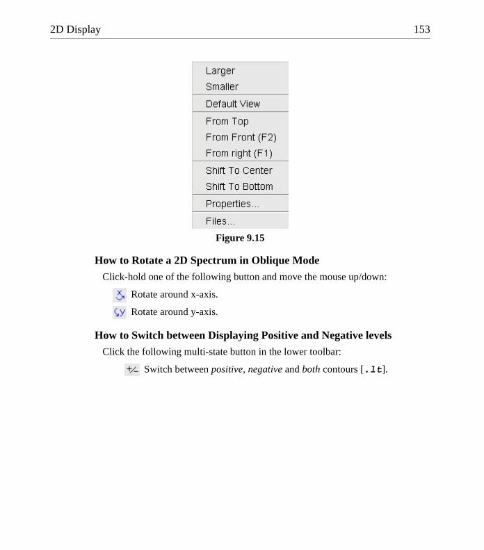
2D Display 153
DONE
INDEX
INDEX
:
How to Rotate a 2D Spectrum in Oblique Mode
Click-hold one of the following button and move the mouse up/down:
Rotate around x-axis.
Rotate around y-axis.
How to Switch between Displaying Positive and Negative levels
Click the following multi-state button in the lower toolbar:
Switch between positive, negative and both contours [.lt].
Figure 9.15

Chapter 10
3D Display
10.1 Plane Display Mode
3D data can be displayed as 2D planes or as a 3D cube. By default, the first F3-F1 plane is displayed (see Fig. 10.1) The plane orientation and number is shown. The cube in the lower left corner graphically indicates which plane is displayed. The full 2D display functionality is available (see chapter 9).

156 3D Display
DONE
INDEX
INDEX
How to Switch to 2D Plane Display
If the 3D cube is displayed you can switch to 2D plane display by clicking one of the following buttons:
Switch to 2D contour display.
Switch to 2D image display.
Switch to 2D oblique display.
How to Display various Plane Orientations
Click one of the following buttons:
Show F1-F2 planes.
Figure 10.1
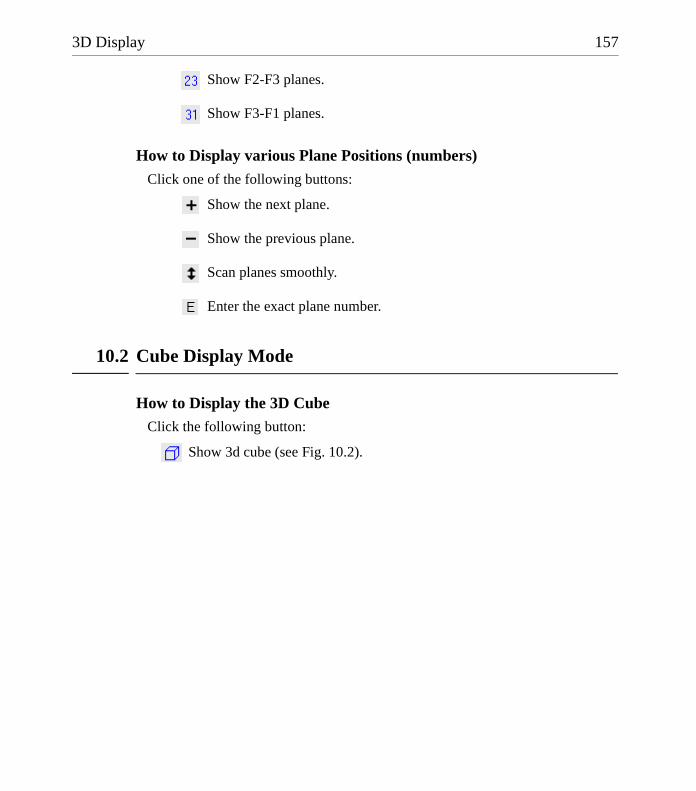
3D Display 157
DONE
INDEX
INDEX
Show F2-F3 planes.
Show F3-F1 planes.
How to Display various Plane Positions (numbers)
Click one of the following buttons:
Show the next plane.
Show the previous plane.
Scan planes smoothly.
Enter the exact plane number.
10.2 Cube Display Mode
How to Display the 3D CubeClick the following button:
Show 3d cube (see Fig. 10.2).

158 3D Display
DONE
INDEX
INDEX
How to Rotate the 3D Cube
Click-hold one the following buttons and move the mouse up/down:
Rotate cube around x-axis.
Rotate cube around y-axis.
Rotate cube around z-axis.
How to Scale Up/Down the 3D Cube1. Right-click inside the data window.
2. Choose Larger or Smaller from the popup menu (see Fig. 10.3).
How to Reset the Cube Size and Orientation
Click the following button:
Reset to default size and orientation.
Figure 10.2

3D Display 159
DONE
INDEX
INDEX
How to Switch Depth Cueing on/off1. Right-click inside the data window
2. Choose Depth Cueing On/off (see Fig. 10.3)
Depth cueing makes data points which are closer to the viewer appear brighter and those that are further away appear dimmer. This increases the depth effect of the 3D image.
How to Display a Cube Front or Side viewClick one the following buttons:
Show F1-F2 plane.
Show F2-F3 plane.
Show F3-F1 plane.
10.3 Using the Tab bar
The 3D data window is a tabbed pane. This means its contents depends on the currently active tab in the Tab bar. The individual tabs are basically the same as for 1D and 2D display (see chapter 8.4). When you click the ProcPars or AcquPars tab, you will find a parameters column for each of the three dimen-sions F3, F2 and F1. The Fid tab allows you to display the 3D raw data as a series of 1D FIDs. The Peaks tab will display the 3D peak list with a column for the chemical shift in each of the three dimensions. Similarly, the Integrals
Figure 10.3
160 3D Display
DONE
INDEX
INDEX
tab will display the 3D integral list. Peaks and integrals only appear if they have been calculated (commands pp and int, respectively).When the integral list shows peaks, with a column for the chemical shift in each of the three di-mensions appears. Like in 2D, a stored or exported 3D integral list can be im-ported (see Fig. 9.4).
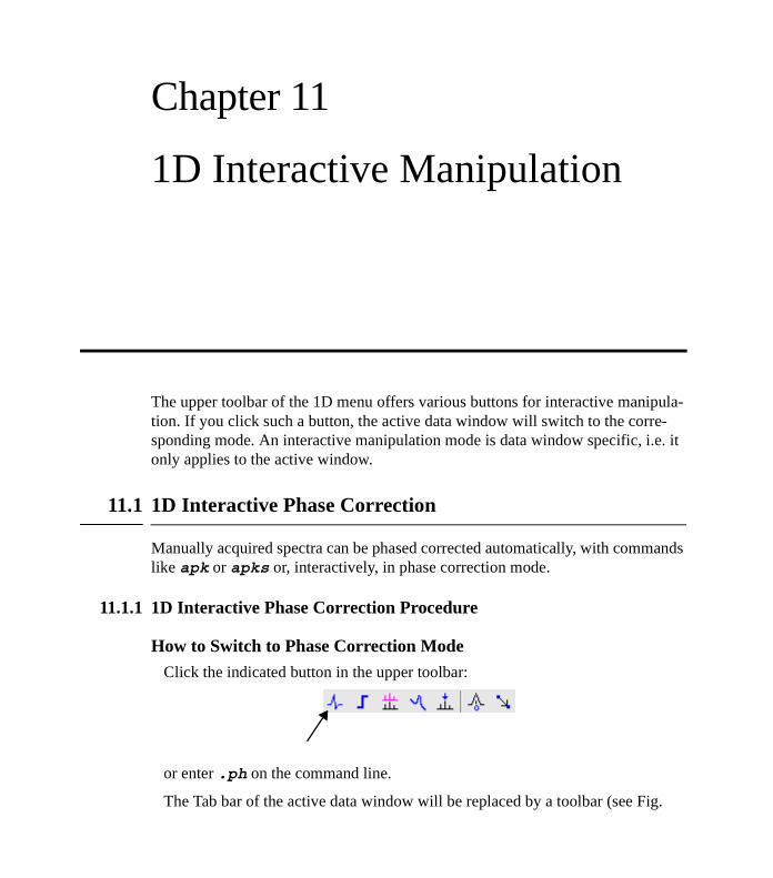
Chapter 11
1D Interactive Manipulation
The upper toolbar of the 1D menu offers various buttons for interactive manipula-tion. If you click such a button, the active data window will switch to the corre-sponding mode. An interactive manipulation mode is data window specific, i.e. it only applies to the active window.
11.1 1D Interactive Phase Correction
Manually acquired spectra can be phased corrected automatically, with commands like apk or apks or, interactively, in phase correction mode.
11.1.1 1D Interactive Phase Correction Procedure
How to Switch to Phase Correction ModeClick the indicated button in the upper toolbar:
or enter .ph on the command line.
The Tab bar of the active data window will be replaced by a toolbar (see Fig.
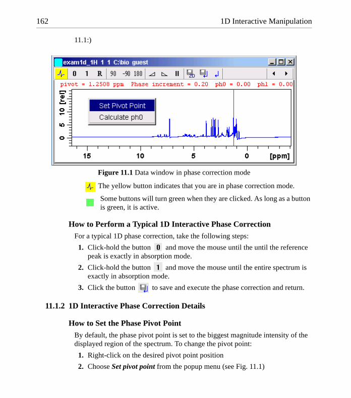
162 1D Interactive Manipulation
DONE
INDEX
INDEX
11.1:)
The yellow button indicates that you are in phase correction mode.
Some buttons will turn green when they are clicked. As long as a button is green, it is active.
How to Perform a Typical 1D Interactive Phase CorrectionFor a typical 1D phase correction, take the following steps:
1. Click-hold the button and move the mouse until the until the reference peak is exactly in absorption mode.
2. Click-hold the button and move the mouse until the entire spectrum is exactly in absorption mode.
3. Click the button to save and execute the phase correction and return.
11.1.2 1D Interactive Phase Correction Details
How to Set the Phase Pivot Point
By default, the phase pivot point is set to the biggest magnitude intensity of the displayed region of the spectrum. To change the pivot point:
1. Right-click on the desired pivot point position
2. Choose Set pivot point from the popup menu (see Fig. 11.1)
Figure 11.1 Data window in phase correction mode
1D Interactive Manipulation 163
DONE
INDEX
INDEX
How to Perform Default Zero Order Phase Correction1. Right-click in the data window
2. Choose Calculate ph0 in the popup menu (see Fig. 11.1)
The spectrum will automatically be corrected according to the calculated value.
How to Perform Interactive Zero Order Phase Correction1. Click-hold the following button (button turns green):
Zero order phase correction (parameter PHC0).
2. Move the mouse until the reference peak is exactly in absorption mode.
3. Release the mouse (button turns grey).
How to Perform Interactive First Order Phase Correction1. Click-hold the following button (button turns green):
First order phase correction (parameter PHC1).
2. Move the mouse until the entire spectrum is exactly in absorption mode.
3. Release the mouse (button turns grey).
How to Perform 90, -90 or 180° Zero Order Phase Correction ! Click one of the following buttons:
Perform 90 zero order phase correction [.ph90].
Perform -90° zero order phase correction [.phm90].
Perform 180° zero order phase correction [.ph180].
How to Reset the Phase to the Original Values! Click the following button:
Reset zero and first order phase values [.phr].
How to Change the Mouse Sensitivity ! Click one of the following buttons:
164 1D Interactive Manipulation
DONE
INDEX
INDEX
Increase (double) the mouse sensitivity [.inc].
Decrease (halve) the mouse sensitivity [.dec].
Reset the mouse sensitivity.
How to Return from Phase Correction Mode with/without Save To return while saving the phase correction to the current dataset:
! Click the following button:
Save, execute and return [.sret].
This will perform the following tasks:
• Execute phase correction (command pk).
• Save the current phase correction values.
• Leave the phase correction mode.
To return without save:
! Click the following button:
Return, discarding any changes [.ret].
To return while saving the phase correction to the source 2D dataset:
! Click the following button:
Save to 2D [.s2d].
This is only applicable on rows or columns extracted from 2D data. The phase values will be saved to the 2D dataset from which the current 1D data-set was extracted.
11.2 1D Interactive Integration
Integration of 1D data can be done automatically, with the commands abs and li or, interactively, as described in this paragraph.

1D Interactive Manipulation 165
DONE
INDEX
INDEX
How to Switch to Integration Mode
! Click the indicated button in the upper toolbar:
or enter .int on the command line.
The Tab bar of the active data window will be replaced by a toolbar (see Fig. 11.2).
The yellow button indicates that the data window is in integration mode.
Some buttons will turn green when they are clicked. As long as a button is green, it is active.
If integral regions have already been determined, for example with abs or with a previous interactive integration, these regions are displayed in the data window, along with the integral values. You can remove them, change them or add to them, as described below.
Figure 11.2 Data window in integration mode

166 1D Interactive Manipulation
DONE
INDEX
INDEX
How to Define Integral Regions
To define integral regions interactively:
1. Click the following button (button turns green):
Define integral region interactively.
2. Put the red cursor line at one edge of a peak or multiplet.
3. Left-click-hold and drag the cursor line to the other edge of the peak or mul-tiplet.
4. Do step 2 and 3 for all regions to be defined.
5. Click the green button to leave the "define region" mode (button turns grey).
To define integral regions via a dialog box:
1. Click the following button:
Define region via dialog.
2. In the appearing dialog box:
Enter the exact values for the region limits.
3. Click OK to define the selected region.
How to Select/Deselect Integral Regions
To select/deselect all displayed integral regions:
! Click the following button:
Select/Deselect all regions.
To select a single integral region:

1D Interactive Manipulation 167
DONE
INDEX
INDEX
1. Right-click in the integral region.
2. Choose Select/Deselect from the popup menu.
Selected integral regions are indicated by a color filled integral label. In the Fig. 11.3, the two left most regions have already been selected, the right most region is currently being selected.
How to Read Integral Regions from Disk
You can read integrals regions from disk which have been stored by automatic in-tegration (command abs) or by a previous interactive integration.
To read integrals:
1. Click the following button:
Read integral regions.
The following popup menu will appear:
Figure 11.3

168 1D Interactive Manipulation
DONE
INDEX
INDEX
2. From the popup menu, choose one of the following entries:
• Read ’intrng’to read the last saved integral regions and apply the saved slope and bias correction values.
• Read ’intrng’ no slope & bias corr.to read the last saved integral regions but do not apply the saved slope and bias correction values.
• Read ’intrng’ use last slope & biasto read the last saved integral regions applying the last slope and bias correction values.
• Edit ’intrng’to edit the file (intrng) that contains the integral regions and slope and bias correction values. Changes in this file are automatically shown on the screen.
How to Perform Interactive Bias and Slope CorrectionTo perform interactive bias correction:
1. Select the integral(s) that you want to correct (right-click in the region).
If no integral is selected, bias correction will work on all integrals.
2. Click-hold the following button (it turns green) and move the mouse,
Integral bias correction.
until the integral bias is correct.
3. Release the mouse (button turns grey).
To perform interactive slope correction:
1. Select the integral(s) that you want to correct (right-click in the region).
Figure 11.4

1D Interactive Manipulation 169
DONE
INDEX
INDEX
If no integral is selected, slope correction will work on all integrals.
2. Click-hold the following button (it turns green) and move the mouse,
Integral slope correction.
until the integral slope is correct.
3. Release the mouse (button turns grey).
How to Set the Limit for Bias Determination! Click the following button:
Limit for bias determination.
How to Change the Mouse Sensitivity
! Click one of the following buttons:
Increase (double) the mouse sensitivity [.inc].
Decrease (halve) the mouse sensitivity [.dec].
Reset the mouse sensitivity.
How to Calibrate/Normalize Integrals
Calibrating integrals means setting the value of a reference integral and adjusting all other integrals accordingly. To do that:
1. Right-click in the reference integral region.
2. Choose Calibrate from the popup menu (see Fig. 11.5).
3. Enter the desired value for the reference integral and click OK
Normalizing integrals means setting the sum of all integrals and adjusting indi-vidual integral values accordingly. To do that:
1. Right-click in the reference integral region.
2. Choose Normalize from the popup menu (see Fig. 11.5).
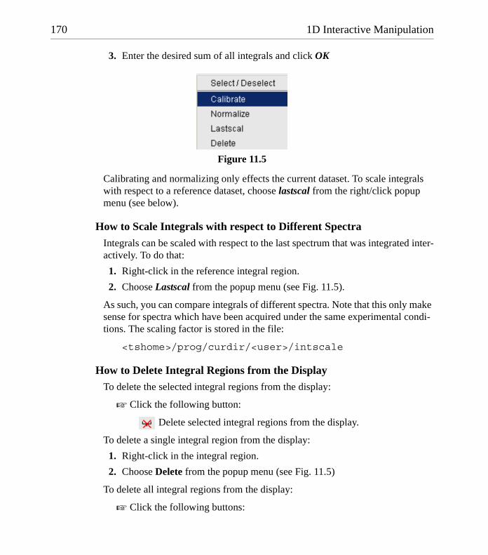
170 1D Interactive Manipulation
DONE
INDEX
INDEX
3. Enter the desired sum of all integrals and click OK
Calibrating and normalizing only effects the current dataset. To scale integrals with respect to a reference dataset, choose lastscal from the right/click popup menu (see below).
How to Scale Integrals with respect to Different Spectra
Integrals can be scaled with respect to the last spectrum that was integrated inter-actively. To do that:
1. Right-click in the reference integral region.
2. Choose Lastscal from the popup menu (see Fig. 11.5).
As such, you can compare integrals of different spectra. Note that this only make sense for spectra which have been acquired under the same experimental condi-tions. The scaling factor is stored in the file:
<tshome>/prog/curdir/<user>/intscale
How to Delete Integral Regions from the DisplayTo delete the selected integral regions from the display:
! Click the following button:
Delete selected integral regions from the display.
To delete a single integral region from the display:
1. Right-click in the integral region.
2. Choose Delete from the popup menu (see Fig. 11.5)
To delete all integral regions from the display:
! Click the following buttons:
Figure 11.5
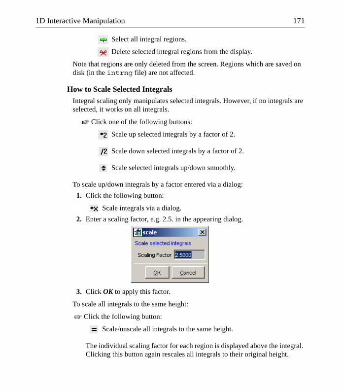
1D Interactive Manipulation 171
DONE
INDEX
INDEX
Select all integral regions.
Delete selected integral regions from the display.
Note that regions are only deleted from the screen. Regions which are saved on disk (in the intrng file) are not affected.
How to Scale Selected IntegralsIntegral scaling only manipulates selected integrals. However, if no integrals are selected, it works on all integrals.
! Click one of the following buttons:
Scale up selected integrals by a factor of 2.
Scale down selected integrals by a factor of 2.
Scale selected integrals up/down smoothly.
To scale up/down integrals by a factor entered via a dialog:
1. Click the following button:
Scale integrals via a dialog.
2. Enter a scaling factor, e.g. 2.5. in the appearing dialog.
3. Click OK to apply this factor.
To scale all integrals to the same height:
! Click the following button:
Scale/unscale all integrals to the same height.
The individual scaling factor for each region is displayed above the integral. Clicking this button again rescales all integrals to their original height.

172 1D Interactive Manipulation
DONE
INDEX
INDEX
How to Move the Integral Trails Up/Down
To move the integrals (selected and unselected) up or down:
! Click one of the following buttons:
The left edge of the lowest integral is put just above the baseline.
The right edge of the highest integral is put at 3/4 of the window height.
Shift all integral trails up/down smoothly.
How to Cut Integral Regions1. Click the following button (button turns green):
Cut integral region.
2. Move the red cursor line into an integral region to the position where it must be cut and click the left mouse button.
3. Do step 2 for each integral region that must be cut.
4. Click the (green) button to leave the cut integral mode (button turns grey).
How to Save Integral Regions1. Click the following button:
Save integral regions.
The following popup menu will appear:
2. Choose one of the following entries:
• Save regions to ’intrng’Save the currently displayed integral regions including the slope and bias correction values.
es
Figure 11.6
1D Interactive Manipulation 173
DONE
INDEX
INDEX
• Save Regions to ’reg’Save the integral regions to the file reg.
• Save & show listSave the currently displayed integral regions including the slope and bias correction values and show the integrals on the screen.
How to Undo the Last Region Operation
! Click the following button:
Undo the last region operation.
How to Return from the Integration Mode with/without SaveTo return and save the integrals to the current dataset:
! Click the following button:
Save integrals and return [.sret].
As such, you will:
• save the integral regions and corresponding slope and bias corrections to the file intrng.
• save the integral regions, slope and bias corrections and integral val-ues to the file integrals.txt. This file is displayed when you click the Integrals Tab.
• leave the integration mode.
To return without save:
! Click the following button:
Return, discarding any changes [.ret].
11.3 1D Interactive Calibration
A 1D spectrum can be calibrated (referenced), automatically, with the command sref or, interactively, as described below.
How to Switch to Calibration Mode
! Click the indicated button in the upper toolbar

174 1D Interactive Manipulation
DONE
INDEX
INDEX
or enter .cal on the command line. The Tab bar of the active data window will be replaced by a toolbar.
The yellow button indicates that the data window is in calibration mode.
How to Calibrate a Spectrum InteractivelyIn calibration mode:
1. Position the red cursor line at the reference peak.
2. Left-click at that position.
Figure 11.7 Data window in calibration mode
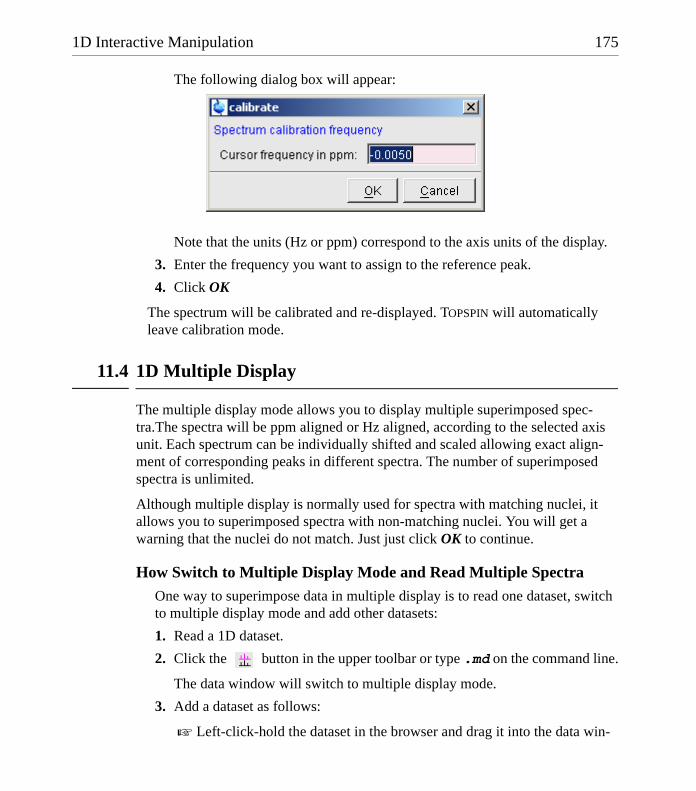
1D Interactive Manipulation 175
DONE
INDEX
INDEX
The following dialog box will appear:
Note that the units (Hz or ppm) correspond to the axis units of the display.
3. Enter the frequency you want to assign to the reference peak.
4. Click OK
The spectrum will be calibrated and re-displayed. TOPSPIN will automatically leave calibration mode.
11.4 1D Multiple Display
The multiple display mode allows you to display multiple superimposed spec-tra.The spectra will be ppm aligned or Hz aligned, according to the selected axis unit. Each spectrum can be individually shifted and scaled allowing exact align-ment of corresponding peaks in different spectra. The number of superimposed spectra is unlimited.
Although multiple display is normally used for spectra with matching nuclei, it allows you to superimposed spectra with non-matching nuclei. You will get a warning that the nuclei do not match. Just just click OK to continue.
How Switch to Multiple Display Mode and Read Multiple Spectra
One way to superimpose data in multiple display is to read one dataset, switch to multiple display mode and add other datasets:
1. Read a 1D dataset.
2. Click the button in the upper toolbar or type .md on the command line.
The data window will switch to multiple display mode.
3. Add a dataset as follows:
! Left-click-hold the dataset in the browser and drag it into the data win-

176 1D Interactive Manipulation
DONE
INDEX
INDEX
dow.
or
! Right-click the dataset in the browser and choose Display from the popup menu.
or
! Enter re and specify the additional dataset in the appearing dialog box.
Another way to superimpose data in multiple display is to read multiple datasets simultaneously:
1. In the browser or portfolio:
! Hold down the Ctrl key and click multiple datasets to select them.
or
! Hold down the Shift key and click two datasets to select these two and all datasets in between.
2. Right-click any of the selected data:
! Choose Display from the popup menu.This will show the data in the active data window if that is in multiple dis-play mode or, otherwise, show the data in a new window.
or
! Choose Display in new window from the popup menu.This will show the data in a new window.
In multiple display mode, the Tab bar of the active data window is replaced by a toolbar. Fig. 11.8 shows three comparable 1D spectra and the sum of all three.

1D Interactive Manipulation 177
DONE
INDEX
INDEX
The yellow button indicates that the data window is in multiple display mode.
Some buttons will turn green when they are clicked. As long as a button is green, it is active.
Furthermore, the browser/portfolio is split in two parts as shown in Fig. 11.9.
Figure 11.8 Data window in multiple display mode
Figure 11.9
178 1D Interactive Manipulation
DONE
INDEX
INDEX
The additional lower part shows:
• which datasets are displayed in the active data window.
• which datasets are selected (these are highlighted).
How to Select/Deselect DatasetsTo select a dataset:
! Click in the corresponding area in the data window.
or Click the small square at the upper right of the spectrum.
or Click the corresponding entry in the lower part of the browser/portfolio.
In the lower part of the browser/portfolio, you can:
! Click one dataset to select it.
or Hold down the Ctrl key and click multiple datasets to select them.
or Hold down the Shift key and click two datasets to select these two and all datasets in between.
When you select a dataset, the corresponding small square is filled (see Fig. 11.8) and its entry in the lower part of the browser is highlighted (see Fig. 11.9).
Note that:
• no spectrum selected = all spectra selected
• scale/shift buttons of the data window toolbar only work on selected spectra
To deselect a dataset:
! Select a different dataset.
To deselect all datasets:
! Click the following button:
Deselect all datasets.
How to Remove a Dataset from Multiple Display1. Select the dataset(s) you want to remove.
2. Click the following button:
1D Interactive Manipulation 179
DONE
INDEX
INDEX
Remove selected data from the screen.
Note that the data on disk are not affected. Furthermore, the first spectrum cannot be removed from the screen.
How to Display the Sum or Difference Spectra
! Click one of the following button (button turns green):
Show the difference between the first and the sum of the other datasets.
Show the sum of all datasets in the multiple display window.
How to Save the Sum or Difference Spectra1. Click the following button:
Save the displayed sum or difference spectrum.
2. In the appearing dialog box, specify the destination procno.
How to Display the Next/Previous Name/Expno
To compare a series of spectra you can interactively increment or decrement the dataset name or expno. A dataset name is incremented according to the ICON-NMR naming convention of increasing extensions, e.g. name.001, name.002 etc.
! Click one of the following button (button turns green):
Show the previous name/expno.
Show the previous name/expno.
Set the increment options. Clicking this button will open the following dialog:

180 1D Interactive Manipulation
DONE
INDEX
INDEX
Here you can choose to increment the expno or name, set the expno incre-
ment and switch individual scaling on/off.
How to Toggle between Superimposed and Stacked Display
! Click the following button:
Toggle between superimposed and stacked display.
How to Shift and Scale Individual Spectra
To compare the intensity and chemical shift of corresponding peaks, you can shift and scale individual spectra. To do this:
1. Display the spectra in multiple display mode as described above.
2. Expand the spectra to display the desired region or peak.
3. Select one of the spectra (e.g. by clicking it in the lower part of the browser).
4. Click-hold the button and move the mouse to align the intensities.
5. Click-hold the button and move the mouse to align the peak positions.
The alignment can be facilitated by showing the difference spectrum ( button) and minimize that. Clicking the button resets individual scaling and shifting.
The performed scaling and shifting are displayed in the data window (see Fig. 11.10 and 11.11).

1D Interactive Manipulation 181
DONE
INDEX
INDEX
How to Switch on/off the Display of Datapaths and Scaling Factors
! Click the following button:
Switch on/off display of datapaths and scaling factors.
Figure 11.10
Figure 11.11

182 1D Interactive Manipulation
DONE
INDEX
INDEX
How to Return from Multiple Display mode
! Click the following button:
Return from multiple display mode [.ret].
How to Set the Colors of the 1st, 2nd, .. DatasetThe colors of the different datasets in the multiple display mode can be set in the User preferences dialog box. To set, for example, the color of the second spec-trum:
! Click Options " Preferences and click the Change button for the item Color of 2nd 1D spectrum.
11.5 1D Interactive Baseline Correction
Baseline correction can be performed with commands like abs or absd or, inter-actively, as described below.
How to Switch to Baseline Correction Mode
! Click the indicated button in the upper toolbar:
or enter .basl on the command line.
The Tab bar of the active data window will be replaced by a toolbar (see Fig. 11.12).

1D Interactive Manipulation 183
DONE
INDEX
INDEX
The yellow button indicates that the data window is in baseline correc-tion mode.
Some buttons will turn green when they are clicked. As long as a button is green, it is active.
How to Perform Polynomial Baseline Correction1. Click the following button (button turns green):
Perform polynomial baseline correction.
In the data window, a red horizontal line will appear as well as the equation that describes the polynomial function:
2. Click-hold button A and move the mouse until the red line coincides with the first point of the spectrum.
3. Repeat step 2 with the buttons B, C, D and E until the red line coincides with the entire baseline of the spectrum.
How to Perform Sine Baseline Correction1. Click the following button (button turns green):
Figure 11.12 Data window in baseline correction mode

184 1D Interactive Manipulation
DONE
INDEX
INDEX
Perform sine baseline correction.
A red horizontal line will appear as well as the equation describing the sine function:
2. Click-hold button A and move the mouse until the red line coincides with the first point of the spectrum.
3. Repeat step 2 with the buttons B, C and D until the red line coincides with the entire baseline of the spectrum.
How to Perform Exponential Baseline Correction1. Click the following button (button turns green):
Perform exponential baseline correction.
A red horizontal line will appear as well as the equation describing the ex-ponential function:
2. Click-hold button A and move the mouse until the red line coincides with the first point of the spectrum.
3. Repeat step 2 with the buttons B and C until the red line coincides with the entire baseline of the spectrum.
How to Preview the Baseline Corrected SpectrumBefore actually performing the baseline correction, you can preview the result by displaying the difference between the uncorrected spectrum and the red correction line.
To do that:
1. Click the following button (button turns green):
Preview corrected spectrum (show difference).
The corrected spectrum will be displayed in red.
2. If the baseline is correct, click the button to save the correction. If fur-ther correction is needed, click the button to show the original spectrum and the red correction line.
1D Interactive Manipulation 185
DONE
INDEX
INDEX
How to Reset the Baseline Correction Line1. Click the following button:
Reset the red correction line to zero.
If the difference spectrum is displayed (the button is active), clicking the reset button will restore the original spectrum.
How to Change the Mouse Sensitivity ! Click one of the following buttons:
Increase (double) the Mouse Sensitivity [.inc].
Decrease (halve) the Mouse Sensitivity [.dec].
Reset the Mouse Sensitivity.
How to Save the Baseline Correction and/or ReturnTo return while saving the baseline correction:
! Click the following button:
Save baseline correction and Return [.sret]
This will perform the following tasks:
• Execute the baseline correction [bcm].
• Save the baseline correction values A, B, C, D and E.
• Leave the baseline correction mode.
To return while discarding any changes:
Click the following button:
Return, Discarding any changes [.ret].
How to Perform Cubic Spline Baseline correction
! Click the following button:
Define points for cubic spline baseline correction.
The toolbar of the data window will change as shown in Fig. 11.13.
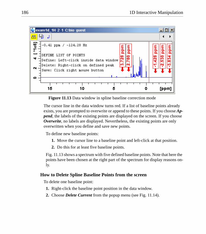
186 1D Interactive Manipulation
DONE
INDEX
INDEX
The cursor line in the data window turns red. If a list of baseline points already exists, you are prompted to overwrite or append to these points. If you choose Ap-pend, the labels of the existing points are displayed on the screen. If you choose Overwrite, no labels are displayed. Nevertheless, the existing points are only overwritten when you define and save new points.
To define new baseline points:
1. Move the cursor line to a baseline point and left-click at that position.
2. Do this for at least five baseline points.
Fig. 11.13 shows a spectrum with five defined baseline points. Note that here the points have been chosen at the right part of the spectrum for display reasons on-ly.
How to Delete Spline Baseline Points from the screen
To delete one baseline point:
1. Right-click the baseline point position in the data window.
2. Choose Delete Current from the popup menu (see Fig. 11.14).
Figure 11.13 Data window in spline baseline correction mode

1D Interactive Manipulation 187
DONE
INDEX
INDEX
To delete all baseline points:
1. Right-click any position in the data window.
2. Choose Delete All from the popup menu (see Fig. 11.14).
How to Return from Cubic Spline Baseline mode with/without Save
To return while saving the baseline points:
! Click the following button:
Save baseline points and Return [.retsab].
To return while discarding any changes:
! Click the following button:
Return, Discarding any changes [.ret].
Alternatively, you can right-click in the data window and choose Save & Quit or Quit, respectively.
11.6 1D Interactive Peak Picking
Peak picking can be performed, automatically, with the commands pps or, interac-tively, in the peak picking mode.
Figure 11.14

188 1D Interactive Manipulation
DONE
INDEX
INDEX
How to Switch to Peak Picking Mode
! Click the indicated button in the upper toolbar:
or enter .pp on the command line.
The Tab bar of the active data window will be replaced by a toolbar (see Fig. 11.15).
The yellow button indicates that you are in peak picking mode.
Some buttons will turn green when they are clicked. As long as a button is green, it is active.
Note that the button is automatically activated, i.e. you are in Define peak picking range mode
How to Define New Peak Picking Ranges1. Put the cursor at the upper-left corner of a peak picking range.
Figure 11.15 Data window in peak picking mode

1D Interactive Manipulation 189
DONE
INDEX
INDEX
2. Left-click-hold and drag the mouse to the lower-right corner of the range.
The peak picking range will be marked green. The minimum and maximum intensity are set and the peaks in the range are picked and displayed.
3. Repeat step 1 and 2 for each peak picking range to be defined.
4. Click the green button to leave the "Define peak picking range" mode.
Note that the parameters MI and MAXI are set to the lowest minimum and the highest maximum intensity, respectively, of all ranges.
How to Change Peak Picking Ranges1. Click the following button (button turns green):
Change peak picking ranges.
2. Put the cursor on one of the edges of the peak picking range.
The cursor turns into a double-headed arrow.
3. Left-click-hold and drag the peak range edge to its new position.
4. Optionally: repeat step 2 and 3 for the other edge and for other peak ranges.
5. Click the green button to leave the "Change peak picking range" mode.
How to Pick Peaks in Peak Picking Ranges only
Peaks in a peak range are automatically picked when the range is defined.If peaks have been deleted from a rang, they can be picked again as follows:
1. Right-click in the data field.
2. Choose Pick Peaks On Ranges from the popup menu.
Alternatively, you can enter ppl on the command line. This command can be en-tered in Interactive peak picking mode or in the normal display mode.
How to Delete all Peak Picking Ranges
! Click the button in the data window toolbar.
or
! Right-click in the data field and click Delete All Ranges in the popup menu.
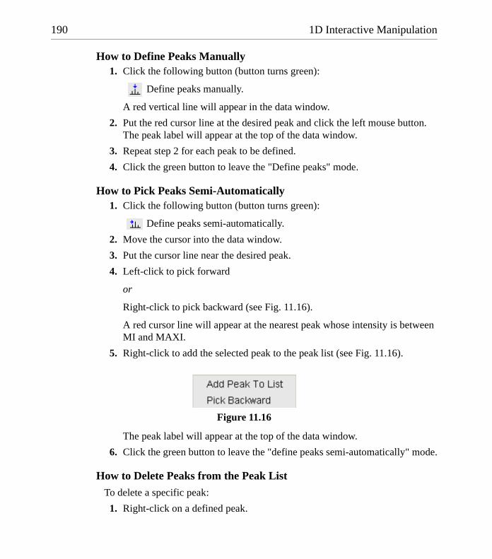
190 1D Interactive Manipulation
DONE
INDEX
INDEX
How to Define Peaks Manually1. Click the following button (button turns green):
Define peaks manually.
A red vertical line will appear in the data window.
2. Put the red cursor line at the desired peak and click the left mouse button.The peak label will appear at the top of the data window.
3. Repeat step 2 for each peak to be defined.
4. Click the green button to leave the "Define peaks" mode.
How to Pick Peaks Semi-Automatically1. Click the following button (button turns green):
Define peaks semi-automatically.
2. Move the cursor into the data window.
3. Put the cursor line near the desired peak.
4. Left-click to pick forward
or
Right-click to pick backward (see Fig. 11.16).
A red cursor line will appear at the nearest peak whose intensity is between MI and MAXI.
5. Right-click to add the selected peak to the peak list (see Fig. 11.16).
The peak label will appear at the top of the data window.
6. Click the green button to leave the "define peaks semi-automatically" mode.
How to Delete Peaks from the Peak List
To delete a specific peak:
1. Right-click on a defined peak.
Figure 11.16

1D Interactive Manipulation 191
DONE
INDEX
INDEX
2. Choose Delete peak under cursor from the popup menu (see Fig. 11.17). 99
To delete all peaks:
! Click the button in the data window toolbar.
or
! Right-click in the data field and click Delete All Peaks in the popup menu.
How to Return from Peak Picking Mode with/without SaveTo return while saving the peak list and peak ranges:
! Click the following button:
Save the Peak Region and Peak List and Return [.sret].
This will:
• Save the peak list to the file peak.txt and the peak ranges to the file peakrng.
• Leave the peak picking mode.
To return while discarding any changes:
! Click the following button:
Return, discarding any changes [.ret].
Figure 11.17


Chapter 12
2D Interactive Manipulation
The upper toolbar of the 2D menu offers various buttons for interactive manipula-tion. If you click such a button, the active data window will switch to the corre-sponding mode. An interactive manipulation mode is data window specific, i.e. it only applies to the active window.
12.1 2D Interactive Phase Correction
2D spectra can be phase corrected interactively in both the F2 and F1 direction by selecting certain rows and/or columns and phase correct them.
12.1.1 2D Interactive Phase Correction Procedure
How to Switch to 2D Interactive Phase CorrectionClick the corresponding button in the upper toolbar as indicated below:
or enter .ph on the command line.
The Tab bar of the active data window will be replaced by a toolbar. Fig. 12.1
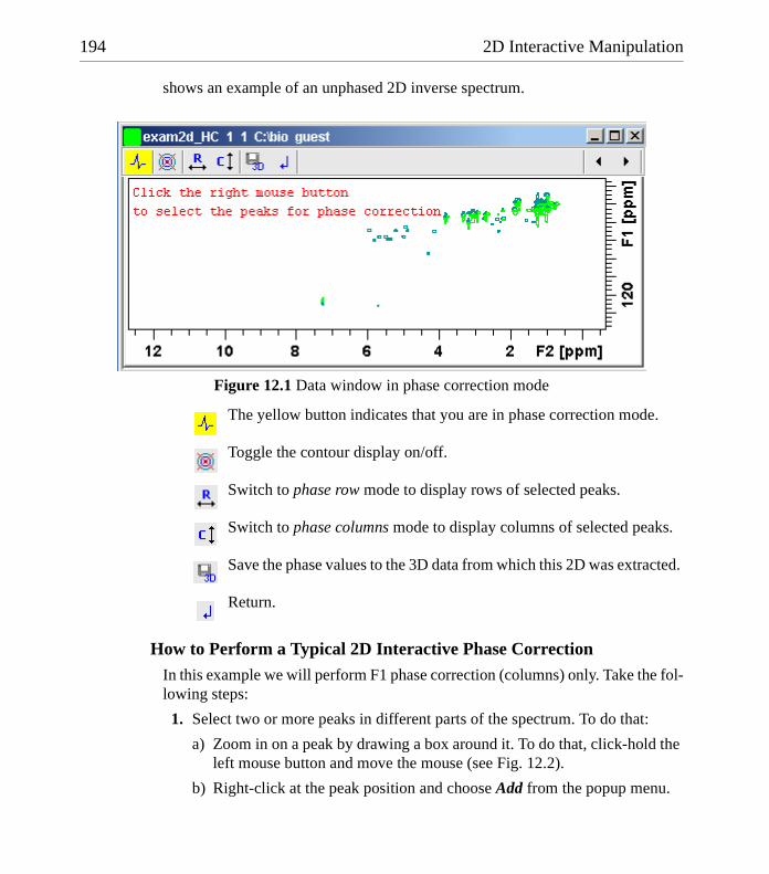
194 2D Interactive Manipulation
DONE
INDEX
INDEX
shows an example of an unphased 2D inverse spectrum.
The yellow button indicates that you are in phase correction mode.
Toggle the contour display on/off.
Switch to phase row mode to display rows of selected peaks.
Switch to phase columns mode to display columns of selected peaks.
Save the phase values to the 3D data from which this 2D was extracted.
Return.
How to Perform a Typical 2D Interactive Phase CorrectionIn this example we will perform F1 phase correction (columns) only. Take the fol-lowing steps:
1. Select two or more peaks in different parts of the spectrum. To do that:
a) Zoom in on a peak by drawing a box around it. To do that, click-hold the left mouse button and move the mouse (see Fig. 12.2).
b) Right-click at the peak position and choose Add from the popup menu.
Figure 12.1 Data window in phase correction mode
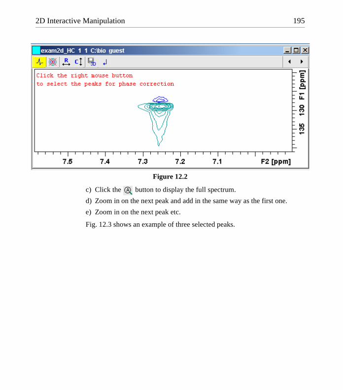
2D Interactive Manipulation 195
DONE
INDEX
INDEX
c) Click the button to display the full spectrum.
d) Zoom in on the next peak and add in the same way as the first one.
e) Zoom in on the next peak etc.
Fig. 12.3 shows an example of three selected peaks.
Figure 12.2
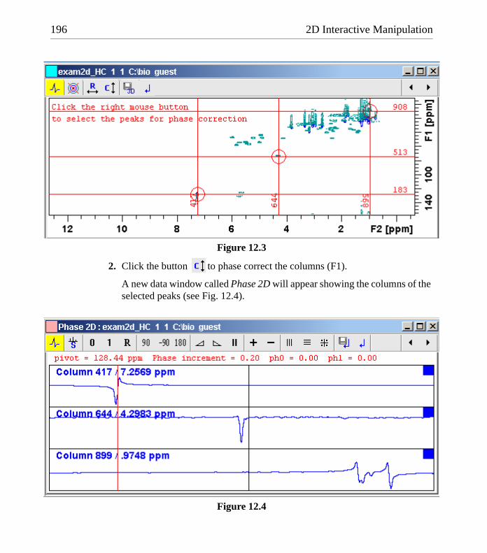
196 2D Interactive Manipulation
DONE
INDEX
INDEX
2. Click the button to phase correct the columns (F1).
A new data window called Phase 2D will appear showing the columns of the selected peaks (see Fig. 12.4).
Figure 12.3
Figure 12.4
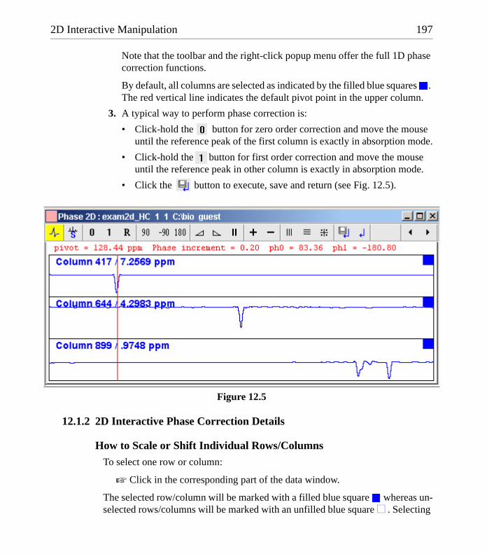
2D Interactive Manipulation 197
DONE
INDEX
INDEX
Note that the toolbar and the right-click popup menu offer the full 1D phase correction functions.
By default, all columns are selected as indicated by the filled blue squares . The red vertical line indicates the default pivot point in the upper column.
3. A typical way to perform phase correction is:
• Click-hold the button for zero order correction and move the mouse until the reference peak of the first column is exactly in absorption mode.
• Click-hold the button for first order correction and move the mouse until the reference peak in other column is exactly in absorption mode.
• Click the button to execute, save and return (see Fig. 12.5).
12.1.2 2D Interactive Phase Correction Details
How to Scale or Shift Individual Rows/ColumnsTo select one row or column:
! Click in the corresponding part of the data window.
The selected row/column will be marked with a filled blue square whereas un-selected rows/columns will be marked with an unfilled blue square . Selecting
Figure 12.5
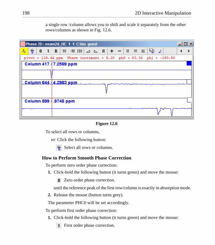
198 2D Interactive Manipulation
DONE
INDEX
INDEX
a single row /column allows you to shift and scale it separately from the other rows/columns as shown in Fig. 12.6.
To select all rows or columns,
! Click the following button:
Select all rows or columns.
How to Perform Smooth Phase Correction
To perform zero order phase correction:
1. Click-hold the following button (it turns green) and move the mouse:
Zero order phase correction.
until the reference peak of the first row/column is exactly in absorption mode.
2. Release the mouse (button turns grey).
The parameter PHC0 will be set accordingly.
To perform first order phase correction:
1. Click-hold the following button (it turns green) and move the mouse:
First order phase correction.
Figure 12.6

2D Interactive Manipulation 199
DONE
INDEX
INDEX
until the reference peak of the second and further rows/columns is exactly in absorption mode.
2. Release the mouse (button turns grey).
The parameter PHC1 will be set accordingly.
How to Perform 90, -90 or 180° Zero Order Phase CorrectionClick one of the following buttons:
90° zero order phase correction.
-90° zero order phase correction.
180° zero order phase correction.
How to Reset the Phase to the Original ValuesClick the following button:
Reset zero and first order phase.
How to Change the Mouse Sensitivity
Click one of the following buttons:
Increase (double) the mouse sensitivity [.inc].
Decrease (halve) the mouse sensitivity [.dec].
Reset the mouse sensitivity to 1.0.
How to Show the Next/Previous Row or Column
To show the next row/column, click the following button:
Show next row/column.
Note that only the selected row/column is increased. If all rows/columns are se-lected, only the first one is increased.
To show the previous row/column, click the following button:
Show previous row/column.
200 2D Interactive Manipulation
DONE
INDEX
INDEX
Note that only the selected row/column is decreased. If all rows/columns are se-lected, only the first one is decreased.
How to Arrange Rows or ColumnsClick one of the following buttons:
Arrange rows/columns horizontally.
Arrange rows/columns vertically (see Fig. 12.6).
Arrange rows/columns vertically in a split window.
How to Return from Multi-1D Phase to 2D Phase Display Click the following button:
to save, execute and return.
This will perform the following tasks:
• Execute phase correction.
• Save the current phase correction values.
• Leave the multi-1D phase mode.
Click the following button:
to return to the 2D phase display without save.
How to Return from 2D Phase Mode
Click the following button:
Return.
12.2 2D Multiple Display and Row/Column Handling
2D multiple display shows a 2D spectrum with an arbitrary number of 1D and/or 2D spectra superimposed.
Spectra are ppm aligned or Hz aligned, according to the selected axis unit.
A superimposed 1D spectrum is automatically displayed in the direction of the matching nucleus (for a hetero-nuclear 2D) or in the F2 direction (for a homo-
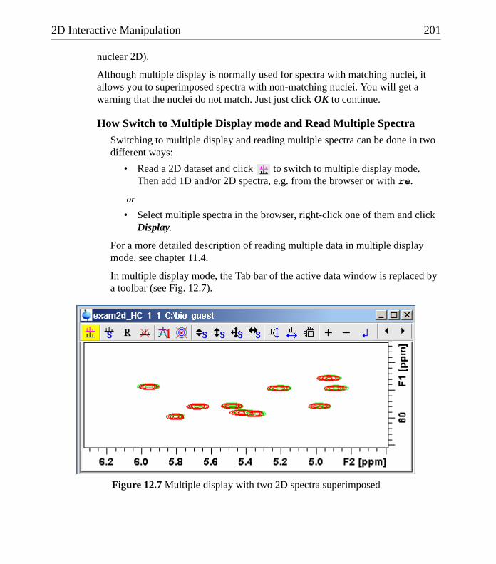
2D Interactive Manipulation 201
DONE
INDEX
INDEX
nuclear 2D).
Although multiple display is normally used for spectra with matching nuclei, it allows you to superimposed spectra with non-matching nuclei. You will get a warning that the nuclei do not match. Just just click OK to continue.
How Switch to Multiple Display mode and Read Multiple SpectraSwitching to multiple display and reading multiple spectra can be done in two different ways:
• Read a 2D dataset and click to switch to multiple display mode. Then add 1D and/or 2D spectra, e.g. from the browser or with re.
or
• Select multiple spectra in the browser, right-click one of them and click Display.
For a more detailed description of reading multiple data in multiple display mode, see chapter 11.4.
In multiple display mode, the Tab bar of the active data window is replaced by a toolbar (see Fig. 12.7).
Figure 12.7 Multiple display with two 2D spectra superimposed

202 2D Interactive Manipulation
DONE
INDEX
INDEX
The yellow button indicates that the data window is in multiple display mode.
Some buttons will turn green when they are clicked. As long as a button is green, it is active.
The browser/portfolio in multiple display is split in two parts (see Fig. 12.9).The additional lower part shows:
• which datasets are displayed in the active data window
• which datasets are selected (they are highlighted)
Figure 12.8 Multiple display with a 1D spectrum superimposed on a 2D spectrum
Figure 12.9

2D Interactive Manipulation 203
DONE
INDEX
INDEX
How to Align Multiple 2D Spectra
2D spectra in multiple display can be individually shifted. To do that:
1. Select one of the spectra in the lower part of the browser.
2. Click-hold the button and move the mouse.
Fig. 12.10 shows a region of two comparable 1H/13C inverse 2D datasets which are shifted relative to each other.
Clicking the button resets individual scaling and shifting.
How to Scan Rows/Columns
Click the following button (it turns green) and move the mouse in the data field:
to scan rows in the 2D spectrum.
Click the following button (it turns green) and move the mouse in the data field:
to scan columns in the 2D spectrum.
To scale up the displayed row/column:
! Click the left mouse button or turn the mouse wheel up.
To scale down the displayed row/column:
Figure 12.10
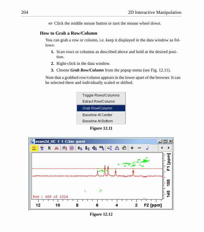
204 2D Interactive Manipulation
DONE
INDEX
INDEX
! Click the middle mouse button or turn the mouse wheel down.
How to Grab a Row/ColumnYou can grab a row or column, i.e. keep it displayed in the data window as fol-lows:
1. Scan rows or columns as described above and hold at the desired posi-tion.
2. Right-click in the data window.
3. Choose Grab Row/Column from the popup menu (see Fig. 12.11).
Note that a grabbed row/column appears in the lower apart of the browser. It can be selected there and individually scaled or shifted.
Figure 12.11
Figure 12.12
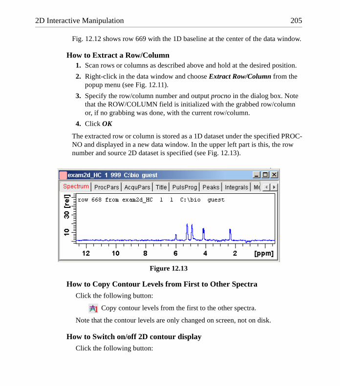
2D Interactive Manipulation 205
DONE
INDEX
INDEX
Fig. 12.12 shows row 669 with the 1D baseline at the center of the data window.
How to Extract a Row/Column1. Scan rows or columns as described above and hold at the desired position.
2. Right-click in the data window and choose Extract Row/Column from the popup menu (see Fig. 12.11).
3. Specify the row/column number and output procno in the dialog box. Note that the ROW/COLUMN field is initialized with the grabbed row/column or, if no grabbing was done, with the current row/column.
4. Click OK
The extracted row or column is stored as a 1D dataset under the specified PROC-NO and displayed in a new data window. In the upper left part is this, the row number and source 2D dataset is specified (see Fig. 12.13).
How to Copy Contour Levels from First to Other Spectra
Click the following button:
Copy contour levels from the first to the other spectra.
Note that the contour levels are only changed on screen, not on disk.
How to Switch on/off 2D contour display
Click the following button:
Figure 12.13

206 2D Interactive Manipulation
DONE
INDEX
INDEX
Switch on/off 2D contour display.
How to Position the Baseline of the Row/ColumnTo put the baseline at the center of the data window:
1. Right-click in the data window.
2. Choose in Baseline At Center from the popup menu (see Fig. 12.11).
To put the baseline at the bottom of the data window:
1. Right-click in the data window.
2. Choose in Baseline At Bottom from the popup menu (see Fig. 12.11).
This works both in the scan submode or on a grabbed row/column.
12.3 2D Interactive Calibration
A 2D spectrum can be calibrated, automatically with the command sref or, inter-actively as described below.
How to Switch to 2D Calibration mode
! Click the corresponding button in the upper toolbar:.
The Tab bar of the active data window will be replaced by a toolbar (see Fig. 12.14).
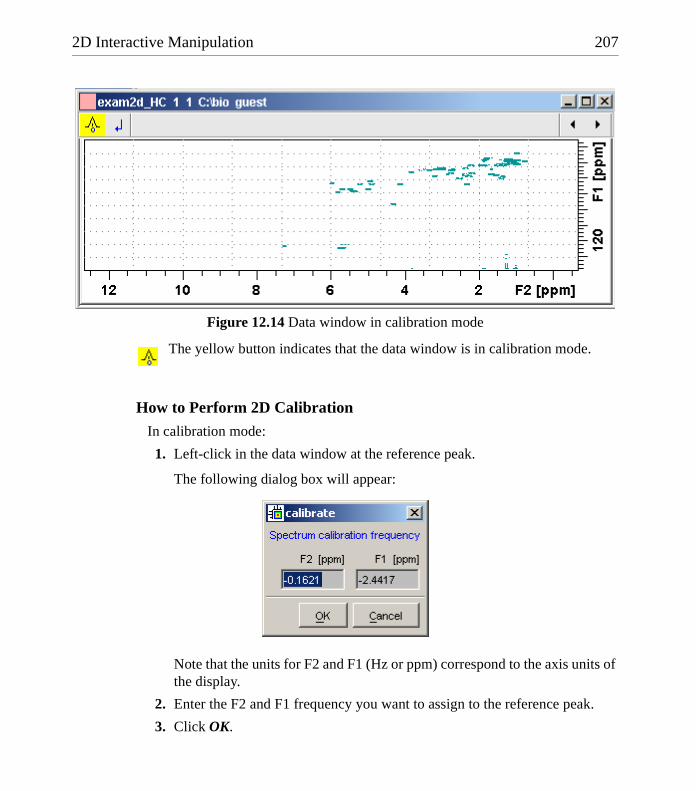
2D Interactive Manipulation 207
DONE
INDEX
INDEX
The yellow button indicates that the data window is in calibration mode.
How to Perform 2D Calibration
In calibration mode:
1. Left-click in the data window at the reference peak.
The following dialog box will appear:
Note that the units for F2 and F1 (Hz or ppm) correspond to the axis units of the display.
2. Enter the F2 and F1 frequency you want to assign to the reference peak.
3. Click OK.
Figure 12.14 Data window in calibration mode
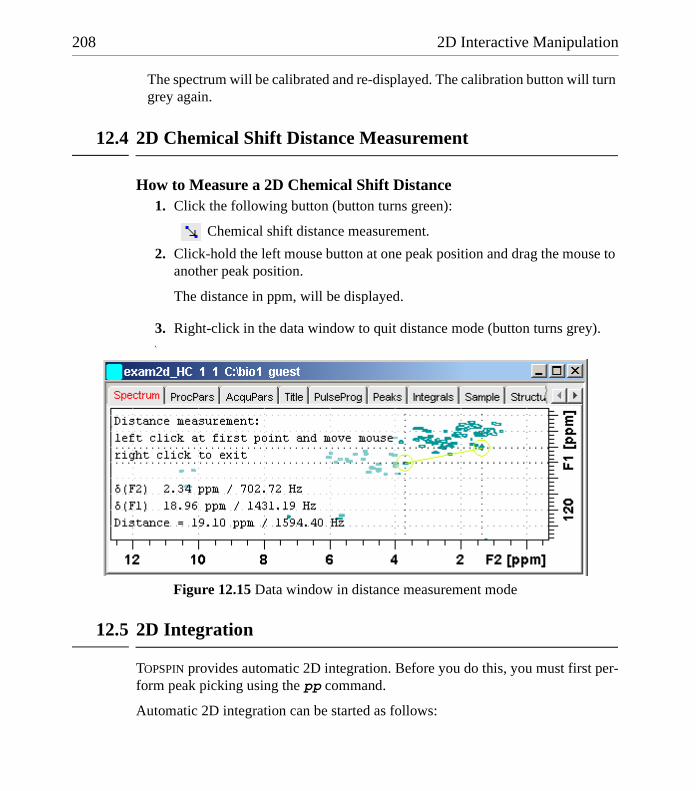
208 2D Interactive Manipulation
DONE
INDEX
INDEX
The spectrum will be calibrated and re-displayed. The calibration button will turn grey again.
12.4 2D Chemical Shift Distance Measurement
How to Measure a 2D Chemical Shift Distance 1. Click the following button (button turns green):
Chemical shift distance measurement.
2. Click-hold the left mouse button at one peak position and drag the mouse to another peak position.
The distance in ppm, will be displayed.
3. Right-click in the data window to quit distance mode (button turns grey).4.
12.5 2D Integration
TOPSPIN provides automatic 2D integration. Before you do this, you must first per-form peak picking using the pp command.
Automatic 2D integration can be started as follows:
Figure 12.15 Data window in distance measurement mode
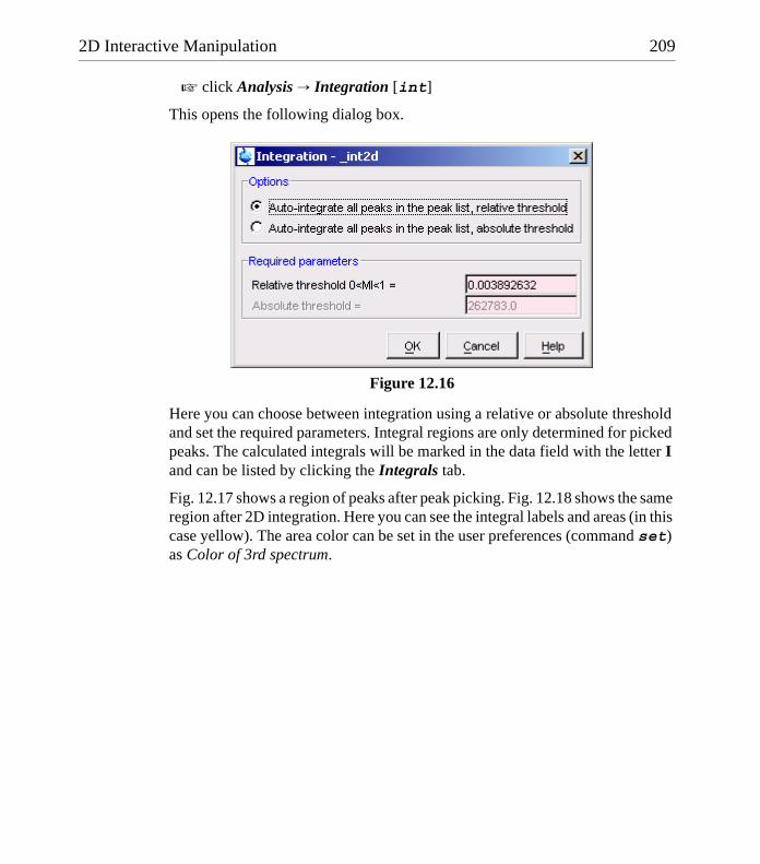
2D Interactive Manipulation 209
DONE
INDEX
INDEX
! click Analysis " Integration [int]
This opens the following dialog box.
Here you can choose between integration using a relative or absolute threshold and set the required parameters. Integral regions are only determined for picked peaks. The calculated integrals will be marked in the data field with the letter I and can be listed by clicking the Integrals tab.
Fig. 12.17 shows a region of peaks after peak picking. Fig. 12.18 shows the same region after 2D integration. Here you can see the integral labels and areas (in this case yellow). The area color can be set in the user preferences (command set) as Color of 3rd spectrum.
Figure 12.16
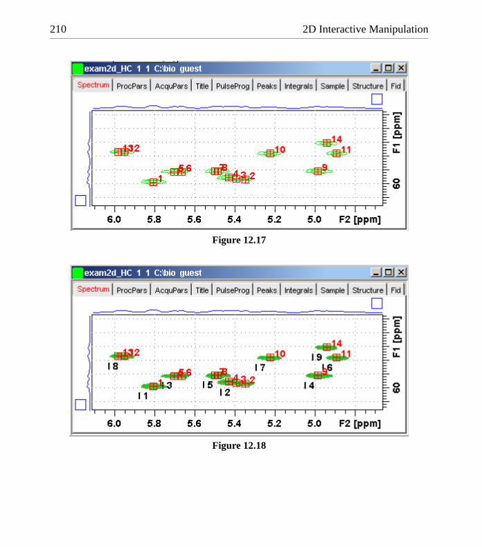
210 2D Interactive Manipulation
DONE
INDEX
INDEX
Figure 12.17
Figure 12.18
Chapter 13
Data Window Handling
13.1 Data Windows
The TOPSPIN window has a data area that may contain multiple data windows. The size of the data area depends on the overall size of the TOPSPIN window and on presence of the Browser and/or Processing Guide. Fig. 13.1 shows the TOPSPIN window with the Browser and three data windows.

212 Data Window Handling
DONE
INDEX
INDEX
Note that the three data windows show different data objects: 1D processing parameters, a 1D spectrum and a 2D spectrum.
How to Move a Data Window
! Click-hold the title bar and move the mouse.
How to Resize a Data Window1. Move the cursor to the window edge until it becomes a double-headed
arrow.
2. Left-click-hold that position and move the mouse.
Depending on the position of the double-headed arrow, you can change the win-dow height, width or both (see Fig. 13.2)
Figure 13.1
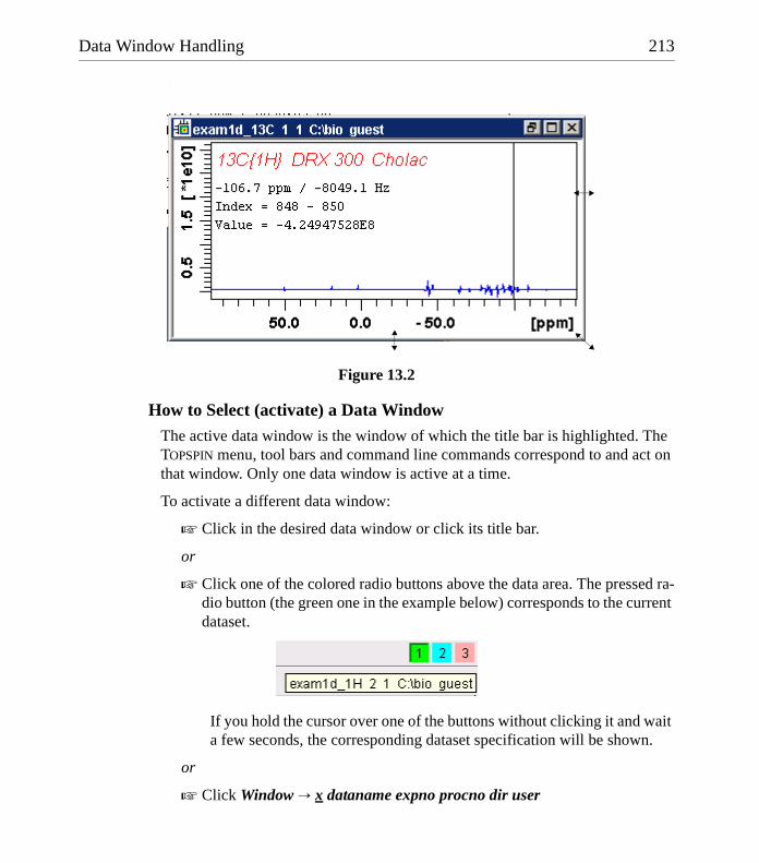
Data Window Handling 213
DONE
INDEX
INDEX
.
How to Select (activate) a Data Window
The active data window is the window of which the title bar is highlighted. The TOPSPIN menu, tool bars and command line commands correspond to and act on that window. Only one data window is active at a time.
To activate a different data window:
! Click in the desired data window or click its title bar.
or
! Click one of the colored radio buttons above the data area. The pressed ra-dio button (the green one in the example below) corresponds to the current dataset.
If you hold the cursor over one of the buttons without clicking it and wait a few seconds, the corresponding dataset specification will be shown.
or
! Click Window " x dataname expno procno dir user
Figure 13.2

214 Data Window Handling
DONE
INDEX
INDEX
where x is the number of the desired window and dataname, expno, proc-no, dir and user refer to the dataset displayed in that window.
or
! Hit the F6 key to activate the next window. Repeat that until the desired window is the active window.
How to Open a New empty Data Window! Click Window " New window [Alt+w-n]
The new data window will become the active window and will, by default, cover the entire data area, hiding possible existing data windows. To open a dataset in the new window, drag a dataset from the browser or from the Windows Explorer into the new window or click File " Open (see also chapter 4.3).
How to Arrange Data WindowsIf the data area contains multiple data windows, you can arrange them in various ways. All the arrange commands arrange the windows left to right and/or top to bottom in the order in which the windows have been active. The currently active data window will therefore be positioned at the top and/or left of the data area.
To arrange the data windows as a grid:
! Click Window " Arrange as a Grid
Depending on the number of windows, they will be arranged vertically and/or horizontally (see Fig. 13.3).

Data Window Handling 215
DONE
INDEX
INDEX
To arrange data windows in stack (see Fig. 13.4):
! Click Window " Arrange in Stack
Figure 13.3
Figure 13.4

216 Data Window Handling
DONE
INDEX
INDEX
To arrange data windows side by side (see Fig. 13.5):
! Click Window " Arrange Side-by-Side
To cascade data windows (see Fig. 13.6):
! Click Window " Cascade
Note that you can instruct TOPSPIN to open new data windows cascaded rather than maximized as well configure cascaded windows (command set " Window set-tings, see also chapter 4.3)
How to Iconify (minimize) a Data Window
! Click the button in the windows title bar
Figure 13.5
Figure 13.6
Data Window Handling 217
DONE
INDEX
INDEX
or
! Click Window " Iconify all to iconify all windows.
How to De-iconify a Data Window
! Click the button or double-click the title bar.
How to Maximize a Data Window
! Click the button or double-click the title bar.
The window will cover the entire data area. Note that a maximized window can-not be moved of resized but can be restored (in size and position), iconified or closed.
How to Restore the Size and Position of a Data Window
! Click the button or double-click the title bar.
Note that this is only possible if the title bar contains the button. This is only the case after the window has been maximized or iconified.
How to Close a Data WindowTo close the active data window:
! Click File " Close [Crtl-w]
or
! Click the button in the windows title bar.
To close any data window:
! Click the button in the data windows title bar
or
! Click the title bar and then click File " Close [Crtl-w].
To close all data windows:
! Click File " Closeall [closeall]

218 Data Window Handling
DONE
INDEX
INDEX
How to Iconify all Data Windows
! Click Window " Iconify all
How to Maximize all Data Windows! Click Window " Maximize all
The active window will be displayed on top, all other windows are hidden.
How to Activate the Next Data Window
! Click Window " Next window [F6].
The windows title bar will become highlighted.
13.2 Window Layouts
A data window layout defines the position, geometry and window type of one or more TOPSPIN windows. The following windows types are available:
• data windows
• lock display window
• acquisition display window
• BSMS display window
• temperature unit window
How to Save the Current Window Layout1. Click Window " Save layout
2. In the appearing dialog box:Specify the layout File name (extension .prop) and click Save Layout
How to Read a Window Layout 1. Click Window " Read layout
2. In the appearing dialog box:Specify or click the layout File name and click Read Layout
Windows are arranged according to the following rules:
Data Window Handling 219
DONE
INDEX
INDEX
• Each currently displayed window type gets the position and geometry to the corresponding definition in the layout.
• If a window type is displayed but not defined in the layout, it keeps its current position and geometry.
• If a window type is defined in the layout but not displayed, the layout definition is ignored.
• Multiple data windows are, arbitrarily, assigned to the available data window definitions.
How to Swap Data WindowsWithin a certain layout, you can easily swap two TOPSPIN windows with the com-mand swin. If the data area contains exactly two windows, swin simple swaps their position and geometry. If it contains more than two data windows, swin opens a list from which you can select any window to be swapped with the cur-rently selected (active) window. Swapping windows can also be executed from the Window menu.


Chapter 14
Analysis
This chapter describes various TOPSPIN analysis methods including chemical shift measurement, signal to noise calculation, solids line shape analysis, T1/T2 relaxa-tion analysis and multiplet analysis.
14.1 1D Chemical Shift Distance Measurement
How to Measure a Chemical Shift Distance 1. Click the following button (button turns green):
Chemical shift distance measurement.
2. Left-click-hold at one peak position and drag the mouse to another peak position.
The distance in ppm, will be displayed.
3. Right-click in the data window or move the cursor out of the data window to leave distance measurement mode (button turns grey).
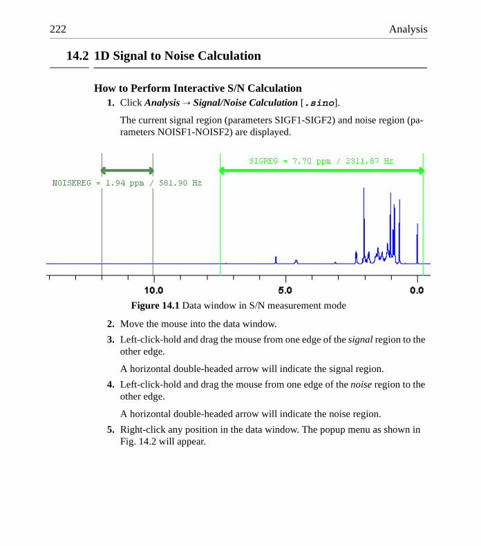
222 Analysis
DONE
INDEX
INDEX
14.2 1D Signal to Noise Calculation
How to Perform Interactive S/N Calculation1. Click Analysis " Signal/Noise Calculation [.sino].
The current signal region (parameters SIGF1-SIGF2) and noise region (pa-rameters NOISF1-NOISF2) are displayed.
2. Move the mouse into the data window.
3. Left-click-hold and drag the mouse from one edge of the signal region to the other edge.
A horizontal double-headed arrow will indicate the signal region.
4. Left-click-hold and drag the mouse from one edge of the noise region to the other edge.
A horizontal double-headed arrow will indicate the noise region.
5. Right-click any position in the data window. The popup menu as shown in Fig. 14.2 will appear.
Figure 14.1 Data window in S/N measurement mode
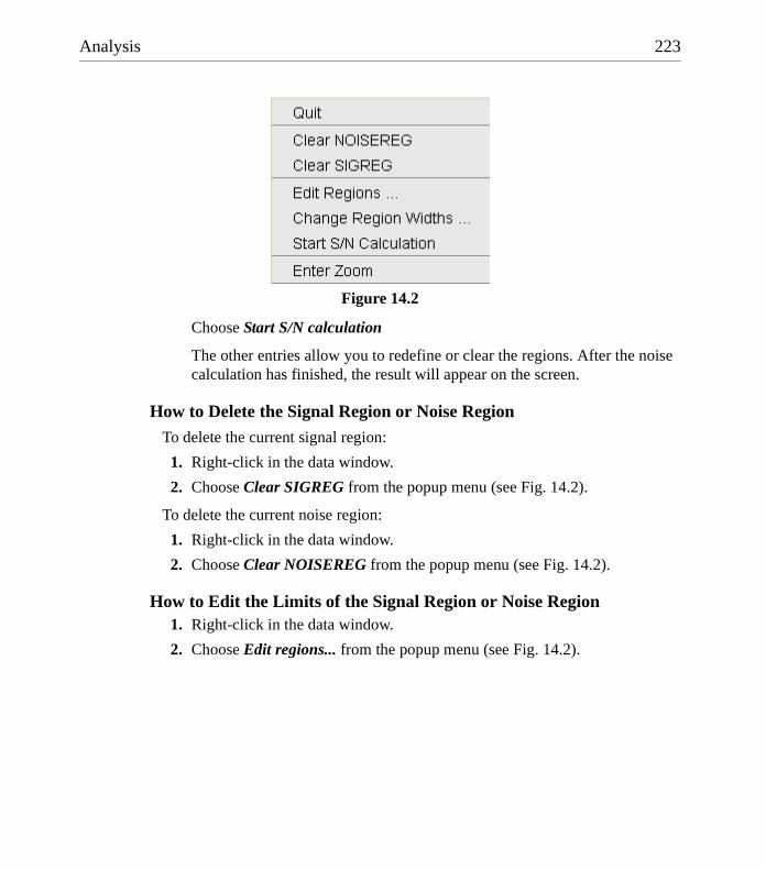
Analysis 223
DONE
INDEX
INDEX
Choose Start S/N calculation
The other entries allow you to redefine or clear the regions. After the noise calculation has finished, the result will appear on the screen.
How to Delete the Signal Region or Noise RegionTo delete the current signal region:
1. Right-click in the data window.
2. Choose Clear SIGREG from the popup menu (see Fig. 14.2).
To delete the current noise region:
1. Right-click in the data window.
2. Choose Clear NOISEREG from the popup menu (see Fig. 14.2).
How to Edit the Limits of the Signal Region or Noise Region1. Right-click in the data window.
2. Choose Edit regions... from the popup menu (see Fig. 14.2).
Figure 14.2
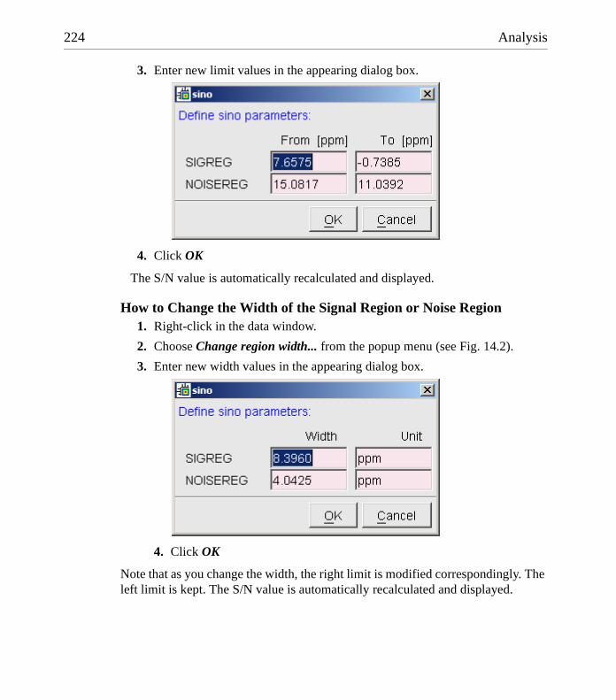
224 Analysis
DONE
INDEX
INDEX
3. Enter new limit values in the appearing dialog box.
4. Click OK
The S/N value is automatically recalculated and displayed.
How to Change the Width of the Signal Region or Noise Region1. Right-click in the data window.
2. Choose Change region width... from the popup menu (see Fig. 14.2).
3. Enter new width values in the appearing dialog box.
4. Click OK
Note that as you change the width, the right limit is modified correspondingly. The left limit is kept. The S/N value is automatically recalculated and displayed.
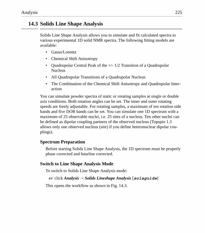
Analysis 225
DONE
INDEX
INDEX
14.3 Solids Line Shape Analysis
Solids Line Shape Analysis allows you to simulate and fit calculated spectra to various experimental 1D solid NMR spectra. The following fitting models are available:
• Gauss/Lorentz
• Chemical Shift Anisotropy
• Quadrupolar Central Peak of the +/- 1/2 Transition of a Quadrupolar Nucleus
• All Quadrupolar Transitions of a Quadrupolar Nucleus
• The Combination of the Chemical Shift Anisotropy and Quadrupolar Inter-action
You can simulate powder spectra of static or rotating samples at single or double axis conditions. Both rotation angles can be set. The inner and outer rotating speeds are freely adjustable. For rotating samples, a maximum of ten rotation side bands and five DOR bands can be set. You can simulate one 1D spectrum with a maximum of 25 observable nuclei, i.e. 25 sites of a nucleus. Ten other nuclei can be defined as dipolar coupling partners of the observed nucleus (Topspin 1.3 allows only one observed nucleus (site) if you define heteronuclear dipolar cou-plings).
Spectrum PreparationBefore starting Solids Line Shape Analysis, the 1D spectrum must be properly phase corrected and baseline corrected.
Switch to Line Shape Analysis Mode
To switch to Solids Line Shape Analysis mode:
! click Analysis " Solids Lineshape Analysis [solaguide]
This opens the workflow as shown in Fig. 14.3.
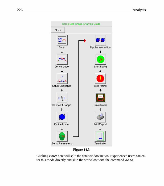
226 Analysis
DONE
INDEX
INDEX
Clicking Enter here will split the data window in two. Experienced users can en-ter this mode directly and skip the workflow with the command sola.
Figure 14.3

Analysis 227
DONE
INDEX
INDEX
The right part of this window is the data window showing the 1D experimental and calculated spectrum. The left part is the parameter window with five panels, where the second one, the Main panel is selected by default.
The simulation procedure
The simulation procedure consists of the following steps:
Set Optional parameters
In the Main panel, you find some parameters which you can normally leave un-changed. See the section Simulation Details below for more information. If a simulation on the current dataset has already been done and stored, you can read this by clicking Open. If not, you will start from scratch and setup the simulation as described below.
Define the Model
Click the Spectrum panel and select the Model according to your experiment. You can refine the experimental conditions by checking one of the following
Figure 14.4

228 Analysis
DONE
INDEX
INDEX
boxes:
• All for all quadrupolar transitions.
• DOR for performed double rotation experiments.
• Sync for rotor synchronized experiments.
When a parameter is greyed, this means it cannot be changed for the se-lected model or it is related to one of the other (checked) parameters.
Define Rotation Parameters
From the Spectrum panel, set the values for:
• MASR - rotation speed of the single axis MAS (VAS) experiments or DOR outer axis speed.
• DORR - inner rotation speed in DOR experiment.
and set their checkmark if they must be optimized during the simulation.
Set the value for:
• SBands: the number of side bands on one side of the central transi-tion.
Define the Spectral Region
Typically, non-overlapping experimental peaks are fitted in separated simula-tions. Before each simulation, the region to which it is applied must be defined.
1. Zoom in on the region to be simulated.
2. Right-click in the data window choosing Define Fitting Region Using Display Region or click DefReg in the panel window.
This will set the parameters F1P and F2P in the Spectrum panel. Alternatively, you can enter the values in the respective parameter fields.
Define Nuclei parameters
For each observable nucleus (site), a set of parameters (see below) must be set. To do that:
1. Click the Nucleus panel or the button.
2. Click Add if the nucleus is not shown yet.
3. Adjust the nuclei parameters until the calculated spectrum approximately fits the experimental spectrum.You can do that as follows:
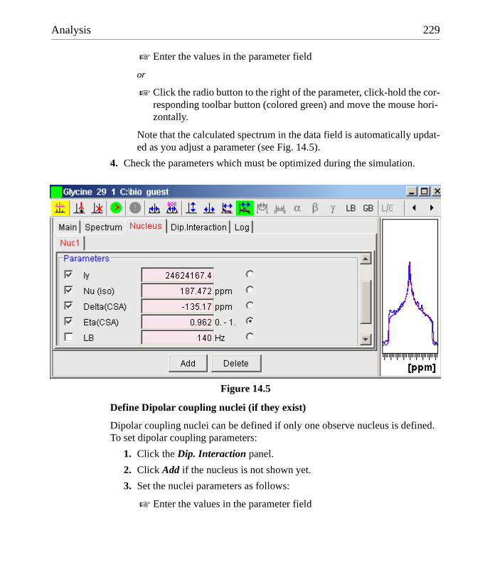
Analysis 229
DONE
INDEX
INDEX
! Enter the values in the parameter field
or
! Click the radio button to the right of the parameter, click-hold the cor-responding toolbar button (colored green) and move the mouse hori-zontally.
Note that the calculated spectrum in the data field is automatically updat-ed as you adjust a parameter (see Fig. 14.5).
4. Check the parameters which must be optimized during the simulation.
Define Dipolar coupling nuclei (if they exist)
Dipolar coupling nuclei can be defined if only one observe nucleus is defined. To set dipolar coupling parameters:
1. Click the Dip. Interaction panel.
2. Click Add if the nucleus is not shown yet.
3. Set the nuclei parameters as follows:
! Enter the values in the parameter field
Figure 14.5
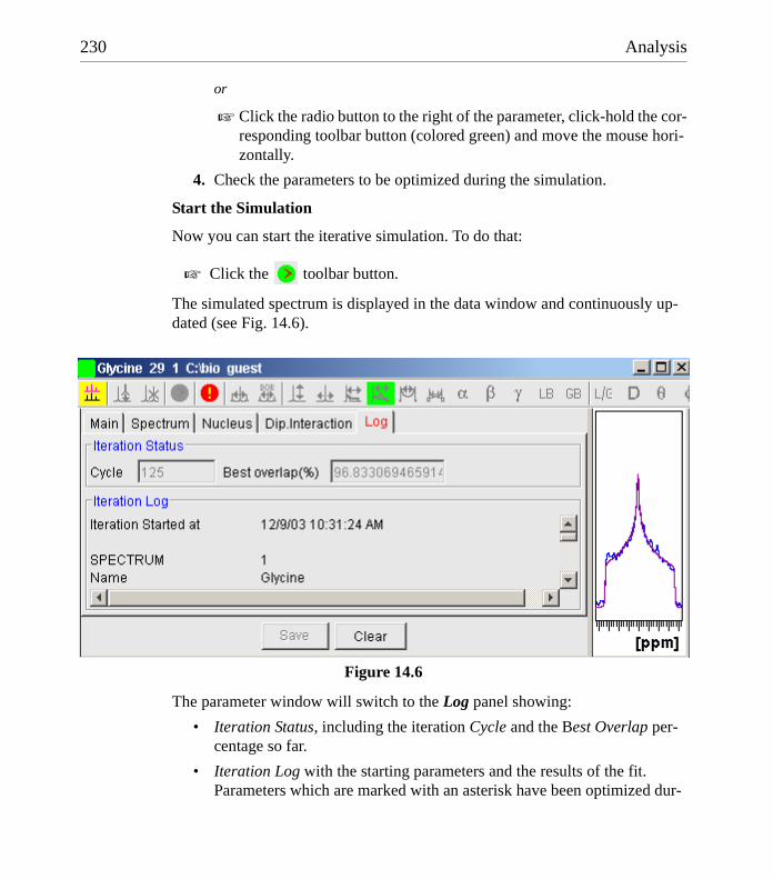
230 Analysis
DONE
INDEX
INDEX
or
! Click the radio button to the right of the parameter, click-hold the cor-responding toolbar button (colored green) and move the mouse hori-zontally.
4. Check the parameters to be optimized during the simulation.
Start the Simulation
Now you can start the iterative simulation. To do that:
! Click the toolbar button.
The simulated spectrum is displayed in the data window and continuously up-dated (see Fig. 14.6).
The parameter window will switch to the Log panel showing:
• Iteration Status, including the iteration Cycle and the Best Overlap per-centage so far.
• Iteration Log with the starting parameters and the results of the fit. Parameters which are marked with an asterisk have been optimized dur-
Figure 14.6

Analysis 231
DONE
INDEX
INDEX
ing the simulation. They are automatically updated in the respective pan-els.
To save the Log panel information, click the Save button.
To clear the Log panel, click the Clear button.
During the simulation process, you can freely switch to other panels to view the parameter being optimized. After the simulation has finished, the Nucleus panel will show the optimized values (see Fig. 14.7).
Abort the Simulation
To abort a running simulation:
! Click the toolbar button.
After a few seconds the iteration stops and the best spectrum will be shown in the data window.
Save the Simulation
After the simulation process is finished for all spectral regions of interest:
1. Switch to the Main panel.
Figure 14.7

232 Analysis
DONE
INDEX
INDEX
2. Click Save
to save all parameters.
Exit Solids Lineshape Analysis
To leave the solids analysis mode:
! Click the toolbar button.
Simulation detailsBasic parameters
The Main panel shows you a list of basic parameters:
• NUCLEUS: the observe nucleus. By default, this parameter is set to the value of the acquisition parameter NUC1.
• SPIN: spin of the observe nucleus. It is automatically set according to the selected NUCLEUS.
• EXPs: number of experimental spectra.
• NUCs: number of nuclei (sites of the observe nucleus).
• DIPs: number of dipolar coupling nuclei.
• TRIANG: number of triangles involved in powder spectrum simulation with several random oriented crystallites. The default value of 32 gener-ally results in a good quality spectrum.
• MAXITER: maximum number of iterations.
• SSIZE: initial step size for the iterated parameters. The value represents the fraction of the initial parameter value. It ranges from 0.0 to 1.0 with a default of 0.1.
The values of NUCs and DIPs will automatically be updated when you add or delete nuclei from the Nucleus and Dip.Interaction panels.
Spectrum parameters
Spc1
TOPSPIN 1.3 supports only one experimental spectrum to be fitted.
Models
Available fitting models are: Gauss/Lorentz, CSA, QUAD central, QUAD all
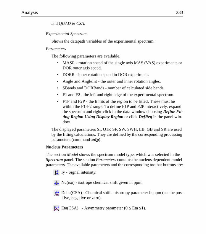
Analysis 233
DONE
INDEX
INDEX
and QUAD & CSA.
Experimental Spectrum
Shows the datapath variables of the experimental spectrum.
Parameters
The following parameters are available.
• MASR - rotation speed of the single axis MAS (VAS) experiments or DOR outer axis speed.
• DORR - inner rotation speed in DOR experiment.
• Angle and AngleInt - the outer and inner rotation angles.
• SBands and DORBands - number of calculated side bands.
• F1 and F2 - the left and right edge of the experimental spectrum.
• F1P and F2P - the limits of the region to be fitted. These must be within the F1-F2 range. To define F1P and F2P interactively, expand the spectrum and right-click in the data window choosing Define Fit-ting Region Using Display Region or click DefReg in the panel win-dow.
The displayed parameters SI, O1P, SF, SW, SWH, LB, GB and SR are used by the fitting calculations. They are defined by the corresponding processing parameters (command edp).
Nucleus Parameters
The section Model shows the spectrum model type, which was selected in the Spectrum panel. The section Parameters contains the nucleus dependent model parameters. The available parameters and the corresponding toolbar buttons are:
Iy - Signal intensity.
Nu(iso) - isotrope chemical shift given in ppm.
Delta(CSA) - Chemical shift anisotropy parameter in ppm (can be pos-itive, negative or zero).
Eta(CSA) - Asymmetry parameter (0 ≤ Eta ≤1).
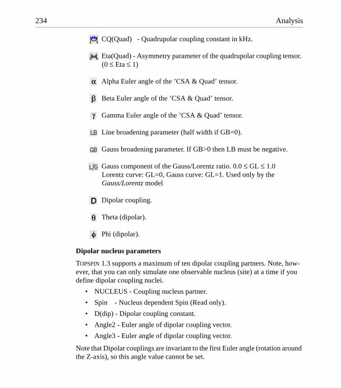
234 Analysis
DONE
INDEX
INDEX
CQ(Quad) - Quadrupolar coupling constant in kHz.
Eta(Quad) - Asymmetry parameter of the quadrupolar coupling tensor. (0 ≤ Eta ≤ 1)
Alpha Euler angle of the ’CSA & Quad’ tensor.
Beta Euler angle of the ’CSA & Quad’ tensor.
Gamma Euler angle of the ’CSA & Quad’ tensor.
Line broadening parameter (half width if GB=0).
Gauss broadening parameter. If GB>0 then LB must be negative.
Gauss component of the Gauss/Lorentz ratio. 0.0 ≤ GL ≤ 1.0Lorentz curve: GL=0, Gauss curve: GL=1. Used only by the Gauss/Lorentz model
Dipolar coupling.
Theta (dipolar).
Phi (dipolar).
Dipolar nucleus parameters
TOPSPIN 1.3 supports a maximum of ten dipolar coupling partners. Note, how-ever, that you can only simulate one observable nucleus (site) at a time if you define dipolar coupling nuclei.
• NUCLEUS - Coupling nucleus partner.
• Spin - Nucleus dependent Spin (Read only).
• D(dip) - Dipolar coupling constant.
• Angle2 - Euler angle of dipolar coupling vector.
• Angle3 - Euler angle of dipolar coupling vector.
Note that Dipolar couplings are invariant to the first Euler angle (rotation around the Z-axis), so this angle value cannot be set.

Analysis 235
DONE
INDEX
INDEX
The Simplex algorithm
The Simplex iteration minimizes the least square difference of the experimental spectrum and the superimposed simulated spectra between F1P and F2P. The ’Best overlap %’ value is determined as described below.
Calculate the area between the curves of the experimental and the calculated spectra.
A(dif) = Sum(Abs(Yexp(i)-Ycalc(i)))
Calculate the area of the experimental spectrum.
A(exp) = Sum(Abs(Yexp(i)))
Compare these to area values.
Overlap(%) = 100*(1-A(dif)/A(exp))
Overlap(%) = 100, if A(dif)=0. This is the theoretical maximum of the signal overlap.
Overlap(%) = 0, if the calculated spectrum is similar to the experimental one, with same area, but they do not overlap.
Overlap(%) > 0, but <100. Partial overlap.
Overlap(%) > 70-90, good agreement.
Overlap < 0. No agreement. Change the initial parameters and start a new sim-ulation.
14.4 Relaxation Analysis
Typically, relaxation data consist of a series of 1D FIDs measured with varying delays and stored as pseudo 2D data. To analyze these data, Topspin offers an easy to use T1/T2 Relaxation Guide. Relaxation curves of various experiment types with up to six components can be fitted.
To start the Relaxation Guide:
! Click Analysis " T1/T2 Relaxation [t1guide].
This will open the dialog box as shown in Fig. 14.8.
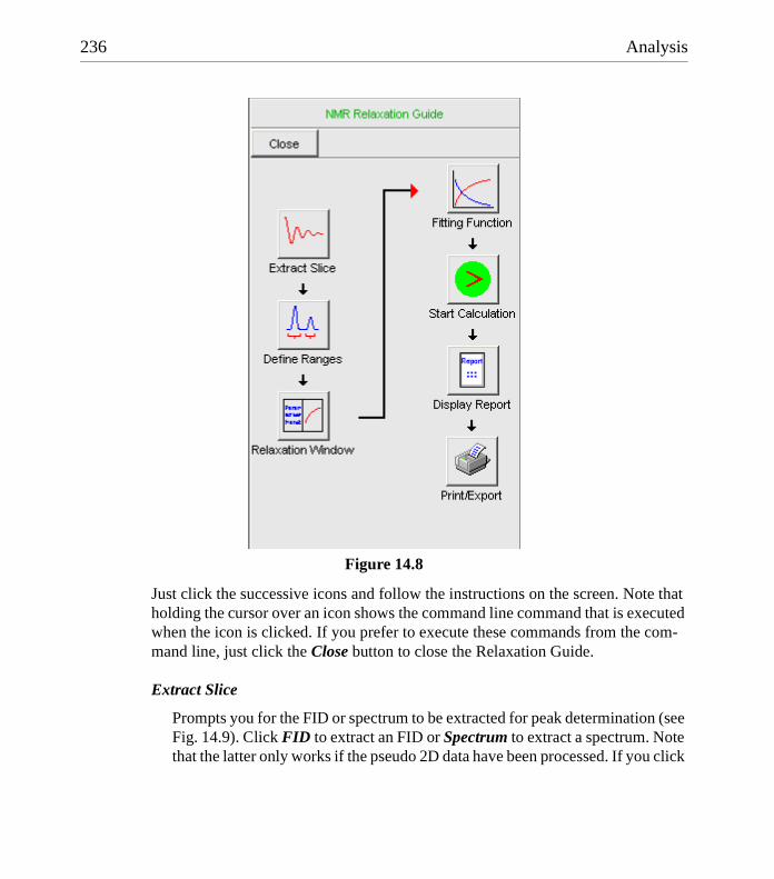
236 Analysis
DONE
INDEX
INDEX
Just click the successive icons and follow the instructions on the screen. Note that holding the cursor over an icon shows the command line command that is executed when the icon is clicked. If you prefer to execute these commands from the com-mand line, just click the Close button to close the Relaxation Guide.
Extract Slice
Prompts you for the FID or spectrum to be extracted for peak determination (see Fig. 14.9). Click FID to extract an FID or Spectrum to extract a spectrum. Note that the latter only works if the pseudo 2D data have been processed. If you click
Figure 14.8

Analysis 237
DONE
INDEX
INDEX
FID, the extracted FID is automatically processed. We recommend to enter the
FID or spectrum number which was measured with the longest delay. It can be found in the vdlist file in the EXPNO data directory. A new data window will appear, showing the extracted 1D-FID.
Transform/Phase
Processes the extracted 1D FID performing exponential multiplication, Fourier transform and automatic phase correction.
Define Ranges
Switches to interactive integration mode. Here you can define the ranges for the peaks to be included in the relaxation analysis.
1. Click the button in the data window toolbar.
2. Put the red cursor line at one edge of a peak or multiplet.
3. Left-click-hold and drag the cursor line to the other edge of the peak or multiplet.
4. Do step 2 and 3 for all regions to be defined.
5. Click the button and choose Export Regions to Relaxation Module
6. Click to return [.ret].
Relaxation Window
Switches the 1D data window to relaxation analysis mode (see Fig. 14.10)
Figure 14.9

238 Analysis
DONE
INDEX
INDEX
and performs a default fitting. By default, this is one-component, T1-intensity fitting (Function type uxnmrt1) for peak 1. If the dataset was already fitted, the previous type of fitting is performed. The fitting curve is displayed in the data section and a Brief Report is shown in the parameter section. If this default fit-ting is appropriate, you can view, interpret and print the results as described be-low. If not, you can perform the desired fitting as described below.
Perform Fitting and Calculate the Relaxation Time
Depending on the experiment, you can perform the appropriate fitting as fol-lows:
1. Select a Fitting type: Intensity or Area. Either every point reflects the intensity of the biggest peak in the defined integral range or the integral itself. Both of them can be used but, depending on the experiment, one of them usually give a better fitting curve.
2. Click the button to open the parameter dialog box. Select a Func-tion Type and set the required parameters (see below). Click OK.
ES
Figure 14.10

Analysis 239
DONE
INDEX
INDEX
3. Perform fitting and calculate the relaxation time:
Fit the relaxation curve for the current peak.
Fit the relaxation curve for all peaks.
View and interpret the results as described below.
Function Types and Parameters
The TOPSPIN relaxation routine offers functions for various relaxation experi-ments with up to 6 components:
uxnmrt1 for one-component T1 experiments. Set the parameter List file name to the list type used during the acquisition. The T1 fitting function is defined by the function:
where I is Intensity or Area according to the Fitting Type. The best fit is cal-culated by varying I(0), P and T1 in an iterative process according to the Lev-enberg-Marquardt algorithm. Clicking and executes the commands ct1 (current peak) and dat1 (all peaks), respectively.
uxnmrt2 for one-component T2 experiments. Set the parameter List file name to the list type used during the acquisition. A T2 fitting function is de-fined by the function:
where I is Intensity or Area according to the Fitting Type. The best fit is cal-culated by varying P and T2 in an iterative process according to the Leven-berg-Marquardt algorithm. Clicking and executes the commands ct2 (current peak) and dat2 (all peaks), respectively.
invrec, satrec, cpt1rho, expdec, gaussdec, lorgauss linear, varbigdel, var-litdel, vargrad, vardamp: these functions can be used for various experi-ments with up to 6 components, except for cpt1rho and lorgauss which allow only 4 and 3 components, respectively. They all use the simplex algo-rithm and require some parameters to be set:
• Enter the Number of components
I t( ) I 0( ) Pt
T1------ exp×+=
I t( ) Pt
T2------ exp×=

240 Analysis
DONE
INDEX
INDEX
• Click the Setup button to set the Iteration Control parameters. For each component, the initial guess (G) and step rate (S) can be set. The initial guess for I[0] must be selected such that the sum of all compo-nents does not exceed 1. If there is only one component, I[0] is usu-ally set to 1.The step rate is usually set to about one tenth of the initial guess. If the step rate of a variable is set to zero, then this variable is not changed during the iterations.
Clicking and executes the commands simfit (current peak) and simfit all (all peaks), respectively.
View the Fitting Results
When the fitting procedure has finished, the fitting curve is displayed in the data section and a Brief Report appears in the parameter section (see Fig. 14.10). The latter consists of:
• the calculated relaxation value
• the fitted parameters
• the standard deviation SD
For further examination of the result, click one of the following buttons:
Show the fitting result of the previous peak/area.
Show the fitting result of the next peak/area.
Switch x-axis to linear scaling.
Switch x-axis to logarithmic scaling.
Switch x-axis to quadratic scaling.
Export integrals to dataset ~TEMP and exit.
Show an extended report, including the fitted intensity or area distribu-tion. This consists of the same information as the brief report plus a ta-
ble with the intensity or area distribution. Example:
Dataset : C:/bio/data/guest/nmr/t1test/1/pdata/1
INTENSITY fit :
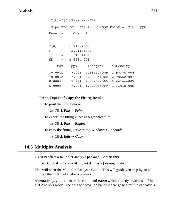
Analysis 241
DONE
INDEX
INDEX
I[t]=I[0]+P*exp(-t/T1)
12 points for Peak 1, Cursor Point = 7.221 ppm
Results Comp. 1
I[0] = 1.215e+000P = -2.211e+000T1 = 19.449sSD = 3.685e-003
tau ppm integral intensity
30.000s 7.221 2.5811e+009 1.9737e+00810.000s 7.221 -3.2898e+008 -2.9056e+0078.000s 7.221 -7.8525e+008 -6.4616e+0075.000s 7.221 -1.6289e+009 -1.3101e+008
...
Print, Export of Copy the Fitting Results
To print the fitting curve:
! Click File " Print
To export the fitting curve as a graphics file:
! Click File " Export
To copy the fitting curve to the Windows Clipboard:
! Click Edit " Copy
14.5 Multiplet Analysis
TOPSPIN offers a multiplet analysis package. To start this:
! Click Analysis " Multiplet Analysis [managuide].
This will open the Multiplet Analysis Guide. This will guide you step by step through the multiplet analysis process.
Alternatively, you can enter the command mana which directly switches to Multi-plet Analysis mode. The data window Tab bar will change to a multiplet analysis

242 Analysis
DONE
INDEX
INDEX
toolbar. Fig. 14.11 shows a region of an ethanol spectrum.
Multiplet analysis can be performed in three different ways:
• define multiplet by region
• define multiplet manually
• define multiplet by free grid
For multi-level multiplets, the following methods are available:
• couple existing multiplets into a multi-level multiplet
• define multi-level multiplet by coupled grid
Multiplet analysis uses a maximum intensity search within a user-defined capture range (see Fig. 14.18). If peak picking has been performed (required for defining a multiplet by region), the found peaks within the capture range are used. However, only peaks with the defined minimum intensity are used (see Fig. 14.18).
The three methods are described here for the ethanol CH3, OH and CH2 group, respectively. You can use one of these methods, depending on the type of spectrum and your own preference. In this example, the chosen methods for each group is arbitrary.
14.5.1 Define multiplet by region
In this mode, you simply define the region around the multiplet. The multiplet is
Figure 14.11
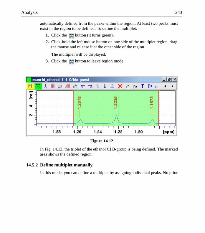
Analysis 243
DONE
INDEX
INDEX
automatically defined from the peaks within the region. At least two peaks must exist in the region to be defined. To define the multiplet:
1. Click the button (it turns green).
2. Click-hold the left mouse button on one side of the multiplet region, drag the mouse and release it at the other side of the region.
The multiplet will be displayed.
3. Click the button to leave region mode.
In Fig. 14.13, the triplet of the ethanol CH3-group is being defined. The marked area shows the defined region.
14.5.2 Define multiplet manually.
In this mode, you can define a multiplet by assigning individual peaks. No prior
Figure 14.12
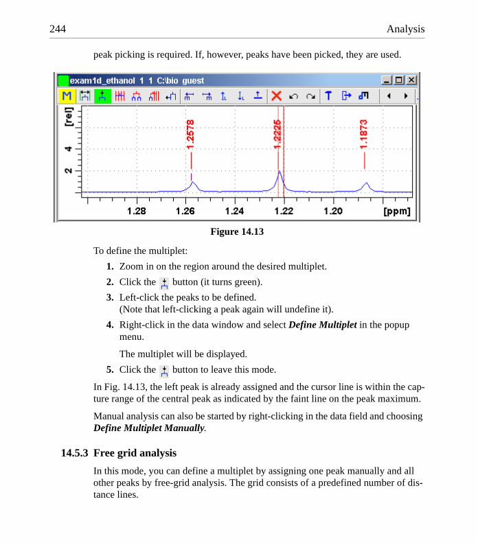
244 Analysis
DONE
INDEX
INDEX
peak picking is required. If, however, peaks have been picked, they are used.
To define the multiplet:
1. Zoom in on the region around the desired multiplet.
2. Click the button (it turns green).
3. Left-click the peaks to be defined.(Note that left-clicking a peak again will undefine it).
4. Right-click in the data window and select Define Multiplet in the popup menu.
The multiplet will be displayed.
5. Click the button to leave this mode.
In Fig. 14.13, the left peak is already assigned and the cursor line is within the cap-ture range of the central peak as indicated by the faint line on the peak maximum.
Manual analysis can also be started by right-clicking in the data field and choosing Define Multiplet Manually.
14.5.3 Free grid analysis
In this mode, you can define a multiplet by assigning one peak manually and all other peaks by free-grid analysis. The grid consists of a predefined number of dis-tance lines.
Figure 14.13

Analysis 245
DONE
INDEX
INDEX
To define the multiplet:
1. Zoom in on the region around the desired multiplet.
2. Click the button (it turns green).
3. Right-click in the data window and, if necessary, set the number of distance lines.
4. Left-click the central peak to be defined. For a multiplet with an even number of peaks, left-click one of the central peaks. The central peak will be marked. Note that clicking a marked peak again will unmark it.
5. Move the mouse to the left or right until the grid lines coincide with the remaining multiplet peaks and click the left mouse button.The multiplet will be displayed.
6. Click the button to leave this mode.
In Fig. 14.14, the triplet of the ethanol OH-group is being defined. The central peak is defined and the black grid lines are in the capture range of the other peaks as shown by the faint lines on the peak maxima.
14.5.4 Couple existing Multiplets into a Multi-level Multiplet
In this mode, you can defined a multi-level multiplet by coupling already defined multiplets. To do that:
Figure 14.14
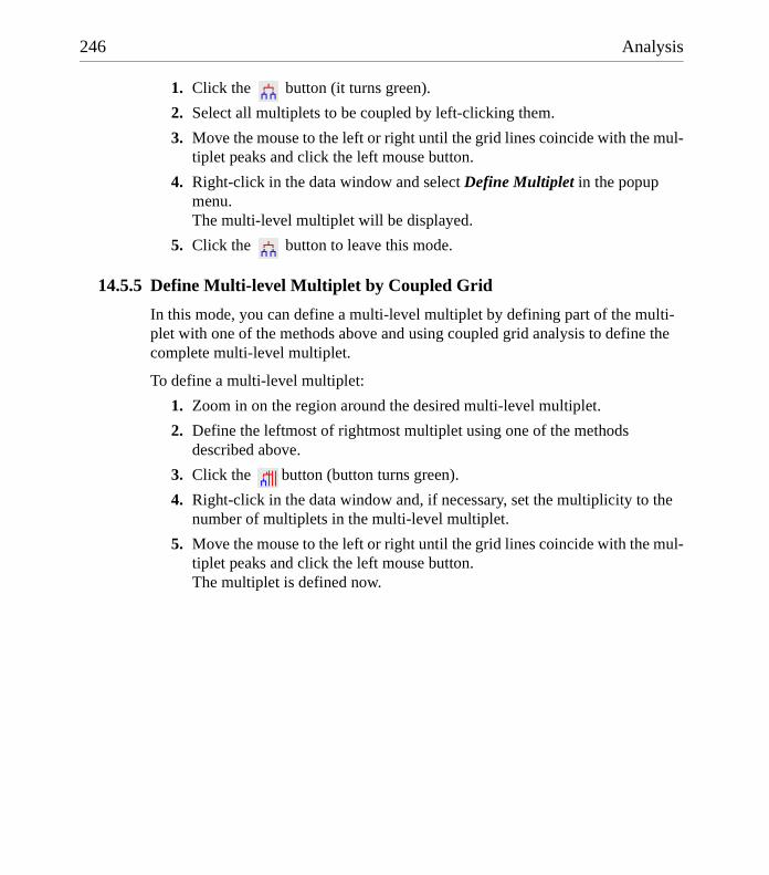
246 Analysis
DONE
INDEX
INDEX
1. Click the button (it turns green).
2. Select all multiplets to be coupled by left-clicking them.
3. Move the mouse to the left or right until the grid lines coincide with the mul-tiplet peaks and click the left mouse button.
4. Right-click in the data window and select Define Multiplet in the popup menu.The multi-level multiplet will be displayed.
5. Click the button to leave this mode.
14.5.5 Define Multi-level Multiplet by Coupled Grid
In this mode, you can define a multi-level multiplet by defining part of the multi-plet with one of the methods above and using coupled grid analysis to define the complete multi-level multiplet.
To define a multi-level multiplet:
1. Zoom in on the region around the desired multi-level multiplet.
2. Define the leftmost of rightmost multiplet using one of the methods described above.
3. Click the button (button turns green).
4. Right-click in the data window and, if necessary, set the multiplicity to the number of multiplets in the multi-level multiplet.
5. Move the mouse to the left or right until the grid lines coincide with the mul-tiplet peaks and click the left mouse button.The multiplet is defined now.
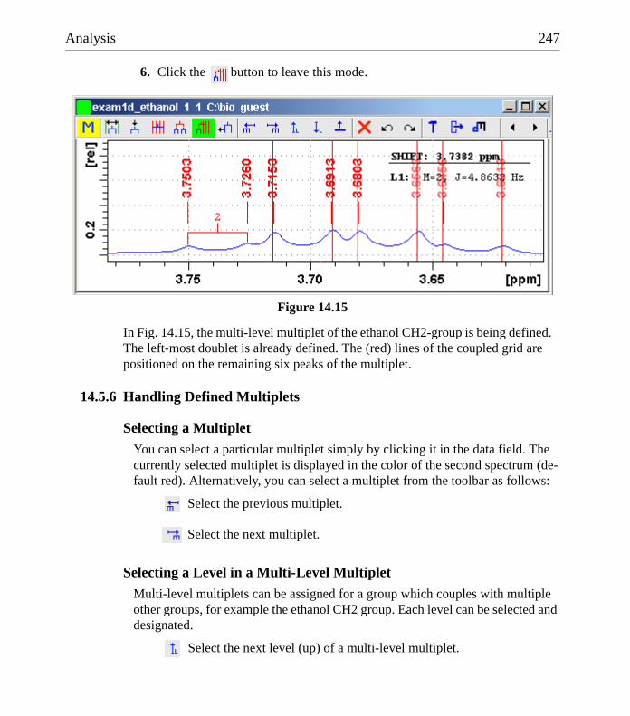
Analysis 247
DONE
INDEX
INDEX
6. Click the button to leave this mode.
In Fig. 14.15, the multi-level multiplet of the ethanol CH2-group is being defined. The left-most doublet is already defined. The (red) lines of the coupled grid are positioned on the remaining six peaks of the multiplet.
14.5.6 Handling Defined Multiplets
Selecting a MultipletYou can select a particular multiplet simply by clicking it in the data field. The currently selected multiplet is displayed in the color of the second spectrum (de-fault red). Alternatively, you can select a multiplet from the toolbar as follows:
Select the previous multiplet.
Select the next multiplet.
Selecting a Level in a Multi-Level MultipletMulti-level multiplets can be assigned for a group which couples with multiple other groups, for example the ethanol CH2 group. Each level can be selected and designated.
Select the next level (up) of a multi-level multiplet.
Figure 14.15

248 Analysis
DONE
INDEX
INDEX
Select the previous level (down) of a multi-level multiplet.
Designating a Level in Multi-Level MultipletsA level of a multi-level multiplet can be designated to connect with another mul-tiplet. To do that:
! Right-click in the multiplet and choose Designate Multiplet
The designated level is displayed in the color of the fourth spectrum (default pur-ple). Note that the selected level can be different from the designated level.
14.5.7 Define Multiplet Identifiers
To define multiplet identifiers:
1. Left-click the multiplet.
2. Right-click the multiple and select Define Multiplet Identifier in the popup menu.
3. Specify the multiplet identifier in the appearing dialog and click OK
Alternatively, multiplet identifiers can be defined by clicking the button and double-clicking the respective multiplet lines in the appearing Report dialog. This will open the Identifier dialog (see Fig. 14.16). Just fill out the field Identifier and click OK.

Analysis 249
DONE
INDEX
INDEX
Note that the dialog also offers a button to Disconnect the current multiplet and a field Connection that shows all possible connections using the follow-ing flags:
& : the current connection
# : a non-existing connection
! : a different existing connection
14.5.8 Define Multiplet Connections
Once the multiplets of a spectrum are defined, you can define the connections between them.
To define all connections: 1. Click the button to see the Report dialog (see Fig. 14.17).
Figure 14.16

250 Analysis
DONE
INDEX
INDEX
2. The multiplets appear in the order in which they have been defined.
Newly defined multiplets appear with numbers as ID’s and no multiplet con-nections (x,0) defined.
3. Click the button Find Connections to make the multiplet connections:
a) Set the maximum difference between related couplings or accept the default.
b) Set the lower limit for couplings or accept the default.
c) Check the box Change already defined Connections if applicable.
d) Click OK to define the connections.
Note that the Report Dialog also offer buttons for Printing the multiplet informa-tion, copying it to the clipboard and saving it to a text file.
To define individual connections: 1. Select the first multiplet. In case of a multi-level multiplet, click the or
button to select the required level.
Figure 14.17

Analysis 251
DONE
INDEX
INDEX
2. Right-click and select Designate Multiplet from popup menu.
3. Select the second multiplet. In case of a multi-level multiplet, click the or button to select the required level.
4. Right-click and choose the Connect Multiplets from popup menu.
To define individual connections:
To disconnect multiplets: 1. Select on of the multiplets to be disconnected.
2. Right-click and select Disconnect Multiplets from popup menu.Shifting a Multiplet Line
Alternatively, you can open disconnect a multiplet from the Identifier dialog (see Fig. 14.16)
14.5.9 Further Multiplet Functions
The Multiplet Analysis window offers several other function such as:
Shift multiplet line. Click this button and move the vertical cursor line into the capture area of the desired line which is then marked by a faint line. The left-click-hold and move the moos to the desired position.
Shift multiplet vertically. Click this button and move the mouse to put the horizontal line cursor above or below the multiplet tree. Then left-click to shift the multiplet to that position.
Remove the currently selected multiplet. Clicking this button several times allows you to remove all multiplets.
Show Daisy multiplets.
Undo the last multiplet action.
Redo the last multiplet action.
14.5.10 How to Set Multiplet Options
The button opens a dialog box where you can set various multiplet options as

252 Analysis
DONE
INDEX
INDEX
shown in Fig. 14.18.
• Distance lines: the default number of distance lines in the multiplet dialogs.
• Capture range: the search range for maximum intensity of peak position in manual mode.
• Drift range: the maximum difference in data points between line distances within one multiplet
• Min. Intensity: The minimum intensity of a peak compared to the reference peak to be accepted as a multiple line.
• Min. Delta/J: the minimum ratio of the difference in chemical shift of the coupling groups and the coupling constant. Below this value, the coupling constant in the Report box is indicated with a question mark to suggest pos-sible second order effect.
• Labels Vertical: displays multiplet labels 90° rotated.
All toolbar functions are also available from a popup menu which appears when you right-click in the data window (see Fig. 14.19).
Figure 14.18
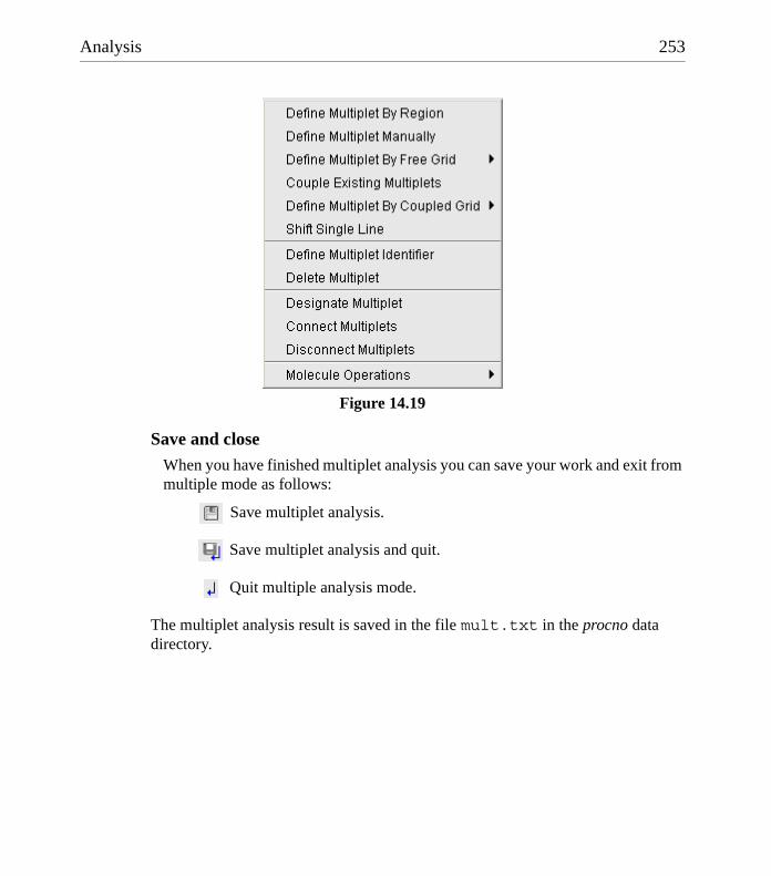
Analysis 253
DONE
INDEX
INDEX
Save and closeWhen you have finished multiplet analysis you can save your work and exit from multiple mode as follows:
Save multiplet analysis.
Save multiplet analysis and quit.
Quit multiple analysis mode.
The multiplet analysis result is saved in the file mult.txt in the procno data directory.
Figure 14.19


I-1
Index
Symbols
*2 command 31, 37, 104, 135*8 command 31, 104, 135.2d command 30.3d command 30.all command 32, 105, 137.basl command 182.bmp files 22.bzip files 23, 66.cal command 174.co command 148.dec command 164, 169, 185, 199.dopt command 127.dx files 66.emf files 22.f1r command 137.f2r command 137.gif files 339.gr command 147.hr command 32, 105.hz command 124, 144.im command 151.inc command 164, 169, 185, 199.int command 165.jpeg files 22, 339.jpg files 22, 339.keep command 32, 105, 137.ls command 151.lt command 153.lv command 149.md command 21, 175.ov command 125, 144.ph command 39, 161, 193.ph180 command 163.ph90 command 163.phr command 163.png files 22, 99, 339.pp command 188
.pr command 21, 145
.prop files 54, 218
.ret command 164, 173, 182, 185, 187, 191
.retsab command 187
.s2d command 164
.sd command 33, 106, 137
.sino command 222
.sl command 32, 106, 137
.sl0 command 32, 106
.sr command 32, 106, 137
.sr0 command 32, 106
.sret command 164, 173, 185, 191
.st command 151
.su command 33, 106, 137
.tif files 99
.txt files 130
.vr command 32, 104, 135
.wmf files 22, 99
.y command 125
.zi command 32, 105, 136
.zl command 32, 105, 137
.zo command 32, 105, 136
.zx command 32, 105, 136/2 command 31, 37, 104, 135/8 command 31, 104, 135? command help 40
Numerics
180 degree phase correction1D 1632D 199
-90 degree phase correction1D 1632D 199
90 degree phase correction1D 1632D 199

I-2
DONE
INDEX
INDEX
A
abs command 87, 90, 164, 165, 167, 182absd command 182absorption mode 162, 163, 197, 198, 199acqu command 258acquisition
commands 258, 260mode 301parameters 82, 83, 269status bar 259, 271toolbar 257
Acquisition Reference Manual 19, 85, 264, 265, 302AcquPars tab 82, 108, 140, 269activate
a data window 213the next data window 218
addcomment to audit file 77data to portfolio 74directory to the browser 20, 53found data to portfolio 54, 74functionalities to Topspin 25peak in 2D phase correction 194peak to peak list 190
add increment in 2D levels 149align
intensities in multiple display 180peak positions in multiple display 180
Alt-F11 key 104, 134Alt-F4 key 36, 41Alt-F6 key 41Analysis menu 23, 29anisotropy 225apk command 87, 90, 161apks command 161arrange
data windows 214data windows horizontally 216data windows vertically 215rows/columns in 2D phase correction 200
ascii files 75, 130ased command 84, 108Aspect 3000 data 65ATM probehead 261, 262atma command 262
AU macros 25, 332, 333AU program reference manual 91AU programs 19, 25, 90, 303, 332, 336, 339audit
trail check 76trail files 76
audit command 76auditp.txt file 76automate data acquisition 26automatic
1D baseline correction 871D calibration 87, 1731D integration 1641D peak picking 1871D phase correction 87, 1612D calibration 206compilation of an AU program 304configuration of a datastation 301selection of the first expno/procno 60startup actions 317tuning and matching 262
automatic modeof the Acquisition Guide 256of the Processing Guide 23, 88
automation 25, 26, 303autoplot command 90, 96autostart.prop file 316Avance spectrometers 16, 301axis units 31, 124, 144, 175, 207
B
background of a data window 320Backspace key 33backward peak picking 190baseline correction
1D 87, 182mode 30, 182
bcm command 185bias correction 168bio-molecular experiments 26bnmr command 334bnmrsel command 334bpan command 335browser 27, 28, 36, 49, 59
font 323

I-3
DONE
INDEX
INDEX
in multiple display mode 177, 202Bruker
AU programs 25, 303data format 19, 23, 24, 62, 65, 66, 74example datasets 20, 53
BSMS control panel 264BSMS display window 218bsmsdisp command 264
C
calibration 871D interactive 1732D interactive 206mode 30, 173, 206
cf command 18, 43, 299, 300, 301chemical shift 180chemical shift distance
1D 2212D 208
CHEMSTR parameter 122C-language 25, 90, 332, 333clevels file 151clipboard 22, 36close
active data window 217lock display window 263, 264the active data window 36wobble window 262
close button 29close command 36cmdhist command 34cmdindex command 40cmdtab_user.prop file 41collapse a data directory 49, 52color scheme 320colors
of data objects 319of the lock display 319on the printer 319
commandaudit 76definition 41dialog box 79help 39index 40
line 33, 34, 324command line
commands 258focus 33, 36font 324history 33, 34preferences 324resize 325usage 33
Command Prompt 18, 300compile
AU program 304components
of a spectrum 22composite commands 88configuration
commands 18customized 301default 301directory 301name 301of a datastation 18of a spectrometer 18of the acquisition status bar 259of the tab bar 318of the Topspin menu 327password 299
consistency check 76contour display 194
of 2D spectra 148of 3D planes 156
contour levels 134, 149control keys 36convdta command 67conventions in this document 15convert
data to JCAMP-DX 67data to text 67data to ZIP 67
copy & paste data 29, 64, 66copy command 22, 30, 99copy data 66C-program 90create
an AU program 25, 91, 304, 332
I-4
DONE
INDEX
INDEX
an empty data window 59data window color scheme 320dataset 30macro 25, 332new data window 19new dataset 56, 268plot layouts 22, 97Python program 26, 333set of user preferences 315user defined command 25user notebook 331
C-statements 25Ctrl key 52, 54, 60, 71, 74, 104, 135, 176, 178Ctrl-c key 33, 36, 114Ctrl-d key 27, 36, 51Ctrl-f key 36Ctrl-F3 key 41Ctrl-F5 key 41Ctrl-F6 key 41Ctrl-n key 30, 36, 56, 268Ctrl-o key 30, 36, 61, 65Ctrl-p key 22, 30, 36, 97, 114Ctrl-s key 23, 30, 36, 67, 68Ctrl-v key 34, 36Ctrl-w key 36cube display 155cubic spline baseline correction 185cursor information 127customized configuration 301cut integrals 172
D
dataarea 20, 27, 59, 64, 66, 211, 214, 217compression 24dimensionality 28, 81, 84, 108directory 49, 53, 71field 33, 101, 106, 133object colors 319
data window 19, 27, 29, 59, 64, 662D 1333D 155color scheme 320contents 22, 99creation 59
handling 29, 211in 1D peak picking mode 188in 1D phase correction 162in 2D calibration mode 207in 2D multiple display mode 201in 2D phase mode 194in baseline correction mode 183in calibration mode 174in integration mode 165in multiple display mode 177in S/N measurement mode 222in spline baseline correction mode 186objects 22popup menu 126, 138printing 95reopen 102tab bar 1D 106tab bar 2D 139tab bar 3D 159toolbar 21
datasetactive 213colors 182dir 19directory tree 19, 63expno 19, 50, 56files 75, 130handling 25, 49last 2D 30last 3D 30last used 317name 19, 50, 56, 64procno 19, 50, 56procno directory 63properties 73, 128selection in multiple display 178specification 63, 213title 57top level directory 50user 19, 50, 56variables 68
datastationconfiguration 301
dcon command 24, 328dconpeaks.txt file 24
I-5
DONE
INDEX
INDEX
deconvolution 24default
color scheme 320command line size 324configuration 301find criteria 72menu font 322pivot point in 1D phase correction 162pivot point in 2D phase 197plane in 3D display 155printer 96Tab bar 318zero order phase correction 163
definecubic spline baseline points 185integral regions 166NMR ADMINISTRATOR password 299NMR SUPERUSER 299peak ranges 188peaks 190
de-iconifydata window 217
deleteAU program 304data 68integrals from display 170noise region S/N 223peaks from a peak list 190signal region S/N 223spline baseline points 186
Delete key 33depth cueing in 3D 159deselect
data in multiple display 178integral regions 166
dialog box font 323difference spectrum
in baseline correction 184in multiple display 179
dimensionality of a dataset 28, 81, 82, 84, 108dipolar coupling 229dir command 20disable
commands 326menus 326
toolbar buttons 326Display
button 19, 65, 73menu item 59, 176
display1D acquisition status parameters 1081D data 1011D FID 1241D integral list 1151D peak list 1101D processed data 1071D raw data 1241D spectrum 1071D spectrum overview 1242D contours 1482D data 1332D FID 1432D grid 1472D integral list 1422D peak list 1412D projections 1452D spectrum in contour mode 1482D spectrum in image mode 1512D spectrum in oblique mode 1513D cube 1573D data 155columns in 2D phase correction 194contours in 2D phase 194data from the browser 20, 60data from the portfolio 60data in multiple windows 102dataset file list 128dataset properties 128expno/procno list 60found dataset 73full spectrum in 2D phase correction 195integrals 20JCAMP data 24manipulation 103manipulations 31mode of the lock window 263molecule structure 122options 31options 1D 124peaks 20

I-6
DONE
INDEX
INDEX
planes of 3D data 155, 156positive/negative 2D levels 153processing status parameters 1D 108projections 21rows in 2D phase correction 194settings 30special data formats 65spectra 19spectrum overview in 2D 144status parameters 81, 84sum/difference spectrum 179superimposed 1D spectra 175superimposed 2D spectra 200y-axis 31, 125zipped data 23
display properties 21distance measurement
1D 2212D 208mode 31
DORR parameter 228double rotation experiments 228double-headed arrow 212, 222Down-Arrow key 33, 37dpa command 108dpp command 81, 84, 108drag & drop data 64, 66
E
eda command 82, 83, 108, 140edasp command 85edau command 25, 91, 303, 304, 332edcpul command 109edit
AU program 304commands 34contour levels 149integral ranges 168pulse program 109signal/noise regions 223title of a dataset 109
Edit menu 29edlev command 134, 149edlock command 85edmac command 25, 332
edp command 23, 79, 80, 107, 140edprosol command 84edpy command 26, 333edti command 109ef command 88, 90efp command 88, 271em command 23, 87email data 24empty data window 59enable
disabled commands 328menus/commands 325
Enter key 37, 60equidistant sequence of levels 149Esc key 33Euler angle 234execute
AU program 303, 304macro 25, 332Python program 26
exit command 36, 42expand
a data directory 37data directory 19, 20, 49data directory fully 52data directory in the browser 52individual spectra in multiple display 180spectrum 24
experiment time 258expinstall command 18, 43, 258, 299, 300, 301, 303expl command 63, 75, 76, 130Explorer 49, 63, 75, 130expno 56, 60, 63, 68, 128exponential
baseline correction 184window multiplication 87, 88
export data 22, 99expt command 258extend the Topspin functionality 331external projection 21extract a row/column in 2D 205
F
F1 dimension 137, 144, 193F1 key 15, 36

I-7
DONE
INDEX
INDEX
F1-F2 plane 156, 159F2 dimension 137, 144, 193F2 key 36, 51F2-F3 plane 157, 159F3 key 41F3-F1 plane 155, 157, 159F5 key 41F6 key 36, 41, 214FDA 76fid command 124, 143FID display 258, 260, 266, 269Fid tab 124, 128, 143File Chooser 19File menu 19, 29file size of raw data 258files of a dataset 64, 67, 75, 128, 130find command 36, 54, 71find data 29, 54, 71first order phase correction
1D 1632D 197, 198
fitting peaks 24fmc command 88focus 33, 36, 51font
of dialog windows 323of the browser 323of the command line 324of the interface 321of the menu 322of the status line 324of the tab bar 322
forward peak picking 190Fourier transform 87, 88fp command 88fromjdx command 24fromzip command 23ft command 23, 87ftf command 23, 327function keys 36
G
Gaussian deconvolution 24Gaussian window multiplication 88genfid command 67, 68
genser command 68geometric sequence of levels 149geometry of a Topspin window 218, 219getprosol command 84, 108gf command 88gfp command 88GLP 76GMP 76Gnome Mozilla 76grab rows/columns in 2D 204gradient enhanced spectroscopy 25graphic functions 333graphics files 22, 99grid
display 31, 147, 263window arrangement 214
gs command 82, 266GS parameter adjustment window 266
H
halt an acquisition 258, 259halt command 258, 270helium level 264Help
button 40menu 29, 39menu of the Plot Editor 22, 97
helpin Topspin 39on commands 40
help command 40Hertz axis units 124, 144hist command 41, 44, 99, 316, 335, 339, 341history file 339hostname of a remote system 310HTML page 40
I
iconifyall data windows 218data window 216
iconnmr command 26image display
of 2D data 151of 3D planes 156
I-8
DONE
INDEX
INDEX
import data 24inconsistent dataset 81initial guess 240install
AU programs 19, 303pulse programs 19Topspin 299
installation directory 53, 300, 301installnmr script 300int command 127Integral
list 2D 142integral
bias 168display 20label 167list 1D 115regions 165, 166, 167, 172scaling factor 171slope 169trails 127, 172values 165
Integrals tab 115, 142, 173integrals.txt file 173integration
1D automatic 164, 1671D interactive 164, 167mode 31, 165, 173, 295
intensityalignment in multiple display 180decrease 1D 104, 134increase 1D 104, 134manipulation 31reset 1D 32, 104, 105, 134scaling 2D 135
interactive1D baseline correction 1821D calibration 1731D data manipulation 1611D integration 1641D peak picking 1871D phase correction 1611D signal to noise calculation 2222D calibration 2062D data manipulation 193
2D phase correction 193data manipulation 23, 30, 318modes 30parameter adjustment 82, 266processing 87Processing Guide mode 90
interface fonts 321internal projection 21Internet Browser 64intrng file 168, 171, 173IP address of a remote system 310IUPAC standard 24
J
JCAMP-DX format 24, 65, 66, 67Jeol spectrometer 66Jmol molecule structure viewer 122JNMR data 66
K
KDE konqueror 75keyboard commands 29kill command 47Konqueror 76, 130
L
Left-Arrow key 33, 37, 52Levenberg-Marquardt algorithm 239li command 115, 164Liouville equation 25lipp command 115lippf command 115list 142
1D integrals 1152D integrals 1422D peaks 141AU programs 303baseline points 186Bruker AU programs 304color schemes 320data files 74, 128EXPNOS/PROCNOS 60found data 72integrals 97, 173macros 25
I-9
DONE
INDEX
INDEX
opened datasets 50parameter sets 57peaks 98, 127, 190peaks 1D 110plot layouts 96solvents 57user defined AU programs 303
localTopspin interface 307
lockparameters 85signal 263
lock command 264lock display
colors 319mode 263window 218, 258, 260, 263
lockdisp command 258, 263lock-in procedure 263Lorentzian deconvolution 24lower toolbar 31
M
macrosin AU programs 90, 333in Topspin 25, 41, 88, 332, 336, 339
magnitude calculation 88managuide command 241MASR parameter 228matching the probehead 261MAXI parameter 190maximize
all data windows 218data window 217the Topspin window 29
maximize button 29maximum
command line size 325MC2 parameter 81menu
bar 29commands 29configuration table 327, 328entries 29, 327font 322
settings 315MI parameter 190minimize
data window 216minimize button 29minimum
command line size 325Minus key 37mixtures 25molecule structure viewer 122mouse sensitivity
in 1D baseline correction 185in 1D integration 169in 1D phase correction 163in 2D phase correction 199
movedata window 212Topspin window 29
Mozilla 76, 130multiple display
1D 31, 175, 2011D/2D 21, 60, 652D 21, 200in deconvolution 24
multiple display mode 60, 175multiple window display 102multiplet 166, 237multiplet analysis 241multiply with increment in 2D levels 149
N
nbook command 331negative
2D levels 153new command 30, 36, 56, 268newtop command 41next
channel for wobbling 262command 37dataset in Browser 37parameter field 81, 83plane in 3D 157row/column in 2D phase correction 199window in data area 36, 214, 218
NMR ADMINISTRATION password 299
I-10
DONE
INDEX
INDEX
NMR SUPERUSER 299nmradminpassword file 299nmrsim command 25, 110nmrsuperuser file 299noise region 222NOISF1 parameter 222NOISF2 parameter 222notebook 331NS parameter 258
O
O1 parameter 259O2 parameter 259O3 parameter 259objects
of a dataset 22, 102, 212, 315, 318, 319, 320oblique display
of 2D spectra 151, 153of 3D planes 156
online help 39online manual
plot editor 97Topspin 39
openbrowser/portfolio 51data 30, 36, 49, 59, 60, 61data from the browser 19data from the command line 64, 66data from the Explorer 63data from the menu 19IconNmr interfaces 26Linux Shell 18new data window 214new portfolio 53new procno 64online help documents 39special format data 65title bar menu 29Topspin command index 40
open command 30, 36, 61, 65Options menu 29overview spectrum
1D 1242D 144
P
paper format 301paracon command 302parameter
adjustment window 82, 266change 81, 84display 20editor 79, 80, 82, 83field 81, 83files 74handling 79name 79, 82search 108value 81, 83
parameter set 57, 67PARMODE parameter 108paste command 30, 64, 66peak
alignment 21, 180display 20fitting 24group 24labels 127, 190list 190, 191list 1D 110, 190list 2D 141picking mode 187position 221position alignment 180ranges 191
peak picking1D automatic 1871D interactive 187mode 31mode 1D 188ranges in 1D 189
peak.txt file 191peakrng file 191Peaks tab 98, 110, 141phase correction
1D automatic 87, 881D interactive 1612D interactive 193first order 1D 163mode 30

I-11
DONE
INDEX
INDEX
mode 1D 162mode 2D 194pivot point in 1D 162values 1D 164zero order 1D 163
PHC0 parameter 81, 163, 198PHC1 parameter 163, 199pivot point
in 1D phase correction 162in 2D phase correction 197
pk command 164plane display in 3D 156plot
data from the menu 95data from the Plot Editor 97data from the Processing Guide 97layouts 22
plot command 22, 96, 97Plot Editor 22, 96Plus key 37polynomial
baseline correction 183portfolio 20, 36, 49, 54, 60, 74, 202
file 54in multiple display mode 177
positionof a Topspin window 219
position of a Topspin window 218position the baseline of a row/column in 2D 206positive
2D levels 153pp command 114, 127, 208PPARMOD parameter 81, 84, 108ppl command 189ppm axis units 124, 144pps command 187preferences 29, 315pre-scan-delay 301preview
the baseline corrected spectrum 184previous
commands 33dataset in browser 37parameter field 81, 83plane in 3D 157
row/column in 2D phase correction 199zoom 32, 105, 137
print1D peak list 114active window 22, 96colors 319data from the menu 95data from the Processing Guide 97integral list 97metafiles 99peak list 98the current dataset 36
print command 30, 36, 95, 97, 114printer colors 319prnt command 96probehead/solvent dependent parameters 84proc_1d AU program 90process data 22, 29
from the command line 87from the Processing Guide 88with AU programs 90with composite commands 88
processingparameters 79, 80parameters 1D 107parameters 2D 140
Processing Guide 23, 88Processing menu 23, 29Processing Reference Manual 20, 39procno 60, 64, 68, 75, 129ProcPars tab 23, 79, 80, 107, 140projections of a 2D spectrum 21, 145properties
of a dataset 73, 128of a printer 96
prosol parameters 269pseudo raw data 68pulse program 19, 24, 52, 109
display 110parameters 84, 108, 269
PulsProg tab 109Python programs 26, 333, 336, 339
Q
QUIT AU macro 91

I-12
DONE
INDEX
INDEX
QUITMSG AU macro 91
R
re command 20, 64, 176read
color scheme 320data formats 65integrals from disk 167the prosol parameters 269window layout 218
reb command 19, 65re-enable disabled commands 328reference peak
in 1D calibration 174in 1D phase correction 162, 163in 2D calibration 207in 2D phase correction 197
referencing 87reg file 173relaxation
curve 235remote connections 315remove
commands 326data from multiple display 178datasets from the portfolio 54menus 326toolbar buttons 326top level directory from the browser 53
reopen a dataset 102reopen command 58, 102rep command 20, 64replace the current portfolio 74repw command 64rescale
2D projection 146data in multiple windows 103
reset1D baseline correction 1851D phase values 1633D cube size and orientation 158default find criteria 72F1 zoom factor in 2D 137F2 and F1 zoom factor 137F2 zoom factor in 2D 137
intensity 1D 104intensity in 2D 135search mask 72zoom factor 32, 105
resizecommand line 325data window 212graphics 99
resolution of a screen dump 22, 99restore
adjusted acquisition parameters (GS) 268size and position of a data window 217toolbar 326uncorrected baseline 185
retrievepreviously entered commands 33
rew command 20, 64Right-Arrow key 33, 37, 52rotate 3D cube 153, 158routing parameters 85
S
S/N value 224Sample tab 121sav command 30, 36save
1D baseline correction 184, 1851D integrals 1731D phase correction 164acquisition data 68adjusted acquisition parameters (GS) 267AU program 25, 304color scheme 320cubic spline baseline points 187current window layout 218data 23, 30, 36, 66data in analog filtered format 67data to a JCAMP-DX file 24data to a ZIP file 23data window to a graphics file 22, 99entire dataset 66, 67integral regions 172macro 25parameters 108peak list and peak ranges 191
I-13
DONE
INDEX
INDEX
phase correction 2D 197, 200portfolio 54processed data 68processed data as pseudo raw data 68pulse program 110, 121sum or difference spectrum 179title of a dataset 109
scale1D integrals 1711D spectrum 1042D spectrum 1343D cube 158individual spectra in multiple display 21, 175,
180row/column in 2D phase 198
scaling factorof integrals 171
scanplanes of 3D data 157rows/columns in 2D 203
screen dump 22, 99screenDump.wmf file 99scroll bar 81, 84search
criteria 54, 71, 73data 71field in the parameter editor 81, 83result window 73
selectAU program 304color scheme 320data 49data in multiple display 176, 178data window 213default printer 301expno/procno combination 60first expno/procno 60folders in the browser 51font 322, 323, 324integral regions 166, 168lock signal color 320multiple datasets 60, 74multiple folders 51peaks in 2D phase correction 194plot layout 96
printer 96remote system 310row/column in 2D phase 197spectra in 2D multiple display 203spectrum color 319spectrum print color 319Topspin window 219
selective excitation 25semi-automatic
peak picking 190processing 88
sensitivityof the GS slider 266of the mouse 163, 169, 185, 199
serial command 91serial processing 91Server ID 310set
1D acquisition parameters 1082D acquisition parameters 1402D processing parameters 140colors for multiple display 182contour levels 149lock parameters 85phase pivot point 162processing parameters 79processing parameters 1D 107routing parameters 85user preferences 316
set command 106, 315SFO1 parameter 259Shell 18shift
1D data down 1061D data smoothly 1061D data to the extreme left 1061D data to the extreme right 1061D data to the left 1061D data to the right 1061D data up 1061D/2D data 32, 372D data down 1372D data smoothly 1372D data to the left 1372D data to the right 137
I-14
DONE
INDEX
INDEX
2D data up 137data in multiple windows 103individual spectra in multiple display 21, 175,
180row/column in 2D phase 198
Shift key 52, 60, 71, 74, 176, 178Shift-Tab key 81, 83short description
of an AU program 305shortcuts for processing 88show command 47SIGF1 parameter 222SIGF2 parameter 222signal region 222signal to noise calculation 222Simplex algorithm 235, 239simulatation of powder spectra 225simulating experiments 24sine
baseline correction 183single commands 87slider sensitivity 266slope correction 168smail command 24, 30smooth
1D phase correction 1981D scaling 32, 1041D shifting 1051D zooming 32, 1041D/2D shifting 322D scaling 1352D shifting 137scaling of 1D integrals 171scanning of planes in 3D 157shifting of 1D integrals 172
solaguide command 225Solids Line Shape Analysis 225solvent 57sort data in portfolio 54sort mode 55spec command 107special format data 24spectrometer
frequency 259spectrometer hardware 18, 19
Spectrometer menu 29, 257spectrum
display 1D 107objects 315, 316overview 1D 124overview 2D 144
Spectrum tab 107, 124, 129split pane 27square 2D layout 135square brackets 29, 39, 102, 106sref command 87, 90, 173, 206stacked multiple display 180Start button 63startup actions 315, 317status line font 324status parameter
change 81display 84, 127display 1D 108
stop an acquisition 258stop command 258, 270store
2D contour levels 150structure file 122Structure tab 122sum spectrum
in multiple display 179superimpose
1D spectra 175cursor information 127integral trails/labels 127main status parameters 127peak labels 127spectra 21title of a dataset 127
SW parameter 259swap data windows 219sweep width 259swin command 219switch
to the last 2D data 30to the last 3D data 30
synchronized experiments 228

I-15
DONE
INDEX
INDEX
T
T1 calculation 16T1/T2 Relaxation 235t1guide command 235T2 calculation 16Tab bar
1D 102, 1062D 134, 1393D 159configuration 106, 318font 322usage 106
Tab key 81, 83tabbed pane 139, 159, 318TCP/IP port 308temperature unit window 218Terminal Window 18time domain signal 25title bar 29, 101, 102, 133, 212, 213, 216, 217, 218,
304title file 109title of a dataset 20, 52, 57, 109, 127, 268, 320Title tab 109tojdx command 24, 67toolbar
1D 1612D 193configuration 326extension 336for acquisition 257icons 339of the data window 21, 124of the FID display window 270tips 39usage 30
tooltips 39top level directory 20, 49, 53Topspin
color schemes 320data area 64, 66fonts 322help 39installation 301installation directory 301portfolio 50
startup 17, 18tailoring 315window 27
topspin command 18Topspin icon 18totxt command 67tozip command 23, 67tshome directory 18, 39, 301tuning the probehead 261
U
undolast parameter change 81, 84last region operation 173
unzip utility 24Up-Arrow key 33, 37upper toolbar
1D 30, 1612D 193
user definedAU programs 303buttons 336, 339, 341commands 23, 25functions keys 41plot layouts 96
User Interface functions 333user preferences 315user properties directory 41, 99, 316User’s guide 39
V
Varian spectrometer 66vertical scaling 104View menu 29, 49, 126virtual spectrometer 24VNMR data 66
W
walk-up 26wbst command 262wbsw command 262wildcards 70window layout 218Window menu 29, 219WINNMR data 65
I-16
DONE
INDEX
INDEX
wm command 23, 79wmisc command 67wobb command 261wobble
display 260frequency 262procedure 261steps 262sweep width 262window 261
wpar command 67wra command 67, 68wrp command 67, 68wrpa command 23, 67, 68
X
xau command 304x-axis rotation in 3D 153, 158xmac command 25
Y
y-axis display 31, 125y-axis rotation in 3D 153, 158
Z
z-axis rotation in 3D 158zero order phase correction
1D 1632D 197, 198
zg command 258, 269ZIP data format 23, 65zoom
1D data 32, 1042D data 136in 2D phase correction 194reset in 1D 105reset in 2D 137
zoom 1D/2D data 37