Embed Size (px)
Citation preview
Topology Optimization Using the SIMP Method
Fabian Wein
August 2008
August 2008 Topology Optimization Using the SIMP Method
Introduction
Introduction
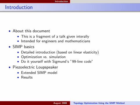
• About this document• This is a fragment of a talk given interally• Intended for engineers and mathematicians
• SIMP basics• Detailed introduction (based on linear elasticity)• Optimization vs. simulation• Do it yourself with Sigmund’s ”99-line code”
• Piezoelectric Loupspeaker• Extended SIMP model• Results
August 2008 Topology Optimization Using the SIMP Method
Introduction
Optimization
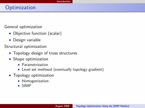
General optimization
• Objective function (scalar)
• Design variable
Structural optimization
• Topology design of truss structures
• Shape optimization• Parametrization• Level set metheod (eventually topology gradient)
• Topology optimization• Homogenization• SIMP
August 2008 Topology Optimization Using the SIMP Method
Classical SIMP Background
Linear elasticity
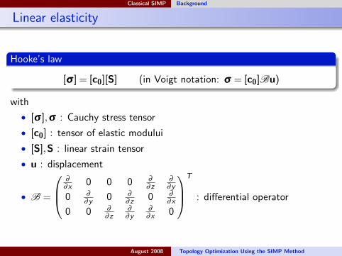
Hooke’s law
[σσσ ] = [c0][S] (in Voigt notation: σσσ = [c0]Bu)
with
• [σσσ ],σσσ : Cauchy stress tensor
• [c0] : tensor of elastic modului
• [S],S : linear strain tensor
• u : displacement
• B =
∂
∂x 0 0 0 ∂
∂z∂
∂y
0 ∂
∂y 0 ∂
∂z 0 ∂
∂x
0 0 ∂
∂z∂
∂y∂
∂x 0
T
: differential operator
August 2008 Topology Optimization Using the SIMP Method
Classical SIMP Background
Strong formulation
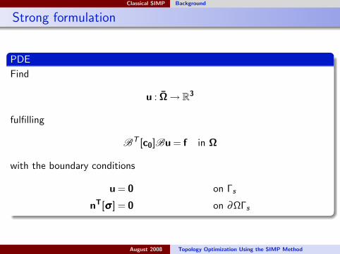
PDE
Find
u : Ω→ R3
fulfilling
BT [c0]Bu = f in Ω
with the boundary conditions
u = 0 on Γs
nT[σσσ ] = 0 on ∂ΩΓs
August 2008 Topology Optimization Using the SIMP Method
Classical SIMP Background
Discrete FEM formulation
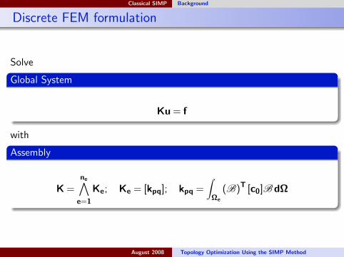
Solve
Global System
Ku = f
with
Assembly
K =ne∧
e=1
Ke; Ke = [kpq]; kpq =∫Ωe
(B)T [c0]BdΩ
August 2008 Topology Optimization Using the SIMP Method
Classical SIMP Incredients
Proportional stiffness model
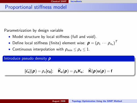
Parametrization by design variable
• Model structure by local stiffness (full and void).
• Define local stiffness (finite) element wise: ρρρ = (ρ1 · · · ρne )T
• Continuous interpolation with ρmin ≤ ρe ≤ 1.
Introduce pseudo density ρρρ
[ce](ρρρ) = ρe [c0]; Ke(ρρρ) = ρeKe; K(ρρρ)u(ρρρ) = f
August 2008 Topology Optimization Using the SIMP Method
Classical SIMP Incredients
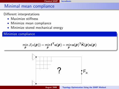
Minimal mean compliance
Different interpretations• Maximize stiffness• Minimize mean compliance• Minimize stored mechanical energy
Minimize compliance
minρρρ
J(u(ρρρ)) = minρρρ
fTu(ρρρ) = minρρρ
u(ρρρ)TK(ρρρ)u(ρρρ)
August 2008 Topology Optimization Using the SIMP Method
Classical SIMP Incredients
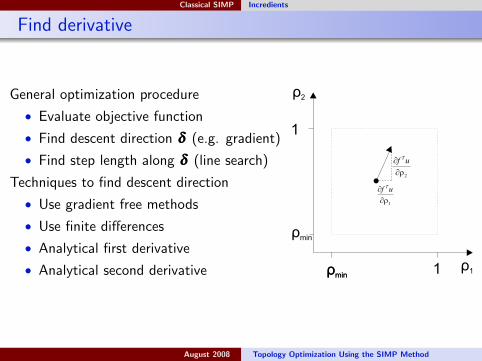
Find derivative
General optimization procedure
• Evaluate objective function
• Find descent direction δδδ (e.g. gradient)
• Find step length along δδδ (line search)
Techniques to find descent direction
• Use gradient free methods
• Use finite differences
• Analytical first derivative
• Analytical second derivative
August 2008 Topology Optimization Using the SIMP Method
Classical SIMP Incredients
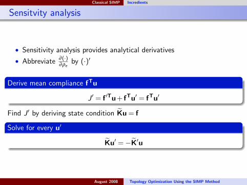
Sensitvity analysis
• Sensitivity analysis provides analytical derivatives
• Abbreviate ∂ (·)∂ρe
by (·)′
Derive mean compliance fTu
J ′ = f ′Tu+ fTu′ = fTu′
Find J ′ by deriving state condition Ku = f
Solve for every u′
Ku′ =−K′u
August 2008 Topology Optimization Using the SIMP Method
Classical SIMP Incredients
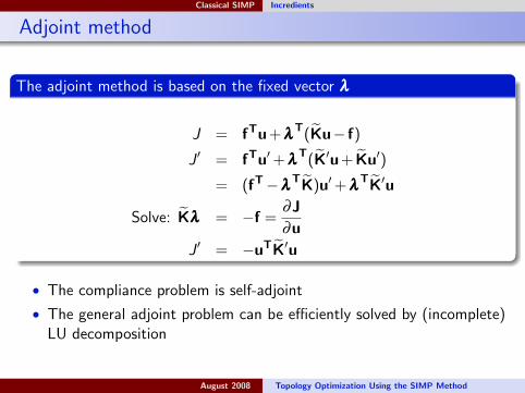
Adjoint method
The adjoint method is based on the fixed vector λλλ
J = fTu+λλλT(Ku− f)
J ′ = fTu′+λλλT(K′u+ Ku′)
= (fT−λλλTK)u′+λλλ
TK′u
Solve: Kλλλ = −f =∂J
∂u
J ′ = −uTK′u
• The compliance problem is self-adjoint
• The general adjoint problem can be efficiently solved by (incomplete)LU decomposition
August 2008 Topology Optimization Using the SIMP Method
Classical SIMP Application of the SIMP method
Naive approach
Minimize compliance: straight forward, initial design 0.5
minρρρ
fTu s.th.: Ku = f ρe ∈ [ρmin : 1] note: Ke = ρeKe, K′e = Ke,
The optimal topology is the trivial solution full material
August 2008 Topology Optimization Using the SIMP Method
Classical SIMP Application of the SIMP method
Naive approach
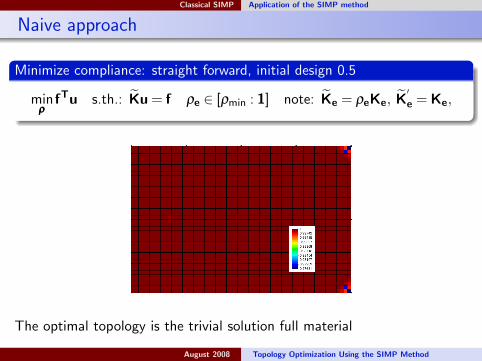
Minimize compliance: straight forward, initial design 0.5
minρρρ
fTu s.th.: Ku = f ρe ∈ [ρmin : 1] note: Ke = ρeKe, K′e = Ke,
The optimal topology is the trivial solution full material
August 2008 Topology Optimization Using the SIMP Method
Classical SIMP Application of the SIMP method
Add constraint
Minimize compliance: volume constraint 50%
minρρρ
fTu s.th.:∫Ω
ρρρ ≤ 1
2V0
“Grey” material has no physical interpretation
August 2008 Topology Optimization Using the SIMP Method
Classical SIMP Application of the SIMP method
Add constraint
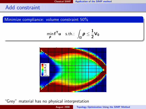
Minimize compliance: volume constraint 50%
minρρρ
fTu s.th.:∫Ω
ρρρ ≤ 1
2V0
“Grey” material has no physical interpretationAugust 2008 Topology Optimization Using the SIMP Method
Classical SIMP Application of the SIMP method
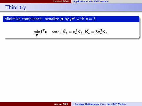
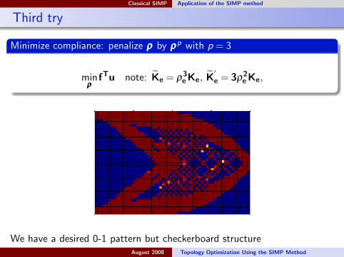
Third try
Minimize compliance: penalize ρρρ by ρρρp with p = 3
minρρρ
fTu note: Ke = ρ3eKe, K
′e = 3ρ
2eKe,
We have a desired 0-1 pattern but checkerboard structure
August 2008 Topology Optimization Using the SIMP Method
Classical SIMP Application of the SIMP method
Third try
Minimize compliance: penalize ρρρ by ρρρp with p = 3
minρρρ
fTu note: Ke = ρ3eKe, K
′e = 3ρ
2eKe,
We have a desired 0-1 pattern but checkerboard structureAugust 2008 Topology Optimization Using the SIMP Method
Classical SIMP Application of the SIMP method
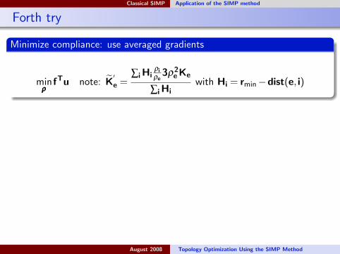
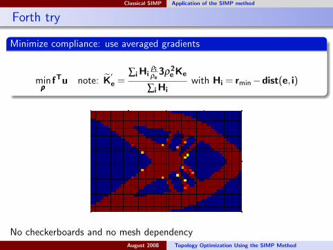
Forth try
Minimize compliance: use averaged gradients
minρρρ
fTu note: K′e =
∑iHiρiρe
3ρ2eKe
∑iHiwith Hi = rmin−dist(e, i)
No checkerboards and no mesh dependency
August 2008 Topology Optimization Using the SIMP Method
Classical SIMP Application of the SIMP method
Forth try
Minimize compliance: use averaged gradients
minρρρ
fTu note: K′e =
∑iHiρiρe
3ρ2eKe
∑iHiwith Hi = rmin−dist(e, i)
No checkerboards and no mesh dependencyAugust 2008 Topology Optimization Using the SIMP Method
Classical SIMP Optimizers
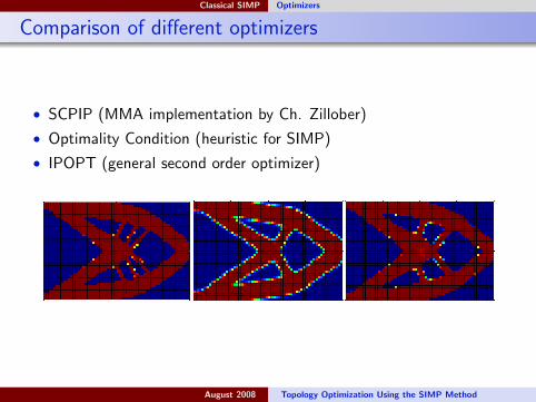
Comparison of different optimizers
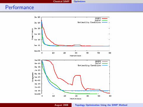
• SCPIP (MMA implementation by Ch. Zillober)
• Optimality Condition (heuristic for SIMP)
• IPOPT (general second order optimizer)
August 2008 Topology Optimization Using the SIMP Method
Classical SIMP Optimizers
Performance
August 2008 Topology Optimization Using the SIMP Method
Classical SIMP Optimizers
Optimality Condition
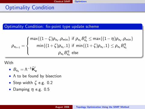
Optimality Condition: fix-point type update scheme
ρek+1=
max(1−ζ )ρek
,ρmin if ρekBη
ek≤max(1−η)ρek
,ρminmin(1+ζ )ρek
,1 if min(1+ζ )ρek,1 ≤ ρek
Bηek
ρekBη
ekelse
With
• Bek= Λ−1K
′e
• Λ to be found by bisection
• Step width ζ e.g. 0.2
• Damping η e.g. 0.5
August 2008 Topology Optimization Using the SIMP Method
Extensions to SIMP Multiple loads
Complex load vs. multiple load cases
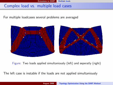
For multiple loadcases several problems are averaged
Figure: Two loads applied simultaniously (left) and seperatly (right)
The left case is instable if the loads are not applied simultaniously
August 2008 Topology Optimization Using the SIMP Method
Extensions to SIMP Multiple loads
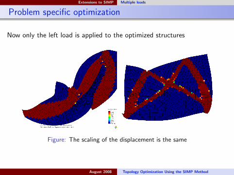
Problem specific optimization
Now only the left load is applied to the optimized structures
Figure: The scaling of the displacement is the same
August 2008 Topology Optimization Using the SIMP Method
Extensions to SIMP Optimization for arbitrary nodes
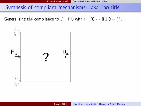
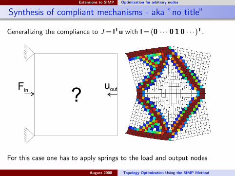
Synthesis of compliant mechanisms - aka ”no title”
Generalizing the compliance to J = lTu with l = (0 · · · 0 1 0 · · ·)T.
For this case one has to apply springs to the load and output nodes
August 2008 Topology Optimization Using the SIMP Method
Extensions to SIMP Optimization for arbitrary nodes
Synthesis of compliant mechanisms - aka ”no title”
Generalizing the compliance to J = lTu with l = (0 · · · 0 1 0 · · ·)T.
For this case one has to apply springs to the load and output nodes
August 2008 Topology Optimization Using the SIMP Method
Extensions to SIMP Harmonic optimization
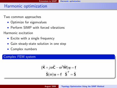
Harmonic optimization
Two common approaches
• Optimize for eigenvalues
• Perform SIMP with forced vibrations
Harmonic excitation
• Excite with a single frequency
• Gain steady-state solution in one step
• Complex numbers
Complex FEM system
(K+ jωC−ω2M)u = f
S(ω)u = f ST
= S
August 2008 Topology Optimization Using the SIMP Method
Extensions to SIMP Harmonic optimization
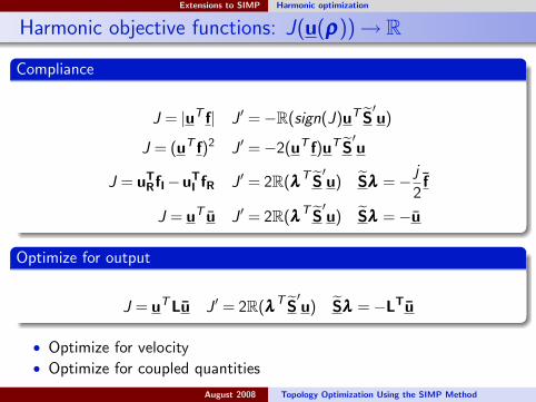
Harmonic objective functions: J(u(ρρρ))→ R
Compliance
J = |uT f| J ′ =−R(sign(J)uT S′u)
J = (uT f)2 J ′ =−2(uT f)uT S′u
J = uTRfI−uT
I fR J ′ = 2R(λλλT S′u) Sλλλ =− j
2f
J = uT u J ′ = 2R(λλλT S′u) Sλλλ =−u
Optimize for output
J = uTLu J ′ = 2R(λλλT S′u) Sλλλ =−LTu
• Optimize for velocity• Optimize for coupled quantities
August 2008 Topology Optimization Using the SIMP Method
Extensions to SIMP Harmonic optimization
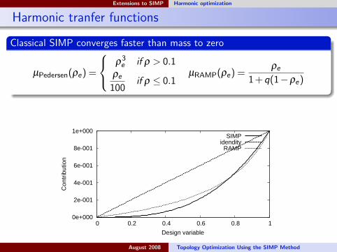
Harmonic tranfer functions
Classical SIMP converges faster than mass to zero
µPedersen(ρe) =
ρ3e if ρ > 0.1
ρe
100if ρ ≤ 0.1
µRAMP(ρe) =ρe
1+q(1−ρe)
0e+000
2e-001
4e-001
6e-001
8e-001
1e+000
0 0.2 0.4 0.6 0.8 1
Con
trib
utio
n
Design variable
SIMPidendity
RAMP
August 2008 Topology Optimization Using the SIMP Method
Extensions to SIMP Harmonic optimization
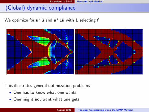
(Global) dynamic compliance
We optimize for uT u and uTLu with L selecting f
This illustrates general optimization problems
• One has to know what one wants
• One might not want what one gets
August 2008 Topology Optimization Using the SIMP Method
Piezoelectricity Model
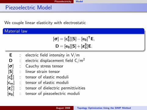
Piezoelectric Model
We couple linear elasticity with electrostatic
Material law
[σσσ ] = [cE0 ][S]− [e0]
TE,
D = [e0][S]+ [εεεS0 ]E.
E : electric field intensity in V/mD : electric displacement field C/m2
[σσσ ] : Cauchy stress tensor[S] : linear strain tensor[cE
0 ] : tensor of elastic moduli[cm] : tensor of elastic moduli[εεεS
0 ] : tensor of dielectric permittivities[e0] : tensor of piezoelectric moduli
August 2008 Topology Optimization Using the SIMP Method
Piezoelectricity Model
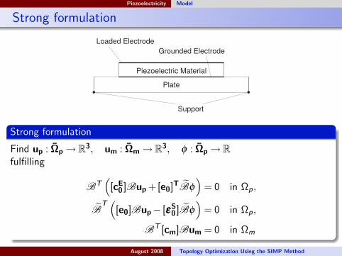
Strong formulation
Grounded Electrode
Loaded Electrode
Plate
Piezoelectric Material
Support
Strong formulation
Find up : Ωp → R3, um : Ωm → R3, φ : Ωp → Rfulfilling
BT([cE
0 ]Bup +[e0]TBφ
)= 0 in Ωp,
BT
([e0]Bup− [εεεS
0 ]Bφ
)= 0 in Ωp,
BT [cm]Bum = 0 in Ωm
August 2008 Topology Optimization Using the SIMP Method
Piezoelectricity Model
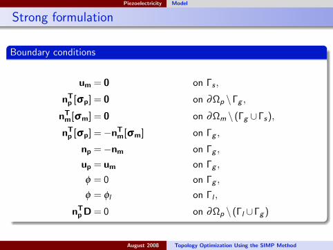
Strong formulation
Boundary conditions
um = 0 on Γs ,
nTp [σσσp] = 0 on ∂Ωp \Γg ,
nTm[σσσm] = 0 on ∂Ωm \ (Γg ∪Γs),
nTp [σσσp] =−nT
m[σσσm] on Γg ,
np =−nm on Γg ,
up = um on Γg ,
φ = 0 on Γg ,
φ = φl on Γl ,
nTp D = 0 on ∂Ωp \ (Γl ∪Γg )
August 2008 Topology Optimization Using the SIMP Method
Piezoelectricity Model
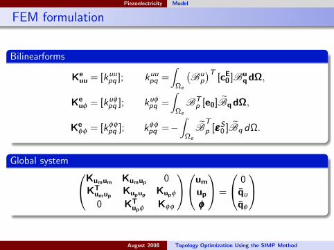
FEM formulation
Bilinearforms
Keuu = [kuu
pq ]; kuupq =
∫Ωe
(Bu
p
)T[cE
0 ]BuqdΩ,
Keuφ = [kuφ
pq ]; kuφpq =
∫Ωe
BTp [e0]BqdΩ,
Keφφ = [kφφ
pq ]; kφφpq =−
∫Ωe
BT
p [εεεS0 ]Bq dΩ.
Global system Kumum Kumup 0KT
umupKupup Kupφ
0 KTupφ
Kφφ
um
up
φφφ
=
0qu
qφ
August 2008 Topology Optimization Using the SIMP Method
SIMP optimization of piezoelectric devices Model
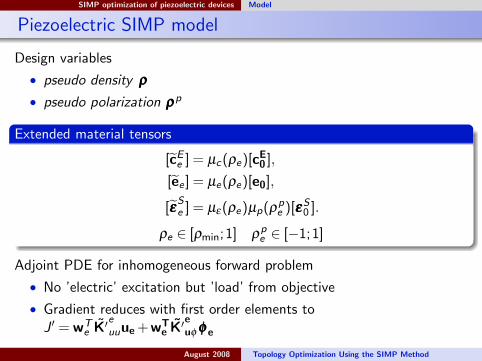
Piezoelectric SIMP model
Design variables
• pseudo density ρρρ
• pseudo polarization ρρρp
Extended material tensors
[cEe ] = µc(ρe)[c
E0 ],
[ee ] = µe(ρe)[e0],
[εεεSe ] = µε(ρe)µp(ρ
pe )[εεεS
0 ].
ρe ∈ [ρmin;1] ρpe ∈ [−1;1]
Adjoint PDE for inhomogeneous forward problem
• No ’electric’ excitation but ’load’ from objective
• Gradient reduces with first order elements toJ ′ = wT
e K′euuue +wT
e K′euφ φφφe
August 2008 Topology Optimization Using the SIMP Method
SIMP optimization of piezoelectric devices Transduction
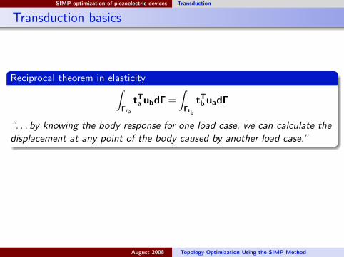
Transduction basics
Reciprocal theorem in elasticity∫Γta
tTa ubdΓ =∫Γtb
tTb uadΓ
“. . . by knowing the body response for one load case, we can calculate thedisplacement at any point of the body caused by another load case.”
Extension to piezoelectricity promisses (Kogl and Silva, 2005):
“. . . the conversion of electrical into elastic energy and vice versa.”
August 2008 Topology Optimization Using the SIMP Method
SIMP optimization of piezoelectric devices Transduction
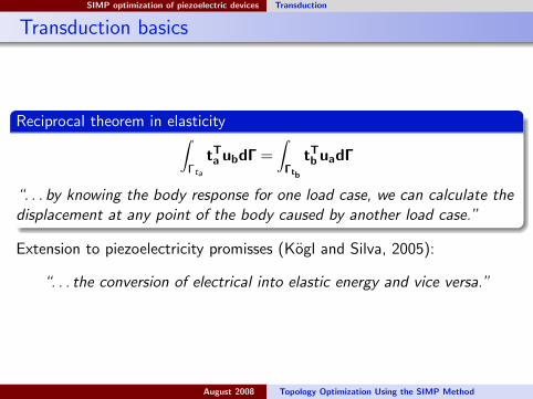
Transduction basics
Reciprocal theorem in elasticity∫Γta
tTa ubdΓ =∫Γtb
tTb uadΓ
“. . . by knowing the body response for one load case, we can calculate thedisplacement at any point of the body caused by another load case.”
Extension to piezoelectricity promisses (Kogl and Silva, 2005):
“. . . the conversion of electrical into elastic energy and vice versa.”
August 2008 Topology Optimization Using the SIMP Method
SIMP optimization of piezoelectric devices Transduction
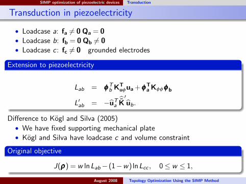
Transduction in piezoelectricity
• Loadcase a: fa 6= 0 Qa = 0• Loadcase b: fb = 0 Qb 6= 0• Loadcase c : fc 6= 0 grounded electrodes
Extension to piezoelectricity
Lab = φφφTb KT
uφua +φφφTa Kφφ φφφb
L′ab = −uTa
K′ub.
Difference to Kogl and Silva (2005)
• We have fixed supporting mechanical plate• Kogl and Silva have loadcase c and volume constraint
Original objective
J(ρρρ) = w lnLab− (1−w) lnLcc , 0≤ w ≤ 1,
August 2008 Topology Optimization Using the SIMP Method
SIMP optimization of piezoelectric devices Transduction
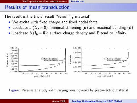
Results of mean transduction
The result is the trivial result “vanishing material”
• We excite with fixed charge and fixed nodal force
• Loadcase a (Qa = 0): minimal stiffening (u) and maximal bending (φ)
• Loadcase b (fb = 0): surface charge density and E tend to infinity
5.0e-006
1.0e-005
1.5e-005
2.0e-005
2.5e-005
3.0e-005
3.5e-005
4.0e-005
4.5e-005
5.0e-005
10 20 30 40 50 60 70 80 90 100
Dis
plac
emen
t (m
)
Area void/piezo (%)
mechanical excitationelectric excitation
1.0e-001
1.0e+000
1.0e+001
1.0e+002
1.0e+003
1.0e+004
10 20 30 40 50 60 70 80 90 100
Vol
tage
(V
)
Area void/piezo (%)
mechanical excitationelectric excitation
Figure: Parameter study with varying area covered by piezoelectric material
August 2008 Topology Optimization Using the SIMP Method
SIMP optimization of piezoelectric devices Results
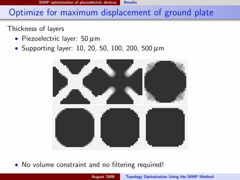
Optimize for maximum displacement of ground plate
Thickness of layers
• Piezoelectric layer: 50 µm
• Supporting layer: 10, 20, 50, 100, 200, 500 µm
• No volume constraint and no filtering required!
August 2008 Topology Optimization Using the SIMP Method
SIMP optimization of piezoelectric devices Results
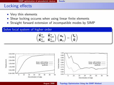
Locking effects
• Very thin elements• Shear locking occures when using linear finite elements• Straight forward extension of incompatible modes by SIMP
Solve local system of higher order(Ke
uu Keuα
Keαu Ke
αα
)(ue
αααe
)=
(fe0
)
0.0e+000
5.0e-005
1.0e-004
1.5e-004
2.0e-004
2.5e-004
3.0e-004
5 10 15 20 25 30 35 40
Dis
plac
emen
t
Discretization of edge
linear, with lockinglinear, locking free
quadratic
0.55
0.60
0.65
0.70
0.75
0.80
0.85
0.90
0.95
1.00
5 10 15 20 25 30 35 40
Vol
ume
frac
tion
Discretization of edge
linear, with lockinglinear, locking free
quadratic
August 2008 Topology Optimization Using the SIMP Method
End
The End
Last comments
• The optimal solution lays inside the PDE (plus adjoint RHS)
• Optimization helps to understand systems better
• Optimization is the next step after simulation
• Thanks for your time!
August 2008 Topology Optimization Using the SIMP Method


![Topology optimization in OpenMDAOm2do.ucsd.edu/static/papers/Hayoung Chung, John T... · Penalization (SIMP) [7]. The other category is the boundary-based formulation ... (2001) [24]](https://img.pdfslide.us/doc/110x75/5ecbc4becdaccc4d425b829e/topology-optimization-in-chung-john-t-penalization-simp-7-the-other-category.jpg)